distribution line model for single-phase-to- ground …
TRANSCRIPT

U.P.B. Sci. Bull., Series C, Vol. 80, Iss. 4, 2018 ISSN 2286-3540
DISTRIBUTION LINE MODEL FOR SINGLE-PHASE-TO-
GROUND FAULT ANALYSIS IN DISTRIBUTION POWER
SYSTEMS
Jinrui TANG1, Jiaqi WANG2, Chen YANG3, Bowen LIU4
Zero-mode transient fault currents are widely used for faulty feeder
identification under single-phase-to-ground fault in neutral non-effectively
grounded distribution systems (NGDSs). Traditional distribution line model is
usually constructed by single π line model, single capacitance or single T
distribution line model. To evaluate the transient simulation effectiveness of the
distribution models, magnitude-frequency and phase-frequency characteristics are
analyzed for the common distribution line models, and sequence parameters of
corresponding distribution line model are analyzed under Karrenbauer
transformation matrix. The analysis and simulation results show that low pass filter
should be installed to filter out the part of signal outside the first capacitive
frequency band, which is calculated by the actual distributed parameter model, and
parameter calculation method for traditional chain-shaped loop circuit of three-
phase line model can also be used for the model presented in this paper.
Keywords: distribution network; single phase-to-ground fault; distribution line
model; faulty feeder identification; zero-mode transient current
1. Introduction
In neutral non-effectively grounded distribution systems (NGDSs), digital
and physical simulation techniques are usually used to obtain zero-mode transient
fault currents in different feeders when single-phase-to-ground fault occurs [1-3].
And then the magnitude and phase characteristics of the transient simulation
signals are analyzed by wavelet transformation or Hilbert transformation to
present new method for single-phase-to-ground faulty feeder identification [4-6].
In the constructed NGDSs simulation models, distribution line models are
mainly divided into two categories: 1) treat the distribution line as a single-to-
ground capacitance [7-10], which is mainly used to simulate the zero-mode
equivalent network. It is simple to realize the simulation and physical distribution
line model using this method and can meet the demand of verifying faulty feeder
identification methods based on steady-state reactive currents and voltages. But its
1 Wuhan University of Technology, China, E-mail: [email protected] 2 Wuhan University of Technology, China, E-mail: [email protected] 3 Wuhan Electric Power Technical College, China 4 Wuhan University of Technology, China

150 Jinrui Tang, Jiaqi Wang, Chen Yang, Bowen Liu
simulation accuracy is not high because the series impedance of the distribution
line has been ignored in this method. 2) apply traditional π-type equivalent
transmission line model into distribution line modeling work. Usually single π line
model is used to represent the distribution line due to its short length [11-14]. This
method has high simulation accuracy in steady-state analysis because the self-
impedance of the distribution line and its positive-sequence, negative-sequence
and zero-sequence network are completely considered in the modeling. But faulty
feeder identification based on transient components are the main measures in the
single-phase-to-ground fault [4-6,9,13-15], and then the applicability of single π
line model used for simulation within thousands of hertz should be discussed
carefully.
In fact, magnitude and phase of the actual distribution line with
distribution parameter vary with frequency. For the single capacitance, single π
and single T line models mentioned above, to ensure that the simulation results
can be used to verify the effectiveness of the presented faulty feeder identification
methods, steady-state and transient response characteristics of the distribution line
models should be analyzed, and their restricted ranges should be defined.
Therefore, the magnitude-frequency and phase-frequency characteristics
of each distribution line model are analyzed, as well as the error in the first
capacitive frequency band, which is calculated by the distributed parameter line
model. Based on this, the parameter calculation method of chain-shaped loop
circuit of three-phase distribution line model is discussed. The research results can
be used to construct a proper distribution line model to study and verify the
single-phase-to-ground fault detection and faulty feeder identification based on
steady-state and transient signals.
2. Magnitude-frequency and phase-frequency characteristics of
distribution line model
2.1 Equivalent input impedance of distribution line model
Once a single-phase-to-ground fault occurs, the fault current and zero-
sequence currents of each feeder are mainly determined by the zero-sequence
network in NGDSs. And the steady-state and transient response characteristics of
the zero-sequence network are mainly influenced by the distribution line.
In the zero-sequence network corresponding to a single-phase-to-ground
fault in NGDSs, the end of the distribution line is at the condition of open circuit.
Assuming the terminal open-circuit voltage equals 2U , the voltage ocU and
current ocI at the front node x from the terminal node can be derived by
2 cosh( )ocU U x= (1)

Distribution line model for single-phase-to-ground fault analysis in distribution power systems 151
2 sinh( )occ
UI x
Z= (2)
where 0 0
0c
R j LZ
j C
+= , which represents the characteristic impedance of the
distribution line, R0, L0 and C0 represent the series resistance, series inductance
and shunt capacitance of the distribution line per unit, and ω equals the angular
frequency.
So, the equivalent input impedance of the distribution line with distributed
parameters at the initial node is
cosh( )
sinh( )
ococ c
oc
U xZ Z
I x
= = (3)
where 0 0( )R j L j C = + , which represents the propagation coefficient of the
distribution line.
For the single capacitance model, the equivalent input impedance at the
initial node is
(1)
0
1( )ocZ j
C x= −
(4)
For the single π model, the equivalent input impedance at the initial node
with an open-circuit terminal node is
0 00 0(2)
0 00
2 2( )
( )4oc
R x j L x j jC x C x
Z
R x j L x jC x
+ − −
=
+ −
(5)
For the single T model, the equivalent input impedance at the initial node
with an open-circuit terminal node is
(3)0 0
0
1( )
2 2oc
x xZ R j L j
C x= + −
(6)
The equivalent input impedances of different distribution line models with
open-circuit terminal node, which include single capacitance, single π and single
T models, are given in equations (3), (4), (5) and (6) separately.
2.2 Magnitude-frequency and phase-frequency characteristics of each
distribution line model
In this paper, typical parameters of distribution overhead lines and cables
shown in Table 1 is used to analyze the magnitude-frequency and phase-
frequency characteristics of each distribution line model [16]. The difference in
the equivalent input impedance is calculated for x=2 km, 5km, 10 km, and 20 km,
and some results are shown in Figs. 1-4.

152 Jinrui Tang, Jiaqi Wang, Chen Yang, Bowen Liu
To evaluate the difference in the phase of equivalent input impedance
among single capacitance model, single π model, single T model, and distributed
parameter model under the steady-state and transient response, the upper limit
value fm of the first capacitive frequency band is used to represent the diversity,
which means the frequency corresponding to the initial conversion of the phase
varies from -90° to 90°.
To evaluate the difference in the magnitude of equivalent input impedance
for each distribution line model under the steady-state and transient response, the
magnitude difference coefficient Ez is used to state the diversity, which should be
calculated by the following equation (7)
2
1
, ,( )
f
z i f s ff f
E E E f
=
= − (7)
where Ei,f denotes the magnitude of the input impedance corresponding to model i
at frequency f, and Es,f denotes the magnitude of input impedance corresponding
to the distributed parameter line model at frequency f; Δf denotes the frequency
calculation step used in the analysis; f1 and f2 are used to represent the lower and
upper frequency limits of the analyzed frequency band respectively.
According to the typical single-phase-to-ground faulty feeder
identification methods based on transient signals presented in literatures [4-
6,9,13-15, 17-18], f1 could be set as 50 Hz, and f2 could be set as min. (5000 Hz,
fm).
From Figs. 1-4, it could be derived that there is large difference in the
phase of the input impedance between single capacitance model and distributed
parameter model. The phase corresponding to the single capacitance model
always equals -90°, and the phase corresponding to the distributed parameter
model varies periodically from +90° to -90° or on the contrary.
Table 1
Typical sequence parameters of distribution overhead lines and cables
Positive Negative Zero
R
[Ω/km]
L
[mH/km]
C
[μF/km]
R
[Ω/km]
L
[mH/km]
C
[μF/km]
R
[Ω/km]
L
[mH/km]
C
[μF/km]
Distribution
overhead line 0.096 1.22 0.011 0.096 1.22 0.011 0.23 3.66 0.007
Distribution
cable 0.11 0.52 0.29 0.11 0.52 0.29 0.34 1.54 0.19

Distribution line model for single-phase-to-ground fault analysis in distribution power systems 153
(a) magnitude-frequency characteristic; (b) phase-frequency characteristic
Fig. 1. Curves between parameter and frequency for distribution overhead line with length of 5km
(a) magnitude-frequency characteristic; (b) phase-frequency characteristic
Fig. 2. Curves between parameter and frequency for distribution cable with length of 5km
(a) magnitude-frequency characteristic; (b) phase-frequency characteristic
Fig.3. Curves between parameter and frequency for distribution overhead line with length of 20km
154 Jinrui Tang, Jiaqi Wang, Chen Yang, Bowen Liu
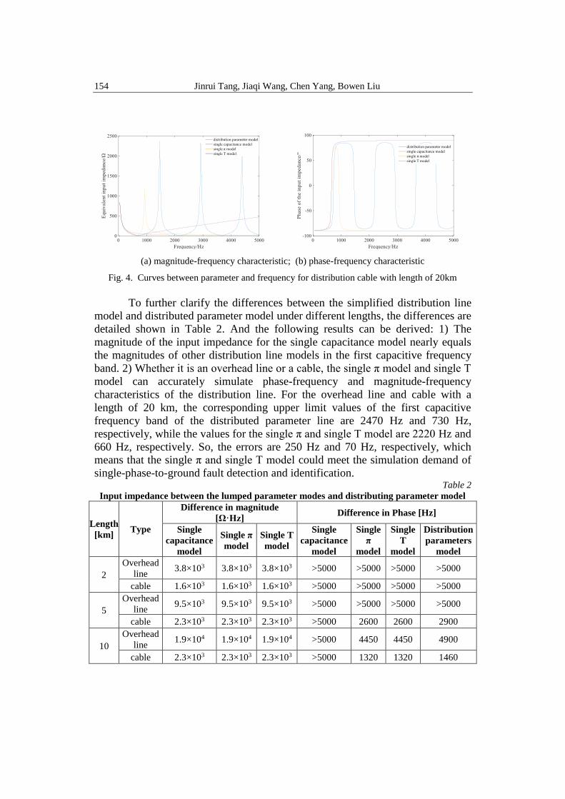
(a) magnitude-frequency characteristic; (b) phase-frequency characteristic
Fig. 4. Curves between parameter and frequency for distribution cable with length of 20km
To further clarify the differences between the simplified distribution line
model and distributed parameter model under different lengths, the differences are
detailed shown in Table 2. And the following results can be derived: 1) The
magnitude of the input impedance for the single capacitance model nearly equals
the magnitudes of other distribution line models in the first capacitive frequency
band. 2) Whether it is an overhead line or a cable, the single π model and single T
model can accurately simulate phase-frequency and magnitude-frequency
characteristics of the distribution line. For the overhead line and cable with a
length of 20 km, the corresponding upper limit values of the first capacitive
frequency band of the distributed parameter line are 2470 Hz and 730 Hz,
respectively, while the values for the single π and single T model are 2220 Hz and
660 Hz, respectively. So, the errors are 250 Hz and 70 Hz, respectively, which
means that the single π and single T model could meet the simulation demand of
single-phase-to-ground fault detection and identification. Table 2
Input impedance between the lumped parameter modes and distributing parameter model
Length
[km] Type
Difference in magnitude
[Ω·Hz] Difference in Phase [Hz]
Single
capacitance
model
Single π
model
Single T
model
Single
capacitance
model
Single
π
model
Single
T
model
Distribution
parameters
model
2
Overhead
line 3.8×10³ 3.8×10³ 3.8×10³ >5000 >5000 >5000 >5000
cable 1.6×10³ 1.6×10³ 1.6×10³ >5000 >5000 >5000 >5000
5
Overhead
line 9.5×10³ 9.5×10³ 9.5×10³ >5000 >5000 >5000 >5000
cable 2.3×10³ 2.3×10³ 2.3×10³ >5000 2600 2600 2900
10
Overhead
line 1.9×10⁴ 1.9×10⁴ 1.9×10⁴ >5000 4450 4450 4900
cable 2.3×10³ 2.3×10³ 2.3×10³ >5000 1320 1320 1460

Distribution line model for single-phase-to-ground fault analysis in distribution power systems 155
20
Overhead
line 1.9×10⁴ 1.9×10⁴ 1.9×10⁴ >5000 2220 2220 2470
cable 2.0×10³ 2.0×10³ 2.0×10³ >5000 660 660 730
Annotation: magnitude difference refers to the sum of the difference in magnitude within the
interval from the industrial frequency to the upper limit of the capacitive frequency band, and the
phase difference refers to the comparison of the upper limit frequency of the first capacitive
frequency band.
Therefore, a low-pass filter should be added to filter out the signal outside
the first capacitive frequency band when single capacitance, single π or single T
distribution model is used to construct the distribution power system. The
parameters of the low-pass filter can be identified with reference to the upper limit
value of the first capacitive frequency band.
3. Parameter calculation method for three-phase distribution line model
3.1 Chain-shaped loop circuit model of three-phase distribution line
Since the medium-voltage power distribution line consists of three-phase
AC lines, each phase has its self-impedance, and mutual inductance and
capacitance also exist between the phase and phase, as well as between the phase
and the earth. When lumped parameters are used to simulate the distributed
parameter line, the mutual connection should be considered. At present, chain-
shaped loop circuit model is usually used to construct the three-phase AC lines,
which is shown in Fig. 5.
In Fig. 5, L1, R1, C1, and l represent the positive-sequence self-inductance,
positive-sequence resistance, positive-sequence capacitance, and distribution line
length, respectively; CN, LN and RN should be obtained by equations (8) and (9) [19]. That is, CN, LN and RN are identified by the positive-sequence parameters and
zero-sequence parameters of the distribution line to ensure that chain-shaped loop
circuit model can accurately simulate the zero-sequence parameter of the actual
distribution line.
L1l R1l
LNl RNl0.5CNl 0.5CNl
0.5C1l 0.5C1l
Fig. 5. Chain-shaped loop circuit of three-phase distribution line model

156 Jinrui Tang, Jiaqi Wang, Chen Yang, Bowen Liu
1 0
1 0
3N
C CC
C C=
− (8)
0 1 0 1,3 3
N NL L R R
L R− −
= = (9)
where L0, R0, and C0 are the zero-sequence self-inductance, zero-sequence
resistance, and zero-sequence capacitance of the distribution line, respectively.
3.2 Parameter calculation for Chain-shaped loop circuit model of Distribution
Line
It is important to note that the positive-sequence and zero-sequence
impedances given in equations (8) and (9) are calculated from the principle of the
traditional symmetric component method. But in the transient analysis, response
should be analyzed under a wide frequency range from power frequency to
several kilohertz. And then Karrenbauer transformation should be used to identify
the parameters [20].
Taking a three-phase lossless line as an example, the voltage and current
can be expressed as a function of time t and distance x, which are shown as
follows
A A
s m mB B
m s m
m m sC C
u i
x tL L Lu i
L L Lx t
L L Lu i
x t
− =
(10)
A A
s m mB B
m s m
m m sC C
i u
x xk k ki u
k k kx x
k k ki u
x x
− =
(11)
where ks equals C0+2Cm; km equals -Cm; Ls represents the series inductance of
each phase conductor; Lm is the mutual inductance between one phase to another
phase conductor; C0 is the phase-to-ground capacitance, Cm is the phase-to-phase
capacitance; x is the distance from the node to the terminal, uA、uB、uC are
instantaneous voltages of phase A, B and C, respectively; iA、iB, and iC are
instantaneous currents of phase A, B and C, respectively.
Equations (10) and (11) can be rewritten in matrix form as

Distribution line model for single-phase-to-ground fault analysis in distribution power systems 157
x t
− =
u iL (12)
x t
− =
i uC (13)
Since there are nonzero off-diagonal elements in L and C matrix in
equations (12) and (13), it is not easy to solve the equations. And then coordinate
transformation should be applied to change off-diagonal elements of the
coefficient matrix to zero. Both symmetric component transformation and
Karrenbauer transformation can be used as the proper transformation.
For traditional symmetric component transformation, assuming
2
2
1 1 1
1
1m m
a a
a a
= = =
u iS
u i (14)
where S represents the transformation matrix; u=[uA,uB,uC]T; i=[iA,iB,iC]T;
um=[u0,u+,u-]T; im=[i0,i+,i-]
T. Among them, symbol 0, symbol + and symbol -
represent zero sequence, positive sequence and negative sequence, respectively.
And the variable a equals e-120° in the matrix.
Then equation (15) can be derived
2 2 21
2 2 2
2 2 21
2 2 2
m m mu
m m mi
x t t
x t t
−
−
= =
= =
u u uS LCS D
i i iS LCS D
(15)
where
( 2 )( 2 ) 0 0
0 ( )( ) 0
0 0 ( )( )
u i
s m s m
s m s m
s m s m
L L K K
K K L L
K K L L
= = =
+ +
= − − − −
-1D D S LCS
(16)
Therefore, for sequence parameters in the symmetric component
transformation, the following results can be obtained: L0=Ls+2Lm, C0=Ks+2Km,
L1=L2=Ls-Lm, C1= C2=Ks-Km.
For Karrenbauer transformation, assuming
(2)
1 1 1
1 2 1
1 1 2m m
= = = − −
u iS
u i (17)
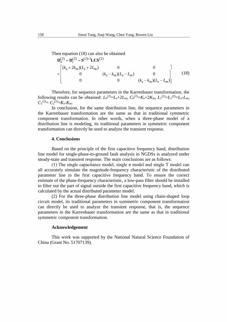
158 Jinrui Tang, Jiaqi Wang, Chen Yang, Bowen Liu
Then equation (18) can also be obtained (2)(2) (2)-1 (2)
( 2 )( 2 ) 0 0
0 ( )( ) 0
0 0 ( )( )
u i
s m s m
s m s m
s m s m
k k L L
k k L L
k k L L
= =
+ +
= − − − −
D D S LCS
(18)
Therefore, for sequence parameters in the Karrenbauer transformation, the
following results can be obtained: L0(2)=Ls+2Lm, C0
(2)=Ks+2Km, L1(2)=L2
(2)=Ls-Lm,
C1(2)= C2
(2)=Ks-Km.
In conclusion, for the same distribution line, the sequence parameters in
the Karrenbauer transformation are the same as that in traditional symmetric
component transformation. In other words, when a three-phase model of a
distribution line is modeling, its traditional parameters in symmetric component
transformation can directly be used to analyze the transient response.
4. Conclusions
Based on the principle of the first capacitive frequency band, distribution
line model for single-phase-to-ground fault analysis in NGDSs is analyzed under
steady-state and transient response. The main conclusions are as follows:
(1) The single capacitance model, single π model and single T model can
all accurately simulate the magnitude-frequency characteristic of the distributed
parameter line in the first capacitive frequency band. To ensure the correct
estimate of the phase-frequency characteristic, a low-pass filter should be installed
to filter out the part of signal outside the first capacitive frequency band, which is
calculated by the actual distributed parameter model.
(2) For the three-phase distribution line model using chain-shaped loop
circuit model, its traditional parameters in symmetric component transformation
can directly be used to analyze the transient response, that is, the sequence
parameters in the Karrenbauer transformation are the same as that in traditional
symmetric component transformation.
Acknowledgement
This work was supported by the National Natural Science Foundation of
China (Grant No. 51707139).

Distribution line model for single-phase-to-ground fault analysis in distribution power systems 159
R E F E R E N C E S
[1]. Yankan Song, Ying Chen, Shaowei Huang, et al. Fully GPU-based electromagnetic transient
simulation considering large-scale control systems for system-level studies[J]. IET
Generation, Transmission& Distribution, 2017, 11(11): 2840-2851.
[2]. Jorge Jardim, Karen Caino de Oliveira Salim, Pedro Henrique Lourenco dos Santos, et al.
Variable time step application on hybrid electromechanical-electromagnetic simulation[J].
IET Generation, Transmission & Distribution, 2017, 11(12): 2968-2973.
[3]. Nagy I. Elkalashy, Matti Lehtonen, Hatem A. Darwish, et al. Modeling and experimental
verification of high impedance arcing fault in medium voltage networks[J]. IEEE
Transactions on Dielectrics and Electrical Insulation, 2007, 14(2): 375-383.
[4]. Yongduan Xue, Xiaoru Chen, Huamao Song, et al. Resonance analysis and faulty feeder
identification of high-impedance faults in a resonant grounding system[J]. IEEE
Transactions on Power Delivery, 2017, 32(3): 1545-1555.
[5]. Yuanyuan Wang, Yuhao Huang, Xiangjun Zeng, et al. Faulty feeder detection of single phase-
earth fault using grey relation degree in resonant grounding system[J]. IEEE Transactions
on Power Delivery, 2017, 32(1): 55-61.
[6]. Jinrui Tang, Xianggen Yin, Minghao Wen, et al. Fault location in neutral non-effectively
grounded distribution systems using phase current and line-to-line voltage[J]. Electric
Power Components and Systems, 2014, 42(13): 1371-1385.
[7]. Peng Wang, Baichao Chen, Cuihua Tian, et al. A novel neutral electromagnetic hybrid
flexible grounding method in distribution networks[J]. IEEE Transactions on Power
Delivery, 2017, 32(3): 1350-1358.
[8]. Wen Wang, Lingjie Yan, Xiangjun Zeng, et al. Principle and design of a single-phase inverter-
based grounding system for neutral-to-ground voltage compensation in distribution
networks[J]. IEEE Transactions on Industrial Electronics, 2017, 64(2): 1204-1213.
[9]. M.F. Abdel-Fattah, M. Lehtonen. Transient algorithm based on earth capacitance estimation
for earth-fault detection in medium-voltage networks[J]. IET Generation, Transmission &
Distribution, 2012, 6(2): 161-166.
[10].N. Kolcio, J.A. Halladay, G.D. Allen, et al. Transient overvoltages and overcurrents on
12.47kV distribution lines: computer modeling results[J]. IEEE Transactions on Power
Delivery, 1993, 8(1): 359-366.
[11].Ye Cheng, Zhigang Liu, Ke Huang. Transient analysis of electric arc burning at insulated rail
joints in high-speed railway stations based on state-space modeling[J]. IEEE Transactions
on Transportation Electrification, 2017, 3(3): 750-761.
[12].Peng Wang, Baichao Chen, Hong Zhou, et al. Fault location in resonant grounded network by
adaptive control of neutral-to-earth complex impedance[J]. IEEE Transactions on Power
Delivery, 2018, 33(2): 689-698.
[13].Amir Farughian, Lauri Kumpulainen, Kimmo Kauhaniemi. Review of methodologies for
earth fault indication and location in compensated and unearthed MV distribution
networks[J]. Electric Power Systems Research, 2018(154): 373-380.
[14].A. Bahmanyar, S. Jamali, A. Estebsari, et al. A comparison framework for distribution system
outage and fault location methods[J]. Electric Power Systems Research, 2017(145): 19-34.
[15].Tao Cui, Xinzhou Dong, Zhiqian Bo, et al. Hilbert-transform-based transient/intermittent
earth fault detection in noneffectively grounded distribution systems, 2011, 26(1): 143-151.
[16].Jinrui Tang, Chen Yang, Lijun Cheng. Analysis on zero-sequence current variation
characteristic for feeders of distribution network at different residual current compensation
factors[J]. Automation of Electric Power Systems, 2017, 41(13): 125-132. (in Chinese)

160 Jinrui Tang, Jiaqi Wang, Chen Yang, Bowen Liu
[17].Hongchun Shu, Shixin Peng, Bin Li, et al. A new approach to detect fault line in resonant
earthed system using simulation after test[J]. Proceedings of the CSEE, 2008, 28(16): 59-
64. (in Chinese)
[18].Jianwen Zhao, Yongjia Liu, Jing Liang, et al. Fault line selection based on improved FastICA
and Romanovsky guidelines[J]. Proceedings of the CSEE, 2016, 36(19): 5209-5218.
[19].Panos C. Kotsampopoulos, Vasilis A. Kleftakis, Nikos D. Hatziargyriou. Laboratory education
of modern power systems using PHIL simulation[J]. IEEE Transactions on Power Systems,
2017, 32(5): 3992-4001.
[20].Shicong Ma, Bingyin Xu, Houlei Gao, et al. An improved differential equation method for
earth fault location in non-effectively earthed system[C]. 10th IET International Conference
on Developments in Power System Protection, Manchester, UK, 2010.