ORE Open Research Exeter

TITLE

Distribution and mass of diffuse and dense CO gas in the Milky Way

AUTHORS

Roman-Duval, J; Heyer, M; Brunt, C; et al.

JOURNAL

The Astrophysical Journal

DEPOSITED IN ORE

17 February 2016

This version available at

https://ore.exeter.ac.uk/repository

COPYRIGHT AND REUSE

Open Research Exeter makes this work available in accordance with publisher policies.

A NOTE ON VERSIONS

The version presented here may differ from the published version. If citing, you are advised to consult the published version for pagination, volume/issue and date ofpublication

DISTRIBUTION AND MASS OF DIFFUSE AND DENSE CO GAS IN THE MILKY WAY

Julia Roman-Duval1, Mark Heyer2, Christopher M. Brunt3, Paul Clark4, Ralf Klessen5, and Rahul Shetty51 Space Telescope Science Institute, 3700 San Martin Drive, Baltimore, MD 21218, USA; duval@stsci.edu

2 Department of Astronomy, Lederle Research Building, University of Massachusetts, Amherst, MA 01003, USA3 Astrophysics Group, School of Physics, University of Exeter, Stocker Road, Exeter EX4 4QL, UK

4 School of Physics and Astronomy, Queens Buildings, The Parade, Cardiff University, Cardiff, CF24 3AA, UK5 Universität Heidelberg, Zentrum für Astronomie, Institut für Theoretische Astrophysik, Albert-Ueberle-Strasse 2, D-69120 Heidelberg, Germany

Received 2015 October 2; accepted 2016 January 4; published 2016 February 17

ABSTRACT

Emission from carbon monoxide (CO) is ubiquitously used as a tracer of dense star-forming molecular clouds.There is, however, growing evidence that a significant fraction of CO emission originates from diffuse moleculargas. Quantifying the contribution of diffuse CO-emitting gas is vital for understanding the relation betweenmolecular gas and star formation. We examine the Galactic distribution of two CO-emitting gas components, ahigh column density component detected in 13CO and 12CO, and a low column density component detected in12CO, but not in 13CO. The “diffuse” and “dense” components are identified using a combination of smoothing,masking, and erosion/dilation procedures, making use of three large-scale 12CO and 13CO surveys of the inner andouter Milky Way. The diffuse component, which globally represents 25% (1.5×108Me) of the total moleculargas mass (6.5 108´ Me), is more extended perpendicular to the Galactic plane. The fraction of diffuse gasincreases from ∼10%–20% at a galactocentric radius of 3–4 kpc to 50% at 15 kpc, and increases with decreasingsurface density. In the inner Galaxy, a yet denser component traced by CS emission represents 14% of the totalmolecular gas mass traced by 12CO emission. Only 14% of the molecular gas mass traced by 12CO emission isidentified as part of molecular clouds in 13CO surveys by cloud identification algorithms. This study indicates thatCO emission not only traces star-forming clouds, but also a significant diffuse molecular ISM component.

Key words: ISM: atoms – ISM: clouds – ISM: molecules – ISM: structure

1. INTRODUCTION

Stars are born from the fragmentation and collapse of densecores within molecular clouds. While the formation of starswithin cores is dominated by gravity and is reasonably wellunderstood, the mechanisms by which molecular clouds andmolecular gas form and evolve remain an open question. Forinstance, it is not clear whether molecular clouds are long-livedgravitationally bound entities or transient over-densities in theunderlying turbulent flow. The roles of radiative transfer,chemistry, magnetic fields, and hydrodynamics in shaping thestructure and composition of molecular gas are also poorlyconstrained (Mac Low & Klessen 2004; Klessen & Glo-ver 2014). Understanding the physics of the molecular gas, andthereby the formation of stars, is crucial for comprehendinggalaxy formation and evolution.

Molecular hydrogen (H2) is an inefficient radiator within thecold environments of molecular clouds. Rotational emissionfrom carbon monoxide (CO), the most abundant molecule inthe dense phase after H2, is widely used as a tracer of moleculargas instead. It is usually assumed that CO emission tracesdense, well-shielded molecular gas that is or will be formingstars. However, there is growing evidence that a significantfraction of CO emission originates from relatively diffuse, non-star-forming molecular gas. For example, Goldsmith et al.(2008) determine that 40% of the molecular gas mass in theTaurus molecular cloud resides in diffuse molecular gas(N(H2) < 2.5×1021 cm−2) that is detected in the 12CO line,but not the 13CO line, and is not forming stars. Based onobservations toward select sight-lines in the Milky Way, Lisztet al. (2010) determine a similar (40%) fraction of diffuse non-star-forming 12CO-bright molecular gas. They conclude thatthe CO-to-H2 conversion factor of this diffuse component is no

different from the conversion factor of the dense gas (XCO =2 1020´ cm−2 K−1 km−1 s). In M51, Pety et al. (2013)quantify the distribution and mass of 12CO-bright moleculargas, and conclude that 50% of the CO emission originates fromrelatively low column density (<1022 cm−2) molecular gas onapproximately Kiloparsec scales.Studies of the Kennicutt–Schmidt (K-S) relation

(Schmidt 1959; Kennicutt 1998) between molecular gas andstar formation in Galactic (Heiderman et al. 2010) andextragalactic (Krumholz et al. 2012; Federrath 2013; Shettyet al. 2014b; Salim et al. 2015) environments also infer from thescale-dependence of the K-S relation that a significant fraction ofmolecular gas must be in diffuse non-star-forming phase. If theK-S relation is sub-linear, the fraction of dense star-forming gasmust decrease as the disk surface density increases, leading tolonger molecular gas depletion times in higher surface densitydisks. Conversely, a super-linear K-S relation implies that thedense gas fraction increases and that molecular depletion timesdecrease with increasing surface density. Previous studies of theK-S relation in nearby galaxies have reported a range of K-Sslopes, from super-linear (Liu et al. 2011; Momose et al. 2013),to linear (Bigiel et al. 2008; Leroy et al. 2013), to sub-linear(Blanc et al. 2009; Ford et al. 2013; Shetty et al. 2013, 2014b).Quantifying the contribution and distribution of diffuse CO-emitting molecular gas therefore has important implications forour understanding of the processes leading to star formation andthus to galaxy evolution.While the Milky Way offers the best spatial resolution to

study this issue, quantifying the contribution of diffusemolecular gas is problematic in our own Galaxy. First, it isdifficult to accurately estimate a distance to a parcel ofmolecular gas, due to the kinematic distance ambiguity, thelarge uncertainties on kinematic distances due to non-circular

The Astrophysical Journal, 818:144 (19pp), 2016 February 20 doi:10.3847/0004-637X/818/2/144© 2016. The American Astronomical Society. All rights reserved.

1

motions, and due to confusion in velocity space of near and farmolecular clouds along the line of sight. To circumvent someof these issues, studies of the distribution and properties ofmolecular gas in the Milky Way (e.g., Solomon et al. 1987;Rathborne et al. 2009; Roman-Duval et al. 2010) are forced tobreak up the CO emission in discrete molecular cloudsidentified by various available cloud identification algorithmssuch as CLUMPFIND (Williams et al. 1994), dendrograms(Rosolowsky et al. 2008), or GAUSSCLUMP (Stutzki 2014).The drawback of this approach is of course that such detectionalgorithms would exclude diffuse CO emission. A detailed,high-resolution study of CO emission in the Milky Way is thusneeded to better understand the spatial distribution of dense anddiffuse molecular gas. This is possible with surveys acquiredsince the 2000s.

In this paper, we (re-)examine the luminosity and surfacedensity distribution of CO-emitting gas in the inner (inside thesolar circle) and outer (outside the solar circle) Milky Way,based on the Galactic Ring Survey (GRS) of 13CO emission,the University of Massachusetts Stony Brook (UMSB) 12COsurvey, and the Exeter-FCRAO (EXFC) survey (12CO and13CO). In particular, we derive the spatial distribution (inluminosity and surface density) of three CO-emitting gascomponents in the Milky Way. Our study covers theGalactocentric radius range 3–15 kpc (and so excludes theGalactic Center). We identify gas that is detected in the 12COline but shows no emission in the 13CO line as the “diffuseextended” component. We define the “dense” component as thegas detected in both 12CO and 13CO lines in the same voxel.Last, the “very dense” component corresponds to the gasdetected in 12CO, 13CO, and carbon mono-sulfide (CS) 2-1 lineemission. The CO-emitting gas components observed withthese different tracers correspond to different density regimesbecause their critical densities are different. The critical densityof the 12CO and 13CO 1-0 lines are similar at about2×103 cm−3, while the critical density of the CS 2-1 line is5×105 cm−3. However, due to optical depth effects (radiativetrapping), the effective critical density of the 12CO, 13CO, andCS lines are closer to ∼102 cm−3, 103 cm−3, and a few104 cm−3. Additionally, we ensure that the signal-to-noise ratio(S/N) of the detection threshold is consistent for all three lines,so that the relative contributions of the three CO gascomponents independent of the native sensitivities of thesurveys.

The paper is organized as follows. Section 2 describes theobservations. In the subsequent Section 3, we describe themethod to identify voxels (i.e., ℓ, b, v position) with significantemission, and estimate the distances and other physicalproperties of the emitting regions, such as excitation tempera-tures and column densities. Section 4 presents the derivedproperties, including the radial (with Galactocentric radius) andvertical (above and below the Galactic plane) distributions ofdiffuse, dense, and very dense components. Following adiscussion of some limitations and implications of our analysisin Section 5, we conclude with a summary in Section 6.

2. OBSERVATIONS

2.1. Observations of the 12CO J = 1 0 Line in the InnerGalaxy: University of Massachusetts Stony Brook Survey

In the inner Galaxy, the 12CO line was observed as part ofthe UMSB survey (Clemens et al. 1986; Sanders et al. 1986), a

joint program between FCRAO and the State University ofNew York at Stony Brook performed between 1981 Novemberand 1984 March. All of the observations were obtained usingthe FCRAO 14 m telescope. A grid sampled every 3′ coveringthe range 18°< ℓ < 55°, and −1°< b < +1° was observedwith a velocity resolution of 1 km s−1 and an angular resolutionof 45″. The UMSB survey covers the velocity range−10 km s−1 < VLSR < 140 km s−1. The data were convertedfrom radiation temperature scale (TR*) to a main beamtemperature scale (TMB) via TMB = TR*/0.7.

2.2. Observations of the 13CO J = 1 0 Linein the Inner Galaxy: GRS

The GRS survey observed a ∼40° section of the inner galaxy(18° ℓ 55°.7, −1° b 1°) in 13CO J = 1 0 , usingthe FCRAO. The observations were taken between 1998 and2005 with the SEQUOIA multipixel array. The surveyachieved an angular esolution of 47″, sampled on a 22″ grid,and a spectral resolution of 0.212 km s−1 for a noise varianceper voxel of σ(TA*) = 0.13 K ( 0.24TMBs = K accounting for themain beam efficiency of 0.48). The survey covers the range ofvelocity −5 to 135 km s−1 for Galactic longitudes ℓ 40° and−5 to 85 km s−1 for Galactic longitudes ℓ 40°. The data wereconverted from the antenna temperature scale TA* to a mainbeam temperature scale TMB by correcting for the main beamefficiency of 0.48.

2.3. Observations of the CS 2 1 Linein the Inner Galaxy: GRS

The GRS survey observed the CS 2 1 line in a two-square-degree field located at Galactic longitudesℓ=44°.3–46°.3 and Galactic latitudes b = −0°.5–0°.5, withthe same velocity coverage as the 13CO (−5 to 85 km s−1). Asfor the 13CO survey, the CS survey is also half-beam-sampled(45″ resolution with 22″ pixels). It achieved a sensitivity of

T 0.13A( )*s = K per voxel. The data were converted from theantenna temperature scale TA* to a main beam temperature scaleTMB by correcting for the main beam efficiency of 0.48.

2.4. Observations of the 12CO and 13CO J = 1 0 Linesin the outer Galaxy: Exeter-FCRAO (EXFC) Survey

Data for the EXFC survey (C. M. Brunt et al. 2015, inpreparation) were observed between 2003 and 2006 with theSEQUOIA beam array receiver. The survey spans twolongitude ranges: ℓ=55°–100° (hereafter EXFC 55–100),with the Galactic Latitude range −1°.4 b +1°.9, andℓ=135°–195° (hereafter EXFC 135–195), in the Galacticlatitude range −3°.6 b +5°.6. The EXFC 135–195 surveycovers the outer Galaxy only, while the EXFC 55–100 coversboth the inner and outer Galaxy. 12CO and 13CO 1-0 wereobserved simultaneously with angular resolutions of 45″ and48″, sampled on a 22 5 grid, and a spectral resolution of0.127 km s−1. The data were de-convolved to remove con-tributions by the antenna error beam and so are implicitly on amain beam temperature scale. We do not use the longituderange ℓ=165°–195° because the radial velocity of COemission in this range is close to zero, independent of distance(almost purely tangential motion).

2

The Astrophysical Journal, 818:144 (19pp), 2016 February 20 Roman-Duval et al.

2.5. Mosaicking and Regridding

The EXFC observations were split into 75 fields, samplingGalactic longitudes 55°–100° and 135°–195° every 3°. In thisanalysis, we do not use data with Galactic longitudes 165°,because at those longitudes the motion of the gas is almostpurely transverse (no radial velocity component), and akinematic distance can therefore not be estimated robustly.We resample and mosaic the full EXFC coverage belowℓ=165° into 13 disjoint mosaic fields spanning 5° inlongitude and the full latitude range of EXFC (−3°.6–5°.6 forEXFC 135–195, −1°.4–1°.9 for EXFC 55–100). The individualspectra composing the mosaics are weighted by their rms mainbeam temperature to produce the mosaics, and the originalangular (22 5) and spectral (0.127 km s−1) sampling areconserved. Due to i/o and memory limitations, the entiresurvey cannot be stored into a single mosaic file.

The GRS and UMSB surveys roughly cover the same area(ℓ;18°–55°, b ;−1°–1°). However, small differences existin the mapping strategy between the 12CO and 13CO surveys,the GRS being half-beam-sampled on 22 5 pixels, while theUMSB is under-sampled on a 3′ grid (both surveys being at 45″resolution). To preserve some information about the spatial andspectral structure of the 13CO and CS observations, weresample the GRS and UMSB on a common, intermediategrid with voxels 1 1 0.3¢ ´ ¢ ´ km s−1. While interpolating the12CO data does not improve its coarseness, it does allow us tomore finely identify gas with 12CO emission and with (“dense”)or without (“diffuse”) 13CO emission.

2.6. Measurement Uncertainties (Noise rmson Main Beam Temperature)

An accurate estimation of the measurement errors is critical tothis analysis. We compute a theoretical measurement error on themain beam temperature TMB (for 12CO, 13CO, and CS) at each ℓ,b position during the mosaicking process, based on the rms ofthe data in its original form, and on the weights applied as part ofthe mosaicking process. However, residual (albeit small)baseline fluctuations between positions and within eachspectrum can affect the noise rms. We therefore empiricallydetermine the noise rms at each position on the sky using thefollowing approach for the GRS and EXFC survey, in which theline emission is relatively sparse in the position–position–velocity (PPV) cubes. For each ℓ, b position, we determined thenoise rms (on the TMB scale) by fitting a Gaussian to thehistogram of the spectrum (12CO, 13CO, or CS) in the range

T T Tmin minMB MB MB( ) ( ) - . The noise distribution isassumed to be Gaussian with zero mean, and therefore

Tmin MB( ) < 0. The resulting standard deviation of the Gaussianprovides an accurate value of the noise rms of the observations.The fitted main beam temperature range ensures that most of thevoxels included in the noise rms measurement do not includeactual CO or CS emission, which would bias the noiseestimation. This procedure resulted in two-dimensional mapsof measurement errors for 12CO and 13CO emission for EXFC,and 13CO and CS emission for the GRS. Typical noise rmsvalues (TMB scale) in the GRS 13CO, 12CO (EXFC), and 13CO(EXFC) observations are 0.24 K per 1 1 0.3¢ ´ ¢ ´ km s−1

voxel, 2 K per 22. 5 22. 5 0.13 ´ ´ km s−1 voxel, and 0.7 Kper 22. 5 22. 5 0.13 ´ ´ km s−1 voxel, respectively.

In the inner Galaxy covered by the UMSB, which includesthe molecular ring, the optically thick 12CO emission is

ubiquitous and there are not enough voxels free of 12COemission to estimate the rms in each spectrum. Therefore,instead of using the histogram of individual sight-lines, weestimate the noise rms from fitting a Gaussian to the histogramof the entire UMSB data set in the range

T T Tmin minMB MB MB( ) ∣ ( )∣ . The resulting noise rms (TMB

scale) for the UMSB is ∼0.47 K per 1 1 0.3¢ ´ ¢ ´ km s−1

voxel.

3. METHOD

3.1. Distance Calculation

Since mass and luminosity of CO-emitting gas are propor-tional to distance squared, distances to each voxel (i.e., ℓ, b, vpixel location in the data) are required for our analysis. Wecompute kinematic distances to each voxel in the data,assuming that gas in the Galaxy rotates according to therotation curve derived by Clemens (1985) for Re = 8.5 kpc andq = 220 km s−1.

In the outer Galaxy, there is a single solution for the distancefor a given radial velocity and Galactic longitude. Theluminosity (in 12CO or 13CO emission) of a voxel is thereforeunambiguously determined.In the inner Galaxy (Rgal8.5 kpc, vLSR0), there are two

distance solutions for a given velocity, a “near” and a “far”distance. This is the well-known problem of the kinematicdistance ambiguity. The signal within a given voxel resultsfrom emission originating at either or both of those distances.Additional constraints are necessary to resolve this kinematicdistance ambiguity. The H I self-absorption method(Knapp 1974; Burton et al. 1978; Jackson et al. 2002;Roman-Duval et al. 2009) cannot be used for individualvoxels, and we therefore take the following approach, whichuses a Monte Carlo simulation. For each of 10 statisticallyindependent realizations, a near or far side distance is randomlyassigned to each voxel based on the probability distribution ofmolecular gas height in the Galaxy. Specifically, we assumethat the vertical density profile within the molecular disk is aGaussian with FWHM thickness of 110 pc (see the reviewarticle by Heyer & Dame 2015, references therein, andSection 4.6). The probability of molecular gas to be preset atheight z above or below the plane is also described by aGaussian function with the same FWHM. For each of the nearand far distance solutions, we compute the height above theGalactic plane of a voxel given its Galactic latitude b,z d btannear,far near,far ( )= ´ , and the corresponding probabilitiesfrom the Gaussian vertical distribution p zg near( ) and p zg far( ).The relative probabilities of the emission in a voxel comingfrom the near and far distances are p(near) = p zg near( )/p z p zg gnear far( ( ) ( )+ ) and p(far) = p zg far( )/ p z p zg gnear far( ( ) ( ))+ .We then draw a random number from a uniform distributionbetween 0 and 1. If the random number is smaller than p(near),the voxel is assigned to the near distance. Otherwise, it isassigned to the far distance.Once the distance is established, a CO luminosity and H2

mass for each voxel is calculated. We save the four-dimensionaldata cubes (mass, luminosity, distance, galactocentric radius) in(ℓ, b, v, realization) space, and compute the spatial distribution ofthe luminosity and mass of CO gas for each Monte Carlorealization. The spatial distribution of CO gas are then averagedbetween the different realizations to produce the figures in thispaper, and the standard deviation between different realizations

3

The Astrophysical Journal, 818:144 (19pp), 2016 February 20 Roman-Duval et al.

is included in the error budget. The standard deviation betweenrealizations is very small compared to other sources of errors,and 10 realizations are more than what is necessary to obtain anaccurate error estimation.

In reality, the signal in a voxel can originate from emission atboth the near and far distances. The advantage of the MonteCarlo method is that the final averaging between realizationsdistributes the signal in each voxel between the two distancesolutions.

For each voxel and each realization, an error on the distance(near or far) is also calculated. The error computation assumes10 km s−1 non-circular motions, and computes the distancesolutions dnear,far

for v 10 km s−1, where v is the velocity of avoxel. The error on the distance is then dnear,fard =d dnear,far near,far∣ ∣-+ - /2. The distance error cubes (ℓ, b, v,realization) are also stored and used in this analysis. Themedian errors on the near and far distances in the inner Galaxyare 25% and 5% respectively. In the outer Galaxy, the medianerror on the distance is 70%. Generally, the fractional distanceerror increases with increasing longitude and with decreasingdistance in the outer Galaxy.

3.2. Identification of Voxels with Significant Emission

Our primary goal is to determine the spatial distribution,both in luminosity and mass, of CO-emitting molecular gas. It

is therefore crucial to capture the low-level extended emission.We are then faced with three difficulties. First, the sum ofquantities (e.g., the main beam temperature or luminosity of avoxel) over a very large number of voxels (a single mosaicfrom EXFC contains approximately a billion voxels), which arepotentially affected by small residual baseline offsets, candiverge or be dominated by those residual baseline effects.Second, capturing the low-level (low S/N) emission requiresus to use a low threshold of detection (e.g., 1σ), which leads topositive biases in summed quantities, since positive noise peakscan be included and not their negative counterparts. Third, therelative contributions of those three components may dependon the S/N of the observations. For instance, if the S/N of the13CO observations is lower than that of the 12CO data, then thefraction of diffuse gas could potentially be inflated because ofthe inability to robustly detect 13CO emission.To circumvent those difficulties, we have developed a robust

method to categorize a voxel into “noise” or “detection.” First,the spectral cubes are smoothed spatially and spectrally. Thesize of the smoothing kernels is determined so that the 12CO,13CO, and CS data have similar S/N, which ensures that therelative fraction of the diffuse extended, dense, and very denseCO components relative to the total detected CO emission doesnot depend on the sensitivity of the observations. We assumedthe median rms measurement error in each survey to computethe kernels sizes, and there is therefore one kernel size persurvey and per line. Additionally, we assumed main beamtemperature ratios T T12 13 = 10 and T T12 CS = 15, based on thetypical ratio observed in the line wings of individual spectra.These assumed ratios are only applied to determine thesmoothing kernel widths and are not used for subsequentcalculations of opacity.The T T12 13 ratio exactly defines the optical depth of the

13CO line 13t (see Section 3.4), under the assumption that thebeam filling factors of 12CO and 13CO emission are the same,and that the excitation temperatures of the 12CO and 13CO linesare also the same. Under these assumptions, our goal of

Table 1Parameters Used for the Categorization of Voxels into “Noise” and “Detection,” which Includes Smoothing, Erosion, Dilation, and Thresholding

GRS+UMSB EXFC 55–100 and 135–16512CO 13CO CS 12CO 13CO

Original rms per voxel 0.47 K 0.24 K 0.26 K 2.0 K 0.70 KSmoothing Kernel (voxels) (1, 1, 3) (3, 3, 7) (5, 5, 9) (3, 3, 9) (7, 7, 17)Erosion dilation structure (voxels) (5, 5, 7) (5, 5, 7) (5, 5, 7) (5, 5, 9) (7, 7, 17)Threshold 1σ 1σ 1σ 1σ 1σ

Note. The size of a voxel is 1 1 0.3¢ ´ ¢ ´ km s−1 in the GRS+UMSB surveys, and 22 5×22 5×0.13 km s−1 in the EXFC survey.

Table 2Number of Voxels in the “Noise” and “Detection” Categories for the 12CO,

13CO, and CS Lines in the GRS and UMSB (ℓ=18°–55°)

12CO 13CO CS Diffuse Dense

Detection 3.1 107´ 2.2 107´ 1.3 105´ 1.2 107´ 1.9 107´Noise 9.6 107´ 1.1 108´ 2.0 106´ K KFillingfactor(PPV space)

24% 17% 6% 39% 61%

Table 3Number of Voxels in the “Noise” and “Detection” Categories for the 12CO and 13CO Lines in the EXFC Survey

EXFC 135–195 EXFC 55–10012CO 13CO Diffuse Dense 12CO 13CO Diffuse Dense

Detection 1.0 108´ 5.0 107´ 5.1 107´ 5.0 107´ 1.1 108´ 7.4 107´ 3.9 107´ 7.4 107´Noise 6.3 109´ 6.3 109´ K K 3.1 109´ 3.1 109´ K KFilling factor (PPV space) 1.6% 0.8% 50% 50% 3% 2% 35% 65%

4

The Astrophysical Journal, 818:144 (19pp), 2016 February 20 Roman-Duval et al.

detecting 13CO in gas with T T12 13 < 10 corresponds to13t > 0.1. Variations in excitation temperature between the12CO and 13CO lines, and differences (possibly of a factor two)in the beam filling factor of 12CO and 13CO emission, couldincrease 13t by several.

Since there is a gradient in the 12CO/13CO abundance withgalactocentric radius (Milam et al. 2005), this target ratioT T12 13 corresponds to H2 surface densities between 5 and10Me pc−2 (km s−1)−1 s in the Galactocentric radius rangeprobed here (3–15 kpc), at an excitation temperature of 8 K (seeRoman-Duval et al. 2010, and Section 3.4). Our goal ofdetecting CS emission with T12/TCS < 15 corresponds to

0.07CSt > . Assuming an abundance ratio n nCS H2( ) ( ) =1 10 9´ - (Neufeld et al. 2015), this implies the gas detected inCS emission has H2 spectral surfacedensities > 20Me pc−2 (km s−1)−1.Given these assumptions for the T T12 13 ratios, the sensitivity

of the 13CO smoothed cubes must be 10 times better than the12CO smoothed cubes in order for the fraction of diffuse anddense gas not to depend on the sensitivities of each spectral linedata. Similarly, the CS smoothed cubes must be 15 times moresensitive than the 12CO smoothed observations. This constraintsets the number of elements in the smoothing kernels, via

N

N

T

T, 1k

k

13

12

12

13

13

12( )

⎛⎝⎜

⎞⎠⎟

⎛⎝⎜

⎞⎠⎟

ss

=

where Nk12 and Nk13 are the number of voxels in the smoothingkernels for the 12CO and 13CO cubes, respectively, the lineratios are assumed as above, and ( 13 12s s ) is the ratio ofsensitivities in the un-smoothed 12CO and 13CO cubes, taken tobe the median rms in each survey and line. A similar equationapplies to the CS cubes. Once the number of elements in thekernels are determined, the elements must be distributed in thespatial and spectral directions. Several constraints determinethe size of the kernel in each direction. First, the size of thekernels must be the same in the Galactic longitude and latitudedirections. Second, the size of the kernels in each directionmust be an odd number. Third, because the UMSB is spatiallyunder-sampled, we must minimize the size of the smoothingkernels in the spatial direction.In the GRS+UMSB, where the native voxel is 1 ′×

1′×0.3 km s−1, we smooth the 12CO data with a (1, 1, 3)kernel, so Nk12 = 3. The sensitivity of the smoothed 12COcubes is 0.25 K per voxel (0.47/ 3. ). We choose a kernel ofsize (3, 3, 7) for the 13CO, such that Nk13 = 63, which allows usto probe the 13CO line for T T12 13 ratios as high as 9 (close tothe target value of 10). Similarly for the CS line, we can probeT T12 CS = 17 with a (5, 5, 9) kernel. In the EXFC survey, thenative voxels are smaller (22 5×22 5×0.13 km s−1), andthe sensitivity per voxel is worse (2 K), and so the 12CO cubesare smoothed by a larger kernel of size (3, 3, 9) compared to theGRS+UMSB, corresponding to Nk12 = 81. This ensures asensitivity of 0.22 K per voxel in the smoothed 12CO cubes,consistent with the GRS+UMSB. We smooth the 13CO cubeswith a kernel of size (7, 7, 17) corresponding to Nk13 = 225,and T T12 13 = 9, also comparable to the GRS+UMSB. Thesizes of the kernels are listed in Table 1.In a second step, a detection mask is computed for each

spectral cube (12CO, 13CO, CS). The mask is equal to 1 wherethe smoothed spectral cube has a main beam temperature T12

sm

(resp. T13sm) above 1 12

sms (resp. 13sms ), where the noise rms of the

smoothed 12CO (resp. 13CO) cube 12sms (resp. 13

sms ) is computedas the noise rms of the original cube divided by the square rootof the number of voxels in the smoothing kernel: 12

sms =Nk12 12s (and similarly for 13

sms ). The mask is equal to zeroeverywhere else (non-detections).

Figure 1. Example of separation of voxels in the “noise” and “detection”categories in a sight-line of the GRS+UMSB surveys (top), in the EXFC135–165 survey (middle), and in the EXFC 55–100 survey (bottom). The 12COand 13COspectra are shown in the top two panels. For the GRS+UMSB only,the bottom panel shows the CS spectrum. The procedure described inSection 3.2 is used to compute the detection masks. The black and red linesindicate noise in the 12CO line and detected 12CO emission, respectively. Theblue curves correspond to the smoothed spectra. The dashed green lineindicates the rms main beam temperature of the un-smoothed spectra.

5

The Astrophysical Journal, 818:144 (19pp), 2016 February 20 Roman-Duval et al.

Because we only use a threshold of 1σ, a significant amountof spurious noise peaks are still included in the detection maskat this stage. This is problematic because only positive noisepeaks are included in the masked data. When summing massesor luminosities over a large number of voxels, as we do here,these remaining noise peaks can significantly and positivelybias the summed or binned quantities. To remove those noisepeaks, the mask is eroded and then dilated by a structure of sizesimilar to the smoothing kernels. This effectively removessharp features (such as noise peaks) smaller than structure usedin the erosion/dilation procedure. The ERODE and DILATEfunctions in IDL are used for this purpose. Erosion and dilation

are morphological operations commonly used in imageprocessing, and are described in, e.g., Soille (1999). Finally,the eroded/dilated mask is applied to the un-smoothed data toseparate the cubes’ voxels into “detection” and “noise”categories. The resulting number of voxels in each category(“noise” or “detection”) are listed in Tables 2 and 3 for theGRS+UMSB and EXFC surveys.Figure 1 shows examples of our detection procedure along

one sight-line in each survey, with the total, detected, and noisespectra indicated by different colors. The velocity range inwhich the 12CO and 13CO lines are detected extends to verylow main beam temperature levels, and is similar between the

Figure 2. 12CO, 13CO, and CS spectra (inner Galaxy only) collapsed (summed) along the spatial dimensions, in the GRS+UMSB surveys (top left), in the ℓ=143°field of the EXFC 135–165 (top right), and in the ℓ=81° field of the EXFC 55–100 survey (bottom). The total spectra are shown in black. The collapsed spectra of“detection” voxels only are shown in red, and the total spectra of “noise” voxels are shown in blue. The dip in the “noise” 13CO spectrum in the GRS+UMSB at about12–15 km s−1 is due to a problem with the off position in the GRS data, which causes an artificial absorption-looking feature in the baseline of the spectrum with mainbeam temperature values around −1.5 to −1 K at longitudes ℓ=33°–36°.

6

The Astrophysical Journal, 818:144 (19pp), 2016 February 20 Roman-Duval et al.

two lines. This constitutes an additional verification that the12CO and 13CO lines are detected with similar S/N ratios.

Figure 2 shows the total 12CO, 13CO, and CS spectra(summed along all sight-lines) in the “detection” and “noise”categories, as well as their total in each survey. For the EXFCsurvey, the ℓ=143° and ℓ=86° are shown. Since noisevoxels dominate in number (see Tables 2 and 3), Figure 2demonstrates that (1) there are no residual structures in thenoise spectrum that resemble spectral lines, and our detection/masking algorithm has therefore successfully captured all thelow-level extended emission, and (2) there is no thresholding-induced positive bias in the detected CO emission, whichwould appear as a systematically negative noise spectrum. Wenote that the dip in the “noise” 13CO spectrum in the GRS atabout 12–15 km s−1 is due to a contaminated “off” position inthe GRS data, which causes an artificial negative feature in thebaseline of the spectrum, with main beam temperature valuesaround −1.5 to −1 at longitudes ℓ=33°–36°. At somevelocities, the “detected” spectrum is slightly larger than the“total” spectrum. This is due to small negative baselinefluctuations, and represents a very small effect, which is notseen in the combined fields.

Figures 3, 4, 5, and 6 show integrated intensity images ofthe total, detected, and noise 12CO, 13CO, and CS emission ineach survey. For the EXFC survey, the ℓ=143° and ℓ=86°fields are shown. The CS emission is only mapped in a twosquare degree GRS field at ℓ~ 45 °. Our algorithm producesmuch smoother and cleaner maps than if a naive sum along thevelocity axis were performed. There is no residual structure inthe noise maps, indicating that all the low-level emission wascaptured in the detection mask.

3.3. Separation of the Diffuse, Dense, and Very Dense CO Gas

Once “noise” and “detection” masks are created for the12CO, 13CO, and CS cubes, we define the “diffuse extended12CO emission” as the ensemble of all voxels where 12CO isdetected but 13CO is not detected. The “dense 12CO emission”corresponds to all voxels where both the 12CO and 13CO aredetected. In the inner Galaxy field with CS observations, the“very dense 12CO emission” corresponds to voxels where12CO, 13CO, and CS are detected. The definitions of thediffuse, dense, and very dense components are summarized inTable 4.The PPV cubes are smoothed to obtain the same S/N for the

12CO, 13CO, and CS observations. In Section 3.2, wedetermined that the T T12 13 ratio of 10 assumed to derive thesizes of the smoothing kernels corresponds to H2 surfacedensities of approximately 5–10Me pc−2 (km s−1)−1 (undercertain assumptions, see Section 3.2). Assuming a line width of5 km s−1 typical of GMCs, this corresponds to surface densitiesof 25–50Me pc−2. Thus, by construction, we can detect the13CO line approximately down to “spectral” surface densitiesof 5–10Me pc−2 and the surface density threshold between“diffuse” and “dense” gas corresponds to H2 surface densitiesof approximately 25–50Me pc−2. The density thresholdbetween the diffuse and dense gas will vary depending onlocal conditions.Similarly, we can detect CS emission with T T 1512 CS < ,

which corresponds to H2 spectral surface densities>20Me pc−2 (km s−1)−1, and surface densities>100Me pc−2.Thus, the “diffuse,” “dense,” and “very dense” components

correspond to different surface density regimes. The

Figure 3. From top to bottom, in the GRS+UMSB, integrated intensity maps of total 12CO emission (noise + detection), of the “detected” 12CO emission, of the“noise” in the 12CO cube, of the total 13CO emission, of the detected 13CO emission, of the noise in the 13CO cube, and of the diffuse (12CO-bright and 13CO-dark)and dense (12CO-bright and 13CO-bright) 12CO components.

7

The Astrophysical Journal, 818:144 (19pp), 2016 February 20 Roman-Duval et al.

approximate threshold surface densities of the “diffuse,”“dense,” and “very dense” gas are reported in Table 4.

3.4. Physical Properties of Each Voxel

For each voxel with 12CO detection, the 12CO excitationtemperature Tex is computed following Equation (1) of Roman-Duval et al. (2010). For each voxel with both 12CO and 13COdetections, the 13CO optical depth 13t is also computed usingEquation (2) of Roman-Duval et al. (2010). Using the distancesto each voxel (with a unique solution in the outer Galaxy, and10 realizations of the near/far ambiguity in the inner Galaxy)and Equation (9) of Roman-Duval et al. (2010), we derive the12CO and 13CO luminosities in all voxels with detections, as

well as the H2 mass M(H2) in voxels with 12CO and 13COdetections. Roman-Duval et al. (2010) used a constantabundance ratio of 45 between 12CO and 13CO in order toconvert the 13CO optical depth of a mass of H2. In this work,which includes a much larger range in galactocentric radius, weadopt the abundance ratio derived in Milam et al. (2005), whichis characterized by a radial gradient:

n

nR

CO

CO6.2 18.7. 2

12

13 gal( )( ) ( )= ´ +

In voxels with 13CO main beam temperatures >2 13s , there is atight linear relation between the 12CO luminosity of a voxel andits H2 mass, as derived from 12CO and 13CO. The slope of thisrelation is the CO-to-H2 conversion factor, XCO (for columndensity) or COa (for surface density), and increases withincreasing Galactocentric radius, Rgal. This relation between L(12CO) and M(H2), derived from the combined data sets, isshown for Rgal = 5.6 kpc and 11 kpc in the top two panels ofFigure 7. The bottom panel of Figure 7 displays the variationsof the CO-to-H2 conversion factor with Galactocentric radius.XCO varies between 1.5 1020´ cm−2 (K km s−1)−1 atR 3 kpcgal ~ and 6 1020´ cm−2 (K km s−1)−1 atR 15 kpcgal ~ . This is in agreement with the conclusions inGoldsmith et al. (2008), who found that the mass of bothdiffuse and dense CO-emitting gas in the Taurus molecularcloud is well traced by its luminosity, albeit with a slightlylower conversion factor of 4.1Me pc−2 (K km s−1)−1, corre-sponding to XCO = 2 1020´ cm−2 (K km s−1)−1. Liszt et al.(2010) also reached similar conclusions in a study of diffuseGalactic sight-lines.In Figure 7, we fit a linear relation, thus forcing the slope in

log–log space to be 1. However, to investigate potentialdeviations from a linear relation, we also performed a linear fitin log–log space (power-law fit), leaving the slope as a freeparameter. The resulting slopes were between 0.96 and 1.001,indicating that the relation between CO luminosity and H2 massis well described by a linear function. Since we derive detectionmasks from smoothed data, the 13CO and 12CO main beamtemperatures of voxels within the detection mask can besmaller than the uncertainties, or even negative. Instances ofthis effect are visible in the wings of the CO lines in Figure 1.While necessary to avoid thresholding-induced positive biases(as described in Section 3.2), this effect creates some numericalissues in the computation of 13t and M(H2). To circumvent thisissue, the M(H2) values in voxels with 13CO main beamtemperatures lower than 2 13s are replaced with estimatesderived from the relation between the 12CO luminosity of avoxel and its mass. Since the CO–H2 relation depends onGalactocentric radius, we bin the data in radial intervals ofwidth 1 kpc, and derive a CO-to-H2 conversion factor in eachradial bin from the voxels with 13CO detections 2 13s> . We thenapply the same conversion factor between 12CO luminosity andH2 mass to the voxels in that same radial bin, but with 13COmain beam temperatures 2 13s< . This not only allows us toderive an H2 mass for voxels in the dense mask, albeit with13CO below the 2σ sensitivity, but also to derive an H2 mass inthe diffuse CO component, where 13CO is not detected and amass estimate would otherwise not be possible.

Figure 4. From top to bottom, in the two-square-degree field of the GRS whereCS is observed, integrated intensity maps of the total (noise+detection) CSemission, of the detected CS emission, of the noise in the CS cubes, of thediffuse (12CO-bright and 13CO-dark), dense (12CO-bright, 13CO-bright, andCS-dark), and very dense (12CO-bright, 13CO-bright, and CS-bright) 12COcomponents.

8

The Astrophysical Journal, 818:144 (19pp), 2016 February 20 Roman-Duval et al.

4. RESULTS

4.1. General Properties and Filling Factor of the Diffuse,Dense, and Very Dense CO Gas

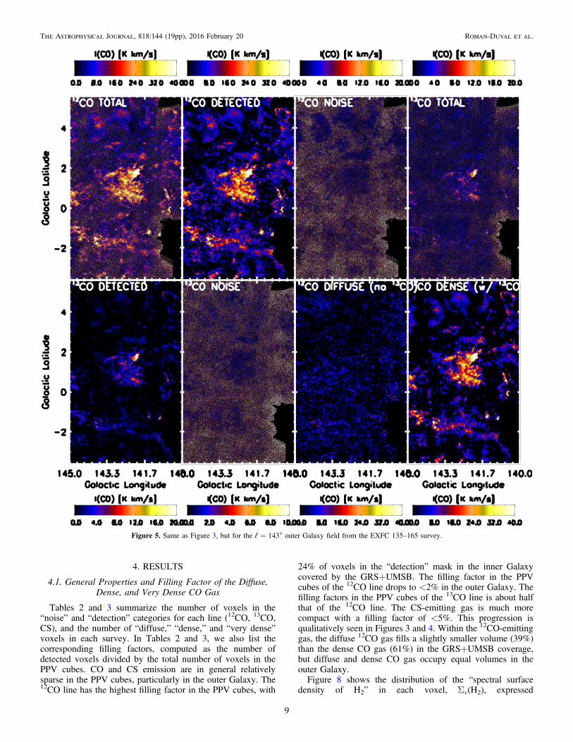
Tables 2 and 3 summarize the number of voxels in the“noise” and “detection” categories for each line (12CO, 13CO,CS), and the number of “diffuse,” “dense,” and “very dense”voxels in each survey. In Tables 2 and 3, we also list thecorresponding filling factors, computed as the number ofdetected voxels divided by the total number of voxels in thePPV cubes. CO and CS emission are in general relativelysparse in the PPV cubes, particularly in the outer Galaxy. The12CO line has the highest filling factor in the PPV cubes, with

24% of voxels in the “detection” mask in the inner Galaxycovered by the GRS+UMSB. The filling factor in the PPVcubes of the 12CO line drops to <2% in the outer Galaxy. Thefilling factors in the PPV cubes of the 13CO line is about halfthat of the 12CO line. The CS-emitting gas is much morecompact with a filling factor of <5%. This progression isqualitatively seen in Figures 3 and 4. Within the 12CO-emittinggas, the diffuse 12CO gas fills a slightly smaller volume (39%)than the dense CO gas (61%) in the GRS+UMSB coverage,but diffuse and dense CO gas occupy equal volumes in theouter Galaxy.Figure 8 shows the distribution of the “spectral surface

density of H2” in each voxel, vS (H2), expressed

Figure 5. Same as Figure 3, but for the ℓ=143° outer Galaxy field from the EXFC 135–165 survey.

9

The Astrophysical Journal, 818:144 (19pp), 2016 February 20 Roman-Duval et al.

inMe pc−2 (km s−1)−1, for the diffuse, dense, and very densecomponents, in each survey. Spectral surface densitiescorrespond to the surface density of H2 along the line of sightat the velocity of the voxel, per unit velocity. As expected, thedistributions of the diffuse, dense, and very dense componentspeak at increasingly higher spectral surface densities (3, 8, and12Me pc−2 (km s−1)−1, respectively). We note that, in order toobtain the surface density of a parcel of molecular gas, thespectral surface densities need to be multiplied by the velocitywidth of that parcel. Hence, the spectral surface densitiesshown in Figure 8 cannot be directly compared to the typicalsurface densities of GMCs. For comparison however, we alsoshow in Figure 8 the distribution of the spectral surfacedensities in voxels within the GMCs identified in Roman-Duval et al. (2010), which closely resembles the spectralsurface density distribution of the very dense gas, peaking at

vS (H2) = 15Me pc−2 and exhibiting a long tail to high spectralsurface densities.

The distribution of the H2 spectral surface density in eachvoxel in the EXFC survey appears wider. However, thedifference in the width of the distribution between the GRS+UMSB and EXFC is most likely due to the difference inmeasurement errors ( 12s ) at the original resolution of the data(typically 12s ∼ 2 K per native (22 5×22 5×0.13 km s−1)

voxel in EXFC, compared to 12s ∼ 0.24 to 0.5 K per native(1′×1′×0.3 km s−1) voxel in the GRS+UMSB).

4.2. Spatial Distribution of Molecular Gas in the Milky Way:A Face-on View

With the knowledge of the location (distance and coordi-nates), luminosity, and mass of each voxel, we have produced aface-on map of the Galactic distribution of 12CO-emittingmolecular gas, separating the diffuse (12CO-bright, 13CO-dark)and dense (12CO-bright, 13CO-bright) CO components. Themaps were obtained by summing in each 100 pc×100 pcpixel the masses of all voxels located within a pixel, anddividing by the area of that pixel. The resulting face-on mapsare shown in Figure 9. Strikingly, the surface density ofmolecular gas decreases by one to two orders of magnitudebetween Galactocentric radii of 3 and 15 kpc. In both sides ofthe solar circle, the diffuse CO component is smoother andmore uniform than the dense component, which is consistentwith the conclusions of Pety et al. (2013) in M51, who foundthat 50% of the CO luminosity in M51 originatesfrom kiloparsec-scale diffuse emission.The large uncertainties on the distance will undoubtedly

affect the detailed spatial distribution of molecular gas in theface-on maps. These maps should therefore not be used toderive the detailed structure of the Milky Way, but rather aremeant to better conceptualize and visualize the transformationsinvolved, between looking through the Galactic Plane and fromabove the Galactic Plane. In the next section, the radial andvertical distributions of H2 and of the different CO componentsare computed by averaging those maps in bins of Galacto-centric radius and vertical height above the plane.

4.3. Radial Distribution of the 12CO, 13CO, and CSAverage Galactic Integrated Intensities

We first examine the distribution of 12CO, 13CO, and CSaverage Galactic integrated intensities Igal with Galactocentricradius Rgal. Here, average Galactic integrated intensitycorresponds to the total luminosity in a Galactocentric radius

Figure 6. Same as Figure 3, but for the ℓ=86° field from the EXFC 55–100 survey (inner and outer Galaxy).

Table 4Definition of the Diffuse, Dense, and Very Dense Components

12CO 1-0 13CO 1-0 CS 2-1 vS (H2)(Me

pc−2 (km s−1)−1)

Diffuse Detected Undetected Undetected <10Dense Detected Detected Undetected >10Very dense Detected Detected Detected >20

Note. vS (H2) is the approximate threshold spectral surface density between thedifferent regimes “diffuse,” “dense,” and “very dense.”

10

The Astrophysical Journal, 818:144 (19pp), 2016 February 20 Roman-Duval et al.

Figure 7. Relation between the 12CO luminosity of a voxel and its H2 mass at agalactocentric radius Rgal = 5.6 kpc (top) and Rgal = 11 kpc (middle), using thecombined data sets (GRS+UMSB, EXFC 55–100 and 135–165). The relationsare derived from voxels with 13CO emission >2 13s only. The slope of therelation is indicated in the legend, and corresponds to XCO = 1.9 1020´ cm−2

(K km s−1)−1 s at Rgal = 5.6 kpc , and XCO = 3.7 1020´ cm−2 (K km s−1)−1

at Rgal = 11 kpc. The bottom panel shows the XCO factor as a function ofGalactocentric radius Rgal.

Figure 8. Distribution of the H2 spectral surface density in each voxel (surfacedensity along the line of sight per unit velocity, expressedin Me pc−2 (km s−1)−1) in each survey. The top panel corresponds to theinner Galaxy with the GRS+USMB surveys. The middle panel includes datafrom the EXFC 135–165 survey (outer Galaxy), and the bottom panels showsdata from the EXFC 55–100 survey (inner and outer Galaxy). The diffuse(detected in 12CO, undetected in 13CO), dense (detected in 12CO and 13CO),and very dense (detected in 12CO, 13CO, and CS, inner Galaxy only)components are indicated by red, green, and blue lines, respectively. The blackline corresponds to the total contribution of these three components. Thedistribution of spectral surface densities in voxels located within giantmolecular clouds identified in the GRS by Roman-Duval et al. (2010) isshown in magenta. In the inner Galaxy, the field where CS observations wereobtained only covered 2 deg2, and therefore corresponds to a number of voxelstoo small to be seen in the histogram. We thus plot the number of voxels in this“very dense” category multiplied by ∼200 so that it can be clearly seen in thehistogram plots.

11

The Astrophysical Journal, 818:144 (19pp), 2016 February 20 Roman-Duval et al.

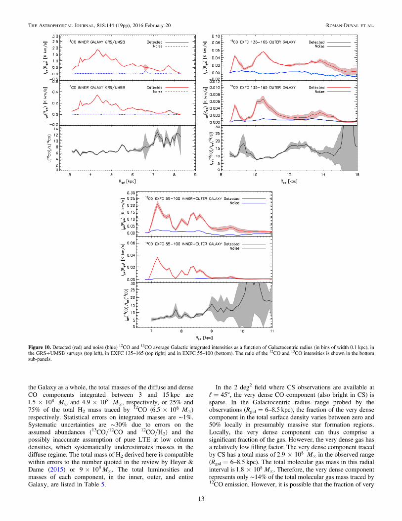
bin, divided by the surface area covered by the survey in thatbin, projected onto the Galactic disk. Igal is therefore theintegrated intensity as seen from above the plane, averagedover radial bins of width 0.1 kpc, and is equivalent to theintegrated intensity measurements for extragalactic surveys offace-on galaxies. In the inner Galaxy, the average Galacticintegrated intensities are obtained for each Monte Carlorealization of distances separately. We then average the trendsof I Rgal gal( ) versus Rgal over all 10 realizations, and we includethe standard deviation between realizations in the final errorestimation. As an additional check that our detection algorithmpicks up all the low-level extended emission, we also computethe average Galactic integrated intensities of the voxels withnon-detections (“noise voxels”) using a similar procedure. Theresulting average Galactic integrated intensities for 12CO and13CO, as well as their ratio, are plotted as a function ofgalactocentric radius in Figure 10 for each survey. The averageGalactic integrated intensity in the CS 2-1 line is plotted versusRgal in Figure 11. Of course, these trends are representative ofthe gas seen within the coverage of the surveys.

To compute the total error on I Rgal gal( ), indicated at 1σ bythe thickness of the curves in Figures 10 and 11, we sum inquadrature the different sources of errors. These sourcesinclude errors on the near and far distance estimation due tonon-circular motions, for the inner Galaxy, the standarddeviation between Monte-Carlo distance realizations, and theresiduals from the average Galactic integrated intensity of“noise” voxels. For a given voxel, the error on its luminosityincurred by the error on its distance is given by L L d d2d d= ,where d and dd are the distance of the voxel and its error and Lits luminosity. The error on the total luminosity in aGalactocentric radius bin is the quadratic sum of the errorson the luminosities of all the voxels included in that bin. Wenote that the standard deviation between near/far distancerealizations in the inner Galaxy is negligible compared to theother sources of errors.

The average Galactic integrated intensity of 12CO and 13COdecreases by one to two orders of magnitude between Rgal ∼3 kpc and Rgal ∼ 15 kpc. I Rgal gal( ) for 12CO and 13CO trackeach other closely throughout the Galactic plane, with anapproximately constant ratio of 5 out to Rgal = 6.5 kpc. The12CO/13CO integrated intensity ratio increases to 10–12 in thesolar neighborhood, although the errors are larger in this case,

and remains between 10 and 20 in the outer Galaxy, out toRgal = 14 kpc. The 12CO/13CO integrated intensity ratioappears to be anti-correlated with I Rgal gal( ), or in other words,with average Galactic surface density of CO-bright moleculargas. This factor-of-two increase in the 12CO/13CO luminosityratio between 3 kpc and the solar neighborhood has previouslybeen observed by Liszt et al. (1984). They interpret it as being aresult of the volume density decreasing away from the Galacticcenter, which would be consistent with the decreasing starformation rate and resulting cloud temperatures seen in Roman-Duval et al. (2010). Additionally, the radial trend in the12CO/13CO luminosity ratio could be explained by thedecrease in the fraction of dense gas with decreasing surfacedensity (and increasing Galactocentric radius), and the13CO/12CO abundance gradient observed in Milam et al.(2005), which varies between 50 at Rgal = 5 kpc and 100 atRgal = 15 kpc and could be consistent with the variations inluminosity ratio. Other possible effects that could explain thevariations in the 12CO/13CO integrated intensity or luminosityratio include more sub-thermally excited 13CO in the outerGalaxy.

4.4. Radial Distribution of the Diffuse, Dense,and Very Dense CO Components

Similarly, we derive the average Galactic H2 surface densityRHgal 2 gal( )( )S in the diffuse extended, dense, and very dense

components, by summing the masses of all voxels in each COcomponent in Galactocentric radius bins of width 0.1 kpc, anddividing by the surface area of each survey projected on theGalactic Plane. The resulting radial distributions of the threeCO gas components are shown in linear space separately foreach survey in Figure 12 and in logarithmic space combiningall data sets in Figure 13. As for the 12CO and 13CO averageGalactic integrated intensity computation, all relevant sourcesof errors are included in the final error budget.In the inner Galaxy, the dense component dominates in

mass. The mass fraction of dense gas decreases from 90% atRgal = 4 kpc to 50% in the solar neighborhood. In the outerGalaxy, the mass fraction of dense gas varies between 40% and80%, and is anti-correlated with surface density.Assuming that the Galaxy is roughly axisymmetric and that

the radial trends observed in our surveys are representative of

Figure 9.Map of the total (left), dense (middle, detected in 12CO and 13CO), and diffuse (right, detected in 12CO, undetected in 13CO) average Galactic surface densityof molecular gas in the Milky Way. The coverage of the two surveys is indicated by the gray/white contrast.

12

The Astrophysical Journal, 818:144 (19pp), 2016 February 20 Roman-Duval et al.

the Galaxy as a whole, the total masses of the diffuse and denseCO components integrated between 3 and 15 kpc are1.5 108´ Me and 4.9 108´ Me, respectively, or 25% and75% of the total H2 mass traced by 12CO (6.5 108´ Me)respectively. Statistical errors on integrated masses are ∼1%.Systematic uncertainties are ∼30% due to errors on theassumed abundances (13CO/12CO and 12CO/H2) and thepossibly inaccurate assumption of pure LTE at low columndensities, which systematically underestimates masses in thediffuse regime. The total mass of H2 derived here is compatiblewithin errors to the number quoted in the review by Heyer &Dame (2015) or 9×108Me. The total luminosities andmasses of each component, in the inner, outer, and entireGalaxy, are listed in Table 5.

In the 2 deg2 field where CS observations are available atℓ=45°, the very dense CO component (also bright in CS) issparse. In the Galactocentric radius range probed by theobservations (Rgal = 6–8.5 kpc), the fraction of the very densecomponent in the total surface density varies between zero and50% locally in presumably massive star formation regions.Locally, the very dense component can thus comprise asignificant fraction of the gas. However, the very dense gas hasa relatively low filling factor. The very dense component tracedby CS has a total mass of 2.9 108´ Me in the observed range(Rgal = 6–8.5 kpc). The total molecular gas mass in this radialinterval is 1.8 108´ Me. Therefore, the very dense componentrepresents only ∼14% of the total molecular gas mass traced by12CO emission. However, it is possible that the fraction of very

Figure 10. Detected (red) and noise (blue) 12CO and 13CO average Galactic integrated intensities as a function of Galactocentric radius (in bins of width 0.1 kpc), inthe GRS+UMSB surveys (top left), in EXFC 135–165 (top right) and in EXFC 55–100 (bottom). The ratio of the 12CO and 13CO intensities is shown in the bottomsub-panels.

13

The Astrophysical Journal, 818:144 (19pp), 2016 February 20 Roman-Duval et al.

dense gas traced by CS be higher closer to the center of theGalaxy.

As a comparison, Battisti & Heyer (2014) found that the verydense component of molecular clouds, as traced by mm dustcontinuum emission, comprises ∼10% of the mass of molecularclouds identified with the CPROPS detection algorithm(Rosolowsky & Leroy 2006). In Section 5.1, we show thatabout 15% of the total molecular gas mass traced by 12CO inthe Milky Way resides in such GMCs, and so the very densegas fraction determined in Battisti & Heyer (2014) wouldrepresent about 1.5% of the total H2 mass traced by 12CO,which is slightly lower than the very dense gas fractionderived here.

4.5. Anti-correlation between Diffuse CO gas and GalacticSurface Density of Molecular Gas

Figure 12 suggests that the fraction of dense CO gas iscorrelated with the Galactic surface density of molecular gas(traced by 12CO). We plot in the top panel of Figure 14 therelation between the mass fraction of dense CO gas and theGalactic molecular gas surface density, averaged in 100 pcwide pixels as seen from above the Galaxy (see Figure 9). Atlow molecular surface densities ( 10gal

100 pc 5S < Me kpc−2), thefraction of dense gas is low ( fDG < 20%–30%). The dense gasfraction increases when the disk’s molecular gas surfacedensity increases, and reaches 80%–90% at high surfacedensities of 107Me kpc−2. A linear fit in log–log space to the

gal100 pcS —fDG relation yields fDG = 0.02 gal

0.24 0.01S .The relation between Galactic surface density of H2 and the

fraction of very dense gas (traced by CS emission), fVDG, isshown in the bottom panel of Figure 14. The mass fraction ofvery dense gas (presumably star-forming) also increases withincreasing disk surface density, from fVDG = 1% at gal

100 pcS = a

few 105Me kpc−2, up to fVDG = 30% at gal100 pcS =

107Me kpc−2. A linear fit in log–log space yieldsfVDG = 3.7 10 7´ -

gal0.8 0.1S .

4.6. Vertical Distribution of CO Gas in the Milky Way

We derive the vertical distribution (i.e., perpendicular to theGalactic plane) of the total, diffuse, dense, and very dense COcomponents. Knowing the distance of each voxel, its height

above the plane z was computed as z d btan( )= . We thensummed the masses of all voxels in vertical height bins ofwidth 5 pc and galactocentric radius bins of width 1 kpc,divided by the surface areas on the Galactic Plane covered byeach survey in those radial bins, and divided by the bin width(5 pc) to obtain the average molecular gas density H2( )r

Figure 11. Detected (red) and noise (blue) CS average Galactic integratedintensities as a function of Galactocentric radius (in bins of width 0.1 kpc), inthe 2 deg2 field of the GRS.

Figure 12. Average Galactic H2 surface densities of the diffuse (red, detectedin 12CO, undetected in 13CO), dense (green, detected in 12CO and 13CO), andvery dense (blue, detected in 12CO, 13CO, and CS) components averaged inbins of width 0.1 kpc, as a function of Galactocentric radius in the GRS+UMSB (inner Galaxy only, top), in the EXFC 135–165 survey (outer Galaxyonly, middle), and in the EXFC 55–100 survey (inner and outer Galaxy,bottom). In the inner Milky Way covered by the GRS, the pink filled curveindicates the surface density of H2 in molecular clouds identified with a clumpfinding algorithm in Roman-Duval et al. (2010).

14

The Astrophysical Journal, 818:144 (19pp), 2016 February 20 Roman-Duval et al.

(inMe pc−3) as a function of z and Rgal for the overall CO gas,as well as the diffuse, dense, and very dense CO gascomponents. In the inner Galaxy, the vertical profile of themolecular gas density was derived for each Monte Carlorealization and then averaged over all realizations. Theresulting vertical profiles are shown in Figure 15. The profilesare fitted with Gaussians, and the resulting centroid andFWHM values are plotted as a function of Galactocentricradius in Figure 16.

The total vertical profile of molecular gas in the inner Galaxyis well described by a Gaussian function with a FWHM of

∼110 pc. As seen in the radial distribution of diffuse and denseCO gas, the dense CO component dominates the inner Galaxyin mass. The profile of the diffuse component in theinner Galaxy is also Gaussian, but with a larger FWHM of130–200 pc. In contrast, the very dense component isconcentrated in the Galactic plane, with a non-Gaussian,double-peaked profile of FWHM ∼ 50 pc.In the outer Galaxy, the molecular disk is more warped, with

a centroid increasing from a few parsecs at the solar circle, upto 150 pc at Rgal = 14 kpc. The molecular disk is wider than inthe inner Galaxy, with FWHM varying between 110 and 300pc. The vertical profiles have multiple peaks and are thus notwell fit by a Gaussian. The FWHM shown in Figure 16 thusrepresents a gross approximation of the profile width. In theouter Galaxy, the diffuse CO component has a similar mass asthe dense CO gas, but their vertical profiles differ significantly.The vertical profile of the diffuse CO gas appears smoother andwider than the profile of the dense CO gas.In both the inner and outer Galaxy, these results are

consistent with previous estimates of the thickness and mid-plane displacement summarized by Heyer & Dame (2015). Thelarger vertical extent of the diffuse CO component suggests thatit originates from a thick disk, which has already beensuggested in the Milky Way by Dame & Thaddeus (1994), andin M51 by Pety et al. (2013).

5. DISCUSSION, LIMITATIONS, AND IMPLICATIONS

5.1. Comparison to the Radial and Vertical Distributionof Molecular Gas Identified as Part of GMCs

Studies of the properties and distribution of molecular gas ingalaxies commonly resort to a cloud identification algorithm,such as CLUMPFIND (Williams et al. 1994) or dendrogram(Rosolowsky et al. 2008) algorithms. These procedures allow

Figure 13. Average Galactic H2 surface densities of the diffuse (red, detected in12CO, undetected in 13CO) and dense (green, detected in 12CO and 13CO) components

as a function of Galactocentric radius (in bins of width 0.1 kpc), in logarithmic scale, combining all data sets. In the inner Galaxy, the pink line indicates the surfacedensity of H2 in molecular clouds identified in Roman-Duval et al. (2010).

Table 5Total Luminosity and Molecular Mass in the Milky Way in the

Diffuse and Dense Components Traced by 12CO

Inner Outer Total

L(12CO)

Diffuse 2.0 101´ 4.0 2.4 101´Dense 1.1 102´ 3.8 1.1 102´

Very dense 4.8 K 4.8Total 1.3 102´ 7.7 1.4 102´

M(H2)

Diffuse 9.3 107´ 6.0 107´ 1.5 108´Dense 4.6 108´ 3.9 107´ 4.9 108´

Very dense 2.9 107´ K 2.9 107´Total 5.5 108´ 9.9 107´ 6.5 108´

Note. Luminosities are given in units of K km s−1 kpc2. Masses are given inMe. Statistical errors on integrated luminosities and masses are ∼1%.Systematic uncertainties are ∼30% due to uncertainties on abundances(13CO/12CO and 12CO/H2) and the possibly non-applicable assumption ofLTE in the diffuse regime, which systematically underestimates masses at lowcolumn densities.

15

The Astrophysical Journal, 818:144 (19pp), 2016 February 20 Roman-Duval et al.

catalogs of discrete objects and associated properties to bederived, including a distance derivation, which cannot beunambiguously determined in the inner Galaxy on a per voxelbasis. However, it is not clear what fraction of the total COemission this type of algorithm picks up. In the left panel ofFigure 12, we show the radial distribution of H2 withinmolecular clouds identified in Roman-Duval et al. (2010),within the same survey coverage. The molecular gas traced byclouds identified with CLUMPFIND in Roman-Duval et al.(2010) represents a small fraction of the total molecular gas inthe inner Milky Way. The total mass of molecular gas in GMCsin the UMSB+GRS coverage is 4.6 107´ Me, while in thisanalysis we derive a total molecular gas mass of 3.4 108´ Me

within the same coverage (not to be confused with the massextrapolated to the entire galaxy in Section 4.4, or6.5 108´ Me). Thus, only ∼14% of the molecular gas massin the Milky Way was identified within GMCs in the innerMilky Way based on their 13CO emission. This number issignificantly smaller than the 40% quoted in Solomon & Rivolo(1989) and Williams & McKee (1997). However, these studies

identified the GMCs in the 12CO cubes, whereas Roman-Duvalet al. (2010) identified CO clouds in the GRS 13CO cubes. It iswell known (e.g., Goldsmith et al. 2008; Heyer et al. 2009, andthis work) that 12CO emission is more (approximately a factorof two) spatially extended than its 13CO counterpart, and so it isnot surprising that the mass fraction of CO gas in 12CO-identified GMCs is larger than the mass fraction of CO gas in13CO-identified GMCs. While the Milky Way is more confusedthan external galaxies, this suggests that studies of moleculargas relying on molecular cloud identification algorithms maybe missing the majority of the molecular gas mass.

5.2. Nature of the “Diffuse,” “Dense,” and “Very Dense” Gas

We identify the “diffuse” gas reported here effectively basedon its high T T12 13 ratio, which implies a low optical depth, andtherefore a low surface density. In Section 3.2, we estimate thatthe spectral surface density transition between the gascomponents we classify as “dense” and “diffuse” is about10Me pc−2 (km s−1)−1, corresponding to surface densities of25–50Me pc−2 for typical line widths. In this context, weinterpret the “diffuse” gas as being of low surface density, andlikely gravitationally unbound and unable to form stars, whilethe “dense” gas corresponds to a gas component, the physicalproperties (density, surface density, viral parameter) of whichare similar to those in the classical sense of molecular clouds.The “diffuse” gas is observed both in the form of isolatedextended structures, but also in the envelopes of dense gas.There are, however, other effects that can induce high T T12 13

ratios. In particular, the wings of optically thick 12CO emissionfrom dense clouds can be broader than the corresponding 13COline while emanating from the same dense gas. In this study,the emission corresponding to those optically thick 12CO linewings would be included in the “diffuse” component. Thus, wemay be overestimating the emission and mass of truly diffusegas, while underestimating the amount of truly dense gas. Wecannot differentiate the emission from truly diffuse gas fromthe dense gas emission in the opacity-broadened wings of the12CO line, because we do not segment the emission into clouds(there are no GMCs in our study). However, we observe that40% of the gas mass classified here as “diffuse” in the outerGalaxy is located in sight-lines toward which no dense gas isdetected. This implies that at least 40% of the “diffuse” gasmass fraction reported here in the outer Galaxy corresponds totruly diffuse gas. In the inner Milky Way, the “diffuse” gasmass fraction with no associated dense component is 15% inthe EXFC 55–100 coverage, and 5% in the GRS+UMSBcoverage. However, these numbers are not meaningful in theinner Milky Way because most line of sights exhibit more thanone CO line detection.To evaluate more quantitatively the fraction of gas that we

report to be “diffuse,” but actually corresponds to the opacity-broadened line wings of dense gas in sight-lines where bothdiffuse and dense gas are detected, we compute the centroidvelocity maps of our “diffuse” and “dense” components. Forsight-lines in which both “diffuse” and “dense” gas aredetected, we then compute, for each survey, the cumulativemass distribution of “diffuse” gas as a function of thedifference in centroid velocity between that “diffuse” and the“dense” gas along the same line of sight (Figure 17). If the highT T12 13 ratio gas that we classify as “diffuse” actuallycorresponds to the optically thick line wings of 12CO, thenone would expect the centroid velocity of this component to be

Figure 14. Relation between dense (top, detected in 12CO and 13CO) and verydense (bottom, detected in 12CO, 13CO, and CS) molecular gas fraction andaverage Galactic surface density of molecular gas, derived from the combineddata sets. The gray scale indicates the density of points, while the pink/greendots show the binned average. The errors bars correspond to the standarddeviation in each bin.

16

The Astrophysical Journal, 818:144 (19pp), 2016 February 20 Roman-Duval et al.

similar to the centroid velocity of the “dense” gas. In the GRS+UMSB surveys, 90% of the gas we report as “diffuse” has acentroid velocity farther than 5 km s−1 from the centroid of the“dense” gas along the same sight-line. In the EXFC 55–100and EXFC 135–195, 65% and 45% of the gas mass that weclassify as “diffuse” has a centroid velocity farther than5 km s−1 from the centroid of the “dense” gas. The typical linewidth of CO clouds is 5 km s−1, and so Figure 17 implies thatmost of the gas mass classified as “diffuse” in this study does

correspond to truly diffuse gas, and not to emission from theopacity-broadened line wings of the 12CO line.Because of the high critical density of CS emission and because

we detect CS 2-1 emission with T T12 CS < 15, corresponding tospectral surface densities > 20Me pc−2 (km s−1)−1 and surfacedensities >100Me pc−2 for typical line widths, we interpret the“very dense” gas as being relatively compact, gravitationallybound, and star-forming gas. Indeed, Lada et al. (2010) derive a

Figure 15. Vertical distribution of molecular gas traced by CO as a function of Galactocentric radius, with the contributions of the diffuse extended (detected in 12CObut not 13CO) and dense (detected in 12CO and 13CO) components in red and green respectively. The vertical distributions are derived with the combined data sets. inthe inner Galaxy, the very dense component traced by CS emission is shown in blue. The black lines corresponds to the total profiles.

Figure 16. Centroid (top) and FWHM (bottom) of the vertical profiles ofmolecular gas traced by CO as a function of Galactocentric radius, obtainedfrom fitting the vertical profiles shown in Figure 15 to Gaussians. Thecontributions of the diffuse extended and dense components are shown in redand green, respectively. In the inner Galaxy, the very dense component tracedby CS emission is shown in blue. The black curve corresponds to the totalprofile.

Figure 17. Cumulative mass fraction of gas classified as “diffuse” as a functionof the centroid velocity difference between the “diffuse” and “dense” gas,calculated in sight-lines where both “diffuse” and “dense” gas components aredetected. The black, red, and blue curves correspond to the GRS+UMSB,EXFC 55–100, and EXFC 135–195, respectively.

17

The Astrophysical Journal, 818:144 (19pp), 2016 February 20 Roman-Duval et al.

threshold of 120Me pc−2 for star formation to occur, close to the“dense” to “very dense” threshold used here. It is however worthmentioning that Galactic Plane surveys of the CS line with highersensitivity than the GRS (Liszt 1995; Helfer & Blitz 1997) haveshown that every 13CO feature has emission from CS at a level∼1%–2% of the 12CO emission. The densities derived from suchweak emission are consistent with rather diffuse molecular gas(low hundreds cm−3). This is however not the gas we are probinghere with CS emission at the level T T12 CS < 15.

5.3. Variable CO–H2 Conversion Factor

In this work, we compute H2 masses and surface densities invoxels with 12CO and 13CO emission detectable at >2σ underthe assumption of LTE and a constant 12CO/13CO abundance.We derive the (constant) conversion factor between 12COluminosity and H2 mass in this sample of voxels. For voxelswith 13CO emission below 2s (and detected 12CO emission),we assume this same constant CO-to-H2 conversion factorderived in the voxels detected in 13CO (see Section 3.4) tocompute an H2 mass. However, we note that the XCO factor islikely to vary and increase for low surface density gas. This gasis less shielded against the interstellar radiation field, whichaffects CO more strongly than H2. While H2 is well protectedagainst photodissociation above an extinction of A 1V ~ , COrequires values of AV ≈2–3 under solar neighborhoodconditions (see, e.g., Tielens & Hollenbach 1985; Wolfireet al. 1993; Röllig et al. 2007; Glover et al. 2010; Glover &Mac Low 2011; Shetty et al. 2011a, 2011b). Indeedobservations of nearby clouds show strong spatial variationsof XCO (e.g., see Pineda et al. 2008; Lee et al. 2014, for adetailed analysis of the Perseus cloud). The fraction of diffusegas scales linearly with the CO-to-H2 conversion factorassumed. Since the CO-to-H2 conversion factor may besignificantly higher in diffuse gas compared to dense gas, thediffuse gas fraction derived here represents a lower limit. Wenote however that, when averaged over a large enough volumeof the ISM or when focusing on the bulk of the molecular masstraced by CO lines, taking a roughly constant XCO-factor givesacceptable results for solar-metallicity galaxies even whenapplied to the diffuse component (Solomon et al. 1987; Young& Scoville 1991; Liszt et al. 2010).

5.4. Diffuse CO Gas and Star formation

As alluded to in Section 1, there is a debate about theuniversality and slope of the K-S relation in nearby galaxies.Shetty et al. (2013, 2014b) argue in favor of galaxy-to-galaxyvariation. Most, but not all, galaxies in their study portray asub-linear relation between star formation rate surface densityand molecular gas surface density (see also, Blanc et al. 2009;Ford et al. 2013). Shetty et al. (2014a) suggest that a non-linearK-S relation may result from the presence of CO not related todense star-forming clouds, perhaps in a diffuse but pervasivemolecular component. Our analysis confirms that this compo-nent of the ISM exists and contains about 25% of the totalmolecular ISM as traced by CO. If the SFR is linearly related tothe amount of very high density gas, and if the radial trends wefind in this work hold throughout the Galaxy, according toShetty et al. (2014a), the underlying relationship between thestar formation rate surface density and H2 would be super-linear (see their Figure 3). We furthermore note that even in theinner Galaxy, which is clearly dominated by dense molecular

gas, only 14% of molecular gas is associated with knownmolecular clouds as identified in the UMSB+GRS surveys(Roman-Duval et al. 2010). The bulk of this dense gas is foundin a more distributed configuration. Our analysis suggests thatthe star formation process could simply be limited by theavailability of such high-density gas at any given time.

6. CONCLUSION

We have examined the spatial distribution of three CO-emitting gas components in the Milky Way, a diffusecomponent traced by 12CO, but dark in 13CO, a densecomponent traced by both 12CO and 13CO, and, in the innerGalaxy only, a very dense component bright in 12CO, 13CO,and CS rotational emission. We have developed a robustalgorithm to determine whether a voxel has significantemission from those tracers. The algorithm first smoothes thespectral cubes so that the S/N of the different line tracers areconsistent with each other. A mask is then based on thethresholding (1σ) of the smoothed cubes. The detection masksare eroded and dilated to remove spurious noise peaks, sincethe 1σ threshold only filters out 84% of the noise. Finally, weapply the masks to the original (un-smoothed) spectral cubes.We have demonstrated that our approach accurately identifiesall the low-level CO and CS emission.We have applied this detection algorithm to 12CO, 13CO, and

CS spectral observations of the Milky Way in the GRS, UMSB,and EXFC surveys, and identified voxels with noise, diffuse,dense, or very dense CO emission. With kinematic distances toeach voxel in the survey, we have derived masses andluminosities at every position in the Galaxy for each COcomponent. This allowed us to derive total masses of1.5 108´ Me, 4.9 108´ , and 2.9 107´ Me for the diffuse,dense, and very dense components, respectively. Altogether,the diffuse gas comprises 25% of the total molecular gas mass.The very dense gas represents 14% of the total moleculargas mass.We have also derived the radial mass distributions of the

three CO components. The surface density of molecular gasdecreases by two orders of magnitude between Galactocentricradii of 3 and 15 kpc. The dense CO gas dominates in mass inthe inner Galaxy, with a dense gas fraction ranging from 90%at Rgal = 4 kpc down to 50% at the solar circle. The diffuse anddense gas has similar relative contributions in the outer Galaxy.The very dense gas fraction in the inner Galaxy appears to varyconsiderably with position. Locally in density peaks, the verydense gas fraction can reach 50%. But the spatial distribution ofthe very dense gas is sparse, rendering its global masscontribution very small. Both the dense and very dense gasmass fractions are positively correlated with surface density.The overall radial distribution of CO gas in the Milky Way isconsistent with previous studies based on coarser surveyssummarized in the review article by Heyer & Dame (2015).We have derived the vertical distribution of molecular gas in

the Milky Way as a function of galactocentric radius. In theinner Milky Way, the vertical molecular profiles are nearlyGaussian and dominated by the dense gas, with a FWHM of110 pc. The very dense gas is much more concentrated on theGalactic plane, with a FWHM of ∼50 pc. In the outer Galaxy,the vertical molecular profiles are complex and multi-peaked,and wider than in the inner Milky Way, with FWHM as high as300 pc. The vertical distribution and warp of CO molecular gas

18

The Astrophysical Journal, 818:144 (19pp), 2016 February 20 Roman-Duval et al.

are also consistent with previous studies summarized in Heyer& Dame (2015).

R.S. and R.S.K. acknowledge support from the DeutscheForschungsgemeinschaft (DFG) for funding through the SPP1573 “The Physics of the Interstellar Medium” as well as viaSFB 881 “The Milky Way System” (sub-projects B12, andB8). R.S.K. also receives funding from the European ResearchCouncil under the European Communitys Seventh FrameworkProgram (FP7/2007-2013) via the ERC Advanced Grant“STARLIGHT” (project number 339177).

REFERENCES

Battisti, A. J., & Heyer, M. H. 2014, ApJ, 780, 173Bigiel, F., Leroy, A., Walter, F., et al. 2008, AJ, 136, 2846Blanc, G. A., Heiderman, A., Gebhardt, K., Evans, N. J., II, & Adams, J. 2009,

ApJ, 704, 842Burton, W. B., Liszt, H. S., & Baker, P. L. 1978, ApJL, 219, L67Clemens, D. P. 1985, ApJ, 295, 422Clemens, D. P., Sanders, D. B., Scoville, N. Z., & Solomon, P. M. 1986, ApJS,

60, 297Dame, T. M., & Thaddeus, P. 1994, ApJL, 436, L173Federrath, C. 2013, MNRAS, 436, 3167Ford, G. P., Gear, W. K., Smith, M. W. L., et al. 2013, ApJ, 769, 55Glover, S. C. O., Federrath, C., Mac Low, M., & Klessen, R. S. 2010,

MNRAS, 404, 2Glover, S. C. O., & Mac Low, M.-M. 2011, MNRAS, 412, 337Goldsmith, P. F., Heyer, M., Narayanan, G., et al. 2008, ApJ, 680, 428Heiderman, A., Evans, N. J., II, Allen, L. E., Huard, T., & Heyer, M. 2010,

ApJ, 723, 1019Helfer, T. T., & Blitz, L. 1997, ApJ, 478, 233Heyer, M., & Dame, T. M. 2015, ARA&A, 53, 583Heyer, M., Krawczyk, C., Duval, J., & Jackson, J. M. 2009, ApJ, 699, 1092Jackson, J. M., Bania, T. M., Simon, R., et al. 2002, ApJL, 566, L81Kennicutt, R. C., Jr. 1998, ApJ, 498, 541Klessen, R. S., & Glover, S. C. O. 2014, arXiv:1412.5182Knapp, G. R. 1974, AJ, 79, 527Krumholz, M. R., Dekel, A., & McKee, C. F. 2012, ApJ, 745, 69Lada, C. J., Lombardi, M., & Alves, J. F. 2010, ApJ, 724, 687

Lee, M.-Y., Stanimirović, S., Wolfire, M. G., et al. 2014, ApJ, 784, 80Leroy, A. K., Walter, F., Sandstrom, K., et al. 2013, AJ, 146, 19Liszt, H. S. 1995, ApJ, 442, 163Liszt, H. S., Burton, W. B., & Xiang, D.-L. 1984, A&A, 140, 303Liszt, H. S., Pety, J., & Lucas, R. 2010, A&A, 518, A45Liu, G., Koda, J., Calzetti, D., Fukuhara, M., & Momose, R. 2011, ApJ,

735, 63Mac Low, M.-M., & Klessen, R. S. 2004, RvMP, 76, 125Milam, S. N., Savage, C., Brewster, M. A., Ziurys, L. M., & Wyckoff, S. 2005,

ApJ, 634, 1126Momose, R., Koda, J., Kennicutt, R. C., Jr., et al. 2013, ApJL, 772, L13Neufeld, D. A., Godard, B., Gerin, M., et al. 2015, A&A, 577, A49Pety, J., Schinnerer, E., Leroy, A. K., et al. 2013, ApJ, 779, 43Pineda, J. E., Caselli, P., & Goodman, A. A. 2008, ApJ, 679, 481Rathborne, J. M., Johnson, A. M., Jackson, J. M., Shah, R. Y., & Simon, R.

2009, ApJS, 182, 131Röllig, M., Abel, N. P., Bell, T., et al. 2007, A&A, 467, 187Roman-Duval, J., Jackson, J. M., Heyer, M., et al. 2009, ApJ, 699, 1153Roman-Duval, J., Jackson, J. M., Heyer, M., Rathborne, J., & Simon, R. 2010,

ApJ, 723, 492Rosolowsky, E., & Leroy, A. 2006, PASP, 118, 590Rosolowsky, E. W., Pineda, J. E., Kauffmann, J., & Goodman, A. A. 2008,

ApJ, 679, 1338Salim, D. M., Federrath, C., & Kewley, L. J. 2015, ApJL, 806, L36Sanders, D. B., Clemens, D. P., Scoville, N. Z., & Solomon, P. M. 1986, ApJS,

60, 1Schmidt, M. 1959, ApJ, 129, 243Shetty, R., Clark, P. C., & Klessen, R. S. 2014a, MNRAS, 442, 2208Shetty, R., Glover, S. C., Dullemond, C. P., et al. 2011a, MNRAS, 415, 3253Shetty, R., Glover, S. C., Dullemond, C. P., & Klessen, R. S. 2011b, MNRAS,

412, 1686Shetty, R., Kelly, B. C., & Bigiel, F. 2013, MNRAS, 430, 288Shetty, R., Kelly, B. C., Rahman, N., et al. 2014b, MNRAS, 437, L61Soille, P. 1999, Morphological Image Analysis, Principles and Applications

(2nd ed.; Berlin: Springer)Solomon, P. M., & Rivolo, A. R. 1989, ApJ, 339, 919Solomon, P. M., Rivolo, A. R., Barrett, J., & Yahil, A. 1987, ApJ, 319, 730Stutzki, J. 2014, Astrophysics Source Code Library, ascl:1406.018Tielens, A. G. G. M., & Hollenbach, D. 1985, ApJ, 291, 722Williams, J. P., de Geus, E. J., & Blitz, L. 1994, ApJ, 428, 693Williams, J. P., & McKee, C. F. 1997, ApJ, 476, 166Wolfire, M. G., Hollenbach, D., & Tielens, A. G. G. M. 1993, ApJ, 402, 195Young, J. S., & Scoville, N. Z. 1991, ARA&A, 29, 581

19

The Astrophysical Journal, 818:144 (19pp), 2016 February 20 Roman-Duval et al.