distributed wireless power transfer system for internet-of

2327-4662 (c) 2017 IEEE. Personal use is permitted, but republication/redistribution requires IEEE permission. See http://www.ieee.org/publications_standards/publications/rights/index.html for more information.

This article has been accepted for publication in a future issue of this journal, but has not been fully edited. Content may change prior to final publication. Citation information: DOI 10.1109/JIOT.2018.2790578, IEEE Internet ofThings Journal

1

Distributed Wireless Power Transfer System forInternet-of-Things Devices

Kae Won Choi, Senior Member, IEEE, Arif Abdul Aziz, Dedi Setiawan, Nguyen Minh Tran, Lorenz Ginting, andDong In Kim, Senior Member, IEEE

Abstract—The wireless power transfer via an electro-magnetic(EM) wave enables far-field power transfer for supplying powerto IoT devices. However, the power attenuation of the EM waveleads to low end-to-end power transfer efficiency. In this paper,we provide an analytic and experimental study on the distributedwireless power transfer system as a means to overcome thelow power transfer efficiency. In the distributed wireless powertransfer system, a number of multi-antenna power beacons,which are distributed over space, send out wireless power tocharge IoT devices. Since each power beacon has a separatelocal oscillator and controller, it is very challenging to achievefrequency and phase synchronization among power beacons,which is the prerequisite for optimal distributed beamforming. Inthis paper, we study the performance of the distributed wirelesspower transfer system with or without the frequency and phasesynchronization. Based on the experiment and simulation results,we show that the distributed wireless charging is advantageousin terms of the coverage probability as long as the optimaldistributed beamforming is available in the distributed wirelesspower transfer system.

Index Terms—Wireless power transfer, IoT devices, distributedantenna system, wireless-powered sensor networks, coverageprobability, energy harvesting

I. INTRODUCTION

Recently, the wireless power transfer via an electro-magnetic (EM) wave has gained a lot of attention thanks toits capability of far-field power transmission [1]. Differentlyfrom magnetic wireless power transfer techniques such asinductive coupling and magnetic resonant coupling, the RFenergy transfer technique makes use of a radiative EM waveto convey power through a free space. Therefore, the RFenergy transfer enjoys an advantage of relatively longer energytransfer distance compared to magnetic wireless power transfer[2]. However, the wireless power transfer via an EM wavesuffers from low end-to-end transfer efficiency because ofsevere power attenuation. One viable solution to overcome thisproblem in indoor environment is to use a distributed antennasystem [1], [3]. The multi-antenna system with collocatedantennas can efficiently transfer energy only to a limited areaclose to the antennas. On the other hand, the distributedantennas surrounding the target area can cover the whole area,

The authors are with the School of Information and Communication Engi-neering, Sungkyunkwan University (SKKU), Suwon, Korea (email: [email protected], [email protected], [email protected],[email protected], [email protected], [email protected]).

This work was supported in part by the National Research Founda-tion of Korea (NRF) grant funded by the Korean government (MSIP)(2014R1A5A1011478), and in part by the Basic Science Research Pro-gram through the NRF funded by the Korean government (MSIP) (NRF-2017R1A2B4010285).

eliminating blind spots around which no nearby antenna ispresent.

The distributed wireless power transfer system has been the-oretically studied by some works (e.g., [4]–[7]). The authorsof [4] have proposed simultaneous wireless information andpower transfer (SWIPT) and energy cooperation in a multiple-input single-output (MISO) distributed antenna system. In [5],the authors have studied the resource allocation algorithmfor the distributed antenna-based SWIPT. In [6], the authorshave characterized the achievable rate-energy tradeoff in amulti-user SWIPT system with distributed transmitters. Thework [7] has discussed the research trend and the potentialarchitecture of the distributed version of the massive multiple-input multiple-output (MIMO) technology for SWIPT.

Other than those theoretical works, few experimental re-searches regarding the wireless power transfer with the dis-tributed antennas have been conducted (e.g., [8]–[12]). In [8],the ubiquitous power source with a magnetron and a slottedantenna array has been implemented in a shield room, and amobile phone has been successfully charged with microwavepower everywhere in the room. In [9], the distributed retro-reflective beamforming for the wireless power transfer isexperimentally verified. The work [10] has demonstrated theconstructive and destructive energy aggregation at the powerreceiver. In [11], the distributed medium access control (MAC)protocol for wireless power transfer is proposed. In this MACprotocol, the two-tone energy transfer is suggested to mitigatethe negative effect of the phase mismatch between the signalsfrom multiple energy transmitters. In [12], the authors haveproposed the carrier shift diversity (CSD) for multi-pointwireless power transmission, which assigns slightly differentfrequencies to multiple transmitters.

In this paper, we consider the distributed wireless powertransfer system consisting of multiple separate power beacons,each of which is equipped with multiple transmit antennas.In this system, it is of great importance to perform opti-mal distributed beamforming to maximize the power transferefficiency. The optimal distributed beamforming makes theEM waves from all antennas constructively combined atthe receiver so that the receive power is maximized. Theprerequisite for the optimal distributed beamforming is boththe frequency and phase synchronization. Frequency driftsbetween different power beacons are caused by the imper-fection (i.e., hardware offset) of local oscillators. For optimalbeamforming, frequency drifts should be compensated by afrequency synchronization method, for example, a designatedmaster transmitter can send the reference signal to coordinate



2

the synchronization [13]. For the phase synchronization, eachantenna should transmit a signal conjugate to the channel gainbetween transmit and receive antennas. If an independent con-troller is used in each power beacon, the phase synchronizationis a challenging task. In [13] and [14], a closed-loop feedbackalgorithm is proposed for achieving the phase synchronizationin the distributed antenna system. Although some existingmethods (e.g., [13], [14]) can be used for optimal distributedbeamforming, the realization of both the frequency and phasesynchronization is still very costly and challenging.

In this paper, we provide an analytic and experimental studyof the distributed wireless power transfer with or withoutthe frequency and phase synchronization. We consider threebeamforming schemes: optimal, static, and random beam-forming. The optimal beamforming scheme can be used onlywhen the frequency and phase synchronization is achieved.If the phase synchronization is not available, we can use thestatic beamforming scheme that simply fixes the phases of thetransmit signals. However, this static beamforming can causethe signals to be destructively combined in many places. Thisproblem can be solved by using the random beamforming thatrandomizes the phases of the transmit signals. The focus ofthis paper is not to design the beamforming schemes but toanalyze the performance of them. In this paper, we analyze theaverage receive power when the optimal, static, and randombeamforming schemes are applied between multiple antennaswithin each power beacon or across multiple power beacons.In addition, we analyze the coverage probability, which isdefined as the probability that the receive power is not lessthan a given threshold.

We have built a real-life testbed for the distributed wirelesspower transfer. For implementing the multi-antenna powerbeacon, we have designed and fabricated a phased antennaarray board with 16 transmit paths, each of which consistsof a phase shifter, a variable attenuator, and an amplifier. Inaddition, we have implemented a low power IoT device that iscapable of receiving the radio frequency (RF) wireless power.The IoT device consists of off-the-shelf components such asa rectifier, an energy storage, a voltage regulator, a micro-controller unit (MCU), and an RF transceiver. In the testbed,the power beacons and the IoT device are fully integratedto perform the optimal, static, and random beamforming inreal time. We have conducted extensive experiments to showthe receive power all over the testbed space and the coverageprobabilities when various beamforming schemes are used. Weshow that the analysis on the receive power and the coverageprobability very well agrees with the experimental results. Wealso show that the distributed wireless charging is advanta-geous in terms of the coverage probability in comparison toa single power beacon with multiple collocated antennas, aslong as the optimal distributed beamforming is available.

It is noted that this paper is the extended version of ourprevious conference paper [15]. Compared to the conferencepaper, this paper establishes more elaborated system model(e.g., EM wave propagation model and low power IoT devicemodel), includes detailed discussion on the hardware archi-tectures for distributed wireless power transmitters, providesmore advanced mathematical analysis, and presents extensive

experimental and simulation results.In summary, the contributions of this paper are twofold.• We suggest the optimal, static, and random beamforming

schemes for the distributed wireless power transfer inconsideration of the practical limitation in a hardwarecapability. We provide the analysis for these beamformingschemes in terms of the receive power and the coverageprobability. The existing theoretical works (e.g., [4]–[7])do not consider all of these beamforming schemes sincethey assume the perfect knowledge on the channel stateinformation.

• We present extensive experimental results obtained froma real-life testbed for the multi-antenna distributed wire-less power transfer with the optimal, static, randombeamforming, and verify that the analysis well matcheswith the experimental results. No previous experimentalwork (e.g., [8]–[12]) has conducted such comprehensiveexperiments.

The rest of paper is organized as follows. We presentthe system model for the distributed wireless power transferin Section II. We explain the possible architectures of thedistributed wireless power transfer system, and investigatevarious distributed beamforming schemes in Section III. Thereceive power and the coverage probability are analyzed inSection IV. Section V presents the experimental results, andSection VI concludes the paper.

II. SYSTEM MODEL

A. Distributed Wireless Power Transfer-Based IoT SystemModel

In the proposed model for the distributed wireless powertransfer-based IoT system, multiple power beacons emit an RFwave to wirelessly supply power to an IoT device, as depictedin Fig. 1. We assume that there are K power beacons, eachof which is equipped with N transmit antennas. Hereafter,the kth power beacon and the nth antenna are simply calledbeacon k and antenna n, respectively. Each power beaconcan perform energy beamforming by using multiple transmitantennas to focus an energy beam on the IoT device. Moreover,multiple power beacons can cooperate with each other tooptimally deliver the RF power to the IoT device. The energybeamforming along with the cooperation between the powerbeacons will be discussed in more detail in Section III. In theproposed system model, we consider one IoT device, equippedwith a single antenna for receiving the RF power from thepower beacons.

Each transmit antenna in a power beacon emits an RF signalfor wireless power transfer. Let fc denote the frequency of theRF signal. The RF signal at time t, which is sent by antennan of beacon k, is given by

κk,n(t) = Re[xk,n(t) exp

(j2πfct

)], (1)

where xk,n(t) is the baseband complex transmit signal at timet from antenna n of beacon k. The transmit signal xk,n(t) isdetermined by the distributed beamforming algorithm, whichwill be discussed in Section III. Actually, κk,n(t) in (1) is thevoltage signal at the antenna port. If the antenna impedance



3

Power

Beacon

IoT

Device

Power

Beacon

Power

Beacon

Fig. 1. Distributed wireless power transfer-based IoT system model.

is denoted by Z0 (i.e., usually 50 Ω), the transmit power fromthe port of antenna n of beacon k is

pk,n(t) =|xk,n(t)|2

2Z0. (2)

The complex channel gain from antenna n of beacon k tothe antenna of the IoT device is denoted by hk,n. It is notedthat the complex channel gain is equivalent to the S-parameterbetween the ports of the transmit and receive antennas. We willdiscuss the channel gain modeling in more detail in SectionII-B. The RF signal at the antenna of the IoT device, receivedfrom all antennas of all power beacons, is given by

ν(t) = Re[y(t) exp

(j2πfct

)], (3)

where y(t) is the baseband complex receive signal at time tat the antenna of the IoT device. The receive signal y(t) isgiven by

y(t) =K∑k=1

N∑n=1

hk,nxk,n(t) =K∑k=1

hTk xk(t). (4)

In (4), hk and xk(t) denote the channel gain vector hk =(hk,1, . . . , hk,N )T and the transmit signal vector xk(t) =(xk,1(t), . . . , xk,N (t))T , respectively. The receive power at theantenna port of the IoT device is given by

r(t) =|y(t)|2

2Z0. (5)

The received RF power at the IoT device is rectified to theDC power and is used to power up the IoT device. The IoTdevice model will be discussed in Section II-C.

B. Electro-Magnetic Wave Propagation Model

In this subsection, we explain an EM wave propagationmodel for modeling the channel gain hk,n(t). For doing this,we first give a spatial model for the locations of the antennasof the power beacons and the IoT device. For simplicity, weconfine the spatial model to a two-dimensional plane. Weassume that all antennas are omni-directional dipole antennasthat are vertically positioned at the same elevation in referenceto the ground. Then, the location of each antenna can bedescribed only by a two-dimensional coordinate.

Let us denote by bk the two-dimensional reference coor-dinate of beacon k. The relative coordinate of antenna n ofbeacon k in reference to bk is denoted by ak,n. Then, the

absolute coordinate of antenna n of beacon k is (bk + ak,n).The antennas belong to one power beacon are closely locatedto form an antenna array. Then, the arrangement of the antennaarray (e.g., linear or circular antenna array) is determined byak,n for n = 1, . . . , N . Let us denote by c the coordinateof the antenna of the IoT device. Then, the distance betweenbeacon k and the IoT device is dk = ‖bk − c‖2, and thedistance between antenna n of beacon k and the IoT deviceis dk,n = ‖bk + ak,n − c‖2. We assume that no antennacoupling is occurred between antennas since all the antennasare separated by at least half-wavelength.

Now, we present the modeling of the channel gain fromantenna n of beacon k to the IoT device (i.e., hk,n). Thewavelength of the RF signal with frequency fc in a free spaceis denoted by λ. Then, the channel gain is calculated as

hk,n =√L

(d

dk,n

)α2√

gtgr exp

(j2π

dk,nλ

)=√

Υd−α

2

k,n exp

(j2π

dk,nλ

),

(6)

where d is the reference distance for the path loss, L isthe attenuation at the reference distance, α is the path lossexponent, gt is the transmit antenna gain, gr is the receiveantenna gain, and Υ = Ldαgtgr. If we use the Friis equationfor the path loss, we have α = 2, L = 1, and d = λ/(4π).

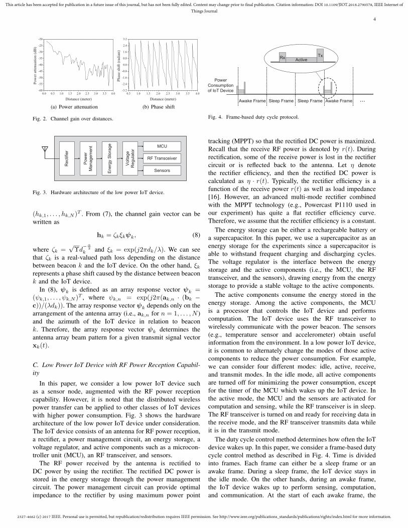
In this paper, we use empirically-obtained values for theparameters Υ and α in (6). To obtain the parameters and tovalidate the channel gain model in (6), we have conductedchannel gain experiments as shown in Fig. 2. In this exper-iment, two dipole antennas with a 3 dBi gain are separatelyplaced by a given distance, and the S-parameter (i.e., S21)between those antennas is measured by a network analyzer. InFig. 2, we show the power attenuation (i.e., 10 log10 |hk,n|2 =10 log10 Υ−α·10 log10 dk,n) and the phase shift (i.e., ∠hk,n =2πdk,n/λ) according to the distance. We can observe that thephase is shifted by 2π for every full wavelength (i.e., 0.32 mfor fc = 920 MHz), as modeled in (6). On the other hand,the power attenuation shows irregularity because of the indoormulti-path environment. This irregularity is not described by(6) since we assume that only a direct line-of-sight (LOS)path exists in (6) for simplicity. However, the channel gainmodel (6) still well describes the general attenuation trends.1

By regression, we have found the empirical parameters for thechannel gain model as Υ = 4.393× 10−4 and α = 2.051.

Multiple antennas equipped in one power beacon form anantenna array that is capable of beamforming. Let us assumethat the IoT device is located within the far-field region of theantenna array of each power beacon. Under this assumption,we can approximate (6) as

hk,n =√

Υd−α

2

k exp

(j2π

dkλ

)exp

(j2π

ak,n · (bk − c)

λdk

),

(7)

where ‘·’ denotes the dot product. Recall that hk denotesthe channel gain vector for power beacon k such that hk =

1For the narrowband signal here, the multi-path channel can be modeledin (6) with a relatively large α > 2.



4

0.0 0.5 1.0 1.5 2.0 2.5 3.0 3.5 4.0-60

-55

-50

-45

-40

-35

-30

-25

-20

P

ow

er

att

en

uati

on

(d

B)

Distance (meter)

(a) Power attenuation

0.5 1.0 1.5 2.0 2.5 3.0 3.5 4.0-3.2

-2.4

-1.6

-0.8

0.0

0.8

1.6

2.4

3.2

Ph

ase

sh

ift

(rad

ian

)

Distance (meter)

(b) Phase shift

Fig. 2. Channel gain over distances.

Re

ctifier

Sensors

RF Transceiver

MCU

Ene

rgy S

tora

ge

Volta

ge

Re

gu

lato

r

Pow

er

Ma

nag

em

en

t

Fig. 3. Hardware architecture of the low power IoT device.

(hk,1, . . . , hk,N )T . From (7), the channel gain vector can bewritten as

hk = ζkξkψk, (8)

where ζk =√

Υd−α

2

k and ξk = exp(j2πdk/λ). We can seethat ζk is a real-valued path loss depending on the distancebetween beacon k and the IoT device. On the other hand, ξkrepresents a phase shift caused by the distance between beaconk and the IoT device.

In (8), ψk is defined as an array response vector ψk =(ψk,1, . . . , ψk,N )T , where ψk,n = exp(j2π(ak,n · (bk −c))/(λdk)). The array response vector ψk depends only on thearrangement of the antenna array (i.e., ak,n for n = 1, . . . , N )and the azimuth of the IoT device in relation to beaconk. Therefore, the array response vector ψk determines theantenna array beam pattern for a given transmit signal vectorxk(t).

C. Low Power IoT Device with RF Power Reception Capabil-ity

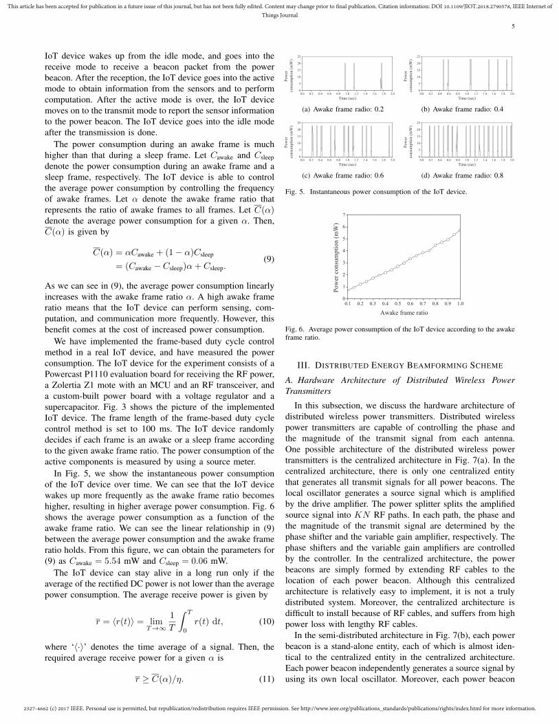
In this paper, we consider a low power IoT device suchas a sensor node, augmented with the RF power receptioncapability. However, it is noted that the distributed wirelesspower transfer can be applied to other classes of IoT deviceswith higher power consumption. Fig. 3 shows the hardwarearchitecture of the low power IoT device under consideration.The IoT device consists of an antenna for RF power reception,a rectifier, a power management circuit, an energy storage, avoltage regulator, and active components such as a microcon-troller unit (MCU), an RF transceiver, and sensors.

The RF power received by the antenna is rectified toDC power by using the rectifier. The rectified DC power isstored in the energy storage through the power managementcircuit. The power management circuit can provide optimalimpedance to the rectifier by using maximum power point

Power

Consumption

of IoT Device

RxActive

Tx

Awake Frame Sleep Frame Sleep Frame Awake Frame

Fig. 4. Frame-based duty cycle protocol.

tracking (MPPT) so that the rectified DC power is maximized.Recall that the receive RF power is denoted by r(t). Duringrectification, some of the receive power is lost in the rectifiercircuit or is reflected back to the antenna. Let η denotethe rectifier efficiency, and then the rectified DC power iscalculated as η · r(t). Typically, the rectifier efficiency is afunction of the receive power r(t) as well as load impedance[16]. However, an advanced multi-mode rectifier combinedwith the MPPT technology (e.g., Powercast P1110 used inour experiment) has quite a flat rectifier efficiency curve.Therefore, we assume that the rectifier efficiency is a constant.

The energy storage can be either a rechargeable battery ora supercapacitor. In this paper, we use a supercapacitor as anenergy storage for the experiments since a supercapacitor isable to withstand frequent charging and discharging cycles.The voltage regulator is the interface between the energystorage and the active components (i.e., the MCU, the RFtransceiver, and the sensors), drawing energy from the energystorage to provide a stable voltage to the active components.

The active components consume the energy stored in theenergy storage. Among the active components, the MCUis a processor that controls the IoT device and performscomputation. The IoT device uses the RF transceiver towirelessly communicate with the power beacon. The sensors(e.g., temperature sensor and accelerometer) obtain usefulinformation from the environment. In a low power IoT device,it is common to alternately change the modes of those activecomponents to reduce the power consumption. For example,we can consider four different modes: idle, active, receive,and transmit modes. In the idle mode, all active componentsare turned off for minimizing the power consumption, exceptfor the timer of the MCU which wakes up the IoT device. Inthe active mode, the MCU and the sensors are activated forcomputation and sensing, while the RF transceiver is in sleep.The RF transceiver is turned on and ready for receiving data inthe receive mode, and the RF transceiver transmits data whileit is in the transmit mode.

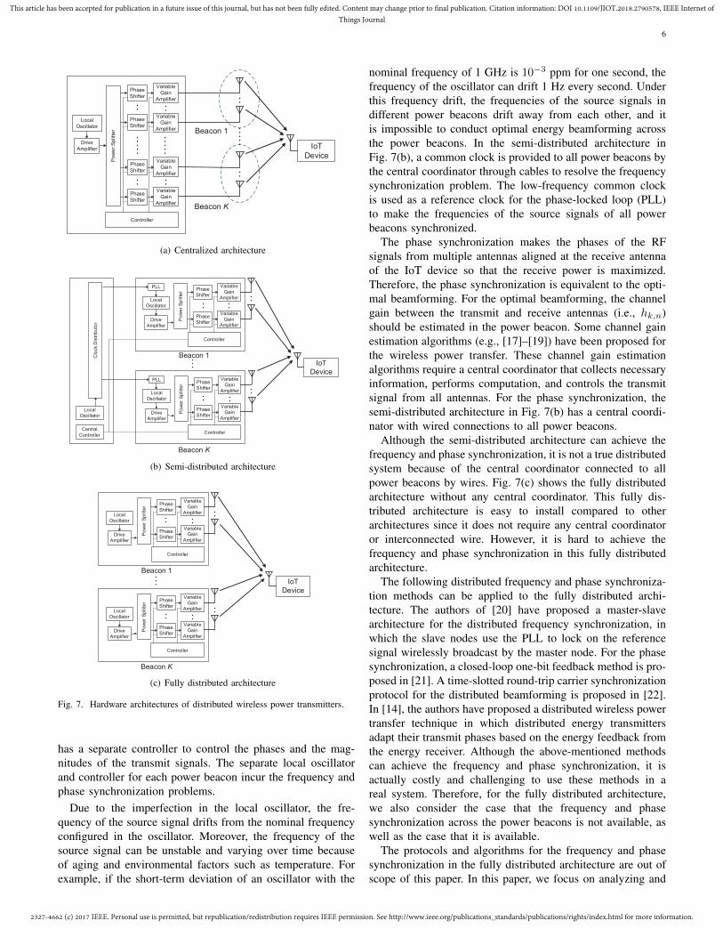
The duty cycle control method determines how often the IoTdevice wakes up. In this paper, we consider a frame-based dutycycle control method as described in Fig. 4. Time is dividedinto frames. Each frame can either be a sleep frame or anawake frame. During a sleep frame, the IoT device stays inthe idle mode. On the other hands, during an awake frame,the IoT device wakes up to perform sensing, computation,and communication. At the start of each awake frame, the



5

IoT device wakes up from the idle mode, and goes into thereceive mode to receive a beacon packet from the powerbeacon. After the reception, the IoT device goes into the activemode to obtain information from the sensors and to performcomputation. After the active mode is over, the IoT devicemoves on to the transmit mode to report the sensor informationto the power beacon. The IoT device goes into the idle modeafter the transmission is done.

The power consumption during an awake frame is muchhigher than that during a sleep frame. Let Cawake and Csleepdenote the power consumption during an awake frame and asleep frame, respectively. The IoT device is able to controlthe average power consumption by controlling the frequencyof awake frames. Let α denote the awake frame ratio thatrepresents the ratio of awake frames to all frames. Let C(α)denote the average power consumption for a given α. Then,C(α) is given by

C(α) = αCawake + (1− α)Csleep

= (Cawake − Csleep)α+ Csleep.(9)

As we can see in (9), the average power consumption linearlyincreases with the awake frame ratio α. A high awake frameratio means that the IoT device can perform sensing, com-putation, and communication more frequently. However, thisbenefit comes at the cost of increased power consumption.

We have implemented the frame-based duty cycle controlmethod in a real IoT device, and have measured the powerconsumption. The IoT device for the experiment consists of aPowercast P1110 evaluation board for receiving the RF power,a Zolertia Z1 mote with an MCU and an RF transceiver, anda custom-built power board with a voltage regulator and asupercapacitor. Fig. 3 shows the picture of the implementedIoT device. The frame length of the frame-based duty cyclecontrol method is set to 100 ms. The IoT device randomlydecides if each frame is an awake or a sleep frame accordingto the given awake frame ratio. The power consumption of theactive components is measured by using a source meter.

In Fig. 5, we show the instantaneous power consumptionof the IoT device over time. We can see that the IoT devicewakes up more frequently as the awake frame ratio becomeshigher, resulting in higher average power consumption. Fig. 6shows the average power consumption as a function of theawake frame ratio. We can see the linear relationship in (9)between the average power consumption and the awake frameratio holds. From this figure, we can obtain the parameters for(9) as Cawake = 5.54 mW and Csleep = 0.06 mW.

The IoT device can stay alive in a long run only if theaverage of the rectified DC power is not lower than the averagepower consumption. The average receive power is given by

r = 〈r(t)〉 = limT→∞

1

T

∫ T

0

r(t) dt, (10)

where ‘〈·〉’ denotes the time average of a signal. Then, therequired average receive power for a given α is

r ≥ C(α)/η. (11)

0.0 0.2 0.4 0.6 0.8 1.0 1.2 1.4 1.6 1.8 2.00

5

10

15

20

25

Po

wer

co

nsu

mp

tio

n (

mW

)

Time (sec)

(a) Awake frame radio: 0.2

0.0 0.2 0.4 0.6 0.8 1.0 1.2 1.4 1.6 1.8 2.00

5

10

15

20

25

Po

wer

co

nsu

mp

tio

n (

mW

)

Time (sec)

(b) Awake frame radio: 0.4

0.0 0.2 0.4 0.6 0.8 1.0 1.2 1.4 1.6 1.8 2.00

5

10

15

20

25

Po

wer

co

nsu

mp

tio

n (

mW

)

Time (sec)

(c) Awake frame radio: 0.6

0.0 0.2 0.4 0.6 0.8 1.0 1.2 1.4 1.6 1.8 2.00

5

10

15

20

25

Po

wer

co

nsu

mp

tio

n (

mW

)

Time (sec)

(d) Awake frame radio: 0.8

Fig. 5. Instantaneous power consumption of the IoT device.

0.1 0.2 0.3 0.4 0.5 0.6 0.7 0.8 0.9 1.00

1

2

3

4

5

6

7

Po

wer

co

nsu

mp

tio

n (

mW

)

Awake frame ratio

Fig. 6. Average power consumption of the IoT device according to the awakeframe ratio.

III. DISTRIBUTED ENERGY BEAMFORMING SCHEME

A. Hardware Architecture of Distributed Wireless PowerTransmitters

In this subsection, we discuss the hardware architecture ofdistributed wireless power transmitters. Distributed wirelesspower transmitters are capable of controlling the phase andthe magnitude of the transmit signal from each antenna.One possible architecture of the distributed wireless powertransmitters is the centralized architecture in Fig. 7(a). In thecentralized architecture, there is only one centralized entitythat generates all transmit signals for all power beacons. Thelocal oscillator generates a source signal which is amplifiedby the drive amplifier. The power splitter splits the amplifiedsource signal into KN RF paths. In each path, the phase andthe magnitude of the transmit signal are determined by thephase shifter and the variable gain amplifier, respectively. Thephase shifters and the variable gain amplifiers are controlledby the controller. In the centralized architecture, the powerbeacons are simply formed by extending RF cables to thelocation of each power beacon. Although this centralizedarchitecture is relatively easy to implement, it is not a trulydistributed system. Moreover, the centralized architecture isdifficult to install because of RF cables, and suffers from highpower loss with lengthy RF cables.

In the semi-distributed architecture in Fig. 7(b), each powerbeacon is a stand-alone entity, each of which is almost iden-tical to the centralized entity in the centralized architecture.Each power beacon independently generates a source signal byusing its own local oscillator. Moreover, each power beacon



6

Po

we

r S

plit

ter

Controller

Variable

Gain

Amplifier

Phase

Shifter

Variable

Gain

Amplifier

Phase

Shifter

Drive

Amplifier

Local

Oscillator

Variable

Gain

Amplifier

Phase

Shifter

Variable

Gain

Amplifier

Phase

Shifter

Beacon 1

Beacon K

IoT

Device

(a) Centralized architecture

Clo

ck D

istr

ibu

tor

Local

Oscillator

Central

Controller

Controller

Po

we

r S

plit

ter

Variable

Gain

Amplifier

Phase

Shifter

Variable

Gain

Amplifier

Phase

Shifter

Beacon 1

Drive

Amplifier

Local

Oscillator

PLL

Controller

Po

we

r S

plit

ter

Variable

Gain

Amplifier

Phase

Shifter

Variable

Gain

Amplifier

Phase

Shifter

Beacon K

Drive

Amplifier

Local

Oscillator

PLL

IoT

Device

(b) Semi-distributed architecture

Controller

Po

we

r S

plit

ter

Variable

Gain

Amplifier

Phase

Shifter

Variable

Gain

Amplifier

Phase

Shifter

Beacon K

Drive

Amplifier

Local

Oscillator

Controller

Po

we

r S

plit

ter

Variable

Gain

Amplifier

Phase

Shifter

Variable

Gain

Amplifier

Phase

Shifter

Beacon 1

Drive

Amplifier

Local

Oscillator

IoT

Device

(c) Fully distributed architecture

Fig. 7. Hardware architectures of distributed wireless power transmitters.

has a separate controller to control the phases and the mag-nitudes of the transmit signals. The separate local oscillatorand controller for each power beacon incur the frequency andphase synchronization problems.

Due to the imperfection in the local oscillator, the fre-quency of the source signal drifts from the nominal frequencyconfigured in the oscillator. Moreover, the frequency of thesource signal can be unstable and varying over time becauseof aging and environmental factors such as temperature. Forexample, if the short-term deviation of an oscillator with the

nominal frequency of 1 GHz is 10−3 ppm for one second, thefrequency of the oscillator can drift 1 Hz every second. Underthis frequency drift, the frequencies of the source signals indifferent power beacons drift away from each other, and itis impossible to conduct optimal energy beamforming acrossthe power beacons. In the semi-distributed architecture inFig. 7(b), a common clock is provided to all power beacons bythe central coordinator through cables to resolve the frequencysynchronization problem. The low-frequency common clockis used as a reference clock for the phase-locked loop (PLL)to make the frequencies of the source signals of all powerbeacons synchronized.

The phase synchronization makes the phases of the RFsignals from multiple antennas aligned at the receive antennaof the IoT device so that the receive power is maximized.Therefore, the phase synchronization is equivalent to the opti-mal beamforming. For the optimal beamforming, the channelgain between the transmit and receive antennas (i.e., hk,n)should be estimated in the power beacon. Some channel gainestimation algorithms (e.g., [17]–[19]) have been proposed forthe wireless power transfer. These channel gain estimationalgorithms require a central coordinator that collects necessaryinformation, performs computation, and controls the transmitsignal from all antennas. For the phase synchronization, thesemi-distributed architecture in Fig. 7(b) has a central coordi-nator with wired connections to all power beacons.

Although the semi-distributed architecture can achieve thefrequency and phase synchronization, it is not a true distributedsystem because of the central coordinator connected to allpower beacons by wires. Fig. 7(c) shows the fully distributedarchitecture without any central coordinator. This fully dis-tributed architecture is easy to install compared to otherarchitectures since it does not require any central coordinatoror interconnected wire. However, it is hard to achieve thefrequency and phase synchronization in this fully distributedarchitecture.

The following distributed frequency and phase synchroniza-tion methods can be applied to the fully distributed archi-tecture. The authors of [20] have proposed a master-slavearchitecture for the distributed frequency synchronization, inwhich the slave nodes use the PLL to lock on the referencesignal wirelessly broadcast by the master node. For the phasesynchronization, a closed-loop one-bit feedback method is pro-posed in [21]. A time-slotted round-trip carrier synchronizationprotocol for the distributed beamforming is proposed in [22].In [14], the authors have proposed a distributed wireless powertransfer technique in which distributed energy transmittersadapt their transmit phases based on the energy feedback fromthe energy receiver. Although the above-mentioned methodscan achieve the frequency and phase synchronization, it isactually costly and challenging to use these methods in areal system. Therefore, for the fully distributed architecture,we also consider the case that the frequency and phasesynchronization across the power beacons is not available, aswell as the case that it is available.

The protocols and algorithms for the frequency and phasesynchronization in the fully distributed architecture are out ofscope of this paper. In this paper, we focus on analyzing and



7

comparing the power transfer performances with or withoutthe frequency and phase synchronization under the assumptionthat the above-mentioned synchronization methods are used.

B. Distributed Energy Beamforming SchemesIn this subsection, we explain the energy beamforming

schemes for the distributed wireless power transmitter. Wefirst introduce the transmit signal model in the transmitterarchitectures in Section III-A. The local oscillator generatesthe source signal with the nominal frequency fc. Due to theimperfection of the oscillator circuit, a frequency drift canoccur. Let ∆k(t) denote a time-varying oscillator frequencydrift of beacon k. Then, the RF source signal generated bythe oscillator is

Re[

exp(j2π(fct+

∫ t0∆k(τ)dτ + φk

)], (12)

where φk is the initial phase. From (12), the baseband sourcesignal of beacon k is

ok(t) = exp(j2π(∫ t

0∆k(τ)dτ + φk

)). (13)

As explained in Section III-A, the frequency synchroniza-tion is achieved in the centralized or semi-distributed archi-tecture. In the fully distributed architecture, it is possible toachieve the frequency synchronization if the wireless referencesignal is available as explained in [20]. In the case that theoscillators are synchronized between the power beacons, allthe power beacons have the same frequency offsets, that is,∆k(t) = ∆(t) and φk = φ for all k = 1, . . . ,K. Then, wehave the same baseband source signals for all power beacons,i.e., o(t) = ok(t) for all k. On the other hand, the frequency isnot synchronized in the fully distributed architecture withouta wireless reference signal. In this case, ∆k(t) is a processthat independently varies over time for each power beacon k.

In a power beacon, the source signal is split into N transmitpaths. In each transmit path, the phase and magnitude ofthe source signal are adjusted by the phase shifter and thevariable gain amplifier, respectively. Let sk,n(t) denote abeamforming weight at time t. The beamforming weight isa complex number, which represents the phase shift and themagnitude of the signal transmitted from antenna n of beaconk. The beamforming weight vector of beacon k is denotedby sk(t) = (sk,1(t), . . . , sk,N (t))T . Then, the transmit signalvector from beacon k is

xk(t) = sk(t)ok(t). (14)

From (4), the receive signal at the IoT device is

y(t) =K∑k=1

hTk xk(t) =K∑k=1

hT sk(t)ok(t). (15)

The receive power is r(t) = |y(t)|2/(2Z0) as given in (5), andthe average receive power is the time average of the receivepower such that r = 〈r(t)〉 as given in (10).

The distributed beamforming targets to maximize the aver-age receive power r by controlling the beamforming weightvector sk(t). The beamforming weight vector sk(t) is decom-posed as

sk(t) = wk(t)uk(t)√

2Z0P , (16)

Beacon 1 Beacon 2

+

=

+

=

+

=

(a) Optimal beamforming

Beacon 1 Beacon 2

+

=

+

=

(b) Static beamforming

Beacon 1 Beacon 2

(c) Random beamforming

Fig. 8. Beamforming schemes.

where wk(t) = (wk,1(t), . . . , wk,N (t))T is the intra-beaconbeamforming weight vector and uk(t) is the inter-beaconbeamforming weight. The power of the transmit signalfrom each antenna is fixed to P , and the intra-beacon andinter-beacon beamforming weights wk,n(t) and uk(t) haveunit time-averaged power, that is, 〈|wk,n(t)|2〉 = 1 and〈|uk(t)|2〉 = 1 for all k and n. Each power beacon decides theintra-beacon beamforming weights for beamforming amongthe antennas within the power beacon. The power beacons cancooperatively decide the inter-beacon beamforming weightsfor beamforming among the antennas in different power bea-cons.

We consider the optimal, static, and random beamformingschemes for both the intra-beacon and inter-beacon beam-forming. Fig. 8 illustrates the concept of these beamformingschemes in the case that there are two power beacons eachof which has a single antenna (i.e., K = 2 and N = 1). Inthis example, we fix the intra-beacon beamforming weightsover time (i.e., w1,1(t) = 1 and w2,1(t) = 1) since thereis only one antenna per power beacon. Fig. 8(a) shows theoptimal beamforming scheme in which the transmit signalsare optimally combined at the IoT device. To use the optimalbeamforming scheme, the frequency synchronization is needed



8

(i.e., o1(t) = o2(t)), and the channel gains h1,1 and h2,1should be estimated. The optimal beamforming scheme setsthe beamforming weights to the conjugate of the channel gains,that is, u1,1(t) = h∗1,1 and u2,1(t) = h∗2,1.

We can use the static beamforming scheme as in Fig. 8(b)when the frequency synchronization is achieved but the chan-nel gains are unknown. The beamforming weights are simplyfixed over time in the static beamforming scheme, that is,u1,1(t) = u1,1 and u2,1(t) = u2,1. As can be seen inFig. 8(b), the transmit signals from two antennas are de-structively combined in many places, resulting in the spatialirregularity of the receive power. To avoid this problem, therandom beamforming scheme can be used as in Fig. 8(c). Inthe random beamforming scheme, the beamforming weightsu1,1(t) and u2,1(t) randomly vary over time for averagingout the spatial irregularity. This random beamforming schemecan also be used when the frequency synchronization is notachieved.

The optimal, static, and random beamforming schemes canbe applied to the intra-beacon beamforming as follows.

• Optimal intra-beacon beamforming: If a power beaconcan estimate the array response vector ψk, it can per-form the optimal intra-beacon beamforming. In this case,the intra-beacon beamforming weight vector is set towk(t) = ψ∗k.

• Static intra-beacon beamforming: If the array responsevector cannot be estimated, the power beacon can performthe static intra-beacon beamforming. The static intra-beacon beamforming statically sets wk(t) to a fixedvector, that is, wk(t) = wk. Here, wk is fixed over time,but is a random variable that is randomly decided at thestart of transmission. The magnitude of wk,n is fixed toone (i.e., |wk,n| = 1), and the phase of wk,n is uniformlydistributed over 0 to 2π.

• Random intra-beacon beamforming: This beamformingscheme can be used when the array response vec-tor cannot be estimated. In this beamforming scheme,wk(t) randomly varies over time under the condi-tion that 〈wk,n(t)〉 = 0, 〈|wk,n(t)|2〉 = 1, and〈wk,n(t)wk,m(t)∗〉 = 0 for all n and m such that n 6= m.

We can apply the optimal, static, and random beamformingschemes to the inter-beacon beamforming as follows.

• Optimal inter-beacon beamforming: If the local oscil-lators in power beacons are synchronized and ξk’s fork = 1, . . . ,K can be estimated, the power beacons cancooperate with each other for the optimal inter-beaconbeamforming. In this case, the inter-beacon beamformingweights are set to uk(t) = ξ∗k for all k = 1, . . . ,K.

• Static inter-beacon beamforming: This beamformingscheme can be used when the local oscillators are syn-chronized but ξk’s are unknown. In this scheme, uk(t)is fixed to a static value over time, that is, uk(t) = uk.The static value uk is a random variable that is randomlydecided at the start of transmission. The magnitude of ukis fixed to one (i.e., |uk| = 1), and the phase of uk isuniformly distributed over 0 to 2π.

• Random inter-beacon beamforming: If the local oscil-

lators are not synchronized or ξk’s cannot be esti-mated, each power beacon can use a random inter-beacon beamforming to randomize the phase of thesource signal. Then, uk(t) randomly varies over timeunder the condition that 〈uk(t)〉 = 0, 〈|uk(t)|2〉 = 1,and 〈uk(t)ul(t)

∗〉 = 0 for all k and l such that k 6= l.

Many possible variations are realized according to whichbeamforming scheme is used for the inter-beacon and intra-beacon beamforming. In total, we have nine possible com-binations of the inter-beacon and intra-beacon beamformingschemes.

IV. ANALYSIS OF DISTRIBUTED ENERGY BEAMFORMING

A. Average Receive Power Analysis

In the following, we analyze the average receive power atthe IoT device for several meaningful combinations of theintra-beacon and inter-beacon beamforming schemes.

1) Optimal Intra-Beacon and Optimal Inter-Beacon Beam-forming (i.e., Optimal Beamforming): In this scheme, theoscillator is synchronized between the power beacons, and thepower beacons perform the optimal inter-beacon beamforming.In addition, each power beacon performs the optimal intra-beacon beamforming. Then, wk(t) = ψ∗k and uk(t) = ξ∗k forall k = 1, . . . ,K. The receive signal from beacon k is

yk(t) = hT sk(t)ok(t) = (ζkξkψk)T (ψ∗kξ∗k

√2Z0P )o(t)

= ζk√

2Z0PNo(t).(17)

Then, the average receive power is given by

r =〈|∑Kk=1 yk(t)|2〉

2Z0= ΥPN2

( K∑k=1

d−α

2

k

)2

. (18)

2) Optimal Intra-Beacon and Random Inter-Beacon Beam-forming (i.e., Optimal-Random Beamforming): This schemecorresponds to the case that each power beacon independentlyperforms beamforming without any coordination betweenpower beacons. The oscillators are not synchronized, and theinter-beacon beamforming weight is randomly varying overtime. However, the intra-beacon beamforming is optimallyconducted by each power beacon. Then, wk(t) = ψ∗k, anduk(t) is random. We can calculate the receive signal as

yk(t) = ζk√

2Z0PNξkuk(t)ok(t). (19)

Then, the average receive power is

r = ΥPN2K∑k=1

K∑l=1

d−α

2

k d−α

2

l ξkξ∗l 〈uk(t)u∗l (t)ok(t)o∗l (t)〉

= ΥPN2K∑k=1

d−αk .

(20)



9

3) Random Intra-Beacon and Random Inter-Beacon Beam-forming (i.e., Random Beamforming): In this scheme, theoscillators are not synchronized, and the inter-beacon beam-forming weights are randomly varying. Moreover, the powerbeacon is not equipped with the functionality to performthe optimal intra-beacon beamforming, and therefore, it ran-domizes the intra-beacon beamforming weights. Then, bothwk,n(t) and uk(t) are random. In this case, the receive signalis

yk(t) = (ζkξkψk)T (wk(t)uk(t)√

2Z0P )ok(t)

= ζkξkuk(t)√

2Z0Pok(t)ψTkwk(t).(21)

From the receive signal, we can calculate the average receivepower as

r = ΥPK∑k=1

K∑l=1

d−α

2

k d−α

2

l ξkξ∗l

× 〈uk(t)u∗l (t)ok(t)o∗l (t)ψTkwk(t)(ψTl wl(t))

∗〉

= ΥPNK∑k=1

d−αk .

(22)

4) Static Intra-Beacon and Static Inter-Beacon Beamform-ing (i.e., Static Beamforming): In this scheme, the oscillatorsare synchronized, but the power beacons do not have thecapability of the optimal inter-beacon or intra-beacon beam-forming. The power beacons use fixed values over time forthe inter-beacon and intra-beacon beamforming weights, thatis, wk(t) = wk and uk(t) = uk. Although wk and uk arefixed over time, those beamforming weights are consideredas random variables that are randomly decided at the start oftransmission. Then, we can calculate the receive signal as

yk(t) = ζkξkuk√

2Z0Po(t)ψTkwk. (23)

The average receive power is calculated as

r = ΥP

∣∣∣∣ K∑k=1

ξkukψTkwkd

−α2

k

∣∣∣∣2. (24)

Since uk and wk,n are independent identically distributedrandom variables, ξkukψTkwk can be assumed to be a circu-larly symmetric Gaussian random variable with the varianceof N if the number of antennas N is large enough. Underthis assumption,

∑Kk=1 ξkukψ

Tkwkd

−α2

k becomes a circularlysymmetric Gaussian random variable with the variance ofN∑Kk=1 d

−αk . Then, the average receive power r becomes an

exponentially distributed random variable with mean

mr = E[r] = ΥPN

K∑k=1

d−αk . (25)

B. Coverage Probability

The IoT device should receive a certain amount of power(i.e., C(α)/η) to support a given awake frame ratio α, as givenin (11). Since the receive power is dependent upon the locationof the IoT device according to the receive power analysis inSection IV-A, the IoT device can receive sufficient power atsome locations while it cannot at other locations.

The coverage probability is defined as the probability thatthe receive power at the IoT device is not less than a giventhreshold. Let ∆ denote the receive power threshold. Then,the coverage probability for the given receive power thresholdis given by

Q(∆) = Pr[r ≥ ∆]. (26)

We assume that each power beacon is placed at a fixedlocation. The coordinate of the IoT device (i.e., c) is randomlydistributed according to the uniform distribution within aconfined area A.

In the first three beamforming schemes analyzed in SectionsIV-A (i.e., optimal, optimal-random, and random beamform-ing schemes), the average receive power is a deterministicvariable. Let r(c) denote the average receive power whenthe IoT device is located at coordinate c. Then, the coverageprobability is

Q(∆) =

∫c∈A I(r(c) ≥ ∆) dc

|A|, (27)

where I(x) is the indicator that is 1 if x is true; and 0otherwise, and |A| is the area of A.

On the other hand, if the static beamforming is used, theaverage receive power follows an exponential distribution. Letmr(c) as the mean of the average receive power when thereceiver is located at c. Then, the coverage probability is

Q(∆) =

∫c∈A exp(−∆/mr(c)) dc

|A|. (28)

V. NUMERICAL RESULTS

A. Testbed and Simulation Setup

We have built a real-time testbed to conduct experiments onthe distributed beamforming schemes. For the power beacon,we have fabricated an RF phased array board that consistsof 16 transmit paths, as shown in Fig. 10(a). In this phasedarray board, the power splitter divides the source signal into 16transmit paths. Each transmit path consists of a phase shifter,a variable attenuator, and a power amplifier. The phase shifterand the variable attenuator are controlled by the voltage fromthe onboard digital-to-analog conversion (DAC) chip.

Fig. 10(b) shows the devices that control the phased arrayboard and provide the source signal. We use a field pro-grammable gate array (FPGA) device (i.e., NI PXI-7841R)to control the phased array board through the DAC chip. Thesource RF signal is provided to the phased array board byusing a signal generator (i.e., TSG4100A) and a drive amplifier(i.e., Mini-Circuits ZHL-5W-422+). The RF signal from eachoutput port of the phased array board is delivered to a dipoleantenna with a 3 dBi antenna gain through a 6-meter cable.The RF signal is a CW with the carrier frequency of fc = 920MHz. The transmit power from each antenna is set to P = 168mW. The power beacon based on the phased array boardis similar to the centralized architecture shown in Fig. 7(a).Although the frequency and phase synchronization can beachieved in this architecture, we also emulate the scenarios inwhich the frequency or phase synchronization is not available.



10

3.6 m

3.6

m

0.16 m

(a) B1A8 formation3.6 m

3.6

m

(b) B8A1 formation

3.6 m

3.6

m0.16 m

(c) B4A4 formation3.6 m

3.6

m

0.16 m

(d) B8A2 formation

Fig. 9. Testbed layout.

Power

Splitter

Phase

Shifter

Amplifier

Attenuator

(a) Phased array board

Phased Array Board

Drive

Amplifier

Signal Generator

FPGA

Power

Supply

(b) Power beacon hardware

Transmit

Antenna

IoT

Device

(c) B8A2 formation

Receive

Antenna

Rectifier

Energy

Storage

MCU

RF

Transceiver

(d) IoT device

Fig. 10. Distributed wireless power transfer testbed.

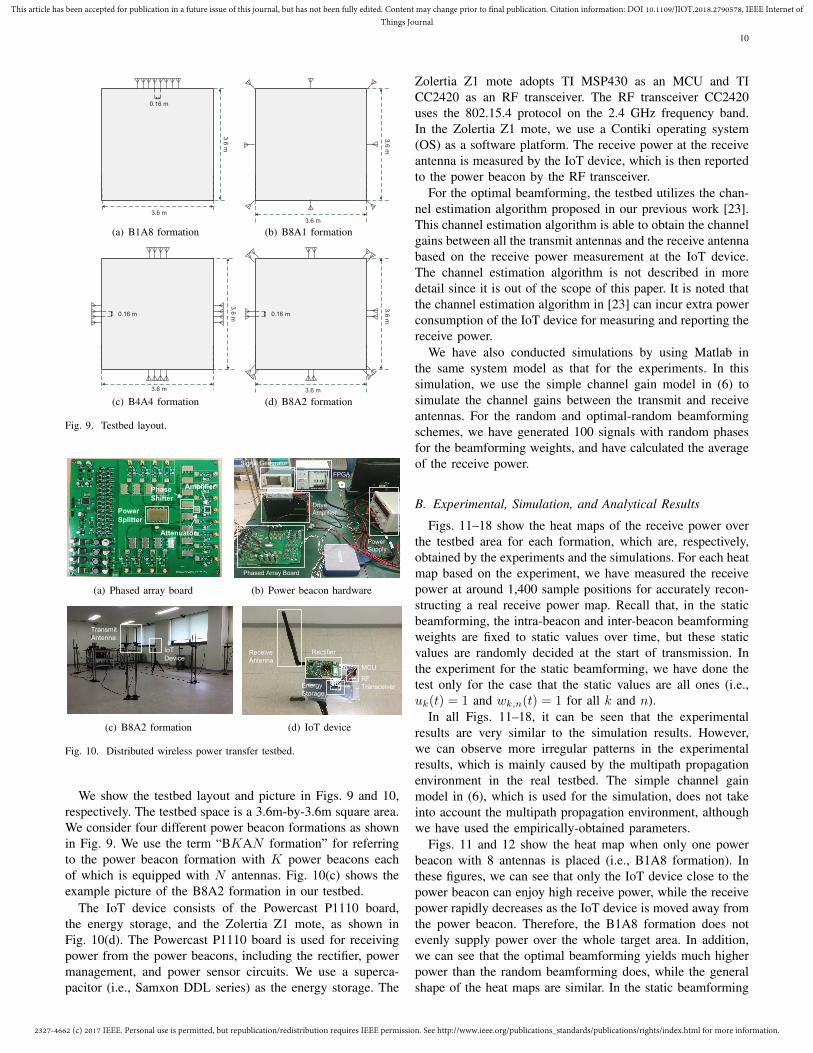
We show the testbed layout and picture in Figs. 9 and 10,respectively. The testbed space is a 3.6m-by-3.6m square area.We consider four different power beacon formations as shownin Fig. 9. We use the term “BKAN formation” for referringto the power beacon formation with K power beacons eachof which is equipped with N antennas. Fig. 10(c) shows theexample picture of the B8A2 formation in our testbed.

The IoT device consists of the Powercast P1110 board,the energy storage, and the Zolertia Z1 mote, as shown inFig. 10(d). The Powercast P1110 board is used for receivingpower from the power beacons, including the rectifier, powermanagement, and power sensor circuits. We use a superca-pacitor (i.e., Samxon DDL series) as the energy storage. The

Zolertia Z1 mote adopts TI MSP430 as an MCU and TICC2420 as an RF transceiver. The RF transceiver CC2420uses the 802.15.4 protocol on the 2.4 GHz frequency band.In the Zolertia Z1 mote, we use a Contiki operating system(OS) as a software platform. The receive power at the receiveantenna is measured by the IoT device, which is then reportedto the power beacon by the RF transceiver.

For the optimal beamforming, the testbed utilizes the chan-nel estimation algorithm proposed in our previous work [23].This channel estimation algorithm is able to obtain the channelgains between all the transmit antennas and the receive antennabased on the receive power measurement at the IoT device.The channel estimation algorithm is not described in moredetail since it is out of the scope of this paper. It is noted thatthe channel estimation algorithm in [23] can incur extra powerconsumption of the IoT device for measuring and reporting thereceive power.

We have also conducted simulations by using Matlab inthe same system model as that for the experiments. In thissimulation, we use the simple channel gain model in (6) tosimulate the channel gains between the transmit and receiveantennas. For the random and optimal-random beamformingschemes, we have generated 100 signals with random phasesfor the beamforming weights, and have calculated the averageof the receive power.

B. Experimental, Simulation, and Analytical Results

Figs. 11–18 show the heat maps of the receive power overthe testbed area for each formation, which are, respectively,obtained by the experiments and the simulations. For each heatmap based on the experiment, we have measured the receivepower at around 1,400 sample positions for accurately recon-structing a real receive power map. Recall that, in the staticbeamforming, the intra-beacon and inter-beacon beamformingweights are fixed to static values over time, but these staticvalues are randomly decided at the start of transmission. Inthe experiment for the static beamforming, we have done thetest only for the case that the static values are all ones (i.e.,uk(t) = 1 and wk,n(t) = 1 for all k and n).

In all Figs. 11–18, it can be seen that the experimentalresults are very similar to the simulation results. However,we can observe more irregular patterns in the experimentalresults, which is mainly caused by the multipath propagationenvironment in the real testbed. The simple channel gainmodel in (6), which is used for the simulation, does not takeinto account the multipath propagation environment, althoughwe have used the empirically-obtained parameters.

Figs. 11 and 12 show the heat map when only one powerbeacon with 8 antennas is placed (i.e., B1A8 formation). Inthese figures, we can see that only the IoT device close to thepower beacon can enjoy high receive power, while the receivepower rapidly decreases as the IoT device is moved away fromthe power beacon. Therefore, the B1A8 formation does notevenly supply power over the whole target area. In addition,we can see that the optimal beamforming yields much higherpower than the random beamforming does, while the generalshape of the heat maps are similar. In the static beamforming



11

-1.5 -1.2 -0.9 -0.6 -0.3 0.0 0.3 0.6 0.9 1.2 1.5

-1.5

-1.2

-0.9

-0.6

-0.3

0.0

0.3

0.6

0.9

1.2

1.5

Y-p

osi

tio

n (

met

er)

X-position (meter)

-20.00

-16.25

-12.50

-8.750

-5.000

-1.250

2.500

6.250

10.00

Power (dBm)

(a) Optimal

-1.5 -1.2 -0.9 -0.6 -0.3 0.0 0.3 0.6 0.9 1.2 1.5

-1.5

-1.2

-0.9

-0.6

-0.3

0.0

0.3

0.6

0.9

1.2

1.5

Y-p

osi

tio

n (

met

er)

X-position (meter)

-20.00

-16.25

-12.50

-8.750

-5.000

-1.250

2.500

6.250

10.00

Power (dBm)

(b) Random

-1.5 -1.2 -0.9 -0.6 -0.3 0.0 0.3 0.6 0.9 1.2 1.5

-1.5

-1.2

-0.9

-0.6

-0.3

0.0

0.3

0.6

0.9

1.2

1.5

Y-p

osi

tio

n (

met

er)

X-position (meter)

-20.00

-16.25

-12.50

-8.750

-5.000

-1.250

2.500

6.250

10.00

Power (dBm)

(c) Static

Fig. 11. Experimental results of receive power heat maps in B1A8 formation.

-1.5 -1.2 -0.9 -0.6 -0.3 0.0 0.3 0.6 0.9 1.2 1.5

-1.5

-1.2

-0.9

-0.6

-0.3

0.0

0.3

0.6

0.9

1.2

1.5

Y-p

osi

tio

n (

met

er)

X-position (meter)

-20.00

-16.25

-12.50

-8.750

-5.000

-1.250

2.500

6.250

10.00

Power (dBm)

(a) Optimal

-1.5 -1.2 -0.9 -0.6 -0.3 0.0 0.3 0.6 0.9 1.2 1.5

-1.5

-1.2

-0.9

-0.6

-0.3

0.0

0.3

0.6

0.9

1.2

1.5

Y-p

osi

tio

n (

met

er)

X-position (meter)

-20.00

-16.25

-12.50

-8.750

-5.000

-1.250

2.500

6.250

10.00

Power (dBm)

(b) Random

-1.5 -1.2 -0.9 -0.6 -0.3 0.0 0.3 0.6 0.9 1.2 1.5

-1.5

-1.2

-0.9

-0.6

-0.3

0.0

0.3

0.6

0.9

1.2

1.5

Y-p

osi

tio

n (

met

er)

X-position (meter)

-20.00

-16.25

-12.50

-8.750

-5.000

-1.250

2.500

6.250

10.00

Power (dBm)

(c) Static

Fig. 12. Simulation results of receive power heat maps in B1A8 formation.

-1.5 -1.2 -0.9 -0.6 -0.3 0.0 0.3 0.6 0.9 1.2 1.5

-1.5

-1.2

-0.9

-0.6

-0.3

0.0

0.3

0.6

0.9

1.2

1.5

Y-p

osi

tio

n (

met

er)

X-position (meter)

-20.00

-16.25

-12.50

-8.750

-5.000

-1.250

2.500

6.250

10.00

Power (dBm)

(a) Optimal

-1.5 -1.2 -0.9 -0.6 -0.3 0.0 0.3 0.6 0.9 1.2 1.5

-1.5

-1.2

-0.9

-0.6

-0.3

0.0

0.3

0.6

0.9

1.2

1.5

Y-p

osi

tio

n (

met

er)

X-position (meter)

-20.00

-16.25

-12.50

-8.750

-5.000

-1.250

2.500

6.250

10.00

Power (dBm)

(b) Random

-1.5 -1.2 -0.9 -0.6 -0.3 0.0 0.3 0.6 0.9 1.2 1.5

-1.5

-1.2

-0.9

-0.6

-0.3

0.0

0.3

0.6

0.9

1.2

1.5

Y-p

osi

tio

n (

met

er)

X-position (meter)

-20.00

-16.25

-12.50

-8.750

-5.000

-1.250

2.500

6.250

10.00

Power (dBm)

(c) Static


-1.5 -1.2 -0.9 -0.6 -0.3 0.0 0.3 0.6 0.9 1.2 1.5

-1.5

-1.2

-0.9

-0.6

-0.3

0.0

0.3

0.6

0.9

1.2

1.5

Y-p

osi

tio

n (

met

er)

X-position (meter)

-20.00

-16.25

-12.50

-8.750

-5.000

-1.250

2.500

6.250

10.00

Power (dBm)

(a) Optimal

-1.5 -1.2 -0.9 -0.6 -0.3 0.0 0.3 0.6 0.9 1.2 1.5

-1.5

-1.2

-0.9

-0.6

-0.3

0.0

0.3

0.6

0.9

1.2

1.5

Y-p

osi

tio

n (

met

er)

X-position (meter)

-20.00

-16.25

-12.50

-8.750

-5.000

-1.250

2.500

6.250

10.00

Power (dBm)

(b) Random

-1.5 -1.2 -0.9 -0.6 -0.3 0.0 0.3 0.6 0.9 1.2 1.5

-1.5

-1.2

-0.9

-0.6

-0.3

0.0

0.3

0.6

0.9

1.2

1.5

Y-p

osi

tio

n (

met

er)

X-position (meter)

-20.00

-16.25

-12.50

-8.750

-5.000

-1.250

2.500

6.250

10.00

Power (dBm)

(c) Static




12

case, we can see that an RF beam is formed in both theexperimental and simulation results, since the same phasesare excited in all transmit antennas. The IoT device outside ofthe RF beam can only receive very small power since the RFsignals from multiple antennas are destructively combined insuch places.

In Figs. 13 and 14, the heat map of the receive power inthe case of the B8A1 formation is shown. In contrast to theB1A8 formation, the whole testbed area is surrounded by 8antennas in the B8A1 formation. As a result, we can observethat the receive power is evenly distributed over the whole areain the optimal and random beamforming cases. Therefore, itis expected that the B8A1 formation is more advantageousthan the B1A8 formation in terms of the coverage probabilitywhen the receive power threshold is moderately set. In thestatic beamforming case, we can observe that the heat mapis riddled with “holes” with very low receive power, wherethe RF signals are destructively combined. This means that alot of blind spots of no power supply can arise if the staticbeamforming is used.

Figs. 15–18 show the heat map in the cases of the B4A4 andB8A2 formations, respectively. In these formations, we alsopresent the optimal-random beamforming case in which theoptimal beamforming is performed within each power beacon,but the phases of different power beacons are randomized dueto the lack of cooperation between power beacons. As ex-pected, the performance of the optimal-random beamformingis somewhere in between those of the optimal and the randombeamforming schemes. With the number of transmit antennastwice higher than that of the B1A8 and B8A1 formations, theoptimal beamforming in the B4A4 and B8A2 formations isable to cover the whole testbed area with quite high receivepower.

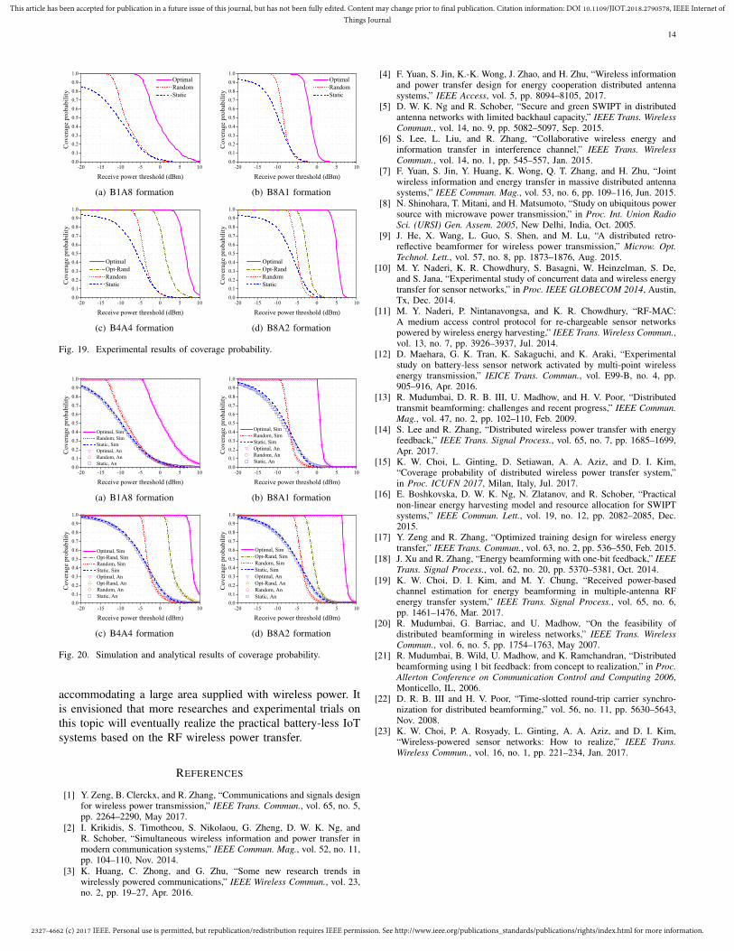
In Figs. 19 and 20, we show the coverage probability, whichis defined as the probability of the receive power no lessthan a given receive power threshold. These graphs show thecoverage probability for the given receive power thresholdon the x-axis. The coverage probability from the experimentsare shown Figs. 19, while that from the simulation and theanalysis are shown in Fig. 20. In Fig. 20, the simulation andthe analytical results are, respectively, denoted by “Sim” and“An”. The coverage probabilities from the experiments and thesimulations are obtained based on their respective heat mapsof the receive power. On the other hand, the analysis results ofthe coverage probability are derived from the simple equationsintroduced in Section IV.

In Figs. 19 and 20, we can see that the experimental resultsvery well matches with the simulation and analytical resultsfor all formations and beamforming schemes, in spite of thesimplified channel model for the simulation and the analysis.This means that the simple analytic equations in Section IVcan be used for predicting the coverage probability beforeactually developing and installing the distributed wirelesspower transfer systems with various beamforming schemes.

In these figures, we can see that the receive power dis-tribution of the B1A8 formation is more dispersed than thatof the B8A1 formation since the IoT device close to theonly power beacon in the B1A8 formation can receive high

power while that far from the power beacon receives verysmall power. This leads to the potential benefit of using manyspatially distributed power beacons with a smaller number ofantennas over using one power beacon with many antennas,when the receive power threshold is moderately low. Forexample, in the experimental results in Figs. 19(a) and 19(b),if the optimal beamforming is used and the receive powerthreshold is -3 dBm, the coverage probability of the B8A1formation is around 0.85 while that of the B1A8 formationis around 0.75. In the analytical results in Figs. 20(a) and20(b), this performance gap is shown to be much bigger, thatis, if the receive power threshold is 0 dBm, the coverageprobability of the B8A1 formation is close to 1 while thatof the B1A8 formation is around 0.55. If the inter-beaconbeamforming is not available, this advantage of using spatiallydistributed power beacons may not be attained because ofthe large performance gap between the optimal and randombeamforming schemes.

These figures also show the disadvantage of the staticbeamforming. We can see that, if the static beamforming isused, there are many places where the receive power is verylow due to the destructive combination of the RF signals.Therefore, if the optimal beamforming is not available, itwould be better to randomize the phases of the transmit signalsto average out the receive power.

VI. CONCLUSION

In this paper, we have suggested the potential architec-tures of the distributed wireless power transfer system, andhave investigated the phase and frequency synchronizationproblems that might arise in the distributed architecture. Wehave analyzed the receive power according to various intra-beacon and inter-beacon beamforming schemes. We have alsoconducted extensive experiments on a real testbed to seehow the receive power is distributed within a confined area.We have shown that the experiment results very well agreewith the analytical results, which proves the usefulness of theproposed analytic formula in designing the distributed wirelesspower transfer system. The experimental results show thatusing spatially distributed power beacons with a single antennacan be advantageous over using a single power beacon withmany antennas in terms of the coverage probability. However,this advantage is achieved only when the optimal inter-beaconbeamforming can be realized in the distributed antenna system.The optimal inter-beacon beamforming requires the frequencysynchronization in the oscillators as well as the beamformingcoordinations between different power beacons. Therefore,further research on the optimal inter-beacon beamformingschemes should be done to realize the full potential of thedistributed wireless power transfer system.

For expediting the adoption of the RF wireless power trans-fer in the practical IoT systems, it is very crucial to extend thecoverage area of the wireless power transfer with sufficientlyhigh power transfer efficiency so that the wireless powertransfer can be applied to the wide range of IoT applications.The proposed distributed wireless power transfer along withthe beamforming is a strong enabling candidate technology for



13

-1.5 -1.2 -0.9 -0.6 -0.3 0.0 0.3 0.6 0.9 1.2 1.5

-1.5

-1.2

-0.9

-0.6

-0.3

0.0

0.3

0.6

0.9

1.2

1.5

Y-p

osi

tio

n (

met

er)

X-position (meter)

-20.00

-16.25

-12.50

-8.750

-5.000

-1.250

2.500

6.250

10.00

Power (dBm)

(a) Optimal

-1.5 -1.2 -0.9 -0.6 -0.3 0.0 0.3 0.6 0.9 1.2 1.5

-1.5

-1.2

-0.9

-0.6

-0.3

0.0

0.3

0.6

0.9

1.2

1.5

Y-p

osi

tio

n (

met

er)

X-position (meter)

-20.00

-16.25

-12.50

-8.750

-5.000

-1.250

2.500

6.250

10.00

Power (dBm)

(b) Optimal-random

-1.5 -1.2 -0.9 -0.6 -0.3 0.0 0.3 0.6 0.9 1.2 1.5

-1.5

-1.2

-0.9

-0.6

-0.3

0.0

0.3

0.6

0.9

1.2

1.5

Y-p

osi

tio

n (

met

er)

X-position (meter)

-20.00

-16.25

-12.50

-8.750

-5.000

-1.250

2.500

6.250

10.00

Power (dBm)

(c) Random

-1.5 -1.2 -0.9 -0.6 -0.3 0.0 0.3 0.6 0.9 1.2 1.5

-1.5

-1.2

-0.9

-0.6

-0.3

0.0

0.3

0.6

0.9

1.2

1.5

Y-p

osi

tio

n (

met

er)

X-position (meter)

-20.00

-16.25

-12.50

-8.750

-5.000

-1.250

2.500

6.250

10.00

Power (dBm)

(d) Static


-1.5 -1.2 -0.9 -0.6 -0.3 0.0 0.3 0.6 0.9 1.2 1.5

-1.5

-1.2

-0.9

-0.6

-0.3

0.0

0.3

0.6

0.9

1.2

1.5

Y-p

osi

tio

n (

met

er)

X-position (meter)

-20.00

-16.25

-12.50

-8.750

-5.000

-1.250

2.500

6.250

10.00

Power (dBm)

(a) Optimal

-1.5 -1.2 -0.9 -0.6 -0.3 0.0 0.3 0.6 0.9 1.2 1.5

-1.5

-1.2

-0.9

-0.6

-0.3

0.0

0.3

0.6

0.9

1.2

1.5

Y-p

osi

tio

n (

met

er)

X-position (meter)

-20.00

-16.25

-12.50

-8.750

-5.000

-1.250

2.500

6.250

10.00

Power (dBm)

(b) Optimal-random

-1.5 -1.2 -0.9 -0.6 -0.3 0.0 0.3 0.6 0.9 1.2 1.5

-1.5

-1.2

-0.9

-0.6

-0.3

0.0

0.3

0.6

0.9

1.2

1.5

Y-p

osi

tio

n (

met

er)

X-position (meter)

-20.00

-16.25

-12.50

-8.750

-5.000

-1.250

2.500

6.250

10.00

Power (dBm)

(c) Random

-1.5 -1.2 -0.9 -0.6 -0.3 0.0 0.3 0.6 0.9 1.2 1.5

-1.5

-1.2

-0.9

-0.6

-0.3

0.0

0.3

0.6

0.9

1.2

1.5

Y-p

osi

tio

n (

met

er)

X-position (meter)

-20.00

-16.25

-12.50

-8.750

-5.000

-1.250

2.500

6.250

10.00

Power (dBm)

(d) Static


-1.5 -1.2 -0.9 -0.6 -0.3 0.0 0.3 0.6 0.9 1.2 1.5

-1.5

-1.2

-0.9

-0.6

-0.3

0.0

0.3

0.6

0.9

1.2

1.5

Y-p

osi

tio

n (

met

er)

X-position (meter)

-20.00

-16.25

-12.50

-8.750

-5.000

-1.250

2.500

6.250

10.00

Power (dBm)

(a) Optimal

-1.5 -1.2 -0.9 -0.6 -0.3 0.0 0.3 0.6 0.9 1.2 1.5

-1.5

-1.2

-0.9

-0.6

-0.3

0.0

0.3

0.6

0.9

1.2

1.5

Y-p

osi

tio

n (

met

er)

X-position (meter)

-20.00

-16.25

-12.50

-8.750

-5.000

-1.250

2.500

6.250

10.00

Power (dBm)

(b) Optimal-random

-1.5 -1.2 -0.9 -0.6 -0.3 0.0 0.3 0.6 0.9 1.2 1.5

-1.5

-1.2

-0.9

-0.6

-0.3

0.0

0.3

0.6

0.9

1.2

1.5

Y-p

osi

tio

n (

met

er)

X-position (meter)

-20.00

-16.25

-12.50

-8.750

-5.000

-1.250

2.500

6.250

10.00

Power (dBm)

(c) Random

-1.5 -1.2 -0.9 -0.6 -0.3 0.0 0.3 0.6 0.9 1.2 1.5

-1.5

-1.2

-0.9

-0.6

-0.3

0.0

0.3

0.6

0.9

1.2

1.5

Y-p

osi

tio

n (

met

er)

X-position (meter)

-20.00

-16.25

-12.50

-8.750

-5.000

-1.250

2.500

6.250

10.00

Power (dBm)

(d) Static


-1.5 -1.2 -0.9 -0.6 -0.3 0.0 0.3 0.6 0.9 1.2 1.5

-1.5

-1.2

-0.9

-0.6

-0.3

0.0

0.3

0.6

0.9

1.2

1.5

Y-p

osi

tio

n (

met

er)

X-position (meter)

-20.00

-16.25

-12.50

-8.750

-5.000

-1.250

2.500

6.250

10.00

Power (dBm)

(a) Optimal

-1.5 -1.2 -0.9 -0.6 -0.3 0.0 0.3 0.6 0.9 1.2 1.5

-1.5

-1.2

-0.9

-0.6

-0.3

0.0

0.3

0.6

0.9

1.2

1.5

Y-p

osi

tio

n (

met

er)

X-position (meter)

-20.00

-16.25

-12.50

-8.750

-5.000

-1.250

2.500

6.250

10.00

Power (dBm)

(b) Optimal-random

-1.5 -1.2 -0.9 -0.6 -0.3 0.0 0.3 0.6 0.9 1.2 1.5

-1.5

-1.2

-0.9

-0.6

-0.3

0.0

0.3

0.6

0.9

1.2

1.5

Y-p

osi

tio

n (

met

er)

X-position (meter)

-20.00

-16.25

-12.50

-8.750

-5.000

-1.250

2.500

6.250

10.00

Power (dBm)

(c) Random

-1.5 -1.2 -0.9 -0.6 -0.3 0.0 0.3 0.6 0.9 1.2 1.5

-1.5

-1.2

-0.9

-0.6

-0.3

0.0

0.3

0.6

0.9

1.2

1.5

Y-p

osi

tio

n (

met

er)

X-position (meter)

-20.00

-16.25

-12.50

-8.750

-5.000

-1.250

2.500

6.250

10.00

Power (dBm)

(d) Static




14

-20 -15 -10 -5 0 5 100.0

0.1

0.2

0.3

0.4

0.5

0.6

0.7

0.8

0.9

1.0

C

ov

era

ge p

rob

ab

ilit

y

Receive power threshold (dBm)

Optimal

Random

Static

(a) B1A8 formation

-20 -15 -10 -5 0 5 100.0

0.1

0.2

0.3

0.4

0.5

0.6

0.7

0.8

0.9

1.0

Co

vera

ge p

rob

ab

ilit

y


Optimal

Random

Static

(b) B8A1 formation

-20 -15 -10 -5 0 5 100.0

0.1

0.2

0.3

0.4

0.5

0.6

0.7

0.8

0.9

1.0

Co

vera

ge p

rob

ab

ilit

y


Optimal

Opt-Rand

Random

Static

(c) B4A4 formation

-20 -15 -10 -5 0 5 100.0

0.1

0.2

0.3

0.4

0.5

0.6

0.7

0.8

0.9

1.0

Co

vera

ge p

rob

ab

ilit

y


Optimal

Opt-Rand

Random

Static

(d) B8A2 formation

Fig. 19. Experimental results of coverage probability.

-20 -15 -10 -5 0 5 100.0

0.1

0.2

0.3

0.4

0.5

0.6

0.7

0.8

0.9

1.0

Co

vera

ge p

rob

ab

ilit

y


Optimal, Sim

Random, Sim

Static, Sim

Optimal, An

Random, An

Static, An

(a) B1A8 formation

-20 -15 -10 -5 0 5 100.0

0.1

0.2

0.3

0.4

0.5

0.6

0.7

0.8

0.9

1.0

Co

vera

ge p

rob

ab

ilit

y


Optimal, Sim

Random, Sim

Static, Sim

Optimal, An

Random, An

Static, An

(b) B8A1 formation

-20 -15 -10 -5 0 5 100.0

0.1

0.2

0.3

0.4

0.5

0.6

0.7

0.8

0.9

1.0

Co

vera

ge p

rob

ab

ilit

y


Optimal, Sim

Opt-Rand, Sim

Random, Sim

Static, Sim

Optimal, An

Opt-Rand, An

Random, An

Static, An

(c) B4A4 formation

-20 -15 -10 -5 0 5 100.0

0.1

0.2

0.3

0.4

0.5

0.6

0.7

0.8

0.9

1.0

Co

vera

ge p

rob

ab

ilit

y


Optimal, Sim

Opt-Rand, Sim

Random, Sim

Static, Sim

Optimal, An

Opt-Rand, An

Random, An

Static, An

(d) B8A2 formation

Fig. 20. Simulation and analytical results of coverage probability.

accommodating a large area supplied with wireless power. Itis envisioned that more researches and experimental trials onthis topic will eventually realize the practical battery-less IoTsystems based on the RF wireless power transfer.

REFERENCES

[1] Y. Zeng, B. Clerckx, and R. Zhang, “Communications and signals designfor wireless power transmission,” IEEE Trans. Commun., vol. 65, no. 5,pp. 2264–2290, May 2017.

[2] I. Krikidis, S. Timotheou, S. Nikolaou, G. Zheng, D. W. K. Ng, andR. Schober, “Simultaneous wireless information and power transfer inmodern communication systems,” IEEE Commun. Mag., vol. 52, no. 11,pp. 104–110, Nov. 2014.

[3] K. Huang, C. Zhong, and G. Zhu, “Some new research trends inwirelessly powered communications,” IEEE Wireless Commun., vol. 23,no. 2, pp. 19–27, Apr. 2016.

[4] F. Yuan, S. Jin, K.-K. Wong, J. Zhao, and H. Zhu, “Wireless informationand power transfer design for energy cooperation distributed antennasystems,” IEEE Access, vol. 5, pp. 8094–8105, 2017.

[5] D. W. K. Ng and R. Schober, “Secure and green SWIPT in distributedantenna networks with limited backhaul capacity,” IEEE Trans. WirelessCommun., vol. 14, no. 9, pp. 5082–5097, Sep. 2015.

[6] S. Lee, L. Liu, and R. Zhang, “Collaborative wireless energy andinformation transfer in interference channel,” IEEE Trans. WirelessCommun., vol. 14, no. 1, pp. 545–557, Jan. 2015.

[7] F. Yuan, S. Jin, Y. Huang, K. Wong, Q. T. Zhang, and H. Zhu, “Jointwireless information and energy transfer in massive distributed antennasystems,” IEEE Commun. Mag., vol. 53, no. 6, pp. 109–116, Jun. 2015.

[8] N. Shinohara, T. Mitani, and H. Matsumoto, “Study on ubiquitous powersource with microwave power transmission,” in Proc. Int. Union RadioSci. (URSI) Gen. Assem. 2005, New Delhi, India, Oct. 2005.

[9] J. He, X. Wang, L. Guo, S. Shen, and M. Lu, “A distributed retro-reflective beamformer for wireless power transmission,” Microw. Opt.Technol. Lett., vol. 57, no. 8, pp. 1873–1876, Aug. 2015.

[10] M. Y. Naderi, K. R. Chowdhury, S. Basagni, W. Heinzelman, S. De,and S. Jana, “Experimental study of concurrent data and wireless energytransfer for sensor networks,” in Proc. IEEE GLOBECOM 2014, Austin,Tx, Dec. 2014.

[11] M. Y. Naderi, P. Nintanavongsa, and K. R. Chowdhury, “RF-MAC:A medium access control protocol for re-chargeable sensor networkspowered by wireless energy harvesting,” IEEE Trans. Wireless Commun.,vol. 13, no. 7, pp. 3926–3937, Jul. 2014.

[12] D. Maehara, G. K. Tran, K. Sakaguchi, and K. Araki, “Experimentalstudy on battery-less sensor network activated by multi-point wirelessenergy transmission,” IEICE Trans. Commun., vol. E99-B, no. 4, pp.905–916, Apr. 2016.

[13] R. Mudumbai, D. R. B. III, U. Madhow, and H. V. Poor, “Distributedtransmit beamforming: challenges and recent progress,” IEEE Commun.Mag., vol. 47, no. 2, pp. 102–110, Feb. 2009.

[14] S. Lee and R. Zhang, “Distributed wireless power transfer with energyfeedback,” IEEE Trans. Signal Process., vol. 65, no. 7, pp. 1685–1699,Apr. 2017.

[15] K. W. Choi, L. Ginting, D. Setiawan, A. A. Aziz, and D. I. Kim,“Coverage probability of distributed wireless power transfer system,”in Proc. ICUFN 2017, Milan, Italy, Jul. 2017.

[16] E. Boshkovska, D. W. K. Ng, N. Zlatanov, and R. Schober, “Practicalnon-linear energy harvesting model and resource allocation for SWIPTsystems,” IEEE Commun. Lett., vol. 19, no. 12, pp. 2082–2085, Dec.2015.

[17] Y. Zeng and R. Zhang, “Optimized training design for wireless energytransfer,” IEEE Trans. Commun., vol. 63, no. 2, pp. 536–550, Feb. 2015.

[18] J. Xu and R. Zhang, “Energy beamforming with one-bit feedback,” IEEETrans. Signal Process., vol. 62, no. 20, pp. 5370–5381, Oct. 2014.

[19] K. W. Choi, D. I. Kim, and M. Y. Chung, “Received power-basedchannel estimation for energy beamforming in multiple-antenna RFenergy transfer system,” IEEE Trans. Signal Process., vol. 65, no. 6,pp. 1461–1476, Mar. 2017.

[20] R. Mudumbai, G. Barriac, and U. Madhow, “On the feasibility ofdistributed beamforming in wireless networks,” IEEE Trans. WirelessCommun., vol. 6, no. 5, pp. 1754–1763, May 2007.

[21] R. Mudumbai, B. Wild, U. Madhow, and K. Ramchandran, “Distributedbeamforming using 1 bit feedback: from concept to realization,” in Proc.Allerton Conference on Communication Control and Computing 2006,Monticello, IL, 2006.

[22] D. R. B. III and H. V. Poor, “Time-slotted round-trip carrier synchro-nization for distributed beamforming,” vol. 56, no. 11, pp. 5630–5643,Nov. 2008.

[23] K. W. Choi, P. A. Rosyady, L. Ginting, A. A. Aziz, and D. I. Kim,“Wireless-powered sensor networks: How to realize,” IEEE Trans.Wireless Commun., vol. 16, no. 1, pp. 221–234, Jan. 2017.

distributed wireless power transfer system for internet-of

Documents