distributed internet security and
TRANSCRIPT

Distributed Internet Security andMeasurement
by
Josh Karlin
B.A., Computer Science and Mathematics, Hendrix College, 2002
DISSERTATION
Submitted in Partial Fulfillment of the
Requirements for the Degree of
Doctor of Philosophy
Computer Science
The University of New Mexico
Albuquerque, New Mexico
May, 2009

c©2009, Josh Karlin
iii

Dedication
To my lovely, smelly dog.
iv

Acknowledgments
I would like to thank my advisor, Stephanie Forrest, for her insight, confidence, anddedicated mentorship. I would also like to thank Jennifer Rexford, Barney Maccabe,Patrick Bridges, Darko Stefanovic, and Jed Crandall for taking so much of their timeto work with me.
I am grateful to my family for their constant encouragement and motivation. Iwould especially like to thank my wife, Shelly, for her understanding and supportwhen deadlines drew near.
Finally, I would like to thank the members of the Adaptive Computation Labo-ratory for their help, creative discussions, and their friendship.
v

Distributed Internet Security andMeasurement
by
Josh Karlin
ABSTRACT OF DISSERTATION
Submitted in Partial Fulfillment of the
Requirements for the Degree of
Doctor of Philosophy
Computer Science
The University of New Mexico
Albuquerque, New Mexico
May, 2009

Distributed Internet Security andMeasurement
by
Josh Karlin
B.A., Computer Science and Mathematics, Hendrix College, 2002
Ph.D., Computer Science, University of New Mexico, 2009
Abstract
The Internet has developed into an important economic, military, academic, and
social resource. It is a complex network, comprised of tens of thousands of indepen-
dently operated networks, called Autonomous Systems (ASes). A significant strength
of the Internet’s design, one which enabled its rapid growth in terms of users and
bandwidth, is that its underlying protocols (such as IP, TCP, and BGP) are dis-
tributed. Users and networks alike can attach and detach from the Internet at will,
without causing major disruptions to global Internet connectivity.
This dissertation shows that the Internet’s distributed, and often redundant struc-
ture, can be exploited to increase the security of its protocols, particularly BGP
(the Internet’s interdomain routing protocol). It introduces Pretty Good BGP, an
anomaly detection protocol coupled with an automated response that can protect
individual networks from BGP attacks. It also presents statistical measurements of
the Internet’s structure and uses them to create a model of Internet growth. This
vii

work could be used, for instance, to test upcoming routing protocols on ensemble of
large, Internet-like graphs. Finally, this dissertation shows that while the Internet
is designed to be agnostic to political influence, it is actually quite centralized at
the country level. With the recent rise in country-level Internet policies, such as
nation-wide censorship and warrantless wiretaps, this centralized control could have
significant impact on international reachability.
viii

Contents
List of Figures xiii
List of Tables xvi
Glossary xvii
1 Introduction 1
1.1 Distributed Routing Security: Pretty Good BGP . . . . . . . . . . . 4
1.2 Measuring and Modeling the AS Level Graph . . . . . . . . . . . . . 5
1.3 Nation-State Routing . . . . . . . . . . . . . . . . . . . . . . . . . . . 6
1.4 Outline of Dissertation . . . . . . . . . . . . . . . . . . . . . . . . . . 7
2 Background and Related Work 9
2.1 BGP and the AS-Level Topology . . . . . . . . . . . . . . . . . . . . 9
2.2 BGP’s History . . . . . . . . . . . . . . . . . . . . . . . . . . . . . . . 13
2.3 BGP’s Vulnerabilities . . . . . . . . . . . . . . . . . . . . . . . . . . . 14
ix
Contents
2.3.1 Origin AS Attacks . . . . . . . . . . . . . . . . . . . . . . . . 14
2.3.2 Invalid Paths . . . . . . . . . . . . . . . . . . . . . . . . . . . 16
2.4 Related Work . . . . . . . . . . . . . . . . . . . . . . . . . . . . . . . 18
2.4.1 BGP Security Proposals . . . . . . . . . . . . . . . . . . . . . 19
2.4.2 Inferring BGP Paths . . . . . . . . . . . . . . . . . . . . . . . 24
2.4.3 Modeling the AS Network . . . . . . . . . . . . . . . . . . . . 27
3 Pretty Good BGP Design and Implementation 29
3.1 Pretty Good BGP (PGBGP) . . . . . . . . . . . . . . . . . . . . . . 30
3.1.1 Anomaly detection . . . . . . . . . . . . . . . . . . . . . . . . 31
3.1.2 Response . . . . . . . . . . . . . . . . . . . . . . . . . . . . . 33
3.1.3 Correctness of PGBGP . . . . . . . . . . . . . . . . . . . . . . 34
3.1.4 Responding to Long-Term Attacks . . . . . . . . . . . . . . . 36
3.2 Comparison to Other BGP Security Approaches . . . . . . . . . . . . 37
3.3 Implementation . . . . . . . . . . . . . . . . . . . . . . . . . . . . . . 39
3.3.1 PGBGP in Quagga . . . . . . . . . . . . . . . . . . . . . . . . 40
3.3.2 The Internet Alert Registry . . . . . . . . . . . . . . . . . . . 42
3.4 Summary . . . . . . . . . . . . . . . . . . . . . . . . . . . . . . . . . 43
4 Pretty Good BGP: Experimental Results 45
4.1 Incremental Adoption . . . . . . . . . . . . . . . . . . . . . . . . . . . 46
x

Contents
4.1.1 Experimental Setup . . . . . . . . . . . . . . . . . . . . . . . . 46
4.1.2 Unprotected Networks . . . . . . . . . . . . . . . . . . . . . . 48
4.1.3 Incremental Adoption . . . . . . . . . . . . . . . . . . . . . . 49
4.1.4 Propagation of Anomalous Routes . . . . . . . . . . . . . . . . 50
4.2 Analysis of PGBGP Anomalies . . . . . . . . . . . . . . . . . . . . . 51
4.2.1 Experimental Setup . . . . . . . . . . . . . . . . . . . . . . . . 52
4.2.2 Most Anomalies Disappear Quickly . . . . . . . . . . . . . . . 53
4.2.3 Number of Anomalies . . . . . . . . . . . . . . . . . . . . . . . 55
4.3 Limitations of PGBGP . . . . . . . . . . . . . . . . . . . . . . . . . . 57
4.4 Summary . . . . . . . . . . . . . . . . . . . . . . . . . . . . . . . . . 59
5 Measuring and Modeling the Autonomous System (AS) Level In-
ternet 61
5.1 Measuring the AS Network’s Topology . . . . . . . . . . . . . . . . . 62
5.1.1 Networks . . . . . . . . . . . . . . . . . . . . . . . . . . . . . 63
5.1.2 Numerical results . . . . . . . . . . . . . . . . . . . . . . . . . 67
5.1.3 From Measurement to Modeling . . . . . . . . . . . . . . . . . 79
5.2 Modeling the AS-Level Internet . . . . . . . . . . . . . . . . . . . . . 79
5.2.1 AS Simulation Model (ASIM) . . . . . . . . . . . . . . . . . . 81
5.2.2 Numerical simulations . . . . . . . . . . . . . . . . . . . . . . 87
5.3 Summary . . . . . . . . . . . . . . . . . . . . . . . . . . . . . . . . . 97
xi

Contents
6 Nation-State Routing 99
6.1 The Appropriate Granularity for Analyzing Country-Level Paths . . . 102
6.2 The Country Path Algorithm . . . . . . . . . . . . . . . . . . . . . . 104
6.2.1 Prefix Pair to AS-path . . . . . . . . . . . . . . . . . . . . . . 105
6.2.2 Mapping Traceroutes to AS and Country Paths . . . . . . . . 108
6.2.3 AS-path to Country-path . . . . . . . . . . . . . . . . . . . . 110
6.3 Reachability Metrics . . . . . . . . . . . . . . . . . . . . . . . . . . . 114
6.3.1 Background on Betweenness Centrality . . . . . . . . . . . . . 115
6.3.2 Country Centrality . . . . . . . . . . . . . . . . . . . . . . . . 116
6.3.3 Strong Country Centrality . . . . . . . . . . . . . . . . . . . . 117
6.4 Country Centrality Results . . . . . . . . . . . . . . . . . . . . . . . . 118
6.4.1 Analysis on Directly Observed Paths . . . . . . . . . . . . . . 119
6.4.2 Validation of Inference of Country Paths . . . . . . . . . . . . 121
6.4.3 Analysis on More Complete Country Paths . . . . . . . . . . . 122
6.5 Summary . . . . . . . . . . . . . . . . . . . . . . . . . . . . . . . . . 125
7 Future Work and Conclusion 128
7.1 Future Work . . . . . . . . . . . . . . . . . . . . . . . . . . . . . . . . 128
7.2 Concluding Remarks . . . . . . . . . . . . . . . . . . . . . . . . . . . 131
References 132
xii

List of Figures
2.1 Example BGP route propagation. . . . . . . . . . . . . . . . . . . . 10
2.2 Examples of invalid paths. . . . . . . . . . . . . . . . . . . . . . . . 16
2.3 Examples of shapes that cannot be seen in valid paths. . . . . . . . 17
3.1 Example policy violations. . . . . . . . . . . . . . . . . . . . . . . . 30
3.2 Example policy violations. . . . . . . . . . . . . . . . . . . . . . . . 30
3.3 Example anomalies. . . . . . . . . . . . . . . . . . . . . . . . . . . . 31
3.4 The PGBGP update algorithm. . . . . . . . . . . . . . . . . . . . . 40
3.5 PGBGP Commands . . . . . . . . . . . . . . . . . . . . . . . . . . . 40
3.6 Structures used to store PGBGP’s normal database. . . . . . . . . . 41
4.1 Effectiveness of synthetic BGP attacks without any security protection. 48
4.2 Effectiveness of synthetic BGP attacks with PGBGP. . . . . . . . . 51
4.3 Duration of anomalous events. . . . . . . . . . . . . . . . . . . . . . 53
4.4 The number of prefix hijacks observed over four months. . . . . . . . 54
4.5 The number of sub-prefix hijacks observed over four months. . . . . 54
xiii

List of Figures
4.6 The number of edge anomalies observed over four months. . . . . . . 55
4.7 Effectiveness of PGBGP in a partial deployment. . . . . . . . . . . . 60
5.1 Normalized histograms of vertices with a specific average distance d
to the rest of the vertices. . . . . . . . . . . . . . . . . . . . . . . . . 67
5.2 Degree k as a function of the average distance d. . . . . . . . . . . . 70
5.3 Neighbor degree K as a function of the average distance d. . . . . . 72
5.4 Deletion impact of as a function of the average distance d. . . . . . . 74
5.5 Clustering coefficient C as a function of the average distance d. . . . 76
5.6 Distance balance b as a function of the average distance d. . . . . . . 78
5.7 Illustration of the network growth algorithm. . . . . . . . . . . . . . 82
5.8 Illustration of traffic simulation. . . . . . . . . . . . . . . . . . . . . 85
5.9 Time evolution of an example model run. . . . . . . . . . . . . . . . 89
5.10 The degree distribution of a real AS graph vs generated. . . . . . . . 91
5.11 Radial statistics for real and model networks. . . . . . . . . . . . . . 93
5.12 Traffic patterns of the model. . . . . . . . . . . . . . . . . . . . . . . 94
5.13 Spatial expansion of a single agent. . . . . . . . . . . . . . . . . . . 96
6.1 Example AS topology with AS paths. . . . . . . . . . . . . . . . . . 103
6.2 Traceroutes, AS-paths, and country paths. . . . . . . . . . . . . . . 104
6.3 Pseudo-code of Qiu’s inference algorithm. . . . . . . . . . . . . . . . 105
6.4 Pseudo-code of Qiu’s path comparison heuristic . . . . . . . . . . . . 106
xiv

List of Figures
6.5 Example annotated traceroute . . . . . . . . . . . . . . . . . . . . . 112
6.6 Pseudo-code of AS-path to country-path prediction . . . . . . . . . . 112
6.7 Betweenness Centrality. . . . . . . . . . . . . . . . . . . . . . . . . . 114
6.8 Actual vs predicted Country Centrality. . . . . . . . . . . . . . . . . 122
6.9 Country Centrality on more complete, inferred country-paths. . . . . 123
6.10 Strong Country Centrality (Zoomed). . . . . . . . . . . . . . . . . . 125
xv

List of Tables
2.1 Standard route export rules. . . . . . . . . . . . . . . . . . . . . . . 10
2.2 Invalid path exploits. . . . . . . . . . . . . . . . . . . . . . . . . . . 16
3.1 Comparison of BGP security protocols when ubiquitously deployed. 37
3.2 Comparison of BGP security protocols when partially deployed. . . . 37
4.1 The sum of the absolute difference of the mean between PGBGP’s
effectiveness and the black box filter’s for the plots of Figure 4.7 . . 49
5.1 Default parameters values for simulation experiments. . . . . . . . . 88
6.1 Country Centrality (CC) computed directly from traceroute (TR)
and BGP paths. Numbers in parenthesis represent the country’s
position in the TR column. . . . . . . . . . . . . . . . . . . . . . . . 120
6.2 Country Centrality (CC) and Strong Country Centrality (SCC) com-
puted using inferred country paths . . . . . . . . . . . . . . . . . . . 124
6.3 Country Centrality and Strong Country Centrality values of countries
with pervasive censorship. . . . . . . . . . . . . . . . . . . . . . . . . 126
xvi

Glossary
AS Autonomous System. A (typically multi-homed) network that has
been assigned IP address space and has its own intradomain rout-
ing policies. ISP, university, and corporate networks are often au-
tonomous systems.
BGP Border Gateway Protocol. BGP is a path-vector routing protocol
that finds AS-paths to destination prefixes. It is the de-facto inter-
domain routing protocol.
IP prefix A contiguous block of IP addresses. An example of a prefix is
192.168.1.0/24. The “/24” divides the network portion of the prefix
from the host portion. IPv4 has 32 bit addresses, and therefore the
first 24 bits (192.168.1) name the network, and 256 addresses remain
for the hosts.
IRR Internet Routing Registry. A database of AS number assignment,
IP prefix assignment, and routing policies between ASes.
RIR Regional Internet Registry. RIR’s assign AS numbers and IP address
space to organizations within their designated region.
xvii

Chapter 1
Introduction
Today the Internet is comprised of nearly 31,000 individually operated networks
called Autonomous Systems (ASes). These ASes have administrative control over
their internal networks, including routing protocols, topology, and traffic engineering.
A handful of fundamental protocols (BGP, DNS, IP, UDP, TCP) tie these networks
together into a single interdomain network, the Internet. These protocols are insecure
because they do not authenticate communication end points, routing paths, or even
the resolution of names. They are also considered neutral protocols because they do
not give preference to particular networks, or rely upon trusted authorities. They
thrive in a distributed network in which members may freely come and go and the
majority of administrators (or network operators) are trustworthy.
Recently, these protocols have come under the scrutiny of security researchers
as they have repeatedly been publicly compromised. Specifically, weaknesses in the
BGP interdomain routing protocol, which enables each AS to communicate with all
other ASes, have received public attention. For example, in February of 2008, a
Pakistani ISP used BGP to claim ownership of YouTube Inc.’s IPv4 addresses in
an attempt to prevent Pakistani citizens from viewing YouTube content [1]. The
1

Chapter 1. Introduction
announcement of ownership was accidentally leaked globally and YouTube was un-
reachable for several hours. In August of 2008, at the hacker conference DEFCON,
the conference’s network traffic was rerouted to a middle man where it could be spied
upon, and then forwarded back to the attendees using a BGP hijack [2].
A number of the many proposed security solutions (e.g. DNSSEC, Secure BGP,
Secure Origin BGP) for the fundamental protocols could have been implemented
and deployed by now. However, the previously listed solutions are ineffective when
deployed on a single network. They rely upon a wide deployment to be effective
and therefore networks must wait for the entire community to select and deploy a
security protocol before they can be protected.
The research in this dissertation investigates secure solutions for the fundamen-
tal Internet protocols that have robust deployment paths. Specifically, it describes
a distributed security proposal for BGP, called Pretty Good BGP. It also verifies
PGBGP’s effectiveness through simulation and live experiments. Performing accu-
rate simulations of protocol behavior on the Internet is difficult, as the Internet’s
topology is not well understood [3]. Therefore, this dissertation also explores new
methods for measuring and modeling the Internet’s structure to improve simulation
accuracy.
The Internet measurements were performed both at the AS and country-level.
The AS-level measurements differ from previous research in that they tease apart
the differences in network structure based on location within the Internet’s hierarchy
(from core to periphery), rather than focusing on global Internet properties.
The hierarchical, or radial, analysis can be used to verify that AS models produce
statistically realistic graphs across the hierarchical spectrum. This dissertation finds
that existing AS topology models do not sufficiently capture the Internet’s radial
structure, and introduces a new model, ASIM, that does. ASIM is the first AS
2

Chapter 1. Introduction
model to integrate traffic, economy, and geography. With ASIM, it is possible to
create ensembles of realistic graphs to validate new protocols on today’s networks
and predicted topologies of tomorrow’s.
Internet measurements could also be used to understand how new Internet pro-
tocols and policies might affect international routing. For instance, countries might
wish to avoid routing their traffic through countries that are known to censor or
wiretap international traffic. By studying Internet routing at the country-level, this
dissertation investigates how well distributed the Internet is when politics (such as
nation-wide censorship and wiretapping) are taken into account.
This dissertation addresses the following questions:
1. BGP Security Can the BGP protocol be secured without the use of a PKI?
To what extent? Could such a protocol be backwards compatible and have
strong incentive for early adoption? Regardless of the proposed protocol, is
ubiquitous deployment necessary to minimize the effect of BGP attacks on a
global scale?
2. AS-Level Modeling What is the topology and structure of the Autonomous
System (AS) level Internet? Can the AS graph, be accurately modeled? How
do external factors such as economics and geography affect network growth and
connectivity?
3. Country-Level Routing Measurement How might censorship of Internet traffic
(e.g. Pakistan, Iran, China) and legalized warrantless wiretaps (e.g. U.S.A.,
Sweden) affect countries ability to reach each other? In other words, are some
countries so central to the Internet that other countries must route traffic
through them?
In the remainder of this chapter, I summarize three research projects that address
3

Chapter 1. Introduction
the previous questions, and the contributions that I have made. I then provide an
outline of the remainder of this dissertation.
1.1 Distributed Routing Security: Pretty Good
BGP
The Internet’s interdomain routing protocol, BGP, is vulnerable to a number of
potentially crippling attacks. Several promising cryptography-based solutions have
been proposed, but their adoption has been hindered by the need for community
consensus, cooperation in a Public Key Infrastructure (PKI), and a common security
protocol. Rather than force centralized control in a distributed network, I examine
distributed security methods that are amenable to incremental deployment.
Previous research has shown that anomaly detection can be used to enhance
system security without the need for global cooperation or the need to alter the
underlying system’s protocols [4, 5, 6]. For instance, in [4] operating system calls
are monitored for abnormal behavior which might suggest the presence of malicious
code. In response to suspicious system calls, the anomaly detector throttles the
cycle time given to the anomalous application. Another intrusion detection system,
RIOT [5], monitors IP connections for abnormal behavior and throttles outgoing
connections to hinder the propagation of worms when suspicious behavior is detected.
These protocols couple an effective graduated response to difficult security problems
without altering the underlying protocols or requiring the support of external entities.
Anomaly detection and response mechanisms could help improve security of the
fundamental network protocols as well. For each protocol, anomaly detection could
be used to find activities that exploit its vulnerabilities. For instance, within DNS,
new addresses for typically stable names could be considered suspicious. Upon detec-
4

Chapter 1. Introduction
tion of suspicious activity, an effective security response could be used to prevent it
from causing damage. This could be accomplished in network protocols by delaying
the change in state that the suspicious message would cause. In BGP routers, new
destinations for IP addresses could temporarily be given lower priority over routes
with more stable destinations. During this time the actual owner of the IP addresses
could be informed of the proposed change and allowed to remedy the situation before
the malicious route would have a chance to propagate.
This dissertation describes a distributed anomaly detection and response system
for BGP that provides similar protection as that given by existing methods and has
a more plausible adoption path. Specifically, my dissertation makes the following
contributions: (1) it describes Pretty Good BGP (PGBGP), whose security is com-
parable (but not identical) to Secure Origin BGP; (2) it gives theoretical proofs on
the effectiveness of PGBGP; (3) it reports simulation experiments on a snapshot of
the Internet topology; (4) it quantifies the impact that known exploits could have
on the Internet; (5) it presents a reference implementation of Pretty Good BGP,
developed in the Quagga routing suite; and (6) it determines the minimum number
of ASes that would have to adopt a distributed security solution to provide global
protection against these exploits.
Taken together these results explore the boundary between what can be achieved
with provably secure centralized security mechanisms for BGP and more distributed
approaches that respect the autonomous nature of the Internet.
1.2 Measuring and Modeling the AS Level Graph
The structure of the Internet at the Autonomous System (AS) level has been studied
by Physics, Mathematics and Computer Science communities. In collaboration with
Petter Holme, I extend this work to include features of the core and the periphery.
5
Chapter 1. Introduction
New methods for plotting AS data are also described. They are used to analyze data
sets that have been extended to contain edges missing from earlier collections.
In this work the average distance from one vertex to the rest of the network is
used as the baseline metric for investigating network structure. This is useful for
measuring the characteristics of ASes based upon their distance from the network
core. Common vertex-specific quantities are plotted against this metric to reveal dis-
tinctive characteristics of central and peripheral vertices. Two data sets are analyzed
using these measures as well as two common generative models (Barabasi-Albert [7]
and Inet [8]). There is a clear distinction between the highly connected core and a
sparse periphery. This dissertation also shows that the periphery has a more complex
structure than that predicted by existing estimations and models.
This work also models the Internet’s growth in order to better understand its
present state and to predict its future. To date, Internet models have attempted to
explain one (or two) of the following aspects: network structure, traffic flow, geog-
raphy, and economy. This dissertation’s contributions include: (1) the design and
implementation of an agent-based model that integrates all four network aspects;
(2) to validate the model it compares the model’s output to the measurements de-
scribed earlier; and (3) it discusses how the model can be used to improve topology
measurements and test new Internet routing protocols.
1.3 Nation-State Routing
The treatment of Internet traffic is increasingly affected by national policies that
require the ISPs in a country to adopt common protocols or practices. Examples
include government enforced censorship, wiretapping, and protocol deployment man-
dates for IPv6 and DNSSEC.
6

Chapter 1. Introduction
If an entire nation’s worth of ISPs apply common policies to Internet traffic, the
global implications could be significant. For instance, it is known that a number
of countries censor domestic traffic [9, 10]. How much impact would it have on
international communication if those same countries filtered international traffic?
These kinds of questions are surprisingly difficult to answer, as they require com-
bining information collected at the prefix, Autonomous System, and country level,
and grappling with incomplete knowledge about the AS-level topology and routing
policies.
Chapter 6 develops the first framework for country-level routing analysis, which
allows researchers to answer questions about the influence of each country on the flow
of international traffic. The contributions of this dissertation include: (1) identifying
and addressing the many challenges of inferring country-level paths; (2) developing
network centrality metrics to measure each country’s importance to network reach-
ability; and (3) presenting and validating the results. My results show that some
countries known for their national policies, such as Iran and China, have relatively
little effect on interdomain routing, while three countries (the United States, Great
Britain, and Germany) are central to international reachability, and their policies
thus have huge potential impact.
1.4 Outline of Dissertation
The rest of this dissertation is structured as follows. Chapter 2, presents background
material on the Internet’s topology and history, the BGP protocol and its security
problems, and work related to my research. Following the background chapter, I
describe each of the projects. First, in Chapter 3, I describe the design and imple-
mentation of my security proposal for BGP, Pretty Good BGP (PGBGP). Chapter
4 describes experimental results and analysis of PGBGP. In Chapter 5, I present
7

Chapter 1. Introduction
structural measurements of the AS-level graph. I then describe an agent-based net-
work model called ASIM, and use the structural measurements to verify that the
networks it creates are statistically similar to the real AS-graph. This work was
done in collaboration with Petter Holme. The final component of my dissertation,
which measures the influence of each country over international routing, is presented
in Chapter 6. Finally, I discuss possible future work and conclude in Chapter 7.
8
Chapter 2
Background and Related Work
This chapter provides an overview of how Internet routing works today and describes
the Internet’s AS-level structure. It also reviews prior work related to my disserta-
tion, including existing Border Gateway Protocol (BGP) security proposals, methods
to infer interdomain paths, and existing Internet modeling projects. I first present
an overview of the Internet’s topology and BGP in Section 2.1, and then describe
BGP’s history and its vulnerabilities in Sections 2.2 and 2.3. Finally, I review related
work in Section 2.4.
2.1 BGP and the AS-Level Topology
Internet routing operates at the level of IP address blocks, or prefixes . Regional
Internet Registries (RIRs), such as ARIN, RIPE, and APNIC, allocate IP prefixes
to institutions such as Internet Service Providers. These institutions may, in turn,
subdivide the address blocks and delegate these smaller blocks to other ASs, such
as their customers. Ideally, the RIRs would be notified when changes occur, such as
an AS delegating portions of its address space to other institutions, two institutions
9

Chapter 2. Background and Related Work
Route Learned From Should Export Route toProvider All customersPeer All customersCustomer All neighborsLocal All neighbors
Table 2.1: Standard route export rules. Routes learned from providers are propa-gated to customers, while local routes and those learned from customers are propa-gated to all neighbors.
VerizonAT&TQwest
UNM
Comcast
NM Tech
Timer
Warner
Peer to Peer
Provider to Customer
Sibling to Sibling
67.123.22.0/24
VerizonAT&TQwest
UNM
Comcast
NM Tech
Timer
Warner
Peer to Peer
Provider to Customer
Sibling to Sibling
67.123.22.0/24
VerizonAT&TQwest
UNM
Comcast
NM Tech
Timer
Warner
Peer to Peer
Provider to Customer
Sibling to Sibling
67.123.22.0/24
Figure 2.1: From left to right, Comcast first announces its prefix (67.123.22.0/24)to its providers AT&T and Verizon. Next, AT&T and Verizon each select Comcastas their best (and only) route to the prefix and propagate that to their neighbors.Finally, Qwest select’s Verizon’s route over AT&T’s and propagates the route to itscustomers.
combining their address space after a merger or acquisition, or an institution splitting
its address space after a company break-up. However, the registries are notoriously
out-of-date and incomplete. Ultimately, BGP update messages and the BGP routing
tables themselves are the best indicator of active prefixes and the ASs responsible
for them. BGP tables today contain around 280,000 active prefixes, with prefixes
appearing and disappearing continually.
ASs exchange information about how to reach destination prefixes using the Bor-
der Gateway Protocol (BGP). A router learns how to reach external destination
prefixes via BGP sessions with neighboring ASs. BGP has two kinds of update
10

Chapter 2. Background and Related Work
messages—announcements and withdrawals. Announcements contain information
such as the destination prefix, the announcer’s IP address, and the AS path the route
will take. As the route announcement propagates, each AS adds its own unique AS
number to the path. A withdrawal retracts an earlier announcement. BGP responds
to a withdrawal message by deleting the previously announced route from its routing
table and propagating the withdrawal to its neighbors. BGP routing changes can oc-
cur for many reasons, including equipment failures, software crashes, policy changes,
or malicious attacks. Inferring the cause directly from the BGP update messages is
a fundamentally difficult, if not impossible, problem.
A router with multiple neighbors would likely learn multiple routes for each pre-
fix. The route actually chosen to transmit data is determined by the BGP decision
process . The decision process is a sequence of about a dozen rules that compare one
route to another [11]. Generally, a router prefers routes that conform to the policies
of the local network operator. Next, the router prefers routes with the lowest AS
path length. If multiple equally good routes remain, the router can apply additional
rules, ultimately resolving ties arbitrarily to ensure a single answer. Because the
decision process does not consider traffic load or performance metrics, the selected
route is not necessarily optimal from a performance point of view. An illustration
of BGP propagation is shown in Figure 2.1. In it, Comcast announces the prefix
67.123.22.0/24 to the rest of the network. The “/24” in the prefix shows that all
IP addresses that have the same first 24 bits as 67.123.22.0 are within the prefix’s
range.
In practice, routes are often selected and propagated according to local routing
policies, which are based on the business relationships with neighboring ASs [12, 13].
The most common relationships are customer-provider and peer-peer. In a customer-
provider relationship, the provider ensures that its customer can communicate with
the rest of the Internet by exporting its best route for each prefix, and by exporting
11

Chapter 2. Background and Related Work
the customer’s prefixes to other neighboring ASs. In contrast, the customer does not
propagate routes learned from one provider to another since the customer pays for
the use of such links. In a peer-peer relationship, two ASs connect solely to transfer
traffic between their respective customers. An AS announces only the routes learned
from its customers to its peers. These business relationships drive local preferences,
which in turn influence the decision process. Typically, an AS prefers customer-
learned routes over peer-learned routes, and peer-learned routes over provider-learned
routes.
ASes are often prevented by contractual agreements from forwarding (exporting)
their best routes to all of their neighbors [14]. Routes that are exported in violation of
contractual stipulations are considered policy violations, and are one type of invalid
path. According to Gao [14], an AS should export routes learned from its peers and
providers only to its customers. Routes learned from customers should be exported
to all neighbors. Therefore, an AS should not export a route learned from a provider
or peer to another provider or peer. An AS that does so is considered to be a policy
violator and the resulting AS path is a policy violating path. Table 2.1 lists each of
the export rules in common practice for future reference.
Today, the Internet is comprised of roughly 31,000 Autonomous Systems. Al-
though BGP is flexible enough to allow ASes to inter-connect into any graph struc-
ture, the Internet is hierarchically structured in practice. Networks higher in the
hierarchy transit traffic for the networks under them. A rough estimate from 2007
shows that only 17% of the ASes transit traffic for other ASes 1 and are called transit
networks. The remaining ASes are known as stub networks.
1The number of ASes in the IAR database (discussed in Chapter 3) from June 22nd2007 which did not always occur at the end of an AS path.
12

Chapter 2. Background and Related Work
2.2 BGP’s History
The predecessor to the Border Gateway Protocol, the External Gateway Protocol,
was designed around a central core network, the NSFNET. Each peripheral network
had exactly one path to the core, which formed a tree structure. The tree topology of
the Internet prevented routing loops from forming but it also prevented Autonomous
Systems from connecting to multiple providers (known as multi-homing) and sharing
traffic with nearby networks. Network operators (engineers in charge of the networks)
disregarded these precautions and shared traffic with their neighbors anyway, being
careful not to announce this routing information to other networks in an effort to
avoid loops. Eventually, the network community’s desire for a more flexible routing
policy led to the design of the Border Gateway Protocol.
The Border Gateway Protocol was originally described in RFC 1105 [15], in June,
1989. Unlike EGP, the Exterior Gateway Protocol [16], BGP did not constrain the
network into a strict tree topology. BGP allowed peering Autonomous Systems to
define their relationships flexibly, freeing ASes to multi-home, and negotiate peer-to-
peer relationships. Loops were avoided by transmitting the entire path along with
each route update so that routers could discard routes that included duplicate AS
numbers in the path. BGP’s flexibility also allowed new backbones to be integrated
into the Internet, such as those of the tier 1 ISPs.
In the years since BGP’s introduction, the protocol has undergone three signifi-
cant revisions. First, in 1990, BGP-2 [17] removed the topological constraints that
BGP had originally used and allowed for an arbitrary network topology. BGP-3 [18],
documented in 1991, optimized the exchange of information about previously reach-
able routes. Finally, BGP-4 was introduced in 1994 [19] and revised in 1995 [20]
and 2006 [21]. BGP-4 introduced Classless Inter-Domain Routing (CIDR prefixes).
Before CIDR routing, there were 3 network sizes that allowed for either 28, 216, or 224
13

Chapter 2. Background and Related Work
hosts on the network. CIDR prefixes allow finer control of network size, and waste
fewer addresses.
2.3 BGP’s Vulnerabilities
BGP’s vulnerabilities stem from the fact that the information passed between routers
is not verified. The originating AS of the route may not in fact own the prefix that
the route claims, which is referred to as an origin AS attack. Next, the AS path
itself could be altered, leading to problems with snooping, contract violations, and
spoofed paths. In this section, I describe both types of vulnerabilities.
2.3.1 Origin AS Attacks
There are two main classes of origin AS attacks: prefix hijacks and sub-prefix hijacks.
Because BGP does not validate the origin AS of an update message, a BGP router
can announce any prefix, even those it does not own, which is known as a prefix
hijack. For example, a university could announce that it owns a prefix that actually
belongs to a financial institution, such as a bank. Those ASes that selected the
university’s route would send their data to the wrong destination. The university
could then use the data however it pleased: it could discard it (known as a black
hole); it could read the data and then forward it on to the intended destination [22];
or, it could impersonate the bank’s services to gain passwords (such as a website
login page).
Because an AS can announce any prefix, a network can accidentally or maliciously
announce a subnet of another network’s prefix rather than the whole prefix. This is
known as a sub-prefix hijack. For instance, an AS could announce 12.0.0.0/9 which
is a subnet of AT&T’s 12.0.0.0/8. This is a serious form of attack because routers
14

Chapter 2. Background and Related Work
are designed to forward traffic to the smallest matching subnet. Therefore, routers
would forward all traffic in the range of the sub-prefix to the adversary.
An adversarial AS could also announce a larger network, or supernet, of its vic-
tim’s prefix. Although it has been shown that such hijacks could be used for sending
spam from unused address space [23], it could not be used to divert traffic away from
proper destinations because routers always forward packets to the smallest matching
prefix. In this dissertation I do not consider such attacks.
There are many examples of actual origin AS attacks, including the famous 1997
incident in which a single ISP sub-prefix hijacked the first class-C subnet of ev-
ery announced prefix causing reachability problems for a large number of networks.
On November 30th, 2006 AS 4761 announced at least 4000 prefixes that it did not
own [24], including specific prefixes owned by organizations such as banks, universi-
ties, and large corporations. More recently, on February 24th 2008, AS 17557 (Pak-
istan Telecom) sub-prefix hijacked YouTube’s (http://www.youtube.com/) web-
site [1]. It is generally thought that such attacks are accidental, but they still cause
damage and they occur routinely.
It is worth noting that origin AS attacks could be stopped by using only methods
available to BGP today. BGP implementations often provide programmable filters,
in which operators can program their routers to discard routes that violate certain
conditions. Filters are used by some providers to ensure that their customers an-
nounce routes only for prefixes that they own. If all providers did this, the BGP
network would be safe from origin AS attacks. However, many networks do not filter
effectively, forcing neighboring ASes to infer the validity of routes that originate from
many hops away, an impossible task without an accurate registry. Even careful net-
work operators make mistakes, allowing their customers to announce prefixes they
do not own. For example, AS 2914 (Verio) is well known to run carefully configured
filters for its customers, but it was one of the ASes that allowed its customer (AS
15

Chapter 2. Background and Related Work
Exploit Name Category Procedure
Shortest Spoofed Path Spoofed Edge Erase AS path except for the origin AS before exportShortest Path Policy Violation Replace AS path with shortest path of existing edges to origin ASRedistribution Policy Violation Export route learned from one provider or peer to anotherSpoofed AS Number Invalid AS Number Erase AS path and prepend victim’s AS number
Table 2.2: Invalid path exploits.
C
A
B
DE
Redistribution: (A,B,C,D), (A,E,D)Shortest Path: (A,E,D)Shortest Spoofed Path: (A,D)Spoofed AS Number: (D)
Figure 2.2: Examples of invalid paths. Autonomous System A modifies its AS pathwhen exporting routes to gain access to D’s traffic. The paths listed in the legendare those that A could send to its neighbors for each type of invalid path attack.Arrows point to customers from providers, and undirected edges represent peer-peerrelationships.
4761) to announce Panix’s prefix in the well publicized hijack [25].
2.3.2 Invalid Paths
BGP does not verify the AS path declared in a route update. The path might not
have been traversed by the update, or the path might violate a network’s contractual
policy, or it might not exist. The BGP protocol states that before propagating
an update, each AS must prepend its own AS number to the path and leave the
remainder of it untouched. An adversary could disobey the protocol and edit the
path before propagating it, perhaps to shorten it to attract more traffic.
A consensus does not exist on what aspects of an AS path should be validated. I
define an invalid path as an AS path in which an edge (pair of consecutive ASes in an
AS path) in the path is spoofed (does not actually exist in the physical topology), the
16

Chapter 2. Background and Related Work
Figure 2.3: Examples of shapes that cannot be seen in valid paths. Within thesepaths, a customer or provider propagates a route to another customer or provider.Arrows point at customers and undirected edges denote peering relationships.
path violates a contractual policy, or at least one AS in the path has a spoofed AS
number. This extends the definition introduced in [26] to include policy violations.
The most important examples of known BGP exploits that use invalid paths are
listed below:
1. Shortest spoofed path To avoid prefix hijack detection, an AS could erase the
entire path between itself and the origin AS before propagating a route. This
leaves the apparent (spoofed) edge (Adversary, Origin) at the end of the path.
This is also the shortest path possible between the Adversary and the Origin,
increasing its chances of being selected by upstream ASes.
2. Shortest valid path To perform a hijack but avoid having any spoofed edges
in the path, an adversarial AS might erase the existing path and prepend the
shortest valid path of actual edges between itself and the origin AS.
3. Redistribution attack If a BGP router is not correctly configured, it could ac-
cidentally export routes learned from providers or peers to other providers or
peers, causing a policy violation. This is fairly common as many BGP routers
export all learned routes to all neighbors by default. Accidental policy viola-
17

Chapter 2. Background and Related Work
tions can cause traffic bottlenecks, since customers may not be able to handle
their provider’s traffic loads.
providers might route traffic through their customers, which don’t have enough
bandwidth
The reason that accidental policy violation attacks are harmful is that the
providers (and the provider’s providers) that the customer might export the
route to would be likely to select the customer route for the destination, but
the customer might not be able to cope with such a large amount of traffic.
4. ASN spoof A router could be configured with the AS number of its victim. This
could then be used to originate the victim’s prefix with the legitimate origin
AS. This is a difficult attack to perform because the adversary’s neighbors
would likely discard routes that do not have the correct next-hop AS number.
Therefore, AS A must either convince its neighbors that it is indeed AS V,
convince its neighbors to collude with it, or compromise its neighbor’s routers.
Examples of these attacks are given in Figure 2.2, and a short description of each
type of attack is listed in Table 2.2.
2.4 Related Work
In this section, I review previous research related to my dissertation. First, I discuss
existing BGP security protocols, including those that use cryptographic methods.
Next, I describe known heuristics used to infer the economic relationships between
ASes, and the AS-level paths between each pair of IP prefixes. Finally, I review
existing generative models of Internet-like graphs.
18

Chapter 2. Background and Related Work
2.4.1 BGP Security Proposals
Existing proposals for protecting BGP from hijacking and other attacks fall into two
broad categories, cryptographic protection and anomaly detection. Cryptographic
approaches involve an authenticated registry that maps IP prefixes to their proper
origin ASes. The registry would be secured and distributed using a Public Key
Infrastructure (PKI). This approach requires global cooperation among the ASes
to build and actively maintain the registries. To date, efforts to create such reg-
istries [27, 28, 29] have suffered from inaccuracy [30] and lack of trust by the op-
erational community [31]. Other impediments include both the need to change the
basic BGP protocol and the requirement that all ASes along a path participate in
the cryptographic check in order for updates to be verifiable. Despite several credible
proposals, cryptographic solutions have not yet been widely deployed.
The security solution presented in Chapter 3, Pretty Good BGP (PGBGP), is
an anomaly detector coupled with a soft-response capable of detecting and stopping
short-term attacks and misconfigurations (less than twenty four hours) without the
intervention of human operators. For longer attacks, PGBGP distributes notice of
anomalies to registered network operators through the Internet Alert Registry (IAR)
website.
A number of other anomaly detection systems have been proposed for BGP se-
curity as well. Zhao et al. [32, 33] were among the first to use anomaly detection
to prevent prefix hijacks. They proposed attaching a list (known as Multiple Origin
AS or MOAS lists) of acceptable origin ASes for each prefix announced. The list
would be placed in the community attribute (an optional parameter typically used
to convey routing policy within an AS) of each update and each receiving AS would
cache the list. If, in the future, an AS not in the cached list announced itself as the
origin AS for the prefix, it would activate an alarm. The MOAS list mechanism is a
19

Chapter 2. Background and Related Work
detector of suspicious routes but it does not provide a response. Another difficulty
in deploying MOAS lists is that routers often strip the community attribute as the
update propagates, to reduce memory in their routers.
Subramanian et al.’s Whisper [34] security mechanism for BGP is similar to
MOAS lists. With Whisper, ASes sign update messages (with their AS number) as
they are propagated, and a receiving AS can authenticate all of its known routes
for a prefix with a simple cryptographic check. If the check fails, at least one of
the routes is invalid. Whisper is intended for ubiquitous deployment and does not
protect the BGP network from sub-prefix hijacks because it looks for inconsistencies
among routes for a known (previously announced) prefix.
Kruegel et al. [26] propose to detect prefix-hijack attempts and false updates
based on geographical information obtained from a central registry, such as the
Whois [35] database. Although Whois data are often incomplete and out-of-date,
they argue that the geographic locations of ASes do not change frequently.
Wang et al. [36] developed a BGP anomaly detector to protect top-level domain
DNS server (gTLD) routes. They suggest filtering out all but the most durable (and
verified) routes to these addresses. This is feasible for two reasons. First, gTLD
routes have been shown to be stable, in fact most popular prefixes are [37]. Second,
it is possible to lose reachability to some gTLD prefixes without disrupting service
because alternate gTLD addresses exist.
The Internet Routing Validation system (IRV) designed by Goodell et al. [38]
suggests creating an authentication server at each AS. The server can be used by
other networks to verify the contents of update messages. Such a solution requires
a PKI infrastructure to authenticate the IRV server’s IP address and identity and
access to the PKI servers requires use of the same BGP network that IRV is trying
to protect.
20

Chapter 2. Background and Related Work
Recently, Qiu et al. [39] designed an anomaly detector to inform ASes when
their address space has been hijacked. Upon receipt of a suspicious origin AS for
a prefix, their mechanism queries randomly selected ASes asking if they use the
same origin AS for the prefix. If all of the other ASes use the same origin AS,
then the origin is considered legitimate given the assumption that it is difficult to
suppress the legitimate origin’s path from reaching at least some ASes. Otherwise,
if multiple origins for the prefix exist, both origins are informed of the situation.
PGBGP performs the same function through the Internet Alert Registry (as shown
in Chapter 3. The IAR also detects a number of other security problems while only
informing the origin AS of the problem once.
There are a few BGP alert services similar to the IAR. Renesys Corporation’s [40]
Routing Intelligence [41] service provides information about root cause analysis, pre-
fix hijacks, outages, and withdrawals. They privately connect to networks and use
proprietary algorithms to detect problems for a fee. The recently designed Pre-
fix Hijack Alert System [42] provides prefix hijack alerts to subscribed customers for
specific prefixes, in a manner similar to the IAR. The IAR and PHAS were developed
in parallel. RIPE’s MyASN [43] service informs users when MOAS conflicts occur.
The IAR is different from these systems in its use of PGBGP’s low false-positive
anomaly detection methods. The abundance of such monitoring systems suggests
that they are useful, and PGBGP can work with any of them, allowing operators to
subscribe to any monitoring service.
The PGBGP response mechanism has some similarities to rate-limiting mecha-
nisms that have been proposed for other security problems. Virus throttling [6], for
example, throttles back abnormally high rates of outgoing connection attempts to
ensure that Internet viruses propagate slowly. Slowing the propagation of a bogus
route is similar to slowing the propagation of viruses, although my mechanism is quite
different. Process Homeostasis [4], an IDS developed by Somayaji et al., responds
21

Chapter 2. Background and Related Work
to abnormal system calls by exponentially lowering the suspicious application’s time
slice on the CPU. The PGBGP design differs from these earlier systems in that it
does not actually delay packet delivery (or execution performance). PGBGP could
also be viewed as a form of temporary quarantine [44], in which suspicious routes are
temporarily assigned a lower preference, to allow the router to select trusted routes
when possible.
Cryptographic Authentication
There are a number of proposed cryptographic security protocols to improve BGP’s
security [45, 46, 47, 48]. However Kent et al. [49] were the first to attempt to secure
the BGP protocol comprehensively. Kent et al.’s Secure BGP protocol guarantees
that announced BGP updates have not been tampered with and that the origin AS
of each route is allowed to originate its prefix. Their system adds a new attribute
to BGP update messages which is used to ensure that both the AS path announced
was traversed by the update and that the update’s attributes have not been altered
in transit. This attribute is updated by each AS in the AS path as it propagates.
Verification of an update message occurs in two steps. First, the origin AS for the
prefix is checked against the cryptographically secure registry. Second, the signatures
within the update message are verified. The verification steps require a hierarchically
designed PKI with full cooperation of every AS.
While SBGP could provide a significant level of security, its deployment is inhib-
ited by several factors. First, it requires a complete and accurate registry, and
past attempts at creating up-to-date regional registries (ARIN, RIPE, and AP-
NIC) [27, 28, 29] have failed [30]. Second, it does not protect BGP against re-
distribution attacks. Finally, its chances of wide-spread deployment are impeded by
the fact that adoption is expensive (requires new routers) and there is little incentive
for early adoption.
22

Chapter 2. Background and Related Work
Another approach to cryptographically securing BGP is Secure Origin BGP
(soBGP) [50]. Created by Cisco Systems [51], soBGP uses an out of band web-of-
trust key distribution platform rather than a centralized PKI and allows for networks
to describe their edge policy through the same platform. The web-of-trust is used
to validate AS public keys and those keys are used to sign policy certificates and
prefix-ownership certificates. Like SBGP, prefix-ownership certificates are assigned
hierarchically and not through the web-of-trust model. Secure Origin BGP verifies
update messages by ensuring that the AS Path in the update and the origin AS
concurs with the distributed certificates. Attributes other than the AS Path and
prefix within the update are not secured but the authors argue that they are pri-
marily used for local policy information anyway. PGBGP’s authentication method is
similar to soBGP’s in that it verifies the origin of each update and ensures that the
path is credible. However, PGBGP uses a historical database local to each router
for authentication, and soBGP relies upon public keys. Due to their similar nature,
the two protocols could be combined to consult certified information when available
and otherwise rely on the historical database.
Tao Wan et al. later combined features of SBGP and soBGP to create Pretty
Secure BGP (psBGP) [52]. Pretty Secure BGP uses a centralized PKI for AS number
authentication and a decentralized web-of-trust for prefix ownership certificates. This
is because AS numbers have a central authority (ICANN) while the actual state of
prefix delegation is unknown. They propose certifying address space by trust. A
destination AS (D) must distribute its list of prefixes but those prefixes are not
verifiable until a handful of trusted neighbors distribute the same list signed with
their own numbers, vouching for D.
Hu et al. remove the PKI and even neighbor-signing and suggest using history for
verification [53], similar to PGBGP. In this way ASes cache the recently used public
keys for each AS and distrust updates signed with unknown keys. Like psBGP,
23

Chapter 2. Background and Related Work
the decentralized model does not provide for an authority to rule over disputes in
ownership but it is simpler to deploy.
2.4.2 Inferring BGP Paths
In order to understand the importance of each AS or country to interdomain rout-
ing in Chapter 6, it is necessary to understand how traffic traverses the Internet.
Although collections of traceroutes and BGP routing tables are publicly available
from sources such as iPlane [54], Skitter [55], RouteViews [56], and RIPE RIS [57],
these data sets contain only a small fraction of the AS paths between each pair of
IP prefixes. The remaining AS paths must be inferred [58].
In this subsection, I describe the existing heuristics to infer AS paths. Some of
the heuristics require labeling the economic relationships between ASes as input, and
I describe methods to infer those relationships as well.
Inferring Economic Relationships
The original AS-graph labeling technique [59], designed by Lixin Gao, used the valley-
free rule which was defined in the same paper. The approach divides each observed
path into three parts as described in Chapter 2.4.2. To divide the path the peak AS
is found and it is assumed that all ASes downstream (to the left) of the peak are
provider edges while those upstream are customer. If an edge appears on both sides
of a peak the edge is considered to be sibling-sibling. One of the edges attached to
the peak AS may be a peer-peer edge. In Gao’s algorithm the peak of each path
is determined by finding the AS of highest degree. A candidate peer-peer edge is
one that only connects to peak ASes in paths. The candidate peer-peer edges that
connect two ASes of similar degree are labeled as peer-peer.
24

Chapter 2. Background and Related Work
Subramanian et al. later formally defined the type-of-relationship (ToR) prob-
lem [60] and developed another heuristic that does not explicitly find the peak of
each observed AS path but instead takes measurements from many vantage points
and assigns relationships based upon AS position in each graph. Essentially ASes are
broken into tiers and those edges between ASes in the same tier are labeled peer-peer
while those between tiers are marked customer-provider.
Battista et al. later proved that the ToR problem is NP-complete [61] and many
researchers have since focused on using approximation algorithms for MAX2SAT
to provide labelings that maximize the number of valley-free paths. [61, 62, 63]
These algorithms focus on correctly labeling customer-provider relationships and as
discussed in 2.4.2 the results often fail relationship sanity checks (with the exception
of [63]).
Lixin Gao returned to the ToR problem in 2004 with Jianhong Xia to introduce
a new heuristic and compare it to her own along with that proposed in [60]. Xia
discovered that relationship information could be scraped from registries and com-
munity attributes from update messages. This information was used to compare
the results of previous heuristics with and to seed their new algorithm. The new
algorithm applies a simple set of inferencing constraints repeatedly to the seeded
topology until the constraints can no longer be applied. The algorithm, seeded by
the scraped information, performed significantly better than Gao and Subramanian’s
earlier work.
Inferring AS Paths
The method that I use to infer AS paths was developed by Qiu et al [64]. Qiu’s
heuristic [64] simulates the propagation of BGP routes across an AS topology, as
if each AS had a single router. The propagation model is a simplified model of
25

Chapter 2. Background and Related Work
the actual BGP protocol. In it, each router selects its best path to the destination
prefix after receiving a route announcement, and propagates the path to its neighbors
(obeying the valley-free rule) if its best path has changed. The largest contribution
that her work made was to include known BGP paths from routing table dumps
(known as RIBs) to improve the accuracy of the heuristic. Essentially, ASes are
primed with known paths for each prefix at the beginning of the algorithm. Then,
as the paths are propagated, paths that are the fewest hops from a known path are
given preference.
In addition to Qiu et al.’s work [64], there are at least two other methods for
inferring AS-paths that are prefix specific. Muhlbauer et al. [65] showed that when
an AS has multiple routers distributed across many locations, more than one router
needs to be simulated to capture all of the routing diversity within the AS. By
simulating multiple quasi-routers per AS, they were able to predict AS-paths with
relatively high accuracy (reported 65%); however, the high overlap between their
testing and training data sets makes it difficult to compare the accuracy of their
technique with mine. Muhlbauer’s approach is also computationally expensive, and
they only reported on results for 1,000 prefixes (out of nearly 300,000 at the time of
writing).
Another AS-path inference algorithm was developed by Madhyastha et al., [66]
who used a structural approach to AS-path prediction. They began with known
traceroutes from the iPlane project and used them to infer IP-level paths for chosen
src/dest pairs. The algorithm works by searching for the closest observation point to
the source prefix (by examining a few sample traceroutes from the source) and then
uses the known iPlane paths to infer the remaining paths from the source.
26
Chapter 2. Background and Related Work
2.4.3 Modeling the AS Network
Generating realistic models of the Internet at the AS-level is useful for many rea-
sons. As an example, one can test a new routing protocol against an ensemble of
generated (but realistic) networks in order to ensure that the protocol works well
on average, and not just on one particular graph. Further, generated graphs can be
expanded past the size of today’s Internet to those of possible future networks. Such
graphs would be useful to study the ability of current and future network protocols
to scale. This sub-section describes two common generative models, the Barabasi-
Albert model and the Inet model.
Barabasi-Albert model
The Barabasi-Albert (BA) model is a general growth model for producing networks
with power-law degree distributions [7]. [67] reports a highly skewed distribution of
degree, fitting well to a power-law with an exponent around −2.2. Since this finding,
degree distribution has become a core component in models of the AS graph; both
the BA and Inet models as well as others [68, 69, 70] create networks with power-law
degree distributions.
In the BA model, vertices and edges are iteratively added to the network using
preferential attachment, and a power-law degree distribution arises. More precisely,
the initial configuration consists of m isolated vertices. From this configuration the
network is iteratively grown. At each time step one vertex is added together with
m edges leading out from the new vertex. The edges are attached to vertices in the
graph such that:
1. The probability of attaching to a vertex i is proportional to degreei.
2. No multiple edges, or self-edges, are formed.
27

Chapter 2. Background and Related Work
This procedure produces a network which has, in the |N | → ∞ limit, a degree
distribution P (k) ∼ k−3 for k ≥ m, and P (k) = 0 for k < m where k is node degree.
Inet model
The Inet model [71] is less general than the BA model. While the BA model has been
found to create scale-free networks (networks whose degree distribution is a power
law) similar to the structure found in protein networks, communication networks,
and even road networks, the Inet model’s objective is to regenerate the AS graph
as accurately as possible rather than to focus on a single mechanism to create and
explain scale-free networks. The scheme is rather detailed and I only sketch its
strategy here. Starting with N vertices, Inet first generates random numbers that
represent the final degree of the vertices such that the degree distribution matches
the observed distribution of the AS-graph as closely as possible. This means that the
low-degree end of the distribution is more accurately modeled by Inet than the BA
model because the BA model will not produce a vertex with degree less than m. In
the real AS-graph there are a considerable fraction of degree-one vertices. After the
degrees are assigned to the vertices, edges are added in such a way that the degree
correlation properties of the original AS-graph is matched as closely as possible. A
more detailed explanation of this procedure and its rationale are given in [71].
28

Chapter 3
Pretty Good BGP Design and
Implementation
Given the difficulty of introducing a centralized security solution for BGP [72], it
is worth asking how much security an individual AS (node) can achieve without
relying on other networks to deploy the same method. This question could be asked
of all distributed networks. An ideal security enhancement would be able to both
detect and suppress the propagation of origin AS and invalid path attacks. It would
require little cooperation from other ASes, minimal (if any) changes to the underlying
routers, and it would be simple (and cheap) to adopt.
This chapter presents Pretty Good BGP, a system that automatically delays
the use and propagation of new routes in favor of known alternatives. In PGBGP,
routers identify suspicious routes by consulting a table of trusted routing information
learned from the recent history of BGP update messages. Introducing delay gives
the human operators and automated systems, time to investigate suspicious routes;
or, the suspicious route may disappear on its own [30].
Because PGBGP does not require any protocol changes, it is incrementally de-
29

Chapter 3. Pretty Good BGP Design and Implementation
C
P’
A
P
Policy violation: (A, P’, C, P)
Figure 3.1: In this example AS A can legitimately observe the edge (C,P) in path(A,C,P) since A is one of C’s children. Invalid path (P’,C,P) contains an invalid edgesince P’ should not see (C,P), but A would not recognize it as invalid.
Figure 3.2:
ployable via software updates to the routers in participating ASs. Given the many
impediments to deploying strong BGP security, it is important to evaluate how much
of the problem can be addressed by weaker solutions such as anomaly detection. Ul-
timately, such an evaluation will contribute to the ongoing debate about how to
secure BGP.
The remainder of this chapter describes the design and implementation of Pretty
Good BGP and its corresponding utilities. The work described in this chapter, as
well as the enext, have been published in the International Conference on Network
Protocols [73] and Communication Networks [74].
3.1 Pretty Good BGP (PGBGP)
Pretty Good BGP combines a conservative anomaly detector with a soft response
to ensure that as many attacks are detected and suppressed as possible without de-
grading routing behavior. New origin ASes and new directed edges are considered
anomalous. PGBGP takes advantage of the AS network’s natural path redundancy
and responds to anomalies by temporarily lowering their local preference, favoring
30

Chapter 3. Pretty Good BGP Design and Implementation
A B C D
A B Dx
Historically Trusted Edges
B-D is a new Edge
A B C D
Historically Trusted Origin for 12/8
Z is a new Origin for 12/8
A B C Z x
Figure 3.3: Examples of anomalies. First, AS path (A,B,C,D) has been seen in arecent route. Therefore edges A→B, B→C, and C→D are in the normal database.Next, a route update with AS path (A,B,D) is received, which has an anomalousedge B→D. In the next example, AS D is in the normal database as the origin ofprefix 12.0.0.0/8. The new route update has Z for the origin AS, which is anomalous.
known trusted paths while anomalous routes are vetted. This automatically miti-
gates the effect of short-term attacks and misconfigurations. To help suppress longer
attacks, I describe a notification system known as the Internet Alert Registry (IAR)
that informs the operators involved with and affected by anomalous routes, so that
they can be fixed quickly.
3.1.1 Anomaly detection
The PGBGP detection mechanism is simple. Recent routing information is used to
construct a database of normal (trusted) network characteristics in the router. New
origins and edges that deviate from the trusted database are treated as anomalous.
Routes which contain new origins and edges are considered anomalous routes. To
maintain a dynamic database of normal network data over time, anomalies are added
31

Chapter 3. Pretty Good BGP Design and Implementation
to the normal database after 24 hours if they are still in the routers at that time. To
remove stale information from the database, origins and edges that have not been
seen in the routing table for a long period of time (discussed in Section 4.2.3 are
removed.
There are two route features that the normal database N monitors. The first is
the origin AS for each prefix. The second is a list of the edges seen in routes. New
edges and new origin ASes are considered anomalous. Two simple examples of the
anomaly detector are shown in Figure 3.3.
These features can be extracted from BGP updates. The first AS number in an
AS path is the origin of the prefix. Edges can also be extracted from the AS path.
Consecutive ASes in the path are connected, and therefore neighbors. For a path
(A,B,C,D) where D is the origin AS, the directed edges A→B, B→C, and C→D are
inferred. PGBGP monitors directed edges instead of undirected edges because while
one direction might be legitimate, the reverse might be an indication of a contractual
violation (see Figure 3.2).
Initially, a PGBGP router’s normal database, N , is empty. 1 The prefix pair and
edges are extracted from each received update for h days and added to N . After h
days, new prefix pairs or edges (and the routes that contain them) are considered
anomalous for twenty-four hours. Anomalous network features found within the
router’s tables (RIB) after h days will be added to N . To remove stale information,
all trusted network features that have not been seen in routes in the last h days are
removed from N . Chapter 4 experiments with various values for the h parameter.
1Subsequent router reboots could restore the database from disk.
32

Chapter 3. Pretty Good BGP Design and Implementation
3.1.2 Response
An ideal response mechanism would effectively hinder the propagation of bogus
routes without interfering with normal network operation in the case of a false posi-
tive. Pretty Good BGP is the only anomaly detection algorithm I know of to incor-
porate such a response. It achieves this by decreasing the likelihood of an anomalous
route being used and propagated, without precluding it.
When presented with multiple routes for a given prefix, the BGP selection mech-
anism applies a standard set of tie-break rules to select a single best route. The first
rule selects the routes of the highest local preference. By lowering the local preference
of anomalous routes to zero, PGBGP can suppress their use if an alternative trusted
route for the prefix is available. 2 After providing a window of time (twenty-four
hours) for operators to fix (withdraw or filter) the route, if it is indeed incorrect, the
route is restored to its normal local-preference.
This soft-response does not affect network reachability. If only anomalous routes
exist for a prefix, then they will be used. The next chapter shows that most anoma-
lous routes are short-lived, and suppressing them has little impact on network oper-
ation. In fact, these routes are likely the result of churn during BGP convergence,
and are best avoided.
The soft-response mechanism just described cannot be applied to sub-prefix
anomalies. This is because a new sub-prefix necessarily introduces a new prefix,
and all routes for this prefix will be forwarded to the hijacker’s AS. Instead, PGBGP
delays all routes which contain new sub-prefix anomalies from entering the router’s
tables for twenty-four hours. In the meantime, traffic for addresses in the sub-prefix
will continue to be forwarded toward its super-net’s origin AS. If the super-net is
withdrawn during this period, then the anomalous sub-prefix routes are used.
2ASes of high degree are more likely to have stable alternate paths to select from.
33

Chapter 3. Pretty Good BGP Design and Implementation
The sub-prefix hijack response could cause reachability problems in the following
unlikely scenarios: If a customer AS C uses a sub-prefix of its provider P’s space, but
temporarily loses its connection to P, it might try to announce the sub-prefix over a
backup-provider link. Since the sub-prefix is not typically announced (perhaps it is
aggregated by P), it may be viewed as a sub-prefix hijack, and data will continue to
be forwarded to P. If P has no means of reaching C, then the data would be discarded.
This scenario is unlikely as typically a customer with multiple upstream providers
would announce the more specific prefix through both providers at all times (with a
padded path on the backup route to discourage its use). A second scenario in which
reachability could be lost is if a customer AS changes providers but keeps the old
provider’s sub-prefix (this is discouraged by many ASes). So long as the customer
maintains connections to both the old and new provider for at least one day (which
is typical) the new sub-prefix (which was not previously announced with the old
provider) will be accepted as normal before the old provider is dropped.
3.1.3 Correctness of PGBGP
Here I describe the instances in which PGBGP can successfully identify origin AS
and invalid path attacks. I assume that the normal database, N , is clean. That is,
the database does not contain incorrect network characteristics from invalid paths.
This assumption simplifies my explanation. When deployed, it is expected that the
normal database might initially be corrupted, but would gradually become more
reliable as anomalous routes were detected and fixed.
Because N is clean, any update with a prefix hijack u, must include a prefix pair
that does not exist in N . The same reasoning can be applied to sub-prefix hijacks
so long as the super-net exists within N when u is received. If the super-net has
not been announced within hprefix time, then the sub-prefix hijack will fail to be
34

Chapter 3. Pretty Good BGP Design and Implementation
detected. PGBGP does not consider new origins as anomalous if a trusted AS for
the prefix is on the AS path. This exception reduces the number of anomalies by
about sixteen percent, but makes PGBGP’s origin AS detector vulnerable to shortest
valid path attacks, and may be omitted in future work to improve security.
Next, I enumerate PGBGP’s ability to detect all three classes of invalid paths:
1. Spoofed edges. Since N is clean, any update with a spoofed edge will contain
a directed edge that does not exist within N .
2. Policy violations. Here I show that any update u with a policy violation in
u.as path = (v1, v2, ..., vn) contains a directed edge not in v1’s normal database
N unless v1 is a transitive customer of the closest policy violator in the path
to v1, AS vv. I define a transitive customer of an AS a as the union of set
{a} with all of a’s customers and their customers, ad infinitum. I show that
edge (vv, vv+1) cannot be a member of v1’s normal database N as it could not
observe the directed edge in a policy valid path.
Proof by contradiction. Let vv be the closest policy violator to v1 in path
u.as path. It is assumed that v1 is not vv’s transitive customer. Let path
Z = (v1, ..., vv, vv+1, ...) be a valid path received by AS v1. We know that
vv+1 is vv’s provider or peer by definition of a policy violator. According to
Table 2.1, routes learned from providers or peers can only be propagated to
transitive customers. Since v1 is not vv’s transitive customer, and vv learned
the route from its peer or provider (vv+1), path Z is a policy violating path.
3. ASN Spoofing. Let v represent the victim’s AS number and let n represent
any of the adversary’s neighbors AS numbers. Then all ASN spoofed paths
will include directed edge (n, v), which is a spoofed edge not in the recipients
normal database unless the victim is AS n’s neighbor.
35

Chapter 3. Pretty Good BGP Design and Implementation
To summarize, PGBGP can detect all prefix hijacks and sub-prefix hijacks (un-
less the super-net has been withdrawn), spoofed paths, policy violations for all but
customers of the violating AS, and many instances of spoofed ASNs.
3.1.4 Responding to Long-Term Attacks
Pretty Good BGP is capable of mitigating short-term attacks and misconfigurations
autonomously. In the event that the adversary intends to perform a long-term attack,
then further action must be taken during the twenty-four hour window before the
bad route is added to the normal database.
Once an anomalous route has been identified by PGBGP, it can be difficult to
determine if it is a true or false positive. It is impractical to expect network operators
to verify all suspicious routes manually, because of volume and ambiguity.
The operators in the best position to determine the legitimacy of a suspicious
route are often the ones most interested in it. The legitimate origin AS’s operators
can easily verify if a suspicious route is a true of false positive. Also, the operator of
the AS from which an attack originates knows which prefixes it should announce and
can most quickly repair a misconfiguration. If these two operators are informed of
each suspicious route that PGBGP finds, the operating overhead could be minimized
and routes could be verified by the most knowledgeable parties. In Section 3.3 I
describe the design and implementation of the Internet Alert Registry, a distributed
alert system capable of distributing PGBGP anomalies.
After an operator confirms that an anomaly is in fact a true positive, he or she
must act to stop the propagation of the malicious route. This is feasible for two
reasons. First, Pretty Good BGP slows the propagation of anomalous routes down
from machine to human time (24 hours). Next, the networking community collab-
oratively wants to maximize reachability for their customers. A misbehaving AS is
36

Chapter 3. Pretty Good BGP Design and Implementation
SBGP soBGP PGBGP
Invalid origin AS Yes Yes YesPolicy violations No Yes Partial
Spoofed AS numbers Yes Partial PartialSpoofed edges Yes Yes Yes
Table 3.1: Comparison of BGP security protocols when ubiquitously deployed.
SBGP soBGP PGBGP
Invalid origin AS Partial Partial YesPolicy violations No Partial Partial
Spoofed AS numbers Partial Partial PartialSpoofed edges Partial Partial Yes
Table 3.2: Comparison of BGP security protocols when partially deployed.
considered harmful to the entire Internet, not just the victim network. Therefore,
network operators from other networks might be willing to help filter out malicious
routes, and apply pressure to the adversary’s providers. For instance, during the
YouTube hijack [1], many ISPs responded to the hijack by filtering out Pakistan
Telecom’s sub-prefix, effectively stopping the hijack within two hours. Common fo-
rums (with high participation) for network operators to quickly reach one another
include the regional Network Operator Groups [75, 76, 77, 78, 79].
3.2 Comparison to Other BGP Security Approaches
If deployed ubiquitously with an accurate PKI, SBGP and soBGP could provide more
comprehensive security than PGBGP. Table 3.1 shows the strengths and weaknesses
of each protocol. As will be shown in Figure 4.1 of Chapter 4, SBGP’s weakness at
detecting policy violations is likely not a great concern because policy violations affect
only about five percent of the network, whereas spoofed AS numbers are significantly
37

Chapter 3. Pretty Good BGP Design and Implementation
more harmful on average. However, this analysis does not account for the relative
frequency of each type of exploit. Policy violations are likely more common as most
routers are configured by default to propagate all learned routes to all neighbors. This
means that routes learned from providers or peers, by default, will be propagated
to other providers and peers. On the other hand, ASN spoofing requires routers on
both ends of a connection to be misconfigured.
As discussed earlier, an effective security mechanism for distributed networks
should have a plausible path for adoption (Table 3.2). One aspect of this issue
is what security is provided if the mechanism is deployed on only some nodes in
the network. This is problematic for methods like SBGP that require each AS to
sign route updates as they propagate. If only a fraction of nodes deployed SBGP,
then AS paths would have holes in their signature chains, making them unverifiable.
Participating ASes would be able to sign for the origin AS of the path, and even verify
some edges, but there is no guarantee that the extra signature attributes would not
be stripped by malicious or non-participating ASes. Similarly, Secure Origin BGP
cannot verify routes unless every AS in the path properly updates the soBGP registry.
PGBGP effectively prevents the propagation of short-term attacks. It is believed
that a significant fraction of attacks and misconfigurations are short-term. Mis-
configurations are typically fixed as quickly as possible, and an adversary is likely to
make his attack short to avoid capture. Stopping long-term attacks requires operator
intervention, as PGBGP eventually returns anomalous routes to normal preference.
Pretty Good BGP relies upon operators to punish non-compliant (misbehaving) net-
works via filters, possible de-peerings, and public shaming. Most network operators
try to ensure that customers can reach each destination, and misbehavior is typically
not tolerated.
Finally, the feasibility of deploying each security mechanism in the absence of
a global authority that can dictate its adoption. In a distributed system of self-
38
Chapter 3. Pretty Good BGP Design and Implementation
interested ASes, a new mechanism will be adopted only if there is an incentive for
each individual AS to do so. This issue can be framed by asking the question: Is
there an advantage for early adopters? In the case of SBGP there would be little
incentive for individual ASes, as many ASes must agree to deploy it before it can
provide substantial security benefits. Because the infrastructure costs would likely
be non-negligible, it might even be financially advantageous to be the last adopter of
SBGP. Similarly, soBGP would require community consensus to maintain a reliable
and distributed PKI. It would likely be cheaper to deploy (as it does not require a
change to BGP, simply a change to the preference rules), it would have dramatic
effect even if deployed on only 100 ASes, its mechanism is simpler than the SBGP
and soBGP (no consensus or PKI required), and it provides more advantages for
early adopters (protection from all short-term attacks).
To summarize, PGBGP would provide the most security when partially deployed.
If ubiquitously deployed, PGBGP would provide security comparable to soBGP with
the addition of policy violations. Combination schemes are also possible. For in-
stance, soBGP or SBGP could be used to offer cryptographic protection for signed up-
dates, with PGBGP serving as the default for cryptographically unverifiable routes.
3.3 Implementation
In order to deploy Pretty Good BGP on a live network, two components must be
built. First, the changes to the BGP protocol need to be implemented in a routing
platform. I built a reference implementation of the PGBGP algorithm in the Quagga
open-source routing suite. Next, an alert distribution mechanism must be developed
and maintained in order to inform network operators of potential attacks. I built
the Internet Alert Registry which distributes notification of anomalous routes around
the world to hundreds of registered network operators. In this section, I describe the
39

Chapter 3. Pretty Good BGP Design and Implementation
1: OnReceiveRoute(NewRoute):2: if NewRoute.type = Withdraw or NewRoute.LearnedFrom = Internal Router then
3: return
4: Remove suspicious tag from routes in table at least 24 hours and rerun the decisionprocess for them
5: if NewRoute is anomalous then
6: Label NewRoute as anomalous7: Update normal database with NewRoute8: if Time to garbage collect then
9: Remove stale objects10: Store the existing objects to disk, for recovery in case of restart11: return
Figure 3.4: The PGBGP update algorithm.
bgp pgbgp Enable PGBGP with default parametersshow ip bgp pgbgp Shows PGBGP statisticsshow ip bgp anomalous-paths Lists the anomalous routesshow ip bgp pgbgp neighbors (ASN) Lists the neighbors of ASNshow ip bgp pgbgp origins (Prefix) Lists the origin ASes for Prefix
Figure 3.5: A list of new commands for interactive BGP sessions.
implementation of both systems.
3.3.1 PGBGP in Quagga
Quagga [80] is an open-source routing platform for Unix platforms. It includes
daemons for OSPF, RIP, and BGP. I chose to create a reference implementation of
PGBGP in Quagga’s BGP daemon because it is thought to be the most popular
software-routing platform in use today. It is efficiently implemented with the C
programming language, and its development community is active.
There are three places that PGBGP is hooked into Quagga’s BGP daemon. First,
40

Chapter 3. Pretty Good BGP Design and Implementation
Description Count Size of NodeOrigin AS History 287,166 16 bytesPrefix History 285,153 12 bytesHistory Container 285,153 12 bytesEdge History 62,158 12 bytesAnomalous Route 542 12 bytesUntrusted Neighbor for Subprefix 400 16 bytesSession Duration 8 16 bytesTotal Memory 11.6MB
Figure 3.6: Structures used to store PGBGP’s normal database, and their count inthe IAR which had six neighbors at the time of this writing.
each route update needs to be communicated to PGBGP. At this stage, PGBGP
labels the route as anomalous or not based on the algorithm described in Section 3.1,
and updates its internal records as outlined in Figure 3.4. Next, the BGP decision
process is modified so routes labeled as anomalous as are selected only as a last
resort. Finally, new commands needed for the command line interface so a user can
interact with PGBGP. The commands are listed in Table 3.5.
To avoid the use of threads and alarms, which complicate the code, timed events
are triggered by new route updates. Thus, anomalous routes are updated at the first
route update after the 24 hour anomaly period. Also, stale objects (those not seen
in the router for h time) in the normal database are not freed from memory as soon
as they become stale. Instead, a periodic garbage collection process sweeps over the
entire normal database, removing all stale objects in one pass.
Storage Requirements
Pretty Good BGP keeps track of the recently seen prefixes, origins for those prefixes,
edges in paths, routes that have been labeled as anomalous, neighbors that have
sent routes for suspicious sub-prefixes, and the uptime for each session. The size
41

Chapter 3. Pretty Good BGP Design and Implementation
and count of each of these objects in the IAR, which has six active sessions with full
tables, is shown in Table 3.6.
Although the table suggests that 11.6MB of space is required for PGBGP, in
practice, the overhead is closer to 20MB. This is likely due to the space required to
build the data-structures to hold the data. The total size of 20MB is reasonable,
considering that the IAR’s bgpd process consumes 200MB of resident memory.
It should also be noted that as more sessions are added, the memory requirements
are not expected to grow significantly. New sessions typically do not introduce many
new prefixes or edges.
3.3.2 The Internet Alert Registry
The IAR is an opt-in service that runs the PGBGP implementation of Quagga and
distributes e-mail alerts to the ASes affected by each anomaly. Although it is cur-
rently hosted at UNM, multiple instances of the IAR could be deployed, with different
feeds, to increase robustness.
The IAR is comprised of three parts. First, a PGBGP-enabled Quagga router
is connected to ASes around the world (currently there are six connections, mostly
located in North America). When the router discovers an anomalous route, it writes
it to a log file. The log file is monitored and new anomalies are sent to the second
part of the system, the database and website. The database keeps track of anomalies,
as well as registered users of the IAR. The website provides a registration system,
forums for discussion of interesting hijacks, a display of current anomalous routes,
and an interface to search the database of routes.
Today, the IAR has over 200 registered network operators, ranging from Tier 1
ASes down to periphery ASes. There are two ways in which operators can receive
42

Chapter 3. Pretty Good BGP Design and Implementation
alerts. First, they can register to receive all anomalous routes pertaining to ASes
they express interest in. This is the naive approach, and false positives will be sent
to the operator as well as true positives. On average, a user monitoring a periphery
AS will receive less than one alert per year, while Tier 1 ASes average more than
two per day. This is a reasonable load for a Tier 1 AS as most have full-time staff
dedicated to troubleshooting their network.
The second method by which users may receive alerts filters out all false positives
before the user sees them. This is accomplished in two steps. First, the IAR posts
a list of all recent anomalies in an RSS feed. Next, the user downloads a program,
called the IAR Tracker, that reads RSS feeds of alerts from IAR alert registries.
The IAR tracker scans the IAR feeds and compares them to the user’s local network
configuration. Alerts that agree with the local configuration are considered false
positives, and silently dropped. Alerts that disagree with the user’s configuration
are forwarded on to the operator as true positives.
3.4 Summary
BGP is vulnerable to a number of significant attacks because the contents of route
announcements cannot be easily verified. In this chapter, I introduced a simple,
incrementally deployable modification to the BGP decision process, called PGBGP,
which can provably mitigate BGP’s most critical vulnerabilities. The basic principle
behind PGBGP is that routers should be cautious when adopting new routes. By
choosing to prefer stable routes, short-term attacks can be stopped before they can
cause widespread damage.
This chapter also described a reference implementation of PGBGP in the Quagga
routing suite. It has low memory overhead (roughly 20MB) and quickly processes
new routes. It can be enabled on a BGP router with a simple line in the router con-
43

Chapter 3. Pretty Good BGP Design and Implementation
figuration, “bgp pgbgp.” Finally, I developed the Internet Alert Registry. Today, the
IAR distributes notification of anomalous routes to hundreds of registered operators
around the world.
44

Chapter 4
Pretty Good BGP: Experimental
Results
Chapter 3 described the design and implementation of Pretty Good BGP. This chap-
ter describes PGBGP’s expected performance if deployed.
First, in Section 4.1 I simulate the Internet’s vulnerability to many of the known
BGP exploits when the victim and adversary are randomly placed. By understanding
the severity of each type of exploit, researchers can focus upon the most significant
problems.
Next, I study possible adoption paths for BGP security enhancements, including
those other than PGBGP. Specifically, I show through simulation that a small de-
ployment of the invalid-path extensions to Pretty Good BGP on the 125 largest ASes
(0.5% of all ASes) would be sufficient to minimize the global effect (reaching only
0.07%-2% of all ASes depending on the type of attack) of randomized BGP attacks.
Section 4.2 analyzes the anomalous routes detected by PGBGP. These experi-
ments help to determine how many alerts an AS might expect to receive, and how
45
Chapter 4. Pretty Good BGP: Experimental Results
many routes might be avoided by a PGBGP-enabled router at any given time.
Finally, PGBGP is not a comprehensive security solution. There are cases in
which PGBGP could miss an attack, for instance if its normal database contains
invalid data. In Section 4.3 I enumerate the limitations of PGBGP’s security.
4.1 Incremental Adoption
Any new version of BGP software is likely to be adopted incrementally. The ex-
periments in this section quantify the effectiveness of PGBGP when only a subset
of ASes adopt it. I compare PGBGP’s response to that of an ideal BGP security
solution, one that recognizes and discards all bogus routes with one hundred percent
accuracy.
4.1.1 Experimental Setup
To simulate PGBGP’s defenses against attack, I created the BGP Simulator (BSIM) [81].
BSIM is a route propagation simulator freely available under the GPL license. It
takes as input a user-specified topology (including inferred relationships) and simu-
lates the propagation of route announcements across the network according to the
export rules defined in Section 2.1 1. Ties between routes are first decided by rela-
tionship type, then path length, and finally by the neighbor’s AS number, similar to
the BGP decision process [21].
For the simulations I used the topology and relationships provided by the AS
Relationships Dataset [82] built on the 2nd of February 2007. The inferred topology
describes 48,986 edges between 24,267 ASes. The complete AS topology is unknown.
1BSIM also respects sibling relationships, which occur when two AS numbers belong tothe same company.
46

Chapter 4. Pretty Good BGP: Experimental Results
Some types of edges (such as customer-provider) are more likely to be observed than
others (such as peer-peer). This is because only customers can see peer-peer edges
due to the export rules shown in Chapter 3’s Table 2.1. Since there are a limited
number of observation points, many peer-peer edges are likely unknown.It is possible,
that such peer-peer links would lessen the impact that the Tier 1 ASes have on BGP
routing as predicted by the experiments.
I extended the BSIM framework to support both PGBGP and the idealized perfect
detector. The perfect detector is a “black box” that discards all invalid routes, never
making a mistake. It is therefore the best security mechanism that an AS could
deploy. Each simulated router can run as a normal BGP router, a PGBGP router, or
a router with perfect detection. Finally, I added all of the attack scenarios described
in Table 2.2 as well as prefix and sub-prefix hijacks into BSIM.
Within BSIM, an attack is simulated in two steps: initialization and attack. To
initialize the network, each router’s BGP routing table is cleared and its protection
status is assigned as either none, PGBGP, or perfect. Next, the adversarial and
victim ASes are chosen uniformly at random from the network. Then, the victim AS
announces its address blocks to prime the history-based registry of each PGBGP-
enabled router. For the second step, at time h (horigin or hedge depending on the
attack type) the adversarial AS announces an invalid (bogus) route to steal the
victim’s traffic. After propagation of the bogus route has converged, ASes that
select a path that includes the attacking AS are counted as having been hijacked.
For simplicity, I consider all routes that include the adversary’s routers after the
attack to be bogus, even if the adversary’s router was used before the attack to reach
the destination.
The experiments report attack effectiveness—the fraction of ASes that erro-
neously select a route through the attacker—for varying levels of PGBGP deploy-
ment. In these experiments I systematically deploy PGBGP in ASes in order of
47

Chapter 4. Pretty Good BGP: Experimental Results
Sub−prefix Prefix ASN Spoof Shortest Spoofed Shortest Redistribution0
0.1
0.2
0.3
0.4
0.5
0.6
0.7
0.8
0.9
1
Mea
n F
ract
ion
Rou
ted
Thr
ough
Atta
cker
Figure 4.1: Effectiveness of each synthetic attack against a network of ASes with-out any security protection using the standard export rules. The x-axis describesthe form of attack simulated while the y-axis represents the fraction of ASes thatrouted through the adversarial AS after 500 simulated attacks. Error bars representstandard error of the mean.
decreasing node degree, starting with the AS of highest degree. This is because it
would likely be easier to convince a small number of large ASes (even though they
each have thousands of BGP routers) to adopt a new protection method than tens
of thousands of ASes.
4.1.2 Unprotected Networks
I simulated all four attacks described in Section 2.1 as well as prefix and sub-prefix
origin AS attacks on an unprotected BGP network. The routers do not perform
ingress filtering, and they do not have any security mechanism deployed. This pro-
vides an upper bound on how damaging each attack type could be. The results are
shown in Figure 4.1, where the x-axis shows the type of attack, and the y-axis is the
fraction of ASes that selected a route through the adversarial AS.
As the figure shows, sub-prefix hijacks pose the most significant threat. This is
48

Chapter 4. Pretty Good BGP: Experimental Results
Simulated Attack DifferenceSub-Prefix Hijack 0.0360Prefix Hijack 0.0143ASN Spoof 0.0159Spoofed Edge 0.0087Prepended Shortest Path 0.0032Redistribution Attack 0.0063
Table 4.1: The sum of the absolute difference of the mean between PGBGP’s effec-tiveness and the black box filter’s for the plots of Figure 4.7
expected because a new sub-prefix propagates to every AS and is always selected
because it is the only available route for the prefix. Prefix hijacks are also a serious
threat. On average, prefix hijacks convince roughly half of the ASes to misroute their
traffic.
Assuming some form of origin AS protection, adversaries would then have to
use invalid path attacks to steal data. Of the invalid path attacks, it is surprising
that policy-violation attacks (shortest path and redistribution, as summarized in Ta-
ble 2.2) are relatively ineffective. Because a customer AS could have many providers,
which in turn have many large providers, and each of these providers prefers routes
from customers, it seemed likely that such attacks have significant impact. Instead,
on average, the adversary in each attack convinced only four percent of the network
to route through it. This is possibly because the adversary’s path is very long.
4.1.3 Incremental Adoption
This section analyzes PGBGP’s effectiveness at stopping attacks under an incremen-
tal adoption scenario. Figure 4.7 compares PGBGP to the perfect detector for the
different attack types. In each panel, the x-axis shows the number of ASes (out
of 24,267 total) running PGBGP (or the perfect detector), in order of decreasing
49

Chapter 4. Pretty Good BGP: Experimental Results
node degree, and the y-axis shows the fraction of ASes that choose routes that pass
through the adversarial AS. Although the PGBGP automated response deprefer-
ences routes while the perfect detector actually discards them, Table 4.1.3 shows
that there is a negligible difference when used on large ASes with many alternate
routes. This suggests that PGBGP’s softer depreferencing mechanism could be as
effective as discarding routes outright (which soBGP and SBGP do), while retaining
the ability to tolerate false positives.
For most attack scenarios, running PGBGP on only 125 (0.5%) of all ASes would
suffice to protect the entire Internet from both invalid path and origin AS attacks.
The same number is required for the perfect detector.
4.1.4 Propagation of Anomalous Routes
If an anomalous route is not withdrawn within time s, it is accepted by the PGBGP
routers and propagated to the next level of ASes. I show in Figure 4.2 how anomalous
routes spread as a function of time for the sub-prefix hijack. Other attacks have
similar results (data not shown). The bottom line represents the initial response
of the network to an attack. After time s, the route is accepted as normal and
propagated further, shown by the second line from the bottom. This process is
repeated for a total of four iterations. The simulations suggest that it could take
three delay periods on average for the route to propagate fully if 125 large ASes were
running PGBGP.
Figure 4.2 represents a worst case propagation scenario. Many false positives are
propagated quickly once the older paths disappear. For instance, if an AS changed
providers but kept its prefix, its (prefix, origin AS) would change and be considered
anomalous by PGBGP. However, PGBGP would select this route if there no trusted
route was available. Similarly, new edges (e.g., backup links) which become available
50

Chapter 4. Pretty Good BGP: Experimental Results
100
102
104
0
0.2
0.4
0.6
0.8
1
Number of ASes Deploying PGBGP
Mea
n F
ract
ion
Rou
ted
Thr
ough
Atta
cker
Figure 4.2: Worst case propagation of a new sub-prefix over time. The bottom lineshows the immediate suppression of the new sub-prefix by PGBGP. The X-axis showsthe number of ASes that have deployed PGBGP (in decreasing order of degree) andthe Y-axis represents the fraction of ASes that select routes through to the sub-prefix. Each successive line above the bottom line represents the propagation of thesub-prefix one day later.
due to link failure would not be hindered if no alternative existed.
4.2 Analysis of PGBGP Anomalies
As with any anomaly detection method, some legitimate routes will be labeled
anomalous (false positives). Because of PGBGP’s soft response, reachability is typ-
ically not affected, however. This section describes an experiment in which I ran
PGBGP on four months of public BGP update feeds and discovered that most
anomalous network characteristics are quickly withdrawn. I predict from this ex-
periment that depreferencing routes for twenty-four hours would have little negative
impact in practice, as most affected routes are misconfigured, non-optimal routes
discovered during convergence, or attacks. Next, I estimate how many new network
characteristics would likely be experienced by routers on a daily basis, and show how
to tune the parameter h to reduce this value. Finally, I evaluate the number of alert
51

Chapter 4. Pretty Good BGP: Experimental Results
notifications ASes would likely receive from the IAR, and find that, on average, the
number is low (0.03 alerts per day).
4.2.1 Experimental Setup
The routers of each AS have a unique perspective on the Internet’s routes. Predicting
PGBGP’s behavior on a particular AS is difficult without access to feeds of its BGP
update messages. Instead, I ran PGBGP’s detection algorithm against four months
of publicly available BGP updates to estimate how many new network characteristics
might be labeled as anomalous per day based upon the size of the router (interpreted
as the number of update streams) and history length, h.
The BGP update streams were collected from the RouteViews [56] project at the
University of Oregon. RouteViews collects BGP update messages from many routers
scattered around the world, including backbone routers in large ASes. The data set
consists of all BGP updates from September 1st 2006 through December 31st 2006
inclusive from the RouteViews2 server, which includes over 40 BGP sessions.
I measured the rate at which anomalies were discovered over the four-month pe-
riod and varied h values and number of router feeds (neighbors). Each anomaly
corresponds to a single alert from the Internet Alert Registry. To simulate BGP
routers of different size (1 to 10 external neighbors), I selected individual feeds (from
unique ASes) from the data in decreasing order of size. The size of a feed is deter-
mined by the number of updates it logged during the time period. The first h days
were used to initialize the normal database N , and the remaining days were used to
monitor for anomalies.
52

Chapter 4. Pretty Good BGP: Experimental Results
(a)0 5 10 15 20 25
Duration of anomaly in routing table (hours)
0
0.1
0.2
0.3
0.4
0.5P
MF
New Origin ASesNew Sub-PrefixesNew Edges
(b)0 5 10 15 20 25
Duration of anomaly in routing table (hours)
0.2
0.4
0.6
0.8
1
CD
F
New Origin ASesNew Sub-PrefixesNew Edges
Figure 4.3: Length of stay in the RIB for anomalies. Anomalies that exist within theRIB at twenty-four hours are added to the normal database and considered trusted.Panel a shows the probability mass function while panel b shows the cumulativedistribution function. Only the largest feed was used for this experiment.
4.2.2 Most Anomalies Disappear Quickly
On the largest BGP feed, I recorded the time at which each new network character-
istic was first observed, and the time that it was last observed during the twenty-four
hour depreference period. Anomalies that were withdrawn before the depreference
period ended likely due to misconfigurations, short-term attacks, or path exploration
when connectivity is unstable.
Figure 4.3 shows the results of this experiment. Panel a of the figure shows that
new network characteristics either disappear from the RIB quickly (within one hour)
or remain the full twenty four hours. Nearly fifty percent of new edges are with-
drawn from a router’s RIB within one hour of being identified as anomalous. By the
twenty-four hour mark, panel b shows that roughly seventy percent of the anomalies
have disappeared. New prefix pairs that could be prefix hijacks behave similarly.
This suggests that the observed anomalies are highly correlated with attacks or mis-
configurations. Interestingly, most (60%) new sub-prefixes remain in the RIB for at
least twenty-four hours. I speculate that new edges and prefix origins often occur
53

Chapter 4. Pretty Good BGP: Experimental Results
from path exploration, whereas sub-prefixes usually do not.
02
46
810
0
20
40
60
80
40
50
60
70
80
90
100
110
120
130
140
Days in history window
Number of streams
Num
ber
of n
ew p
refix
orig
ins
per
day
50
60
70
80
90
100
110
120
130
Figure 4.4: The number of prefix hijack anomalies, or alerts, that PGBGP observedduring the 4 month time period. The initial h days were used to initialize the normaldatabase. The figure represents a parameter sweep of the number of BGP streamsand the duration of the history period h.
02
46
810
0
20
40
60
800
50
100
150
200
250
Number of streamsDays in history hindow
Num
ber
of s
uspi
ciou
s su
b−pr
efix
orig
ins
per
day
40
60
80
100
120
140
160
180
200
Figure 4.5: The number of sub-prefix hijack anomalies, or alerts, that PGBGP ob-served during the 4 month time period. The initial h days were used to initialize thenormal database. The figure represents a parameter sweep of the number of BGPstreams and the duration of the history window h.
54

Chapter 4. Pretty Good BGP: Experimental Results
5
10
0 20 40 60 80
150
200
250
300
350
400
450
500
550
600
650
Number of StreamsDays in History Window
Num
ber
of S
uspi
ciou
s E
dge
Eve
nts/
Day
150
200
250
300
350
400
450
500
550
600
Figure 4.6: The number of edge anomalies, or alerts, that PGBGP observed duringthe 4 month time period. The initial h days were used to initialize the normaldatabase. The figure represents a parameter sweep of the number of BGP streamsand the duration of the history period h.
4.2.3 Number of Anomalies
This sub-section discusses the number of anomalies a router is likely to experience
over time, given connectivity (number of neighbors measured by the number of
streams), and different values for h. PGBGP has three tunable parameters, s (the
delay period), hprefix, hedge. s was set to twenty-four hours to allow operators time
to respond to alerts. Also, it was shown in Figure 4.3 that twenty-four hours is
sufficient to separate the short-term anomalies from long-term. The history window
h determines how recently an origin or edge must have been observed to be consid-
ered normal. The values of hprefix and hedge were chosen to minimize the number of
anomalies and keep the history window relatively small (so the database is current).
Figure 4.4 shows the number of new prefix pairs (possible prefix hijacks) compared
to the number of BGP streams and the value of hprefix. Larger values of hprefix
decrease the number of anomalies slightly. Adding streams does not significantly
increase the number of anomalies, except for the tenth stream, which introduced a
55

Chapter 4. Pretty Good BGP: Experimental Results
significant number of anomalies. This is because that stream included 4,035 prefix
hijacks by AS 4761 on Nov. 30th of 2006 [24]. These hijacks include prefixes owned
by eBay, the Bank of New York, Cisco, Princeton University, and the University of
New Mexico.
The number of new (prefix, origin AS) pairs attributed to sub-prefix hijacks is
shown in Figure 4.5. In contrast with prefix hijacks, increasing hprefix increases the
number of sub-prefix anomalies. Given Figures 4.4 and 4.5, I chose ten days for
hprefix to keep the history short and minimize the total number of anomalies. For
simplicity, I chose a single value for hprefix as opposed to one for prefix hijacks and
another for sub-prefix hijacks. To further reduce the number of alerts, these values
could be set independently. The number of sub-prefix alerts would also be reduced if
I all routes more specific than /24 and less specific than /8 were filtered. Many BGP
routers adhere to this practice to decrease the RIB size. My experiments included
these routes because they are often the result of misconfiguration, and are interesting
to study.
Figure 4.6 shows the number of anomalous edges observed per day compared to
hedge and the number of neighbors. As the number of neighbors increases, the number
of anomalies due to new edges decreases. This is probably because, over time, the
router is exposed to more legitimate edges as routes change. If PGBGP were adopted
first by the largest ASes with the most neighbors, this would be beneficial. Similarly,
as the length of hedge increases, the number of anomalies due to new edges decreases.
This analysis suggests that hedge should be set to 60 days (roughly two months).
In future experiments, once the Internet Alert Registry has attained additional
feeds and data, the values of h could be adjusted. Adaptive algorithms could be used
to determine appropriate values of h for each router.
With parameters of hprefix = 10d, hedge = 60d and one stream, there are about
56

Chapter 4. Pretty Good BGP: Experimental Results
340 anomalies per day, of which 240 are short-term and one hundred are long-term.
If the IAR sent one e-mail per anomaly to each victim and adversary AS, then the
average AS would have received 0.02 alerts per day with a standard deviation of
0.18. Large ASes, such as the “Tier 1” providers (AS numbers 1668, 7018, 3549,
3356, 701, 2914, 209, 3561, and 1239) would have received only 4.24 alerts per day
(with a standard deviation of 2.33).
4.3 Limitations of PGBGP
PGBGP would provide a safer but not perfectly secure environment for the BGP
network. This section describes all of the PGBGP vulnerabilities of which I am
aware.
Insecure Data Plane: Like most BGP security mechanisms, PGBGP only protects
the routing control messages (control plane), and does not verify that the traffic
actually traverses the announced route (data plane). Hu et al. study data plane route
verification [83, 84] by measuring destination characteristics such as the destination
host OS, IP identifier probing, and TCP timestamps. Such techniques could be used
to reduce the number of false positives in PGBGP.
Corrupted Data: PGBGP implicitly relies upon attentive operators to monitor
alerts from the IAR to prevent invalid data from entering PGBGP normal databases.
All operators may not exhibit this level of vigilance, and their networks will be less
safe. Section 4.2 showed that there are very few alerts to any individual operator,
and the alerts are trivial to receive. If the adversarial AS were contacted during
the depreference period but failed to correct the problem, it would remain up to the
adversary’s providers and the operational community to prevent the bogus routes
from propagating.
57

Chapter 4. Pretty Good BGP: Experimental Results
Adversary Location: If not alternative routes are available, an anomalous route
could spread unhindered by PGBGP. For instance, if the adversary were the victim’s
sole provider, then the victim would be unable to propagate its routes. However,
ASes with many connections are less susceptible to this vulnerability. In future work
I intend to explore this area further.
Hijacks of Larger Prefixes: It has been shown that less-specifics networks are
sometimes hijacked in order to send email spam from unused IP addresses [23]. While
Pretty Good BGP could be configured to detect such hijacks, they do not interfere
with routing of normal traffic and are not considered within PGBGP’s threat model.
Mixed Relationships: If two ASes have both a customer-provider and a provider-
customer relationship, PGBGP could miss a policy violation involving that edge.
For instance, in North America AS A might be AS B’s provider, but in Europe AS
A could be B’s customer. Both directed edges (A,B) and (B,A) could regularly be
seen by other ASes, that are not customers of A and B. PGBGP would be unable to
detect policy violations involving those edges. Generally such a relationship mixture
is rare, customer-provider and peer-peer mixtures are more common and PGBGP
can detect policy violations that include them.
Potential DoS: PGBGP is vulnerable to denial-of-service attacks. For example,
an adversary could introduce many new edges or (prefix, origin AS) pairs with false
route updates that the normal database would have to keep track of. As shown in
Section 3.3, the amount of history data required for each edge or pair is small, so such
an attack would have to be significant (and noticeable due to all of the anomalies).
This might be remedied by discarding route updates with excessively long AS paths
and limiting the rate of updates for each prefix.
58
Chapter 4. Pretty Good BGP: Experimental Results
4.4 Summary
In this chapter, I showed through simulation that Pretty Good BGP could largely
eliminate the effects (reaching only 0.07%-2% of all ASes depending on the type of
attack) of origin AS and invalid path attacks if deployed on the largest 0.5% of ASes.
I also showed that PGBGP is nearly as effective at stopping attacks as an idealized
security solution. Finally, I showed that PGBGP is incrementally deployable because
it does not require global cooperation or changes to the BGP protocol.
59
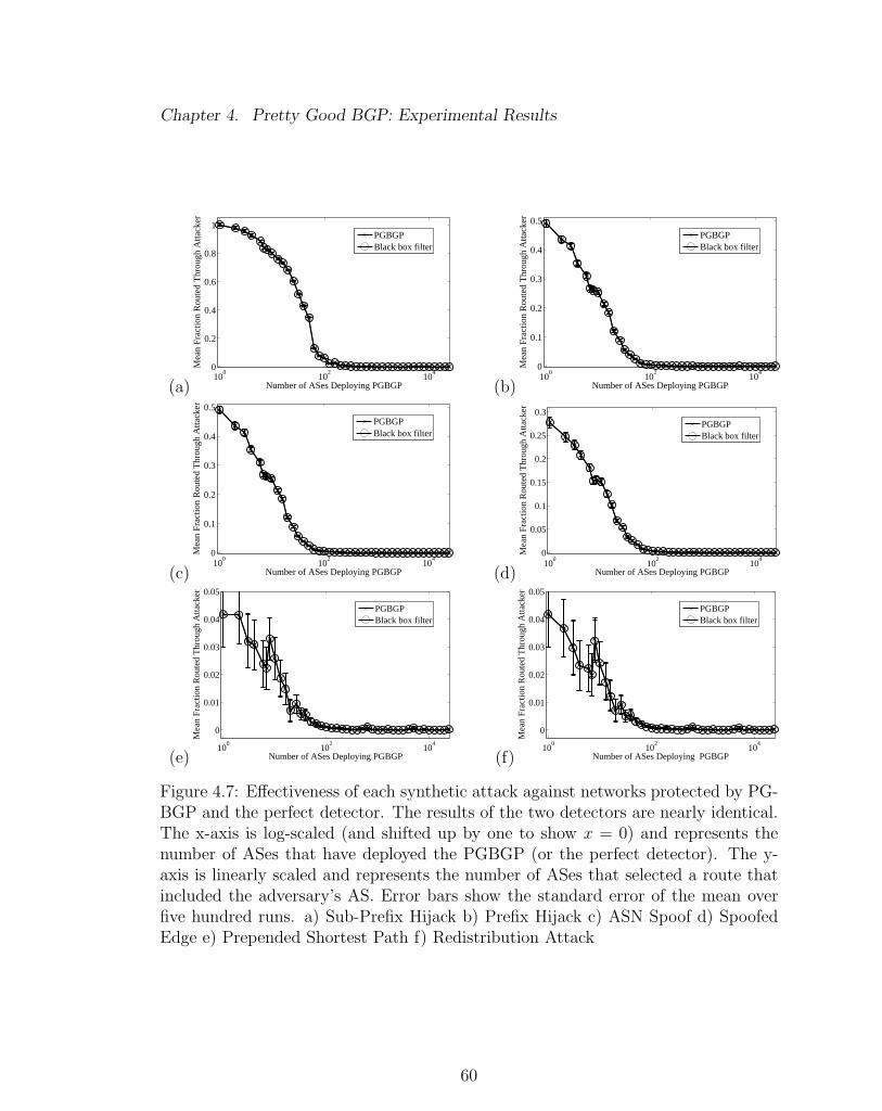
Chapter 4. Pretty Good BGP: Experimental Results
(a)10
010
210
40
0.2
0.4
0.6
0.8
1
Number of ASes Deploying PGBGP
Mea
n F
ract
ion
Rou
ted
Thr
ough
Atta
cker
PGBGPBlack box filter
(b)10
010
210
40
0.1
0.2
0.3
0.4
0.5
Number of ASes Deploying PGBGP
Mea
n F
ract
ion
Rou
ted
Thr
ough
Atta
cker
PGBGPBlack box filter
(c)10
010
210
40
0.1
0.2
0.3
0.4
0.5
Number of ASes Deploying PGBGP
Mea
n F
ract
ion
Rou
ted
Thr
ough
Atta
cker
PGBGPBlack box filter
(d)10
010
210
40
0.05
0.1
0.15
0.2
0.25
0.3
Number of ASes Deploying PGBGP
Mea
n F
ract
ion
Rou
ted
Thr
ough
Atta
cker
PGBGPBlack box filter
(e)10
010
210
4
0
0.01
0.02
0.03
0.04
0.05
Number of ASes Deploying PGBGP
Mea
n F
ract
ion
Rou
ted
Thr
ough
Atta
cker
PGBGPBlack box filter
(f)10
010
210
4
0
0.01
0.02
0.03
0.04
0.05
Number of ASes Deploying PGBGP
Mea
n F
ract
ion
Rou
ted
Thr
ough
Atta
cker
PGBGPBlack box filter
Figure 4.7: Effectiveness of each synthetic attack against networks protected by PG-BGP and the perfect detector. The results of the two detectors are nearly identical.The x-axis is log-scaled (and shifted up by one to show x = 0) and represents thenumber of ASes that have deployed the PGBGP (or the perfect detector). The y-axis is linearly scaled and represents the number of ASes that selected a route thatincluded the adversary’s AS. Error bars show the standard error of the mean overfive hundred runs. a) Sub-Prefix Hijack b) Prefix Hijack c) ASN Spoof d) SpoofedEdge e) Prepended Shortest Path f) Redistribution Attack
60

Chapter 5
Measuring and Modeling the
Autonomous System (AS) Level
Internet
This chapter describes work measuring and modeling the AS-level structure of the
Internet. In the first section, I measure the Internet’s AS-level structure from a radial
(from the core to the periphery) perspective. As discussed in Chapter 4, the Inter-
net’s topology is not well understood. Studying the AS-network’s structure helps
researchers to better understand the underlying mechanisms behind the network’s
growth. By studying the network from a radial perspective, it is possible to study
the core network apart from the periphery. Since the two portions of the network
have different functions (the core transits traffic for the periphery), it is important
to study them independently.
Statistical measurements of network structure can also be used to help validate
network growth models, to verify that the networks they produce are similar to the
real one. Network growth models are useful for testing network protocols on predicted
61

Chapter 5. Measuring and Modeling the Autonomous System (AS) Level Internet
future networks. They can also be used to ensure that protocols behave properly
on several instances of networks, not just a single inferred network. In Section 5.2,
I develop a model, called ASIM, capable of generating AS topologies. ASIM is the
first model to incorporate geography, economics, and traffic within a single frame-
work. The work in this chapter is a collaborative effort with Petter Holme 1 and is
published in the Proceedings of the Royal Society A [85] and SIGCOMM Computer
Communications Review [86].
5.1 Measuring the AS Network’s Topology
Since the turn of the century there has been increasing interest in the statistical
study of networks [87, 88, 89], stimulated in large part by the availability of large-
scale network data sets. One network of great interest is the Internet [90]. The
Internet is intriguing because its complexity and size preclude comprehensive study.
It is comprised of millions of individual end-nodes connected to tens of thousands of
ISPs whose relationships are continually in flux and only partially observable. One
way to cope with these complexities is by analyzing a single scale of Internet data, for
example, a local office network of computers and their inter-connections; a network
of email address book contacts; the network formed by URL links on the World Wide
Web; or the interdomain (Autonomous System) level of the Internet. This section is
concerned with the last of these examples—the AS graph. The vertices in the graph
are themselves computer networks; roughly speaking an AS is an independently
operated network or set of networks owned by a single entity. Edges represent pairs
of ASes that can directly communicate.
A major finding of earlier AS studies is that node degree (number of links to
1I gathered the data sets and helped develop the model while Petter implemented themodel and performed the statistical analysis
62

Chapter 5. Measuring and Modeling the Autonomous System (AS) Level Internet
other ASes) has a power law distribution [67]. The degree distribution is, however,
not the only structure that affects Internet dynamics [91]. Higher-order network
structures can also impact network dynamics. This section analyzes the AS graph
using methods that are appropriate for networks with a clear hierarchical organiza-
tion [90, 92]. In particular, I study network quantities as a function of the average
distance to other vertices. This approach allows us to separate vertices of different
hierarchical levels, in a radial (from core to periphery) fashion. This is, furthermore,
a way to determine how clearly separated the core and the periphery are. Most
analysis methods developed by physicists (degree frequencies, correlations, etc.) are
based on quantities averaged over the whole network and do not take a hierarchical
partitioning into account [90]. Studies by computer scientists, on the other hand,
assume a division of the AS level Internet into hierarchical levels [60]. I argue that
the observed AS level networks do have pronounced core-periphery dichotomy but
that the periphery has more structure than previously thought.
5.1.1 Networks
This subsection briefly reviews the organization of the AS-level Internet and de-
scribes the data sets. It also describes the network models that the observed data
is compared to. These models include one randomization scheme that samples ran-
dom networks with the same set of degrees as the original networks, the generative
Barabasi-Albert preferential attachment model [7], and the Inet model [71]. The null
hypothesis in these measurements is that the random networks accurately reflect the
Internet’s structure.
63
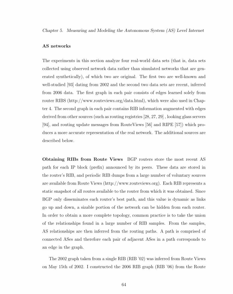
Chapter 5. Measuring and Modeling the Autonomous System (AS) Level Internet
AS networks
The experiments in this section analyze four real-world data sets (that is, data sets
collected using observed network data rather than simulated networks that are gen-
erated synthetically), of which two are original. The first two are well-known and
well-studied [93] dating from 2002 and the second two data sets are recent, inferred
from 2006 data. The first graph in each pair consists of edges learned solely from
router RIBS (http://www.routeviews.org/data.html), which were also used in Chap-
ter 4. The second graph in each pair contains RIB information augmented with edges
derived from other sources (such as routing registries [28, 27, 29] , looking glass servers
[94], and routing update messages from RouteViews [56] and RIPE [57]) which pro-
duces a more accurate representation of the real network. The additional sources are
described below.
Obtaining RIBs from Route Views BGP routers store the most recent AS
path for each IP block (prefix) announced by its peers. These data are stored in
the router’s RIB, and periodic RIB dumps from a large number of voluntary sources
are available from Route Views (http://www.routeviews.org). Each RIB represents a
static snapshot of all routes available to the router from which it was obtained. Since
BGP only disseminates each router’s best path, and this value is dynamic as links
go up and down, a sizable portion of the network can be hidden from each router.
In order to obtain a more complete topology, common practice is to take the union
of the relationships found in a large number of RIB samples. From the samples,
AS relationships are then inferred from the routing paths. A path is comprised of
connected ASes and therefore each pair of adjacent ASes in a path corresponds to
an edge in the graph.
The 2002 graph taken from a single RIB (RIB ’02) was inferred from Route Views
on May 15th of 2002. I constructed the 2006 RIB graph (RIB ’06) from the Route
64

Chapter 5. Measuring and Modeling the Autonomous System (AS) Level Internet
Views RIB on May 16th of 2006. The RIB ’02 graph has N = 13233 and M = 27724
while RIB ’06 has N = 22403 and M = 46343.
Extending the RIB Dataset There are other sources of AS connectivity data
besides Route Views. RIPE (http://www.ripe.net) has data collected from addi-
tional RIBs beyond those contained in the Route Views data. Peering information
is directly available for a small number of ASes that are participating Looking Glass
(http://www.traceroute.org) routers. Finally, some ASes register their peering rela-
tionships in regional registries such as RIPE. The extended 2002 AS graph (AS ’02)
was constructed using inferred topologies from all three of these sources, together
with the original Route Views data.
RIB data represent a brief snapshot of routing state. There are many paths that
a router sees only briefly, and the chances of capturing all of them from just a few
RIB dumps is unlikely. In the extended AS-graph of 2006 (AS ’06), I augmented
the Route Views RIB data with all of the paths found in BGP update messages
for the entire month of April 2006 from both Route Views and RIPE. This gives a
more complete picture over time, although it is still biased by the limited number of
routers from which the data were collected.
The extended 2002 AS-graph (AS ’02) has N = 13579, M = 37448 and the
corresponding 2006 network (AS ’06) has N = 22688 M = 62637. Thus the extended
data sets have 35% (2002) and 67% (2006) more edges than their RIB counterparts.
Null-model networks
To study the network structures beyond degree distribution I compare the AS net-
work data against a null model with the same degree distribution. The null model is
a random network constrained to have the same degree distribution as the original
65

Chapter 5. Measuring and Modeling the Autonomous System (AS) Level Internet
network. By comparing results for the observed networks with the same quantities
for the null model, we can observe additional network structure if it exists. One
way to sample a random network is to randomly rewire an existing graph so that
the degree distribution remains [95]. In my implementation I create a new random
network by enumerating the edges E of the original graph, and for each edge (i, j) I:
1. Choosing another edge (i′, j′) randomly and replacing (i, j) and (i′, j′) with
(i, j′) and (i′, j). If this creates a multi- or self-edge, then I revert to the
original edges (i, j) and (i′, j′), and repeating with a new (i′, j′).
2. Choosing two edges (i1, j1) and (i2, j2) and replacing them along with (i, j′) by
(i1, j′), (i, j2) and (i2, j1).
Step 2 guarantees ergodicity of the sampling [96], i.e. that one can go between any
pair of graphs with a given set of degrees by successive edge-rewirings.
Generative network models
In addition to the observed (inferred from data) and null-model networks described
above, I also study networks produced according to two previously proposed network-
generation schemes [7, 71]. The first is the well-known the Barabasi-Albert preferen-
tial attachment model [7]. The second, known as the Inet model, version 3.0 [71], is
more complex and designed specifically for creating networks with AS graph prop-
erties.
Both models are described in Chapter 2. Because the BA model has only one
integer parameter it is not very flexible at fitting data. In this document, I use
m = 3 to make the average degree as similar to the AS networks as possible. Other
preferential attachment models (e.g., [97]), can model the average degree and slope
of the degree distribution more closely. Such improvements, I believe, are unlikely to
66

Chapter 5. Measuring and Modeling the Autonomous System (AS) Level Internet
frac
tion
ofve
rtic
esfr
acti
onof
vert
ices
frac
tion
ofve
rtic
es
0.05
0.1
0.15
0.2
0
0.05
0.1
0.15
0.2
0
0.05
0.1
0.15
0.2
2 3 4 5 6 7average distance, d
2 3 4 5 6 7average distance, d
2 3 4 5 6 7average distance, d
(a)
(b)
(c)
AS ’02
RIB ’02
AS ’02 (null)
AS ’06
BA model
Inet model
AS ’06
RIB ’06
AS ’06 (null)
0
Figure 5.1: Normalized histograms of vertices with a specific average distance d tothe rest of the vertices. (a) shows curves for the Oregon Route Views data (RIB’02), extended data (AS ’02), and values for random networks with the same degreesequences as AS ’02. (b) displays curves for the Oregon Route Views data (RIB ’06),extended data (AS ’06), as well as randomized networks with the degree sequence ofAS ’06. (c) shows the same AS ’06 curve as (b) along with the BA and Inet modelresults for parameter values as close as possible to those of the AS ’06 network. 100averages were used for the null-model curves in (a) and (b) as well as the modelnetworks in (c). Lines are guides for the eyes. The error-bars represent standarderror (the point symbols are often larger than the error bars).
change the conclusions of Chapter 5 drawn from the original BA model. I use Inet’s
default parameter settings, except N which I extracted from the datasets, producing
an average degree that is approximately six.
5.1.2 Numerical results
This subsection presents the numerical results of the analysis. I first discuss the aver-
age distance metric for displaying network properties with a radial perspective. Then
67

Chapter 5. Measuring and Modeling the Autonomous System (AS) Level Internet
I define and present the results for each network structural measure as a function of
the average distance to other vertices.
Let d(i, j) denote the graph distance between two vertices i and j—the number
of edges in the shortest path between i and j. A simple measure for how peripheral
a vertex is in the network is its eccentricity—the distance to the most distant vertex,
maxj∈V d(i, j) [98]. Eccentricity is thus an extremal property of the network and is
determined by a small fraction of vertices. To reflect the typical path length of a
vertex I rank vertices according to an average property of the vertex. The average
property corresponding to eccentricity is the average distance from one vertex to all
of the others:
d(i) =1
N − 1
∑
j
d(i, j), (5.1)
where the sum is over all vertices, except i, in V . I note that the reciprocal value of
d(i), the closeness centrality, is a common measure for centrality in social network
studies [99, 98]. Average distance is a more intuitive measure in this context—
d(i) ≈ 2 means that i is on average two hops away from other vertices, whereas the
closeness value 0.5 does not have such a direct interpretation.
Another way to study eccentricity is by iteratively removing vertices of low-
degree to construct a sequence of k-cores (subgraphs in which all vertices have degree
≥ k) [60, 100]. In this study, the average distance metric is used instead because it
measures separation of vertices. Further, because it is a global measure (in the sense
that the entire network topology affects d(i) for every i) it is likely more robust to
errors in the input data.
Peering policies do not always allow each router to pick the shortest topological
path to every destination. For instance, a route learned through a customer might
be longer than through a peer-to-peer link but as it would provide revenue, policy
demands that the customer route be used. Therefore the d(i) values shown in this
68

Chapter 5. Measuring and Modeling the Autonomous System (AS) Level Internet
chapter do not always represent valid routing paths. More accurate measurements
would require relationship information which is difficult to attain because these data
are often treated as proprietary and inferencing methods are inaccurate.
Radial vertex density
The fraction of vertices as a function of d are shown in Fig. 5.1.2. The figure shows
the distribution of d for my data sets and the AS graphs produced by the BA and Inet
models. The observed networks produce graphs that are far from smooth, unimodal
distributions. Instead they have one peak close to d = 3, a smaller peak around
d = 4, and for the 2006 data, a third peak near d = 5. The difference between
the RIB-only and the extended datasets is small, except around the second peak
in Fig. 5.1.2(b) which is higher in the RIB-only data. The null-model curves are
much more unimodal, although they do not follow a simple, smooth functional form.
Such a unimodal form could be a result of the averaging of many null-model curves,
but the observation holds even if single realizations of the randomization are plotted
(data not shown). Thus, the observed AS graph is less homogeneous than what I
would predict by considering only vertex degree.
The two peaks can be interpreted as an effect of the hierarchical organization
of the Internet. The core (Tier-1 providers and other large ISPs) is in the low-d
tail, the d = 3 peak are vertices directly connected to the core, and the d = 4
peak are vertices whose closest neighbors are in the d = 3 peak. This explains the
approximately integer distance between the peaks. As expected, the Tier-1 ASes
(AS numbers 209, 701, 1239, 1668, 2914, 3356, 3549, 3561, 6461 and 7018 in the
data sets) have an average d = 2.35± 0.03 in the AS ’02 data and d = 2.41± 0.03 in
the AS ’06 data, and are thus in the center of the network (left of the most central
peak). Thus, the Tier-1 ASes are in the extreme low end of the d-spectrum.
69
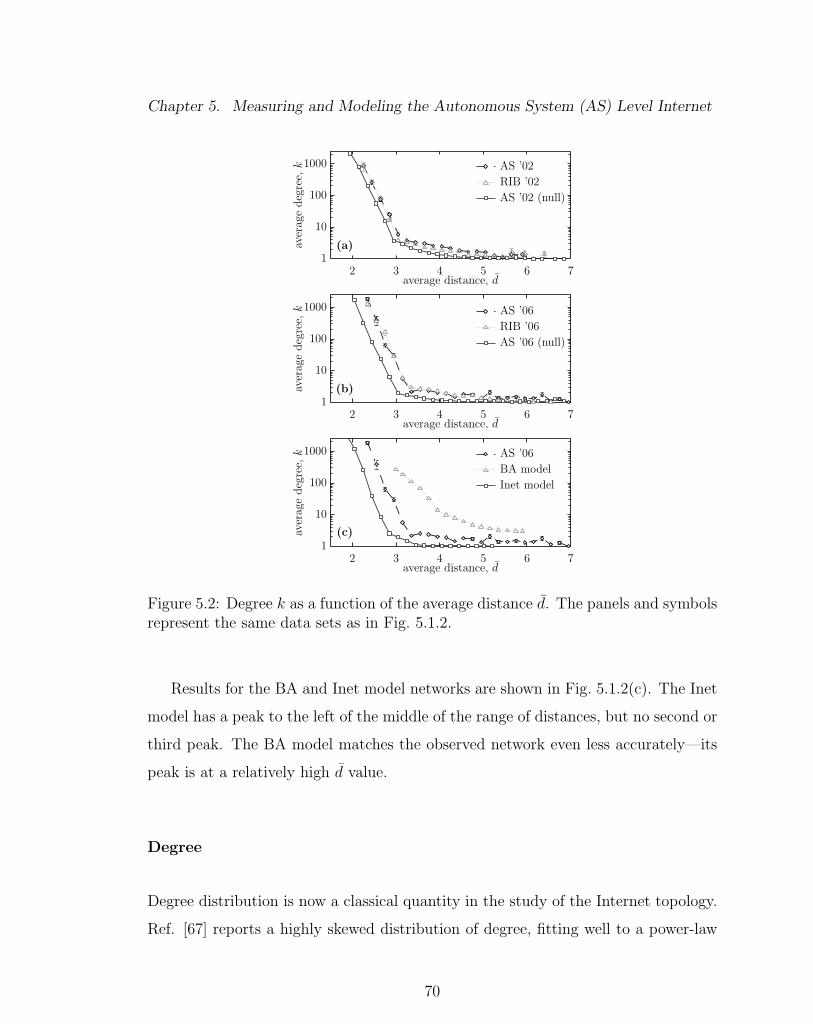
Chapter 5. Measuring and Modeling the Autonomous System (AS) Level Internet
(b)
(c)
(a)
AS ’06
BA model
Inet model
AS ’06
RIB ’06
AS ’06 (null)
AS ’02
RIB ’02
AS ’02 (null)
aver
age
deg
ree,
kav
erag
edeg
ree,
kav
erag
edeg
ree,
k
1
10
100
1000
2 3 4 5 6 7average distance, d
1
10
100
1000
2 3 4 5 6 7average distance, d
1
10
100
1000
2 3 4 5 6 7average distance, d
Figure 5.2: Degree k as a function of the average distance d. The panels and symbolsrepresent the same data sets as in Fig. 5.1.2.
Results for the BA and Inet model networks are shown in Fig. 5.1.2(c). The Inet
model has a peak to the left of the middle of the range of distances, but no second or
third peak. The BA model matches the observed network even less accurately—its
peak is at a relatively high d value.
Degree
Degree distribution is now a classical quantity in the study of the Internet topology.
Ref. [67] reports a highly skewed distribution of degree, fitting well to a power-law
70

Chapter 5. Measuring and Modeling the Autonomous System (AS) Level Internet
with an exponent around 2.2. Since this finding, the degree distribution has become
a core component in models of the AS graph—both the BA and Inet models as
well as others [68, 69, 70] create networks with power-law degree distributions. One
interpretation of degree is that it is a local centrality measure [98]. Further, different
measures of centrality are known to be highly correlated [101, 102, 103] so one can
expect the average degree k to be a decreasing function of the average distance d.
Figure 5.2 confirms this prediction for both the observed and model networks.
In Fig. 5.2(a) and (b) I observe that the k(d)-curves decrease dramatically until the
approximate location of the first peak in the distribution plots Fig. 5.1.2(a) and (b).
Therefore, d identifies a natural border between the core vertices of high-degree and
low average distance, and the sparsely connected periphery. The observed graphs,
however, have higher degree in the periphery compared to the null-model curves.
This suggests that the network periphery may have more complex wiring topology
than that is predicted by degree distribution alone. This pattern occurs in the other
network measurements as well.
The Inet model (Fig. 5.2(c)) fails to capture the higher degree (implying addi-
tional complexity) in the periphery. Because the BA model has a minimal degree
of three, it is difficult to compare to the observed networks. However, the decrease
of the k(d)-curves at the largest d-peak is not conspicuous in the BA model curves.
Thus, there is no clear core-periphery dichotomy in the BA model. This too is not
surprising, because the BA model was designed to produce “scale-free” networks in
the sense of fractals (if one zooms in on any part of system, it looks similar to the
whole).
71

Chapter 5. Measuring and Modeling the Autonomous System (AS) Level Internet
(a)
(b)
(c)AS ’06
BA model
Inet model
AS ’06
RIB ’06
AS ’06 (null)
AS ’02
RIB ’02
AS ’02 (null)
1
10
100
1000
1
10
100
1000
1
10
100
1000
2 3 4 5 6 7average distance, d
2 3 4 5 6 7average distance, d
2 3 4 5 6 7average distance, d
nei
ghbor
deg
ree,
Knei
ghbor
deg
ree,
Knei
ghbor
deg
ree,
K
Figure 5.3: Neighbor degree K as a function of the average distance d. The panelsand symbols represent the same data sets as in Fig. 5.1.2.
Neighbor degree
Degree is a property of individual vertices, with no information about how they are
interconnected. In this sense degree is a measure of local network structure. To un-
derstand the network’s non-local organization [104], one can measure the correlations
of degrees between neighbors in the network. There are three common approaches.
The first, known as assortative mixing coefficient [89], measures the Pearson correla-
tion coefficient for each edge. This provides one number for the entire network and
is thus appropriate for comparisons between networks. The second approach makes
a density plot that displays the fraction of edges with degree (k1, k2). This kind of
72

Chapter 5. Measuring and Modeling the Autonomous System (AS) Level Internet
two-dimensional plot is called a correlation profile [105, 106]. Correlation profiles
provide more detailed information than the assortative mixing coefficient, but they
are less concise and more sensitive to noisy data. The third approach measures
average neighbor degree
K(i) =1
k(i)
∑
j∈Γi
k(j) , (5.2)
(where Γi is the neighborhood of i) as a function of degree k(i) [97]. All approaches
must be compared to null models because skewed degree distributions are known to
induce negative-correlations [105]. The third approach produces a one-dimensional
plot and thus forms a middle ground between the assortative mixing coefficient and
the correlation profile. It is also a method that can be adapted to the radial-plot
framework—by plotting K against d one can monitor the correlation between cen-
trality and neighbor degree. For the AS-level Internet high-degree vertices are, on
average, connected to vertices of low degree and vice versa [97]. Since degree de-
creases with d, one would then expect K to be an increasing function of d.
As seen in Fig. 5.3, vertices at intermediate distances have neighbors of highest
degree. The peak in K(d) coincides with the largest peak in the histograms found
in Fig. 5.1.2, and the change of slope in Fig. 5.2. This suggests that the periphery is
composed of two levels: the intermediate majority which is primarily connected to
the core, and the extreme periphery that is connected to other periphery vertices.
It is also apparent in Fig. 5.3(a) and (b) that the null-model qualitatively has the
same shape as the observed network; but, just as for degree distribution; neighbor
degree values are larger in the observed networks than the null-model. Also, the Inet
model underestimates the average neighbor degree in the periphery. Finally, the BA
model exhibits less correlation between K and d.
73

Chapter 5. Measuring and Modeling the Autonomous System (AS) Level Internet
AS ’02
RIB ’02
AS ’02 (null)
AS ’06 AS ’06 (null)
RIB ’06
AS ’06
BA model
Inet model
(b)
(c)
(a)10−6
10−5
10−4
10−3
0.01
del
etio
nim
pac
t,φ
10−6
10−5
10−4
10−3
0.01
del
etio
nim
pac
t,φ
10−6
10−5
10−4
10−3
0.01
del
etio
nim
pac
t,φ
2 3 4 5 6 7average distance, d
2 3 4 5 6 7average distance, d
2 3 4 5 6 7average distance, d
Figure 5.4: Deletion impact φ as a function of the average distance d. The panelsand symbols represent the same data sets as in Fig. 5.1.2.
Deletion impact
If a vertex is not actively routing packets due to fault or attack, other vertices might
be affected. I am interested in knowing how susceptible a given network structure
is to random node failures. Assuming that the network is connected, let Si be the
number of vertices in the largest connected subgraph after the deletion of i. I define
the deletion impact as
φ(i) =N − 1− Si
N − 2. (5.3)
74

Chapter 5. Measuring and Modeling the Autonomous System (AS) Level Internet
This measure can take values in the interval [0, 1]. A value of 0 means that the entire
network, except i, is still connected after the deletion. A value of 1 means that all of
the network’s edges were attached to i and that all of the vertices are isolated after
the deletion.
Fig. 5.4 plots deletion impact as a function of the average distance for the same
data sets as the previous figures. All curves are roughly decreasing. This means that
the network is more sensitive to the deletion of central, than peripheral, vertices. This
observation is anticipated from earlier studies showing that the Internet is vulnerable
to targeted attacks at the vertices of highest degree [107] but robust to random
failures. This is because the majority of vertices have low φ-values. However, the
deletion impact measure can detect more subtle effects in the periphery.
The first peak in the d-distribution is, as mentioned above, around d = 3. At
this distance φ has decreased a thousand times from the core where φ ∼ 10−2.
In this quantity I see a substantial difference from the null-model; the peripheral
vertices of the inferred networks have significantly lower deletion impact than the
peripheral vertices of the null-model networks. This, I believe, is another effect of the
high degree of peripheral vertices. The fact that the periphery is relatively highly
connected suggests that there are alternate routes that could be used if a regular
path is obstructed by a vertex failure. In the case of the Inet model, which has very
few vertices of high d, the peripheral φ values are quite low because the periphery is
well connected to the core. As expected, φ = 0 for all vertices in the BA model since
all vertices have degree of at least three. The BA model thus produces network that
are more robust to vertex deletion than the observed networks are.
75

Chapter 5. Measuring and Modeling the Autonomous System (AS) Level Internet
(b)
(c)
(a)
AS ’06
BA model
Inet model
AS ’06
RIB ’06
AS ’06 (null)
AS ’02
RIB ’02
AS ’02 (null)
0
0.05
0.1
0.15
0.2
clust
erin
gco
effici
ent,
C
0
0.05
0.1
0.15
0.2cl
ust
erin
gco
effici
ent,
C
0
0.05
0.1
0.15
0.2
clust
erin
gco
effici
ent,
C
2 3 4 5 6 7average distance, d
2 3 4 5 6 7average distance, d
2 3 4 5 6 7average distance, d
Figure 5.5: Clustering coefficient C as a function of the average distance d. Thepanels and symbols represent the same data sets as shown in Fig. 5.1.2.
Clustering coefficient
The clustering coefficient C(i) [108] is another frequently studied network property:
C(i) = M(Γi)/(
k(i)
2
)
(5.4)
M(X) denotes the number of edges in a subgraph X. The clustering coefficient
measures how interconnected the neighborhood of a vertex is. One interpretation
is that C(i) is the number of connected neighbor pairs rescaled by the theoretical
maximum. C(i) can also be seen as the fraction of triangles that i is a member of,
normalized to the interval [0, 1].
76

Chapter 5. Measuring and Modeling the Autonomous System (AS) Level Internet
In Fig. 5.5 I display the clustering coefficient as a function of the average distance.
The curves for the observed graph, null-model, and Inet model networks show a peak
around the same point as the peak in the d-distribution. However, the null-models do
not exhibit as high a degree of clustering in the periphery as the inferred networks.
In other words, there are more triangles in the periphery than can be expected from
only the network’s degree distribution. In fact, for 100 null-model networks based on
the AS ’06 network, no triangles existed for d > 3.8 with any vertex having d > 3.8.
This should be compared with 1124 triangles for the AS ’06 network itself (there are
even 83 triangles where all vertices have d > 3.8). This further suggests that the
periphery of the observed AS graphs is complex. As triangles represent redundancy
(the three vertices will still be connected if any one of the edges are cut) this could
help to explain the increased robustness to deletion seen in Section 5.1.2. As seen
in Fig. 5.5(b), neither the Inet, nor the BA model predict a significant number of
peripheral triangles. The low deletion impact values for peripheral vertices in these
models may be attributed to the presence of longer cycles.
Distance balance
In the context of scientific collaboration networks it has been shown [109] that the
number of shortest paths leaving a vertex via a specific neighbor is skew distributed
(asymmetric). In other words, most of the shortest paths from a vertex i to the rest
of the network traverse a single neighbor of i. To rephrase this in terms of the average
distance, central vertices are likely to have few neighbors with smaller d values. This
leads us to another view of centrality. Let the distance balance of b(i) be the fraction
of i-neighbors j with d(j) < d(i). Clearly one can expect this to be an increasing
function of d, but is it a linear increase?
Figure 5.6 plots the distance balance as a function of d. As expected, all of the
curves generally increase but not linearly. Almost all the increase from 0 to 1 takes
77

Chapter 5. Measuring and Modeling the Autonomous System (AS) Level Internet
(b)
(c)
(a)
AS ’06
BA model
Inet model
AS ’06
RIB ’06
AS ’06 (null)
AS ’02
RIB ’02
AS ’02 (null)0
0.2
0.4
0.6
0.8
1
dis
tance
bal
ance
,b
0
0.2
0.4
0.6
0.8
1dis
tance
bal
ance
,b
0
0.2
0.4
0.6
0.8
1
dis
tance
bal
ance
,b
2 3 4 5 6 7average distance, d
2 3 4 5 6 7average distance, d
2 3 4 5 6 7average distance, d
Figure 5.6: Distance balance b as a function of the average distance d. The panelsand symbols represent the same data sets as shown in Fig. 5.1.2.
place around the highest peak in Fig. 5.1.2, which gives another characterization of
the core and periphery: in the core, the typical vertex has relatively few neighbors of
higher centrality than itself (and vice versa in the periphery). The b(i) values in the
peripheral region of all curves approach values close to 1. In Fig. 5.6(b) the curves of
the observed data are somewhat lower. This supports the previous observation that—
as seen previously in quantities such as degree, neighbor degree, and the clustering
coefficient—the periphery is structurally less different from the core than what can be
expected from random networks constrained to the degree sequence of the observed
networks. As seen in Fig. 5.1.2(c), the Inet model behaves like the null-model—
78

Chapter 5. Measuring and Modeling the Autonomous System (AS) Level Internet
the same observation holds for the average neighbor degree (Fig. 5.3) and clustering
coefficient (Fig. 5.5). Unlike the Inet model, the BA model’s curve increases more
smoothly which suggests (in accordance with what has been observed above) a less
pronounced core-periphery structure than the observed networks.
5.1.3 From Measurement to Modeling
This section has discussed a number of statistical measurements (beyond node de-
gree) that can be used to study the AS-graph. The next section builds upon this
work to generate graphs that are shown to be statistically similar to the real AS
graph.
5.2 Modeling the AS-Level Internet
This section describes an agent-based model capable of creating networks similar to
the AS network. Since the actual AS network is difficult to uncover, as discussed
in Chapter 4, it is useful to generate Internet-like networks that can be used to test
protocols are a large number of graphs for validation.
As one of the most complex human artifacts, the Internet is a challenging system
to model. Dynamic processes of different time scales operate simultaneously—from
slow processes, like the development of new hardware to the transport of data, which
often occurs at the speed of light.
These phenomena are to some extent interdependent. Traffic provides income
to the service providers, which is then invested in infrastructure, which can lead to
changes in traffic patterns. This section describes a mechanistic, agent-based model
(ABM) [110] to study how these phenomena interact to produce the macroscopic
79

Chapter 5. Measuring and Modeling the Autonomous System (AS) Level Internet
features of the Autonomous System (AS) level Internet. Instead of simply repro-
ducing a macroscopic pattern using statistical fitting or phenomenological models,
mechanistic models specify a set of primitive components (known as agents) and in-
teraction rules that mimic the architecture of the real system. The models are judged
on their ability to generate realistic macroscopic behaviors from these primitive com-
ponents. The goal is to provide a parsimonious explanation of how a system works
by hypothesizing a small set of simple but relevant mechanisms. In this spirit my
model attempts to reproduce large-scale features of the Autonomous System level of
the Internet by modeling localized and well-understood network interactions.
The ASes of the Internet lend themselves naturally to ABM modeling. Each AS
is an economic agent, comprised of a discrete network that can have spatial extent.
Over time, ASes create new links to other ASes, upgrade their carrying capacity,
and compete for customer traffic. The agents in the model described here, behave
similarly, although in simplified way. The model is designed to be general enough
to simulate any spatially extended communication network built by subnetworks of
economically driven agents.
In previous work, Chang et al. showed that incorporating economics and geogra-
phy into the Highly-Optimized Tolerance (HOT) [111] model increases the model’s
accuracy [112]. A related ABM model of the AS graph produces degree distributions
similar to empirical observations [113]. Bar et al. proposed a similar model [114]
that incorporates another aspect of the real Internet—that the agents are spatially
extended objects. My model is similar in scope to this earlier work but differs in the
details, most importantly by adding explicit economics in the form of cost. Other
differences include accounting for population density, simplifying the treatment of
traffic flow, and not assuming a HOT framework. The previous work in this area,
like much research on network models, focuses almost exclusively on degree distri-
butions of the graphs. This subsection compares the model’s output to Internet
80

Chapter 5. Measuring and Modeling the Autonomous System (AS) Level Internet
data using several topological measures [85], including degree distributions, as well
as geography and traffic dynamics.
The remainder of this chapter is organized as follows. First, I describe and
motivate the model. Then, I characterize the time evolution, network topology,
correlation between network structure and traffic flow, packet routing statistics, and
geographical aspects of the networks produced by the model. Where possible, I
compare the properties of these synthetic networks to observed data from the Internet
(such as that shown in Section 5.1).
5.2.1 AS Simulation Model (ASIM)
I begin with the fundamental unit responsible for network growth, an agent with
economic interests [115]. These agents manage traffic over a geographically extended
network (which I refer to as a sub-network to distinguish it from the network of ASes)
and profit from the traffic that flows through their network.
This section compares agents to the ASes that comprise the Internet. This is
not an exact mapping—some of the Internet Service Providers (ISPs) have many
AS numbers (e.g., AT&T), while other ASes are shared by several organizations.
ASIM makes the common simplifying assumption that once an agent is introduced,
it does not merge with another agent or go bankrupt [90, 116, 113]. This is partially
justified by the fact that the Internet, from its inception, has grown monotonically,
and the model tries to capture this dynamic. Most models of the AS graph enforce
strict growth [90] as well and are justified by their a posteriori ability to reproduce
measured features.
The model assumes a network user population distributed over a two-dimensional
area. Traffic is simulated by a packet-exchange model, where a packet’s source and
destination are generated with a probability that is a function of the population
81

Chapter 5. Measuring and Modeling the Autonomous System (AS) Level Internet
a b c
Figure 5.7: Illustration of the network growth algorithm: (a) shows the locations offour agents on the geographic grid. These are assumed to be connected by a physicalnetwork administrated by the agent, but this assumption is not explicit in the model.(b) Example graph resulting from (a). Illustrates that two agents are present in thesame pixel is a necessary, but not sufficient condition for a link to form between theagents. (c) Illustrates the area that each hypothetical agent can afford to expand to(the shaded region).
profile. The model is initialized with one agent comprised of a network (a sub-
network in my terminology) that spans one grid location (referred to as a pixel of the
landscape. As time progresses, the agent may extend its subnetwork to other pixels,
so that the sub-networks reach a larger fraction of the population. This creates
more traffic, which generates profit, which is then reinvested into further network
expansion. Through positive feedback, the network grows until it covers the entire
population. This subsection describes the assumptions and most of the details of the
model; the source code is publicly available from www.csc.kth.se/∼pholme/asim/.
An agent i is associated with a set of locations Λi (representing sources or end-
points of traffic, and peering points), a capacity Ki (limiting the rate of packets that
can pass through the agent), a packet-queue Qi, and a set of neighbor agents Γi. A
necessary, but not sufficient, condition for two agents to be connected is that their
locations overlap in at least one pixel. The locations exist on an Lx × Ly square
grid. A pixel of the grid is characterized by its population p(x, y) and the set of
agents with a presence there A(x, y). The total number of agents in the simulation
is denoted by n, and the number of links between agents by m. These quantities,
82

Chapter 5. Measuring and Modeling the Autonomous System (AS) Level Internet
except Lx and Ly, depend on the simulation time. The outer loop of the model then
iterates over the following steps:
1. Network growth. The number of agents is increased. Existing agents expand
geographically, and their capacities are adjusted.
2. Network traffic. Packets are created, propagated toward their targets, and
delivered. This process is repeated Ntraffic times before the next network-growth
step.
I measure simulation time τ as the number of times Step 1 is executed (the time
unit between packet movements is 1/Ntraffic). In the remainder of this subsection I
describe the growth and traffic steps in greater detail.
Network growth
The income of an agent, during a time step, is proportional to the traffic propagated
by the agent during the period. This is a simplification. For example, income could
depend both on the amount of traffic and the prices for forwarding the packets set
by business agreements. Assume an agent i has a budget Bi that it invests so that it
can increase its traffic, and thus its profit. Since there is a possibility of congestion
in the model, agent i tries first to remove bottlenecks by increasing its capacity Ki
(the number of packets that the agent can transit during one time step). When the
capacity is sufficient, the agent spends the rest of its budget on increasing its traffic
by expanding geographically. There are three prices associated with network growth.
The capacity price Ccapacity is the price of increasing Ki one unit. For simplicity I let
Ccapacity be independent of the size of the agent’s subnetwork. The wire price Cwire is
the price per pixel between a new location and the agent’s closest existing location.
Finally, Cconnect is the cost of connecting two agents with locations at the same pixel.
83

Chapter 5. Measuring and Modeling the Autonomous System (AS) Level Internet
The average degree (number of neighbors of an AS) in the AS graph has been
relatively constant over time [90, 117] (increasing about 5% from 2001 to 2007).2 I
take this as a constraint in the model and let the desired average degree kD be a
control parameter. I also assume that each agent tries to spend all of its budget, but
not more than that, whenever it is updated.
The network growth step iterates over the following steps:
1. Increase of the number of agents. As long as the network is too dense (i.e. if
2m > kDn), new agents are added. New agents are situated in the pixel (x, y)
that has the highest available population p(x, y)/(A(x, y) + 1) where A(x, y)
is the cardinality of A(x, y) and A(x, y) ≥ 1. The budget and capacity of the
new agents are initialized to Binit and Kinit respectively.
If the network is small, n < kD + 1, it is not dense enough for new agents to
be added in step 1. Thus, I do not apply this condition when n is less than a
threshold n0 and call the time when n = n0 is reached t0.
2. Capacity increase. Each agent synchronously increases its subnetwork’s capac-
ity based upon traffic from the last time step (but not more than the agent
can afford). Agent i invests the minimum of (Bi, Ccapacity∆Ti, 0, 0) to increase
capacity (∆Ti is the change in traffic propagated by i since the last update).
3. Link addition. While 2m ≤ nkD (which usually means kD − 1 times), choose
two agents randomly that are not already connected and share a common pixel.
If the budgets of both agents are larger than Cconnect, then connect them.
4. Spatial extension. Let the agents with remaining budget extend their networks.
Iterate through all agents i and add a location at the pixel, not in Λi, that has
2This calculation is based on data from Oregon Route Views, www.routeviews.org.Although more edges of the AS graph can be identified by combining multiple data sources,the Route Views data set has been compiled in a consistent way over the years, so I believethat the relative degree increase is reliable.
84

Chapter 5. Measuring and Modeling the Autonomous System (AS) Level Internet
t
s
b
a
t = 2 t = 3t = 1
Figure 5.8: Illustration of traffic simulation. (a) A packet is created with source pixels and target pixel t with probability proportional to the product of populations at sand t. One of the agents at the target pixel is randomly chosen as the target agent.The propagation of the packet is shown in the graph. Each agent i is associatedwith a queue Qi and a capacity Ki. When a packet reaches an agent, it is appendedto Qi. Ki packets in the queue are relayed to neighboring agents and i’s budget iscredited one unit. The arrows in (b) symbolize the packet’s route from source todestination agent. The package is routed to a neighboring agent j with probabilityexp((d(i, t)−d(j, t))/λ (where t is the packet’s target, d(·, ·) gives the graph distance,and λ is a parameter).
the highest available population p(x, y)/(L(x, y) + 1), and is not further than
(Bi − Cconnect)/Cwire from a location in Λi (i.e., not further from i than i can
afford). (See Figure 5.7(b)). Alternatively, the algorithm could select the
point with the lowest cost per unit of population. However, such an algorithm
is computationally prohibitive for studying networks of the Internet’s scale.
Each agent’s budget is updated immediately after each modification.
85

Chapter 5. Measuring and Modeling the Autonomous System (AS) Level Internet
Network traffic
I model traffic with a discrete, packet-exchange model [118, 119]. The packets are
generated with specific source and target pixels, but the routing takes place on
the network of agents. I neglect intradomain routing among the agent’s locations,
assuming that the time it takes for a packet to pass through an agent is independent
of the specific locations it visits. The dynamics are defined as follows:
1. Packet generation. I assume that most traffic originates from direct communi-
cation between individuals and does not depend on the distance between them.
For each pair of points [(x, y), (x′, y′)] on the grid, I create a packet with source
(x, y) and destination (x′, y′) with probability Ppkg p(x, y) p(x′, y′), where Ppkg
is a parameter that controls the rate at which new packets are created. Then,
an agent is selected at random from those at the source pixel to become the
source node. The destination agent is randomly chosen from the agents at the
destination pixel. Finally, one unit of credit is added to the sender’s budget.
2. Packet propagation. Each agent i propagates the first Ki packets from its queue
(of length li) each time step and receives one unit credit for each propagated
packet. A packet can travel only one hop (inter-AS transmission) per time step.
A packet at agent i is propagated to a neighbor j with probability exp(λ(d(i, t)−
d(j, t)) (where t is the recipient AS, d( · , · ) is the graph distance, and λ is a
parameter controlling the deviation from shortest-path routing [120] observed
in Ref. [121]).
3. Packet delivery. For all agents, delete all packets that have reached their target.
The assumption in step 1 that the probability of two agents communicating is
independent of their spatial separation agrees with the (somewhat debated) “death
of distance” in the Internet age [122]. I also tested communication rates that decay
86

Chapter 5. Measuring and Modeling the Autonomous System (AS) Level Internet
with the square of the distance, as observed in conventional trade firms [123], with
qualitatively similar results. ASIM’s traffic propagation model is simplified from
reality, and it more closely resembles peer-to-peer traffic than user-to-service traffic.
The model also assumes that temporal fluctuations in packet generation are negligible
and ignore peak levels of congestion. Because the economy of the agents grows as
function of accumulated traffic through their subnetworks, average traffic load is a
reasonable approximation. Given the level of abstraction in my model, I believe
these traffic propagation assumptions are reasonable.
Business agreements between ASes are an important factor in BGP [20]. Next
hops are often selected by cost, rather than path length, which inflates the average
path length as shown in [121]. Although inter-AS contractual agreements are not
explicitly included, probabilistic propagation method 2 has a similar effect on average
path length.
5.2.2 Numerical simulations
Parameter values
Before presenting the simulation results, this sub-section describes the experimental
design, and choice of parameters. First, it specifies a population profile p(x, y), pri-
marily modeled from population distributions but one experiment involves a specific
geographic population (U.S.A census data). To simplify the generation of popula-
tion distributions, I neglect spatial correlations and simply model the frequency of
population densities. This frequency has two important features: it is skewed (pix-
els with low population densities are more frequent than highly populated pixels)
and fat-tailed (there are pixels with a population density many orders of magni-
tude larger than the average). One probability distribution with such features is the
power-law distribution Prob p ∼ p−χ. To reduce the fluctuations between different
87
Chapter 5. Measuring and Modeling the Autonomous System (AS) Level Internet
Parameter Interpretation ValueLx = Ly Number of pixels in the x (and y) direction 50Ntraffic Number of packets sent per simulation step 1× 10⁴
Ppkg Constant to determine packet source and dest. 0.001n0 Agent growth threshold 35
Kinit Initial capacity of an agent 5Cwire Price per pixel for new wire 500Binit Initial budget for a new agent 3× 10⁵
λ Parameter in exponential distribution 75
Table 5.1: Default parameters values for simulation experiments.
realizations of {p(x, y)}, and prevent unrealistically high populations within a pixel,
I sample the power-law distribution in the bounded interval [1, (LxLy)1/(1−χ)] [124]
with χ = 3. The results do not depend strongly on the distribution of p(x, y). Qual-
itatively similar results are obtained with normally distributed p values and real
population-density maps (data not shown).
In multi-parameter, agent-based models, such as ASIM, a systematic investigation
of the full parameter space is infeasible. Parameters are, if possible, obtained from
real systems. I set the desired degree kD = 5.52, the same average degree reported
in Ref. [85]. Unless otherwise stated, the desired size of the network is nD = 16,000,
which is the same order of magnitude as the current AS graph. Other parameters
are balanced to keep runtime low (less than one day) while still engaging all aspects
of the algorithm. This means, for example, that between every network update,
a significant number of packets are routed through even the smallest agents, and
enough packages to cause congestion pass through larger agents. Unless otherwise
stated, the experiments use the parameter set given in Table 5.1. Many of the
results are taken from a single run, but the results are shown to be representative by
comparing them to 20 other runs.
88

Chapter 5. Measuring and Modeling the Autonomous System (AS) Level Internet
ca
b
frac
tion
n,m 〈τp〉
〈d〉100
1000
104
2.5
3
3.5
4
〈τp〉,〈d〉
0
0.25
0.5
0.75
1
104
number of agents,n
number of links,m
covered population
time,τ ×1061 1.5 2 2.5
1000100×106
1 1.5 2 2.5time,τ number of agents,N
covered area
Figure 5.9: Time evolution of an example run. In panel (a) the number of agents andthe number of inter-agent links is shown as a function of simulation time. In (b) thefraction of the landscape with network coverage, and the fraction of the populationreached by the network, is plotted against time. Panel (c) shows the average traveltime 〈τp〉 for packets and the average distance (number of inter-agent hops) in thenetwork 〈d〉, as functions of the number of agents.
Network Growth
This sub-section studies the growth of the network over time. Fig. 5.9(a) plots the
number of agents and links as a function of simulation time for one representative
run. At τ = τ0 ∼ 4 × 10⁵ the graph is sparser than kD. Initially, the agents spend
their budget on new links and increasing capacity. At τ ∼ 1.5 × 10⁶, the budget of
the wealthier agents is sufficient to invest in wires to new locations (see Fig. 5.9(b)).
This creates new traffic, which causes positive feedback accelerating the traffic flow,
coverage, budget, and also more congestion. At τ ∼ 1.9×10⁶, n(τ) and m(τ) change
from exponential to sub-exponential growth. As seen below, this is also the time when
a significant level of congestion appears in the network. At about the same time,
the network has expanded to serve entire population. With the current model, the
network would continue to grow indefinitely with decreasing returns for the agents. A
plausible extension would be to introduce maintenance costs that are proportional to
network size, in which case the network would reach a steady state where the budgets
89

Chapter 5. Measuring and Modeling the Autonomous System (AS) Level Internet
of the agents are balanced and no further investments can be made. For τ & 1.9×10⁶
the increase of n(τ) is slower than exponential. This is explained by the increasing
level of congestion in the system. Figure 5.9(c) plots the average time 〈τp〉 for a
packet to travel from source to destination. 〈τp〉 is bounded from below by the average
distance (number of links in the shortest path, averaged over pairs of nodes) 〈d〉. The
two curves diverge, i.e. a significant level of congestion appears, around N = 1000.
The growth of n(τ) and m(τ) slows down at the same point. The slowing in growth
likely arises from a congestion-driven negative feedback. The most striking feature
of network growth over time is the transition from a small network, almost constant
in size, to a rapidly increasing system (around τ ∼ 1.8× 10⁶). This effect is typical
for technologies emerging from the interactions of a large number of agents—they
need a critical mass of users to reach a significant fraction of the total population.
One can argue that the Internet reached this critical mass in the early 1980’s when
it started to span the globe. Another important point in the Internet’s history
was the advent of the World Wide Web (WWW) in the early 1990’s, and with it
commercial applications and access to the general public. My model does not include
applications, such as the WWW, that undeniably affect network growth. Such effects
could be included by adopting a different traffic model, but for this chapter I aim
at simplicity and generality. In the Internet, ASes growth has been slower than
the exponential increase of agents predicted by the model (bgp.potaroo.net/cidr/;
read January 7, 2008). This discrepancy arises in part because the model does
not assume that maintenance costs are proportional to income. For example, if
maintenance costs grew super-linearly, then negative feedback could dampen growth.
Other external factors, such as the centralized method for allocating and assigning AS
numbers (Internet Assigned Numbers Authority, www.iana.org), might also influence
the actual rate of growth experienced by the Internet.
90

Chapter 5. Measuring and Modeling the Autonomous System (AS) Level Internet
a b
c d1000
10
10−210−3
degr
ee
100
110−4
relative traffic intensity
10−4 10−6
10−4
10−3
0.01
0.1
1
10−4
0.1
1
1 10 100 1000
1 100
k
BA model
realmodel
0.01
0.1
1
1 10 100 1000
P(k
)
10
10−4
k
P(k
)
FKP model
0.01
10−3
P(k
)
10−3
1000k
Figure 5.10: The degree distribution (cumulative mass function) of a real AS-graph(AS06) together with degree distribution of a network generated with the model (a),the BA (b) and the FKP models (c). Panel (d) is a density plot that illustrates thecorrelation between traffic and degree in my model runs.
Degree distribution
As discussed in Section 5.1, the AS-graph’s degree distribution appears to follow a
power-law form. In Fig. 5.10(a) I compare the cumulative degree distribution of the
model with that of the Internet’s. The figure shows the model network from the
example run described earlier (taking data from the simulation when N = 16,000),
and the “AS06” network of the previous section. The match between the model and
the real networks is striking. Preliminary studies suggest that the slope of the curve
is largely insensitive to changes in parameter values. The complexity of ASIM raises
the question of what causes this emergent degree distribution. By comparing ASIM
to two simpler models, I provide evidence that this is a combined effect of geographic
and economic factors. The two models are: the Barabasi–Albert (BA) model [7] (a
general network model that explains power-law degree distribution as a “rich-gets-
richer” phenomena), and the Fabrikant, Koutsoupias, and Papadimitriou (FKP) [68]
91

Chapter 5. Measuring and Modeling the Autonomous System (AS) Level Internet
(explaining how power-law degree distributions can appear from trade-offs in spatial
optimization). Both models are described in detail in Chapter 2.
In Figs. 5.10(b) and (c) I plot the cumulative mass function of degree for one BA
and one FKP network. The model parameter values were chosen to give networks
as close as possible to the real AS-graph (m = 5 for the BA model, α = 4 for the
FKP model, and N = 22,688 for both). The slope of the BA model is steeper than
the real network, and the curve for the FKP-model is flatter than the real data. To
compare the goodness-of-fit, since the curves have a similar range in log pk, I measure
the ratio θ of the area between the curves and the area (in the log pk, log k-space)
spanned by the extreme values of log k and log pk. I find θ = 0.95% for my model,
4.0% for the BA model, and 11% for the FKP model. Although both the BA and
FKP models have been extended to yield better data fits [125, 8], the original forms
of the models illustrate two important components of Internet growth, namely the
rich-gets-richer effect driving the growth of the BA model and the spatial trade-
off effect of the FKP model. A combination of these effects may explain why the
model’s degree distribution, and the curve of the real network, lies between those of
the original BA and FKP models. In ASIM, the degrees of nodes do not directly
affect the creation of new links. However, preferential attachment occurs indirectly
via positive feedback—nodes with large degree acquire more traffic, and thus more
budget which they can reinvest in more connections, thus increasing their degree.
The effect of preferential attachment in the model is shown in Fig. 5.10(d), which is
a plot of the probability density of a node’s traffic load given its degree. Because an
agent’s income is correlated with the traffic that it propagates, and a larger budget
will increase the possibility of creating new links, there is positive feedback between
the degree and the rate of degree increase, i.e. a form of preferential attachment.
Note that the correlation in Fig. 5.10(d) is not linear (the slope is different from the
solid line). It is known that nonlinear preferential attachment does not give a power-
law degree distribution [126] (which I seem to have), so preferential attachment is
92

Chapter 5. Measuring and Modeling the Autonomous System (AS) Level Internet
a b c
d e f
3 4 3 43 4average distance,d average distance,d average distance,d
5 6 5 65 6
3 4 3 43 4average distance,d average distance,d average distance,d
5 6 5 65 60
0.1
0.2
our modelAS06 FKPBA
frac
tion
ofve
rtic
esav
erag
ede
gree
1
10
102
103
Figure 5.11: Radial statistics for real and model networks. Panels (a)–(c) show theradial densities of nodes for the real AS-graph and ASIM (a), the BA (b) and FKP(c) model. Panels (d)–(f) show the average degree vs. average distance d for myalgorithm, the BA, and the FKP model respectively. The data of panels (b), (c),(e), and (f) are plotted in Ref. [85] as well.
not the only factor affecting the network’s growth. Also, if I had linear preferential
attachment, the slope of P (k) would be the same as the BA model.
Traffic flow and congestion patterns
Section 5.2.2 investigated network topology and its growth. In this subsection I study
traffic flow and how network topology affects it. In the Internet, packets do not
necessarily travel the shortest distances between source and destination. Most im-
portantly, business agreements between agents arrange agents into a hierarchy [115].
The business contracts put constraints on how packets are routed. For example, in
the hierarchy, a packet normally cannot first be routed downwards (to customers),
then upwards (to providers), even if that is a shorter path (this is known as the valley
free rule). Gao and Wang [121] investigated the extra distance d+ packets need to
travel as a result of constraints such as these. They found a decaying probability dis-
93

Chapter 5. Measuring and Modeling the Autonomous System (AS) Level Internet
a
b×104
10−6 10−5 10−4 10−3
relative traffic density,ρ
10
5
1
betw
eenn
ess,C
B
10−510−1 10−3
10−6
10−5
10−4
10−3
0.01
0.1observed data
simulation
0 2 4 6 8 10number of extra steps,d+
1
p(d +
)
Figure 5.12: Traffic patterns of the model. (a) displays the number of extra stepsd+ in packet navigation in the real Internet compared to my model. Panel (b) showsthe probability density of agents having betweenness CB and traffic density ρ. Thedata is collected from twenty independent runs.
tribution of d+, meaning that most of the traffic actually travels via shortest paths.
ASIM does not have explicit business agreements that force hierarchical routing first
into the core of the network and then out again. However, in most graphs a vast
majority of shortest paths pass through a restricted core of the graph [127], and my
traffic model routes most traffic via short (if not the shortest) paths. The d+ dis-
tribution of my model (shown in Fig. 5.12(a)) matches the observation of Gao and
Wang [121] (θ = 8.1%).
Investigate the relationship between graph centrality and traffic density can reveal
how congestion and fluctuations affect routing [118]. If all agents have sufficient
94

Chapter 5. Measuring and Modeling the Autonomous System (AS) Level Internet
capacity for packets to always route along shortest paths, then traffic density along a
link l will be proportional to its betweenness centrality (also used to measure country
centrality in Chapter 6)
CB(l) =∑
i,j
σl(i, j)/ ∑
i,j
σ(i, j) (5.5)
where σl(i, j) is the number of shortest paths between nodes i and j passing through
the link l, and σ(i, j) is the total number of shortest paths between i and j. If an
AS is congested, the traffic through its links will be lower than anticipated by the
betweenness of the edge. Thus, congestion patterns can be illustrated by studying
betweenness and traffic load. Fig. 5.12(b) is a density plot of the actual traffic density
as a function of betweenness of the links of the model network. For more central
nodes (higher betweenness), there is a strong correlation between betweenness and
traffic density—the vertices with CB ≈ 4×10⁵ spans half a decade of ρ. For the more
peripheral nodes the correlation is less clear (vertices with CB ≈ 5 × 10⁴ can have
ρ-values of almost three orders of magnitude). Indeed, there seems to be a separation
of agents into two classes, one comprised of agents with the capacity to keep traffic
flowing and another with inadequate capacity. For links of low betweenness the
traffic/betweenness correlation is weak. To summarize, congestion does affect the
system, and it is most pronounced for nodes carrying little or intermediate traffic
levels.
Geographic structure
I briefly discuss the spatial network structure—another feature that emerges from
the model. As an example, I ran the simulation on the population density profile of
the United States. In Fig. 5.13(a)–(d) I show the growth of the largest agent for a run
with nD = 20, Lx = 513 and Ly = 323. Lines are drawn between each node (pixel)
and the agent’s nearest node at the time of the node’s addition. In this representation
95

Chapter 5. Measuring and Modeling the Autonomous System (AS) Level Internet
e f
a b
c d
0 200 300population density (people per square mile)
100
AT&T Sprint
t = 28λ = 272
t = 28λ = 69
t = 23λ = 15
t = 14λ = 6
Figure 5.13: Spatial expansion of a single agent with the US population density asmodel input. The simulation parameters are the same as the rest of the subsection,except nD = 20, Lx = 513 and Ly = 323. Panels (e) and (f) represent the points ofpresence of AT&T and Sprint within the United States. These data were adaptedfrom Ref. [128].
the length of the lines are proportional to the wire cost. Fig. 5.13(e) and (f) plot the
locations of Tier 1 exchange points of two major Internet providers Sprint and AT&T
(adapted from Ref. [128]). There are some similarities between these real networks
and the model network of Fig. 5.13(d)—all networks span the whole continent and
have locations concentrated in urban areas. In Ref. [129] the authors observe a super
linear scalig relationship between the density of servers and the population density
with an exponent between 1.2 and 1.7. The model is consistent with this observation
(with an exponent in the lower range of this observation). Studying spatial aspects
of the model more carefully is an area of future research.
96

Chapter 5. Measuring and Modeling the Autonomous System (AS) Level Internet
5.3 Summary
This chapter investigated how vertex-specific network measures of the AS level Inter-
net vary with the average distance from a vertex to the other vertices of the graph.
This projection of vertices to the space of average distances gives a picture of how the
network structure changes from the most central to the most peripheral vertices. Us-
ing the distance separation measure I find that there is a well-defined core-periphery
dichotomy in the inferred networks. To some extent this can be explained as an effect
of the set of degrees of the network—I notice that the average degree as a function
of the average distance has the same qualitative form for the observed networks as
the BA and FKP networks. However, the periphery is more complex than what is
predicted by degree alone. This is manifested in higher average degree, higher aver-
age neighbor degree, lower deletion impact, higher clustering coefficient, and lower
distance balance than the observed networks. To summarize, the AS graph has a
more clear split into a core and a periphery than can be anticipated by its degree dis-
tribution and simple models of scale-free networks. At the same time, the split is less
dramatic and more nuanced than expected from a strict hierarchy. The additional
network structure in the periphery may have consequences for spread of attacks and
methods to defend against attack. Further, the two topology generators (Inet and
BA model) that I tested could be extended to model the periphery more accurately.
I used two kinds of observed AS data—easily accessible router RIBs and more
complete data sets where edges missing from the RIBs are added. The effect of the
missing edges is clearly visible: the peripheries of the RIB-networks (with missing
edges) have lower average degree, lower number of triangles, and other traits. On
the other hand, the missing links do not change the network structure qualitatively.
My conclusions would be unchanged if I used only the RIB data. This suggests that
though my datasets are incomplete, the addition of the edges yet missing might not
significantly effect the network structure.
97
Chapter 5. Measuring and Modeling the Autonomous System (AS) Level Internet
In this chapter I also presented a mechanistic model of AS networks that, like
the AS-level Internet, are comprised of spatially extended subnetworks that have an
interest in increasing the traffic running through them. My model networks grow
slowly until they reach a critical mass where an approximately exponential growth
begins; they match the degree distribution of real networks and the radial statistics
closely. The degree distributions of both the model and the real world lie between the
distributions of the pure BA and FKP models. Because ASIM incorporates aspects
of both the BA and FKP models I hypothesize that this macro-feature arises from
the combination of preferential attachment (of the BA model) and geographically
constrained optimization (of the FKP model). ASIM recreates important traffic
characteristics observed in real Internet traffic. And, when I run the model on the
US population density map many features of the backbone of existing large agents
are recreated.
The different aspects of the model (traffic, geography, and economy) all affect
the output. In this chapter I did not scrutinize the model’s parameter dependence,
although preliminary studies suggest that the speed of growth (quantified by e.g.
the time to reach the critical density) is strongly dependent on both the wire and
attachment prices, the population density profile (a more clumped population dis-
tribution produces faster growth), and their desire to communicate. On the other
hand, network topology is rather insensitive to the population distribution, and also
not very dependent on how sources and destinations are generated (e.g., introducing
a distance dependence does not matter much). The actual layout of the network,
however, does depend on the population profile.
98

Chapter 6
Nation-State Routing
Internet routing is typically studied at the Autonomous System (AS) level. This is
by design. Traditionally, ASes control their own internal networks and set their own
policies for the routing, filtering, and monitoring of traffic, placing policy in the hands
of the organizations that own them. Recently, groups of ASes have begun to act under
common policies, issued by their country’s government. Examples include Internet
censorship [10], wiretapping [130], and protocol-deployment mandates [131, 132]. For
instance, Chinese, British, and Pakistani ISPs are required (or strongly encouraged)
to filter content deemed socially offensive. Although censoring techniques differ, all
three countries are known to block traffic at the IP level (e.g., by filtering based on IP
addresses and URLs in the data packets, or performing internal prefix hijacks [133,
134, 9]), which could affect the international traffic they transit. Some countries,
such as the United States and Sweden, wiretap international traffic, where even
encrypted traffic is vulnerable to traffic-analysis attacks [135]. Finally, governments
can attempt to force the deployment of protocols, such as the deployment of IPv6
and DNSSEC in federal agencies of the United States.
It is unclear what effect any particular country’s current or future policies could
99

Chapter 6. Nation-State Routing
have on the rest of the Internet. Typically, censorship is applied to prevent domes-
tic users from reaching disagreeable content. However, some censorship techniques
(such as filtering based on IP addresses or URLs) may affect all traffic traversing
an AS and future policies might specifically require that international traffic is fil-
tered. In addition, ASes might intentionally, or accidentally as in the recent YouTube
outage [134], apply censorship policies to international traffic. How many networks
outside of the country would be prevented from viewing Web pages simply because
their traffic traverses one of these networks? Which international traffic is vulnerable
to warrantless wiretapping by the United States or Sweden? And, finally, how feasi-
ble is it to avoid directing traffic through a given country with objectionable policies
by using alternative routes?
To answer these questions, this chapter measures the aggregate effect of national
policies on the flow of international traffic, rather than analyzing individual ASes in
isolation. This chapter takes initial steps toward understanding interdomain routing
at the nation-state level. I am particularly interested in understanding the influence
that each country’s ASes have over reachability between other countries. The result-
ing data and measurement techniques could be useful to many communities. First,
those regions of the world with strong dependencies on particular countries could
use these results to guide changes in how they connect to the rest of the Internet.
Second, overlay networks (such as Resilient Overlay Networks [136]) could use these
results to determine how best to circumvent specific countries, helping to ensure that
data are delivered intact, and avoid snooping. Third, these results would be helpful
to policy makers to understand what impact their decisions could have on the global
Internet.
There are two primary challenges in this work. The first is to define suitable
metrics for quantifying the importance, or centrality, of each country to Internet
reachability. The second is to accurately infer the data needed to compute these
100

Chapter 6. Nation-State Routing
metrics, and validate them. I adapt the betweenness centrality metric from statistical
physics as a first approximation of country centrality. Betweenness centrality is
typically used as a naive traffic estimator at each node in a graph. However, in
Section 6.3 I show how betweenness centrality can be adapted to estimate the impact
each country has on reachability between other countries, defining country centrality
(CC).
The metrics take as input the country-level paths between each pair of IP ad-
dresses in the Internet. This is a significant challenge because of the many levels
of inference required to produce a country-level interdomain path. First, ASes se-
lect routes using the Border Gateway Protocol (BGP) [11], which chooses routes
based on undisclosed routing policies, rather than simply using the shortest path.
Fortunately, this is a well-studied problem and several inference algorithms exist for
inferring AS-level routes, discussed in Chapter 2. A second challenge arises because
an individual AS may span many countries. This leads us to consider routing at the
IP prefix level, which requires understanding how packets traverse each AS. Finally,
each path must be converted to a country-level path by mapping IP addresses to
prefixes, and then prefixes to countries (e.g., using routing registry data). There is a
risk of introducing significant, and possibly compounding, error in each step of the
process. Section 6.4 gives empirical evidence that the centrality metric is robust to
the measurement noise, and that the results are meaningful.
Inference techniques allow us to estimate the centrality of each country, where
CC values range from 0 (implying no influence) to 1 (the theoretical maximum).
The results show that countries known for censorship, such as Great Britain, China,
Australia, and Iran, have CC values of 0.29, 0.07, 0.07, and 1.12e-05 respectively.
These results suggest that of the countries that censor Internet traffic only some
could have significant impact on global routing. In particular, the countries that have
received the most publicity for their censorship, such as China, have significantly less
101

Chapter 6. Nation-State Routing
impact on international traffic than, say, Great Britain, which also censors traffic. I
also show that the United States and Sweden (nations known to permit warrantless
wiretapping) have CC values of 0.74 and 0.02; even if ASes actively prefer BGP
routes that avoid the United States, the CC value only drops from 0.74 to 0.55.
The chapter is organized as follows. In the next section I briefly discuss the cor-
rect granularity for measuring country paths. In Section 6.2 I describe the Country
Path Algorithm (CPA) for inferring country-paths from a pair of source and des-
tination IP addresses. The algorithm has several stages, as it must first infer the
interdomain path, then intradomain paths, and finally determine the country path.
Next, Section 6.3 reviews betweenness centrality and presents two extensions for
measuring a country’s influence over global reachability. These metrics take as input
the global measurements produced by the CPA. Section 6.4 applies the metrics to
sample data sets of traceroutes and AS paths, as well as inferred paths between all
known IP prefixes. This helps validate that the metrics are robust to inference error.
I also present initial results characterizing the data produced by the CPA. Finally, I
summarize the project in Section 6.5.
6.1 The Appropriate Granularity for Analyzing
Country-Level Paths
For the experiments it is necessary to infer all of the country-paths between each pair
of IP addresses. Since IP addresses are allocated to ASes, one option is to determine
the country-paths between each pair of ASes and use that information to determine
all paths between each pair of IP addresses. One immediate problem is that some
ASes span more than a single country. A second issue is that in many cases there are
multiple paths between two ASes, depending on where traffic enters the AS and on
102

Chapter 6. Nation-State Routing
Figure 6.1: Example AS topology with AS paths. Paths 1 and 2 both route betweenthe same pair of ASes (A and B), but their AS paths are different, depending on thedestination prefix. The same AS path can also have distinct country-level paths, forexample paths 1 and 3.
the destination prefix in question. For example, in Figure 6.1 AS A uses path 1 to
reach prefix 1 at AS B, but uses path 2 to reach prefix 2 at the same destination AS.
AS B might split its traffic like this to balance its traffic load between two providers
(ASes C and E).
A second possible approach would cluster together prefixes with the same AS
paths between AS pairs, and infer a path for one prefix from each cluster. This
is known as a BGP Atom [137, 138]. Although this approach can enumerate the
best AS-paths between AS pairs, it does not encompass the full diversity of country-
level paths. Two destination prefixes with the same AS path may have different
underlying country-level paths. For instance, in Figure 6.1 AS paths 1 and 3 are
the same, however they terminate in different countries (United States in path 1
Australia in path 3).
After ruling out the first two approaches, I resorted to inferring the country-level
paths between each pair of IP prefixes, the finest level of measurement available.
103

Chapter 6. Nation-State Routing
traceroute =
C1
︷ ︸︸ ︷
ipsrc, ip2, ip3,
C2
︷ ︸︸ ︷
ip4, ip5, ip6,
C3
︷︸︸︷
ipdst
traceroute = ipsrc, ip2︸ ︷︷ ︸
AS1
, ip3, ip4, ip5,︸ ︷︷ ︸
AS2
ip6, ipdst︸ ︷︷ ︸
AS3
Country-path Inference Algorithm: (ipsrc, ipdst)→ (AS1, AS2, AS3)→ (C1, C2, C3)
Figure 6.2: Traceroutes, AS-paths, and country paths. A traceroute is the list ofIP addresses of the routers that a packet traverses from ipsrc to ipdst. Each routerbelongs to an AS, and each router is in a country C. The Country Path Algorithmtakes a source and destination IP address as input, infers the interdomain AS-pathbetween the two addresses, and then infers the country-path between them.
There are over 290,000 prefixes in today’s routers, resulting in over 84 billion country
paths that need to be inferred and analyzed. I also studied all of the available
alternate paths from one prefix to another, resulting in more than 220 billion country
path inferences that needed to be performed. The large size of the inference problem
places significant constraints on the inference algorithm’s complexity. For instance,
simply running Dijkstra’s shortest path algorithm to determine the intradomain path
of each AS in each path is too slow.
6.2 The Country Path Algorithm
The metrics described in Section 6.3 analyze country-level paths to determine which
countries can potentially interfere with the communication of others. In this section
I present the Country Path Algorithm (CPA) for inferring the country-level paths
between any two IP addresses. There are two steps to the procedure. The first
infers the interdomain path between the addresses, and the second step predicts the
104

Chapter 6. Nation-State Routing
country-path from the AS-path. I use a slightly modified version of Qiu et al.’s [64]
AS-path heuristic for the first step which is described in 6.2.1, and introduce the first
country path predictor in the second step, presented in 6.2.3. An overview of the CPA
algorithm is shown in Figure 6.2. The AS-path to country-path heuristic requires
information about known traceroutes and their corresponding AS-paths and country-
paths as input. I show how to infer these paths from a traceroute in Subsection 6.2.2.
6.2.1 Prefix Pair to AS-path
The first step in the country path algorithm is to map prefix source/destination pairs
to their appropriate AS paths. Of the recent AS-path inference methods [64, 58, 65,
66], only Qiu’s provides prefix-level predictions and is fast enough for my needs.
A Modified Version of Qiu’s Heuristic
1: KnownPath(p, G, prePaths):2: while queue.length > 0 do
3: u ← POP(queue,0)4: for all v ∈ peers(u) do
5: Pu ← ribIn(u)[p][0]6: if legitimatePath((v)+Pu) then
7: tmppath ← ribIn(v)[p][0]8: update ribIn(v)[p] ← with (v) + Pu
9: sort(ribIn(v)[p])10: if tmppath = path(v)[p][0] and v ∈ queue then
11: append(queue,v)12: return ribIn
Figure 6.3: Pseudo-code of Qiu’s inference algorithm. Line 6 was modified to prop-agate paths to pre-determined ASes.
Qiu’s heuristic simulates the propagation of BGP routes across an AS topology,
as if each AS had a single router. The propagation model is a simplified model of
105

Chapter 6. Nation-State Routing
1: ComparePath(P1 = (u, v1, ...), P2 = (u, v2, ...)):2: if P1.ulen 6= P2.ulen then
3: return P1.ulen - P2.ulen4: if |P1| 6= |P2| then
5: return |P1| − |P2|6: if P1.freq 6= P2.freq then
7: return P2.freq - P2.freq8: return P1 − P2
Figure 6.4: Pseudo-code of Qiu’s path comparison heuristic. Lines 2-4 have beenswitched with lines 5-7 from the original algorithm.
the actual BGP protocol. In it, each router selects its best path to the destination
prefix after receiving a route announcement, and propagates the path to its neighbors
(obeying the valley-free rule) if its best path has changed. The largest contribution
that her work made was to include known BGP paths from routing table dumps
(known as RIBs) to improve the accuracy of the heuristic. Essentially, ASes are
primed with known paths for each prefix at the beginning of the algorithm. Then,
as the paths are propagated, paths that are the fewest hops from a known path are
given preference.
As an optimization, ASes that start the algorithm with primed paths, need never
process new paths from their neighbors. Qiu’s algorithm includes this optimization,
and primed ASes never learn of alternate paths. My centrality metrics require a
list of all possible alternate paths for each AS to each prefix as well as the best
path. This is needed to estimate the ability of networks to route around (or avoid)
particular countries using alternate paths. Therefore, I modified Qiu’s algorithm to
propagate paths to all ASes, even those that were primed with a known path. My
changes to the original algorithm, are shown in Figures 6.3 and 6.4. The purpose of
the alterations is to predict alternate paths, not to increase the algorithm’s accuracy.
In the validation section I show that the changes appear to have no significant effect
on the predictive accuracy of the algorithm.
106

Chapter 6. Nation-State Routing
Pre-processing the Data
Qiu’s algorithm takes four data sets as input: a list of known BGP routes, a topology
of known ASes, the edges between ASes, and the economic relationship of each edge. I
retrieved the first RIB of 2009 (BGP routing table) from RouteViews [139] and RIPE
RIS servers [28]. In total there are paths for 290,691 prefixes. I randomly divided the
routes in half, into a testing and training set. To prevent overlap between the data
sets, all routes from each observation point are kept together, and all observation
points in the same AS are also kept together.
A topology was extracted from each set of routes, as well as a large topology from
the combined set. The training set topology has 29,580 vertices (ASes) and 68,396
edges while the total set has 29,607 vertices and 77,683 edges.
The edges of the topology must be labeled as one of customer-provider, peer-peer,
or sibling-sibling (two AS numbers that represent the same network). I implemented
the relationship inference algorithm described in [14] and labeled the edges of the
topologies with the results. In total, the testing topology has 6,616 peer-peer edges,
61,037 customer-provider edges, and 743 sibling-sibling edges. The total topology
has 12,623 peer-peer edges, 64,050 customer-provider edges, and 1,010 sibling-sibling
edges.
Validation
To ensure that my implementation of the heuristic was working correctly, I down-
loaded RouteViews and RIPE RIBS from the beginning of 2005, which is close in
time to the data used for Qiu et al.’s original paper. I split the data into testing and
training sets proportional in size to the data sets used in [64] (I used the RIPE data
for training, and tested on the RouteViews data), and then fed the testing topology
and paths as input to the heuristic for prediction of paths in the testing set. The
107

Chapter 6. Nation-State Routing
heuristic was able to predict 60% of the testing paths, exactly as stated in the orig-
inal paper. This shows that the alterations had little effect on the algorithm, and
suggests that my implementation is correct.
On the 2009 data set, the algorithm is able to predict the exact path found in
the training set of the RIB correctly 54% of the time. However, the exact path is
often in the routing table (80% of the time), but not selected as the best path.
These results suggest that the inferred routing table of each AS is relatively
accurate, however the best path is not reliably selected. I return to this point in
Section 6.3 and show experimentally that the heuristic is accurate enough for this
chapter’s reachability analysis.
6.2.2 Mapping Traceroutes to AS and Country Paths
The next step is to map an AS-path into a country-path. This requires information
about known country-level paths and their respective AS-paths. This sub-section
describes how country-level and AS-level paths can be extracted from traceroutes,
and the next section shows how the data can be used to infer country-level paths.
Challenges
Traceroutes show the router-level path between two IP addresses. By converting
the routers’ IP addresses to countries, the countries that a packet traverses can be
determined.
There are many impediments to this process. First, a router can mask its exis-
tence in traceroutes by not decrementing packet TTLs. I assume that this is rare.
A router could also be configured not to respond to traceroutes, which happens rel-
atively frequently (e.g. MPLS routers). Such traceroutes are incomplete, but useful
108

Chapter 6. Nation-State Routing
information can still be extracted from them.
The next challenge is to understand the location (country and AS) of each IP
address found in the traceroutes. IP addresses are allocated to ASes by the regional
routing registries (ARIN, RIPE, AFRINIC, APNIC, and LACNIC). Each regional
registry publishes a database of allocated IP space, the ASes they were allocated,
and the country of the organization. Once allocated, it is up to the ASes to update
the registry databases of any changes. For instance, if an ISP delegates a portion
of its prefix to a customer AS, that customer should be registered for the particular
sub-prefix. This is not always done, and the registries are known to be incomplete
and often inaccurate [30, 140].
Algorithm and Data
I collected traceroutes from the iPlane project [54] on December 17th, 2008. The
data set contains roughly 26 million traceroutes, that were collected from 198 obser-
vation points (the majority of which are PlanetLab [141] nodes), with an average of
133,580 traceroutes each.
To convert the traceroutes to country-paths, I first had to obtain registry infor-
mation for each IP address in the traceroutes. Team Cymru [142] keeps track of
registry allocated prefixes and associated country code and AS mappings. For each
IP in the traceroutes (as well as each prefix in the RIBs), Team Cymru’s server was
queried to obtain the country code. In the case that the lookup failed, or that the
response was vague, such as “EU” (Europe) or “AP” (Asia Pacific), a normal whois
request was run (version 4.7.27) country and AS information were extracted where
possible (whois responses vary, some contain more information than others). The
only tweak to the data was to replace the Hong Kong country code with China since
they are now the same country. In total, I was able to determine a specific country
109
Chapter 6. Nation-State Routing
code for 99% of the IPs found in traceroutes.
Validation
To verify the accuracy of the IP to country code and AS lookups, I compared the
results to known ASes and countries for particular routers. One method of extracting
the actual location of a given router is to extract it from its DNS hostname. For in-
stance, the router with hostname, 143.ATM3-0.XR2.LAX2.ALTER.NET, is located
in Los Angeles, which is in the United States. Two projects have developed host-
name to location heuristics, RocketFuel’s undns [143] and the sarangworld project
[144], and the iPlane project has applied them to the routers in the traceroute data
set. The locations were further verified by the iPlane project by timing analysis and
known topology information.
For each IP address that was resolved to a country and AS using undns and
sarangworld (9% of IPs in the traceroutes), the values were compared to my infered
data from routing registries. I found that I could correctly infer the country of a
router 96% of the time, and the AS 92% of the time. The verification suggests that
the data sets are accurate enough for the AS Path to country-path heuristic.
6.2.3 AS-path to Country-path
The last piece of the IP address pair to country-path algorithm involves inferring
a country-path from an AS path. In total, the final algorithm takes a pair of IP
addresses as input, determines their longest matching prefixes (like a routing table
lookup), finds the best inferred AS path between them, and finally uses the algorithm
in this sub-section to infer the countries along the path.
110

Chapter 6. Nation-State Routing
Challenges
It is difficult to infer intradomain routes. The name, Autonomous System, reflects
the fact that an AS has complete control over its intradomain network. It can use
whatever protocols it likes, even experimental ones, with its own policies, to deter-
mine how packets traverse its own network. This makes it difficult for an outsider to
determine how a packet might route through an AS. Common intradomain protocols
(e.g. OSPF [145] and IS-IS [146]) typically choose the shortest path between any
two points in the network. One difficulty is that the definition of shortest path can
change between networks. For some networks, a short path might be low latency,
where for others it might be one that follows a high-bandwidth path.
Since I am provided with an inferred AS path as input, the next step is to
determine where the route will enter (ingress router) and exit (egress router) each
AS. A simply heuristic for finding the exit router might be to find the nearest router
to the ingress router that is connected to the next hop AS. But again, nearness is
not well defined.
Finally, the algorithm has to be fast enough to infer a country-path for 220 billion
paths (number of prefix pairs times the average number of available paths, or average
node degree) in a reasonable amount of time. Performing Dijkstra’s shortest path
across large ASes with tens of thousands of routers billions of times is simply too
slow, and most AS paths include at least one AS of that size.
The Algorithm
This sub-section presents a linear time (relative to the size of the AS path) algo-
rithm to infer country-paths from AS-paths. The insight of the algorithm, similar to
Qiu’s AS-path algorithm, is to use known intradomain paths as often as possible.
111

Chapter 6. Nation-State Routing
ipsrc, ip2︸ ︷︷ ︸
AS1
, ip3, ip4, ip5,︸ ︷︷ ︸
AS2
ip6, ipdst︸ ︷︷ ︸
AS3
Figure 6.5: Example annotated traceroute. ipsrc, ip3, and ip6 are AS ingress points,and ip2 and ip5 are AS egress points.
1: predictCountries(AS-path):2:3: for each ASN in the AS-path do
4: if (a known ingress point exists for the next ASN from this ingress) then
5: Select countries and next ingress point from known-ingress6: else if (a known ingress point exists for the next ASN from this ASN in this country)
then
7: Select most frequented ingress point (and corresponding country path)8: else if (a known ingress point exists for the next ASN from this ASN) then
9: “”10: else if (a known ingress point exists for the next ASN from this country) then
11: “”12: else if (a known ingress point exists for the next ASN) then
13: “”
Figure 6.6: Pseudo-code of AS-path to country-path prediction
The algorithm is broken down into two phases, initialization, and path inference.
In the initialization phase, the (traceroute, country-path, AS-path) triples of known
data are parsed for two particular features. First, each AS’s ingress point is stored,
relative to the ingress point of the previous AS in the path. For instance, Figure
6.2.3 shows an example triple in which I learn that when AS2 is entered at ip3, and
AS3 is the next AS, with ingress point ip6. Therefore, when AS path AS2, AS3 is
seen in the future, and AS2 was entered at ip3, then I infer that ip6 is AS3’s ingress
point and will have the country-path inferred from ip addresses ip3, ip4, ip5,and ip6.
To increase accuracy, the algorithm looks two ASes ahead to determine the next AS’s
ingress point. For instance, when AS1 is entered at ipsrc and AS2 and AS3 are next,
112

Chapter 6. Nation-State Routing
then the algorithm infers that ip3 is the ingress point to AS2. This information is
stored in a hash table, referred to as the known-ingress table.
There will not be a value in the known-ingress table for every combination of
ASes and ingress points. Therefore, it is sometimes necessary to to guess ingress
points for the next AS. To aid in guessing, the initialization algorithm also keeps
track of the frequency of each AS’s ingress points. For instance, the algorithm might
learn that ip3 is the ingress point for AS2 75% of the time, or 50% of the time when
coming from an AS in Canada, or 90% of the time when coming from anywhere in
AS1. The algorithm keeps track all of these frequencies, and their relationships to
previous ASes and countries.
The prediction algorithm is shown in Figure 6.6. For each AS in the AS path,
it searches the known data for the current context (e.g. next AS, current country,
current ingress point), progressively becoming less specific, until a match is found.
A match provides information about the next ingress point and the list of countries
between the current and next ingress points. This proceeds until the final ingress
point is found. At which point, the country of the destination prefix is appended to
the country-path and the path is returned.
Validation
To validate the algorithm, I selected roughly 1.4 million complete traceroutes from
the testing set in which every router along the path were determined, the country and
AS are known for each router, and the source and destination IP addresses are from
different countries. Then, I initialized the prediction algorithm with the training
set and predicted country paths for the test routes. The algorithm predicted the
exact set of countries 78% of the time. Another way of comparing the agreement
of predicted results to the known set of paths is to take the intersection of the sets
113

Chapter 6. Nation-State Routing
Figure 6.7: Betweenness centrality. The middle node does not have the greatestdegree, but it is along the greatest number of shortest paths.
over the union Predicted∩ActualPredicted∪Actual
, as seen in [66]. The agreement between the predicted
paths and the actual paths is 92%, suggesting that when the predictor is wrong, it
is usually close.
6.3 Reachability Metrics
There are many ways to quantify the importance (or centrality) of a node in a
network. Network centrality is a well studied problem [147, 148, 149] in statistical
physics that has recently been applied to the AS-level Internet [85, 150, 151]. In
this section I discuss the betweenness centrality metric, which is a centrality metric
adapted for this chapter’s experiments. From betweenness centrality, two metrics for
measuring the centrality of a country at the BGP level are derived.
114

Chapter 6. Nation-State Routing
6.3.1 Background on Betweenness Centrality
The simplest centrality metrics measure the degree of a node and the average shortest-
path distance from a node to any other in the network. More advanced metrics, such
as betweenness centrality, directly incorporate the importance of a node to network
routing.
Betweenness centrality is an estimator of the importance of a node for commu-
nication flow in a network. It assumes that traffic flows equally along the shortest
paths between two points, that each node has unit traffic, and that each node’s traffic
is uniformly distributed to the other nodes. It then estimates how much traffic flows
through each node with the following formula:
Betweenness(υ) =∑
s 6=υ 6=t∈V
s 6=t
σs,t(υ)
σs,t
where σs,t is the number of shortest paths between s and t and σs,t(υ) is the number
of shortest paths between s and t that transit through υ. Nodes that transit a lot
of traffic have higher betweenness values than those that transit little. Figure 6.7
depicts an example network in which the middle node has the highest betweenness,
even though four nodes have greater degree.
If each pair of nodes in the network had a single shortest path between them,
then the betweenness centrality of a node could be interpreted as the number of
shortest paths that pass through the node. In a network like the Internet, there
are typically many shortest paths between two nodes. When multiple shortest paths
exist, betweenness centrality splits the traffic equally among the shortest paths (by
dividing it by σs,t). A node’s betweenness centrality then represents the total amount
of traffic it transits, given the stated assumptions.
115

Chapter 6. Nation-State Routing
6.3.2 Country Centrality
In this study, I am interested in determining each country’s influence over global
reachability. This is not the same as determining how much traffic a country transits.
Although a country might transit 50% of all Internet traffic, that does not necessarily
imply that 50% of country-pairs rely upon that country to communicate with one
another. But, traffic estimates can still be useful for determining influence over
reachability.
Because I am concerned with global reachability, I assume that all countries
are equally important, and wish to communicate with one another uniformly. The
goal of this chapter is to determine how much influence each country has over the
communication paths. This can be thought of as a traffic estimation problem in
which all countries have unit traffic, and all countries split that traffic equally to
each destination. Then, to determine influence, I measure how much traffic each
node transits. This is similar to the problem that betweenness centrality tries to
solve.
There are three significant differences between country centrality and betweenness
centrality. The first is that in country centrality, network nodes are countries, and
each country is comprised of many prefixes. Traffic is propagated between prefixes.
Second, the path between a pair of prefixes is not the shortest path, but instead the
best country-level path inferred by the CPA. The final difference is that prefixes can
be of varying size. A prefix 12.0.0.0/8 has 224 IP addresses while 192.168.0.0/16 has
216 IP addresses. Since I assume that each country has unit traffic, I then assume
that each prefix in a country sends and receives traffic proportional to its fraction of
the country’s total IP address space.
The above differences are addressed with the Country Centrality metric. In
Country Centrality, the σ function is changed to work on the best inferred path
116

Chapter 6. Nation-State Routing
between prefixes instead of shortest path between vertices. Next, the algorithm
is changed to sum over all of the prefixes for each country, and weight each path
according to its prefix size. The CC value of a country υ can be determined with
the following formula:
CC(υ) =∑
s 6=υ 6=t∈V
s 6=t
∑
ρs∈Psρt∈Pt
(WρsWρt
) σρs,ρt(υ)
where υ is a country, Ps is the set of prefixes for country s, and Wρsis equal to ρs
’s fraction of country s’s prefix space |ρs|P
pi∈Ps|ρi|
. Here, the function σρs,ρt(υ) equals
the number of best paths between ρs and ρt that transit country υ. Since there is
only one best country path between each pair of prefixes in this function, σ is either
1 or 0. If each country had a single prefix, then the CC value of υ would be the
number of shortest paths that transit υ, which represents the number of country-
pairs that transit υ to communicate. Since countries have many prefixes, and traffic
between prefixes is proportional to prefix size, a country’s CC value represents the
total amount of traffic that it transits, given the stated assumptions.
To simplify CC values, they are presented in this dissertation as normalized values
from [0, 1] by dividing them by the sum of traffic (with end-points other than the
country itself) that it does not transit. Therefore, a value of one is the theoretical
maximum value, suggesting that the country transits all traffic for every country pair.
Similarly, a value of zero suggests that the country has no influence on reachability.
6.3.3 Strong Country Centrality
The CC metric estimates reachability influence based upon the best path between
each pair of prefixes. BGP routers typically have multiple available routes to select
117

Chapter 6. Nation-State Routing
from for each destination. Therefore, it is possible that a country in the best path
could be avoided by using an alternate path. For example, a network operator might
intentionally try to avoid routing through a particular country, because it is known
to filter or wiretap their data. In this subsection, I try to understand how central
countries are when alternative routes are considered.
I consider a country to be strongly central to two prefixes if all of the available
paths between them include the country. Once a router selects an alternate path,
that change is propagated throughout the network, potentially changing the tables
of thousands of other routers. Rather than attempt to measure all of the possible
network states when alternate routes are selected, the algorithm looks at a snapshot
of the network’s state, and determine how hard it is to avoid a country given each
router’s currently available paths. The resulting measure is called the strong country
centrality SCC (SCC) metric.
SCC(υ) =∑
s 6=υ 6=t∈V
s 6=t
∑
ρs∈Psρt∈Pt
(WρsWρt
) τρs,ρt(υ)
In the SCC measure, τρs,ρt(υ) is 1 (strongly central) when all all available paths
from from ρs to ρt include υ, otherwise it is 0. Once normalized, a value of one
suggests that a country is completely unavoidable for all paths of all country-pairs.
A SCC value should be strictly less than or equal to the same country’s CC.
6.4 Country Centrality Results
This section quantifies the influence that countries have on Internet reachability.
It begins by determining country centrality (CC) values from the incomplete view
given from the raw traceroute and BGP paths described in Section 6.2. Then, I test
118

Chapter 6. Nation-State Routing
the algorithm for mapping prefix pairs to country-paths by using the same prefixes
seen in the traceroute set, but with the inferred country-paths that provide a more
complete view of the Internet topology. This experiment shows that my metrics
are robust to the error introduced in the paths. Finally, this section infers country-
paths between all pairs of prefixes and report on the CC and SCC values for the
highest-ranked countries and countries known for pervasive censorship.
6.4.1 Analysis on Directly Observed Paths
To start the analysis, I focus on statistics computed directly from the paths observed
in the raw traceroute and BGP data. These paths are directly observed by some
source, reducing the possibility of inference errors. However, these data sets provide
only a partial (and potentially biased) view of paths through the Internet, depending
on the locations of iPlane monitors (mostly PlanetLab nodes) and the vantage points
where publicly-available BGP feeds are collected. In addition, these raw data sets do
not provide information about alternate paths, required for computing Strong CC
(SCC).
Computing the CC value of the traceroute data set was straight-forward—I sim-
ply converted the traceroutes into country-paths using the method described in Sec-
tion 6.2.2, and fed those paths into the algorithm for computing the CC metric. The
results for the top 20 countries are listed in the “TR” column of Table 6.1. Similarly,
for the BGP data, I inferred country-paths for each of the AS paths in the routing-
table dumps described in Section 6.2. These results are listed in the “BGP” column
of Table 6.1. (Notice that the sum of the CC values can be greater than one since
multiple countries can lie on the same path.) The top five countries are the same in
both data sets; the remaining 15 countries in the table are mostly the same, though
slightly rearranged as one might expect given how close their values are.
119

Chapter 6. Nation-State Routing
TR BGPUnited States 0.335762 (1) 0.349493 (1)Great Britain 0.240520 (2) 0.187967 (2)Germany 0.149530 (3) 0.165787 (3)Netherlands 0.079117 (4) 0.070454 (4)France 0.059566 (5) 0.061420 (5)Sweden 0.049587 (6) 0.013672 (15)Hungary 0.042618 (7) 0.036281 (7)China 0.033759 (8) 0.045443 (6)Canada 0.033422 (9) 0.034070 (8)Italy 0.032357 (10) 0.025297 (10)Japan 0.024164 (11) 0.016592 (14)Denmark 0.022172 (12) 0.165787 (21)Russia 0.019994 (13) 0.023872 (11)Singapore 0.017008 (14) 0.032938 (9)Spain 0.016551 (15) 0.013413 (16)Austria 0.016277 (16) 0.011704 (17)South Africa 0.014977 (17) 0.002211 (20)Australia 0.010235 (18) 0.007424 (12)Serbia 0.007689 (19) 0.007488 (19)Norway 0.006837 (20) 0.006769 (22)
Table 6.1: Country Centrality (CC) computed directly from traceroute (TR) andBGP paths. Numbers in parenthesis represent the country’s position in the TRcolumn.
The results show that three countries—the United States, Great Britain, and
Germany—have high CC values, while many of the commonly mentioned countries
that employ censorship (e.g., China and Iran) have relatively little influence over
global reachability. European countries are heavily represented in the table, includ-
ing some countries with higher rankings than I expected—such as the Netherlands,
Sweden, and Hungary. I suspect that the relatively large number of (small) countries
in Europe cause a large number of European countries to rely on other countries in
the same region for connectivity to the rest of the Internet. In addition, these results
may be, at least in part, an artifact of the incomplete perspective of the raw tracer-
120

Chapter 6. Nation-State Routing
oute and BGP data; as seen in the next section, these three countries drop somewhat
(although not dramatically) in the ranking when I use the more complete, inferred
paths.
6.4.2 Validation of Inference of Country Paths
The CC results from the raw traceroute and BGP data, while interesting, represent
only a tiny sample of the Internet’s country-paths. Still, these data sets are useful for
validating the country-path inference technique. The validation experiment compares
the CC results of real country-paths (directly mapped IP addresses to countries) to
inferred country-paths (country-paths inferred from only the source and destination
IP addresses). The inference algorithm was trained on the training sets of traceroutes
and BGP RIBs. Then, I used the primed country-path inference algorithm to infer
paths between the (source,destination) IP address pairs in the testing traceroute set.
It is possible that the testing traceroute may have a source IP from an AS in the
RIB training set. The algorithm would then have a known AS-path to infer, which
would invalidate the experiment. To prevent such overlap from affecting the results,
I ignored such traceroutes in the experiment.
I plot the results of the inferred paths against what are believed to be accurately
inferred “real” country-paths in Figure 6.8. Both axis are log scaled to show the
countries with low centrality in greater detail. Ideally, the data points would reside
along the dotted x = y line, suggesting that the CC of the real paths and inferred
paths are the same. Many of them, especially the larger values, are close to that
line. There are only a few extreme outliers, and they have relatively low CC values.
I produced a least squares linear fit of log(x) vs log(y). It is plotted as a solid line,
and has slope 0.94, with an R2 of 0.84. This experiment leads us to believe that
while there is inference error, the CC measurement is robust enough to the CPA
121

Chapter 6. Nation-State Routing
10-11 10-10 10-9 10-8 10-7 10-6 10-5 10-4 10-3 10-2 10-1
Real Country Centrality
10-12
10-11
10-10
10-9
10-8
10-7
10-6
10-5
10-4
10-3
10-2
10-1
100
Infe
rred C
ountr
y C
entr
alit
y
DataLS fit of log(x) vs log(y)x=y
Figure 6.8: Actual versus Predicted Country Centrality. Predicted Country Central-ity (CC) (log-scaled y-axis) is plotted against the actual CC for the same countries(log-scaled x-axis). Because there are so many small values, the data is fit in log(y)vs log(x) space to prevent overfitting the large values. The least squares linear fit isa solid line and the ideal x = y line is dashed.
noise that the resulting values are meaningful.
6.4.3 Analysis on More Complete Country Paths
Because the inferred results match the CC values of the real paths so well, I inferred
the entire set of country paths between all 290,682 routable prefixes found in the
collection of RIBs. The country-path inference algorithm was trained on the full
traceroute and RIB data sets. In total, the computation took two days to run when
spread over 14 processors. all countries, sorted by their CC values. Not surprisingly,
the vast majority of countries have very small CC values. I list the top 20 countries
in the ranking in the “CC” column in Table 6.2. The list of countries has a significant
overlap with Table 6.1. The top five countries are the same, with just France (#4)
and the Netherlands (#5) swapped in ranking between the two lists.
122

Chapter 6. Nation-State Routing
0 20 40 60 80 100 120 140 160Country -- Sorted by Country Centrality
0.0
0.1
0.2
0.3
0.4
0.5
0.6
0.7
0.8
Countr
y C
entr
alit
y
Figure 6.9: Country Centrality (CC) on more complete, inferred country-paths.Countries are displayed on the x-axis, sorted by their CC values, and CC valuesare displayed on the y-axis.
Surprisingly, the U.S. has a significantly higher CC value in Table 6.2—nearly
double the CC value in Table 6.1. I suspect that this is caused by the sampling bias
in the traceroute and BGP data sets. For instance, the incomplete data sets likely
under-sample some countries (such as those in South America) that often rely on the
United States for reachability to the rest of the Internet. This disparity points out
the importance of having a more complete view of country paths.
Next, I investigate the Strong CC (SCC) of each country. This is an estimate of
the difficulty in circumventing a given country, even if alternate routes are used. The
results are shown in the “SCC” column of Table 6.2. The table shows that the top
three countries have high SCC values, suggesting that they are hard to avoid even
using alternate paths. I also show the top 10 CC and SCC countries in Figure 6.10.
Not surprisingly, the U.S. is especially difficult to avoid, especially for countries (e.g.,
in South America) that connect directly to the U.S. for connectivity to the Internet.
123

Chapter 6. Nation-State Routing
CC SCCUnited States 0.740695 (1) 0.546789 (1)Great Britain 0.294532 (2) 0.174171 (2)Germany 0.250166 (3) 0.124409 (3)France 0.139579 (4) 0.071325 (4)Netherlands 0.128784 (5) 0.051139 (5)Canada 0.104595 (6) 0.045357 (6)Japan 0.072961 (7) 0.027095 (11)China 0.069947 (8) 0.030595 (10)Australia 0.066219 (9) 0.037885 (8)Hungary 0.064767 (10) 0.023094 (14)Singapore 0.063522 (11) 0.043445 (7)Italy 0.047068 (12) 0.027088 (12)Spain 0.043248 (13) 0.025370 (13)Russia 0.043228 (14) 0.035191 (9)Austria 0.024632 (15) 0.010501 (17)Sweden 0.023350 (16) 0.009785 (19)South Africa 0.019294 (17) 0.013778 (15)Denmark 0.015684 (18) 0.008101 (21)Serbia 0.014935 (19) 0.012312 (16)Switzerland 0.013302 (20) 0.003865 (35)
Table 6.2: Country Centrality (CC) and Strong Country Centrality (SCC) computedusing inferred country paths
Finally, I consider the countries that are known for significant censorship. When
Internet censorship is discussed, China, Iran, Saudi Arabia, and Pakistan are com-
monly mentioned as countries that filter Internet traffic. According to the OpenNet
Initiative [152], these four countries along with eight others partake in pervasive traf-
fic filtering. The CC values of each of these countries is shown in Table 6.3. Aside
from China (with a CC of 0.07), these countries appear to have very little influence
over global reachability. I was initially surprised to see that South Korea has a rela-
tively low CC value (0.004), given the significant penetration of the Internet in the
country. However, the large deployments of broadband connectivity for end users
need not relate to whether Korean ISPs play an important role in transit service for
124

Chapter 6. Nation-State Routing
138 140 142 144 146 148Country -- Sorted by Country Centrality
0.0
0.1
0.2
0.3
0.4
0.5
0.6
0.7
0.8
Countr
y C
entr
alit
y
HU AU CN JPCA
NL FR
DE
GB
USCountry CentralityStrong Country Centrality
Figure 6.10: Strong Country Centrality (Zoomed). The top 10 countries (in termsof CC value) are displayed on the x-axis, sorted by their CC values. The CC valuesare displayed on the y-axis. The squares represent the Strong CC values of eachrespective country and have the same scale as the CC data.
other countries.
6.5 Summary
As government control over Internet traffic becomes more common, many people will
want to understand how international reachability depends on individual countries
and to adopt strategies either for enhancing or weakening the dependence on some
countries. The work presented in this dissertation is an initial step towards providing
the algorithms and tools that will be needed to understand and manage nation-state
routing.
In particular, I discussed the problems associated with understanding routing
patterns at the country level, which is the level at which most censorship and wire-
125
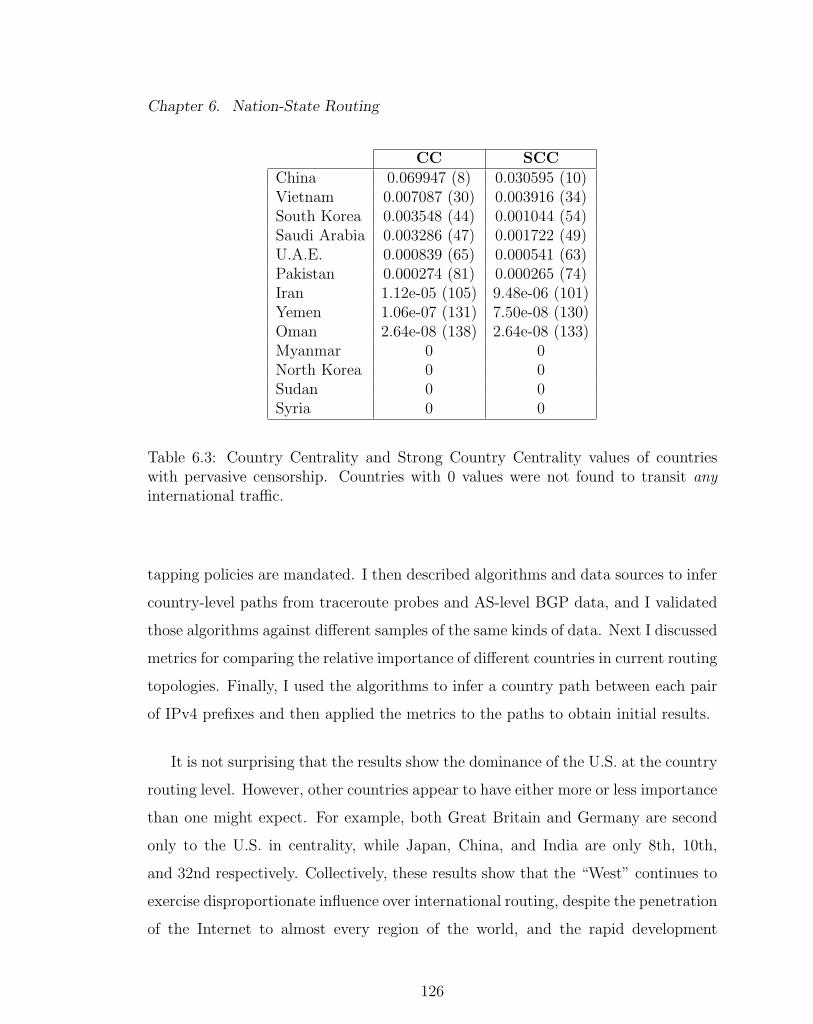
Chapter 6. Nation-State Routing
CC SCCChina 0.069947 (8) 0.030595 (10)Vietnam 0.007087 (30) 0.003916 (34)South Korea 0.003548 (44) 0.001044 (54)Saudi Arabia 0.003286 (47) 0.001722 (49)U.A.E. 0.000839 (65) 0.000541 (63)Pakistan 0.000274 (81) 0.000265 (74)Iran 1.12e-05 (105) 9.48e-06 (101)Yemen 1.06e-07 (131) 7.50e-08 (130)Oman 2.64e-08 (138) 2.64e-08 (133)Myanmar 0 0North Korea 0 0Sudan 0 0Syria 0 0
Table 6.3: Country Centrality and Strong Country Centrality values of countrieswith pervasive censorship. Countries with 0 values were not found to transit anyinternational traffic.
tapping policies are mandated. I then described algorithms and data sources to infer
country-level paths from traceroute probes and AS-level BGP data, and I validated
those algorithms against different samples of the same kinds of data. Next I discussed
metrics for comparing the relative importance of different countries in current routing
topologies. Finally, I used the algorithms to infer a country path between each pair
of IPv4 prefixes and then applied the metrics to the paths to obtain initial results.
It is not surprising that the results show the dominance of the U.S. at the country
routing level. However, other countries appear to have either more or less importance
than one might expect. For example, both Great Britain and Germany are second
only to the U.S. in centrality, while Japan, China, and India are only 8th, 10th,
and 32nd respectively. Collectively, these results show that the “West” continues to
exercise disproportionate influence over international routing, despite the penetration
of the Internet to almost every region of the world, and the rapid development
126

Chapter 6. Nation-State Routing
of China and India. Beyond what the results tell us about the Internet today, I
see the methods described in this dissertation as helping network designers, policy
makers, and researchers better understand the likely impact of national policies on
user privacy and the access to politically or socially sensitive content.
127

Chapter 7
Future Work and Conclusion
It is surprising that the Internet is so vulnerable to disruption, given its economic and
social importance. In part, this is because existing security proposals rely upon global
deployment before they can offer significant security gain. This dissertation measured
the Internet’s structure, modeled it, and exploited its redundant connectivity at the
AS-level to develop a distributed security solution for the BGP routing protocol.
After discussing future work in Section 7.1, I discuss the dissertation’s contributions
and conclude in Section 7.2.
7.1 Future Work
The work presented in this dissertation could be continued in many directions. First,
the soft-response mechanism introduced in Pretty Good BGP could be used to secure
other network protocols, such as DNS. DNS servers and clients do not ensure that
the IP addresses that they have for each domain name are legitimate. This might
allow a rogue DNS server to misdirect clients towards malicious destinations. For
instance, a bank’s website might be impersonated in order to steal user’s passwords.
128
Chapter 7. Future Work and Conclusion
The principle of trusting stable information, as found in PGBGP, could be applied
to DNS. Therefore, if a bank’s stable IP address is changed, it could be considered
an anomaly. And, as a soft response, both the trusted IP address and the anomalous
IP could be returned in a DNS response for twenty four hours. Clients could then
be configured to use the anomalous IP only if the trusted IP does not work.
The BGP security work could also be extended towards discovering optimal de-
ployment techniques. For instance, it would be useful to know what the minimal
necessary deployment of a security solution might be to protect routing or DNS. My
simulator, BSIM, could be used to help answer this question.
Next, many interesting extensions of ASIM are possible. For example, the model
could include business agreements between the different agents (similar to Ref. [116,
113]), or change the traffic patterns from person–to–person communication to a situ-
ation with more traffic originating from central servers. I could also model intra-AS
routing. Many of today’s ASes employ “hot-potato” routing and transfer packets
to the next AS as quickly as possible, to reduce cost. Alternative intra-AS routing
strategies, such as routing the packet as close to the destination as possible, could
be tested within the model’s framework.
Finally, my exploration of nation-state routing introduces many new opportuni-
ties for research. First, there are several potential sources of bias in the data sets I
used, which could potentially impact the results. It is believed that the Internet’s
topology is significantly larger than what can be observed in BGP RIBs [153]. For
example, peer-peer connections are only visible to customers of the peers (due to the
valley-free rule) and are thus difficult to find [154]. Fortunately, it is believed that
customer-provider edges are well represented in the observed RIBs. The topologies
that I extracted from the RIBs support these suppositions. As shown in 6.2.1, the
number of peer-peer edges increases by 90% between the testing set and the total
set while customer-provider edges only increased by 5%. Peer-peer edges typically
129

Chapter 7. Future Work and Conclusion
have less impact on routing than customer-provider edges, since only the down-
stream customers of the two peers can route through peer-peer edges. In addition,
I suspect that peer-peer edges, for the most part, arise between ASes in the same
country, or at least the same small geographic region (e.g., between two countries in
Europe), which would also limit their influence on the international flow of traffic
through the Internet. Still, the missing edges could have impact on the results of
my measurements. To test this, I plan to run the algorithms on multiple inferred
and generated [155, 86] topologies, including traceroute measurements collected from
larger number of vantage points [156].
Beyond the question of bias, I would also like to study the evolution of country
centrality over time. It has been suggested that the United States transits a smaller
fraction of total traffic than in the past. It would be interesting to know if the
United States has also become less central in terms of reachability, and if so why.
Which countries are becoming more central over time and which less so? It would
also be interesting to know how my results would change if I incorporated more
realistic models of interdomain traffic [157]. A more long-term question involves un-
derstanding the economically-driven strategies that single countries or small groups
of countries could adopt, either to enhance their own centrality or to reduce the
centrality of other countries (e.g., such as overlay routing). There may also be other
network measures that are of interest. Deletion impact or measures that incorporate
some component of traffic are two obvious directions.
Finally, it would be interesting to study the paths of domestic traffic. What frac-
tion of domestic paths (those that have a source and destination within the same
country) are actually routed through another country? Answering this question
would provide insight into the influence that foreign nations have over a country’s
domestic routing and security, and would shed light on a question posed in [130] con-
cerning whether warrantless wiretapping on links connecting one country to another
130

Chapter 7. Future Work and Conclusion
might inadvertently capture some purely domestic traffic. The framework developed
in this dissertation could be extended to address that question.
7.2 Concluding Remarks
This dissertation explored Internet security from a distributed perspective. First, it
introduced Pretty Good BGP (PGBGP). PGBGP is the first BGP security proposal
that could provide significant security to early adopters. It is an anomaly detector
coupled with a soft-response mechanism that has provable security guarantees. I
built a reference implementation of Pretty Good BGP, and it is currently used to
warn hundreds of network operators around the world of routing misconfigurations
and attacks.
Further, this dissertation explored the Internet’s structure at the AS-level. I
presented a new generative model of AS-like graphs, ASIM, which could be used to
test new network protocols. ASIM produces graphs statistically similar to the real
AS-graph both in degree distribution as well as from the radial perspective.
Finally, it was shown that Autonomous Systems sometimes act in unison, en-
forcing policies dictated by governments (such as censorship and wiretaps). This
dissertation introduced a framework for analyzing the Internet at the country level,
in order to better understand how much influence each country has over Internet
reachability.
131

References
[1] Renesys Blog, “Pakistan Hijacks YouTube.” http://www.renesys.com/blog/
2008/02/pakistan_hijacks_youtube_1.shtml.
[2] W. Blogs, “Revealed: The Internet’s biggest security hole.” http://blog.
wired.com/27bstroke6/2008/08/revealed-the-in.html.
[3] M. Roughan, S. J. Tuke, and O. Maennel, “Bigfoot, Sasquatch, the Yeti andother missing links: what we don’t know about the AS graph,” in SIGCOMMconference on Internet Measurement.
[4] A. B. Somayaji, Operating System Stability and Security through Process Home-ostasis. PhD thesis, University of New Mexico, July 2002.
[5] J. Balthrop, “RIOT: A responsive system for mitigating computer networkepidemics and attacks,” Master’s thesis, University of New Mexico, 2005.
[6] M. M. Williamson, “Throttling viruses: Restricting propagation to defeat ma-licious mobile code,” in Proc. ACSAC Security Conference, 2002.
[7] A.-L. Barabasi and R. Albert, “Emergence of scaling in random networks,”Science, vol. 286, pp. 509–512, October 1999.
[8] J. I. Alvarez-Hamelin and N. Schabanel, “An Internet graph model based ontrade-off optimization,” Eur. Phys. J. B, vol. 38, pp. 231–237, 2004.
[9] J. R. Crandall, D. Zinn, M. Byrd, E. Barr, and R. East, “ConceptDoppler: Aweather tracker for internet censorship,” 2007.
[10] R. J. Deibert, J. G. Palfrey, R. Rohozinski, and J. Zittrain, Access Denied:The Practice and Policy of Global Internet Filtering (Information Revolutionand Global Politics). MIT Press, 2008.
132
References
[11] Y. Rekhter, T. Li, and S. Hares, “A Border Gateway Protocol 4 (BGP-4).”RFC 4271, Jan. 2006.
[12] L. Gao and J. Rexford, “Stable Internet routing without global coordination,”IEEE/ACM Trans. on Networking, vol. 9, pp. 681–692, December 2001.
[13] M. Caesar and J. Rexford, “BGP policies in ISP networks,” IEEE NetworkMagazine, October 2005.
[14] L. Gao, “On inferring autonomous system relationships in the Internet,”IEEE/ACM Trans. on Networking, vol. 9, December 2001.
[15] K. Lougheed and Y. Rekhter, “Border Gateway Protocol (BGP).” RFC 1105(Experimental), June 1989. Made obsolete by RFC 1163.
[16] D. Mills, “Exterior Gateway Protocol formal specification.” RFC 904 (His-toric), Apr. 1984.
[17] K. Lougheed and Y. Rekhter, “Border Gateway Protocol (BGP).” RFC 1163(Historic), June 1990. Made obsolete by RFC 1267.
[18] K. Lougheed and Y. Rekhter, “Border Gateway Protocol 3 (BGP-3).” RFC1267 (Historic), Oct. 1991.
[19] Y. Rekhter and T. Li, “A Border Gateway Protocol 4 (BGP-4).” RFC 1654(Proposed Standard), July 1994. Made obsolete by RFC 1771.
[20] Y. Rekhter and T. Li, “A Border Gateway Protocol 4 (BGP-4).” RFC 1771(Draft Standard), Mar. 1995. Made obsolete by RFC 4271.
[21] Y. Rekhter, T. Li, and S. Hares, “A Border Gateway Protocol 4 (BGP-4).”RFC 4271 (Draft Standard), Jan. 2006.
[22] H. Ballani, P. Francis, and X. Zhang, “A study of prefix hijacking and inter-ception in the Internet,” in SIGCOMM, (New York, NY, USA), pp. 265–276,ACM, 2007.
[23] A. Ramachandran and N. Feamster, “Understanding the network-level behav-ior of spammers,” in Proc. ACM SIGCOMM, (New York, NY, USA), pp. 291–302, 2006.
[24] Internet Alert Registry forums. http://cs.unm.edu/~karlinjf/IAR/
phpBB2/viewtopic.php?t=30, Nov. 2006.
[25] Renesys Blog, “Con-Ed Steals the ’Net.” http://www.renesys.com/blog/
2006/01/coned_steals_the_net.shtml.
133

References
[26] C. Kruegel, D. Mutz, W. Robertson, and FredrikValeur, “Topology-based de-tection of anomalous BGP messages,” in Proc. Syposium on Recent Advancesin Intrusion Detection, vol. 2820, pp. 17–35, September 2003.
[27] American Registry for Internet Numbers. http://www.arin.net.
[28] RIPE. http://www.ripe.net/.
[29] Asia Pacific Network Information Centre. http://www.apnic.net.
[30] R. Mahajan, D. Wetherall, and T. Anderson, “Understanding BGP misconfig-uration,” in Proc. ACM SIGCOMM, pp. 3–16, 2002.
[31] W. Leibzon, “Question on 7.0.0.0/8.” http://www.merit.edu/mail.
archives/nanog/msg05883.html, Apr. 2007.
[32] X. Zhao, D. Pei, L. Wang, D. Massey, A. Mankin, S. F. Wu, and L. Zhang,“An analysis of BGP multiple origin AS (MOAS) conflicts,” in Proc. InternetMeasurement Workshop, Nov. 2001.
[33] X. Zhao, D. Pei, L. Wang, D. Massey, A. Mankin, S. F. Wu, and L. Zhang, “De-tection of invalid routing announcement in the Internet,” in Proc. DependableSystems and Networks, 2002.
[34] L. Subramanian, V. Roth, I. Stoica, S. Shenker, and R. Katz, “Listen andWhisper: Security mechanisms for BGP,” in Proc. Networked Systems Designand Implementation, March 2004.
[35] “RIPE whois registry.” http://www.ripe.net/whois.
[36] L. Wang, X. Zhao, D. Pei, R. Bush, D. Massey, and L. Zhang, “ProtectingBGP routes to top level DNS servers,” IEEE Transactions on Parallel andDistributed Systems, vol. 14, no. 9, pp. 851–860, 2003.
[37] J. Rexford, J. Wang, Z. Xiao, and Y. Zhang, “BGP routing stability of populardestinations,” in Proc. Internet Measurement Workshop, 2002.
[38] G. Goodell, W. Aiello, T. Griffin, J. Ioannidis, P. McDaniel, and A. Rubin,“Working around BGP: An incremental approach to improving security andaccuracy of interdomain routing,” in Proc. Network and Distributed SystemsSecurity, February 2003.
[39] S. Qui, F. Monrose, A. Terzis, and P. McDaniel, “Efficient techniques for de-tecting false origin advertisements in inter-domain routing,” Proceedings of TheSecond Workshop on Secure Network Protocols, Nov. 2006.
134

References
[40] “Renesys corporation.” http://www.renesys.com/.
[41] Renesys routing intelligence. http://www.renesys.com/products_services/routing_intelligence/.
[42] M. Lad, D. Massey, D. Pei, Y. Wu, B. Zhang, and L. Zhang, “PHAS: A prefixhijack alert system,” in Proc. USENIX Security Symposium, 2006.
[43] RIPE NCC MyASN service. http://www.ris.ripe.net/myasn.html.
[44] D. Moore, C. Shannon, G. Voelker, and S. Savage, “Internet quarantine: Re-quirements for containing self-propagating code,” in INFOCOM, pp. 285–294,April 2003.
[45] R. Perlman, “Network layer protocols with byzantine robustness,” 1988.
[46] B. R. Smith, S. Murthy, and J. J. Garcia-Luna-Aceves, “Securing distancevec-tor routing protocols,” 1997.
[47] B. Smith and J. Garcia-Luna-Aceves, “Securing the border gateway routingprotocol,” in Proc. Global Internet, November 1996.
[48] B. Kumar, “Integration of security in network routing protocols,” SIGSACRev., vol. 11, no. 2, pp. 18–25, 1993.
[49] S. Kent, C. Lynn, and K. Seo, “Secure border gateway protocol,” IEEE Journalon Selected Areas in Communications, vol. 18, no. 4, pp. 582–592, 2000.
[50] J. Ng, “Extensions to BGP to support secure origin BGP (soBGP),” expiredInternet Draft draft-ng-sobgp-bgp-extensions-02, April 2004.
[51] “Cisco systems incorporated.” http://www.cisco.com/.
[52] T. Wan, E. Kranakis, and P. van Oorschot, “Pretty secure BGP, psBGP,” inProc. Network and Distributed System Security, 2005.
[53] Y.-C. Hu, D. McGrew, A. Perrig, B. Weis, and D. Wendlandt, “(r)Evolutionarybootstrapping of a global PKI for securing BGP,” in Hot Topics in NetworksWorkshop, Nov. 2006.
[54] H. V. Madhyastha, T. Isdal, M. Piatek, C. Dixon, T. Anderson, A. Krishna-murthy, and A. Venkataramani, “iplane: An information plane for distributedservices,” OSDI, 2006.
135

References
[55] P. Mahadevan, D. Krioukov, M. Fomenkov, B. Huffaker, X. Dimitropoulos,k. claffy, and A. Vahdat, “Lessons from three views of the internet topology,”tech. rep., CAIDA Technical Report, 2005.
[56] RouteViews. http://www.routeviews.org/.
[57] RIPE RIS. http://www.ripe.net/projects/ris/.
[58] Z. M. Mao, L. Qiu, J. Wang, and Y. Zhang, “On AS-level path inference,” inSIGMETRICS, (New York, NY, USA), pp. 339–349, ACM, 2005.
[59] L. Gao, “On inferring autonomous system relationships in the Internet,”IEEE/ACM Trans. on Networking, vol. 9, December 2001.
[60] L. Subramanian, S. Agarwal, J. Rexford, and R. H. Katz, “Characterizing theinternet hierarchy from multiple vantage points,” in Proc. of IEEE INFOCOM2002, New York, NY, Jun 2002.
[61] G. D. Battista, M. Patrignani, and M. Pizzonia, “Computing the types of therelationships between autonomous systems,” in Proc. IEEE INFOCOM, 2003.
[62] T. Erlebach, A. Hall, and T. Schank, “Classifying customer-provider relation-ships in the internet,” Proceedings of the IASTED International Conference onCommunications and Computer Networks (CCN), 2002.
[63] X. Dimitropoulos and G. Riley, “Modeling autonomous-system relationships,”in PADS ’06: Proceedings of the 20th Workshop on Principles of Advanced andDistributed Simulation, (Washington, DC, USA), pp. 143–149, IEEE ComputerSociety, 2006.
[64] J. Qiu and L. Gao, “AS path inference by exploiting known AS paths,” inProceedings of IEEE GLOBECOM, 2005.
[65] W. Muhlbauer, A. Feldmann, O. Maennel, M. Roughan, and S. Uhlig, “Build-ing an AS-topology model that captures route diversity,” SIGCOMM, 2006.
[66] H. V. Madhyastha, T. Anderson, A. Krishnamurthy, N. Spring, andA. Venkataramani, “A structural approach to latency prediction,” IMC, 2006.
[67] M. Faloutsos, P. Faloutsos, and C. Faloutsos, “On power-law relationships ofthe Internet topology,” Comput. Commun. Rev., vol. 29, pp. 251–262, 1999.
[68] A. Fabrikant, E. Koutsoupias, and C. H. Papadimitriou, “Heuristically opti-mized trade-offs: A new paradigm for power laws in the Internet,” in Pro-ceedings of the 29th International Conference on Automata, Languages, and
136

References
Programming, vol. 2380 of Lecture notes in Computer science, (Heidelberg),pp. 110–122, Springer, 2002.
[69] J. I. Alvarez-Hamelin and N. Schabanel, “An internet graph model based ontrade-off optimization,” Eur. Phys. J. B, vol. 38, pp. 231–237, 2004.
[70] A. Medina, I. Matta, and J. Byers, “On the origin of power laws in Internettopologies,” ACM Computer Communication Review, vol. 30, pp. 18–28, 2000.
[71] J. Winick and S. Jamin, “Inet-3.0: Internet topology generator,” tech. rep.,University of Michigan CS Dept., 2000.
[72] H. Chan, D. Dash, A. Perrig, and H. Zhang, “Modeling adoptability of secureBGP protocol,” in SIGCOMM, (New York, NY, USA), pp. 279–290, ACM,2006.
[73] J. Karlin, S. Forrest, and J. Rexford, “Pretty good BGP: Improving BGPby cautiously adopting routes,” in Proc. IEEE International Conference onNetwork Protocols, Nov 2006.
[74] J. Karlin, S. Forrest, and J. Rexford, “Autonomous security for autonomoussystems,” Computer Networks Special Issue on Complex Computer and Com-munication Networks, vol. 52, no. 15, pp. 2908–2923, 2008.
[75] North American Network Operators Group. http://www.nanog.org.
[76] African Network Operators Group. http://www.afnog.org.
[77] Australian Network Operators Group. http://www.ausnog.net.
[78] Japan Network Operators Group. http://www.janog.gr.jp.
[79] Pacific Network Operators Group. http://www.pacnog.org.
[80] “The quagga software routing suite.”
[81] J. Karlin, S. Forrest, and J. Rexford, “BGP simulator (BSIM).” http://cs.
unm.edu/~karlinjf/pgbgp/.
[82] The CAIDA AS relationships dataset. http://www.caida.org/data/active/as-relationships/, Feb. 2007.
[83] X. Hu and Z. M. Mao, “Accurate real-time identification of IP prefix hijacking,”in Proceedings of IEEE Security and Privacy, 2007.
137

References
[84] C. Zheng, L. Ji, D. Pei, J. Wang, and P. Francis, “A light-weight distributedscheme for detecting ip prefix hijacks in real-time,” in Proc. ACM SIGCOMM,pp. 277–288, 2007.
[85] P. Holme, J. Karlin, and S. Forrest, “Radial structure of the Internet,” Pro-ceedings of the Royal Society A, vol. 463, pp. 1231–1246, 2007.
[86] P. Holme, J. Karlin, and S. Forrest, “An integrated model of traffic, geographyand economy in the internet,” ACM SIGCOMM CCR, 2008.
[87] A.-L. Albert, R & Barabasi, “Statistical mechanics of complex networks,” Rev.Mod. Phys, vol. 74, pp. 47–98, 2002.
[88] S. N. Dorogovtsev and J. F. F. Mendes, Evolution of Networks: From BiologicalNets to the Internet and WWW. Oxford University Press, Oxford, 2003.
[89] M. E. J. Newman, “The structure and function of complex networks,” SIAMReview, vol. 45, pp. 167–256, 2003.
[90] R. Pastor-Santorras and A. Vespignani, Evolution and structure of the Internet: a statistical physics approach. Cambridge: Cambridge Univeristy Press, 2004.
[91] J. C. Doyle, D. L. Alderson, L. Li, S. Low, M. Roughan, S. Shalunov,R. Tanaka, and W. Willinger, “The “ robust yet fragile” nature of the In-ternet,” Proc. Natl. Acad. Sci., vol. 102, pp. 14497–14502, 2005.
[92] A. Trusina, S. Maslov, P. Minnhagen, and K. Sneppen, “Hierarchy measuresin complex networks,” Phys. Rev. Lett., vol. 92, 2004.
[93] H. Chang, R. Govindan, S. Jamin, S. J. Shenker, and W. Willinger, “Towardscapturing representative as-level internet topologies,” tech. rep., University ofMichigan CS Dept., 2002.
[94] “Looking glass servers.” http://www.traceroute.org.
[95] D. Gale, “A theorem of flows in networks,” Pacific J. Math., vol. 7, pp. 1073–1082, 1957.
[96] J. M. Roberts Jr., “Simple methods for simulating sociomatrices with givenmarginal,” Social Networks, vol. 22, pp. 273–283, 2000.
[97] R. Pastor-Satorras, A. Vazquez, and A. Vespignani, “Dynamical and correla-tion properties of the Internet,” Phys. Rev. Lett., vol. 87, 2001.
[98] F. Buckley and F. Harary, Distance in graphs. Addison-Wesley, Redwood City,1989.
138

References
[99] G. Sabidussi, “The centrality index of a graph.,” Psychometrika, vol. 31,pp. 581–603, 1966.
[100] J. I. Alvarez-Hamelin, L. Dall’Asta, A. Barrat, and A. Vespignani, “Large scalenetworks fingerprinting and visualization using the k-core decomposition,” inAdvances in Neural Information Processing Systems, 2006.
[101] K. Nakao, “Distribution of measures of centrality: Enumerated distributionsof freeman’s graph centrality measures,” Connections, vol. 13, pp. 10–22, 1990.
[102] C.-Y. Lee, “Correlations among centrality measures in complex networks,” e-print physics/0605220, 2006.
[103] P. Holme, B. J. Kim, C. N. Yoon, and S. K. Han, “Attack vulnerability ofcomplex networks,” Phys. Rev. E, vol. 65, 2002.
[104] P. Mahadevan, D. Krioukov, M. Fomenkov, B. Huffaker, X. Dimitropoulos,K. C. Claffy, and A. Vahdat, “Lessons from three views of the Internet topol-ogy,” tech. rep., CAIDA tr-2005-02, 2005.
[105] S. Maslov, K. Sneppen, and A. Zaliznyak, “Detection of topological patternsin complex networks: Correlation profile of the Internet,” Physica A, vol. 333,2004.
[106] P. Mahadevan, D. Krioukov, M. Fomenkov, B. Huffaker, C. K. C. Dimitropou-los, X, and A. Vahdat, “The Internet AS-level topology: Three data sourcesand one definitive metric,” ACM SIGCOMM Computer Communications Re-view, vol. 36, pp. 17–26, 2006.
[107] R. Albert, H. Jeong, and A.-L. Barabasi, “Attack and error tolerance of com-plex networks,” Nature, vol. 406, pp. 378–382, 2000.
[108] D. J. Watts and S. H. Strogatz, “Collective dynamics of “small-world” net-works,” Nature, vol. 393, pp. 440–442, 1998.
[109] M. E. J. Newman, “Scientific collaboration networks. II. Shortest paths,weighted networks, and centrality,” Phys. Rev. E, vol. 64, 2001.
[110] E. Bonabeau, “Agent-based modeling: Methods and techniques for simulatinghuman systems,” Proc Natl Acad Sci, vol. 99, pp. 7280–7287, 2002.
[111] J. M. Carlson and J. Doyle, “Highly optimized tolerance: a mechanism forpower laws in designed systems,” Phys. Rev. E, vol. 60, pp. 1412–1427, August1999.
139

References
[112] H. Chang, S. Jamin, and W. Willinger, “Internet connectivity at the AS-level:an optimization-driven modeling approach,” in MoMeTools ’03: Proceedings ofthe ACM SIGCOMM workshop on Models, methods and tools for reproduciblenetwork research, (New York, NY, USA), pp. 33–46, ACM, 2003.
[113] H. Chang, S. Jamin, and W. Willinger, “To peer or not to peer: Modeling theevolution of the Internet’s AS-level topology,” in SIGCOMM, 2006.
[114] S. Bar, M. Gonena, and A. Wool, “A geographic directed preferential Internettopology model,” Computer Networks, vol. 51, pp. 4174–4188, 2007.
[115] L. Gao, “On inferring autonomous system relationships in the Internet,” IEEE/ ACM Transactions on Networking, vol. 9, pp. 733–745, 2001.
[116] S. Shakkottai, T. Vest, D. Krioukov, and K. C. Claffy, “Economic evolution ofthe Internet AS-level ecosystem.” e-print arxiv:cs.NI/0608058, 2006.
[117] I. Daubechies, K. Drakakis, and T. Khovanova, “A detailed study of the at-tachment strategies of new autonomous systems in the AS connectivity graph,”Internet Mathematics, vol. 2, pp. 185–246, 2006.
[118] P. Holme, “Congestion and centrality in traffic flow on complex networks,”Advances in Complex Systems, vol. 6, pp. 163–176, 2003.
[119] P. Echenique, J. Gomez-Gardenes, and Y. Moreno, “Dynamics of jammingtransitions in complex networks,” Europhys. Lett., vol. 71, pp. 325–331, 2005.
[120] V. Sood and P. Grassberger, “Localization transition of biased random walkson random networks,” Phys. Rev. Lett., vol. 99, p. 098701, 2007.
[121] L. Gao and F. Wang, “The extent of AS path inflation by routing policies,” inProceedings of GLOBECOM ’02, vol. 3, pp. 2180–2184, 2002.
[122] F. Cairncross, The death of distance. Boston, MA: Harvard Business SchoolPress, 1997.
[123] W. Isard, Location and space economy. Cambridge MA: MIT Press, 1956.
[124] R. Cohen, K. Erez, D. ben Avraham, and S. Havlin, “Resilience of the Internetto random breakdowns,” Phys. Rev. Lett., vol. 85, pp. 4626–4628, 2000.
[125] S.-H. Yook, H. Jeong, and A.-L. Barabasi, “Modeling the Internet’s large-scaletopology,” Proc. Natl. Acad. Sci. USA, vol. 99, pp. 13382–13386, 2002.
[126] P. L. Krapivsky, S. Redner, and F. Leyvraz, “Connectivity of growing randomnetworks,” Phys. Rev. Lett., vol. 85, pp. 4629 – 4632, 2000.
140

References
[127] K.-I. Goh, E. Oh, H. Jeong, B. Kahng, and D. Kim, “Classification of scale-freenetworks,” Proc. Natl. Acad. Sci. USA, vol. 99, pp. 12583–12588, 2002.
[128] N. Spring, R. Mahajan, D. Wetherall, and T. Anderson, “Measuring ISPtopologies with Rocketfuel,” IEEE / ACM Transactions of Networking, vol. 12,pp. 2–16, 2004.
[129] A. Lakhina, J. W. Byers, M. Crovella, and I. Matta, “On the geographic loca-tion of Internet resources,” Tech. Rep. BUCS-TR-2002-015, Boston University,2002.
[130] S. M. Bellovin, M. Blaze, W. Diffie, S. Landau, P. G. Neumann, and J. Rexford,“Risking communications security: Potential hazards of the Protect AmericaAct,” IEEE Security and Privacy, 2008.
[131] “Securing the federal government’s domain name system infrastructure.” http://www.whitehouse.gov/omb/memoranda/fy2008/m08-23.pdf, 2008.
[132] “Transition planning for Internet protocol version 6 (IPv6).” http:
//georgewbush-whitehouse.archives.gov/omb/memoranda/fy2005/
m05-22.pdf, 2005.
[133] R. Clayton, “Anonymity and traceability in cyberspace,” Tech. Rep. UCAM-CL-TR-653, University of Cambridge, 2005.
[134] YouTube. http://www.youtube.com/.
[135] X. Wang, S. Chen, and S. Jajodia, “Tracking anonymous peer-to-peer VoIPcalls on the Internet,” in ACM Conference on Computer and CommunicationsSecurity, 2005.
[136] D. Andersen, H. Balakrishnan, F. Kaashoek, and R. Morris, “Resilient overlaynetworks,” in ACM Symposium on Operating Systems Principles, pp. 131–145,2001.
[137] A. Broido and kc claffy, “Analysis of RouteViews BGP data: Policy atoms,”in Proceedings of the NRDSM workshop, 2001.
[138] A. Broido and K. Claffy, “Complexity of global routing policies,” in IMA, 2001.
[139] U. of Oregon, “Routeviews project.” http://www.routeviews.org, 2005.
[140] K. Sriram, O. Borchert, O. Kim, P. Gleichmann, and D. Montgomery, “Acomparative analysis of BGP anomaly detection and robustness algorithms,”to appear in the Proceedings of CATCH, 2009.
141

References
[141] B. Chun, D. Culler, T. Roscoe, A. Bavier, L. Peterson, M. Wawrzoniak, andM. Bowman, “Planetlab: An overlay testbed for broad-coverage services,” inSIGCOMM, 2003.
[142] “Team Cymru.” http://www.cymru.com/.
[143] N. Spring, R. Mahajan, D. Wetherall, and T. Anderson, “Measuring ISPtopologies with Rocketfuel,” IEEE/ACM Transactions on Networking, 2004.
[144] “Sarangworld project.” http://www.sarangworld.com/TRACEROUTE/.
[145] J. Moy, “OSPF version 2.” RFC 2328, 1998.
[146] R. Callon, “Use of OSI IS-IS for routing in TCP/IP and dual environments.”RFC 1195, 1990.
[147] L. Freeman, “A set of measures of centrality based on betweenness,” Sociom-etry, vol. 40, pp. 35–41, 1977.
[148] L. C. Freeman, “Centrality in social networks: Conceptual clarification,” SocialNetworks, vol. 1, no. 3, pp. 215–239, 1979.
[149] G. Sabidussi, “The centrality index of a graph,” Psychometrika, vol. 31,pp. 581–603, 1966.
[150] P. Mahadevan, D. Krioukov, M. Fomenkov, X. Dimitropoulos, Claffy, andA. Vahdat, “The Internet AS-level topology: Three data sources and one defini-tive metric,” SIGCOMM Comput. Commun. Rev., vol. 36, no. 1, pp. 17–26,2006.
[151] S. Zhou and R. J. Mondragon, “Accurately modeling the Internet topology,”Phys. Rev. E, vol. 70, p. 066108, Dec 2004.
[152] “Opennet initiative.” http://opennet.net.
[153] R. V. Oliveira, D. Pei, W. Willinger, B. Zhang, and L. Zhang, “In searchof the elusive ground truth: the internet’s AS-level connectivity structure,”SIGMETRICS Perform. Eval. Rev., vol. 36, no. 1, pp. 217–228, 2008.
[154] H. Chang, R. Govindan, S. Jamin, S. J. Shenker, and W. Willinger, “Towardscapturing representative AS-level internet topologies,” in Computer NetworksJournal, pp. 737–755, 2004.
[155] H. Chang and S. Jamin, “To peer or not to peer: Modeling the evolution ofthe internet’s as-level topology,” In INFOCOM, 2006.
142
References
[156] The DIMES Project. http://www.netdimes.org.
[157] A. Feldmann, N. Kammenhuber, O. Maennel, B. Maggs, R. D. Prisco, andR. Sundaram, “A methodology for estimating interdomain web traffic de-mand,” in Internet Measurement Conference, pp. 322–335, 2004.
143