dissipation of the energy imparted by mid-latitude storms...

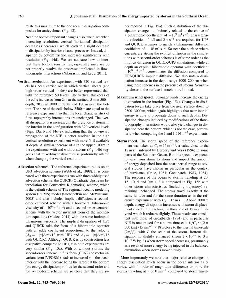
Ocean Sci., 12, 743–769, 2016www.ocean-sci.net/12/743/2016/doi:10.5194/os-12-743-2016© Author(s) 2016. CC Attribution 3.0 License.

Dissipation of the energy imparted by mid-latitude storms in theSouthern OceanJulien Jouanno1,2, Xavier Capet2, Gurvan Madec2,3, Guillaume Roullet4, and Patrice Klein4

1LEGOS, Université de Toulouse, IRD, CNRS, CNES, UPS, Toulouse, France2CNRS-IRD-Sorbonne Universités, UPMC, MNHN, LOCEAN Laboratory, Paris, France3National Oceanographic Centre, Southampton, UK4University of Brest, CNRS, IRD, Ifremer, Laboratoire d’Océanographie Physique et Spatiale (LOPS), IUEM, Brest, France

Correspondence to: Julien Jouanno ([email protected])

Received: 13 January 2016 – Published in Ocean Sci. Discuss.: 20 January 2016Revised: 14 April 2016 – Accepted: 25 April 2016 – Published: 1 June 2016

Abstract. The aim of this study is to clarify the role ofthe Southern Ocean storms on interior mixing and merid-ional overturning circulation. A periodic and idealized nu-merical model has been designed to represent the key phys-ical processes of a zonal portion of the Southern Ocean lo-cated between 70 and 40◦ S. It incorporates physical ingredi-ents deemed essential for Southern Ocean functioning: roughtopography, seasonally varying air–sea fluxes, and high-latitude storms with analytical form. The forcing strategy en-sures that the time mean wind stress is the same between thedifferent simulations, so the effect of the storms on the meanwind stress and resulting impacts on the Southern Ocean dy-namics are not considered in this study. Level and distribu-tion of mixing attributable to high-frequency winds are quan-tified and compared to those generated by eddy–topographyinteractions and dissipation of the balanced flow. Resultssuggest that (1) the synoptic atmospheric variability alonecan generate the levels of mid-depth dissipation frequentlyobserved in the Southern Ocean (10−10–10−9 W kg−1) and(2) the storms strengthen the overturning, primarily throughenhanced mixing in the upper 300 m, whereas deeper mixinghas a minor effect. The sensitivity of the results to horizontalresolution (20, 5, 2 and 1 km), vertical resolution and numer-ical choices is evaluated. Challenging issues concerning hownumerical models are able to represent interior mixing forcedby high-frequency winds are exposed and discussed, partic-ularly in the context of the overturning circulation. Overall,submesoscale-permitting ocean modeling exhibits importantdelicacies owing to a lack of convergence of key componentsof its energetics even when reaching 1x = 1 km.

1 Introduction

Knowledge gaps pertaining to energy dissipation and mixingdistribution in the ocean greatly limit our ability to apprehendits dynamical and biogeochemical functioning (globally or atsmaller scale, e.g., regional) and its role in the climate sys-tem evolution (Naveira-Garabato, 2012). For example, themeridional overturning circulation in low-resolution globalcoupled models is significantly altered by the parameteriza-tion for and intensity of vertical mixing (Jayne, 2009; Meletet al., 2013).

A great deal of effort is currently deployed to address theissue but the difficulties are immense: dissipation occurs in-termittently, heterogeneously and in relation to a myriad ofprocesses, whose importance varies depending on the region,depth range, season, proximity to bathymetric features, etc.In this context, establishing an observational truth based onlocal estimates involves probing the ocean at centimeter scale(vertically) with horizontal- and temporal-resolution require-ments that will need a long time to be met (e.g., MacKinnonet al., 2009 or DIMES program, Gille et al., 2012).

In order to make progress other (non-exclusive) ap-proaches are being followed. Well-constrained bulk-mixingrequirements for certain water masses can be exploited toinfer mixing rates and, in some cases point to (or discard)specific processes (de Lavergne et al., 2016). Alternatively,in-depth investigations of dissipation and mixing associatedwith presumably important processes are carried out (withthe subsequent parameterization of the effects in OGCMs(ocean general circulation models) being the ultimate objec-tive, Jayne, 2009; Jochum et al., 2013). This study belongs to

Published by Copernicus Publications on behalf of the European Geosciences Union.

744 J. Jouanno et al.: Dissipation of the energy imparted by storms in the Southern Ocean

the latter thread. It is a numerical contribution to the investi-gation of dissipation and mixing due to atmospheric synopticvariability (mid-latitude storms) in the Southern Ocean.

Synoptic or high-frequency winds inject importantamounts of energy into the ocean that feed the near-inertialwave (NIW) field. A large part of the near-inertial en-ergy (NIE) dissipates locally in the upper ocean, where itdeepens the mixed-layer and potentially has an impact onthe air–sea exchanges and global atmospheric circulation(Jochum et al., 2013). Nevertheless a substantial fraction ofthe NIE also spreads horizontally and vertically away fromits source regions: beta dispersion propagates the energy to-ward lower latitudes (Anderson and Gill, 1979), advection bythe geostrophic circulation redistributes NIE laterally (Zhaiet al., 2005) and the mesoscale eddy field favors the penetra-tion of NIWs into the deep ocean by shortening their horizon-tal scales (Danioux et al., 2008; Zhai et al., 2005), or throughthe “inertial chimney” effect (Kunze, 1985).

Although the near-inertial part of the internal wave spec-trum is thought to contain most of the energy and verti-cal shear (Garrett, 2001), large uncertainties remain on theamount of NIE available at depth for small-scale mixing andwhether/where it is significant compared to other sources ofmixing such as the breaking of internal waves generated bytides or the interaction of the mesoscale flow with rough to-pography (e.g., Nikurashin et al., 2013). The only presentconsensus is that NIE due to atmospheric forcing does notpenetrate efficiently enough into the ocean interior to pro-vide the mixing necessary to close the deep cells of the MOC(Meridional Overturning Circulation)(Furuichi et al., 2008;Ledwell et al., 2011), below 2000 m.

On the other hand, the vertical flux of NIE at 800 m esti-mated by Alford et al. (2012) at station Papa (in a part of thenorth Pacific not particularly affected by storm activity) mayhave significant implications on mixing of the interior watermasses, depending on the (unknown) depth range where itdissipates. Our regional focus is the Southern Ocean, whereintense storm activity forces NIW (Alford, 2003) that seemto have important consequences, at least above 1500 m depth.Elevated turbulence in the upper 1000–1500 m north of Ker-guelen plateau has been related to wind-forced downward-propagating near-inertial waves (Waterman et al., 2013); theclear seasonal cycle of diapycnal mixing estimated from over5000 ARGO profiles in regions of the Southern Ocean wheretopography is smooth points to the role of wind input in thenear-inertial range (and NIW penetration into the ocean inte-rior; Wu et al., 2011).

The aim of this study is to (i) further clarify the mecha-nisms implicated in NIW penetration into the ocean interior,(ii) more precisely quantify the resulting NIE dissipation in-tensity including its vertical distribution and (iii) better un-derstand the current (and future) OGCM limitations in repre-senting NIE dissipation. (Findings on ii will be specific to theSouthern Ocean while we expect those on i and iii to be moregeneric.) For that purpose, we perform semi-idealized South-

ern Ocean simulations for a wide range of model parame-ters and different numerical schemes covering eddy presentto submesoscale-rich regimes.

Importantly, our highest resolution simulations adequatelyresolve the meso- and submesoscale turbulent activitydeemed essential in the leakage of NIE out of the surfacelayers, as found in Danioux et al. (2011). In contrast to thisand other studies (Danioux et al., 2008), the realism of theocean forcing, mean state and circulation makes it more di-rectly applicable to the real ocean, provided that numericalrobustness and convergence is reasonably achieved.

The paper is organized as follows. The model setup is pre-sented in Sect. 2 and the ocean dynamics and mean state thatare simulated without storms are described in Sect. 3. Sec-tion 4 describes the spatial and temporal characteristics andconsequences of the simplified NIW field generated by thepassage of a single storm (spin-down experiment). In Sect. 5quasi-equilibrated simulations are analyzed in terms of path-ways through which the storm energy is deposited into theinterior ocean and sensitivity of the mixing distribution tostorm parameters and numerical choices. In Sect. 6, we char-acterize the long-term impact of the storms on the (large-scale) MOC, which turns out to be significant, mainly be-cause of their effect on and immediately below the oceansurface boundary layer. Section 7 provides some discussionand Sect. 8 concludes.

2 Model

The numerical setup consists of a periodic channel configu-ration 2000 km long (Lx , zonal direction) and 3000 km wide(Ly , meridional direction) that aims to represent a zonal por-tion of the Southern Ocean located between 70 and 40◦ S(Fig. 1). It is inspired by the experiment described in Aber-nathey et al. (2011), which is mainly adiabatic in the inte-rior. We add three ingredients to our reference experimentdeemed essential to reach realistic levels of dissipation andwhose consequence is to enhance dissipation and mixing inthe model ocean interior.

i. The bathymetry is random and rough. Horizontal scalesof the reference bathymetry range between 10 and100 km and depths vary between 3000 and 4000 m. Thebottom roughness, computed as the variance of the bot-tom height (H), is 3× 104 m2, which can be consideredas intermediate between rough and smooth and is rep-resentative of the roughness of a large portion of theSouthern Ocean topography (see map of roughness inWu et al., 2011). The inclusion of bottom topographyaims to limit the ACC transport through bottom formstress (Rintoul et al., 2001) and to generate deep andmid-depth mixing through vertical shear. Our horizon-tal resolution≥ 1 km and the hydrostatic approximationused to derive the model primitive equations do not per-mit the proper representation of upward radiation and

Ocean Sci., 12, 743–769, 2016 www.ocean-sci.net/12/743/2016/

J. Jouanno et al.: Dissipation of the energy imparted by storms in the Southern Ocean 745

2000 km 3000 km

4 km

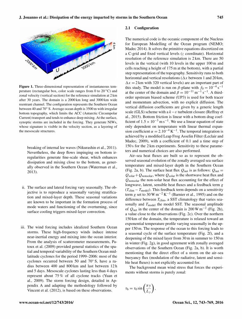
Figure 1. Three-dimensional representation of instantaneous tem-perature (rectangular box, color scale ranges from 0 to 20 ◦C) andzonal velocity (vertical section) for the reference simulation at 2 kmafter 30 years. The domain is a 2000 km long and 3000 km widereentrant channel. The configuration represents the Southern Oceanbetween 40 and 70◦ S. Average ocean depth is 3500 m with irregularbottom topography, which limits the ACC (Antarctic CircumpolarCurrent) transport and tends to enhance deep mixing. At the surface,synoptic storms are included in the forcing. They generate NIWs,whose signature is visible in the velocity section, as a layering ofthe mesoscale structures.

breaking of internal lee waves (Nikurashin et al., 2011).Nevertheless, the deep flows impinging on bottom ir-regularities generate fine-scale shear, which enhancesdissipation and mixing close to the bottom, as gener-ally observed in the Southern Ocean (Waterman et al.,2013).

ii. The surface and lateral forcing vary seasonally. The ob-jective is to reproduce a seasonally varying stratifica-tion and mixed-layer depth. These seasonal variationsare known to be important in the formation process ofmode waters and functioning of the overturning, sincesurface cooling triggers mixed-layer convection.

iii. The wind forcing includes idealized Southern Oceanstorms. These high-frequency winds induce intensenear-inertial energy and mixing into the ocean interior.From the analysis of scatterometer measurements, Pa-toux et al. (2009) provided general statistics of the spa-tial and temporal variability of the Southern Ocean mid-latitude cyclones for the period 1999–2006: most of thecyclones occurred between 50 and 70◦ S, have a ra-dius between 400 and 800 km and last between 12 hand 5 days. Mesoscale cyclones lasting less than 4 daysrepresent about 75 % of all cyclone tracks (Yuan etal., 2009). The storm forcing design, detailed in Ap-pendix A and adapting the methodology followed byVincent et al. (2012), is based on these observations.

2.1 Configuration

The numerical code is the oceanic component of the Nucleusfor European Modelling of the Ocean program (NEMO;Madec 2014). It solves the primitive equations discretized ona C-grid and fixed vertical levels (z coordinate). Horizontalresolution of the reference simulation is 2 km. There are 50levels in the vertical (with 10 levels in the upper 100 m andcells reaching a height of 175 m at the bottom), with a partialstep representation of the topography. Sensitivity runs to bothhorizontal and vertical resolutions (1x between 1 and 20 km,1x = 2 km with 320 vertical levels) are an important part ofthis study. The model is run on β-plane with f0 = 10−4 s−1

at the center of the domain and β = 10−11 m−1 s−1. A third-order upstream biased scheme (UP3) is used for both tracerand momentum advection, with no explicit diffusion. Thevertical diffusion coefficients are given by a generic lengthscale (GLS) scheme with a k−ε turbulent closure (Reffray etal., 2015). Bottom friction is linear with a bottom drag coef-ficient of 1.5× 10−3 m s−1. We use a linear equation of stateonly dependent on temperature with linear thermal expan-sion coefficient α = 2.10−4 K−1. The temporal integration isachieved by a modified Leap Frog Asselin Filter (Leclair andMadec, 2009), with a coefficient of 0.1 and a time step of150 s for the 2 km experiments. Sensitivity to these parame-ters and numerical choices are also performed.

Air–sea heat fluxes are built so as to represent the ob-served seasonal evolution of the zonally averaged sea surfacetemperature and mixed-layer depth in the Southern Ocean(Fig. 2a, b). The surface heat flux Qnet is as follows: Qnet =

Qsolar+Qnonsolar, whereQsolar is the shortwave heat flux andQnonsolar the non-solar heat flux accounting for the effect oflongwave, latent, sensible heat fluxes and a feedback term g

(Tclim−Tmodel). This feedback term depends on a sensitivityterm g set to 30 W m−2 K−1 (Barnier et al., 1995) and on thedifference between Tclim, a SST climatology that varies sea-sonally and Tmodel the model SST. The seasonal amplitudeof Qnet in the center of the domain is 200 W m−2 (Fig. 2h),a value close to the observations (Fig. 2c). Over the northern150 km of the domain, the temperature is relaxed toward anexponential temperature profile varying seasonally in the up-per 150 m. The response of the ocean to this forcing leads toa seasonal cycle of the surface temperature (Fig. 2f), and adeepening of the mixed layer from 30 m in summer to 150 min winter (Fig. 2g), in good agreement with zonally averagedobservations of the Southern Ocean (Fig. 2a, b). It is worthmentioning that the direct effect of a storm on the air–seabuoyancy flux (modulation of the radiative, latent and sensi-ble heat fluxes) is not explicitly accounted for.

The background mean wind stress that forces the experi-ments without storms is purely zonal:

τb = τ0 sin(πy

Ly

),

www.ocean-sci.net/12/743/2016/ Ocean Sci., 12, 743–769, 2016


Figure 2. Seasonal cycle of zonally averaged SST (a, f, ◦C), mixed-layer depth (b, g, m) computed in both model and observations with afixed threshold criterion of 0.2 ◦C relative to the temperature at 10 m, net air–sea heat flux (c, h, W m−2), and the solar (d, i, W m−2) andnon-solar (e, j, W m−2) components of the air–sea heat flux. Climatological seasonal cycles are built from observations (left column) andmodel outputs and forcing. Observations include OAFlux products (Yu et al., 2007) for the period 1984–2007 and de Boyer Montégut (2004)mixed-layer depth climatology. Model data are from the last 10 years of the 2 km reference simulation without storms.

where τ0 = 0.15 N m−2. In order to have exactly the same 10-year-mean wind stress between experiments with and with-out storms, the averaged residual wind due to the storm pas-sages is removed from τb in the experiment with storms.

Two long reference experiments, one with storms and an-other without storms, with a horizontal resolution of 2 kmhave been run for 40 years. For these experiments, the modelis started from a similar simulation without storms, equili-brated with a 200-year long spin-up at 5 km horizontal res-olution. Unless otherwise stated, the last 10 years of thesimulations are used for diagnostics, excluding the northern150 km band where restoring is applied. Similar long-termsimulations with a horizontal resolution of 20 and 5 km havealso been performed in order to determine meridional over-turning modifications with horizontal resolution (Sect. 7).

An experiment with a single storm traveling eastwardthrough the center of the basin over an equilibrated oceanhas also been performed. Initial conditions are taken fromthe 2 km horizontal resolution simulation (without storm) at(day) 31 December of year 30 from the 2 km reference exper-iment without storms. The storm is centered at the meridionalposition Ly/2 and has a maximum wind stress of 1.5 N m−2.The ocean spin-down response is analyzed for a period of 70days (the storm is centered at days 5, starting at day 3 andending at day 7).

In order to assess the sensitivity of interior mixing tonumerics and storms characteristics, additional experimentshave been run over shorter periods of 3 years, starting fromyear 30 of the 2 km reference experiment without storms.These experiments are summarized in Table 1 and will beanalyzed in Sect. 5. The last 2 years of these experimentsare used for diagnostics. Although the model is not equili-brated after a period of 3 years, we have verified in Sect. 5that changes in terms of energy dissipation and mixing diag-nosed over this short period are significant.

The averaged total wind work in the 2 km experiment withstorms is 16.8 mW m−2. This value is comparable to the20 mW m−2 input rates for the Southern Ocean estimatedby Wunsch (1998). The contribution from the near-inertialband is computed from instantaneous 2-hourly model out-puts, time filtered in the band {0.9,1.15}f following Al-ford et al. (2012). Near-inertial wind work is 1.4 mW m−2

for the entire domain and 2.2 mW m−2 in its central part(1000 km < y < 2000 km). These values are in agreement withSouthern Ocean estimates from drifters (Elipot and Gilles,2009;∼ 2 mW m−2), ocean general circulation models (Rathet al., 2014;∼ 1 mW m−2) and slab mixed-layer models (Al-ford, 2003; 1–2 mW m−2).



Table 1. Summary of numerical experiments.

Name 1x Nb vert. Dt Horiz. adv Storms Storm speed Tmaxlevels (Asselin coefficient) scheme (m s−1) (N m−2)

Sensitivity to horizontal and vertical resolution

20 km nostorm 20 km 50 1200 s (0.1) UP3 no20 km storms 20 km ” 1200 s (0.1) ” yes 15 1.55 km nostorm 5 km ” 300 s (0.1) ” no5 km storms 5 km ” 300 s (0.1) ” yes ” ”2 km nostorm 2 km ” 150 s (0.1) ” no2 km storms 2 km ” 150 s (0.1) ” yes ” ”1 km nostorm 1 km ” 60 s (0.1) ” no1 km storms 1 km ” 60 s (0.1) ” yes ” ”2 km nostorm_Z320 2 km 320 50 s (0.1) ” no2 km storms_Z320 ” 320 50 s (0.1) ” yes ” ”

Sensitivity to horizontal advection scheme

2 km nostorm_QUICK ” 50 150 s (0.1) QUICK no2 km storms_QUICK ” ” 150 s (0.1) QUICK yes ” ”2 km nostorm_CEN2 ” ” 100 s (0.1) CEN2 no2 km storms_CEN2 ” ” 100 s (0.1) CEN2 yes ” ”2 km nostorm_VFORM ” ” 100 s (0.1) VFORM no2 km storms_VFORM ” ” 100 s (0.1) VFORM yes ” ”

Sensitivity to storm characteristics

2 km storms_C0 ” ” 150 s (0.1) UP3 yes 0 ”2 km storms_C5 ” ” ” ” yes 5 ”2 km storms_C10 ” ” ” ” yes 10 ”2 km storms_C15 ” ” ” ” yes 15 ”2 km storms_C20 ” ” ” ” yes 20 ”2 km storms_TAU-1 ” ” ” ” yes 15 12 km storms_TAU-1.5 ” ” ” ” yes 15 1.52 km storms_TAU-3 ” ” ” ” yes 15 3

One storm experiments

2 km onestorm_A ” ” 150 s (0.1) ” yes 15 1.52 km onestorm_B ” ” 30 s (0.1) ” yes 15 1.52 km onestorm_C ” ” 150 s (0.01) ” yes 15 1.5

2.2 Energy diagnostics

Energy diagnostics and precise evaluations of the energy dis-sipation in the model are essential elements of our study.They are detailed below. The model kinetic energy (KE)equation can be written as follows:

12ρ0 ∂t u

2h︸︷︷︸

KE

=−ρ0 uh (uh · ∇h)uh− ρ0 uh ·w∂zuh︸︷︷︸ADV

(1)

− uh · ∇hp︸︷︷︸PRES

+ ρ0 uh ·Dh︸︷︷︸εh

+ ρ0 uh · ∇z (κv∇huh)︸︷︷︸εv

+Dtime,

where the subscript “h” denotes a horizontal vector, κv is thevertical viscosity,Dh the contribution of lateral diffusion pro-cesses andDtime the dissipation of kinetic energy by the timestepping scheme, which can be easily estimated in our sim-ulations since it only results from the application of the As-selin time filter. The dissipation of kinetic energy by spatialdiffusive processes is computed as the spatial integral of thediffusive terms εv and εh in Eq. (1):

Ev =

∫ ∫ ∫ρ0 uh · ∇z (κv∇zuh)︸︷︷︸

εv

dxdydz (2)

=

∫ ∫ ∫ (ρ0κv

∂uh

∂z·∂uh

∂z

)dxdydz

+

∫ ∫(uh · τs− uh · τb)dxdy,



Figure 3. Surface vorticity snapshot (s−1) over the entire modeldomain at (day) 31 December of year 39 from the 2 km horizontalresolution experiment without storms.

Eh =

∫ ∫ ∫ρ0 uh ·Dh︸︷︷︸

εv

dxdydz. (3)

As mentioned before, we do not specify explicit horizon-tal diffusion since it is implicitly treated by the UP3 advec-tion scheme we use (see numerical details in Madec, 2014).So the term Dh is evaluated at each time step as the dif-ference between horizontal advection momentum tendencycomputed with UP3 and the advection tendency given by anon-diffusive centered scheme alternative to UP3. Two op-tions are the second-order and fourth-order schemes imple-mented in NEMO. The second-order scheme is non-diffusivebut dispersive. The fourth-order scheme in NEMO involvesa fourth-order interpolation for the evaluation of advectivefluxes but their divergence is kept at second order, makingthe scheme not strictly non-diffusive. Although the estima-tion of UP3 horizontal diffusion depends on the scheme usedas a reference, we verify in Sect. 5 that the sensitivity ofdomain-averaged εh to the choice of the second- or fourth-order scheme is much smaller than that resulting from otherparameter changes, e.g., small changes in the characteristicsof the atmospheric forcing.

3 Ocean dynamics under low-frequency forcing

We first examine the dynamics and mean state of the experi-ment with a horizontal resolution of 2 km and without stormsin order to review the background oceanic conditions withinour zonal jet configuration. A snapshot of the surface vortic-ity field (Fig. 3) illustrates the broad range of scale resolvedby the 2 km model and the ubiquitous presence of meso- andsubmesoscale motions, including eddies and filaments. Theslope of the annual mean surface velocity spectrum in themeso- and submesoscale range is between k−2 and k−3. Thespectral slope varies seasonally (Fig. 4b), more noticeablyin the submesoscale range (60 km > λ; i.e., horizontal scalesbelow 10 km), between k−3 during summer and k−2 duringwinter (for the meso- and submesoscale range in Fig. 4b,the thin dark red line is superimposed on the thick dark redline). We interpret the increase of submesoscale energy dur-ing winter as a direct consequence of enhanced mixed-layerinstabilities in response to a deep mixed layer (Fox-Kemper,2008; Sasaki et al., 2014).

The energy contained at large scale and mesoscale (k <5× 10−5 rad m−1) decreases with depth as indicated by thespectra at 1000 and 2500 m (Fig. 4a). But note that the en-ergy contained in the wavenumber range 5×10−5 < k < 6×10−4 rad m−1 (i.e., the range associated with small mesoscalebordering with the submesoscale) is larger at 2500 m com-pared to 1000 m. This is due to an injection of energy atthese scales by the rough topography. As shown by instanta-neous velocity sections in Fig. 5a and b, the horizontal scalesof u and v below 2500 m are much shorter than the typicalscale of the upper-ocean mesoscale field. They correspondto the scale of the bathymetry, and are responsible for in-creased horizontal shear in the deep ocean (Fig. 5e), therebycontributing to the dissipation of the energy imparted by thewinds to the mean flow.

Vertical velocity rms is below 10 m day−1 over most of thewater column except near the bottom (i.e., below 2500 m)where it increases substantially to ∼ 100 m day−1 (Figs. 5cand 6b). Although flat bottom numerical solutions can alsoexhibit similar increases (Danioux et al., 2008), the spa-tiotemporal scales of w near the bottom (e.g., see Fig. 5c)suggest the importance of flow–topography interactions.

The average zonal transport in the reference experiment is∼ 300 Sv. Although the rough bathymetry strongly reducesthe transport compared to simulations with flat bottom (thatreach∼ 1000 Sv, not shown), the absence of any topographicridge and narrow passages does not allow us to obtain thetypical transport of∼ 130–150 Sv observed in the ACC (e.g.,Cunningham et al., 2003). As discussed in Abernathey etal. (2011), much of this elevated transport can be seen asa translation of the system westward that is not expectedto affect our investigation of fine-scale dynamics and its ef-fect on the transverse overturning circulation. The averageeddy kinetic energy (EKE) exceeds 0.05 m2 s−2 at the sur-



Figure 4. Horizontal velocity variance in the 2 km reference experiments with and without storms. (a) Kinetic energy power spectra asa function of wavenumber (rad m−1) at 0, 1000 and 2500 m depth. (b) Seasonal (summer is defined as December–January–February andwinter as June–July–August) kinetic energy power spectra at 0 and 1000 m depth. Spectra are built using instantaneous velocity taken each 5days of the last 2 years of the 2 km simulations. Kinetic energy contained in the wavelength ranges λ < 60 km (c), 60 km< λ < 600 km (d)and λ > 600 km (e) as a function of depth. In (b) and for wavenumber above 5× 10−5 rad m−1, the winter surface spectra with and withoutstorms (dark red thin and thick lines) are superimposed, as well as the summer and winter 1000 m spectra without storms (light and darkgreen thin lines).

face (Fig. 6a). Such a level of energy is typical of ocean stormtracks of the Southern Ocean (e.g., Morrow et al., 2010).

The clockwise cell of the Eulerian overturning streamfunc-tion ψ (Fig. 7a)1 illustrates the large-scale response to thenorthward Ekman transport (that acts to overturn the isopyc-nal) and the irregular return flow in the deep layers due tobottom topography. This transport is largely compensatedby an eddy-induced-opposing transport, leading to a resid-ual circulation (see e.g., Marshall and Radko, 2003). Thisresidual MOC can be computed as the streamfunction ψisofrom the time- and zonal-mean transport in isopycnal coor-dinates (e.g., Abernathey et al., 2011). In the lightest den-sity classes and northern part of the domain, the counter-clockwise cell (negative, driven by surface heat loss) is thesignature of a poleward surface flow and equatorward re-turn interior flow, which can be interpreted in terms of mode

1Throughout the paper, Eulerian and residual meridional trans-ports obtained from our 2000 km long channel are multiplied by10 in order to make them directly comparable to those for the fullSouthern Ocean, whose circumference is ∼ 20 000 km.

and intermediate water formation (see the bulge formed bythe isothermal layer between the 10 and 12 ◦C isotherms inFig. 7e). The large clockwise (positive) cell in the center ofthe domain consists of an upwelling branch along the 1–4 ◦Cisotherms and a return flow along the 8–11 ◦C isotherms alsocontributes to mode water formation. This clockwise cell ex-hibits a surface protrusion in the temperature range 8–14 ◦C(Fig. 7c) that resembles the upper-ocean MOC cell seen inobservations (Mazloff et al., 2013) but absent in the semi-idealized experiments with annual mean surface forcings ofAbernathey et al. (2011) and Morrisonet al. (2011). In our ex-periments, the upper cell undergoes major seasonal changes(not shown) again in agreement with observations by Mazloffet al. (2013): clockwise near-surface transport is intensifiedin boreal summer and fall, when the net heat flux is maximumand warms the upper ocean, enhancing the transformation ofthe waters toward lighter density classes. This upper cell isthus the result of the seasonal cycle of the surface forcing.Our experiments do not account for the high latitude anti-clockwise cell associated with deep water formation because



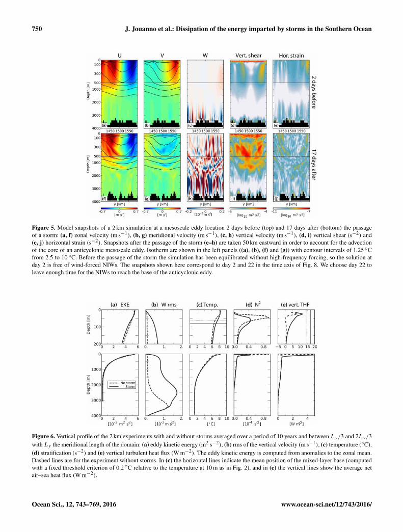
Figure 5. Model snapshots of a 2 km simulation at a mesoscale eddy location 2 days before (top) and 17 days after (bottom) the passageof a storm: (a, f) zonal velocity (m s−1), (b, g) meridional velocity (m s−1), (c, h) vertical velocity (m s−1), (d, i) vertical shear (s−2) and(e, j) horizontal strain (s−2). Snapshots after the passage of the storm (e–h) are taken 50 km eastward in order to account for the advectionof the core of an anticyclonic mesoscale eddy. Isotherm are shown in the left panels ((a), (b), (f) and (g)) with contour intervals of 1.25 ◦Cfrom 2.5 to 10 ◦C. Before the passage of the storm the simulation has been equilibrated without high-frequency forcing, so the solution atday 2 is free of wind-forced NIWs. The snapshots shown here correspond to day 2 and 22 in the time axis of Fig. 8. We choose day 22 toleave enough time for the NIWs to reach the base of the anticyclonic eddy.

Figure 6. Vertical profile of the 2 km experiments with and without storms averaged over a period of 10 years and between Ly/3 and 2Ly/3with Ly the meridional length of the domain: (a) eddy kinetic energy (m2 s−2), (b) rms of the vertical velocity (m s−1), (c) temperature (◦C),(d) stratification (s−2) and (e) vertical turbulent heat flux (W m−2). The eddy kinetic energy is computed from anomalies to the zonal mean.Dashed lines are for the experiment without storms. In (c) the horizontal lines indicate the mean position of the mixed-layer base (computedwith a fixed threshold criterion of 0.2 ◦C relative to the temperature at 10 m as in Fig. 2), and in (e) the vertical lines show the average netair–sea heat flux (W m−2).



Figure 7. Eulerian mean streamfunction ψ (a, b), MOC stream-function diagnosed in isopycnal coordinates (c ,d) and projectedback to depth coordinates (e, f) from 10-year long 2 km equilibratedsimulations with (right) and without storms (left). Units are Sv andthe contour interval is 0.25 Sv. Temperature contours correspondingto 2, 4, 6, 8, 10, 12 and 14 ◦C are indicated in (c, d). Positive cellsare clockwise. The dashed lines in (c, d) represent the 10, 50 and90 % isolines of the cumulative probability density function for sur-face temperature (following Abernathey et al., 2011), which indi-cate how likely a particular water mass is to be found at the surfaceexposed to diabatic transformation. Dotted lines in (e, f) represent(from top to bottom) the 90, 50 and 10 % isolines of the cumula-tive probability density function for mixed-layer depth. The verti-cal dashed line at y = 2850 km represents the limit of the northernboundary damping area. Model transports have been multiplied by10 in order to scale them to the full Southern Ocean.

it is of no concern for our purpose. In the 2 km referencecase without storms, the transport by the main clockwise cellof the MOC streamfunction results in a realistic overturningrescaled value of 18 Sv (Table 2).

Table 2. Maximum of the clockwise cell (as in the context ofFig. 7) of the overturning streamfunction ψiso (Sv) averaged be-tween y = 2000 km and y = 2500 km. The streamfunctions havebeen computed using 10 years of 5-day average outputs from equi-librated experiments. Model transports have been multiplied by 10in order to scale them to the full Southern Ocean.

20 km 5 km 2 km

No storm 20.4 Sv 19.4 Sv 18.0 SvStorms 20.7 Sv 20.9 Sv 21.0 Sv

4 Single-storm effect

As a first step, it is useful to consider a situation in whicha single storm disrupts the quasi-equilibrated flow describedin the previous section so that high-frequency forcing effectscan be more easily identified. The storm is chosen to traveleastward through the center of the domain. The experimentis thoroughly described in Sect. 2 and the ocean spin-downresponse is analyzed in Figs. 5, 8, 9 and 10 for a period of70 days (the storm starts at day 3 and ends at day 7).

4.1 NIW generation and propagation

After the passage of the storm, the horizontal currents be-tween the surface and 1500 m exhibit a layered structure withtypical vertical scales of ∼ 100–200 m (Fig. 5f, g), whichcontrasts with the homogeneity of the mesoscale currents be-fore the passage of the storm (Fig. 5a, b). The layering is sim-ilar to that observed in a section across a Gulf Stream warmcore ring by Joyce et al. (2013). It is associated with an in-crease of the horizontal and vertical shear in the ocean inte-rior (Fig. 5i, j). In agreement with Danioux et al. (2011), weencounter that the storm intensifies the vertical velocities inthe whole water column (Fig. 5h). In response to the storm,KE in the upper 100 m is strongly increased during 5 days(Fig. 8a). An intensification of KE is also observed in the fol-lowing days at depths below 500 m, indicative of downwardpropagation of the energy. A large part of the additional en-ergy injected by the storm occurs in the near-inertial range(Fig. 8b): the space–time distribution of the near-inertial en-ergy (colors) matches rather well the difference of KE be-tween the experiment with a storm and a control experimentwithout a storm starting from exactly the same initial condi-tions (contours).

The near-inertial energy propagates downward and its sig-nature can still be observed 60 days after the storm passagewith two weak maxima: one at the surface and another cen-tered near 1500 m. Over the earlier part of the simulation, wefind downward energy propagation speeds ∼ 25 m day−1 inthe upper 100 and ∼ 90 m day−1 between 100 and 1500 m.These values are higher than the 13 m day−1 average prop-agation speed estimated by Alford et al. (2012) from obser-vations at station Papa, but are within the 10–100 m day−1



(b) KE NIW (c) W rms(a) KE (d) (e) (f ) spectra

day

Figure 8. Response of the ocean to the passage of a single storm: (a) horizontal kinetic energy (log10 m2 s−2), (b) horizontal kinetic energyin the NIW band (colors, log10 m2 s−2) and difference of horizontal kinetic energy between the simulation with storms and a reference

simulation without storms (iso-contours), (c) rms of the vertical velocity (10−4 m s−1) defined as√⟨w2⟩, where τθ = τmax

Rr is the horizontal

average operator, (d) εv energy dissipation due to vertical diffusion (W kg−1) and (e) εh the energy dissipation due to horizontal diffusion(W kg−1). These diagnostics are spatially averaged between Ly/3 and 2Ly/3. The spatially averaged power spectra of the meridionalvelocity (log10 m2 s−2 day−1) is shown in (f) and has been computed using hourly data from day 0 to day 70. The storm starts at day 3 andends at day 7.

range estimated by Cuypers et al. (2013) for NIW packetsforced by tropical storms in the Indian Ocean. Vertical veloc-ities are generally intensified in the depth range where strat-ification is weakest but the maximum of rms vertical veloc-ities qualitatively follows a similar behavior as near-inertialKE: it peaks at 2000 m depth a few days after the storm ini-tiation, and then propagates downward the following weeks(Fig. 8c).

Rotatory polarization of the near-inertial waves is use-ful to separate the upward- and downward-propagating con-stituents of the waves. Rotatory spectra (details of themethodology are given in Appendix B) of the stretched pro-files of velocity allow for a separation of the clockwise (CW)and counter-clockwise (CCW) contributions to the energyas a function of time and vertical wavenumber (Fig. 9a, b).Most of the energy is contained in the CW part of the spec-tra, i.e., most of the energy propagates downward. While theenergy directed downward and contained in wavelengths be-tween 1000 and 2000 m remains strong for about 30 days, theenergy at short wavelengths (< 500 m) is rapidly dissipatedboth for downward- and upward-propagating NIWs. Thenear-inertial KE computed from Wentzel–Kramers–Brillouin(WKB)-stretched CW and CCW velocities (see Appendix Bfor details) are shown in Fig. 9c and d. Between days 20and 30, the KE of CCW waves exhibits a maximum cen-tered around 1500–2000 m. Because the highest topographicfeatures only reach up to 3000 m depth; furthermore, sincenear-inertial velocities have been WKB scaled, we interpretthis local maximum as the signature of interior reflection.During the 5 days following the passage of the storm, wenotice a slight increase of both CW and CCW KE below2500 m depth, suggesting NIW generation at the bottom in

response to storm forcing. Associated energy levels are lim-ited (< 10−2 m2 s−2) and no sign of vertical propagation isobserved so this process must be of minor importance, com-pared to other flow–topographic interactions acting in thesame depth range such as lee-wave generation by the bal-anced circulation (Nikurashin and Ferrari, 2010).

Horizontal velocity frequency spectra computed at eachdepth and averaged over the entire 70-day period of the ex-periment are shown in Fig. 8f. They exhibit energy peaksat f , 2f and to a lesser extent 3f . The near-inertial andsuper-inertial peaks are surface intensified but have a signa-ture throughout the water column. Waves with super-inertialfrequency arise after a few inertial oscillations and are exitedby non-linear wave–wave interactions (Danioux et al., 2008).

4.2 Dissipation of the NI energy

We now turn to the identification of the processes (eitherphysical or numerical) that dissipate the kinetic energy im-parted by the storm. To this end, the complete energetic bal-ance of the single-storm experiment is compared with thatof a control experiment without a storm (Fig. 10). After65 days, the experiment with storm returns to a horizontal ki-netic energy level identical to that of the control experiment(Fig. 10a). The e-folding timescale for the dissipation of ver-tically integrated KE imparted by the storm is ∼ 20 days, butit only reaches 5 days for surface KE. The surface value isconsistent with estimates from drifter observations at simi-lar latitudes (Park et al., 2009). The different contributions ofthe right-hand side of the kinetic energy equation (Eq. 1) thatbalance the input of energy by the wind work are shown inFig. 10b. First we note that the cumulated wind work steadilyincreases after the storm passage (centered at day 5). This



Figure 9. Temporal evolution of clockwise (CW) and counter-clockwise (CCW) spectra as a function of vertical wavelength, com-puted from Wentzel–Kramers–Brillouin (WKB)-stretched near-inertial velocities (a, b) for the single-storm experiment. Units arem2 s−2 cpm−1. Near-inertial KE computed as a function of timeand depth from CW- and CCW-stretched velocities are shown in (c)and (d). Units are m2 s−2.

is due to a slight strengthening of the large-scale eastwardsurface current in response to the storm (not shown). Thisstrengthening is a consequence of the zonal current distribu-tion as a function of latitude, which is not symmetric with re-spect to y = 1500 km, so the domain average additional zonalwind work imparted by the storm is nonzero and positive.At day 70, 61.4 % of the kinetic energy has been dissipatedby diffusive processes in the upper 200 m, while 11.1 % hasbeen dissipated between 200 and 2000 m and 4.3 % between2000 m and the bottom (see Table 3). Bottom friction (5.9 %)and pressure gradients (5.5 %) are also limited sinks for theenergy imparted by the storm. The cumulated contributionsof horizontal advection and Coriolis forces are small com-pared to the other terms (< 1 %). The contribution of the Cori-olis force to the energy budget is not precisely zero due to thestaggered location of u and v points in our Arakawa C-grid.Most of the dissipation due to viscous processes is achievedby vertical processes in the upper 200 m (80 %, Fig. 10c).The maximum contribution of horizontal dissipation is be-tween 200 and 2000 m where it is stronger than vertical dis-sipation (Fig. 10c).

Figure 10. Domain-averaged response of the ocean to the passageof a storm from the same experiment already described in Figs. 5, 8and 9. In order to isolate the response of the storm, we show here thedifferences with a reference experiment without storm and startingfrom exactly the same initial conditions. (a) Horizontal kinetic en-ergy (m2 s−2) computed directly from model velocity (bold black)and indirectly from the time integral of kinetic energy tendencycomputed online before (red) and after (dotted red) Asselin time fil-tering. (b) Cumulated contribution of the different terms of the KEequation (DIFF represent the sum of both horizontal and verticaldissipations). (c) Cumulated lateral (Eh) and vertical (Ev) energydissipation integrated in different depth ranges. (d) Cumulated dis-sipation of energy by the Asselin time filter integrated in differentdepth ranges. (e) Meridional distribution of cumulative wind work,viscous dissipation, bottom friction, horizontal pressure gradientsand Asselin energy dissipation at day 70.



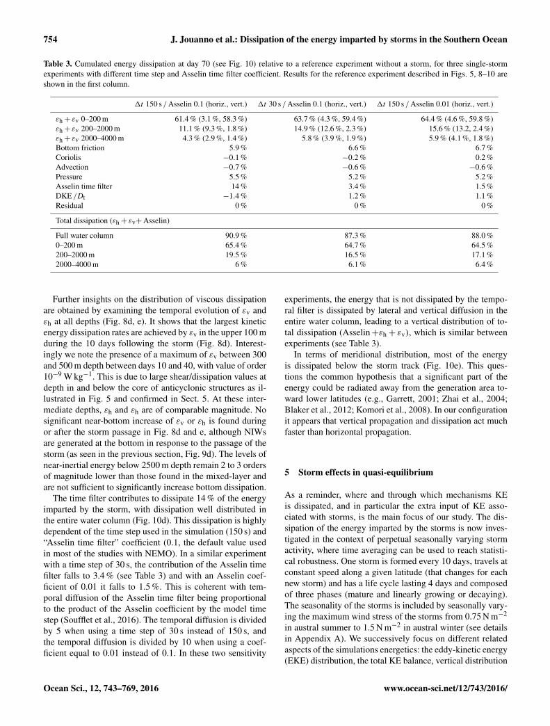
Table 3. Cumulated energy dissipation at day 70 (see Fig. 10) relative to a reference experiment without a storm, for three single-stormexperiments with different time step and Asselin time filter coefficient. Results for the reference experiment described in Figs. 5, 8–10 areshown in the first column.

1t 150 s /Asselin 0.1 (horiz., vert.) 1t 30 s /Asselin 0.1 (horiz., vert.) 1t 150 s /Asselin 0.01 (horiz., vert.)

εh+ εv 0–200 m 61.4 % (3.1 %, 58.3 %) 63.7 % (4.3 %, 59.4 %) 64.4 % (4.6 %, 59.8 %)εh+ εv 200–2000 m 11.1 % (9.3 %, 1.8 %) 14.9 % (12.6 %, 2.3 %) 15.6 % (13.2, 2.4 %)εh+ εv 2000–4000 m 4.3 % (2.9 %, 1.4 %) 5.8 % (3.9 %, 1.9 %) 5.9 % (4.1 %, 1.8 %)Bottom friction 5.9 % 6.6 % 6.7 %Coriolis −0.1 % −0.2 % 0.2 %Advection −0.7 % −0.6 % −0.6 %Pressure 5.5 % 5.2 % 5.2 %Asselin time filter 14 % 3.4 % 1.5 %DKE /Dt −1.4 % 1.2 % 1.1 %Residual 0 % 0 % 0 %

Total dissipation (εh+ εv+Asselin)

Full water column 90.9 % 87.3 % 88.0 %0–200 m 65.4 % 64.7 % 64.5 %200–2000 m 19.5 % 16.5 % 17.1 %2000–4000 m 6 % 6.1 % 6.4 %

Further insights on the distribution of viscous dissipationare obtained by examining the temporal evolution of εv andεh at all depths (Fig. 8d, e). It shows that the largest kineticenergy dissipation rates are achieved by εv in the upper 100 mduring the 10 days following the storm (Fig. 8d). Interest-ingly we note the presence of a maximum of εv between 300and 500 m depth between days 10 and 40, with value of order10−9 W kg−1. This is due to large shear/dissipation values atdepth in and below the core of anticyclonic structures as il-lustrated in Fig. 5 and confirmed in Sect. 5. At these inter-mediate depths, εh and εh are of comparable magnitude. Nosignificant near-bottom increase of εv or εh is found duringor after the storm passage in Fig. 8d and e, although NIWsare generated at the bottom in response to the passage of thestorm (as seen in the previous section, Fig. 9d). The levels ofnear-inertial energy below 2500 m depth remain 2 to 3 ordersof magnitude lower than those found in the mixed-layer andare not sufficient to significantly increase bottom dissipation.

The time filter contributes to dissipate 14 % of the energyimparted by the storm, with dissipation well distributed inthe entire water column (Fig. 10d). This dissipation is highlydependent of the time step used in the simulation (150 s) and“Asselin time filter” coefficient (0.1, the default value usedin most of the studies with NEMO). In a similar experimentwith a time step of 30 s, the contribution of the Asselin timefilter falls to 3.4 % (see Table 3) and with an Asselin coef-ficient of 0.01 it falls to 1.5 %. This is coherent with tem-poral diffusion of the Asselin time filter being proportionalto the product of the Asselin coefficient by the model timestep (Soufflet et al., 2016). The temporal diffusion is dividedby 5 when using a time step of 30 s instead of 150 s, andthe temporal diffusion is divided by 10 when using a coef-ficient equal to 0.01 instead of 0.1. In these two sensitivity

experiments, the energy that is not dissipated by the tempo-ral filter is dissipated by lateral and vertical diffusion in theentire water column, leading to a vertical distribution of to-tal dissipation (Asselin+εh+ εv), which is similar betweenexperiments (see Table 3).

In terms of meridional distribution, most of the energyis dissipated below the storm track (Fig. 10e). This ques-tions the common hypothesis that a significant part of theenergy could be radiated away from the generation area to-ward lower latitudes (e.g., Garrett, 2001; Zhai et al., 2004;Blaker et al., 2012; Komori et al., 2008). In our configurationit appears that vertical propagation and dissipation act muchfaster than horizontal propagation.

5 Storm effects in quasi-equilibrium

As a reminder, where and through which mechanisms KEis dissipated, and in particular the extra input of KE asso-ciated with storms, is the main focus of our study. The dis-sipation of the energy imparted by the storms is now inves-tigated in the context of perpetual seasonally varying stormactivity, where time averaging can be used to reach statisti-cal robustness. One storm is formed every 10 days, travels atconstant speed along a given latitude (that changes for eachnew storm) and has a life cycle lasting 4 days and composedof three phases (mature and linearly growing or decaying).The seasonality of the storms is included by seasonally vary-ing the maximum wind stress of the storms from 0.75 N m−2

in austral summer to 1.5 N m−2 in austral winter (see detailsin Appendix A). We successively focus on different relatedaspects of the simulations energetics: the eddy-kinetic energy(EKE) distribution, the total KE balance, vertical distribution



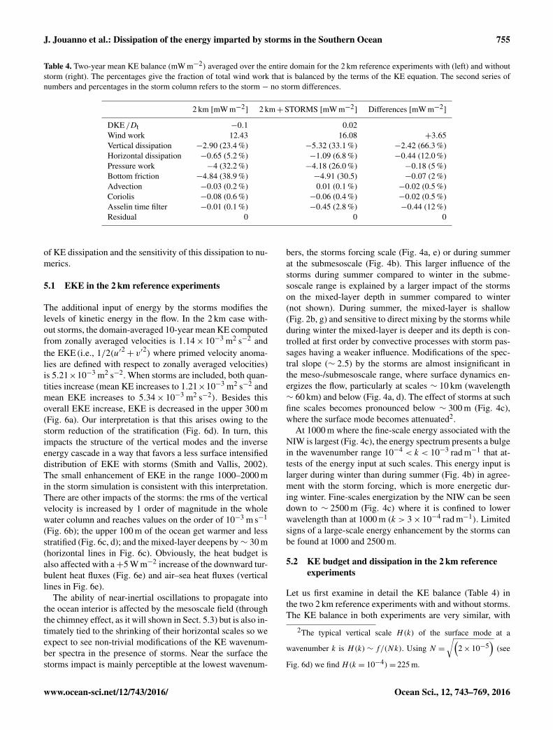
Table 4. Two-year mean KE balance (mW m−2) averaged over the entire domain for the 2 km reference experiments with (left) and withoutstorm (right). The percentages give the fraction of total wind work that is balanced by the terms of the KE equation. The second series ofnumbers and percentages in the storm column refers to the storm − no storm differences.

2 km [mW m−2] 2 km+STORMS [mW m−2] Differences [mW m−2]

DKE /Dt −0.1 0.02Wind work 12.43 16.08 +3.65Vertical dissipation −2.90 (23.4 %) −5.32 (33.1 %) −2.42 (66.3 %)Horizontal dissipation −0.65 (5.2 %) −1.09 (6.8 %) −0.44 (12.0 %)Pressure work −4 (32.2 %) −4.18 (26.0 %) −0.18 (5 %)Bottom friction −4.84 (38.9 %) −4.91 (30.5) −0.07 (2 %)Advection −0.03 (0.2 %) 0.01 (0.1 %) −0.02 (0.5 %)Coriolis −0.08 (0.6 %) −0.06 (0.4 %) −0.02 (0.5 %)Asselin time filter −0.01 (0.1 %) −0.45 (2.8 %) −0.44 (12 %)Residual 0 0 0

of KE dissipation and the sensitivity of this dissipation to nu-merics.

5.1 EKE in the 2 km reference experiments

The additional input of energy by the storms modifies thelevels of kinetic energy in the flow. In the 2 km case with-out storms, the domain-averaged 10-year mean KE computedfrom zonally averaged velocities is 1.14× 10−3 m2 s−2 andthe EKE (i.e., 1/2(u′2+ v′2) where primed velocity anoma-lies are defined with respect to zonally averaged velocities)is 5.21×10−3 m2 s−2. When storms are included, both quan-tities increase (mean KE increases to 1.21×10−3 m2 s−2 andmean EKE increases to 5.34× 10−3 m2 s−2). Besides thisoverall EKE increase, EKE is decreased in the upper 300 m(Fig. 6a). Our interpretation is that this arises owing to thestorm reduction of the stratification (Fig. 6d). In turn, thisimpacts the structure of the vertical modes and the inverseenergy cascade in a way that favors a less surface intensifieddistribution of EKE with storms (Smith and Vallis, 2002).The small enhancement of EKE in the range 1000–2000 min the storm simulation is consistent with this interpretation.There are other impacts of the storms: the rms of the verticalvelocity is increased by 1 order of magnitude in the wholewater column and reaches values on the order of 10−3 m s−1

(Fig. 6b); the upper 100 m of the ocean get warmer and lessstratified (Fig. 6c, d); and the mixed-layer deepens by∼ 30 m(horizontal lines in Fig. 6c). Obviously, the heat budget isalso affected with a+5 W m−2 increase of the downward tur-bulent heat fluxes (Fig. 6e) and air–sea heat fluxes (verticallines in Fig. 6e).

The ability of near-inertial oscillations to propagate intothe ocean interior is affected by the mesoscale field (throughthe chimney effect, as it will shown in Sect. 5.3) but is also in-timately tied to the shrinking of their horizontal scales so weexpect to see non-trivial modifications of the KE wavenum-ber spectra in the presence of storms. Near the surface thestorms impact is mainly perceptible at the lowest wavenum-

bers, the storms forcing scale (Fig. 4a, e) or during summerat the submesoscale (Fig. 4b). This larger influence of thestorms during summer compared to winter in the subme-soscale range is explained by a larger impact of the stormson the mixed-layer depth in summer compared to winter(not shown). During summer, the mixed-layer is shallow(Fig. 2b, g) and sensitive to direct mixing by the storms whileduring winter the mixed-layer is deeper and its depth is con-trolled at first order by convective processes with storm pas-sages having a weaker influence. Modifications of the spec-tral slope (∼ 2.5) by the storms are almost insignificant inthe meso-/submesoscale range, where surface dynamics en-ergizes the flow, particularly at scales ∼ 10 km (wavelength∼ 60 km) and below (Fig. 4a, d). The effect of storms at suchfine scales becomes pronounced below ∼ 300 m (Fig. 4c),where the surface mode becomes attenuated2.

At 1000 m where the fine-scale energy associated with theNIW is largest (Fig. 4c), the energy spectrum presents a bulgein the wavenumber range 10−4 < k < 10−3 rad m−1 that at-tests of the energy input at such scales. This energy input islarger during winter than during summer (Fig. 4b) in agree-ment with the storm forcing, which is more energetic dur-ing winter. Fine-scales energization by the NIW can be seendown to ∼ 2500 m (Fig. 4c) where it is confined to lowerwavelength than at 1000 m (k > 3× 10−4 rad m−1). Limitedsigns of a large-scale energy enhancement by the storms canbe found at 1000 and 2500 m.

5.2 KE budget and dissipation in the 2 km referenceexperiments

Let us first examine in detail the KE balance (Table 4) inthe two 2 km reference experiments with and without storms.The KE balance in both experiments are very similar, with

2The typical vertical scale H(k) of the surface mode at a

wavenumber k is H(k)∼ f/(Nk). Using N =√(

2× 10−5)

(see

Fig. 6d) we find H(k = 10−4)= 225 m.



Figure 11. Kinetic energy dissipation (ε; W kg−1) as a function of depth in experiments at 2 km with storms (continuous lines) and withoutstorms (dashed lines): total energy dissipation ε with and without storms (a), dissipation due to vertical processes εv and dissipation due tohorizontal processes εh (b), εh computed from a second-order (UBS-C2) or fourth-order (UBS-C4) centered scheme (see text for details)together with a 20-year mean and standard deviation of ε for the 2 km reference experiment (c), and summer (December–January–February)and winter (June–July–August) ε. Profiles are computed using 5-day snapshots of the entire domain for a 2-year period. Position, strengthand duration of the storms remain strictly equal in the different experiments.

overall wind work mainly balanced by the work done by bot-tom friction (38.9 % without storms and 30.5 % with storms),pressure work maintaining the system available potential en-ergy (32.2, 26.0 %) and vertical diffusion (23.4, 33.1 %). TheKE balance also indicates that the additional input of en-ergy provided by the storms (+3.64 mW m−2) is balancedat 90 % by dissipation (−2.86 mW m−2 for horizontal andvertical dissipation to which one should add the Asselin filtercontribution) with pressure work and bottom friction beingsecondary (−0.18 mW m−2 representing a 5 % contributionand−0.07 mW m−2 representing a 2 % contribution). This isin stark contrast with the equilibration of the low-frequencywind work feeding the balanced circulation.

Now let us focus on the spatial and seasonal distributionof the horizontal and vertical KE dissipation terms εh and εv.The vertical distribution of these terms are computed usinginstantaneous outputs available every 5 days during the last2-year of the 2 km runs. This choice of a limited 2-year pe-riod is justified given the smallness of the standard deviationof annual mean ε computed using 20 years of simulation ofthe experiment with storms (Fig. 11c), e.g., compared to εdifferences we present for different experiments. As statedin Sect. 2, we estimate UP3 intrinsic horizontal diffusivityas the difference between UP3 momentum tendency and thetendency given by a fourth-order advective scheme. The al-

ternative use of a second-order advection scheme producesvery similar estimates of εh (Fig. 11c).

Overall energy dissipation (ε = εh+ εv) in the referenceexperiments is increased by 1 order of magnitude or moreover most of the water column in the presence of storms(Fig. 11a). Exception is found in the lowest 1000 m, wheredissipation is always strong because of the interaction of themesoscale and large-scale field with the topography. Withoutstorms, dissipation reaches a minimum of 3× 10−12 W kg−1

between 1000 and 1500 m depth while the presence of stormsincreases the level of dissipation to > 10−10 W kg−1 in thisdepth range, in agreement with the results for the single-storm experiment (Fig. 8).

The distribution of the dissipation between horizontal andvertical diffusive processes and their respective sensitivityto the energy input by the storms reveals some interest-ing behavior. First, vertical dissipation dominates in the up-per 200 m and (less clearly) below 3000 m, but in between,horizontal processes account for most of the dissipation(Fig. 11b). This is particularly true for the experiment withstorms in which εv is systematically less than 1/4 of εh be-low 200 m. Second, there is an increase of horizontal dissipa-tion in the interior in response to the storms (Fig. 11b). Thisis consistent with enhanced energy at short wavelengths (λ< 60 km, Fig. 4a, c).



Figure 12. εh and εv (W kg−1) distribution within composite cyclones (top) and anticyclones (bottom) identified in the 2 km experimentswithout storms (left) and with storms (right). The black iso-contours are isotherms from 2 to 8 ◦C and σ/f iso-contours are shown in white(0.9, 0.95 and 0.98 σ/f ), with σ = f + ξ/2 the effective frequency and ζ the relative vorticity. Composites are built using 10 years of 5-day-averaged model outputs, between Ly/3 and 2Ly/3. A total of 8167 cyclone and 8878 anticyclone snapshots have been identified in theexperiment without storms and 7306 cyclone and 8037 anticyclone snapshots in the experiment with storms.

Since the air–sea heat fluxes and the strength of the stormsfollow a seasonal cycle, we expect some seasonality of bothnear-surface and interior dissipation. This is examined bycomparing ε profile in summer and winter (Fig. 11d). Val-ues of ε in the upper 300 m display large differences be-tween summer and winter, in both experiments with or with-out storms. Increased upper-ocean energy dissipation duringwinter is explained by mixed-layer convection in response tosurface heat loss. Below 300m, the experiment with stormsis the only one that displays seasonal variations of ε, withgreatest values during winter. This is consistent with obser-vations by Wu et al. (2011), who observed a seasonal cycleof diapycnal diffusivity (hence of ε) in the Southern Ocean atdepths down to 1800 m, although it reaches somewhat deeper(∼ 2500 m) in our solutions.

5.3 How do mesoscale eddies shape KE dissipation?

Mesoscale activity is known to affect NIW penetration intothe ocean interior (Danioux et al., 2011). In order to clarifythe role of mesoscale structures on energy dissipation distri-bution, an eddy detection method is used to produce com-posite averages of dissipation, relative to eddy centers. Theidentification of the eddies is based on a wavelet decomposi-tion of the surface vorticity field (e.g., Doglioli et al., 2007).Following Kurian et al. (2011) a shape test with an error cri-

terion of 60 % is used to discard structures with shapes toodifferent from circular. Since the Rossby radius of deforma-tion varies meridionally within the model domain, compos-ites are built with eddies located between Ly/3 and 2Ly/3,and with an area larger than 400 km2. The barycenter is takenas the center of the eddies and used as reference point to buildthe composites.

The general distribution of εh and εv within composite ed-dies (Fig. 12) is in agreement with the vertical distributionof domain-averaged ε discussed in the previous section, withincreased values of εh and εv near the surface and the bottom.But the composites also highlight the impact of eddies on thedistribution of εh and εv. As discussed below the distributionof the kinetic energy dissipation within eddies is very differ-ent depending on the presence or absence of storms.

Without storms, the distribution of either εh and εv in theupper 1500 m shows that the border of the cyclones and anti-cyclones are hot spots of dissipation, while the dissipation atthe center of the eddies is weaker than outside (Fig. 12a–d).This was expected since horizontal strain and vertical shearare largest at the edges of eddies and weak within the eddies.Near the bottom, dissipation is increased below the cyclonescenters (Fig. 12a, b) and decreased below the anticyclones(Fig. 12c, d), owing to increased near-bottom velocities incyclones compared to anticyclones (not shown).



Figure 13. Kinetic energy dissipation (ε; W kg−1) as a function of depth in experiments at 20, 5, 2 and 1 km horizontal resolution, withstorms (continuous lines) and without storms (dashed lines): total energy dissipation ε with storms (a) and without storms (b), dissipationdue to vertical processes εv with storms (c) and without storms (d), dissipation due to horizontal processes εh with storms (e) and withoutstorms (f), and the fraction of the total dissipation due to vertical processes (εv/ε in %) (g and h). As in Fig. 11, profiles are computed using5-day snapshots of the entire domain for a 2-year period. Position, strength and duration of the storms remain strictly equal in the differentexperiments. The experiment z320 has an horizontal resolution of 2 km but 320 vertical levels, ranging from 1 m at the surface to 250 m atthe bottom (below 2500 m depth the vertical size of the cells is the same as in the 2 km reference experiment).

In the presence of storms (Fig. 12e–h), εv and εh peakat the base of the anticyclones with values higher than10−9 W kg−1, in qualitative agreement with various observa-tions of NIW trapping at the base of the anticyclones (Joyceet al., 2013; Kunze et al., 1995). The largest dissipation isbounded by the contour σ = 0.95f with σ = f +ξ/2 the ef-fective frequency. The compositing highlights the dispropor-tionate importance of anticyclones for NIW dissipation. Thetotal area occupied by the anticyclones that have been pickedup by the eddy detection method represents only 2.6 % each

of the domain area, but concentrate the interior KE dissi-pation at depth. Between 300 and 1500 m, 5 % of εh and17 % of εv is achieved within identified anticyclones. Con-versely, cyclone which statistically occupy a similar area ofthe model domain are associated with only 4 % of εh and1.9 % of εv. The statistical importance of anticyclones is fur-ther discussed in the conclusion.



Figure 14. Kinetic energy dissipation (ε) and wind work as a function of model resolution, in experiments with (continuous lines) and withoutstorms (dashed lines): (a) wind work and energy dissipation integrated from surface to bottom (mW m−2), (d) energy dissipation integratedfrom surface to bottom (decomposed into contributions from ε, bottom friction and Asselin time filter; mW m−2) and total dissipation ε(W kg−1) averaged in the depth ranges 0–100 m (b), 100–400 m (c), 400–1000 m (d) and 1000–2000 m (e). Values are computed using 5-daysnapshots of the entire domain for a 2-year period as in Fig. 9. Isolated dots represent ε for the 2 km experiment with 320 vertical levels.Wind work (a) and energy dissipation contributions (d) have only been computed for the 20, 5 and 2 km experiments.

5.4 Sensitivity tests

How dissipation changes when key physical and numericalparameters are varied is examined below.

Horizontal resolution. Energy dissipation is compared inexperiments at 20, 5, 2 and 1 km horizontal resolution(Fig. 13). The sensitivity to resolution strongly dependson the considered depth range. Near the surface (0–100 m) the dissipation is almost not sensitive to the res-olution (Figs. 13a, b and 14b). This is coherent withthe relatively weak variations of the wind work fromone resolution to another (Fig. 14a). But below (100–400 m), experiments with or without storms show a de-crease of ε when increasing resolution (Figs. 13a, band 14c). This decrease is not related to modificationsof the wind work (Fig. 14a) and occurs in a depth rangeaffected by upper-ocean convection. So it may mostlyresult from the weakening of the dissipation due toupper-ocean convection when resolution increases, ashighlighted by the shallowing of the mixed-layer depth(with storms and (without storms): 101 m (93 m) at1x = 20 km, 87 m (67 m) at 1x = 5 km, 80 m (59 m) at1x = 2 km and 68 m (53 m) at1x = 1 km). This wouldbe in agreement with the re-stratifying effect of themesoscale and sub-mesoscale flow, which become moreefficient when resolution increases (e.g., Fox-Kemper,2008; Marchesiello et al., 2011).

In the depth range 400–3000 m, the sensitivity to reso-lution is highly dependent on the presence or absence ofstorms. Without storms, a major reduction of dissipationwith increasing resolution is noticeable (Fig. 13b). This

reduction is of a factor 10 or more in the depth range400–2000 m, when going from 20 to 1 km resolution(Figs. 13b and 14c, e, f). Concomitantly, the fractionof dissipation due to vertical shear increases becausethat corresponding to lateral shear drops most rapidly(Fig. 13h). At 1km resolution, it is systematically above20 % down to ∼ 2000 m and reaches 50 % at 1500 mdepth. This contrasts with the run at 20 km where εvis never more than 7 % of the total dissipation over thesame depth range.

The behavior of interior dissipation with storms is strik-ingly different. Dissipation changes with resolution aremuch more modest (in log scale). As mentioned before,dissipation in the upper 100–400 m decreases when go-ing from 1x = 20 to 1 km (Fig. 14c). Between ∼ 400and 2000 m, increasing resolution tends to increase dis-sipation (Figs. 13a and 14d, e). At 20 km the mesoscalefield is not well resolved and weaker; therefore, themesoscale near-inertial vertical pump is less efficientin transferring the near-inertial energy into the interior;5 km resolution changes total dissipation significantly(e.g., from 4×10−11 to 1.2×10−10 W kg−1 in the depthrange 1000–2000 m, Figs. 13a and 14f). Changes aremodest beyond 1x = 5 km. This is because horizontaldissipation remains nearly unchanged and dominates to-tal dissipation. On the other hand, vertical dissipationexhibits interesting changes in this resolution range. Inparticular, it keeps increasing and so does its overallfraction in total dissipation. Also it develops a weak rel-ative maximum around 300–500 m at 1 and 2 km. We



relate this maximum to the one seen in dissipation com-posites for anticyclones (Fig. 12).

Near the bottom important changes also take place whenincreasing resolution: vertical (horizontal) dissipationdecreases (increases), which leads to a slight decreasein dissipation by interior viscous processes. Instead, dis-sipation by bottom friction increases significantly withresolution (Fig. 14d). We are not sure how to inter-pret these bottom sensitivities, especially since we donot properly resolve the processes implicated in flow–topography interactions (Nikurashin and Legg, 2011).

Vertical resolution. An experiment with 320 vertical lev-els has been carried out in which vertical shears (andhigh-order vertical modes) are better represented thanwith the reference 50 levels. The vertical thickness ofthe cells increases from 2 m at the surface, 5 m at 500 mdepth, 70 m at 1000 m depth and 180 m near the bot-tom. The size of the cells below 2500 m are equal to thereference experiment so that the local characteristics offlow–topography interactions are unchanged. The over-all dissipation ε is increased in the presence of storms inthe interior in the configuration with 320 vertical levels(Figs. 13a, b and 14c–e), indicating that the downwardpropagation of the NIE is better resolved in the highvertical resolution experiment with more NIE availableat depth. A similar increase of ε in the upper 100 m inthe experiments with and without storms (Fig. 14b) sug-gests that mixed-layer dynamics is profoundly alteredwhen changing the vertical resolution.

Advection schemes. The reference experiment relies on anUP3 advection scheme (Webb et al., 1998). It is com-pared with three experiments run with three widely usedadvection scheme: the QUICK (Quadratic Upstream In-terpolation for Convective Kinematics) scheme, whichis the default scheme of The regional oceanic modelingsystem (ROMS) model (Shchepetkin and McWilliams,2005) and also includes implicit diffusion; a second-order centered scheme with a horizontal biharmonicviscosity of −109 m4 s−2; and a second-order centeredscheme with the vector invariant form of the momen-tum equations (Madec, 2014) with the same horizontalbiharmonic viscosity. The implicit dissipation of UP3and QUICK take the form of a biharmonic operatorwith an eddy coefficient proportional to the velocity(Ah =−|u|1x

3/12 with UP3 and Ah =−|u|1x3/16

with QUICK). Although QUICK is by construction lessdissipative compared to UP3, ε in both experiments arevery similar (Fig. 15a). With or without storms, thesecond-order scheme in flux form (CEN2) or vector in-variant form (VFORM) leads to increased ε in the oceaninterior with the increase being the largest at the bottom(the energy dissipation profiles for the second-order andthe vector-form scheme are so close that they are su-

perimposed in Fig. 15a). Such distribution of the dis-sipation changes is obviously related to the choice ofa biharmonic coefficient of −109 m4 s−2: characteris-tic velocities of 1.5 and 2 m s−1 are required for UP3and QUICK schemes to match a biharmonic diffusioncoefficient of −109 m4 s−2. So near the surface wherecurrents are strong the explicit diffusion in the simula-tions with second-order schemes is of same order as theimplicit diffusion in QUICK/UP3 simulations, while atdepth an explicit biharmonic operator with coefficient−109 m4 s−2 overestimates the diffusion compared toUP3/QUICK implicit diffusion. We also note a dissi-pation increase in the depth range 1000–2000 m whenusing these schemes in the presence of storms. Sensitiv-ity closer to the surface is much more limited.

Maximum wind speed. Stronger winds increase the energydissipation in the interior (Fig. 15c). Changes in dissi-pation levels take place from the near surface down to2500–3000 m, which again highlights that near-inertialenergy is able to propagate down to such depths. Dis-sipation changes induced by modifications of the flow–topography interactions would also yield changes in dis-sipation near the bottom, which is not the case, particu-larly when comparing the 1 and 1.5 N m−2 experiments.

Storm speed. The storm speed of the reference experi-ment was taken as Cs = 15 m s−1, a value close to the12 m s−1 inferred by Berbery and Vera (1996) in someparts of the Southern Ocean. But this speed is expectedto vary from storm to storm and impact the amountof energy deposited into the near-inertial range as sev-eral studies have shown in particular in the contextof hurricanes (Price, 1981; Greatbatch, 1983, 1984).The response of the ocean to storms traveling at 20,15, 10, 5 and 0 m s−1 is compared in Fig. 15b withother storm characteristics (including trajectory) re-maining unchanged. The storms travel exactly at thesame latitude and for the same duration as in the ref-erence experiment with Cs = 15 m s−1. Above 3000 mdepth, energy dissipation increases with storm displace-ment speed until reaching the threshold of 15 m s−1 be-yond which it reduces slightly. These results are consis-tent with those of Greatbatch (1984) and in particularNIE is maximized for a storm timescale L/Cs ∼ (2×500 km) /15 m s−1

∼ 18 h close to the inertial timescale(2π/f ), with L the scale of the storm. Bottom dis-sipation is slightly enhanced (from 2× 10−9 to 3×10−9 W kg−1) when storm speed decreases, presumablyas a result of more energy being injected in the balancedcirculation when storms move slowly.

More importantly we note that major relative changes inenergy dissipation levels occur in the ocean interior as Uvaries, with 1 order of magnitude difference or more forstorms traveling at 5 or 0 m s−1 compared to storm travel-



Figure 15. Sensitivity of energy dissipation (ε) profiles to numerics (a), storm speed (b) and storm strength (c). Experiments with (without)storms are shown with continuous (dashed) lines. The advective schemes tested in (a) are UP3 (reference), QUICK, flux-form second-ordercentered advection scheme (CEN2) and a vector form advection scheme (VFORM). The profiles of the latter two (blue and green colors) areconfounded in panel (a). Dissipation induced by storms traveling at different speeds is tested in (c) for propagation speeds of 0, 5, 10, 15 and20 m s−1. In these experiments the duration and the power of the storms are the same as in the reference experiment (for which the stormpropagation speed is 15 m s−1). In (d), the sensitivity to the storm strength is tested by comparing experiments with maximum wind-stressvalues equal to 1, 1.5 (reference) and 3 N m−2. All the sensitivity experiments are run at 2 km horizontal resolution. They start from the sameinitial condition equilibrated without storms, and they are run for 3 years. Profile are built using 5-day snapshots of the entire domain for thelast 2 years of the simulations.

ing at 15 m s−1 in the depth range 400–2000 m. Importantchanges are also found for U = 10 m s−1, which further con-firms the subtlety of the ocean ringing and its consequences.In particular, note that a 30 % increase or reduction of thestorm displacement speed has more of an effect than a 30 %reduction in storm strength. It also suggests another possiblemodus operandi for low-frequency variability in the atmo-sphere to impact the functioning of the ocean interior througha modification of the storm characteristics such as displace-ment speed.

6 Impact of the storms on the Southern Ocean MOC

KE dissipation and mixing are related in subtle ways.Given the profound modifications of KE dissipation by high-frequency winds presented in the previous sections we nowassess the influence of the storms on the water-mass transfor-mations by examining the MOC sensitivity (Fig. 7). Stormsincrease the clockwise cell intensity by 3 Sv that is a 16 %increase compared to the experiment without storms. Thisshows that in our experiment the storms contribute efficientlyto the strength of the MOC. It is worth mentioning that thereare almost no changes in the mean Ekman drift as suggestedby the very similar Eulerian overturning streamfunction inthe cases with and without storms (Fig. 7a, b).

Both the MOC and the response of the MOC to the stormsare sensitive to model horizontal resolution (Table 2). With-out storms, the maximum (and scaled) value of the MOC de-creases from 20.4 Sv at 20 km to 18.0 Sv at 2 km. This is wellrelated to the decrease of interior (below 100 m) kinetic en-ergy dissipation with resolution increase in the experimentswithout storms (Fig. 13b). But when storms are included, theMOC increases with an amplitude that depends on the reso-lution (+0.3 Sv at 20 km, +1.5 Sv at 5 km, +3.0 Sv at 2 km),leading to transports that are relatively similar between ex-periments (20.7 Sv at 20 km, 20.9 Sv at 5 km and 21.0 Sv at2 km). Again this is in agreement with the sensitivity of thekinetic energy dissipation to model resolution: the presenceof storms increases the levels of energy dissipation in the in-terior to a level, which remains broadly constant at the differ-ent resolutions (Figs. 13a, 14).

The processes that dominate the changes of water-mass transformation in the experiments with and withoutstorms can be identified by means of an analysis followingWalin (1982), Badin and Williams (2013) and other. Water-mass transformation rate G is defined as

G(ρ)=11ρ

∫Dair−seadA−

∂Ddiff

∂ρ



Figure 16. Transformation rate (in Sv): total (a), contribution of air–sea fluxes (b) and diffuse fluxes across isotherms for the 2 km sim-ulations without storms (c) and with storms (d). The diffuse fluxesare separated into vertical (light gray) and lateral (black) contribu-tions. The dashed lines in (c) and (d) correspond to transformationby diffuses fluxes below 300 m depth. Model transports have beenmultiplied by 10 in order to scale them to the full Southern Oceans.

with Ddiff the diffusive density flux and Dair−sea the surfacedensity flux given by

Dair−sea =−α

CpQnet, (4)

where Qnet is the net surface heat flux, Cp the heat capac-ity of the sea water, α the thermal expansion coefficient ofsea water and 1ρ the density integration interval. The di-apycnal volume flux is directed from light to dense waterswhen G is positive. The computation of the different termsis achieved following the technical details provided in Mar-shall et al. (1999) with density bin 1ρ of 0.1 kg m−3. Foreasy comparison with previous results, the diagnostics areperformed in temperature space. As for momentum diffu-sion, the horizontal diffusion of temperature is computed asthe difference between UP3 temperature tendency and thetendency given by a fourth-order centered scheme.

In the 2 km experiments without storms, the transforma-tion by air–sea fluxes is mainly from dense to light watersand peaks at −13 Sv near 6 ◦C (Fig. 16b; again the valueshere are scaled to the full Southern Ocean). At this tempera-ture, the transformation by diffusive processes only reachesa modest −1 Sv (Fig. 16c) and the total transformation rate(∼−14 Sv) is consistent with the 14.5 Sv of meridionallyaveraged MOC transport centered at 6 ◦C (not shown). Thetransformation by diffusive fluxes has two extrema near 4 ◦Cand 12 ◦C, which correspond to temperatures where convec-tion is more active as suggested by the isolines of cumulativedistribution of mixed-layer depth in Fig. 7f or by the seasonalcycle of the mixed-layer depth in Fig. 2b.

Overall, storms increase both the transformation by air–sea fluxes (∼+3 Sv or +25 % at 6 ◦C) and diffusive fluxes(∼+2 Sv or +130 % at 4 ◦C), leading to a ∼+3 Sv totalincrease of water-mass transformation is the isotherm range4–8 ◦C (Fig. 16a) that is consistent with the +3 Sv strength-ening of the main clockwise cell of the MOC. The changein the air–sea fluxes is due to the feedback term that acts torestore model SST toward its prescribed SST climatology.In the presence of storms, the contributions from lateral andvertical diffusion are almost equal (Fig. 16d), while withoutstorms lateral diffusion dominates the water-mass transfor-mation (Fig. 16c). The fraction of transformation achievedbelow 300 m depth is very weak indicating that most of thediffusive transformation process takes place in the near sur-face (Fig. 16c, d). On the other hand, an important caveatis that only ∼ 20 % of the energy dissipated below 300 mis properly connected to mixing (through the k-epsilon sub-model).

7 Discussion

7.1 Model realism and limitations

The realism of model dissipation is difficult to evaluateagainst observations of dissipation rates because of spatialvariability and temporal intermittency in nature (see for ex-ample the longitude dependence of the dissipation rate foundby Wu et al., 2011, in the Southern Ocean; variability at afiner scale is also important). With storms, mean interior dis-sipation values at the highest resolution are in the range 1–10× 10−10 W kg−1 depending on exact depth above 2000 mand season. Such values are consistent with estimates frommicrostructure measurements (Waterman et al., 2013; Sheenet al., 2013) or from release and tracking of dye at mid-depth(Ledwell et al., 2011). However, they are on the lower end ofthe ARGO estimates of Wu et al. (2011).

A source of uncertainty in comparing our simulations toobservations is that we lack internal-gravity wave generationby tides and we also misrepresent the interaction betweenthe geostrophic flow and bottom topography. Both of theseprocesses should significantly contribute to near-bottom dis-



sipation enhancement and their consequences around mid-depth may not be negligible. Cabbeling and thermobaricityare other indirect sources of mixing that are not taken intoaccount in our study.

Assuming that Wu et al. (2011) estimates in regions withsmooth bathymetry primarily reflect dissipation of wind-input energy, we can nonetheless make two important quan-titative remarks. The vertical structure of storm energy dis-sipation in our simulations is qualitatively consistent withtheir observations: we find a factor 5–6 reduction in dissi-pation from 400 to 1800 m depth as they approximately do(their Fig. 3). Model seasonal variations in ε also agree (notethat we infer seasonal changes of ε in Wu et al. (2011) fromchanges in diapycnal diffusivity, assuming that subsurfacestratification does not vary between seasons). Model (respec-tively observations from Wu et al., 2011) winter to summerε ratios decrease from ∼ 2 (∼ 1.8) in the depth range 300–600 m to 1.6 (∼ 1.4) in the depth range 1300–1600 m. Thesenumbers agree within the error bars associated with observa-tions by Wu et al. (2011). On the other hand, it is plausiblethat the slightly weaker seasonal cycle systematically foundin the observations arises from dissipative contributions dueto processes other than wind. The respective roles of windinput and that of a distinct non-seasonally variable processon dissipation could in principle be separated but model un-certainties and limitations should also be kept in mind.

Near the bottom, our simulations generate dissipation atlevels that are essentially unaffected by synoptic wind activ-ity (although this is less true when storms travel slowly). εreaches ∼ 5× 10−9 W kg−1, a value which is not overly af-fected by numerical resolution and turns out to be close tothe values measured or inferred near-rough topography (Wa-terman et al., 2013; Sheen et al., 2013). This being said, im-portant reorganizations in the bottom 500 m from vertical tohorizontal dissipation as horizontal resolution increases sug-gest cautiousness. So does the unrealistic representation ofinternal lee-wave processes.

7.2 Energy pathways

Results by Nikurashin et al. (2013) suggest that the bulk ofthe large-scale wind power input in the Southern Ocean isdissipated at the bottom by the interaction of the mesoscaleeddy field with rough (small-scale) topography. Our simu-lations also show high energy dissipation at the bottom, butinstead of as in the rough experiment described in Nikurashinet al. (2013), for which most of the energy imparted by thewind is balanced by interior viscous dissipation, the wind in-put in our 2 km experiment without storms is balanced bybottom friction (38.9 % associated with unresolved turbu-lence in the bottom boundary layer), pressure work (32.2 %)and interior viscous dissipation (23.4 %). This points out thatwe are not exactly in the same regime as the one describedin Nikurashin et al. (2013). This is probably related to low

roughness of our experiments compared to the rough experi-ment in Nikurashin et al. (2013).

Using a global high-resolution model, Furuichi etal. (2008) estimate that 75–85 % of the global wind energyinput to surface near-inertial motions is dissipated in the up-per 150 m. Similarly, Zhai et al. (2009) analyzing a global1/12◦ model found that nearly 70 % of the wind-inducednear-inertial energy at the sea surface is lost to turbulentmixing within the top 200 m. Our results are in qualitativeagreement with these studies: in our high-resolution simula-tions only ∼ 65–70 % of the overall energy imparted by thestorm is dissipated in the upper 200 m (65 % in the one stormexperiment; see Table 4; 70 % in the multiple storm experi-ment, not shown). Note though that, in contrasts to Furuichiet al. (2008), who base their estimate on the near-inertial re-sponse of the wind energy input, we do not separate the bal-anced and unbalanced response to the storms. A substantialpart of the additional wind work imparted by the storms isnot near-inertial, as revealed by the 1.4 mW m−2 near-inertialwind work in the experiment with storms, which is only afraction of the +3.6 mW m−2 total wind work increase com-pared to the experiment without storms. Since the balancedresponse to the storms does not follow the same pathway to-ward dissipation (see below), such differences between ourresults and Furuichi et al. (2008) are not unexpected.

Using a 1/10◦ model of the Southern Ocean, Rath etal. (2013) found that accounting for the ocean-surface ve-locity dependence of the wind stress decreases the near-inertial wind power input by about 20 % but also damps themixed-layer (ML) near-inertial motions leading to an over-all ∼ 40 % decrease of the ML near-inertial energy. Overall,this damping effect is found to be proportional to the inverseof the ocean-surface mixed-layer depth. In our set of sim-ulations, we do not include any wind-stress dependence onocean-surface velocity, which remains a debated subject (Re-nault et al., 2016). Our main motivation for doing so was toensure that the mean wind stress remains the same betweenthe different model experiments that have been performed inthis study. Nevertheless, we should keep in mind that we missa potentially important dissipative process for the NIWs. Thevertical turbulence model we use does not include an explicitwave description so the surface wave mixing effect is param-eterized and non-local wave breaking, Stokes drift or Lang-muir cells are not considered. These processes modulate themomentum and energy deposited into the ocean as well asnear-surface dissipation rates. For example, the analysis ofa coupled atmosphere–wave–ocean model simulating hurri-cane conditions suggests that the Stokes drift below the stormcan contribute up to 20 % to the Lagrangian flow magnitudeand change its orientation (Curcic et al., 2016). These pro-cesses certainly impact the near-inertial wind energy inputand distribution of its dissipation, and would deserve furtherattention, perhaps using a more realistic (regional) setup.

Finally, our experiments provide an interesting perspec-tive on the dissipation of the energy associated with the slow



versus NIW part of the flow. The ways the energy impartedto the ocean by high and low frequency winds are balanceddiffer markedly as one may have expected. Wind work im-parted by the storms is mainly balanced by viscous dissi-pation (> 80 %), mainly in the upper ocean and to a lesserextent in the interior. Bottom friction (∼ 5 %) and pressurework (∼ 5 %) play a minor role while these two terms arekey in the equilibration of the low-frequency part of the cir-culation (note that the loss term associated with pressuregradient forces represents the potential energy source dueto Ekman pumping). Perhaps more surprisingly, total inte-rior dissipation in the simulation with and without stormspresent distinct sensitivities with respect to resolution. Ashorizontal/vertical resolution increases storm energy dissipa-tion tends to diminish within a few hundred meters belowthe mixed layer base but increases farther down. Conversely,dissipation of the balanced circulation sharply decreases withincreasing resolution over a broad range of depth in the oceaninterior, from below the mixed layer down to 3000 m depth.It is also the situation where convergence is least clear inthe range of resolutions that we explore. Even 1x = 1 kmresolution may still be insufficient to adequately resolvefine-scale dissipative processes affecting the balanced flow(Vanneste, 2013). In any event and far from topographic fea-tures, dissipation of the balanced flow, which is robustly 1to 2 orders of magnitude smaller than dissipation of the NIEbelow 300 m depth, is unlikely to have a substantial effect ondiapycnal mixing in the Southern Ocean interior.

8 Conclusions

Kinetic energy (KE) dissipation and its effect on ocean mix-ing are a subject of intense research. The aim of this studyis to investigate the fate and the overall impact of the en-ergy imparted by the storms in the Southern Ocean. The setof semi-idealized numerical simulations we use to this endallow us to explore and to identify the limitations faced bythe general/regional ocean modeling community in the nu-merical representation of these processes. We also providean additional perspective on the MOC sensitivities (to high-frequency winds) in a semi-idealized representation of theSouthern Ocean that shares important characteristics with theones used in Abernathey et al. (2011), Morrison and Hogg(2013; MOC sensitivity to the mean wind stress) or Morri-son et al. (2011; sensitivity to surface buoyancy forcing).

The main oceanic response to storm forcing involves thegeneration and downward propagation of NIWs. While ∼60 % of the energy imparted by the storms is dissipated in theupper 200 m, a substantial part propagates and dissipates atgreater depth (∼ 20–30 %). The NIWs that penetrate down-ward have short horizontal wavelengths (λ< 60 km), highvertical shear and horizontal strain variance, contributing totheir dissipation before they reach the bottom.

In our simplified simulations near-inertial oscillations arethe dominant source of mixing down to 2000–2500 m depth.Our model results also confirm the conclusions of severalprevious numerical and observational studies: atmosphericsynoptic variability and its associated internal energy waveactivity generation is required to explain the levels of mixingobserved in the interior ocean away from rough bathymetricfeatures. This additional input of energy becomes criticallyimportant as the resolution increases and viscous dissipationof the balanced circulation vanishes (without storms a 2 or-ders of magnitude reduction of interior dissipation is foundwhen going from 1x = 20 km to 1x = 1 km). The inclusionof storms leads to comparatively minor sensitivities of inte-rior dissipation to model resolution. This has profound con-sequences on the MOC sensitivity to model horizontal res-olution: while without storms the strength of the clockwisecell of the MOC decreases when resolution increase (alsoobserved in Morrison and Hogg, 2013), the introduction ofstorms tends to level off the differences between resolutionand to produce a slight increase of the MOC with increasingresolution (Table 2).

We have shown that anticyclones play a disproportionaterole as a conduit to the interior ocean dissipation. This couldcertainly be anticipated from the several studies describingthe presence and dissipative fate of NIW packets in anticy-clonic structures. We are able to characterize this statistically.We found that between 300 and 1500 m, 17 % of the dissipa-tion achieved by vertical processes occurs within identifiedanticyclones (versus 2 % within identified cyclones). This es-timate is a conservative figure because we use a stringenteddy identification procedure.

Even with the storms included, dissipation below 200–300 m is too modest to substantially influence water-masstransformation (Sect. 5). This result should however be con-sidered cautiously. Increased resolution (particularly hori-zontal) beyond the range we explored may lead to furtherenhancements of dissipation in the depth range 200–500 m.More importantly perhaps, horizontal dissipation (which re-sults from implicit numerical diffusion in the advection ofmomentum) is dominant below the mixed layer and its ef-fects on diapycnal mixing may not be adequately repre-sented. Indeed, it does not contribute to the calculation of ver-tical mixing of temperature and its connection with horizon-tal mixing (also resulting from implicit numerical diffusion)is unknown3. The relation between energy dissipation andmixing is a subject of intense research. Ground-truth existsfrom direct numerical simulations (DNS) or lab experiments(Shih et al., 2005; Ivey et al., 2008) but their utilization is notstraightforward here because of the large-scale gap with oursimulations in terms of resolved length scales (our ∼ 1 km

3Note that in the case where diffusion and viscosity operatorsand coefficients are explicitly prescribed no consistency betweenKE dissipation and horizontal mixing of temperature is enforcedeither.



horizontal resolution places us several orders of magnitudeaway from the isotropic regime).

The effect of storms is obviously most significant in theupper ocean. A Walin analysis highlights this role and theconsequences on large-scale ocean dynamics. In our simula-tions storms significantly modify the vertical buoyancy flux,air–sea heat fluxes (which are interactive) and MOC intensity(+16 %). Although the settings have differences, an instruc-tive comparison consists in estimating the change in meanwind stress required to increase the upper-MOC cell (theonly one we simulate) by 16 % in the sensitivity experimentscarried out by Abernathey et al. (2011). Their Fig. 5 indi-cates a change from 0.20 to∼ 0.23 N m−2 (+15 %) is neededwhen interactive air–sea fluxes are used. This further con-firms the importance of synoptic winds. The effect of stormsexpressed in terms of change in net air–sea heat fluxes is lessdramatic (+5 W m−2) and well within uncertainties (Waineret al., 2003). On the other hand, the fluctuations of heat fluxesdue to storms have not been considered in our study and theirimpact should be further investigated.

Important conclusions of this study also concern the nu-merical and physical sensitivities of the NIE fate. Our anal-yses and sensitivity runs highlight the effect of the Asselinfiltering, of the numerical scheme employed for advection,of numerical resolution, horizontal and to a lesser extent ver-tical. Although ε changes with horizontal resolution tend tolevel off when approaching1x = 1 km, a more subtle lack ofconvergence is patent. Most importantly, the respective con-tributions of horizontal and vertical dissipations to ε still ex-hibit major changes between 1x = 2 km and to 1x = 1 km,mainly in the depth range 200–500 m. The reason why thismay be of concern is that vertical and lateral dissipation havea priori very different consequences in the model, in waysthat are difficult to reconcile with the isotropy of microscaleturbulence measured in the real ocean. In the model, verti-cal dissipation is an essential component of the vertical tur-bulent closure and modulates diapycnal mixing. Althoughlateral dissipation may also be accompanied by diapycnalmixing (near fronts), existing ocean models have not beenwidely evaluated or tuned in this regard. Ongoing efforts areaimed at reducing lateral diapycnal diffusion in OGCMs butit is unclear down to which level this should be pursued.The tendency found over the range of 1x explored in thisstudy suggests a robust εv increase to the detriment of εhat depths between 200 and 500 m. The strength of the di-apycnal mixing that takes place in this ocean range is im-portant as demonstrated by the MOC sensitivity analysis inSect. 6. Further efforts to approach convergence and dimin-ish grid anisotropy for problems resembling the one studiedhere would be needed.

The modifications of the Southern Ocean atmospheric cir-culation have motivated many studies on the response of theAntarctic Circumpolar Current and Southern Ocean over-turning to increases in mean wind stress (e.g., Abernatheyet al., 2011; Hogg et al., 2015), the general conclusion beingthat the eddies strongly limit the sensitivity of the ACC trans-port and Southern Ocean MOC to wind increase (e.g., see thereview by Gent, 2016). But besides zonal wind strengthen-ing, changes are also observed in the storm track activity (seethe review by Ulbrich et al., 2009). The evolution during thelast 50 years consists of a concomitant decrease of the over-all number of Southern Ocean cyclones and increase of theirstrength. This tendency is expected to continue under warm-ing climate. Alford (2003) estimated a 25 % increase fromthe 1950s of global power input to inertial motions. The sub-tleties of interior mixing forced by high-frequency winds, ashighlighted by our study, add to the list of challenges await-ing eddy-permitting/eddy-resolving climate models.



Appendix A: Wind forcing strategy

The Southern Ocean storms are represented as cyclonicRankine vortices:

τθ = τmaxr

Rif 0≤ r < R,

τθ = τmaxR

rif R ≤ r,

where τmax is the maximum wind stress, R the radius of thevortex core (300 km). τθ is set to zero for r > 900 km. τmaxis modulated by a sinusoidal seasonal cycle so it varies fromτmax0/2 during austral summer and τmax0 during austral win-ter, with τmax0 = 1.5 N m−2. Each vortex forms and vanishesat the same latitude (no meridional displacement) but the lat-itude of formation varies following a Gamma distributionsimilar to the meridional distribution inferred from cyclonestracks in Patoux et al. (2009), with most of the cyclones lo-cated between 50 and 70◦ S. The distribution follows a cy-cle that repeats each 10 years. The lifetime of the storms iscomputed such that one cyclone travels the 2000 km zonalextension of the domain with full strength (∼ 2 days). Thisstrategy leads the storm to wrap around itself during its de-caying phase, but note that this only affects a limited portionof the domain. One storm is formed every 10 days. The cy-clones form and vanish linearly in 1 day, and travel eastwardat a speed Cs of 15 m s−1 in the reference experiment. Cy-clone position and associated winds are recomputed at eachtime step.

Appendix B: Rotatory spectra

The computation of rotatory spectra follow the methodologydescribed in Leaman and Sanford (1975) and others (e.g.,Alford et al., 2012). First the near-inertial part of the veloci-ties uniw are obtained by filtering the velocity components inthe near-inertial band {0.9,1.15}f . These velocities are thennormalized at each depth as follows:

uniwn (z)= uniw(z)/

√N(z)/N0,

where un(z) is the normalized velocity, u(z) is the band-passfiltered velocity,N(z) is the Brunt–Väisälä frequency andN0is the vertical average of N(z). The velocity are then WKBstretched according to dz′ =N(z)/N0dzwith z′ the stretchedand z the unstretched coordinates.



Acknowledgements. This study has been supported by CNRS andhas been founded by the French ANR project SMOC. Supercom-puting facilities were provided by PRACE project RA1616 andGENCI project GEN1140. The authors wish to thank Y. Cuypers,E. Pallàs-Sanz, L. Debreu, F. Lemarié and P. Marchesiello foruseful discussions. A special thanks to S. Masson for his assistancein porting NEMO configurations to Tier0 systems. Interactions withthe Communauté de Modélisation (COMODO, ANR funding) arealso acknowledged. We are grateful to three anonymous reviewersfor helpful comments on the manuscript.

Edited by: M. Hecht

References

Abernathey, R., Marshall, J., and Ferreira, D.: The Dependence ofSouthern Ocean Meridional Overturning on Wind Stress, J. Phys.Oceanogr., 41, 2261–2278, 2011.

Alford, M. H.: Improved global maps and 54-year history of wind-work on ocean inertial motions, Geophys. Res. Lett., 30, 2003.

Alford, M. H., Cronin, M. F., and Klymak, J. M.: Annual Cycleand Depth Penetration of Wind-Generated Near-Inertial InternalWaves at Ocean Station Papa in the Northeast Pacific, J. Phys.Oceanogr., 42, 889–909, 2012.

Anderson, D. L. and Gill, A. E.: Beta dispersion of inertial waves,J. Geophys. Res.-Oceans, 84, 1836–1842, 1979.

Badin, G. and Williams, R. G.: On the buoyancy forcing and resid-ual circulation in the Southern Ocean: The feedback from Ekmanand eddy transfer, J. Phys. Oceanogr., 40, 295–310, 2010.

Barnier, B., Siefridt, L., and Marchesiello, P.: Thermal forcing for aglobal ocean circulation model using a three-year climatology ofECMWF analyses, J. Marine Syst., 6, 363–380, 1995.

Berbery, E. H. and Vera, C. S.: Characteristics of the SouthernHemisphere winter storm track with filtered and unfiltered data,J. Atmos. Sci., 53, 468–481, 1996.

Blaker, A. T., Hirschi, J. J., Sinha, B., De Cuevas, B., Alderson, S.,Coward, A., and Madec, G.: Large near-inertial oscillations ofthe Atlantic meridional overturning circulation, Ocean Model.,42, 50–56, 2012.

Cunningham, S. A., Alderson, S. G., King, B. A., and Brandon,M. A.: Transport and variability of the Antarctic circumpolarcurrent in drake passage, J. Geophys. Res.-Oceans, 108, 8084,doi:10.1029/2001JC001147, 2003.

Curcic, M., Chen, S. S., and Özgökmen, T. M.: Hurricane-inducedocean waves and Stokes drift and their impacts on surface trans-port and dispersion in the Gulf of Mexico, Geophys. Res. Lett.,43, 2773–2781, doi:10.1002/2015GL067619, 2016.

Cuypers, Y., Le Vaillant, X., Bouruet-Aubertot, P., Vialard, J., andMcphaden, M. J.: Tropical storm-induced near-inertial internalwaves during the Cirene experiment: Energy fluxes and impacton vertical mixing, J. Geophys. Res.-Oceans, 118, 358–380,2013.

Danioux, E., Klein, P., and Rivière, P.: Propagation of wind energyinto the deep ocean through a fully turbulent mesoscale eddyfield, J. Phys. Oceanogr., 38, 2224–2241, 2008.

Danioux, E., Klein, P., Hecht, M. W., Komori, N., Roullet, G., andLe Gentil, S.: Emergence of Wind-Driven Near-Inertial Waves in

the Deep Ocean Triggered by Small-Scale Eddy Vorticity Struc-tures, J. Phys. Oceanogr., 41, 1297–1307, 2011.

de Boyer Montegut, C., Madec, G., Fischer, A. S., Lazar, A., andIudicone, D.: Mixed layer depth over the global ocean: An ex-amination of profile data and a profile-based climatology, J. Geo-phys. Res., 109, C12003, doi:10.1029/2004JC002378, 2004.

De Lavergne C., Madec, G., Le Sommer, J., Nurser, A. G., andNaveira-Garabato, A. C.: On the consumption of Antarctic Bot-tom Water in the abyssal ocean, J. Phys. Oceanogr., 46, 635–651,doi:10.1175/JPO-D-14-0201.1, 2016.

Doglioli, A. M., Blanke, B., Speich, S., and Lapeyre, G.: Trackingcoherent structures in a regional ocean model with wavelet anal-ysis: Application to Cape Basin eddies, J. Geophys. Res.-Oceans,112, C05043, doi:10.1029/2006JC003952, 2007.

Elipot, S. and Gille, S. T.: Estimates of wind energy in-put to the Ekman layer in the Southern Ocean from sur-face drifter data, J. Geophys. Res.-Oceans, 114, C06003,doi:10.1029/2008JC005170, 2009.

Fox-Kemper, B., Ferrari, R., and Hallberg, R.: Parameterizationof mixed layer eddies – Part I: Theory and diagnosis, J. Phys.Oceanogr., 38, 1145–1165, 2008.

Furuichi, N., Hibiya, T., and Niwa, Y.: Model-predicted dis-tribution of wind-induced internal wave energy in theworld’s oceans, J. Geophys. Res.-Oceans, 113, C09034,doi:10.1029/2008JC004768, 2008.

Garrett, C.: What is the “near-inertial” band and why is it differentfrom the rest of the internal wave spectrum?, J. Phys. Oceanogr.,31, 962–971, 2001.

Gent, P. R.: Effects of Southern Hemisphere Wind Changes on theMeridional Overturning Circulation in Ocean Models, Mar. Sci.,8, 79–94, doi:10.1146/annurev-marine-122414-033929, 2016.

Gille, S. T., Ledwell, J., Naveira Garabato, A., Speer, K., Balwada,D., Brearley, A., Girton, J. B., Griesel, A., Ferrari, R., Klocker,A., LaCasce, J., Lazarevich, P., Mackay, N., Meredith, M. P.,Messias, M.-J., Owens, B., Sallée, J.-B., Sheen, K., Shuckburgh,E., Smeed, D. A., Laurent, L. C. S., Toole, J. M., Watson, A. J.,Wienders, N., and Zajaczkovski, U.: The diapycnal and isopyc-nal mixing experiment: a first assessment, CLIVAR Exchanges,17, 46–48, 2012.

Greatbatch, R. J.: On the response of the ocean to a moving storm:The nonlinear dynamics, J. Phys. Oceanogr., 13, 357–367, 1983.

Greatbatch, R. J.: On the Response of the Ocean to a Moving Storm:Parameters and Scales, J. Phys. Oceanogr., 14, 59–78, 1984.

Hogg, A. M., Meredith, M. P., Chambers, D. P., Abrahamsen, E.P., Hughes, C. W., and Morrison, A. K.: Recent trends in theSouthern Ocean eddy field, J. Geophys. Res.-Oceans, 120, 257–267, 2015.

Ivey, G. N., Winters, K. B., and Koseff, J. R.: Density stratification,turbulence, but how much mixing?, Annu. Rev. Fluid Mech., 40,169–184, 2008.

Jayne, S. R.: The impact of abyssal mixing parameterizations in anocean general circulation model, J. Phys. Oceanogr., 39, 1756–1775, 2009.

Jochum, M., Briegleb, B. P., Danabasoglu, G., Large, W. G., Norton,N. J., Jayne, S. R., Alford, M. H., and Bryan, F. O.: The impactof oceanic near-inertial waves on climate, J. Climate, 26, 2833–2844, doi:10.1175/JCLI-D-12-00181.1, 2013.


http://dx.doi.org/10.1029/2001JC001147

http://dx.doi.org/10.1002/2015GL067619

http://dx.doi.org/10.1029/2004JC002378

http://dx.doi.org/10.1175/JPO-D-14-0201.1

http://dx.doi.org/10.1029/2006JC003952

http://dx.doi.org/10.1029/2008JC005170

http://dx.doi.org/10.1029/2008JC004768

http://dx.doi.org/10.1146/annurev-marine-122414-033929

http://dx.doi.org/10.1175/JCLI-D-12-00181.1


Joyce, T. M., Toole, J. M., Klein, P., and Thomas, L. N.: A near-inertial mode observed within a Gulf Stream warm-core ring, J.Geophys. Res.-Oceans, 118, 1797–1806, 2013.

Komori, N., Ohfuchi, W., Taguchi, B., Sasaki, H., and Klein, P.:Deep ocean inertia-gravity waves simulated in a high-resolutionglobal coupled atmosphere–ocean GCM, Geophys. Res. Lett.,35, L04610, doi:10.1029/2007GL032807, 2008.

Kunze, E.: Near-inertial propagation in geostrophic shear, J. Phys.Oceanogr., 15, 544–565, 1985.

Kunze, E.: The energy-balance in a warm-core rings near-inertialcritical layer, J. Phys. Oceanogr., 25, 942–957, 1995.

Kurian, J., Colas, F., Capet, X., McWilliams, J. C., and Chelton, D.B.: Eddy properties in the California current system, J. Geophys.Res.-Oceans, 116, C08027, doi:10.1029/2010JC006895, 2011.

Leaman, K. D. and Sanford, T. B.: Vertical energy propagation ofinertial waves: A vector spectral analysis of velocity profiles, J.Geophys. Res., 80, 1975–1978, doi:10.1029/JC080i015p01975,1975.

Leclair, M. and Madec, G.: A conservative leap-frog time steppingmethod, Ocean Model., 30, 88–94, 2009.

Ledwell, J. R., St. Laurent, L. C., Girton, J. B., and Toole, J. M.:Diapycnal mixing in the Antarctic circumpolar current, J. Phys.Oceanogr., 41, 241–246, 2011.

Madec G.: NEMO ocean engine (Draft edition r5171), Note du Pôlede modélisation, Institut Pierre-Simon Laplace (IPSL), France,No. 27 ISSN No. 1288-1619, 2014.

Marchesiello, P., Capet, X., Menkes, C., and Kennan, S. C.: Sub-mesoscale dynamics in tropical instability waves, Ocean Model.,39, 31–46, 2011.

Marshall, J. and Radko, T.: Residual-mean solutions for the Antarc-tic Circumpolar Current and its associated overturning circula-tion, J. Phys. Oceanogr., 33, 2341–2354, 2003.

Marshall, J., Jamous, D., and Nilsson, J.: Reconciling thermody-namic and dynamic methods of computation of water-mass trans-formation rates, Deep Sea Res. Pt. I, 46, 545–572, 1999.

Mazloff, M. R., Ferrari, R., and Schneider, T.: The Force Balance ofthe Southern Ocean Meridional Overturning Circulation, J. Phys.Oceanogr., 43, 1193–1208, 2013.

Melet, A., Hallberg, R., Legg, S., and Polzin, K.: Sensitivity of theOcean State to the Vertical Distribution of Internal-Tide-DrivenMixing, J. Phys. Oceanogr., 43, 602–615, doi:10.1175/JPO-D-12-055.1, 2013.

Morrison, A. K. and Hogg, A. M.: On the relationship be-tween Southern Ocean overturning and ACC transport, J. Phys.Oceanogr., 43, 140–148, 2013.

Morrison, A. K., Hogg, A. M., and Ward, M. L.: Sensitiv-ity of the Southern Ocean overturning circulation to sur-face buoyancy forcing, Geophys. Res. Lett., 38, L14602,doi:10.1029/2011GL048031, 2011.

Morrow, R., Ward, M. L., Hogg, A. M., and Pasquet, S.: Eddy re-sponse to Southern Ocean climate modes, J. Geophys. Res., 115,C10030, doi:10.1029/2009JC005894, 2010.

MacKinnon, J., Alford, M., Bouruet-Aubertot, P., Bindoff, N.,Elipot, S., Gille, S., Girton, J., Gregg, M., Hallberg, R., Kunze,E., Naveira Garabato, A., Phillips, H., Pinkel, R., Polzin, K.,Sanford, T., Simmons, H., and Speer, K.: Using global arraysto investigate internal-waves and mixing, in: Proceedings ofthe OceanObs’09 Conference: Sustained Ocean Observationsand Information for Society, Venice, Italy, Venice, Italy, 21–

25 September 2009, Vol. 2, doi:10.5270/OceanObs09.cwp.58,2009.

Naveira-Garabato, A. C.: A perspective on the future of physicaloceanography, Philos. T. R. Soc. A, 370, 5480–5511, 2012.

Nikurashin, M. and Ferrari, R.: Radiation and dissipation of inter-nal waves generated by geostrophic flows impinging on small-scale topography: Application to the Southern Ocean, J. Phys.Oceanogr., 40, 2025–2042, 2010.

Nikurashin, M. and Legg, S.: A mechanism for local dissipation ofinternal tides generated at rough topography, J. Phys. Oceanogr.,41, 378–395, 2011.

Nikurashin, M., Vallis, G. K., and Adcroft, A.: Routes to energydissipation for geostrophic flows in the Southern Ocean, Nat.Geosci., 6, 48–51, 2013.

Park, J. J., Kim, K., and Schmitt, R. W.: Global distribution ofthe decay timescale of mixed layer inertial motions observed bysatellite-tracked drifters, J. Geophys. Res.-Ocean, 114, C11010,doi:10.1029/2008JC005216, 2009.

Patoux, J., Yuan, X., and Li, C.: Satellite-based midlatitude cyclonestatistics over the Southern Ocean: 1. Scatterometer-derivedpressure fields and storm tracking, J. Geophys. Res.-Atmos., 114,D04105, doi:10.1029/2008JD010873, 2009.

Price, J. F.: Upper ocean response to a hurricane, J. Phys. Oceanogr.,11, 153–175, 1981.

Rath, W., Greatbatch, R. J., and Zhai, X.: Reduction of near-inertial energy through the dependence of wind stress on theocean-surface velocity, J. Geophys. Res.-Oceans, 118, 2761–2773, 2013.

Rath, W., Greatbatch, R. J., and Zhai, X.: On the spa-tial and temporal distribution of near-inertial energy in theSouthern Ocean, J. Geophys. Res.-Oceans, 119, 359–376,doi:10.1002/2013JC009246, 2014.

Reffray, G., Bourdalle-Badie, R., and Calone, C.: Modelling turbu-lent vertical mixing sensitivity using a 1-D version of NEMO,Geosci. Model Dev., 8, 69–86, doi:10.5194/gmd-8-69-2015,2015.

Renault, L., Molemaker, M., McWilliams, J., Shchepetkin, A.,Lemarié, F., Chelton, D., Illig, S., and Hall, A.: Modulation ofwind-work by oceanic current interaction with the atmosphere, J.Phys. Oceanogr., 46, 1685–1704 doi:10.1175/JPO-D-15-0232.1,2016.

Rintoul, S., Hughes, C., and Olbers, D.: The Antarctic Circumpo-lar Current System, in: Ocean Circulation and Climate, editedby: Siedler, G., Church, J., and Gould, J., Academic Press, NewYork, 271–302, 2001.

Sasaki, H., Klein, P., Qiu, B., and Sasai, Y.: Impact of oceanic-scale interactions on the seasonal modulation of ocean dynamicsby the atmosphere, Nat. Comm., 5, doi:10.1038/ncomms6636,2014.

Sheen, K. L. and Coauthors: Rates and mechanisms of turbulent dis-sipation and mixing in the Southern Ocean: Results from the Di-apycnal and Isopycnal Mixing Experiment in the Southern Ocean(DIMES), J. Geophys. Res.-Oceans, 118, 2774–2792, 2013.

Smith, K. S. and G. K. Vallis: The scales and equilibration of mi-docean eddies: Forced-dissipative flow, J. Phys. Oceanogr., 32,1699–1721, 2002.

Soufflet, Y., Marchesiello, P., Lemarié, F., Jouanno, J., Capet, X.,Debreu, L., and Benshila, R.: On effective resolution in oceanmodels, Ocean Model., 98, 36–50, 2016.


http://dx.doi.org/10.1029/2007GL032807

http://dx.doi.org/10.1029/2010JC006895

http://dx.doi.org/10.1029/JC080i015p01975



http://dx.doi.org/10.1029/2011GL048031

http://dx.doi.org/10.1029/2009JC005894

http://dx.doi.org/10.5270/OceanObs09.cwp.58

http://dx.doi.org/10.1029/2008JC005216

http://dx.doi.org/10.1029/2008JD010873

http://dx.doi.org/10.1002/2013JC009246

http://dx.doi.org/10.5194/gmd-8-69-2015


http://dx.doi.org/10.1038/ncomms6636


Shchepetkin, A. F. and McWilliams, J. C.: The regional oceanicmodeling system (ROMS) – a split-explicit, free-surface,topography-following-coordinate oceanic model, Ocean Model.,9, 347–404, 2005.

Shih, L. H., Koseff, J. R., Ivey, G. N., andFerziger, J. H.: Parameter-ization of turbulent fluxes and scales using homogeneous shearedstably stratified turbulence simulations, J. Fluid Mech., 525, 193–214, 2005.

Shchepetkin, A. F. and McWilliams, J. C.: The regionaloceanic modeling system (ROMS): a split-explicit, free-surface,topography-following-coordinate oceanic model, Ocean Model.,9, 347–404, 2005.

Ulbrich, U., Leckebusch, G. C., and Pinto, J. G.: Extra-tropical cy-clones in the present and future climate: a review, Theor. Appl.Climatol., 96, 117–131, 2009.

Vanneste J.: Balance and spontaneous wave generation in geophys-ical flows, Ann. Rev. Fluid Mech., 45, 147–172, 2013.

Vincent, E. M., Lengaigne, M., Madec, G., Vialard, J., Sam-son, G., Jourdain, N. C., Menkes, C. E., and Jullien, S.: Pro-cesses setting the characteristics of sea surface cooling in-duced by tropical cyclones, J. Geophys. Res., 117, C02020,doi:10.1029/2011JC007396, 2012.

Wainer, I., Taschetto, A., Soares, J., de Oliveira, A. P., Otto-Bliesner, B., and Brady, E.: Intercomparison of heat fluxes inthe South Atlantic – Part I: the seasonal cycle, J. Climate, 16,706–714, 2003.

Walin, G.: On the relation between sea surface heat flow and thermalcirculation in the ocean, Tellus, 34, 187–195, 1982.

Waterman, S., Naveira Garabato, A. C., and Polzin, K. L.: InternalWaves and Turbulence in the Antarctic Circumpolar Current, J.Phys. Oceanogr., 43, 259–282, 2013.

Webb, D. J., de Cuevas, B. A., and Richmond, C. S.: Improved ad-vection schemes for ocean models, J. Atmos. Ocean. Technol.,15, 1171–1187, 1998.

Wu, L., Jing, Z., Riser, S., and Visbeck, M.: Seasonal and spatialvariations of Southern Ocean diapycnal mixing from Argo pro-filing floats, Nat. Geosci., 4, 363–366, 2011.

Wunsch, C.: The work done by the wind on the oceanic generalcirculation, J. Phys. Oceanogr., 28, 2332–2340, 1998.

Yuan, X., Patoux, J., and Li, C.: Satellite-based midlati-tude cyclone statistics over the Southern Ocean: 2. Tracksand surface fluxes, J. Geophys. Res.-Atmos., 114, D04106,doi:10.1029/2008JD010874, 2009.

Zhai, X., Greatbatch, R. J., and Sheng, J.: Advective spread-ing of storm-induced inertial oscillations in a model of thenorthwest Atlantic Ocean, Geophys. Res. Lett., 31, L14315,doi:10.1029/2004GL020084, 2004.

Zhai, X., Greatbatch, R. J., and Sheng, J.: Doppler-Shifted InertialOscillations on a β Plane, J. Phys. Oceanogr., 35, 1480–1488,2005.

Zhai, X., Greatbatch, R. J., and Zhao, J.: Enhanced verticalpropagation of storm-induced near-inertial energy in an eddy-ing ocean channel model, Geophys. Res. Lett., 32, L18602,doi:10.1029/2005GL023643, 2005.

Zhai, X., Greatbatch, R. J., Eden, C., and Hibiya, T.: On the lossof wind-induced near-inertial energy to turbulent mixing in theupper ocean, J. Phys. Oceanogr., 39, 3040–3045, 2009.


http://dx.doi.org/10.1029/2011JC007396

http://dx.doi.org/10.1029/2008JD010874

http://dx.doi.org/10.1029/2004GL020084

http://dx.doi.org/10.1029/2005GL023643

dissipation of the energy imparted by mid-latitude storms...

Documents