Dissertation

Attenuation Correction of X-band Polarimetric Doppler Weather Radar

Signals: Application to Systems with High Spatio-Temporal Resolution

Submitted by

Miguel Bustamante Galvez

Department of Electrical and Computer Engineering

In partial fulfillment of the requirements

For the Degree of Doctor of Philosophy

Colorado State University

Fort Collins, Colorado

Fall 2015

Doctoral Committee:

Advisor: V. N. BringiCo-Advisor: Jose G. Colom-Ustariz

Anura JayasumanaAli PezeshkiPaul W. Mielke

Copyright by Miguel Bustamante Galvez 2015

All Rights Reserved

Abstract

Attenuation Correction of X-band Polarimetric Doppler Weather Radar

Signals: Application to Systems with High Spatio-Temporal Resolution

In the last decade the atmospheric science community has seen widespread and successful

application of X-band dual-polarization weather radars for measuring precipitation in the

lowest 2 km of the troposphere. These X-band radars have the advantage of a smaller foot-

print, lower cost, and improved detection of hydrometeors due to increased range resolution.

In recent years, the hydrology community began incorporating these radars in novel appli-

cations to study the spatio-temporal variability of rainfall from precipitation measurements

near the ground, over watersheds of interest. The University of Iowa mobile XPOL radar

system is one of the first to be used as an X-band polarimetric radar network dedicated to

hydrology studies. During the spring of 2013, the Iowa XPOL radars participated in NASA

Global Precipitation Measurements (GPM) first field campaign focused solely on hydrology

studies, called the Iowa Flood Studies (IFloodS).

Weather radars operating in the 3.2 cm (X-band) regime can suffer from severe attenu-

ation, particularly in heavy convective storms. This has led to the development of sophisti-

cated algorithms for X-band radars to correct the meteorological observables for attenuation.

This is especially important for higher range resolution hydrology-specific X-band weather

radars, where the attenuation correction aspect remains relatively unexamined. This re-

search studies the problem of correcting for precipitation-induced attenuation in X-band po-

larimetric weather radars with high spatio-temporal resolution for hydrological applications.

We also examine the variability in scattering simulations obtained from the drop spectra

measured by two dimensional video disdrometers (2DVD) located in different climatic and

ii

geographical locations. The 2DVD simulations provide a ground truth for various relations

(e.g., AH −KDP and AH −ADP ) applied to our algorithms for estimating attenuation, and

ultimately correcting for it to provide improved rain rates and hydrometeor identification.

We developed a modified ZPHI attenuation correction algorithm, with a differential phase

constraint, and tuned it for the high resolution IFloodS data obtained by the Iowa XPOL

radars. Although this algorithm has good performance in pure rain events, it is difficult to

fully correct for attenuation and differential attenuation near the melting layer where a mixed

phase of rain and melting snow or graupel exists. To identify these regions, we propose an

improved iterative FIR range filtering technique, as first presented by Hubbert and Bringi

(1995), to better estimate the differential backscatter phase, δ, due to Mie scattering at

X-band from mixed phase precipitation.

In addition, we investigate dual-wavelength algorithms to directly estimate the α and β

coefficients, of the AH = αKDP and ADP = βKDP relations, to obtain the path integrated

attenuation due to rain and wet ice or snow in the region near the melting layer. We use

data from the dual-wavelength, dual-polarization CHILL S-/X-band Doppler weather radar

for analyzing the coefficients and compare their variability as a function of height, where

the hydrometeors are expected to go through a microphysical transformation as they fall,

starting as snow or graupel/hail then melting into rain or a rain-hail mixture. The S-band

signal is un-attenuated and so forms a reference for estimating the X-band attenuation and

differential attenuation. We present the ranges of the α and β coefficients in these varying

precipitation regimes to help improve KDP-based attenuation correction algorithms at X-

band as well as rain rate algorithms based on the derived AH .

iii

Acknowledgements

I begin by thanking God for giving me the strength to persevere, the patience to learn

the finer details, and the wisdom to navigate through the obstacles presented during the

final years of my PhD journey. I want to thank my advisor Dr. V. N. Bringi for his patience,

for sharing with me a morsel of his vast knowledge in electromagnetic polarimetry, and most

importantly, for his guidance and selfless support in helping me define, refine, and reach my

ultimate goal of the PhD degree. He is the true embodiment of a mentor and academic

advisor, and I will be forever grateful that he believed in me and took me on as his student.

I would also like to thank Dr. Jose G. Colom-Ustariz for serving as my Co-advisor, although

from a distance in Mayaguez, Puerto Rico, who was instrumental in making it possible for me

to reach the end, by providing technical and at times, moral support. My sincere gratitude

goes to the following members of my committee for your support: Dr. Paul W. Mielke, Dr.

Anura Jayasumana, and Dr. Ali Pezeshki.

I would also like to thank Dr. Witold Krajewski for his invitation to the Iowa Flood

Center as a visiting researcher during the IFloodS field campaign, and for the entire summer

of 2014, which led to a great collaboration and eventual definition of the research presented

herein as my dissertation topic. While in Iowa, Witek was a gracious host and mentor

both academically and twice a week on the soccer pitch, teaching me the true meaning

of a work-life balance. I’m also grateful to Dr. Anton Kruger for his technical support

during my visit in Iowa, for his frank advice in presenting my ideas to others, and most

importantly for volunteering his wife Truda to serve as guide/host to my family during their

visit to Iowa City. A special thanks goes to my good friend and colleague, Dr. Kumar

Vijay Mishra for making the initial recommendation and introduction to Witek, which led

iv

to a productive CSU-UIowa collaboration and in the end, suggested I help them with the

attenuation correction of the high spatio-temporal XPOL radars, resulting in the realization

of my PhD dissertation topic. To Dr. Merhala Thurai, I am indebted to you for sharing

your expertise in all things 2DVD, for your collaboration in several publications, and for

providing support in the revision of this manuscript. Thank you Dr. Gwo-Jong Huang for

helping me become a better Matlab programmer, by sharing your insight in visualizing radar

signal processing techniques.

I am blessed to have a supportive family, and especially privileged to have my wife

Chely keep us together, and financially support the household in the end so I could focus

on completing the PhD degree. I want to thank my children, Gemma del Rocio and Diego

Miguel, for your love, encouragement, and understanding while I was away from home for

long hours doing research in the lab or in another state, and for the times when I was home

but still thinking about the research. To my Mother, Dora Bustamante Galvez who always

encouraged me to follow my dreams, spent countless hours helping me with my homework,

and listened to me when I was a child, I am eternally grateful for your love and guidance. I

want to thank my brothers and sisters (Marcie, Benny, Vivian, David Eliseo, Belinda, Diana

Levi, and Abbie) for your love, support, visits, and for always asking, ”when are you going

to graduate?” Special thanks to my extended families who gave me a place to decompress

and prevent getting burned out: the U-18 Fort Collins Girls Soccer teams I helped coach;

the staff and students at the CSU offices for Adult Learner and Veteran Services, the Native

American Cultural Center, and El Centro; and all the velonteers at the Fort Collins Bike

COOP. I dedicate this monumental accomplishment to you all, and so to my Familia I say,

”WE DID IT CARNALITOS !”

This dissertation is typset in LATEX using a document class designed by Dr. Leif Anderson.

v

Table of Contents

Abstract . . . . . . . . . . . . . . . . . . . . . . . . . . . . . . . . . . . . . . . . . . . . . . . . . . . . . . . . . . . . . . . . . . . . . . . . . . . . . . ii

Acknowledgements . . . . . . . . . . . . . . . . . . . . . . . . . . . . . . . . . . . . . . . . . . . . . . . . . . . . . . . . . . . . . . . . . . . . iv

List of Tables . . . . . . . . . . . . . . . . . . . . . . . . . . . . . . . . . . . . . . . . . . . . . . . . . . . . . . . . . . . . . . . . . . . . . . . . . ix

List of Figures . . . . . . . . . . . . . . . . . . . . . . . . . . . . . . . . . . . . . . . . . . . . . . . . . . . . . . . . . . . . . . . . . . . . . . . . x

Chapter 1. Introduction . . . . . . . . . . . . . . . . . . . . . . . . . . . . . . . . . . . . . . . . . . . . . . . . . . . . . . . . . . . . . 1

1.1. Motivation and Background . . . . . . . . . . . . . . . . . . . . . . . . . . . . . . . . . . . . . . . . . . . . . . . . . . . 1

1.2. Problem Statement . . . . . . . . . . . . . . . . . . . . . . . . . . . . . . . . . . . . . . . . . . . . . . . . . . . . . . . . . . . 2

Chapter 2. Theoretical Background and Instrumentation . . . . . . . . . . . . . . . . . . . . . . . . . . . . . 4

2.1. Dual-polarized Radar . . . . . . . . . . . . . . . . . . . . . . . . . . . . . . . . . . . . . . . . . . . . . . . . . . . . . . . . . 5

2.1.1. The Weather Radar Equation . . . . . . . . . . . . . . . . . . . . . . . . . . . . . . . . . . . . . . . . . . . . . . . 5

2.1.2. Backscatter of electromagnetic waves . . . . . . . . . . . . . . . . . . . . . . . . . . . . . . . . . . . . . . . . 7

2.2. Dual-Wavelength Reflectivity and Differential Reflectivity . . . . . . . . . . . . . . . . . . . . . 10

2.3. Radar Platforms . . . . . . . . . . . . . . . . . . . . . . . . . . . . . . . . . . . . . . . . . . . . . . . . . . . . . . . . . . . . . . 12

2.3.1. University of Iowa XPOL Radar System . . . . . . . . . . . . . . . . . . . . . . . . . . . . . . . . . . . . . 12

2.3.2. CSU-CHILL Dual Wavelength, Dual Polarization Radar . . . . . . . . . . . . . . . . . . . . . 13

2.4. Ground-based instrumentation . . . . . . . . . . . . . . . . . . . . . . . . . . . . . . . . . . . . . . . . . . . . . . . . 14

Chapter 3. 2-D Video Disdrometer (2DVD) Scattering Simulations at X-band . . . . . . . . 19

3.1. Overview of the T-matrix Method. . . . . . . . . . . . . . . . . . . . . . . . . . . . . . . . . . . . . . . . . . . . . 19

3.2. Use of global 2DVD scattering simulations to estimate a range of α & β

coefficients for X-band attenuation correction procedure . . . . . . . . . . . . . . . . . . . . . . . 19

3.3. Comparison of the DSDs obtained from the Global data set . . . . . . . . . . . . . . . . . . . 22

vi

3.4. Scattering simulations from 1-minute DSDs of Global 2DVD locations . . . . . . . . . 25

3.5. Rain Rate algorithms derived from fits to scattering simulations . . . . . . . . . . . . . . . 27

Chapter 4. Attenuation Correction using the iterative ZPHI Method and an improved

differential backscatter phase estimator . . . . . . . . . . . . . . . . . . . . . . . . . . . . . . . . . . 40

4.1. Summary of Attenuation Correction Procedure . . . . . . . . . . . . . . . . . . . . . . . . . . . . . . . . 40

4.2. Data processing steps for the attenuation-correction procedure . . . . . . . . . . . . . . . . 42

4.3. Iterative FIR range filter design for X-band radars operating at high range

resolutions of ∆r=30m . . . . . . . . . . . . . . . . . . . . . . . . . . . . . . . . . . . . . . . . . . . . . . . . . . . . . . . . 44

4.4. Signal Processing steps of the two-stage FIR range filter for improved δ

estimation at X-band . . . . . . . . . . . . . . . . . . . . . . . . . . . . . . . . . . . . . . . . . . . . . . . . . . . . . . . . . 52

Chapter 5. Results and comparative analyses of attenuation-corrected XPOL radar

data collected during the NASA GPM IFloodS field campaign . . . . . . . . . . . . 57

5.1. Comparison of 2DVD scattering simulations to XPOL radar-derived relations

at X-band . . . . . . . . . . . . . . . . . . . . . . . . . . . . . . . . . . . . . . . . . . . . . . . . . . . . . . . . . . . . . . . . . . . . 59

5.2. Attenuation Correction Applied to the University of Iowa XPOL Radars . . . . . . 61

5.3. Comparison of XPOL-2 and XPOL-4 scans. . . . . . . . . . . . . . . . . . . . . . . . . . . . . . . . . . . . 66

5.4. Rain rate comparisons between NASA rain gauges and radar-derived algorithms

from XPOL-4 . . . . . . . . . . . . . . . . . . . . . . . . . . . . . . . . . . . . . . . . . . . . . . . . . . . . . . . . . . . . . . . . . 67

5.5. Application of two-stage FIR range filter to XPOL data collected during

IFloodS for improved differential backscatter phase ”δ” estimation . . . . . . . . . . . . 73

Chapter 6. Dual Wavelength Ratios of Reflectivity & Differential Reflectivity. . . . . . . . . 79

6.1. Description of Dual Wavelength Analysis Procedure . . . . . . . . . . . . . . . . . . . . . . . . . . . 79

vii

6.2. DWR-derived α and β coefficient variability with height in rain and mixed

phase precipitation. . . . . . . . . . . . . . . . . . . . . . . . . . . . . . . . . . . . . . . . . . . . . . . . . . . . . . . . . . . . 82

6.2.1. Dual-Wavelength derived α coefficient in uniform Rain and Rain-Hail mixed

phase regions. . . . . . . . . . . . . . . . . . . . . . . . . . . . . . . . . . . . . . . . . . . . . . . . . . . . . . . . . . . . 85

6.2.2. Dual-Wavelength Differential Reflectivity derived β coefficient in Rain only . . 87

6.2.3. Summary of variability in α & β coefficients using dual wavelength techniques 90

Chapter 7. Summary, Conclusions . . . . . . . . . . . . . . . . . . . . . . . . . . . . . . . . . . . . . . . . . . . . . . . . . . . 94

Bibliography . . . . . . . . . . . . . . . . . . . . . . . . . . . . . . . . . . . . . . . . . . . . . . . . . . . . . . . . . . . . . . . . . . . . . . . . . . 96

viii

List of Tables

2.1 University of Iowa XPOL Radar Parameters . . . . . . . . . . . . . . . . . . . . . . . . . . . . . . . . . . . . . 13

2.2 CSU-CHILL dual-wavelength Polarimetric Radar Parameters . . . . . . . . . . . . . . . . . . . . 16

3.1 Summary of mean Dm, mean log10(Nw), number of 1-minute DSD, and climatology

for the various locations. . . . . . . . . . . . . . . . . . . . . . . . . . . . . . . . . . . . . . . . . . . . . . . . . . . . . . . . . . 25

3.2 Scattering Simulation Relations between AH − KDP & ADP − KDP . Linear fit

slope and y-intercept are summarized for the various locations. We should note

the y-intercept values for both fits are very small and thus we assume the relations

only by the slope, i.e., coefficient. . . . . . . . . . . . . . . . . . . . . . . . . . . . . . . . . . . . . . . . . . . . . . . . . 32

3.3 Rain Rate algorithms from 2DVD scattering simulations, summarized for the

various locations. . . . . . . . . . . . . . . . . . . . . . . . . . . . . . . . . . . . . . . . . . . . . . . . . . . . . . . . . . . . . . . . . 34

5.1 Standard Deviations of ZH−cor, ZDR−cor, and KDP for XPOL-2 & -4 in the overlap

region enclosed by a 6-20 km range interval and a 1-5 km height of the comparative

RHIs . . . . . . . . . . . . . . . . . . . . . . . . . . . . . . . . . . . . . . . . . . . . . . . . . . . . . . . . . . . . . . . . . . . . . . . . . . . . 67

6.1 Variability of Dual Wavelength derived α and β coefficients with Height . . . . . . . . . . 93

ix

List of Figures

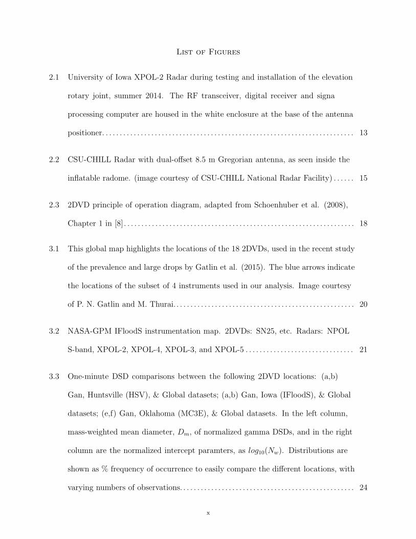
2.1 University of Iowa XPOL-2 Radar during testing and installation of the elevation

rotary joint, summer 2014. The RF transceiver, digital receiver and signa

processing computer are housed in the white enclosure at the base of the antenna

positioner. . . . . . . . . . . . . . . . . . . . . . . . . . . . . . . . . . . . . . . . . . . . . . . . . . . . . . . . . . . . . . . . . . . . . . . . 13

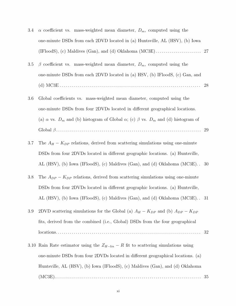
2.2 CSU-CHILL Radar with dual-offset 8.5 m Gregorian antenna, as seen inside the

inflatable radome. (image courtesy of CSU-CHILL National Radar Facility) . . . . . . 15

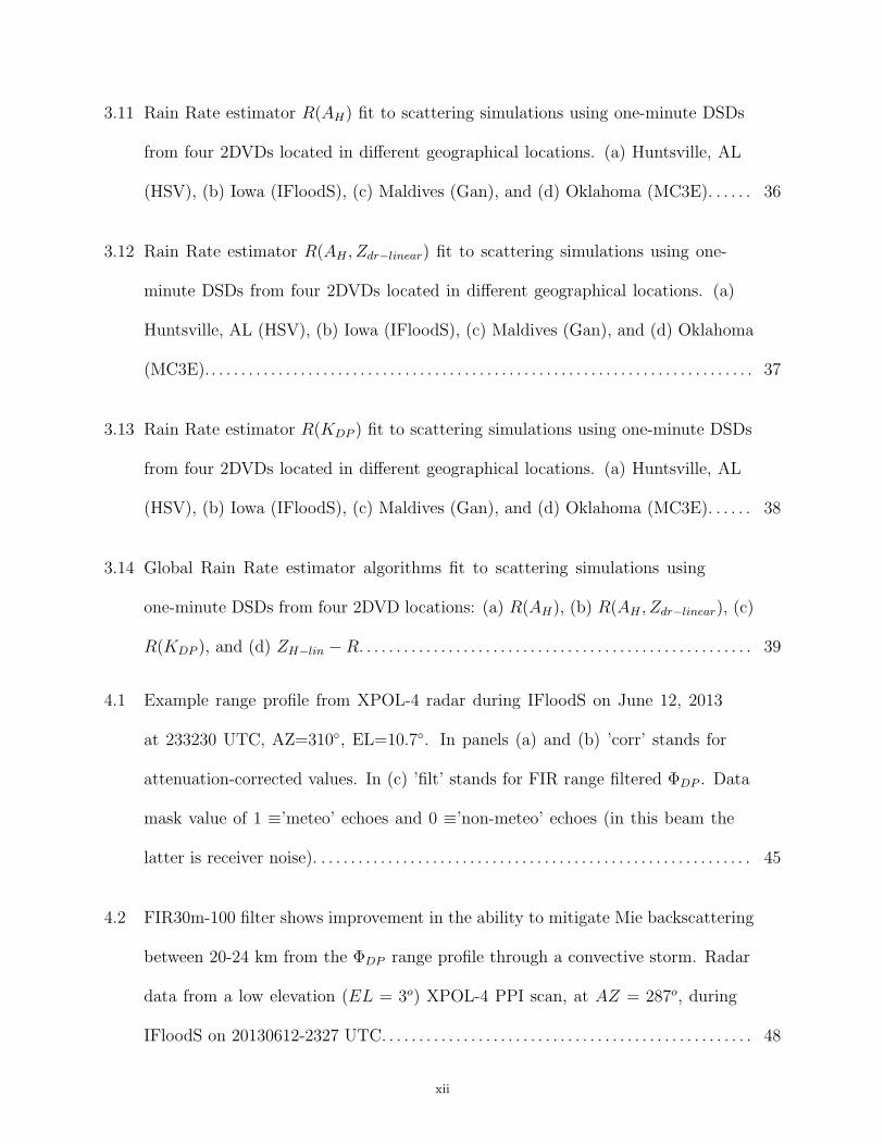
2.3 2DVD principle of operation diagram, adapted from Schoenhuber et al. (2008),

Chapter 1 in [8] . . . . . . . . . . . . . . . . . . . . . . . . . . . . . . . . . . . . . . . . . . . . . . . . . . . . . . . . . . . . . . . . . . 18

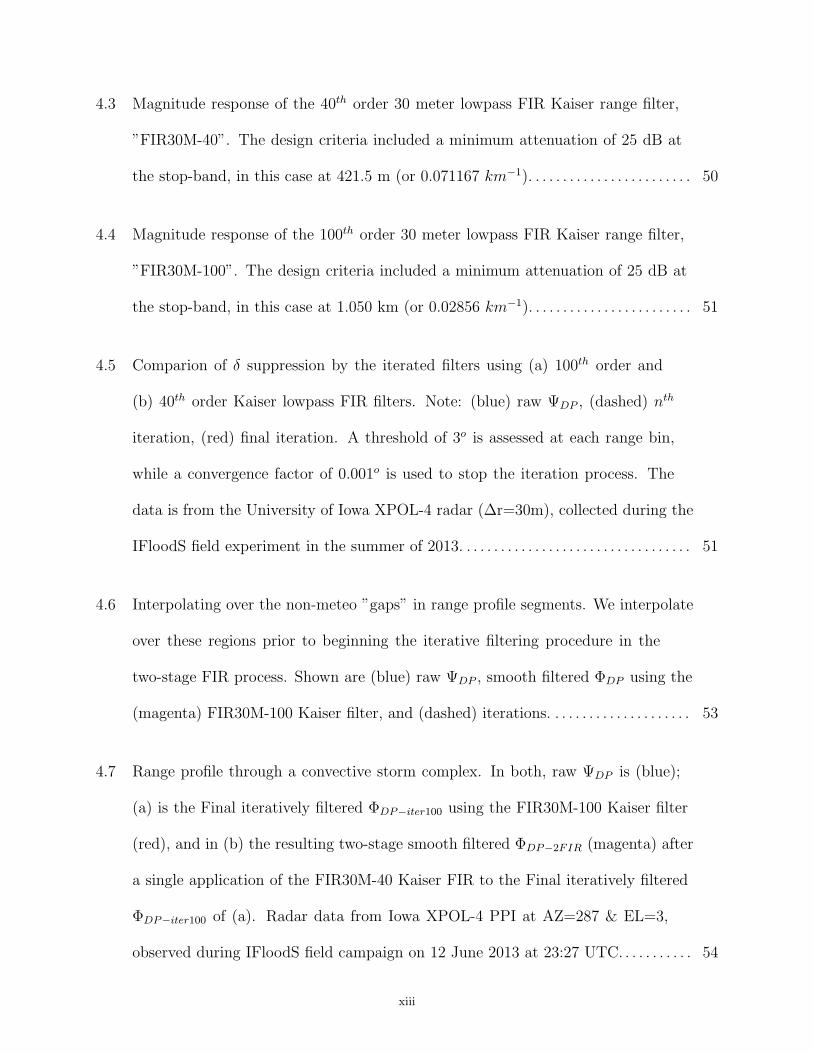
3.1 This global map highlights the locations of the 18 2DVDs, used in the recent study

of the prevalence and large drops by Gatlin et al. (2015). The blue arrows indicate

the locations of the subset of 4 instruments used in our analysis. Image courtesy

of P. N. Gatlin and M. Thurai. . . . . . . . . . . . . . . . . . . . . . . . . . . . . . . . . . . . . . . . . . . . . . . . . . . . 20

3.2 NASA-GPM IFloodS instrumentation map. 2DVDs: SN25, etc. Radars: NPOL

S-band, XPOL-2, XPOL-4, XPOL-3, and XPOL-5 . . . . . . . . . . . . . . . . . . . . . . . . . . . . . . . 21

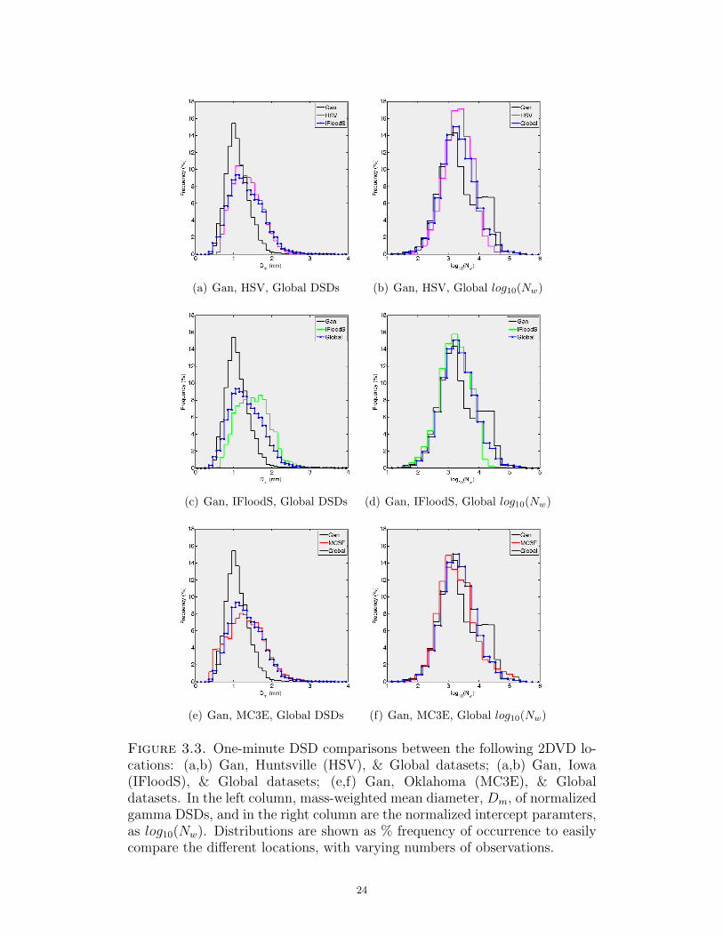
3.3 One-minute DSD comparisons between the following 2DVD locations: (a,b)

Gan, Huntsville (HSV), & Global datasets; (a,b) Gan, Iowa (IFloodS), & Global

datasets; (e,f) Gan, Oklahoma (MC3E), & Global datasets. In the left column,

mass-weighted mean diameter, Dm, of normalized gamma DSDs, and in the right

column are the normalized intercept paramters, as log10(Nw). Distributions are

shown as % frequency of occurrence to easily compare the different locations, with

varying numbers of observations. . . . . . . . . . . . . . . . . . . . . . . . . . . . . . . . . . . . . . . . . . . . . . . . . . 24

x

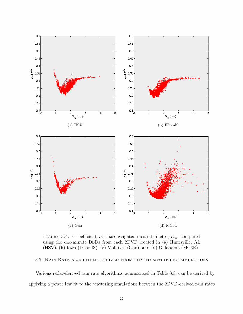
3.4 α coefficient vs. mass-weighted mean diameter, Dm, computed using the

one-minute DSDs from each 2DVD located in (a) Huntsville, AL (HSV), (b) Iowa

(IFloodS), (c) Maldives (Gan), and (d) Oklahoma (MC3E). . . . . . . . . . . . . . . . . . . . . . . 27

3.5 β coefficient vs. mass-weighted mean diameter, Dm, computed using the

one-minute DSDs from each 2DVD located in (a) HSV, (b) IFloodS, (c) Gan, and

(d) MC3E . . . . . . . . . . . . . . . . . . . . . . . . . . . . . . . . . . . . . . . . . . . . . . . . . . . . . . . . . . . . . . . . . . . . . . . 28

3.6 Global coefficients vs. mass-weighted mean diameter, computed using the

one-minute DSDs from four 2DVDs located in different geographical locations.

(a) α vs. Dm and (b) histogram of Global α; (c) β vs. Dm and (d) histogram of

Global β . . . . . . . . . . . . . . . . . . . . . . . . . . . . . . . . . . . . . . . . . . . . . . . . . . . . . . . . . . . . . . . . . . . . . . . . . 29

3.7 The AH −KDP relations, derived from scattering simulations using one-minute

DSDs from four 2DVDs located in different geographic locations. (a) Huntsville,

AL (HSV), (b) Iowa (IFloodS), (c) Maldives (Gan), and (d) Oklahoma (MC3E). . 30

3.8 The ADP −KDP relations, derived from scattering simulations using one-minute

DSDs from four 2DVDs located in different geographic locations. (a) Huntsville,

AL (HSV), (b) Iowa (IFloodS), (c) Maldives (Gan), and (d) Oklahoma (MC3E). . 31

3.9 2DVD scattering simulations for the Global (a) AH −KDP and (b) ADP −KDP

fits, derived from the combined (i.e., Global) DSDs from the four geographical

locations. . . . . . . . . . . . . . . . . . . . . . . . . . . . . . . . . . . . . . . . . . . . . . . . . . . . . . . . . . . . . . . . . . . . . . . . . 32

3.10 Rain Rate estimator using the ZH−lin − R fit to scattering simulations using

one-minute DSDs from four 2DVDs located in different geographical locations. (a)

Huntsville, AL (HSV), (b) Iowa (IFloodS), (c) Maldives (Gan), and (d) Oklahoma

(MC3E).. . . . . . . . . . . . . . . . . . . . . . . . . . . . . . . . . . . . . . . . . . . . . . . . . . . . . . . . . . . . . . . . . . . . . . . . . 35

xi

3.11 Rain Rate estimator R(AH) fit to scattering simulations using one-minute DSDs

from four 2DVDs located in different geographical locations. (a) Huntsville, AL

(HSV), (b) Iowa (IFloodS), (c) Maldives (Gan), and (d) Oklahoma (MC3E). . . . . . 36

3.12 Rain Rate estimator R(AH , Zdr−linear) fit to scattering simulations using one-

minute DSDs from four 2DVDs located in different geographical locations. (a)

Huntsville, AL (HSV), (b) Iowa (IFloodS), (c) Maldives (Gan), and (d) Oklahoma

(MC3E).. . . . . . . . . . . . . . . . . . . . . . . . . . . . . . . . . . . . . . . . . . . . . . . . . . . . . . . . . . . . . . . . . . . . . . . . . 37

3.13 Rain Rate estimator R(KDP ) fit to scattering simulations using one-minute DSDs

from four 2DVDs located in different geographical locations. (a) Huntsville, AL

(HSV), (b) Iowa (IFloodS), (c) Maldives (Gan), and (d) Oklahoma (MC3E). . . . . . 38

3.14 Global Rain Rate estimator algorithms fit to scattering simulations using

one-minute DSDs from four 2DVD locations: (a) R(AH), (b) R(AH , Zdr−linear), (c)

R(KDP ), and (d) ZH−lin −R. . . . . . . . . . . . . . . . . . . . . . . . . . . . . . . . . . . . . . . . . . . . . . . . . . . . . 39

4.1 Example range profile from XPOL-4 radar during IFloodS on June 12, 2013

at 233230 UTC, AZ=310◦, EL=10.7◦. In panels (a) and (b) ’corr’ stands for

attenuation-corrected values. In (c) ’filt’ stands for FIR range filtered ΦDP . Data

mask value of 1 ≡’meteo’ echoes and 0 ≡’non-meteo’ echoes (in this beam the

latter is receiver noise). . . . . . . . . . . . . . . . . . . . . . . . . . . . . . . . . . . . . . . . . . . . . . . . . . . . . . . . . . . 45

4.2 FIR30m-100 filter shows improvement in the ability to mitigate Mie backscattering

between 20-24 km from the ΦDP range profile through a convective storm. Radar

data from a low elevation (EL = 3o) XPOL-4 PPI scan, at AZ = 287o, during

IFloodS on 20130612-2327 UTC. . . . . . . . . . . . . . . . . . . . . . . . . . . . . . . . . . . . . . . . . . . . . . . . . . 48

xii

4.3 Magnitude response of the 40th order 30 meter lowpass FIR Kaiser range filter,

”FIR30M-40”. The design criteria included a minimum attenuation of 25 dB at

the stop-band, in this case at 421.5 m (or 0.071167 km−1). . . . . . . . . . . . . . . . . . . . . . . . 50

4.4 Magnitude response of the 100th order 30 meter lowpass FIR Kaiser range filter,

”FIR30M-100”. The design criteria included a minimum attenuation of 25 dB at

the stop-band, in this case at 1.050 km (or 0.02856 km−1). . . . . . . . . . . . . . . . . . . . . . . . 51

4.5 Comparion of δ suppression by the iterated filters using (a) 100th order and

(b) 40th order Kaiser lowpass FIR filters. Note: (blue) raw ΨDP , (dashed) nth

iteration, (red) final iteration. A threshold of 3o is assessed at each range bin,

while a convergence factor of 0.001o is used to stop the iteration process. The

data is from the University of Iowa XPOL-4 radar (∆r=30m), collected during the

IFloodS field experiment in the summer of 2013. . . . . . . . . . . . . . . . . . . . . . . . . . . . . . . . . . 51

4.6 Interpolating over the non-meteo ”gaps” in range profile segments. We interpolate

over these regions prior to beginning the iterative filtering procedure in the

two-stage FIR process. Shown are (blue) raw ΨDP , smooth filtered ΦDP using the

(magenta) FIR30M-100 Kaiser filter, and (dashed) iterations. . . . . . . . . . . . . . . . . . . . . 53

4.7 Range profile through a convective storm complex. In both, raw ΨDP is (blue);

(a) is the Final iteratively filtered ΦDP−iter100 using the FIR30M-100 Kaiser filter

(red), and in (b) the resulting two-stage smooth filtered ΦDP−2FIR (magenta) after

a single application of the FIR30M-40 Kaiser FIR to the Final iteratively filtered

ΦDP−iter100 of (a). Radar data from Iowa XPOL-4 PPI at AZ=287 & EL=3,

observed during IFloodS field campaign on 12 June 2013 at 23:27 UTC. . . . . . . . . . . 54

xiii

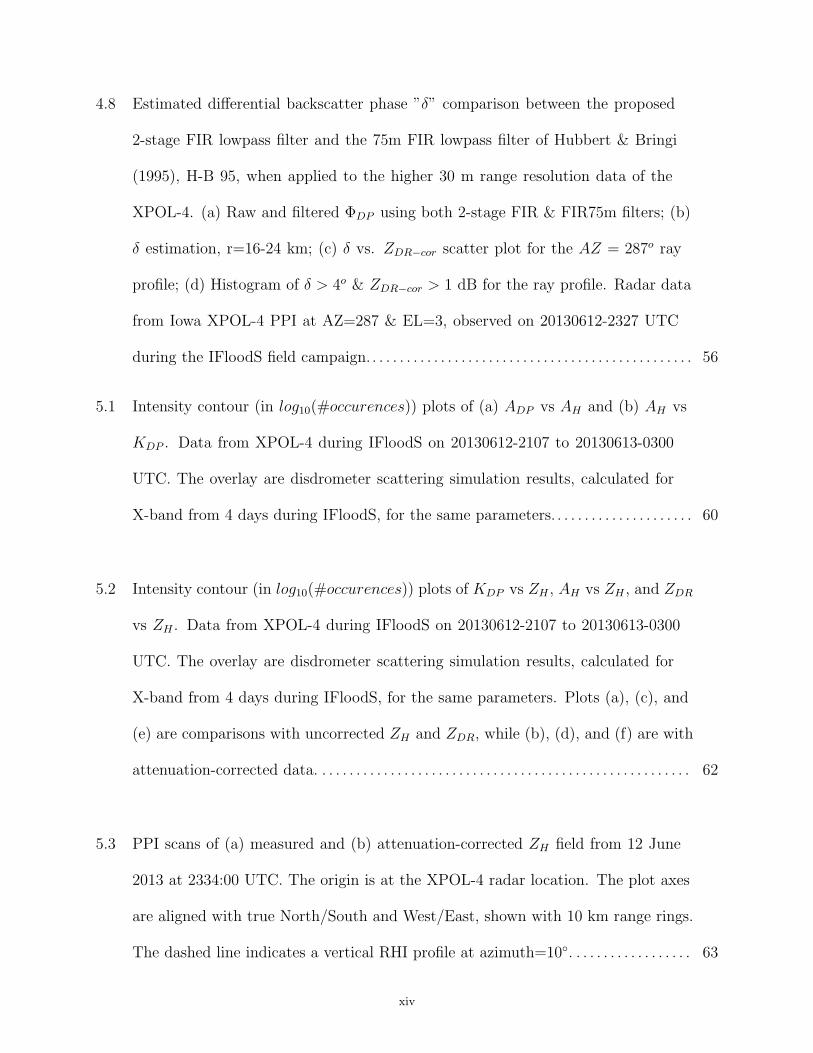
4.8 Estimated differential backscatter phase ”δ” comparison between the proposed

2-stage FIR lowpass filter and the 75m FIR lowpass filter of Hubbert & Bringi

(1995), H-B 95, when applied to the higher 30 m range resolution data of the

XPOL-4. (a) Raw and filtered ΦDP using both 2-stage FIR & FIR75m filters; (b)

δ estimation, r=16-24 km; (c) δ vs. ZDR−cor scatter plot for the AZ = 287o ray

profile; (d) Histogram of δ > 4o & ZDR−cor > 1 dB for the ray profile. Radar data

from Iowa XPOL-4 PPI at AZ=287 & EL=3, observed on 20130612-2327 UTC

during the IFloodS field campaign. . . . . . . . . . . . . . . . . . . . . . . . . . . . . . . . . . . . . . . . . . . . . . . . 56

5.1 Intensity contour (in log10(#occurences)) plots of (a) ADP vs AH and (b) AH vs

KDP . Data from XPOL-4 during IFloodS on 20130612-2107 to 20130613-0300

UTC. The overlay are disdrometer scattering simulation results, calculated for

X-band from 4 days during IFloodS, for the same parameters. . . . . . . . . . . . . . . . . . . . . 60

5.2 Intensity contour (in log10(#occurences)) plots of KDP vs ZH , AH vs ZH , and ZDR

vs ZH . Data from XPOL-4 during IFloodS on 20130612-2107 to 20130613-0300

UTC. The overlay are disdrometer scattering simulation results, calculated for

X-band from 4 days during IFloodS, for the same parameters. Plots (a), (c), and

(e) are comparisons with uncorrected ZH and ZDR, while (b), (d), and (f) are with

attenuation-corrected data. . . . . . . . . . . . . . . . . . . . . . . . . . . . . . . . . . . . . . . . . . . . . . . . . . . . . . . 62

5.3 PPI scans of (a) measured and (b) attenuation-corrected ZH field from 12 June

2013 at 2334:00 UTC. The origin is at the XPOL-4 radar location. The plot axes

are aligned with true North/South and West/East, shown with 10 km range rings.

The dashed line indicates a vertical RHI profile at azimuth=10◦. . . . . . . . . . . . . . . . . . 63

xiv

5.4 RHI scans of measured (panels (a) & (b)) and attenuation-corrected (panels (c) &

(d)) ZH and ZDR along the AZ=310◦, from XPOL-4 radar data during IFloodS

on June 12, 2013 at 2332:30 UTC, at AZ=310◦. The dashed line indicates the ray

profile at an EL=10.7◦ . . . . . . . . . . . . . . . . . . . . . . . . . . . . . . . . . . . . . . . . . . . . . . . . . . . . . . . . . . . 64

5.5 RHI scan of calculated KDP from XPOL-4 radar during IFloodS on June 12, 2013

at 2332:30 UTC, at AZ=310◦. The colorbar units are in deg/km, and the dashed

line indicates the EL=10.7◦ beam. . . . . . . . . . . . . . . . . . . . . . . . . . . . . . . . . . . . . . . . . . . . . . . . 65

5.6 XPOL-2 to XPOL-4 radar intercomparison during IFloodS on June 12, 2013 at

23:18 & 23:19 UTC, respectively. Upper panels in the left column show RHIs

from XPOL-2. (top) ZH−cor, (middle) ZDR−cor, (bottom) KDP . Agreement in the

attenuation-corrected values between the two radars is confirmed by congruency

in their respective distributions (right column) in the overlap region enclosed by a

6-20 km range interval and a 1-5 km height, marked by the box in the top panel.

Image adapted from [23] . . . . . . . . . . . . . . . . . . . . . . . . . . . . . . . . . . . . . . . . . . . . . . . . . . . . . . . . . 68

5.7 Advection is visible as rain falls to the right in this photo taken during a recent

Northern Colorado spring thunderstorm. When analyzing high resolution (30 m or

less) radar derived rain rates, this effect suggests we cannot only select range bins

directly above and adjacent to the rain gauges for comparison, but rather select

the nearest neighbor bins with minimal errors to in situ rain rates measured on

the ground. (Photo by M. B. Galvez, May 2, 2015). . . . . . . . . . . . . . . . . . . . . . . . . . . . . . . 69

5.8 XPOL-4 ZH−cor PPI plot of an inbound convective storm, highlighting the

locations of 12 NASA dual tipping rain gauges within its 40 km unambiguous

range. A blow-up is shown for Gauges 32 and 43, which are used to illustrate the

nearest-neighbor selection criteria for range bins within a radius rnn < 500m of

xv

the gauges. The �’s represent the starting azimuth of the range bin, and the ⋄’s

the center of the bin. Radar data from XPOL-4 during IFloodS on 20130612-2334

UTC. . . . . . . . . . . . . . . . . . . . . . . . . . . . . . . . . . . . . . . . . . . . . . . . . . . . . . . . . . . . . . . . . . . . . . . . . . . . . 71

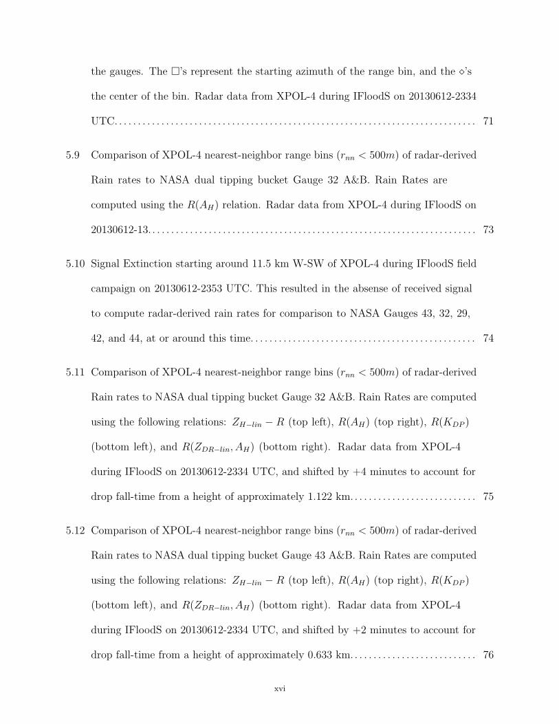
5.9 Comparison of XPOL-4 nearest-neighbor range bins (rnn < 500m) of radar-derived

Rain rates to NASA dual tipping bucket Gauge 32 A&B. Rain Rates are

computed using the R(AH) relation. Radar data from XPOL-4 during IFloodS on

20130612-13. . . . . . . . . . . . . . . . . . . . . . . . . . . . . . . . . . . . . . . . . . . . . . . . . . . . . . . . . . . . . . . . . . . . . . 73

5.10 Signal Extinction starting around 11.5 km W-SW of XPOL-4 during IFloodS field

campaign on 20130612-2353 UTC. This resulted in the absense of received signal

to compute radar-derived rain rates for comparison to NASA Gauges 43, 32, 29,

42, and 44, at or around this time. . . . . . . . . . . . . . . . . . . . . . . . . . . . . . . . . . . . . . . . . . . . . . . . 74

5.11 Comparison of XPOL-4 nearest-neighbor range bins (rnn < 500m) of radar-derived

Rain rates to NASA dual tipping bucket Gauge 32 A&B. Rain Rates are computed

using the following relations: ZH−lin − R (top left), R(AH) (top right), R(KDP )

(bottom left), and R(ZDR−lin, AH) (bottom right). Radar data from XPOL-4

during IFloodS on 20130612-2334 UTC, and shifted by +4 minutes to account for

drop fall-time from a height of approximately 1.122 km. . . . . . . . . . . . . . . . . . . . . . . . . . . 75

5.12 Comparison of XPOL-4 nearest-neighbor range bins (rnn < 500m) of radar-derived

Rain rates to NASA dual tipping bucket Gauge 43 A&B. Rain Rates are computed

using the following relations: ZH−lin − R (top left), R(AH) (top right), R(KDP )

(bottom left), and R(ZDR−lin, AH) (bottom right). Radar data from XPOL-4

during IFloodS on 20130612-2334 UTC, and shifted by +2 minutes to account for

drop fall-time from a height of approximately 0.633 km. . . . . . . . . . . . . . . . . . . . . . . . . . . 76

xvi

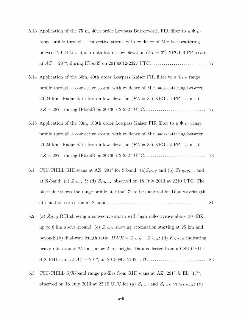
5.13 Application of the 75 m, 40th order Lowpass Butterworth FIR filter to a ΦDP

range profile through a convective storm, with evidence of Mie backscattering

between 20-24 km. Radar data from a low elevation (EL = 3o) XPOL-4 PPI scan,

at AZ = 287o, during IFloodS on 20130612-2327 UTC. . . . . . . . . . . . . . . . . . . . . . . . . . . . 77

5.14 Application of the 30m, 40th order Lowpass Kaiser FIR filter to a ΦDP range

profile through a convective storm, with evidence of Mie backscattering between

20-24 km. Radar data from a low elevation (EL = 3o) XPOL-4 PPI scan, at

AZ = 287o, during IFloodS on 20130612-2327 UTC. . . . . . . . . . . . . . . . . . . . . . . . . . . . . . 77

5.15 Application of the 30m, 100th order Lowpass Kaiser FIR filter to a ΦDP range

profile through a convective storm, with evidence of Mie backscattering between

20-24 km. Radar data from a low elevation (EL = 3o) XPOL-4 PPI scan, at

AZ = 287o, during IFloodS on 20130612-2327 UTC. . . . . . . . . . . . . . . . . . . . . . . . . . . . . . 78

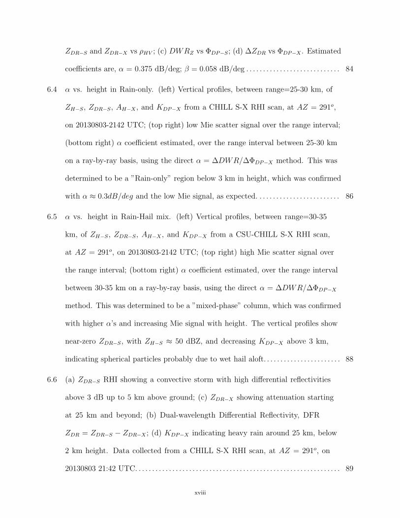
6.1 CSU-CHILL RHI scans at AZ=291◦ for S-band: (a)ZH−S and (b) ZDR−Ssm, and

at X-band: (c) ZH−X & (d) ZDR−X observed on 18 July 2013 at 2210 UTC. The

black line shows the range profile at EL=1.7◦ to be analyzed for Dual wavelength

attenuation correction at X-band. . . . . . . . . . . . . . . . . . . . . . . . . . . . . . . . . . . . . . . . . . . . . . . . . 81

6.2 (a) ZH−S RHI showing a convective storm with high reflectivities above 50 dBZ

up to 8 km above ground; (c) ZH−X showing attenuation starting at 25 km and

beyond; (b) dual-wavelength ratio, DWR = ZH−S − ZH−X ; (d) KDP−X indicating

heavy rain around 25 km, below 2 km height. Data collected from a CSU-CHILL

S-X RHI scan, at AZ = 291o, on 20130803-2142 UTC. . . . . . . . . . . . . . . . . . . . . . . . . . . . 83

6.3 CSU-CHILL S/X-band range profiles from RHI scans at AZ=291◦ & EL=1.7◦,

observed on 18 July 2013 at 22:10 UTC for (a) ZH−S and ZH−X vs ΦDP−X ; (b)

xvii

ZDR−S and ZDR−X vs ρHV ; (c) DWRZ vs ΦDP−S; (d) ∆ZDR vs ΦDP−X . Estimated

coefficients are, α = 0.375 dB/deg; β = 0.058 dB/deg . . . . . . . . . . . . . . . . . . . . . . . . . . . . 84

6.4 α vs. height in Rain-only. (left) Vertical profiles, between range=25-30 km, of

ZH−S, ZDR−S, AH−X , and KDP−X from a CHILL S-X RHI scan, at AZ = 291o,

on 20130803-2142 UTC; (top right) low Mie scatter signal over the range interval;

(bottom right) α coefficient estimated, over the range interval between 25-30 km

on a ray-by-ray basis, using the direct α = ∆DWR/∆ΦDP−X method. This was

determined to be a ”Rain-only” region below 3 km in height, which was confirmed

with α ≈ 0.3dB/deg and the low Mie signal, as expected. . . . . . . . . . . . . . . . . . . . . . . . . 86

6.5 α vs. height in Rain-Hail mix. (left) Vertical profiles, between range=30-35

km, of ZH−S, ZDR−S, AH−X , and KDP−X from a CSU-CHILL S-X RHI scan,

at AZ = 291o, on 20130803-2142 UTC; (top right) high Mie scatter signal over

the range interval; (bottom right) α coefficient estimated, over the range interval

between 30-35 km on a ray-by-ray basis, using the direct α = ∆DWR/∆ΦDP−X

method. This was determined to be a ”mixed-phase” column, which was confirmed

with higher α’s and increasing Mie signal with height. The vertical profiles show

near-zero ZDR−S, with ZH−S ≈ 50 dBZ, and decreasing KDP−X above 3 km,

indicating spherical particles probably due to wet hail aloft. . . . . . . . . . . . . . . . . . . . . . . 88

6.6 (a) ZDR−S RHI showing a convective storm with high differential reflectivities

above 3 dB up to 5 km above ground; (c) ZDR−X showing attenuation starting

at 25 km and beyond; (b) Dual-wavelength Differential Reflectivity, DFR

ZDR = ZDR−S − ZDR−X ; (d) KDP−X indicating heavy rain around 25 km, below

2 km height. Data collected from a CHILL S-X RHI scan, at AZ = 291o, on

20130803 21:42 UTC. . . . . . . . . . . . . . . . . . . . . . . . . . . . . . . . . . . . . . . . . . . . . . . . . . . . . . . . . . . . . 89

xviii

6.7 β vs. height in Rain-only. (left) Vertical profiles, between range=25-30 km, of

ZH−S, ZDR−S, ZDR−X , and KDP−X from a CHILL S-X RHI scan, at AZ = 291o, on

20130803-2142 UTC; (top right) 1dB < ∆ZDR < 3.5dB over the range interval and

below 2 km height; (bottom right) β coefficient estimated, over the range interval

between 25-30 km on a ray-by-ray basis, using the direct β = ∆ZDR/∆ΦDP−X

method. This was in a heavy ”Rain-only” region below 3 km in height, which was

confirmed with β ≈ 0.06dB/deg. . . . . . . . . . . . . . . . . . . . . . . . . . . . . . . . . . . . . . . . . . . . . . . . . . 91

6.8 Dual-wavelength derived α and β coeffients in Rain only. Radar data was collected

by CSU-CHILL S/X band radar on 20130803 at 21:42, 21:53, and 22:03 UTC.. . . . 92

6.9 Dual-wavelength derived α coeffient in Rain-Hail mixed phase. (a) Radar data was

collected by CSU-CHILL S/X band radar on 3 August 2013 at 21:42, 21:53, and

22:03 UTC. . . . . . . . . . . . . . . . . . . . . . . . . . . . . . . . . . . . . . . . . . . . . . . . . . . . . . . . . . . . . . . . . . . . . . . 93

xix

CHAPTER 1

Introduction

1.1. Motivation and Background

The backbone of weather monitoring, nowcasting and forecasting is the long range net-

work of S-band Doppler, dual-polarization radars such as NEXRAD in the US and C-band

counterparts in Europe, Japan and many other countires. The main driving force for dual-

polarization upgrade to the NEXRAD network was based on improvements in rain fall es-

timation, improved hail detection and improved data quality by virtue of distinguishing

between ’meteo’ and non-meteo echoes. In the past, single polarized X-band radars were

relegated to short range applications due to attenuation in moderate to severe weather.

However , in the last decade the atmospheric community has seen widespread and successful

application of X-band dual-polarization weather radars for measuring precipitation in the

lowest two km of the troposphere. These X-band radars have the advantage of a smaller foot-

print, lower cost, and improved detection of hydrometeors due to increased range resolution.

In recent years, the hydrology community began incorporating these radars in novel appli-

cations to study the spatio-temporal variability of rainfall from precipitation measurements

near the ground, over watersheds of interest. The University of Iowa XPOL radar system is

one of the first to be used as an X-band polarimetric radar network dedicated to hydrology

studies. During the spring of 2013, the Iowa XPOL radars participated in NASA Global

Precipitation Measurement (GPM) mission’s first field campaign focused solely on hydrology

studies, called the Iowa Flood Studies (IFloodS). A collaborative effort between Dr. Bringi’s

polarimetric radar lab at CSU and the Iowa Flood Center has led to the investigation of im-

provements upon the currently employed attenuation correction methods, with the intent of

1

obtaining more accurate radar-derived rain estimates for hydrological applications. X-band

dual-polarized radars are also being used extensively in networked configuration to monitor

severe weather events such as tornadic super cells (the network also provides for dual- or

multiple Doppler derived wind fields). Such compact networks are also being investigated as

gap-filler radars within the NEXRAD S-band network of long range radars covering the en-

tire US. Another application is hydrometeor-type classification whereby fuzzy logic methods

based on dual-polarized radar data are used to classify ’meteo’ versus ’non-meteo’ echoes

and further classify ’meteo’ echoes as due to rain, hail, snow etc. For all these applications,

attenuation-correction is a crucial step which is the main topic of this dissertation.

1.2. Problem Statement

Weather radars operating in the 3.2 cm (X-band) regime can suffer from severe atten-

uation, particularly during heavy convective storms. This has led to the development of

sophisticated algorithms for X-band radars to correct the meteorological observables for at-

tenuation. Although X-band polarimetric weather radars have seen increased acceptance

by the atmospheric and hydrology communities in recent years, the attenuation correction

aspect remains relatively unexamined. This research studies the problem of correcting for

precipitation-induced attenuation in X-band polarimetric weather radars with high spatio-

temporal resolution for hydrological applications. The research objectives of this dissertation

are focused in the following general areas:

I. The first objective is to understand the role regional climatology has on the variability

of 2DVD scattering simulations from a drop size distribution viewpoint, as well as

its effects on the α and β coefficients, and lastly on derived rain rate algorithms, as

compared to that derived from a global climatology.

2

II. The second objective is to investigate the ZPHI method for attenuation correction

of precipitation-induced attenuation in X-band polarimetric radars with high spatio-

temporal resolution dedicated to hydrology studies of vast river basins and water-

sheds. We also study the effects of filtering techniques used to estimate the differential

backscatter phase due to Mie scattering effects at X-band.

III. The third objective is to evaluate performance of the attenuation correction and FIR

filtering algorithms, applied to the high spatio-temporal data collected by the Univer-

sity of Iowa XPOL radars, during the hydrology-focused NASA-GPM mission, Iowa

Flood Studies (or IFloodS) field campaign conducted in the spring of 2013.

IV. For the final objective, we investigate dual-wavelength algorithms to directly estimate

the α and β coefficients, of the AH = αKDP and ADP = βKDP relations, to obtain

the path integrated attenuation due to rain and wet ice or snow in the region near the

melting layer. We analyze data from the dual-wavelength, dual-polarization CHILL

S-/X-band Doppler weather radar to examine the coefficients and compare their vari-

ability as a function of height, where the hydrometeors are expected to go through a

microphysical transformation as they fall, starting as snow or graupel/hail then melting

into rain or a rain-hail mixture.

3

CHAPTER 2

Theoretical Background and Instrumentation

In this chapter, theoretical background is presented to introduce important concepts

specific to dual-polarized (i.e., polarimetric) radar, like the weather radar equation and the

backscatter of electromagnetic waves from precipitation. The backscatter cross-section is

discussed with respect to the dielectric factor for water and ice, where it is dependent on

wavelength and temperature. The backscatter cross-section is related to the radar reflectiv-

ity factor (i.e., ZH,V ) from horizontal and vertical polarizations, from which their difference

provides detail about the drop shape, as the differential reflectivity, ZDR. The absorption

and scattering cross sections combined make up the extinction cross section, from which

the specific attenuation in horizontal polarization, AH , can be derived. The specific dif-

ferential phase, KDP , is also presented, as is the co-polar differential phase, from which

we will derive several relations for attenuation correction procedures and radar-derived rain

rate algorithms. Also included in this chapter is background related to dual-wavelength

ratios (DWR) for reflectivity and differential reflectivity, that allow for direct derivation of

attenuation correction coefficients (α & β), from differences in measured S-band to X-band

wavelength radar moments.

We present the various key instruments used to investigate attenuation correction meth-

ods for X-band polarimetric radars with high spatio-temporal resolution, like the Univer-

sity of Iowa XPOL mobile radar platform, and the CSU-CHILL dual-wavelength dual-

polarization weather radar (operating at both S- & X-bands). The two-dimensional video

disdrometer, used to make in situ measurements of drop size distributions near to the ground

is introduced, along with some key computations in estimating the rain rates and drop sizes

4

within the distribution measured. In essence, this chapter introduces the theoretical back-

ground and key instrumentation used to realize this research.

2.1. Dual-polarized Radar

2.1.1. The Weather Radar Equation. The weather radar equation is a volumetric

estimation of scattering from hydrometeors, rather than a point target equation. Here we

estimate the effective reflectivity based on the drop size distribution (DSD) in a volume

defined by the horizontal and vertical beam widths, as well as the radial range gate spacing.

Reflectivity, η, is the general radar term describing the volumetric backscatter cross-

section per unit volume, and is calculated from the received complex signal envelope, derived

from the discrete I + jQ components at the output of the digital receiver. The reflectivity

from meteorological backscatterers can be written as, η = (π5/λ4)|kw|2Ze. The equivalent

reflectivity factor Ze can be estimated from the received power, Pr, using the weather radar

equation [1], shown here in a form for units commonly used by radar meteorologists,

(2.1) Pr =π510−17PtG

2Grτθ2

3dB|kw|2Ze

6.75x214 ln2 r2λ2l2lr

Receive power at range r, P (r) is measured in mW , transmit power Pt in Watts, antenna

and receiver gains, G and Gr are dimensionless, transmit pulse width τ in micro seconds

(µs), antenna 3dB-beamwidth (H and V) θ3dB in degrees, the dielectric factor of water

|kw|2 = |(ǫr − 1)/(ǫr + 2)|2 where ǫr is the complex relative permittivity of water, the range

r is in kilometers, wavelength λ is in centimeters, and attenuation and receiver losses, l and

lr are dimensionless. The equivalent reflectivity factor Ze is simply referred to, by radar

meteorologists, as reflectivity for H,V polarizations at a range r, Zh,v(r) measured in units

of mm6m−3 in dBZ.

5

By rearranging the weather radar equation the reflectivity, at range r, for a given power

measured at the H and V channel outputs of the digital receiver, can be expressed as,

(2.2) Zh,v(r) =

(

6.75x214 ln2

π510−17

)(

lr G2

τ θ23dB |kw|2

)(

λ2(fNCO) l2

Pt Gr(fNCO)

)

r2 Ph,v(r)

where the quantities within the parentheses represent parts of the radar system constant

C = CkCsCd, Ck is a numerical constant, Cs is dependent on static system hardware param-

eters including the antenna and receiver gains, and Cd is dependent on dynamic hardware

parameters such as sampled transmit frequency and associated automatic frequency control

parameters (i.e., fNCO) set during the coherent-on-receive step. For example, the transmit-

ted wavelength perturbations are due to the random variations in frequency output from the

magnetron, and calculated as λ(fNCO) = c/(fNCO + fSTALO), where the STALO frequency

is fixed, and the NCO frequency varies depending on the estimated frequency of the sampled

transmit pulse. It is widely accepted in the radar meteorology community to represent Z

using a logarithmic scale and written as,

(2.3) Zh,v(r) = 10 log[ C Ph,v(r) r2] [in dBZ]

and will henceforth be referred to in dBZ. The noise in a radar system is an important

factor to keep track of, and so the radar equation can be rewritten as a signal-to-noise ratio

(SNR) by dividing through by the noise power resulting in,

(2.4) SNR =PR

NR

=λPTG

2σ

(4π)3R4L(kTFN)B

6

where k is the Boltzmann’s constant = 1.38 x 10−23J/K, T is the nominal noise temperature

(290K), FN is the receiver system noise factor, B is the bandwidth at the antenna port, and

L are the losses within the transmitter and receiver systems.

2.1.2. Backscatter of electromagnetic waves. The radar equation is based on

the physics of electromagnetic propagation out from and returning to the antenna. The

returning electromagnetic energy emitted by the scatterers (e.g., hydrometeors like rain

drops, hail, snow, etc.) is commonly referred to as backscatter which has a radar cross

section, σ = 4πR2 limR→∞(Pr

Pi

), the limit of the ratio of received power to incident power as

the range approaches infinity. There are three regions of scattering relating the radius a of a

spherical backscatterer to the operating wavelength λ which are: Rayleigh, Mie or resonant,

and the optical regions. The Rayleigh scattering region includes a ≪ λ (approximately

D < λ/16), while the optical region is for a ≫ λ. Between these two, the Mie solution to

Maxwell’s equations is applied.

Assuming the particle lies in the Rayleigh region, the backscattering cross section can be

approximated by,

(2.5) σb =π5|kw|2D6

λ4

where D = 2a, and |kw|2 = |(ǫr − 1)/(ǫr +2)|2, is the dielectric factor for water and ǫr is the

complex relative permitivity of the dielectric and can be expressed ǫr = ǫ′

+ iǫ” (complex

dielectric constant that is time dependent as e−jωt ). The real part of ǫr is the relative

permittivity, while the imaginary part is the loss factor associated with wave attenuation.

The dielectric factor kw depends on the wavelength and temperature, where for example

7

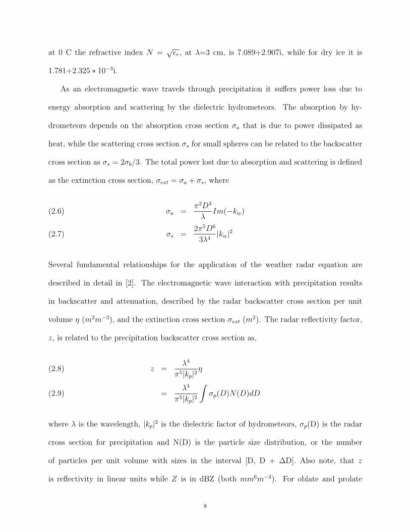
at 0 C the refractive index N =√ǫr, at λ=3 cm, is 7.089+2.907i, while for dry ice it is

1.781+2.325 ∗ 10−3i.

As an electromagnetic wave travels through precipitation it suffers power loss due to

energy absorption and scattering by the dielectric hydrometeors. The absorption by hy-

drometeors depends on the absorption cross section σa that is due to power dissipated as

heat, while the scattering cross section σs for small spheres can be related to the backscatter

cross section as σs = 2σb/3. The total power lost due to absorption and scattering is defined

as the extinction cross section, σext = σa + σs, where

σa =π2D3

λIm(−kw)(2.6)

σs =2π5D6

3λ4|kw|2(2.7)

Several fundamental relationships for the application of the weather radar equation are

described in detail in [2]. The electromagnetic wave interaction with precipitation results

in backscatter and attenuation, described by the radar backscatter cross section per unit

volume η (m2m−3), and the extinction cross section σext (m2). The radar reflectivity factor,

z, is related to the precipitation backscatter cross section as,

z =λ4

π5|kp|2η(2.8)

=λ4

π5|kp|2∫

σp(D)N(D)dD(2.9)

where λ is the wavelength, |kp|2 is the dielectric factor of hydrometeors, σp(D) is the radar

cross section for precipitation and N(D) is the particle size distribution, or the number

of particles per unit volume with sizes in the interval [D, D + ∆D]. Also note, that z

is reflectivity in linear units while Z is in dBZ (both mm6m−3). For oblate and prolate

8

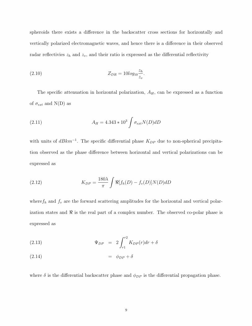
spheroids there exists a difference in the backscatter cross sections for horizontally and

vertically polarized electromagnetic waves, and hence there is a difference in their observed

radar reflectivies zh and zv, and their ratio is expressed as the differential reflectivity

(2.10) ZDR = 10log10zhzv.

The specific attenuation in horizontal polarization, AH , can be expressed as a function

of σext and N(D) as

(2.11) AH = 4.343 ∗ 103∫

σextN(D)dD

with units of dBkm−1. The specific differential phase KDP due to non-spherical precipita-

tion observed as the phase difference between horizontal and vertical polarizations can be

expressed as

(2.12) KDP =180λ

π

∫

ℜ[fh(D)− fv(D)]N(D)dD

wherefh and fv are the forward scattering amplitudes for the horizontal and vertical polar-

ization states and ℜ is the real part of a complex number. The observed co-polar phase is

expressed as

ΨDP = 2

∫ r2

r1

KDP (r)dr + δ(2.13)

= φDP + δ(2.14)

where δ is the differential backscatter phase and φDP is the differential propagation phase.

9

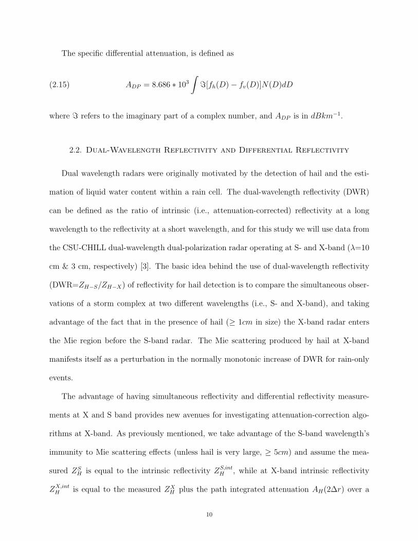
The specific differential attenuation, is defined as

(2.15) ADP = 8.686 ∗ 103∫

ℑ[fh(D)− fv(D)]N(D)dD

where ℑ refers to the imaginary part of a complex number, and ADP is in dBkm−1.

2.2. Dual-Wavelength Reflectivity and Differential Reflectivity

Dual wavelength radars were originally motivated by the detection of hail and the esti-

mation of liquid water content within a rain cell. The dual-wavelength reflectivity (DWR)

can be defined as the ratio of intrinsic (i.e., attenuation-corrected) reflectivity at a long

wavelength to the reflectivity at a short wavelength, and for this study we will use data from

the CSU-CHILL dual-wavelength dual-polarization radar operating at S- and X-band (λ=10

cm & 3 cm, respectively) [3]. The basic idea behind the use of dual-wavelength reflectivity

(DWR=ZH−S/ZH−X) of reflectivity for hail detection is to compare the simultaneous obser-

vations of a storm complex at two different wavelengths (i.e., S- and X-band), and taking

advantage of the fact that in the presence of hail (≥ 1cm in size) the X-band radar enters

the Mie region before the S-band radar. The Mie scattering produced by hail at X-band

manifests itself as a perturbation in the normally monotonic increase of DWR for rain-only

events.

The advantage of having simultaneous reflectivity and differential reflectivity measure-

ments at X and S band provides new avenues for investigating attenuation-correction algo-

rithms at X-band. As previously mentioned, we take advantage of the S-band wavelength’s

immunity to Mie scattering effects (unless hail is very large, ≥ 5cm) and assume the mea-

sured ZSH is equal to the intrinsic reflectivity ZS,int

H , while at X-band intrinsic reflectivity

ZX,intH is equal to the measured ZX

H plus the path integrated attenuation AH(2∆r) over a

10

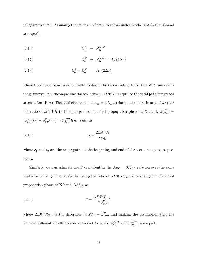
range interval ∆r. Assuming the intrinsic reflectivities from uniform echoes at S- and X-band

are equal,

ZSH = ZS,int

H(2.16)

ZXH = ZX,int

H − AH(2∆r)(2.17)

ZSH − ZX

H = AH(2∆r)(2.18)

where the difference in measured reflectivites of the two wavelengths is the DWR, and over a

range interval ∆r, encompassing ’meteo’ echoes, ∆DWR is equal to the total path integrated

attenuation (PIA). The coefficient α of the AH = αKDP relation can be estimated if we take

the ratio of ∆DWR to the change in differential propagation phase at X-band, ∆φXDP =

(φXDP (r0)− φX

DP (r1)) = 2∫ r0

r1KDP (s)ds, as

(2.19) α =∆DWR

∆φXDP

where r1 and r0 are the range gates at the beginning and end of the storm complex, respec-

tively.

Similarly, we can estimate the β coefficient in the ADP = βKDP relation over the same

’meteo’ echo range interval ∆r, by taking the ratio of ∆DWRZdr to the change in differential

propagation phase at X-band ∆φXDP , as

(2.20) β =∆DWRZdr

∆φXDP

where ∆DWRZdr is the difference in ZSDR − ZX

DR, and making the assumption that the

intrinsic differential reflectivities at S- and X-bands, ZS,intDR and ZX,int

DR , are equal.

11

2.3. Radar Platforms

During the course of this research, data from two different radar platforms are used.

These platforms are both transportable Doppler weather radars, although with contrasting

size scales, in particular: the first is a trailer-mounted radar node operating at X-band that

can be readily configured into a network; and the second is at a national facility as a stand

alone dual-wavelength, dual-polarization research radar operating at the S- and X-bands.

Specifications and a brief description about each system are presented in the subsequent

sections.

2.3.1. University of Iowa XPOL Radar System. The University of Iowa procured

four X-band polarimetric Doppler weather radars (XPOL) to more accurately estimate rain-

fall at high spatio-temporal resolution [4, 5]. The XPOL radar node is a compact, trans-

portable (i.e., trailer mounted), relatively low cost dual-polarization weather radar based on

a modified marine radar, seen here in Figure 2.1. The four XPOLs were identically designed

and manufactured by ProSensing, Inc., to the specifications listed in Table 2.1.

The XPOL radars can be set up to operate independently or in a complimentary net-

worked environment, in various configurations (i.e., with 2, 3, or 4 nodes), to simultaneously

observe rainfall near the ground, over a particular watershed of interest. Unlike most X-band

polarimetric radar networks that are typically tower mounted at fixed locations, the trans-

portability of the XPOL radar network allows for hydrological experiments of watersheds

located in more diverse locations, that normally might not be studied. The Iowa polarimetric

radar network was developed to serve the US hydrologic community to provide unique op-

portunities for hydrological studies requiring high spatio-temporal resolution, typically over

a network of rain gauges and disdrometers for comparative analyses.

12

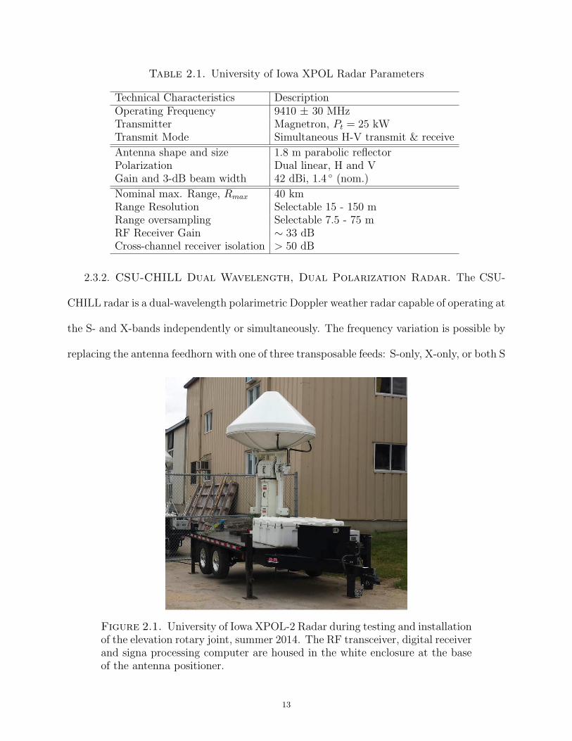
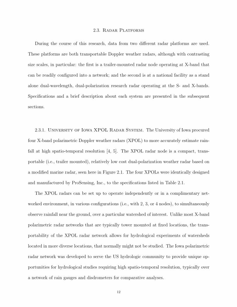
Table 2.1. University of Iowa XPOL Radar Parameters

Technical Characteristics DescriptionOperating Frequency 9410 ± 30 MHzTransmitter Magnetron, Pt = 25 kWTransmit Mode Simultaneous H-V transmit & receive

Antenna shape and size 1.8 m parabolic reflectorPolarization Dual linear, H and VGain and 3-dB beam width 42 dBi, 1.4 ◦ (nom.)

Nominal max. Range, Rmax 40 kmRange Resolution Selectable 15 - 150 mRange oversampling Selectable 7.5 - 75 mRF Receiver Gain ∼ 33 dBCross-channel receiver isolation > 50 dB

2.3.2. CSU-CHILL Dual Wavelength, Dual Polarization Radar. The CSU-

CHILL radar is a dual-wavelength polarimetric Doppler weather radar capable of operating at

the S- and X-bands independently or simultaneously. The frequency variation is possible by

replacing the antenna feedhorn with one of three transposable feeds: S-only, X-only, or both S

Figure 2.1. University of Iowa XPOL-2 Radar during testing and installationof the elevation rotary joint, summer 2014. The RF transceiver, digital receiverand signa processing computer are housed in the white enclosure at the baseof the antenna positioner.

13

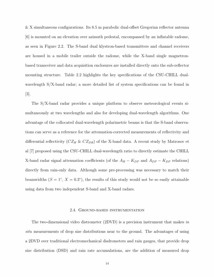
& X simultaneous configurations. Its 8.5 m parabolic dual-offset Gregorian reflector antenna

[6] is mounted on an elevation over azimuth pedestal, encompassed by an inflatable radome,

as seen in Figure 2.2. The S-band dual klystron-based transmitters and channel receivers

are housed in a mobile trailer outside the radome, while the X-band single magnetron-

based transceiver and data acquisition enclosures are installed directly onto the sub-reflector

mounting structure. Table 2.2 highlights the key specifications of the CSU-CHILL dual-

wavelength S/X-band radar; a more detailed list of system specifications can be found in

[3].

The S/X-band radar provides a unique platform to observe meteorological events si-

multaneously at two wavelengths and also for developing dual-wavelength algorithms. One

advantage of the collocated dual-wavelength polarimetric beams is that the S-band observa-

tions can serve as a reference for the attenuation-corrected measurements of reflectivity and

differential reflectivity (CZH & CZDR) of the X-band data. A recent study by Matrosov et

al [7] proposed using the CSU-CHILL dual-wavelength ratio to directly estimate the CHILL

X-band radar signal attenuation coefficients (of the AH −KDP and ADP −KDP relations)

directly from rain-only data. Although some pre-processing was necessary to match their

beamwidths (S = 1◦, X = 0.3◦), the results of this study would not be so easily attainable

using data from two independent S-band and X-band radars.

2.4. Ground-based instrumentation

The two-dimensional video distrometer (2DVD) is a precision instrument that makes in

situ measurements of drop size distributions near to the ground. The advantages of using

a 2DVD over traditional electromechanical disdrometers and rain gauges, that provide drop

size distribution (DSD) and rain rate accumulations, are the addition of measured drop

14

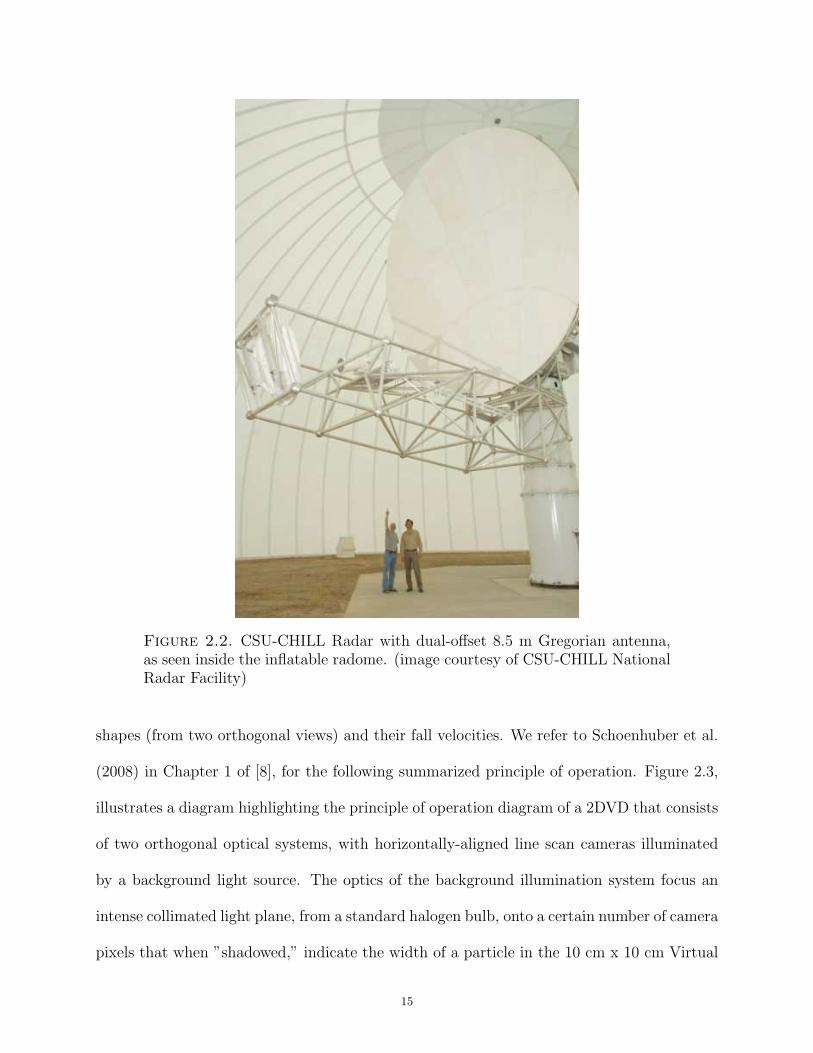
Figure 2.2. CSU-CHILL Radar with dual-offset 8.5 m Gregorian antenna,as seen inside the inflatable radome. (image courtesy of CSU-CHILL NationalRadar Facility)

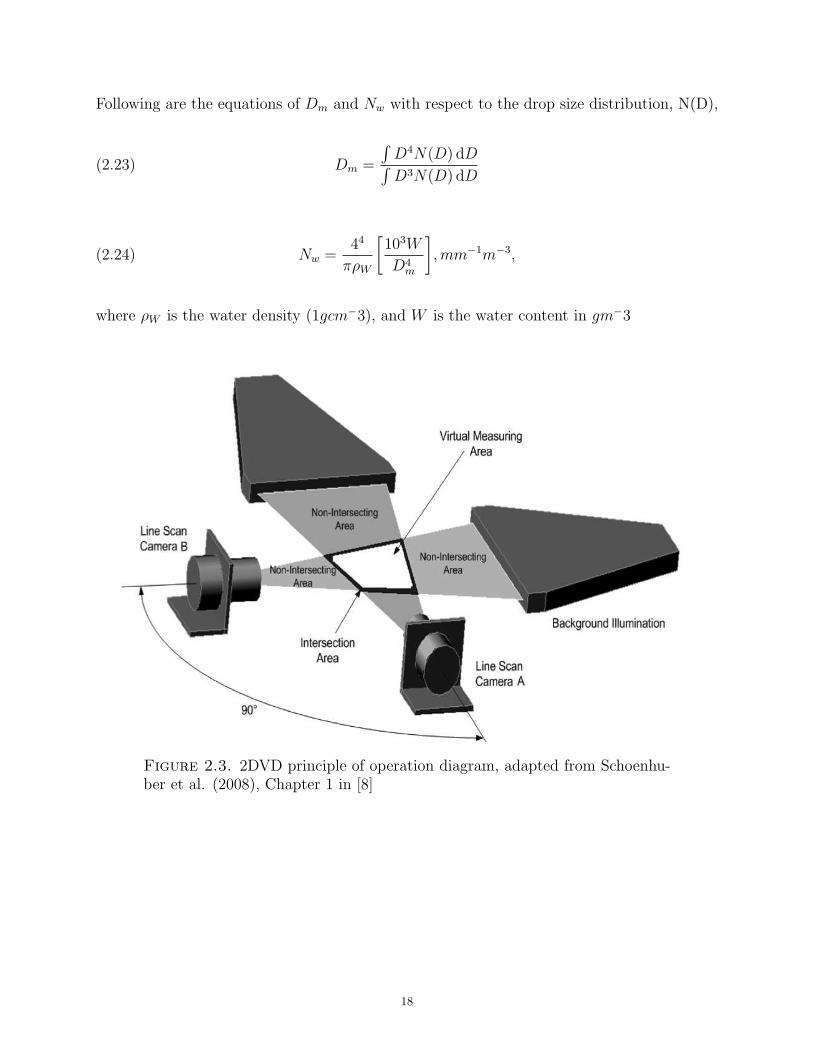
shapes (from two orthogonal views) and their fall velocities. We refer to Schoenhuber et al.

(2008) in Chapter 1 of [8], for the following summarized principle of operation. Figure 2.3,

illustrates a diagram highlighting the principle of operation diagram of a 2DVD that consists

of two orthogonal optical systems, with horizontally-aligned line scan cameras illuminated

by a background light source. The optics of the background illumination system focus an

intense collimated light plane, from a standard halogen bulb, onto a certain number of camera

pixels that when ”shadowed,” indicate the width of a particle in the 10 cm x 10 cm Virtual

15

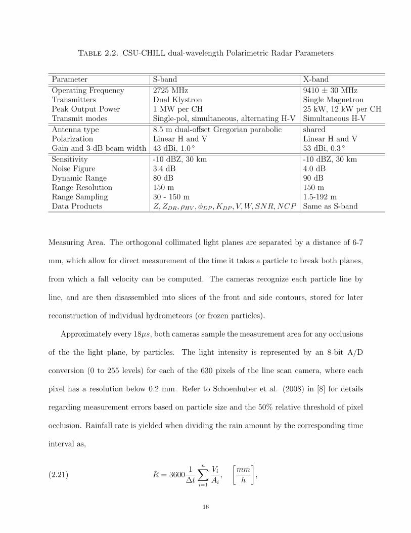
Table 2.2. CSU-CHILL dual-wavelength Polarimetric Radar Parameters

Parameter S-band X-band

Operating Frequency 2725 MHz 9410 ± 30 MHzTransmitters Dual Klystron Single MagnetronPeak Output Power 1 MW per CH 25 kW, 12 kW per CHTransmit modes Single-pol, simultaneous, alternating H-V Simultaneous H-V

Antenna type 8.5 m dual-offset Gregorian parabolic sharedPolarization Linear H and V Linear H and VGain and 3-dB beam width 43 dBi, 1.0 ◦ 53 dBi, 0.3 ◦

Sensitivity -10 dBZ, 30 km -10 dBZ, 30 kmNoise Figure 3.4 dB 4.0 dBDynamic Range 80 dB 90 dBRange Resolution 150 m 150 mRange Sampling 30 - 150 m 1.5-192 mData Products Z,ZDR, ρHV , φDP , KDP , V,W, SNR,NCP Same as S-band

Measuring Area. The orthogonal collimated light planes are separated by a distance of 6-7

mm, which allow for direct measurement of the time it takes a particle to break both planes,

from which a fall velocity can be computed. The cameras recognize each particle line by

line, and are then disassembled into slices of the front and side contours, stored for later

reconstruction of individual hydrometeors (or frozen particles).

Approximately every 18µs, both cameras sample the measurement area for any occlusions

of the the light plane, by particles. The light intensity is represented by an 8-bit A/D

conversion (0 to 255 levels) for each of the 630 pixels of the line scan camera, where each

pixel has a resolution below 0.2 mm. Refer to Schoenhuber et al. (2008) in [8] for details

regarding measurement errors based on particle size and the 50% relative threshold of pixel

occlusion. Rainfall rate is yielded when dividing the rain amount by the corresponding time

interval as,

(2.21) R = 36001

∆t

n∑

i=1

Vi

Ai

,

[

mm

h

]

,

16

where ∆t is the user-selectable integration time interval [> 15s], i is drop number, n is the

total number of fully visible drops measured in time interval ∆t, Vi is the volume of ith

drop [mm3], and Ai is the effective measuring area for the ith drop [mm2]. The DSDs are

calculated using information of the equivolume sphere diameter of raindrops, time stamps,

sizes of their effective measuring areas, their fall velocities, user-defined integration interval

and size class width. The DSD is the number of drops per unit volume per unit size, where

a particular size class is determined as,

(2.22) N(Di) =1

∆t∆D

mi∑

j=1

1

Ajvj,

[

1

m3mm

]

,

where ∆t is the user-selectable integration time interval [> 15s], i denotes a particular drop

size class, j denotes particular drop within size class i and time interval ∆t, mi is the number

of drops within size class i and time interval ∆t, Di is the mean diameter of class i [mm], ∆D

the width of drop size class [typically 0.25 mm], Aj is the effective measuring area for the jth

drop [m2], and finally vi the fall velocity of the jth drop [m/s]. For a more detailed overview

of the 2DVD, refer to [8, 9]. There are at least two important parameters that describe the

N(D). First is the mass-weighted mean drop diameter (Dm) defined as the ratio of the 4th to

3rd moments of the N(D). The second is the normalized intercept parameter (Nw) defined

(excluding constants) as the ratio of the rain water content to D4m. These two parameters

(Dm and Nw) can be defined for any measured N(D). The Nw is the same as the intercept

parameter (No) of an equivalent exponentially-shaped distribution that has the same Dm

and rain water content as the measured N(D). Note that the Marshall-Palmer exponential

DSD keeps N0=8,000 mm−1m−3 with Dm being expressed as a power law with rain rate, R.

17

Following are the equations of Dm and Nw with respect to the drop size distribution, N(D),

(2.23) Dm =

∫

D4N(D) dD∫

D3N(D) dD

(2.24) Nw =44

πρW

[

103W

D4m

]

,mm−1m−3,

where ρW is the water density (1gcm−3), and W is the water content in gm−3

Figure 2.3. 2DVD principle of operation diagram, adapted from Schoenhu-ber et al. (2008), Chapter 1 in [8]

18

CHAPTER 3

2-D Video Disdrometer (2DVD) Scattering

Simulations at X-band

3.1. Overview of the T-matrix Method

The transition, or T-matrix method is a numerical technique for calculating the scattering

from spheriods, first developed by [10], also referred to as the extended boundary condition

method. We summarize the description of the T-matrix, and defer details of the vector

spherical harmonic analysis and solution for the transition matrix presented in the appendices

(2,3,4) of the book Polarimetric Doppler Weather Radar: Principles and applications, by

Bringi and Chandrasekar (2001). In essence, a plane wave that is incident on the particle is

expanded in vector spherical harmonics (like a Fourier series) with known coefficients of the

plane wave, while the scattered field can also be expanded in vector spherical harmonics, with

unknown coefficients. The scattering coefficients and the incident plane wave coefficients are

relatable by the T-matrix, and dependent on the shape of the particle and its dielectric

constant, whereby we can determine the unknown scattering coefficients and incidentally

the backscattered field.

3.2. Use of global 2DVD scattering simulations to estimate a range of α &

β coefficients for X-band attenuation correction procedure

The data used for the scattering calculations is a subset of the global 2DVD datasets

used for a recent study on the prevalence and occurrence of large drops by [11]. The dataset

compiled consisted of a large and diverse set of measurements from 18 locations around the

globe. A map of these locations is given in Figures 3.1. Indicated on it with blue arrows are

19

four locations used in the current simulations, namely, (i) Huntsville, Alabama, (ii) Iowa,

(iii) Oklahoma, and (iv) Gan near Maldives. The first three are continental US locations

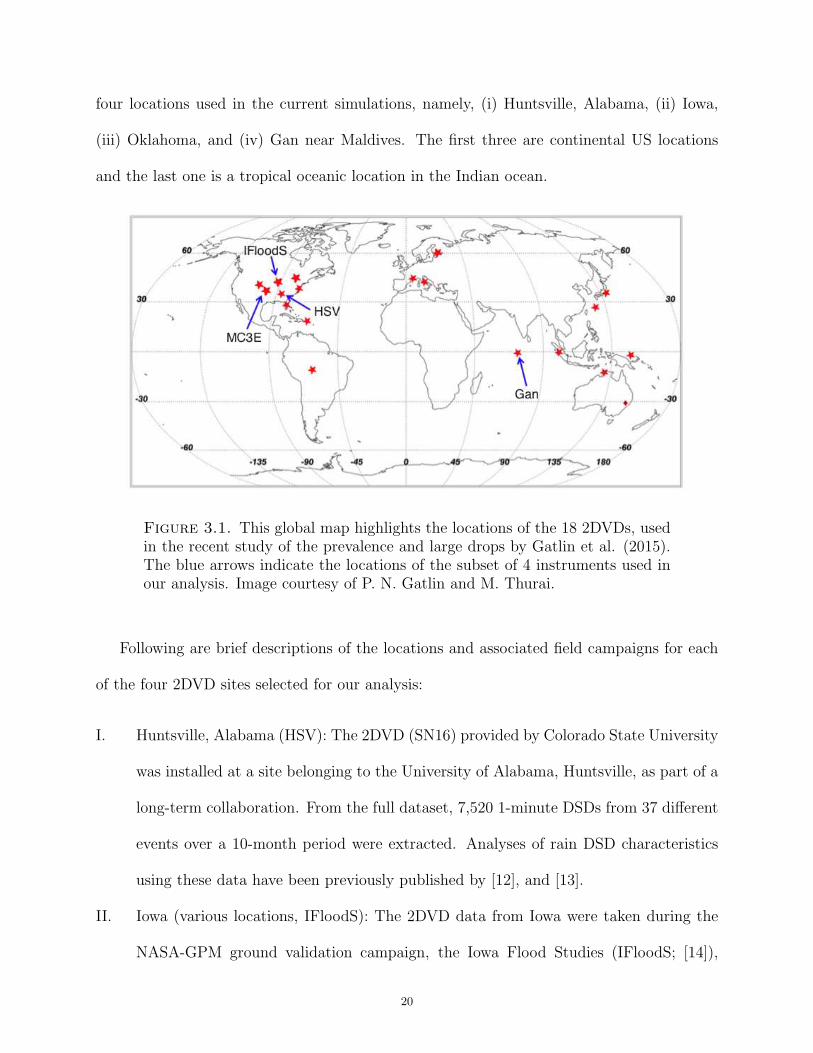
and the last one is a tropical oceanic location in the Indian ocean.

Figure 3.1. This global map highlights the locations of the 18 2DVDs, usedin the recent study of the prevalence and large drops by Gatlin et al. (2015).The blue arrows indicate the locations of the subset of 4 instruments used inour analysis. Image courtesy of P. N. Gatlin and M. Thurai.

Following are brief descriptions of the locations and associated field campaigns for each

of the four 2DVD sites selected for our analysis:

I. Huntsville, Alabama (HSV): The 2DVD (SN16) provided by Colorado State University

was installed at a site belonging to the University of Alabama, Huntsville, as part of a

long-term collaboration. From the full dataset, 7,520 1-minute DSDs from 37 different

events over a 10-month period were extracted. Analyses of rain DSD characteristics

using these data have been previously published by [12], and [13].

II. Iowa (various locations, IFloodS): The 2DVD data from Iowa were taken during the

NASA-GPM ground validation campaign, the Iowa Flood Studies (IFloodS; [14]),

20

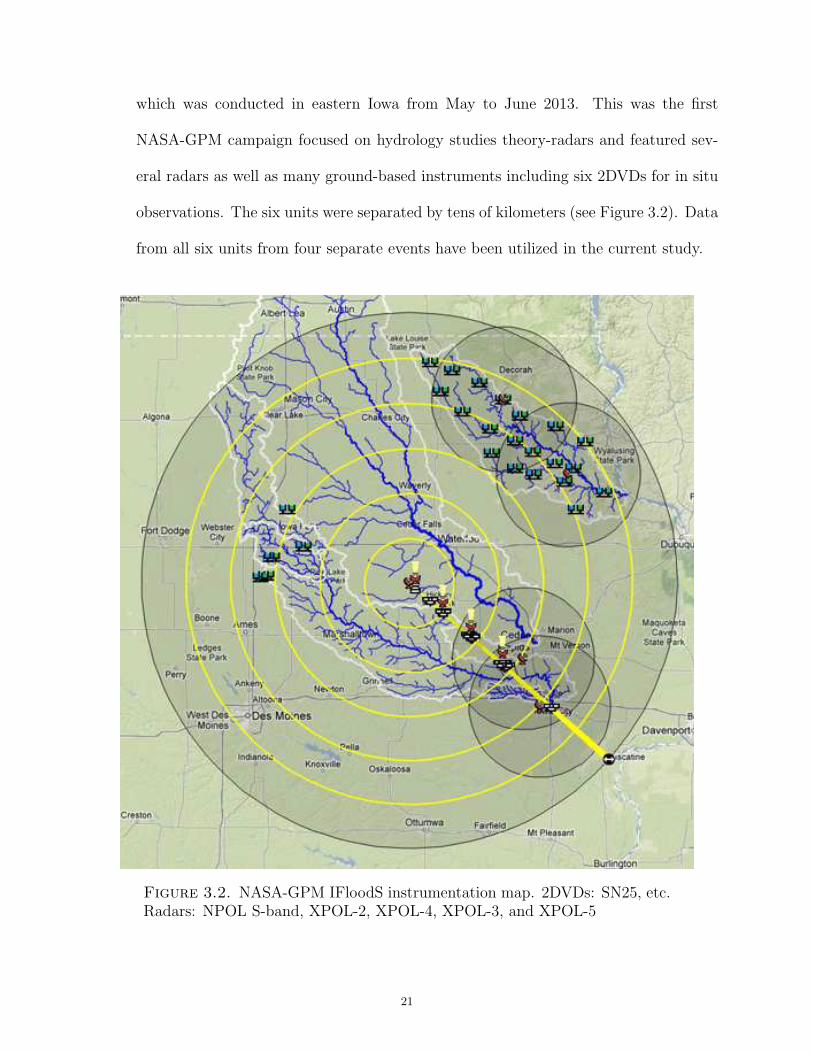
which was conducted in eastern Iowa from May to June 2013. This was the first

NASA-GPM campaign focused on hydrology studies theory-radars and featured sev-

eral radars as well as many ground-based instruments including six 2DVDs for in situ

observations. The six units were separated by tens of kilometers (see Figure 3.2). Data

from all six units from four separate events have been utilized in the current study.

Figure 3.2. NASA-GPM IFloodS instrumentation map. 2DVDs: SN25, etc.Radars: NPOL S-band, XPOL-2, XPOL-4, XPOL-3, and XPOL-5

21

III. Oklahoma (MC3E): The 2DVD data from Oklahoma were taken from the Mid-latitude

Continental Convective Clouds Experiment (MC3E; [15]) conducted in south-central

Oklahoma during the April to May 2011 period. This campaign also involved many

radars and ground instruments, including seven 2DVDs. Data from several events from

all seven units from this campaign were utilized in this study.

IV. Gan near Maldives (Gan): Whilst the above three represent mid-latitude, continental

climates, the fourth location considered in our study is an equatorial, location, situated

in the Indian ocean. Data used in this study were obtained from one 2DVD only

but over a 3.5 month period as part of the DYNAMO ((Dynamics of the Madden-

Julian Oscillation) field campaign (for example, [16]). Extensive analysis of the 3.5

month 2DVD dataset from this campaign has been recently completed [17]. One of

the interesting and important findings from this study is that the DSD characteristics

were very similar to those derived from another equatorial, oceanic location in the

Western Pacific, namely, Manus island. In both cases, the study found that DSDs

were characterized by small to medium drop diameters compared with continental

DSDs.

3.3. Comparison of the DSDs obtained from the Global data set

The computations presented herein, were obtained using 1-minute drop size distributions

(DSDs) from the four geographic locations, both independently and in a global sense. In

Figure 3.3, we illustrate the histograms of the mass-weighted mean diameters, Dm, and

the corresponding normalized intercept parameter, Nw, of the DSDs for each location as

compared to that of Gan and the Global dataset. From the Dm histograms in (a), (c), and

(d) note that the following points can be made, (i) the Gan DSDs are the most distinct with

22

a skew toward smaller drops and a tail showing fewer large drops, as expected for tropical

environments, (ii) the Global distribution is biased toward the DSDs of Huntsville, Alabama

(HSV) as this was a longer-term experiment where more diverse rain events were observed,

(iii) the distribution of MC3E followed the Global trend, as would be expected in continental

mid-latitudes in spring time, and (iv) the IFloodS Dm distribution is shifted to the right

due to the increased samples of larger drops observed during convective rain events during

the campaign. In Table 3.1, we summarize the mean and standard deviation of the Dm

distributions for the four locations, and see that the smallest mean and standard deviations

were measured in Gan, the largest mean Dm in IFloodS, with the largest spread (std. dev.=

0.504 mm) seen in MC3E.

Referring to the histograms (in b,d,f) and summarized statistics in the Table 3.1, one can

say almost all the normalized intercept parameters, Nw, are close to the Marshall-Palmer

(M-P) normalized intercept parameter for an exponential distribution of N0 = 3.9031 (i.e,

8, 000mm−1m−3), [18]. We should also note however, that the Nw for IFloodS is significantly

smaller than M-P, which is caused by the increased number of larger drops due to the more

convective nature of the dataset. It should be clear we are not discussing the actual shape of

the distributions (i.e., in terms of gamma parameters), but recognizing the DSD shapes can

be different, but still have intercept parameters near the exponential distribution of M-P. It

should also be noted that we are not separating the Dm’s based on rain types, as we note

the dominant convective events in IFloodS, while the other locations are composed of mixed

rain types primarily of stratiform and some convective events.

23

(a) Gan, HSV, Global DSDs (b) Gan, HSV, Global log10(Nw)

(c) Gan, IFloodS, Global DSDs (d) Gan, IFloodS, Global log10(Nw)

(e) Gan, MC3E, Global DSDs (f) Gan, MC3E, Global log10(Nw)

Figure 3.3. One-minute DSD comparisons between the following 2DVD lo-cations: (a,b) Gan, Huntsville (HSV), & Global datasets; (a,b) Gan, Iowa(IFloodS), & Global datasets; (e,f) Gan, Oklahoma (MC3E), & Globaldatasets. In the left column, mass-weighted mean diameter, Dm, of normalizedgamma DSDs, and in the right column are the normalized intercept paramters,as log10(Nw). Distributions are shown as % frequency of occurrence to easilycompare the different locations, with varying numbers of observations.

24

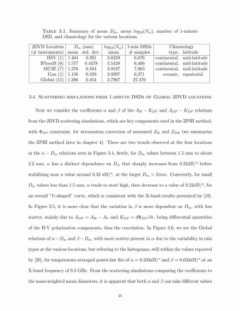
Table 3.1. Summary of mean Dm, mean log10(Nw), number of 1-minuteDSD, and climatology for the various locations.

2DVD Location Dm (mm) log10(Nw) 1-min DSDs Climatology(# instruments) mean std. dev. mean # samples type, latitude

HSV (1) 1.404 0.391 3.6259 6,876 continental, mid-latitudeIFloodS (6) 1.577 0.4478 3.5428 6,466 continental, mid-latitudeMC3E (7) 1.376 0.504 3.9187 7,863 continental, mid-latitudeGan (1) 1.156 0.359 3.9397 6,271 oceanic, equatorial

Global (15) 1.386 0.454 3.7907 27,476

3.4. Scattering simulations from 1-minute DSDs of Global 2DVD locations

Next we consider the coefficients α and β of the AH − KDP and ADP − KDP relations

from the 2DVD scattering simulations, which are key components used in the ZPHI method,

with ΦDP constraint, for attenuation correction of measured ZH and ZDR (we summarize

the ZPHI method later in chapter 4). There are two trends observed at the four locations

in the α −Dm relations seen in Figure 3.4, firstly, for Dm values between 1.5 mm to about

2.2 mm, α has a distinct dependence on Dm that sharply increases from 0.22dB/o before

stabilizing near a value around 0.32 dB/o, at the larger Dm > 2mm. Conversely, for small

Dm values less than 1.5 mm, α tends to start high, then decrease to a value of 0.22dB/o, for

an overall ”U-shaped” curve, which is consistent with the X-band results presented by [19].

In Figure 3.5, it is more clear that the variation in β is more dependent on Dm, with less

scatter, mainly due to ADP = AH − AV and KDP = dΦDP/dr, being differential quantities

of the H-V polarization components, thus the correlation. In Figure 3.6, we see the Global

relations of α−Dm and β−Dm, with more scatter present in α due to the variability in rain

types at the various locations, but referring to the histograms, still within the values reported

by [20], for temperature-averaged power-law fits of α = 0.233dB/o and β = 0.033dB/o at an

X-band frequency of 9.3 GHz. From the scattering simulations comparing the coefficients to

the mass-weighted mean diameters, it is apparent that both α and β can take different values

25

over the range of Dm’s, while in the Iterative ZPHI method, with ΦDP constraint, we find

a single optimal coefficient for the entire beam. This can lead to over/under estimation of

the attenuation (both AH and ADP ) along the beam, but can be improved by optimizing α

and β over shorter range intervals (i.e., dividing the full beam into segments), then applying

the estimation procedure over each interval, as proposed by [21]. The histograms for the

Global dataset are useful for providing a range of values for α and β, necessary for setting

the interval of optimal coefficient values in the iterative ZPHI method as proposed by [22],

for a large number of optimized beams.

In the attenuation correction procedure of the ZPHI method, we typically determine

the α & β coefficients from the slopes in the AH −KDP & ADP −KDP relations of 2DVD

scattering simulations, and typically do not compare their relation to the mass-weighted

mean diameters, Dm, as previously described. We should note that the slopes of α ≈ 0.30

from the mean fit in the AH −KDP relations, as illustrated in Figures 3.7 (and summarized

in Table 3.2), are not exactly equal to the mode Global α = 0.25 in the α −Dm histogram

(in Fig. 3.6). The variability in Dm is embedded in the AH data, so we optimize the α

coefficient in the ZPHI method to account for this variability and can tend to have higher

values. In Figures 3.8, we see more scatter in the ADP − KDP relations, even though this

ratio is derived from two differential quantities, which is apparent in the variability in β

values, summarized in Table 3.2 and in the absence of a distinct mode in the Global β vs.

Dm histogram (Fig. 3.6(b)). Figure 3.9, illustrates these AH −KDP & ADP −KDP relations

from scattering simulations using the Global dataset, which are in good agreement with the

relations of the independent locations.

26

(a) HSV (b) IFloodS

(c) Gan (d) MC3E

Figure 3.4. α coefficient vs. mass-weighted mean diameter, Dm, computedusing the one-minute DSDs from each 2DVD located in (a) Huntsville, AL(HSV), (b) Iowa (IFloodS), (c) Maldives (Gan), and (d) Oklahoma (MC3E)

3.5. Rain Rate algorithms derived from fits to scattering simulations

Various radar-derived rain rate algorithms, summarized in Table 3.3, can be derived by

applying a power law fit to the scattering simulations between the 2DVD-derived rain rates

27

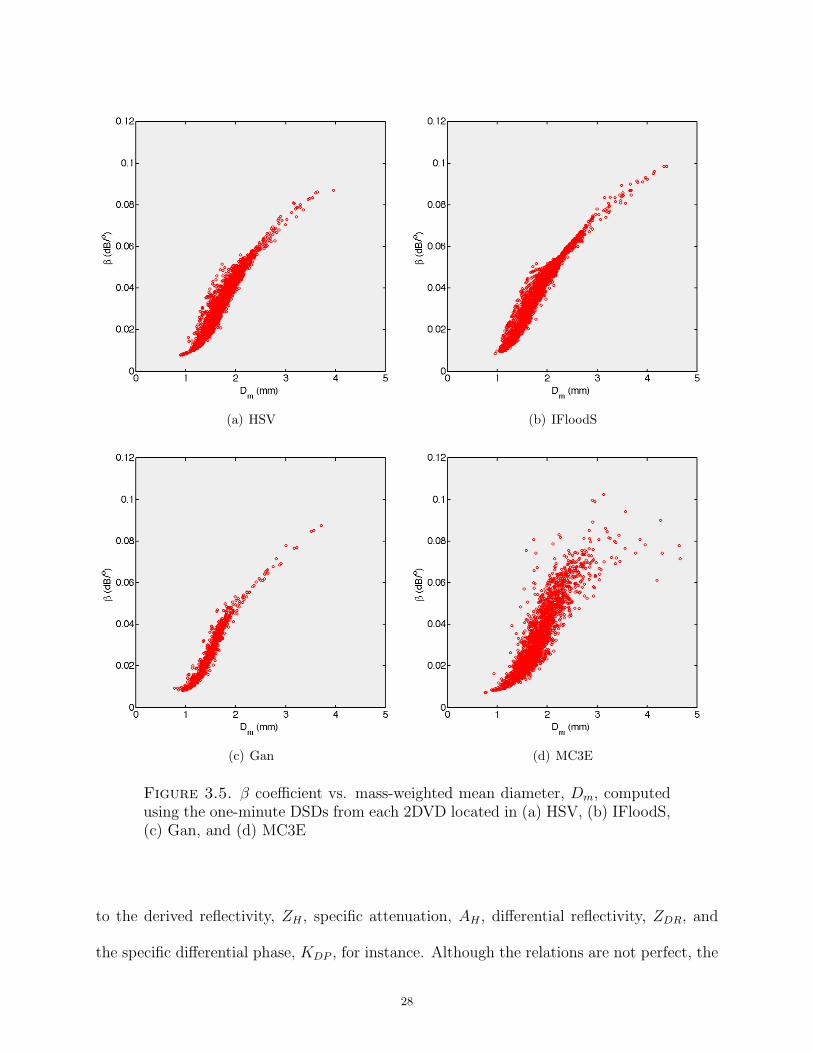
(a) HSV (b) IFloodS

(c) Gan (d) MC3E

Figure 3.5. β coefficient vs. mass-weighted mean diameter, Dm, computedusing the one-minute DSDs from each 2DVD located in (a) HSV, (b) IFloodS,(c) Gan, and (d) MC3E

to the derived reflectivity, ZH , specific attenuation, AH , differential reflectivity, ZDR, and

the specific differential phase, KDP , for instance. Although the relations are not perfect, the

28

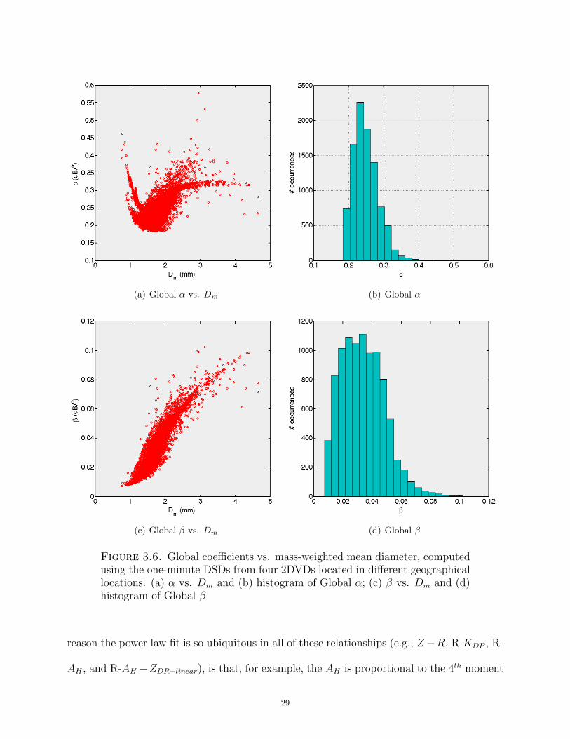
(a) Global α vs. Dm (b) Global α

(c) Global β vs. Dm (d) Global β

Figure 3.6. Global coefficients vs. mass-weighted mean diameter, computedusing the one-minute DSDs from four 2DVDs located in different geographicallocations. (a) α vs. Dm and (b) histogram of Global α; (c) β vs. Dm and (d)histogram of Global β

reason the power law fit is so ubiquitous in all of these relationships (e.g., Z−R, R-KDP , R-

AH , and R-AH −ZDR−linear), is that, for example, the AH is proportional to the 4th moment

29

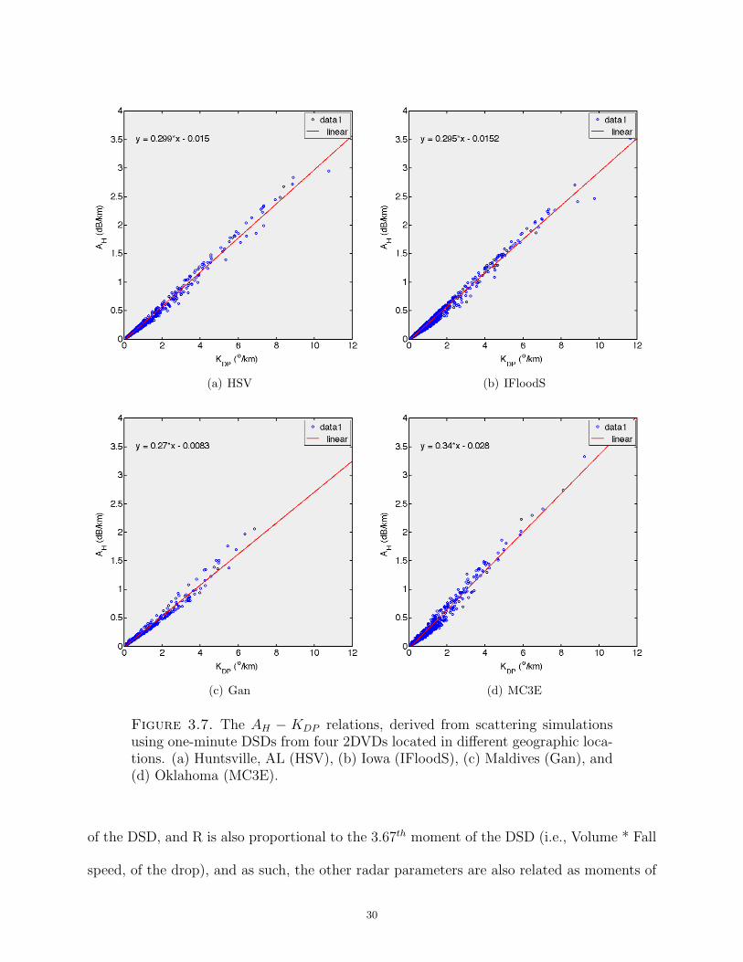
(a) HSV (b) IFloodS

(c) Gan (d) MC3E

Figure 3.7. The AH − KDP relations, derived from scattering simulationsusing one-minute DSDs from four 2DVDs located in different geographic loca-tions. (a) Huntsville, AL (HSV), (b) Iowa (IFloodS), (c) Maldives (Gan), and(d) Oklahoma (MC3E).

of the DSD, and R is also proportional to the 3.67th moment of the DSD (i.e., Volume * Fall

speed, of the drop), and as such, the other radar parameters are also related as moments of

30

(a) HSV (b) IFloodS

(c) Gan (d) MC3E

Figure 3.8. The ADP −KDP relations, derived from scattering simulationsusing one-minute DSDs from four 2DVDs located in different geographic loca-tions. (a) Huntsville, AL (HSV), (b) Iowa (IFloodS), (c) Maldives (Gan), and(d) Oklahoma (MC3E).

the drop size distribution. Scatter in the rain rate algorithms is primarily due to fluctuations

in the DSDs and Dm’s at each point.

31

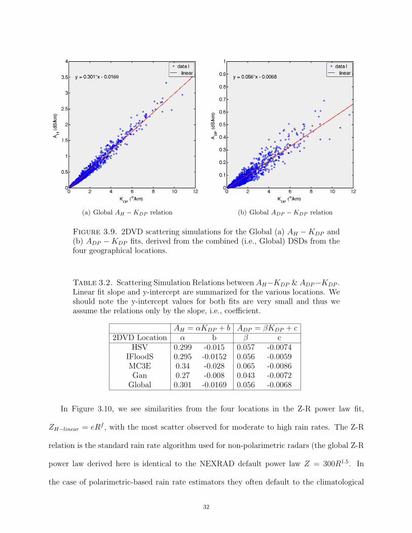
(a) Global AH −KDP relation (b) Global ADP −KDP relation

Figure 3.9. 2DVD scattering simulations for the Global (a) AH −KDP and(b) ADP −KDP fits, derived from the combined (i.e., Global) DSDs from thefour geographical locations.

Table 3.2. Scattering Simulation Relations betweenAH−KDP &ADP−KDP .Linear fit slope and y-intercept are summarized for the various locations. Weshould note the y-intercept values for both fits are very small and thus weassume the relations only by the slope, i.e., coefficient.

AH = αKDP + b ADP = βKDP + c2DVD Location α b β c

HSV 0.299 -0.015 0.057 -0.0074IFloodS 0.295 -0.0152 0.056 -0.0059MC3E 0.34 -0.028 0.065 -0.0086Gan 0.27 -0.008 0.043 -0.0072

Global 0.301 -0.0169 0.056 -0.0068

In Figure 3.10, we see similarities from the four locations in the Z-R power law fit,

ZH−linear = eRf , with the most scatter observed for moderate to high rain rates. The Z-R

relation is the standard rain rate algorithm used for non-polarimetric radars (the global Z-R

power law derived here is identical to the NEXRAD default power law Z = 300R1.5. In

the case of polarimetric-based rain rate estimators they often default to the climatological

32

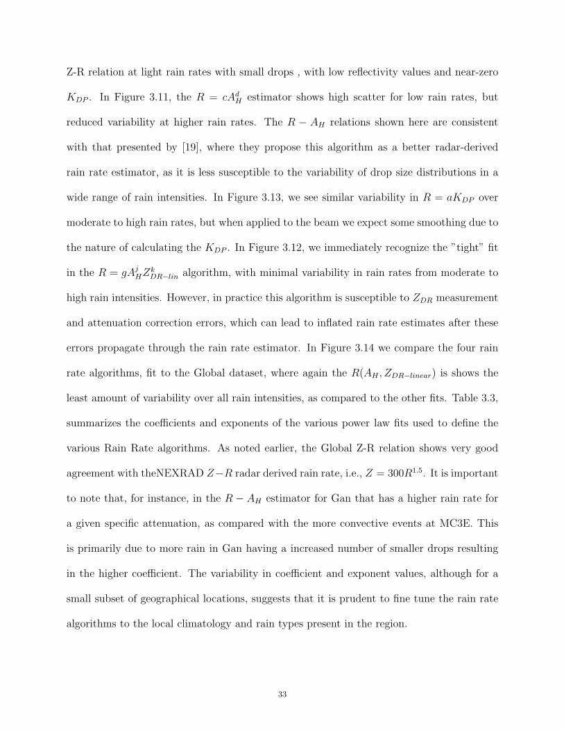
Z-R relation at light rain rates with small drops , with low reflectivity values and near-zero

KDP . In Figure 3.11, the R = cAdH estimator shows high scatter for low rain rates, but

reduced variability at higher rain rates. The R − AH relations shown here are consistent

with that presented by [19], where they propose this algorithm as a better radar-derived

rain rate estimator, as it is less susceptible to the variability of drop size distributions in a

wide range of rain intensities. In Figure 3.13, we see similar variability in R = aKDP over

moderate to high rain rates, but when applied to the beam we expect some smoothing due to

the nature of calculating the KDP . In Figure 3.12, we immediately recognize the ”tight” fit

in the R = gAjHZ

kDR−lin algorithm, with minimal variability in rain rates from moderate to

high rain intensities. However, in practice this algorithm is susceptible to ZDR measurement

and attenuation correction errors, which can lead to inflated rain rate estimates after these

errors propagate through the rain rate estimator. In Figure 3.14 we compare the four rain

rate algorithms, fit to the Global dataset, where again the R(AH , ZDR−linear) is shows the

least amount of variability over all rain intensities, as compared to the other fits. Table 3.3,

summarizes the coefficients and exponents of the various power law fits used to define the

various Rain Rate algorithms. As noted earlier, the Global Z-R relation shows very good

agreement with theNEXRAD Z−R radar derived rain rate, i.e., Z = 300R1.5. It is important

to note that, for instance, in the R − AH estimator for Gan that has a higher rain rate for

a given specific attenuation, as compared with the more convective events at MC3E. This

is primarily due to more rain in Gan having a increased number of smaller drops resulting

in the higher coefficient. The variability in coefficient and exponent values, although for a

small subset of geographical locations, suggests that it is prudent to fine tune the rain rate

algorithms to the local climatology and rain types present in the region.

33

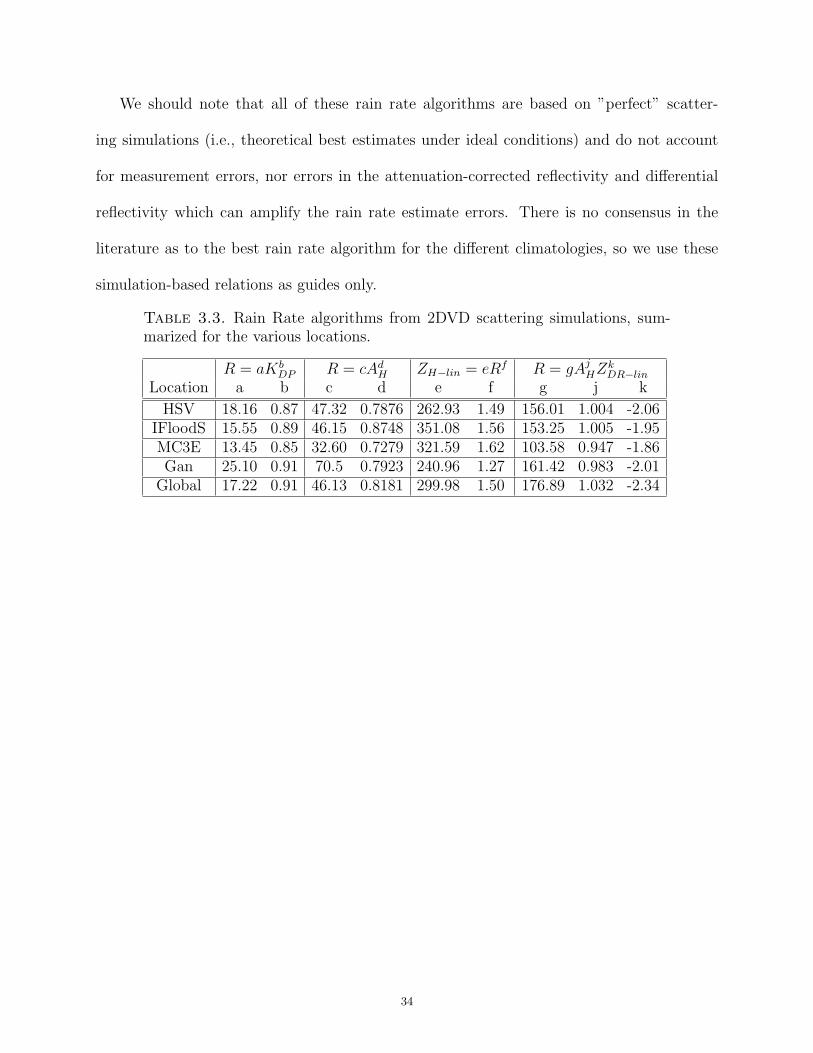
We should note that all of these rain rate algorithms are based on ”perfect” scatter-

ing simulations (i.e., theoretical best estimates under ideal conditions) and do not account

for measurement errors, nor errors in the attenuation-corrected reflectivity and differential

reflectivity which can amplify the rain rate estimate errors. There is no consensus in the

literature as to the best rain rate algorithm for the different climatologies, so we use these

simulation-based relations as guides only.

Table 3.3. Rain Rate algorithms from 2DVD scattering simulations, sum-marized for the various locations.

R = aKbDP R = cAd

H ZH−lin = eRf R = gAjHZ

kDR−lin

Location a b c d e f g j k

HSV 18.16 0.87 47.32 0.7876 262.93 1.49 156.01 1.004 -2.06IFloodS 15.55 0.89 46.15 0.8748 351.08 1.56 153.25 1.005 -1.95MC3E 13.45 0.85 32.60 0.7279 321.59 1.62 103.58 0.947 -1.86Gan 25.10 0.91 70.5 0.7923 240.96 1.27 161.42 0.983 -2.01

Global 17.22 0.91 46.13 0.8181 299.98 1.50 176.89 1.032 -2.34

34

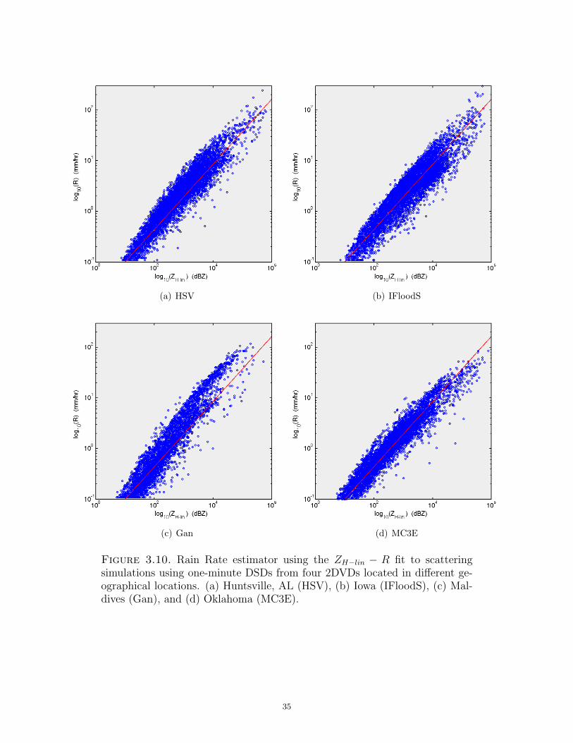
(a) HSV (b) IFloodS

(c) Gan (d) MC3E

Figure 3.10. Rain Rate estimator using the ZH−lin − R fit to scatteringsimulations using one-minute DSDs from four 2DVDs located in different ge-ographical locations. (a) Huntsville, AL (HSV), (b) Iowa (IFloodS), (c) Mal-dives (Gan), and (d) Oklahoma (MC3E).

35

(a) HSV (b) IFloodS

(c) Gan (d) MC3E

Figure 3.11. Rain Rate estimator R(AH) fit to scattering simulations usingone-minute DSDs from four 2DVDs located in different geographical locations.(a) Huntsville, AL (HSV), (b) Iowa (IFloodS), (c) Maldives (Gan), and (d)Oklahoma (MC3E).

36

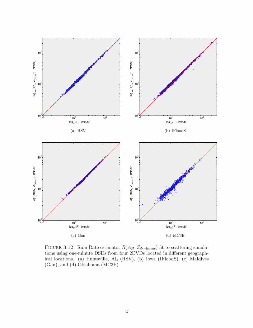
(a) HSV (b) IFloodS

(c) Gan (d) MC3E

Figure 3.12. Rain Rate estimator R(AH , Zdr−linear) fit to scattering simula-tions using one-minute DSDs from four 2DVDs located in different geograph-ical locations. (a) Huntsville, AL (HSV), (b) Iowa (IFloodS), (c) Maldives(Gan), and (d) Oklahoma (MC3E).

37

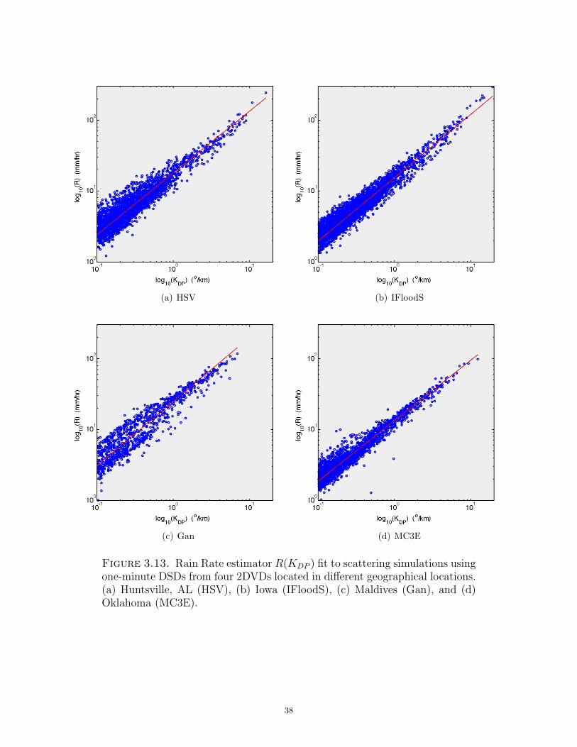
(a) HSV (b) IFloodS

(c) Gan (d) MC3E

Figure 3.13. Rain Rate estimator R(KDP ) fit to scattering simulations usingone-minute DSDs from four 2DVDs located in different geographical locations.(a) Huntsville, AL (HSV), (b) Iowa (IFloodS), (c) Maldives (Gan), and (d)Oklahoma (MC3E).

38

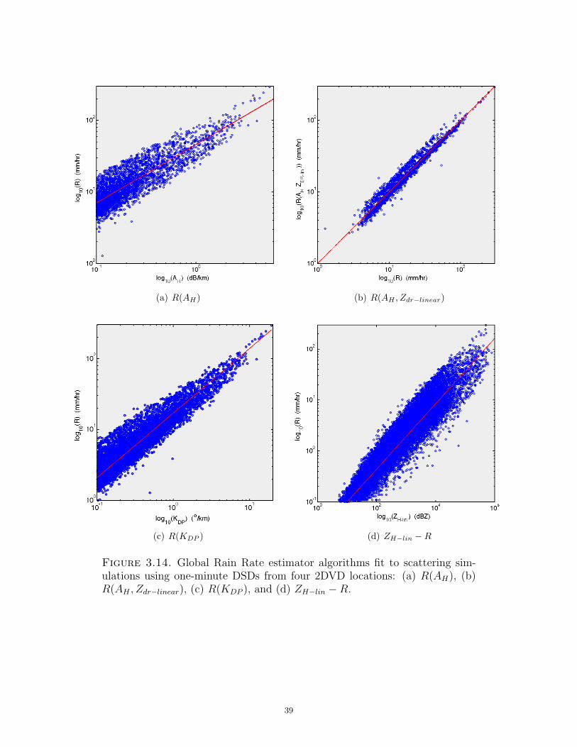
(a) R(AH) (b) R(AH , Zdr−linear)

(c) R(KDP ) (d) ZH−lin −R

Figure 3.14. Global Rain Rate estimator algorithms fit to scattering sim-ulations using one-minute DSDs from four 2DVD locations: (a) R(AH), (b)R(AH , Zdr−linear), (c) R(KDP ), and (d) ZH−lin −R.

39

CHAPTER 4

Attenuation Correction using the iterative ZPHI

Method and an improved differential backscatter

phase estimator

In this Chapter, we will introduce the attenuation-correction procedure applied to the

Iowa XPOL radar data collected during the NASA GPM IFloodS field campaign. We share

the summarized description of the ZPHI method, with ΦDP constraint for attenuation cor-

rection at X-band, as presented in our article in the Journal of Hydrometeorology titled,

”Deployment and Performance Analyses of High Resolution Iowa XPOL Radar System dur-

ing the NASA IFloodS Campaign” [23]. In addition, we present an iterative FIR range filter

designed for X-band radars with high range resolution (∆r=30m), based on a method pro-

posed by Hubbert and Bringi (1995) for systems operating at ∆r=150m, providing improved

estimation of differential backscatter phase, δ, at these shorter range intervals. We introduce

the attenuation correction procedures and filter design here, and in chapter 5 will present

results from data observed during the IFloodS field campaign.

4.1. Summary of Attenuation Correction Procedure

At frequencies above S-band (10 cm), radar operating wavelengths decrease and correc-

tion of the measured reflectivity, ZH , and differential reflectivity, ZDR, due to rain attenuation

along the propagation path becomes essential, particularly at X-band (3.2 cm) in convective

storms. The method used herein for correcting the measured ZH is an iterative version of

the ZPHI method which uses a ΦDP constraint [24, 25], initially developed at C-band then

later extended to X-band by [26, 22]. In brief, the coefficient α is the linear relation between

40

specific attenuation at horizontal polarization (AH) and specific differential phase (KDP ),

approximately AH = αKDP . This optimal coefficient is determined by minimizing a cost

function (we refer to [2] for details), whereas the standard ZPHI method assumes an a priori

fixed value for α [24]. In the modified ZPHI method, the optimal α obtained from this iter-

ative process, overcomes its dependence on temperature and any potential deviations of the

raindrop oblateness model from equilibrium theory [27]. There is additional compensation

for drop size distributions, DSDs, with above average values of D0 (median volume diame-

ters > 2.5 mm or so). it is important to note that like all attenuation-correction algorithms

based on ΦDP , the correction is an approximation since the true DSD along the propagation

path is not known. In essence, we obtain the optimal α and fix it for the entire beam, on

a ray-by-ray basis, using the algorithm described in [22] with modifications for the higher

range resolution (∆r=30 m) of the XPOL radar systems. Improvements in determining the

optimal α are possible if the full beam is divided into smaller range intervals, then applying

the estimation procedure to yield an optimal α coefficient for each sub-interval [21]. There

are other alternatives of the attenuation-correction method at X-band, as elucidated, for

example, by [28], [29], and [30].

The correction of the measured differential reflectivity, ZDR, for specific differential at-

tenuation (ADP ) is based on a method proposed by Smyth and Illingworth [31] for C-band,

which is described in [2] as a ”combined ΦDP −ZDR constraint.” This method was later ex-

tended to X-band by Park et al. (2005 II) which is used herein with modifications tuned for

the Iowa XPOL radars. In brief, the previously determined specific horizontal attenuation

AH using the ΦDP constraint is scaled by a factor γ, and the measured ZDR is corrected for

the differential attenuation (ADP = γAH), such that a desired value is reached at the end

of the beam. The desired value is the intrinsic or ’true’ ZDR value at the end of the beam,

41

which is estimated from the corrected ZH via a mean ZH-ZDR relation based on scattering

simulations that use measured drop size distributions (DSDs) from several locations in east-

ern Iowa, representing a wide variety of rain types. This sets a constraint for ZDR at the

end of the beam (generally the ZDR ≈ 0 dB is due to light rain at the end of the beam or

due to ice particles above the 0o C level). The end of the beam is defined as the last range

gate where ”meteo” echoes are detected. Like before, the differential attenuation-correction

is approximate since the true DSD along the beam is unknown. Kim et al. (2010) proposed

a method to correct for ZDR by using the ZPHI method to independently estimate AH and

AV (i.e., via the optimal coefficients αH and αV ; note that ADP = AH −AV ) without using

an explicit ZDR constraint at the end of the beam.

4.2. Data processing steps for the attenuation-correction procedure

The processing steps used to correct the measured ZH and ZDR for XPOL data closely

follow that proposed by [32, 33], and hence, we only summarize them here.

I. On a ray-by-ray basis, we generate a data mask along each range profile to separate

precipitation (’meteo’=1) from non-precipitation (’non-meteo’=0) echoes using the

standard deviation of ΦDP over a 10-gate moving window. The classification is based

on using a threshold of 5◦ and an SNR > 0 dB, and may sometimes be referred to as

the ’good data mask.’

II. We correct the measured ZH and ZDR values for attenuation, as previously described.

III. To derive the specific differential phase, KDP , we first use the iterative range filter

methodology applied to each range profile of ΨDP . The finite impulse response (FIR)

range filter is, in essence, a weighted moving average filter where the weights are deter-

mined by the desired magnitude response of the filter transfer function (or spectrum).

42

Here, the FIR filter coefficients are based on a 75 m range gate spacing (an example of

the filter transfer function for 150 m gate spacing can be found in [34]). It is important

to note that for this study of the IFloodS data from XPOL-4, the range gate spacing

was 30 m. The iterative nature of the algorithm described in Hubbert and Bringi (1995)

is designed to remove local perturbations in the ΨDP data (e.g., due to backscatter

differential phase) while still preserving the monotonic increase in propagation phase

(ΦDP ) with range, along the beam. The copolar differential phase, ΨDP , consists of

two phase components, that include the differential propagation phase, ΦDP , and the

differential backscatter phase, δ. We will consider the estimation of these perturba-

tions later in this chapter. A ”telescoping’” method is used to compute the KDP from

the iteratively filtered ΦDP profile, that is, a variable number of range gates is used,

depending on the ZH value, to determine the slope of a linear least squares fit. Selec-

tion of the telescoping gate number is as follows: 10 gates if ZH > 35 dBZ; 20 gates

if 25 < ZH < 35 dBZ; and 30 gates if ZH < 25 dBZ. The telescoping method can

be considered ad hoc, but has good agreement with the light (9 gates) and heavy (25

gates) filtering for computing KDP discussed by [35].

Since the data processing progresses one beam (or range profile) at a time, we illustrate

in Figure 4.1 range profiles of (a) the measured and attenuation-corrected ZH , and the same

for (b) ZDR. The path integrated attenuation (PIA= corrected - measured, across the rain

cell) from 0-20 km is around 14 dB, while the path integrated differential attenuation is

around 2.7 dB. This sample beam is at an azimuth angle of 310◦ and elevation angle of

10.7◦, as indicated by the dashed lines in Figure 5.4. Panel (c) shows the monotonically

increasing ΦDP with range, the overall difference across the rain cell is around ∆ΦDP = 40◦.

The filtered propagation phase, ΦDP−filt, is also shown from which KDP is calculated. The

43

coefficient α, of the AH − KDP relation, can be estimated as α ≈PIA/∆ΦDP−filt over the

rain cell range interval. For this range profile α=14/40=0.35 dB/deg, whereas the coefficient

β (in ADP −KDP ) is 2.7/40 = 0.067 dB/deg. Panel (d) shows the KDP profile seeing a peak

of 5.6 ◦/km at a range of 12 km; the corresponding corrected ZH and ZDR are 52.8 dBZ and

2.2 dB, respectively. Also shown in this panel is the data mask indicating the occurrence of

precipitation echoes (1 ≡’meteo’, 0 ≡’non-meteo’ echoes).

The rain rate from KDP can be derived from R = 14.2K0.85DP , which gives 60 mm/hr

whereas the ZH = 320R1.55, with ZH=52.8 dBZ, also gives close to 60 mm/hr. The co-

efficients and exponents of the R(KDP ) and R(ZH) power laws are derived from 2D-video

disdrometer measured DSDs from four days during IFloodS, and scattering simulations us-

ing the T-matrix method, assuming the 80 m fall bridge shapes from [36] and Gaussian

distribution of canting angles with [µ = 0◦; σ = 7.5◦] from [37]. The agreement between

the calculated rain rates, R(KDP ) and R(ZH), for the 12 km range gate is perhaps coin-

cidental but it affirms that the ZH attenuation-correction is reasonable (if the measured

ZH = 42 dBZ had been used, the corresponding R would have been severely underestimated

at 12 mm/hr). This result attests to the established importance of attenuation correction

at X-band particularly if Z-R relations are subsequently used to quantify rainfall amounts.

4.3. Iterative FIR range filter design for X-band radars operating at high

range resolutions of ∆r=30m

The copolar differential phase, ΨDP , measurement is of utmost importance and uniquely

inherent to dual polarization radars. It has the advantage over reflectivity and differential

reflectivity in that it is not adversely affected by attenuation along the propagation path

44

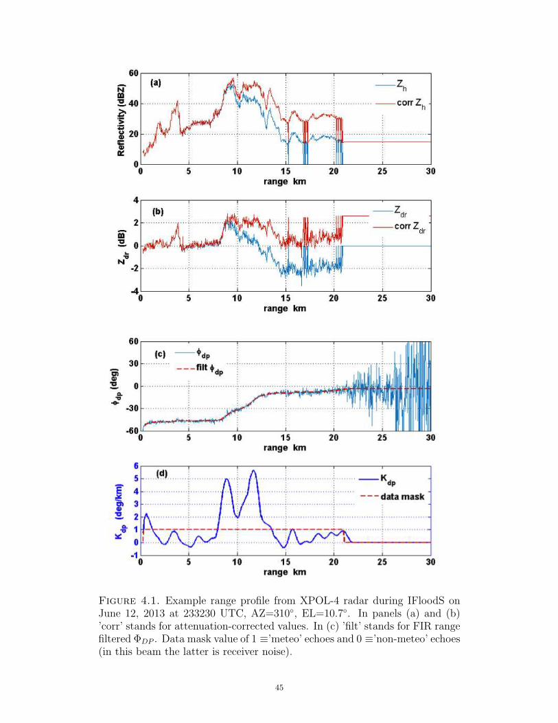
Figure 4.1. Example range profile from XPOL-4 radar during IFloodS onJune 12, 2013 at 233230 UTC, AZ=310◦, EL=10.7◦. In panels (a) and (b)’corr’ stands for attenuation-corrected values. In (c) ’filt’ stands for FIR rangefiltered ΦDP . Data mask value of 1 ≡’meteo’ echoes and 0 ≡’non-meteo’ echoes(in this beam the latter is receiver noise).

45

through precipitation, nor to radar calibration issues. It is composed of two phase compo-

nents, one being the range cumulative differential propagation phase, ΦDP , and the other is

due to scattering effects at each range resolution volume, known as differential backscatter

phase, δ. In a purely rain event, ΨDP is dominated by ΦDP , and we can easily rely on the

computed slope of the copolar differential phase, i.e., specific differential phase KDP , to es-

timate the rain rate and rainwater content. On the contrary, in the presence of melting hail

or Mie scattering effects, δ becomes increasingly more significant in the copolar differential

phase (ΨDP = ΦDP + δ) which leads to local perturbations or ”bumps” in the normally

monotonic increasing ΨDP along the range. These δ bumps bias the estimated KDP and

lead to subsequent errors in estimations of rain rate and rainwater content. Unlike radars

operating at S-band (10 cm), the effects due to Mie scattering are very relevant to hydrology

studies using dual polarization Doppler weather radars operating at shorter wavelengths, like

those at X-band (3.2 cm) and C-band (5 cm), for instance. In order to ensure accurate rain

rate estimates based on KDP at X-band, it is imperative that the δ is properly separated

from the copolar differential phase measurement before computing specific differential phase.

For our filter design, we refer to the iterative range filtering technique developed by [34]

(henceforth, H&B-95) for the analysis of ΨDP and dual-wavelength radar measurements,

which has successfully proven to mitigate the local perturbations due to differential backscat-

ter phase, in the monotonically increasing differential phase of radars operating with range

resolutions of ∆r= 75 - 150 m. Most polarimetric weather radars operating in the 5 cm to

10 cm wavelength regime (C-band & S-band), typically use these coarse range resolution

intervals as a trade-off to increase the maximum achievable unambiguous scanning range,

as limited by the radar PRF and the sampling frequency of the digital signal processor.

Over the past decade, the use of X-band dual polarization radars has gained acceptance as a

46

complementary technology to the legacy S- & C-band radars used by the meteorological and

hydrology communities. For instance, X-band polarimetric radars have been used in high

spatio-temporal hydrology studies [23], warning systems for flooding and shallow landslide

forecasting in urban areas [38], and configured in cooperative networks for urban and rural

settings [39, 40], to combat the effects of signal extinction experienced by individual radars,

at shorter wavelengths. These X-band radars are being operated with much higher range

resolutions, for instance at a ∆r = 30m or less, like the University of Iowa XPOL radars.

We begin by evaluating the effectiveness of applying various iterative FIR range filters

to a raw ΨDP range profile as observed by the XPOL-4 radar system during the IFloodS

field campaign. Figure 4.2 compares the filtering performance of three iterated lowpass FIR

range filters used to suppress the δ, all being lowpass FIR filters: (magenta) 40th order 75 m

Butterworth of H&B-95, (black) 40th order 30 m Kaiser, and (green) 100th order 30 m Kaiser

filters. We can clearly see similarities in δ-suppression between the 40th order FIR range

filters (75 m & 30 m), although each was designed for a different spatial sampling period,

the number of coefficients are the same. The coefficients of the H&B-95 FIR Butterworth

filter were optimized for ∆r of 75 to 150 meter intervals, which when applied to the much

higher range resolution XPOL radar data, cannot effectively suppress the ”bumps” in the

monotonically increasing ΨDP , due to melting hail or Mie scattering effects. The superior

δ-suppression rendered by the 100th order 30 m Kaiser lowpass FIR range filter is obvious

in this range profile segment, and we will further discuss its design and a two-stage filtering

process to further optimize it over the entire beam.

The Kaiser (or Kaiser-Bessel) finite impulse response (FIR) filter was selected from among

several window functions that minimize the passband ripple by decreasing the sidelobes of

the window transfer function. It is well known in the literature that a rectangular window

47

Figure 4.2. FIR30m-100 filter shows improvement in the ability to mitigateMie backscattering between 20-24 km from the ΦDP range profile through aconvective storm. Radar data from a low elevation (EL = 3o) XPOL-4 PPIscan, at AZ = 287o, during IFloodS on 20130612-2327 UTC.

transfer function has very large sidelobes, at about -13 dB down from the main lobe, but

on the contrary the Kaiser family of windows are optimized such that most of the energy is

in its main lobe for a given side-lobe amplitude. The Kaiser window can be defined by (see

[41, 42] for details),

(4.1) w(n) =

I0

[

βK

√

1− (n−p

p)2]

I0(βK), 0 ≤ n ≤ N

where p=(N-1)/2, and I0(*) is a zeroth-order modified Bessel function of the first kind, which

can be generated using the power series expansion,

(4.2) I0(x) = 1 +∞∑

k=1

(x/2)k

k!

48

The βK parameter determines the shape of the window and controls the main lobe width

and side-lobe amplitude δs. The relationship between the βK parameter and stopband ripple

of a lowpass filter, αs = −20log(δs−linear) can be determined as,

(4.3) βK =

0.1102(αs − 8.7) αs > 50

0.5842(αs − 21)0.4 + 0.07886(αs − 21) 21 ≤ αs ≤ 50

0.0 αs < 21

and to meet our design criteria, we used a βK = 3.2, which yielded a minimum sidelobe

attenuation of δs = 25 dB, and a stopband ripple αs = 52 dB. In order to ”fine-tune” the

filter, we used Matlab’s Filter Design & Analysis Tool (FDATool), of the Signal Processing

Toolbox, which saved time and made it simple to evaluate various other windows. We use

this criteria for the design of both the 100th and 40th order FIR filters for the high spatial

sampling of the XPOL radars (i.e., ∆r= 0.030 km).

For the original attenuation-correction procedure, we applied the available 40th order

”FIR75M” filter to the XPOL-4 data with ∆r=0.030 km, as mentioned in a previous section,

where essentially we are applying a weighted moving average about each range sample, over a

±600 meter window. Because we wanted better differential backscatter phase, δ, estimation

we began to investigate the response of an equivalent Kaiser FIR filter. In Figure 4.3 we

illustrate the magnitude response of the 40th order 30 m Kaiser lowpass FIR range filter,

initially designed as the replacement for the Butterworth filter of H&B-95 (see [34], for an

example 20th order filter, based on a 150 m spatial sampling period). The Kaiser FIR filter

maintains the sharp attenuation (minimum of 25 dB) of spatial variations in the stopband,

in this case over an interval of 0.4215 km or less based on the 0.030 km spatial sample period.

Referring again to Figure 4.2, we see that 40 coefficients provide insufficient mitigation of the

49

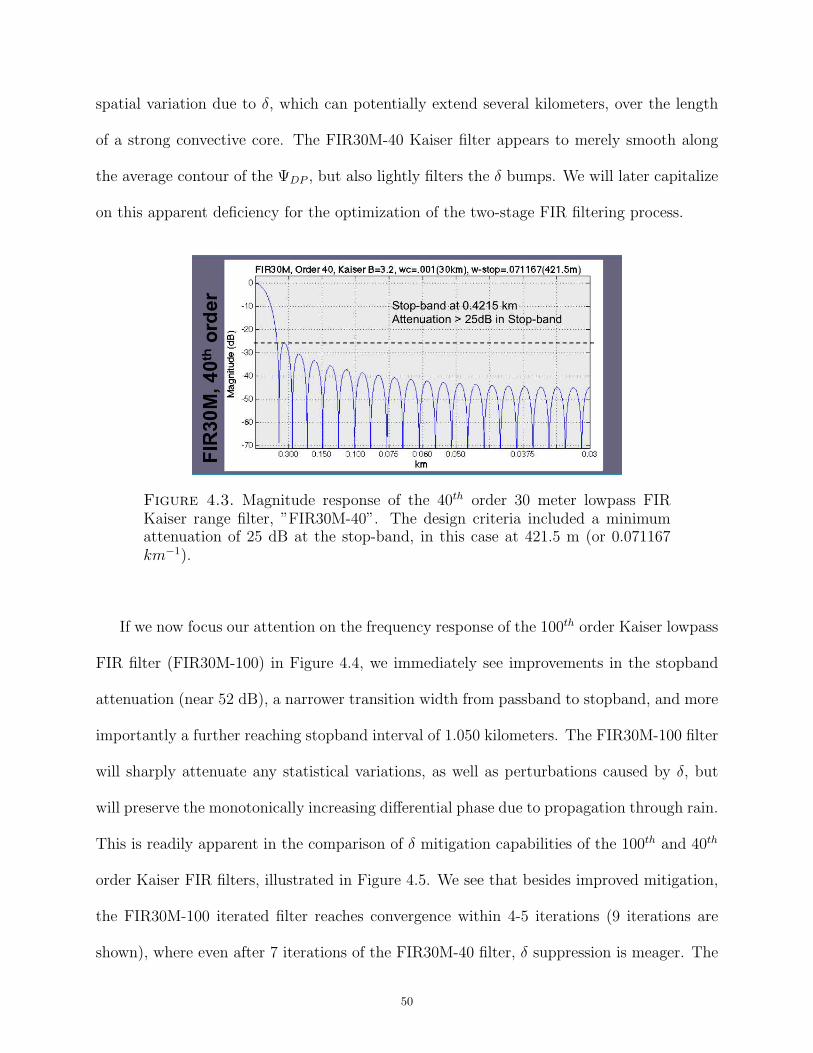
spatial variation due to δ, which can potentially extend several kilometers, over the length

of a strong convective core. The FIR30M-40 Kaiser filter appears to merely smooth along

the average contour of the ΨDP , but also lightly filters the δ bumps. We will later capitalize

on this apparent deficiency for the optimization of the two-stage FIR filtering process.

Figure 4.3. Magnitude response of the 40th order 30 meter lowpass FIRKaiser range filter, ”FIR30M-40”. The design criteria included a minimumattenuation of 25 dB at the stop-band, in this case at 421.5 m (or 0.071167km−1).

If we now focus our attention on the frequency response of the 100th order Kaiser lowpass

FIR filter (FIR30M-100) in Figure 4.4, we immediately see improvements in the stopband

attenuation (near 52 dB), a narrower transition width from passband to stopband, and more

importantly a further reaching stopband interval of 1.050 kilometers. The FIR30M-100 filter

will sharply attenuate any statistical variations, as well as perturbations caused by δ, but

will preserve the monotonically increasing differential phase due to propagation through rain.

This is readily apparent in the comparison of δ mitigation capabilities of the 100th and 40th

order Kaiser FIR filters, illustrated in Figure 4.5. We see that besides improved mitigation,

the FIR30M-100 iterated filter reaches convergence within 4-5 iterations (9 iterations are

shown), where even after 7 iterations of the FIR30M-40 filter, δ suppression is meager. The

50

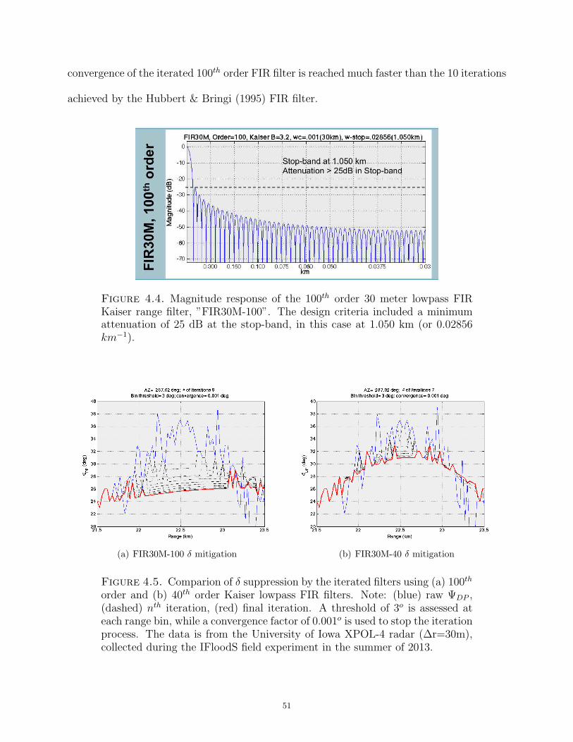
convergence of the iterated 100th order FIR filter is reached much faster than the 10 iterations

achieved by the Hubbert & Bringi (1995) FIR filter.

Figure 4.4. Magnitude response of the 100th order 30 meter lowpass FIRKaiser range filter, ”FIR30M-100”. The design criteria included a minimumattenuation of 25 dB at the stop-band, in this case at 1.050 km (or 0.02856km−1).

(a) FIR30M-100 δ mitigation (b) FIR30M-40 δ mitigation

Figure 4.5. Comparion of δ suppression by the iterated filters using (a) 100th

order and (b) 40th order Kaiser lowpass FIR filters. Note: (blue) raw ΨDP ,(dashed) nth iteration, (red) final iteration. A threshold of 3o is assessed ateach range bin, while a convergence factor of 0.001o is used to stop the iterationprocess. The data is from the University of Iowa XPOL-4 radar (∆r=30m),collected during the IFloodS field experiment in the summer of 2013.

51

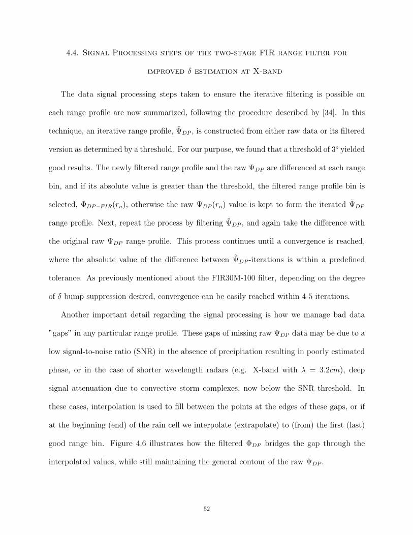
4.4. Signal Processing steps of the two-stage FIR range filter for

improved δ estimation at X-band

The data signal processing steps taken to ensure the iterative filtering is possible on

each range profile are now summarized, following the procedure described by [34]. In this

technique, an iterative range profile, ΨDP , is constructed from either raw data or its filtered

version as determined by a threshold. For our purpose, we found that a threshold of 3o yielded

good results. The newly filtered range profile and the raw ΨDP are differenced at each range

bin, and if its absolute value is greater than the threshold, the filtered range profile bin is

selected, ΦDP−FIR(rn), otherwise the raw ΨDP (rn) value is kept to form the iterated ΨDP

range profile. Next, repeat the process by filtering ΨDP , and again take the difference with

the original raw ΨDP range profile. This process continues until a convergence is reached,

where the absolute value of the difference between ΨDP -iterations is within a predefined

tolerance. As previously mentioned about the FIR30M-100 filter, depending on the degree

of δ bump suppression desired, convergence can be easily reached within 4-5 iterations.

Another important detail regarding the signal processing is how we manage bad data

”gaps” in any particular range profile. These gaps of missing raw ΨDP data may be due to a

low signal-to-noise ratio (SNR) in the absence of precipitation resulting in poorly estimated

phase, or in the case of shorter wavelength radars (e.g. X-band with λ = 3.2cm), deep

signal attenuation due to convective storm complexes, now below the SNR threshold. In

these cases, interpolation is used to fill between the points at the edges of these gaps, or if

at the beginning (end) of the rain cell we interpolate (extrapolate) to (from) the first (last)

good range bin. Figure 4.6 illustrates how the filtered ΦDP bridges the gap through the

interpolated values, while still maintaining the general contour of the raw ΨDP .

52

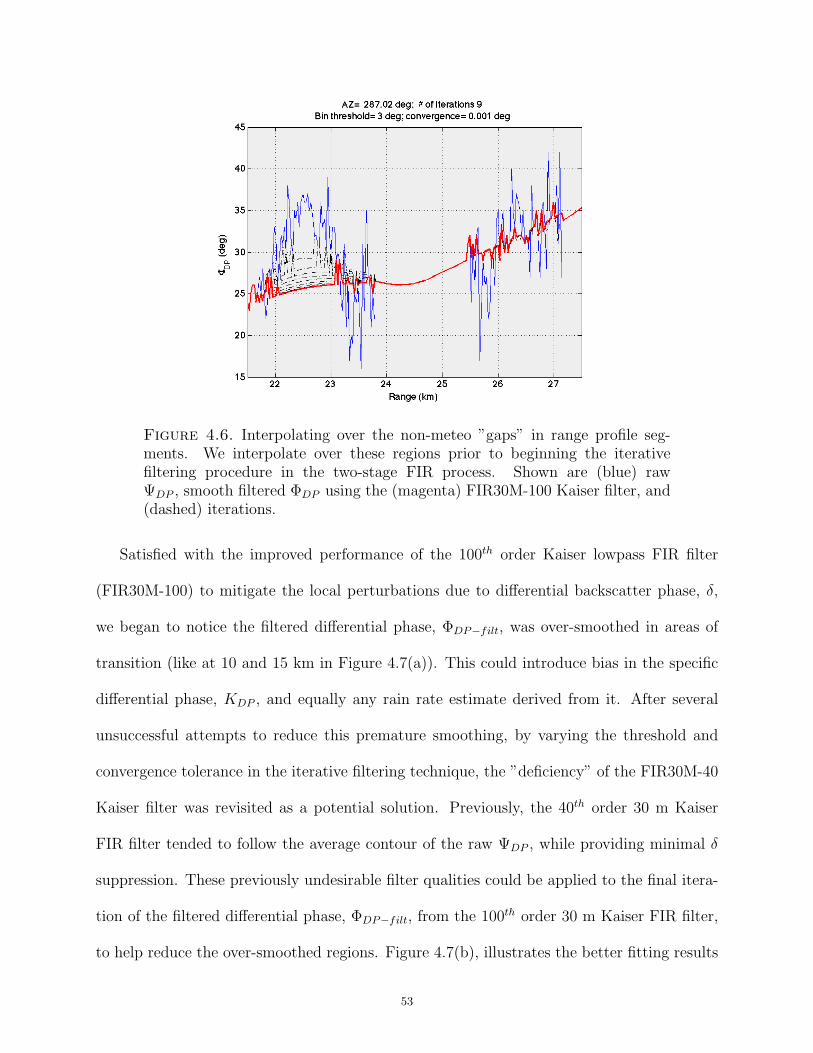
Figure 4.6. Interpolating over the non-meteo ”gaps” in range profile seg-ments. We interpolate over these regions prior to beginning the iterativefiltering procedure in the two-stage FIR process. Shown are (blue) rawΨDP , smooth filtered ΦDP using the (magenta) FIR30M-100 Kaiser filter, and(dashed) iterations.

Satisfied with the improved performance of the 100th order Kaiser lowpass FIR filter

(FIR30M-100) to mitigate the local perturbations due to differential backscatter phase, δ,

we began to notice the filtered differential phase, ΦDP−filt, was over-smoothed in areas of

transition (like at 10 and 15 km in Figure 4.7(a)). This could introduce bias in the specific

differential phase, KDP , and equally any rain rate estimate derived from it. After several

unsuccessful attempts to reduce this premature smoothing, by varying the threshold and

convergence tolerance in the iterative filtering technique, the ”deficiency” of the FIR30M-40

Kaiser filter was revisited as a potential solution. Previously, the 40th order 30 m Kaiser

FIR filter tended to follow the average contour of the raw ΨDP , while providing minimal δ

suppression. These previously undesirable filter qualities could be applied to the final itera-

tion of the filtered differential phase, ΦDP−filt, from the 100th order 30 m Kaiser FIR filter,

to help reduce the over-smoothed regions. Figure 4.7(b), illustrates the better fitting results

53

by implementing this two-stage FIR range filtering technique which ultimately enhances dif-

ferential backscatter phase estimation, where δ = raw ΨDP − ΦDP−filt. Better estimates of

differential backscatter phase at X-band can lead to improvements in estimating the KDP ,

and in determining rain rates and rainwater content when using KDP -based algorithms. In

Chapter 5, further exploration is conducted into the effects of applying the two-stage FIR

filtering technique to better estimate the δ signal.

(a) FIR30M-100 final filtered iteration (b) Two-stage smooth filtered ΦDP−filt

Figure 4.7. Range profile through a convective storm complex. In both,raw ΨDP is (blue); (a) is the Final iteratively filtered ΦDP−iter100 using theFIR30M-100 Kaiser filter (red), and in (b) the resulting two-stage smooth fil-tered ΦDP−2FIR (magenta) after a single application of the FIR30M-40 KaiserFIR to the Final iteratively filtered ΦDP−iter100 of (a). Radar data from IowaXPOL-4 PPI at AZ=287 & EL=3, observed during IFloodS field campaign on12 June 2013 at 23:27 UTC.

Now, considering the estimated differential backscatter phase ”δ” obtained by applying

the two-stage 100th order 30 m FIR lowpass range filter, improved detection of the local

perturbation due to Mie scattering can clearly be seen. In Figure 4.8(b), the detection of

backscatter phase is visible between 22-24 km down range from the radar, and also a small δ

54

around 11-13 km. Comparing it to the 40th order 75 m FIR lowpass range filter of Hubbert

& Bringi (1995), the ”δ” estimator using the new 2-stage FIR filtering of the ΨDP shows

an appreciable improvement. This is due to the enhanced ”δ” mitigation in the filtering

of the raw copolar differential phase, evident in the comparison of the range profiles in

Figure 4.8(a). Illustrated in panel (c) are overlaid scatter plots showing the relation between

δ and ZDR−cor for the two filtering methods. Again, the improved estimation of the 2-stage

FIR filtering is evident by the higher concentration of δ’s values greater than 4o, indicating

better detection of Mie scattering. The histograms of panel (d) confirm the better detection

by the higher number of occurrences for the proposed filter. The δ−ZDR−cor relation of the

2-stage FIR filter shows good agreement with the results obtained by [43], which are similar

to the theoretical relationships for rain.

The enhanced differential backscatter phase estimation, using the proposed two-stage

FIR lowpass filtering technique, has implications at X-band where Mie scattering can be

experienced in moderate to severe rain. Estimation and detection of the backscatter phase

can be used to improve specific differential phase, KDP , and rain rate estimation, as well as

aid in microphysical retrievals, as suggested for low elevation scans by [43].

55

(a) (b)

(c) (d)

Figure 4.8. Estimated differential backscatter phase ”δ” comparison be-tween the proposed 2-stage FIR lowpass filter and the 75m FIR lowpass filterof Hubbert & Bringi (1995), H-B 95, when applied to the higher 30 m rangeresolution data of the XPOL-4. (a) Raw and filtered ΦDP using both 2-stageFIR & FIR75m filters; (b) δ estimation, r=16-24 km; (c) δ vs. ZDR−cor scatterplot for the AZ = 287o ray profile; (d) Histogram of δ > 4o & ZDR−cor > 1 dBfor the ray profile. Radar data from Iowa XPOL-4 PPI at AZ=287 & EL=3,observed on 20130612-2327 UTC during the IFloodS field campaign.

56

CHAPTER 5

Results and comparative analyses of

attenuation-corrected XPOL radar data collected

during the NASA GPM IFloodS field campaign

During the spring of 2013, the Iowa Flood Studies (IFloodS) field campaign was con-

ducted in central and northeastern Iowa as an integral component of the Ground Validation

(GV) program of the NASA Global Precipitation Measurement (GPM) satellite mission.

This experiment was collaboratively organized by NASA and the Iowa Flood Center [44]

as the first NASA GPM-GV field campaign dedicated to hydrological studies. IFloodS was

also the maiden field campaign for the four Iowa XPOL radar systems, and as such, gave us

the opportunity to investigate their preferable high spatio-temporal resolution and also their

ability to mitigate attenuation using common observations over watersheds from multiple

radars. The mission of the Iowa XPOL radars is rain rate estimation over particular water-

sheds of interest, complemented by various ground-based instrumentation like rain gauges

and two dimensional video disdrometers (2DVDs). During IFloodS the Turkey River Basin,

in northeastern Iowa, was heavily instrumented with NASA dual tipping bucket rain gauges,

while six 2DVDs were deployed further south. The careful layout of the experiment (see

Figure 3.2) presented us with an opportunity to validate the XPOL radar data moments, as

well as compare their radar-derived rain rate algorithms to that measured by the well-known

ground-based instrumentation.

57

One advantageous application of X-band radar-derived rain rate estimates is to com-

plement the ground-based ”point” measurements by scanning over larger areas at pre-

programmed intervals, thereby increasing the spatial and temporal resolutions of any hydro-

logical experiment. As previously mentioned in Chapter 4, radars operating in the X-band

frequency range will experience mild to severe attenuation as the radar pulse propagates

through various rain types and intensities (e.g., from stratiform to convective storms). After

careful correction for the precipitation-induced attenuation in reflectivity (AH) and differen-

tial reflectivity (ADP ), we can expect improved radar-derived rain rate estimates that show

good agreement with those from the gauges and 2DVDs.

In this Chapter, we will present the results and comparative analyses related to the

attenuation-correction procedure applied to the Iowa XPOL radar data. To ensure data

quality from the XPOL radars, a comparative analysis was conducted between scattering

simulations from drop spectra collected by the 2DVDs, and the measured and corrected

XPOL-4 radar relations for: AH −KDP , AH − ADP , AH − ZH , ZDR − ZH , and ZH −KDP .

Upon demonstrating good agreement between the radar variables and scattering simulations,

attenuation-corrected and inter-XPOL comparison results as presented in our journal article

in the Journal of Hydrometeorology titled, ”Deployment and Performance Analyses of High

Resolution Iowa XPOL Radar System during the NASA IFloodS Campaign” [23]. Also

presented are comparisons between rain rate time series from the XPOL-4 radar using various

algorithms, to those measured by select NASA dual tipping bucket rain gauges located within

the radar’s scan area. For this analysis, we propose using a ”nearest neighbor” selection

criteria for choosing the radar pixels (at 30 m spacing), within a radius of influence around

the rain gauge, for comparison to the point measurements. Lastly, we demonstrate the

improvement in estimation of differential backscatter phase ”δ,” using the iterative filtering

58

technique proposed by Hubbert and Bringi (1995), but applying a new two-stage FIR range

filter on the raw, or measured copolar differential phase, ΨDP . The two-stage FIR range

filter was specifically designed for the higher range resolution data generated by the Iowa

XPOL radars.

5.1. Comparison of 2DVD scattering simulations to XPOL radar-derived

relations at X-band

In this study, a version of the self-consistency method with constraints is used for the

correction of precipitation-induced attenuation of reflectivity and differential reflectivity, as

proposed by [25] at C-band, then later modified for X-band as detailed in [26, 22] and

previously in Chapter 4. This ”iterative ZPHI” method requires knowledge of the empirical

relations between several polarimetric variables, in particular the relations of AH-KDP , AH-

ADP , and AH-ZH . Comparisons are made between the radar-derived polarimetric relations

to those of the well-known scattering simulations computed from drop spectra measured by

several two-dimensional video disdrometers (2DVDs).

To validate the attenuation-corrected ZH and ZDR values from the University of Iowa

XPOL radars, a comparison to the scattering simulation values calculated from drop spectra

measured by six 2DVDs over four days during the NASA-GPM Iowa Flood Studies (IFloodS)

field campaign in the spring of 2013. There were a total of 7,112 drop spectra collected at

1 minute intervals, encompassing a wide variety of rain types. Using a drop shape versus

D (drop size diameter) relation, at a temperature of 20 C, and canting angle distribution

obtained from the 80 m fall bridge experiment [36, 37], the data were fitted to a normalized

gamma DSD. Using the Nw, D0, and µ parameters from the newly fitted DSDs, scattering

simulations were obtained, at X-band wavelength (λ= 3.2 cm), employing the T-matrix

59

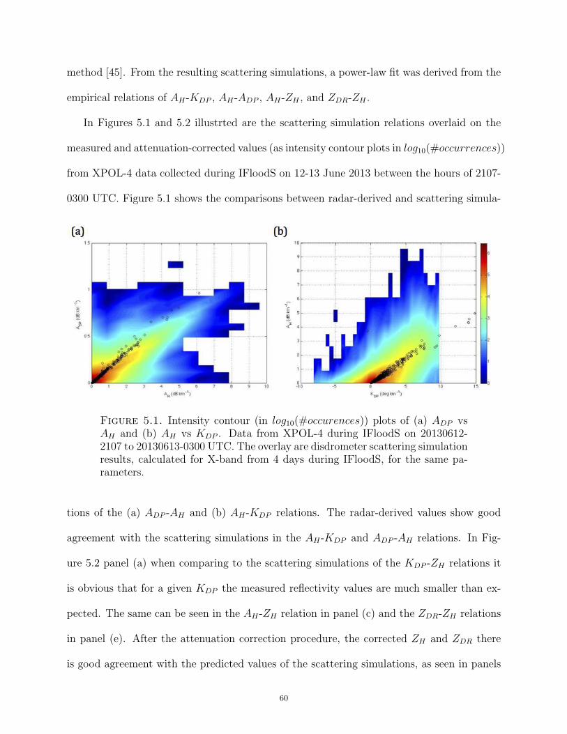
method [45]. From the resulting scattering simulations, a power-law fit was derived from the

empirical relations of AH-KDP , AH-ADP , AH-ZH , and ZDR-ZH .

In Figures 5.1 and 5.2 illustrted are the scattering simulation relations overlaid on the

measured and attenuation-corrected values (as intensity contour plots in log10(#occurrences))

from XPOL-4 data collected during IFloodS on 12-13 June 2013 between the hours of 2107-

0300 UTC. Figure 5.1 shows the comparisons between radar-derived and scattering simula-

Figure 5.1. Intensity contour (in log10(#occurences)) plots of (a) ADP vsAH and (b) AH vs KDP . Data from XPOL-4 during IFloodS on 20130612-2107 to 20130613-0300 UTC. The overlay are disdrometer scattering simulationresults, calculated for X-band from 4 days during IFloodS, for the same pa-rameters.

tions of the (a) ADP -AH and (b) AH-KDP relations. The radar-derived values show good

agreement with the scattering simulations in the AH-KDP and ADP -AH relations. In Fig-

ure 5.2 panel (a) when comparing to the scattering simulations of the KDP -ZH relations it

is obvious that for a given KDP the measured reflectivity values are much smaller than ex-

pected. The same can be seen in the AH-ZH relation in panel (c) and the ZDR-ZH relations

in panel (e). After the attenuation correction procedure, the corrected ZH and ZDR there

is good agreement with the predicted values of the scattering simulations, as seen in panels

60

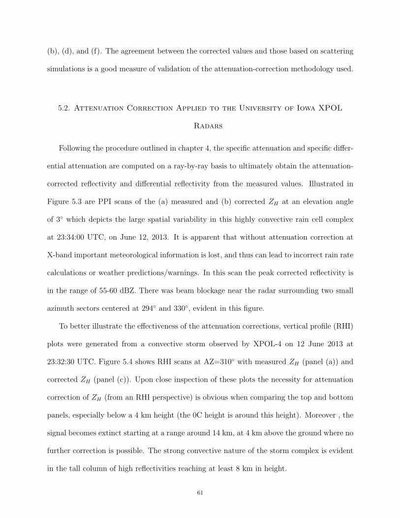
(b), (d), and (f). The agreement between the corrected values and those based on scattering

simulations is a good measure of validation of the attenuation-correction methodology used.

5.2. Attenuation Correction Applied to the University of Iowa XPOL

Radars

Following the procedure outlined in chapter 4, the specific attenuation and specific differ-

ential attenuation are computed on a ray-by-ray basis to ultimately obtain the attenuation-

corrected reflectivity and differential reflectivity from the measured values. Illustrated in

Figure 5.3 are PPI scans of the (a) measured and (b) corrected ZH at an elevation angle

of 3◦ which depicts the large spatial variability in this highly convective rain cell complex

at 23:34:00 UTC, on June 12, 2013. It is apparent that without attenuation correction at

X-band important meteorological information is lost, and thus can lead to incorrect rain rate

calculations or weather predictions/warnings. In this scan the peak corrected reflectivity is

in the range of 55-60 dBZ. There was beam blockage near the radar surrounding two small

azimuth sectors centered at 294◦ and 330◦, evident in this figure.

To better illustrate the effectiveness of the attenuation corrections, vertical profile (RHI)

plots were generated from a convective storm observed by XPOL-4 on 12 June 2013 at

23:32:30 UTC. Figure 5.4 shows RHI scans at AZ=310◦ with measured ZH (panel (a)) and

corrected ZH (panel (c)). Upon close inspection of these plots the necessity for attenuation

correction of ZH (from an RHI perspective) is obvious when comparing the top and bottom

panels, especially below a 4 km height (the 0C height is around this height). Moreover , the

signal becomes extinct starting at a range around 14 km, at 4 km above the ground where no

further correction is possible. The strong convective nature of the storm complex is evident

in the tall column of high reflectivities reaching at least 8 km in height.

61

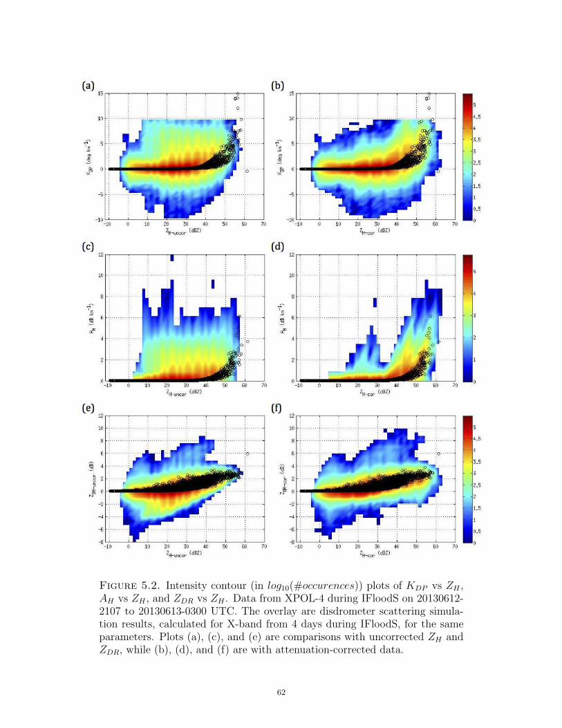
Figure 5.2. Intensity contour (in log10(#occurences)) plots of KDP vs ZH ,AH vs ZH , and ZDR vs ZH . Data from XPOL-4 during IFloodS on 20130612-2107 to 20130613-0300 UTC. The overlay are disdrometer scattering simula-tion results, calculated for X-band from 4 days during IFloodS, for the sameparameters. Plots (a), (c), and (e) are comparisons with uncorrected ZH andZDR, while (b), (d), and (f) are with attenuation-corrected data.

62

Figure 5.3. PPI scans of (a) measured and (b) attenuation-corrected ZH

field from 12 June 2013 at 2334:00 UTC. The origin is at the XPOL-4 radarlocation. The plot axes are aligned with true North/South and West/East,shown with 10 km range rings. The dashed line indicates a vertical RHIprofile at azimuth=10◦.

The measured and corrected ZDR are similarly shown in Figure 5.4 in panels (b) and

(d), respectively. Correction of measured differential reflectivity for differential attenuation

is well illustrated in the vertical by comparing the top and bottom panels. It is difficult to

fully correct for both attenuation and differential attenuation near the melting layer (in the

3.5 - 4 km height interval). This is a region of mixed phase, where in stratiform cells with

a strong bright band we expect melting of larger, low density and dry snowflakes, but in a

convective cell with a weak bright band we anticipate the melting of tiny, compact graupel,

or rimed snow particles [46]. In this vertical profile, we have a convective cell, and thus the

path integrated attenuation (PIA) will be the sum of that due to rain and wet ice, whereas

the propagation phase, ΦDP , is due to the rain component alone, and the backscatter phase,

δ, to the larger drops and/or wet ice. In these situations, a ΦDP constraint is not sufficient

63

Figure 5.4. RHI scans of measured (panels (a) & (b)) and attenuation-corrected (panels (c) & (d)) ZH and ZDR

along the AZ=310◦, from XPOL-4 radar data during IFloodS on June 12, 2013 at 2332:30 UTC, at AZ=310◦.The dashed line indicates the ray profile at an EL=10.7◦

64

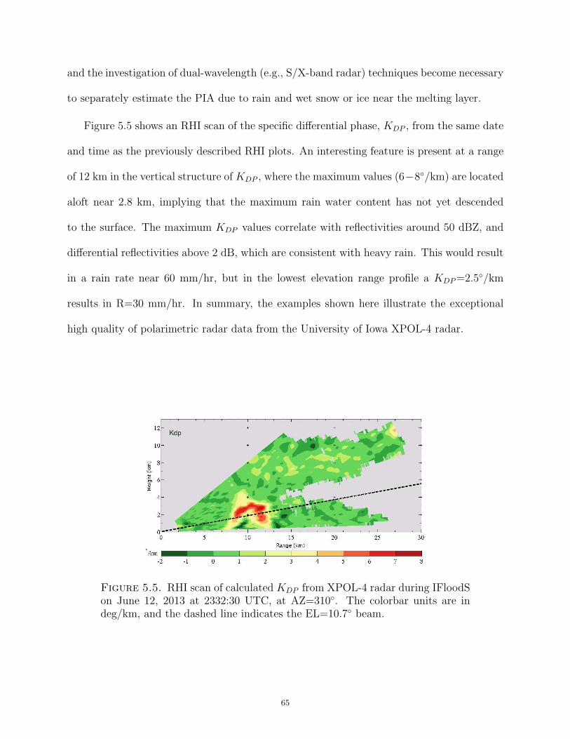
and the investigation of dual-wavelength (e.g., S/X-band radar) techniques become necessary

to separately estimate the PIA due to rain and wet snow or ice near the melting layer.

Figure 5.5 shows an RHI scan of the specific differential phase, KDP , from the same date

and time as the previously described RHI plots. An interesting feature is present at a range

of 12 km in the vertical structure of KDP , where the maximum values (6−8◦/km) are located

aloft near 2.8 km, implying that the maximum rain water content has not yet descended

to the surface. The maximum KDP values correlate with reflectivities around 50 dBZ, and

differential reflectivities above 2 dB, which are consistent with heavy rain. This would result

in a rain rate near 60 mm/hr, but in the lowest elevation range profile a KDP=2.5◦/km

results in R=30 mm/hr. In summary, the examples shown here illustrate the exceptional

high quality of polarimetric radar data from the University of Iowa XPOL-4 radar.

Figure 5.5. RHI scan of calculated KDP from XPOL-4 radar during IFloodSon June 12, 2013 at 2332:30 UTC, at AZ=310◦. The colorbar units are indeg/km, and the dashed line indicates the EL=10.7◦ beam.

65

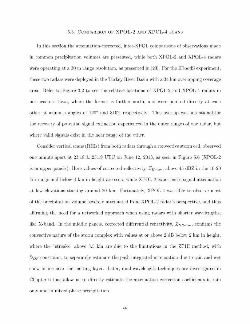
5.3. Comparison of XPOL-2 and XPOL-4 scans

In this section the attenuation-corrected, inter-XPOL comparisons of observations made

in common precipitation volumes are presented, while both XPOL-2 and XPOL-4 radars

were operating at a 30 m range resolution, as presented in [23]. For the IFloodS experiment,

these two radars were deployed in the Turkey River Basin with a 34 km overlapping coverage

area. Refer to Figure 3.2 to see the relative locations of XPOL-2 and XPOL-4 radars in

northeastern Iowa, where the former is further north, and were pointed directly at each

other at azimuth angles of 120o and 310o, respectively. This overlap was intentional for

the recovery of potential signal extinction experienced in the outer ranges of one radar, but

where valid signals exist in the near range of the other.

Consider vertical scans (RHIs) from both radars through a convective storm cell, observed

one minute apart at 23:18 & 23:19 UTC on June 12, 2013, as seen in Figure 5.6 (XPOL-2

is in upper panels). Here values of corrected reflectivity, ZH−cor, above 45 dBZ in the 10-20

km range and below 4 km in height are seen, while XPOL-2 experiences signal attenuation

at low elevations starting around 20 km. Fortunately, XPOL-4 was able to observe most

of the precipitation volume severely attenuated from XPOL-2 radar’s perspective, and thus

affirming the need for a networked approach when using radars with shorter wavelengths,

like X-band. In the middle panels, corrected differential reflectivity, ZDR−cor, confirms the

convective nature of the storm complex with values at or above 2 dB below 2 km in height,

where the ”streaks” above 3.5 km are due to the limitations in the ZPHI method, with

ΦDP constraint, to separately estimate the path integrated attenuation due to rain and wet

snow or ice near the melting layer. Later, dual-wavelength techniques are investigated in

Chapter 6 that allow us to directly estimate the attenuation correction coefficients in rain

only and in mixed-phase precipitation.

66

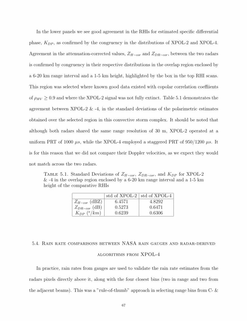
In the lower panels we see good agreement in the RHIs for estimated specific differential

phase, KDP , as confirmed by the congruency in the distributions of XPOL-2 and XPOL-4.

Agreement in the attenuation-corrected values, ZH−cor and ZDR−cor, between the two radars

is confirmed by congruency in their respective distributions in the overlap region enclosed by

a 6-20 km range interval and a 1-5 km height, highlighted by the box in the top RHI scans.

This region was selected where known good data existed with copolar correlation coeffiients

of ρHV ≥ 0.9 and where the XPOL-2 signal was not fully extinct. Table 5.1 demonstrates the

agreement between XPOL-2 & -4, in the standard deviations of the polarimetric estimates

obtained over the selected region in this convective storm complex. It should be noted that

although both radars shared the same range resolution of 30 m, XPOL-2 operated at a

uniform PRT of 1000 µs, while the XPOL-4 employed a staggered PRT of 950/1200 µs. It

is for this reason that we did not compare their Doppler velocities, as we expect they would

not match across the two radars.

Table 5.1. Standard Deviations of ZH−cor, ZDR−cor, and KDP for XPOL-2& -4 in the overlap region enclosed by a 6-20 km range interval and a 1-5 kmheight of the comparative RHIs

std of XPOL-2 std of XPOL-4ZH−cor (dBZ) 6.4571 4.8292ZDR−cor (dB) 0.5273 0.6471KDP (o/km) 0.6239 0.6306

5.4. Rain rate comparisons between NASA rain gauges and radar-derived

algorithms from XPOL-4

In practice, rain rates from gauges are used to validate the rain rate estimates from the

radars pixels directly above it, along with the four closest bins (two in range and two from

the adjacent beams). This was a ”rule-of-thumb” approach in selecting range bins from C- &

67

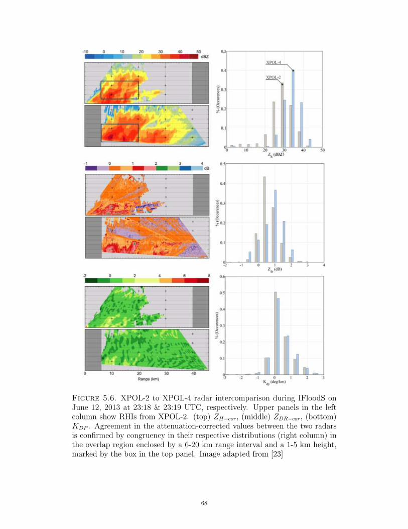
Figure 5.6. XPOL-2 to XPOL-4 radar intercomparison during IFloodS onJune 12, 2013 at 23:18 & 23:19 UTC, respectively. Upper panels in the leftcolumn show RHIs from XPOL-2. (top) ZH−cor, (middle) ZDR−cor, (bottom)KDP . Agreement in the attenuation-corrected values between the two radarsis confirmed by congruency in their respective distributions (right column) inthe overlap region enclosed by a 6-20 km range interval and a 1-5 km height,marked by the box in the top panel. Image adapted from [23]

68

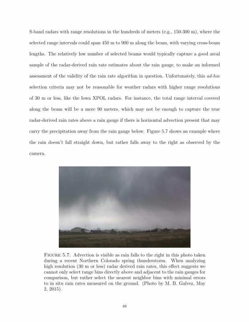
S-band radars with range resolutions in the hundreds of meters (e.g., 150-300 m), where the

selected range intervals could span 450 m to 900 m along the beam, with varying cross-beam

lengths. The relatively low number of selected beams would typically capture a good areal

sample of the radar-derived rain rate estimates about the rain gauge, to make an informed

assessment of the validity of the rain rate algorithm in question. Unfortunately, this ad-hoc

selection criteria may not be reasonable for weather radars with higher range resolutions

of 30 m or less, like the Iowa XPOL radars. For instance, the total range interval covered

along the beam will be a mere 90 meters, which may not be enough to capture the true

radar-derived rain rates above a rain gauge if there is horizontal advection present that may

carry the precipitation away from the rain gauge below. Figure 5.7 shows an example where

the rain doesn’t fall straight down, but rather falls away to the right as observed by the

camera.

Figure 5.7. Advection is visible as rain falls to the right in this photo takenduring a recent Northern Colorado spring thunderstorm. When analyzinghigh resolution (30 m or less) radar derived rain rates, this effect suggests wecannot only select range bins directly above and adjacent to the rain gauges forcomparison, but rather select the nearest neighbor bins with minimal errorsto in situ rain rates measured on the ground. (Photo by M. B. Galvez, May2, 2015).

69

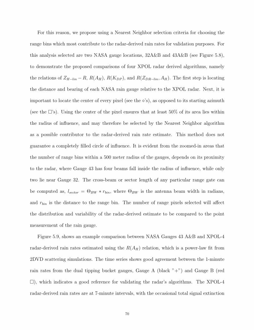
For this reason, we propose using a Nearest Neighbor selection criteria for choosing the

range bins which most contribute to the radar-derived rain rates for validation purposes. For

this analysis selected are two NASA gauge locations, 32A&B and 43A&B (see Figure 5.8),

to demonstrate the proposed comparisons of four XPOL radar derived algorithms, namely

the relations of ZH−lin −R, R(AH), R(KDP ), and R(ZDR−lin, AH). The first step is locating

the distance and bearing of each NASA rain gauge relative to the XPOL radar. Next, it is

important to locate the center of every pixel (see the ⋄’s), as opposed to its starting azimuth

(see the �’s). Using the center of the pixel ensures that at least 50% of its area lies within

the radius of influence, and may therefore be selected by the Nearest Neighbor algorithm

as a possible contributor to the radar-derived rain rate estimate. This method does not

guarantee a completely filled circle of influence. It is evident from the zoomed-in areas that

the number of range bins within a 500 meter radius of the gauges, depends on its proximity

to the radar, where Gauge 43 has four beams fall inside the radius of influence, while only

two lie near Gauge 32. The cross-beam or sector length of any particular range gate can

be computed as, lsector = ΘBW ∗ rbin, where ΘBW is the antenna beam width in radians,

and rbin is the distance to the range bin. The number of range pixels selected will affect

the distribution and variability of the radar-derived estimate to be compared to the point

measurement of the rain gauge.

Figure 5.9, shows an example comparison between NASA Gauges 43 A&B and XPOL-4

radar-derived rain rates estimated using the R(AH) relation, which is a power-law fit from

2DVD scattering simulations. The time series shows good agreement between the 1-minute

rain rates from the dual tipping bucket gauges, Gauge A (black ”+”) and Gauge B (red

�), which indicates a good reference for validating the radar’s algorithms. The XPOL-4

radar-derived rain rates are at 7-minute intervals, with the occasional total signal extinction

70

Figure 5.8. XPOL-4 ZH−cor PPI plot of an inbound convective storm, high-lighting the locations of 12 NASA dual tipping rain gauges within its 40 kmunambiguous range. A blow-up is shown for Gauges 32 and 43, which areused to illustrate the nearest-neighbor selection criteria for range bins withina radius rnn < 500m of the gauges. The �’s represent the starting azimuthof the range bin, and the ⋄’s the center of the bin. Radar data from XPOL-4during IFloodS on 20130612-2334 UTC.

due to high ZH−cor > 55 dBZ, like at 23:53 UTC, as verified in Figure 5.10. In the time

series, radar-derived rain rates are represented with slim filled box plots (in blue) to provide

a sense of the distribution of the nearest neighbors, within a 500 m radius of the NASA A&B

gauges. The box pots show the maximum, minimum, median (circle with a dot), the 75th

and 25th percentiles (top and bottom of filled box), as well as any points considered outliers

of the distribution. Also highlighted on each box plot is the range bin, or pixel, nearest to

the location of the rain gauge (blue ⋄) on the ground below. Each gauge is installed at a

point on the ground and its location is a straight-line distance from the radar, while the

71

individual radar data range bins are actually volumetric representations (enclosed by the

1x1 degree beamwidth of the antenna) at a height above the ground, with respect to the

radar antenna height. Because of the finite fall velocities, there will be some time delay -

of a few minutes - from the radar pixel height to ground level where the gauges are located

(for details on computing fall velocities, see Thurai and Bringi’s section 10.5 in [8]).

Figures 5.11 and 5.12 show the variability in radar-derived rain rates, from the four rain

rate algorithms previously mentioned. In the comparisons to both gauges (32 & 43), it is clear

that estimates derived using R(KDP ) and R(AH) show good agreement with the ground-

based measurements, while the Z-R and R(ZDR, AH) estimates under- or over-estimated rain

rates, respectively. It should be noted that although the R(ZDR, AH) algorithm showed the

least variability in the scattering simulations (see Figure 3.12), it is the most susceptible to

measurement and attenuation-correction errors in ZDR−cor, as evident in the computed over

estimates. The Z-R algorithm made good estimates in low rain rates, and could be used

in a composite rain rate algorithm where estimates of moderate to high rain rates can be

derived from R(KDP ) or R(AH). It should be noted in various of the rain rate algorithm

comparisons, the bin nearest to the gauge (blue ⋄) was well outside the 75%- and 25%-iles

of the values estimated from pixels within the 500m radius of influence, that were close to

the gauge measurements. This provides evidence of the effects due to advection, and for the

need of a nearest-neighbor selection criteria of pixels in radar-derived to rain gauge rain rate

comparisons, for radars operating at high spatio-temporal resolutions.

72

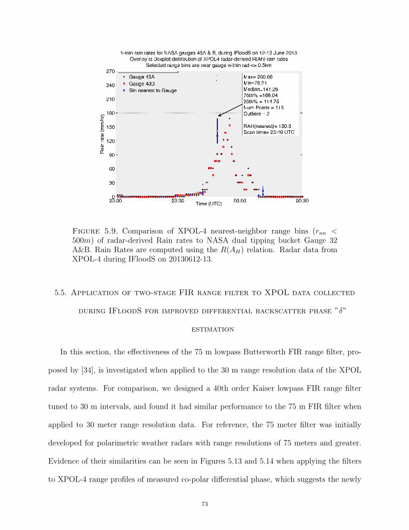
Figure 5.9. Comparison of XPOL-4 nearest-neighbor range bins (rnn <500m) of radar-derived Rain rates to NASA dual tipping bucket Gauge 32A&B. Rain Rates are computed using the R(AH) relation. Radar data fromXPOL-4 during IFloodS on 20130612-13.

5.5. Application of two-stage FIR range filter to XPOL data collected

during IFloodS for improved differential backscatter phase ”δ”

estimation

In this section, the effectiveness of the 75 m lowpass Butterworth FIR range filter, pro-

posed by [34], is investigated when applied to the 30 m range resolution data of the XPOL

radar systems. For comparison, we designed a 40th order Kaiser lowpass FIR range filter

tuned to 30 m intervals, and found it had similar performance to the 75 m FIR filter when

applied to 30 meter range resolution data. For reference, the 75 meter filter was initially

developed for polarimetric weather radars with range resolutions of 75 meters and greater.

Evidence of their similarities can be seen in Figures 5.13 and 5.14 when applying the filters

to XPOL-4 range profiles of measured co-polar differential phase, which suggests the newly

73

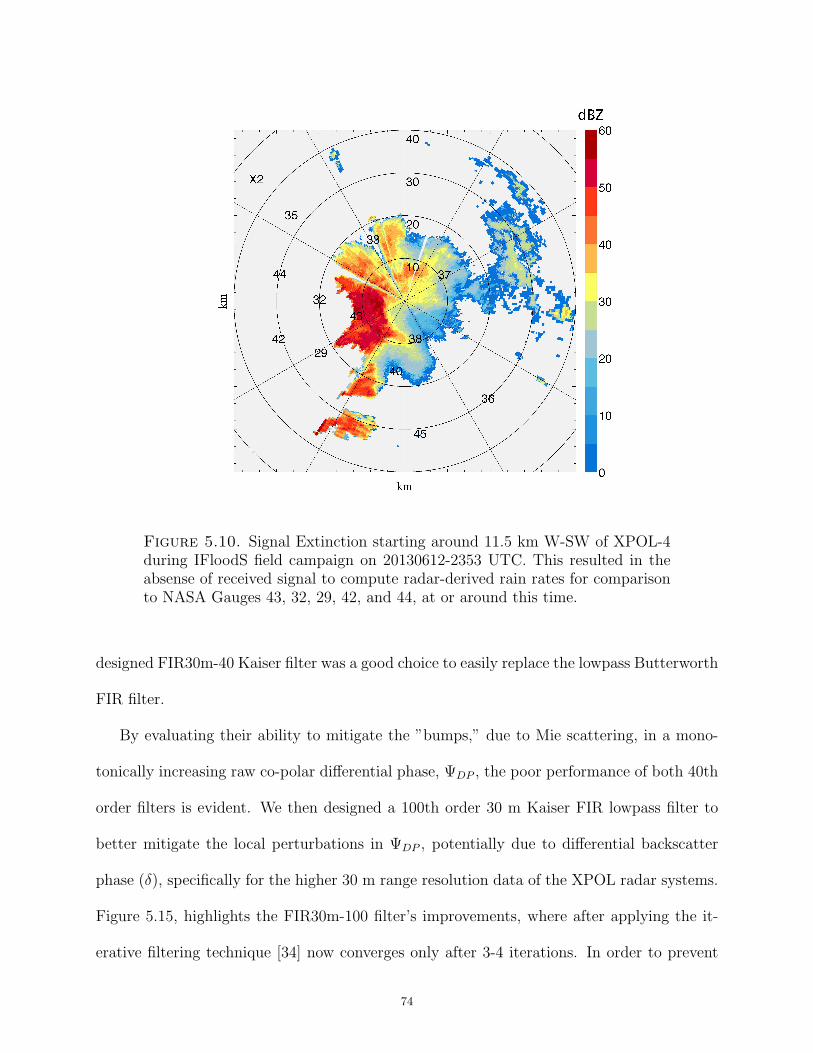
Figure 5.10. Signal Extinction starting around 11.5 km W-SW of XPOL-4during IFloodS field campaign on 20130612-2353 UTC. This resulted in theabsense of received signal to compute radar-derived rain rates for comparisonto NASA Gauges 43, 32, 29, 42, and 44, at or around this time.

designed FIR30m-40 Kaiser filter was a good choice to easily replace the lowpass Butterworth

FIR filter.

By evaluating their ability to mitigate the ”bumps,” due to Mie scattering, in a mono-

tonically increasing raw co-polar differential phase, ΨDP , the poor performance of both 40th

order filters is evident. We then designed a 100th order 30 m Kaiser FIR lowpass filter to

better mitigate the local perturbations in ΨDP , potentially due to differential backscatter

phase (δ), specifically for the higher 30 m range resolution data of the XPOL radar systems.

Figure 5.15, highlights the FIR30m-100 filter’s improvements, where after applying the it-

erative filtering technique [34] now converges only after 3-4 iterations. In order to prevent

74

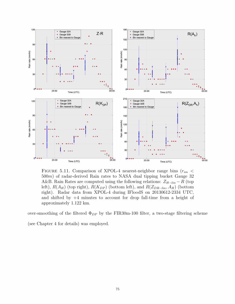
Figure 5.11. Comparison of XPOL-4 nearest-neighbor range bins (rnn <500m) of radar-derived Rain rates to NASA dual tipping bucket Gauge 32A&B. Rain Rates are computed using the following relations: ZH−lin−R (topleft), R(AH) (top right), R(KDP ) (bottom left), and R(ZDR−lin, AH) (bottomright). Radar data from XPOL-4 during IFloodS on 20130612-2334 UTC,and shifted by +4 minutes to account for drop fall-time from a height ofapproximately 1.122 km.

over-smoothing of the filtered ΦDP by the FIR30m-100 filter, a two-stage filtering scheme

(see Chapter 4 for details) was employed.

75

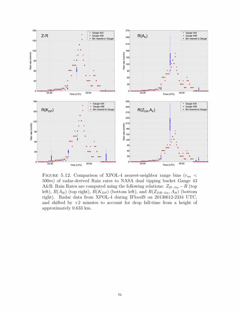
Figure 5.12. Comparison of XPOL-4 nearest-neighbor range bins (rnn <500m) of radar-derived Rain rates to NASA dual tipping bucket Gauge 43A&B. Rain Rates are computed using the following relations: ZH−lin−R (topleft), R(AH) (top right), R(KDP ) (bottom left), and R(ZDR−lin, AH) (bottomright). Radar data from XPOL-4 during IFloodS on 20130612-2334 UTC,and shifted by +2 minutes to account for drop fall-time from a height ofapproximately 0.633 km.

76

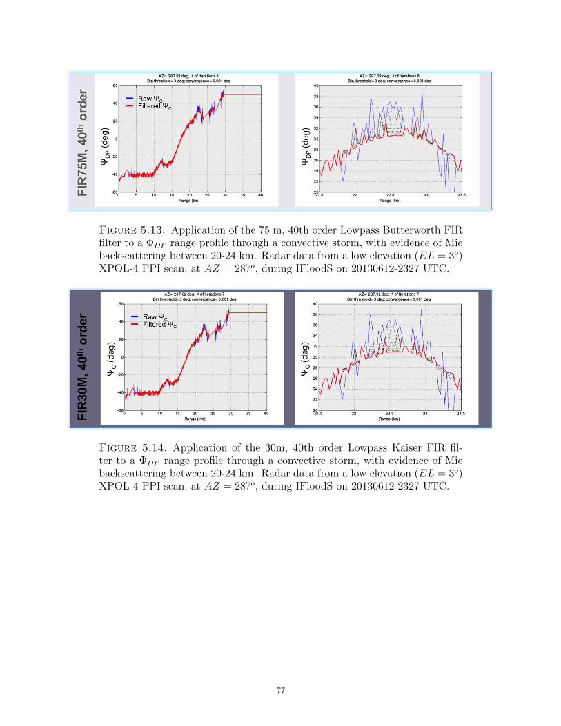
Figure 5.13. Application of the 75 m, 40th order Lowpass Butterworth FIRfilter to a ΦDP range profile through a convective storm, with evidence of Miebackscattering between 20-24 km. Radar data from a low elevation (EL = 3o)XPOL-4 PPI scan, at AZ = 287o, during IFloodS on 20130612-2327 UTC.

Figure 5.14. Application of the 30m, 40th order Lowpass Kaiser FIR fil-ter to a ΦDP range profile through a convective storm, with evidence of Miebackscattering between 20-24 km. Radar data from a low elevation (EL = 3o)XPOL-4 PPI scan, at AZ = 287o, during IFloodS on 20130612-2327 UTC.

77

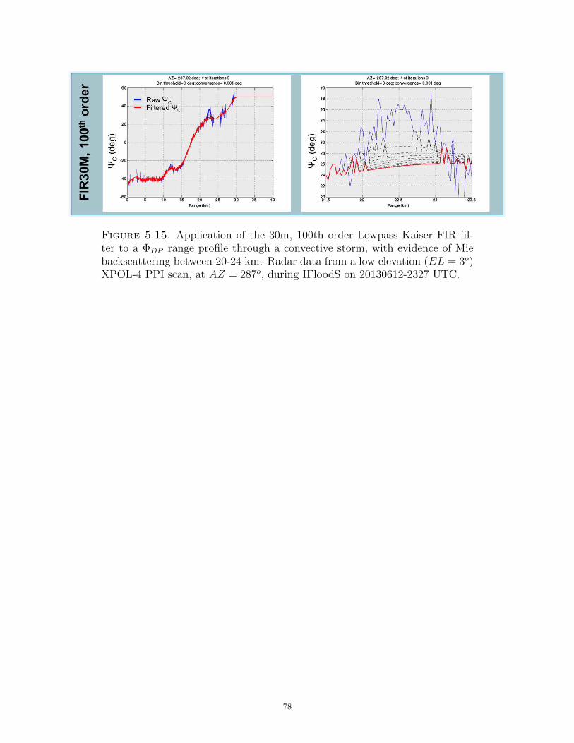
Figure 5.15. Application of the 30m, 100th order Lowpass Kaiser FIR fil-ter to a ΦDP range profile through a convective storm, with evidence of Miebackscattering between 20-24 km. Radar data from a low elevation (EL = 3o)XPOL-4 PPI scan, at AZ = 287o, during IFloodS on 20130612-2327 UTC.

78

CHAPTER 6

Dual Wavelength Ratios of Reflectivity &

Differential Reflectivity

The accuracy of dual-wavelength techniques depend on proper matching of the S- and

X-band radar beam resolution in azimuth, elevation, radial range spacing, and timing of

the pulse triggering between the two systems. As described in Chapter 2, the CHILL S/X-

band radar signals share the same antenna, although with 1 deg beamwidth at S-band and

about 0.3 deg at X-band with a higher gain. For the analysis herein we synthesize the

higher resolution X-band beam width to match the S-band beam, with an approximately 3:1

beam ratio (X:S). Aside from hail detection, the dual-wavelength ratio allows for using the

virtually unattenuated S-band reflectivity measurement as a constraint in the attenuation

correction algorithm that can be applied directly to the measured X-band data. We focus

on the attenuation correction aspect of the dual-wavelength ratios and the variability of the

α & β coefficients with height, in rain-only, and in rain/hail mixtures.

6.1. Description of Dual Wavelength Analysis Procedure

We investigate dual-wavelength algorithms to directly estimate the α and β coefficients,

of the AH = αKDP and ADP = βKDP relations, to obtain the path integrated attenuation

due to rain and wet ice or snow in the region near the melting layer. We use data from the

dual-wavelength, dual-polarization CHILL S-/X-band Doppler weather radar for analyzing

the coefficients and compare their variability as a function of height, where the hydrometeors

are expected to go through a microphysical transformation as they fall, starting as snow or

graupel/hail then melting into rain or a rain-hail mixture. The S-band signal is un-attenuated

79

and so forms a reference for estimating the X-band attenuation and differential attenuation.

We present the ranges of the α and β coefficients in these varying precipitation regimes

to help improve KDP-based attenuation correction algorithms at X-band as well as rain

rate algorithms based on the derived specific attenuation, AH . One such rainfall estimation

algorithm, R(AH), was presented by [19] and tested at X-band to include mitigation of

partial beam blockage and also in a networked radar configuration.

Figure 6.1 shows RHI scans of reflectivity at (a) S-band ZH−S and (c) X-band, ZH−X ,

and their corresponding differential reflectivities (b) ZDR−S and (d) ZDR−X observed by the

CSU-CHILL S/X-band radar at an azimuth angle of 291◦. These scans were through a mostly

rain-only event observed on 18 July 2013 at 22:10 UTC, and was previously identified as such

in a study presented by [7]. We can see reflectivity values greater than 40 dBZ at heights

at or above 3 km in both reflectivity plots, while it is evident how the effects of attenuation

diminish ZH−X beyond 30 km in range, as it propagates through the heavier rainfall. The

effects of attenuation on ZDR−X are apparent in the image as the ”negative ZDR shadow”

cast beyond 30 km range, due to ZH attenuating more than ZV (where ZDR = ZH −ZV ), as

the pulse propagates through a medium composed of larger oblate rain drops. It is in these

regions of attenuation at X-band that we can directly estimate the coefficients and correct for

specific and differential attenuation from the AH = αKDP−X and ADP = βKDP−X relations.

To demonstrate the application of the dual-wavelength procedure, we select a beam that

propagates through rain only, and below the melting layer, so we consider the range profile

at an elevation of 1.7◦, as highlighted by the black line in the RHIs. We estimate the α

and β coefficients directly from the dual-wavelength equations( 2.19) and (2.20) defined in

Chapter 2. Figure 6.3 shows range profiles of (a) ZH−S and ZH−X vs ΦDP−X , (b) ZDR−S

80

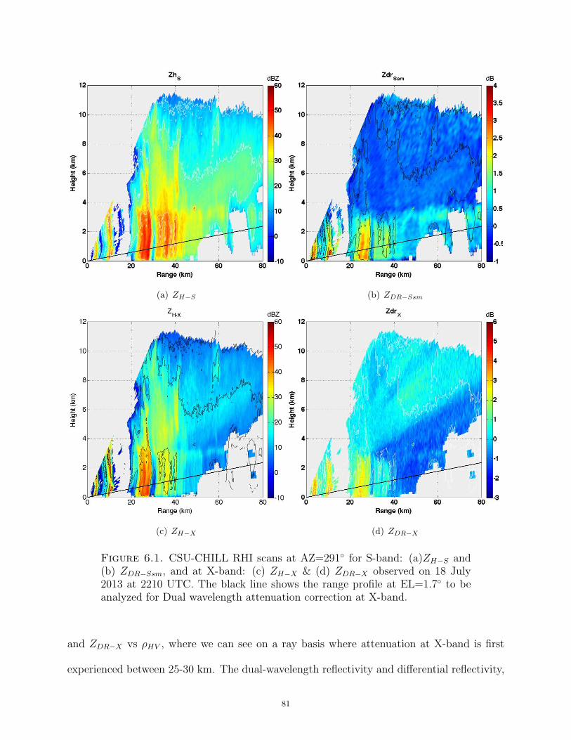
(a) ZH−S (b) ZDR−Ssm

(c) ZH−X (d) ZDR−X

Figure 6.1. CSU-CHILL RHI scans at AZ=291◦ for S-band: (a)ZH−S and(b) ZDR−Ssm, and at X-band: (c) ZH−X & (d) ZDR−X observed on 18 July2013 at 2210 UTC. The black line shows the range profile at EL=1.7◦ to beanalyzed for Dual wavelength attenuation correction at X-band.

and ZDR−X vs ρHV , where we can see on a ray basis where attenuation at X-band is first

experienced between 25-30 km. The dual-wavelength reflectivity and differential reflectivity,

81

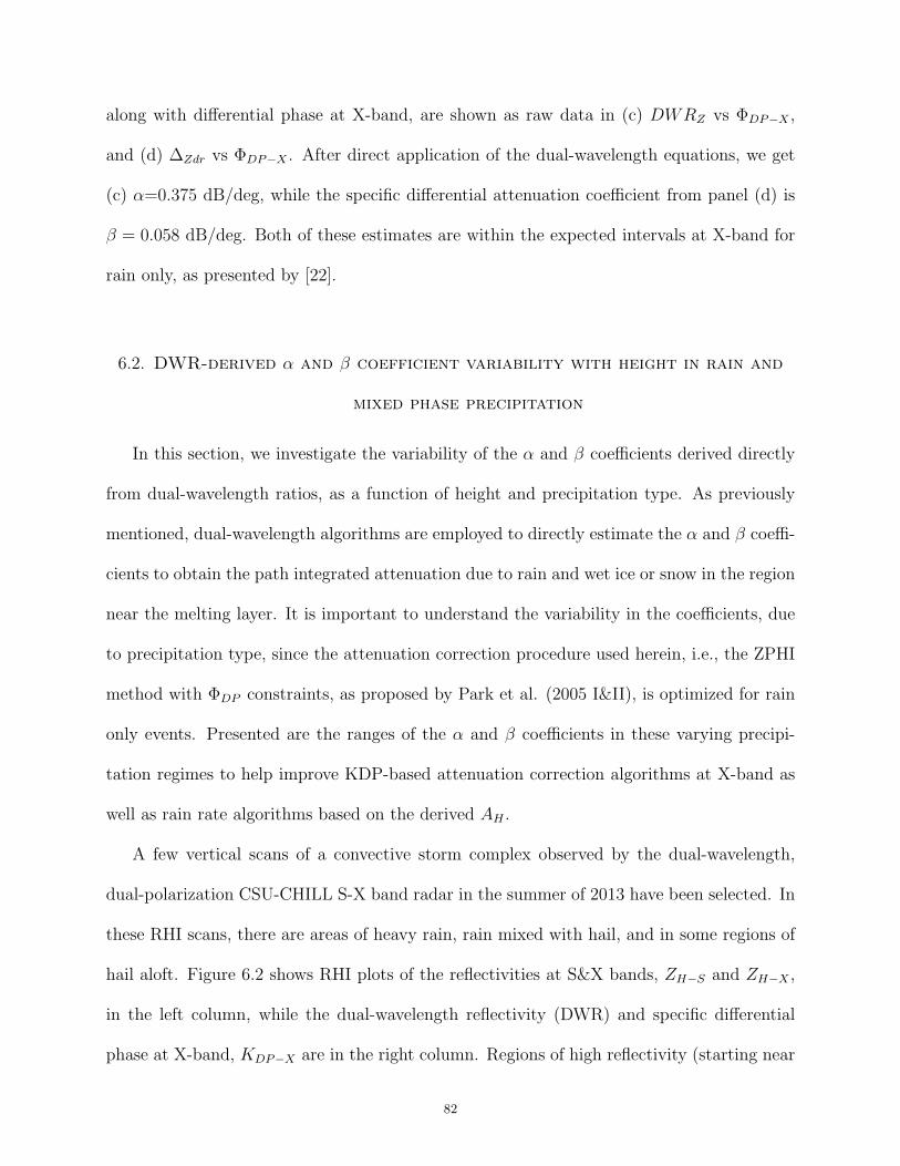
along with differential phase at X-band, are shown as raw data in (c) DWRZ vs ΦDP−X ,

and (d) ∆Zdr vs ΦDP−X . After direct application of the dual-wavelength equations, we get

(c) α=0.375 dB/deg, while the specific differential attenuation coefficient from panel (d) is

β = 0.058 dB/deg. Both of these estimates are within the expected intervals at X-band for

rain only, as presented by [22].

6.2. DWR-derived α and β coefficient variability with height in rain and

mixed phase precipitation

In this section, we investigate the variability of the α and β coefficients derived directly

from dual-wavelength ratios, as a function of height and precipitation type. As previously

mentioned, dual-wavelength algorithms are employed to directly estimate the α and β coeffi-

cients to obtain the path integrated attenuation due to rain and wet ice or snow in the region

near the melting layer. It is important to understand the variability in the coefficients, due

to precipitation type, since the attenuation correction procedure used herein, i.e., the ZPHI

method with ΦDP constraints, as proposed by Park et al. (2005 I&II), is optimized for rain

only events. Presented are the ranges of the α and β coefficients in these varying precipi-

tation regimes to help improve KDP-based attenuation correction algorithms at X-band as

well as rain rate algorithms based on the derived AH .

A few vertical scans of a convective storm complex observed by the dual-wavelength,

dual-polarization CSU-CHILL S-X band radar in the summer of 2013 have been selected. In

these RHI scans, there are areas of heavy rain, rain mixed with hail, and in some regions of

hail aloft. Figure 6.2 shows RHI plots of the reflectivities at S&X bands, ZH−S and ZH−X ,

in the left column, while the dual-wavelength reflectivity (DWR) and specific differential

phase at X-band, KDP−X are in the right column. Regions of high reflectivity (starting near

82

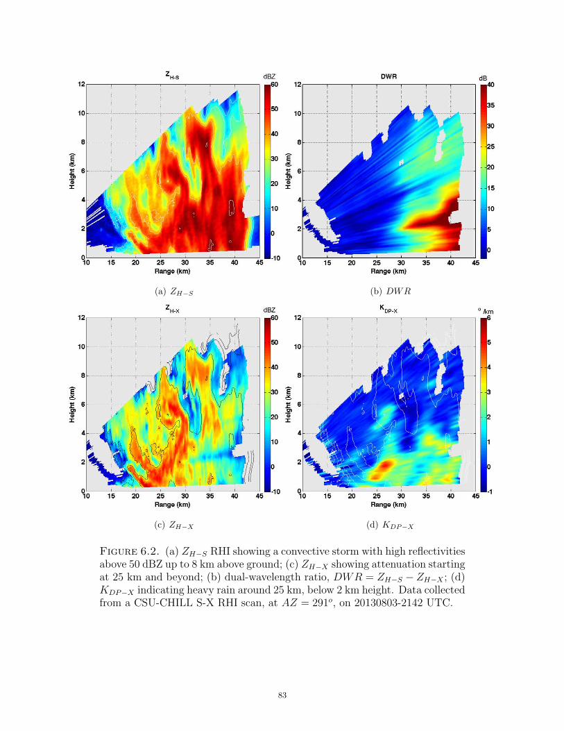
(a) ZH−S (b) DWR

(c) ZH−X (d) KDP−X

Figure 6.2. (a) ZH−S RHI showing a convective storm with high reflectivitiesabove 50 dBZ up to 8 km above ground; (c) ZH−X showing attenuation startingat 25 km and beyond; (b) dual-wavelength ratio, DWR = ZH−S − ZH−X ; (d)KDP−X indicating heavy rain around 25 km, below 2 km height. Data collectedfrom a CSU-CHILL S-X RHI scan, at AZ = 291o, on 20130803-2142 UTC.

83

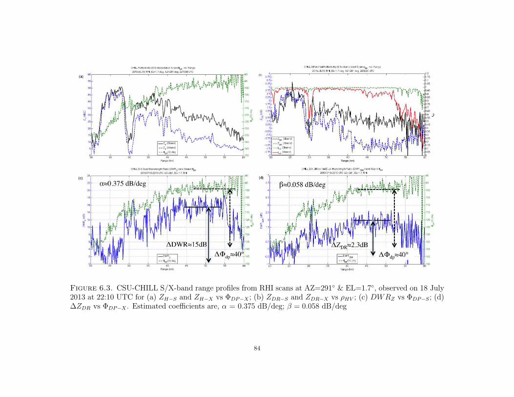
Figure 6.3. CSU-CHILL S/X-band range profiles from RHI scans at AZ=291◦ & EL=1.7◦, observed on 18 July2013 at 22:10 UTC for (a) ZH−S and ZH−X vs ΦDP−X ; (b) ZDR−S and ZDR−X vs ρHV ; (c) DWRZ vs ΦDP−S; (d)∆ZDR vs ΦDP−X . Estimated coefficients are, α = 0.375 dB/deg; β = 0.058 dB/deg

84

30 km in radial range) are evident in the ZH−S plot, and the rapidly attenuating signal

in the ZH−X plot. The dual-wavelength reflectivity shows the degree of accumulating path

integrated attenuation as the beams propagate through the volumes filled with larger oblate

hydrometeors, with peak attenuation beyond 30 km and above 2.5 km in height. We take

advantage of the more sensitive differential propagation phase at X-band, which is immune

to the effects of attenuation (unless the signal is extinct), to detect areas of heavy rainfall

like that seen around 25 km in range. From these RHIs, coupled with the computed Hail

Detection Ratio (HDR, not shown) we were able to identify regions of uniform rain (25-30

km), as well as rain-hail mix and hail aloft regions (30-35 km) for analysis of the variability

in α and β with height, and through the different precipitation regimes.

6.2.1. Dual-Wavelength derived α coefficient in uniform Rain and Rain-

Hail mixed phase regions. First, the α coefficient is computed in ”rain-only” regions

between the range interval of 25-30 km, applying the dual-wavelength technique previously

described. In Figure 6.4, we show the vertical profiles, averaged over the range interval

(25-30km), of reflectivity and differential reflectivity at S-band, ZH−S & ZDR−S, along with

those for specific attenuation and specific differential phase at X-band, AH−X and KDP−X .

This indeed is a heavy rainfall with high reflectivities and positive ZDR−S values seen up

to 5.5 km. The relatively low Mie signal (upper right panel) below 5 km height indicates

the absence of melting snow/hail which could lead to the presence of differential backscatter

phase signal. The α-vs-height profile is that for a purely rain only event below 3 km, with

values near that computed from 2DVD scattering simulations, at α ≈ 0.3 dB/deg. There is

good agreement between the α = AH−X/KDP−X relation in the vertical profile and the dual-

wavelength derived α coefficient as a function of height. This behavior of increasing α with

85

height is expected as we get into regions of mixed phase where wet quasi-spherical frozen

particles produce a lower ΦDP−X , positively biasing the inversely proportional coefficient.

Figure 6.4. α vs. height in Rain-only. (left) Vertical profiles, betweenrange=25-30 km, of ZH−S, ZDR−S, AH−X , and KDP−X from a CHILL S-XRHI scan, at AZ = 291o, on 20130803-2142 UTC; (top right) low Mie scat-ter signal over the range interval; (bottom right) α coefficient estimated, overthe range interval between 25-30 km on a ray-by-ray basis, using the directα = ∆DWR/∆ΦDP−X method. This was determined to be a ”Rain-only”region below 3 km in height, which was confirmed with α ≈ 0.3dB/deg andthe low Mie signal, as expected.

In Figure 6.5 we consider estimation of the α coefficient in the rain-hail mixed phase range

interval between 30-35 km, showing (left panel) the vertical profiles of ZH−S, ZDR−S, AH−X ,

and KDP−X ; (top right) the Mie signal RHI scan indicating mixed-phase hydrometeors above

3 km; and (bottom right) the DWR-derived α coefficient as a function of height. The radar

data used for this ananlysis is from a CSU-CHILL S-X RHI scan, at AZ = 291o, as observed

86

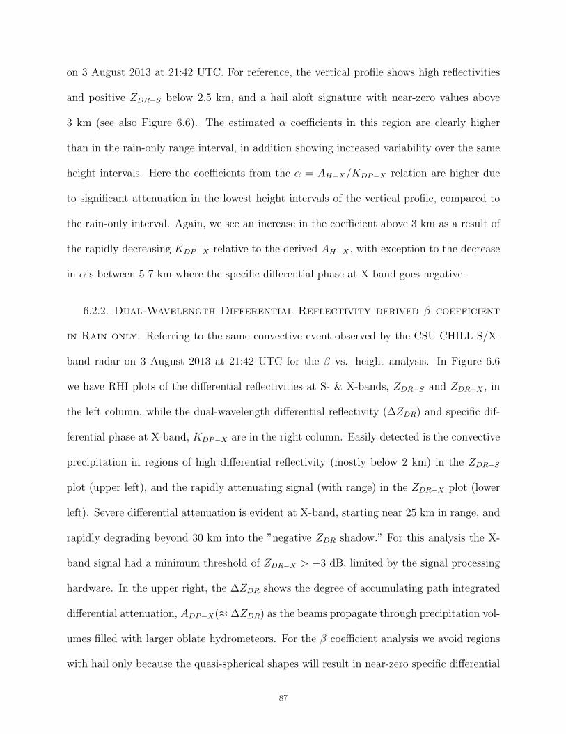
on 3 August 2013 at 21:42 UTC. For reference, the vertical profile shows high reflectivities

and positive ZDR−S below 2.5 km, and a hail aloft signature with near-zero values above

3 km (see also Figure 6.6). The estimated α coefficients in this region are clearly higher

than in the rain-only range interval, in addition showing increased variability over the same

height intervals. Here the coefficients from the α = AH−X/KDP−X relation are higher due

to significant attenuation in the lowest height intervals of the vertical profile, compared to

the rain-only interval. Again, we see an increase in the coefficient above 3 km as a result of

the rapidly decreasing KDP−X relative to the derived AH−X , with exception to the decrease

in α’s between 5-7 km where the specific differential phase at X-band goes negative.

6.2.2. Dual-Wavelength Differential Reflectivity derived β coefficient

in Rain only. Referring to the same convective event observed by the CSU-CHILL S/X-

band radar on 3 August 2013 at 21:42 UTC for the β vs. height analysis. In Figure 6.6

we have RHI plots of the differential reflectivities at S- & X-bands, ZDR−S and ZDR−X , in

the left column, while the dual-wavelength differential reflectivity (∆ZDR) and specific dif-

ferential phase at X-band, KDP−X are in the right column. Easily detected is the convective

precipitation in regions of high differential reflectivity (mostly below 2 km) in the ZDR−S

plot (upper left), and the rapidly attenuating signal (with range) in the ZDR−X plot (lower

left). Severe differential attenuation is evident at X-band, starting near 25 km in range, and

rapidly degrading beyond 30 km into the ”negative ZDR shadow.” For this analysis the X-

band signal had a minimum threshold of ZDR−X > −3 dB, limited by the signal processing

hardware. In the upper right, the ∆ZDR shows the degree of accumulating path integrated

differential attenuation, ADP−X(≈ ∆ZDR) as the beams propagate through precipitation vol-

umes filled with larger oblate hydrometeors. For the β coefficient analysis we avoid regions

with hail only because the quasi-spherical shapes will result in near-zero specific differential

87

Figure 6.5. α vs. height in Rain-Hail mix. (left) Vertical profiles, betweenrange=30-35 km, of ZH−S, ZDR−S, AH−X , and KDP−X from a CSU-CHILLS-X RHI scan, at AZ = 291o, on 20130803-2142 UTC; (top right) high Miescatter signal over the range interval; (bottom right) α coefficient estimated,over the range interval between 30-35 km on a ray-by-ray basis, using the directα = ∆DWR/∆ΦDP−X method. This was determined to be a ”mixed-phase”column, which was confirmed with higher α’s and increasing Mie signal withheight. The vertical profiles show near-zero ZDR−S, with ZH−S ≈ 50 dBZ, anddecreasing KDP−X above 3 km, indicating spherical particles probably due towet hail aloft.

phase at X-band which can cause a singularity in the relation, β ≈ ∆ZDR/∆ΦDP−X . We

focus on the 25-30 km range interval below 5 km, dominated by rain only, and avoid the

mixed phase 30-35 km interval with prevailing hail regions, apparent in the near-zero ZDR−S

column aloft above 2 km.

In Figure 6.7 the estimation of β coefficient in a rain-only range interval between 25-30

km and below 6 km in height is considered, where in the left panel are the vertical profiles

of ZH−S, ZDR−S, ZDR−X , and KDP−X ; (top right) the ∆ZDR signal as an RHI scan; and

88

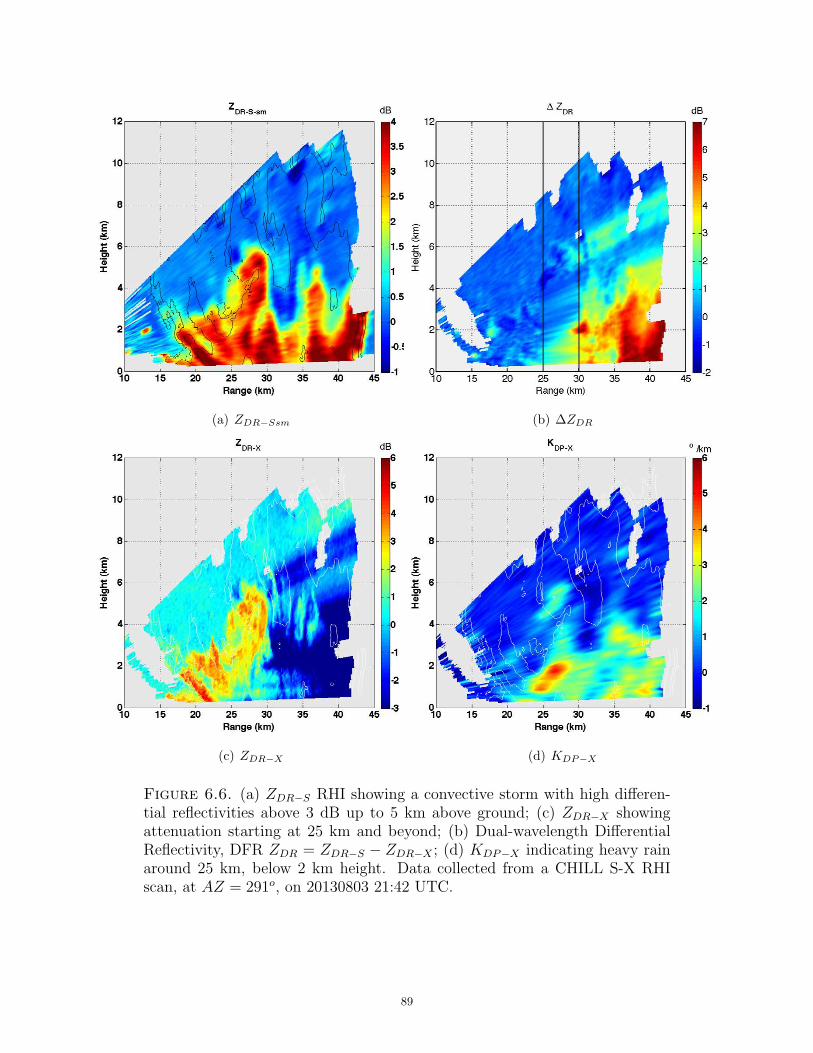
(a) ZDR−Ssm (b) ∆ZDR

(c) ZDR−X (d) KDP−X

Figure 6.6. (a) ZDR−S RHI showing a convective storm with high differen-tial reflectivities above 3 dB up to 5 km above ground; (c) ZDR−X showingattenuation starting at 25 km and beyond; (b) Dual-wavelength DifferentialReflectivity, DFR ZDR = ZDR−S − ZDR−X ; (d) KDP−X indicating heavy rainaround 25 km, below 2 km height. Data collected from a CHILL S-X RHIscan, at AZ = 291o, on 20130803 21:42 UTC.

89

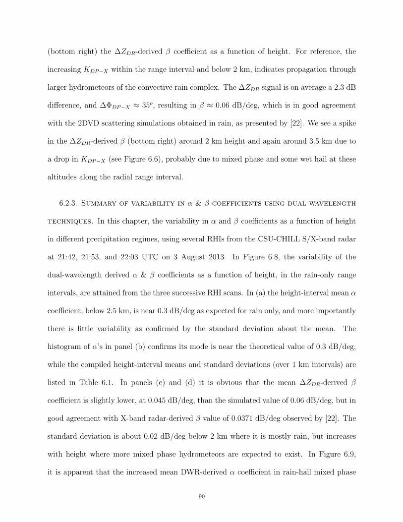
(bottom right) the ∆ZDR-derived β coefficient as a function of height. For reference, the

increasing KDP−X within the range interval and below 2 km, indicates propagation through

larger hydrometeors of the convective rain complex. The ∆ZDR signal is on average a 2.3 dB

difference, and ∆ΦDP−X ≈ 35o, resulting in β ≈ 0.06 dB/deg, which is in good agreement

with the 2DVD scattering simulations obtained in rain, as presented by [22]. We see a spike

in the ∆ZDR-derived β (bottom right) around 2 km height and again around 3.5 km due to

a drop in KDP−X (see Figure 6.6), probably due to mixed phase and some wet hail at these

altitudes along the radial range interval.

6.2.3. Summary of variability in α & β coefficients using dual wavelength

techniques. In this chapter, the variability in α and β coefficients as a function of height

in different precipitation regimes, using several RHIs from the CSU-CHILL S/X-band radar

at 21:42, 21:53, and 22:03 UTC on 3 August 2013. In Figure 6.8, the variability of the

dual-wavelength derived α & β coefficients as a function of height, in the rain-only range

intervals, are attained from the three successive RHI scans. In (a) the height-interval mean α

coefficient, below 2.5 km, is near 0.3 dB/deg as expected for rain only, and more importantly

there is little variability as confirmed by the standard deviation about the mean. The

histogram of α’s in panel (b) confirms its mode is near the theoretical value of 0.3 dB/deg,

while the compiled height-interval means and standard deviations (over 1 km intervals) are

listed in Table 6.1. In panels (c) and (d) it is obvious that the mean ∆ZDR-derived β

coefficient is slightly lower, at 0.045 dB/deg, than the simulated value of 0.06 dB/deg, but in

good agreement with X-band radar-derived β value of 0.0371 dB/deg observed by [22]. The

standard deviation is about 0.02 dB/deg below 2 km where it is mostly rain, but increases

with height where more mixed phase hydrometeors are expected to exist. In Figure 6.9,

it is apparent that the increased mean DWR-derived α coefficient in rain-hail mixed phase

90

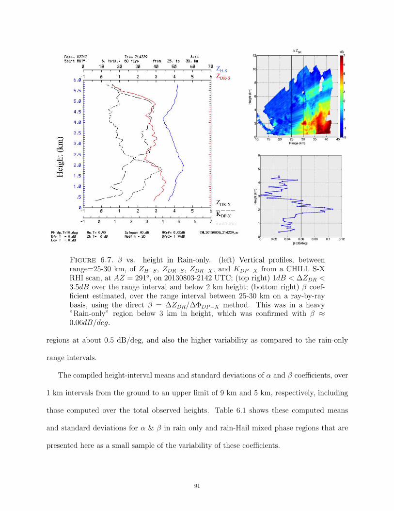
Figure 6.7. β vs. height in Rain-only. (left) Vertical profiles, betweenrange=25-30 km, of ZH−S, ZDR−S, ZDR−X , and KDP−X from a CHILL S-XRHI scan, at AZ = 291o, on 20130803-2142 UTC; (top right) 1dB < ∆ZDR <3.5dB over the range interval and below 2 km height; (bottom right) β coef-ficient estimated, over the range interval between 25-30 km on a ray-by-raybasis, using the direct β = ∆ZDR/∆ΦDP−X method. This was in a heavy”Rain-only” region below 3 km in height, which was confirmed with β ≈0.06dB/deg.

regions at about 0.5 dB/deg, and also the higher variability as compared to the rain-only

range intervals.

The compiled height-interval means and standard deviations of α and β coefficients, over

1 km intervals from the ground to an upper limit of 9 km and 5 km, respectively, including

those computed over the total observed heights. Table 6.1 shows these computed means

and standard deviations for α & β in rain only and rain-Hail mixed phase regions that are

presented here as a small sample of the variability of these coefficients.

91

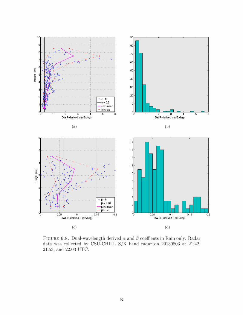
(a) (b)

(c) (d)

Figure 6.8. Dual-wavelength derived α and β coeffients in Rain only. Radardata was collected by CSU-CHILL S/X band radar on 20130803 at 21:42,21:53, and 22:03 UTC.

92

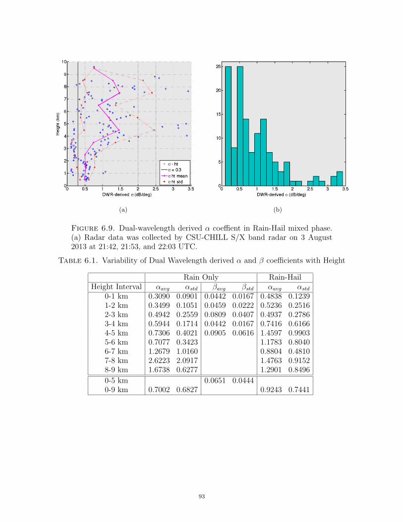
(a) (b)

Figure 6.9. Dual-wavelength derived α coeffient in Rain-Hail mixed phase.(a) Radar data was collected by CSU-CHILL S/X band radar on 3 August2013 at 21:42, 21:53, and 22:03 UTC.

Table 6.1. Variability of Dual Wavelength derived α and β coefficients with Height

Rain Only Rain-HailHeight Interval αavg αstd βavg βstd αavg αstd

0-1 km 0.3090 0.0901 0.0442 0.0167 0.4838 0.12391-2 km 0.3499 0.1051 0.0459 0.0222 0.5236 0.25162-3 km 0.4942 0.2559 0.0809 0.0407 0.4937 0.27863-4 km 0.5944 0.1714 0.0442 0.0167 0.7416 0.61664-5 km 0.7306 0.4021 0.0905 0.0616 1.4597 0.99035-6 km 0.7077 0.3423 1.1783 0.80406-7 km 1.2679 1.0160 0.8804 0.48107-8 km 2.6223 2.0917 1.4763 0.91528-9 km 1.6738 0.6277 1.2901 0.8496

0-5 km 0.0651 0.04440-9 km 0.7002 0.6827 0.9243 0.7441

93

CHAPTER 7

Summary, Conclusions

This body of work has presented the primary objectives of this research and the results,

obtained from data collected during the Iowa Flood Studies (IFloodS) in spring 2013, to

support the proposed solutions. In Chapter 3, we presented the role regional climatology

has on the variability of drop size distributions of 2DVD scattering simulations, relative to

the effects in a global sense. We also presented the effects on scattering-derived alpha and

beta coefficients, of the AH−KDP and ADP −KDP relations, as well as how these coefficients

vary based on regional versus global climatologies. The ranges in alpha and beta coefficients,

extracted from the Global histograms are applicable to coefficient optimization in the it-

erative ZPHI method, with ΦDP constraint. In Chapter 4 we presented the ZPHI method

for attenuation correction, tuned for X-band polarimetric radars with high spatio-temporal

resolution and dedicated to hydrology studies of vast river basins and watersheds. We pro-

posed a new two-stage FIR range filtering technique with improved estimation of differential

backscatter phase, due to Mie scattering effects at X-band, which has implications for more

accurate KDP estimates and related rain rated algorithms. In Chapter 5, we selected the

XPOL radar platform of the Iowa Flood Center, i.e., the four-node transportable X-band

polarimetric radar network dedicated to hydrology studies, for the development and valida-

tion of the modified ZPHI attenuation correction algorithm, and furthermore for validating

the new backscatter differential phase estimator. The results shown herein for the XPOL-4

radar display good agreement between the regional 2DVD scattering simulations and the

attenuation-corrected radar moments (ZH , ZDR, and KDP ) suggesting good quality data

from the applied correction methodology. Although the correction method showed good

94

results for rain-only events, it is difficult to fully correct attenuation near the melting layer

where a mixed phase of rain and melting graupel exists. In Chapter 6 we highlight the ben-

efits of dual-wavelength reflectivity (DWR) and differential reflectivity (∆ZDR) algorithms,

developed with CSU-CHILL S/X-band radar, to directly and separately estimate the path

integrated attenuation due to rain and wet snow/ice in the region near the melting layer.

The DWR and ∆ZDR algorithms were also key in determining the variability in direct mea-

surement estimates of α and β coefficients, as a function of height above the ground and for

different precipitation types.

The research objectives were met, and will compliment the body of knowledge regard-

ing attenuation correction for polarimetric weather radars operating at high spatio-temporal

resolutions in the shorter X-band wavelength regime. Although the results presented herein

proved to be significant improvements to the present readily available X-band polarimetric

technologies, the future of X-band polarimetric weather radars lies in phased-array plat-

forms yielding much faster scan times, thereby making even higher spatio-temporal rain

rate estimates. Phased array radars will need to overcome cost prohibitive barriers, as well

as antenna impurities seen off the beam boresight, that can contribute significant sidelobe

interference.

95

Bibliography

[1] R. J. Doviak and D. S. Zrnic, Doppler Radar and Weather Observations. Academic

Press Inc., 2nd ed., 1993.

[2] V. Bringi and V. Chandrasekaran, Polarimetric Doppler Weather Radar: Principles and

Applications. Cambridge University Press., 2001.

[3] F. Junyent, V. Chandrasekar, V. N. Bringi, S. A. Rutledge, P. C. Kennedy, D. Brunkow,

J. George, and R. Bowie, “Transformation of the CSU–CHILL Radar Facility to a Dual-

Frequency, Dual-Polarization Doppler System,” Bulletin of the American Meteorological

Society, vol. 96, no. 6, pp. 975–996, 2014.

[4] K. V. Mishra, A. Kruger, andW. F. Krajewski, “Engineering Evaluation and Calibration

of Iowa X-Band Polarimetric Radars,” in EGU General Assembly Conference Abstracts,

vol. 15, p. 13010, 2013.

[5] W. F. Krajewski, K. V. Mishra, R. Goska, D. Ceynar, B.-C. Seo, and A. Kruger, “Eval-

uation of Small-Scale Dual-Polarimetric Measurements of Iowa XPOL Radars During

the IFloodS Campaign,” in AGU Fall Meeting Abstracts, vol. 1, p. 1430, 2013.

[6] V. N. Bringi, R. Hoferer, D. A. Brunkow, R. Schwerdtfeger, V. Chandrasekar, S. A.

Rutledge, J. George, and P. C. Kennedy, “Design and Performance Characteristics of

the New 8.5-m Dual-Offset Gregorian Antenna for the CSU–CHILL Radar,” Journal of

Atmospheric and Oceanic Technology, vol. 28, no. 7, pp. 907–920, 2011.

[7] S. Y. Matrosov, P. Kennedy, and R. Cifelli, “Dual-wavelength estimates of X-band

radar signal attenuation characteristics in rain,” in ERAD 2014- The eighth European

Converence on Radar in Meterology and Hydrology, 2014.

96

[8] S. C. Michaelides, ed., Precipitation: advances in measurement, estimation and predic-

tion. Springer-Verlag, 2008.

[9] A. Kruger and W. F. Krajewski, “Two-dimensional video disdrometer: a description,”

Journal of Atmospheric and Oceanic Technology, vol. 19, pp. 602–617, 2002.

[10] P. C. Waterman, “Symmetry, Unitarity, and Geometry in Electromagnetic Scattering,”

Physical Review, vol. D, no. 3, p. 825, 1971.

[11] P. B. Gatlin, M. Thurai, V. N. Bringi, W. Petersen, D. Wolff, A. Tokay, L. Carey, and

M. Wingo, “Searching for Large Raindrops: A Global Summary of Two-Dimensional

Video Disdrometer Observations,” Journal of Applied Meteorology and Climatology,

vol. 54, pp. 1069–1089, 2015.

[12] C. R. Williams, V. Bringi, L. D. Carey, V. Chandrasekar, P. N. Gatlin, Z. S. Haddad,

R. Meneghini, S. Joseph Munchak, S. W. Nesbitt, W. A. Petersen, et al., “Describing

the shape of raindrop size distributions using uncorrelated raindrop mass spectrum

parameters,” Journal of Applied Meteorology and Climatology, vol. 53, no. 5, pp. 1282–

1296, 2014.

[13] M. Thurai, C. R. Williams, and V. N. Bringi, “Examining the correlations between drop

size distribution parameters using data from two side-by-side 2D-video disdrometers,”

Atmospheric Research, vol. 144, pp. 95–110, 2014.

[14] W. F. Krajewski, K. V. Mishra, M. B. Galvez, R. Goska, M. Thurai, V. Bringi, L. Tol-

stoy, A. Kruger, and W. A. Petersen, “Salient observations and performance evaluation

of Iowa XPOL radars during the NASA GPM IFloodS campaign,” in AGU Fall Meeting,

2014.

97

[15] W. A. Petersen and M. Jensen, “The NASA-GPM and DOE-ARM Midlatitude Conti-

nental Convective Clouds Experiment (MC3E),” The Earth Observer, vol. 24, pp. 12–18,

January-February 2012 2012.

[16] H. C. Barnes and J. R. A. Houze, “The precipitating cloud population of the Madden-

Julian Oscillation over the Indian and west Pacific Oceans,” Journal of Geophysical

Research, vol. 118, pp. 6996–7023, 2013.

[17] E. J. Thompson, S. A. Rutledge, B. Dolan, and M. Thurai, “Drop size distri-

butions and radar observations of convective and stratiform rain over the equa-

torial Indian and West Pacific Oceans,” Journal of the Atmospheric Sciences,

vol. http://dx.doi.org/10.1175/JAS-D-14-0206.1, 2015.

[18] J. S. Marshall and W. M. Palmer, “The distribution of raindrops with size,” Journal of

Meteorology, vol. 5, pp. 165–166, 1948.

[19] A. Ryzhkov, M. Diederich, P. Zhang, and C. Simmer, “Potential Utilization of Specific

Attenuation for Rainfall Estimation, Mitigation of Partial Beam Blockage, and Radar

Networking,” Journal of Atmospheric and Oceanic Technology, vol. 31, no. 3, pp. 599–

619, 2014.

[20] A. R. Jameson, “The effect of temperature on attenuation correction schemes in rain

using polarization propagation differential phase shift,” Journal of Applied Meteorology,

vol. 31, pp. 1106–1118, 1992.

[21] D.-S. Kim, M. Maki, and D.-I. Lee, “Retrieval of Three-Dimensional Raindrop Size Dis-

tribution Using X-Band Polarimetric Radar Data,” Journal of Atmospheric and Oceanic

Technology, vol. 27, no. 8, pp. 1265–1285, 2010.

[22] S.-G. Park, M. Maki, K. Iwanami, V. N. Bringi, and V. Chandrasekar, “Correction of

Radar Reflectivity and Differential Reflectivity for Rain Attenuation at X Band. Part II:

98

Evaluation and Application,” Journal of Atmospheric and Oceanic Technology, vol. 22,

no. 11, pp. 1633–1655, 2005.

[23] K. V. Mishra, W. F. Krajewski, R. Goska, D. Ceynar, B.-C. Seo, A. Kruger, J. J.

Niemeier, M. B. Galvez, M. Thurai, V. N. Bringi, L. Tolstoy, P. A. Kucera, W. A.

Petersen, J. Grazioli, and A. L. Pazmany, “Deployment and Performance Analyses

of High-Resolution Iowa XPOL Radar System during the NASA IFloodS Campaign,”

Journal of Hydrometeorology, 2015.

[24] J. Testud, E. Le Bouar, E. Obligis, and M. Ali-Mehenni, “The Rain Profiling Algo-

rithm Applied to Polarimetric Weather Radar,” Journal of Atmospheric and Oceanic

Technology, vol. 17, no. 3, pp. 332–356, 2000.

[25] V. Bringi, T. Keenan, and V. Chandrasekar, “Correcting C-band radar reflectivity

and differential reflectivity data for rain attenuation: a self-consistent method with

constraints,” Geoscience and Remote Sensing, IEEE Transactions on, vol. 39, no. 9,

pp. 1906–1915, 2001.

[26] S.-G. Park, V. N. Bringi, V. Chandrasekar, M. Maki, and K. Iwanami, “Correction of

Radar Reflectivity and Differential Reflectivity for Rain Attenuation at X Band. Part

I: Theoretical and Empirical Basis,” Journal of Atmospheric and Oceanic Technology,

vol. 22, no. 11, pp. 1621–1632, 2005.

[27] K. V. Beard and C. Chuang, “A New Model for the Equilibrium Shape of Raindrops,”

Journal of the Atmospheric Sciences, vol. 44, no. 11, pp. 1509–1524, 1987.

[28] E. N. Anagnostou, M. N. Anagnostou, W. F. Krajewski, A. Kruger, and B. J. Miriovsky,

“High-Resolution Rainfall Estimation from X-Band Polarimetric Radar Measurements,”

Journal of Hydrometeorology, vol. 5, no. 1, pp. 110–128, 2004.

99

[29] S. Y. Matrosov, D. E. Kingsmill, B. E. Martner, and F. M. Ralph, “The Utility of X-

Band Polarimetric Radar for Quantitative Estimates of Rainfall Parameters,” Journal

of Hydrometeorology, vol. 6, no. 3, pp. 248–262, 2005.

[30] E. Gorgucci and V. Chandrasekar, “Evaluation of Attenuation Correction Methodology

for Dual-Polarization Radars: Application to X-Band Systems,” Journal of Atmospheric

and Oceanic Technology, vol. 22, no. 8, pp. 1195–1206, 2005.

[31] T. J. Smyth and A. J. Illingworth, “Correction for attenuation of radar reflectivity

using polarization data,” Quarterly Journal of the Royal Meteorological Society, vol. 124,

no. 551, pp. 2393–2415, 1998.

[32] V. Bringi, M. T. Thurai, K. Nakagawa, G. J. Huang, T. Kobayashi, A. Adachi,

H. Hanado, and S. Sekizawa, “Rainfall estimation from C-band polarimetric radar in

Okinawa, Japan: Comparisons with 2D-video disdrometer and 400 MHz wind profiler,”

Journal of the Meteorological Society of Japan, vol. 84, no. 4, pp. 705–724, 2006.

[33] V. N. Bringi, C. R. Williams, M. Thurai, and P. T. May, “Using Dual-Polarized Radar

and Dual-Frequency Profiler for DSD Characterization: A Case Study from Darwin,

Australia,” Journal of Atmospheric and Oceanic Technology, vol. 26, no. 10, pp. 2107–

2122, 2009.

[34] J. Hubbert and V. N. Bringi, “An Iterative Filtering Technique for the Analysis of

Copolar Differential Phase and Dual-Frequency Radar Measurements,” Journal of At-

mospheric and Oceanic Technology, vol. 12, no. 3, pp. 643–648, 1995.

[35] A. V. Ryzhkov, S. E. Giangrande, and T. J. Schuur, “Rainfall Estimation with a Polari-

metric Prototype of WSR-88D,” Journal of Applied Meteorology, vol. 44, no. 4, pp. 502–

515, 2005.

100

[36] M. Thurai, G. J. Huang, V. N. Bringi, W. L. Randeu, and M. Schonhuber, “Drop

Shapes, Model Comparisons, and Calculations of Polarimetric Radar Parameters in

Rain,” Journal of Atmospheric and Oceanic Technology, vol. 24, no. 6, pp. 1019–1032,

2007.

[37] G.-J. Huang, V. N. Bringi, and M. Thurai, “Orientation Angle Distributions of Drops

after an 80-m Fall Using a 2D Video Disdrometer,” Journal of Atmospheric and Oceanic

Technology, vol. 25, no. 9, pp. 1717–1723, 2008.

[38] M. Maki, K. Iwanami, R. Misumi, S.-G. Park, H. Moriwaki, K.-i. Maruyama, I. Watabe,

D.-I. Lee, M. Jang, H.-K. Kim, V. N. Bringi, and H. Uyeda, “Semi-operational rainfall

observations with X-band multi-parameter radar,” Atmospheric Science Letters, vol. 6,

no. 1, pp. 12–18, 2005.

[39] M. Maki, T. Maesaka, R. Misumi, K. Iwanami, S. Suzuki, A. Kato, S. Shimizu, K. Kieda,

T. Yamada, H. Hirano, F. Kobayashi, A. Masuda, T. Moriya, Y. Suzuki, A. Takahori,

D.-I. Lee, D.-S. Kim, V. Chandrasekar, and Y. Wang, “X-band polarimetric radar net-

work in the Tokyo metropolitan area -X-NET,” in The 5th European Conf. Radar in

Meteorology and Hydrology, Helsinki, Finland, p. 5 pp (in CD), ERAD, 2008.

[40] D. McLaughlin, D. Pepyne, B. Philips, J. Kurose, M. Zink, D. Westbrook, E. Lyons,

E. Knapp, A. Hopf, A. Defonzo, R. Contreras, T. Djaferis, E. Insanic, S. Frasier,

V. Chandrasekar, F. Junyent, N. Bharadwaj, Y. Wang, Y. Liu, B. Dolan, K. Droege-

meier, J. Brotzge, M. Xue, K. Kloesel, K. Brewster, F. Carr, S. Cruz-Pol, K. Hondl,

and P. Kollias, “Short-Wavelength Technology and the Potential For Distributed Net-

works of Small Radar Systems,” Bulletin of the American Meteorological Society, vol. 90,

no. 12, pp. 1797–1817, 2009.

101

[41] R. G. Lyons, Understanding Digital Signal Processing. Addison Wesley Longman, Inc.,

1997.

[42] M. H. Hayes, Schaum’s Outline of Digital Signal Processing. McGraw-Hill, 1999.

[43] T. Otto and H. W. J. Russchenberg, “Estimation of specific differential phase and

differential backscatter phase from polarimetric weather radar measurements of rain,”

Geoscience and Remote Sensing Letters, IEEE, vol. 8, no. 5, pp. 988–992, 2011.

[44] W. A. Petersen and W. F. Krajewski, “An overview of the Iowa Flood Studies (IFloodS)

GPM Ground Validation field campaign,” Journal of Hydrometeorology, 2015.

[45] P. Barber and C. Yeh, “Scattering of electromagnetic waves by arbitrarily shaped di-

electric bodies,” in Applied Optics, vol. 14, pp. 2864–2872, 1975.

[46] F. Fabry and I. Zawadski, “Long-Term Radar Observations of the Melting Layer of

Precipitation and Their Intrepretation,” Journal of the Atmospheric Sciences, vol. 52,

no. 7, pp. 838–851, 1995.

102