1

Attenuation Correction of Reflectivity for X-Band Dual

Polarization Radar

Hui Xiao1, Yuxiang He1,2, Daren Lü1

1 Institute of Atmospheric Physics, Chinese Academy of Sciences, Beijing 100029 2 Department of Atmospheric Sciences, University of Illinois at Urbana-Champaign, IL, 61801

Abstract

X-Band Radar has been more and more widely used in rainfall estimation now, while its

attenuation is more serious than S and C-Band radar. This constitutes a major source of error for

radar rainfall estimation, in particular for intense precipitation. Thus, the X-Band dual polarization

Doppler radar data needs to be corrected before used. On the basis of previous studies, this paper

proposed a correction method which uses the characteristics of meteorology object and specific

differential propagation phase shift ). Copolar differential phase shift is composed of two

components, namely, differential propagation phase (Φ ) and back scatter differential phase ( ).

To estimate specific differential phase ), at high frequencies, such as X-band, the angle ( ) is

quite large, so these two components must be separated firstly at this frequency. The paper

introduced an Optimal Recursive Data Processing Algorithm—Kalman filer which can separate

these two components and filter out other random noise. Our experience indicated this method to

be highly effective and practical and can also be used to process other radar signals. It is also very

stable that the results of the reflectivity attenuation corrected using Kalman filter method

processed  .

Key Words Dual Polarization Radar, Attenuation Correction of Radar Reflectivity, Kalman

filter

Corresponding author address: Dr. Yuxiang He, Department of Atmospheric Sciences, University of Illinois at Urbana-Champaign, 2204.Griffith Dr, Campaign, IL 61820. Email: heyx@illinois.edu; heyuxiangliu@gmail.com.

2

1 Introduction

It is one of the important world-class researches for precipitation radar to improve precision

of area precipitation distribution quantitative estimation. Radar based on linear polarization is

more and more widely used to do observation since Seliga and Bringi(1976) proposed to introduce

polarization radar concept. Polarization technique of dual-linear polarization Radar is now of vital

importance in remote detecting cloud precipitation physics. The polarization radar parameters

(including differential propagation phase shift and differential reflectivity) which derived in the

linear polarization basis are now widely used in precipitation estimation improvement (Qin et al.,

2006). In Radar precipitation estimation, reflectivity attenuation is a key factor affecting the

precision, thus must be corrected.

There were many studies in relation to S (10cm wave-length) and C (5cm wave-length) band

radars. Besides, there are many countries use this two bands as operational radars, such as

ChinaWSR-98D (S-band Weather Surveillance Radar-1998 Doppler) and USA WSR-88D

(WSR-1988 Doppler). Since attenuation is relatively small for longer wave length (such as S)

Radars, they have significant superiority detecting middle to heavy rain. For C band Radar, there

are many studies using polarization and non-polarization method to do attenuation correction

partly (Hildebrand, 1978). X-band Radar is now more and more widely used in field of research

and operational application, the error induced by attenuation is very serious when using

( is equivalent radar reflectivity; is rainfall intensity) to estimate precipitation. To solve the

problem, X-band radar introduces polarization decomposition, by measure specific differential

propagation phase shift to estimate precipitation which is more accurate than

relation. But, to a certain extent it is “noise” estimation, especially for light rain (Ryzhkov et al.,

1996), relation still has its superiority though attenuation heavily hindered its application.

Thus study X-band Radar reflectivity attenuation correction then apply to estimate

precipitation is of great theoretical significance and practical value.

The main task for Reflectivity ( HZ ) attenuation correction is to determine the relationship

between attenuation rate ( HA ) and distance. Once the relationship is determined, it is easy to

correct HZ for a specific distance. For routine single polarization Radar, HA can be calculated

indirectly by empirical relationship of HZ R and HA R (or H HZ A ) (Hildebrand, 1978).

While the empirical relationship itself is very unsteady and sensitive to parameters such as system

gain factor (Johnson et al., 1987). This is resulted from that HA is derived by HZ and HZ itself

has been attenuated. By theoretical analysis, Gorgucci et al (1998) showed that even without

system correction error, the indirect utilization of attenuated reflectivity HZ to do correction will

introduce big errors.

While for dual polarization Radar, differential propagation phase shift Φ can be used for

reflectivity, which is more stable, correction. There were algorithms using Φ for attenuation

3

correction (Bringi et al., 2002) most of which are suitable for S and C band Radar, little research

has been conducted in applying the algorithms in X-band dual-polarization Radar (Anagnostou et

al., 2004).

To acquire true Φ value, various noises cancellation is the key process. If backscatter has

following diagonal characteristics showed in Eq.[1] (Bringi et al., 2002), then differential

propagation phase Φ  can be calculated from Mueller algorithm (Hubbert et al., 1995) showed

by Eq. [2].

hh

vv hh

hh hhjBSA j( )

vv vvBSA BSA

S 0 S 0S e

0 S 0 S e

[1]

Where BSAS is backscatter, hh vvS ,S are horizontal and vertical scatter respectively,

hh vv, are horizontal and vertical phase angle respectively.

r iDP vv hh h v DP DParg( S S ) 2(k k )r= +2K r + [2]

Where is back scatter differential phase, DP is forward differential propagation phase

shift. For Rayleigh scattering, is very small and can be ignored, while there are possibility high

for non-Rayleigh scattering (Bringi et al., 2002) which is called effect.

Initial calculation shows that Rayleigh scatters are very small for light to middle rain, thus

can be neglected. While for relatively strong rain areas, there may have serious deviations from

Rayleigh scatter. Since forward and backward scattering are all include in differential phase shift

Φ observed by polarization decomposed Radar, it is very important and also very difficult to

distinguish the two variables. If assume DP as signal, then is the noise and it increases with

raindrop size. Thus separate backward propagation phase shift to reduce this effect when using

X-band dual-polarization Radar has vital effect on measurement results. Besides, meteorological

object ambient disturb during detection, meteorological object own disturb as well as Radar

machine interior noise all interfere differential propagation phase shift Φ , make it fluctuating.

And when using Φ to do attenuation correction, only estimate the true value of forward

differential propagation phase shift DP accurately can use it to do attenuation correction.

According to characteristics of differential propagation phase shift, the paper introduces

Kalman filter method, derives mathematical expressions for attenuation correction using

differential propagation phase shift, and use the same method to cancel Radar signal high

frequency noise and backward propagation phase shift . Then on the light of characteristics of

stratiform cloud, obtains expression coefficients by fitting then do attenuation correction

experiments for stratiform cloud.

2 Radar data filtration

The paper uses X-band dual-polarization Doppler radar of Institute of Atmospheric Sciences,

Chinese Academy of Sciences (IAP-714XDP-A), and the performance parameters are listed in

4

Table 1. The Radar adopts simultaneous dual transmit and receive (STAR) system in which every

channel receives amplitude for every pulse:

1 1 2 2 3 3: : : :M Mhh vv hh vv hh vv hh vvs s s s s s s s [3]

Where ,hh vvs s are received signal by horizontal and vertical channel. Every channel at the

same time has cross-polarization which is small compared to common-polarization and can be

neglected. In order not to affect the precision of polarization measurement (such as DRZ ) during

procession, we do not choose ground cluster filtering out scheme. The processor use following

equation to calculated zero delay correlation coefficient:

*

(0)vv hh

hv

hh vv

s s

s s [4]

Including argument and phase:

(0)HV hv

arg (0)DP hv

Argument represents correlation coefficient, phase represents differential propagation phase

shift.

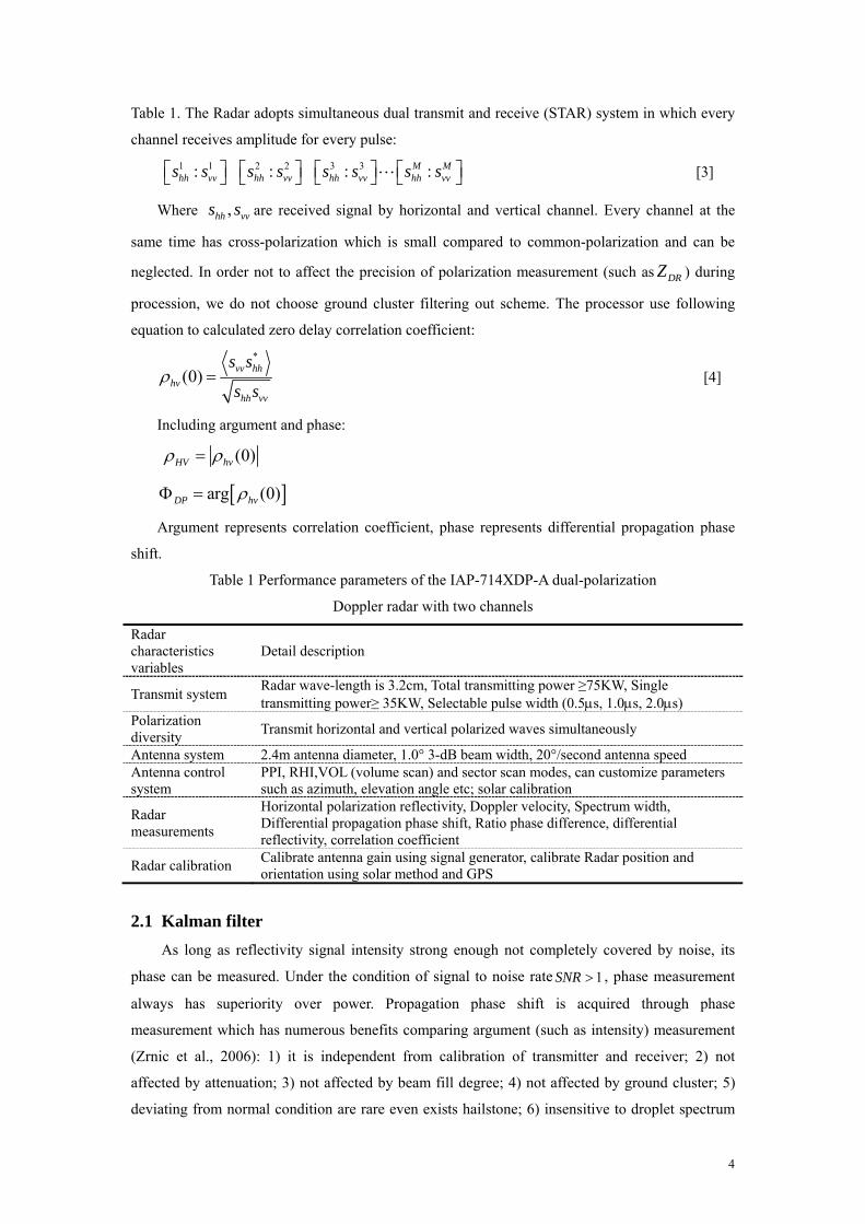
Table 1 Performance parameters of the IAP-714XDP-A dual-polarization

Doppler radar with two channels

Radar characteristics variables

Detail description

Transmit system Radar wave-length is 3.2cm, Total transmitting power ≥75KW, Single transmitting power≥ 35KW, Selectable pulse width (0.5s, 1.0s, 2.0s)

Polarization diversity

Transmit horizontal and vertical polarized waves simultaneously

Antenna system 2.4m antenna diameter, 1.0° 3-dB beam width, 20°/second antenna speed Antenna control system

PPI, RHI,VOL (volume scan) and sector scan modes, can customize parameters such as azimuth, elevation angle etc; solar calibration

Radar measurements

Horizontal polarization reflectivity, Doppler velocity, Spectrum width, Differential propagation phase shift, Ratio phase difference, differential reflectivity, correlation coefficient

Radar calibration Calibrate antenna gain using signal generator, calibrate Radar position and orientation using solar method and GPS

2.1 Kalman filter

As long as reflectivity signal intensity strong enough not completely covered by noise, its

phase can be measured. Under the condition of signal to noise rate 1SNR , phase measurement

always has superiority over power. Propagation phase shift is acquired through phase

measurement which has numerous benefits comparing argument (such as intensity) measurement

(Zrnic et al., 2006): 1) it is independent from calibration of transmitter and receiver; 2) not

affected by attenuation; 3) not affected by beam fill degree; 4) not affected by ground cluster; 5)

deviating from normal condition are rare even exists hailstone; 6) insensitive to droplet spectrum

5

variation; 7) it is easy to distinguish anomaly propagation.

Due to differential propagation phase shift Φ has obvious fluctuations and belong to high

frequency noise as for frequency domain. Thus many researchers (such as Hubbert et al., 1995)

designed low-pass filter to remove the high frequency noises to keep the average trend of curve.

But a specific filter relies on sample distance and the required smoothness (Hubbert et al.,,

1995).The paper utilize Kalman filter (Kalman, 1960) process Radar detected variable Φ to

acquire differential propagation phase shift Φ needed by attenuation correction. Kalman filter

uses mean square error as the optimal estimation criterion, seeks a set of recursive algorithm. It

adopts space model of signal and noise state, using estimated value of previous time and observed

value of current time to updates state variable, obtains current time estimation. In Kalman filter,

visual physical meaning of time region language is adopted, that is only observational data during

a limited time span are needed, thus relatively simple recursive algorithm can be applied and can

be extended to unsteady random processes, and the data storage is small. Therefore, Kalman is

suitable for computer real-time processing and calculating, it is an “Optimal Recursive Data

Processing Algorithm”.

When Radar remote sensing atmosphere, the to be measured state variable in every effective

irradiation volume affected not only by atmosphere turbulence and other possible noises, but also

by observational machine self noises. This can be abstracted to state variable estimation in discrete

time process which can be described as the following discrete random differential equation

1 1 1( ),k k k kx Ax B u w [5]

Define observation variable as z , the observation equation can be written as:

k k kz Cx v d [6]

Table 2 shows meaning of each term in the model. 1kw is random disturbance signals from

atmosphere state (process noise), kv is instrument noise (measurement noise), here assume they

are independent from each other and the distributions are known.

Table 2 Meaning of each term of discrete difference equation

Symbols Meaning

kx System state

A System matrix

, kB u State control variables

kz Measured value

C Observational matrix

kw Procession noise ),0(~)( QNwp

kv Measured noise ),0(~)( RNvp

Assume under ideal condition, there is a precipitation cell on Radar ray, its corresponding

6

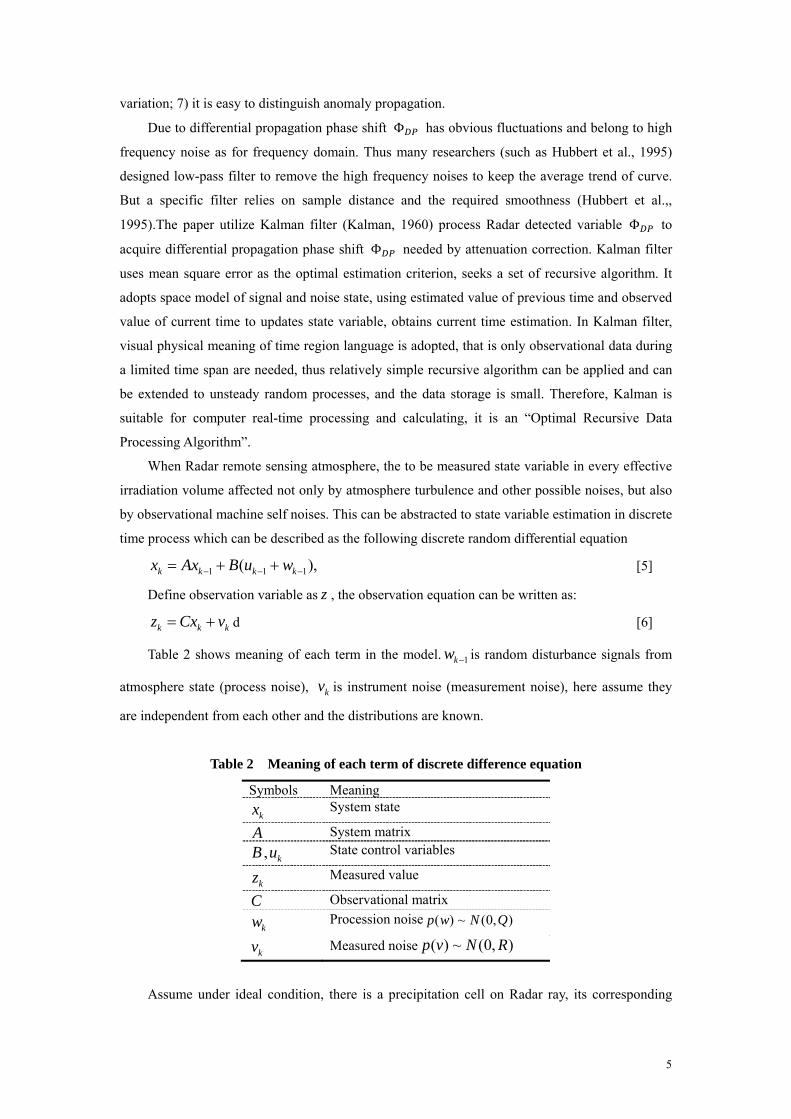
relationship with Φ is showed in Fig 1a. Ray enter precipitation cell from 0r , Φ increases.

When the ray reaches cell center, Φ change rate is greatest. Then ray passes cell center, Φ

increase rate slows down. After ray passes cell and enters non-precipitation area, Φ stop

increasing. If precipitation cell is homogenous, the differential propagation phase shift is indicated

in Fig 1b, that is in the whole homogenous precipitation cell from 0r to mr , Φ increases with a

constant rate, its slope indicates cell intensity, the more intense the precipitation cell, the greater

the Φ slope.

Fig.1 Relationship between ideal precipitation cell and differential propagation phase shift DP

( A. inhomogeneous precipitation cell, B. homogeneous precipitation cell)

During the procession, assume Radar ray propagation as the movement of moving object, the

mathematic model for its kinematic equations can be described by following differential equation,

thus describe the low of motion for differential propagation phase shift Φ :

212(r 1) r (r) (r)

(r 1) (r) (r)DP DP DP

DP DP

a r

ra

[7]

Where (r)DP and (r)DP are “location” and “velocity” of distance r respectively,

here refer to accumulated and unit ( DPK ) differential propagation phase shift respectively. Due to

short average distance resulted from Radar adjacent distance base processing, further process must

be do to use (r)DP in Eq. [7]; (r)a represents acceleration caused by uncertain factors such

as meteorological object, ambient, Radar detecting system etc from r to 1r , it reflects

undetectable caused by weather system itself and Radar detection system. (r)a can be assumed to

be a steady random sequence normally distributed which average value is zero and square error is

Q , besides ( )a k and ( )( )a l l k are not related to each other, that is the expectation for

(r)a is (r) 0E a , )1()}()({ kQlakaE K , where K is Kronecker function whose

characteristics are

0,0

0,1)(

k

kkK .

According to above discussion, Eqs. [5] and [6] change to:

r

ΦD

P

r0 rm

降水单体A

r

ΦD

P

r0 rm

降水单体

Bprecip. cell precip. cell

7

(r) (r 1) (r 1)X AX Ba [8]

(r) (r) (r)Z CX V [9]

Where, (r)

(r)(r)

DP

DP

X

, is state variable for observed weather system;

1

0

rA

r

, is

state transferring matrix for observed weather system;

2

2

rB

r

, is process noise, refer to the

corresponding weather system change noises when beam transfers from one irradiation volume to

another during Radar detection; 1 0C , is system observation matrix, Since differential

propagation phase shift is directly observed, the first element in C matrix is equal to 1, (r)a is

Gaussian white noise sequence called dynamic white noise vector whose average value is zero and

square error; (r)V Gaussian white noise sequence called observational white noise vector whose

average value is zero and square error, and does not correlated with (r)a ; Known system state and

observation equations, calculation can be accomplished through calculating prior state estimation

value and prior error covariance matrix, modifying matrix, updating observation value, updating

error covariance matrix etc (Zhang et al, 2001).

2.2 Filtration initialization

When using Kalman filtration algorithm, filtration initialization estimation value and error

covariance matrix are needed to be assigned. Fig 3 shows that there are areas with great

differential reflectivity fluctuation around Radar station during real Radar detection, which may

induced by processing method of Radar signal processing system, machine interior noises and

ground object noises etc. The fluctuation is varied up and down centered at a constant value.

Bringi et al. (2002) indicates that Radar recorded differential phase shift is the result of Radar

system and meteorological object, that is:

systemDPDP

rvsw

rhsw

tvsw

thsw

vhj

comeasco dffe rh

)(

)]()[(

arg)arg()arg(

)()()()(

)(2

[10]

Where Φ is meteorological object differential phase detected by Radar; ( )DP system is the

system differential phase shift which is a system error determined by the steady of system receiver

and transmitter. Comparisons of different time data show that differential phase shift of Radar zero

distance always drift to some extent which is not a constant value. This is related with Radar

stability, system stability and fixed phase difference may be change with time and are controlled

by temperature and humidity etc (Bringi et al., 2002). Therefore the first step in calculation is to

determine initial phase that is system phase difference for every scan line. Known from above

discussion, generally Φ fluctuation increases with decreases of signal to noise rate. Since all of

8

them are unbiased estimation, the points have obvious fluctuation can be substituted by the

average value of preceding several bases of every radial data. The paper uses 10 preceding points,

that is, if Radar observed with 150m base, then the corresponding average value is at distance of

1.5km. The initial condition need to be appointed when using Kalman filter algorithm. To assign

initial condition quickly during every scan line’s processing, the paper uses the detected value of

two initial bases after moving average to establish initial estimation, that is:

TrZZZX ]/))1()2(()2([)2|2(ˆ [11]

Initial estimation error is:

r

VV

r

V

rZZ

Z

XXX

DPDPDP

DP

DP

)1()2()1()2()2(

)2(

/))1()2((

)2(

)2(

)2(

)2|2(ˆ)2()2|2(~

[12]

From state Eq. [13]:

(2) (1)(1) (1) / 2DP DP

DP rar

[13]

And

(2) (1)(2) (1) (1) (1) (1) / 2 (1) / 2DP DP

DP DP DPra ra rar

[14]

Thus Eq. [8] can be written as:

r

VVraV

X )2()1(

2

)1()2(

)2|2(~

[15]

Covariance matrix for error estimation is:

rQrRrQ

rQQXXEP T

/24//

/)2|2(

~)2|2(

~)2|2(

2222

22

[16]

2.3 Comparison between Kalman and other filter

To verify merits of Kalman filter, assume Radar detection distance is 150km, base length is

150m. There are weather signals as showed in Fig.2a within detection distance. Various noises

induced the fluctuations of Radar echo signal, assume the noises are Gaussian white noise. Add

Gaussian white noise to original signal with signal to noise rate 10, the result after adding noise

showed in Fig.2b. Then use median and Kalman filter to filter contaminated signal, the results

showed in Fig.2c and 2d. The figures show that median and Kalman filter have similar filter effect,

they both keep the main characteristics of original signal. For median filter, the key problem is the

width of the filter window, different widths give different results in experiment, see Fig. 2c. The

two curves indicate results from two filter widths respectively. This shows that for different

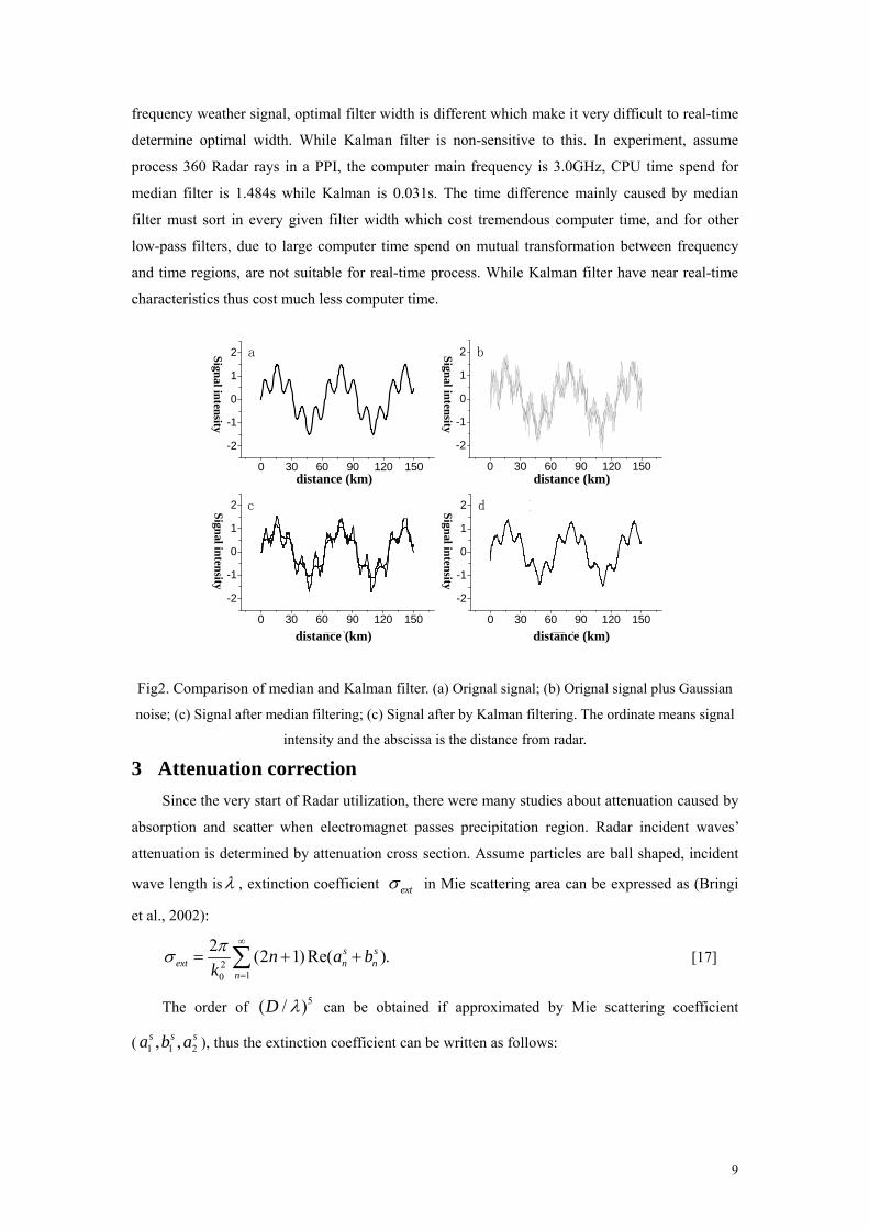
9

frequency weather signal, optimal filter width is different which make it very difficult to real-time

determine optimal width. While Kalman filter is non-sensitive to this. In experiment, assume

process 360 Radar rays in a PPI, the computer main frequency is 3.0GHz, CPU time spend for

median filter is 1.484s while Kalman is 0.031s. The time difference mainly caused by median

filter must sort in every given filter width which cost tremendous computer time, and for other

low-pass filters, due to large computer time spend on mutual transformation between frequency

and time regions, are not suitable for real-time process. While Kalman filter have near real-time

characteristics thus cost much less computer time.

Fig2. Comparison of median and Kalman filter. (a) Orignal signal; (b) Orignal signal plus Gaussian

noise; (c) Signal after median filtering; (c) Signal after by Kalman filtering. The ordinate means signal

intensity and the abscissa is the distance from radar.

3 Attenuation correction

Since the very start of Radar utilization, there were many studies about attenuation caused by

absorption and scatter when electromagnet passes precipitation region. Radar incident waves’

attenuation is determined by attenuation cross section. Assume particles are ball shaped, incident

wave length is , extinction coefficient ext in Mie scattering area can be expressed as (Bringi

et al., 2002):

210

2(2 1) Re( ).s s

ext n nn

n a bk

[17]

The order of 5( / )D can be obtained if approximated by Mie scattering coefficient

( 1 1 2, ,s s sa b a ), thus the extinction coefficient can be written as follows:

0 30 60 90 120 150

-2

-1

0

1

2

信号

强度

距离

原始信号a

0 30 60 90 120 150

-2

-1

0

1

2

信号强度

距离

信号加高斯噪声b

0 30 60 90 120 150

-2

-1

0

1

2

信号

强度

距离

中值滤波后信号c

0 30 60 90 120 150

-2

-1

0

1

2

信号强

度

距离

kalman滤波后信号d

distance (km) distance (km)

distance (km) distance (km) S

ignal in

tensity

Sign

al inten

sity

Sign

al inten

sity S

ignal in

tensity

10

1 1 220

23

23Re( ) 5Re( )

16 5( ) 16 2 3

s s sext

r

r

a b ak

DD i t u w

[18]

Where, r is complex relative dielectric constant, definitions for , ,t u w please refer to

Hulst et al. (1981). Here Re represents real part of complex, 1i , D is diameter of particle.

Bringi et al (2001) showed that following exponent relation can be used as first-order

approximation for extinction coefficient:

next C D [19]

To use differential propagation phase shift do attenuation correction, the relation between unit

differential propagation phase shift and attenuation rate must be solved first. According to Eq. [19],

for 3cm wave length Radar, the particle’s diameter is mmD 81.0 . If use first-order

approximation, 9.3n , for particle’s diameter mmD 105 , the corresponding 6.4n . To

simplify discussion, the relation between attenuation and differential propagation phase shift is

inducted, here 4n . Thus attenuation rate can be expressed as:

3 1

3 4

4.343 10 ( ) ( ) ;

4.343 10 ( ) .

h ext D N D dD dB km

C D N D dD

[20]

If use drop size distribution term to express DPK , then:

1180Re[ ( ) ( )] ( ) (deg )DP h vK f D f D N D dD km

[21]

Here hf and vf are channel forward scattering phase for horizontal and vertical polarization.

Therefore attenuation correction based on unit differential propagation phase shift DPK is (Park

et al., 2005):

h h DPc K [22]

Here ha is attenuation rate which expresses effects from various factors affecting DPK

(Gorgucci et al., 2005). And the accumulative differential propagation phase shift Φ is the

accumulative variable of double DPK . Then accumulative attenuation is:

2

12 1

2 1

( ) ( ) 2 ( )

[ ( ) ( )].

r

H H h DPr

h DP DP

A r A r c K r dr

c r r

[23]

Here 1 2,r r are two distances on Radar ray. If assign zero to 1r , that is the first base for Radar,

then the above equation changes to:

)]0()([)( DPDPhH rCrA [24]

11

Where, 0)( 1 rAH , (0)DP is differential propagation phase shift for the first base of

Radar ray, that is ( )DP system in Eq. [10], which represents system initial differential propagation

phase shift. Then the attenuation correction for Radar reflectivity can be expressed as (Park et al.,

2005):

)]0()([)()()()( DPDPhmHm rcrZrArZrZ [25]

Here ( )mZ r is Radar detection value at distance r ; ( )HA r is correction at distance r use

differential propagation phase shift; ( )Z r is the result after correction. It can be seen that they

are linearly related when using differential propagation phase shift to correct reflectivity.

4 Case analysis

On May 15, 2007, a low trough controlled the east of China; the northeastern China locates in

front of 500hPa trough. On 850hPa level, the trough stretches southward from the northeastern

China till South of Yangtze River Basin at 08 o’clock (Beijing Time, same as below). At 14

o’clock, there a low vortex was generated above Jilin area which maintained at Jilin Province in

the northeastern China till 20 o’clock. It can be seen that the low vortex cloud system developed

and moved eastward from the May 15 satellite cloud map. The sounding profile at Changchun

station shows that the difference between dew point and temperature is big with unsaturated lower

atmosphere at 8 o’clock May 15. At 20 o’clock, the lower atmosphere became saturated. Around

21 O’clock May 15, there was precipitation in Yitong area, Jilin Province.

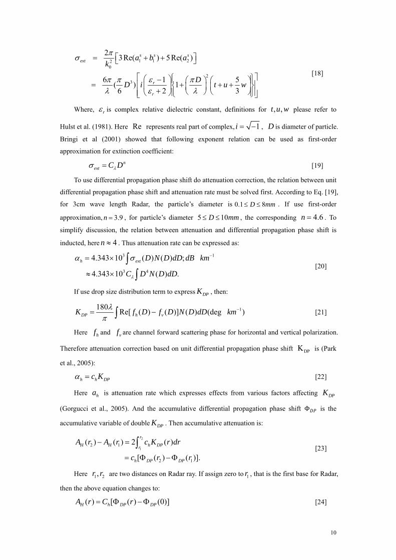
4.1 Case filtration

Fig.3 is the Radar ray with 195 azimuth and 1 elevation angle, the variance of Φ with

distance is showed by dash lines. Following processing is based on Radar polar coordinate system.

The figure shows that differential propagation phase shift departure from theoretical value

increases with distance accompanied by fluctuations. The fluctuations mainly induced by

atmosphere self fluctuation and Radar machine interior detection noise etc, that is processing and

measurement noises in Kalman filter. Fluctuations are obvious especially around Radar station and

far part of Radar ray. According to above discussions, the fluctuations are unbiased and have big

initial phase shit at the same time. In this case, the initial phase is 103°, and there appear

fluctuation signals with long nail shape on Radar ray, the signal is an obvious backward

propagation phase shift effect. Compared with reflectivity in Fig 5, we find that at 5km and

11km where effect appears, the reflectivity is greater than adjacent. Besides obvious effect,

there also exists unobvious backward propagation effect which structure showed in Fig 5 as minor

fluctuation, and high frequency noises from other noise source. The object of this paper using

Kalman filter is to solve the problems and obtain differential propagation phase shift curve used

by attenuation correction.

12

Fig.3 Differential propagation phase shift with distance before and after filtration. The ordinate means

differential propagation phase shift DP (/km) and the abscissa is the distance from radar.

During detection, Radar signal is contaminated by atmosphere unsteady noise and Radar

system interior machine noise. Using filtered Radar ray showed as real line in Fig. 3, it can be

seen that noise effect is reduced and the backward scattering effect of polarization Radar

observed Φ (abnormal echo in Fig 3) is also canceled

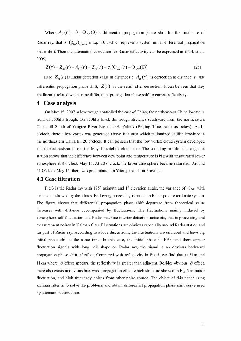
The differential propagation phase shifts of RHI data for the same time are processed use

Kalman filter, the results showed in Fig 4. The figure shows that differential propagation phase

shift Φ obviously improved after filtration. The figure has great fluctuations before filtration

which directly affect the stability and correct of afterward attenuation correction, while after

filtration, the figure is more smooth basically filter out effect and random noises.

Fig.4 Comparison of differential propagation phase shift DP (/km) before and after filtration, The

ordinate means height H (km) and the abscissa is the distance R (km) from radar.

4.2 Attenuation correction for a case

0 10 20 30 40 50 60 70 80

100

110

120

130

140

150

160

170

距离R(km)

差分

传播

相移

D

P(0 /k

m)

before filterafter filter

异常回波

区域I

区域II

distance (km)

Region I

Region II Abnormal echo

D

P ( /km

)

H (k

m)

distance (km)

13

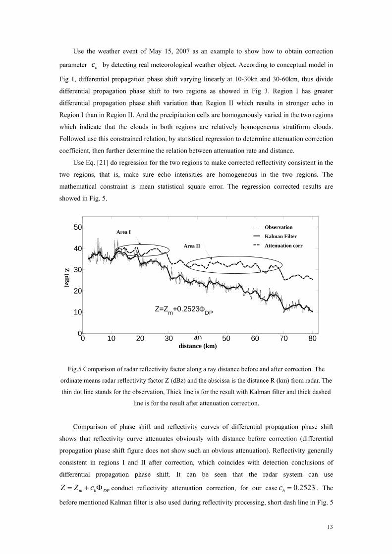
Use the weather event of May 15, 2007 as an example to show how to obtain correction

parameter nc by detecting real meteorological weather object. According to conceptual model in

Fig 1, differential propagation phase shift varying linearly at 10-30kn and 30-60km, thus divide

differential propagation phase shift to two regions as showed in Fig 3. Region I has greater

differential propagation phase shift variation than Region II which results in stronger echo in

Region I than in Region II. And the precipitation cells are homogenously varied in the two regions

which indicate that the clouds in both regions are relatively homogeneous stratiform clouds.

Followed use this constrained relation, by statistical regression to determine attenuation correction

coefficient, then further determine the relation between attenuation rate and distance.

Use Eq. [21] do regression for the two regions to make corrected reflectivity consistent in the

two regions, that is, make sure echo intensities are homogeneous in the two regions. The

mathematical constraint is mean statistical square error. The regression corrected results are

showed in Fig. 5.

Fig.5 Comparison of radar reflectivity factor along a ray distance before and after correction. The

ordinate means radar reflectivity factor Z (dBz) and the abscissa is the distance R (km) from radar. The

thin dot line stands for the observation, Thick line is for the result with Kalman filter and thick dashed

line is for the result after attenuation correction.

Comparison of phase shift and reflectivity curves of differential propagation phase shift

shows that reflectivity curve attenuates obviously with distance before correction (differential

propagation phase shift figure does not show such an obvious attenuation). Reflectivity generally

consistent in regions I and II after correction, which coincides with detection conclusions of

differential propagation phase shift. It can be seen that the radar system can use

DPhm cZZ conduct reflectivity attenuation correction, for our case 2523.0hc . The

before mentioned Kalman filter is also used during reflectivity processing, short dash line in Fig. 5

0 10 20 30 40 50 60 70 800

10

20

30

40

50

斜距R/km

反射

率Z

/dB

Z

实测值

滤波结果衰减订正结果

Z=Zm

+0.2523DP

区域I

区域IIArea II

Area I Observation

Kalman Filter

Attenuation corr

distance (km)

Z (d

Bz)

14

represents observed value and solid line is results after filtration. Here filter reflectivity to a certain

degree is good for understanding its main meteorological information. The method utilizing real

echo to determine correction coefficient has great practical value and always more effective.

To verify above results in our radar system, apply the correction relation to correct radar

detected RHI data, the results are showed in Fig. 6.

Fig.6 Comparison of radar reflectivity before and after correction. The ordinate means height H

(km) and the abscissa is the distance R (km) from radar.

In general, during the process, zero-layer bright band has earthward trend with distance

before correction, while basically keep horizontal after correction. It is a stratiform cloud

precipitating, the atmosphere is stable and horizontally homogeneous. Thus the trend before

correction is incorrect and coincides with weather situation after correction.

Comparison between before and after correction figures show that the correction method has

numerous merits: The two figures hardly have differences before and after correction for A region

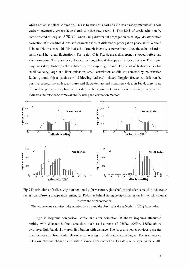
in due to light attenuation since Radar ray does not pass strong precipitation area. Do statistical to

reflectivity of each point with a constant interval Z before and after correction for A region,

the number distribution showed in Fig.8a and 8b. The figure shows that number distribution

pattern keep unchanged before and after attenuation correction with average values 40.438dBz

and 40.698dBz respectively which has little difference. Thus the basic characteristics keep

unchanged in weak precipitation area after attenuation correction this way.

Radar ray appear obvious attenuation in B and further regions after passed strong

precipitation region between regions A and B in Fig. 6. Following above statistical method, results

for the B and further regions are showed in Fig.7c and 7d. The figures show that the average value

is 27.184dBz and 37.321dBz which indicate serious attenuation for the entire B and further

regions. At the same time, the reflectivity number distribution spectrum width narrowed after

correction, while spectrum distribution pattern, such as distribution of peak numbers, basically

keep unchanged. Such change of spectrum pattern further illustrates that the stability of the

correction method. In Fig.7d, there appears many small echoes after correction between 5-25dBz

H (k

m)

distance (km)

15

which not exist before correction. This is because this part of echo has already attenuated. These

entirely attenuated echoes have signal to noise rate nearly 1. This kind of weak echo can be

reconstructed as long as 1SNR when using differential propagation shift Φ do attenuation

correction. It is credible due to self characteristics of differential propagation phase shift. While it

is incredible to correct this kind of echo through intensity superposition, since the echo is hard to

restore and has great fluctuations. For region C in Fig. 6, great discrepancy showed before and

after correction. There is echo before correction, while it disappeared after correction. The region

may caused by tri-body echo induced by zero-layer light band. This kind of tri-body echo has

small velocity, large and litter pulsation, small correlation coefficient detected by polarization

Radar, ground object (such as wind blowing leaf etc) induced Doppler frequency shift can be

positive or negative with great noise and fluctuated around minimum value. In Fig.4, there is no

differential propagation phase shift value in the region but has echo on intensity image which

indicates the false echo removal ability using the correction method.

Fig.7 Distributions of reflectivity number density for various regions before and after correction. a,b. Radar

ray in front of strong precipitation region, c,d. Radar ray behind strong precipitation region, left to right column:

before and after correction.

The ordinate means reflectivity number density and the abscissa is the reflectivity (dBz) from radar.

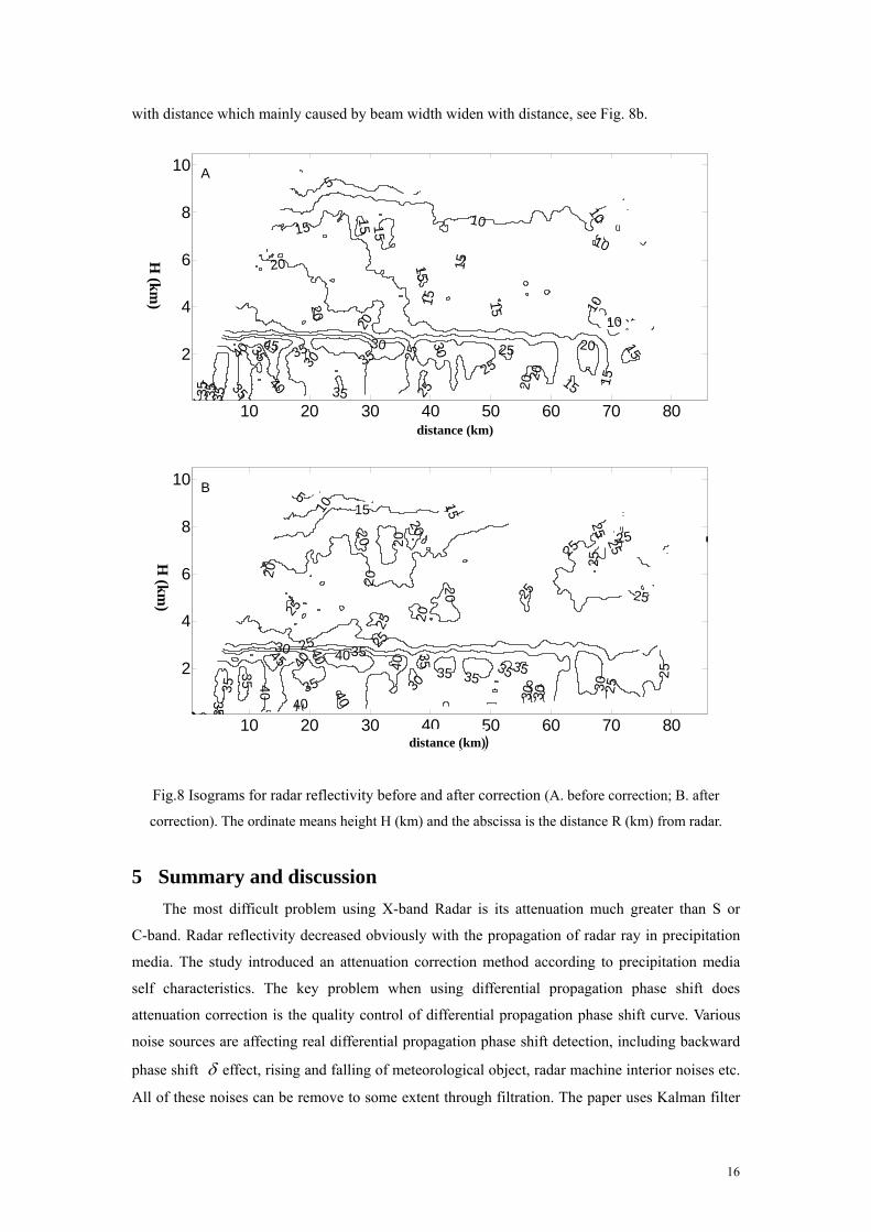
Fig.8 is isograms comparison before and after correction. It shows isograms attenuated

rapidly with distance before correction, such as isograms of 25dBz, 20dBz, 15dBz above

zero-layer light band, show arch distribution with distance. The isograms nearer obviously greater

than the ones far from Radar Below zero-layer light band as showed in Fig.8a. The isograms do

not show obvious change trend with distance after correction. Besides, zero-layer wider a little

5 10 15 20 25 30 35 40 45 50 550

500

1000

1500

平均值:37.3207

反射率

数密

度

d

5 10 15 20 25 30 35 40 45 50 550

500

1000

1500

平均值:27.184

反射率

数密

度

c

25 30 35 40 45 50 550

100

200

300

400

平均值:40.6983

反射率

数密

度

b

25 30 35 40 45 50 550

100

200

300

400

平均值:40.4376

反射率

数密

度

a

reflectivity (dBz) reflectivity (dBz)

reflectivity (dBz) reflectivity (dBz)

Mean: 27.184 Mean: 37.321

Mean: 40.698 Mean: 40.438

Nu

mb

er den

sity

Nu

mb

er den

sity

Nu

mb

er den

sity

Nu

mb

er den

sity

16

with distance which mainly caused by beam width widen with distance, see Fig. 8b.

Fig.8 Isograms for radar reflectivity before and after correction (A. before correction; B. after

correction). The ordinate means height H (km) and the abscissa is the distance R (km) from radar.

5 Summary and discussion

The most difficult problem using X-band Radar is its attenuation much greater than S or

C-band. Radar reflectivity decreased obviously with the propagation of radar ray in precipitation

media. The study introduced an attenuation correction method according to precipitation media

self characteristics. The key problem when using differential propagation phase shift does

attenuation correction is the quality control of differential propagation phase shift curve. Various

noise sources are affecting real differential propagation phase shift detection, including backward

phase shift effect, rising and falling of meteorological object, radar machine interior noises etc.

All of these noises can be remove to some extent through filtration. The paper uses Kalman filter

10 20 30 40 50 60 70 80

2

4

6

8

10

距离R(km)

高度

H(k

m)

5

10

10

10

10

10

15

15

15

15

15 15

15

15

15

1520

20

20

20

20

20

25 25

25

25

30

30

30

3535

35

35

35

35

35

35

40

40

45

A

10 20 30 40 50 60 70 80

2

4

6

8

105

10 15

15

20

20

20

20

20

2020

25

25

25

25

25

25 25

25

25

25

25

25

2530

30 30

3030

35

35

35

35

35353535

35

3540

40

40

40 40

40

40

45

距离R(km)

高度

H(k

m)

B

H (k

m)

H (k

m)

distance (km)

distance (km)

17

to deal with differential propagation phase shift DP of dual-polarization radar. This method is

an optimal self regression data process algorithm which makes it an optimal and most efficient for

all problems solving. Each term has definite physical meaning and has great practical value.

According to attenuation correction method, if we do not remove noises in Radar received

differential propagation phase shift before correction, there is high possibility that backward

propagation phase shift effect and other noises may much greater than differential propagation

phase shift itself which made serious distortion to corrected reflectivity then exert huge negative

effect on stability and accuracy of correction. The study according to the self characteristics of

differential propagation phase shift, utilizes the observed data by the X-band dual polarization

Doppler radar of Institute of Atmospheric Physics, Chinese Academy of Sciences, through stable

stratiform cloud case study, compares changes of RHI images and number density distribution

before and after correction, indicates good stability of filtered propagation phase shift to correction

of reflectivity factor. For weak echo situation, the stability of the correction method is like Radar

nearby area of stratiform cloud in the paper. Further investigation of many weak echo cases show

that the stability and accuracy of the correction method only depend on accuracy of differential

propagation phase shift not matter weak or strong echo. Under weak echo condition, though

backward propagation phase shift is small, other noises still exists and more serious, result in

necessary to filter differential propagation phase shift. It has certain practical value to determine

attenuation correction coefficient statistically by collecting numerous homogeneous statiform

cloud precipitation detection data of different time, same location, same Radar, on the basis of

filtration. Further studies are needed to establish robust attenuation correction coefficient suitable

for the Radar system by more observational data collection.

Acknowledgments

This work was supported by the National Natural Science Foundation of China (Grant No.

40875080) and Ministry of Science and Technology of China (Grant No. 2006BAC12B01-01).

18

References

Anagnostou, E.N., M.N. Anagnostou, W.F., Krajewski, A. Kruger, and B.J. Miriovsky, 2004.

High-Resolution Rainfall Estimation from X-Band Polarimetric Radar Measurements[J]. Journal

of Hydrometeorology, 5(1): 110-128.

Bringi, V.N., 2001. Correcting C-Band Radar Reflectivity and Differential Reflectivity Data for Rain

Attenuation: A Self-Consistent Method With Constraints[J]. IEEE Transcations Geoscience and

Remote Sensing, 39(9): 1906-1915.

Bringi, V.N. and V. Chandrasekar, 2002. Polarimetric Doppler Weather Radar: Principles and

Applications[M]. Cambridge University Press.

Gorgucci, E. and V. Chandrasekar, 2005. Evaluation of Attenuation Correction Methodology for

Dual-Polarization Radars: Application to X-Band Systems[J]. Journal of Atmospheric and

Oceanic Technology, 22(8): 1195-1206.

Gorgucci, E., G. Scarchilli , V. Chandrasekar , P.F. Meischner and M. Hagen, 1998. Intercomparison of

Techniques to Correct for Attenuation of C-Band Weather Radar Signals[J]. Journal of Applied

Meteorology, 37(8): 845-853.

H. C.van de Hulst, 1981. Light Scattering by Small Particles[M]. New York: Dover.

Hildebrand, P. H, 1978. Iterative Correction for Attenuation of 5 cm Radar in Rain[J]. Journal of

Applied Meteorology, 17(4): 508-514.

Hubbert, J. and V.N. Bringi, 1995. An Iterative Filtering Technique for the Analysis of Copolar

Differential Phase and Dual-Frequency Radar Measurements[J]. Journal of Atmospheric and

Oceanic Technology, 12(3): 643-648.

Johnson, B.C. and E.A. Brandes, 1987. Attenuation of a 5-cm Wavelength Radar Signal in the

Lahoma-Orienta Storms[J]. Journal of Atmospheric and Oceanic Technology, 4(3): 512-517.

Kalman, R.E, 1960. A new approach to linear filtering and prediction problems[J]. Transactions of the

ASME. Series D: Journal of Basic Engineering, 82:35-45.

Park, S.G., V.N. Bringi, V. Chandrasekar, M. Maki, and K. Iwanami, 2005. Correction of Radar

Reflectivity and Differential Reflectivity for Rain Attenuation at X Band. Part I: Theoretical and

Empirical Basis[J]. Journal of Atmospheric and Oceanic Technology, 22(11): 1621-1632.

Qin Y., B. Li and P. Zhang, 2006. A Study of the Relationship Between Radar Reflectivity of Rain and

Relative Humidity of Atmosphere[J](in Chinese).Chinese Journal of Atmospheric Sciences,

30(2):351-359.

Ryzhkov, A. and D. Zrni, 1996. Assessment of Rainfall Measurement That Uses Specific Differential

Phase[J]. Journal of Applied Meteorology, 35(11): 2080-2090.

Seliga, T.A. and V.N. Bringi, 1976. Potential Use of Radar Differential Reflectivity Measurements at

Orthogonal Polarizations for Measuring Precipitation[J]. Journal of Applied Meteorology, 15(1):

69-76.

Wiener, N, 1949. Extrapolation, Interpolation, and Smoothing of Stationary Time Series[J]. New York:

Wiley.

Zhang P., B. Du and T. Dai, 2001. Radar Meteorology[M](in Chinese), Beijing: China Meteorological

Press,511.

19

Zrnic, D.S., V.M. Melnikov, and J.K. Carter, 2006. Calibrating Differential Reflectivity on the

WSR-88D[J]. Journal of Atmospheric and Oceanic Technology, 23(7): 944-951.