Journal of Applied Mechanics and Technical Physics, Vol. 54, No. 4, pp. 900–912, 2013.

Original Russian Text c© S.L. Davis, T.B. Dittmann, G.B. Jacobs, W.S. Don.

DISPERSION OF A CLOUD OF PARTICLES BY A MOVING SHOCK:

EFFECTS OF THE SHAPE, ANGLE OF ROTATION, AND ASPECT RATIO

UDC 532; 533.7S. L. Davisa, T. B. Dittmanna, G. B. Jacobsa, and W. S. Donb

Abstract: This paper discusses the particle-laden flow development from a cloud of particles in

an accelerated flow behind a normal moving shock. The effects of the aspect ratio of a rectangular

and ellipsoidal cloud and the cloud’s angle of attack with respect to the carrier flow are stud-

ied. Computations are performed with an in-house high-order weighted essentially non-oscillatory

(WENO-Z) finite-difference scheme-based Eulerian–Lagrangian solver that solves the conservation

equations in the Eulerian frame, while particles are traced in the Lagrangian frame. Streamlined

elliptically shaped clouds exhibit a lower dispersion than blunt rectangular clouds. The averaged and

root-mean-square locations of the particle coordinates in the cloud show that the cloud’s stream-

wise convection velocity increases with decreasing aspect ratio. With increasing rotation angle, the

cross-stream dispersion increases if the aspect ratio is larger than unity. The particle-laden flow de-

velopment of an initially moderately rotated rectangle is qualitatively and quantitatively comparable

to the dispersion of an initially triangular cloud.

Keywords: dispersion of particles, shock wave, high-order finite-difference monotonic scheme.

DOI: 10.1134/S0021894413060059

INTRODUCTION

Particle-laden and droplet-laden flows play an important role in high-speed technologies, such as solid rocket

propulsion systems and high-speed liquid-fuel combustors. Shock waves occur in scramjet combustors and interact

with fuel particles in the resultant supersonic flow. Accurate tracing of fuel droplet trajectories would allow for more

precise ignition and combustion, boosting the overall engine efficiency. The physical complexity of simultaneously

resolving particle-turbulence, shock-turbulence, and shock-particle interactions along with the large range of spatial

and temporal scales pose high demands on both experimental and computational analysis. Experimental analysis is

limited to large-scale observation due to high velocities, while first principle computations are expensive and models

are not optimal.

Significant effort has been applied toward the improvement of empirical governing models for the particle

phase through the investigation of acceleration of an individual particle behind a shock wave. Boiko et al. [1]

determined the drag of a droplet behind a shock by comparing the known relaxation times of a hard sphere to their

experimentally measured droplet relaxation times. Sun et al. [2] numerically studied the dynamic drag coefficient

of a spherical particle behind a shock wave. A reflected bow shock was observed in front of the spherical particle,

and, as the shock wave traversed over the sphere, a Mach reflection formed. The Mach reflection proceeded to the

rear center of the sphere before converging with the Mach reflection from the other side. This caused shock focusing

to occur, and a region of very high pressure at the rear of the spherical particle was formed. This region of high

aSan Diego State University, San Diego, CA 92182; gjacobs@mail.sdsu.edu. bHong Kong Baptist University,Hong Kong, China; wsdon@math.hkbu.edu.hk. Translated from Prikladnaya Mekhanika i Tekhnicheskaya Fizika,Vol. 54, No. 6, pp. 45–59, November–December, 2013. Original article submitted July 9, 2012.

900 0021-8944/13/5406-0900 c© 2013 by Pleiades Publishing, Ltd.

pressure resulted in a brief negative drag. Their numerical data matched experimental data within 10%. Loth [3]

investigated the effect of compressibility and rarefaction on a spherical particle. Boiko et al. [4] also studied particles

of different shapes. Comparing a cubical and a spherical particle, they found that the drag was predominantly a

function of the frontal area of the particle. Therefore, the relative bluntness of the shapes did not significantly affect

the particle dynamics.

A limited number of studies were performed on the dynamics of a large number of particles in a high-speed

flow. Olim et al. [5] studied the attenuation of a normal shock wave in a homogeneous gas–particle mixture. Kiselev

et al. [6, 7] compared simulations based on Boiko’s empirical particle model to shock-tube experiments on the

dispersion of a cloud of plexiglas and bronze particles in the accelerated flow behind a moving shock [6, 7]. Not

only did they visualize the particle dynamics and dispersion, they also matched some of their results quantitatively

to the experimental dispersions. Jacobs et al. [8, 9] developed a high-order/high-resolution Eulerian–Lagrangian

scheme based on the same empirical physical governing model as that proposed by Kiselev et al. [6]. Extensive

high-order/high-resolution results showed good comparisons with experimental results, while small-scale turbulent

structures were resolved with improved efficiency. In [8], we studied the effect of the initial shape of the cloud

geometry on the dispersion of particles. It was shown that the aerodynamics of the shape significantly altered the

cross-stream dispersion of particles.

This paper extends the investigation of the cloud geometry effect on the dispersion of particles in an accel-

erated flow behind a moving shock. We study the effect of the aspect ratio and rotation of the cloud and present

detailed statistics of the particle dispersion in terms of the averaged particle coordinates. This investigation is

part of our ongoing effort to thoroughly validate Eulerian–Lagrangian methods against shock-tube experiments for

shocked particle-laden flow.

1. PHYSICAL MODEL AND GOVERNING EQUATIONS

In the particle-source-in-cell (PSIC) method, the Eulerian continuum equations are solved for the carrier

flow in the Eulerian frame, while particles are traced along in the Lagrangian frame. In the following, we present

the coupled system of Euler equations that govern the gas flow and kinematic equations that govern the particle

motion. We shall assign the subscript p for the particle variables and f for the gas variables at the particle position.

Variables without the subscript refer to the gas variables unless specified otherwise. For a more detailed discussion

of the physical model and governing equations, the readers are referred to [8].

1.1. Euler Equation in the Eulerian Frame

The governing equations for the carrier flow are the two-dimensional Euler equations in Cartesian coordinates

given by

Qt + Fx +Gy = S, (1)

where

Q = (ρ, ρu, ρv, E)T, F = (ρu, ρu2 + P, ρuv, (E + P )u)T,

G = (ρv, ρuv, ρv2 + P, (E + P )v)T, P = (γ − 1)(E − ρ(u2 + v2)/2), γ = 1.4.

The system of equations is closed by the equation of state

T = γPM2/ρ,

where M = U/√γRT is a reference Mach number and U and T are the reference velocity and reference temperature,

respectively. The source term S accounts for the effect of the particles on the carrier gas.

1.2. Particle Equation in the Lagrangian Frame

Particles are tracked individually in the Lagrangian frame. The kinematic equation describing the particle

position �xp is

901

dxp

dt= vp,

where xp is the particle radius-vector and vp is the particle velocity vector.

The particles’ acceleration is governed by Newton’s second law forced by the drag on the particle. With

particles assumed spherical, we take the drag as a combination of the Stokes drag corrected for high Reynolds and

Mach numbers and the pressure drag, leading to the following equations governing the particle velocity:

dvp

dt= f1

vf − vp

τp− 1

ρp∇P

∣∣∣f

(2)

(vf is the velocity of the gas at the particle position and ρp is the particle density).

The first term on the right-hand side of Eq. (2) describes the particle acceleration resulting from the velocity

difference between the particle and the gas; the second term in the right-hand side of this equation represents the

particle acceleration induced by the pressure gradient in the carrier flow at the particle position. The particle time

constant τp = Re d2pρp/18 is a measure for the reaction time of the particle to the changes in the carrier gas, where

dp is the particle diameter, Re = UL/ν is the Reynolds number of the carrier gas flow, L is the reference length,

and ν is the dynamic viscosity.

In this study, we assume that the Reynolds number is high, and we, therefore, do not model viscous effects

in the governing Eulerian equations for the gas flow (1).

The empirical correction factor

f1 =3

4

(

24 + 0.38Ref +4√

Ref

)(

1 + exp(

− 0.43

M4.67f

))

ensures an accurate determination of the acceleration within 10% of the measured particle acceleration for Reynolds

numbers up to Ref = |vf − vp|dp/ν ≈ 104 and Mach numbers up to Mf = |vf − vp|/√Tf = 1.2.

From the first law of thermodynamics and Fourier’s law for heat transfer, we obtain the equation for tem-

perature

dTp

dt=

1

3

Nu

Pr

Tf − Tp

τp,

where Pr = 1.4 is the Prandtl number, taken as its typical value for air in this paper, and Nu = 2+√

Ref Pr0.33 is

the Nusselt number corrected for high Reynolds numbers.

1.3. Source Term S for the Euler Equation

Each particle generates a momentum and energy that affect the carrier flow. The volume-averaged summa-

tion of all these contributions gives a continuum source contribution to the momentum and energy equation (1):

Sm(x) =

Np∑

i=1

K(xp,x)Wm, Se(x) =

Np∑

i=1

K(xp,x)(Wm · vp +We).

Here K(x, y) = K(|x − y|)/V is a normalized weight function that distributes the influence of each particle onto

the carrier flow, Wm = mpf1(vf − vp)/τp and We = mp(Nu /(3Pr ))(T −Tp)/τp are weight functions describing the

momentum and energy contributions of one particle, respectively, mp is the mass of one spherical particle, which

can be derived from τp, and Np is the total number of particles in a finite volume V .

1.4. Flow and Particle Solver

The governing equations are discretized and solved using the weighted essentially non-oscillatory WENO-Z-

based PSIC scheme proposed by Jacobs et al. [8, 9].

The nonlinear nature of the hyperbolic Euler equations admits finite-time singularities in the solution even

when the initial condition is smooth. It is important that the numerical methods employed avoid non-physical

oscillations, also known as the Gibbs phenomenon, when the solution becomes discontinuous.

Among many high-order shock-capturing schemes, the classical WENO conservative finite-difference schemes

for conservation laws by Shu et al. [10] have been very successfully employed for the simulation of fine-scale and

delicate structures of the physical phenomena related to shock-turbulence interactions [11–14].

902

The improved version of the classical WENO conservative finite-difference scheme, namely, WENO-Z

scheme [15, 16] is ideally suited for computing a shock wave interacting with a cloud of particles due to the

complicated shock structures of the problem and the importance of preserving high-order resolution to resolve the

small-scale interactions present in a particle-laden shocked flow.

The essence of the WENO scheme is the use of adaptive stencils. The method creates a stencil over the

computational domain, in which a smoothness indicator is employed to estimate within which substencils the shocks

lie. The method then assigns an essentially zero weight to low-order local interpolation polynomials of the flux,

based on the values from substencils that contain high gradients and/or shocks to prevent Gibbs oscillations.

In computational cells where no shock is present, a high-order upwinded central finite-difference scheme is

used to calculate the flow properties. In shocked regions, however, a centered interpolation will produce undesirable

Gibbs oscillations. With an ENO interpolation, these oscillations are essentially removed. The ENO interpolation

is only necessary in WENO-domains identified by the smoothness indicator. The WENO scheme ensures that

the formal order of accuracy/resolution in smooth regions of the simulation remains intact as best as one can do.

The flow solver calculates the parameters of the flow by solving the Euler equations with a particle source term

weighted onto the flow at grid points within the domain. The particle variables are then calculated by using a high-

order ENO interpolation with a spline function of the same order of accuracy as the flow solver to avoid excessive

computational errors.

2. RESULTS AND DISCUSSION

We perform simulations based on the fifth-order WENO-Z-based PSIC algorithm for flow evolution when

a shock runs through a cloud of particles. To summarize the algorithm, we approximate the system of hyperbolic

Euler equations (1) in the Eulerian frame at each grid point:

dQ

dt= −∇ · F (Q) + S(xp − x). (3)

The particles are individually traced in the Lagrangian frame:

dxp

dt= vp,

dvp

dt= f1

vf − vp

τp− 1

ρp∇P

∣∣∣f;

dTp

dt=

1

3

Nu

Pr

Tf − Tp

τp, p = 1, . . . , Np. (4)

Interpolation determines vf and Tf , while weighting determines S(xp − x).

We employ the third-order Total Variation Diminishing Runge–Kutta (RK-TVD) scheme

U1 = Un +Δt L(Un), U2 =3Un +U1 +Δt L(U1)

4, Un+1 =

Un + 2U2 + 2Δt L(U2)

3,

where L is the spatial operator as in the right side of Eqs. (3) and (4). The Courant–Friedrichs–Lewy (CFL) number

is set to 0.4.

We initialize a right-running Mach-three (Ms = 3) shock at xs = 0.175 in a rectangular domain [0; 3] ×[−0.611; 0.611]. Inflow and outflow boundary conditions are specified in the x direction, and periodic boundary

conditions are imposed in the y direction. A uniformly distributed cloud of bronze particles is seeded in a rectangular

domain [0.175; 0.352]× [−0.044; 0.044], with a zero initial velocity. The volume concentration of the particles in

the cloud is 4%. The particle response time and density are τp = 51.69 and ρp = 7.42 · 104, respectively. We take

the Reynolds number needed to compute the particle traces according to the experiment at Ref = 3.387 · 107. In

the following computations, the number of grid points used to solve the Euler equation in the Eulerian frame is

1500× 1500 in the x and y directions, respectively. Clouds consisting of 3.9 · 109 real particles were approximated

using 40 000±100 computational particles depending upon the cloud shape. The dimensions of different clouds were

determined based on the shape and aspect ratio desired, and particles were seeded accordingly to provide for an

even distribution. As an example, the square cloud (shape) shown in Fig. 1 was arranged with 200× 200 particles.

We briefly summarize the effect of the initial cloud shape that was studied in [8] to set the stage for the

analysis of the effect of the aspect ratio and rotation of the cloud. In [8], we compared rectangular, circular, and

903

NSW

Up, Tp, dp

Nx

NyU, Tx

y

Fig. 1. Initial state of the particle-laden flow (NSW is the normal shock wave).

(a) (b) (c)

Fig. 2. Vorticity contours in an accelerated gas flow behind a moving shock at t = 0.1 for cloudsof different shapes: (a) circular cloud; (b) rectangular cloud; (c) triangular cloud.

triangular clouds with the same particle volume concentrations. The clouds cover the same geometric area and are

initialized so that the cloud’s location is directly adjacent to the downstream side of the normal shock wave.

At early times, the normal shock wave propagates through the particle cloud, and a reflected bow shock

forms upstream of the particle cloud (see the vorticity contours in Fig. 2). Whereas the bow shock development

is comparable for the circular and rectangular cases (Figs. 2a and 2b), showing a strong detached bow shock, the

more aerodynamic triangular case induces a much weaker bow shock.

The gas flow separates at the sharp front corners of the rectangular cloud and at the apex of the circular

cloud. The flow over the triangular cloud separates only at two rear corners. Figure 3 shows that the particle

trajectories closely follow the separated shear layers initially and form distinct material lines. The accelerated flow

stagnates at the front of the blunt rectangular and circular shapes, compressing these clouds. The particles at the

front end move downstream and increase the particle density within the cloud. The leading area of the triangle

yields a much smaller compression and the particles within the cloud on the average do not move to the right as far

as the other two cases. For a more detailed discussion of the effects of the cloud shape on this particle-laden flow,

we refer the reader to [8].

To quantify the motion and dispersion of the particles, we determine the averaged and normalized root-mean-

square (RMS) global statistics on the particle cloud. The mean displacement of the particles xdisp is determined

by comparing the particles’ average locations x̄(t) at a given time t to their average locations x̄(0) at the initial

time t = 0:

xdisp(t) = x̄(t)− x̄(0), x̄ =1

Np

Np∑

i=1

xi(t).

Similarly, we quantify the dispersion in the cross-stream y direction through the normalized root-mean-square

deviation from the average y location of the cloud at the time t:

ydisp =yRMS(t)− yRMS(0)

yRMS(0), yRMS(t) =

√√√√ 1

Np

Np∑

i=1

(yi(t))2.

904

(a) (b) (c)

(d) (e) (f)

x

y

0.1 0.2 0.3 0.4 0.5 0.6

_0.1

_0.2

_0.3

0.3

0.2

0.1

0

0 x

y

0.1 0.2 0.3 0.4 0.5 0.6

_0.1

_0.2

_0.3

0.3

0.2

0.1

0

0 x

y

0.1 0.2 0.3 0.4 0.5 0.6

_0.1

_0.2

_0.3

0.3

0.2

0.1

0

0

x

y

0.1 0.2 0.3 0.4 0.5 0.6

_0.1

_0.2

_0.3

0.3

0.2

0.1

0

0x

y

0.1 0.2 0.3 0.4 0.5 0.6

_0.1

_0.2

_0.3

0.3

0.2

0.1

0

0x

y

0.1 0.2 0.3 0.4 0.5 0.6

_0.1

_0.2

_0.3

0.3

0.2

0.1

0

0

Fig. 3. Dispersion of 40K bronze particles in an accelerated flow behind a moving shock wave at t = 0.3 (a–c)and 1.0 (d–f): (a, d) rectangular cloud; (b, e) circular cloud; (c, f) triangular cloud.

(a) (b)

123

t

ydispxdisp

1.00.80.60.40.2_1.0

_0.5

0

0

1.5

1.0

0.5

t1.00.80.60.40.20

0.1

0.4

0.3

0.2

Fig. 4. Temporal history xdisp(t) (a) and ydisp(t) (b) for a rectangular cloud (curves 1), a circularcloud (curves 2), and a triangular cloud (curves 3).

905

(a) (b) (c)

(d) (e) (f)

x

y

0.2 0.4 0.6

_0.1

_0.2

_0.3

0.3

0.2

0.1

0

0 x

y

0.2 0.4 0.6

_0.1

_0.2

_0.3

0.3

0.2

0.1

0

0 x

y

0.2 0.4 0.6

_0.1

_0.2

_0.3

0.3

0.2

0.1

0

0

x

y

0.2 0.4 0.6

_0.1

_0.2

_0.3

0.3

0.2

0.1

0

0x

y

0.2 0.4 0.6

_0.1

_0.2

_0.3

0.3

0.2

0.1

0

0x

y

0.2 0.4 0.6

_0.1

_0.2

_0.3

0.3

0.2

0.1

0

0

Fig. 5. Velocity contours and particle dispersion patterns at an early time (t = 0.3) at θ = 0: (a–c) rectangularcloud with η = 4 (a), 1 (b), and 0.5 (c); (d–f) ellipsoidal cloud with η = 4 (d), 1 (e), and 0.5 (f).

In Fig. 4a, the xdisp(t) statistic shows that the circular and the rectangular clouds have comparable

x-direction dispersions, while the dispersion of the triangular cloud is 40% smaller at the time t = 1.0. This

difference is attributed to the smaller force between the gas and particle phase in the x direction due to the more

aerodynamic triangular shape. A smaller force translates to a smaller acceleration according to Newton’s second law.

Figure 4b, which plots the temporal evolution of ydisp(t), shows that the particle transport along the separated

shear layers at the front corners of the rectangle induces the greatest dispersion of particles in the cross-stream as

compared to the other shapes. The initial dispersion of the cloud leads to more intense movement of the particles

in the cross-stream direction. However, at around t ≈ 0.4, the dispersion curve ydisp(t) for the rectangular cloud

moves from concave up to concave down. As the particles spread away from the bulk cloud shape, microscale

flow-particle interactions become the dominant force and the particles convect purely downstream at very late

times. The relative cross-stream motion of the particles in the triangular cloud in time is greater than those in

the circular and rectangular cloud. However, the compression of the triangular cloud in time (see Figs. 3c and 3f)

causes ydisp to be negative; hence, the dispersion of the cloud is significantly reduced for the triangle as compared

to the other shapes.

2.1. Effect of the Aspect Ratio η

Changing the cloud’s aspect ratio η, defined as the ratio of the length of the initial cloud shape in the x

direction to the width of the initial cloud shape in the y direction, does not change the qualitative behavior of the

particle-laden flow dynamics for a given shape at early (t < 0.4) and late (t > 0.7) times.

The snapshots of the velocity contours and particle dispersion patterns in Figs. 5 and 6 show that the

particles in the rectangular cloud are transported along the separated shear layers at the front and rear corners of

the shape at early times. At later times, the arms initially formed at the front corners shield the flow extending

over the width of the wake. The reduced velocity in the wake prevents further transport of the particles into the

906

(a) (b) (c)

(d) (e) (f)

x

y

0.4 0.8 1.2

_0.2

_0.4

_0.6

0.6

0.4

0.2

0

0 x

y

0.4 0.8 1.20 x

y

0.4 0.8 1.20

x

y

0.4 0.8 1.20x

y

0.4 0.8 1.20x

y

0.4 0.8 1.20

_0.2

_0.4

_0.6

0.6

0.4

0.2

0

_0.2

_0.4

_0.6

0.6

0.4

0.2

0

_0.2

_0.4

_0.6

0.6

0.4

0.2

0

_0.2

_0.4

_0.6

0.6

0.4

0.2

0

_0.2

_0.4

_0.6

0.6

0.4

0.2

0

Fig. 6. Velocity contour and particle dispersion patterns at a late time (t = 1.0) at θ = 0: (a–c) rectangularcloud with η = 4 (a), 1 (b), and 0.5 (c); (d–f) ellipsoidal cloud with η = 4 (d), 1 (e), and 0.5 (f).

arms at the rear corners of the cloud. The flow separation location changes with time along the smooth surface of

the ellipsoidal shapes. As with the rectangular cloud, particles are transported along the separated shear layers. As

the separation location is moving in time, as opposed to the fixed separation at the front corners of the rectangular

cloud, the particle arms are less defined for the ellipsoidal shapes at early times. Both circular and rectangular

clouds with η > 1 are compressed relatively more in the x direction in time than in the y direction. Clouds with

η < 1 experience more compression along the longer sides in the y direction.

With an increase of the cloud’s aspect ratio η, the cloud geometry is more slender and the cloud blocks the

flow less. For higher aspect ratios η, the wake zones and low-velocity stagnation areas in front of the shape decrease

due to this smaller obstruction. The slender geometry induces a smaller forcing between the gas and particle phase,

which results in the reduced convection of the cloud in the x direction with increased η (Fig. 7), for both the

ellipsoidal and rectangular clouds at the late time t = 1. The reduced convection of the ellipsoids as compared to

the rectangles shows that the ellipsoid induces a smaller mutual forcing and is more aerodynamic.

2.2. Effect of the Rotation Angle θ

To rotate the shape, we change the coordinates of particles in the rectangular and ellipsoidal clouds as

[xp, yp]new = R[xp, yp]old,

where R is the rotation matrix with a given angle of rotation θ:

R =

[

cos θ − sin θ

sin θ cos θ

]

.

The leading point of the rotated particle cloud is initially positioned directly behind the right-moving shock

(x = 0.175), ensuring that the shock wave moves through the cloud at the same time for all rotation angles.

907

1

2

xdisp

n43210.45

0

0.55

0.50

0.75

0.65

0.70

0.60

Fig. 7. Dependence of xdisp on the parameter η for an initially rectangular cloud (curve 1) and aninitially ellipsoidal cloud (curve 2).

(a) (b) (c)

(d) (e) (f)

x

y

0.2 0.4 0.6

_0.1

_0.2

_0.3

0.3

0.2

0.1

0

0 x

y

0.2 0.4 0.6

_0.1

_0.2

_0.3

0.3

0.2

0.1

0

0 x

y

0.2 0.4 0.6

_0.1

_0.2

_0.3

0.3

0.2

0.1

0

0

x

y

0.2 0.4 0.6

_0.1

_0.2

_0.3

0.3

0.2

0.1

0

0x

y

0.2 0.4 0.6

_0.1

_0.2

_0.3

0.3

0.2

0.1

0

0x

y

0.2 0.4 0.6

_0.1

_0.2

_0.3

0.3

0.2

0.1

0

0

Fig. 8. Velocity contours and particle dispersion patterns in rectangular (a–c) and ellipsoidal (d–f)clouds at t = 0.3, η = 2, and θ = 15 (a and d), 45 (b and e), and 75◦ (c and f).

Snapshots of the velocity magnitudes and particle dispersion patterns at early times (Figs. 8a and 8f) show

that the particle-laden flow developments are qualitatively similar at moderate angles of attack as compared to

the unrotated cases (θ = 0). Particles separate into arms along the front corner of the rectangle and shield the

downstream portion of the cloud more in the rectangular cloud than in the ellipsoidal one. However, the flow

strength, flow separation, and amount of arm shielding change due to the rotation as the upstream corner of the

908

(a) (b) (c)

(d) (e) (f)

x

y

0.4 0.8 1.2

_0.2

_0.4

_0.6

0.6

0.4

0.2

0

0 x

y

0.4 0.8 1.20 x

y

0.4 0.8 1.20

x

y

0.4 0.8 1.20x

y

0.4 0.8 1.20x

y

0.4 0.8 1.20

_0.2

_0.4

_0.6

0.6

0.4

0.2

0

_0.2

_0.4

_0.6

0.6

0.4

0.2

0

_0.2

_0.4

_0.6

0.6

0.4

0.2

0

_0.2

_0.4

_0.6

0.6

0.4

0.2

0

_0.2

_0.4

_0.6

0.6

0.4

0.2

0

Fig. 9. Velocity contours and particle dispersion patterns in a rectangular cloud (a–c) and in anellipsoidal cloud (d–f) at t = 1.0, η = 2, and θ = 15 (a and d), 45 (b and e), and 75◦ (c and f).

cloud becomes a focal point for the flow stagnation. A larger, more dense cloud region forms from this focus and

can be seen at later times as a leading arm protruding from the rest of the cloud most evidently in (Figs. 9a and 9d).

Because of the rotation, the top surface faces the oncoming flow directly, shielding the bottom downstream portion

of the cloud at early times causing a larger arm to form on the downstream portion of the cloud [at later times.

As the angle of rotation θ further increases, the particle-laden flow development dramatically changes both

qualitatively and quantitatively. At moderate angles of rotation θ, the flow development of the initially rectangular

cloud shows similar features to the flow development of the initially triangular particle cloud (Fig. 8b and Fig. 10a).

One of the front corners of the cloud now protrudes into the flow and the flow does not separate from this corner.

As the flow is attached along the sides, particles no longer leave from the cloud at this corner. At early times,

most particles are transported out of the cloud at the two corners that are downstream of the leading corner of

the rectangle, comparable to particle dynamics of the triangular cloud. At later times, the rectangular cloud is

compressed toward the symmetry line (see Fig. 9b), also comparable to the triangular case (see Fig. 10c). At early

times, the ellipsoidal case is very similar to the rectangular case at moderate angles of rotation (see Fig. 8e), but

the smoother geometry leads to material arms and flow separations that are less distinct. We note that the cases

of a rectangular cloud and an ellipsoidal cloud with η = η∗ > 1 and large angles of rotation are geometrically the

same as the shapes with η = 1/η∗ and small angles of rotation. As discussed previously, the particle-laden flow

developments of clouds with small rotation angles are comparable to the flow developments of the same shapes with

a zero angle of rotation.

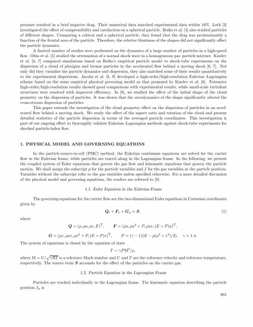
To underscore that the flow dynamics of a rectangular cloud at moderate angles are comparable to that of a

triangle, we place a square cloud (η = 1) under an angle of rotation θ = 45◦. The front half of the diamond shape is

now geometrically exactly a triangle. From the snapshots at early times (Figs. 10a and 10b) and late times (Figs. 10c

and 10d), we can see that the dynamics of this front half is indeed the same as that of the triangle described above.

909

(c) (d)

x

y

0.4 0.8 1.20x

y

0.4 0.8 1.20

_0.2

_0.4

_0.6

0.6

0.4

0.2

0

_0.2

_0.4

_0.6

0.6

0.4

0.2

0

(a) (b)

x

y

0.2 0.4 0.6

_0.1

_0.2

_0.3

0.3

0.2

0.1

0

0 x

y

0.2 0.4 0.6

_0.1

_0.2

_0.3

0.3

0.2

0.1

0

0

Fig. 10. Velocity contours and particle dispersion patterns in a triangular cloud (a and c) and asquare cloud (b and d) at θ = 45◦: t = 0.3 (a and b) and t = 1.0 (c and d).

The trailing half of the diamond does not move significantly; as this half is shielded from the oncoming flow, it does

not significantly affect the gas flow at early times. At later times, the wider trailing half of the diamond is exposed

to the oncoming flow, yielding a slightly wider cloud and wake, as compared to the triangular case.

The square cloud is convected further downstream in the x direction at a zero angle of rotation θ = 0 than

at θ = 45◦, because the force between the gas and particle phase at is larger for the blunt square shape at zero

rotation as compared to the more aerodynamic rotated shape with θ = 45◦. Therefore, xdisp is larger at small angles

of rotation, as compared to moderate angles of rotation (Fig. 11a). Because of the symmetry of the square, the

xdisp(θ) curve is symmetric versus the angle of rotation θ. It should be noted again that the cloud with η = η∗ > 1

and θ = 90◦ is geometrically identical to the shape with η = 1/η∗ and θ = 0. The value of xdisp is smaller for η > 1

and θ = 0, as compared to that at θ = 90◦ (see Fig. 7). We observe that the curves for different aspect ratios in

Fig. 11a cross through a single point, indicating a correlation between rectangular clouds at θ ≈ 30◦. At moderate

angles of rotation, rectangles behave like triangles; hence, they show a minimum of ydisp(θ) for all η. The minimum

is naturally at θ = 45◦ for the symmetric square, and the compression of the cloud reduces with increasing η.

A comparison of the dependence for the ellipsoid cloud in Figs. 11 and 12 with that for the rectangular cloud

confirms the similarity between the two shapes. Figure 12a shows the same crossing at a single point of the curves

with different aspect ratios, only at a slightly smaller rotation angle θ = 15◦. As a circle with η = 1 does not change

geometrically with rotation, xdisp is not affected by the rotation angle θ.

For shapes with η > 1, instabilities play a major role in the dispersion of the particle clouds at late times,

which causes a disparity in the initial spanwise dispersion for a zero angle of rotation. Early flow dynamics dominates

the ydisp trends for clouds rotated past 45◦.

910

(à) (b)

1

4

2

3

1

4

2

3

ydispxdisp

_0.5

0

0.5

1.0

2.0

1.5

75604530150.1

0

0.3

0.2

0.6

0.4

0.5

75604530150

1

4

23

o, deg o, deg

Fig. 11. Dependences xdisp(θ) (a) and ydisp(θ) (b) for initially rectangular clouds: η = 1 (1), 2 (2),3 (3), and 4 (4).

(a) (b)

1

4

2

3

1

4

2

3

ydispxdisp

0

0.5

1.0

2.0

1.5

75604530150.45

0

0.55

0.50

0.75

0.65

0.70

0.60

7560453015o, deg o, deg

Fig. 12. Dependences xdisp(θ) (a) and ydisp(θ) (b) for initially ellipsoidal clouds: η = 1 (1), 2 (2),3 (3), and 4 (4).

CONCLUSIONS

A numerical study of the effect of the initial shape, aspect ratio, and rotation of a cloud of particles on the

particle-laden flow development in an accelerated flow behind a moving shock is conducted, using a high-order/high-

resolution Eulerian–Lagrangian method. A change in the cloud shape dramatically changes the particle-laden flow

development. In the case of an initially rectangular cloud, particles separate mostly along shear layers into distinct

arms that emanate from the front corners. These arms shield the rear part of the cloud from the incoming flow.

The flow separation location changes in time along the smooth circular cloud surface; hence, the particle arms are

less distinct, as compared to the initially rectangular cloud. The flow remains attached along the sides of the more

aerodynamically shaped triangular cloud, and particles are transported along shear layers that emanate from the

rear corners.

The averaged triangular cloud location is 40% less downstream, as compared to the blunt rectangular and

circular clouds at the time t = 1.0. This is attributed to reduced forcing between the gas and particle phase and,

hence, a smaller particle acceleration for the more aerodynamic triangular shape. The attached gas flow along

the sides of the triangular shape compresses the particles toward the symmetry line, leading to reduction of the

911

root-mean-square cross-stream location of the cloud. The particles that are pulled out of the rectangular and

circular shapes by separated shear layers move away from the symmetry line and increase the root-mean-square

cross-stream cloud location. A change in the aspect ratio (η) does not change the particle-laden flow qualitatively.

However, a slender, more aerodynamically efficient cloud is convected less in the streamwise direction, as compared

to low,aspect,ratio shapes. Clouds with smaller values of η are relatively more compressed in the streamwise

direction, whereas high-aspect-ratio shapes are relatively more compressed in the cross-stream direction.

Except for small wake and dispersion asymmetries, qualitative flow developments at small angles of rotation

are similar to the case of a zero angle of rotation. At moderate angles of rotation, the flow characteristics of the cases

with rectangular and ellipsoidal clouds are comparable to the flow features of the initially triangular cloud case.

The current investigation is part of a larger effort to validate our high-order/high-resolution

Eulerian–Lagrangian solver against shock-tube experiments.

We gratefully acknowledge the support of this work by the AFOSR contract No. G00008044 and by the

California Space Grant Consortium. The fourth author (Don) also would like to thank the support provided by

the Research Grant Council (Grant Nos. HKBU200909 and HKBU 200910 from the University Grant Council

of Hong Kong).

REFERENCES

1. V. Boiko and S. Poplavsky, “Particle and Drop Dynamics in the Flow behind a Shock Wave,” Fluid Dyn. 42,441–443 (2007).

2. M. Sun, T. Saito, K. Takayama, and H. Tanno, “Unsteady Drag on a Sphere by Shock Wave Loading,” ShockWaves 14, 3–9 (2004).

3. E. Loth, “Compressibility and Rarefaction Effects on Drag of a Spherical Particle,” AIAA J. 46, 2219–2228(2008).

4. V. Boiko and S. Poplavsky, “Dynamics of Irregularly Shaped Bodies in a Flow behind a Shock Wave,”C. R. Mecanique 332, 181–187 (2004).

5. M. Olim, G. Ben-Dor, M. Mond, and O. Igra, “A General Attenuation Law of Moderate Planar Waves Prop-agating into Dusty Gases with Relatively High Loading Ratios of Solid Particles,” Fluid Dyn. Res. 6, 185–199(1990).

6. V. P. Kiselev, S. P. Kiselev, and V. M. Fomin, “Interaction of a Shock Wave with a Cloud of Particles of FiniteDimensions.” J. Appl. Mech. Tech. Phys. 35 (2), 183–192 (1994).

7. B. Boiko, V. Kiselev, S. Kiselev, et al., “Interaction of a Shock Wave with a Cloud of Particles,” Combust.,Expl., Shock Waves 32, 191–203 (1996).

8. G. Jacobs and W. S. Don, “A High-Order WENO-Z Finite Difference Based Particle-Source-in-Cell Method forComputation of Particle-Laden Flows with Shocks,” J. Comput. Phys. 228 (5), 1365–1379 (2009).

9. G. Jacobs, W. S. Don, and T. Dittmann, “High-Order Resolution Eulerian–Lagrangian Simulations of ParticleDispersion in the Accelerated Flow behind a Moving Shock,” Theor. Comput. Fluid Dyn. 26 (1–4), 37–50(2010).

10. C. W. Shu, “High Order Weighted Essentially Non-Oscillatory Schemes for Convection Dominated Problems,”SIAM Rev. 51, 82–126 (2009).

11. D. Balsara and C. W. Shu, “Monotonicity Preserving Weighted Essentially Non-Oscillatory Schemes withIncreasingly High Order of Accuracy,” J. Comput. Phys. 160, 405–452 (2000).

12. M. Latini, O. Schilling, and W. S. Don, “Effects of Order of WENO Flux Reconstruction and Spatial Resolutionon Reshocked Two-Dimensional Richtmyer–Meshkov Instability,” J. Comput. Phys. 221, 805–836 (2007).

13. Z. Gao, W. S. Don, and Z. Li, “High Order Weighted Essentially Non-Oscillation Schemes for One-DimensionalDetonation Wave Simulations,” J. Comput. Math. 29, 623–638 (2011).

14. Z. Gao, W. S. Don, and Z. Li, “High Order Weighted Essentially Non-Oscillation Schemes for Two-DimensionalDetonation Wave Simulations,” J. Sci. Comput. 53 (1), 80–101 (2012).

15. R. Borges, M. Carmona, B. Costa, and W. S. Don, “An Improved Weighted Essentially Non-Oscillatory Schemefor Hyperbolic Conservation Laws,” J. Comput. Phys., No. 6, 3101–3211 (2008).

16. M. Castro, B. Costa, and W. S. Don, “High Order Weighted Essentially Non-Oscillatory WENO-Z Schemes forHyperbolic Conservation Laws,” J. Comput. Phys. 230, 1766–1792 (2011).

912