mathematics of dispersion with linear adsorption isotherm · mathematics of dispersion with linear...

Mathematics of

Dispersion With Linear

Adsorption IsothermGEOLOGICAL SURVEY PROFESSIONAL PAPER 411-H

Mathematics of

Dispersion With Linear

Adsorption IsothermBy AKIO OGATA

FLUID MOVEMENT IN EARTH MATERIALS

GEOLOGICAL SURVEY PROFESSIONAL PAPER 411-H

A theoretical consideration of the effect of a reacting

media on the dispersion of fluids in porous media

UNITED STATES GOVERNMENT PRINTING OFFICE, WASHINGTON : 1964

UNITED STATES DEPARTMENT OF THE INTERIOR

STEWART L. UDALL, Secretary

GEOLOGICAL SURVEY

Thomas B. Nolan, Director

The U.S. Geological Survey Library has cataloged this publication as follows:

Ogata, Akio 1927-Mathematics of dispersion with linear adsorption isotherm.

Washington, U.S. Govt. Print. Off., 1964.

iii, 9 p. diagrs. 30 cm. ,(U.S. Geological Survey. Professional paper 411-H)

Fluid movement in earth materials. Bibliography: p. 9.

1. Dispersion. 2. Adsorption. I. Title. (Series)

For sale by the Superintendent of Documents, U.S. Government Printing OfficeWashington, D.C. 20402

CONTENTS

PageAbstract._ _________________________________________ HIIntroduction _______________________________________ 1Adsorption isotherms..._____________________________ 1Field equation____________________________________ 2Review of some previous analyses___________________ 3Mathematical analysis_____________________________ 4Special situations-____________________________-_-___ 7Discussion _________________________________________ 8References _________________________________________ 9

ILLUSTRATIONS

Page FIGURE 1. Concentration distribution for system with irreversible linear adsorption isotherm.__________--_--__---------_ H4

2. Plot of /-function____________________________________________________________------------_----------- 7

SYMBOLS

Di Dispersion coefficient in the direction i; i=x, y, z.O Concentration of the liquid phase.(70 Concentration of the liquid at a given point, say, o?=0.N Concentration of the solid phase.NQ Concentration of the solid phase at saturation.k, m Constants associated with adsorption isotherm.u Average velocity of the liquid.t Time variable.x Space variable.A Integration constant.I0 (x) Modified Bessels function of the first kind of order zero.J0 (x) Bessels function of the first kind of order zero.erfc (a;) Complementary error function.J(x, y) Goldsteins J-function.L<t>(£) Laplace transform of functionL~l<j>(p) Inverse Laplace transform.U(t h} Unit step function.a a2/32&2m/4£2 or a2/32&2m/4.b ap/2.a UX/2D.

Dummy variable.in

FLUID MOVEMENT IN EARTH MATERIALS

MATHEMATICS OF DISPERSION WITH LINEAR ADSORPTION ISOTHERM

By AKIO OGATA

ABSTRACT

The simultaneous occurrence of dispersion and adsorption is noted frequently in laboratory models. In most investigation, especially that of the exchange process, the adsorption phase dominates; thus, prediction is based on a reduced system. The discussion presented in this paper, however, is based on the concept that the orders of magnitude of the adsorptive and the dispersive processes are the same. In addition, because of the meager knowledge of the macroscopic adsorption, the isotherm is assumed to be linear. This leads to a system which may be described by the equations

nda;2 U do;

The paper deals entirely with the solution of the above equations for flow in a porous column.

INTRODUCTION

In the transport of two miscible fluids through isotropic porous media, the mixing and the dilution of any contained contaminant is dependent on two mechanisms, namely, mechanical dispersion and adsorption. The mechanical dispersion is defined to include all mechanisms that tend to cause spreading of the fluid stream which generally arises because of variations in fluid velocity throughout microscopic segments of the porous medium. Although variations in the magnitude and direction of the fluid velocity is noted throughout macroscopic segments of heterogeneous materials, the theory of dispersion cannot be extended to describe this system. The adsorption mechanism is defined as the removal or addition of the contained contaminant by the solid matrix through which the fluid flows. That is, the solid material may be thought to act as a mathematical source or sink depending on the concen tration of the liquid flowing through the porous medium.

The physicochemical aspects of the problem of adsorption are generally approached through thermo- dynamic principles based on analysis of the total free

energy available at any given state. However, because of the complexities of these phenomena and the porous medium, such analysis has as yet produced no general conclusions on how to make use of the adsorption isotherms that characterize naturally occurring porous media. In other words, because of the extreme range of conditions met in aquifers, adsorption study of small segments of the flow system microscopic analysis has not produced results directly applicable to the entire flow regime. This indicates that for each soil complex or aquifer material, the adsorption characteristics of various candidate tracer materials must be predeter mined so that the results can be given macroscopic application.

To circumvent this difficulty, most quantitative analyses of laboratory experiments are generally based on an assumed adsorption isotherm. In most situa tions the tracer or contaminant concentration is suf ficiently small that a linear isotherm can be assumed. This is the condition on which the following analysis is based. Adamson (1960), however, discussed various findings of recent years in which the linear assumption does not hold, especially where high concentrations are reached. Because in both laboratory tracer studies and actual disposal systems the concentrations are kept at a minimum, it is believed that the adoption of a linear isotherm is a reasonable approximation.

Linear isotherms have been utilized by chemical engineers in the study of exchange processes. There is, of course, no proof that the same type of isotherm would be applicable for adsorption in a nonactivated bed. However, for want of better or more detailed informa tion, the assumption of a nonlinear isotherm would only increase the mathematical complexity without furthering the systematic progress of the investigations.

ADSORPTION ISOTHERMS

A linear isotherm under isotropic exchange conditions may be generally classified as representing either a

HI

H2 FLUID MOVEMENT IN EARTH MATERIALS

reversible or irreversible reaction. The simplest situa tion is the linear isotherm which represents an irrevers ible system, as described by the expression

(1)

where N is the solid-phase concentration defined as the mass per unit volume of solid material, C is the liquid- phase concentration defined as the mass per unit volume of liquid, t is the time variable, and k is the proportional ity constant. Equation 1 is essentially Langmuir's isotherm for low concentrations and for equilibrium conditions. For complete discussion of Langmuir's isotherm, the reader is referred to Adamson (1960). It is noted that equation 1 describes a system in which the solid acts as a mathematical sink. That is, the amount transferred or the rate of change of solid concentration with time depends only on the liquid concentration. Physically this system cannot exist unless some method is available to remove all material transferred from the liquid to the solid phase. In terms of the overall mathematical treatment, however, inclusion of the terms represented in equation 1 does not add to the complexity of the problem.

More generally, isotherms of this nature may be expressed as

. -^r=F(O (2) * ot

where F(C] is a function of liquid concentration only and must be determined for each system considered.

In all situations, the medium tends to show a fixed capacity to adsorb a given substance which in turn is set by the level of the liquid concentration. That is, dN/dt becomes zero, indicating establishment of equi librium between the liquid- and the solid-phase con centrations. An example of this type of isotherm is that used by Amundson (1948), mathematically rep resented by the equation

(3)

In equation 3, a is a constant and NQ is the saturation capacity of a unit volume of granular material. It is noted that equation 3, like equation 1, shows a straight- line relation within the range of the porous medium's capacity to adsorb. The saturation capacity N0 is dependent on the concentration of the liquid phase and thus is assumed to be a known constant in any given analytical study.

Merriam and others (1952) and Hougen and Mar shall (1947) indicated that the adsorption isotherm can be depicted by the expression

bN=k(C-mN) (4)

where m is a constant. Note that unlike equation 3, equation 4 indicates a possible negative rate of change of solid concentration. This indicates that the ad sorption process is reversible in the sense that when mN ^> C the rate of change is negative, hence providing for a reverse effect or diminution of the solid-phase con centration. In other words, in a continuous-injection system, a continuous adsorption and desorption process is possible.

The problems in which adsorption has been investi gated extensively are those involving gas or liquid flow through activated porous media. There is general agreement that the dispersion under these conditions is so small that it may be neglected in describing the outflow-concentration profile. This assumption elimi nates the second-order term in equation 5 and the mathematical treatment is thereby simplified to some degree. In a liquid-solid system, for the conditions imposed in waste-disposal problems, the relative magnitudes of the two processes are not known. It appears that, for the initial passage of the contami nant, the condition of dN/dt»D(&C/dx2) would be valid. However, under conditions of repeated injec tion, the available free energy may be reduced to a great extent by the preceding injection; hence, the relative magnitudes may be of the same order. The immediate significance of this relates to the predicting of the usefulness of any given analysis, in that the historical events may figure importantly in evaluating the fate of the contaminant.

In the following analysis the isotherm described by equation 4 is utilized. This assumption admittedly restricts the applicability of the resulting analytical solution, but our knowledge is too meager to specify these limitations. It is believed that, as more data become available, the applicability of the solution will become more clearly defined.

FIELD EQUATION

The actual description of mass transport through porous media is a matter of conjecture since there is no method available to measure all energy states of the system. The differential equation presented is thus based on a macroscopic concept so that the primary result gives a description of the liquid-concentration distribution at a given point in space for a given time. The mathematical model considered is that of flow through a column of semi-infinite extent. It is, thus, assumed that

(a) porous medium is homogeneous and isotropic, (6) flow field is parallel to the x axis (say), and

MATHEMATICS OF DISPERSION WITH LINEAR ADSORPTION ISOTHERM H3

(c) mass-transfer rate from liquid to solid is linear and can be expressed by equation 4 that is,

Assuming that the three components of mass trans port are dispersion, convection, and adsorption, the law of conservation of mass may be stated as

(5)

where the relationship between 2V and C is given by equation 4 and the transport due to dispersion is de scribed by an equation similar to Fick's law in a moving medium that is, the total transport is

.x ~ x bz

The symbols appearing or inherent in equation 5 are defined as follows:

D: dispersion coefficient, u: average velocity or interstitial velocity,

k, m: constants relating the adsorption isotherm, C: concentration of the liquid phase, N: concentration of the solid phase, x: space variable, and t: time.

The boundary conditions chosen are parallel to those of other investigators. Say, at x=0, the liquid concentration is maintained at some constant value, 0 C0 . This condition depicts dispersion phenomena from a plane source discharging into a semi-infinite medium. Mathematically, these boundary conditions can be stated:

and lim C(x, 0 = 0forz *a>

N(x, 0) = 0for z>

(6)

Before developing an analysis of equation 5, subject to conditions 6, it will be of interest to review other solu tions obtained in the analysis of exchange phenomena.

REVIEW OF SOME PREVIOUS ANALYSES

Amundson (1948), in describing the mass transport, assumed that dispersion is small; hence, equation 5 becomes

where a is the volume of voids in the medium. The assumed adsorption isotherm is given by equation 3. The boundary conditions are as specified in 6, except for the condition N(x,Q)=Ni(x). For this system, the solution obtained is

u ^x> l> ~ t pO-z/u) -| ka I Co(ij)dij I

(if r* ̂ j= f(t-x/u) =j ' f [No-Ni(&] d£ + exp ka\ C0 (rfdi, \-l

l»Jo J L Jo Jexp

which is valid for Z> x/u. Because dispersion is neglected, it is noted that N(x,t)=Ni(x) for t < x/u, which means that no transfer from liquid to solid occurs until mass is transported by convection to the point of interest. Because the solution is given in terms of functions of the coordinates, there is no immediate applicability unless these functions are defined.

A special circumstance considered by Amundson is for the conditions dCy&«dN/& and #,(») = N(x, 0)=0. These assumptions may be interpreted to mean that the convective transport is large enough to balance the amount adsorbed; thus ~bCj~bt remains small. For this special circumstance, the solution reduces to

exp

Of specific interest is the analysis of Hougen and Marshall (1947), who considered the isotherm ex pressed by equation 4. However, the authors con sidered only the special circumstance where dispersion is negligible and dCydi«d2V/di. Thus, equation 5 can be written, simply,

bC 1 bJV"u at

The solution of this system subjected to the boundary conditions specified by 6 is

(7 fkx/u7r = l exp ( kmt) exp ( Oo Jo

where J0 (z) is the Bessel function of the first kind of order zero. This equation has been calculated extensively and was discussed by Marshall and Pig- ford (1947).

Because exchange phenomena are of primary interest in chemical processes and the significant aspect of this application is limited to the condition where adsorption is of much greater magnitude than dispersion, scientific interest has tended to remain centered around the previously discussed situations. However, there ap pears to be one situation for which a solution of equation 5 has been obtained. This is the most simple condition of a linear irreversible isotherm, which is given by equation 1. Analysis of this system is analogous to solving the heat-conduction equation with radiation at the boundary. The solution, as determined for example by the writer ("Dispersion in Porous Media,"


£ = ut/x

FIGURE 1. Concentration distribution for system with irreversible linear adsorption isotherm.

doctoral dissertation, Northwestern Univ., 1958), has the form

C 1 ,.. ,-M) erfc

exp

l-.*j/) * ~|* /2VZ>U

ux~\ , r/,. ut9n erfc I 1+ 2£>J L\ a;

where M= CJj VThe adsorption term ^ intro-

otduces a "holdup time" and sets an upper limit to C/CQ depending on the value of k. For example,

does not correspond to the point t as indicated byusolution of the dispersion equation when Ar=0. In addition, the slope of the effluent curve with respect to time is smaller and an upper limit other than <7/(70=l is reached because of the continual removal of sub stance from the system. The effect of the adsorption

4y/y»

term L> shown in figure 1 for the special case of 17=-=-=1.

Crank (1956), on the other hand, gave a solution of equation 5 for u=Q, using the isotherm depicted by equation 4. In his discussion he cited situations of diffusion in a plane sheet and in a cylinder. The

solutions are, however, too complex to be discussed in this paper. Interested persons are referred to Crank's book, in which a complete discussion of numerical computation and solution in graphical form is presented.

MATHEMATICAL ANALYSIS

Let us consider now the dispersion and adsorption phenomena utilizing equations 4 and 5, subject to con ditions 6. There are various analytical methods that can be employed to obtain the solution of the differential equation. However, for this type of problem perhaps the simplest and most straightforward method is that employing the operational device called Laplace trans forms. Because of its usefulness in analysis, various texts have been written on the theory and application of the Laplace transform. For discussion and applica tion of complex variables and transform calculus, the reader is referred to McLachlan (1955), Churchill (1958), or Doetsch (1961). _

The Laplace transform C(x, p) is defined by the expression

/ CO

V(x,p)=\ e-Jo

Hence, substitution of the integral transform into equa-


tions 4 and 5 gives the expressions

andHx*~ u dx = (7)

(8)

It is noted that the transformation reduces the second- order partial differential equation into a second-order ordinary differential equation and reduce^ the first-order equation to an algebraic equation.

In establishing equations 7 and 8, two of the bound ary conditions, C(x, 0)=0 and N(x, 0)=0, have been utilized. The remaining two boundary conditions written in terms of G are

andlim 17=0.

The simultaneous equations 7 and 8 may be readily solved^ by solving for N in equation 8 and substituting for N in equation 7. This process gives a single equation,

n d*V dV A , * \D -r-^ u T~=P ( 1+ rr~ )dx2 dx * \ p+km/

The resulting equation is a linear second-order ordi nary differential equation with constant coefficient for which the solution can be readily obtained. The com plete solution is

Application of the boundary conditions specifies that since C( <» , p) =0, only the negative part of the argument is retained, and since C(Q,p~) = CQ/p} A=C0/p. Thus, the required solution of the transformed system is

r -p {& [- (9)

The initial step hi determining the inverse transform is to refer to any table of inverse Laplace transforms for example, Erdelyi and others (1954). If the required V does not appear in the tables, the inversion theorem is utilized which states that

C(x, f)=~ (10)

where r specifies a given path in the complex plane z. The choice of r is dependent on the singular points of the function given in equation 9 (McLachlan, 1955). The function involved does not, however, lend itself for ready determination of the type of singularity involved in the computation. Hence, the following mathematical manipulation is a process of simplification so that

732-758 64 2

various theorems in conjunction with a table of inverse transforms may be utilized to obtain the desired results.

From any table of integration, it is noted that

A r v» J°

Hence, equation 9 can be written in terms of an infinite integral to eliminate the radical term that is,

where a=ux/2D and ^2 == _ Accordingly assuming C is continuous, substituting C

into equation 10 leads to the expression

where p is replaced by z.Let us consider only the complex part and denote this

by the symbol F. Letting (z+km)=\, the complex part can be written

El __g-kmt

2W L exp [A*-

Rearranging the argument of the exponential term, the expression can be written

r a3ai ~\ i F=exp I kmt -TTJ (k krn) 5 .

f P\ (t «2 /32\ i c?fPk*m~\ d\ Jr eXP L V "4FV + 4£*X J \-krn

Thus, the complex part of the function F is

dxX km (11)

The nature of equation 11 makes further simplifica tion possible by the use of the shift theorem (McLachlan, 1955). The shift theorem specifies that if there exists a function defined as

where X(£) is continuous or piecewise continuous for t^>h, its transform is obtainable by the standard method. The value of the integral, however, is zero when £< h, which indicates physically a moving system or in this circumstance signifies that the concentration is zero until the contaminant arrives at the point hit.


It is again noted that the Laplace transform is de fined by

Keplacing (t) in the above expression by (t h) gives

= f e-*'-v<t>(t-h)dt=ert f°Jh Jk

= f°° e~^<}>(tv 0

where U(t h) is a unit step function with properties U=0 for t<^h and C7= 1 for t^>h. The inversion of this function can be written symbolically as

L-le-rt$(p)=<t>(t-h} U(t-h).

Thus, if !j>(p) exists, the inverse transform of ^(t h) can readily be obtained since L~l ^>(p) = 4>(t) .

In this specific problem, the function for which the inverse must be determined is

exp

As previously stated, L~1 ^(p)~^(t); hence, the re quired computation can be written in operational form,

where a2=a2/32A:2m/4f .Because the exact expression of $ does not appear in

tables of inverse Laplace transforms, the function is rewritten

= exp (o2/p) + exp (o'/p).

Each term in the function 0 can then be directly ob tained from the table of inverse Laplace transforms that is,

Ir1 exp (o2/p)/p=/o(2aVO and

L-U/(p+5)=exp(50.

Thus, the first term of 0(£) is I0 (2a-Ji). The second term, on the other hand, can be evaluated from the con volution or superposition theorem which states that if Lf(t)=J(p) and Lg(t) = H(p), then

= P/(r)<7(«-r)dT= PJo Jo

Hence, the second term can be shown to be

p kmQ2/P p

P ~"Jfl

The function <$>(t) thus can be written

t P e-* Jo

Further, letting a=a/%, where a=a2^2k2m/4:} the shift theorem requires that the inverse of equation 11 be written

n] Jo

(12)

equation 12 is valid for £>62/£2 where &2=a2j82/4. Since the solution gives zero values for i<a2jS2/4^2, or/#2 \ / £<j j^ j /^2, the particular solution of equations 4 and 5,

subject to conditions 6, becomesn Opa /*^=^=Co YOT- JZ

jexp [-

+exp (

exp

(13)

where a=ux/2D and 72 =/32a2/4=z2/4#.Equation 13 cannot be simplified; however, it can be

written in terms of a tabulated function J introduced by Goldstein (1953). A complete discussion of the various properties of the J-i unction was given by Goldstein. The function is defined by

=e-« fV< Jo

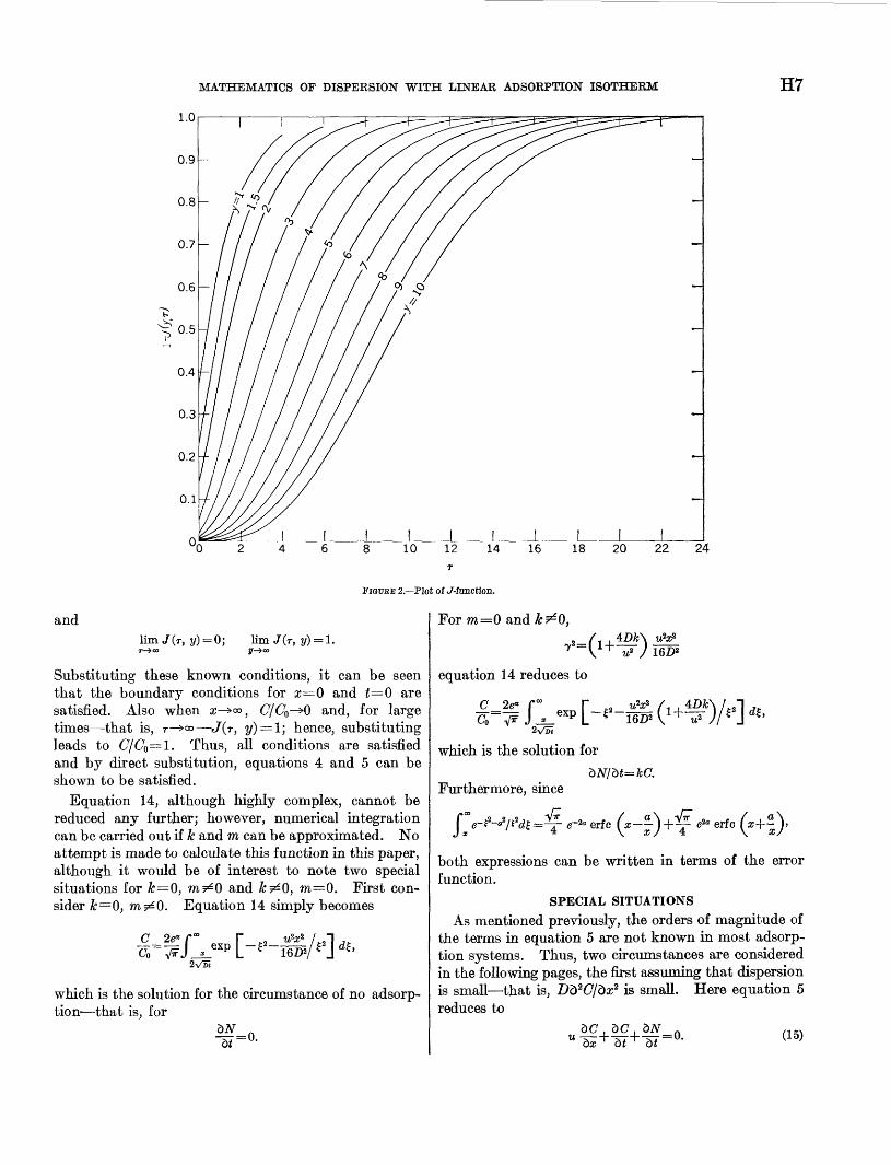
The function J(x, y) appears in a wide variety of prob lems and therefore no attempt is made to list its prop erties. The reader is referred to Luke (1962), who listed the more significant properties, or to the original work of Goldstein. Luke also listed some of the com puted tables of the J-function appearing in various publications. To illustrate J(x, y), the function com puted by the writer is presented in figure 2.

Noting that one of the elementary properties of this function is

J(r, y~)+J(y, T)-l=e-<'+»>/0 (2V^)

and utilizing the definition of the J-function, equation 13 can be written

C_ = 2e« r Co vV J

(14)

where y=ky2/£2 and T=km(t y2/%2').To determine whether the boundary conditions are

satisfied, it is noted that

/(O, i/) = /(r,0)=e-'

MATHEMATICS OF DISPERSION WITH LINEAR ADSORPTION ISOTHERM

i. Gi

FIGUBE 2. Plot of J-function.

andlim lim J(T, y) =

Substituting these known conditions, it can be seen that the boundary conditions for x 0 and t=0 are satisfied. Also when x ><*, C/C0 >0 and, for large times that is, r >Q° J(r, y) = l', hence, substituting leads to C/C0 =1. Thus, all conditions are satisfied and by direct substitution, equations 4 and 5 can be shown to be satisfied.

Equation 14, although highly complex, cannot be reduced any further; however, numerical integration can be carried out if k and m can be approximated. No attempt is made to calculate this function in this paper, although it would be of interest to note two special situations for k=Q, m^Q and k^Q, m Q. First con sider k=0, m^O. Equation 14 simply becomes

_cCo"

2v/5i

which is the solution for the circumstance of no adsorp tion that is, for

For m=0 and_7 "_/ 4Z)fc\ "

equation 14 reduces to

C 2e« f 00 Ta^v^ J ^_ exp2Vci

which is the solution for

Furthermore, since

= e-^ erfc *- + e20 erfc

both expressions can be written in terms of the error function.

SPECIAL SITUATIONS

As mentioned previously, the orders of magnitude of the terms in equation 5 are not known in most adsorp tion systems. Thus, two circumstances are considered in the following pages, the first assuming that dispersion is small that is, Z>d2(7/dz2 is small. Here equation 5 reduces to

dC bC, c)2V_ ~ ~~ (15)


Second is the circumstance where d(?/d£<CdAYd£, thus reducing equation 5 to

_ _ U ~ (16)

The mass transfer to the solid phase is again assumed to be expressed by equation 4 and the boundary conditions are those given in 6. The conditions under which these assumptions are valid are not known; however, these solutions may be useful in analyzing some laboratory models.

For both circumstances expressed by equations 15 and 16, the method utilized is the Laplace transformation. Hence, applying the Laplace transform to equation 15, the subsidiary equations obtained are

u -r--\-pC-}-pN=

andPN=k(C-mN)

#=(n

V) J

(17)

Equations 17 are now first-order differential equations with constant coefficient; the solution can be shown to be

u p -\-krn

From the initial condition C(x, 0) = <70 f or £>0, the constant A is again determined to be

A=Co/p.

Further, letting s=p+km and utilizing the inversion theorem, the solution can be expressed

-kmt-(k-km)- dz

Or,dz

Accordingly, utilizing the shift theorem, the function for which the inverse is to be determined is

_k*mx , / e u ''/ (s-km).

The transformation is carried out in the same manner as that used in obtaining equation 14. The required solution is, thus,

m f ,-x\ kr t r IJfZ / ^\TI * I IT I n /'"' *' 1 / j ** 1 IV u) u iI0 2-\ km [ t )

I L V u V «/ J

-{-km exp j km (t ^

c7T Co

for t^>x/u. The above relation written in terms of the previously described J-fimction is simply

7r=J(y, (18)

kx / x\ where y= and r=km (t ). Equation 18, iny u \ «/

terms of a definite integral, can be writtenr -km(t-~* *-> -i \

It is noted that the function obtained above is the same as that derived by Hougen and Marshall with the

replacement of f t J for t. This function has been

computed and is presented in graphical form as figure 2.3/Further, note that for £«-, equation 19 reduces to' u' n

~ = e-kx/u rt K >Co

which indicates that measurable traces of solute will appear at t=x/u provided k is small. In most experi mental setups, the holdup time is much greater; thus the expression is generally not useful in the analysis of experimental data.

Let us consider now the second special circumstance in which dN/<)t^>dC/dt. Here the transformed or the subsidiary equations become

dC «

and

Solving for U gives

exp -

The inverse obtained in the same manner described previously is

?

+ kme *»"

where @=Dka2/u2.In terms of the J-function, the preceding relation

becomesC_ =2e^ fCo V^ Jo

exp [-!2- (20)

where y=P/£2 and r=kmt. However, once again the function is not reducible and in its integral form can be written

~Co

exp ^-r

^o(21)

DISCUSSION

To effectively predict the fate of a tracer or contami nant as it progresses through porous material, two phenomena must be predicted beforehand. These consist of dispersion due to departures from the flow


predicted by use of Darcy's law and the loss of material through adsorption by the porous medium. The first effect can generally be predicted for laboratory condi tions, because flow is controlled to fit the theoretical conditions postulated. The adsorption effect, on the other hand, cannot be controlled even under conditions met in the laboratory. It can only be said to be dependent on the tracer and the soil constituents.

Because of this unknown factor that inevitably appears in all types of studies involving tracers, the need for finding a near-perfect tracer is apparent. But discovery of this near-perfect tracer is yet to be made, although there appear to be a few elements that display only minor attraction to the silica sands commonly used in the laboratory. However, when natural soils are used as the porous medium, adsorption may play an important role in determining the distribution of tracer material at some point downstream. This then requires that the laboratory data be analyzed to esti mate the rate at which the tracer or contaminant is transported from the liquid to the solid. Studies of exchange processes show that, in the low-liquid-con centration range, a good approximation is obtained by assuming a linear adsorption isotherm.

On the basis of these findings the preceding mathe matical analyses were developed utilizing the linear isotherm described by equation 4. The solutions obtained are extensions of previous expressions which were developed and used to represent ion-exchange phenomena in fixed columns. However, the final solu tions, equations 14, 18, and 20, are such that no real purpose would be accomplished by numerical computa tion unless realistic values of k and m in equation 4 were available.

It is expected that, as some data indicating the range of k and m become available, computation of equation 14, 18, or 20 will be attempted. From the experimental and analytical standpoint, equation 18 would be the most appropriate for obtaining an approxi mation of the constants k and m, provided extremely slow flow can be obtained in the experimental model.

REFERENCES

Adamson, A. W., 1960, Physical chemistry of surfaces: NewYork, Interscience Publishers, 629 p.

Amundson, Neal R., 1948, A note on the mathematics of adsorp tion in beds: Jour. Physical and Colloidal Chem., v. 52,no. 10, p. 1153.

Churchill, Ruel V., 1958, Operational mathematics: New York,McGraw-Hill Book Co., 331 p.

Crank, J., 1956, The mathematics of diffusion: London, OxfordUniv. Press, 347 p.

Doetsch, Gustav, 1961, Guide to the application of Laplacetransforms: New York, D. Van Nostrand Co., 255 p.

Erd&yi, Arthur, Magnus, Wilhelm, Oberhettinger, Fritz, andTricomi, F. G., 1954, Table of integral transforms, vol. I:New York, McGraw-Hill Book Co., 391 p.

Goldstein, S., 1953, On the mathematics of exchange processes infixed columns: Royal Soc. (London) Proc., v. 219, p. 151.

Hougen, O. A. and Marshall, W. R., 1947, Adsorption from afluid stream flowing through a stationary granular bed:Chem. Eng. Process, v. 43, no. 4, p. 197.

Luke, Yudell L., 1962, Integrals of Bessels functions: New York,McGraw-Hill Book Co., 419 p.

Marshall, W. R., Jr., and Pigford, R. L., 1947, Application ofdifferential equations to chemical engineering: Newark,Del., Univ. Delaware Press, 135 p.

McLachlan, N. W., 1955, Complex variable theory and trans form calculus: London, Cambridge Univ. Press, 388 p.

Merriam, C. Neale, Jr., Southworth, Raymond W., and Thomas,Henry C., 1952, Ion exchange mechanism and isotherms fromdeep bed performance: Jour. Chem. Physics, v. 20, no. 12,p. 1842.

O