dislocation theory for engineers: worked...
TRANSCRIPT
Dislocation Theory for Engineers:Worked Examples

Dislocation Theoryfor Engineers:
Worked Exalllpies
Roy Faulknerand
John Martin

Book 744First published in 2000 by10M Communications Ltd1Carlton House Terrace
London SW1 Y 5DB
© 10M Communications Ltd 2000All rights reserved
10M Communications Ltdis a wholly-owned subsidiary of
The Institute of Materials
ISBN 1-86125-124-6
Typeset in the UK byKeyset Composition, Colchester
Printed and bound in the UK atThe Alden Press, Oxford

Acknowledgements
To my wife (Linda) for putting up with my enthusiasm for things which she regardswith lower priority. (RGF)
I am indebted to my colleagues at the Oxford University Department of Materialswho have provided a number of the numerical problems quoted in the text. I am alsomost grateful to Professor Brian Cantor FREng for the facilities provided for me inthe Department, and to Peter Danckwerts for his efficient dealing with editorialmatters. (JWM)
v


ContentsIntroduction IX
1 Dislocations in Pure Materials 1
The stress required for plastic yield in a single crystal 1Example 1.1 Identification of active slip system 1
The relative energies of defects formed by vacancy condensation 4Example 1.2 Frank loop and prismatic loop 4Example 1.3 Frank loop and tetrahedral defect 5
The effect of point defects on plastic flow 5Examp le 1.4 Chemical stress 6
The effect of other dislocations on plastic flow 7Example 1.5 Dislocation density 7Example 1.6 Average plastic shear strain 7Example 1.7 Forest model of flow stress 8Example 1.8 A parabolic stress-strain relationship 9
States of work hardening 10Example 1.9 Model of Stage I work hardening 11Example 1.10 Neutron irradiation hardening 12
Dislocation/grain boundary interactions-the Hall-Petch equation 14Example 1.11The Hall-Petch relationship (1) 15Example 1.12 The Hall-Petch relationship (2) 16
2 Dislocation Interactions in Single Phase Materials 19
Segregation of solute atoms to dislocations 19Example 2.1 The maximum temperature of segregation 19Example 2.2 Solute interaction with an edge dislocation 20Example 2.3 The rate of strain ageing 21
Dislocation dynamics of yielding 22Example 2.4 Upper and lower yield points 23
Strengthening by substitutional solute atoms 25Example 2.5 The CRSS for a crystal containing a random array of
point obstacles 25Example 2.6 Solute hardening in steel 28
vii

Contents
3 Dislocation Interactions in Two-Phase Alloys 31
Particle shearing by dislocations 31Example 3.1 Chemical strengthening 32Example 3.2 Stacking-fault strengthening 33Example 3.3 Coherency strengthening 34Example 3.4 Order hardening 34
Particle by-pass by dislocations 35Example 3.5 Effect of particle spacing on yield stress 35Example 3.6 Calculation of critical interparticle spacing 36
Combination of strengthening processes 37Example 3.7 Combining grain-size, solute and particle strengthening 37
4 Effects at Elevated Temperatures 41
Recovery and recrystallisa tion 41Example 4.1 The driving force for sub grain growth 42Example 4.2 Energy released during recrystallisation 43
Dislocation climb 45Example 4.3 Rate of annihilation of dislocation loops 45
Dislocation creep 47Example 4.4 Recovery creep model 49Example 4.5 Power law creep calculation 50Example 4.6 Use of the Monkman-Grant equation 51
5 Dislocations in Fracture Processes 55
Ductile fracture 55Example 5.1 Calculation of ductile fracture strain in a steel 56
The ductile-brittle transition 58Example 5.2 The effect of dislocation density on the ductile-brittle
transition 58Fa tigue fracture 60
Example 5.3 S-N curve prediction 64
viii

IntroductionOur application of elementary dislocation theory to the behaviour of crystallinematerials will be made systematically, as follows:
1. Pure materials, and the effect of lattice defects upon the behaviour ofdislocations, considering in turn point defects (vacancies), line defects (i.e.other dislocations) and planar defects (grain boundaries).
2. Solid solutions, considering the effects of the segregation of solutes todislocations, and also the interaction of moving dislocations with dispersedsolute atoms.
3. Two-phase materials, considering the interaction of dislocations with second-phase particles.
4. Elevated temperature effects, including recovery and recrystallization, as wellas dislocation creep.
5. Fracture processes including ductile fracture processes, the effect of disloca-tions at crack tips upon the ductile-brittle transition behaviour, as well asfatigue fracture properties.
We were commissioned to approach the subject in the form of a set of 'WorkedExamples' in order to complement the book of Worked Examples in Dislocations byM. 1. Whelan, which was published by the Institute of Materials in 1990.1 That bookprovides the essential basic concepts of dislocation theory, and the aim of thepresent text is to apply that elementary theory to a number of problems in materialsscience which should be of interest and value to the student reader.
The level is appropriate for that of the undergraduate student, and other, equallyappropriate introductory texts on the theory of dislocations in addition to that ofWhelan would be those by D. Hull and D. J. Bacon (Introduction to Dislocations, 3rdedition, Pergamon, 1995) and by 1. Weertman and 1. R. Weertman (ElementaryDislocation Theory, our; 1992).
There are several advanced texts on dislocation theory to which the graduatereader can turn. These include 1. P. Hirth and 1. Lothe (Theory of Dislocations 2ndedition, Krieger Publishing Co., 1992) and F. R. N. Nabarro (Theory of CrystalDislocations, Dover, 1987).
Finally, we include a list comprising a Glossary of the symbols employed in ourtext, and a list of the principal equations we have quoted without derivation:
b Burger's vectord grain size
ix

Introduction
D diffusion coefficientE Young's modulusE; dislocation core energy per unit lengthf volume fractionF obstacle strengthG shear modulusk Boltzmann's constantky slope of Hall-Petch plotKJ stress intensity (Mode I)iii Taylor factorM mobilityN, number of obstacles per unit areaN; number of obstacles per unit volumero inner cut-off radius from the dislocationt timeT line tension of dislocationw dislocation width
e tensile strainB strain ratel' shear strainI'SF stacking-fault energyv Poisson's ratiop dislocation densityU normal stresse work hardening rate'T shear stressn atomic volume
EQUATIONS1. Elastic field of a screw dislocation
U()z = Uz() = Gb/27Tr
2. Elastic stress field of an edge dislocation lying along the z direction with itsBurger's vector b lying parallel to x:
Uxx = - Dy(3x2 + y2)/(X2 + y2)2Uyy = Dy(x2 + y2)/(X2 + y2)2Uzz = v( Uxx + Uyy)uxy = Dx(x2 - y2)/(X2 + y2)2Uxz = uyz = 0
x

Introduction
where D = Gb/27T(1 - v), G is the shear modulus and v is Poisson's ratio.
3. Force per unit length acting on a dislocation (Peach-Koehler equation) = Tb.
. I h f . di I . E Gb2
I R4. Energy per unit engt 0 a screw IS ocation = e + -4- n-7T ro
Where Rand ro are the outer and inner cut-off radii respectively, and E; is the coreenergy per unit length.
5. Energy per unit length of an edge dislocation:
Gb2 (R)Ed = E; + 47T(1'- v) In ro
where E; is the core energy per unit length, Rand ro the outer and inner cut-offradius from the dislocation respectively.
xi

1Dislocations in Pure Materials
We will first consider the application of the Peach-Koehler formula, which is derivedin Whelan,! Ch. 5.
THE STRESS REQUIRED FOR PLASTIC YIELD INA SINGLE CRYSTAL
EXAMPLE 1.1 IDENTIFICATION OF ACTIVE SLIP SYSTEM
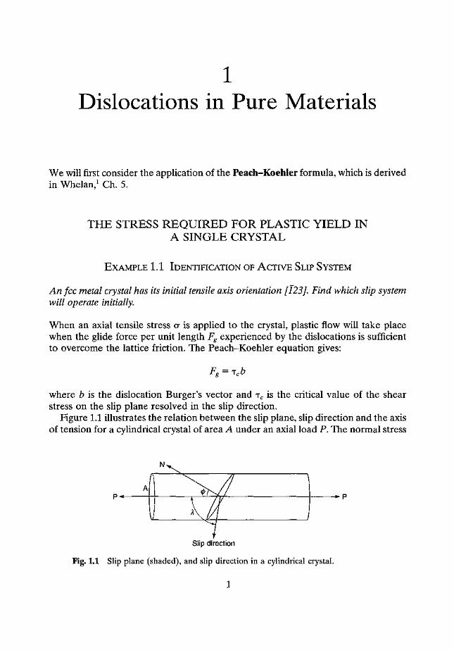
An fcc metal crystal has its initial tensile axis orientation [123J. Find which slip systemwill operate initially.
When an axial tensile stress (J" is applied to the crystal, plastic flow will take placewhen the glide force per unit length Fg experienced by the dislocations is sufficientto overcome the lattice friction. The Peach-Koehler equation gives:
where b is the dislocation Burger's vector and 1"c is the critical value of the shearstress on the slip plane resolved in the slip direction.
Figure 1.1 illustrates the relation between the slip plane, slip direction and the axisof tension for a cylindrical crystal of area A under an axial load P. The normal stress
Slip direction
Fig. 1.1 Slip plane (shaded), and slip direction in a cylindrical crystal.
1

Dislocation Theory for Engineers: Worked Examples
Fig. 1.2 Showing the relationship between the position of the tensile axis [123] andthe operating slip system (111)[101].
is (J" = PIA. If the angle between the slip plane normal and the tensile axis is <p, andthe angle between the slip direction and the tensile axis is A, then 'Tc may be readilyobtained. The component of the axial force P acting in the slip direction is P cos A;the area of the slip plane is A/cos <p, so:
'Tc = (J" cos Acos <p (1.1)
The operative slip system will be that for which the value of r in equation (1.1) is amaximum. The values of cos A and cos <p for each of the twelve slip systems of thefcc structure can be readily calculated by substitution in the 'cosine formula' forangles between plane normals in cubic crystals:
fcc crystals slip on {111]<110>, and the three <110> directions lying in each of thefour {111}planes may readily be written down, since the Weiss Zone Law states thatthe direction [UVW] lies in the plane (hkl) if
hU+kV+IW= 0
If a table of planes and directions is constructed, with the corresponding cos A andcos <p values, it will be seen that the operative slip system will be (111)[101], the valueof cos A cos <p being 0.4665.
Figure 1.2 illustrates on a stereogram the relationship between the position of the
2

Dislocations in Pure Materialsw2
Fig. 1.3 Showing the operating slip systems for an fcc crystal as each stereographictriangle in turn contains the tensile axis.
tensile axis [123], which lies in the stereographic triangle (001-011-111), and theoperating slip plane and direction which we have just calculated. We can recognisethat this plane and direction can be identified from the selected triangle by:
(a) reflecting (111) in the side opposite to this pole, to give (111), and similarly(b) reflecting [all] in the side of the triangle opposite to [011], to give [101].
This process of 'reflecting' can be applied to whichever stereographic triangle thetensile axis happens to lie in, enabling one to predict by inspection the operating slipsystem in each case.
This general situation is illustrated in Fig. 1.3, in which the four {111}slip planesare labelled A, B, C and D and the six <110> slip directions are labelled in Romancharacters, I, II, III, IV, V and VI. Each triangle is marked with the operative slipsystem using the above nomenclature, if the tensile axis lies within it. Thus, for theexample we have calculated above (Fig. 1.2), the tensile axis lies in the trianglelabelled B IV, which means that plane B (111) and direction IV [101] areoperative.
Figure 1.3 illustrates the operative slip systems for every triangle containing thetensile axis, and its validity can be checked by carrying out in each case the'reflection' process described above.
3
Dislocation Theory for Engineers: Worked Examples
THE RELATIVE ENERGIES OF DEFECTS FORMED BYVACANCY CONDENSATION
EXAMPLE 1.2 FRANK Loop AND PRISMATIC Loop
Explain how vacancies iii an fcc metal can condense to form prismatic Frankdislocation loops, and how the Frank loop can be converted into a prismatic loop withunit Burger's vector. Find the critical size of a circular Frank loop in copper at whicnconversion to a prismatic loop is energetically favourable. [Assume that the elasticstrain energy of dislocation line is given by !Gb2 where G is the shear modulus(45 GPa for copper), r is the radius of the loop and b the magnitude of the Burger'svector. The lattice parameter of copper is 360 pm and the stacking fault energy is40mJm-2.j
A detailed discussion of the processes of condensation of vacancies in crystals willbe found in Modern Physical Metallurgy by R. E. Smallman (Butterworth, 1985).2
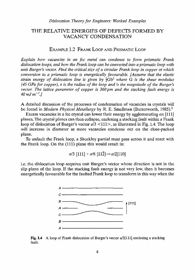
Excess vacancies in a fcc crystal can lower their energy by agglomerating on {111}planes. The crystal planes can then collapse, enclosing a stacking fault within a Frankloop of dislocation of Burger's vector a/3 <111>, as illustrated in Fig. 1.4. The loopwill increase in diameter as more vacancies condense out on the close-packedplane.
To unfault the Frank loop, a Shockley partial must pass across it and react withthe Frank loop. On the (111) plane this would result in:
a/3 [111] + a/6 [112] --+ a/2[110]
i.e. the dislocation loop acquires unit Burger's vector whose direction is not in theslip plane of the loop. If the stacking fault energy is not very low, then it becomesenergetically favourable for the faulted Frank loop to transform in this way when the
A-------------------------C-------------------------8---
A---
C----
8-------------------------A-------------------------
i[111]
Fig.l.4 A loop of Frank dislocation of Burger's vector a/3[111] enclosing a stackingfault.
4

Dislocations in Pure Materials
loop achieves a critical diameter such that the energy of the unfaulted loop(bounded by a dislocation of greater Burger's vector) is less than that of theoriginal.
Energy of the faulted Frank loop of radius r = 2'ITr(iGb2) + 'ITr 'YSF where 'YSF isthe stacking fault energy and b = a/3[111]. The energy of the unfaulted prismaticloop = 2'ITr(iGb2), where b = a/2[110]. Equating these energies and solving for r, wehave
i.e. r = [45.109 (!3602.10-24) - (i3602 .10-24)J/0.04 = 24.3 nm.
EXAMPLE1.3 FRANKLoop ANDTETRAHEDRALDEFECT
In gold the clustering of vacancies leads to a lattice defect of tetrahedral shape withstacking faults on its faces and stair-rod dislocations (al6<110» along each edge. Ifthe size of the defect tetrahedron is large, a triangular-shaped Frank sessile loop willhave a lower energy. Calculate the maximum size of the tetrahedron that can form, ifthe stacking fault energy of gold is 30 mJ m ", the lattice parameter is 408 pm and theshear modulus 42 GPa.
If the side of the tetrahedron is I, the area of each face 0.43312The total energy of the tetrahedral defect = 4 X 0.43312. 'YSF + 61.iGb2, where
b = a/6<110>The total energy of the triangular Frank loop = 31. !Gb2 + 0.43312. 'YSF
The maximum size of the tetrahedron can be found by equating these energies:
whence I = 42.109.4082.10-24/3.9.0.03 == 59.8 nm.
THE EFFECT OF POINT DEFECTS ON PLASTIC FLOW
It is recognised that the hardening produced by point defects introduced byquenching or irradiation is of two types:
(i) source hardening due to the pinning of dislocations by point defects in theform of coarsely spaced jogs;
(ii) a general lattice hardening which persists after initial yielding, which willchange the value of TO, the lattice friction stress (equation 1.5).
5

Dislocation Theory for Engineers: Worked Examples
Vacaflcy supersaturation stress
When an edge dislocation encounters a high supersaturation of vacancies, it will actas a vacancy sink and the dislocation will climb. The dislocation may be thought ofas being influenced by an effective stress somewhat analogous to osmotic pressure,known as the chemical stress.
EXAMPLE 1.4 CHEMICAL STRESS
Estimate the chemical stress which would be exerted on the dislocations in copper byeach of the following operations:
(a) quench from 1000°C to 150°C(b) 10% plastic strain at room temperature
The energy offormation of a vacancy may be taken as 1eV, and the Burger's vectorb = 0.25 nm.
The change in free energy dU when dn vacancies are added to the system attemperature T may be written:
dU/dn = Ef+ kTln(n/N)= -kTlnco+kTlnc= kTln(c/co)
where E, is the energy of formation of a vacancy, c the actual and Cothe equilibriumconcentration of vacancies at temperature T. This may be rewritten as
dU/dV = Energy/volume = stress, (J"c = (kT/b3) [In(c/co)] (1.2)
where dV is the volume associated with dn vacancies and b3 is the volume of onevacancy.
(a) Copper quenched from 1273 K to 423 K
The equilibrium concentration of vacancies at 1273 K will be given by
C2= exp[Ef/1273k]
At 423 K the equilibrium vacancy concentration is given by C1= [Ef/423k]. SinceIn(c2/c1) = (Ef/k)[423-1 -1273-1], from equation (1.2), the chemical stress «(J"c)acting at 423 K is therefore given by
(J"c = Eflb3 [1 - (423/1273)]
6

Dislocations in Pure Materials
Taking Ef = 1 eV (=1.6 X 10⁻¹⁹ J), and b = 0.25 nm we obtain:
(Tc = 6.84 GPa
(b) Plastically deformed copper
During cold work, vacancies are produced at dislocation jogs ansmg from theintersection of dislocations. The vacancy concentration c depends on the amount ofplastic strain 8 according to the approximate relation c = 10-48.
In the present case therefore c = 10-5•
At 300 K, Co = 1.69.10-17•
Substitution in equation (1.2) gives (Tc = 7.33 GPa.
THE EFFECT OF OTHER DISLOCATIONS ON PLASTIC FLOW
EXAMPLE 1.5 DISLOCATION DENSITY
Define the term 'dislocation density' and give typical values for Si, annealed Al andheavily cold worked Cu. Calculate the average dislocation spacing in a crystal with adislocation density of 1012 lines m:".
The density of dislocations in a crystal may be defined as the total length ofdislocation contained within unit volume (metres per cubic metre). For a randomarray of dislocations, an equivalent way of defining the density would be to expressit as the number of dislocations intersecting unit area, (m "),
In carefully prepared crystals of Si the dislocation density (p) ~ 106 - 108 m -2.
In annealed AI, p ~ 1010- 1012 m-2 and in cold worked Cu the density can rise to
1015- 1016 m".
Dislocation spacing. If p is the number of dislocations intersecting unit area, thenp1l2 is the number per unit length. Their spacing is therefore p -112, giving, forp = 1012 m -2, a spacing of 1 J.Lm.
EXAMPLE 1.6 AVERAGE PLASTIC SHEAR STRAIN
Express the average plastic shear strain (y), and the shear strain rate in terms of thenumber of mobile dislocations (N), the Burger's vector of the dislocations (b) and thearea of the slip plane that is swept when they move with an average velocity v.
7

Dislocation Theory for Engineers: Worked Examples
Consider a unit volume of crystal; it contains a slip plane of unit area. If a singledislocation sweeps over the slip plane, the displacement of the element will be b, sothe average shear strain will also be b.
If p dislocations sweep the plane, then the average shear strain is Nb. If (say) afraction A of the slip plane is swept, it follows that
'Y = ANb (1.3)
If the average dislocation velocity is v, it follows that the average shear strainrate = A Nbv.
Models of work hardening - simple 'forest' model
The dislocations in an undeformed crystal may be regarded as existing in theform of a network within each grain. Dislocations cannot end within a crystal:they either extend to the surface of the crystal, to a grain boundary or toother dislocations (forming a dislocation node). The shear stress required tocause a dislocation to glide on its slip plane will depend on the interactionthe gliding dislocation has with those other dislocations which intersect theslip plane and which might be regarded as 'trees in a forest'.
EXAMPLE 1.7 FOREST MODEL OF FLOW STRESS
On a simple 'forest' model, calculate the flow stress for dislocation glide in a crystalif the dislocation density is p.
A relationship may be derived in two ways:
1. Dimensional analysis
If the dislocations have Burger's vector b, an applied shear stress r will give rise toa force per unit length on a dislocation of magnitude ,.b (Peach-Koehler equation,Whelan, p. 51).1 The force of resistance to dislocation glide arises from interactionwith other dislocations and it may be written as exb2 (Whelan, p. 55),1 where ex is aconstant dependent upon the dislocation geometry. The balance of these forcesimplies that r (X b.
The flow stress will depend upon the shear modulus, G, the Burger's vector, b, andthe dislocation density p. The simplest dimensionless expression involving theseparameters may be written:
where C and m are constants.
8

Dislocations in Pure Materials
The requirement that T cc b indicates that m = !,giving the simplest expression forthe relationship between flow stress and dislocation density to be:
T = CGbpl!2
2. Simple cubic network
If it is assumed that the 'forest' dislocations of density p are arranged on a simplecubic network, then p1l2 is the number of dislocations per unit length, and p-1I2 istherefore the dislocation spacing. The applied shear stress causes the glidedislocation to bend to a radius of curvature R, where
Tb = TIR
Taking T as the line tension of the dislocation, T = !Gb2, this leads to the familiar
relationshipT = !GbIR (1.4)
If, at yield, we assume that the glide dislocation bows between the 'forest'dislocations, the maximum shear stress will correspond to the dislocation beingbowed into a semicircle of diameter equal to the forest dislocation spacing, i.e.
T = 2Gblp-1I2
If To is the lattice friction stress, then in general we can write the flow stress as:
T = TO + Gbo'" (1.5)where C is a constant.
EXAMPLE 1.8 A PARABOLIC STRESS-STRAIN RELATIONSHIP
Show that a parabolic stress-strain relationship is obtained if it is assumed that theflow stress is that necessary to move a dislocation in the stress field of thosedislocations surrounding it.
The first theory of work hardening, due to G. 1. Taylor, assumes that dislocationscreated during straining become stuck after travelling an average distance L. If themean distance between the dislocations is l, the stress necessary to move adislocation is given by
GbT=----
81T(1 - v) 1(1.6)
9
Dislocation Theory for Engineers: Worked Examplesr
" III
y
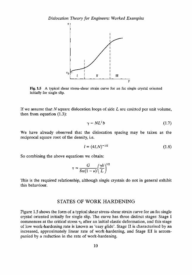
Fig.1.5 A typical shear stress-shear strain curve for an fcc single crystal orientedinitially for single slip.
If we assume that N square dislocation loops of side L are emitted per unit volume,then from equation (1.3):
(1.7)
We have already observed that the dislocation spacing may be taken as thereciprocal square root of the density, i.e.
l == (4LN)-1I2 (1.8)
So combining the above equations we obtain:
G (~b)1I2'T == 81T(1 - v) L
This is the required relationship, although single crystals do not in general exhibitthis behaviour.
STATES OF WORK HARDENING
Figure 1.5 shows the form of a typical shear stress-shear strain curve for an fcc singlecrystal oriented initially for single slip. The curve has three distinct stages: Stage Icommences at the critical stress 'To after an initial elastic deformation, and this stageof low work-hardening rate is known as 'easy glide'. Stage II is characterised by anincreased, approximately linear rate of work-hardening, and Stage III is accom-panied by a reduction in the rate of work-hardening.
10
Dislocations in Pure Materials
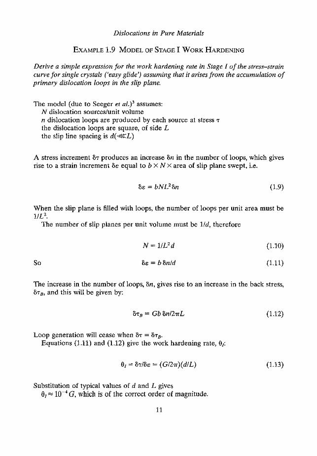
EXAMPLE 1.9 MODEL OF STAGE I WORK HARDENING
Derive a simple expression for the work hardening rate in Stage I of the stress-straincurve for single crystals ('easy glide') assuming that it arises from the accumulation ofprimary dislocation loops in the slip plane.
The model (due to Seeger et al.)3 assumes:N dislocation sources/unit volumen dislocation loops are produced by each source at stress l'
the dislocation loops are square, of side Lthe slip line spacing is d( ~L)
A stress increment 8,- produces an increase 8n in the number of loops, which givesrise to a strain increment 88 equal to b X N X area of slip plane swept, i.e.
(1.9)
When the slip plane is filled with loops, the number of loops per unit area must bel1L2.
The number of slip planes per unit volume must be l/d, therefore
(1.10)
So 88 = b 8n/d (1.11)
The increase in the number of loops, 8n, gives rise to an increase in the back stress,8,-B, and this will be given by:
(1.12)
Loop generation will cease when 81' = 81'B'
Equations (1.11) and (1.12) give the work hardening rate, 8/:
8/ = 8,-/88 = (G/27r)(d/L) (1.13)
Substitution of typical values of d and L gives81~ 10-4 G, which is of the correct order of magnitude.
11

Dislocation Theory for Engineers: Worked Examples
The behaviour of polycrystalline aggregates (The Taylor Factor)
A number of theories have been developed to predict the stress-strain curveof a polycrystalline aggregate from the behaviour of single crystals. Tayloradopted the von Mises criterion that five independent slip systems arerequired to cause a general shape change in a body, and in a given materialhe assumed that those five systems which operate in each grain are thosewhich require the least work. He equated the work done by the macroscopicstress (0") and strain (de) in the polycrystal to the work done by the five slipsystems in the individual grains. By a numerical treatment for a range ofcrystal orientations, he related the critical shear stress for slip (To) to 0" by:
m is known as the Taylor factor, and its value depend on the crystal structureof the material. An example of a calculation using this factor now follows.
EXAMPLE 1.10 NEUTRON IRRADIATION HARDENING
During neutron irradiation an assortment of dislocation loops are created in allmaterials by the Frenkel pairs which emanate from the primary knock-ons andsubsequent cascades produced by the incident neutrons. The increased dislocationloop density provides an additional set of barriers to glide dislocation movement andhence an increase in the yield strength of the material. This can be modelled usinganalogous arguments to those for Orowan strengthening (see section 3.2). Odette"has proposed the following equation for yield strength increase:
Where Iii is the Taylor factor, relating the shear stresses on a slip plane in a singlecrystal to the applied stress in a polycrystal, f is a random array efficiency factorassuming that the obstacles are perfectly hard, and is usually about 0.8, a is theobstacle strength (=1 in the case of precipitates), G is the shear modulus, b is theglide dislocation Burger's vector, n is the loop density and d is their averagediameter.
In this approach the inter-obstacle spacing in the Orowan equation (3.2) has beenreplaced by the term (nd)-1I2, which is equivalent to the inter-loop spacing. The a
12
Dislocations in Pure Materials
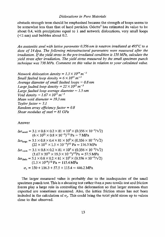
obstacle strength term should be emphasised because the strength of loops seems tobe somewhat less than that of hard particles. Odette" has estimated its value to beabout 0.4, with precipitates equal to 1 and network dislocations, very small loops«1 nm) and bubbles about 0.2.
An austenitic steel with lattice parameter 0.356 nm is neutron irradiated at 495°C to adose of 14 dpa. The following microstructural parameters were measured after theirradiation. If the yield stress in the pre-irradiated condition is 150 MPa, calculate theyield stress after irradiation. The yield stress measured by the small specimen punchtechnique was 738 MPa. Comment on this value in relation to your calculated value.
Network dislocation density = 1.3 X 10¹⁴ m ?
Small faulted loop density = 6 X 1O" m:'Average diameter of small faulted loops = 0.8 nmLarge faulted loop density = 22 X 1O" m-3Large faulted loop average diameter = 1.5 nmVoid density = 1.67 X 1~1 m-3Mean void diameter = 19.3 nmTaylor factor = 3.1Random array efficiency factor = 0.8Shear modulus of steel = 81 GPa
Answer
~O"small = 3.1 X 0.8 X 0.2 X 81 X 109 X (0.356 X 10-9/Y2)(6 X 1021 X 0.8 X 10-9)112 Pa = 7 MPa
dO"large = 3.1 X 0.8 X 0.4 X 81 X 109 X (0.356 X 10-9/Y2)(22 X 1021 X 1.5 X 10-9)112 Pa = 116.3 MPa
~O"voids = 3.1 X 0.8 X 0.2 X 81 X 109 X (0.356 X 10-9/Y2)(1.67 X 1021 X 19.3 X 10-9)1I2Pa = 57.5 MPa
~O"disln = 3.1 X 0.8 X 0.2 X 81 X 109 X (0.356 X 10-9/Y2)(1.3 X 1014)112 Pa = 115.4 MPa
O"y = 150 + 116.3 + 57.5 + 115.4 = 446.2 MPa
The larger measured value is probably due to the inadequacies of the smallspecimen punch test. This is a shearing test rather than a pure tensile test and frictionforces play a large role in controlling the deformation so that larger stresses thanexpected are sometimes measured. Also, the lattice friction stress has not beenincluded in the calculation of 0"y' This could bring the total yield stress up to valuesclose to that observed.
13

Dislocation Theory for Engineers: Worked Examples
DISLOCATION/GRAIN BOUNDARY INTERACTIONS - THEHALL-PETCH EQUATION
We will make two approaches to this process, the first considering the effect of thegeneral increase in dislocation density at yield, and the second assuming thesedislocations are in the form of a pile-up.
DISLOCATION FOREST ApPROACH
One simple derivation of the Hall-Petch relation starts from equation (1.5) - therelationship between the flow stress and the dislocation density. When a polycrystalof grain size d undergoes plastic yield, dislocations are assumed to be injected intothe grains by the grain boundaries, and the yield stress will be given by equation(1.5). If a length m of dislocations is produced per unit area of grain boundary atyield, then each grain will generate a total length of dislocation = m X 47'i(d/2)2. Thislength will, on average, be shared between two grains, so the dislocation densitygenerated at yield will be given by:
_ ~m4TI(~rp- 4TI(~r/3
= 3m/d
Substituting in equation (1.5), we obtain:
T = To + CGb(3m)1I2d-1I2
i.e. (1.14)
which is the Hall-Petch equation. The lattice friction stress, To, can be equated withthe Peierls stress of the material (jF
2G (-27'iW)«»= (l_v)exp -b-·
where v is Poisson's ratio and W is the dislocation width (it is usually assumedw = lOb).
14

Dislocations in Pure Materials
EXAMPLE 1.11 THE HALL-PETCH RELATIONSHIP (1)
The lower yield stress, ay, of annealed iron (grain size 16 grains mm=) is 100 MPa,and 250 MPa for a specimen with small grain size (4096 grains mm=). Determine thelower yield stress of iron with grain size 250 grains mm >.
Tensile stresses will be related to the grain size by a similar expression to equation(1.14), which refers to shear stresses, by introducing an orientation factor m relatingthe applied tensile stress 0" to the shear stress, T, i.e. 0" = tin,
Let us first express the grain size in terms of d:
grains mm""16
2504096
grains mm"4
15.864
d (mm)0.250.06320.0156
d-1I2O"y (MPa)100?250
23.988
Substitution in equation (1.14) in terms of the tensile stress gives:
250 = 0"0 + 8ky
100 = 0"0 + Zk;
:.150 = 6ky, so k; = 25 and 0"0 = 50
For a grain size of 250 mm ? we obtain O"y = 149.4 MPa which is the answerrequired.
DISLOCATION PILE-UP ApPROACH
The principle of grain boundary strengthening is outlined in Fig. 1.6. If the averagegrain size is d, a number n of dislocations pile-up at the grain boundary over adistance d/2 as a result of the applied resolved shear stress, Ts, operating a source ofdislocations at the grain centre, Sl.
Now the local stress at the head of the pile-up, acting on the lead dislocation, isn times the applied stress at the source. When this local stress exceeds a critical valueTc (the grain boundary shear strength), the blocked dislocations are able to glide pastthe grain boundary. Thus
Eshelby et al? have shown that
n = 'TrTs(d/2)/Gb (1.15)
15

Dislocation Theory for Engineers: Worked ExamplesGrain
boundary
Fig. 1.6 Dislocation model for the propagation of yielding past a grain boundary.
But 'Ts is equal to the applied stress (r) minus the lattice friction stress ("0).So by substituting for n and for "s, we can write
(1.16)
At yield, ,. = "y, so equation (1.16) can be rearranged to give:
_ (2GbTc)1I2d -112,. - "0+ --y 1T
which is the Hall-Petch equation (1.14) with
k; = (2Gb,. c/1T )112
EXAMPLE 1.12 THE HALL-PETeH RELATIONSHIP(2)
The following tensile data for the lower yield point for 70-30 brass were obtained at20°C. 64.7 MPa for a grain size of 100 uni and 188 MPa for a grain size of 6.25 J.Lm.Calculate the grain boundary shear strength Tc at 20°C given:Shear Modulus of brass = 48.3 GPaDislocation Burger's vector in brass = 0.255 nm
We will assume an orientation (Taylor) factor (m) of 3.1 for the fcc material, soequation (1.14) becomes:
16
Dislocations in Pure Materials
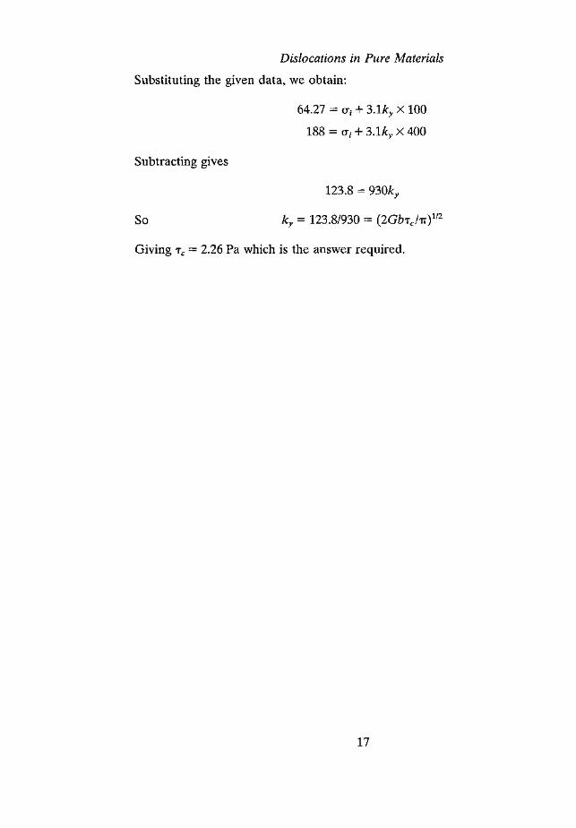
Substituting the given data, we obtain:
64.27 = c, + 3.1ky X 100
188 = a, + 3.1ky X 400
Subtracting gives
So
123.8 = 930ky
k; = 123.8/930 = (2GbTc/7r)1I2
Giving Tc = 2.26 Pa which is the answer required.
17

2Dislocation Interactions in Single
Phase Materials
The behaviour of dislocations in crystals containing solute elements may be affectedin two ways. If the solute atoms are able to diffuse in the lattice, the energy ofinteraction between the strain field of the dislocation and that of the solute atommay lead to the solute atoms segregating to the dislocations, leading to possiblelocking and yield point phenomena. Only a very small atomic fraction of solute isrequired to cause this effect which may raise the yield stress (i.e. the stress to initiateplastic flow in a previously undeformed crystal) but have little influence on the flowstress (the stress required to cause continuing plastic flow in a crystal).
In concentrated solid solutions, randomly dispersed solute atoms can act as pointobstacles to dislocation movement, and this can lead to a raising of the flow stressof the crystal. We will consider these two situations in turn.
SEGREGATION OF SOLUTE ATOMS TO DISLOCATIONS
EXAMPLE 2.1 THE MAXIMUM TEMPERATURE OF SEGREGATION
Assuming the atomic concentration of solute, c, around a dislocation line attemperature T can be described by the expression
c = Co exp(WlkT)
where Co is the atomic concentration of the solute in the dislocation-free crystal, k is theBoltzmann constant and W is the binding energy, estimate the temperature belowwhich yield points would be observed if the maximum binding energy is 0.5 eV andCo = 10-5•
Strong yielding behaviour is expected up to temperatures at which a condensedatmosphere of solute exists at the dislocation. This corresponds to a value of c of
19

Dislocation Theory for Engineers: Worked Examples
unity, we may therefore substitute in the equation:
i.e.
1 = 10-5 exp(0.5/8.62 X 10-5 X T)
T = 0.5 X 10⁵/(8.62 X 11.51) = 504K = 231°C.
This is the required temperature, below which yield points would be observed.
EXAMPLE 2.2 SOLUTE INTERACTION WITH AN EDGE DISLOCATION
An edge dislocation lies along the z direction and its Burger's vector b is parallel to x.The stress field of the dislocation is
0"xx = - Dy(3x2 + y2)/(X2 + y2)2O"yy = Dytx? + y2)/(X2 + y2)2
O"zz = v(<Txx + <Tyy)
<Txy = Dx(x2 - y2)/(X2 + y2)2O"xz = O"yZ = 0
where D = Gb/2'1T(1 - v), G is the shear modulus and v is Poisson's ratio. Derive anexpression for the pressure near the dislocation and sketch contour maps of itsdistribution. Explain the physical importance of the pressure in relation to solutionhardening.
y
y
x
(a) (b)
Fig 2.1(a) Showing an edge dislocation lying along the z direction, with its Burger'svector parallel to x. (b) Showing lines of equal pressure (full lines) and lines of flow(broken lines) for solute atoms migrating to an edge dislocation. The arrows denotethe direction of flow.
20

Dislocation Interactions in Single Phase Materials
The hydrostatic pressure, p, is defined by:
and this may be expressed in polar co-ordinates (Whelanl p. 30) as
p = 2(1 + v)D sin 8/3r
As shown in Fig. 2.1(a), r = 2R sin 8
.'. sin 81r = 1/2R
so the pressure is constant round a circle of radius R, and contours of constantpressure may be drawn as shown in Fig. 2.1(b).
Solution hardening
The interaction energy between a solute atom of misfit volume dv and thedislocation will be approximately p dv.
If the radius of the solute atom is r(l + s) instead of r, I1v = 30s (where 0 is theatomic volume)
The interaction energy (Eint) ::::::3p OsFor maximum interaction, R::::::b, and 8 = 90°:
2(1 + v)D sin 8p = 3r
= 2(1 + v)D3 X2b
Substituting for D, we obtain:
GOs(l + v)Einteraction = 21T(1 - v)
Substituting typical values for the parameters gives an interaction energy of theorder 0.1 eV This is therefore a relatively weak interaction.
EXAMPLE 2.3 THE RATE OF STRAIN AGEING
Assuming the interaction energy of a solute atom at a radial distance r from adislocation is proportional to r ", show that the increase in concentration of solute atthe dislocation core varies as (Dt/T)2/3 where D is the bulk diffusion coefficient of thesolute, T the temperature, and t the ageing time. How may this relation be testedexperimentally?
21

Dislocation Theory for Engineers: Worked Examples
In Fig. 2.1(b), the pressure contours are surfaces of constant interaction energy,hence the flow of solute atoms takes place down the pressure gradient, i.e. alonganother set of circles as indicated as dotted lines in the figure.
The small routes are exhausted first, then only the flow lines with larger radii arestill active. In the strain field of a dislocation, a solute atom is subjected to a forceF = - grad Einh controlling a drift velocity, v, given by the Einstein equation
v = DFlkT (2.1)
If Eint ex: 11r, we can put Eint = -Air, where A is a constant. The mean gradient of Eintalong a flow line of radius r is of the order dEin/dr, therefore F = Air.
In time t, all solute atoms within a radius r = ro will reach the dislocation, so, fromequation (2.1), the mean speed of a solute atom round the line is given by
dr/dt = DAlr kT
fro DArdr=-dt
o kT3DA
:.r5= kT t
The concentration, c, of solute at the dislocation will be given by
C = Co + ('ITY61b2) Co
= Co + co( 'ITlb2)(3DAtlkT)2/3 (2.2)
which is the required relationship.An internal friction method may be used to measure the fraction of carbon atoms
remaining (in random solution) in iron specimens after ageing them by variousamounts. It is found that this amount varies linearly with t2/3 as required inequation (2.2).
DISLOCATION DYNAMICS OF YIELDING
One of the reasons why iron containing carbon or nitrogen shows very marked yieldpoint effects is because there are strong interactions between these solute atoms andthe dislocations. The distortions caused by these atoms, which occupy the octahedralinterstices, are non-centrosymmetrical- having both a hydrostatic and shear nature- thus locking both screw as well as edge dislocations, so that the mobile dislocationdensity is very low.
22

Dislocation Interactions in Single Phase Materials
When such an alloy yields plastically the density of mobile dislocations issuddenly increased, and the yield point phenomenon can be explained byconsidering the dynamics of the dislocation motion.
The strain-rate 8 is given by
(2.3)
where 8e and 8p are the elastic and plastic strain rates respectively. We can write (seesection 1.6)
(2.4)
where Pm is the mobile dislocation density, b is the Burger's vector, and v thedislocation velocity. If pre-existing dislocations are firmly locked, plastic flow at theyield point may be controlled by the multiplication of new dislocations. The densityof mobile dislocations, Pm, may be expressed as
Pm =fp (2.5)
where f is a constant and P is the total dislocation density. p will be a function of theplastic strain, 8p' i.e.
P = Po + C8p (2.6)
where C is a constant, and Po is the dislocation density prior to straining.For a given value of Ep, if Pm increases, equation (2.4) indicates that v must
decrease. The dislocation velocity will depend upon the applied shear stress, and wemay write empirically:
(2.7)
where "0 and m are constants. If work hardening is taken into account, the effectivestress should be used in equation (2.7), i.e.
(2.8)
where e is the work-hardening rate.
EXAMPLE 2.4 UPPER AND LOWER YIELD POINTS
Derive an expression for the form of stress-strain curve of material which exhibits ayield point due to dislocation multiplication. What are the values of the upper yieldpoint and lower yield point, and upon what parameters does the magnitude of the yield
23

Dislocation Theory for Engineers: Worked Examplesr
Fig. 2.2 The form of equation (2.9).
drop depend?
We may substitute equations (2.5), (2.6) and (2.8) into (2.4) to obtain:
which can be re-arranged to give:
(2.9)
Initially, as a specimen is strained at a constant strain rate, B, most of the strainproduced is elastic, since Bp ~ Be, and the stress follows the elastic line (Fig. 2.2). Asa result of dislocation multiplication and the increase in stress, the contribution fromBp increases until the whole of the strain rate is due to plastic flow.
Further increase in strain leads to a decrease in stress, due to the decrease indislocation velocity (the second term in the above equation).
The upper yield point
The upper yield point thus corresponds to the stress at which 8p = 0, giving:
(
• ) 11m_ 8p'TllYP - 'To Pofb (2.10)
The stress decreases until the work-hardening term (i.e. the first term in the equationto the curve) becomes more important.
24

Dislocation Interactions in Single Phase Materials
The lower yield point
This is when dr/ds == O.We can rearrange equation (2.9):
_ (Bp ) 11m ( 1 ) 11m'T - as + 'To -
p fb Po + Ce.,(2.11)
So by differentiation and putting dr/ds = 0, a value of sp at the lower yield point('TlYp) is obtained. Substitution of this value into equation (2.9) will give 'Tlyp"
Thus yield points are produced which are more pronounced the smaller the valueof m. m is ----2 for Ge at high temperature, ----25 for LiF, "-'35 for Fe-Si alloys and----200 for fcc metals. Yield points are therefore not observed in pure fcc crystals,except in whiskers or dislocation-free crystals (Po = 0). The size of the yield drop willincrease with decreasing work-hardening rate (8) and increasing value of C, whichdescribes the multiplication rate of the mobile dislocations.
STRENGTHENING BY SUBSTITUTIONAL SOLUTE ATOMS
We have seen that dislocation pinning by solute atoms is normally associated withdilute solid solutions, but the solute atoms segregate preferentially to the disloca-tions. The yield stress is thus raised, but after yielding has occurred, the (solute-free)mobile dislocations will encounter few solute atoms (since the alloy is dilute), solittle increase in the flow stress over that for the pure metal is to be expected. Thisexplains the yield point phenomena observed, for example, in steels.
In order, therefore, to induce significant solute hardening, we would require amore concentrated solid solution and the increase in strength will arise from theinteraction between the glide dislocations and the individual solute atoms theyencounter upon the glide plane. Each solute atom may be regarded as a pointobstacle to the gliding dislocations, and a relationship may be derived between theyield stress of such an alloy and the force F exerted by each point obstacle upon thedislocations.
EXAMPLE2.5 THE CRSS FOR A CRYSTALCONTAININGA RANDOM ARRAYOFPOINT OBSTACLES
Show that if there are N, obstacles per unit area of slip plane, each of strength F, theflow stress T is given by
where G is the shear modulus and b the Burger's vector.
25

Dislocation Theory for Engineers: Worked ExamplesT T
Fig. 2.3 Showing a dislocation held up at an array of point obstacles.
We will be using the symbol 'T for shear stress and 'Tc for the CRSS, based on themodel illustrated in Fig. 2.3, which shows a dislocation interacting with the soluteatoms, which are treated as point obstacles of identical strength lying in the slipplane. The glide dislocation bows out between the particles as shown and, when theincluded angle <t>between the two arms of the dislocation reaches a certain criticalvalue, the dislocation breaks away from the obstacle. We shall refer to this value of<t>as the breaking angle, and at this critical point the obstacle strength, F, is relatedto the dislocation line tension, T, by
F == 2T cos!<t> (2.12)
When the breaking angle <t>== 0, the particle behaves as an impenetrable obstacle,while for values of <t>> 0, the obstacle can be sheared by the glide dislocation, withthe required shearing force equal to F.
The shear stress needed to cause the dislocation to break away from the obstaclemay be related to the obstacle strength F as follows. The applied shear stress, 7,
causes the dislocation of Burger's vector b to bow into an arc of radius of curvatureR, where
rrb == TIR (2.13)
From Fig. 2.3 it can be seen that
2R sin e == A
so
rrb == (2Tsin e)/A
But it can also be seen that e == 90° - !<t>,hence from (2.12) we have
vb == FIA
i.e. rrbA == F (2.14)
26

Dislocation Interactions in Single Phase MaterialsB'
,-,/,,,
/,-,-
;-,
Fig.2.4 The Friedel process for dislocations interacting with point obstacles.
It is important to determine how A, the effective obstacle spacing along thedislocation, depends upon the applied stress. Friedel approaches this by assumingthat during the yielding process the dislocation takes up a steady-state configuration,namely that each time a dislocation breaks through one obstacle (B, in Fig. 2.4) itmeets one, and only one, other obstacle (B' in Fig. 2.4) as it bows out to theconfiguration compatible with the stress applied (equation 2.13).
Each time an obstacle is sheared, an area A of the slip plane (shown shaded inFig. 2.4) is swept out by the dislocation. On average, the value of A is thus inverselyproportional to the number of obstacles per unit area of slip plane (Ns). Theso-called 'square lattice spacing', L, between the obstacles is given by
and
In Fig. 2.4 the area swept out per obstacle sheared will be given approximately -byto; so
L2 = hs: (2.15)
From the property of a circle (Fig. 2.4),
A2 = 2hR, for h -e; R (2.16)
Eliminating h from equation (2.15) and (2.16), we obtain
i.e. (AIL)2 = sec!<f>= 2TIF (2.17)
27

Dislocation Theory for Engineers: Worked Examples
The effective spacing of the obstacles, A, thus depends upon the value of thebreaking angle, <p, and hence upon F. Because the dislocation has some flexibility,the number of obstacles it touches per unit length increases as the obstacles becomestronger, hence the smaller the value of A. This decrease in A more than offsets theincrease in the 'square lattice' spacing of the obstacles.
Substituting for A in equation (2.14) we obtain a value for the yield stress,
(2.18)
Alternatively, this may be expressed in terms of the breaking angle through equation(2.12) as
To obtain the required expression, equation (2.18) may be squared and substitutionmade for T and for L. T is often taken as 4Gb2
, where G is the shear modulus, andL = N;1I2 giving
(2.19)
This is the required expression.Insofar as N, is proportional to the solute content of the alloy, equation (2.19)
indicates that the yield stress should be proportional to the square root of the solutecontent of the alloy. This relationship is not always observed in practice.
The magnitude of F is sensitive to atomic size differences between solvent andsolute, and also to differences in elastic properties. Fleischer" has defined a mismatchparameter, e, which combines both of these contributions. This leads to a definitionby Mott and Nabarro? such that
_ Gbe 2/3
'T - 2A' c (2.20)
where A' is the average dislocation line length. This contrasts with equation (2.19)which implies a c1l2 relationship with 'T since N, o: c. The experimental data availablemake it difficult to distinguish between these two relationships: often a simple linearrelationship is assumed.
EXAMPLE 2.6 SOLUTE HARDENING IN STEEL
Plain carbon steels are alloyed with so-called microalloying elements like Nb, W, Vand Ta. Much of the purpose of this is to provide precipitation strengthening.However, all of these elements contribute to solution strengthening. Assuming that 5atomic percent of each of these elements remain in solution in a steel intended for a
28

Dislocation Interactions in Single Phase Materials
railway line application, calculate the contribution to the yield strength of the steel for(a) Nb, (b) W, (c) Ta, and (d) V.
Data:
Atomic radii
ex-ferrite = 0.1241 nmNb = 0.142nmW = 0.1368nmTa = 0.143nmV = 0.131nm
Average dislocation line length = 50 nmShear modulus of iron = 8.1 X 10⁴ MPaBurger's vector = 2 X 10⁻¹⁰ m
Solution
Calculate the misfits for each element.
= 0.142 - 0.1241 = 0 144 Nbe 0.1241 .
= 0.1368 - 0.1241 = 0 124 We 0.1241 .
= 0.143 - 0.1241 = 0 154""-:e 0.1241 . ra
= 0.131 - 0.1241 = 0055 Ve 0.1241 .
Hence the yield stress contribution for solution strengthening is
8.1 X 1010 X 2 X 10-10 X (0.05)2/3X e'T = 2 X 5 X 10-8 Pa
This gives values as follows:
Nb 'T = 3.16 MPaW 'T = 2.7MPaTa 'T = 3.4 MPaV 'T = 1.2MPa
29

3Dislocation Interactions in
Two-Phase Alloys
.Particle hardening
The effect of dispersed precipitates upon the yield stress can be assessedby treating the microstructure once more as an array of point obstacles.When a shear stress is applied, the glide dislocations bow out between theparticles as shown in Fig. 2.3. When the breaking angle <p = 0, the particlebehaves as an impenetrable obstacle, while for value of <p > 0, the particlescan be sheared by the glide dislocations, with the required shearing forceequal to F. We will consider these two types of interaction separately.
PARTICLE SHEARING BY DISLOCATIONS (<p > 0)
Application of the point obstacle theory leads to an expression for the shear yieldstress given by:
(2.19)
Precipitate particles can impede the motion of dislocations through a variety ofinteraction mechanisms. Those for which theories for the value of F (or 4» have beendeveloped include:
(i) chemical strengthening, which arises from the energy required to create anadditional particle/matrix interface when the particle is sheared by thedislocation;
(ii) stacking-fault strengthening, which occurs when there is a difference betweenthe stacking-fault energy of the particle and that of the matrix when these areeither both fcc or hcp in structure;
31
Dislocation Theory for Engineers: Worked Examples
(iii) modulus hardening, which arises from differences between the elastic moduli ofthe matrix and particle;
(iv) coherency strengthening, which arises from the elastic coherency strainssurrounding a particle that does not fit the matrix exactly;
(v) order strengthening, which is due the additional work required to create anantiphase boundary in the case of dislocations passing through precipitateswhich have an ordered lattice.
We will, by the use of simple dislocation models, derive expressions for F inequation (2.19) for several different dislocation-particle interactions, and henceestimate of the yield stress for these situations.
EXAMPLE 3.1 CHEMICAL STRENGTHENING
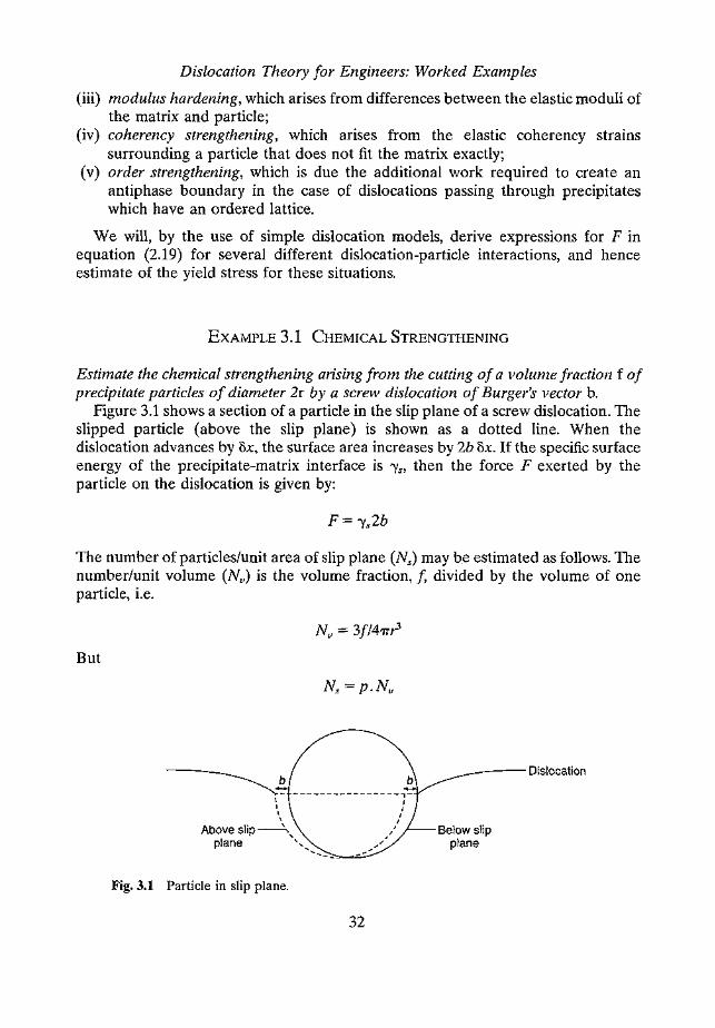
Estimate the chemical strengthening arising from the cutting of a volume fraction f ofprecipitate particles of diameter 2r by a screw dislocation of Burger's vector b.
Figure 3.1 shows a section of a particle in the slip plane of a screw dislocation. Theslipped particle (above the slip plane) is shown as a dotted line. When thedislocation advances by Sx, the surface area increases by 2b Sx. If the specific surfaceenergy of the precipitate-matrix interface is "Is, then the force F exerted by theparticle on the dislocation is given by:
The number of particles/unit area of slip plane (Ns) may be estimated as follows. Thenumber/unit volume (Nv) is the volume fraction, f, divided by the volume of oneparticle, i.e.
But
----',l: ----------------,~\ I\ I\ I\ I
Above slip~ / Below slipplane -. ",/ plane
••....•... ",""---- -
--- Dislocation
Fig. 3.1 Particle in slip plane.
32

Dislocation Interactions in Two-Phase Alloys
where p is the probability that a plane will intersect a single particle placed randomlywithin a unit cube. Since, of the various positions of the cross-sectional plane, onlythose positions existing over the length 2r would lead to the plane intersecting thesingle sphere, the probability of intersection is equal to 2r, so,
Giving
(3.1)
Substitution in equation (2.19) leads to:
1" = ( 12f )112!. ",3/2c 7TGb r IS
The theory thus predicts that, for a fixed volume fraction, f, the critical resolvedshear stress decreases as the particle size increases, contrary to what is normallyobserved in age-hardening. It therefore appears that chemical strengthening is notan important mechanism, except perhaps for particles of very small size.
EXAMPLE 3.2 STACKING-FAULT STRENGTHENING
Derive a simple expression for the shear yield stress of a crystal hardened by a volumefraction f of particles of diameter 2r, if there is a difference in stacking-fault energy~~SF between the lattice of the matrix and that of the particle (assume that the SFE ofthe particle is < that of the matrix).
If a dislocation in the matrix dissociates into two partial dislocations with anequilibrium separation Wm, when it moves into a particle of lower SFE it will splitfurther into a ribbon of width wp- This interaction will lead to a force being exertedby the dislocation on the particle, whose maximum value will be:
Where I is the length of dislocation inside the particle at the critical breakingcondition. I will be a function of the particle radius, say I = or, where ex is a constant'of the order 1.5.
Again equation (3.1),
Dislocation Theory for Engineers: Worked Examples
so substitution in equation (2.19) leads to:
= ( 3fr )112 (u Ll"lSF)3/2Tc 2'ITG b2
This model thus leads to a variation of the CRSS with Ll"l3J} and (f. r)1I2.Experimental data due to Gerold and Hartmann" on aged AI-Ag single crystalsshow good agreement with this model.
EXAMPLE 3.3 COHERENCY STRENGTHENING
Estimate the magnitude of F (and hence 'fe) arising from coherency strains associatedwith precipitates, if the shear strain in the matrix at a distance R from the precipitate(of radius r) is given by er'/R3
, where e is the misfit parameter of the coherentp recip itate.
The maximum strain and stress occur at the particle interface, i.e. at R = r, and wecan take the appropriate stress as approximately Ge. From the Peach-Koehlerequation, we can write the magnitude of the force per unit length experienced by adislocation of Burger's vector b as it approaches a particle as Geb.
This force acts effectively over a length of dislocation equal to the particlediameter, so we can write:
F:::::::2Gerbor
F:::::::kGerb
where k is a numerical constant which a more accurate treatment gives as between3 and 4. Substituting into equation (2.19), and replacing N, as before (equation 3.1),we obtain:
Tc = k3/2 Ge3/2(rlb )112(3/2'IT )112t'"The increment of CRSS due to the presence of the particles is thus predicted to beproportional to t'" and also to r1l2. Experimental data indicate that theseproportionalities are observed in practice, although the above expression over-estimates the actual values of Tc. It should be noted that the (rib) and f terms areboth related to composition, c. The above equation can therefore be used todemonstrate a c1l2 dependence on Te.
EXAMPLE 3.4 ORDER HARDENING
Estimate the maximum value of F (and hence 'fe) arising [rom the [ormation ofan antiphase boundary (apb) of energy 'Yapb in an ordered spherical particle ofradius r.
34

Dislocation Interactions in Two-Phase Alloys
The passage of a dislocation creates an apb in the particle, and an estimate of themaximum force exerted by a spherical particle may be obtained by assuming that thedislocation lies along a diameter, in which case
F = 2rYapb
Making the same substitutions as in the previous examples we obtain:
= (12 fr )112~~~2b'Tc 'ITO b2
This equation accounts for the increase in 'Tc in ageing in terms of the increase in rfor a given volume fraction. Order hardening is a very important hardeningmechanism in nickel alloys in which large volume fractions of the ordered ~'-phase(Ni3AI, Ni3Ti, or Ni3(AI, Ti)) may be present. A complication which commonly arisesin this class of alloy is that the dislocations travel in pairs - the first dislocationcreates an apb and the second restores the order. The approximation in the Friedelstatistics that the volume fraction of precipitates is small is not applicable to manynickel-based superalloys, where the volume fraction of v' precipitates can exceed 0.7in some alloys.
The strengthening behaviour of cubic ~' precipitates in such alloys is not modelledwell by the above or similar equations, where there is evidence that the yield stressdecreases with increasing precipitate sizes.
PARTICLE BY-PASS BY DISLOCATIONS - OROWANHARDENING (<p = 0)
As the magnitude of F increases, the breaking angle <p decreases, and eventuallybecomes zero. For larger values of F the dislocation bypasses the particle rather thanshears it.
EXAMPLE 3.5 EFFECT OF PARTICLE SPACING ON YIELD STRESS
Illustrate graphically the variation in the tensile yield stress (O"y) with particle spacing(L) for the case of particle by-pass by dislocations, in the case of aluminium.
[Lattice parameter 0.404 nm, shear modulus 26.2 GPa.j
When dislocation by-pass takes place, the force exerted by the particle is balancedby the line tension of the two arms of the dislocation on each side of the particle.Therefore F = 2T = Gb2
, and substitution in equation (2.19) leads to:
(3.2)
35

Dislocation Theory for Engineers: Worked Examples500~----------------------------------
50 100 300 700 1000 2000
m 400r------+----------------------------a,~~ 300r-------~~------------------------en~W 200r-----------~----------------------"0Q)
~ 100r---------------~------------------
Particle spacing - nm
Fig. 3.2 Orowan plot.
where L is the square lattice spacing of the particles (assuming that the particlediameter is negligible in comparison with L).
For the case of glide dislocations in aluminium, b = alV2 = 0.29 nm, giving:
r, = 26.2 X 109 X 0.29 X 10-91L = 7.61L (Pa)
Let us calculate Tc for a series of values of L:
L (nrn) 50 100 300 700 1000 2000
'Tc (MPa) 152 76 25.3 10.9 7.6 3.8
<Ty (MPa) 456 228 75.9 32.7 22.8 11.4
The tensile yield stress may be obtained from Tc by multiplying by the appropriateTaylor factor, which we will take as 3, for the case of an fcc crystal structure. Thethird row in the table is thus obtained and the data shown graphically in Fig. 3.2.
The yield stress of pure aluminium is about 3 MPa, and it is apparent from thegraph that significant Orowan hardening is only achieved when sub-microninter-particle spacings are present.
EXAMPLE 3.6 CALCULATION OF CRITICAL INTERPARTICLE SPACING
Discuss the effect of particle spacing on the type of dislocation-particle interaction.Calculate the precipitate spacing (L) necessary to give maximum hardening forprecipitates with a misfit (B) of 0.2 and with a volume fraction (f) of 0.02 in copper(lattice parameter 0.354 nm, shear modulus 45 GPa).
36

Dislocation Interactions in Two-Phase Alloys
Mott and Nabarro ' realised that the obstacles become impenetrable when the backstress arising from the energy contained within the particle becomes larger thanthe applied stress, 'T. The energy generated per unit volume by the particles isgiven by
E= Gef
This stress is equivalent to an energy per unit volume and is equal to the appliedstress needed to cause particle cutting rather than Orowan looping. Thus
'T = Gef= aGb/R
where R is the radius of curvature of the dislocation.Therefore
R = aGblGsf = able]
Remembering that the looping stress is at a maximum when R = A/2 and thata = 0.5, we obtain that the critical spacing, ACrit' for the maximum applied stress Gustbefore the back stress is insufficient to resist the applied stress, and thusparticle-cutting starts to take place) is:
Acrit = 2bl2sf = blsf
Substituting the values given, with b = atV2, we find:
Acrit = (0.354/1.414 X 4) 10-6 m = 63 nm,
which is the required answer.Nate that 'T c will decrease with particle size and spacing for spacings below ACrit.
This corresponds to the situation that <f> > 0 and is described in Section 3.3.
COMBINATION OF STRENGTHENING PROCESSES
EXAMPLE3.7 COMBININGGRAIN-SIZE, SOLUTEANDPARTICLESTRENGTHENING
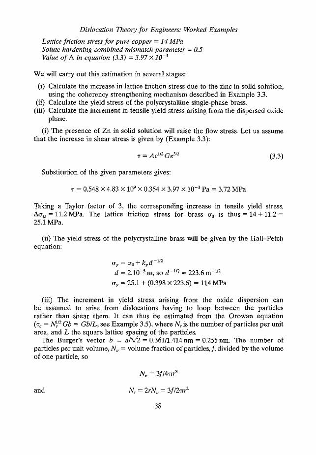
A specimen of a-brass (Cu-30 at.% Zn) contains a volume fraction of 0.028 ofspherical oxide particles of diameter 0.1 urn. The grain size is 20 urn. Estimate thetensile yield stress given the following data:
Shear modulus of brass = 48.3 GPaLattice parameter, a = 0.361 nmSlope of Hall-Petch plot, k, = 0.398 MPa m'"
37
Dislocation Theory for Engineers: Worked Examples
Lattice friction stress for pure copper = 14MPaSolute hardening combined mismatch parameter = 0.5Value of A in equation (3.3) = 3.97 X 10⁻³
We will carry out this estimation in several stages:
(i) Calculate the increase in lattice friction stress due to the zinc in solid solution,using the coherency strengthening mechanism described in Example 3.3.
(ii) Calculate the yield stress of the polycrystalline single-phase brass.(iii) Calculate the increment in tensile yield stress arising from the dispersed oxide
phase.
(i) The presence of Zn in solid solution will raise the flow stress. Let us assumethat the increase in shear stress is given by (Example 3.3):
(3.3)
Substitution of the given parameters gives:
T = 0.548 X 4.83 X 109 X 0.354 X 3.97 X 10-3 Pa = 3.72 MPa
Taking a Taylor factor of 3, the corresponding increase in tensile yield stress,~O"ss = 11.2 MPa. The lattice friction stress for brass 0"0 is thus = 14 + 11.2 =25.1 MPa.
(ii) The yield stress of the polycrystalline brass will be given by the Hall-Petchequation:
0" = 0" + k d -112Y 0 Y
d = 2.10-5 m, so d -1/2 = 223.6 m -1/2
O"y = 25.1 + (0.398 X 223.6) = 114 MPa
(iii) The increment in yield stress arising from the oxide dispersion canbe assumed to arise from dislocations having to loop between the particlesrather than shear them. It can thus be estimated from the Orowan equation(Tc = N~/2Gb = Gb/L, see Example 3.5), where N, is the number of particles per unitarea, and L the square lattice spacing of the particles.
The Burger's vector b = atV2 = 0.361/1.414 nm = 0.255 nm. The number ofparticles per unit volume, N; = volume fraction of particles, f, divided by the volumeof one particle, so
and
38

Dislocation Interactions in Two-Phase Alloys200~----------------~
Dispersion strengthening
150 increment (Orowan)
coo,~Cf)Cf) 100~Ui"0Q)
~ Grain sizestrengthening
50 (Hall-Petch)
Solid solution strengthening by ZnFriction stress of pure copper
00 100 200 300 400 500d-1f2(m-1f2)
Fig.3.3 The grain-size dependence of the yield stress in a dispersion-strengthenedCu-Zn alloy.
Substituting the given values of particle size and volume fraction givesN, = 5.35 X 10¹² m-2•
This corresponds to a square lattice spacing of particles, 0.432 urn.The increase in shear stress = Gb/ L
= 28.5 MPa.Again assuming a Taylor factor of 3, this predicts an increase in tensile yield stress
~86MPa.
Assuming that the total yield stress may be obtained by the linear addition ofthe Orowan contribution to the Hall-Petch increment, we estimate the yield stressto be:
O"y = 114 + 86 = 200 MPa
The individual contributions to this stress are indicated in Fig. 3.3.
39


4Effects at Elevated Temperatures
RECOVERY AND RECRYSTALLISATION
SUBGRAIN GROWTH DURING RECOVERY
Energy of symmetrical tilt boundary (misorientation 0)
This is treated as an array of parallel edge dislocations, all sharing the same Burger'svector, b. If D is the dislocation spacing, then as illustrated in Fig. 4.1:
sin(S/2) = b/2D
for small S we have:
e = biD
In unit area the dislocations are of unit length, and the number per unitarea = 1/D = S/b. The energy per unit area of the boundary is simply the sum of the
x
Fig.4.1 A symmetrical tilt boundary in a simple cubic lattice.
41

Dislocation Theory for Engineers: Worked Examples
energies of the individual edge dislocations (Ed)' where:
where E; is the core energy per unit length of dislocation line, and ro the inner cut-offradius from the dislocation. Therefore the boundary energy is:
(4.1)
where A and B are constants:
Gb GbA = Efb + 411"(1 _ v) In(bI2ro); B = 411"(1 - v)
Equation (4.1) is the Read-Shockley formula and its functional form applies to allsmall angle boundaries, not just symmetrical tilt boundaries.
EXAMPLE 4.1 DRIVING FORCE FOR SUBGRAIN GROWTH
Calculate the reduction in energy (.dE) resulting from the coalescence at a 'Y' junctionof two small-angle boundaries of misorientations eJ and e2 into a single small-angleboundary of misorientation (el + (2) as illustrated in Fig. 4.2.
81..l ..l
1- ..l
..l 1-
1- ..l
1-..l1-1-..l
81 + 82
Fig.4.2 A 'Y' junction between three tilt boundaries of misorientations OI, O2, and01 + 020
42

and
Effects at Elevated Temperatures
Egb1 = 81[A - B In 8dEgb2 = 82[A - B In 82]
E1+2 = (81 + (2) [A - B In(81 + (2)]
~E = Egb1 + Egb2 - E1+2
This is the driving force for sub grain growth during recovery annealling.
RECRYSTALLISATION
Stored energy of deformation
Heavily cold-worked metals recrystallise when annealed, the process beingdriven by the stored energy of deformation. The principal source of thisenergy lies in the form of dislocations, and calorimetric measurements duringa recrystallisation anneal provides a means of estimating the density ofdislocations in the cold-worked metal.
EXAMPLE 4.2 ENERGY RELEASED DURING RECRYSTALLISATION
The energy released when a cold-worked copper specimen is recrystallised is 1Mlm-3•
Taking the modulus as 48 GPa and a lattice parameter of 0.36 nm, estimate thedislocation density in the cold-worked state.
For a dislocation density p the stored energy is
E = pEdis
where Edis is the energy per unit length of dislocation line.Edis may be written:
e.; = Gb2f(v) In(R)
4'lT ro
43

Dislocation Theory for Engineers: Worked Examples
where R is the upper cut-off radius (usually taken to be the separation ofdislocations (p -112).
ro is the inner cut-off radius (usually taken as between band 5b)f( v) is a function of Poisson's ratio (v), which, for an average population of edge and
screw dislocations is ---(1 - v/2)/(1 - v).
The energy of a dislocation depends on its environment - being highest in a pile-upand lowest when in a cell or subgrain wall. In the present case, only a veryapproximate energy is needed, so the above equation can be simplified to
where c is a constant of the order 0.5.So we may write:
Ep = 0.5Gb2
In the present case, b = atV2 = 0.255 nm
p = 0.5 x 48 X 109 X 0.065 X 10-18
i.e. p = 6.4 X 10¹⁴ m-2
The driving pressure for recrystallisation
During the recrystallisation of cold-worked metals, therefore, the pressureacting on a migrating grain boundary arises from the line tension of thedislocations being annihilated. We have seen in Example 4.2 that thiscorresponds to an energy per m3 of 1 MJ, and so a pressure of 1 MPa willbe exerted per m2 of grain boundary, which can thus be regarded as thedriving force for primary recrystallisation.
44

Effects at Elevated Temperatures
DISLOCATION CLIMB - CLIMB RATE CALCULATION
EXAMPLE 4.3 MEASUREMENT OF STACKING- FAULT ENERGY FROM THE RATE
OF ANNIHILATION OF DISLOCATION Loops
A prismatic edge dislocation loop of vacancy character in an fcc metal is located nearthe centre of an equiaxed grain with grain size much larger than the loop diameter.Estimate the time taken for the loop to anneal out at 200°C if the initial radius of theloop is 50 nm. How would the annealing time differ if the loop were a Frank loop on{J11} enclosing an intrinsic stacking fault?
[Assume shear modulus = 25 GPa, Burger's vector of the prismatic disloca-tion = 290 pm, stacking fault energy 200 ml m:', self-diffusion coefficient at200°C = 3.5 X 10⁻²⁰ m2 S-l.j
When an edge dislocation encounters a high supersaturation of vacancies, it will actas a vacancy sink and the dislocation will climb. The dislocation may be thought ofas being influenced by an effective stress somewhat analogous to osmotic pressure.The magnitude of this chemical stress can be derived from Example 2.1 asrr = (kT/b3)[ln(c/co)]. The force per unit length on the dislocation, F, will be given byob, i.e.
F = (kT/b2)[ln(c/co)] (4.2)
which may be rearranged to express the concentration c of vacancies in the vicinityof an edge dislocation which is SUbjected to a force F per unit length:
c = Co exp(Fb2/kT)
But from the exponential series we may write for small x: e' ~ (1 + x).Therefore
(4.3)
Turning now to a consideration of the shrinking dislocation loop of radius r in aspherical crystal of radius R2(R ~ r), the problem is one of spherically symmetricaldiffusion. The dislocation experiences a force per unit length due to its curvature,giving rise to a local increase in vacancy concentration. (Fig. 4.3).
45
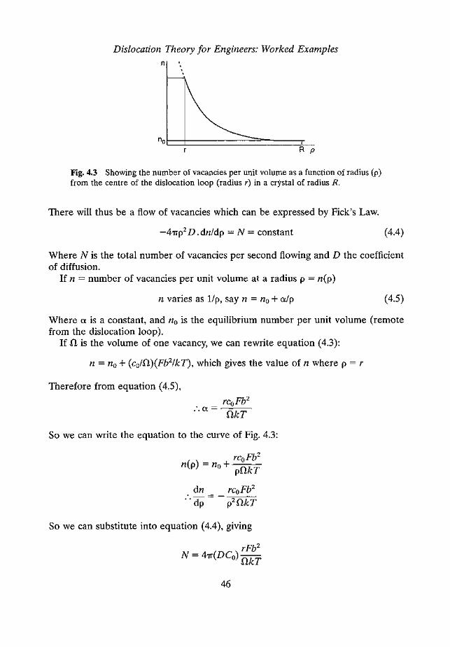
Dislocation Theory for Engineers: Worked Examplesn
Fig. 4.3 Showing the number of vacancies per unit volume as a function of radius (p)from the centre of the dislocation loop (radius r) in a crystal of radius R.
There will thus be a flow of vacancies which can be expressed by Fick's Law.
-41Tp2D .dnldp = N = constant (4.4)
Where N is the total number of vacancies per second flowing and D the coefficientof diffusion.
If n = number of vacancies per unit volume at a radius p = n(p)
n varies as lip, say n = no + (X/p (4.5)
Where (X is a constant, and no is the equilibrium number per unit volume (remotefrom the dislocation loop).
If n is the volume of one vacancy, we can rewrite equation (4.3):
n = no + (co/fl)(Fb2IkT), which gives the value of n where p = r
Therefore from equation (4.5),rcoFb2
:. (X = OkT
So we can write the equation to the curve of Fig. 4.3:
rcoFb2
n(p) = no + pflkT
So we can substitute into equation (4.4), giving
46

Effects at Elevated Temperatures
But DCo = Dsd, the coefficient of self-diffusion, since a given vacancy jumps Nlntimes as often as a given atom.
If .(27fr/b) vacancies arrive at the loop, its radius will shrink by b, so
dr b2 N 2Fb4 ti;- dt = 27fr = f!kT (4.6)
The force per unit length exerted on the dislocation arising from its line tension, I',when the dislocation is in the form of a loop of radius r, is given by fir. TakingF = !Gb2, and assuming the atomic volume n = b3, equation (4.6) becomes
dr Gb3Dsd
- r dt = kT
The time taken for the loop to shrink may thus be obtained by integrating thisequation, giving
[r]r = _ Gb3 Dsd [ ]02 kT t t
o
= 375 seconds, which is the required answer.
If the dislocation was in the form of a Frank loop, it would shrink more rapidly,because the stacking fault of energy 0.2 J m-2 provides an extra (constant) force perunit length of magnitude 0.2 Nm-1 (independent of the radius of curvature). If thisis substituted into equation (4.6) we find:
-drldt = (2Fb .Dsd)/kT
0.4 X 290 X 10-12 X 3.5 X 10-20
1.38 X 10-23 X 473
= 0.623 X 10⁻⁹ m S-1
So t = r10.623 X 10-9 = 5010.623 = 80 seconds.This indicates a four-fold reduction in the shrinkage time of the loop when it
contains a stacking-fault.
DISLOCATION CREEP
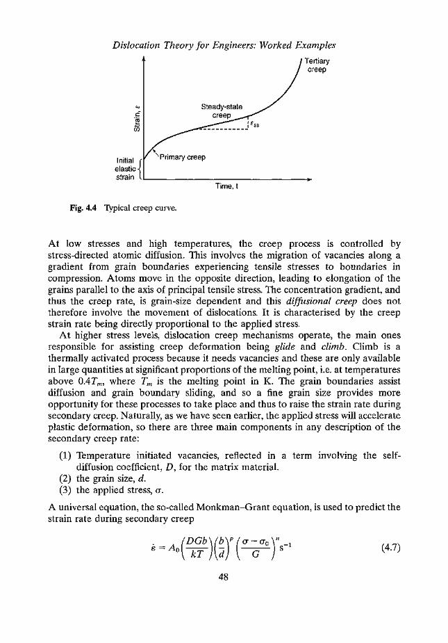
The significant' engineering parameter during high temperature deformation ofpolycrystals is the secondary (steady state) creep rate, which is the slope of the curveduring secondary creep, indicated in Fig. 4.4.
47
Dislocation Theory for Engineers: Worked ExamplesTertiarycreep
Initial {elasticstrain L-- ~
\ Primary creep
Time, t
Fig. 4.4 Typical creep curve.
At low stresses and high temperatures, the creep process is controlled bystress-directed atomic diffusion. This involves the migration of vacancies along agradient from grain boundaries experiencing tensile stresses to boundaries incompression. Atoms move in the opposite direction, leading to elongation of thegrains parallel to the axis of principal tensile stress. The concentration gradient, andthus the creep rate, is grain-size dependent and this diffusional creep does nottherefore involve the movement of dislocations. It is characterised by the creepstrain rate being directly proportional to the applied stress.
At higher stress levels, dislocation creep mechanisms operate, the main onesresponsible for assisting creep deformation being glide and climb, Climb is athermally activated process because it needs vacancies and these are only availablein large quantities at significant proportions of the melting point, i.e. at temperaturesabove 0.4Tm» where Tm is the melting point in K. The grain boundaries assistdiffusion and grain boundary sliding, and so a fine grain size provides moreopportunity for these processes to take place and thus to raise the strain rate duringsecondary creep. Naturally, as we have seen earlier, the applied stress will accelerateplastic deformation, so there are three main components in any description of thesecondary creep rate:
(1) Temperature initiated vacancies, reflected in a term involving the self-diffusion coefficient, D, for the matrix material.
(2) the grain size, d.(3) the applied stress, a.
A universal equation, the so-called Monkman-Grant equation, is used to predict thestrain rate during secondary creep
(4.7)
48

Effects at Elevated Temperatures
where Ao is a constant - 1010
D is the self-diffusion coefficientb is the Burger's vectork is Boltzmann's constantT is the absolute temperatured is the grain sizea is the applied stressao is the back -stress caused by already-existing dislocation obstaclesG is the shear modulus.
The parameters nand p refer to the creep mechanisms in operation, which dependon the stress and the temperature as already observed. For grain boundarydominated, or Coble creep, D is the grain boundary diffusion coefficient, p is 3 andn is unity. For lattice diffusion assisted, or Nabarro-Herring creep, D is the latticediffusion coefficient,. p is 2 and n is again unity.
At higher stresses, D is the lattice diffusion coefficient, p is zero, and n usually liesbetween 3 and 8. This regime of creep is known as power law creep. The regimes ofstress and temperature where these mechanisms operate are material-dependent,and maps defining them for different materials are to be found in Frost andAshby,"
Nomograph methods are also available for predicting creep failure (see Fig. 4.5).A number of sophisticated models have been developed to describe thephenomenon, but we will indicate how a simple power law creep relationship maybe derived from first principles.
EXAMPLE 4.4 RECOVERY CREEP MODEL
Assuming steady-state creep (deldi) to arise from a balance between the recovery rate(-da/dt) and the hardening rate (dolde), derive an expression for the stress andtemperature dependence of the creep rate.
We assume that the dislocations exist as three-dimensional network of average linklength I. Recovery processes will cause this network to coarsen. The applied stresswill cause the links in the network to bow out and act as dislocation sources. Workhardening during dislocation multiplication refines the network size, so that in asteady state the hardening and recovery processes balance to give a constantdislocation density, p, and a constant creep rate.
Considering first the hardening rate, h:The magnitude of the applied stress will determine the average value of I, and hence
the dislocation density, p:
49

Dislocation Theory for Engineers: Worked Examples
We can therefore write:
h = drr/ds ex: 1/e1l2 ex: 1/cr
Now consider the recovery rate, r:The rate of growth of the network, dlldt = mobility (M) X force, i.e.
dUdt = M X Til
where T is the line tension of the dislocation, i.e.
l dl = M. T dt; so l2 ex: t; i.e. p -1 ex: t; and cr-2 ex: t, i.e. rr ex: t-1I2
We can now write
Using these expressions for rand h we obtain
Steady state creep rate, i; = rlh ex: cr4
The dislocation mobility, M, will depend on the climb rates. The temperaturedependence of M and therefore e will be characterised at high temperatures by anactivation energy equal to that for lattice self diffusion (QSD), so that we obtain:
e = Acr4 exp( - QSDIRT)
where A is a constant.This power-law creep relationship is seldom obeyed in practice, and it is usually
expressed in the general form:
(4.7)
where the values of the constants A, nand Q vary from material to material andhave to be found experimentally.
EXAMPLE 4.5 POWER-LAW CREEP CALCULATION
A nickel alloy creeps in steady state according to the relation (4.7) above. The alloyis used to make a tensile strut inside a furnace. The strut is in the form of a rod 2 mmin diameter, and supports a load of 20 kg. Each day the furnace is run at 800°C for14 h and 850°C for 10 h. How long will it be before the strut breaks? [For this alloy,
50

Effects at Elevated Temperatures
n = 4.6, Q = 270 kJ mot:', A = 8.5 X 10⁻⁴ with a in MPa. Strain to rupture at 800°Cis 8% and is 12% at 850°C.]
The stress in the strut, (J" = 20 X 9.81hr MPa = 62.45 MPaNeglecting any tertiary creep, the time to fracture by creep tf will be given by:
where sf is the strain to fracture at temperature T.At 800°C:
tf = 0.08/ 8.5 x 10-4 X 62.454.6 exp( -270000/8.31 X 1073)= 7.31 X 10⁶ s= 2030.6 h
tf = 0.12/8.5 X 10-4 X 62.454.6 exp( -270000/8.31 X 1123)= 2.84 X 10⁶s= 788.9 h
Each day in service, the strut spends a fractional life of 14/2027.6 at 800°C and10/788.9 at 850°C. If n is the total lifetime in days, and assuming that the durationof tertiary creep is negligible and that the mechanism of creep failure is identical inthe two situations, we may write:
n[(14/2030.6) + (10/788.9)] = 1
whence n = 51 days.
EXAMPLE 4.6 USE OF THE MONKMAN-GRANT EQUATION (4.7)
Superheater tubes in a power station boiler are made from Type 316 stainless steel witha 100 J.Lmgrain size and operate at 550°C at a maximum stress of 50 MPa.
Calculate the design lifetime of the superheater assuming that accumulated strainsof less than 1% are specified. Compare your predictions with the empirical predictionsfor the same alloy using the Larson-Miller plot provided (Fig. 4.5).
51

Dislocation Theory for Engineers: Worked Examples
5
Larson-Miller parameter, T (20 + log t) = 10-3; T in oK, t in hours10 15 20 25 30
1002003004005006007008009001000110012001300140015001600170018001900200021002200
C')c,enc0~
10908070605040301"-. .••.. 25r-,20r-
\ 15
\ 10\. 9
°C, 8
1\ 720~ \ 6
100~ 1\ 5
~, 4
~ \ 3200
~~-
~~~~~~ 1\ 2300
~~~~~~ 1.5
400 ~~~~ 1~~~~~~~
500 ~~~~~~~~~~~~'"
600 ~~~~~~~~~~~~~~
700 ~~~~~~'"-, -, -, -,-.~"",
800 ~~~~~~~~~~~~
900 ~~~~~~'"-, -, -, -, -. -. -.1000 ~~~~~~~
~~~~~~~1100
""'~~""~~'"~~~~~~"",
1200 10-1 100'101 "'102"103 "104
Failure times at 1% strainTime - hours
52
35
o
C')c,
(\J:9 E0 E0
~ Ol~300 200
200 150
150 1009080100 7090 608070 5060 405040 30
30 220
20 15
15 109810 79 687 56 454 3
3 2
2 1.5
1.5 1

Effects at Elevated Temperatures
Data:In the Monkman-Grant equation:
Ao = 1010
G = 80GPab = 2.58 X 10⁻¹⁰ mp=On=5
lattice friction stress = 45 MPa
Pre-exponential constant in the diffusion equation = 10-4 rrr' S-l
Activation energy for self-diffusion = 240 kJ mor '
. _ -4 (_ 240 X 103) _ X -20 2-1.. D - 10 exp 8.31 X 823 - 5.7 10 m s .
Under power law creep, equation (4.7) becomes:
. _ A (DGb) (a - ao)5 -1E- 0-- --- skT G
.. = 10 (5.7 X 10-20 X 8 X 1010 X 2.58 X 10-10) ( 5 X 10⁶
)5
•• E 10 1.38 X 10-23 X 823 8 X 10¹⁰
i.e.
If the maximum strain is 10/0, then the time to reach this strain, t, is given by
8 0.01t = 8 = 9.9 X 10⁻¹⁰ s
i.e. t = 2811 hours.The stress is 50 MPa (5 kg mm "), reading this from the Larson-Miller plot (Fig.
4.5) gives a lifetime of around 1000 hours, which is adequate confirmation that themechanism-based calculation complies well with the empirical data.
53


5Dislocations in Fracture Processes
DUCTILE FRACTURE
Ductile fracture occurs by a linking of small voids set up around second phaseparticles in the alloy, as shown in Fig. 5.1. Assuming that the void linkage processdoes not contribute significantly to the failure strain (which will be the case whenthe spacing of the second phase particles is small), the critical step in the ductilefracture process is the opening of a void around the particle. Ashby'? has analysedthis problem and the mechanism turns out to be the accumulation of dislocation loopson secondary slip planes intersecting the particles. Enough dislocation loops at theinterface eventually introduce sufficient half-planes or stress that a void is openedup beneath the slip plane. It is useful in the design of particle-strengthened systemsto identify the ideal requirements of the particle size distribution for the maximumresistance to ductile failure, and the Ashby analysis enables us to do this.
APPliej stress
Voids
IHParticles
1Fig. 5.1 Ductile fracture.
55

Dislocation Theory for Engineers: Worked Examples
Shear
Tensile/aXiS/
/
PrimaryCavity
Fig. 5.2 Showing how tensile stress in the particle-matrix interface leads to theopening up of a cavity.'
EXAMPLE 5.1 CALCULATION OF DUCTILE FRACTURE STRAIN IN A STEEL
Calculate the fracture strain for a steel with a volume fraction of 1% carbides with amean radius of 10 nm. The properties of the steel are as follows:Carbide-matrix interfacial energy = 0.6 J m ?
Poisson's ratio = 0.28Shear modulus = 81 GPa
The required equation is derived by assuming that self-interstitial loopsaccumulating on secondary slip systems during plastic deformation will exert a stresson the particle-matrix interface (see Fig. 5.2). The loop closest to the interfacecarries the majority of the stress to the interface, and its distance from the interfaceis the length of the loop stack divided by the number of loops in the stack. This stressvaries as the reciprocal of the distance from the loop to the particle-matrix interface.The stress at the interface is thus proportional to the number of loops in the stackdivided by the length of the dislocation loop stack. Unless the particle spacing is verylarge, the loop stack size can be approximated to the interparticle spacing, 'A. Thenumber of loops in the stack is related to the Burger's vector b, the particle diameterderit, and the strain at the interface, e. Hence the interface stress, UTerit required togenerate the fracture strain eF is given by:
e derilITT = a--
crit 'Ab (5.1)
where a is a constant.
56

Dislocations in Fracture Processes
This shows that the shear fracture stress for the particle-matrix interface isproportional to the particle size and inversely proportional to the inter-particlespacing. Re-arranging, the fracture strain, eF, is proportional to the shear stressmultiplied by a constant involving 'Aid:
(5.2)
The strain-related term in equation (5.2) involving b, UTerit, and o., is difficult toestimate from first principles. So another method is used for Griffith planar crackingwith a crack length equivalent to the grain size.
Now the fracture stress in Griffith crack-like conditions for fracture is given by:
UF= ~ = GeF~~
where db is grain size.This shear fracture stress is related to the fracture strain at the interface with the
particles and the shear modulus as shown above. Since Young's modulus E is equalto 2G(1 + v):
2(1+v)'Y'ITd1 G
eF=
If we gather together the o, b and fracture stress UTerit terms in equation (5.2) todefine the above strain effect, then equation (5.2) can be re-written for fracturestrain:
'A 2(1 + v)'YeF= -
d 'ITd1G
In the present problem, we first need to calculate 'A.
The volume of one particle is given by ~1T(10 X 10-9) rrr',
Th b f . I bi ., b 3 X 0.01e num er 0 partie es per cu IC metre IS given y 4'IT X 10-24'
The elongation to failure is then given by:
74.8 2(1 + 0.28) X 0.6eF = 20.0 'IT X 81 X 109 X 20 X 10-9'
giving OF = 6.5%.
57

Dislocation Theory for Engineers: Worked Examples
THE DUCTILE-BRITTLE TRANSITION IN nee METALS
Ashby and Embury!' have proposed a model for the influence of dislocation densityon the ductile-brittle transition in bee metals.
EXAMPLE 5.2 THE EFFECT OFDISLOCATIONDENSITY ONTHEDUCTILE-BRITTLE TRANSITION
Example: Derive an approximate expression for the critical dislocation density belowwhich a brittle crack will run. What is the effect of dislocation dynamics and workhardening?
In many bee metals the ductility can be improved and the ductile to brittle transitiontemperature can be lowered by prior plastic working. Figure 5.3 shows a crack in (a)a specimen of low dislocation density and in (b) a specimen of higher dislocationdensity. For crack velocities which are less than about half the Rayleigh wavespeed,the elastic field can be estimated using a quasi-static result, so that for Mode I
Zone ofinfluence
(a)
Zone ofinfluence
(b)
Fig. 5.3 Showing how the crack tip field may be unable to capture dislocations andcause them to multiply when the dislocation density is low (a), but may do so whenthe dislocation density is higher (b).8
58

Dislocations in Fracture Processes
loading in plane strain, the shear stress at a distance r from the crack tip isapproximately
where KJ is the mode I stress intensity.If the dislocation density is p, then their number per unit length is p1I2,so their
separation is p-1I2. If "» is shear stress opposing dislocation motion in the lattice,then, as shown in Fig. S.3(a), the crack will run if the stress falls below "» in a distancer which is less than the dislocation spacing, giving a low energy fracture.
If, as in Fig. 5.3(b), dislocations are always within reach of the crack tip, so thatthey may move and multiply, this will give a higher energy fracture.
The transition to brittle behaviour occurs when
Thus the critical dislocation density, Pc, below which the crack runs without capturingdislocations is
= (61TT;)2p, K2
Ie(5.3)
For a typical bee transition metal at room temperature, KIe:::::::: 2 MPa m1l2 andTp:::::::: 400 MPa, suggesting a value of Pc::::::::6 X 10¹¹m-2.
The effect of dislocation dynamics and work hardening
When the crack moves with velocity v, the dislocations must also move if they areto contribute to crack-tip plasticity. The velocity, v, of a dislocation acted on by ashear stress T may be written:
(T )n (-dF)V=Vo - exp --
Tpo kT
where Vo is a constant with the dimensions of velocity, and dF is the activationenergy for lattice resistance controlled glide, k is Boltzmann's constant, T is theabsolute temperature, and Tpo is the lattice resistance at 0 K. The exponent n is of theorder 40 at room temperature.
If "» is the resistance to dislocation motion at temperature T, we may rearrangethe above equation to give
T ( V dF)lIn~= -exp-Tpo Vo kT
(5.4)
59

Dislocation Theory for Engineers: Worked Examples
As the dislocation density increases, work hardening ('Tn) superimposes on the latticeresistance, given by
'Tn = exGbp1l2 (5.5)
where o r= O.l.The critical dislocation density for brittle behaviour is given by substituting
('Tp + 'Tn) from equations (5.4) and (5.5) into equation (5.3). Rearrangement gives thecritical temperature T; for the ductile to brittle transition, as a function of thedislocation density. For brittleness:
with
T< t; = Il:(In [~ (~~ (bpl12)I12(1- B(bp1l2))112 n)-I
(6'IT) 112 exGb 112B = :::::::::1
K1c
This shows that the critical temperature has a minimum at a particular value of thedislocation density.
FATIGUE FRACTURE
Typical engineering fatigue design diagrams are of the S-N type where S is themaximum applied stress and N is the number of cycles to failure at that stress S (seeFig. 5.4). The approach allows designers to read off the maximum stress of theapplication against the predicted lifetime for the material concerned. To understand
Cf)
a>"'0
E0. LCFEcoenen~
·05 HCF Endurancelimit
105 107
Cycles to failure, N,
Fig. 5.4 A typical fatigue S-N curve.
60

Dislocations in Fracture Processes
curves like those in Fig. 5.4 from a dislocation mechanism view point it is importantinitially to realise that there are at least two distinctly different mechanismsoperating in different parts of the diagram.
At low stress the material is undergoing high cycle fatigue (HCF) and the failureoccurs after many millions of cycles. Commonly there is a fixed stress below whichfatigue failure is never expected, called the endurance limit. This behaviour does notseem to occur in non-ferrous materials where the curve asymptotically approacheszero. The majority of the failure damage is felt in the initiation phase, where cracksare initiated at surfaces due to rachetting type loading. This damage is very slightand many millions of cycles are required to form the necessary defects on the surface(called intrusions and extrusions) to initiate a crack. The initiation can take severalmillion cycles to accomplish, and it is followed by the crack propagation phase.
At high stress, low cycle fatigue (LCF) occurs. Crack propagation is the importantfactor: the initiation stage is relatively insignificant and nearly all of the cycles areresponsible for propagating the crack, a process that lasts for a few hundred cycles.The stress demarcating HCF from LCF is usually about the yield point.
High Cycle Fatigue
A characteristic of fatigue microstructures on a fine scale is a cellular network ofthickly populated dislocation walls, often arranged orthogonally (Fig. 5.5). Thesewalls lie perpendicular to the persistent slip bands along which the intrusions andextrusions are created at the intersection with the surface (Fig. 5.6).
It has been found using transmission electron microscopy that the walls consist ofedge dislocations, whereas those dislocations bowing out between the walls havescrew character. Plastic deformation within the persistent slip band is achieved bymoving the more mobile screw components back and forth as shown in Fig. 5.7.
Fig.5.5 Dislocation structure in 316L stainless steel after cycling to failure at a strainrange of ±O.25% at 550°C.12
61

Dislocation Theory for Engineers: Worked Examples
//
//
//
//
1Ten~ile
axis
//
//
//
//
Fig. 5.6 Schematic diagram of a persistent slip band.
(a)
(b) HH r
b
Fig.5.7 Fatigue deformation showing the movement of screw dislocations back andforth between the walls of edge dislocations
62

Dislocations in Fracture Processes
Since the pinning is effected by the walls, the wall spacing is a critical parameter indetermining the critical stress required to start plastic deformation. This stress issimilar to the Orowan Stress and represents the lower limit required to formintrusions and extrusions. Above this limiting stress the screws will cross slip in theinter-wall regions and annihilate each other. A typical equation describing this,endurance limit, (TSAT, therefore is
2Gb(TSAT = sr, + (1 - v)d
Where o, is the lattice friction stress, v is Poisson's ratio, b is the Burger's vector, Gis the shear modulus and d is the wall spacing. The dislocations in the walls areeffectively dipoles separated by a distance s, and are locked because they needstresses of the order of
Gb81T(1 - v)s
to allow them cross slip and annihilate each other. This stress must be equal to (TSAT
and so the spacing is very much less than the wall spacing.The plastic strain, sP' accumulated at the endurance limit can also be calculated
and is given by
21T(TSATS =---
p G
Low Cycle Fatigue
This mechanism sets in when the stresses are higher and the whole crackpropagation stage is usually finished in a few thousand cycles. Figure 5.4 indicatesthat the value of S is number of cycles-dependent in the LCF regime. Therefore anydislocation based mechanism used to describe the curve must contain somedependence of N. Mughrabi':' has considered the damage created by dislocationscycling back and forth between two pinning planes spaced s apart. The total relativedisplacement between the planes is given by
V4dsbspNm
Where de is the local plastic strain maximum, b is the Burger's vector, p is thefraction of slip that is irreversible (usually taken to be unity), and m is equal to 1 - nwhere n is the work hardening exponent.
A dislocation pinned on each of these planes will therefore experience a stressrequired to move it which gradually decreases according to the Orowan formula
63
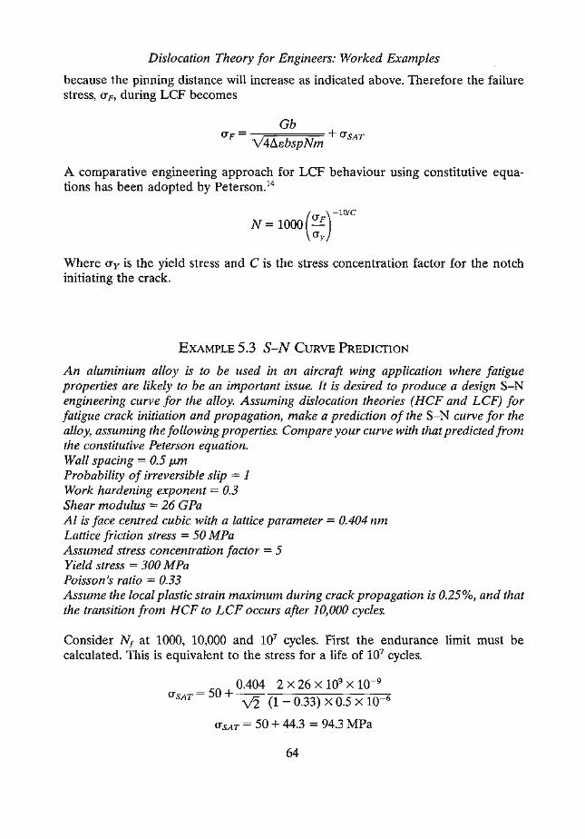
Dislocation Theory for Engineers: Worked Examples
because the pinning distance will increase as indicated above. Therefore the failurestress, (J"p, during LCF becomes
Cb(J" - + (J"
F - V4b.sbspNm SAT
A comparative engineering approach for LCF behaviour using constitutive equa-tions has been adopted by Peterson."
( )
-lOIC
N = 1000 ::
Where (J"y is the yield stress and C is the stress concentration factor for the notchinitiating the crack.
EXAMPLE 5.3 S-N CURVE PREDICTION
An aluminium alloy is to be used in an aircraft wing application where fatigueproperties are likely to be an important issue. It is desired to produce a design S-Nengineering curve for the alloy. Assuming dislocation theories (HCF and LCF) forfatigue crack initiation and propagation, make a prediction of the S-N curve for thealloy, assuming the following properties. Compare your curve with that predicted fromthe constitutive Peterson equation.Wall spacing = 0.5 JLmProbability of irreversible slip = 1Work hardening exponent = 0.3Shear modulus = 26 CPaAl is face centred cubic with a lattice parameter = 0.404 nmLattice friction stress = 50 MPaAssumed stress concentration factor = 5Yield stress = 300 MPaPoisson's ratio = 0.33Assume the local plastic strain maximum during crack propagation is 0.25%, and thatthe transition from HCF to LCF occurs after 10,000 cycles.
Consider N, at 1000, 10,000 and 107 cycles. First the endurance limit must becalculated. This is equivalent to the stress for a life of 107 cycles.
0.404 2 X 26 X 109 X 10-9(J"SAT = 50 + v2 (1 - 0.33) X 0.5 X 10-6
(J"SAT = 50 + 44.3 = 94.3 MPa
64

Dislocations in Fracture Processes
At 1000 cycles:
UF=
26 X 109 X 0.404 X 10-9
Vz + 94.3MPa0.404
4 X 0.0025 X 0.5 X 10-9 X 10-6 X 1000 X 0.7 X v'2
:. Up = 234 + 94.3 = 328.3 MPa
At 10,000 cycles:
Up = 74 + 94.3 = 168.3 MPa
Using the Peterson formula:
(328.3)-10/5
N = 1000 300 = 836 cycles
(168.3)-10/5
N = 1000 300 = 3177 cycles
Thus the S-N curve appears as in Fig. 5.8.15
400
100
,,,,,,,x-_
..................... --- --- --- ----~
350
300
8:.. 250~enenQ)
~ 200(ij.~·c::> 150
50 o Experimental data
X Theory (dislocation stress model)
o~----~----~------~----~----~o 200000 400000 600000 800000 1000000Number of cycles, N
Fig. 5.8 S-N curves for AI-Mg-Si alloy.IS
65

References
1. M. 1. WHELAN,Worked Examples in Dislocations, Institute of Materials, 1990.2. R. E. SMALLMAN,Modern Physical Metallurgy, 4th Edition, Butterworth, 1985.3. A. SEEGER,1. DIEHL, S. MEDER and K. REBSTOCK,Phil. Mag., 1957, 2, 323.4. G. R. ODETTEand D. FREY, J Nuclear Mat., 1979, 85-86, 818.5. 1. D. ESHELBY,F. C. FRANKand F. R. N. NABARRO,Phil. Mag., 1951, 42, 351.6. R. L. FLEISCHER,Acta Metall., 1963, 11, 203.7. N. F. MOTT and F. R. N. NABARRO,Report on the Strength of Solids, Physical Society,
1948, 1.8. V. GEROLDand K. HARTMANN,Trans. Japan Inst. Metals, 1968, 9, 509.9. H. 1. FROSTand M. F. ASHBY, Deformation Mechanism Maps - The plasticity and creep of
metals and ceramics, Pergamon Press, 1982.10. M. F. ASHBY,Phil Mag., 1966, 14, 1157.11. M. F. ASHBYand 1. D. EMBURY,Scripta Met., 1985, 19, 557.12. S. N. GHAFOURI,R. G. FAULKNERand T. E. CHUNG,Materials Science and Technology, 1986,2,
1223.13. H. MUGHRABI,Proc. Conf. on Dislocations and properties of real materials, Institute of Metals,
1985, 244-262 ..14. R. E. PETERSON,Stress concentration design factors, John Wiley, 1966.15. T. E. CHUNGand R. G. FAULKNER,Materials Science and Technology, 1990,6,1187.
67
