discussion paper no. 4238
TRANSCRIPT
DI
SC
US
SI
ON
P
AP
ER
S
ER
IE
S
Forschungsinstitut zur Zukunft der ArbeitInstitute for the Study of Labor
Analyzing Female Labor Supply:Evidence from a Dutch Tax Reform
IZA DP No. 4238
June 2009
Nicole BoschBas van der Klaauw

Analyzing Female Labor Supply:
Evidence from a Dutch Tax Reform
Nicole Bosch CPB Netherlands Bureau of Economic Policy Analysis
Bas van der Klaauw
VU University Amsterdam, Tinbergen Institute, CEPR and IZA
Discussion Paper No. 4238 June 2009
IZA
P.O. Box 7240 53072 Bonn
Germany
Phone: +49-228-3894-0 Fax: +49-228-3894-180
E-mail: [email protected]
Any opinions expressed here are those of the author(s) and not those of IZA. Research published in this series may include views on policy, but the institute itself takes no institutional policy positions. The Institute for the Study of Labor (IZA) in Bonn is a local and virtual international research center and a place of communication between science, politics and business. IZA is an independent nonprofit organization supported by Deutsche Post Foundation. The center is associated with the University of Bonn and offers a stimulating research environment through its international network, workshops and conferences, data service, project support, research visits and doctoral program. IZA engages in (i) original and internationally competitive research in all fields of labor economics, (ii) development of policy concepts, and (iii) dissemination of research results and concepts to the interested public. IZA Discussion Papers often represent preliminary work and are circulated to encourage discussion. Citation of such a paper should account for its provisional character. A revised version may be available directly from the author.

IZA Discussion Paper No. 4238 June 2009
ABSTRACT
Analyzing Female Labor Supply: Evidence from a Dutch Tax Reform
Among OECD countries, the Netherlands has average female labor force participation, but by far the highest rate of part-time work. This paper investigates the extent to which married women respond to financial incentives. We exploit the exogenous variation caused by a substantial Dutch tax reform in 2001. Our main conclusion is that the positive significant effect of tax reform on labor force participation dominates the negative insignificant effect on working hours. Our preferred explanation is that women respond more to changes in tax allowances than to changes in marginal tax rates. JEL Classification: H24, J22, J38 Keywords: uncompensated wage elasticity, labor force participation, working hours,
endogeneity Corresponding author: Bas van der Klaauw Department of Economics VU University Amsterdam De Boelelaan 1105 NL-1081 HV Amsterdam The Netherlands E-mail: [email protected]

1 Introduction
Since the work by Heckman (1974) female labor supply is an important topic
for economic research. A substantial contribution to this literature was made
by Blundell, Duncan and Meghir (1998), who showed that changes in tax
rules can be used to estimate wage elasticities. They investigates a series of
modifications in marginal tax rates over a relatively long observation period.
A more recent literature focusses on the importance of financial incentives,
such as earned income tax credits, on labor force participation decisions (e.g.
Eissa and Hoynes, 2004). We contribute to this literature by investigating
the effects of a very substantial Dutch Tax reform in 2001.
In 2001, labor force participation rate of prime-age women in the Nether-
lands were close to those in the UK or US. However, part-time work among
women is in the Netherlands much more common than in any other OECD
country. Whereas, on average in the OECD about 25% of the prime-age
working women work less than 30 hours per week, this is over 55% in the
Netherlands (OECD, 2004). The high degree of part-time work allows for
substantial room of increasing labor supply. It is also generally believed that
female labor supply is more responsive to financial incentives than male labor
supply (e.g. Meghir and Phillips, 2008). Therefore, Dutch policy have a large
interest in stimulating female labor supply. This should increase economic
growth and deal with the costs of an ageing society. Indeed, one of the most
important motivations for the Dutch tax reform in 2001 was to make work
financially more attractive for women.
The key elements of the tax reform were reducing marginal tax rates,
and removing perverse incentives of tax allowances (particularly for women
with a high-income partner). The magnitude of the reduction in after-tax
wages differed substantially among income levels. Reduced marginal tax
rates might both affect the labor force participation decision and hours of
work decision. Furthermore, the tax reform replaced the allowance by a
tax credit, both transferable between partners. The transferability makes
this change more likely to affect participation decisions than labor supply
decisions. The transferability of the allowance caused that for women with
a high-income partner earning a low income might have been financially less
1

attractive than not working. The reason was that when working, women
had to use their own allowance at a low marginal tax rate, while when not
working it would be transferred to their partner with a higher marginal tax
rate. The change from allowance to tax credit may thus be considered as a
reduction in the fixed costs of working. Saez (2002) stresses the importance
of financial incentives on the decision to participate in the labor force. There
are therefore two relevant margins to investigate, labor force participation
(extensive margin) and hours of work (intensive margin).
In the empirical analyses, we focus on prime-age women who are either
married or cohabiting. Our empirical model is similar to the model used in
Blundell, Duncan and Meghir (1998). However, we study a much shorter
time period with a substantial tax reform rather than a series of tax modifi-
cations. Tax reforms provide ideal natural experiments to study the effect of
financial incentives on female labor supply (see Blundell and MaCurdy, 1999;
Eissa, 1995; and Eissa and Hoynes, 2004). Because the tax reform generates
exogenous variation in after-tax wages, it allows us to deal with the simul-
taneity of working hours and after-tax wages. This simultaneity can arise,
for example, because unobserved preferences or ability affect both wages and
working hours, or because working hours have due to the progressive tax sys-
tem, a direct effect on after tax wages. Obviously, the tax reform does not
depend on individual characteristics, past choices and working hours. In the
empirical model, the after-tax marginal wage will be instrumented using the
tax reform. Since the tax reform was introduced at one specific moment, we
should control for aggregated calendar time effects on working hours. Fur-
thermore, we exploit that the tax reform affected different groups differently
to deal with self-selection into employment.
In the empirical analyses we use the Dutch Labor Force Survey collected
by Statistics Netherlands, which is a repeated cross-section containing in-
formation on (weekly) working hours, and at detailed level information on
the socioeconomic structure of the household. We link this to the Social
Statistical Database on Jobs, which contains administrative information on
jobs and gross income. Finally, we add taxable income registered by the tax
offices. The overlapping period of the three databases is from 1999 to 2005.
However, we restrict the observation period to 1999-2003.
2

We find that the estimated uncompensated wage elasticity is about -0.15,
but not significantly different from 0. This seems to imply that the tax
reform which increased after tax hourly wages did not increase female labor
supply. However, the tax reform had a substantial positive effect on labor
force participation, which we attribute to the shift from allowance to tax
credit. Simulations with our estimated model show that the positive effect
on labor force participation dominates the negative effect of wages. Whereas
working women on average reduced weekly working hours by 0.13 hours, in
the full population average working hours increased by 0.36. The effect of
the tax reform is highest for the lowest-educated women and decreases in
level of education.
Our empirical results contradict most earlier studies finding that the un-
compensated wage elasticity is between 0 and 0.3 (see Meghir and Phillips,
2008; for a survey). In particular, our results differ from those found in
Blundell, Duncan and Meghir (1998). It should, however, be noted that they
report a conditional correlation between wages and working hours similar to
what we find. As a sensitivity analysis we also apply their grouping estima-
tor, which gives a positive and significant uncompensated wage elasticity in
the same order as found in Blundell, Duncan and Meghir (1998). The group-
ing estimator might be less appropriate in our setting since our observation
period contains a single tax reform rather than a series of tax modification.
This might also explain that the grouping estimators suffers from weak in-
strument problems, mainly because it contains many instrumental variables
which are insignificant in the first-stage regressions.
The outline of this paper is the following. Section 2 provides details about
the Dutch tax reform of 2001. Section 3 introduces the empirical model. In
Section 4 we discuss our data. Section 5 presents the estimation results. And
Section 6 concludes.
2 The Dutch tax reform
In this section we provide details about the Dutch tax system. We mainly
focus on elements relevant for this study, and particularly on changes which
occurred during the tax reform in 2001.
3

The Dutch tax system is an almost fully individualized progressive tax
system. Prior to 2001 all individuals had a general allowance and individuals
only paid taxes on income above the allowance. There are also additional al-
lowances for working and parenting, which we discuss below. Income above
the allowances is taxed according to four income brackets with increasing
marginal tax rates (including national insurance premiums). The tax al-
lowances thus yield a higher tax reduction for high-income individuals with
a higher marginal tax rate.
An important feature of the general allowance is that if the allowance
is not fully used, the unused share is transferred to the partner.1 Transfer-
ring the allowance is particularly beneficial if the partner’s income falls in
a brackets with a higher marginal tax rate. So working at a low income is
financially relatively unattractive for women with a high-income partner.
The tax reform of 2001 replaced the general allowance by a tax credit. A
tax credit is simply a reduction in the total amount of taxes that an indi-
vidual should pay, so independent of the marginal tax rate. Like the general
allowance also the tax credit is transferable between partners. However, if a
woman increases labor supply, it can never be the case that the total amount
of the tax reduction decreases. The tax reform thus removed some fixed costs
of working, because the tax credit does not impose any disincentive effects
of working at a low income.
The tax reform in 2001 also included a reduction of marginal tax rates.
Table 1 shows for each year the marginal tax rates for the four different
income brackets in the Dutch tax system. The most substantial reduction
occurred in the highest two brackets, where marginal tax rates were reduced
by 8 percentage-points. However, not only the marginal tax rates changed,
but also the cut-off points of the brackets shifted. Figure 1 shows the marginal
tax rates for different taxable incomes in 2000 and 2001.
The tax reform of 2001 replaced the general allowance by a tax credit,
and introduced new tax credits for parenting and the combination of working
and parenting. The tax credit for parenting is transferable, but amounts
to only 138 euro. The tax credit for working is more substantial, but not
transferable. If an individual earns up till 50 percent of the annual (full-
1Married and cohabiting couples have the same status in the Dutch tax system.
4

Table 1: Main characteristics of the tax system.
1999 2000 2001 2002 2003 2004 2005
General allowance∗ (in e) 4674 4646Tax credit∗∗ (in e) 1731 1752 1715 1881 1916
Marginal tax rates in % (including national Insurance premiums)Lowest income bracket 35.75 33.9 32.35 32.35 32.35 33.4 34.4Income bracket 2 37.05 37.95 37.6 37.85 37.85 40.35 41.95Income bracket 3 50 50 42 42 42 42 42Highest income bracket 60 60 52 52 52 52 52
Explanatory notes:∗ The general allowance reduces taxable income.∗∗ The tax credit reduces the amount of tax paid.
Figure 1: Marginal tax rates before and after the tax reform of 2001.
0
0,1
0,2
0,3
0,4
0,5
0,6
0,7
0 10000 20000 30000 40000 50000 60000 70000 80000
real taxable income
2001 2000
5

Figure 2: The after-tax income before and after the Tax reform of 2001.
0
5000
10000
15000
20000
25000
30000
35000
40000
45000
0 10000 20000 30000 40000 50000 60000 70000 80000
Before tax income
Aft
er t
ax in
com
e
2001 2000
time) minimum wage, the tax credit increases to 150 euro. Above this the
tax credit further increases to 900 euro at an income level equal to the annual
(full-time) minimum wage. The impact of the tax credit for working causes
the drop in marginal tax rates between 8000 and 16,000 euro shown in Figure
1. The average taxable wage of working women is about 15,000 euro, which
lies in the interval with the most substantial reduction in marginal tax rates.
The tax reform of 2001 reduced labor tax for all individuals. As can
be seen in Figure 2 at almost all taxable income levels the after-tax income
was higher after the reform. However, it should be noted that also some
deductables were abolished. To compensate for the reduction in labor tax,
the government increased consumer taxes from 17.5 to 19 percent.
3 Empirical model
This section presents our empirical model. The model describes weekly work-
ing hours and has strong similarities with the model used in Blundell, Duncan
and Meghir (1998).
We focus on how the after-tax marginal hourly wage wit of woman i in
6

year t causally affects her weekly working hours hit. Therefore, we investigate
the traditional labor supply model (e.g. Heckman, 1974)
hi,t = β0 + β1 log(wi,t) + xi,tβ2 + ξt + εi,t (1)
The vector xi,t contains observed individual characteristics such as demo-
graphic variables, cohort dummies, level of education, etc. And the function
ξt describes common macroeconomic trends in female labor supply.
Obviously, the key parameter of interest in β1. It is, however, well known
that using OLS to estimate equation (1) yields inconsistent estimators for
β1. The logarithm of the after-tax marginal hourly wage may be correlated
to the error term εi,t for a number of reasons. First, there may be reversed
causality. Working more hours increases annual taxable income, which causes
that individuals enter an income bracket with a higher marginal tax rate.
Second, the vector xi,t most likely not captures all relevant heterogeneity in
individual preferences or ability. If there is unobserved ability and more able
individuals earn higher wages and have a stronger preference for work, then
there is a direct relation between log(wi,t) and εi,t.
We use the tax reform of 2001 to deal with endogeneity of log(wi,t). The
tax reform provided some exogenous variation in after-tax marginal hourly
wage. Therefore, we add the first-stage regression
log(wi,t) = α0 + αi,1 · I(t ≥ 2001) + xi,tα2 + ζt + Vi,t (2)
The indicator function I(t ≥ 2001) describing the period after the tax reform
thus acts as instrumental variable. We allow the effect of the tax reform on
wages αi,t to be different for different types of individuals. In particular,
we will allow for separate αi,1 for different educational groups. It should be
noted that the indicator I(t ≥ 2001) is only a relevant instrumental variable if
common macroeconomic trends ξt and ζt are smooth functions over calendar
time. Our identifying assumption is thus that between 2000 and 2001 there
are no general abrupt shocks in female labor supply other than due to the
tax reform. This also implies that the tax reform should not be the response
of policymakers to a sudden change in female labor force decisions or shifts
in preferences. Although, indeed an important goal of the tax reform was to
7

stimulate female labor force participation, there was no unexpected change
in female labor supply in the period prior to the tax reform.
A second important issue is that both over time and due to the tax
reform, the composition of working women might have changed. Recall that
the tax reform included a shift from an allowance to a tax credit, which
reduced the fixed costs of working. Furthermore, there is an increasing trend
in employment rates among women. Finally, the decision to work might
directly be related to unobserved preferences and ability. The self-selection
into work is thus most likely not random and cannot be ignored. To control
for selective labor force participation Pi,t we add a probit model
Pr(Pi,t = 1) = Φ (γ0 + γi,1 · I(t ≥ 2001) + xi,tγ2 + ψt) (3)
Again we allow the tax reform to have a differential impact on the labor force
participation of women with different educational degrees. And we allow for
a smooth trend ψt in female labor force participation.
We follow the estimation procedure of Blundell, Duncan and Meghir
(1998), which is a control function approach. First, we estimate the reduced-
form models (2) and (3) using OLS on the sample of employed women and
maximum likelihood estimation on the full sample, respectively. This pro-
vides us the residuals V̂i,t from the first-stage regression for wages and the
inverse Mills ratios λ̂i,t =φ(γ̂0+γ̂i,1·I(t≥2001)+xi,tγ̂2+ψ̂t)Φ(γ̂0+γ̂i,1·I(t≥2001)+xi,tγ̂2+ψ̂t)
from the participation
probit. We add these as regressors in equation (1), which gives the second-
stage equation
hi,t = β0 + β1 log(wi,t) + xi,tβ2 + ξt + β3V̂i,t + β4λ̂i,t + Ui,t (4)
Estimating this model using OLS on the sample working women provides
consistent parameter estimates for β1. Because equation (4) includes two
correction terms, at least two exclusion restrictions are required. The tax
reform should thus not be restructed to having the same impact for all women
on the after tax marginal hourly wage and labor force participation (i.e. αi,1
and γi,1 should be allowed to be different for women with different levels
of education). We return to this issue in Subsection 4.2 when we discuss
8

the impact of the tax reform. Finally, we should include in the vector of
regressors xi,t the after-tax income of the husband. The tax reform affects
the income of the husband as well. If female labor supply decisions are related
to the husband’s after-tax income which is most likely the case, ignoring the
husband’s income would cause a direct correlation between the error terms
εi,t and the tax reform I(t ≥ 2001). This would violate the validity condition
for using the tax reform as instrumental variable.
The parameter of interest β1 should be interpreted as the uncompensated
wage coefficient. This can be translated into the uncompensated wage elas-
ticity of labor supply by dividing by working hours. In particular, we divide
by mean working hours of employed women h̄, so β1
h̄. The uncompensated
wage elasticity includes both the substitution and the income effect. A pos-
itive value of β1 implies that the substitution effect dominates the income
effect.
4 Data
4.1 Sample
In the empirical analyses we use a data set constructed from three separate
databases. The Dutch Labor Force Survey collected by Statistic Netherlands
is a repeated cross-section containing detailed information on socioeconomic
and demographic characteristics of households. This database contains infor-
mation on employment status and weekly working hours, but lacks wages and
income. Therefore, we use a unique identification code to merge the Dutch
Labor Force Survey with the Social Statistical Database on Jobs. This data-
base contains information reported by employers on gross wages and annual
working hours for about a random one-third of the working population. We
link a third database containing taxable income registered by the tax office.
The three databases share the observation period from 1999 until 2005.
We restrict the data to married or cohabiting women between age 20
and 50 whose education level is observed. Women should have a working
husband with a taxable income above 9000 euro. The latter restriction is
made to avoid complications with husbands transferring tax allowances and
9

tax credits to their working wives. Furthermore, if the husband works the
wive is not entitled to means-tested welfare benefits. In total 116,553 women
in the Labor Force Survey satisfy the criteria above.
The employment status of women reflects the moment of the survey. If a
woman is employed, she is asked to report her weekly working hours. Indi-
viduals should report their contractual hours, or if they are working without
a contract the average number of hours they work during a week. In total
75 percent of the women are employed, and they work on average 25 hours
per week.
Next, we use the Social Statistical Database on jobs to compute the gross
hourly wage, which is the gross annual wage divided by annual working
hours. Because the Social Statistical Database on Jobs contains only a ran-
dom one-third of the working population, we get three subsamples: (i) work-
ing women with observed hourly gross wages, (ii) working women without
observed wages and (iii) non-working women. To reduce measurement errors
in wages, we transfer women from subsample (i) to subsample (ii) if the gross
hourly wage is below 90 percent of the mandatory minimum wage or above
200 euro per hour.2
We add taxable income to our data set, and apply the existing tax rules
to translate taxable income in after-tax income. By dividing the (annual)
after tax income by annual working hours we obtain the average after-tax
hourly wage. In our empirical model the relevant wage rate is not the average
after-tax hourly wage, but the marginal after-tax hourly wage. To obtain the
marginal tax rate we increase annual working hours by 10 and increase the
taxable income proportionally. Next, we translate taxable income again in
after-tax income and divide the increase in after-tax income by 10. Again,
this is only for the one-third of the sample for which we observe annual
working hours in the Social Statistical Database on jobs. To remove outliers
from the data, we transfer women from subsample (i) to subsample (ii) if
their after-tax hourly wage is below 72 percent of the gross minimum wage
and above 160 euro per hour. Finally, women reporting to work over 48
2In the Netherlands the minimum wage is the same for all workers above age 23 andis formulated in terms of gross hourly wages. Below age 23 the minimum wage is age de-pendent. The minimum wage is corrected for inflation twice a year. In 2000 the minimumwage for those above age 23 was 6.41 euro per hour.
10

hours, which is the legal maximum number of working hours per week, and
women having an annual taxable income above 150,000 euro are transferred
from (i) to (ii).
We have corrected wages for inflation. This takes account of the increased
consumer tax in 2001. Indeed, in 2001 the inflation rate was higher than in
previous years and it dropped again in 2002.
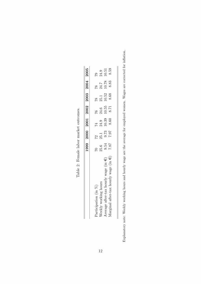
Table 2 reports some labor market outcomes. Female labor force partic-
ipation rates steadily increased between 1999 and 2003, and remained rela-
tively constant afterwards. During most of the period in which participation
rates increased, average working hours decreased. This suggests that those
women who newly enter the workforce, work relatively few hours. Finally,
both average and marginal after tax hourly wages express a substantial in-
crease in 2001. In 2004 wages again show some increase, which might have
been the result of the minor changes in the tax system implemented in 2004.
In the empirical analyses we only focus on the years 1999 until 2003, which
reduces the sample size by 34,614 women.
Individual characteristics are obtained from the Labor force Survey. Table
3 provides summary statistics both for working and non-working women.
Working women are on average slightly younger, have less (young) children
and are higher educated. Also the partners of working women are slightly
younger and on average higher educated. However, the after tax annual
income of partners with working women is on average more than 2000 euro
lower.
Table 4 shows for the different educational groups some characteristics of
the distribution of working hours by year. First, it should be noted that more
educated women are more likely to work and also more than 32 hours. For all
groups there is a negative trend in the percentage not working, however, the
fraction of women working more than 24 hours per week remain constant.
4.2 Impact tax reform on wages and participation
This subsection investigates the impact of the tax reform on after-tax wages
and on labor force participation. First, we provide some descriptive evidence.
Next, we focus on estimating the reduced-form models for the logarithm of
11
Tab
le2:
Fem
ale
labor
mar
ket
outc
omes
.
1999
2000
2001
2002
2003
2004
2005
Par
tici
pati
on(i
n%
)70
7274
7678
7879
Wee
kly
wor
king
hour
s25
.625
.124
.924
.625
.124
.724
.9A
vera
geaf
ter-
tax
hour
lyw
age
(ine
)9.
549.
7310
.39
10.5
510
.52
10.7
810
.51
Mar
gina
laf
ter-
tax
hour
lyw
age
(ine
)7.
877.
978.
608.
718.
688.
838.
59
Exp
lana
tory
note
:W
eekl
yw
orki
ngho
urs
and
hour
lyw
age
are
the
aver
age
for
empl
oyed
wom
en.
Wag
esar
eco
rrec
ted
for
infla
tion
.
12
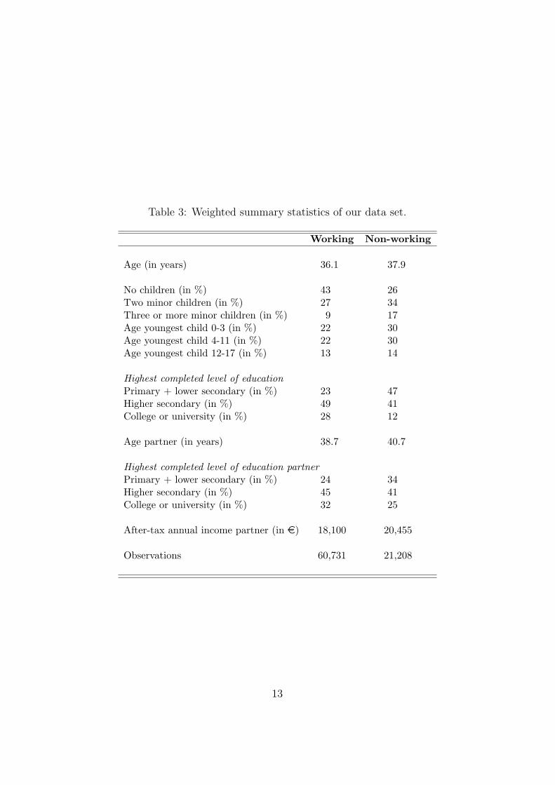
Table 3: Weighted summary statistics of our data set.
Working Non-working
Age (in years) 36.1 37.9
No children (in %) 43 26Two minor children (in %) 27 34Three or more minor children (in %) 9 17Age youngest child 0-3 (in %) 22 30Age youngest child 4-11 (in %) 22 30Age youngest child 12-17 (in %) 13 14
Highest completed level of educationPrimary + lower secondary (in %) 23 47Higher secondary (in %) 49 41College or university (in %) 28 12
Age partner (in years) 38.7 40.7
Highest completed level of education partnerPrimary + lower secondary (in %) 24 34Higher secondary (in %) 45 41College or university (in %) 32 25
After-tax annual income partner (in e) 18,100 20,455
Observations 60,731 21,208
13

Table 4: Fraction of women with particular working hours by year and edu-cational level.
No work ≤ 16 hours 16-24 hours 24-32 hours > 32 hours
Low education1999 44% 13% 19% 10% 14%2000 42% 15% 20% 9% 14%2001 39% 13% 22% 10% 15%2002 36% 15% 22% 12% 15%2003 37% 14% 21% 12% 17%
Medium education1999 26% 11% 24% 15% 25%2000 25% 11% 25% 16% 24%2001 22% 13% 26% 15% 24%2002 22% 13% 28% 16% 21%2003 21% 12% 27% 18% 22%
High education1999 16% 5% 21% 19% 39%2000 15% 6% 21% 19% 38%2001 14% 6% 22% 21% 37%2002 13% 6% 23% 20% 38%2003 11% 6% 21% 21% 41%
14

the after-tax marginal hourly wags and labor force participation (equations
(2) and (3) respectively).
Table 5 summarizes for each year the marginal tax rate, the after-tax
marginal hourly wage and the participation rate. Recall from Section 2 that
the tax reform has different impacts on marginal tax rates at different parts
of the income distribution. Therefore, we distinguish between low-educated,
medium-educated and high-educated women. For all three groups marginal
tax rates are substantially reduced due to the tax reform. The impact of the
tax reform is however smallest for the highest educated women.
The drop in marginal tax rates due to the tax reform causes a substantial
increase in after-tax marginal hourly wage for all groups. Participation rates
steadily increase during the observation period, but show for the low and
medium educated a jump in 2001. The impact of the tax reform thus seems
to be different for different educational groups. As we argued earlier the
tax reform is not correlated to individual preferences or unobserved ability.
However, for drawing inference it is not only necessary that the instrument
variables are not correlated to the error terms in the labor supply equation
(1), but they should also be relevant. The latter implies that the instruments
should have a sufficiently large impact on wages and labor force participation.
Table 6 reports the estimation results for the reduced-form equations (2)
and (3). The F -test for joint significance of the instrumental variables are 43
and 21, which is above the critical value for weak instruments mentioned by
Stock and Staiger (1997).3 In the participation equation there are some dif-
ferential impacts of the tax reform by educational group, but the differences
are not significantly (the p-value for similarity is 0.38). In the wage equation
the coefficients for the different educational groups are very similar and the
p-value for similarity equals 0.53.
5 Estimation results
In this section we first present the estimation results for the labor supply
model. Next, we perform simulations with the model. Finally, we discuss
3Note that the weak instrument literature focuses on linear models, while our first-stagemodel for labor force participation is non-linear.
15
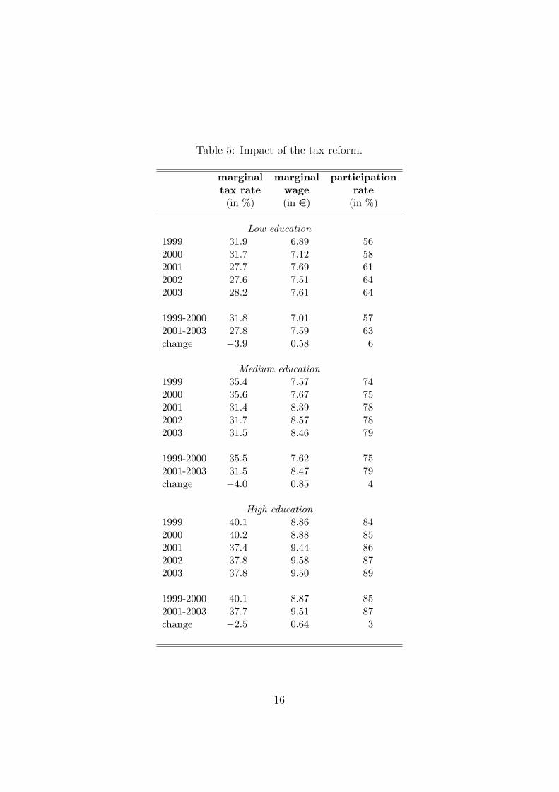
Table 5: Impact of the tax reform.
marginal marginal participationtax rate wage rate(in %) (in e) (in %)
Low education1999 31.9 6.89 562000 31.7 7.12 582001 27.7 7.69 612002 27.6 7.51 642003 28.2 7.61 64
1999-2000 31.8 7.01 572001-2003 27.8 7.59 63change −3.9 0.58 6
Medium education1999 35.4 7.57 742000 35.6 7.67 752001 31.4 8.39 782002 31.7 8.57 782003 31.5 8.46 79
1999-2000 35.5 7.62 752001-2003 31.5 8.47 79change −4.0 0.85 4
High education1999 40.1 8.86 842000 40.2 8.88 852001 37.4 9.44 862002 37.8 9.58 872003 37.8 9.50 89
1999-2000 40.1 8.87 852001-2003 37.7 9.51 87change −2.5 0.64 3
16

Table 6: Estimation results for the reduced-form equations.
participation log hourlywage
instrumental variableslow education post reform 0.103 (0.034) 0.078 (0.018)medium education post reform 0.100 (0.030) 0.080 (0.009)high education post reform 0.025 (0.051) 0.064 (0.011)
F -test for instruments 20.97 42.62
Observations 81,939 25,114
Explanatory note: Standard errors in parentheses. Controls added for education, cohort,calendar time, household situation, education and income of partner (see Table 10 for allparameter estimates).
some sensitivity analyses.
5.1 Parameter estimates
Table 7 presents the estimation results for the labor supply model. In the full
specification of the model (column (1)), the uncompensated wage elasticity
equals −3.87225.03
= −0.15. A negative wage elasticity implies that the income ef-
fect dominates the substitution effect. Our finding does not coincide with the
literature surveyed by Meghir and Phillips (2008). They mention that most
studies find an elasticity between 0 and 0.3. However, even at a 10% level,
our wage elasticity is not significant. But earlier studies for the Netherlands
found large and positive wage elasticities, for example, Van Soest, Woittiez
and Kapteyn (1990) estimated the wage elasticity to be 0.45. And Evers, De
Mooij and Van Vuuren (2008) conclude, based on surveying the literature,
that the wage elasticity for women in the Netherlands should be around 0.5.
It is important to stress that the instrumental variables approach mea-
sures a local average treatment effect (Imbens and Angrist, 1994). So we
estimate the uncompensated wage elasticity at the margin where the tax re-
17

Tab
le7:
Est
imat
ion
resu
lts
for
the
labor
supply
model
.
(1)
(2)
(3)
(4)
log
hour
lyw
age
−3.
872
(2.6
14)−
1.98
1(2
.561
)−
2.27
9(0
.221
)−
2.28
0(0
.221
)w
age
resi
dual
1.60
1(2
.625
)−
0.30
0(2
.572
)in
vers
eM
ills
−4.
016
(1.1
81)
−3.
873
(1.1
56)
Obs
erva
tion
s25
,114
25,1
1425
,114
25,1
14
Exp
lana
tory
note
:R
obus
tst
anda
rder
rors
inpa
rent
hese
s.C
ontr
ols
adde
dfo
red
ucat
ion,
coho
rt,
cale
ndar
tim
e,ho
useh
old
situ
atio
n,ed
ucat
ion
and
inco
me
ofpa
rtne
r(s
eeTab
le11
for
allpa
ram
eter
esti
mat
es).
18

form affects the after tax marginal hourly wage. Recall that the tax reform
had two important elements, marginal tax rates were reduced, and allowances
were transformed into tax credits. The second element caused that work be-
came financially more attractive for women with high income partners. Our
data show a large degree of assortative matching on education (the correla-
tion in level of education between partners is 0.45). However, if we look at
income, the correlation between partners is much smaller, only 0.06 in the
period before the tax reform. After the tax reform this correlation increased
to 0.09. After the tax reform women with high-income partners started to
earn more relative to women with low-income partners. However, we saw
from Table 4 that the fraction of women with many working hours remained
constant during the observation period. The tax reform thus caused women
with high-income partners to enter the labor force, but to work only few
hours. We attribute this mainly to the change from allowance to tax credit,
which removed some perverse incentives for working. Since the women who
newly enter the labor market have relatively good skills (due to assortative
matching), they can also earn relatively good wages, but devote fewer hours
to work than would be expected. This might explain why we estimate the
wage elasticity to be negative.
Our interpretation of the results is that the shift from general allowance
to tax credit was the part of the tax reform which yields the most substantial
incentive. In-work tax credit are often found to have stimulating effects on
the labor force participation decision of women (e.g. Aaberge and Flood,
2008; Eissa and Hoynes, 2004; Eissa and Liebman, 1996; and Meyer and
Rosenbaum, 2001). If indeed this shift was the key element of the tax re-
form, the impact of the reform might be different for women with partner’s
with high and low income. Therefore, we added as instrumental variable an
interaction between the reform and the partner’s income. However, while
having the expect signs the coefficients of this instrument in the first-stage
regressions were not significant and there were no changes in the results of
the second-stage regression.
The coefficient for the wage residuals is positive but not significant. There-
fore, we cannot reject that the after-tax marginal wage is exogenous. How-
ever, ignoring possible endogeneity in wages reduces the wage elasticity to
19

−2.270925.03
= −0.09 (see column (3)). Due to the substantial reduction in the
standard error this wage elasticity also becomes significant. The significant
coefficient of the inverse Mills ratio (in column (1)) means that there is self-
selection into work. The negative coefficient of the inverse Mills ratio implies
that women who participate in the labor markets are also women who are
more likely to work relatively many hours. Ignoring selective labor market
participation has roughly the same effect on the wage elasticity as ignoring
endogenous wages (see column (2)). Ignoring both selective labor market
participation and endogenous wages has about the same effect as ignoring
only one of theses potential sources of bias (column (4)). It is interesting to
note that this conditional correlation between wages and working hours is
very similar to what Blundell, Duncan and Meghir (1998) report.
In the baseline specification, other exogenous regressors (see Table 11)
are almost always significant and have the expected signs. Higher-educated,
younger and cohabiting women work more hours. Women with children
work less. However, working hours increase in the age of the youngest child,
but reduce in the number of children present in the family. Women with a
high-income partner work fewer hours. We have tried to include the partner’s
income squared to capture that the association between female working hours
and partner’s income might be nonlinear. But this term was not significant
and adding this term did not change the main parameters of interest.
5.2 Model simulations
Next, we perform some simulations to get insight in the effect of the tax
reform on female working hours. Table 8 shows the results of these simula-
tions for all women and also separately for low, medium and high-educated
women. In the simulations we use all women who are observed in the data
in the year 2001.
The first row of the table shows the situation in 2001 (so after the tax
reform). The labor force participation model predicts that 74.5 percent of
the women has a job. The average after-tax marginal hourly wage is 8.09
euro. Women who are working have on average 23.65 working hours per
week. However, in the full population the average number of working hours
20

Tab
le8:
Model
sim
ula
tion
s.
Par
tici
pat
ion
Aft
er-t
axH
ours
ofH
ours
ofra
tehou
rly
wag
epar
tici
pan
tsal
lw
omen
All
wom
enA
fter
tax
refo
rm74
.5%
8.09
23.6
518
.28
Onl
yta
xre
form
onpa
rtic
ipat
ion
74.5
%7.
5023
.94
18.4
9N
ota
xre
form
71.9
%7.
5023
.78
17.9
2
Low
educ
ated
Aft
erta
xre
form
61.0
%7.
3121
.18
13.3
7O
nly
tax
refo
rmon
part
icip
atio
n61
.0%
6.76
21.4
813
.56
No
tax
refo
rm57
.2%
6.76
21.2
412
.76
Med
ium
educ
ated
Aft
erta
xre
form
77.8
%8.
0823
.46
18.7
5O
nly
tax
refo
rmon
part
icip
atio
n77
.8%
7.46
23.7
618
.99
No
tax
refo
rm75
.0%
7.46
23.5
918
.35
Hig
hed
ucat
edA
fter
tax
refo
rm85
.7%
9.19
27.4
924
.02
Onl
yta
xre
form
onpa
rtic
ipat
ion
85.7
%8.
6227
.74
24.2
4N
ota
xre
form
85.2
%8.
6227
.71
24.1
1
21

is 18.28 hours per week. The second row of the table describes the case
where the tax reform only affects participation, but marginal wages remain
unaffected. To some extent this mimics the situation where marginal tax
rates remained as in 2000 and the tax reform only included a shift from
allowance to tax credit. Of course, participation rates remained unaffected,
but after-tax marginal hourly wages are lower. Since the wage elasticity is
negative, the reduced after-tax marginal hourly wages cause a slight increase
in working hours and thus also of working hours of labor force participants.
The third row describes the case in which the tax reform would not have
been implemented in 2001. It shows that labor force participation rates are
substantially lower and working hours of working women are slightly higher.
The last column of the table shows that the labor force participation effect
of the tax reform dominates the effect of wages. So the tax reform caused
average working hours (in the full population) to increase from 17.92 to 18.28.
The remainder of the table shows the same simulation separately for dif-
ferent education groups. For all three groups the tax reform increases labor
force participation, although the effect becomes smaller as the educational
level increases (and also labor force participation is already higher). In nom-
inal terms the tax reform has about the same impact on after-tax marginal
hourly wages of all three groups. However, since low-educated women have
on average the lowest wages, the relative impact on wages of the tax reform
decreases as education increases. For lower and medium-educated women
the positive effect of the increased labor force participation dominates the
negative effect of higher wages on average working hours in the full popu-
lation. However, the decrease for the highest-education group is relatively
small compared to the increase in working hours of both other groups.
5.3 Sensitivity analyses
In this subsection we present a number of sensitivity analyses. First, we
split the sample according to the presence of children. We distinguish three
groups of married women. The first group consists of women with at least
one child younger than age 12. The second group describes women with the
youngest child above age 12 and the third group contains women without
22

dependent children in the household. In the upper plane of Table 9 we show
the estimation results for these three groups.
It should be noted that only for the group with young children, there
do not seem to be problems with weak instruments. For both other groups,
the instruments seem particularly weak in the probit model for labor force
participation. Furthermore, it should be noted that for all groups we find
an insignificant wage elasticity. We take this as evidence that splitting the
sample into different groups generates too small subsamples and causes esti-
mators to become imprecise.
Next, we split the sample according to the age of the women. We distin-
guish between women under age 40 and above age 40. The second plane of
Table 9 shows the estimation results by age. Whereas for the younger age
group the effect of wages on hour of work is negative and significant, it is
positive (and insignificant) for the older age group. For younger women both
wages and labor force participation is endogenous, while this is not the case
for older women. A possible explanation is that older women are less flexible
on the labor market, they change jobs less often and have, therefore, also
less possibilities to change working hours (although it should be noted that
in the Netherlands there is some regulation that provides workers flexibility
to change working hours within their job).
Now we slightly modify the estimation method. First, we estimate the
participation equation. Next, we perform 2SLS on the labor supply equation
(and the wage equation) in which we include the inverse Mills ratio as exoge-
nous regressor. Following this estimation procedure should not change too
much as the only difference is that now also the inverse Mills ratio is included
wage equation. If the inverse Mills ratio would be linear in its index, this
estimation procedure would be equivalent to the control function approach
used so far. So if estimated coefficients are very different, this is evidence
that important non-linearities in the model are ignored. As is shown in col-
umn (6) of Table 9 there is only a very minor difference in the estimated
wage elasticity.
Next, we extend the observation period by also including data from 2004
and 2005, and to include quadratic terms in the time trends. This improves
the predictive power of the instruments in the first-stage regressions, but
23

Table 9: Sensitivity analyses.
(1) (2) (3)
log hourly wage 1.018 (3.865) 2.108 (7.920) −6.772 (4.097)wage residual −3.514 (3.880) −4.264 (7.943) 4.934 (4.116)inverse Mills 3.919 (2.018) −0.859 (3.911) −17.849 (3.089)
F -test statistic for instrumentswage equation 18.6 5.4 20.7participation 22.7 2.0 3.8
# of instruments 3 3 3observations 12,312 3211 9591
Explanatory note: Robust standard errors in parentheses.(1) Married women with young children (youngest child under age 12)(2) Married women with older children (youngest child between age 12 and 17)(3) Married women without dependent children.
(4) (5)
log hourly wage −10.263 (2.897) 7.859 (5.276)wage residual 7.846 (2.910) −9.803 (5.297)inverse Mills −9.401 (1.322) 0.437 (2.297)
F -test statistic for instrumentswage equation 29.3 12.9participation 10.4 9.9
# of instruments 3 3observations 15,163 9951
Explanatory note: Robust standard errors in parentheses.(4) Women below age 40.(5) Women above age 40.
24
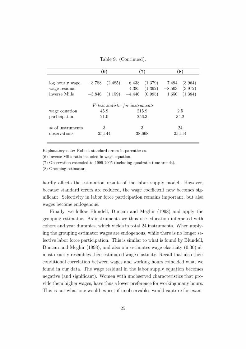
Table 9: (Continued).
(6) (7) (8)
log hourly wage −3.788 (2.485) −6.438 (1.379) 7.494 (3.964)wage residual 4.385 (1.392) −8.503 (3.972)inverse Mills −3.846 (1.159) −4.446 (0.995) 1.650 (1.384)
F -test statistic for instrumentswage equation 45.9 215.9 2.5participation 21.0 256.3 34.2
# of instruments 3 3 24observations 25,144 38,668 25,114
Explanatory note: Robust standard errors in parentheses.(6) Inverse Mills ratio included in wage equation.(7) Observation extended to 1999-2005 (including quadratic time trends).(8) Grouping estimator.
hardly affects the estimation results of the labor supply model. However,
because standard errors are reduced, the wage coefficient now becomes sig-
nificant. Selectivity in labor force participation remains important, but also
wages become endogenous.
Finally, we follow Blundell, Duncan and Meghir (1998) and apply the
grouping estimator. As instruments we thus use education interacted with
cohort and year dummies, which yields in total 24 instruments. When apply-
ing the grouping estimator wages are endogenous, while there is no longer se-
lective labor force participation. This is similar to what is found by Blundell,
Duncan and Meghir (1998), and also our estimates wage elasticity (0.30) al-
most exactly resembles their estimated wage elasticity. Recall that also their
conditional correlation between wages and working hours coincided what we
found in our data. The wage residual in the labor supply equation becomes
negative (and significant). Women with unobserved characteristics that pro-
vide them higher wages, have thus a lower preference for working many hours.
This is not what one would expect if unobservables would capture for exam-
25

ple motivation, work attitude or unobserved skills. Also Blundell, Duncan
and Meghir (1998) do not provide an explanation for this type of endogeneity.
A possible explanation for the difference between the results from the group-
ing estimator and our estimates presented in Table 7 is that the grouping
estimator contains many instruments and that the resulting wage elasticity
describes a mixture of many local average treatment effects.
We should also consider the first-stage regressions. Most instruments
are not significant in the first-stage regressions. However, the F -test for
joint significance of the instruments has both in the wage equation and the
labor force participation equation a p-value of less than 0.001 (which is what
Blundell, Duncan and Meghir (1998) report). The F -test statistic is however
small and in case of having many instruments indicates problems with weak
instruments (e.g. Stock and Yogo, 2005). Extending the observation period
by including also 2004-2005 (and thus taking account of the tax modifications
in these years) does not solve the weak instrument problem and also does
not change any of the estimation results.
6 Conclusions
In this paper we investigated how financial incentives affect female labor
supply. We focussed on the Netherlands, which has average female labor force
participation, but by far the highest rate of part-time work among women
within the OECD. This suggests that women carefully choose their working
hours (and within the Netherlands there is also some regulation that allows
for flexibility in adapting hours of work). We exploited exogenous variation
from a substantial tax reform in 2001. An important reason for the tax reform
was to induce women to increase labor supply. The tax reform included a
reduction in marginal tax rates and a change from allowance to tax credit
(which are both transferable). The latter removed some perverse incentives
for working. In the empirical analyses we combine three different databases
to construct a large data set covering the period around the tax reform. The
empirical results show a negative (but insignificant) uncompensated wage
elasticity, implying that the income effect dominates the substitution effect.
The tax reform does have a significant effect on labor force participation
26

and we also find significant selection effects. We attribute this to the change
from allowance to tax credit. This finding is in agreement with a large litera-
ture on earned income tax credits, which finds that the extensive marginal of
female labor supply is more sensitive to financial incentives than the inten-
sive margin. We performed some simulations with the estimated model and
found that the tax reform increased average weekly hours of work by 0.36,
which is about 2 percent of average working hours in the population.
27

References
Aaberge, R. and L. Flood (2008), Evaluation of an in-work tax credit reform
in Sweden: effects on labor supply and welfare participation of single
mothers, Working Paper 3736, IZA Bonn.
Blundell, R., A. Duncan and C. Meghir (1998), Estimating labor supply
responses using tax reforms, Econometrica 66, 827–861.
Blundell, R. and T. MaCurdy (1999), Labor supply: a review of alternative
approaches, in O. Ashenfelter and D. Card (eds.), Handbook of Labor
Economics, Volume 3A, North-Holland, Amsterdam.
Eissa, N. (1995), Taxation and labor suply of married women: the tax reform
of 1986 as a natural experiment, Working paper 5023, NBER.
Eissa, N. and H.W. Hoynes (2004), Taxes and the labor market participa-
tion of married couples: the earned income tax credit, Journal of Public
Economics 88, 1931–1958.
Eissa, N. and J.B. Liebman (1996), Labor supply responses to the earned
income tax credit, Quarterly Journal of Economics 111, 605–637.
Evers, M., R. de Mooij and D. van Vuuren (2008), The wage elasticity of
labour supply: a synthesis of empirical estimates, De Economist 156, 25–
43.
Heckman J.J. (1974), Shadow prices, market wages and labor supply, Econo-
metrica 42, 679–694.
Imbens, G.W. and J.D. Angrist (1994), Identification and estimation of local
average treatment effects, Econometrica 62, 467–475.
Meghir, C. and D. Phillips (2008), Labour Supply and Taxes, Discussion
Paper 3405, IZA Bonn.
Meyer, B.D. and D.T. Rosenbaum (2001), Welfare, The earned income tax
credit, and the labor supply of single mothers, Quarterly Journal of Eco-
nomics 116, 1063–1114.
OECD (2004), Female labour force participation: past trends and main de-
terminants in OECD countries, Economics Department Working Paper.
28

Saez, E. (2002), Optimal income transfer programs: intensive versus exten-
sive labor supply responses, Quarterly Journal of Economics 117, 1039–
1073.
Staiger, D. and J. Stock (1997), Instrumental variables regression with weak
instruments, Econometrica 65, 557–586.
Stock, J.H. and M. Yogo (2005), Testing for Weak Instruments in Linear IV
Regression, in D.W.K. Andrews and J.H. Stock (eds), Identification and
Inference for Econometric Models: Essays in Honor of Thomas Rothen-
berg, Cambridge University Press.
Van Soest, A., I. Woittiez and A. Kapteyn (1990), Labor supply, income
taxes, and hours restrictions in the Netherlands, Journal of Human Re-
sources 25, 517–558.
29
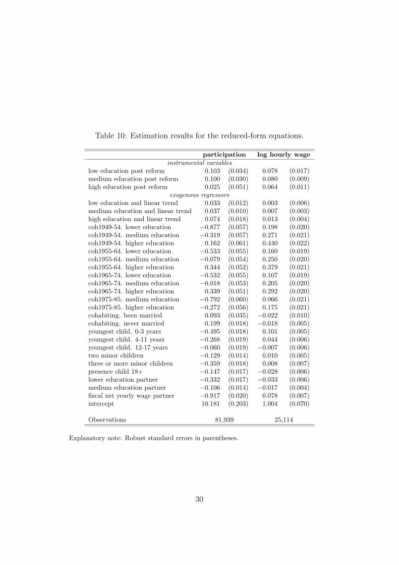
Table 10: Estimation results for the reduced-form equations.
participation log hourly wageinstrumental variables
low education post reform 0.103 (0.034) 0.078 (0.017)medium education post reform 0.100 (0.030) 0.080 (0.009)high education post reform 0.025 (0.051) 0.064 (0.011)
exogenous regressorslow education and linear trend 0.033 (0.012) 0.003 (0.006)medium education and linear trend 0.037 (0.010) 0.007 (0.003)high education and linear trend 0.074 (0.018) 0.013 (0.004)coh1949-54. lower education −0.877 (0.057) 0.198 (0.020)coh1949-54. medium education −0.319 (0.057) 0.271 (0.021)coh1949-54. higher education 0.162 (0.061) 0.440 (0.022)coh1955-64. lower education −0.533 (0.055) 0.160 (0.019)coh1955-64. medium education −0.079 (0.054) 0.250 (0.020)coh1955-64. higher education 0.344 (0.052) 0.379 (0.021)coh1965-74. lower education −0.532 (0.055) 0.107 (0.019)coh1965-74. medium education −0.018 (0.053) 0.205 (0.020)coh1965-74. higher education 0.339 (0.051) 0.292 (0.020)coh1975-85. medium education −0.792 (0.060) 0.066 (0.021)coh1975-85. higher education −0.272 (0.056) 0.175 (0.021)cohabiting. been married 0.093 (0.035) −0.022 (0.010)cohabiting. never married 0.199 (0.018) −0.018 (0.005)youngest child. 0-3 years −0.495 (0.018) 0.101 (0.005)youngest child. 4-11 years −0.268 (0.019) 0.044 (0.006)youngest child. 12-17 years −0.060 (0.019) −0.007 (0.006)two minor children −0.129 (0.014) 0.010 (0.005)three or more minor children −0.359 (0.018) 0.008 (0.007)presence child 18+ −0.147 (0.017) −0.028 (0.006)lower education partner −0.332 (0.017) −0.033 (0.006)medium education partner −0.106 (0.014) −0.017 (0.004)fiscal net yearly wage partner −0.917 (0.020) 0.078 (0.007)intercept 10.181 (0.203) 1.004 (0.070)
Observations 81,939 25,114
Explanatory note: Robust standard errors in parentheses.
30

Table 11: Estimation results for the labor supply model.
(1) (2) (3) (4)
log hourly wage −3.872 (2.614) −1.981 (2.560) −2.279 (0.221) −2.280 (0.221)wage residual 1.601 (2.625) −0.300 (2.572)Inverse Mills −4.016 (1.181) −3.873 (1.156)
exogenous regressorslow ed. and trend 0.103 (0.115) 0.181 (0.112) 0.067 (0.098) 0.189 (0.091)med. ed. and trend −0.136 (0.091) −0.086 (0.089) −0.179 (0.057) −0.077 (0.048)high ed. and trend −0.135 (0.099) −0.080 (0.098) −0.180 (0.066) −0.071 (0.058)coh1949-54. low ed. −4.326 (0.805) −5.036 (0.773) −4.653 (0.590) −4.977 (0.580)coh1949-54. med. ed. −1.822 (0.900) −1.538 (0.898) −2.224 (0.604) −1.457 (0.568)coh1949-54. high ed. 1.663 (1.270) 2.361 (1.255) 1.026 (0.722) 2.491 (0.590)coh1955-64. low ed. −2.143 (0.653) −2.129 (0.654) −2.384 (0.516) −2.082 (0.514)coh1955-64. med. ed. −0.438 (0.843) 0.269 (0.821) 0.791 (0.608) 0.344 (0.519)coh1955-64. high ed. 3.010 (1.137) 4.091 (1.095) 2.479 (0.727) 4.203 (0.532)coh1965-74. low ed. −0.848 (0.586) −0.741 (0.588) −1.005 (0.523) −0.709 (0.521)coh1965-74. med. ed. 0.122 (0.769) 1.003 (0.731) −0.159 (0.614) 1.064 (0.509)coh1965-74. high ed. 3.630 (0.956) 4.793 (0.900) 3.233 (0.697) 4.879 (0.518)coh1975-85. med. ed. 0.478 (0.603) 1.274 (0.562) 0.407 (0.591) 1.293 (0.535)coh1975-85. high ed. 2.291 (0.750) 3.165 (0.707) 2.064 (0.648) 3.215 (0.554)cohab., been married 3.357 (0.335) 3.555 (0.330) 3.397 (0.330) 3.549 (0.326)cohab., never married 2.093 (0.157) 2.349 (0.139) 2.130 (0.144) 2.344 (0.130)youngest child. 0-3 −6.855 (0.393) −7.738 (0.299) −7.021 (0.250) −7.707 (0.153)youngest child. 4-11 −6.730 (0.245) −7.175 (0.212) −6.814 (0.205) −7.162 (0.180)youngest child. 12-17 −4.009 (0.200) −4.040 (0.197) −4.000 (0.196) −4.042 (0.196)two minor children −2.368 (0.162) −2.616 (0.146) −2.393 (0.157) −2.613 (0.144)three or more kids −3.293 (0.284) −3.977 (0.198) −3.330 (0.277) −3.974 (0.197)presence child 18+ −2.132 (0.213) −2.315 (0.207) −2.097 (0.204) −2.324 (0.193)low. ed. partner −0.642 (0.220) −1.085 (0.177) −0.611 (0.214) −1.094 (0.159)med ed. partner −0.879 (0.130) −0.995 (0.125) −0.858 (0.126) −1.000 (0.118)net yearly wage part. −1.079 (0.532) −2.620 (0.285) −1.259 (0.443) −2.596 (0.196)intercept 49.789 (4.278) 59.300 (3.218) 48.610 (3.825) 59.590 (1.971)
Observations 25,114 25,114 25,114 25,114
Explanatory note: Robust standard errors in parentheses. Ed = education, med =medium, cohab = cohabiting.
31