discrimination of post-stack bright spots using avo and

Petroleum and Coal

Pet Coal (2019); 61(6) 1468-1478 ISSN 1337-7027 an open access journal

Article Open Access

DISCRIMINATION OF POST-STACK BRIGHT SPOTS USING AVO AND MODEL-BASED

INVERSION TECHNIQUE, COASTAL SWAMP NIGER DELTA, NIGERIA - A CASE STUDY D. E. Falebita*1, M. K. Saviour1, J. I. Jaiyeola2, O. A. Ojo1, A. A. Adepelumi1, 1 Department of Geology, Obafemi Awolowo University,Ile-Ife, Osun State, Nigeria 2 Nigerian Petroleum Development Corporation (NPDC), Benin, Nigeria

Received July 29, 2019; Accepted October 10, 2019

Abstract

Genuine hydrocarbon saturated post stack bright spots and the false ones have been discriminated using AVO and acoustic impedance attributes on the drill sites of three successful wells and delineated

prospects. Class III type AVO anomaly and low acoustic impedance are associated with the hydrocarbon sands. Concurrent regions with bright spots, AVO effect and low acoustic impedance are

identified as genuine bright spots indicating hydrocarbon sand while locations without the combination

of the three indicators are interpreted as false bright spots depicting shales or wet sand. The presence of a bright spot, high acoustic impedance and the absence of an AVO effect indicate prospect 2 (Well

A-4) to be a wet reservoir and shouldn’t have been drilled. While Prospect 1, which exhibits a bright

spot, good AVO effect and low acoustic impedance is interpreted as a hydrocarbon reservoir with a lateral extent of approximately 2 km and should be included in the next drilling program. This study

has, therefore confirmed the use of AVO analysis in generating prospects and reducing risks connected

with hydrocarbon exploration and development.

Keywords: Bright spot; AVO attributes; Acoustic impedance; Coastal swamp; Nigeria.

1. Introduction

Bright spot analysis is a direct hydrocarbon indicator technique premised on detecting anomalously higher amplitude in gas-bearing sediments compared to others [1]. However, many other geologic conditions can exhibit this characteristic which may lead to false bright spots and economic losses. AVO and model-based inversion techniques are used to extract

rock properties by discriminating seismic amplitudes for gas sands and wet sands [2]. In this particular example, four wells had been drilled based on post stack seismic bright spots in the coastal swamp area of western Niger Delta, Nigeria. Three of the wells (A-1, A-2, A-3) at the southeastern part encountered hydrocarbon but well A-4 drilled on a prospect at the central part was wet. This study is borne out of the need to reduce the ambiguity of geologic inter-pretation associated with new prospects being proposed for drilling by integrating AVO analysis

and model-based inversion. The results are expected to discriminate between genuine hydro-carbon saturated post stack bright spots and the false ones and consequently reduce overall exploration risks and costs.

2. Area description

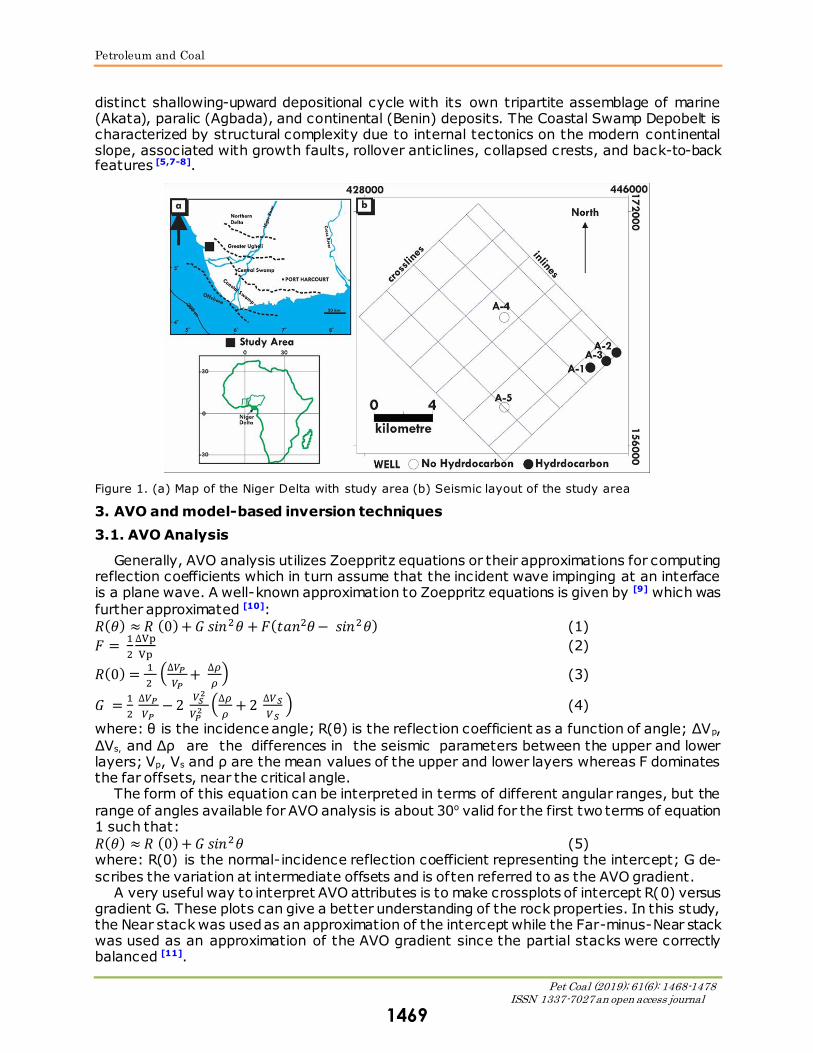
The study area (Figure 1) is located within the coastal swamp depobelt–one of the offlapping

siliciclastic sedimentation cycles that comprise the Niger Delta. These cycles prograde south-westward over oceanic crust into the Gulf of Guinea and are defined by synsedimentary fault-ing that occurred in response to the variable interplay of subsidence and sediment supply rates [3-5]. They define a series of punctuations in the progradation of this deltaic system and be-come successively younger basinward. The oldest lies furthest inland and the youngest is

located offshore [6]. These depobelts in order of decreasing age are Northern Delta, Greater Ughelli, Central Swamp, Coastal Swamp, and Offshore depobelts. Each depobelt contains a

1468

Petroleum and Coal

Pet Coal (2019); 61(6): 1468-1478 ISSN 1337-7027 an open access journal

distinct shallowing-upward depositional cycle with its own tripartite assemblage of marine (Akata), paralic (Agbada), and continental (Benin) deposits. The Coastal Swamp Depobelt is characterized by structural complexity due to internal tectonics on the modern continental slope, associated with growth faults, rollover anticlines, collapsed crests, and back-to-back features [5,7-8].

Figure 1. (a) Map of the Niger Delta with study area (b) Seismic layout of the study area

3. AVO and model-based inversion techniques

3.1. AVO Analysis

Generally, AVO analysis utilizes Zoeppritz equations or their approximations for computing reflection coefficients which in turn assume that the incident wave impinging at an interface is a plane wave. A well-known approximation to Zoeppritz equations is given by [9] which was

further approximated [10]:

𝑅(𝜃) ≈ 𝑅 (0) + 𝐺 𝑠𝑖𝑛2𝜃 + 𝐹(𝑡𝑎𝑛2𝜃 − 𝑠𝑖𝑛2𝜃) (1)

𝐹 = 1

2

∆Vp

Vp (2)

𝑅(0) =1

2 (∆𝑉𝑃

𝑉𝑃+

∆𝜌

𝜌) (3)

𝐺 =1

2 ∆𝑉𝑃

𝑉𝑃− 2

𝑉𝑆2

𝑉𝑃2

(∆𝜌

𝜌+ 2

∆𝑉𝑆

𝑉𝑆 ) (4)

where: θ is the incidence angle; R(θ) is the reflection coefficient as a function of angle; ∆Vp,

∆Vs, and ∆ρ are the differences in the seismic parameters between the upper and lower layers; Vp, Vs and ρ are the mean values of the upper and lower layers whereas F dominates the far offsets, near the critical angle.

The form of this equation can be interpreted in terms of different angular ranges, but the

range of angles available for AVO analysis is about 30o valid for the first two terms of equation 1 such that:

𝑅(𝜃) ≈ 𝑅 (0) + 𝐺 𝑠𝑖𝑛2𝜃 (5) where: R(0) is the normal-incidence reflection coefficient representing the intercept; G de-

scribes the variation at intermediate offsets and is often referred to as the AVO gradient. A very useful way to interpret AVO attributes is to make crossplots of intercept R(0) versus

gradient G. These plots can give a better understanding of the rock properties. In this study, the Near stack was used as an approximation of the intercept while the Far-minus-Near stack was used as an approximation of the AVO gradient since the partial stacks were correctly balanced [11].

1469

Petroleum and Coal


3.2. Model-based inversion

The model-based inversion (MBI) algorithm is an iterative procedure in which the imped-

ance is allowed to change gradually in such a way as to continuously improve the fit between the calculated synthetic trace and the real trace. It is a generalized linear inversion (GLI) algorithm that starts by perturbing a low-frequency model of the P-impedance until the seismic data approximates the computed synthetic trace within acceptable bounds. The low frequency P-impedance model is generated from well data and horizons. The output is then analyzed for gas or wet sands [2]. The approach is to minimize this function:

𝐽 = 𝑤𝑒𝑖𝑔ℎ𝑡1 × (𝑆 − 𝑊 ∗ 𝑟) + 𝑤𝑒𝑖𝑔ℎ𝑡2 × (𝑀 − 𝐻 ∗ 𝑟) (6)

where: S is the seismic trace; W is the wavelet; r is the final reflectivity; M is the init ial guess model impedance; H is the integration operator which convolves with the final reflectivity to produce the final impedance, and * is the convolution operator.

Minimizing the first part (S-W*r) forces a solution that models the seismic trace whereas

minimizing the second part (M-H*r), forces a solution that models the initial guess impedance by using the specified block size [12]. This is using the sparse reflectivity (SR) requirement [12] whereby the well log data is honoured for low frequency band; the layered geology is honoured for the high frequency band and the model that yields the least number of layers is chosen.

4. Analysis of rock and fluid properties

4.1. Seismic interpretation

The dataset includes a suite digital logs from five wells, 3D seismic partial angle stacks (Near, Far and Full stack) and migrated seismic data of approximately 156 km2 (Figure 1). The seis-

mic interpretation involved identification and correlation of reservoirs, seismic to well tie, as-sessment of data phase and polarity, identification of horizons at wells, recognition of minor and major faults on closely spaced vertical sections, determination of fault framework by tying vertical sections with horizontal sections and picking of horizons using the full offset data. These enabled the mapping of structural trapping mechanism and stratigraphic features. Fea-

tures of interest (bright spots) were enhanced using RMS horizon and window attributes.

4.2. Extracting AVO attributes

AVO attributes were derived from near and far stack volumes generated from pre-stack time migrated common-depth-point gathers. These gathers were reprocessed and corrected for normal moveout with Radon demultiple applied. The quality of the partial angle stacks was verified before performing any analyses on the data by constructing a crossplot of the near

and far stacks. The essence is to check if high near stack values are in accordance with high far stack values and that low near stack values are in accordance with low far stack values. This test reveals that the data are correctly balanced, well processed and the cross plot of near stack versus far minus near stack data is a good approximation of the crossplot between intercept and AVO gradient respectively. AVO anomalies are located by crossplotting a sizeable

window of data in the AVO gradient versus intercept of data planes and then looking for cluster points that stand out from the background majority of points [13-14]. The different segments on the near versus far-near cross plots were posted onto the AVO attributes time/depth win-dow, thereby creating an attribute volume. In order to study the reservoir laterally, the crossplot volume data was sliced along the horizons with the bright spot polygons superimposed on it [11].

4.3. Generating inversion models

The synthetic traces were calculated using the sonic and density logs with different wavelet types and frequencies for the three wells (A-1, A-4 and A-5) and compared to the composite traces (a single average trace around the borehole). The synthetic traces generated with a Ricker wavelet of 25 Hz dominant frequency gave the best correlation of 92% and were used

for subsequent inversion. The initial P-Impedance model used for the model based inversion was obtained from the density, sonic and horizons picked across the study area. The low-frequency component of this model was used to supply the low frequencies missing from the

1470

Petroleum and Coal


seismic. The model was filtered with a 10/15 Hz high cut frequency, and an acoustic imped-ance volume was generated for the analysis of fluid distribution across the study area.

5. Results and discussion

5.1. Structural and stratigraphic features

Figure 2a is a composite log comprising the Gamma Ray (GR) and Resistivity (RES_DEP) of wells A-1, A-2 and A-3 indicating three hydrocarbon reservoirs namely, RES-A, RES-B and RES-C identified within the Agbada formation. RES-A has a thickness ranging from 90 ft to 120 ft; RES-B has a thickness that varies between 50 ft and 60 ft while thickness values of

RES-C vary between 50 ft to 100 ft. The correlation displays series of shale/sand interbeds which have been deposited in the alternate cycle of regressive and transgressive systems, thus, forming reservoir/seal couplets where stratigraphic thinning and thickening of the sand intervals are recognized. A reliable seismic to well tie was obtained using Well A-5 (Figure 2b). The high goodness of fit obtained from the correlation of the synthetic seismogram with the real seismic traces depicts the reliability of the time-depth relationship used for the study.

Figure 2. (a) Correlation of pay zones at targeted prospect 2 at 9250ft and 9400ft responsible for the Bright Spot on Horizon 2 (b) Figure 2b: Dry Well A-5 with good seismic to well tie)

Figure 3 is the interpreted seismic section along inline 11993 showing horizons, amplitude anomaly and interpreted faults.

Figure 3. Interpreted Seismic Section of Prospect 1

1471

Petroleum and Coal


The faults (F1 (red), F2 (green), F3 (lemon) and F5 (pink)) are mainly structure building faults otherwise known as growth faults and

counter regional or antithetic faults characteristic of the Niger Delta. Most accumula-tions in the area are fault independent. A potential

prospect location–a structural high is identified within the broken circular red lines. Velocity analysis has been used to correct for the likely error of spurious velocity

pull-up due to inhomoge-neity in the low velocity layer (LVL) or gas shows between the surface and the reflector of interest. The pros-

pects are located at appro-ximately 8750 ft and 9250ft ft on horizon 1 and horizon 2 respectively (Figs. 4a and 4b).

Figure 4. (a) Depth Structure

Map (feet) of Horizon 1. Prospect

1 is marked (b) Depth Structure Map (feet) of Horizon 2 showing

Prospect 2

5.2. RMS amplitude and bright spots

The red ellipse on the seismic section of Fig. 3 shows bright spots around anticlinal struc-tures within the time intervals of -1750 and –2500 ms for the tops of hydrocarbon sands

Horizon 1 (lemon) and Horizon 2 (green) respectively. Examination of the RMS amplitude maps (Figs. 5a, 5b and 5c) reveals locations with anomalously high amplitudes which may be indicative gas, lithology or facies changes. Six bright spots-A, B, C, D, E and F are delineated. In Figure 5a, bright spot (red polygon) covers the locations of wells A-1, A-2 and A-3 (repre-senting existing discoveries). In Figure 5b, the blue polygon encloses bright spot A which

occurs on prospect 1, the magenta polygon encompasses bright spot B on the footwall of fault F1 while the red polygon surrounds bright spot C which is in close proximity to bright spot A. In Figure 5c, the blue polygon encompasses bright spot D while the magenta polygon sur-rounds bright spot E. Bright spots A and F conform to structure on prospect 1 and 2 respec-tively. Prospect 2 was the target of Well A-4, which turned out to be a dry well. This target was drilled based on the bright spot anomaly (Bright spot F) displayed on the amplitude map

(Figure 5b). The unsuccessful status of Well A-4 revealed that these bright spots could be diagnostic of other geologic conditions.

1472

Petroleum and Coal


Figure 5. (a) RMS Attribute Map showing a bright Spot at the location of Wells A-1, A-3 and A-

2 (b) RMS Attribute Map of Horizon 1 showing prospect 1 and three bright spots (A, B and C), (c) RMS Attribute Map of Horizon 2 showing prospect 2 and three other brights spots (D, E and F)

5.3. AVO anomalies

The data was processed with a cyan-blue-white-red-yellow colour coded format, as sug-gested by [15]. The blue colours indicate reflections with negative polarity signifying a decrease in acoustic impedance while the red colours depict reflections with positive polarity corre-

sponding to increase in acoustic impedance coefficients between layers (Fig. 6a). The anom-alies are most visible on the Far-stack data (Fig. 6b) as indicated by the yellow polygon around 2200 ms. A closer look at the far stack section reveals that thinner beds are clearer compares to the near stack section. The reason that this phenomenon becomes clearer with offset is that at near offset the waves are proximately vertical and that the distance between two

events is thinner than one fourth of the wavelength. A flat spot absent on the Full offset stack (Fig. 6c) is revealed by the Far minus Near stack (Fig. 6d). A test of data quality confirms the Near and Far Stacks are correctly balanced and their difference can, therefore, approximate the AVO gradient (Fig. 7a). Figure 7b is a plot of near stack (intercept) against far-minus-near stack (AVO gradient) which suggests that reflections due to shales and brine sands exhibit a

relatively small range of orientations creating a dominant background trend (grey colour). The top of the hydrocarbon is in the third quadrant (red), and its base is in the first quadrant (yellow) depicting class III AVO anomaly. The Class III AVO anomalies represent soft sands saturated with hydrocarbons which fit well with the young unconsolidated clastic sediments with large fluid sensitivity typical of the Niger Delta [16].

1473

Petroleum and Coal


Figure 6. (a) Near stack (b) Far stack with AVO anomaly on Prospect 1 (c) Full Offset

Stack and (d): Far minus Near stack – A flat spot is identified on Prospect 1

Figure 7. (a) Quality Control of Partial Stacked Data (Near versus Far stack) (b) AVO Anomaly Crossplot (Near versus Far minus Near Stack) indicating Class III AVO Anomaly (c) AVO Crossplot Volume Section

of prospect 1 (d) AVO Crossplot Volume Section of prospect 2

1474

Petroleum and Coal


Figure 8. AVO Crossplot Volume Slice with polygons (a) at the location of hydrocarbon wells A-1, A-3 and A-2 (b) at the bright spot locations on horizon 1 and (c) bright spot locations on horizon 2

5.4. Fluid discrimination

The Figure 9a shows the initial P-Impedance model used for the model based inversion. The low-frequency component of this model was used to supply the low frequencies missing from the seismic. The model was filtered with a 10/15 Hz high cut frequency. The colour scale was modified to better display the range of impedances within the zone of interest. Figure 9b represents the inversion analysis at the well locations (A-4, A-5 and A-1). The parameters

from this stage were used to run the inversion on the entire volume. The left panel of this display in each well shows an overlay of three impedance curves: the original impedance in blue, the initial guess model in black, and the final inversion result in red. The second panel shows the synthetic traces calculated from this inversion result compared with the input seis-mic trace while the third panel shows the Error, which is the difference between the two pre-

vious sets of traces. Figure 9c is a plot of the P-Impedance after inversion versus the P-Impedance of the original log showing the correlation between the two logs. The fact that the correlation is high indicates that this inversion has yielded a good result. That is, an acoustic impedance trace consistent with the wavelet and the input seismic trace has been created. Figures 10a and 10b are the inverted seismic sections along in lines 11945 and 12312 respec-

tively, showing the horizons and well log within the zone of interest. A green-yellow-red-blue-magenta colour coded format was used. The green colours indicate zones with low acoustic impedance; the magenta colours depict regions with high acoustic impedance while the other colours represent intermediate acoustic impedances. The vertical axis is restricted to the Agbada formation within a time interval of 2000 ms to 2400 ms. In both sections, the pro-spective intervals have been indicated by polygons. The prospect 1 polygon encloses green

data points indicating a low acoustic impedance region interpreted as hydrocarbon sand while

1475

Petroleum and Coal


the prospect 2 polygon encloses cyan-blue-red data points depictive of a high acoustic imped-ance zone representing shale or wet reservoir. Lowering of impedance will be high in hydro-carbon sand compared to water bearing sand or shale [16-17]. By comparing the RMS attribute maps (Figs. 5a, 5b and 5c), AVO crossplot volume slices (Figs.8a, 8b and 8c) and acoustic impedance sections (Figs. 10a and b), genuine bright spots are differentiated from false bright

spots (Table 1). Concurrent regions with bright spots, AVO effect and low acoustic impedance are identified as genuine bright spots indicating hydrocarbon sand while locations without the combination of the three indicators are interpreted as false bright spots depicting shales or wet sand. Two genuine bright spots (A and C) and one false bright spot (B) were identified on horizon 1 while all the bright spots on horizon 2 (D and E) were interpreted to be false. At

bright spot F location, this interpretation tallies with the low resistivity contrast observed on the resistivity log of Well A-4 (Figure 2b).

Figure 9. (a) P-Impedance Model of Full Offset Data showing A-4 Well (b) Multi-Well Inversion Correlation

window for A-4, A-5 and A-1 Wells, and (c) correlation plot of inverted P-impedance vs original P-im-pedance

1476

Petroleum and Coal


Figure 10. (a) Acoustic Impedance Cross Section of Prospect 1 and (b) Acoustic Impedance Cross Section of Prospect 2

Table 1. Summary of final discrimination results

Polygon Bright spot AVO effect Acoustic impedance Decision

A Yes Yes Low Genuine

B Yes No High False

C Yes Yes Low Genuine D Yes No High False

E Yes No High False

F Yes No High False

6. Conclusion

Brights spots, AVO attributes and acoustic impedance volumes have been used to re-eval-uate the drill sites of three successful wells and prospects in the study area. Class III type AVO anomaly and low acoustic impedance are associated with the hydrocarbon sands studied. This anomaly type is evident on the Near stack and Far minus Near stack cross-plots, and Far

minus Near times Near attributes. Whilst the conventional seismic interpretation had suc-ceeded in predicting hydrocarbon in some areas, in others this was not the case. The integra-tion of AVO analysis and model-based inversion has established prospect 2 (the target of Well A-4) to be a wet reservoir indicating the relevance of these techniques in reducing exploration risks and costs. Prospect 1, which exhibits a bright spot, good AVO effect and low acoustic

impedance is interpreted as a hydrocarbon reservoir with a lateral extent of approximately 2 km and should be included in the next drilling program. Generally, two genuine bright spots and four false bright spots are distinguishable within the area of interest. The study has out-lined the importance of AVO analysis and model-based inversion techniques in boosting con-fidence level on prospects in area yet undiscovered.

Acknowledgements

The authors would like to thank the Department of Petroleum Resources for releasing the data for

this research. We are grateful for the research grant from the Nigerian Association of Petroleum Explo-

rationists (NAPE).

1477

Petroleum and Coal


References

[1] Young KT, and Tatham RH. Fluid discrimination of poststack “bright spots” in the Columbus Basin, offshore Trinidad. The leading edge, 2007; 26 (12): 1508-1515.

[2] Ahhinav KD, and Kharagpur IIT. Reservoir Characterization using AVO and Seismic Inversion

Techniques. 9th Biennial International Conference and Exposition on Petroleum Geophysics-Hyderabad 2012. P205.

[3] Stacher P. Present understanding of the Niger Delta hydrocarbon habitat. In M. N. Oti & G.

Postma (Eds.), Geology of deltas, 1995; (pp. 257–267). Rotterdam: A. A. Balkema.

[4] Doust H, Omatsola E. Niger Delta. In J. D. Edwards & P. A. Santogrossi (Eds.), Divergent/pas-sive margin basins (p. 239–248). American Association of Petroleum Geologists Bulletin Mem-

oir, 1990; 48.

[5] Evamy BD, Haremboure J, Kamerling P, Knaap W., Molloy FA, Rowlands PH. Hydrocarbon habitat of Tertiary Niger Delta. American Association of Petroleum Geologists Bulletin, 1978;

62, 1–39.

[6] Tuttle WLM, Brownfield EM, Charpentier RR. The Niger Delta Petroleum System. Chapter A: Tertiary Niger Delta (Akata-Agbada) Petroleum System, Niger Delta Province, Nigeria, Cameroon

and Equatorial Guinea, Africa. U.S. Geolgical Survey, Open File Report, 1999; 99-50-H.

[7] Dim CIP. Hydrocarbon Prospectivity in the Eastern Coastal Swamp Depo-belt of the Niger Delta Basin–Stratigraphic Framework and Structural Styles,” in Springer Briefs in Earth Sci-

ences, 2017.

[8] Unukogbon NO, Asuen GO, Emofurieta WO. Sequence stratigraphic appraisal: Coastal swamp depobelt in the Niger Delta Basin Nigeria. Global Journal of Geological Sciences, 2008; 6(2):

129–137.

[9] Ak, K, and Richards, P G. Quantitative Seismology: Theory and Methods. San Francisco: W. H. Freeman and Co., 1980, 27-30.

[10] Shuey RT. A simplification of the Zoeppritz equations, Geophysics, 1985; 50: 609-614

[11] Avseth P, Mukerji T, and Mavko G. Quantitative Seismic Interpretation. Cambridge University Press, 2005.

[12] Hampson Russell, STRATA Theory. Hampson-Russell Software Services Limited,1999; 44-60.

[13] Castagna JP, Swan HW, and Foster DJ. Framework for AVO gradient and intercept interpre-tation, Geophysics, Society of Exploration Geophysicists,1998; 63, 948–956.

[14] Ross CP, and Kinman DL. Non-bright spot AVO: Two examples. Geophysics, 1995; 60: 1398-

1408. [15] Alistair RB. Interpretation of Three-Dimensional Seismic Data. AAPG Memoir42, SEG investi-

gations in Geophysics. 9, ISBN13: 978-0-89181-374-3.

[16] Castagna JP, and Swan HW. Principles of AVO crossplotting: The Leading Edge, 1997; 16, 337-342.

[17] Dubey AK. (2012): Reservoir characterization using AVO and seismic inversion techniques.

9th Biennial International Conference and Exposition on Petroleum Geophysics, 2012; 205.

To whom correspondence should be addressed: Dr. D. L. Falebita, Department of Geology, Obafemi Awolowo Uni-versity,Ile-Ife, Osun State, Nigeria, E-mail [email protected]

1478

mailto:[email protected]

discrimination of post-stack bright spots using avo and

Documents