avo and velocity analysis - luminaluminageo.us/papers/sarkar, castagna, lamb (2001) avo and...

GEOPHYSICS, VOL. 66, NO. 4 (JULY-AUGUST 2001); P. 1284–1293, 15 FIGS., 1 TABLE.

AVO and velocity analysis

D. Sarkar∗, J. P. Castagna‡, and W. J. Lamb‡

ABSTRACT

Velocity analysis using semblance estimates velocitiesbased on a constant amplitude model for seismogramsand does not take amplitude variation with offset (AVO)into account. In the presence of AVO, the constant ampli-tude model becomes inaccurate, particularly for eventswhich exhibit polarity reversals.

An AVO sensitive velocity analysis procedure, whichis a generalization of the traditional semblance method,can be devised by giving an offset dependence to themodeled seismograms. Incorporating AVO into veloc-ity analysis requires additional parameters to describethe reflectivity. This results in reduced velocity precision.By introducing a regularization term which provides acontrolled suppression of the contributions due to AVOeffects, we describe an AVO sensitive velocity analysisalgorithm that properly deals with events exhibiting po-larity reversals or large amplitude variation with offset.

INTRODUCTION

Semblance-based coherency measures are commonly ap-plied to perform velocity analysis (Taner and Koehler, 1969;Neidell and Taner, 1971) on seismic reflection data. Veloci-ties are estimated by maximizing a coherence functional or,equivalently, by minimizing the difference between the dataand an a priori amplitude distribution while varying the ve-locity. Thus, assuming a wrong a priori amplitude-versus-offset(AVO) function results in an incorrect velocity estimation. Asa result, amplitude variation with offset and velocity analysisare intimately related. Just as the wrong velocity gives incorrectAVO parameters, the converse (estimating the wrong velocityby assuming wrong AVO parameters) is also true, althoughthe latter exhibits itself in a more subtle way. This problem is

Presented at the 69th Annual International Meeting, Society of Exploration Geophysicists. Manuscript received by the Editor October 15, 1999;revised manuscript received July 31, 2000.∗Formerly University of Oklahoma, Institute for Exploration and Development Geosciences, Norman Oklahoma 73019; presently Colorado Schoolof Mines, Department of Geophysics, Golden, Colorado 80401. E-mail: [email protected].‡University of Oklahoma, Institute for Exploration and Development Geosciences, Norman, Oklahoma 73019. E-mail: [email protected]; [email protected]© 2001 Society of Exploration Geophysicists. All rights reserved.

particularly crucial for polarity reversals [such as may occurat the tops of some class 1 and class 2 sands (Rutherford andWilliams, 1989)]. Taking AVO effects into account should im-prove normal moveout (NMO) corrections and determinationof prestack attributes.

Semblance is today, as it has been for many years, the mostwidely used method of velocity analysis. It is robust and com-putationally efficient. Software is well developed and is readilyavailable. However, because it implicitly assumes a constantamplitude model, it does not handle AVO properly.

More recently, other methods have been developed. Thedifferential semblance method (e.g., Symes and Kern, 1994)works by comparing each trace with traces of similar offset (seeAppendix A). It eliminates secondary maxima and produces abroad primary maximum. Because it compares only traces ofsimilar offset, this method is less sensitive to AVO variationsthan traditional semblance analysis.

Eigenvalue methods (e.g., Biondi and Kostov, 1989; Key andSmithson, 1990) use the fact that the signal covariance matrixis of low rank in the absence of noise. These methods promisehigh resolution but in general are computationally more inten-sive than semblance. They easily incorporate AVO, even forcomplex variations (Appendix B). In principle, crossing andinterfering events can be handled (Biondi and Kostov, 1989),but great simplification in computation results from assuminga single event (Key and Smithson, 1990). Less is known aboutthe coherent noise immunity of these methods compared withthe vast experience of the geophysical community with sem-blance. Kirlin (1992) proposed a method intermediate betweeneigenvalue methods and semblance. It has the same limitationsas semblance with regard to AVO.

In this paper, we focus on generalizing the semblance methodso that it incorporates AVO. To develop a procedure similar tothe traditional semblance method and simultaneously accountfor amplitude changes with offset, we follow Corcoran andSeriff (1989) and define an objective function, �(vs | to), for agiven stacking velocity vs and zero offset time to, as

1284

Downloaded 16 Oct 2012 to 75.148.212.146. Redistribution subject to SEG license or copyright; see Terms of Use at http://segdl.org/

AVO and Velocity Analysis 1285

�(r [vs], vs | to) = 1

−

t=to+W�T∑t=to−W�T

‖(FM(r [vs], vs | t) − FD(vs | t))‖2


‖(FD(vs | t))‖2

, (1)

where FM and FD are the model and data vectors at a zerooffset time t and stacking velocity vs. ‖.‖ implies the L2 norm.The offset dependence is implicit in the vector norms. The ar-guments to the right of the vertical bar are treated as fixedparameters, whereas those to the left of the vertical bar areestimated. The objective function is the least squares fit of themodeled reflection amplitude to the data for a given velocity.To stabilize the problem against noise, the objective function

�(A, B,C, vs | to) = 1 −


N∑i=1

(A(vs | t) + B(vs | t) sin2 θi + C(vs | t) sin2 θi tan2 θi − FD(vs | xi , t)

)2


N∑i=1

(FD(vs | xi , t))2

. (3)

was calculated over a time window of (2W + 1) samples cen-tered at a particular zero offset time (to). This window shouldbe such that its length is inversely proportional to the frequencycontent of the data and approximately equal to the length ofthe wavelet. �T is the sample rate; r [vs] are the parameters thatdescribe the amplitude variation at a stacking velocity vs . Forexample, in the Shuey (1985) approximation to the Zoeppritzequations, r [vs] represents the AVO intercept and gradientterms. It can be shown that when FM is a least squares fit tothe data, � lies between 0 and 1. We refer to this function asthe generalized semblance function.

N∑i=1

FD(vs | xi , t)N∑i=1

FD(vs | xi , t) sin2 θ

N∑i=1

FD(vs | xi , t) sin2 θ tan2 θ

=

NN∑i=1

sin2 θi

N∑i=1

sin2 θi tan2 θi

N∑i=1

sin2 θi

N∑i=1

sin4 θi

N∑i=1

sin4 θi tan2 θi

N∑i=1

sin2 θi tan2 θi

N∑i=1

sin4 θi tan2 θi

N∑i=1

sin4 θi tan4 θi

A(vs | t)B(vs | t)C(vs | t)

, (5)

Corcoran and Seriff (1989) suggested giving an offset depen-dence to the amplitude in the forward model to account forAVO. The offset dependence is incorporated in the FM vector.Traditional semblance can be shown to be a particular case ofthis generalized procedure. However, we show here that whilethis process is accurate, it has less velocity precision than tra-ditional semblance when there is no amplitude variation withoffset. The results can be improved by treating the problemas a mixed determined problem (Menke, 1984). We show thatthis provides a general procedure to move from traditionalsemblance to an AVO sensitive semblance by varying a regu-larization parameter. This parameter determines the balancebetween robustness and accuracy of the algorithm.

In the subsequent paragraphs, we outline the amplitude de-pendent semblance in detail and show some applications tosynthetic and field data.

AVO SENSITIVE SEMBLANCE

Based on Corcoran and Seriff (1989), we describe anamplitude-dependent semblance procedure that is accurate inthe presence of AVO. Using Shuey’s (1985) approximation forthe reflection coefficient, the forward modeling operator at aparticular zero offset time t for data moved out at velocity vscan be written as

FM(vs | xi , t) ≈ A(vs | t) + B(vs | t) sin2 θi + C(vs | t)× sin2 θi tan2 θi , (2)

where θi = average angle of incidence and refraction at theith offset. It is a function of offset and depth. A is the AVOintercept, B is the AVO gradient, and C is the AVO curvature.The objective function can be written as

For a particular stacking velocity, vs, the reflectivity depends onthree coefficients A(vs |t), B(vs |t) andC(vs |t), and one needs tooptimize these coefficients as a function of vs. That is, A(vs |t),B(vs |t), andC(vs |t) must be determined at each trial velocityvs . To satisfy the optimization conditions, the derivatives withrespect to A(vs |t), B(vs |t), andC(vs |t) are equated to zero:

∂�

∂A(vs | t) = ∂�

∂B(vs | t) = ∂�

∂C(vs | t) = 0, (4)

and A(vs | t), B(vs | t), andC(vs | t) are solved using the follow-ing set of equations:

where N is the number of offsets in the seismogram. The sub-script i denotes the ith component of the vector.

The three equations are solved to obtain the best valuesof A(vs | t), B(vs | t), andC(vs | t) for a particular stacking ve-locity. When only one parameter, A, is used to fit the data,equation (5) becomes a linear equation in one unknown. Thenthe value of A that maximizes the objective function for aparticular velocity vs is the normalized stack trace given byA(vs | t) = 1

N

∑Ni=1 FD(vs | xi , t). On substituting this normal-

ized value of A in equation (3) we get

�(A, vs | to) =

1N


(N∑i=1

FD(vs | xi , t))2


N∑i=1

F2D(vs | xi , t)

, (6)


1286 Sarkar et al.

which is the familiar ratio of the average stacked energy to thetotal energy of its components—also called semblance. Tradi-tional semblance (A semblance) implicitly assumes a modelwith no change in amplitude with offset and where the con-stant amplitude A is the normalized stacked trace for a partic-ular trial velocity. This is accurate when AVO is negligible. AsAVO variations increase, the value of the traditional semblanceobjective function gradually decreases. At the extreme case ofa polarity reversal at the center of the offset range, the averagestack energy tends to zero without affecting the total energy ofits components. This gives rise to the misleading conclusion ofa fitness value tending to zero at the correct velocity.

In an attempt to improve on this, the slope (gradient) term,B, and the curvature term, C , are introduced in the reflectivityfunctional. In doing so we obtain better fits in the presenceof AVO and especially in the presence of polarity reversals.When A (intercept) and B (gradient) terms are used, we call themethod “AB semblance,” and when A, B, and C (curvature)terms are used, we call it “ABC semblance.” For our purposethe problem is simplified by (1) assuming hyperbolic moveoutsand (2) using a straight ray approximation instead of the correctincidence angles. However, these simplifications can be relaxedfor more complex problems.

INITIAL SYNTHETIC EXAMPLES

The first data set studied was a synthetic three-layer modelas shown in Figure 1 and Table 1. The first event has a polarityreversal near the center of the offset range, whereas the secondand third events have negligible AVO but opposite polarities.At the first interface, a decrease in Poisson’s ratio causes anegative B, whereas the P-wave velocity and density increasecauses a positive A. At the second interface, an increase inPoisson’s ratio gives a positive B, whereas an increase in P-wavevelocity and density gives a positive A. At the third interface, adecrease in Poisson’s ratio, P-wave velocity, and density gives anegative B and a negative A. The fitness curves obtained for thedifferent methods when applied to events 1 and 3 of Figure 1are shown in Figures 2 and 3, respectively.

Of special importance is the failure of the traditional sem-blance (A semblance) method to determine the correct velocityin the presence of a polarity reversal (Figure 2). This shows thatusing the wrong functional to describe the amplitude variationcan cause poor velocity determination. The fitness functioncurves for the third event (Figure 3) show that, in the absence ofstrong AVO variations, traditional semblance (A semblance) ismore robust than AB or ABC semblance. Figures 2 and 3 showthat there are basically two effects that couple together to de-termine the fitness function curve. The first effect is time depen-dent. It is the well-known effect of losing precision with depthbecause of the flattening of the moveout curve. The secondeffect is amplitude variation. When fewer parameters are

Table 1. Elastic parameters used to generate the synthetic seismogram shown in Figure 1.

Vp(P-velocity) (m/s) Vs(S-velocity) (m/s) ρ(density) (g/cm3) σ (Poisson’s ratio)

Layer 1 2500 982.759 2.192 0.4086Layer 2 2780 1853.334 2.251 0.09999Layer 3 3300 1672.414 2.349 0.3272Layer 4 2780 1853.334 2.251 0.09999

used than necessary, the fitness function optimizes at a wrongvelocity causing poor velocity estimation (Figure 2). Also,if more parameters than necessary are used, then preci-sion is lost as indicated by a flattening of the fitness curves(Figure 3).

FIG. 1. Synthetic gather consisting of three events. From top tobottom: event with a polarity reversal, and events with almostno AVO.

FIG. 2. Fitness plot for event 1 with polarity reversal, calculatedat the center of the event. Curves are semblance (A semblance),AB and ABC semblance, simple differential semblance (Ap-pendix A), and modified Key and Smithson (1990) coherence(Appendix B).



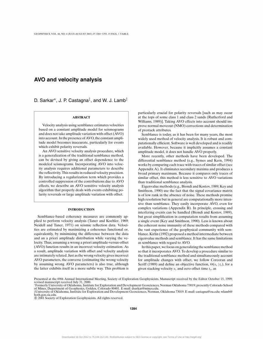
In Figures 2 and 3 we have also included fitness curves forsimple differential semblance (Appendix A) and a modifiedKey and Smithson (1990) eigenvalue method (Appendix B).The essential point is that both have maxima at the correct ve-locity, regardless of the presence or absence of AVO. The dif-ferential semblance curve is much broader and the eigenvaluemethod much sharper than the semblance family of curves.Care should be used in relating the sharpness of these curvesto velocity resolution. Because the normalization of the eigen-value and semblance methods are different, visual comparisonscan be misleading (Kirlin, 1992).

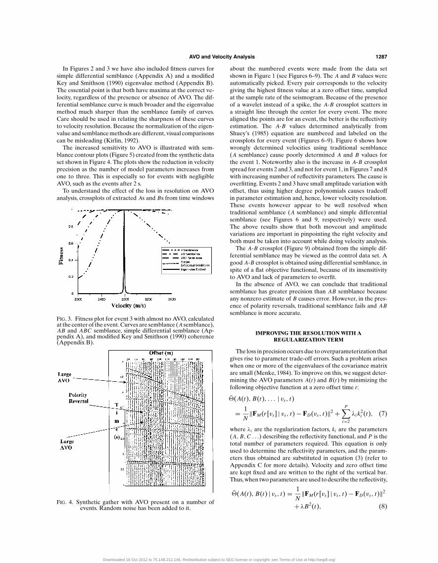
The increased sensitivity to AVO is illustrated with sem-blance contour plots (Figure 5) created from the synthetic dataset shown in Figure 4. The plots show the reduction in velocityprecision as the number of model parameters increases fromone to three. This is especially so for events with negligibleAVO, such as the events after 2 s.

To understand the effect of the loss in resolution on AVOanalysis, crossplots of extracted As and Bs from time windows

FIG. 3. Fitness plot for event 3 with almost no AVO, calculatedat the center of the event. Curves are semblance (A semblance),AB and ABC semblance, simple differential semblance (Ap-pendix A), and modified Key and Smithson (1990) coherence(Appendix B).

FIG. 4. Synthetic gather with AVO present on a number ofevents. Random noise has been added to it.

about the numbered events were made from the data setshown in Figure 1 (see Figures 6–9). The A and B values wereautomatically picked. Every pair corresponds to the velocitygiving the highest fitness value at a zero offset time, sampledat the sample rate of the seismogram. Because of the presenceof a wavelet instead of a spike, the A-B crossplot scatters ina straight line through the center for every event. The morealigned the points are for an event, the better is the reflectivityestimation. The A-B values determined analytically fromShuey’s (1985) equation are numbered and labeled on thecrossplots for every event (Figures 6–9). Figure 6 shows howwrongly determined velocities using traditional semblance(A semblance) cause poorly determined A and B values forthe event 1. Noteworthy also is the increase in A-B crossplotspread for events 2 and 3, and not for event 1, in Figures 7 and 8with increasing number of reflectivity parameters. The cause isoverfitting. Events 2 and 3 have small amplitude variation withoffset, thus using higher degree polynomials causes tradeoffin parameter estimation and, hence, lower velocity resolution.These events however appear to be well resolved whentraditional semblance (A semblance) and simple differentialsemblance (see Figures 6 and 9, respectively) were used.The above results show that both moveout and amplitudevariations are important in pinpointing the right velocity andboth must be taken into account while doing velocity analysis.

The A-B crossplot (Figure 9) obtained from the simple dif-ferential semblance may be viewed as the control data set. Agood A-B crossplot is obtained using differential semblance, inspite of a flat objective functional, because of its insensitivityto AVO and lack of parameters to overfit.

In the absence of AVO, we can conclude that traditionalsemblance has greater precision than AB semblance becauseany nonzero estimate of B causes error. However, in the pres-ence of polarity reversals, traditional semblance fails and ABsemblance is more accurate.

IMPROVING THE RESOLUTION WITH AREGULARIZATION TERM

The loss in precision occurs due to overparameterization thatgives rise to parameter trade-off errors. Such a problem ariseswhen one or more of the eigenvalues of the covariance matrixare small (Menke, 1984). To improve on this, we suggest deter-mining the AVO parameters A(t) and B(t) by minimizing thefollowing objective function at a zero offset time t :

�̄(A(t), B(t), . . . | vs, t)

= 1N

‖FM(r [vs] | vs, t) − FD(vs, t)‖2 +P∑i=2

λi k2i (t), (7)

where λi are the regularization factors, ki are the parameters(A, B,C . . .) describing the reflectivity functional, and P is thetotal number of parameters required. This equation is onlyused to determine the reflectivity parameters, and the param-eters thus obtained are substituted in equation (3) (refer toAppendix C for more details). Velocity and zero offset timeare kept fixed and are written to the right of the vertical bar.Thus, when two parameters are used to describe the reflectivity,

�̄(A(t), B(t) | vs, t) = 1N

‖FM(r [vs] | vs, t) − FD(vs, t)‖2

+ λB2(t), (8)


1288 Sarkar et al.

where λ is a parameter which determines which AVO param-eter (A or B) is to be given more importance. When λ is 0,the parameters estimated from the objective function [equa-tion (8)] equals that of AB semblance, and when λ goes to ∞ (inthe examples considered, a λ = 10 approximates ∞), the pa-rameters estimated from the objective function [equation (8)]becomes that of traditional semblance.

To find the effect of λ for the data sets used, we experimentedwith a number of values of λ ranging from 0 to 10 on data setsshown in Figures 1, 4, 13, and 14. The most significant four plotsare shown. We found that, for the data sets considered here,a value of λ(0.006) consistently stabilizes the results to a greatextent and achieves the resolution comparable to traditionalsemblance for deeper events where AVO is weak, while at thesame time it works well for some of the shallower events withconsiderable amplitude variation. This can be seen in the ve-locity fitness plots shown in Figures 10 and 11. Also, semblancecontour plots of the synthetic data (Figure 4) shown in Fig-ure 12 illustrate the influence of λ on velocity analysis. Similarplots computed on processed field common midpoint(CMP)gathers are shown in Figures 13 and 14. The data has ampli-tudes compensated for spherical divergence and attenuation,multiples removed, and a bandpass filter applied. The gatherswere NMO corrected with velocities that maximized the sem-blance curves at times 1.4, 1.6, and 1.8 s. The event around 1.6 s,shown in Figure 14, is significantly overcorrected, whereasFigure 13 shows that appropriate values of λ flattens the eventcorrectly. This again shows the failure of traditional semblanceto estimate accurate velocities for such events.

In Figure 15, we show a crossplot of intercept and gradientterms extracted from the field gather using velocities that max-imized AB semblance (λ = 0) at every time sample between

FIG. 5. Semblance contour plots for (a) semblance (A semblance), (b) AB, and (c) ABC semblance when applied on the data shownin Figure 4.

1.4 and 1.8 s. This method may be used to estimate reflectivityparameters along with velocities simultaneously.

When velocity analysis is performed on CMP gathers, a rea-sonable value of λ must be determined first. The factors thatinfluence the estimate of λ are (1) the data, which includesthe signal and noise content, (2) number of offsets, which de-termines the number of data points, and (3) the geometry ofthe problem (offset to depth ratios). Since the geometry of theproblem can be assumed to remain reasonably constant forlarge areas, a single value of λ, or at the most a few λs, shouldbe sufficient for an entire data set.

FIG. 6. A-B crossplot for data shown in Figure 1 computed fromvelocities determined by A semblance.



DISCUSSION AND CONCLUSIONS

Our study shows the limitations that arise when amplitudevariation is ignored in velocity analysis, and also shows theproblems of using more complicated amplitude dependencethan is necessary. It shows the classic tradeoff between ac-curacy and robustness (or bias versus variance). Traditionalsemblance, though not quite accurate, is robust. However,the AVO-parameterized semblance, though not robust, can beaccurate.

AVO-parameterized semblance (1) can determine A and Bvalues simultaneously with velocity, (2) provides a coherencemeasure that is directly comparable to traditional semblance,and (3) requires a regularization term for routine application.

Because AVO parameters are sensitive to velocity errors (Bwas seen to be more sensitive to velocity than A), care must betaken in their interpretation. Though AB semblance may be

FIG. 7. A-B crossplot for data shown in Figure 1 computed fromvelocities determined by AB semblance.

FIG. 8. A-B crossplot for data shown in Figure 1 computed fromvelocities determined by ABC semblance.

used on single events, it is not as robust as traditional sem-blance for reflections with only small AVO variations. Treatingthe problem as a mixed determined problem allows one to getthe best of both traditional semblance (A semblance) and AVOsensitive semblance. AVO sensitive semblance with a regular-ization term has the potential of computing better stackingvelocities in certain specific, but important, cases, thus improv-ing the accuracy of the velocity analysis algorithm.

There are a few effects ignored in this study. The first is theeffect of tuning. Tuning affects correct determination of A-Bparameters and hence can affect velocity determination. Thisis more of a problem for AB semblance than for A semblance(traditional semblance). For such cases, the eigenvalue methodis particularly attractive (Biondi and Kostov, 1989). The secondeffect ignored is the angle of incidence used. For this analysis,

FIG. 9. A-B crossplot for data shown in Figure 1 computed fromvelocities determined by differential semblance.

FIG. 10. Fitness versus velocity plots for different values of λwhen applied on event 1 (polarity reversal) in the data setshown in Figure 1.


1290 Sarkar et al.

the angle was computed from the arc tangent of the depth tooffset ratio. In most cases, this underestimates the true angleof incidence. Although the angle of incidence does not greatlyaffect the determination of the zero offset reflectivity (A), ithas a serious effect on the gradient (B) term. From our limitedanalysis, the effect does not seem to be significant on the casesstudied, but it may prove relevant in certain instances.

FIG. 11. Fitness versus velocity plots for different values of λwhen applied on event 3 (almost no AVO) in the data set shownin Figure 1.

FIG. 12. Semblance contour plots for different values of λ whenapplied on the synthetic data shown in Figure 4. (a) λ = 0.0,(b) λ = 0.006, (c) λ = 0.05, (d) λ = 10.

FIG. 13. Processed CMP field gather after NMO correction. (a)λ = 0.0, (b) λ = 0.006.

FIG. 14. Processed CMP field gather after NMO correction. (a)λ = 0.05, (b) λ = 10.



FIG. 15. Crossplot of the intercept and gradient terms esti-mated from the field gather using velocities that maximizedAB semblance at every time sample within a time window of1.4–1.8 s for λ = 0.0.

Now that semblance has been generalized to include AVO ef-fects, an objective of future research will be to compare the per-formance of the different velocity analysis methods (AVO sen-sitive semblance, differential semblance, and eigenvalue meth-ods) in the presence of various kinds of coherent noises andAVO variations.

ACKNOWLEDGMENTS

Thanks to Antonio Ramos and Bob Baumel (Conoco)for helpful comments throughout this study. Thanks to John

APPENDIX A

A SIMPLE DIFFERENTIAL SEMBLANCE

The concept of differential semblance exploits the similaritybetween two adjacent traces by calculating the difference be-tween the two traces. It is based on the hypothesis that the rightvelocity will give the right moveout curve, causing the events toline up on adjacent traces and, hence, give the optimum of theobjective function. We define it as the summation of the dif-ference between pairs of traces. This concept is similar to thedifferential semblance optimization of Symes and Kern (1994).Following Siegfried and Castagna (1982), the differential sem-blance objective function between two adjacent traces i andi + 1 can be written as

�S(vS | t) = ‖�Si+1 − �Si‖2

2(‖�Si+1‖2 + ‖�Si‖2

) , (A-1)

where Si is the ith trace of a gather.Equation (A-1) can be simplified to

�s(vs | t) = 12

− ‖�Si+1‖‖�Si‖ cos θ

‖�Si+1‖2 + ‖�Si‖2, (A-2)

which is equivalent to

�s(vs | t) = 12

−(

r

1 + r2

)cos θ, (A-3)

where r is the ratio of the norms of the two adjacent traces. Ifthey have the same time dependence but have different am-plitudes, r is just the ratio of these amplitudes. θ is the anglebetween the two vectors Si and Si+1. As the two waveformsbecome similar in shape and amplitude, the value of the ob-jective function �s decreases or, in other words, the value of(r/1 + r 2) cos θ increases. For a perfect match, this term equals1/2, and �s equals zero. Similarly, when there are N traces, thedifferential semblance objective function is given by

�s(vs | t) = 1 − 2N − 1

N−1∑i=1

ri1 + r2

i

cos θi , (A-4)

where the constant 2 is inserted to scale the function to a max-imum fitness of 1; ri and θi are the amplitude ratio and thephase difference of the ith pair. The sum consists of two parts:an amplitude part [ri/(1 + r 2

i )] and a waveshape part (cos θi ).The waveshape part is the crosscorrelation between the traces.For a simple interface and reflections inside the precriticalrange, AVO does not affect the waveshape but it does affectthe amplitude. Also, the amplitude part is significantly affectedonly if the trace separation is large. When trace separation issmall, the overall amplitude variation of the event does notaffect the differential semblance function. The relative impor-tance of the amplitude and the waveshape can be selected by

Anderson (Exxon Mobil), who suggested our considerationof differential semblance. Thanks to Lynn Kirlin and twoanonymous reviewers for many suggestions in improving themanuscript. We also thank the OU Geophysical ReservoirCharacterization Consortium for financial support. Thanks toConoco Inc. for providing the field data set.

REFERENCES

Biondi, B. L., and Kostov, C., 1989, High resolution veloc-ity spectra using eigenstructure methods: Geophysics, 54, 832–842.

Corcoran, C. T., and Seriff, A. J., 1989, Method of processing seismicdata: European Patent 335450.

Gersztenkorn, A., and Marfurt, K. J., 1999, Eigenstructure-based co-herence computations as an aid to 3-D structural and stratigraphicmapping: Geophysics, 64, 1468–1479.

Key, S. C., and Smithson, S. B., 1990, A new method of event detectionand velocity estimation: Geophysics, 55, 1057–1069.

Kirlin, R. L., 1992, The relationship between semblance and eigen-structure velocity estimators: Geophysics, 57, 1027–1033.

Menke, W., 1984, Geophysical data analysis: Discrete inverse theory:Academic Press Inc.

Neidell, N. S., and Taner, M. T., 1971, Semblance and other coherencymeasures for multichannel data: Geophysics, 36, 482–497.

Rutherford, S. R., and Williams, R. H., 1989, Amplitude-versus-offsetvariations in gas sands: Geophysics, 54, 680–688.

Shuey, R. T., 1985, A simplification of the Zoeppritz equations: Geo-physics, 50, 609–614.

Siegfried, R. W., and Castagna, J. P., 1982, Full waveform sonic log-ging techniques: 23rd Ann. Logging Symp., Soc. Prof. Well LogAnalysts, I1–I25.

Symes, W. W., and Kern, M., 1994, Inversion of reflection seismo-grams by differential semblance analysis: Algorithm structure andsynthetic examples: Geophys. Prosp., 42, 565–614.

Taner, M. T., and Koehler, F., 1969, Velocity spectra—Digital computerderivation and applications of velocity functions : Geophysics, 34,859–881.


1292 Sarkar et al.

varying the exponents m and n in the following objective func-tion:

�s(vs | t) = 1 − 1N − 1

N−1∑i=1

(2

ri1 + r2

i

)m

cosn θi . (A-5)

For comparison with semblance, we want an objective func-tion which has a maximum when all traces are identical. Since�s is a minimum for this case, we work instead with 1 − �s ,which we refer to as simple differential semblance. Figures 2and 3 show 1 − �s , with n=m= 1.

APPENDIX B

EIGENVALUE METHODS AND AVO

Eigenvalue methods (e.g. Biondi and Kostov, 1989; Key andSmithson, 1990) attempt to provide higher resolution than sem-blance. The key to understanding eigenvalue methods is to rec-ognize that the signal covariance matrix is of low rank (rankone for a single event) in the absence of noise. This is true re-gardless of AVO. To see this, consider equation (3) of Key andSmithson (1990),

ri (t) = s(t) + ni (t), (B-1)

where ri (t) is the measured reflection amplitude and the sub-script i denotes the offset dependence. It consists of two parts:a signal, s(t), which is independent of offset, and noise, ni (t),which does depend on offset. We generalize it to arbitraryAVO:

ri (t) = si (t) + ni (t), (B-2)

where si (t) = ai s(t) and ai is the amplitude dependence withoffset. The signal part of the covariance matrix sT s is still theouter product of a vector; hence, the rank of the matrix is stillone. This fact is used to separate the covariance matrix into asubspace containing signal (plus some noise) and a subspacecontaining only noise. This separation is used in the design ofcoherency measures.

Key and Smithson (1990) proposed the coherence measure:

�e(vs | t) = M lnN

(N∑j=1

ε j

/N

)N

N∏j=1

ε j

.

ε1 −N∑j=2

ε j

/(N − 1)

N∑j=2

ε j

/(N − 1)

, (B-3)

where, ε1 is the largest eigenvalue and ε j ( j = 2, . . . . .N) rep-resents the other N − 1 eigenvalues. M is the number of timesamples in the semblance window.

Kirlin (1992) compared this coherence measure with severalothers. A key feature of equation (B-3) is that it is normalizedby an estimate of the noise. This means that the dynamic rangecan be large. Semblance, by contrast, is normalized by a fac-tor containing signal plus noise, and is bounded by one. Thelarge dynamic range poses some challenges for interpretationwhich are usually addressed by some kind of scaling (e.g., auto-matic gain control). Kirlin also proposed some new coherencemeasures [his equations (25) and (26)] which use the idea ofa separation into signal and noise subspaces but are boundedlike semblance. These formulas involve the eigenvectors of thecorrelation matrix and are not correct in the presence of AVO.

In the spirit of Kirlin (1992), we propose the semblancelikemeasure:

�e(vs | t) =ε1 − 1

N − 1

N∑j=2

εi

N∑j=1

εi

. (B-4)

This function tends to one when signal to noise ratio tendsto infinity, whereas it tends to zero when signal to noise ratiotends to zero. This is just the ratio of the estimates of signal tosignal plus noise. Like semblance, it is bounded by one. It wasalso used by Gertzdenkorn and Marfurt (1999) as a coherencymeasure and deserves further study.

Figure 2 and Figure 3 were computed on (almost) noise freecases so the dynamic range of the Key and Smithson (1990)formula [equation (B-3)] is enormous. In order to accommo-date this, we have omitted the first factor in brackets in equa-tion (B-3) and normalized estimates to the peak value.

APPENDIX C

REGULARIZATION OF THE COHERENCE MEASURE

Solving for the reflectivity parameters is an inverse problemof the form d = Pm, where d is the data vector consistingof data points along the moveout curve defined by a stack-ing velocity, m is the model vector, and P is the data kernel.Overdetermined problems like ours can be solved by the least-squares method. Parameters are obtained that best fit data ina least squares sense (i.e., minimizes a L2 norm). The problemcan be written as

m = CD, (C-1)

where C = [PT P]−1 and D = PTd. C is called the covariancematrix. Its diagonal terms signify the variance of each param-eter and thus give information about their accuracy.

For our problem of AB semblance, the normalized covari-ance matrix can be written as

C =[

1 〈sin2 θ〉〈sin2 θ〉〈sin4 θ〉

]−1

,



C = 1

(〈sin4 θ〉 − 〈sin2 θ〉2)

[〈sin4 θ〉 −〈sin2 θ〉

−〈sin2 θ〉 1

],

(C-2)

where 〈.〉 implies average over number of offsets. Thus the vari-ance of A is 〈sin4

θ〉/(〈sin4θ〉 − 〈sin2

θ〉2) and of B is 1/(〈sin4θ〉

− 〈sin2θ〉2). The variance of A and B does not depend on the

data but only on the angles of incidence. Since the range ofangle of incidence decreases with depth, one would expect thevariance of B to increase. Thus, reflectivity values determinedat deeper horizons using the AB parameterization are less ac-curate than those obtained at shallower horizons. This, whencoupled with the flattening of the moveout curve, causes anincreased loss of resolution. This is primarily due to trade offbetween the estimated parameters. Using redundant parame-terization in such cases causes high variances and highly inac-curate parameter estimation. This was observed in all the testgathers described above.

To improve results, one needs to find a way to stabilize thecovariance matrix. The formulation in equations (7) and (8)does precisely that. Using λ as shown in equation (8) modifiesthe covariance matrix:[

1 〈sin2 θ〉〈sin2 θ〉〈sin4 θ〉

]−1

to

[1 〈sin2 θ〉

〈sin2 θ〉〈sin4 θ〉 + λ

]−1

.

(C-3)

Hence, m = [PT P]−1PTd can be written as

m =[

1 〈sin2 θ〉〈sin2 θ〉〈sin4 θ〉 + λ

]−1 [〈FD〉

〈FD sin2 θ〉

]. (C-4)

In this case, the covariance matrix becomes

1

(〈sin4 θ〉 + λ − 〈sin2 θ〉2)

[〈sin4 θ〉 + λ −〈sin2 θ〉−〈sin2 θ〉 1

].

(C-5)

When λ is small the formulation goes to AB semblance. In otherwords, only the prediction error is minimized. This is desiredwhen there is enough range in the angle of incidence. Whenλ is large, the formulation goes to A semblance (traditionalsemblance). This means only the model length is minimized,which is desired when there is not much AVO present, a casewhich arises when the aperture of incidence angles is small.The large value of λ stabilizes the covariance matrix by tak-ing the formulation to a one-parameter estimation instead of atwo-parameter estimation. Figures 12 and 14 indicate that thisapproach appears to improve the resolution of the semblanceplots without loosing its ability to identify events with polarityreversals.


avo and velocity analysis - luminaluminageo.us/papers/sarkar, castagna, lamb (2001) avo and...

Documents