Discrete Symmetries and Proton Decay in the Adjoint SU(5)Model

João Duarte Cardoso Texugo de Sousa

Thesis to obtain the Master of Science Degree in

Engineering Physics

Supervisor(s): Prof. Doutor David Emanuel da Costa

Examination Committee

Chairperson: Prof. Doutor Jorge Manuel Rodrigues Crispim RomãoSupervisor: Prof. Doutor David Emanuel da CostaMembers of the Committee: Prof. Doutor Filipe Rafael Joaquim

Prof. Doutor Palash Baran Pal

May 2015

ii

Dedicated to someone special...

iii

iv

Acknowledgments

First of all, I would like to thank my supervisor, professor David Emmanuel-Costa for his assistance and

support throughout this work. He was always available to help with the problems I encountered and

made frequent suggestions on how I could improve this thesis. I would also like to thank my friends who

were kind enough to provide me tips in programming-related issues and to debate certain aspects of

what I was doing. Finally, I also have to thank my family for giving me the means to complete this course

and always being there for me when I needed.

My experience in Instituto Superior Tecnico was a pleasant one, as I feel I was given all the necessary

means to learn about Physics. The hard work that was required helped me grow as a person and left

me prepared to deal with my future challenges in the academic world or other environment.

v

vi

Resumo

O Modelo Padrao foi um marco importante na historia da Fısica, tendo obtido varios importantes suces-

sos, mas ja ha muito se sabe que esta teoria nao descreve correctamente toda a fenomenologia das

interaccoes entre partıculas elementares. Devido a isto e necessario estudar nova Fısica para alem

deste modelo.

Uma via interessante que pode ser seguida e a das Teorias de Grande Unificacao, nas quais um

dos principais problemas do Modelo Padrao, a ausencia de quantizacao das cargas electricas, e natu-

ralmente resolvido. Apesar disto e de outras vantagens que estas novas teorias oferecem, elas tambem

introduzem novos problemas, sendo o mais notavel dos quais, possivelmente, o decaimento do protao.

Nunca se observou um evento desta natureza, o que esta de acordo com a previsao do Modelo Padrao,

no qual este processo e proıbido devido a uma simetria B − L exacta. Por outro lado, nas Teorias de

Grande Unificacao surgem novos bosoes que podem mediar este decaimento, pelo que a viabilidade

destas depende de se encontrar uma forma de suprimir este processo.

Neste trabalho vai-se estudar a possibilidade de alcancar este objectivo, no contexto do modelo

SU(5) Adjunto, utilizando simetrias discretas. Apos esta analise vai-se tambem verificar se o modelo

resultante e compatıvel com os dados experimentais referentes as interaccoes electrofracas no limite

de baixas energias.

Palavras-chave: Teorias de Grande Unificacao, Decaimento do Protao, SU(5) Adjunto,

Simetrias Discretas

vii

viii

Abstract

The Standard Model was an important milestone in the History of Physics, with several important suc-

cesses, but it has been known for long that it does not correctly describe all aspects related to the

phenomenology of interactions between elementary particles. As a consequence, it is necessary to

study new Physics beyond this model.

An interesting approach that may be taken is that of Grand Unified Theories, in which one of the

Standard Model’s main problems, absence of electric charge quantization, is naturally solved. In spite

of this and the other advantages these new theories offer, they also introduce new problems, the most

important of which being, arguably, proton decay. No such event has ever been observed and this fact is

in agreement with the Standard Model’s predictions, as the process is forbidden due to an exact B − L

symmetry. On the other hand, Grand Unified Theories imply new bosons that can mediate these decays

and, because of this, their viability depends on weather or not one can find ways of suppressing those

processes.

In this work we will investigate the possibility of achieving this, in the context of the Adjoint SU(5)

model, using discrete symmetries. After this analysis we will also check weather the resulting model is

consistent with experimental data related to electroweak interactions in the low-energy limit.

Keywords: Grand Unification Theories, Proton Decay, Adjoint SU(5), Discrete Symmetries

ix

x

Contents

Acknowledgments . . . . . . . . . . . . . . . . . . . . . . . . . . . . . . . . . . . . . . . . . . . v

Resumo . . . . . . . . . . . . . . . . . . . . . . . . . . . . . . . . . . . . . . . . . . . . . . . . . vii

Abstract . . . . . . . . . . . . . . . . . . . . . . . . . . . . . . . . . . . . . . . . . . . . . . . . . ix

List of Tables . . . . . . . . . . . . . . . . . . . . . . . . . . . . . . . . . . . . . . . . . . . . . . xiii

List of Figures . . . . . . . . . . . . . . . . . . . . . . . . . . . . . . . . . . . . . . . . . . . . . xv

Acronyms . . . . . . . . . . . . . . . . . . . . . . . . . . . . . . . . . . . . . . . . . . . . . . . . xvii

1 Introduction 1

2 The Standard Model of Particle Physics 5

2.1 Gauge group and Higgs mechanism . . . . . . . . . . . . . . . . . . . . . . . . . . . . . . 5

2.2 Fermion masses and Mixings . . . . . . . . . . . . . . . . . . . . . . . . . . . . . . . . . . 10

2.3 Gauge Anomalies . . . . . . . . . . . . . . . . . . . . . . . . . . . . . . . . . . . . . . . . 14

3 SU(5) based Grand Unified Theories 23

3.1 SM shortcomings and justification for GUTs . . . . . . . . . . . . . . . . . . . . . . . . . . 23

3.2 Minimal SU(5) . . . . . . . . . . . . . . . . . . . . . . . . . . . . . . . . . . . . . . . . . . 27

3.3 SU(5) Extensions . . . . . . . . . . . . . . . . . . . . . . . . . . . . . . . . . . . . . . . . . 33

3.3.1 Non-Renormalizable Models . . . . . . . . . . . . . . . . . . . . . . . . . . . . . . 33

3.3.2 Renormalizable Models . . . . . . . . . . . . . . . . . . . . . . . . . . . . . . . . . 34

3.3.3 Seesaw Mechanisms . . . . . . . . . . . . . . . . . . . . . . . . . . . . . . . . . . 36

4 Discrete Symmetries and Proton Decay 41

4.1 Adjoint-SU(5) Model . . . . . . . . . . . . . . . . . . . . . . . . . . . . . . . . . . . . . . . 41

4.2 Proton Decay in the Adjoint SU(5) model . . . . . . . . . . . . . . . . . . . . . . . . . . . . 43

4.3 Conditions for Proton Decay Suppression and Discrete Symmetries . . . . . . . . . . . . 46

5 Adjoint SU(5) with Discrete Symmetry Results 51

5.1 Criteria for a Realistic Adjoint SU(5)×ZN theory . . . . . . . . . . . . . . . . . . . . . . . . 51

5.1.1 Low-Energy Neutrino Phenomenology . . . . . . . . . . . . . . . . . . . . . . . . . 52

5.1.2 Discrete Gauge Symmetry Anomalies . . . . . . . . . . . . . . . . . . . . . . . . . 53

5.1.3 Unification Constraints . . . . . . . . . . . . . . . . . . . . . . . . . . . . . . . . . . 55

5.2 Study of two particular solutions . . . . . . . . . . . . . . . . . . . . . . . . . . . . . . . . 57

xi

5.2.1 Z=8 . . . . . . . . . . . . . . . . . . . . . . . . . . . . . . . . . . . . . . . . . . . . 58

5.2.2 Z=7 . . . . . . . . . . . . . . . . . . . . . . . . . . . . . . . . . . . . . . . . . . . . 65

6 Conclusions 69

Bibliography 75

A Renormalization Group Equations and complementary data 77

B Renormalization Group Equations and complementary data 79

B.1 Generalized Gell-Mann Matrices . . . . . . . . . . . . . . . . . . . . . . . . . . . . . . . . 79

B.2 Matter and Higgs Representations . . . . . . . . . . . . . . . . . . . . . . . . . . . . . . . 81

B.3 Scalar Potential . . . . . . . . . . . . . . . . . . . . . . . . . . . . . . . . . . . . . . . . . . 82

C Discrete Symmetries that suppress Proton Decay and resulting Mass Matrices 85

C.1 Results for ZN × ZM symmetries . . . . . . . . . . . . . . . . . . . . . . . . . . . . . . . . 86

C.2 Results for continuous symmetries . . . . . . . . . . . . . . . . . . . . . . . . . . . . . . . 87

xii

List of Tables

2.1 SM fermions and their GSM quantum numbers. . . . . . . . . . . . . . . . . . . . . . . . . 10

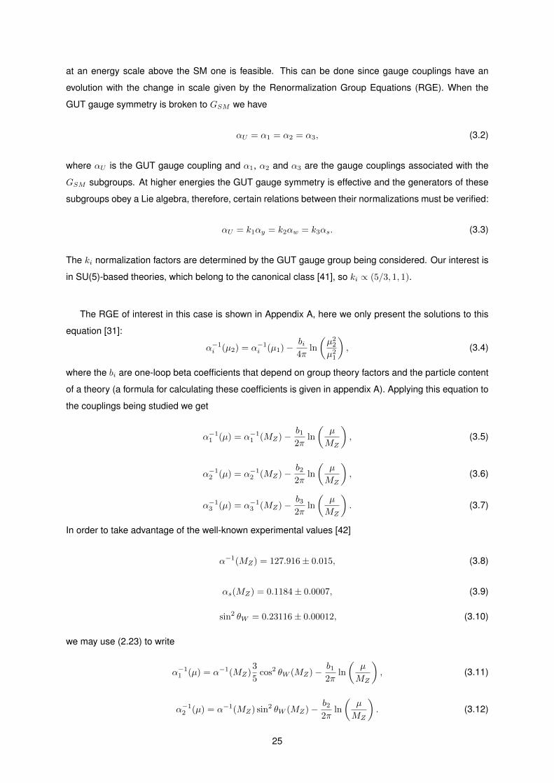
3.1 New minimal SU(5) fields that contribute to the B-test and their influence. . . . . . . . . . 32

3.2 Contributions to the B-test from 45H fields. . . . . . . . . . . . . . . . . . . . . . . . . . . . 35

4.1 Sufficient conditions for proton decay suppression in the T1 mediated case. . . . . . . . . 47

4.2 Sufficient conditions for proton decay suppression in the T2 mediated case. . . . . . . . . 48

4.3 Sufficient conditions for proton decay suppression in the ∆−1/3 mediated case. . . . . . . 49

4.4 Sufficient conditions for proton decay suppression in the ∆2/3 mediated case. . . . . . . . 49

4.5 The first column indicates the number of Mu zeros and the first row indicates the number

of Md zeros. . . . . . . . . . . . . . . . . . . . . . . . . . . . . . . . . . . . . . . . . . . . . 50

4.6 The first column indicates the number of Mu zeros and the first row indicates the number

of Md zeros. . . . . . . . . . . . . . . . . . . . . . . . . . . . . . . . . . . . . . . . . . . . . 50

5.1 Relevant contributions to the B-test in the Adjoint SU(5)× ZN model. . . . . . . . . . . . 56

xiii

xiv

List of Figures

2.1 Scalar potential with µ2 > 0 (left) and µ2 < 0 (right) . . . . . . . . . . . . . . . . . . . . . . 7

2.2 Lowest order contributions to Tµνλ. . . . . . . . . . . . . . . . . . . . . . . . . . . . . . . . 15

2.3 Lowest order contributions to Tµν . . . . . . . . . . . . . . . . . . . . . . . . . . . . . . . . 16

2.4 Triangle diagrams with vertices vector-vector-axial for non-Abelian gauges. . . . . . . . . 19

3.1 SM gauge couplings running. . . . . . . . . . . . . . . . . . . . . . . . . . . . . . . . . . . 26

3.2 Diagram associated with th d=5 Weinberg operator. . . . . . . . . . . . . . . . . . . . . . 36

3.3 Feynman diagram representing the exchange of heavy particles that generates type I

seesaw. . . . . . . . . . . . . . . . . . . . . . . . . . . . . . . . . . . . . . . . . . . . . . . 37

3.4 Feynman diagram representing the exchange of heavy particles that generates type II

seesaw. . . . . . . . . . . . . . . . . . . . . . . . . . . . . . . . . . . . . . . . . . . . . . . 39

3.5 Feynman diagram representing the exchange of heavy particles that generates type III

seesaw. . . . . . . . . . . . . . . . . . . . . . . . . . . . . . . . . . . . . . . . . . . . . . . 40

4.1 Diagrams associated with T1 mediated proton decay. Some diagrams represent several

processes as Q and L can correspond to different particles. . . . . . . . . . . . . . . . . . 47

4.2 Diagrams associated with T2 mediated proton decay. . . . . . . . . . . . . . . . . . . . . . 48

4.3 Diagrams associated with ∆−1/3 mediated proton decay. . . . . . . . . . . . . . . . . . . . 48

4.4 Diagrams associated with ∆2/3 mediated proton decay. . . . . . . . . . . . . . . . . . . . 49

5.1 Correlation plots involving VCKM moduli, specifically, Vub vs. Vcb. The red dots represent

this work’s results, the blue ones represent all the possibilities. . . . . . . . . . . . . . . . 61

5.2 Correlation plots involving VCKM moduli, specifically, Vus vs. Vcb. The red dots represent

this work’s results, the blue ones represent all the possibilities. . . . . . . . . . . . . . . . 61

5.3 Correlation plots involving VCKM moduli, specifically, Vus vs. Vub. The red dots represent

this work’s results, the blue ones represent all the possibilities. . . . . . . . . . . . . . . . 62

5.4 Correlation plots involving VCKM angles, specifically, γ vs. sin 2β . The red dots represent

this work’s results, the blue ones represent all the possibilities. . . . . . . . . . . . . . . . 62

5.5 Correlation plots involving VCKM angles, specifically, J vs. sin 2β. The red dots represent

this work’s results, the blue ones represent all the possibilities. . . . . . . . . . . . . . . . 63

xv

xvi

List of Acronyms

CKM Cabibbo-Kobayashi-Maskawa

GUT Grand Unified Theory

PMNS Pontecorvo-Maki-Nakagawa-Sakata

QFT Quantum Field Theory

RGE Renormalization Group Equations

SM Standard Model

SSB Spontaneous Symmetry Breaking

vev Vacuum Expectation Value

xvii

xviii

Chapter 1

Introduction

In the beginning of the 20th century there were two paradigm shifts in Physics, Quantum Mechanics and

Relativity. Amidst the many new discoveries made at this time, it was found that electromagnetic interac-

tions are very accurately described by a relativistic Quantum Field Theory (QFT), specifically, Quantum

Electrodynamics [1]. This theory’s Lagrangian is invariant under local transformations belonging to an

Abelian group, so it is also a gauge theory. In 1954, Chen Ning Yang and Robert Mills [2] generalized

this to non-Abelian groups while trying to explain strong interactions and, for this reason, gauge theo-

ries seeking to describe elementary particle interactions using any compact, semi-simple Lie group are

known as Yang-Mills theories.

These theories were, however, abandoned at an initial stage, because the gauge symmetry would

not allow fermion and gauge boson masses, which was contrary to experimental data. In 1964, Pe-

ter Higgs [3], Robert Brout and Francois Englert [4] and Tom Kibble, Gerald Guralnik and C. R. Ha-

gen [5] proposed, independently, a mechanism involving spontaneous symmetry breaking in the context

of gauge theories that would lead to mass terms for certain particle fields. The result became known as

the Higgs mechanism and it requires a scalar particle that acquires a vacuum expectation value. Using

this procedure, Weinberg and Salam published papers, in 1967 [6] and 1968 [7], respectively, in which

they unified electromagnetic and weak interactions in a Yang-Mills theory, first suggested by Sheldon

Glashow in 1961 [8], where the differences between these interactions were attributed to a spontaneous

breakdown of gauge symmetry. Since not much was known about the renormalizability of this theory it

did not attract much attention until some important results were later proved.

These results involve the quantization and renormalization of gauge theories. Regarding the first

aspect, significant progress was achieved by scientists like Feynman, DeWit, Mandelstam, Fadeev and

Popov. As for the second aspect, detailed studies of the simplest field theory with spontaneous symme-

try breaking revealed that this phenomenon does not affect the divergences of the theory and in 1971 G.

’t Hooft [9] demonstrated that Yang-Mills theories with spontaneous symmetry breaking are renormal-

izable. All these advances enabled physicists to obtain a renormalizable Yang-Mills theory describing

strong, weak and electromagnetic interactions in 1973-74 after the strong interactions were added to

Weinberg and Salam’s electroweak model.

1

The resulting theory is known as the Standard Model of Particle Physics (SM) and it had some re-

markable successes, including the prediction of gauge bosons, that were first detected in 1979 [10]

(namely the gluons, mediators of strong interactions). This added legitimacy to the SM and gauge the-

ories in general, as did the later (1983) discovery of W and Z bosons [11–13]. When we also take

into account the remarkable quality in describing elementary interactions (gravity is not being consid-

ered)and the recent detection of Higgs bosons [14, 15]), it is clear that the SM is one of the greatest

achievements in Physics. Despite this, we know that the SM is neither a complete nor definitive theory

since it possesses certain insufficiencies such as no quantization of gravitational interactions, absence

of neutrino masses, no viable candidate for dark matter, no quantization of the electric charge and hi-

erarchy problems. Solving these issues requires Physics beyond the SM and extensive work has been

done in this context. One class of theories attempting to provide a better explanation of elementary

interactions are the Grand Unified Theories, that have electric charge quantization as the main motiva-

tion, as aspects like the cancellation of proton and electron electric charges are very important for the

existence of the macroscopic world as we know it. This is achieved by having a gauge group larger than

the SM one that is also simple or a direct product of identical simple groups while embedding the SM

group and it undergoes spontaneous symmetry breaking in such a way that this last group is returned

in the low-energy limit. A relevant consequence is that the SM’s three gauge couplings (one for every

type of interaction) are replaced by a single one that is observed above a certain energy scale and is

split into the three SM couplings at low-energy scales after spontaneous symmetry breaking (hence the

name of this kind of theories).

The simplest GUTs are based on the SU(5) group and the simplest of these models is called minimal

SU(5). It was introduced in 1974 by Howard Georgi and Sheldon Glashow [16], having the merit of

providing electric charge quantization from theoretical aspects, but many other problems remain while

new ones, like proton decay and wrong mass predictions, arise. This may not seem very promising,

however, the runing of SM gauge couplings, which almost unify at a certain scale, the aforementioned

accomplishments and the fact that most of these issues can be solved without radically changing the

theory make SU(5) GUTs a well-motivated framework and a good starting point for building a flavour

symmetry. Many models may be obtained by altering the minimal scenario and the background for this

thesis is one of these, the Adjoint-SU(5) [17]. Its advantages and disadvantages will be debated later

but the main focus is on proton decay. In fact, this problem affects GUTs in general as they imply the

existence of new fields that can mediate these decays but no such event has been detected thus far

and, as a consequence, the new fields in question have their masses strongly constrained. Therefore,

it is of interest to study possibilities of eliminating this issue. One interesting way of doing so is by

means of adding discrete symmetries to the gauge group and the main purpose of this thesis is to study

the symmetries that may successfully be used and weather the models obtained are consistent with

experimental data.

This work starts with a brief review of the Standard Model of Particle Physics, especially of its elec-

troweak sector as it contains the phenomenology that is more relevant for the rest of the thesis. Gauge

anomalies are also mentioned as they spoil a theory’s renormalizability and must, therefore, be absent

2

in any realistic model. Chapter 3 is dedicated to Grand Unified Theories and their general features are

introduced in a discussion of the minimal SU(5) model. This discussion reveals that the minimal setup

has a considerable number of problems so several pertinent extensions are presented to address them.

Of particular importance are the see-saw mechanisms that allow neutrinos to acquire mass. In Chapter

4 the Adjoint model is introduced and we study the proton decay processes that may take place in this

context. A discrete symmetry is introduced with the purpose of loosening constraints related to this

issue while reducing the arbitrariness in the Yukawa sector. In Chapter 5 we attempt to build realistic

theories without tree-level scalar-mediated proton decays by choosing particular discrete symmetries

and associated charges. Finally, this work’s conclusions are summarized in Chapter 6.

3

4

Chapter 2

The Standard Model of Particle

Physics

The SM is, without a doubt, an important milestone in particle physics. In spite of its shortcomings, it

gives a very good description of low-energy interactions, which is why many models of greater complexity

return it (with a few possible changes) as an effective theory in this limit. Besides, some of its main

”ingredients”, such as a gauge group and the Higgs mechanism are present in a wide variety of more

sophisticated gauge theories, so it is very important to understand them. In this Chapter we go over

some of the SM’s main features, with emphasis on the electroweak sector. Afterwards, we make a

simplified analysis of gauge anomalies in order find out which conditions must be verified for them to be

absent and prove that the SM is anomaly-free.

2.1 Gauge group and Higgs mechanism

The Standard Model is a relativistic Quantum Field Theory. As happens with this kind of theories, be

they classical or quantum in nature, the main quantity is the Lagrangian L, from which we can obtain the

field’s equations of motion by applying the principle of stationary action:

δS = δ

∫d4xL = 0⇔

∫d4x

[∂L∂φi

δφi +∂L

∂(∂µφi)δ(∂µφi)

]=

∫d4x

[∂L∂φi− ∂µ

∂L∂(∂µφi)

]δφi

⇒ ∂L∂φi− ∂µ

∂L∂(∂µφi)

= 0.

(2.1)

These are known as the Euler-Lagrange equations.

More specifically, the SM is a gauge theory, which means that its Lagrangian is invariant for a certain

group of local transformations. That group is

GSM = SU(3)C × SU(2)L × U(1)Y (2.2)

where SU(3)C is associated with strong interactions, SU(2)L is associated with weak interactions and

5

U(1)Y is the hypercharge group. Local transformations have an explicit dependence on the space-

time coordinates so terms with gradients are not invariant. For a non-Abelian group (like groups from

the SU(n) family) this problem can be solved by adding vector bosons to the theory and replacing the

gradients with covariant derivatives using the following prescription (minimal coupling) [18]∂µ → Dµ =

∂µ − igL.Aµ(x). In the previous equation, g is the coupling constant, Li are matrix representations of

the group generators and Aiµ(x) are the vector boson fields. This is easily generalized to Abelian cases

by replacing the Li with a constant. It is important to note that one vector boson is added for every

generator of the gauge group.

From this procedure of minimal coupling and (2.2) we can see that, in the SM, covariant derivatives

may be written as

Dµ = ∂µ − igS8∑a=1

Gaµλa

2− ig

3∑a=1

W aµ

σa

2− igY

Y

2Bµ, (2.3)

where the second term on the right corresponds to the SU(3)C group, whose generators are represented

by the λa Gell-Mann matrices (shown in Appendix B), the third term corresponds to the SU(2)L group,

whose generators are represented by the σa Pauli matrices and the last term corresponds to U(1)Y ,

represented by the constant Y. There are 12 vector bosons, 8 Gaµ, 3 W aµ and Bµ.

The interactions between gauge bosons and other fields are given by the kinetic terms of the other

fields, with partial derivatives replaced by covariant ones. It is still necessary to add the kinetic terms

for the gauge bosons (terms that only include these fields or their derivatives). In the Abelian case the

field-strength tensor is defined as

Fµν = ∂µAν − ∂νAµ (2.4)

and the gauge-kinetic term to be added to the Lagrangian is

− 1

4FµνFµν . (2.5)

In the non-Abelian case the field-strength tensor is

F aµν = ∂µAaν − ∂nuAaµ − gfabcAbµAnuc, (2.6)

where fabc are the structure constants of the group (for a definition of structure constants and a review

of Lie Algebras see [19]). The gauge-kinetic term has the same form as (2.5). Considering this, the

terms that must be added to the SM Lagrangian are

Lgauge−kinetic = −1

4BµνBµν −

1

4W aµνW a

µν −1

4GaµνGaµν . (2.7)

At this point we note that mass terms for the gauge bosons of the form

m2AµAµ (2.8)

would explicitly break the gauge symmetry. It has been experimentally observed that some of these

6

bosons have mass, namely, the ones associated with weak interactions, and it is known that the cor-

responding isospin symmetry is broken. We could consider explicitly breaking the symmetry by adding

these mass terms, but the gauge boson masses would be arbitrary parameters of the model. Instead,

we look for another way of breaking the symmetry that offers more predictivity, namely, Spontaneous

Symmetry Breaking. Furthermore, if we choose the path of explicit symmetry breaking, certain Feyn-

man diagrams have ”worse” divergences than in the case with Spontaneous Symmetry Breaking and, in

that context, unitarity is lost, while renormalizability itself would, in general, also be lost [20].

How can a symmetry be broken in a non-explicit way and how can the bosons related to the broken

symmetry acquire mass in that scenario? The answer is provided by the so-called Higgs mechanism [3–

5]. A scalar field φ is postulated to exist. This field is an SU(2)L doublet that can be written as

φ =

φ+

φ0

. (2.9)

The most general renormalizable potential for φ is

V (φ†φ) = µ2(φ†φ) + λ(φ†φ)2, (2.10)

where µ and λ are constants. If λ < 0 the field oscillations are unbounded so λ is taken to be positive.

On the other hand, µ2 can be positive or negative. When it is considered that µ2 > 0, the minimum of

the potential is 0 with 〈φ〉0 = 0. When µ2 is considered to be negative the potential changes and its

minimum is no longer 0, as shown in Figure 2.1. The minimum occurs for 〈φ〉0 = −µ2

λ = v2 now, where

v is a real and positive constant. From this point on only the case with µ2 < 0 is considered for reasons

that will become clear soon.

Figure 2.1: Scalar potential with µ2 > 0 (left) and µ2 < 0 (right)

Taking advantage of the freedom to perform SU(2)L rotations the vacuum state of φ can be parametrized

as

〈φ〉0 =1√2

0

v

. (2.11)

Contrarily to the case where 〈φ〉0=0, this vacuum does not preserve the SU(2)L×U(1)Y gauge symmetry

since

eiαk〈φ〉0 ≈ (1 + iαk)〈φ〉0 6= 〈φ〉0, (2.12)

7

where the k indexes refer to SU(2)L × U(1)Y generators. This means that, in general, electroweak

gauge group transformations don’t leave the vacuum invariant and, consequently, there is a symmetry

breaking. This phenomenon is usually referred to as Spontaneous Symmetry Breaking (SSB) because

the Lagrangian itself has a certain gauge symmetry but the physical system as a whole does not. There

is still an U(1) subgroup of the electroweak gauge group under which the theory is invariant. Defining

Q =σ3

2+ Y (2.13)

and assigning φ an hypercharge of 12 the result of acting with Q upon the vacuum of the scalar field is

Q〈φ〉0 =

1 0

0 0

0

v

=

0

0

. (2.14)

This Q leaves the vacuum invariant and it is the generator of the residual U(1) gauge group.

From the previous discussion one can see that 3 of the 4 generators of the electroweak gauge group

are broken so, according to Goldstone’s Theorem [21], there should be 3 massless Goldstone bosons

in the theory. At this point, two problems arise when comparing the theory described so far with experi-

mental results: no Goldstone bosons have been observed and three gauge bosons are massive. These

issues are related and have a common explanation, the so-called Higgs mechanism. The fact that the

Lagrangian has gauge invariance allows one to make certain local transformations without changing the

physics of the model. It is possible, using one of those transformations, to make the Goldstone bosons

”disappear”. These bosons are ”gauged away” and the gauge in which this happens is called unitary

gauge. Being more rigorous, the Goldstone bosons do not completely vanish, they are incorporated as

degrees of freedom of gauge boson fields that, as a consequence, become massive [18].

It has already been stated that mass terms for the gauge bosons can’t be included in the gauge-

kinetic part of the Lagrangian. Instead, they arise from the kinetic term of the Higgs field. This field, in

the unitary gauge, can be parametrized as

φ =

0

(v +H)/√

2

, (2.15)

where H is a real scalar field. Looking at the scalar potential in (2.10) we note, using (2.15), that there

are small oscillations around the vev which correspond to a boson with a mass of

m2H = −2µ2 = 2v2λ. (2.16)

With this parametrization the kinetic term of φ is

(Dµφ)†(Dµφ) =1

2∂µH∂

µH + g2 (v +H)2

4

1√2

(A1µ + iA2

µ)1√2

(A1µ − iA2µ)

+(v +H)2

8(g2A3

µA3µ − ggYA3

µBµ − ggYA3

µBµ − g2

YBµBµ).

(2.17)

8

The A1µ, A2

µ, A3µ and Bµ fields are not mass eigenstates so they are not physical fields. It is, then, useful

to introduce new fields that are mass eigenstates. Regarding the second term on the right-hand side of

(2.17), the new fields are defined as

W±µ =A1µ ∓ iA2

µ√2

(2.18)

and this term becomes

g2 v2

4W−µ W

+µ, (2.19)

from which it can be seen that the new fields have a mass of

MW =

√1

4g2v2 =

1

2gv. (2.20)

Ignoring the H field (because at this point the focus is on the boson masses), the third term on the right

of (2.17) may be written as

v2

8(A3

µBµ)

g2 −ggY−ggY g2

Y

A3µ

Bµ

. (2.21)

Finding the mass eigenstates is, in this case, equivalent to diagonalizing the mass matrix in the previous

equation. This is done by defining the new fields as the ones that give the old fields when rotated by a

certain angle (Weinberg angle):A3µ

Bµ

=

cos θW sin θW

− sin θW cos θW

ZµAµ

, (2.22)

with

cos θW =g√

g2 + g2Y

, sin θW =gY√g2 + g2

Y

. (2.23)

Using (2.22) in (2.21) the mass term becomes

v2

8(ZµAµ)

g2 + g2Y 0

0 0

ZµAµ

, (2.24)

from which it can be seen that Zµ has a mass of MZ = v2

√g2 + g2

Y and Aµ has no mass. The boson

associated with electroweak interactions that remains massless after SSB is the photon so Aµ is iden-

tified as this field [22]. Breaking the gauge symmetry through SSB we have obtained all gauge boson

masses in terms of other parameters of the model.

It is convenient to rewrite the covariant derivative given by (2.3) in terms of the physical fields. Defin-

ing

T± =σ1/2± iσ2/2√

2(2.25)

one gets:

Dµ = ∂µ − ig√2

(W+µ T

+ +W−µ T−)− i 1√

g2g2Y

Zµ(g2σ3/2− g2Y Y )− i ggY√

g2 + g2Y

Aµ(σ3/2 + Y ). (2.26)

9

The last term involves the photon, therefore, it corresponds to the electromagnetic interaction. Knowing

this, one can conclude thatggY√g2 + g2

Y

= g sin θW = e (2.27)

and σ3/2 + Y gives the electric charge. The previously defined Q is, then, the electric charge operator

and the U(1) gauge group it generates corresponds to electromagnetism. This gauge symmetry is not

broken in the SM and the electric charge is conserved, in accordance with all experimental data collected

so far. Making appropriate substitutions, (2.26) can be written as

Dµ = ∂µ − ig√2

(W+µ T

+ +W−µ T−)− i g

cos θWZµ

(σ3

2− sin2 θWQ

)− ieAµQ. (2.28)

2.2 Fermion masses and Mixings

Other than the gauge bosons and Higgs fields, the SM also includes another type of particles, elemen-

tary fermions. These are Dirac particles with a spin of 1/2 and form most of the matter we see around

us (most of the bound states found in nature are constituted by them). Fermions can be classified as

quarks, which experience all four fundamental interactions in nature, or leptons, that don’t have strong

interactions. These particles, in the SM, appear as left-handed or right-handed fields where

ΨL =1− γ5

2Ψ, ΨR =

1 + γ5

2Ψ. (2.29)

The left-handed components are SU(2)L doublets while the right-handed ones are singlets under this

group. Regarding the SU(3)C group, quarks form triplets while the leptons are singlets, as one would

expect given the fact that they don’t experience strong interactions. Finally, the hypercharge quantum

numbers are assigned in order to get the correct (experimentally observed) electric charge for the fields

from (2.14). The quantum number of the fermion fields in relation to GSM are displayed in Table 1.

Quark Fields Quantum Numbers Lepton Fields Quantum Numbers

qL =

(uLdL

)(3,2,1/6) LL =

(νe−

)(1,2,−1/2)

uR (3,1,2/3) eR (1,1,−1)

dR (3,1,−1/3)

Table 2.1: SM fermions and their GSM quantum numbers.

10

It is known that fermions are massive but mass terms like

LFermionMass = −m(ψRψL + ψLψR) (2.30)

cannot be added to the Lagrangian because they would explicitly break the electroweak gauge symme-

try. This is due to the fact that right-handed and left-handed fields belong to different representations of

the electroweak gauge group. There must be some other way for the fermions to acquire mass in the

SM.

Using the scalar field φ it is possible to obtain SU(2)L ×U(1)Y -invariant terms that mix right-handed

and left-handed fermion fields:

LYukawa = −QiLY uij φujR − Q

iLY

dijφd

jR − L

iLY

eijφe

jR +H.c., (2.31)

where φ = iσ2φ∗ and the Y u,d,e are arbitrary complex 3 × 3 Yukawa matrices. When φ gets a vev of v

there is SSB and the following mass terms arise from the previous equation:

LMass = −uiLM iju u

jR − d

iLM

ijd d

jR − e

iLM

ije e

jR +H.c.. (2.32)

The fermion mass matrices, Mu, Md and Me are given by

Mu =1√2vY u, Md =

1√2vY d, Me =

1√2vY e. (2.33)

It should be noted that, since there are no right-handed neutrino fields in the SM, these particles do not

acquire mass in this way.

Since the Yukawa matrices are not, in general, diagonal, the fermion eigenstates of the electroweak

interactions are not mass eigenstates. These last eigenstates are obtained by diagonalizing the mass

matrices using the following bi-unitary transformations:

uL = UuLu′L, uR = UuRu

′R, (2.34)

dL = UdLd′L, dR = UdRd

′R, (2.35)

eL = UeLe′L, eR = UeRe

′R, (2.36)

νL = UeLν′L, (2.37)

where the Us are unitary matrices and the primed fields are the physical fields (mass eigenstates). After

these transformations are performed the masses become

Uu†L MuUuR = diag(mu,mc,mt) = Du, (2.38)

Ud†L MdUdR = diag(md,ms,mb) = Dd, (2.39)

11

Ue†L MeUeR = diag(me,mµ,mτ ) = De. (2.40)

It should be stated that the m values represent actual masses so they are real and positive.

Due to the arbitrariness of the Yukawa matrices, UuL is different from UdL and this leads to mixings

between quarks. To see how this happens it is convenient to analyse the interactions of fermions with

the gauge bosons. These interactions are given by the Dirac Lagrangian with the partial derivatives

replaced by covariant ones:

LInteractions = g(W+µ J

µ+W +W−µ J

µ−W + ZµJ

µZ) + eAµJ

µEM , (2.41)

where the J’s are currents that may be written as

Jµ+W =

1√2

(uLγµdL + νLγ

µeL), Jµ−W =1√2

(dLγµuL + eLγ

µνL), (2.42)

JµZ =1

cos θW

[uLγ

µ(1

2− 2

3sin2 θW )uL + uRγ

µ(−2

3sin2 θW )uR + dLγ

µ(−1

2+

1

3sin2 θW )dL+

+ dRγµ(

1

3sin2 θW )dR + νLγ

µ 1

2νL + eLγ

µ(−1

2+ sin2 θW )eL + eRγ

µ sin2 θW eR

],

(2.43)

JµEM =2

3uγµu− 1

3dγµd− eγµe. (2.44)

When fermions fields are rotated to the mass eigenstate basis, the left-handed components of the quarks

get mixed, as one can see in the positive charged weak current:

Jµ+W =

1√2

(u′LγµUu†L UdLd

′L + ν′Lγ

µUe†L UeLe′L). (2.45)

While Ue†L UeL is the identity and no mixing occurs on the lepton sector, Uu†L UdL = V is different form the

identity, it is a complex 3× 3 unitary matrix known as the CKM matrix [23,24], that may be written as

V =

Vud Vus Vub

Vcd Vcs Vcb

Vtd Vts Vtb

. (2.46)

Note that, since neutrinos are massless in the SM, we can change their basis using the same unitary

matrix as we do for left-handed charged leptons and, consequently, no lepton mixing occurs.

Some parameters of the VCKM are devoid of physical meaning, as we are free to rephase quark

fields through

uα = eiΨαu′α

dk = eiΨkd′k,(2.47)

where the Ψ are arbitrary phases. These transformations lead to

V ′αk = ei(Ψk−Ψα)Vαk (2.48)

12

and, with ng fermion generations, we can use this to eliminate 2ng−1 VCKM phases [25]. Usually, being

unitary, this matrix would contain n2g parameters but, considering the previous discussion, this number

becomes

Nparam = n2g − (2ng − 1) = (ng − 1)2. (2.49)

Out of these,

Nangle =1

2ng(ng − 1) (2.50)

may be identified as rotation (Euler) angles. The remaining

Nphase = Nparam −Nangle =1

2(ng − 1)(ng − 2) (2.51)

parameters correspond to physical phases. For ng = 3 we see that there is only one such phase

and it can be shown that this phase leads to CP violation [25]. The phenomenon of CP violation is

very interesting as it can provide (along with the assumption of departure from thermal equilibrium

and non-conservation of baryon number) an explanation for the baryon asymmetry in the observable

universe [26], but the CP violation predicted in the SM is not sufficient [27]. We could consider this a

problem, however, there are other possible sources of baryon asymmetry so we dismiss this issue and

CP violation will not be studied in the remaining chapters.

Later in this work we will want to compare the predicted VCKM with experimental results related to

quark mixings, so it is of interest to define rephasing-invariant quantities that may be measured through

appropriate experiments. The simplest possibility is given by

Uαi ≡ |Vαi|2, (2.52)

the moduli of the matrix elements. Another one is provided by invariant quartets, defined as

Qαiβj ≡ VαiVβjV ∗αjV ∗βi, (2.53)

where α 6= β and i 6= j. Since the VCKM matrix is unitary, its rows and columns must verify orthogonality

conditions. Considering, for example, the first and third columns we have

VudV∗ud + VcdV

∗cb + VtdV

∗tb = 0. (2.54)

We may interpret this equation as a triangle in the complex plane and, while rephasing of the quark fields

rotates the triangle, all internal angles and length of its sides remain invariant. Choosing a convention in

which VcdV ∗cb is real and negative, the inner angles of the triangle are defined by

α ≡ arg(−Qubtd),

β ≡ arg(−Qtbcd),

δ ≡ arg(−Qcbud).

(2.55)

13

The moduli in (2.52) and the α, β and δ are well measured physical quantities and we will use them

to test weather or not our predicted VCKM is consistent with experimental data. Note also that, by

definition, α+ β + γ = π mod 2π

2.3 Gauge Anomalies

The Lagrangian function plays an important role in the SM and QTF’s in general but, unlike what hap-

pens in classical theories, one must consider corrections to the interactions given by this function and

even possible non-perturbative effects beyond the Lagrangian (these latter are not relevant in the context

of this work). Radiative corrections are mentioned here because they can have important consequences

for the theory, such as violating symmetries of the underlying Lagrangian and jeopardizing its renormal-

izability.

In classical theories there is a correspondence between symmetries of the Lagrangian and con-

served charges given by Noether’s theorem. As for quantum field theories, the symmetry properties of

the Lagrangian lead to relations between Green’s functions, which are known as Ward Identities [28].

These identities have several applications but in this context the focus will be on their role in the renor-

malization programme of any theory with nontrivial symmetries. If the identities are violated by radiative

corrections then it is impossible to prove the renormalizability of the theory [9]. A particular case of

this will be analysed in this section, specifically the Adler-Bell-Jackiw anomaly [29, 30], named after the

researchers that discovered it in 1969-1970.

To begin with, currents may be classified according to their transformation properties as scalar (S),

vector (V), tensor (T), pseudoscalar (P) or axial vector (A):

S(x) = Ψ(x)Ψ(x), (2.56)

Vµ(x) = Ψ(x)γµΨ(x), (2.57)

Tµν(x) = Ψ(x)γµγνΨ(x), (2.58)

P (x) = Ψ(x)γ5Ψ(x), (2.59)

Aµ(x) = Ψ(x)γµγ5Ψ(x). (2.60)

Considering the following three-point functions of electrodynamics,

Tµνλ(k1, k2, q) = i

∫d4x1d

4x2 〈0 | T (Vµ(x1)Vν(x2)Aλ(0)) | 0〉 eik1·x1+ik2·x2 (2.61)

and

Tµν(k1, k2, q) = i

∫d4x1d

4x2 〈0 | T (Vµ(x1)Vν(x2)P (0)) | 0〉 eik1·x1+ik2·x2 , (2.62)

where q = k1 + k2, one may obtain the Ward identities relating Tµνλ and Tµν to check weather they are

14

verified. Using the divergences of Vµ and Aµ, which are calculated from the equation of motion

∂µVµ(x) = 0 (2.63)

∂µAµ(x) = 2imP (x), (2.64)

where m is the mass of Ψ, current-algebra techniques like

∂µx (T (Jµ(x)O(y))) = T (∂µJµ(x)O(y)) + [J0(x), O(y)] δ(x0 − y0) (2.65)

and with the knowledge that

[V0(x), A0(y)] δ(x0 − y0) = 0, (2.66)

we get the following vector and axial-vector Ward Identities [31]

kµaTµνλ = kνb Tµνλ = 0, (2.67)

qλTµνλ = 2mTµν . (2.68)

Figure 2.2: Lowest order contributions to Tµνλ.

The lowest order contributions to Tµνλ and Tµν come from the diagrams shown in Figures 2.2 and

2.3, respectively, and may be written as

Tµνλ = i

∫d4p

(2π)4(−1)

Tr

[i

�p−mγλγ5

i

(�p− �q)−mγν

i

(�p− �k1)−mγµ

]+

k1 ↔ k2

µ↔ ν

; (2.69)

Tµν = i

∫d4p

(2π)4(−1)

Tr

[i

�p−mγ5

i

(�p− �q)−mγν

i

(�p− �k1)−mγµ

]+

k1 ↔ k2

µ↔ ν

. (2.70)

Using

�qγ5 = γ5(�p− �q −m) + (�p−m)γ5 + 2mγ5 (2.71)

15

Figure 2.3: Lowest order contributions to Tµν .

we can obtain

qλTµνλ = 2mTµν + ∆(1)µν + ∆(2)

µν , (2.72)

with

∆(1)µν =

∫d4p

(2π)4Tr

{i

�p−mγ5γν

i

(�p− �k1)−mγµ −

i

(�p− �k2)−mγ5γν

i

(�p− �q)−mγµ

}(2.73)

and

∆(2)µν =

∫d4p

(2π)4Tr

{i

�p−mγ5γν

i

(�p− �k2)−mγµ −

i

(�p− �k1)−mγ5γν

i

(�p− �q)−mγµ

}. (2.74)

One can readily see that the Ward Identity in (2.68) is only respected if ∆(1)µν + ∆

(2)µν = 0. The two

integrals in (2.73) would cancel each other if one could make the shift p → p + k2 in the second term

inside the trace. Applying the same reasoning to (2.74) and performing the shift p→ p+k1 in the second

term inside the trace we see that this expression would also vanish. However, this procedure can only

be applied to convergent integrals, which constitutes a problem since these ∆s are linearly divergent.

Before studying the conditions in which (2.68) can be valid it is important to clarify this last point.

Starting with the one-dimension case it is easy to show that a shift of integration variable may be

impossible if the integral is divergent [32]. For an integration variable shift to be legitimate the quantity

given by

∆(a) =

∫ +∞

−∞dx [f(x+ a)− f(x)] (2.75)

must vanish. Expanding the integrand and taking into account the fact that, for linearly divergent inte-

grals, f(±∞) 6= 0, one gets

∆(a) = a [f(∞)− f(−∞)] , (2.76)

a surface term that is, in general, different from 0.

Generalizing (2.75) to an n−dimensional space, expanding the integrand, integrating over the surface

r = R →∞ and applying Gauss’s theorem, one can see that only the first term of the expansion, given

16

by

∆(a) = aτRτRf(R)Sn(R) (2.77)

remains, where RτR is the outward pointing unit normal field and Sn(R) is the surface area of the hyper-

sphere with radius R. In the four-dimensional Minkowski space, S3(R) = 2π2R3 so we get

∆(a) = aτ∫d4r∂τf(r) = 2iπ2aτ limR→∞R

2Rτf(r). (2.78)

The fact that Tµνλ is linearly divergent implies that this quantity is not uniquely defined. In (2.69)

the fermion line between the vector and axial-vector vertices carries momentum p but we may, instead,

assign it a momentum of p+ a where a is an arbitrary linear combination of k1 and k2:

a = αk1 + (α− β)k2. (2.79)

The ambiguity in the definition of Tµνλ may be measured through the difference between amplitudes in

∆µνλ = Tµνλ(a)− Tµνλ(0) =

= (−1)

∫d4p

(2π)4

{Tr

[1

(�p+ �a)−mγλγ5

1

(�p+ �a− �q)−mγν

1

(�p+ �a− �k1)−mγµ

]−

−Tr

[1

p−mγλγ5

1

(�p− �q)−mγν

1

(�p− �k1)−mγµ

]}+

k1 ↔ k2

µ↔ ν

≡≡ ∆

(1)µνλ + ∆

(2)µνλ,

(2.80)

where Tµνλ(a) is the shifted amplitude. Using (2.78) one gets

∆(1)µνλ = (−1)

∫d4p

(2π)4aτ

∂

∂pτtr

[1

�p−mγλγ5

1

(�p− �q)−mγν

1

(p− k1)−mγµ

]=

=−i2π2aτ

(2π)4limp→∞

p2pτ tr(γαγλγ5γβγνγδγµ)pαpβpδ/p6 =

=i2π2aσ(2π)4

limp→∞

pσpρ

p24iεµνλρ.

(2.81)

Considering the symmetric limit we replace pσpρ/p2 with gρσ/4 and we may write

∆(1)µνλ = ερµνλa

ρ/8π2. (2.82)

There is no need to compute ∆(2)µνλ explicitly as it only differs from ∆

(1)µνλ by the exchanges k1 ↔ k2 and

µ↔ ν. Bearing this in mind and combining (2.80), (2.82) and (2.79) we get

∆µνλ = ∆(1)µνλ + ∆

(2)µνλ =

β

8π2ερµνλ(k1 − k2)ρ, (2.83)

from which we conclude that the ambiguity in Tµνλ may be expressed in terms of the arbitrary parameter

17

β:

Tµνλ(a) = Tµνλ(0)− β

8π2εµνλρ(k1 − k2)ρ ≡ Tµνλ(β). (2.84)

A very important question arises at this point: is there a value of β for which the Ward Identities are

verified? Starting with the Axial Ward Identity (2.68), we can use (2.78) to evaluate the linearly divergent

terms in (2.72), which yields

∆(1)µν = − kτ2

(2π)4

∫d4p

∂

∂pτ(tr[(�p+m)γ5γν(�p−��k1 +m)γµ

](p2 −m2) [(p− k1)2 −m2]

) =

= − kτ2(2π)4

2iπ2 limp→∞

pτp2tr(γαγ5γνγβγµ)pαkβ1 =

=−1

8π2εµνσρk

σ1 k

ρ2

(2.85)

and

∆(2)µν = ∆(1)

µν . (2.86)

Therefore, from (2.84) and (2.72) we obtain

qλTλνλ(β) = 2mTµν(0)− 1− β4π2

εµνσρkσ1 k

ρ2 (2.87)

and it is clear that the Axial Ward Identity is verified only if β = 1.

Moving on to the Vector Ward Identity (2.67) we have

kµ1Tµνλ(0) =(−1)

∫d4p

(2π)4

{tr

[1

�p−mγλγ5

1

(�p− �q)−mγν

1

(�p−��k1)−mγµ

]+

+tr

[1

�p−mγλγ5

1

(�p− �q)−m��k1

1

(�p−��k2)−mγν

]}.

(2.88)

Using the relation

�k1 = (�p−m)−[(�p− �k1)−m

]=[(�p− �k2)−m

]− [(�p− �q)−m] (2.89)

we can write (2.88) as

kµ1Tµνλ(0) = (−1)

∫d4p

(2π)4tr

[γλγ5

1

(�p− �q)−mγν

1

(�p− �k1)−m− γλγ5

1

(�p− �k2)−mγν

1

�p−m

]. (2.90)

Like before, we can use (2.78) to evaluate the linearly divergent integrals in the previous expression,

which leads to

kµ1Tµνλ(0) =kτ1

(2π)4

∫d4p

∂

∂pτ(Tr[γλγ5(�p− �k2 +m)γν(�p+m)

][(p− k2)2 −m2] (p2 −m2)

) =

=kτ1

(2π)42iπ2 lim

p→∞

pτp2tr(γ5γλγαγνγβ)kα2 p

β =

=−1

8π2ελσνρk

ρ1kσ2 .

(2.91)

18

Finally, remembering (2.84) we get

kµ1Tµνλ(β) =(1 + β)

8π2ενλσρk

σ1 k

ρ2 . (2.92)

It is clear from this expression that the Vector Ward Identity is only verified when β = −1 and, more

importantly, the Ward Identities in (2.67) and (2.68) cannot be simultaneously respected for any value of

β. This means that at least one of the Ward Identities is violated. When a symmetry of the Lagrangian

is broken by a perturbative correction to the theory, as in the case being studied, we say we have an

anomaly.

Although it is already evident that we have an anomaly in this situation, the parameter β is still not

fixed, which constitutes a problem since it has physical consequences. Experimental results show that

the Vector Ward Identity is verified, therefore, β = −1 and the Axial Ward Identity is violated. The fact

that we were unable to obtain the value of β is related to the renormalization scheme used, which has no

physical meaning (it is just a mathematical device) and other renormalization procedures lead directly to

(2.67) being verified [33,34]. Considering, then, β = −1 the Axial Ward Identity becomes

qλTµνλ = 2mTµν −1

2π2εµνσρk

σ1 k

ρ2 (2.93)

and the axial-vector current divergence is modified to

∂λAλ(x) = 2imP (x) + (4π)−2εµνρσFµν(x)Fρσ(x). (2.94)

The anomaly studied until this point is a non-gauge Abelian chiral anomaly, so it does not threaten

renormalizability, instead it implies that some classically forbidden processes may occur.

Figure 2.4: Triangle diagrams with vertices vector-vector-axial for non-Abelian gauges.

As for gauge anomalies, they are the ones that jeopardize the renormalizability of a theory, so it is

important to study this phenomenon. We will take a look at non-Abelian gauge anomalies since we

work with non-Abelian gauge theories and generalization of the most important results to Abelian cases

is trivial. These anomalies are more complex than the ones treated thus far and a detailed analysis

19

is beyond the scope of this work. We can, however, perform certain computations to obtain a very

important result that remains valid in more accurate studies. Considering the diagrams in Fig. 2.4 with

non-Abelian vertices the amplitude in (2.69) is modified to

T abcµνλ = −i∫

d4p

(2π)4Tr

[i

�p−mγλγ5t

c i

�p− �q −mγνt

a i

�p− �k1 −mγµt

b

]+

k1 ↔ k2

µ↔ ν

a↔ b

. (2.95)

The gamma matrices commute with group generators so we can write

T abcµνλ = −i∫

d4p

(2π)4Tr

[i

�p−mγλγ5

i

�p− �q −mγν

i

�p− �k1 −mγµ

]Tr[tctatb

]+

k1 ↔ k2

µ↔ ν

a↔ b

. (2.96)

This modification in the amplitude leads to a change in the anomalous term given in (6.93):

Aabcµν =1

4π2εµναβk

α1 k

β2 Tr

[tctatb

]+

1

4π2ενµαβk

α2 k

β1 Tr

[tctbta

]=

=1

4π2εµναβk

α1 k

β2 Tr

[tctatb + tctbta

]=

=1

4π2εµναβk

α1 k

β2 Tr

[{ta, tb

}tc].

(2.97)

This was a grossly oversimplified calculation but it turns out that the anomalous terms are, in general,

proportional to Tr[{ta, tb

}tc]

[35], so, from now on, we may take the anomaly freedom condition to be

Tr[{ta, tb

}tc]

= 0. (2.98)

Using (2.98) and the facts that fermions contribute additively to anomalies, while left- and right-

handed fermions contribute with opposite signs, it is easy to check that the SM is anomaly-free. This

last aspect can be seen by noting that the charge conjugate of left-handed field is a right-handed field

and vice-versa and applying the charge conjugation operator to the generators in (2.98) we get the same

expression preceded by a minus sign. Recalling that, in the SM, the gauge group is a direct product of

three groups, the possible anomalies are associated with triangle diagrams that couple to these groups’s

gauge bosons. We can see, then, that 10 different anomalies may arise:[U(1)Y ]3, [SU(2)L]

3, [SU(3)C ]3,

[U(1)Y ]2SU(2)L, [U(1)Y ]

2SU(3)C , U(1)Y [SU(2)L]

2, U(1)Y [SU(3)C ]2, U(1)Y SU(2)LSU(3)C , [SU(2)L]

2SU(3)C

and SU(2)L [SU(3)C ]2. Starting with the Abelian anomaly, we have

[U(1)Y ]3 →

∑fL

tr [{gY YfL , gY YfL} gY YfY ]−∑fR

Tr [{gY YfR , gY YfR} gY YfR ] =

= 2g3Y

∑fL

Y 3fL −

∑fR

Y 3fR

= 2g3Y ng(6Y

3q + 2Y 3

l − 3Y 3u − 3Y 3

d − Y 3e ) = 0.

(2.99)

20

Next, using T i = σi

2 as the SU(2) generators, we obtain

[SU(2)L]3 → Tr

[{gT a, gT b

}gT c

]= g3 Tr

[1

2δabT c

]=g3

2δab Tr [T c] = 0, (2.100)

where the last equality follows from the fact that the T i are traceless. We can readily see that other pos-

sible anomalies, specifically [U(1)Y ]2SU(2)L, [U(1)Y ]

2SU(3)C , [SU(2)L]

2SU(3)C , SU(2)L [SU(3)C ]

3

and U(1)Y SU(2)LSU(3)C , vanish for the same reason (the SU(3) generators in the fundamental repre-

sentation are also traceless). Moving on to the pure SU(3)C anomaly we have

[SU(3)C ]3 → Tr

[{gSλa

2, gS

λb

2

}gSλc

2

]=g3S

2dabcnG

∑quarks

=g3S

2dabcng(2− 1− 1) = 0. (2.101)

There are only two anomalies left to investigate, U(1)Y [SU(2)L]2 and U(1)Y [SU(3)C ]

2:

U(1)Y [SU(2)L]2 → Tr

[{gT a, gT b

}gY Yf

]= g2gY Tr

[1

2δabI2Yf

]= g2gY nG

∑fL

Yf = 0 (2.102)

and

U(1)Y [SU(3)C ]2 → Tr

[{gSλa

2, gS

λb

2

}gY Yf

]= g2

SgY Tr

[1

3δabI3Yf + dabcT cYf

]=

= g2SgY ng

∑quarks

Yf = 0,(2.103)

where In is the identity matrix in n dimensions. We have shown that the SM is anomaly-free and it

should also be noted that this result does not depend on the number of generations (anomalies cancel

within each generation).

In the SM there is no attempt to describe gravitational interactions but, obviously, this can’t be the

case for a complete theory. Any possible inclusion of gravity in a gauge theory like this leads to new

anomalies related to local Lorentz transformations. In a four-dimensional Euclidean space these can

be considered SO(4) gauge transformations [36]. Due to the similarities between SO(4) and SU(2) we

conclude that only the mixed U(1)-gravity-gravity anomaly doesn’t automatically vanish [37]. Given that

all particles couple to gravity we have

U(1)-gravity-gravity→ Tr[{ggt

aSO(4), ggt

bSO(4)

}gY Yf

]= g2

ggY∑f

Yf = 0. (2.104)

Weather or not we consider a minimal extension to couple to gravity in four dimensions, the SM is an

anomaly-free theory.

21

22

Chapter 3

SU(5) based Grand Unified Theories

In this chapter, the SM’s most relevant problems and unattractive features are discussed and we will

see that Grand Unified Theories provide a favourable framework for attempts to solve some of these

issues. The GUTs that are treated in this thesis are based in an SU(5) gauge group so we study the

minimal SU(5) model as it can be considered a prototype for more complex theories introduced in later

chapters. After summarizing the minimal model’s flaws we will look at possible extensions that lead to

several improvements.

3.1 SM shortcomings and justification for GUTs

Despite its many successes and its historical importance, the SM has several insufficiencies when it

comes to describing interactions between fields in nature. Starting with a problem that has already

been mentioned in previous chapters, we note the absence of quantized gravitational interactions in

this model. In fact, this happens in all QFT as physicists have not, thus far, been able to gauge these

interactions. Until a breakthrough occurs in this area there is nothing that can be done to solve this

problem.

We move on to an issue where SM predictions are contradicted by experimental evidence: neutrino

masses. When the origin of fermion masses in the SM was explained, no Yukawa term for the neutrino

was introduced due to the absence of νR fields in the model. This was not a problem at the time the

theory was proposed because neutrinos were thought to be massless but nowadays neutrino oscillations

have been confirmed [38], which means that these particles must be massive. Even though there can

be no Dirac mass terms for the neutrinos, there is a type of mass term that only requires the existence

of one chirality state:1

2νTLC

−1MLνL +H.c., (3.1)

where C is the Dirac matrix for which Ψc ≡ CΨT and Ψc is the anti-particle of Ψ. This term is called

a Majorana mass, and it can only be gauge-invariant for fields that carry no conserved charge. Since

neutrinos are the only fermions with no electric charge it would seem like they could have Majorana

masses. They have non-zero lepton number, L, but non-perturbative effects (the so-called instanton

23

solutions) can violate individually the lepton number L and the baryon number B. Despite this, the

combination B−L remains invariant at the quantum level. This B−L symmetry prevents any dynamical

process that could generate a Majorana mass term, therefore neutrinos remain strictly massless in the

SM.

Another problem is the large number of arbitrary parameters. The scalar potential parameters are

constrained by viability and renormalization requirements while the Yukawa matrices are constrained

by experimental data but aside from that they can take a large number of values. The fact that so

many of the parameters of the theory have to be empirically observed is unsatisfactory, it would be

desirable to have a small number of physical parameters that must be measured and a series of physical

relations enabling the other parameters to be obtained from these. Furthermore, there are three fermion

generations in the SM but no explanation is provided for this, in particular, there is no a priori reason to

have the same number of lepton and quark doublets. This last aspect is vital for anomaly cancellation

so one could use this to justify the equality in the number of doublets but that is a contrived argument.

Theories with more constrained representations and Yukawa parameters provide a more favourable

framework to study the family structure and the repetition of the gauge representations. Aside from this,

it should be noted that the SM has no viable candidate for the dark matter that we know to exist in the

Universe.

A very unappealing feature of the SM is a so-called hierarchy problem related to the Higgs boson

mass. In (2.16) we did not consider radiative corrections, so this is just the ”bare” mass, not the one

measured in experiments. These corrections are of the order Λ2 where Λ is the cut-off scale. Data from

the LHC indicates that the Higgs mass is significantly lower than the cut-off scale, which means that the

radiative corrections must cancel each other almost completely. Put in another way, these corrections

must be fine-tuned in order to reproduce the empirical evidence. Although this is not necessarily a

problem, it is not natural and leads one to believe there must be some other way to get the correct Higgs

mass using physics beyond the SM.

We conclude this exposition of the SM’s shortcomings by noting that in this theory hypercharges are

assigned to the fields in order to get the correct electric charge, that is, the theory itself does not constrain

these quantum numbers. As a consequence, there is no electric charge quantization. On the other hand,

by requiring anomaly cancellation and making some additional reasonable assumptions it is possible to

obtain the hypercharges that give the correct electric charges as the only possibility [39, 40]. This,

however, is not a very satisfactory explanation, as in the case of the number of fermion doublets. More

promising solutions to this problem include the replacement of GSM with a larger group that contains the

former as a subgroup. The existence of this larger group would automatically lead to the quantization

of the electric charge and allow the correct charge of the elementary particles to be read from the

theory (instead of being put in by hand). In this scenario, since there is only one group determining the

interactions, there should only be one gauge coupling and the different couplings we observe at the SM

energy scale would be a consequence of symmetry breaking.

Theories in which there is gauge unification are called Grand Unified Theories (GUT) [16]. Before

proceeding with the discussion of GUTs we should check weather or not this idea of a unique coupling

24

at an energy scale above the SM one is feasible. This can be done since gauge couplings have an

evolution with the change in scale given by the Renormalization Group Equations (RGE). When the

GUT gauge symmetry is broken to GSM we have

αU = α1 = α2 = α3, (3.2)

where αU is the GUT gauge coupling and α1, α2 and α3 are the gauge couplings associated with the

GSM subgroups. At higher energies the GUT gauge symmetry is effective and the generators of these

subgroups obey a Lie algebra, therefore, certain relations between their normalizations must be verified:

αU = k1αy = k2αw = k3αs. (3.3)

The ki normalization factors are determined by the GUT gauge group being considered. Our interest is

in SU(5)-based theories, which belong to the canonical class [41], so ki ∝ (5/3, 1, 1).

The RGE of interest in this case is shown in Appendix A, here we only present the solutions to this

equation [31]:

α−1i (µ2) = α−1

i (µ1)− bi4π

ln

(µ2

2

µ21

), (3.4)

where the bi are one-loop beta coefficients that depend on group theory factors and the particle content

of a theory (a formula for calculating these coefficients is given in appendix A). Applying this equation to

the couplings being studied we get

α−11 (µ) = α−1

1 (MZ)− b12π

ln

(µ

MZ

), (3.5)

α−12 (µ) = α−1

2 (MZ)− b22π

ln

(µ

MZ

), (3.6)

α−13 (µ) = α−1

3 (MZ)− b32π

ln

(µ

MZ

). (3.7)

In order to take advantage of the well-known experimental values [42]

α−1(MZ) = 127.916± 0.015, (3.8)

αs(MZ) = 0.1184± 0.0007, (3.9)

sin2 θW = 0.23116± 0.00012, (3.10)

we may use (2.23) to write

α−11 (µ) = α−1(MZ)

3

5cos2 θW (MZ)− b1

2πln

(µ

MZ

), (3.11)

α−12 (µ) = α−1(MZ) sin2 θW (MZ)− b2

2πln

(µ

MZ

). (3.12)

25

Finally, we compute the SM’s beta coefficients, obtaining

b1 =41

10, b2 = −19

6, b3 = −7 (3.13)

and use these results in (3.5), (3.6) and (3.7) to make a plot of the SM gauge couplings dependence on

energy. This plot is shown in Fig. 3.1 and we can immediately observe that unification does not occur.

There is, however, no reason to give up on this goal because, as we have already seen, any theory

attempting to describe gaugeable interactions in a realistic way must include physics beyond the SM.

Also, adding to this, it can be stated that unification almost happens, so it shouldn’t be too difficult to

solve the problem in question when the particle content is enlarged as a consequence of new physics.

From Fig. and constraints related with proton decay (these will be discussed later) we can estimate the

unification scale to be between ∼ 6× 1014GeV and ∼ 1017GeV.

Figure 3.1: SM gauge couplings running.

As we want to test the possibility of unification in other contexts it is useful to introduce a tool that

can facilitate this analysis, the B-test [43]. Taking into account contributions to the beta coefficients from

new fields with masses between the electroweak and unification scales we can define an effective beta

coefficient [44]

Bi ≡ bi +∑I

bIi rI , (3.14)

where the bIi represent the contribution from particle I with mass given by MI and the rI are ratios that

determine how relevant a particle’s contribution is as a function of its mass, specifically

rI =ln(Λ/MI)

ln(Λ/MZ). (3.15)

26

Defining Bij = Bi −Bj we obtain the following B-test,

B ≡ B23

B12=

sin2 θW − αα3

35 −

85 sin2 θW

, (3.16)

as well as the GUT scale relation

B12 ln

(Λ

MZ

)=

2π

5α(3− 8 sin2 θW ). (3.17)

The equation in (3.16) makes it easier to test unification because, while the left-hand side depends

on the particle content of the theory, the right-hand side depends only on group theory factors and

quantities that are measured at low energies, so its value is fixed once we pick a particular class of GUT

to work with. We conclude that, in an SU(5) framework, unification requires

B = 0.718± 0.003, (3.18)

while in the SM we have B ' 0.53, which means that we have to increase the value of B.

3.2 Minimal SU(5)

We begin this section by explaining the choice of SU(5). To meet the criteria of providing a GUT, a

gauge group must be simple or a direct product of identical simple groups so that the gauge coupling

is unique. On the other hand, this group should coincide with GSM at low energies, which can happen

only if it embeds the SM group. The couplings are unified when the larger (GUT) group is effective but

as the energy scale gets lower spontaneous symmetry breaking occurs and the remaining gauge group

will be GSM . Since this group has rank 4 (4 generators that can be simultaneously diagonalized), any

GUT gauge group must have rank 4 or higher. There are many possibilities for which these conditions

are met but we are not looking for a radically different theory; the best course of action is to consider the

simplest candidates.

In this context, the SU(5) gauge group constitutes a favourable choice. It contains GSM and has the

same rank as it, while also having a minimal particle content, that is, among all possible GUTs based on

rank 4 groups it is the one in which the number of fields that have to be added to the SM particle content

is smallest. In this section we will study the minimal SU(5) model, which, as the name indicates, is a

minimal extension of the SM into a GUT. As will later be seen, this model has many flaws and is clearly

not correct but it serves as a basis on which more sophisticated SU(5) GUTs can be built.

According to what was already said, there is a spontaneous symmetry breaking form SU(5) to GSM

and from this last group to SU(3)C × U(1)Q. For reasons that will be explained later, the new gauge

bosons implied by the larger gauge group must have masses several orders of magnitude larger than

the SM gauge bosons. In order to have two different mass scales in the theory we need more scalar

fields than those present in the SM. In the context of SU(5) GUTs this can be achieved using two scalar

representations that acquire a vev, a 24H adjoint representation that breaks SU(5) and a 5H fundamental

27

representation that contains the SM Higgs doublet. The adjoint representation is chosen because, as we

will see further ahead, there is a minimum of the scalar potential associated with this representation for

which the rank of the group is preserved when symmetry break occurs (otherwise it would be broken, a

clear problem since SU(5) and GSM have the same rank) and SU(5) is broken down to GSM [31]. As for

the 5H , the fact that GSM is a maximal subgroup of SU(5) means that the fundamental representation of

SU(5) can be constructed using the fundamental representations of SU(3) and SU(2): 5 = (3, 1)⊕ (1, 2).

The SU(2) fundamental representation has the right quantum numbers for the Higgs doublet but, now,

there is an additional scalar colour triplet corresponding to the fundamental representation of SU(3).

This triplet has some important consequences that will be discussed ahead.

When SU(5) undergoes spontaneous symmetry breaking, there is more than one group it can break

to. In order for the breaking to occur in the desired direction, the scalar potential associated with 24H

must verify certain conditions. The most general renormalizable (of order 4 in the scalar fields) and

SU(5) invariant scalar potential has the form

V = V (24H) + V (5H) + V (24H , 5H), (3.19)

with

V (24H) = −µ224

2Tr{242

H}+λ2

4Tr{242

H}2 +λ3

4Tr{244

H}+a1

3Tr{243

H}, (3.20)

V (5H) = −µ25

25†H5H +

λ1

4(5†H5H)2 (3.21)

and

V (24H , 5H) = λ185†H5HTr{

242H

}+ λ195†H242

H5H + a35†H24H5H , (3.22)

where µ24, λ1, λ2, λ3, µ5, a1, λ18, λ19 and a3 are constants. The notation used for these constants is

related to the fact that we will work with more scalar representations in later chapters (the most general

renormalizable and SU(5)-invariant potential in that context is shown in Appendix B).

Similarly to what happens in the SM, there is spontaneous symmetry breaking if V (24H) has a

non-zero minimum. It can be shown that (3.20) has three possible extrema [31], σdiag(2, 2, 2,−3,−3),

v41diag(1, 1, 1, 1,−4) and diag(0, 0, 0, 0, 0), where σ and v41 are real constants related to λ2, λ3, a1 and

µ24, and the first of these extrema is the one associated with breaking into GSM . To see how this ex-

tremum is obtained we start by noting that 24H can be diagonalized through a unitary transformation:(24H)ij →

(24H)iδij , with

∑i

(24H)i = 0. In this context the equations ∂V (24H)/∂Hi = 0 are cubic equations in the

diagonal elements, Hi, which can, then, assume at most three different values. Detailed calculations

(which are beyond the scope of this work) show that we obtain the desired minimum when λ3 > 0 and

λ2 > −7/3λ3 [31], with

σ2 =µ2

24

(30λ2 + 7λ3)(3.23)

and in arriving at this last equation we have, for simplicity, imposed extra Z2 discrete symmetries 24H →

−24H , 5H → −5H in order to get rid of cubic terms.

An SU(n) group has n2 − 1 generators, therefore, SU(5) has 24 generators. These are usually

28

represented by the generalized Gell-Mann matrices, that can be found in Appendix B. Observing those

matrices one notices that the breaking of SU(5) to GSM occurs in the λ24 direction. In fact, as we will

see further ahead, this generator’s eigenvalues are the SM hypercharges.

After the SU(5) gauge breaking some fields associated with 24H acquire a mass. To see how this

happens we start by decomposing the adjoint representation in terms of GSM quantum numbers, ob-

taining

24H = Σ8 ⊕ Σ3 ⊕ Σ(3,2) ⊕ Σ(3∗,2) ⊕ Σ0, (3.24)

where Σ8 is an SU(3) octet, Σ3 is an SU(2) triplet and Σ0 is a singlet (the other 2 field’s notation is

self-explanatory, SU(3) and SU(2) quantum numbers for all these fields are shown explicitly in Appendix

B). Since it is the singlet that has a vev responsible for breaking SU(5), we proceed in a similar way to

what was done in the SM by shifting the field to obtain a new set of scalars, which may be expressed as:

24′H = 24H − 〈24H〉 =

Σ8 − 2Σ0/√

30 Σ(3,2)

Σ(3∗,2) Σ3 + 3Σ0/√

30

. (3.25)

The masses of these fields can be obtained by evaluating the second derivative of the scalar potential

at H = 〈H〉, yielding [31]

m2Σ8

= 5σ2λ3, m2Σ3

= 20σ2λ3, m2Σ0

= 2µ224, m

2Σ(3,2)

= m2Σ(3∗,2)

= 0. (3.26)

Through a Higgs Mechanism the massless fields in this last equation are absorbed by the theory’s new

gauge bosons as longitudinal degrees of freedom and these latter become massive.

The 5H will acquire a vev at the SM scale, which is much lower than the GUT scale, so when the

adjoint scalar is in its vev state the effective scalar potential is given by

Veff(5H) = −µ25

25†H5H +

λ1

4(5†H5H)2 + λ185†H5HTr{〈24H〉2}+ λ195†H〈24H〉25H + a35†H〈24H〉5H . (3.27)

By rearranging the terms, recalling the previously mentioned extra Z2 discrete symmetry and by sepa-

rating the 5H into the SM doublet, H, and the colour triplet, T, we get

H†H(−µ25

2+σ2

15(30λ18 + 9λ19)) + T †T (−µ

25

2+σ2

15(30λ18 + 4λ19)) +

λ1

4(5†H5H)2. (3.28)

From this expression, we conclude that 5H fields have masses given by

m2T =

µ25

2− (30λ18 + 4λ19)σ2, (3.29)

m2H =

µ25

2− (30λ18 + 9λ19)σ2. (3.30)

We already saw that the scalar doublet H plays the role of the SM Higgs, so its mass is expected to be

very low when compared to σ2 in order for it to survive at low energies while the heavy particles with

masses close to σ decouple. Recalling (3.21), we note that this is equivalent to the scalar potential in

29

the SM, so H has a vev of

〈H〉 =1√2

0

v

(3.31)

with v = (4m2H/λ1)

12 .

Since the mass of H is expected to be of the order of the electroweak scale while mT should be

many orders of magnitude larger for reasons that will be made clear in the next chapter, we have a

problem, known as the doublet-triplet splitting problem: how can two scalars that belong to the same

representation have so different masses? This is not a formal problem, nothing forbids this a priori, but

it doesn’t seem natural. Looking at this in another way, one can show that, with the previously shown

scalar potential, the W boson mass will be

M2W =

1

4g2v2 =

g2

2λ1(µ2

5 + 15σ2(−4λ18 +6

5|λ19|)). (3.32)

For this formula to be consistent with the experimental value of MW (of the order of the SM scale) the

parameters λ18 and λ19 must be fine-tuned.

There are 24 gauge bosons in the minimal SU(5) model, because the gauge group has 24 genera-

tors. The covariant derivative for the fundamental transformation is, then, given by

Dµ = ∂µ + ig5

23∑a=0

Aaµλa

2= ∂µ + ig5Aµ, (3.33)

where g5 is the gauge coupling and λa are the 24 generalized Gell-Mann matrices that represent the

SU(5) generators (in the fundamental representation). These 24 gauge bosons include those present in

the SM and 12 new ones:

G11µ +

2Bµ√30

G12µ G1

3µ X1cµ Y 1c

µ

G21µ G2

2µ +2Bµ√

30G2

3µ X2cµ Y 2c

µ

G31µ G3

2µ G33µ +

2Bµ√30

X3cµ Y 3c

µ

X1µ X2

µ X3µ

Zµ√2−√

310Bµ W+

µ

Y 1µ Y 2

µ Y 3µ W−µ −Zµ√

2−√

310Bµ

. (3.34)

The new X and Y bosons constitute SU(3) triplets and SU(2) doublets, therefore, they can connect a

fermion line with a quark line (for this reason they are sometimes called leptoquarks). This means that

there are new interactions not present in the SM, some of which may lead to proton decays. The colour

triplet T that is included in 5H contributes to these processes as well. An analysis of proton decays in a

GUT model is deferred to the next chapter, for now it is sufficient to know that experimental data related

with this phenomenon imposes constraints on the masses of particles responsible for it.

Spontaneous symmetry breaking of the SU(5) leads to the generation of mass for the 12 gauge

bosons that are not present in the SM through the Higgs Mechanism. All the generators associated with

these bosons are broken, since the surviving group will be GSM . By computing the kinetic terms of the

24H , the terms that include covariant derivatives of these fields, it can be seen that the X and Y bosons

30

acquire a mass

M2X = M2

Y =25

2g2

5σ2, (3.35)

where σ is the vev of the 24H .

The SM and minimal SU(5) theories have the same fermion fields. In the latter they are distributed

between an antifundamental 5 representation and an antisymmetric 10 representation (for each family):

5F =

dc1

dc2

dc3

e−

−νe

, (3.36)

10F =

0 uc3 −uc2 u1 d1

−uc3 0 uc1 u2 d2

uc2 −uc1 0 u3 d3

−u1 −u2 −u3 0 e+

−d1 −d2 −d3 −e+ 0

(3.37)

This assignment yields the correct quantum numbers and solves one of the SM’s problems: it is, now,

possible to read the hypercharge from the λ24 generator of SU(5); the hypercharge and, consequently,

the electric charge, are no longer put in by hand to reproduce experimental results, they are a conse-

quence of the representation the particle belongs to and the eigenvalues of the hypercharge operator.

This also provides an explanation for the fractional charge of the quarks.

Fermion masses arise in the same way they did in the SM. The only SU(5) and Lorentz invariant

terms that can be constructed using the fermion and scalar fields of the theory are

LY =1

8ε510TFCY1010F 5H + 5TFCY510F 5∗H +H.c., (3.38)

where the Y’s are the arbitrary Yukawa matrices. The mass terms will be the ones involving the Higgs

doublet, H. When these terms are expanded one obtains the following relationships:

Ye = Y Td (3.39)

and

Yu = Y Tu . (3.40)

We can see that, in this model, the Yukawa matrices are not completely arbitrary and there are only

2 of them, in contrast with the 3 in the SM. Additionally, (3.39) means that the down quarks have the

same masses as the charged leptons at the GUT scale (when the GUT group is effective). To check if

this may be viable one can run these masses from the SM scale to the unification scale using the RGE

and reasonable estimates for the unified scale and coupling. Even when the large errors are taken into

31

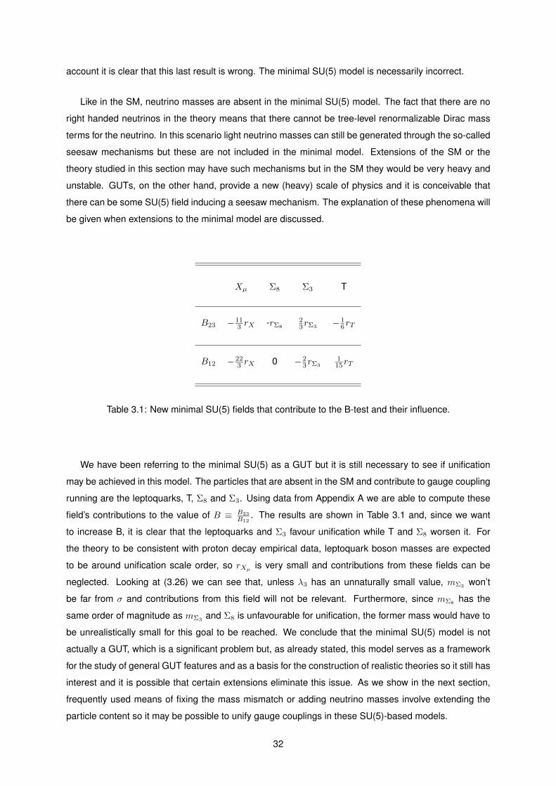
account it is clear that this last result is wrong. The minimal SU(5) model is necessarily incorrect.

Like in the SM, neutrino masses are absent in the minimal SU(5) model. The fact that there are no

right handed neutrinos in the theory means that there cannot be tree-level renormalizable Dirac mass

terms for the neutrino. In this scenario light neutrino masses can still be generated through the so-called

seesaw mechanisms but these are not included in the minimal model. Extensions of the SM or the

theory studied in this section may have such mechanisms but in the SM they would be very heavy and

unstable. GUTs, on the other hand, provide a new (heavy) scale of physics and it is conceivable that

there can be some SU(5) field inducing a seesaw mechanism. The explanation of these phenomena will

be given when extensions to the minimal model are discussed.

Xµ Σ8 Σ3 T

B23 − 113 rX -rΣ8

23rΣ3 − 1

6rT

B12 − 223 rX 0 − 2

3rΣ3

115rT

Table 3.1: New minimal SU(5) fields that contribute to the B-test and their influence.

We have been referring to the minimal SU(5) as a GUT but it is still necessary to see if unification

may be achieved in this model. The particles that are absent in the SM and contribute to gauge coupling

running are the leptoquarks, T, Σ8 and Σ3. Using data from Appendix A we are able to compute these

field’s contributions to the value of B ≡ B23

B12. The results are shown in Table 3.1 and, since we want

to increase B, it is clear that the leptoquarks and Σ3 favour unification while T and Σ8 worsen it. For

the theory to be consistent with proton decay empirical data, leptoquark boson masses are expected

to be around unification scale order, so rXµ is very small and contributions from these fields can be

neglected. Looking at (3.26) we can see that, unless λ3 has an unnaturally small value, mΣ3won’t

be far from σ and contributions from this field will not be relevant. Furthermore, since mΣ8 has the

same order of magnitude as mΣ3and Σ8 is unfavourable for unification, the former mass would have to

be unrealistically small for this goal to be reached. We conclude that the minimal SU(5) model is not

actually a GUT, which is a significant problem but, as already stated, this model serves as a framework

for the study of general GUT features and as a basis for the construction of realistic theories so it still has

interest and it is possible that certain extensions eliminate this issue. As we show in the next section,

frequently used means of fixing the mass mismatch or adding neutrino masses involve extending the

particle content so it may be possible to unify gauge couplings in these SU(5)-based models.

32

3.3 SU(5) Extensions

As we saw in the previous section, the minimal SU(5) has several problems that make it incompatible

with experimental data. Despite this, the fact that this model quantizes electric charge and predicts the

correct charges for all fermions, combined with the fact that unification almost happens, giving estimates

for the unification scale that are consistent with the bounds imposed by proton decay, justify further

pursuit of SU(5) GUTs. The rest of this chapter will be a summary of some frequently seen extensions

of the minimal model. These extended models will be divided in two classes, according to the way

in which the problem of the wrong relationship between the masses of the down quarks and charged

leptons is solved: there are non-renormalizable models, where the particle content doesn’t need to be

enlarged and renormalizable models, where the particle content has to be enlarged.

3.3.1 Non-Renormalizable Models

In this case the Yukawa sector is changed by addition of non-renormalizable terms. A theory like this

is, by definition, incomplete. The reason why it is still worthwhile to work is such a set up is that, since

there are other problems anyway, one can consider the existence of a larger theory that will ultimately

solve all the problems and give consistent effective low energy Yukawas. The non-renormalizable terms

added are [45]

∆LY =5FY(1)5 10F

(Φ

Λ5H

)∗+ 5FY

(2)5

(Φ

Λ10F

)5∗H +

1

8ε510FY

(1)10 10F

(Φ

Λ5H

)+

+1

8ε510FY

(2)10

(Φ

Λ10F

)5H +H.c.,

(3.41)

where Φ is a scalar singlet and Λ is the cut-off scale where the effective operators stop being valid. It

can be taken to be the Planck scale. Considering only the terms with the Higgs doublet we get

Yd = Y T5 −√

3

5

v

ΛY

(1)5 +

2√15

v

ΛY

(2)5 (3.42)

Ye = Y5 −√

3

5

v

ΛY

(1)5 −

√3

5

v

ΛY

(2)5 (3.43)

Yu = −1

2(Y10 + Y T10) +

3

2√

15

v

Λ(Y

(1)10 + Y

(1)T10 )− 1

4√

15

v

Λ(2Y

(2)10 − Y10(2)T ). (3.44)

These new Yukawa matrices have enough adjustable parameters to fit the experimental data.

There is still no gauge unification because the new Yukawas do not alter the running of the theory’s

gauge couplings. This unification can be achieved if new fields are added. At the same time, one

can add certain fields to generate light neutrino masses through seesaw mechanisms. Therefore, both

the unification and the neutrino mass problems can be simultaneously solved by introducing the fields

necessary for the occurrence of seesaw mechanisms that will be described in the end of this chapter.

33

3.3.2 Renormalizable Models

It is possible to ”fix” the relationship between down quark and charged lepton masses of the minimal

model without sacrificing renormalizability. This is done by adding a new scalar representation that can

couple with the fermion fields without changing the breaking pattern. In order to achieve this, we choose

a representation that acquires a non-vanishing vev alongside the SM Higgs by participating in the Higgs

Mechanism. For this to happen the new representation should contain an SU(2) doublet and have an

SU(3)C × U(1)Q invariant vev structure.

A convenient and usual choice is the 45H [46], which verifies the previously stated conditions. It is

derived from 10⊗ 5 = 5⊕ 45 and can be decomposed as

45 = (8, 2, 1/2)⊕ (6, 1,−1/3)⊕ (3, 2,−7/6)⊕ (3, 1, 4/3)⊕ (3, 3,−1/3)⊕ (3, 1,−1/3)⊕ (1, 2, 1/2)), (3.45)

in terms of GSM quantum numbers. The penultimate representation can be identified as a new scalar

colour triplet, T2, and the last one can be identified as a new SU(2)doublet scalar, H2. We can write this

decomposition in a more convenient notation as

45H = S(8,2) ⊕ S(6∗,2) ⊕ S(3∗,2) ⊕ S(3∗,1) ⊕∆⊕ T2 ⊕H2. (3.46)

The vev of the 5H and 45H fields need to be in a correct configuration if we want to reproduce the

SM spontaneous symmetry breaking. For the 5H this is given by

〈5H〉T = (0, 0, 0, 0, v5). (3.47)

In the 45H case, we note that this representation obeys

45αβγ = −45βαγ (3.48)

because the upper indexes come from the completely anti-symmetric 10 representation, which also

implies

(45H)ααγ = 0. (3.49)

Considering this, the vev structure is [47,48]

〈45α5Hβ〉 = v45(δβα − 4δα4 δ

4β), α, β = 1, ..., 4. (3.50)

Finally, these vev combine to give the SM’s v through [49]

v2 ≡ |v5|2 + 24|v45|2 = (√

2GF )−1, (3.51)

where GF is the Fermi constant.

With the addition of the new scalar representation the most general Yukawa sector of the Lagrangian

34

is, in simplified form

− LY =ε54

((Γ1u)ij10i10j5H + (Γ2

u)ij10i10j45H) +√

2((Γ1d)ij10i5

∗j5H + (Γ2

d)ij10i5∗j45∗H), (3.52)

where i,j are generation indices and the Γs are Yukawa matrices. It should be noted that Γ1u is symmetric

and Γ2u is anti-symmetric. Substituting (3.47) and (3.50) in (3.52) we find that, when 5H and 45H acquire

vevs, we get new mass matrices for the fermions:

Mu = v′Γ1u + 2v45Γ2

u, (3.53)

Md = v′∗Γ1d + 2v∗45Γ2

d, (3.54)

MTe = v′∗Γ1

d − 6v∗45Γ2d. (3.55)

A consequence of this is that

Md −MTe = 8v∗45Γ2

d, (3.56)

so the charged lepton and down quark mass matrices are no longer predicted to be equal above unifi-

cation scale. Notice that the presence of Γ1d in Md and Me is very important for these two last matrices

to be different in a way that can solve the mass mismatch problem, otherwise they would just be differ

by a multiplicative factor and the problem would remain.

S(8,2) S(6∗,1) S(3∗,2) S(3∗,1) ∆ T2 H2

B23 − 23rS(8,2)

− 56rS(6∗,1)

16rS(3∗,2)

− 16rS(3∗,1)

23r∆ − 1

6rT2

16rH2

B12 − 815rS(8,2)

215rS(6∗,1)

1715rS(3∗,2)

1615rS(3∗,1)

− 95r∆

115rT2

− 115rH2

Table 3.2: Contributions to the B-test from 45H fields.

The new fields associated with 45H alter the running of SM gauge couplings, with their contributions

to the B test displayed in Table 3.2. Most of these fields have an unfavourable impact on unification

attempts, with the exceptions being ∆ and H2. This last field has a very positive effect as its mass is

expected to be low (of the electroweak scale order). As for ∆, this field contributes to proton decay so

its mass is constrained to be around 1010 GeV or higher. However, if the fields from 45H that make B

smaller have high masses that turn their contributions negligible, this value for the ∆ mass is consistent

with unification.

Extending the minimal SU(5) model by adding a 45H scalar representation leads to a theory where

gauge coupling unification may occur and the mass mismatch problem is no longer present. This comes

at the cost of increasing the theory’s number of parameters, while new naturality problems arise as

35

proton decay and unification constraints force fields from the same 45H representation to have very

different masses but, overall, this extension improves the model, making it more realistic and a proper

GUT. Although there are still no neutrino masses this issue can be solved, as we will see, by introducing

seesaw mechanisms.

3.3.3 Seesaw Mechanisms

As pointed out in the beginning of this chapter, a very relevant deficiency of the SM is the absence of

neutrino masses, but this problem is yet to be addressed in the context of GUTs. Although we could

consider simply adding right-handed neutrinos to the theory so these particles would acquire mass in the

same way as all other fermions, the relative smallness of neutrino masses suggests a different approach:

seesaw mechanisms. In the rest of this chapter we will make a brief review of the most usual types of

seesaw (types I, II and III) and this will be done having the SM as background because it is simpler to

understand these processes in this framework and because our main interest regarding neutrinos is in

their low-energy phenomenology (that is, at energy scales bellow the GUT one, where the gauge group

is GSM ). Furthermore, as we will see in the next chapter, once these mechanisms are understood they

can easily be applied in the context of GUTs.

Figure 3.2: Diagram associated with th d=5 Weinberg operator.

Seesaw mechanisms are characterized by the introduction of new heavy particles in the theory,

with masses that may reach the GUT scale. Tree-level exchange of these particles (depicted in Fig.

3.2) generates a d=5 Weinberg operator, which is the lowest order operator that can lead to Majorana

neutrino masses [50, 51]. The Lagrangian term associated with this is, after integrating-out the heavy

fields,

LWeinberg = −zαβ

Λ(lLαH)C(lLβH)T +H.c., (3.57)

where Λ is the high-energy physics cutoff scale and zαβ are complex constants. Upon SSB this last

equation becomes

LWeinberg = −1

2mαβν ¯νLαν

cLβ +H.c.+ ..., (3.58)

where mαβν = v2zαβ/Λ is the 3 × 3 effective neutrino matrix. It can be seen in what comes next that

36

larger masses of the new fields lead to smaller mνs, hence the designation of seesaw. It should be

pointed out that the calculations performed until the end of this chapter are not exact as only first-order

perturbation theory is used and some channels are ignored in the diagrams that are studied but our

simplified procedure is enough, in this high mass limit, to clarify the flavour structure of the neutrino

mass matrix and its dependence on the new field’s masses.

Type 1 Seesaw

In this type of seesaw the new heavy particles are nR right-handed neutrino fields νRi, with quantum

numbers given by (1,1,0) [52, 53]. Taking this into account, the Lagrangian of the original theory is

modified to

LI = LSM +i

2νRi�∂νRi − Y αiν lLαHνRi −

1

2M ijR

¯νcRiνRj +H.c., (3.59)

where Yν is a 3 × nR complex and arbitrary Yukawa matrix while MR is a nR × nR symmetric matrix.

Before seeing how the exchange of these νRi leads to small neutrino masses it is convenient to change

basis in order to have the new fields as mass eigenstates:

νRi = RijRNRj , RTRMRRR = dR = diag(M1, ...,MnR). (3.60)

Figure 3.3: Feynman diagram representing the exchange of heavy particles that generates type I see-saw.

The Lagrangian in (3.59) may now be written as

LI = LSM + iNRi�∂NRi − Y αiR lLαHNRi −1

2dijRN

cRiNRj +H.c., (3.61)

where YR = YνRR. Comparing the Feynman diagram for νRi exchange (Fig. 3.3) with Fig. 3.2 and

comparing (3.61) with (3.57) we obtain

zαβ

∆∝ Y αiR

1

�p−MiY βiR . (3.62)

It has already been stated that the Mi are much larger than the electroweak scale so we can make the

following approximation:zαβ

∆' −Y αiR

1

MiY βiR = −Y αiR

1

diiRY βiR . (3.63)

37

Recalling (3.60) we can write

zαβ

∆'− Y αiR (diiR)−1Y βiR = −(YRd

−1R Y TR )αβ = −(YνRR(RR)−1(MR)−1(RTR)−1RTRY

Tν )αβ =

= −(YνM−1R Y Tν )αβ .

(3.64)

To get the desired result, the effective mass matrix of light neutrinos, we use (3.57):

mν = −v2YνM−1R Y Tν = −mDM

−1R mT

D, (3.65)

with mD = vYν . We can easily see that large values of MR lead to small mν , as we wanted in order to

reproduce experimental data.

Type 2 Seesaw

In type II seesaw we introduce (ar least) one SU(2) scalar triplet ∆ = {∆1, ∆2, ∆3} with quantum num-

bers given by (1,3,1) [54–58]. As these fields are not singlets, some care must be taken to ensure that

terms involving them are gauge invariant. We can use the Pauli matrices to write them as

∆ = ∆iσi

2=

1

2

∆3 ∆1 − i∆2

∆1 + i∆2 −∆3

. (3.66)

Choosing the basis where T 3 is a 3× 3 diagonal matrix, the following relations hold:

∆ =

∆+√

2−∆++

∆0 −∆+√

2

⇒ Q(∆) =

∆+√

2−2∆++

0 −∆+√

2

. (3.67)

As the new scalar fields transform under SU(2) according to

´∆ = e−iT

aωa∆, (T a)ij = −iεaij , (3.68)

we see that ∆ transforms according to ´∆ = U∆U†, where U is an unitary matrix. The possible terms

involving ∆, namely lL∆†lcL and HT ∆∆ are still not gauge invariant as

¯lL∆†C

¯lTL = lLU

†U∆†U†U∗ClLT

= lL∆†U†U∗ClLT, ´HT ´∆ ´H = HTUTU∆U†UH = HTUTU∆H.

(3.69)

Finally, to achieve invariance, we rotate the fields using the Pauli matrix σ2, as we did for the Higgs field

in the previous chapter:

∆ = iσ2∆ =

∆0 −∆+√

2

−∆+√

2∆++

. (3.70)

The fields ∆ transform as ∆ = U∗∆U† and the possible terms associated with the new scalars are

38

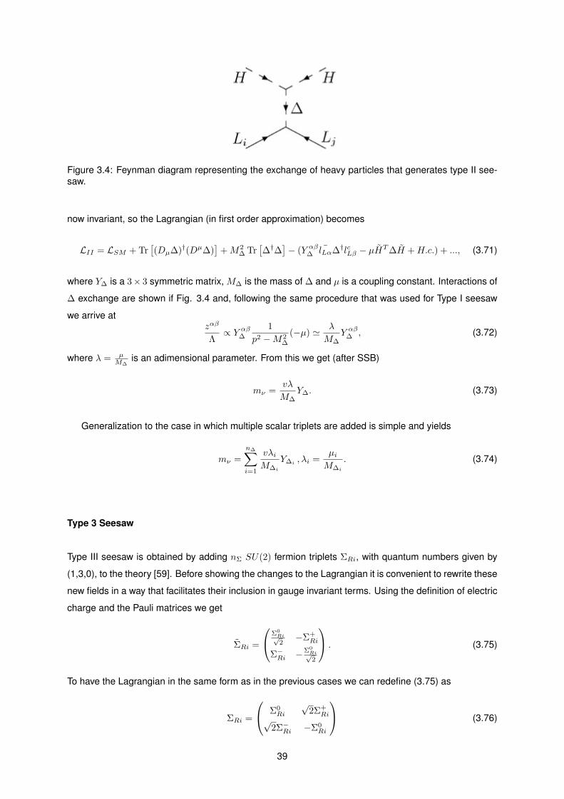
Figure 3.4: Feynman diagram representing the exchange of heavy particles that generates type II see-saw.

now invariant, so the Lagrangian (in first order approximation) becomes

LII = LSM + Tr[(Dµ∆)†(Dµ∆)

]+M2

∆ Tr[∆†∆

]− (Y αβ∆

¯lLα∆†lcLβ − µHT∆H +H.c.) + ..., (3.71)

where Y∆ is a 3× 3 symmetric matrix, M∆ is the mass of ∆ and µ is a coupling constant. Interactions of

∆ exchange are shown if Fig. 3.4 and, following the same procedure that was used for Type I seesaw

we arrive atzαβ

Λ∝ Y αβ∆

1

p2 −M2∆

(−µ) ' λ

M∆Y αβ∆ , (3.72)

where λ = µM∆

is an adimensional parameter. From this we get (after SSB)

mν =vλ

M∆Y∆. (3.73)

Generalization to the case in which multiple scalar triplets are added is simple and yields

mν =

n∆∑i=1

vλiM∆i

Y∆i, λi =

µiM∆i

. (3.74)

Type 3 Seesaw

Type III seesaw is obtained by adding nΣ SU(2) fermion triplets ΣRi, with quantum numbers given by

(1,3,0), to the theory [59]. Before showing the changes to the Lagrangian it is convenient to rewrite these

new fields in a way that facilitates their inclusion in gauge invariant terms. Using the definition of electric

charge and the Pauli matrices we get

ΣRi =

Σ0Ri√2−Σ+

Ri

Σ−Ri −Σ0Ri√2

. (3.75)

To have the Lagrangian in the same form as in the previous cases we can redefine (3.75) as

ΣRi =

Σ0Ri

√2Σ+

Ri√2Σ−Ri −Σ0

Ri

(3.76)

39

and, finally,

LIII = LSM +i

2tr(ΣRiDΣRi)− Y αiT lLαΣRiH −

1

2M ij

Σ tr(ΣRiΣRj) +H.c., (3.77)

where YT is a 3 × nΣ arbitrary complex Yukawa matrix and MΣ is a nΣ × nΣ symmetric matrix. In this

case the Weinberg operator is generated by the exchange process shown in Fig. 3.5 and, due to the

similarities between this situation and Type I seesaw we can obtain the light neutrinos effective mass

matrix simply by comparing (3.77) with (3.61):

zαβ

Λ' −(YTM

−1Σ Y TT )αβ ⇒ −v2YTM

−1Σ Y TT = −mTM

−1Σ mT

T , (3.78)

where mT = vYT .

Figure 3.5: Feynman diagram representing the exchange of heavy particles that generates type IIIseesaw.

40

Chapter 4

Discrete Symmetries and Proton

Decay

In this chapter we introduce the Adjoint SU(5) model with intention of building a realistic and predictive

theory from it. We investigate proton decay and the possibility of using discrete symmetries to simulta-

neously alleviate constraints related to this process and reduce the number of Yukawa parameters.

4.1 Adjoint-SU(5) Model

The Adjoint SU(5) model can be considered a natural consequence of our discussion so far because it

is obtained from the minimal SU(5) model by adding a 45H scalar representation to solve the mass mis-

match problem and nρ adjoint fermionic fields ρ(24) to generate light neutrino masses through seesaw

mechanisms [17]. This choice of the adjoint representation follows from the fact that, decomposing it in

terms of GSM quantum numbers,

ρ(24) = ρ8 ⊕ ρ3 ⊕ ρ(3,2) ⊕ ρ(3∗,2) ⊕ ρ0, (4.1)

one sees that it contains a singlet and an SU(2) triplet so both Type I and Type III seesaw are induced.

The main effects of adding a 45H scalar to the minimal SU(5) were already covered in section 3.3.2,

therefore, we will now focus on changes brought on by the ρ(24) fields. We assume that these fields

acquire unconstrained Majorana masses, so the most general Yukawa sector consistent with renormal-

izability is now given by

−LY =ε54

((Γ1u)ij10i10j5H + (Γ2

u)ij10i10j45H) +√

2((Γ1d)ij10i5

∗j5H + (Γ2

d)ij10i5∗j45∗H)+

+MklTr(ρkρl) + λklTr(ρkρlΣ) + (Γ1ν)ik5∗i ρk5H + (Γ2

ν)ik5∗i ρk45H +H.c.,

(4.2)

where k, l = 1, ..., nρ, M is a symmetric nρ × nρ Majorana mass matrix and λ, Γ1ν and Γ2

ν are Yukawa

matrices (λ is symmetric).

41

When the adjoint scalar 24H gets a vev we have ρ(24) masses given by

M0 =1

4(M − σ√

30λ),

M3 =1

4(M − 3σ√

30λ),

M8 =1

4(M +

2σ√30λ),

M(3,2) = M(3∗,2) =1

4(M − σ

2√

30λ).

(4.3)

From now on, since we are interested in analysing Types I and III seesaw, we will no longer consider the

ρ8, ρ(3,2) and ρ(3∗,2) fields. Looking at (3.52) and the analogous equations, (3.56) and (3.72) we notice

that the light neutrino masses are proportional to v2, where v is the SM Higgs doublet’s vev. On the

other hand, we saw in section 3.3.2. that, in a framework with a 45H scalar representation, this constant

v appears as a combination of the H1 and H2 vevs. It is, then, convenient to make a basis change in

order to have one Higgs double H with a vev of v and another one, H, without vev:HH

=

cosβ sinβ

− sinβ cosβ

H1

H2

, (4.4)

with tanβ ≡ v45/v5. In this new basis we get, from (4.2) and the decompositions of ρ(24) fields shown

in Appendix B, the following Yukawa interactions involving these fields and SM fermions:

−LY =

√15

2

[cosβ

5(Γ1ν)ik + sinβ(Γ2

ν)ik

]lTi iσ2ρ0kH+

+

√15

2

[− sinβ

5(Γ1ν)ik + cosβ(Γ2

ν)ik

]lTi iσ2ρ0kH+

+1√2

[− cosβ(Γ1

ν)ik + 3 sinβ(Γ2ν)ik

]lTi iσ2ρ3kH+

+1√2

[sinβ(Γ1

ν)ik + 3 cosβ(Γ2ν)ik

]lTi iσ2ρ3kH +H.c..

(4.5)

Comparing this result with the descriptions of Type I and Type II seesaw in the last chapter, we obtain

(mν)ij = −(mD0 M

−10 mD

0

T)ij − (mD

3 M−13 mD

3

T)ij , (4.6)

with

mD0 =

√15v

2(cosβ

5Γ1ν + sinβΓ2

ν), mD3 =

v√2

(− cosβΓ1ν + 3 sinβΓ2

ν). (4.7)

Since M0 and M3 are unconstrained Majorana masses they can have very high values, making the left-

handed neutrino masses very small, in accordance with experimental evidence. There is another type

of seesaw that can be induced by the ρ8, radiative seesaw [60–63], but it was ignored for simplicity sake.

We can do this because the new contributions are very suppressed if one assumes mρ3k � mρ0k and

mρ8k � mρ3k [64,65].

A discussion of unification and associated constraints is postponed until the next chapter, where we

42

choose a particular value of nρ and a discrete symmetry is incorporated in the theory.

4.2 Proton Decay in the Adjoint SU(5) model

It has been mentioned, in the previous chapter, that proton decay is a common problem in GUTs. This

process is absent in the SM due to an accidental symmetry that preserves B − L and the fact that the

proton is the lightest baryon. In GUTs this symmetry is lost as there are new particles that can mediate

proton decay, which constitutes a problem for such theories because no event of this kind has been

observed so far. This last aspect means that protons have a very large lifetime and, consequently, any

amplitude that contributes to the process must be very small if a model is to describe elementary particle

interactions correctly.

The sources of proton decay in the Adjoint model are the leptoquarks and coloured scalar triplets.

When theX and Y bosons were introduced it was pointed out that they can connect quark lines to lepton

lines, since they are SU(3) triplets and SU(2) doublets. Because of this there will be new interactions

that are forbidden in the SM and it is important to study them in order to discover their possible conse-

quences. The interactions between bosons and fermions come from the terms with covariant derivatives

of the fermion fields, which are given by

LF = i1

2Tr{Ψ10��DΨ10}+ iΨ5��DΨ5, (4.8)

so one gets

LFint = −g5Tr{Ψ10γµAµΨ10}+ g5Ψ5γ

µATµΨ5. (4.9)

We are only interested in the new interactions so the terms of relevance in this context are the ones

involving the new bosons:

LXY = −g5Tr{Ψ10γµAXµ Ψ10}+ g5Ψ5γµ(AXµ )TΨ5. (4.10)

Since the X and Y bosons belong to the same SU(5) representations and have the same quantum

numbers, as well as the same mass, they can be regarded as the same field with two indexes, that is,

(Xµ)aα where a is an SU(3)C index, α is an SU(2)L index and a = 1→ X, a = 2→ Y . With this in mind,

(4.10) may be written as

LXY =g5√

2

[((dc)

αγµεabLb − ecεbaγµqαb + qβaγ

µεαβγucγ)(Xµ)aα]

+H.c. . (4.11)

By inspection of the above expression it can be seen that quarks may become leptons (and vice-versa)

in interactions mediated by these bosons. One important consequence of this is that protons can decay.

In order to get an idea of the constraints that the model parameters in (4.11) must obey for there

to be accordance with experimental data it is useful to make an estimation of the proton decay width

associated these terms. Since this is a low energy process, the analysis can be done using effective

43

operators. The equations of motion for a given field φ are

∂µ∂L

∂(∂µφ)− ∂L∂φ

= 0 (4.12)

and when a φ is much heavier than the energy scale of the event being studied, as in the leptoquark

case, the field can be integrated out (its derivatives are very small) so (4.12) is approximately

∂L∂φ

= 0. (4.13)

Before applying equation (4.13) to the leptoquark fields it is still necessary to add the new bosons

mass term,

LMV= −M

2V

2(Xc

µ)αa (Xµ)aα, (4.14)

to (4.11) so that LXY +LMVhas all relevant information of these fields as well as their interactions with

fermions. One can, now, use the equations of motion to get

(Xcµ)αa =

√2g5

M2X

{(dc)αγµεabL

b − ecεbaγµqαb + qβaγµεαβγucγ

}, (4.15)

while the conjugate field is given by the Hermitian conjugate of the previous expression. Substituting in

(4.11) yields

LXeff =g2

5

M2X

εαβγ(uc)αγµqaβ{ecεabγ

µqγb + (dc)γγµεabLb}

+H.c., (4.16)

which are the dimension 6 effective operators.

To get an estimation of the proton decay width associated with (4.16) one can consider the following

decay channel:

p→ π0e+, (4.17)

that is, one up quark becomes a positron and the down quark becomes an anti-up quark. The amplitudes

contributing to this process are

M1 =g2

5

M2V

εαβγ(uc)αuβ ecγµγµdγ , M2 =

g25

M2V

εαβγ(uc)αγµuβ(dc)γγµe, (4.18)

so one can state that [66]

Γpd ∼ α25

m5p

M4X

. (4.19)

Using the most restrictive constraints on the proton lifetime available at this time [67], which are

τ(p→ π0e+) > 1.4× 1034years, (4.20)

and the fact that unification requires 26 ≤ α−15 ≤ 35 [68], we obtain

MV > (4.9− 5.7)× 1015GeV. (4.21)

44

It is being assumed that MV and the unification scale are of the same order of magnitude so (4.21)

constrains the region where gauge couplings can unify. There is enough freedom in the Adjoint model

for these constraints to be respected, therefore, leptoquark mediated proton decay is not a big problem

in this context.

It was pointed out, in the last chapter, that the 5H scalar multiplet includes not only a Higgs-like SU(2)

doublet but also a coloured scalar triplet. Since this triplet is absent in the SM it is important to study

its consequences in the Adjoint model and SU(5) GUTs in general. Its interactions with fermions come

from the Yukawa Lagrangian in (4.2):

− L5H−fermionY =

εαβγδη4

(Γ1u)ij10αβi 10γδj (5H)η +

√2(Γ1

d)ij10αβi 5∗jα(5∗H)β , (4.22)

where the i,j are generation indexes and α, β, γ, δ, η are SU(5) indexes. Some other terms in (4.2) also

involve the 5H and fermions but not quarks so they are not relevant for the present discussion. Taking

into account the fact that 5H may be written as

5H =

T1

H

, (4.23)

where T1 is the coloured scalar triplet and H is the Higgs-like doublet, (4.22) may be simplified and,

keeping only the terms with T1 we get

(Γ1u)ij(

1

2QiQj + uiCejC)T1 + (Γ1

d)(QiLj + uiCdjC)T ∗1 . (4.24)

After adding the triplet’s mass term,

−m2T1T ∗1 T1, (4.25)

to (4.24), we can repeat the procedure used to obtain the effective operators for leptoquark mediated

proton decay to get(Γ1u)ij(Γ

1d)kl

M2T1

[1

2(QiQj)(QkLl) + (ucie

cj)(u

ckdcl )

], (4.26)

the dimension 6 effective operators contributing to the decays by means of T1 bosons exchange.

There is another coloured scalar triplet in the Adjoint model, T2, which belongs to the 45H scalar

representation. Starting form the Yukawa Lagrangian and retaking the steps already described for the

leptoquarks and T1 one arrives at the following effective operators:

4(Γ2u)ij(Γ

2d)kl

M2T2

(uciecj)(u

ckdcl ). (4.27)

The 45H multiplet contains other coloured representations that may lead to proton decay, specifically,

the (3∗, 1, 4/5) triplet and the three triplets ∆−1/3, ∆2/3 and ∆−4/3 (the superscript refers to the electric

charge), which belong to the (3, 3,−1/5) triplet-triplet. By expanding the Lagrangian terms involving

these fields one can see that (3∗, 1, 4/5) and ∆−4/3 make no contribution for proton decay as they only

couple to pairs of up-quarks while (Γ2u) is antisymmetric (therefore it cannot couple two equal particles).

45

For the ∆−1/3 and ∆2/3 fields the effective operators are

(Γ2u)ij(Γ

2d)kl

2M2∆−1/3

[(uidj)(ukel) + (uidj)(dkνl)] (4.28)

and

− (Γ2u)ij(Γ

2d)kl

2M2∆2/3

(didj)(ukνl) (4.29)

respectively.

All sources of proton decay in the Adjoint model are now accounted for. One could approach the

scalar mediated case in the same way as the leptoquark mediated case, by estimating the decay widths

associated with it and, consequently, the constraints imposed on the masses of these scalars, but an-

other strategy will be used. The main reason for this is that, unlike the leptoquark masses, the scalar

masses cannot be raised above a certain threshold without creating or worsening doublet-triplet splitting

problems. Therefore, we will try to suppress scalar mediated proton decay in a different way. Since

these processes depend on the Yukawa matrices of the model, this suppression may be achieved by

imposing constraints on these matrices. However, even if we forbid these processes at tree-level and

take into account the fact that scalar-mediated decays are proportional to the Yukawa terms which are,

in general, smaller than gauge couplings, we cannot eliminate the splitting problems. This endeavour is

still worthwhile because it loosens the constraints on scalar triplet masses.

4.3 Conditions for Proton Decay Suppression and Discrete Sym-

metries

By inspection of the effective operators for scalar mediated proton decay it becomes apparent that this

possess can be eliminated (at tree level) if certain elements of the Yukawa matrices are zero. These

matrices are arbitrary and complex, so it is convenient to find a way of ”forcing” specific elements to

be annulled. This can be done by changing the gauge group to SU(5) × A where A is a discrete

abelian group and assigning A charges to the fields in such a way that some terms are not invariant

for transformations from this group and, therefore, cannot be present. It is important to note that this

discrete symmetry survives below unification scale only if the field responsible for the SU(5) SSB has

no A group charge.

The first step that must be taken in order to achieve this is to identify the conditions that the Yukawa

matrices must verify for proton decay to be forbidden at tree level. Starting form the effective operators

obtained in the previous section one can draw the diagrams that contribute to this process and infer

which Yukawa parameters have to be zero. For T1 mediated proton decay these operators are given in

(4.26) and the corresponding diagrams are shown in Figure 4.1.

The conditions that are to be imposed on Γ1u and Γ1

d are summarized in Table 4.1.

It is important to note that decays with third generation fermions (other than neutrinos) or charmed

quarks in the final state are already forbidden as these particles are heavier than protons and to re-

46

Figure 4.1: Diagrams associated with T1 mediated proton decay. Some diagrams represent severalprocesses as Q and L can correspond to different particles.

Diagram A B C D

Γ1u-exclusive conditions (Γ1

u)11 = 0(Γ1u)11 = 0,

(Γ1u)12 = 0

(Γ1u)11 = 0,

(Γ1u)12 = 0

(Γ1u)11 = 0,

(Γ1u)12 = 0

Γ1d-exclusive conditions

(Γ1d)11 = 0,

(Γ1d)12 = 0,

(Γ1d)21 = 0,

(Γ1d)13 = 0,

(Γ1d)23 = 0,

(Γ1d)22 = 0

(Γ1d)11 = 0,

(Γ1d)12 = 0,

(Γ1d)13 = 0

(Γ1d)11 = 0

(Γ1d)11 = 0,

(Γ1d)12 = 0

Table 4.1: Sufficient conditions for proton decay suppression in the T1 mediated case.

member that, by definition, Γ1u is symmetric and Γ2

u is antisymmetric. Since the diagrams in Fig. 4.1 are

the only ones involving Γ1u and Γ1

d we can already list the distinct, independent, sets of conditions these

matrices must obey in order for our goal to be achieved:

→ (Γ1u)11 = 0, (Γ1

d)11 = 0, (Γ1d)12 = 0, (Γ1

d)13 = 0, (4.30)

→ (Γ1u)11 = 0, (Γ1

u)12 = 0, (4.31)

→ (Γ1d)11 = 0, (Γ1

d)12 = 0, (Γ1d)21 = 0, (Γ1

d)22 = 0, (Γ1d)13 = 0, (Γ1

d)23 = 0. (4.32)

For T2 mediated proton decay we use (4.27) to obtain the diagrams shown in Figure 4.2.:

The conditions required for these processes to vanish are presented in table 4.2.:

Repeating these steps for ∆−1/3 mediated proton decay and using (4.28) the relevant diagrams are

47

Figure 4.2: Diagrams associated with T2 mediated proton decay.

Diagram E F

Γ2u-exclusive conditions (Γ2

u)11 = 0,(Γ2u)12 = 0

(Γ2u)11 = 0,

(Γ2u)12 = 0

Γ2d-exclusive conditions (Γ2

d)11 = 0(Γ2d)11 = 0,

(Γ2d)12 = 0

Table 4.2: Sufficient conditions for proton decay suppression in the T2 mediated case.

Figure 4.3: Diagrams associated with ∆−1/3 mediated proton decay.

and the sufficient conditions for them to vanish are

Finally, regarding ∆2/3 induced proton decay, we can use (4.29) to obtain the remaining proton decay

diagram:

48

Diagram G H I J

Γ2u-exclusive conditions (Γ2

u)11 = 0(Γ2u)11 = 0,

(Γ2u)12 = 0

(Γ2u)11 = 0

(Γ2u)11 = 0,

(Γ2u)12 = 0

Γ2d-exclusive conditions (Γ2

d)11 = 0,(Γ2d)12 = 0

(Γ2d)11 = 0,

(Γ2d)12 = 0

(Γ2d)11 = 0,

(Γ2d)12 = 0,

(Γ2d)21 = 0,

(Γ2d)22 = 0,

(Γ2d)23 = 0

(Γ2d)11 = 0,

(Γ2d)12 = 0,

(Γ2d)13 = 0

Table 4.3: Sufficient conditions for proton decay suppression in the ∆−1/3 mediated case.

Figure 4.4: Diagrams associated with ∆2/3 mediated proton decay.

This process is forbidden if

Diagram K

Γ2u-exclusive conditions (Γ2

u)11 = 0,(Γ2u)12

Γ2d-exclusive conditions

(Γ2d)11 = 0,

(Γ2d)12 = 0,

(Γ2d)13 = 0

Table 4.4: Sufficient conditions for proton decay suppression in the ∆2/3 mediated case.

Combining the results from tables 4.2, 4.3 and 4.4 we can compile the conditions Γ2u and Γ2

d must

verify to suppress proton decay:

→ (Γ2u)11 = 0, (Γ2

d)11 = 0, (Γ2d)12 = 0, (Γ2

d)13 = 0 (4.33)

→ (Γ2u)11 = 0, (Γ2

u)12 = 0 (4.34)

→ (Γ2d)11 = 0, (Γ2

d)12 = 0, (Γ2d)21 = 0, (Γ2

d)22 = 0, (Γ2d)13 = 0, (Γ2

d)23 = 0. (4.35)

If one of (4.30), (4.31) or (4.32) and one of (4.33), (4.34) or (4.35) is true then there is no scalar mediated

proton decay at tree level in the Adjoint model. We now have the right setup to start looking for discrete

abelian symmetries that can lead to these conditions being satisfied.

This was achieved by writing a computer program in the C language that, for a given symmetry, tests

all possible charge assignments that the fields involved in proton decay may have to check weather the

constraints discussed in the previous paragraph are obeyed. The symmetries that were considered are

49

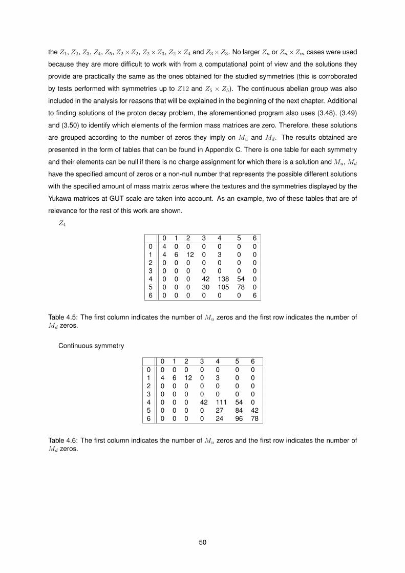
the Z1, Z2, Z3, Z4, Z5, Z2×Z2, Z2×Z3, Z2×Z4 and Z3×Z3. No larger Zn or Zn×Zm cases were used

because they are more difficult to work with from a computational point of view and the solutions they

provide are practically the same as the ones obtained for the studied symmetries (this is corroborated

by tests performed with symmetries up to Z12 and Z5 × Z5). The continuous abelian group was also

included in the analysis for reasons that will be explained in the beginning of the next chapter. Additional

to finding solutions of the proton decay problem, the aforementioned program also uses (3.48), (3.49)

and (3.50) to identify which elements of the fermion mass matrices are zero. Therefore, these solutions

are grouped according to the number of zeros they imply on Mu and Md. The results obtained are

presented in the form of tables that can be found in Appendix C. There is one table for each symmetry

and their elements can be null if there is no charge assignment for which there is a solution and Mu, Md

have the specified amount of zeros or a non-null number that represents the possible different solutions

with the specified amount of mass matrix zeros where the textures and the symmetries displayed by the

Yukawa matrices at GUT scale are taken into account. As an example, two of these tables that are of

relevance for the rest of this work are shown.

Z4

0 1 2 3 4 5 60 4 0 0 0 0 0 01 4 6 12 0 3 0 02 0 0 0 0 0 0 03 0 0 0 0 0 0 04 0 0 0 42 138 54 05 0 0 0 30 105 78 06 0 0 0 0 0 0 6

Table 4.5: The first column indicates the number of Mu zeros and the first row indicates the number ofMd zeros.

Continuous symmetry

0 1 2 3 4 5 60 0 0 0 0 0 0 01 4 6 12 0 3 0 02 0 0 0 0 0 0 03 0 0 0 0 0 0 04 0 0 0 42 111 54 05 0 0 0 0 27 84 426 0 0 0 0 24 96 78

Table 4.6: The first column indicates the number of Mu zeros and the first row indicates the number ofMd zeros.

50

Chapter 5

Adjoint SU(5) with Discrete Symmetry

Results

In order to obtain a realistic theory from the model described in the previous chapter we review aspects

of low-energy fermion masses and mixings that this theory should be able to reproduce. We also see

that the discrete symmetry used to prevent scalar mediated tree level proton decay may be broken by

quantum gravity effects unless some ”discrete anomaly” cancellation conditions are verified. Finally, we

investigate the possibility of choosing a particular ZN symmetry and assigning charges related to this

group in such a way that these constraints are obeyed, while trying to make the resulting theory as

predictive as possible.

5.1 Criteria for a Realistic Adjoint SU(5)×ZN theory

Estimates of the unification scale put it at much higher energies than the ones accessible to us in

controlled experiments. Because of this, it is impossible to directly check certain relations that are valid

when the GUT gauge group is effective or detect the new heavy fields predicted to exist, but we can make

sure that the theory is consistent with low-energy data, determine unification and proton constraints on

the masses of new fields to find out weather some of them may be detected in the near future and see

if there are new (accurate) relations between low-energy observables not present in the SM.

We start by verifying the theory’s compatibility with low-energy data, for if this fail it loses most of its

interest. In Chapter 2. we introduced the CKM matrix, which contains all the information about quark

mixings at SM scale, so we should verify if there are enough free (quark related) Yukawa parameters

to get this matrix, within 1σ of its experimental values, at such energies. When we talked about quark

mixings it was pointed out that no analogous processes took place in the lepton sector. This was

justified by the absence of neutrino masses in the SM, but, since then, we have managed to generate

light masses for left-handed neutrinos through seesaw mechanisms.

51

5.1.1 Low-Energy Neutrino Phenomenology

Experimental observation of neutrino oscillations strongly suggests that these particles have masses (as

it depends on the square of different neutrino’s masses) and implies a distinction between the interaction

and mass basis, specifically,

ν′α =

3∑j=1

Uαjνj , (5.1)

where U is an unitary matrix, ν′ are interaction eigenstates and the ν are mass eigenstates. After SSB

of the GUT gauge group we may write the lepton masses in the interaction basis as

Lleptonmasses = −Mle′Le′R −

1

2mµν

′Lν′cL +H.c.. (5.2)

The charged lepton mass matrix can be diagonalized by means of a bi-unitary transformation, that is

U†lLMlURl = Dl ≡ diag(me,mµ,mτ ). (5.3)

As for the neutrino Majorana mass matrix, it is symmetric and is multiplied form both sides by the same

vector (in family space), νL, so we diagonalize it using a single unitary matrix,

UTν mνUν = Dν ≡ diag(m1,m2,m3), (5.4)

where the mi represent left-handed neutrino masses. Interaction and mass eigenstates are, then, re-

lated through

l′R = URllR, l′L = ULllL, ν

′L = UννL. (5.5)

Applying these transformations to the charged current in (2.42) we obtain

Lchargedcurrent =gW√

2(u′Lγ

µd′L+ν′Lγµe′L)W+

µ H.c. =gW√

2(uLVCKMγ

µdL+νLU†PMNSeL)W+

µ +H.c., (5.6)

where

UPMNS = U†LlUν =

Ue1 Ue2 Ue3

Uµ1 Uµ2 Uµ3

Uτ1 Uτ2 Uτ3

. (5.7)

For the same number of generations PMNS has more phases than VCKM , as long as the neutrinos

are Majorana particles. This happens because we cannot rephase Uν without altering the neutrino

masses:

Uν → Uνdiag(eiξ1 , eiξ2 , eiξ3)⇒ mj → mje2iξj . (5.8)

We conclude that ξj can only be arbitrary if mj = 0. The PMNS matrix may be written as

UPMNS = diag(eiζe , eiζµ , eiζτ )Uinternaldiag(eiβ1 , eiβ2 , eiβ3), (5.9)

52

where Uinternal has the same number of parameters as VCKM , with ng(ng − 1)/2 Euler angles and

(ng − 1)(ng − 2)/2 Dirac phases. Considering ng = 3, a frequently used way of parametrizing Uinternal

is

Uinternal =

c12c13 s12c13 s13e

−iδ

−s12c23 − c12s23s13eiδ c12c23 − s12s23s13e

iδ s23c13

s12s23 − c12c23s13eiδ −c12s23 − s12c23s13e

iδ c23c13

, (5.10)

with ci ≡ cos θi and si ≡ sin θi for i = 12, 13, 23. We note that all ζα phases are devoid of physical

meaning as they may be eliminated by rephasing the charged lepton fields. This procedure is not

applicable to the Majorana phases βj due to already mentioned reasons. However, only two out of these

three phases (with ng = 3 and no zero neutrino mass) are relevant because we can remove the global

phase (β1 + β2 + β3)/3 and add it to the ζ phases. In fact, the potentially observable quantities involving

βs are 2(β2 − β1) and (β3 − β1).

Then, for any given number of generations, UPMNS has the same number of phases as VCKM plus a

number of Majorana phases equal to the number of Majorana neutrinos minus one, unless one of these

neutrinos has a null mass (experimental data collected so far is consistent with one massless neutrino),

in which case the number of Majorana phases is reduced by one. The UPMNS matrix is very important

in this context as it provides us a way of testing low-energy lepton mixings and neutrino phenomenology

given by a GUT.

5.1.2 Discrete Gauge Symmetry Anomalies

A QFT with a gauge group of SU(5) and a fermion content consisting in ng 5∗, ng 10 and nρ adjoint (24)

representations is anomaly-free. The only possible anomaly in this scenario would be the [SU(5)]3 one

but 5∗ and 10 have opposite contributions while 24 representations do not contribute at all [69]. What

about the SU(5)× ZN case?

At first sight, one would think that no new anomalies arise, as discrete symmetries are not, in general,

constrained by anomaly-freedom conditions. However, it has been argued that quantum gravity effects

violate any non-gauge symmetries. Then, if we want our discrete symmetry to be safe from these effects,

we must make sure they verify certain ”discrete anomaly cancellation” conditions [70]. In order to define

such conditions we note that in continuum theories the ZN discrete symmetries result from breaking an

U(1) gauge symmetry with a scalar field φ of charge Nq that acquires a vev. Therefore, the ”discrete

anomaly” constraints correspond to the requirement that the original U(1) group is anomaly-free.

If we have a discrete ZN gauge symmetry under which the fermion fields transform as Ψi →

exp(i2πqi/N)Ψ1, the U(1) charges before SSB were necessarily of the form

Qi = qi +miN, (5.11)

where qi and mi are integers (qi are the ZN charges). For an SU(5) × U(1) gauge group the possible

53

anomalies are U(1) [SU(5)]2, [U(1)]

3 and U(1)-gravity-gravity, which are proportional to

A1 =∑i

Ti(Qi), (5.12)

where Ti are the quadratic Casimirs,

A2 =∑i

(Qi)3, (5.13)

and

A3 =∑i

Qi, (5.14)

respectively (the sum is over the theory’s fermion representations). We may use (5.11) to redefine the

U(1) charges so these As are annulled, but this is not always possible. In particular, note that, when

using the ZN charges, the As must be proportional to N for this procedure to work (necessary but not

sufficient condition).

We can also consider the existence of heavy fermions that become massive upon SSB and con-

tribute to the anomaly-freedom conditions. There are two types of masses fermions may acquire at this

stage [71]:

-Pairs of different Weyl fermions with charges that verify

QjW1 +QjW2 = pjN, (5.15)

where pj is an integer, combine to get a mass. They contribute an amount of

Tjpj (5.16)

to A1, an amount of

(QjW1)3 + (QjW2)3 = pjN(3Qj2W1 − 3pjNQjW1 + p2

jN2) (5.17)

to A2 and an amount of

pjN (5.18)

to A3.

-One fermion that is an SU(5) singlet gets a Majorana mass and it must verify

Qjχ =1

2p′jN (5.19)

when N is even (there is no contribution to the anomalies when N is odd), pj are integers. A1 is left

unchanged because the Casimir of an SU(5) singlet is zero, A2 is modified by the addition of

1

8p′3j N

3 (5.20)

54

and A3 by the addition of1

2p′jN. (5.21)

Admitting the possibility of having several of these new fields and considering the charge redefinitions

we are free to make, the anomaly-freedom constraints become

∑i

Ti(qi) = rN, (5.22)

∑i

(qi)3 = mN + ηn

N3

8, (5.23)

and ∑i

qi = pN + ηqN

2, (5.24)

where η is 1, 0 for N even, odd, respectively, and the integers r, m, n, p, q are given by

r = −∑i

Timi −∑

heavies

Tjpj , (5.25)

m = −(3∑i

q2imi + 3N

∑i

qim2i +N2

∑i

m3i )

−∑j

pj(3Qj2W1 − 3pjNQ

jW1 + p2

jN2),

n =∑j

p′3j ,

(5.26)

p = −∑i

mi −∑j

pj , q = −∑j

p′j . (5.27)

If the conditions in (5.22), (5.23) and (5.24) are satisfied we still have no guarantee of anomaly-

freedom, since (5.25), (5.26) and (5.27) are diophantine equations that do not always admit solutions.

As we will see later, the new heavy fields introduced in this section may help us achieve a theory without

anomalies, but it can be argued that carefully choosing the characteristics and number of fields to be

added in order to achieve this goal is not natural, so, in this context, the obtained conditions are more

useful in excluding theories that cannot be made anomaly-free (unless some other mechanism comes

into play).

5.1.3 Unification Constraints

An analysis of unification-related constraints on the model’s fields masses can be carried out before

a particular ZN is chosen because the particle content will be the same and tree-level scalar-mediated

proton decay suppression is required in all studied cases (this is not exactly true as relationships between

the masses of the adjoint fermionic fields depend on (4.3), but it has been checked that this does not

significantly affect our discussion, we consider an M with all elements equal to zero except for the ones

in the diagonal for simplicity). From this point onward we consider nρ = 3 as a smaller number could

55

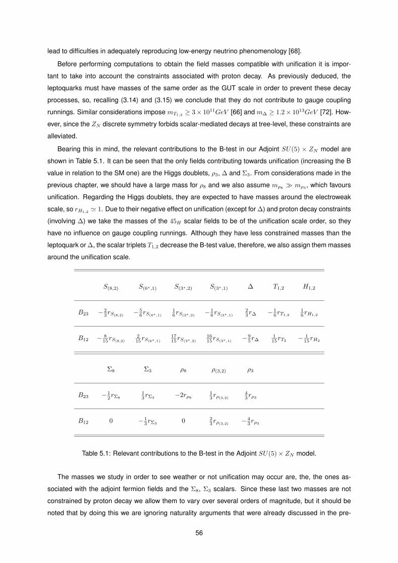
lead to difficulties in adequately reproducing low-energy neutrino phenomenology [68].

Before performing computations to obtain the field masses compatible with unification it is impor-

tant to take into account the constraints associated with proton decay. As previously deduced, the

leptoquarks must have masses of the same order as the GUT scale in order to prevent these decay

processes, so, recalling (3.14) and (3.15) we conclude that they do not contribute to gauge coupling

runnings. Similar considerations impose mT1,2≥ 3× 1011GeV [66] and m∆ ≥ 1.2× 1013GeV [72]. How-

ever, since the ZN discrete symmetry forbids scalar-mediated decays at tree-level, these constraints are

alleviated.

Bearing this in mind, the relevant contributions to the B-test in our Adjoint SU(5) × ZN model are

shown in Table 5.1. It can be seen that the only fields contributing towards unification (increasing the B

value in relation to the SM one) are the Higgs doublets, ρ3, ∆ and Σ3. From considerations made in the

previous chapter, we should have a large mass for ρ8 and we also assume mρ8� mρ3

, which favours

unification. Regarding the Higgs doublets, they are expected to have masses around the electroweak

scale, so rH1,2 ' 1. Due to their negative effect on unification (except for ∆) and proton decay constraints

(involving ∆) we take the masses of the 45H scalar fields to be of the unification scale order, so they

have no influence on gauge coupling runnings. Although they have less constrained masses than the

leptoquark or ∆, the scalar triplets T1,2 decrease the B-test value, therefore, we also assign them masses

around the unification scale.

S(8,2) S(6∗,1) S(3∗,2) S(3∗,1) ∆ T1,2 H1,2

B23 − 23rS(8,2)

− 56rS(6∗,1)

16rS(3∗,2)

− 16rS(3∗,1)

23r∆ − 1

6rT1,2

16rH1,2

B12 − 815rS(8,2)

215rS(6∗,1)

1715rS(3∗,2)

1615rS(3∗,1)

− 95r∆

115rT2

− 115rH2

Σ8 Σ3 ρ8 ρ(3,2) ρ3

B23 − 12rΣ8

13rΣ3

−2rρ8

13rρ(3,2)

43rρ3

B12 0 − 13rΣ3

0 23rρ(3,2)

− 43rρ3

Table 5.1: Relevant contributions to the B-test in the Adjoint SU(5)× ZN model.

The masses we study in order to see weather or not unification may occur are, the, the ones as-

sociated with the adjoint fermion fields and the Σ8, Σ3 scalars. Since these last two masses are not

constrained by proton decay we allow them to vary over several orders of magnitude, but it should be

noted that by doing this we are ignoring naturality arguments that were already discussed in the pre-

56

vious chapter. To simplify our computations, we assume that two mass states of the adjoint fermionic

representations are degenerate, while keeping in mind the fact that, for the seesaw mechanisms to work

properly, all these masses should have high values (in comparison to the electroweak scale). Finally,

to further simplify this analysis we consider that the ρ(3,2) fields have large enough masses for their

contributions to negligible.

The most immediate conclusion we can reach by investigating gauge coupling runnings in this context

is that unification is easily achieved. In fact, there is a large range of values for the masses mentioned

in the last paragraph that lead to this. Furthermore, unification may occur for different energy scales,

specifically, for 26 ≤ α−1U ≤ 35. The main reason behind all this freedom for the masses being studied

is the inclusion of 3 adjoint fermion representations. For example, the Σ8 and Σ3 masses can go from

the electroweak to the GUT scales or, alternatively, if we fix these values using naturality arguments, the

masses of the scalars in 45H (with exception of ∆) may also vary between those thresholds. All that was

stated in this paragraph is verified even when the scalars that mediate proton decay have the smallest

mass allowed by constraints related to this phenomenon. In conclusion, we clearly have a GUT in this

setup, consistent with a wide variety of possible spectra for the new fields that are not present in the SM,

including cases where some of these masses are close to the electroweak scale, which means that they

may be detected in the near future. This, however, comes at the cost of a larger number of adjustable

parameters in the model and, as a consequence, we are unable to find correlations between the masses

being studied.

5.2 Study of two particular solutions

In this section we analyse two particular realizations of the Adjoint SU(5) × ZN model by checking

weather or not they are compatible with experimental data and by investigating their predictivity. First,

we study a case with N = 8 that suppresses tree-level scalar-mediated proton decay and gives up-

,down-quark matrices with 5 and 3 texture zeros, respectively. The reason for this choice has to do with

the fact that, as we saw in the last chapter(or in Appendix C), this textures cannot be obtained using a

continuous symmetry. If this was not the case it could be argued that we are actually working with a

continuous symmetry and not a discrete one. There are other possible textures verifying that, but this

choice appears to have an adequate balance between enough free parameters to fit low-energy data and

not so many of them that no new correlations among physical quantities can be obtained. In the second

case we have N = 7 and this symmetry leads to up-, down-quark matrices in the Nearest Neighbour

Interaction form, which also guarantees the absence of tree-level scalar-mediated proton decay.

57

5.2.1 Z=8

There are many Z8 charge assignments that provide the texture we are interested in. The one that was

chosen corresponds to

Q(101) = 2, Q(102) = 0, Q(103) = 4, Q(5∗1) = 6, Q(5∗2) = 0, Q(5∗3) = 6, Q(5H) = 0,

Q(45H) = 2,(5.28)

the reason to pick this particular combination will become clear later. From (5.28) and (4.2) it follows that

Γ1u =

0 0 0

0 ∗ 0

0 0 ∗

, (5.29)

Γ1d =

0 ∗ 0

0 0 0

∗ 0 ∗

, (5.30)

Γ2u =

0 0 ∗

0 0 0

∗ 0 0

, (5.31)

Γ2d =

∗ 0 ∗

0 ∗ 0

0 0 0

, (5.32)

where ∗ represents arbitrary complex numbers.

Using (3.53) and (3.54) one may, now, write

Mu =

0 0 ∗

0 0 0

∗ 0 ∗

(5.33)

and

Md =

∗ ∗ ∗

0 ∗ 0

∗ 0 ∗

. (5.34)

Recalling the definitions of Hu and Hd given in Chapter 2 we get

Hu = K† ∗

A 0 B

0 C 0

B 0 D

∗K (5.35)

58

and

Hd = K ′† ∗

A′ B′ C ′

B′ D′ 0

C ′ 0 E′

∗K ′ (5.36)

where A, B, C, D, A′, B′, C ′, D′ and E′ are real, positive numbers and K, K ′ are diagonal matrices of

the form

K,K ′ =

eα1,α2 0 0

0 eβ1,β2 0

0 0 1

, (5.37)

α and β are phases.

In order to determine the CKM matrix one must diagonalize Hu and Hd. Taking (2.46) into account

we may state that

V = OTuK′′Od, (5.38)

where Ou is an orthogonal matrix that diagonalizes Hu, Od is an orthogonal matrix that diagonalizes Hd

and K ′′ = K† ∗K ′. These orthogonal matrices are going to be obtained by resorting to computational

methods, but before doing so it is convenient to find the regions where the parameters represented by

capital letters have to be so that the H ’s contain the correct information.

The H matrices must, upon being diagonalized through bi-unitary transformations, return diagonal

matrices with the squares of the quark masses as their elements. We can take advantage of the fact

certain matrix properties remain invariant for such transformations to write equations relating the afore-

mentioned parameters. The invariances of the trace, determinant and χ yield

tu = A+ C +D, (5.39)

du = A(CD −B2), (5.40)

χu = AC +AD + CD −D2, (5.41)

for Hu with tu = m2u +m2

c +m2t , du = m2

u ×m2c ×m2

t , χu = m2u ×m2

c +m2u ×m2

t +m2c ×m2

t and

td = A′ + C ′ + E′, (5.42)

dd = A′(D′E′ − C ′2)−B′2E′, (5.43)

χd = A′D′ +A′E′ +D′E′ −B′2 − C ′2, (5.44)

for Hd with td = m2d +m2

s +m2b , dd = m2

d ×m2s ×m2

b , χd = m2d ×m2

s +m2d ×m2

b +m2s ×m2

b , respectively.

These equations can be used to get A = tu − r3 and B, C in terms of D:

C = r3 −D, (5.45)

59

B2 = (tu − r3)r3 +D(r3 −D)− χu, (5.46)

where r3 is the third root of x3 − 2tux2 + (t2u + χu)x + du − tuχu = 0. Since all these parameters must

be greater than zero D has to verify

−D2 + r3D + tur3 − r23 − χu > 0. (5.47)

As for the Hd parameters, they may be written in terms of D′ and E′:

A′ = td −D′ − E′, (5.48)

B′2 =A′χd − dd −A′2(D′ + E′)

E′ −A′, (5.49)

C ′2 = A′D′ +A′E′ +D′E′ − χd −B′2. (5.50)

The requirement that all these quantities be greater than zero leads, when E′ > A′, to

y3 − 2tdy2 + (t2d + χd)y + dd − tdχd < 0 (5.51)

and

E′3 − tdE′2 + χdE′ − dd < 0 (5.52)

with y = D′ + E′, while E′ < A′ leads to

y3 − 2tdy2 + (t2d + χd)y + dd − tdχd > 0 (5.53)

and

E′3 − tdE′2 + χdE′ − dd < 0. (5.54)

Using these conditions and an appropriate computer program (in C language) an attempt was made

to discover values for D, D′, E′ and the phases in K ′′ for which the VCKM matrix obtained would be

consistent with experimental data within one standard deviation. This attempt was successful and the

resulting data was collected for further analysis. To check for correlations between VCKM quantities

several plots were made. These plots are shown in Figures 5.1 to 5.5:

It can be seen that, for most plots, the results obtained in this work coincide with the available

parameter space, that is, there are no correlations. The exception is the J vs. sin 2β plot, where some

correlation seems to be present.

Before moving on to the neutrino and charged lepton phenomenology, it is important to note that,

because of the charges assigned to 5H and 45H , all terms in the scalar potential (see Appendix B)

involving simultaneously 5H , 24H and 45H must be removed as they are not Z8-invariant. This leads

to an accidental global continuous symmetry which, upon electroweak SSB, would lead to a massless

Nambu-Goldstone boson at tree-level [73]. We can avoid this problem by adding an SU(5) singlet scalar

field S1 with a Z8 charge of 6, which allows terms of the form 5∗H45HΣS1 + H.c. to be present in the

60

Figure 5.1: Correlation plots involving VCKM moduli, specifically, Vub vs. Vcb. The red dots representthis work’s results, the blue ones represent all the possibilities.

Figure 5.2: Correlation plots involving VCKM moduli, specifically, Vus vs. Vcb. The red dots representthis work’s results, the blue ones represent all the possibilities.

scalar potential.

From (3.55) and the Yukawa matrices we have already determined, we get

Me =

∗ 0 ∗

∗ ∗ 0

∗ 0 ∗

. (5.55)

61

Figure 5.3: Correlation plots involving VCKM moduli, specifically, Vus vs. Vub. The red dots representthis work’s results, the blue ones represent all the possibilities.

Figure 5.4: Correlation plots involving VCKM angles, specifically, γ vs. sin 2β . The red dots representthis work’s results, the blue ones represent all the possibilities.

As for the effective light neutrino mass matrix generated through type I and type III seesaw, it depends

on the Z8 charges assigned to the adjoint fermion representations. In this case we chose Q(ρ1) =

62

Figure 5.5: Correlation plots involving VCKM angles, specifically, J vs. sin 2β. The red dots representthis work’s results, the blue ones represent all the possibilities.

5, Q(ρ2) = 6, Q(ρ3) = 2, which leads to

Γ1ν =

0 0 0

0 ∗ 0

0 0 0

, (5.56)

Γ2ν =

0 0 ∗

0 0 0

0 0 ∗

(5.57)

and

M = λ =

0 0 0

0 0 ∗

0 ∗ 0

. (5.58)

Since the adjoint fermion fields can couple to the scalar singlet S1, that may acquire a vev, the total

Majorana mass matrix receives contributions from

MS1=

∗ 0 0

0 0 0

0 0 0

, (5.59)

but this is not enough to get a realistic effective light neutrino mass matrix, so we add another SU(5)

63

singlet scalar S2 with an Z8 charge of 5, yielding

MS2=

0 ∗ 0

∗ 0 0

0 0 0

(5.60)

and, consequently,

MTotal =

∗ ∗ 0

∗ 0 ∗

0 ∗ 0

. (5.61)

Now, using (4.7) and (4.6) we obtain

(mν)ij =

∗ ∗ ∗

∗ 0 ∗

∗ ∗ ∗

. (5.62)

Taking into account the studies of neutrino textures in ref. [74], we conclude that this case is compatible

with experimental results, although it provides little to no predictivity. Making different charge assign-

ments it is possible to have the same up-, down-quark textures and tree-level scalar-mediated proton

decay suppression with a different effective neutrino mass matrix. The viable possibilities include other

textures with only one zero or textures with three independent zeros. It would be interesting to inves-

tigate these last cases as they may offer some predictivity (provided they are consistent with current

low-energy data).

Finally, we check the ”discrete gauge anomaly” conditions. Using Z8 charges, the factors in (5.12),

(5.13) and (5.14) are

A1 = 160, (5.63)

A2 = 11256 (5.64)

and

A3 = 432. (5.65)

It is easy to see that all these factors are proportional to 8, but it is not possible to annul them using

only the ambiguity in the definition of U(1) charges. Instead, we take advantage of this freedom to make

A1 = 0. Choosing the U(1) charges as

Q′(101) = 18, Q′(102) = 40, Q′(103) = 36, Q′(5∗1) = −34, Q′(5∗2) = −40, Q′(5∗3) = −18,

Q′(ρ1) = 13, Q′(ρ2) = −2, Q′(ρ3) = −30,

(5.66)

we get

A′1 = 0, (5.67)

64

A′2 = 23736 (5.68)

and

A′3 = 24. (5.69)

Recalling (5.20) and (5.21) we note that, if (5.68) was proportional to N3/8 = 64 and (5.69) was propor-

tional N/2 = 4, we could try to get rid of the anomalies by adding new heavy Majorana fields. However,

(5.68) does not verify this condition, we have, instead, (A′2 − 56) ∝ 64. Then, we may attempt to use

(5.17) by adding pairs of heavy Weyl fermions to the theory in order to get a −56 contribution in A′2.

Considering the existence of four new pairs of such fermions and that they are singlets with repect to the

SU(5) gauge group, we obtain the desired result if three of those fields have pj = 1 and QjW1 = 2 while

the other has pi = −1 and QiW1 = 1. The effect of these additions in A′3 is given by N ×∑j

pj = 16. We

are left with A′223680 and A′3 = 40. There is no integer p′j for which 64× p′3j = 23680 and 4× p′j = 40 but,

introducing two new heavy Majorana fields with −3 and −7 U(1) charges we see that ”discrete gauge

anomaly” freedom is achieved. The procedure carried out to get this result is, as previously stated, not

very natural. Despite this, what is important to take retain is that we can prove that our discrete symmetry

may be protected from quantum gravity effects when possible higher energy physics is considered.

5.2.2 Z=7

A Z4 discrete symmetry is enough to obtain quark mass matrices in NNI form and interesting neutrino

mass matrix textures [68]. We useN = 7 because this is the smallest value ofN for which the necessary

”discrete gauge anomaly” conditions (5.22), (5.23) and (5.24) can be verified. With this in mind, the Z7

charges are (among other possibilities):

Q(101) = 1, Q(102) = 3, Q(103) = 2, Q(5∗1) = 6, Q(5∗2) = 1, Q(5∗3) = 0, Q(5H) = 3,

Q(45H) = 2.(5.70)

Following the same lines as in the previous case,

Γ1u =

0 ∗ 0

∗ 0 0

0 0 ∗

, (5.71)

Γ1d =

0 0 0

0 0 ∗

0 ∗ 0

, (5.72)

Γ2u =

0 0 0

0 0 ∗

0 ∗ 0

, (5.73)

65

Γ2d =

0 ∗ 0

∗ 0 0

0 0 ∗

(5.74)

and the NNI form is given by

Mu =

0 0 ∗

0 0 0

∗ 0 ∗

(5.75)

and

Md =

∗ ∗ ∗

0 ∗ 0

∗ 0 ∗

. (5.76)

Instead of investigating the quark mixings, as we did in the last section, we will focus on the low-

energy neutrino phenomenology. With (5.70) and choosing Q(ρ1) = 4, Q(ρ2) = 5, Q(ρ3) = 6, we have

Γ1ν =

0 ∗ 0

0 0 0

∗ 0 0

, (5.77)

Γ2ν =

0 0 ∗

∗ 0 0

0 ∗ 0

(5.78)

and

M = λ =

0 0 0

0 0 0

0 0 0

. (5.79)

Clearly, we need to add SU(5) singlet scalars to change this situation. Introducing an S1 with a Z7

charge of 4 we get

MS1 =

0 0 ∗

0 ∗ 0

∗ 0 0

, (5.80)

and, consequently,

MTotal =

0 0 ∗

0 ∗ 0

∗ 0 0

. (5.81)

Using (4.7) and (4.6) we obtain

(mν)ij =

∗ ∗ ∗

∗ 0 0

∗ 0 ∗

. (5.82)

66

It should be noted that, in this context, we do not solve the scalar potential problem by adding an-

other scalar singlet, instead we introduce a soft-breaking term:5∗H45HΣ + H.c.. Returning to the neu-

trino physics, we have a texture with two independent zeros. Plugging this result and the form of the

charged lepton mass matrix into a program developed with the minuit2 minimization package for C and

C++ we tested this model’s predictions. The Chi-square test performed returns a minimum value of

7.65627× 10−6, so we conclude that the free Yukawa parameters in the theory are sufficient to satisfac-

torily reproduce experimental data. An analysis of the other results provided by the computer program

will be featured in an addendum that will later be added to this thesis.

67

68

Chapter 6

Conclusions

In this work, GUTs were introduced as an attempt to solve some of the SM’s problems. Even though the

minimal (SU(5)) GUT failed to solve most of these problems, we saw that it provides a good framework

in which to search for better models. Some extensions, namely, addition of a 45H scalar representation

and seesaw mechanisms allow many problems to be solved and make it possible to actually achieve

gauge coupling unification.

The Adjoint SU(5) model is obtained by combining these extensions. Comparing it with the minimal

model we note that the wrong mass relation predictions are solved, light neutrino masses are generated

and there is plenty of parametric freedom to reach unification. However, these improvements are ac-

companied by an extension of the particle content and consequent increase in the number of adjustable

parameters in the theory. This means that the model becomes less predictive.

One way to improve this situation involves the use of discrete symmetries. They are frequently used

in model building to achieve benefits such as eliminating baryon- or lepton-number violating terms, im-

posing restrictions on the arbitrary Yukawa parameters or suppressing flavour changing neutral currents.

In this work we take advantage of a discrete symmetry to forbid tree-level scalar-mediated proton decay.

This is useful since proton decay events are yet to be detected, therefore, constraints related to these

processes keep getting more stringent.

By imposing a particular discrete symmetry we try to build realistic models and investigate their

predictivity. We see that compatibility with experimental data is easily achieved. As for predictive power,

the chosen neutrino textures were not very promising and other possible choices may give more insights

into relations between physical quantities. Aside from this, several problems still plague these models,

like splitting problems (some of the model’s parameters have to be fine-tuned in order to obtain the

results we need) or the lack of family structure.

The elevated number of fields contributing to gauge coupling runnings means that we can achieve

unification in many different ways but we cannot infer correlations between their masses. On the other

hand, some of these masses may be low enough for the fields to be detected in the near future, which

constitutes an attractive feature. A study of the signature such events would have is beyond the scope

of this work.

69

We have derived sufficient conditions for ”discrete gauge anomaly” freedom to save the discrete

symmetry form quantum gravity effects. It is not always possible obey them but we have seen that the

introduction of certain heavy (above GUT scale) fields can provide help in this context.

Future work in this area may involve the investigation of other discrete symmetries, experimenting

with a different particle content or studying different textures arising from the already used symmetries.

Furthermore, it was assumed in Chapters 4 and 5 that neutrinos are Majorana particles, so it would be

interesting to compare the predictions related to neutrinoless double beta decay [75] with experimental

data to check weather or not this assumption is valid.

70

Bibliography

[1] T. Kinoshita, History of Original Ideas and Basic Discoveries in Particle Physics. Springer, US,

1996.

[2] C. N. Yang and R. L. Mills, “Conservation of isotopic spin and isotopic gauge invariance,” Phys.

Rev., vol. 96, no. 191, 1954. arXiv:1207.7235[hep-ex].

[3] P. W. Higgs, “Broken symmetries and the masses of gauge bosons,” Phys. Rev. Lett., vol. 13,

no. 508-509, 1964.

[4] F. Englert and R. Brout, “Broken symmetry and the mass of gauge vector mesons,” Phys. Rev. Lett.,

vol. 13, no. 321, 1964.

[5] G. Guralnik, C. R. Hagen, and T. W. B. Kibble, “Global conservation laws and massless particles,”

Phys. Rev. Lett., vol. 13, no. 585, 1964.

[6] S. Weinberg, “A model of leptons,” Phys. Rev. Lett., vol. 19, no. 1264, 1967.

[7] A. Salam Conf. Proc., vol. C680519, no. 367, 1968.

[8] S. L. Glashow, “Partial-symmetries of weak interactions,” Nucl. Phys., vol. 22, no. 579, 1961.

arXiv:1207.7235[hep-ex].

[9] G. t’Hooft, “Renormalizable lagrangians for massive yang-mills fields,” Nucl. Phys. B, vol. 35,

no. 167, 1971.

[10] C. Berger, “Observation of a narrow resonance formed in e+e− annihilation at 9.46 gev,” Phys. Lett.

B, vol. 76, no. 243, 1978. arXiv:1207.7235[hep-ex].

[11] G. Arnison, “Experimental observation of isolated large transverse energy electrons with associated

missing energy at√s = 540gev,” Phys. Lett. B, vol. 122, no. 103, 1983. arXiv:1207.7235[hep-ex].

[12] M. Banner, “Observation of single isolated electrons of high transverse momentum in events

with missing transverse energy at the cern pp collider,” Phys. Lett. B, vol. 122, no. 476, 1983.

arXiv:1207.7235[hep-ex].

[13] G. Arnison, “Experimental observation of lepton pairs of invariant mass around 95 gev/c2 at the

cern sps collider,” Phys. Lett. B, vol. 126, no. 398, 1983. arXiv:1207.7235[hep-ex].

71

[14] G. Aad et al., “Observation of a new particle in the search for the Standard Model Higgs boson with

the ATLAS detector at the LHC,” Phys. Lett. B, vol. 716, pp. 1–29, 2012.

[15] S. Chatrchyan et al., “Observation of a new boson at a mass of 125 GeV with the CMS experiment

at the LHC,” Phys.Lett., vol. B716, pp. 30–61, 2012.

[16] H. Georgi and S. Glashow, “Unity of all elementary particle forces,” Phys. Rev. Lett., vol. 32, no. 438-

441, 1974. arXiv:1207.7235[hep-ex].

[17] P. F. Perez, “Renormalizable adjoint su(5),” Phys. Lett. B, vol. 654, no. 189-193, 2007. hep-

ph/0702287.

[18] E. S. Abers and B. W. Lee, “Gauge theories,” Phys. Rept. 9, vol. 9, no. 1, 1973.

[19] H. Georgi, Lie Algebras in Particle Physics. Westview Press, USA, 1999.

[20] D. Bailin and A. Love, Introduction to Gauge Field Theory. Institute of Physics Publishing, Bristol

and Philadelphia, 1993.

[21] J. Goldstone, A. Salam, and S. Weinberg, “Broken Symmetries,” Phys.Rev., vol. 127, pp. 965–970,

1962.

[22] M. E. Peskin and D. V. Schroeder, An Introduction to Quantum Field Theory. Addison-Wesley

Publishing Company, 1995.

[23] N. Cabibbo, “Unitary symmetry and leptonic decays,” Phys. Rev. Lett., vol. 10, no. 531, 1963.

[24] M. Kobayashi and T. Maskawa, “Cp-violation in the renormalizable theory of weak interaction,” Prog.

Theor. Phys., vol. 49, no. 652, 1989.

[25] G. C. Branco, L. Lavoura, and J. P. Silva, CP violation. Clarendon Press-Oxford, 1999.

[26] A. D. Sakharov, “Violation of cp invariance, c asymmetry, and baryon asymmetry of the universe,”

JETP Lett., vol. 5, no. 24, 1967.

[27] M. Gavela, P. Hernandez, J. Orloff, O. Pene, and C. Quimbay, “Standard model CP violation and

baryon asymmetry. Part 2: Finite temperature,” Nucl.Phys., vol. B430, pp. 382–426, 1994.

[28] R. A. Bertlmann, Anomalies in Quantum Field Theory. Clarendon Press-Oxford, 1996.

[29] S. L. Adler, “Axial-vector vertex in spinor electrodynamics,” Phys. Rev., vol. 177, no. 2426, 1969.

[30] J. S. Bell and R. Jackiw, “A pcac puzzle:π0 → γγ in the σ-model,” Nuovo Cim. A, vol. 60, no. 47,

1969.

[31] T. Cheng and L. Li, Gauge theory of elementary particle physics. Clarendon Press, Oxford, 1982.

[32] D. J. Gross and R. Jackiw, “Effects of anomalies on quasi-renormalizable theories,” Phys. Rev. D,

vol. 6, no. 477, 1972.

72

[33] G. t’Hooft and M. J. G. Veltman, “Regularization and renormalization of gauge fields,” Nucl. Phys.

B, vol. 44, no. 189, 1972.

[34] W. Pauli and F. Villars, “On the invariant regularization in relativistic quantum theory,” Rev. Mod.

Phys., vol. 21, no. 434, 1989. arXiv:1207.7235[hep-ex].

[35] A. J. Bruce, Anomalies in Quantum Field Theory. PhD thesis, University of Sussex, 2005.

[36] R. Delbourgo and A. Salam, “The gravitational correction to pcac,” Phys. Lett. B, vol. 40, no. 381,

1972.

[37] H. Georgi and S. L. Glashow, “Gauge theories without anomalies,” Phys. Rev. D, vol. 6, no. 429,

1972.

[38] A. Strumia and F. Vissani, “Neutrino mass mixings and...,” arXiv:hep-ph/0606054, 2010. hep-ph.

[39] E. Golowich and P. B. Pal, “Charge quantization fom anomalies,” Phys. Rev. D, vol. 41, no. 11, 1990.

[40] K. S. Babu and R. N. Mohapatra, “Quantization of electric charge from anomaly constraints and a

majorana neutrino,” Phys. Rev. D, vol. 41, no. 1, 1990.

[41] A. Perez-Lorenzana and W. A. Ponce, “Guts and string guts,” Europhys. Lett., vol. 49, no. 296-301,

2000.

[42] K. Olive et al., “Review of Particle Physics,” Chin.Phys., vol. C38, p. 090001, 2014.

[43] A. Giveon, L. J. Hall, and U. Sarid, “SU(5) unification revisited,” Phys.Lett., vol. B271, pp. 138–144,

1991.

[44] D. Emmanuel-Costa, E. T. Franco, and R. G. Felipe, “Su(5)xsu(5) unification revisited,” JHEP,

vol. 1108, no. 017, 2011. arXiv:1104.2046 [hep-ph].

[45] J. R. Ellis and M. K. Gaillard, “Fermion masses and higgs representations in su(5),” Phys. Lett. B.,

vol. 88, no. 315, 1979. arXiv:1207.7235[hep-ex].

[46] H. Georgi and C. Jarlskog, “A new lepton - quarl mass relation in a unified theory,” Phys. Lett. B,

vol. 86, no. 297-300, 1979.

[47] P. Eckert, J. Gerard, H. Ruegg, and T. Schucker, “Minimization of the SU(5) Invariant Scalar Poten-

tial for the Fortyfive-dimensional Representation,” Phys.Lett., vol. B125, p. 385, 1983.

[48] P. Kalyniak and J. N. Ng, “Symmetry Breaking Patterns in SU(5) With Nonminimal Higgs Fields,”

Phys.Rev., vol. D26, p. 890, 1982.

[49] I. Dorsner, S. Fajfer, J. F. Kamenik, and N. Kosnik, “Light Colored Scalar as Messenger of Up-Quark

Flavor Dynamics in Grand Unified Theories,” Phys.Rev., vol. D82, p. 094015, 2010.

[50] S. Weinberg, “Baryon - and lepton - nonconserving processes,” Phys. Rev. Lett., vol. 43, no. 1566,

1979.

73

[51] S. Weinberg, “Varieties of baryon and lepton nonconservation,” Phys. Rev. D, vol. 22, no. 1694,

1980.

[52] P. Minkowski, “µ→ eγ at a rate of one out of 1-billion muon decays?,” Phys. Lett. B, vol. 67, no. 421,

1977.

[53] R. N. Mohapatra and G. Senjanovic, “Neutrino mass and spontaneous parity violation,” Phys. Rev.

Lett., vol. 44, no. 912, 1980.

[54] R. N. Mohapatra and G. Senjanovic, “Neutrino masses and mixings in gauge models with sponta-

neous parity violation,” Phys. Rev. D, vol. 23, no. 165, 1981.

[55] J. Schechter and J. W. F. Valle, “Neutrino masses in su(2) x u(1) theories,” Phys. Rev. D, vol. 22,

no. 2227, 1980.

[56] G. Lazarides, Q. Shafi, and C. Wetterich, “Proton Lifetime and Fermion Masses in an SO(10)

Model,” Nucl.Phys., vol. B181, pp. 287–300, 1981.

[57] T. P. Cheng and L.-F. Li, “Neutrino masses, mixings, and oscillations in su(2)xu(1) models of elec-

troweak interactions,” Phys. Rev. D, vol. 22, no. 2860, 1980. arXiv:1207.7235[hep-ex].

[58] W. Konetschny and W. Kummer, “Nonconservation of total lepton number with scalar bosons,” Phys.

Lett. B, vol. 70, no. 433, 1977. arXiv:1207.7235[hep-ex].

[59] R. Foot, H. Lew, X. He, and G. Joshi, “Renormalizable adjoint su(5),” Z. Phys. C, vol. 44, no. 441,

1989.

[60] E. Ma, “Pathways to naturally small neutrino masses,” Phys. Rev. Lett., vol. 81, no. 1171-1174,

1998. hep-ph/9805219.

[61] A. Zee, “A theory of lepton number violation, neutrino majorana mass, and oscillation,” Phys. Lett.

B, vol. 93, no. 389, 1980.

[62] L. Wolfenstein, “A theoretical pattern for neutrino oscillations,” Nucl. Phys. B, vol. 175, no. 93, 1980.

[63] E. Ma, “Verifiable radiative seesaw mechanism of neutrino mass and dark matter,” Phys. Rev. D,

vol. 73, no. 077301, 2006. hep-ph/0601225.

[64] S. Blanchet and P. F. Perez, “Baryogenesis via leptogenesis in adjoint su(5),” JCAP, vol. 0808,

no. 037, 2008. arXiv:0807.3740.

[65] K. Kannike and D. V. Zhuridov, “New solution for neutrino masses and leptogenesis in adjoint su(5),”

JHEP, vol. 07, no. 102, 2011. arXiv:1105.4546.

[66] P. Nath and P. F. Perez, “Proton stability in grand unified theories, in strings and in branes,” Phys.

Rept., vol. 441, no. 191-317, 2007. arXiv:1207.7235[hep-ex].

[67] J. Hewett, H. Weerts, R. Brock, J. Butler, B. Casey, et al., “Fundamental Physics at the Intensity

Frontier,” 2012.

74

[68] D. Emmanuel-Costa, C. Simoes, and M. Tortola, “The minimal adjoint-SU(5) x Z4 GUT model,”

JHEP, vol. 1310, p. 054, 2013.

[69] H. Georgi and S. L. Glashow, “Gauge theories without anomalies,” Phys.Rev. D, vol. 6, no. 429,

1972.

[70] L. Krauss and F. Wilczek, “Discrete gauge symmetry in continuum theories,” Phys. Rev. Lett.,

vol. 62, no. 1221, 1989.

[71] L. E. Ibanez and G. G. Ross, “Discrete gauge symmetry anomalies,” Phys. Lett. B, vol. 260, no. 3,4,

1991.

[72] I. Dorsner, S. Fajfer, and N. Kosnik, “Heavy and light scalar leptoquarks in proton decay,” Phys. Rev.

D, vol. 86, no. 015013, 2012. arXiv:1205.2671.

[73] S. Weinberg, “Approximate symmetries and pseudogoldstone bosons,” Phys. Rev. Lett., vol. 29,

no. 1698-1701, 1972.

[74] P. O. Ludl and W. Grimus, “A complete survey of texture zeros in the lepton mass matrices,” 2014.

arXiv:1406.3546.

[75] J. Schechter and J. W. F. Valle, “Neutrinoless double beta decay in su(2)xu(1) theories,” Phys. Rev.

D, vol. 25, no. 2951, 1982.

75

76

Appendix A

Renormalization Group Equations and

complementary data

In the MS-bar renormalization scheme, the RGEs for gauge couplings gi are given, at 1-loop level,

by [31]dgi

d(lnµ)=

1

16π2big

3i , (A.1)

where µ refers to the energy scale and the bi are one-loop beta coefficients accounting for contributions

to gauge coupling running from the effective fields at the energy range of interest. Using αi = g2i /(16π2)

(fine structure notation), the solutions to (A.1) are

α−1i (µ2) = α−1

i (µ1)− bi2πln(

µ2

µ1), (A.2)

where µ2 > µ1. We can obtain the bi coefficients through

bi =1

3

∑R

s(R)ti(R)∏j 6=i

dj(R), (A.3)

where R is a field in a given representation, ti(R) is the Dynkin corresponding to that representation,

di(R) represents its dimension and s(R) is 1/2 for real scalars, 1 for complex scalars, 2 for Weyl fermions,

4 for Dirac fermions and -11 for gauge bosons.

For SU(2) we can get ti(R) and di(R) from the number of boxes in a Young diagram, a1, using

d2(R) = a1 + 1, (A.4)

t2(R) =a1(a1 + 1)(a1 + 2)

12. (A.5)

For SU(3) we follow a similar procedure to arrive at

d3(R) =(S + 2)(S + P + 1)

2, (A.6)

77

t3(R) =(S + 2)(S + P + 1) [S(S + 3)− P ]

48, (A.7)

where S ≡ a1 + a2 and P ≡ a1a2, a1 and a2 are the number of columns with one and two boxes,

respectively. It can be shown that these diophantine equations have the following solutions:

S = ui − 2

P =2d3(R)

ui− ui + 1,

(A.8)

with ui being the integer divisors of 2d3(R) within

2 3√d3(R) ≤ ui ≤

1 +√

1 + 8d3(R)

2. (A.9)

As for the U(1) case, this group is abelian so its representations are unidimensional, while t1(R) = 35YR,

where 35 accounts for the SU(5) hypercharge normalization and YR is the SM hypercharge.

Using these results we compute, with the SM particle content,

b1 =3

5

[ng(

2

3(1

2)2 × 2 +

2

3× (1)2 +

2

3(1

6)2 × 2× 3 +

2

3(2

3)2 × 3 +

2

3(1

3)2 × 3) +

1

3(1

2)2 × 2

]=

41

10,

(A.10)

b2 = −11

3× 2 +

1

3

1

2+ ng

1

3(1

2× 2× 3 +

1

2× 2) = −19

6, (A.11)

b3 =11

3× 3 + ng(

2

3

1

2× 2

2

3

1

2+

2

3

1

2) = −7. (A.12)

78

Appendix B

Renormalization Group Equations and

complementary data

B.1 Generalized Gell-Mann Matrices

With possible exception of a normalization factor, the generators of any SU(n) group are given, in the

fundamental representation, by generalized Gell-Mann matrices. We will display these matrices for the

SU(5) case and, since GSM is a maximal subgroup of this special unitary group, we will be able to match

some of these generators to the SM’s SU(3) and SU(2).

SU(3) Generators:

λ1 =

0 1 0

1 0 0

0 0 0

λ2 =

0 −i 0

i 0 0

0 0 0

λ3 =

1 0 0

0 −1 0

0 0 0

λ4 =

0 0 1

0 0 0

1 0 0

λ5 =

0 0 −i

0 0 0

i 0 0

λ6 =

0 0 0

0 0 1

0 1 0

λ7 =

0 0 0

0 0 −i

0 i 0

λ8 =

1√3

1 0 0

0 1 0

0 0 −2

.

(B.1)

79

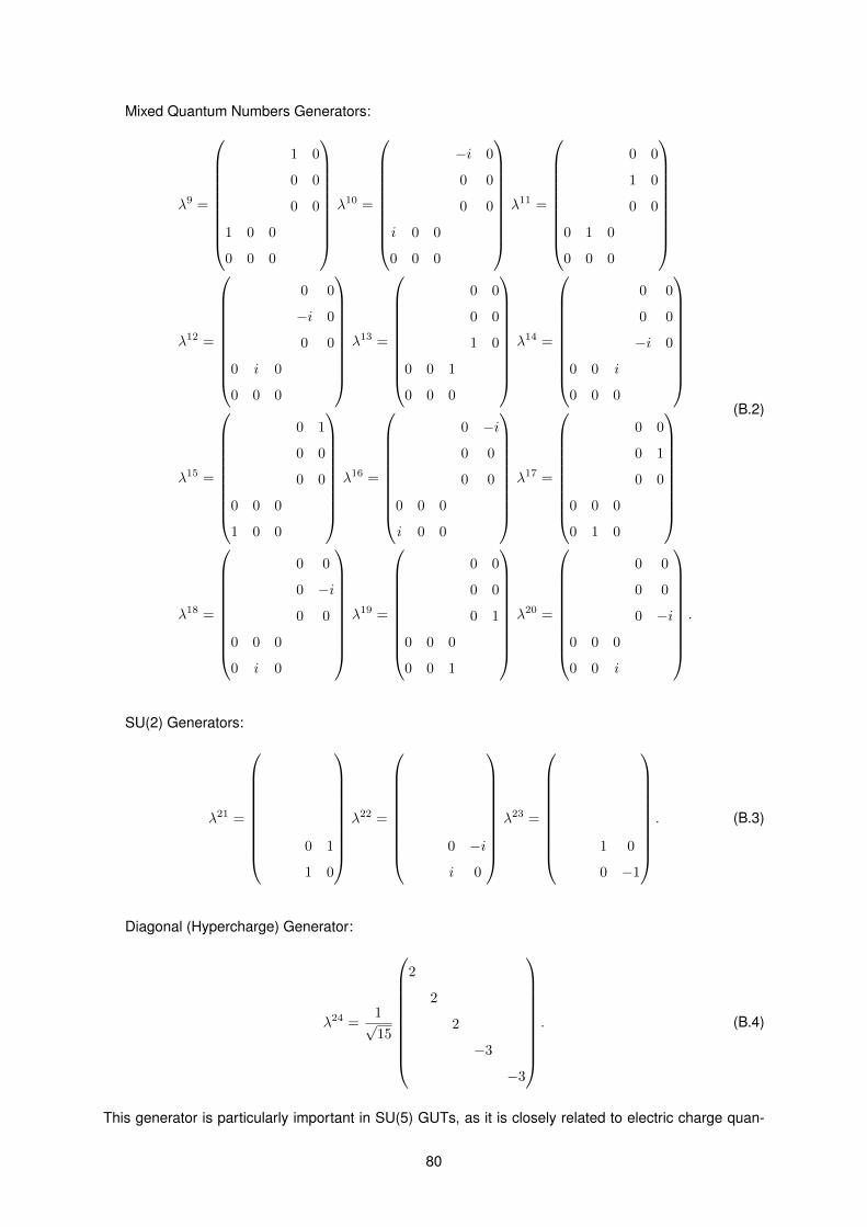
Mixed Quantum Numbers Generators:

λ9 =

1 0

0 0

0 0

1 0 0

0 0 0

λ10 =

−i 0

0 0

0 0

i 0 0

0 0 0

λ11 =

0 0

1 0

0 0

0 1 0

0 0 0

λ12 =

0 0

−i 0

0 0

0 i 0

0 0 0

λ13 =

0 0

0 0

1 0

0 0 1

0 0 0

λ14 =

0 0

0 0

−i 0

0 0 i

0 0 0

λ15 =

0 1

0 0

0 0

0 0 0

1 0 0

λ16 =

0 −i

0 0

0 0

0 0 0

i 0 0

λ17 =

0 0

0 1

0 0

0 0 0

0 1 0

λ18 =

0 0

0 −i

0 0

0 0 0

0 i 0

λ19 =

0 0

0 0

0 1

0 0 0

0 0 1

λ20 =

0 0

0 0

0 −i

0 0 0

0 0 i

.

(B.2)

SU(2) Generators:

λ21 =

0 1

1 0

λ22 =

0 −i

i 0

λ23 =

1 0

0 −1

. (B.3)

Diagonal (Hypercharge) Generator:

λ24 =1√15

2

2

2

−3

−3

. (B.4)

This generator is particularly important in SU(5) GUTs, as it is closely related to electric charge quan-

80

tization. In fact, it has a different eigenvalue for the SU(3) and SU(2) Cartan subalgebras and, after

being multiplied by a normalization factor, it returns the field’s SM hypercharges, so, considering the

definition of electric charge in Chapter 1, charge quantization is achieved (recall that hypercharges were

not determined by gauge group factors in the SM).

B.2 Matter and Higgs Representations

In this section we use the following notation: greek indexes correspond to SU(5), so α, β, γ = 1, ..., 5, the

a, b, c, d= 1, 2, 3 are SU(3) indexes, the r, s, t= 4, 5 are SU(2) indexes, σI represent the Pauli matrices

and λA represent Gell-Mann matrices.

In terms of GSM quantum numbers, the fermionic fields in the Adjoint SU(5) model decompose as

5∗ = dC ⊕ L,

10 = Q⊕ uC ⊕ eC ,

24 = ρ8 ⊕ ρ3 ⊕ ρ(3,2)− 12

⊕ ρ(3∗,2) 12

⊕ ρ0.

(B.5)

Considering this, we may write

5∗a = (dC)a, 5∗r = εrsL2, (B.6)

10ab =1√2εabc(uC)c, 10ar =

1√2Qar, 10rs =

1√2εrseC . (B.7)

Taking into account the fact that

ραβ = ρβ∗α ,∑α=1

5ραα = 0, (B.8)

we get

ρab =1

2ρA8[λA]ab

+

√1

15δab ρ0,

rhoar =[ρ(3,2)

]ar,

ρrs =1

2ρI3[σI]rs−√

3

20δrsρ0.

(B.9)

Proceeding in the same way for the model’s scalars we obtain

5H = T1 ⊕H1,

24H = Σ8 ⊕ Σ3 ⊕ Σ(3,2)− 12

⊕ Σ(3∗,2) 12

⊕ Σ0,

45H = S(8,2) 310

⊕ S(6∗,1)− 15

⊕ S(3∗,2)− 710

⊕ S(3∗,1) 45

⊕∆⊕ T2 ⊕H2,

(B.10)

where ∆ ∼ (3, 3,−1/5). The Hs and Ts are Higgs doublets and coloured triplets, respectively. As for the

81

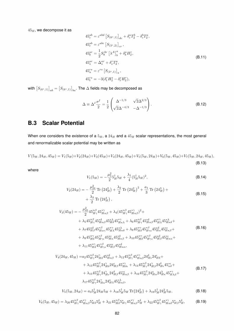
45H , we decompose it as

45abc = εabd[S(6∗,1)

]dc

+ δacTb2 − δbcT a2 ,

45abr = εabc[S(3∗,2)

]cr,

45arb =1

2SAr8

[λA]ab

+ δabHr2 ,

45ars = ∆ars + δrsT

a2 ,

45rsa = εrs[S(3∗,1)

]a,

45rst = −3(δrtHs2 − δstHr

2 ),

(B.11)

with[S(6∗,1)

]ab

=[S(6∗,1)

]ba

. The ∆ fields may be decomposed as

∆ ≡ ∆I σI

2=

1

2

∆−1/3√

2∆2/3

√2∆−4/3 −∆−1/3

. (B.12)

B.3 Scalar Potential

When one considers the existence of a 5H , a 24H and a 45H scalar representations, the most general

and renormalizable scalar potential may be written as

V (5H , 24H , 45H) = V1(5H)+V2(24H)+V3(45H)+V4(24H , 45H)+V5(5H , 24H)+V6(5H , 45H)+V7(5H , 24H , 45H),

(B.13)

where

V1(5H) = −µ25

25†H5H +

λ1

4(5†H5H)2, (B.14)

V2(24H) =− µ224

2Tr(242H

)+λ2

2Tr(242H

)2+a1

3Tr(243H

)+

+λ3

2Tr(244H

),

(B.15)

V3(45H) =− µ245

245αβHγ45∗γHαβ + λ4(45αβHγ45∗γHαβ)2+

+ λ545αβHγ45∗δHαβ45κλHδ45∗γHκλ + λ645αβHγ45∗δHαβ45κγHλ45∗λHκδ+

+ λ745αδHβ45∗βHαγ45κγHλ45∗λHκδ + λ845αγHδ45∗βHγε45κδHα45∗εHκβ+

+ λ945αγHδ45∗βHγε45κεHα45∗δHκβ + λ1045αγHδ45∗βHγε45κδHβ45∗εHκα+

+ λ1145αγHδ45∗βHγε45κεHβ45∗δHκα,

(B.16)

V4(24H , 45H) =a245αβHγ24γHδ45∗δHαβ + λ1245αβHγ45∗γHαβ24δHε24εHδ+

+ λ1345αβHγ24γHδ24εHβ45∗γHδε + λ1445αβHγ24γHβ24δHε45∗εαδ+

+ λ1545αβHγ24γHε24δHβ45∗εHαβ + λ1645αβHγ24κHα24λHκ45∗γHλβ+

λ1745αβHγ24γHκ24κHλ45∗λHαβ ,

(B.17)

V5(5H , 24H) = a35†H24H5H + λ185†H5H Tr{242H}+ λ195†H242

H5H , (B.18)

V6(5H , 45H) = λ2045αβHγ45∗γHαβ5∗Hδ5δH + λ2145αβHδ5

∗Hγ45∗γHαβ5δH + λ2245αβHγ45∗γHαδ5

∗Hβ5δH , (B.19)

82

and

V7(5H , 24H , 45H) = a45∗Hα45αβHδ24δHβ + λ235∗Hα45αβHδ24γHbeta24δHγ +H.c., (B.20)

where the λis and aj are constants.

83

84

Appendix C

Discrete Symmetries that suppress

Proton Decay and resulting Mass

Matrices

In this Appendix we present the different solutions (as far as the Mu and Md mass matrices are con-

cerned) with no tree-level scalar-mediated proton decay, that may be achieved for specific discrete sym-

metries. We also show the case where the new symmetry is continuous (U(1)) to make it clear that some

solutions can only be achieved through discrete symmetries. The row where a given solution is situated

indicates the number of zeros in Mu and the column indicates the number of zeros in Md. Elements

can be null if there is no charge assignment for which there is a solution and Mu, Md have the specified

amount of zeros or a non-null number that represents the possible different solutions with the specified

amount of mass matrix zeros where the textures and the symmetries displayed by the Yukawa matrices

at GUT scale are taken into account.

Z2

0 1 2 3 4 5 6

0 4 0 0 0 0 0 0

1 0 0 0 0 0 0 0

2 0 0 0 0 0 0 0

3 0 0 0 0 0 0 0

4 0 0 0 0 0 0 0

5 0 0 0 0 0 0 0

6 0 0 0 0 0 0 0

Z3

85

0 1 2 3 4 5 6

0 0 0 0 0 0 0 0

1 4 6 12 0 3 0 0

2 0 0 0 0 0 0 0

3 0 0 0 42 0 0 0

4 2 6 12 12 12 0 0

5 0 0 0 0 0 0 0

6 0 0 0 0 0 0 6

Z4

0 1 2 3 4 5 6

0 4 0 0 0 0 0 0

1 4 6 12 0 3 0 0

2 0 0 0 0 0 0 0

3 0 0 0 0 0 0 0

4 0 0 0 42 138 54 0

5 0 0 0 30 105 78 0

6 0 0 0 0 0 0 6

Z5

0 1 2 3 4 5 6

0 0 0 0 0 0 0 0

1 4 6 12 0 3 0 0

2 0 0 0 0 0 0 0

3 0 0 0 0 0 0 0

4 0 0 0 42 111 54 0

5 0 0 0 0 27 84 42

6 0 0 0 0 24 96 42

C.1 Results for ZN × ZM symmetries

Z2 × Z2

0 1 2 3 4 5 6

0 4 0 0 0 0 0 0

1 0 0 0 0 0 0 0

2 0 0 0 0 0 0 0

3 0 0 0 0 0 0 0

4 0 0 0 0 27 0 0

5 0 0 0 0 0 0 0

6 0 0 0 0 0 0 0

86

Z2 × Z3

0 1 2 3 4 5 6

0 4 0 0 0 0 0 0

1 4 6 12 0 3 0 0

2 0 0 0 0 0 0 0

3 0 0 0 42 0 0 0

4 2 6 12 54 123 54 0

5 0 0 0 0 54 168 84

6 0 0 0 0 45 174 108

Z2 × Z4

0 1 2 3 4 5 6

0 4 0 0 0 0 0 0

1 4 6 12 0 3 0 0

2 0 0 0 0 0 0 0

3 0 0 0 0 0 0 0

4 0 0 0 42 153 54 0

5 0 0 0 30 105 120 42

6 0 0 0 0 0 0 126

Z3 × Z3

0 1 2 3 4 5 6

0 0 0 0 0 0 0 0

1 4 6 12 0 3 0 0

2 0 0 0 0 0 0 0

3 0 0 0 42 0 0 0

4 2 6 12 12 12 0 0

5 0 0 0 0 0 0 0

6 0 0 0 0 0 0 78

C.2 Results for continuous symmetries

-5 to 5

0 1 2 3 4 5 6

0 0 0 0 0 0 0 0

1 4 6 12 0 3 0 0

2 0 0 0 0 0 0 0

3 0 0 0 0 0 0 0

4 0 0 0 42 111 54 0

5 0 0 0 0 27 84 42

6 0 0 0 0 24 96 78

87

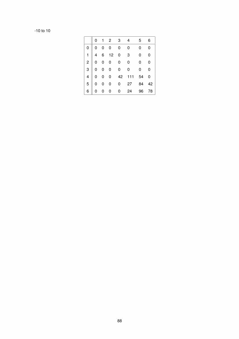
-10 to 10

0 1 2 3 4 5 6

0 0 0 0 0 0 0 0

1 4 6 12 0 3 0 0

2 0 0 0 0 0 0 0

3 0 0 0 0 0 0 0

4 0 0 0 42 111 54 0

5 0 0 0 0 27 84 42

6 0 0 0 0 24 96 78

88