This journal is© the Owner Societies 2016 Phys. Chem. Chem. Phys., 2016, 18, 8545--8553 | 8545

Cite this:Phys.Chem.Chem.Phys.,

2016, 18, 8545

Director orientations in lyotropic liquid crystals:diffusion MRI mapping of the Saupe order tensor

Daniel Topgaard

The macroscopic physical properties of a liquid crystalline material depend on both the properties of the

individual crystallites and the details of their spatial arrangement. We propose a diffusion MRI method to

estimate the director orientations of a lyotropic liquid crystal as a spatially resolved field of Saupe order

tensors. The method relies on varying the shape of the diffusion-encoding tensor to disentangle the effects

of voxel-scale director orientational order and the local diffusion anisotropy of the solvent. Proof-of-concept

experiments are performed on water in lamellar and reverse hexagonal liquid crystalline systems with intricate

patterns of director orientations.

Introduction

Anisotropic assemblies of amphiphilic molecules in aqueousmedia occur in a wide range of materials: from lyotropic liquidcrystals1–3 to brain tissue.4 Locally, the amphiphiles have apreferred orientation with respect to a unit vector known as thedirector,5 and a liquid crystalline domain can be defined as aregion of space in which the director has a constant orienta-tion. Material properties, such as optical birefringence, electri-cal conductivity, and molecular diffusivity, are determined bythe local properties within a single domain as well as the spatialpattern of director orientations, the latter being possible toinfluence by temperature cycling, shear, magnetic fields, or thepresence of solid surfaces.6–27 For technical applications ofliquid crystals in drug delivery28,29 or templating of inorganicmaterials,30,31 it is desirable to control the domain sizes andorientations.

The orientational order of an ensemble of unit vectors isoften expressed as the Saupe order tensor S with elementsSij defined by5,32–34

Sij ¼1

23lilj � kij� �

; (1)

where i,j A {x,y,z}, h�i denotes an ensemble average, kij is theKronecker delta, and li are the directional cosines of the vectorsin the lab frame xyz. The order tensor contains five indepen-dent elements and is often parameterized with the principalorder parameter SZZ, the asymmetry parameter Z, and threeEuler angles describing the orientation of the principal axissystem XYZ with respect to the lab frame. In the Landau–deGennes theory of nematic liquid crystals,5,34 and its extension

to lyotropic nematic liquid crystals,35,36 the free energy densityat the position r is determined by the local order tensor S(r).Hence, the results of mean-field calculations of the structure ofliquid crystals are often visualized as spatially resolved fieldsof order tensors.37–39 An experimental method capable ofmapping such tensor fields would enable critical testing ofthe results of theoretical calculations and allow for detailedcharacterization of liquid crystals for technical applications.

The structure of a lyotropic liquid crystal is imprinted in theorientational order and translational diffusion of the waterlocated in the nanometer-scale gaps between the amphiphileaggregates. The orientational order of the water can be detectedwith 2H nuclear magnetic resonance (NMR) spectroscopy as aquadrupolar splitting of the 2H2O resonance line,40–42 while thestructural anisotropy of the liquid crystal gives rise to a directionaldependence of the water self-diffusion coefficient as observedwith diffusion NMR13,43–48 and magnetic resonance imaging(MRI).24,27,49,50 Despite the fact that these NMR and MRI methodshave been extensively used for investigating macroscopic domainalignment in liquid crystals,8,9,14,15,18,19,21,23,24,26,27,40,44,49–55

there are so far no reported studies where the full order tensorhas been mapped with spatial resolution. In principle, suchtensor maps could be obtained by acquiring spatially resolved2H spectra24,27,55–57 for multiple orientations of the mainmagnetic field.58 Unfortunately, such an experimental approachwould require combinations of NMR hardware that are exceed-ingly rare.

Here, we introduce a diffusion MRI method for mappingdirector order tensors in lyotropic liquid crystals. The newmethod builds on conventional diffusion tensor imaging (DTI),59

which yields the average diffusion tensor hDi for each spatiallyresolved volume element, ‘‘voxel’’, of the image, and our recentmethod for quantifying the microscopic diffusion tensor D withina single liquid crystalline domain of a polydomain sample.60

Division of Physical Chemistry, Department of Chemistry, Lund University, Lund,

Sweden. E-mail: daniel.topgaard@fkem1.lu.se

Received 24th November 2015,Accepted 24th February 2016

DOI: 10.1039/c5cp07251d

www.rsc.org/pccp

PCCP

PAPER

Ope

n A

cces

s A

rtic

le. P

ublis

hed

on 0

7 M

arch

201

6. D

ownl

oade

d on

1/2

5/20

22 7

:03:

47 P

M.

Thi

s ar

ticle

is li

cens

ed u

nder

a C

reat

ive

Com

mon

s A

ttrib

utio

n-N

onC

omm

erci

al 3

.0 U

npor

ted

Lic

ence

.

View Article OnlineView Journal | View Issue

8546 | Phys. Chem. Chem. Phys., 2016, 18, 8545--8553 This journal is© the Owner Societies 2016

The latter method relies on an acquisition protocol wherein notonly the magnitude and direction of the diffusion-encodingis varied, as in conventional DTI, but also the shape of theaxisymmetric diffusion-encoding tensor b.60–64 In the theorysection, we present a detailed derivation of the relation betweenthe tensors hDi, D, and S, parts of which have previouslyappeared in the literature,27,50,65–69 and describe how ordertensor fields can be calculated from independently measuredmaps of hDi and D. We demonstrate the new method by proof-of-principle experiments on lamellar and reverse hexagonallyotropic liquid crystals with a range of director orientationdistributions. The experiments are carried out with a slightlymodified version of the diffusion MRI pulse sequence introducedby Lasic et al.50 and subsequently used for human in vivo studiesin a series of recent publications.62,64,69 We also elaborate on theprocedure for generating axisymmetric diffusion-encoding withsmoothly modulated waveforms for the time-dependent mag-netic field gradients.70

Theoretical considerations

The theory section includes derivations of the expressions forestimating the tensors hDi, D, and S from experimental data, as wellas a summary of the principles of axisymmetric diffusion-encoding

as recently introduced by Eriksson et al.60 Readers mainly interestedin the experimental demonstration of the new approach may wishto go directly to the Results and discussion section, and simplynote that the key equations for data evaluation can be found ineqn (12), (19), and (29).

Diffusion and order tensors

In its principal axis system (PAS), a microscopic diffusiontensor D can be written as

DPAS ¼

DXX 0 0

0 DYY 0

0 0 DZZ

0BBB@

1CCCA; (2)

with the eigenvalues ordered as (DZZ � Diso) Z (DXX � Diso) Z(DYY � Diso), where Diso is the isotropic average of theeigenvalues:

Diso ¼1

3DXX þDYY þDZZð Þ: (3)

Defining the diffusion tensor anisotropy DD and asymmetryDZ as44,60,67

DD ¼1

3DisoDZZ �

DYY þDXX

2

� �and DZ ¼

DYY �DXX

2DisoDD; (4)

Eqn (2) can be rewritten as

DPAS ¼ Diso

1 0 0

0 1 0

0 0 1

0BBB@

1CCCA

8>>><>>>:

þDD

�1 0 0

0 �1 0

0 0 2

0BBB@

1CCCAþDZ

�1 0 0

0 1 0

0 0 0

0BBB@

1CCCA

26664

37775

9>>>=>>>;;

(5)

which is reduced to

DPAS ¼ Diso Iþ 2DD

�1=2 0 0

0 �1=2 0

0 0 1

0BBB@

1CCCA

26664

37775 (6)

if the diffusion tensor is axisymmetric (DZ = 0). In eqn (6), I isthe identity matrix. While Diso corresponds to the ‘‘size’’ of thetensor, the value of DD reports on its ‘‘shape’’, covering therange from �1/2 (planar) to 0 (spherical) and +1 (linear).60

If the eigenframe XYZ of the axisymmetric tensor DPAS isinitially aligned with the lab frame xyz, rotation through thepolar and azimuthal angles y and f yields a lab-frame tensor Dgiven by

Replacing the trigonometric expressions in eqn (7) with thedirectional cosines

lx = cosf sin y

ly = sinf sin y

lz = cos y (8)

gives

D ¼ Diso Iþ 2DD �1

2

3lx2 � 1 3lxly 3lxlz

3lxly 3ly2 � 1 3lylz

3lxlz 3lylz 3lz2 � 1

0BBB@

1CCCA

26664

37775: (9)

The terms with directional cosines can be recognized from thedefinition of the Saupe order tensor S in eqn (1), which inmatrix form can be written as

S ¼ 1

2

3lx2 � 1

� �3lxly� �

3lxlzh i

3lxly� �

3ly2 � 1

� �3lylz� �

3lxlzh i 3lylz� �

3lz2 � 1

� �

0BBB@

1CCCA: (10)

The principal order parameter SZZ is defined as the eigenvalueof S with the largest magnitude.33 The values of SZZ cover therange from �1/2 to +1. Perfect alignment in a single direction

D ¼ Diso Iþ 2DD �1

2

3 cos2 f sin2 y� 1 3 sinf cosf sin2 y 3 cosf sin y cos y

3 sinf cosf sin2 y 3 sin2 f sin2 y� 1 3 sinf sin y cos y

3 cosf sin y cos y 3 sinf sin y cos y 3 cos2 y� 1

0BBB@

1CCCA

26664

37775: (7)

Paper PCCP

Ope

n A

cces

s A

rtic

le. P

ublis

hed

on 0

7 M

arch

201

6. D

ownl

oade

d on

1/2

5/20

22 7

:03:

47 P

M.

Thi

s ar

ticle

is li

cens

ed u

nder

a C

reat

ive

Com

mon

s A

ttrib

utio

n-N

onC

omm

erci

al 3

.0 U

npor

ted

Lic

ence

.View Article Online

This journal is© the Owner Societies 2016 Phys. Chem. Chem. Phys., 2016, 18, 8545--8553 | 8547

corresponds to SZZ = 1, while random orientations in a planeperpendicular to the director gives SZZ = �1/2. The value SZZ = 0indicates completely random orientations in 3D space, butcould also result from other, more exotic, orientation distribu-tions, e.g., three orthogonal directions with equal probability orrandom orientations on a cone with aperture 109.41.

Assuming that there is no molecular exchange between thedomains on the 10–100 ms time-scale defined by the diffusionNMR experiment, then hDi is simply the population-weightedaverage of the domain tensors D.65 For an ensemble of tensorswith the same size Diso and shape DD, but different orientations(y,f), application of ensemble averaging to both sides of eqn (9)yields

hDi = Diso(I + 2DDS), (11)

where hDi is the ensemble-average or ‘‘voxel-average’’ diffusiontensor as measured with standard DTI.59 Quantitative estimatesof Diso and DD can be obtained with the method of axisymmetricdiffusion-encoding introduced by Eriksson et al.60 and describedbelow. Once hDi, Diso and DD have been determined, S can becalculated through element-by-element inversion of eqn (11):

Sij ¼1

2DD�

Dij

� �Diso

� kij

� �: (12)

From eqn (11) follows that the anisotropy lD of the averagetensor hDi is given by67

lD = SZZDD. (13)

Maximal macroscopic anisotropy (lD = 1) requires that both themicroscopic anisotropy DD and the principal order parameterSZZ equal 1. Conversely, a planar macroscopic tensor (lD =�1/2)could result from either perfect alignment of planar microscopictensors (SZZ = 1, DD = �1/2) or negative uniaxial alignment oflinear microscopic tensors (SZZ = �1/2, DD = 1).

Diffusion tensors are often visualized as ellipsoid59 or super-quadric71 tensor glyphs, where the lengths and directions of thethree semi-axes are given by the corresponding tensor eigen-values and eigenvectors. According to the definition in eqn (1),the tensor S is traceless and has both positive and negativeeigenvalues, which cannot directly be represented as the con-ventional tensor glyphs. Various approaches for manipulatingthe order tensor to facilitate visualization can be found inthe literature.37–39 Here, we define a shifted and rescaled ordertensor S0 through

S0 ¼ 1

3ðIþ 2SÞ: (14)

The eigenvalues of the symmetric and unit-trace tensor S0 areall positive, covering the range from 0 to 1, and the eigenvectorscoincide with the ones for hDi. Consequently, the S0 and hDitensor fields can be visualized using the same kind of glyphs orcolor-code.

NMR diffusion-encoding

The NMR signal is encoded with information about transla-tional motion by applying a time-dependent magnetic field

gradient G(t) in the time interval 0 r t r t. The diffusion-encoding tensor b is given by72,73

b ¼ðt0

qðtÞqTðtÞdt; (15)

where

qðtÞ ¼ gðt0

Gðt 0Þdt 0 (16)

is the time-dependent dephasing vector and g is the magneto-gyric ratio of the studied nucleus. The gradient waveform G(t)obeys the ‘‘echo condition’’ q(t) = 0.

For a sample or volume element comprising an ensembleof microscopic diffusion tensors D, the NMR signal I(b) can bewritten as72,73

I(b) = I0hexp(�b:D)i (17)

where I0 is the signal when b = 0 and b:D is a generalized scalarproduct defined as

b:D ¼Xi

Xj

bijDij : (18)

In the limit b - 0, eqn (19) can be approximated as64

I(b) = I0 exp(�b:hDi), (19)

where hDi is the ensemble-average diffusion tensor. Eqn (19) corre-sponds to the conventional equation for evaluating DTI data.72,73

Parameterization of the b-tensor

In analogy with the description of the diffusion tensor above,the b-tensor can, in its principal axis system, be expressed as

bPAS ¼

bXX 0 0

0 bYY 0

0 0 bZZ

0BBB@

1CCCA; (20)

where the eigenvalues are ordered according to the convention(bZZ � b/3) Z (bXX � b/3) Z (bYY � b/3), and b is the trace of theb-tensor:

b = bXX + bYY + bZZ. (21)

The b-tensor anisotropy bD and asymmetry bZ are given by60

bD ¼1

bbZZ �

bYY þ bXX

2

� �and bZ ¼

3

2� bYY � bXX

bbD: (22)

With the parameterization in eqn (21) and (22), eqn (20) can berecast into

bPAS ¼ b

3

1 0 0

0 1 0

0 0 1

0BBB@

1CCCA

8>>><>>>:

þ bD

�1 0 0

0 �1 0

0 0 2

0BBB@

1CCCAþ bZ

�1 0 0

0 1 0

0 0 0

0BBB@

1CCCA

26664

37775

9>>>=>>>;:

(23)

PCCP Paper

Ope

n A

cces

s A

rtic

le. P

ublis

hed

on 0

7 M

arch

201

6. D

ownl

oade

d on

1/2

5/20

22 7

:03:

47 P

M.

Thi

s ar

ticle

is li

cens

ed u

nder

a C

reat

ive

Com

mon

s A

ttrib

utio

n-N

onC

omm

erci

al 3

.0 U

npor

ted

Lic

ence

.View Article Online

8548 | Phys. Chem. Chem. Phys., 2016, 18, 8545--8553 This journal is© the Owner Societies 2016

Axisymmetric diffusion-encoding corresponds to bZ = 0, and asimplified expression for the b-tensor can be written as

bPAS ¼ b

3Iþ 2bD

�1=2 0 0

0 �1=2 0

0 0 1

0BBB@

1CCCA

26664

37775: (24)

For an axisymmetric b-tensor initially aligned with the lab frame,rotation through the polar and azimuthal angles Y and F givesthe lab-frame b-tensor

Powder-averaged signal

Inserting the expressions for the axisymmetric tensors b andD in eqn (7) and (25), respectively, into eqn (18) yields

b:D = bDiso[1 + 2bDDDP2(cos b)], (26)

where

cos b = cosY cos y + sinY sin y cos(F � f), (27)

and P2(x) = (3x2 � 1)/2 is the 2nd Legendre polynomial. Forsamples comprising randomly oriented microscopic domains,or when powder-averaged signal acquisition is applied,50 theprobability distribution P(b) of the angle b is given by

PðbÞ ¼ 1

2sinb (28)

in the interval 0 r b r 1801. Using eqn (26) and (28) whenevaluating the ensemble average in eqn (17) yields60

I b; bDð Þ ¼ I0 exp �bDisoð Þ

�ffiffiffipp

2

exp bDisobDDDð Þerfffiffiffiffiffiffiffiffiffiffiffiffiffiffiffiffiffiffiffiffiffiffiffiffi3bDisobDDDp� �

ffiffiffiffiffiffiffiffiffiffiffiffiffiffiffiffiffiffiffiffiffiffiffiffi3bDisobDDDp ;

(29)

where erf(x) is the error function. Eqn (29) can be used toextract values of Diso and DD by analyzing the powder-averagedsignal I(b,bD) acquired as a function of b and bD.60

Gradient waveforms for axisymmetric diffusion-encoding

An axially symmetric b-tensor can be obtained by selecting aq-vector trajectory

qðtÞ ¼

qX ðtÞ

qY ðtÞ

qZðtÞ

26664

37775 ¼ qðtÞ

cos½cðtÞ� sinðzÞ

sin½cðtÞ� sinðzÞ

cosðzÞ

26664

37775; (30)

where the q-vector magnitude q(t) and azimuthal angle c(t)satisfy the relation70,74

cðtÞ ¼ 2pb

ðt0

qðtÞ2dt; (31)

and the polar angle z is constant. In eqn (31), b is the trace ofthe b-tensor, which can be calculated with eqn (15) and (20), or,alternatively, directly from q(t) using75

b ¼ðt0

qðtÞ2dt: (32)

The angle z determines the b-tensor anisotropy bD according to60

bD = P2(cos z), (33)

where P2(x) is the 2nd Legendre polynomial as defined beloweqn (27). The gradient G(t) is given by the derivative

GðtÞ ¼ 1

g� ddtqðtÞ: (34)

Explicit gradient waveforms obeying the constraints abovecan be constructed by selecting an axial waveform GA(t)from a standard pulsed gradient spin echo experiment with,e.g., rectangular, ramped, sinusoidal, Gaussian, or exponentialgradient pulse shapes.76,77 The chosen waveform then givesq(t) from

qðtÞ ¼ gðt0

GAðt 0Þdt 0 (35)

and b and c(t) with eqn (31) and (32), respectively. Inserting q(t)and c(t) into eqn (30) and (34) yields

GðtÞ ¼

GXðtÞ

GY ðtÞ

GZðtÞ

26664

37775 ¼

Re GRðtÞ½ � sinðzÞ

Im GRðtÞ½ � sinðzÞ

GAðtÞ cosðzÞ

26664

37775; (36)

where GR(t) is the complex radial gradient waveform

GRðtÞ ¼ GAðtÞ þ2pqðtÞ3

gbi

exp½icðtÞ�: (37)

As shown in Fig. 1(a), axisymmetric diffusion-encoding canbe implemented in a diffusion MRI pulse sequence by replacingthe conventional rectangular or ramped gradient pulses withthe waveform G(t).50,62,64,69 The procedure for transforming anaxial waveform GA(t) and a value of z to G(t) is summarized inFig. 1(b). First, GA(t) is converted to q(t), b, and c(t) usingeqn (31), (32), and (35), respectively. Subsequently, thesefunctions and values give the radial waveform GR(t) viaeqn (37). Finally, G(t) is obtained by combining GA(t) andGR(t) with amplitude scaling given by the angle z as describedin eqn (36). Under the condition that the XYZ PAS of thegradients is initially aligned with the xyz lab frame, rotationof G(t) through the angles (Y,F) yields b-tensor elementsaccording to eqn (25) with b and bD being given by GA(t) andz via eqn (32), (33), and (35).

b ¼ b

3Iþ bD

3 cos2 F sin2 Y� 1 3 sinF cosF sin2 Y 3 cosF sinY cosY

3 sinF cosF sin2 Y 3 sin2 F sin2 Y� 1 3 sinF sinY cosY

3 cosF sinY cosY 3 sinF sinY cosY 3 cos2 Y� 1

0BBB@

1CCCA

26664

37775: (25)

Paper PCCP

Ope

n A

cces

s A

rtic

le. P

ublis

hed

on 0

7 M

arch

201

6. D

ownl

oade

d on

1/2

5/20

22 7

:03:

47 P

M.

Thi

s ar

ticle

is li

cens

ed u

nder

a C

reat

ive

Com

mon

s A

ttrib

utio

n-N

onC

omm

erci

al 3

.0 U

npor

ted

Lic

ence

.View Article Online

This journal is© the Owner Societies 2016 Phys. Chem. Chem. Phys., 2016, 18, 8545--8553 | 8549

ExperimentalSample preparation

The nonionic surfactant penta(ethylene glycol) monotetradecylether (C14E5) forms a lamellar phase (La) in water over a widerange of concentrations and temperatures.25 The planar geo-metry of the water compartments in the La phase gives rise to acorrespondingly planar shape of the microscopic diffusion tensorand a value of DD approaching �1/2.60 The phase diagram ofsodium 1,4-bis(2-ethylhexoxy)-1,4-dioxobutane-2-sulfonate (AOT)/2,2,4-trimethylpentane (isooctane)/water is dominated by areverse hexagonal phase (HII) at 25 1C.2 The nearly linear shapeof the water compartments in the HII phase is mirrored in thelinear shape of the microscopic diffusion tensors and values ofDD near +1.60,63

The liquid crystals were made with water containing 90 wt%1H2O (Milli-Q quality) and 10 wt% 2H2O (99.8 mol% 2H, ArmarChemicals, Switzerland) in order to allow for NMR observationof both 1H and 2H nuclei. All other chemicals were of analyticalgrade and purchased from Sigma-Aldrich, Sweden. The sampleswere prepared by weighing appropriate amounts of the ingredientsinto 10 ml vials, which were sealed by screw caps and centrifugeduntil the mixtures turned homogeneous. Subsequently, 0.5 mlwas transferred to 5 mm disposable NMR tubes, which wereflame sealed and subjected to further centrifugation to removeair bubbles. One C14E5 sample (61.2 wt% surfactant) underwenttemperature cycling within the field of the NMR magnet asdescribed by Bernin et al.27 in order to produce an La phasewith lamellar directors aligned with the surface normals of the

tube walls, while another C14E5 sample (59.7 wt% surfactant)was not exposed to any further treatment after centrifugation ofthe NMR tube. These two samples will be referred to as‘‘oriented La’’ and ‘‘random La’’, respectively. NMR experimentson the C14E5 samples were performed at 50 � 1 1C. TheAOT/isooctane/water samples were melted to reverse micellarphases at 50 1C, and subsequently cooled down at differentrates to produce varying degrees of domain alignment.1,78 Onesample (38 wt% AOT, 14 wt% isooctane) was slowly cooled to20 1C over 12 h, giving domains preferentially aligned perpendicularto the surface normals of the tube walls. The sample was furtherequilibrated at 20 1C for 12 months before the NMR experiments.A second sample (44 wt% AOT, 17 wt% isooctane) was cooled to15 1C in less than 1 min, giving nearly randomly oriented domains,and was immediately investigated with NMR. These samples will bereferred to as ‘‘oriented HII’’ and ‘‘random HII’’, respectively. TheHII samples were studied with NMR at 20 � 1 1C.

NMR experiments

NMR experiments were carried out on a Bruker Avance II500 spectrometer (Bruker, Karlsruhe, Germany) operating at500.13 MHz 1H resonance frequency. The 11.7 T magnet wasequipped with a MIC-5 probe capable of delivering 3 T m�1

magnetic field gradients in three orthogonal directions. Thesample temperature was controlled with a stream of air using aBVT 2000 unit. Diffusion MRI experiments were performed withTopspin 2.1 using the pulse sequence in Fig. 1(a), which isbased on the sequence introduced by Lasic et al.50 The imageswere read out with a rapid acquisition with relaxation enhance-ment (RARE) block,79 giving 4.8 � 4.8 mm field-of-view (x � y),128 � 32 acquisition matrix size, 5 mm slice thickness (z), and65 ms duration of the echo train. The relation between the imagingslice and the NMR tube is shown in Fig. 2. The RARE block was

Fig. 1 Axisymmetric diffusion-encoding in diffusion MRI. (a) Pulse sequencewith a spin echo (901 and 1801 RF pulses) preceding RARE image read-out.Identical diffusion-encoding gradient waveforms G(t) with duration t bracketthe 1801 pulse. The Cartesian components Gx, Gy, and Gz are shown in red,green, and blue, respectively. (b) Flow-scheme for generating G(t). Thepanels show the axial and radial waveforms GA(t) and GR(t), and the magni-tude q(t) and azimuthal angle c(t) of the dephasing vector q(t). The real andimaginary parts of GR(t) are colored red and green, respectively. Themagnitude b and anisotropy bD of the b-tensor are given by GA(t) and theq-vector inclination z via eqn (32), (33) and (35). Rotation of G(t) throughthe polar and azimuthal angles Y and F results in the corresponding rotationof the b-tensor.

Fig. 2 Schematic geometry for the MRI experiments on samples with0.5 ml liquid crystal in an NMR tube with 5 mm outer diameter. The coilsfor generating the magnetic field gradients define the xyz lab frame. Thegray box indicates the 5 mm thick slice excited in the MRI experiments. Themagnified black square shows the 4.8� 4.8 mm field-of-view of the imageplane, while the gray circle delineates the outer surface of the liquid crystalwithin this plane. The tensor glyphs represent voxel-average diffusiontensors hDi for the oriented La sample obtained at 0.3 mm � 0.3 mmresolution in the xy-plane.

PCCP Paper

Ope

n A

cces

s A

rtic

le. P

ublis

hed

on 0

7 M

arch

201

6. D

ownl

oade

d on

1/2

5/20

22 7

:03:

47 P

M.

Thi

s ar

ticle

is li

cens

ed u

nder

a C

reat

ive

Com

mon

s A

ttrib

utio

n-N

onC

omm

erci

al 3

.0 U

npor

ted

Lic

ence

.View Article Online

8550 | Phys. Chem. Chem. Phys., 2016, 18, 8545--8553 This journal is© the Owner Societies 2016

preceded by a spin-echo diffusion-encoding block with 35 msduration. Identical gradient waveforms G(t) of duration t = 15.9 msand maximum gradient amplitude of approximately 1.2 T m�1

were located on each side of the 1801 pulse. A shaped gradientpulse with 1.59 ms quarter-sine ramp-up and 2.39 ms half-cosineramp-down was used to define an axial waveform GA(t), whichwas converted to the radial waveform GR(t) and G(t) as describedwith the scheme in Fig. 1(b). The diffusion-encoding tensor bwas sampled for a grid of four magnitudes b (geometric spacingfrom 26 to 8610 � 106 s m�2), four anisotropies bD (linearspacing from �0.5 to 1), and 31 directions (Y,F) chosenaccording to the electrostatic repulsion scheme,80 giving in total496 images. The values of bD and b were varied by changing theangle z and scaling the amplitudes of the waveforms GA(t) andGR(t) at constant timing parameters. Each image was acquired asthe sum of two transients at 3 s recycle delay, resulting in 52 minof total experiment time.

Data analysis

All data processing was performed with in-house code writtenin Matlab (MathWorks, Natick, MA). The images were recon-structed at 128 � 128 matrix size, giving 37.5 mm � 37.5 mmnominal spatial resolution, and subjected to 0.15 mm Gaussiansmoothing. For each voxel, the average diffusion tensor hDi wasevaluated by non-linear fitting of eqn (19) to the acquired signal

intensities I(b),72,73 using the initial intensity I0 and the threeeigenvalues and Euler angles of hDi as adjustable parameters.Equations for evaluating the tensor elements hDiji from theeigenvalues and Euler angles can be found in, e.g., the tutorialby Kingsley,81 while eqn (25) gives the relations between the btensor elements and its parameterization as b, bD, Y, and F.The sizes and shapes of the microscopic diffusion tensors Dwere estimated on a voxel-by-voxel basis by averaging the I(b)data over the 31 acquisition directions,50 leaving a reduced setof 4 � 4 data points I(b,bD), and fitting eqn (29) to the datausing I0, Diso, and DD as adjustable parameters.60 Subsequently,the elements of the Saupe order tensor S were evaluated byinserting the values of hDiji, Diso, and DD into eqn (12). Thefit results were downsampled to 16 � 16 matrix size, corres-ponding to 0.3 mm � 0.3 mm spatial resolution, when dis-playing the results as superquadric tensor glyphs,71 while the128 � 128 matrix size was used for generating color-codedparameter maps.

Results and discussion

Experimental tensors hDi, D, and S0 are shown in Fig. 3 forall samples. The oriented La sample features oblate (lD o 0)tensors hDi with minor axes in parallel with the normal vectorsof the tube wall. The nearly planar shape (lD =�1/2) is consistent

Fig. 3 Experimental results for the oriented La (row 1), random La (row 2), oriented HII (row 3), and random HII (row 4) samples displayed as superquadrictensor glyphs representing the voxel-average diffusion tensor hDi (column 1), microscopic diffusion tensor D (column 2), and order tensor S0 (column 3)at a spatial resolution of 0.3 mm � 0.3 mm in the xy-plane. The figures show an oblique view of a section of the image plane illustrated in Fig. 2. Theexperiment for determining D is designed to be insensitive to tensor orientation, and, for simplicity, all these tensors are shown with the cylindricalsymmetry axis along the z-direction.

Paper PCCP

Ope

n A

cces

s A

rtic

le. P

ublis

hed

on 0

7 M

arch

201

6. D

ownl

oade

d on

1/2

5/20

22 7

:03:

47 P

M.

Thi

s ar

ticle

is li

cens

ed u

nder

a C

reat

ive

Com

mon

s A

ttrib

utio

n-N

onC

omm

erci

al 3

.0 U

npor

ted

Lic

ence

.View Article Online

This journal is© the Owner Societies 2016 Phys. Chem. Chem. Phys., 2016, 18, 8545--8553 | 8551

with the underlying lamellar geometry of the liquid crystal, butcould according to eqn (13) in principle result from an ensembleof linear microscopic diffusion tensors (DD = 1) randomly orientedwithin a single plane (SZZ = �1/2). All experimental D are oblatewith values of the DD around�0.49, proving that the liquid crystalis of the lamellar type throughout the sample. Using the knowl-edge of the size and shape of D, information about the directororientations can be disentangled from hDi using eqn (12). Fornearly all voxels of the oriented La sample, the order tensors S0 arelinear (SZZ E 1), indicating a single preferred director orientationwithin each voxel, and oriented radially with respect to the tubeaxis. A few exceptions occur in the very center of the tube, wherethe planar shapes of the S0 tensors show that the voxels contain adistribution of director orientations within the xy-plane.

The hDi tensors for the random La sample have shapes rangingfrom oblate (lD o 0) to prolate (lD 4 0). Since all D tensors areidentical also in this case, the varying shapes of hDi result fromthe voxel-scale orientation distributions rather than from anydifferences in the microscopic geometries of the liquid crystal.The resulting S0 tensors cover a range of shapes, but they are allmainly located within the xy-plane, indicating that the directors inthe ‘‘random’’ La sample tend to avoid the z-direction just as forthe oriented La sample, albeit with a less distinct radial pattern.

The oriented HII sample yields mainly prolate hDi tensors ina pattern forming nearly concentric circles in the image plane,while the random HII sample features hDi tensors covering arange of shapes from oblate to spherical. The corresponding Dtensors all have prolate shapes and values of DD around 0.9,leading to similar shapes and identical semi-axis orientationsof the hDi and S0 tensors. The concentric pattern of hDi tensororientations for the oriented HII sample thus directly correspondsto the pattern of director orientations. The nearly spherical hDiand S0 tensors in the interior of the random HII sample verify thatthe directors to a reasonable approximation are randomlyoriented, while the more oblate tensors close to the glasssurface indicate that director orientations in parallel with thesurface normal vectors are less favorable.

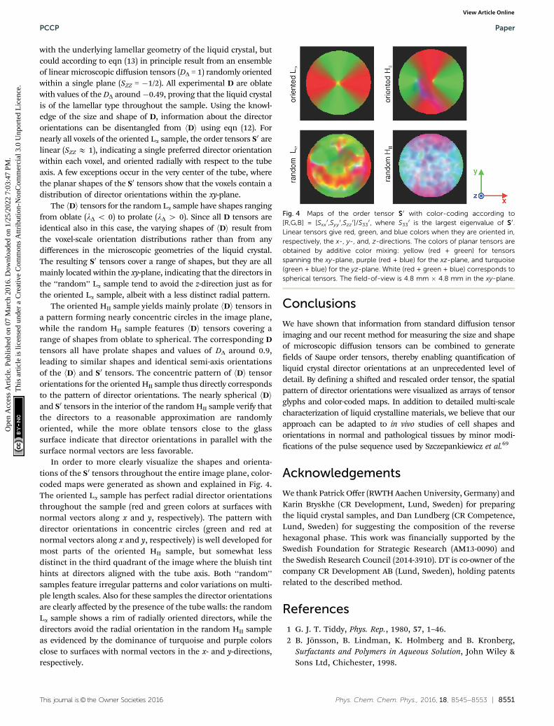
In order to more clearly visualize the shapes and orienta-tions of the S0 tensors throughout the entire image plane, color-coded maps were generated as shown and explained in Fig. 4.The oriented La sample has perfect radial director orientationsthroughout the sample (red and green colors at surfaces withnormal vectors along x and y, respectively). The pattern withdirector orientations in concentric circles (green and red atnormal vectors along x and y, respectively) is well developed formost parts of the oriented HII sample, but somewhat lessdistinct in the third quadrant of the image where the bluish tinthints at directors aligned with the tube axis. Both ‘‘random’’samples feature irregular patterns and color variations on multi-ple length scales. Also for these samples the director orientationsare clearly affected by the presence of the tube walls: the randomLa sample shows a rim of radially oriented directors, while thedirectors avoid the radial orientation in the random HII sampleas evidenced by the dominance of turquoise and purple colorsclose to surfaces with normal vectors in the x- and y-directions,respectively.

Conclusions

We have shown that information from standard diffusion tensorimaging and our recent method for measuring the size and shapeof microscopic diffusion tensors can be combined to generatefields of Saupe order tensors, thereby enabling quantification ofliquid crystal director orientations at an unprecedented level ofdetail. By defining a shifted and rescaled order tensor, the spatialpattern of director orientations were visualized as arrays of tensorglyphs and color-coded maps. In addition to detailed multi-scalecharacterization of liquid crystalline materials, we believe that ourapproach can be adapted to in vivo studies of cell shapes andorientations in normal and pathological tissues by minor modi-fications of the pulse sequence used by Szczepankiewicz et al.69

Acknowledgements

We thank Patrick Offer (RWTH Aachen University, Germany) andKarin Bryskhe (CR Development, Lund, Sweden) for preparingthe liquid crystal samples, and Dan Lundberg (CR Competence,Lund, Sweden) for suggesting the composition of the reversehexagonal phase. This work was financially supported by theSwedish Foundation for Strategic Research (AM13-0090) andthe Swedish Research Council (2014-3910). DT is co-owner of thecompany CR Development AB (Lund, Sweden), holding patentsrelated to the described method.

References

1 G. J. T. Tiddy, Phys. Rep., 1980, 57, 1–46.2 B. Jonsson, B. Lindman, K. Holmberg and B. Kronberg,

Surfactants and Polymers in Aqueous Solution, John Wiley &Sons Ltd, Chichester, 1998.

Fig. 4 Maps of the order tensor S0 with color-coding according to[R,G,B] = [Sxx

0,Syy0,Szz

0]/S330, where S33

0 is the largest eigenvalue of S0.Linear tensors give red, green, and blue colors when they are oriented in,respectively, the x-, y-, and, z-directions. The colors of planar tensors areobtained by additive color mixing: yellow (red + green) for tensorsspanning the xy-plane, purple (red + blue) for the xz-plane, and turquoise(green + blue) for the yz-plane. White (red + green + blue) corresponds tospherical tensors. The field-of-view is 4.8 mm � 4.8 mm in the xy-plane.

PCCP Paper

Ope

n A

cces

s A

rtic

le. P

ublis

hed

on 0

7 M

arch

201

6. D

ownl

oade

d on

1/2

5/20

22 7

:03:

47 P

M.

Thi

s ar

ticle

is li

cens

ed u

nder

a C

reat

ive

Com

mon

s A

ttrib

utio

n-N

onC

omm

erci

al 3

.0 U

npor

ted

Lic

ence

.View Article Online

8552 | Phys. Chem. Chem. Phys., 2016, 18, 8545--8553 This journal is© the Owner Societies 2016

3 D. F. Evans and H. Wennerstrom, The Colloidal Domain:Where Physics, Chemistry, Biology, and Technology Meet,Wiley-VCH, New York, 2nd edn, 1999.

4 C. Beaulieu, NMR Biomed., 2002, 15, 435–455.5 P. G. de Gennes and J. Prost, The Physics of Liquid Crystals,

Clarendon Press, Oxford, 2nd edn, 1995.6 K. G. Gotz and K. Heckmann, J. Colloid Sci., 1958, 13,

266–272.7 K. D. Lawson and T. J. Flautt, J. Am. Chem. Soc., 1969, 89,

5489–5491.8 K. Radley, L. W. Reeves and A. S. Tracey, J. Phys. Chem.,

1976, 80, 174–182.9 B. J. Forrest and L. W. Reeves, Chem. Rev., 1981, 81, 1–14.

10 N. Boden, S. A. Corne and K. W. Jolley, Chem. Phys. Lett.,1984, 105, 99–103.

11 P. J. Photinos and A. Saupe, J. Chem. Phys., 1986, 84,517–521.

12 P. J. Photinos and A. Saupe, J. Chem. Phys., 1986, 85,7467–7471.

13 J. Chung and J. H. Prestegard, J. Phys. Chem., 1993, 97,9837–9843.

14 G. Briganti, A. L. Segre, D. Capitani, C. Casieri and C. LaMesa, J. Phys. Chem. B, 1999, 103, 825–830.

15 D. Capitani, C. Casieri, G. Briganti, C. La Mesa andA. L. Segre, J. Phys. Chem. B, 1999, 103, 6088–6095.

16 T. D. Le, U. Olsson, K. Mortensen, J. Zipfel and W. Richtering,Langmuir, 2001, 17, 999–1008.

17 F. Nettesheim, I. Grillo, P. Lindner and W. Richtering,Langmuir, 2004, 20, 3947–3953.

18 A. Yethiraj, D. Capitani, N. E. Burlinson and E. E. Burnell,Langmuir, 2005, 21, 3311–3321.

19 J. S. Clawson, G. P. Holland and T. M. Alam, Phys. Chem.Chem. Phys., 2006, 8, 2635–2641.

20 Y. Iwashita and H. Tanaka, Nat. Mater., 2006, 5, 147–152.21 D. Capitani, A. Yethiraj and E. E. Burnell, Langmuir, 2007,

23, 3036–3048.22 T. M. Alam and S. K. McIntyre, Langmuir, 2008, 24,

13890–13896.23 B. Medronho, S. Shafei, R. Szopko, M. G. Miguel, U. Olsson

and C. Schmidt, Langmuir, 2008, 24, 6480–6486.24 B. Medronho, J. Brown, M. G. Miguel, C. Schmidt, U. Olsson

and P. Galvosas, Soft Matter, 2011, 7, 4938–4947.25 D. Sato, K. Obara, Y. Kawabata, M. Iwahashi and T. Kato,

Langmuir, 2013, 29, 121–132.26 B. Medronho, U. Olsson, C. Schmidt and P. Galvosas,

Z. Phys. Chem., 2012, 226, 1293–1314.27 D. Bernin, V. Koch, M. Nyden and D. Topgaard, PLoS One,

2014, 9, e98752.28 O. Freund, J. Amedee, D. Roux and R. Laversanne, Life Sci.,

2000, 67, 411–419.29 F. Tiberg and M. Johnsson, J. Drug Delivery Sci. Technol.,

2011, 21, 101–109.30 G. S. Attard, J. C. Glyde and C. G. Goltner, Nature, 1995, 378,

366–368.31 A. Firouzi, D. J. Schaefer, S. H. Tolbert, G. D. Stucky and

B. F. Chmelka, J. Am. Chem. Soc., 1997, 119, 9466–9477.

32 A. Saupe and G. Englert, Phys. Rev. Lett., 1963, 11, 462–464.33 Nuclear Magnetic Resonance of Liquid Crystals, ed. J. W.

Emsley, D. Reidel Publishing Company, Dordrecht, 1985.34 A. D. Rey, Soft Matter, 2010, 6, 3402–3429.35 S. Kumar, J. D. Litster and C. Rosenblatt, Phys. Rev. A: At.,

Mol., Opt. Phys., 1983, 28, 1890–1892.36 R. Moldovan and M. R. Puica, Phys. Lett. A, 2001, 286,

205–209.37 A. Sonnet, A. Kilian and S. Hess, Phys. Rev. E: Stat. Phys.,

Plasmas, Fluids, Relat. Interdiscip. Top., 1995, 52, 718–722.38 T. Tsuji and A. D. Rey, Phys. Rev. E: Stat. Phys., Plasmas,

Fluids, Relat. Interdiscip. Top., 1998, 57, 5609–5625.39 T. J. Jankun-Kelly and K. Mehta, IEEE Trans. Vis. Comput.

Graph., 2006, 12, 1197–1204.40 K. D. Lawson and T. J. Flautt, J. Phys. Chem., 1968, 72,

2066–2074.41 R. Blinc, K. Easwaran, J. Pirs, M. Volfan and I. Zupancic,

Phys. Rev. Lett., 1970, 25, 1327–1330.42 N.-O. Persson, K. Fontell, B. Lindman and G. J. T. Tiddy,

J. Colloid Interface Sci., 1975, 53, 461–466.43 G. J. T. Tiddy, J. Chem. Soc., Faraday Trans. 1, 1977, 73,

1731–1737.44 G. Chidichimo, L. Coppola, C. La Mesa, G. A. Ranieri and

A. Saupe, Chem. Phys. Lett., 1988, 145, 85–89.45 M. C. Holmes, P. Sotta, Y. Hendrikx and B. Deloche, J. Phys.

II, 1993, 3, 1735–1746.46 S. R. Wassall, Biophys. J., 1996, 71, 2724–2732.47 H. Johanneson and B. Halle, J. Chem. Phys., 1996, 104,

6807–6817.48 S. Gaemers and A. Bax, J. Am. Chem. Soc., 2001, 123,

12343–12352.49 K. Szutkowski and S. Jurga, J. Phys. Chem. B, 2010, 114,

165–173.50 S. Lasic, F. Szczepankiewicz, S. Eriksson, M. Nilsson and

D. Topgaard, Front. Phys., 2014, 2, 11.51 S. Funari, M. C. Holmes and G. J. T. Tiddy, J. Phys. Chem.,

1992, 96, 11029–11038.52 P. L. Hubbard, K. M. McGrath and P. T. Callaghan, J. Phys.

Chem. B, 2006, 110, 20781–20788.53 B. Medronho, C. Schmidt, U. Olsson and M. G. Miguel,

Langmuir, 2010, 26, 1477–1481.54 J. R. Brown and P. T. Callaghan, Soft Matter, 2011, 7,

10472–10482.55 P. Trigo-Mourino, C. Merle, M. R. Koos, B. Luy and R. R. Gil,

Chem. – Eur. J., 2013, 19, 7013–7019.56 E. Fischer and P. T. Callaghan, Europhys. Lett., 2000, 50,

803–809.57 S. Bulut, I. Åslund, D. Topgaard, H. Wennerstrom and

U. Olsson, Soft Matter, 2010, 6, 4520–4527.58 J. Winterhalter, D. Maier, D. A. Grabowski, J. Honerkamp,

S. Muller and C. Schmidt, J. Chem. Phys., 1999, 110,4035–4046.

59 P. J. Basser, J. Mattiello and D. Le Bihan, Biophys. J., 1994,66, 259–267.

60 S. Eriksson, S. Lasic, M. Nilsson, C.-F. Westin andD. Topgaard, J. Chem. Phys., 2015, 142, 104201.

Paper PCCP

Ope

n A

cces

s A

rtic

le. P

ublis

hed

on 0

7 M

arch

201

6. D

ownl

oade

d on

1/2

5/20

22 7

:03:

47 P

M.

Thi

s ar

ticle

is li

cens

ed u

nder

a C

reat

ive

Com

mon

s A

ttrib

utio

n-N

onC

omm

erci

al 3

.0 U

npor

ted

Lic

ence

.View Article Online

This journal is© the Owner Societies 2016 Phys. Chem. Chem. Phys., 2016, 18, 8545--8553 | 8553

61 C.-F. Westin, F. Szczepankiewicz, O. Pasternak, E. Ozarslan,D. Topgaard, H. Knutsson and M. Nilsson, Med. ImageComput. Comput. Assist. Interv., 2014, 17, 209–216.

62 J. Sjolund, F. Szczepankiewicz, M. Nilsson, D. Topgaard,C.-F. Westin and H. Knutsson, J. Magn. Reson., 2015, 261,157–168.

63 J. P. de Almeida Martins and D. Topgaard, Phys. Rev. Lett.,2016, 116, 087601.

64 C.-F. Westin, H. Knutsson, O. Pasternak, F. Szczepankiewicz,E. Ozarslan, D. van Westen, C. Mattisson, M. Bogren,L. O’Donnell, M. Kubicki, D. Topgaard and M. Nilsson,NeuroImage, 2016, DOI: 10.1016/j.neuroimage.2016.02.039.

65 R. Blinc, M. Burgar, M. Luzar, J. Pirs, I. Zupancic andS. Zumer, Phys. Rev. Lett., 1974, 33, 1192–1195.

66 U. Hong, J. Karger, R. Kramer, H. Pfeifer, G. Seiffert,U. Muller, K. K. Unger, H.-B. Luck and T. Ito, Zeolites,1991, 11, 816–821.

67 H. Johannesson, I. Furo and B. Halle, Phys. Rev. E: Stat. Phys.,Plasmas, Fluids, Relat. Interdiscip. Top., 1996, 53, 4904–4917.

68 T. M. Ferreira, D. Bernin and D. Topgaard, Annu. Rep. NMRSpectrosc., 2013, 79, 73–127.

69 F. Szczepankiewicz, S. Lasic, D. van Westen, P. C. Sundgren,E. Englund, C.-F. Westin, F. Ståhlberg, J. Latt, D. Topgaardand M. Nilsson, NeuroImage, 2015, 104, 241–252.

70 D. Topgaard, Microporous Mesoporous Mater., 2013, 178,60–63.

71 G. Kindlmann, Proceedings IEEE TVCG/EG Symposium onVisualization, 2004.

72 W. S. Price, NMR studies of translational motion, CambridgeUniversity Press, Cambridge, 2009.

73 P. T. Callaghan, Translational dynamics & magnetic resonance,Oxford University Press, Oxford, 2011.

74 S. Eriksson, S. Lasic and D. Topgaard, J. Magn. Reson., 2013,226, 13–18.

75 R. F. Karlicek Jr and I. J. Lowe, J. Magn. Reson., 1980, 37,75–91.

76 E. O. Stejskal and J. E. Tanner, J. Chem. Phys., 1965, 42,288–292.

77 W. S. Price and P. W. Kuchel, J. Magn. Reson., 1991, 94,133–139.

78 I. Åslund, C. Cabaleiro-Lago, O. Soderman and D. Topgaard,J. Phys. Chem. B, 2008, 112, 2782–2794.

79 J. Henning, A. Nauerth and H. Friedurg, Magn. Reson. Med.,1986, 3, 823–833.

80 M. Bak and N. C. Nielsen, J. Magn. Reson., 1997, 125,132–139.

81 P. B. Kingsley, Concepts Magn. Reson., Part A, 2006, 28A,101–122.

PCCP Paper

Ope

n A

cces

s A

rtic

le. P

ublis

hed

on 0

7 M

arch

201

6. D

ownl

oade

d on

1/2

5/20

22 7

:03:

47 P

M.

Thi

s ar

ticle

is li

cens

ed u

nder

a C

reat

ive

Com

mon

s A

ttrib

utio

n-N

onC

omm

erci

al 3

.0 U

npor

ted

Lic

ence

.View Article Online