directional redundancy for robot control · automatic control, institute of electrical and...

IEEE TRANSACTIONS ON AUTOMATIC CONTROL, VOL. 54, NO. 6, JUNE 2009 1179

Directional Redundancy for Robot ControlNicolas Mansard and François Chaumette, Member, IEEE

Abstract—The paper presents a new approach to design a con-trol law that realizes a main task with a robotic system and simulta-neously takes supplementary constraints into account. Classically,this is done by using the redundancy formalism. If the main taskdoes not constrain all the motions of the robot, a secondary taskcan be achieved by using only the remaining degrees of freedom(DOF). We propose a new general method that frees up some ofthe DOF constrained by the main task in addition of the remainingDOF. The general idea is to enable the motions produced by thesecondary control law that help the main task to be completedfaster. The main advantage is to enhance the performance of thesecondary task by enlarging the number of available DOF. In aformal framework, a projection operator is built which ensuresthat the secondary control law does not delay the completion ofthe main task. A control law can then be easily computed fromthe two tasks considered. Experiments that implement and vali-date this approach are presented. The visual servoing frameworkis used to position a six-DOF robot while simultaneously avoidingocclusions and joint limits.

Index Terms—Gradient projection method, redundancy, robotcontrol, sensor-feedback control, visual servoing.

I. INTRODUCTION

C LASSICAL control laws in robotics are based on the min-imization of a task function which corresponds to the re-

alization of a given objective. Usually, this main task only con-cerns the position of the robot with respect to a target and doesnot take into account the environment where the robot evolves.However, to integrate the servo into a real robotic system, thecontrol law should also make sure that it takes into account anynecessary constraints such as avoiding undesirable configura-tions (joint limits, kinematic singularities, or sensor occlusions).

Two very different approaches have been proposed in the lit-erature to deal with this problem. A first solution is to take intoaccount the whole environment from the very beginning into asingle minimization process, for example by pre-computing atrajectory to be followed to the desired position [18] or by de-signing a specific global navigation function [6]. This provides acomplete solution, which ensures the obstacles avoidance whenmoving to complete the main task. However, the pre-computa-tions (construction of the trajectory or of the navigation func-tion) require a lot of knowledge about the environment, and in

Manuscript received December 21, 2005; revised February 20, 2007. Firstpublished May 27, 2009; current version published June 10, 2009. This paperwas presented in part at the IEEE 44th IEEE Conference on Decision andControl and European Control Conference (ECC-CDC’05), Sevilla, Spain,December, 2005. Recommended by Associate Editor J. P. Hespanha.

N. Mansard was with INRIA Rennes-Bretagne Atlantique-IRISA, Rennes35042, France and is now with LAAS, CNRS, Toulouse 31077, France (e-mail:[email protected]).

F. Chaumette is with INRIA Rennes-Bretagne Atlantique-IRISA, Rennes35042, France (e-mail: [email protected]).

Color versions of one or more of the figures in this paper are available onlineat http://ieeexplore.ieee.org.

Digital Object Identifier 10.1109/TAC.2009.2019790

particular about the constraints to take into account. This solu-tion is thus less reactive to changes in the goal, in the environ-ment or in the constraints.

Rather than taking into account the whole environment fromthe very beginning, another approach considers the secondaryconstraints through an objective function to be locally mini-mized. This provides very reactive solutions, since it is very easyto modify the objective function during the servo. A first solutionto take the secondary objective function into account is to realizea trade off between the main task and the constraints [19]. In thisapproach, the control law generates motions that try to make themain task function decrease and simultaneously take the robotaway from the kinematic singularities and the joint limits. On theopposite, a second solution is to dampen any motion that doesnot respect the constraints. This solution has been applied usingthe weighted least norm solution to avoid joint limits [3]. Thecontrol law does not induce any motion to take the robot awayfrom the obstacles, but it forbids any motion in their direction.Thus, it avoids oscillations and unnecessary motions.

However, these two methods can strongly disturb the execu-tion of the main task. A second specification is thus generallyadded: the secondary constraints should not disturb the maintask. The Gradient Projection Method (GPM) has been initiallyintroduced for non-linear optimization [20] and applied then inrobotics [7], [10], [15], [21]. The constraints are embedded intoa cost function [13]. The gradient of this cost function is com-puted as a secondary task that moves the robot aside the obsta-cles. This gradient is then projected onto the set of motions thatkeep the main task invariant and added to the first part of the con-trol law that performs the main task. The main advantage of thismethod with respect to [19] and [3] is that, thanks to the choiceof the adequate projection operator, the secondary constraintshave no effect on the main task. The redundancy formalism hasbeen used in numerous works to manage secondary constraints,for example force distribution for the legs of a walking ma-chine [14], occlusion and joint-limit avoidance [17], multiplehierarchical motions of virtual humanoids [1], or human-mo-tion filtering under constraints imposed by the patient anatomyfor human-machine cooperation using vision-based control [9].However, since the secondary task is performed under the con-straint that the main task is realized, the avoidance contributioncan be so disturbed that it becomes inefficient. In fact, only thedegrees of freedom (DOF) not controlled by the main task canbe exploited to perform the avoidance. The more complicate themain task is, the more DOF it uses, and the more difficult toapply the secondary constraints. Of course, if the main task usesall the DOF of the robot, no secondary constraint can be takeninto account.

Nevertheless, even if a DOF is controlled by the primary con-trol law, the constraints should be taken into account if it “goes

0018-9286/$25.00 © 2009 IEEE

Authorized licensed use limited to: UR Rennes. Downloaded on June 16, 2009 at 05:03 from IEEE Xplore. Restrictions apply.

1180 IEEE TRANSACTIONS ON AUTOMATIC CONTROL, VOL. 54, NO. 6, JUNE 2009

in the same way” as the main task. Imposing the control lawpart due to the constraints to let the main task invariant can bea too strong condition. We rather propose in this article a moregeneral solution that only imposes to the secondary control lawnot to increase the error of the main task (to preserve the sta-bility of the system), that is when the secondary task goes in thesame direction than the main task. This method is thus calleddirectional redundancy. By this way, the free space on whichthe gradient is projected is larger. More DOF are thus availablefor any secondary constraint, and the control law derived fromthe applied constraints is less disturbed.

The paper is organized as follow. In Section II, we recallthe classical redundancy formalism and build using the samecontinuous approach a new projection operator that enlargesthe projection domain. We then propose in Section III to usea sampled approach to compute a similar projection operator,in order to improve the global behavior of the system. If thecontrol law due to the main task is stable, which is the usual hy-pothesis, the obtained control law is proved to be stable, and toasymptotically converge to the completion of the main task andto the best local minimum of the secondary task (Section IV).For the experiments, the proposed method has been applied toa visual servoing problem. Visual servoing consists in a closedloop reacting to image data [4], [7], [8], [11], [12]. It is a typicalproblem where the constraints of the workspace are not con-sidered into the main task. The visual servoing framework isquickly presented in Section V. Finally, Section VI describesseveral experiments that show the advantages of the proposedmethod.

II. DIRECTIONAL REDUNDANCY USING

A CONTINUOUS APPROACH

In this section, the classical redundancy formalism is first re-called. Based on this formulation, we deduce a more generalway to take the secondary term into account, by enlarging thefree space of the main task. The stability of this new control lawis then proved. We conclude by explaining the limitations ofthis control scheme. To solve these limitations, a second-orderderivation is necessary, as done in Section III.

A. Considering Only the Main Task

Let be the joint position of the robot. The main task functionis . It is based on features extracted from the sensor output. Therobot is controlled using the joint velocities . The Jacobian ofthe main task is defined by

(1)

Let be the number of DOF of the robot and bethe size of the main task . The task functionis designed to be full rank, i.e. [21].

The task function is the controller input, and the robot jointvelocity is the controller output. The controller has to regu-late the input to according to a decreasing behavior chosen

when designing the control law. By inverting (1), the joint mo-tion that realizes this required decrease of the error is givenby the least-square inverse

(2)

where the notation refers to the Moore-Penrose inverse ofthe matrix [2]. By (2), we consider that the Jacobian matrixis perfectly known. If it is not the case, due to inaccuracy in thecalibration process or uncertainties in the robot-scene model, anapproximation has to be used instead of . It is possible toprove that (2) is stable [21]. In the following, wemake the assumption that is perfectly known, from which wededuce . We also assume that is a stable vectorfield, that is to say it is possible to find a correct Lyapunov func-tion so that if , then and (2) is asymptoticallystable.

It is classical to specify the control scheme by an exponen-tial decoupled decreasing of the error function, by imposing

, where is a positive parameter that tunes the con-vergence speed. This finally produces the classical control law

. In that case, a classical Lyapunov function isbased on the norm , e.g. .

B. Classical Redundancy Formalism

The solution (2) computed above is only one particular so-lution of (1): it is the solution of least norm that realizes thereference motion

(3)

The redundancy formalism [21] uses a more general solutionwhich enables to consider a secondary criterion. The robot mo-tion is given by

(4)

where is the projection operator onto the null space of thematrix (i.e., ), and is an arbitrary vector, usedto apply a secondary control law. Thanks to , this secondarymotion is performed without disturbing the main task havingpriority.

It is easy to check that the joint motion given by (4) pro-duces exactly the specified motion in the task function space

(5)

since and . The jointmotion is chosen to realize exactly the motion in the taskfunction space, and to perform at best a secondary task whosecorresponding joint motion is . Looking at (3), the motionobtained in (4) is simply another solution of (1), however notminimal in norm.

It is easy to check that the addition of the secondary termdoes not modify the stability of the control law. Let bea Lyapunov function associated to control law (2) (that is tosay such that ). Then is also a correct


MANSARD AND CHAUMETTE: DIRECTIONAL REDUNDANCY FOR ROBOT CONTROL 1181

Lyapunov function for the control law (4). In fact, does notdepend of the secondary term

(6)

where is the reference decrease speed,obtained when considering only the main task.

C. Extension of the Convergence Condition

In the classical redundancy formalism, the secondary controllaw is applied under the condition that it does not modify theconvergence speed , that is to say under the condition

. However, to guarantee the convergence of the main task, itis sufficient to ensure that the convergence is at least as fast as

. The condition of application of the secondary control lawcan thus be written

(7)

In the following, we propose a solution to apply the secondarycontrol law under Condition (7). By analogy with the classicalredundancy formalism, we search a control law of the followingform:

(8)

We search the condition on such that this control law respects(7). When (8) is applied, can be written

(9)

By introducing this last equation in (7), a simpler form of thecondition is obtained

(10)

where .

D. Construction of the Extended Projection

In this section we build an operator that projects any sec-ondary control law to keep only the part respecting (10). Letbe any secondary control law. We note , and we search

so that respects (10).To simplify the formulation, adequate bases of both joint and

task function spaces are chosen. Let , and be the resultof the SVD of :

(11)

with a basis of the joint space, a basis of the task func-tion space, , and the diagonal matrix whosecoefficients are the singular values of , noted .Condition (10) can thus be written

(12)

where and . To simplify the con-struction of the projection operator, this condition is restrictedto the following:

(13)

where . This condition is more restrictivethan the previous one. However, it ensures a better behavior ofthe robot. Particularly, if the Lyapunov function is the norm ofthe error (as classically done), this condition ensures the con-vergence of each singular components of the error separately,while (10) ensures only the convergence of the norm of the error,which can lead to a temporary increase of one or several com-ponents. This can cause some troubles during the servo. For ex-ample, in visual servoing, it can cause the loss of some featuresduring the robot motion. By (13), we ensure that each compo-nent will be faster than the required motion , avoiding thussuch problems.

Let us now consider any secondary control law . We note. To build a secondary term from that respects (13),

we just have to keep the components that respects the inequality,and to nullify the others: for all

if orif and have opposite signsif and have the same sign

(14)

This equation can be put under a matricial form

. . . (15)

where the components of are defined by

if orif and have opposite signsif and have the same sign

It has to be noticed that is not linear: the associated matrixis computed from . The term is thus not linear in .

The control law that realizes the main task and ensures thatthe secondary control law respects Condition (13) can finallybe written

(16)

where .

E. Stability of the Control Law

The computations that bring to the control law (16) prove thefollowing result:

Theorem 2.1: Let be any task function whose Jacobianis full rank. If the following control law:

(17)

is applied to the robotic system, where:• is a stable vector field, that is to say it is possible to find

an associated Lyapunov function such that if ,then ;

• is any secondary control vector;then the error asymptotically converges to zero.

F. Potential Oscillations at Task Regulation

The control law (16) is composed of two terms. The first oneis linearly linked to . The second term is , whoseonly constraint is that each component has the proper sign. It is



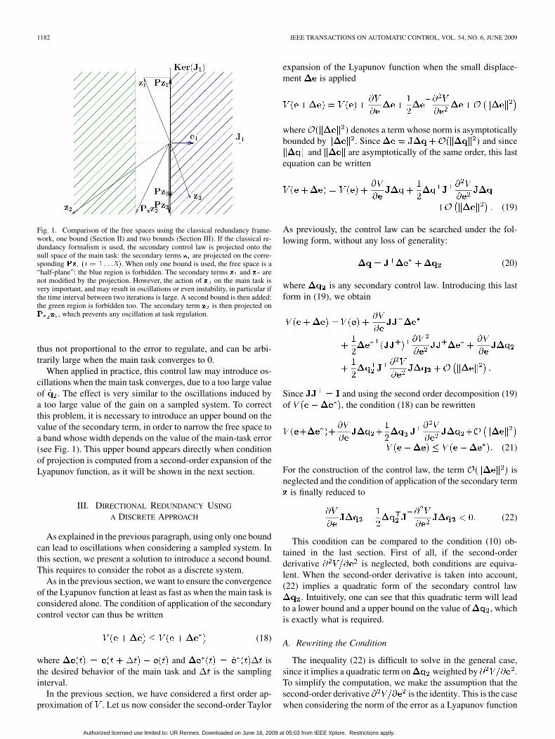
Fig. 1. Comparison of the free spaces using the classical redundancy frame-work, one bound (Section II) and two bounds (Section III). If the classical re-dundancy formalism is used, the secondary control law is projected onto thenull space of the main task: the secondary terms � are projected on the corre-sponding �� . When only one bound is used, the free space is a“half-plane”: the blue region is forbidden. The secondary terms � and � arenot modified by the projection. However, the action of � on the main task isvery important, and may result in oscillations or even instability, in particular ifthe time interval between two iterations is large. A second bound is then added:the green region is forbidden too. The secondary term � is then projected on� � , which prevents any oscillation at task regulation.

thus not proportional to the error to regulate, and can be arbi-trarily large when the main task converges to 0.

When applied in practice, this control law may introduce os-cillations when the main task converges, due to a too large valueof . The effect is very similar to the oscillations induced bya too large value of the gain on a sampled system. To correctthis problem, it is necessary to introduce an upper bound on thevalue of the secondary term, in order to narrow the free space toa band whose width depends on the value of the main-task error(see Fig. 1). This upper bound appears directly when conditionof projection is computed from a second-order expansion of theLyapunov function, as it will be shown in the next section.

III. DIRECTIONAL REDUNDANCY USING

A DISCRETE APPROACH

As explained in the previous paragraph, using only one boundcan lead to oscillations when considering a sampled system. Inthis section, we present a solution to introduce a second bound.This requires to consider the robot as a discrete system.

As in the previous section, we want to ensure the convergenceof the Lyapunov function at least as fast as when the main task isconsidered alone. The condition of application of the secondarycontrol vector can thus be written

(18)

where and isthe desired behavior of the main task and is the samplinginterval.

In the previous section, we have considered a first order ap-proximation of . Let us now consider the second-order Taylor

expansion of the Lyapunov function when the small displace-ment is applied

where denotes a term whose norm is asymptoticallybounded by . Since and since

and are asymptotically of the same order, this lastequation can be written

(19)

As previously, the control law can be searched under the fol-lowing form, without any loss of generality:

(20)

where is any secondary control law. Introducing this lastform in (19), we obtain

Since and using the second order decomposition (19)of , the condition (18) can be rewritten

(21)

For the construction of the control law, the term isneglected and the condition of application of the secondary term

is finally reduced to

(22)

This condition can be compared to the condition (10) ob-tained in the last section. First of all, if the second-orderderivative is neglected, both conditions are equiva-lent. When the second-order derivative is taken into account,(22) implies a quadratic form of the secondary control law

. Intuitively, one can see that this quadratic term will leadto a lower bound and a upper bound on the value of , whichis exactly what is required.

A. Rewriting the Condition

The inequality (22) is difficult to solve in the general case,since it implies a quadratic term on weighted by .To simplify the computation, we make the assumption that thesecond-order derivative is the identity. This is the casewhen considering the norm of the error as a Lyapunov function



Fig. 2. Two sets � (the circle) and� (the dashed rectangle) in dimension 2.The canonical basis of the task space is �� . The SVD coordinate frame is�� . In this basis, the set � is simply a ball of euclidean norm ��, withcenter �� and radius ��, and the set � is the same parameters ball of norm�� . The four points � , � , � and � are projected into � as a matter ofexample. Their projection is respectively�� ,�� ,�� and�. The projectionis realized by applying the projection operator computed in Section III-C.

, which is a very classical solution. We thusconsider the following condition:

(23)

where .As in the previous section, the SVD bases are introduced to

reduce the complexity to the case where the Jacobian is diag-onal. We note and . Condition (23) can besimply written as

(24)

By adding the term to both sides of the in-equality, the following factorization is obtained:

(25)

B. Construction of the Free Space

For some vector , let be the set

(26)

is the ball of radius and center . It is representedon Fig. 2 in the case of a 2-D vector space. Using this definition,the set of all the possible secondary motions such thatrespects the condition (23) is characterized easily. This condi-tion can thus be written as

(27)

Given an arbitrary secondary command , we now want tomodify this vector to obtain a second term that respectsthis condition. If belongs to the free space , it can be

directly added to the primary control law . Other-wise, it has to be projected into the free space. The projectionoperator is computed using the analytical parametrization of

. By developing the square of the norms in (25), it iseasy to obtain after some simple calculations

(28)

This last condition imposes a decrease of the norm of the error.As in the previous section, we reduce the condition by imposingthe decrease of each component of the error. The set isreduced to its Cartesian subset. A sufficient condition is thus

(29)

The set defined by (29) is noted . It is represented with

the corresponding set on Fig. 2. is in fact theball defined by the norm , where

(30)

C. Construction of the Projection Operator

The projection operator into the free space is noted. It is a vectorial operator that transforms any vector into a

secondary control law such that (29) is respected,and such that the distance is minimal. Using the an-alytical characterization of the free space given by (29), thisprojection operator can be computed component by componentwithin basis .

Since , (29) can be developed by dividing by(if is not zero): belongs to the free space of the maintask if and only if

(31)

For each component of , the closest that respects (31)can be computed. By analyzing each case separately, the generalexpression of is deduced

if or

if

if

if andif and

otherwise.(32)

This equation can be written under a matricial form

. . . (33)



Fig. 3. Comparison of the projection operators obtained with the classical redundancy formalism, and with the directional redundancy, first order (15) and secondorder (33).

where

if or

if

if

if andif and

otherwise.

As in Section II, the operator is not linear: the term isthus not linear in . Moreover, in that case, the matrix is nota projection matrix (its diagonal should be composed only of 0and 1). It is only the matricial form of the non linear projectionoperator .

D. Control Law

The projection operator is computed into the SVD basesand . We note this operator into the canonical basis of

the joint space

(34)

The control law is finally written. Thanks to the matricial form, the obtained form is very close to the classical redundancy

form given in (4)

(35)

where is an arbitrary vector, used to perform a secondary taskwithout disturbing the decreasing speed of the main task error.

E. Comparisons and Conclusion

A comparison between the two projection operators built inSections II and III with the classical projection operator is givenin Fig. 3. As in the classical formalism, the projection operator isused to transform any secondary vector into a secondary controllaw that does not disturb the main task. Within the same basis

, the projection operator of the classical redundancy is also adiagonal matrix, but whose coefficients are

ifotherwise.

(36)

In other terms, the first projection operator (15) that we have de-fined has more non zero coefficients. When a component of themain task function is not zero, a DOF is freed up. Furthermore,the proposed formalism accelerates the decreasing of each com-ponent of the error and takes the secondary task into account inthe same way.

Compared to the projection operator (15), the operator (33)induces an alleviation if the secondary control law is too impor-tant wrt. the error value. In particular, at task completion, whenthe error vector is nearly zero, this allows to reduce the effect ofthe secondary term, and to avoid any oscillation.

IV. STABILITY OF THE CONTROL LAW

The definition of the control law (35) and the associate pro-jector lead to the following theorem:

Theorem 4.1: Let be any task function whose Jacobianis full rank. If the following control law:

(37)

is applied to the robotic system, where:• is a stable vector field such that

respects .• is any secondary control law, and is defined by (33).

then, given that is sufficiently small, the error asymptoti-cally converges to zero.

Proof: From (21), it is possible to write

(38)

By construction of , we know that respects (22).Introducing (22) in the previous equation, we obtain

(39)

Subtracting from both side of the inequality finally gives

(40)

where and. It is thus possible to find small enough to have. Since has the same order as and given that

is sufficiently small, then . By definition of ,is negative, which proves that is a correct Lyapunov

function for control law (37).Remark 1: We have not been able to determine any theoret-

ical value of to ensure the stability for any large value of. In practice, the value of used to compute the control law

could be chosen smaller than the actual value of the samplinginterval of the control input. This choice allows ensuring thepractical stability of the system when is large. However, wehave not used the possibility to tune this parameter in the ex-periments presented in the following: has been chosen equal



to the system time interval. No unstability have been noticedduring the experimental setup.

Remark 2: Theorem 4.1 supposes that the desired evolutionis such that is negative. When as

classically done, this last hypothesis is simply obtained bychoosing the gain and the step size small enough.

Theorem 4.1 only gives the asymptotic convergence of themain task. It does not say anything about the secondary task.Since the main task has priority, the convergence of the sec-ondary task can not be ensured in the general case. However,it is expected to obtain at least the convergence of the part of thesecondary task located inside the null space of the main task,that is to say

(41)

In the general case where the secondary task can be any -di-mensional vector, nothing can be proved. We thus limit the sta-bility study to the classical case where the secondary task is thegradient of a cost function to be minimized [13], [17]. Indeed,the secondary tasks used to experiment the control law on therobot are derived from a cost function (see Section V-B). UsingTheorem 4.1, it is easy to deduce the asymptotic convergence toa region where the secondary task gradient is in the null space ofthe main task, that is to say the cost function is asymptoticallyminimized under the constraint .

Corollary 4.1: Let be any positive convex function de-fined on the joint space. Using the hypotheses of Theorem 4.1,if the control law (37) is applied to the robotic system, with

, then the cost function is asymptotically mini-mized under the constraint .

Proof: The control law is asymptotically equivalent to(from Theorem 4.1)

(42)

We assume that does not depend of the independent time vari-able

(43)

By introducing (42) in (43), we obtain

(44)

Since is definite non-negative for any vector (due to theform (33) of the coefficients of the equivalent diagonal matrix

), we finally obtain

(45)

This result is sufficient to prove the stability of the secondarycriterion, but does not prove that the second criterion is globallyasymptotically minimized ( should be negative, and it is onlynon-positive). However, it proves that is stable and decreasesuntil becomes null, that is the minimum under theconstraint is reached.

A similar Lyapunov function can be given for the controlscheme using the classical redundancy formalism. Let bethe secondary cost function value over time using the classicalredundancy formalism scheme, and let be the secondary

cost function value using the scheme proposed in Theorem 4.1.Through the misuse of notation , we can write

(46)

(47)

Since the singular values of are all greater than or equalto the singular values of (due to (33) and (36)), the followinginequality can be written:

(48)

The cost function converges to similar local minima using bothschemes. However, this last inequality proves that the conver-gence is faster using the directional redundancy.

To conclude, we have shown in this section that the globalminimization of is of course not necessarily ensured. Thesystem converges to a local minimum imposed by the constraint

as expected. However Theorem 4.1 and Corollary 4.1prove that the system is globally stable, and asymptotically con-verges to the main task completion and to the best reachablelocal minimum of the secondary task.

V. APPLICATION TO VISUAL SERVOING

All the work presented above has been realized under the onlyhypothesis that the main task is a task function as describedin [21]. The method is thus fully general and can be appliedfor numerous sensor-based closed-loop control problems. Forthis article, the method has been applied to visual servoing. Inthe experiments described in the next section, the robot has tomove with respect to a visual target, and simultaneously to takeinto account a secondary control law. For the simulations, thissecondary term was simply an arbitrary velocity. For the exper-iments on the real robot, the joint limits and possible occlusionswere considered. In this section, the classical visual servoingformalism is first quickly recalled (Section V-A). Two avoid-ance laws are then presented for joint-limit and visual-occlu-sion avoidance, based on the gradient of a cost function [13],[15], [17]. We have chosen to use a solution proposed from pathplanning [18] which ensures an optimal computation of the gra-dient by the use of a pseudo inverse. This general method ispresented in Section V-B and the two cost functions are givenin Section V-C.

A. Main Task Function Using Visual Servoing

In the experiments presented below, an eye-in-hand robot hasto move with respect to a visual target (a sphere in simulationand a rectangle composed of four points easily detectable for theexperiments on a real robot). By choosing a very simple target,the experiments have focused on the control part of the work.

The task function used in the following is defined as thedifference between the visual features computed at the currenttime and the visual features extracted from the desired image[7], [12]:

(49)

The interaction matrix related to is defined such that, where is the camera instantaneous velocity. From (49),



it is clear that the interaction matrix and the task Jacobianare linked by the relation

(50)

where the matrix denotes the robot Jacobian andis the matrix that relates the camera instantaneous velocity

to the variation of the chosen camera pose parametrization. The classical proportional control law

was used. The control law finally used in the experiment is then

(51)

where can be any vector used to realize a secondary task.In the experiments presented below, the target projection in

the image is a continuous region (an ellipse in simulation,a quadrilateral on the real robot). In order to have a better andeasier control over the robot trajectory, six approximatively de-coupled visual features are chosen as proposed in [23].

The two first features are the position and of the centerof gravity, controlling the target centering. The third featurecontrols the distance between the camera and the target. It isbased on the area of the object in the image. The fourth feature

is defined as the orientation of the object in the image and ismainly linked to the rotational motion around the optical axis.The two last features and are defined from third ordermoments to decouple the translational velocities and fromtheir corresponding rotational velocities and . The readeris invited to refer to [23] for more details and for the analyticalform of the interaction matrix of the chosen visual features.

For the experiments on the real robot, the observed region isthe image of a rectangle. The six features can thus be used tocontrol the six DOF of the robot. For the second experiment onthe robot however, only the four first features are used, to in-troduce some redundancy in the control system. For the experi-ments in simulation, the ellipse region is the image of a sphere.Only the three first feature can be used, and control three DOFof the robot.

B. Cost Function for Avoidance

The secondary task can be used to minimize the constraintsimposed by the environment. The constraints are described bya cost function. The gradient of this cost function can beconsidered as an artificial force, pushing the robot away fromthe undesirable configurations.

The cost function is expressed directly in the space of theconfiguration to avoid (e.g. the cost function of visual-occlu-sion constraint is expressed in the image space). Let be aparametrization of this space. The cost function can be written

. The optimal corresponding artificial force isproved to be [18]

(52)

Note the use of the Jacobian pseudo inverse in the final artificialforce formulation. Classical methods propose generally to usesimply the transpose of the Jacobian, the artificial force beingthen . Since the pseudo inverse

provides the least-square solution, the resulting artificial force(52) is the most efficient one at equivalent norm.

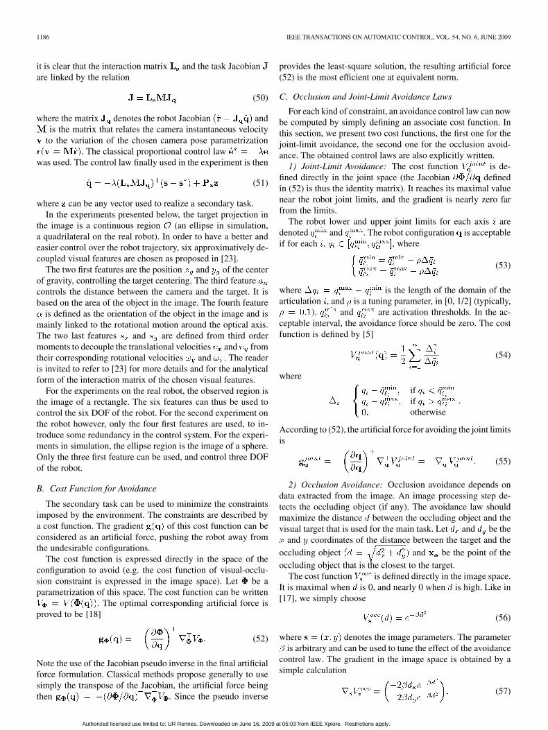
C. Occlusion and Joint-Limit Avoidance Laws

For each kind of constraint, an avoidance control law can nowbe computed by simply defining an associate cost function. Inthis section, we present two cost functions, the first one for thejoint-limit avoidance, the second one for the occlusion avoid-ance. The obtained control laws are also explicitly written.

1) Joint-Limit Avoidance: The cost function is de-fined directly in the joint space (the Jacobian definedin (52) is thus the identity matrix). It reaches its maximal valuenear the robot joint limits, and the gradient is nearly zero farfrom the limits.

The robot lower and upper joint limits for each axis aredenoted and . The robot configuration is acceptableif for each , , where

(53)

where is the length of the domain of thearticulation , and is a tuning parameter, in [0, 1/2] (typically,

). and are activation thresholds. In the ac-ceptable interval, the avoidance force should be zero. The costfunction is defined by [5]

(54)

where

ififotherwise

According to (52), the artificial force for avoiding the joint limitsis

(55)

2) Occlusion Avoidance: Occlusion avoidance depends ondata extracted from the image. An image processing step de-tects the occluding object (if any). The avoidance law shouldmaximize the distance between the occluding object and thevisual target that is used for the main task. Let and be the

and coordinates of the distance between the target and theoccluding object and be the point of theoccluding object that is the closest to the target.

The cost function is defined directly in the image space.It is maximal when is 0, and nearly 0 when is high. Like in[17], we simply choose

(56)

where denotes the image parameters. The parameteris arbitrary and can be used to tune the effect of the avoidance

control law. The gradient in the image space is obtained by asimple calculation

(57)



Fig. 4. Experiment A: main task error and projection operator rank using theclassical redundancy formalism. The projection operator rank is always 3. Themain task error is not modified by the secondary task: it is a perfect exponentialdecrease.

The artificial force that avoids the occlusions can be now com-puted using (52). The transformation from the image space tothe joint space is given by

(58)

where and are the transformation matrices defined in (50),and is the well-known interaction matrix related to the imagepoint [12].

VI. EXPERIMENTAL RESULTS

Three different experiments have been realized to highlightthe advantages of our method. The first one has been realizedin simulation to study in detail the differences between classicalredundancy and directional redundancy. The two others experi-ments have been realized with a real robot, the first one with allDOF constrained by the main task (redundancy is available onlythrough the directional redundancy framework), the second onewith four of the six robot DOF constrained by the main task.

A. Experiments in Simulation

The first experiments have been realized in simulation. It wasthus possible to control all the parameters of the experiment tostudy the control law in depth. In particular, the sensor noisewas easy to tune. In this experiment, the robot has to positionwith respect to a sphere. The main task is composed of threefeatures: center of gravity and sphere area in theimage. Three DOF remain free using the classical redundancyformalism. The secondary task is simply a displacement alongthe X-axis of the camera

(59)

The first part of the experiment was realized without anynoise in the measures. A summary is provided in Figs. 4–7. Thesecond part studies the effects of the sensor noise on the control

Fig. 5. Experiment A: main task error and projection operator rank using thedirectional redundancy formalism. The rank of the projection operator is notconstant during the servo. At the beginning of the servo, the DOF correspondingto Components � and � are available for the secondary task. The projectionoperator rank is thus 5. The DOF corresponding to � is used by the secondarytask. The decrease is thus faster than required by the main task. When � be-comes null, the projection operator rank decreases (Iteration 80). The DOF cor-responding to � is available until Iteration 300. At this instant, the main taskerror is null. No additional DOF remains free. The projection operator is thusthe same than the one obtained by the classical formalism.

Fig. 6. Experiment A: comparison of the projected secondary task using theclassical and the directional redundancy formalism. While the first componentof the main task is not null (until Iteration 80), two components of the secondarytasks are taken into account using the directional redundancy formalism, butnullified by the classical formalism. (a) Classical redundancy formalism; (b)directional redundancy formalism.

law, and proposes a simple hysteresis comparator to filter thenoise when computing the projection operator.

1) Comparison With the Classical Redundancy Formalism:Using the classical redundancy formalism, the projection-oper-ator rank is 3 during the whole execution (see Fig. 4). The errorbehavior is a perfect exponential decrease, as specified by .



Fig. 7. Experiment A: control law using the directional redundancy formalism.The norm of the translational and rotational velocities are represented. The ve-locity changes at Iteration 80, corresponding to the projection-operator rank de-crease (see Fig. 5).

On the contrary, when using the formalism proposed above, theprojection-operator rank is greater than 3 while the error of themain task is not null. As can be seen on Fig. 5, the convergenceof the first component of the main-task error is accelerated bythe secondary task. When it reaches 0, the projection operatorlooses a rank. The third component of the error does not cor-respond to any part of the secondary task, and is thus let un-touched. The corresponding DOF is available but not used bythe secondary task. When reaches 0, the projection operatorlooses another rank. From this point, there is no difference atall between the two redundancy formalisms: the two projectionoperators are equal, and the robot behavior is the same.

The effect of the projection operator on the secondary task isshown in Fig. 6. While Component is not null, a part of thesecondary task is nullified by the classical projection operator,but taken into account by the proposed control law. Intuitively,the main task is composed of two parts: centering and zooming.Since the secondary task is a translation along X-axis, it modi-fies the centering. When the main task is realized, the projectionoperator mainly generates an artificial rotation to compen-sate the secondary velocity and thus preserves the centering.In the initial configuration presented here, the secondary taskhas an acceptable influence on the centering, since it helps torealize the centering. It is thus accepted when using the direc-tional redundancy formalism while the object is not centered inthe image. As soon as the centering is realized, the part of thesecondary task that modifies the centering is rejected, and nul-lified by the projection operator. Component which is partof the centering converges thus faster than using the classicalredundancy formalism. The DOF corresponding to the zoom isalso available using the directional redundancy. However, sincethe secondary task has no effect on the zoom, it is not used andComponent of the main task which corresponds to the zoomconverges like when using the classical formalism.

2) In Presence of Noise: A white noise is added directlyto the computation of the main-task error. The error will thusnever reach . The task is considered to be completed when itis smaller than a threshold equals to the variance of the noise.The computation of the projection operator also requires to testif the components of the error is null: a DOF is available whenthe corresponding error component is not null but disappears

Fig. 8. Experiment A: main task error and projection operator rank using the di-rectional redundancy formalism in the presence of noise without any hysteresiscomparator. The projection operator rank increases each time an error compo-nent passes through the threshold.

Fig. 9. Experiment A: control law using the directional redundancy formalismin the presence of noise without any hysteresis comparator. A peak appears eachtime the projection operator rank increases.

as soon as the component reaches 0 (see (33)). Once again, theerror component is considered null if it is smaller than the noisevariance.

The main task error and the rank of the projection operatorare given in Fig. 8. As can be seen on this figure, the rank ofthe operator is very noisy. Since the rank is discrete, the whitenoise is amplified when computing the projection operator andinduces thus a very strong perturbation: each time the error in-creases above the threshold because of the noise, the projectionoperator rank increases. As can be seen on Fig. 9, the noise isamplified by the control law computation and a lot of strong dis-continuities appear in the control law.

3) Hysteresis Comparator: The problem is solved usinga simple principle known as the Schmitt trigger in electricalengineering [22]. Two thresholds are used to determine if theerror is null. The output of the comparison is not null if theerror is greater than the higher threshold; the output is null if theerror is smaller than the lower threshold. And when the erroris between the two thresholds, the output retains the previousvalue. The lower threshold is set to the noise variance, whichcorresponds to one standard deviation. The higher thresholdhas to be set so that an error greater than the threshold has avery low probability to be only due to noise. We have set itto three standard deviations of the noise, which correspond



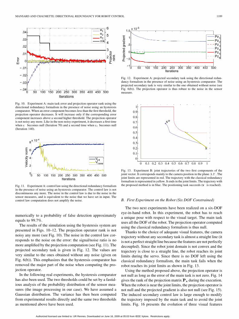
Fig. 10. Experiment A: main task error and projection operator rank using thedirectional redundancy formalism in the presence of noise using an hysteresiscomparator. When an error component becomes less than the first threshold, theprojection operator decreases. It will increase only if the corresponding errorcomponent increases above a second higher threshold. The projection operatoris not noisy any more. Like in the non-noisy experiment, it decreases a first timewhen � becomes null (Iteration 70) and a second time when � becomes null(Iteration 140).

Fig. 11. Experiment A: control law using the directional redundancy formalismin the presence of noise using an hysteresis comparator. The control law is notdiscontinuous any more. The noise in the control law is due to the noise in thesensor measures, and is equivalent to the noise that we have set in input. Thecontrol law computation does not amplify the noise.

numerically to a probability of false detection approximatelyequals to 99.7%.

The results of the simulation using the hysteresis system arepresented in Figs. 10–12. The projection operator rank is notnoisy any more (see Fig. 10). The noise in the control law cor-responds to the noise on the error: the signal/noise ratio is nomore amplified by the projection computation (see Fig. 11). Theprojected secondary task is given in Fig. 12. The values arevery similar to the ones obtained without any noise (given onFig. 6(b)). This emphasizes that the hysteresis comparator hasremoved the major part of the noise when computing the pro-jection operator.

In the following real experiments, the hysteresis comparatorhas also been used. The two thresholds could be set by a fastid-ious analysis of the probability distribution of the sensor mea-sures (the image processing in our case). We have assumed aGaussian distribution. The variance has then been computedfrom experimental results directly and the same two thresholdsas mentioned above have been used.

Fig. 12. Experiment A: projected secondary task using the directional redun-dancy formalism in the presence of noise using an hysteresis comparator. Theprojected secondary task is very similar to the one obtained without noise (seeFig. 6(b)). The projection operator is thus robust to the noise in the sensormeasure.

Fig. 13. Experiment B: joint trajectories of the two first components of thejoint vector. It corresponds mainly to the camera position in the plane�� . Thejoint limits are represented in red. The trajectory with the classical redundancyformalism is represented in yellow. It ends in the joint limits. The trajectory withthe proposed method is in blue. The positioning task succeeds (� is reached).

B. First Experiment on the Robot (Six DOF Constrained)

The two next experiments have been realized on a six-DOFeye-in-hand robot. In this experiment, the robot has to reacha unique pose with respect to the visual target. The main taskuses all the DOF of the robot. The projection operator computedusing the classical redundancy formalism is thus null.

Thanks to the choice of adequate visual features, the cameratrajectory without any secondary task is almost a straight line (itis not a perfect straight line because the features are not perfectlydecoupled). Since the robot joint domain is not convex and thetrajectory is close to a straight line, the robot reaches its jointlimits during the servo. Since there is no DOF left using theclassical redundancy formalism, the main task fails when therobot reaches its joint limits as shown in Fig. 13.

Using the method proposed above, the projection operator isnot null as long as the error of the main task is not zero. Fig. 14gives the rank of the projection matrix during the execution.When the robot is near the joint limits, the projection operator isnot null and the projected gradient is also not null (see Fig. 15).The induced secondary control law is large enough to modifythe trajectory imposed by the main task and to avoid the jointlimits. Fig. 16 presents the evolution of three visual features



Fig. 14. Experiment B: rank of the projection operator computed using theproposed approach during the servo.

Fig. 15. Experiment B: projected gradient using the proposed method. The sec-ondary control law mainly increases the third component of the joint speed, thatcorresponds to the speed along the optical axis.

Fig. 16. Experiment B: evolution of the visual features when applying the pro-posed method. The two features � and � (plotted in red and blue) are modi-fied by the avoidance law. On the opposite, feature � (plotted in green) is notmodified.

whose value is modified by the secondary control law. The pro-jection operator mainly accelerates the decreasing speed of fea-tures and controlling the centering (pan) and the motionalong the optical axis. Using the framework presented above,it is thus possible to free up some additional DOF that are notavailable within the classical redundancy formalism. The maintask is correctly completed, and the servo is not slowed by thesecondary control law.

C. Second Experiment on the Robot (Four DOF Constrained)

In the previous experiment, no avoidance law could be takeninto account by the classical redundancy formalism. It was thus

Fig. 17. Experiment C: main phases of the servo (a) without avoidance,(b) with the avoidance law projected using the classical redundancy formalism,and (c) using the directional redundancy. The pictures are taken by theembedded camera. The visual target is the four-white-points rectangle. Theoccluding object is the orange shape that appears in the left of the image.

Fig. 18. Experiment C: norms of the projected gradient using the classical re-dundancy formalism (yellow) and of the projected gradient using the proposedapproach (blue). The projected gradient using the classical framework is lowerthan the one obtained with our method.

easy to see that the performance of our framework is better. Thenext experiment will point out that, even when DOF are avail-able for avoidance, a better behavior of the system is obtainedby considering a larger free space as done above.

The main task is composed of four visual features. The robothas to move in order to center the object in the image, to rotateit properly around the optical axis, and to bring the camera at adistance of 1.5 m of the target using . TwoDOF are thus available, that correspond mainly to motions ona sphere whose center is the target. During the servo, an objectmoves between the camera and the visual target, leading to anocclusion. The two available DOF are used to avoid this occlu-sion, as explained in Section V-C-2.

Without any avoidance law, the visual target is quickly oc-cluded, which makes the servo to fail [Fig. 17(a)]. Using theclassical redundancy formalism, the gradient is projected into atwo-dimensional space. Its norm is thus reduced, and the sec-ondary control law is not fast enough to avoid the occlusion.Mainly, the projection operator forbids the motion along theoptical axis, which is controlled by one of the features of themain task (Fig. 18). This motion is available using our approach(Fig. 19). The robot velocity is thus fast enough to avoid the oc-clusion [Fig. 17(c)]. The decreasing speed of some visual fea-tures has been accelerated to enlarge the free space of the firsttask (Fig. 20). When the occlusion ends, the features decreaseis no longer modified. The trajectory of the camera is given inFig. 21. When the occlusion is not taken into account, the tra-jectory is a straight line. When taking the occlusion into accountusing the classical redundancy formalism, the additional motion



Fig. 19. Experiment C: translational velocities of the avoidance control lawprojected using the classical redundancy formalism (a) and projected using theproposed approach (b). The motions along the camera axis (red) are not nullusing the proposed control law.

Fig. 20. Experiment C: decreasing error of the visual features. The occlusionavoidance begins at Event 1. The decrease of the feature plotted in red is accel-erated. The occlusion is completely avoided after Event 2. The decrease goesback to a normal behavior.

Fig. 21. Experiment C: comparison of the trajectory of the robot in the planeperpendicular to the target.

induces a translation that modifies the trajectory. When the di-rectional redundancy is used, the robot mainly accelerates thetranslation toward the camera.

VII. CONCLUSION

In this paper, we have proposed a new general method to inte-grate a secondary term to a first task having priority. Our frame-work is based on a generalization of the classical redundancy for-malism. We have shown that it is possible to enlarge the numberof the available DOF, and thus to improve the performance of theavoidance control law. This control scheme has been validated insimulation and on a six-DOF eye-in-hand robotic platform wherethe robot had to reach a specific pose with respect to a visualtarget, and to avoid joint limits and occlusions.

We have shown that it is possible to find DOF during theaccomplishment of a full-constraining task, and to enhance theavoidance process even when enough DOF are available.

Our current works aim at realizing a reactive servo, able toperform a full constraining task and to simultaneously take intoaccount the perturbations due to a real robotic system. The gen-eral idea is to free up as many DOF as possible to perform theavoidance of any obstacle encountered during the servo [16].Using the method proposed in this article, additional DOF arecollected at the very bottom level, directly in the control law. Anavoidance can be realized even when the adequate DOF are al-ready used by the main task. However, the number of DOF canbe insufficient for example when the obstacles are numerous.We now focus on the choice of the main task, to obtain addi-tional DOF by modifying the main task from a higher level.

ACKNOWLEDGMENT

The authors would like to thank the anonymous reviewers fortheir valuable comments which allow great improvements in theclarity and presentation of the paper.

REFERENCES

[1] P. Baerlocher and R. Boulic, “An inverse kinematic architecture en-forcing an arbitrary number of strict priority levels,” Visual Comput.,vol. 6, no. 20, pp. 402–417, Aug. 2004.

[2] A. Ben-Israel and T. Greville, Generalized Inverses: Theory and Ap-plications. New York: Wiley-Interscience, 1974.

[3] T. Chang and R. Dubey, “A weighted least-norm solution basedscheme for avoiding joints limits for redundant manipulators,” IEEETrans. Robot. Automat., vol. 11, no. 2, pp. 286–292, Apr. 1995.

[4] F. Chaumette and S. Hutchinson, “Visual servo control, part i: Basicapproaches,” IEEE Robot. Automat. Mag., vol. 13, no. 4, pp. 82–90,Dec. 2006.

[5] F. Chaumette and E. Marchand, “A redundancy-based iterative schemefor avoiding joint limits: Application to visual servoing,” IEEE Trans.Robot. Automat., vol. 17, no. 5, pp. 719–730, Oct. 2001.

[6] N. Cowan, J. Weingarten, and D. Koditschek, “Visual servoing via nav-igation functions,” IEEE Trans. Robot. Automat., vol. 18, no. 4, pp.521–533, Aug. 2002.

[7] B. Espiau, F. Chaumette, and P. Rives, “A new approach to visualservoing in robotics,” IEEE Trans. Robot. Automat., vol. 8, no. 3, pp.313–326, Jun. 1992.

[8] J. Feddema and O. Mitchell, “Vision-guided servoing with feature-based trajectory generation,” IEEE Trans. Robot. Automat., vol. 5, no.5, pp. 691–700, Oct. 1989.

[9] G. Hager, “Human-machine cooperative manipulation with vi-sion-based motion constraints,” in Proc. Workshop Visual Servoing,IEEE/RSJ Int. Conf. Intell. Robot. Syst. (IROS’02), Lausane, Switzer-land, Oct. 2002, [CD ROM].

[10] H. Hanafusa, T. Yoshikawa, and Y. Nakamura, “Analysis and control ofarticulated robot with redundancy,” in Proc. IFAC, 8th Triennal WorldCongress, Kyoto, Japan, 1981, vol. 4, pp. 1927–1932.

[11] Visual Servoing: Real Time Control of Robot Manipulators Based onVisual Sensory Feedback, K. Hashimoto, Ed. Singapore: World Sci-entific, 1993, vol. 7.

[12] S. Hutchinson, G. Hager, and P. Corke, “A tutorial on visual servocontrol,” IEEE Trans. Robot. Automat., vol. 12, no. 5, pp. 651–670,Oct. 1996.

[13] O. Khatib, “Real-time obstacle avoidance for manipulators and mobilerobots,” Int. J. Robot. Res., vol. 5, no. 1, pp. 90–98, Spring, 1986.

[14] C. Klein and S. Kittivatcharapong, “Optimal force distribution for thelegs of a walking machine with friction cone constraints,” IEEE Trans.Robot. Automat., vol. 6, no. 1, pp. 73–85, Feb. 1990.

[15] A. Liégeois, “Automatic supervisory control of the configuration andbehavior of multibody mechanisms,” IEEE Trans. Syst., Man Cybern.,vol. 7, no. 12, pp. 868–871, Dec. 1977.

[16] N. Mansard and F. Chaumette, “Task sequencing for sensor-based con-trol,” IEEE Trans. Robotics, vol. 23, no. 1, pp. 60–72, Feb. 2007.

[17] E. Marchand and G. Hager, “Dynamic sensor planning in visual ser-voing,” in Proc. IEEE/RSJ Int. Conf. Intell. Robot. Syst. (IROS’98),Leuven, Belgium, May 1998, pp. 1988–1993.



[18] Y. Mezouar and F. Chaumette, “Path planning for robust image-basedcontrol,” IEEE Trans. Robot. Automat., vol. 18, no. 4, pp. 534–549,Aug. 2002.

[19] B. Nelson and P. Khosla, “Strategies for increasing the tracking regionof an eye-in-hand system by singularity and joint limits avoidance,” Int.J. Robot. Res., vol. 14, no. 3, pp. 255–269, Jun. 1995.

[20] J. Rosen, “The gradient projection method for nonlinear program-mimg, part i, linear constraints,” SIAM J. Appl. Math., vol. 8, no. 1,pp. 181–217, Mar. 1960.

[21] C. Samson, M. Le Borgne, and B. Espiau, Robot Control: The TaskFunction Approach. Oxford, U.K.: Clarendon Press, 1991.

[22] O. Schmitt, “A thermionic trigger,” J. Scientific Instrum., vol. 15, pp.24–26, 1938.

[23] O. Tahri and F. Chaumette, “Point-based and region-based image mo-ments for visual servoing of planar objects,” IEEE Trans. Robotics, vol.21, no. 6, pp. 1116–1127, Dec. 2005.

Nicolas Mansard graduated from École NationaleSupérieure d’Informatique et de MathématiquesAppliquées, Grenoble, France and received the M.S.(DEA) degree in robotics and image processing fromthe University Joseph Fourier, Grenoble, in 2003and the Ph.D. degree in computer science from theUniversity of Rennes, Rennes, France, in 2006.

He spent three years in the Lagadic research group,IRISA, INRIA-Bretagne. He then spent one year atStanford University, Stanford, CA, and one year withJRL-Japan, AIST, Tsukuba, Japan. He is currently

with LAAS/CNRS, Toulouse, France, in the GEPETTO group. His researchinterests are concerned with sensor-based robot animation, and more specifi-cally the integration of reactive control schemes into real robot and humanoidapplications.

Dr. Mansard received the Best Thesis Award from the French Research GroupGdR-MACS, in 2006, the Best Thesis Award from the Society for Telecomu-nication and Computer Science (ASTI), in 2007, and the Best Thesis Award ofthe Région Bretagne.

François Chaumette (M’98) received the M.S. de-gree from École Nationale Supérieure de Mécanique,Nantes, France, in 1987 and the Ph.D. degree in com-puter science from the University of Rennes, Rennes,France, in 1990.

Since 1990, he has been with IRISA/INRIARennes Bretagne Atlantique, where he is “Directeurde recherche” and Head of the Lagadic Group. Heis the coauthor of more than 50 papers publishedin international journals on the topics of roboticsand computer vision. His research interests include

robotics and computer vision, especially visual servoing and active perception.Dr. Chaumette received several awards including the AFCET/CNRS Prize

for the Best French Thesis on Automatic Control in 1991 and the King-Sun FuMemorial Best IEEE TRANSACTIONS ON ROBOTICS AND AUTOMATION PaperAward in 2002. He has been the Associate Editor of the IEEE TRANSACTIONS

ON ROBOTICS from 2001 to 2005 and is now in the Editorial Board of the Inter-national Journal of Robotics Research. He has served over the last five years onthe program committees for the main conferences related to robotics and com-puter vision.


directional redundancy for robot control · automatic control, institute of electrical and...

Documents