diplomarbeit - cryptology eprint archive · diplomarbeit algebraic attacks specialized for f 2...
TRANSCRIPT

Diplomarbeit
Algebraic attacks specialized for F2
Thomas Dullien
28. August 2008
Betreuer: Roberto Avanzi
HGI, University of Bochum

The picture on the title shows the number of monomials that occur inintermediate results of the pseudo-euclidian algorithm on random quadraticequation systems in 14 variables.

Contents
Introduction 5
1 Definitions and Notation 91.1 Essentials . . . . . . . . . . . . . . . . . . . . . . . . . . . . . 91.2 Representation of Boolean Functions . . . . . . . . . . . . . . 13
1.2.1 Algebraic Normal Form (ANF) . . . . . . . . . . . . . 131.2.2 Hadamard-Transform . . . . . . . . . . . . . . . . . . 171.2.3 Walsh-Transform . . . . . . . . . . . . . . . . . . . . . 18
1.3 The ring of Boolean functions as a lattice . . . . . . . . . . . 181.4 The MQ problem . . . . . . . . . . . . . . . . . . . . . . . . . 18
2 Generating Equations 202.1 Generating Equations for LFSR-based stream ciphers . . . . 20
2.1.1 Generating equations for simple combiners . . . . . . 222.1.2 Generating equations for combiners with memory . . . 222.1.3 Z-functions . . . . . . . . . . . . . . . . . . . . . . . . 23
2.2 Generating Equations for block ciphers . . . . . . . . . . . . . 232.2.1 Algebraic description of an SPN . . . . . . . . . . . . 232.2.2 Naive attempts at generating equations . . . . . . . . 242.2.3 Generating equations for PRESENT . . . . . . . . . . 252.2.4 Weakening to 40 bits . . . . . . . . . . . . . . . . . . . 282.2.5 The question of intermediate variables . . . . . . . . . 292.2.6 The geometry of introducing variables . . . . . . . . . 29
2.3 Summary . . . . . . . . . . . . . . . . . . . . . . . . . . . . . 30
3 Grobner basis and the Buchberger Algorithm 343.1 Introduction . . . . . . . . . . . . . . . . . . . . . . . . . . . . 34
3.1.1 Term Orders . . . . . . . . . . . . . . . . . . . . . . . 353.1.2 Macaulay’s Basis Theorem . . . . . . . . . . . . . . . 353.1.3 Multivariate Division . . . . . . . . . . . . . . . . . . . 363.1.4 S-Polynomials . . . . . . . . . . . . . . . . . . . . . . . 37
3.2 The classical Buchberger Algorithm . . . . . . . . . . . . . . 373.2.1 Interpretation: An almost purely syntactic algorithm . 37
3

4
3.3 Maximum sizes of polynomials in the computation . . . . . . 39
4 The Raddum-Semaev-Algorithm 404.1 The original description . . . . . . . . . . . . . . . . . . . . . 404.2 A geometric view . . . . . . . . . . . . . . . . . . . . . . . . . 424.3 An algebraic-geometric view . . . . . . . . . . . . . . . . . . . 434.4 Raddum-Semaev Algorithm . . . . . . . . . . . . . . . . . . . 44
4.4.1 Algebraization . . . . . . . . . . . . . . . . . . . . . . 454.4.2 Summary . . . . . . . . . . . . . . . . . . . . . . . . . 46
5 Published Algebraic attacks 475.0.3 Lowering the degree by multiplication . . . . . . . . . 485.0.4 Lowering the degree by finding linear combinations . . 485.0.5 Faugere-Ars attack on nonlinear filters . . . . . . . . . 505.0.6 Experimental attack on Toyocrypt . . . . . . . . . . . 50
5.1 The notion of algebraic immunity . . . . . . . . . . . . . . . . 50
6 The Pseudo-Euclidian Algorithm 516.0.1 A naive first algorithm . . . . . . . . . . . . . . . . . . 51
6.1 Some empirical data . . . . . . . . . . . . . . . . . . . . . . . 536.1.1 Hard instances of MQ . . . . . . . . . . . . . . . . . . 536.1.2 Equation systems generated from cryptographic prob-
lems . . . . . . . . . . . . . . . . . . . . . . . . . . . . 556.2 Getting other information about the variety . . . . . . . . . . 55
6.2.1 Determining equality between variables . . . . . . . . 556.2.2 Monomial count and hamming weight . . . . . . . . . 576.2.3 Attempting solutions without calculating the product 57
6.3 Viewing the algorithm as traversal of a lattice . . . . . . . . . 576.4 The notion of approximation . . . . . . . . . . . . . . . . . . 60
6.4.1 Approximation of polynomials . . . . . . . . . . . . . 616.4.2 Re-visiting Courtois-Armknecht attacks on stream ci-
phers . . . . . . . . . . . . . . . . . . . . . . . . . . . 626.4.3 Constructing approximations . . . . . . . . . . . . . . 656.4.4 Constructing approximations: Complete failure . . . . 67
6.5 Conclusion (for now) . . . . . . . . . . . . . . . . . . . . . . . 67
7 Pseudo-Euclid over finite fields 697.1 Generalization to arbitrary finite fields . . . . . . . . . . . . . 69

Einleitung
Introduction
In his landmark paper, Shannon stated that breaking a good cipher should’require at least as much work as solving a system of simultaneous equationsin a large number of unknowns of a complex type’.
In the years since, most published cryptanalytic successes in symmet-ric cryptography were obtained by statistical or combinatorial weaknessesin the ciphers that were analyzed. Equation-system solving was not at theforefront, partially because most ciphers were built without a ’clean’ alge-braic structure in which to work, partially because efficient algorithms forthe algebraic solving of equation systems were not available.
Interest in algebraic methods for attacks on cryptosystems was revivedfrom two directions in the late 90’s and early 00’s: On the one side, cryp-tographers had attempted to build asymmetric systems from the hardnessof the MQ-problem (the problem of solving multivariate quadratic equationsystems over an arbitrary field). Patarin [Patarin95] showed how to break asignature scheme originally proposed by Matsumoto and Imai [MatImai88]as early as 1988 by making use of the special structure of the equationsin question. Several attempts at using general-purpose equation solvingalgorithms were made, resulting in the break of HFE [FauJou03] using anew Grobner-Base algorithm introduced the year before [Faugere02]. Thisshowed that more efficient algorithms for equation system solving could havea direct application in cryptanalysis.
The other direction from which interest in algebraic attacks was reignitedwas the emergence of Rijndael as the new advanced encryption standard(AES): Rijndael was designed to resist the standard statistical attacks andwas modeled to use only the ’normal’ field operations of F28 , yielding avery clean algebraic structure. Soon, several researchers proposed methodsthat allowed modeling Rijndael as one large system of multivariate polyno-mial equations over F28 or F2, and began looking into methods for solvingsuch systems [Courtois02]. Some algorithms based on relinearization wereproposed, and a lot of speculation about their actual efficiency ensued, un-til it was finally determined that the relinearization algorithms proposedwere in fact inefficient variants of the Buchberger algorithm for computing
5
6
a Grobner basis.Actual practical successes of algebraic cryptanalysis are few and far be-
tween: Outside of the successes against multivariate cryptosystems and somedegree of success against stream ciphers (where obtaining huge quantitiesof equations was possible, allowing linear algebra to play a role), one couldargue that at the time of this writing, no algebraic method has succeededin breaking a ’real’ block cipher. This is not for a lack of trying: Severalresearch groups are approaching the topic from different angles, yet tangibleresults have not really materialized.
Due to the lack of tangible results, it was proposed that algorithms thatsolve algebraic equations in arbitrary finite fields might be too general asetting, and the current direction of research appears to be work on methodsspecialized to certain base fields (such as F2, or F28).
As of mid-2007, the main approaches to algebraic cryptanalysis appearto be the following:
1. Work on more efficient algorithms for calculating Grobner Bases inan eliminiation order [Brick06], potentially under specialization to F2
[BrickDrey07].
2. Specializing the problem to F2 and attempting to model the prob-lem as ’message passing on a graph’, with some further improvements[RadSem06, RadSem07]
3. Specializing the problem to F2 and attempting to convert the problemto an instance of the well-known 3SAT problem. This instance canthen potentially be solved by using heuristic SAT solving algorithms[Bard07, BaCouJef07, McDChaPie07, CouBar07] . The proof for NP-hardness of MQ is based on a reduction to 3SAT - it therefore makessense to attempt to utilize known algorithms for solving 3SAT to solveMQ.
In the cryptographic setting, one is usually not interested in solutionsthat lie outside of the base field of the multivariate polynomial ring. Thismeans that the proper environment in which to analyze the problem (andthe different approaches) is the ring of Boolean functions
Bn := F2[x1, . . . , xn]/〈x21 + x1, . . . , x
2n + xn〉
This thesis will put the focus on the special structural properties of thisring (for example the fact that it happens to be a principal ideal ring). Somesurprising results occur:
1. Even though Bn is not Euclidian, there is a very simple algorithmthat performs very much like the Euclidian algorithm: Given a set ofgenerators g1, . . . , gn of an ideal I ⊂ Bn, it returns a single generator

7
g with 〈g〉 = I in just n + 1 additions and n multiplications in Bn.Geometrically, this algorithm yields an intersection of a set of varieties.
Interestingly, this algorithm can be generalized to arbitrary finite fields,yielding a proof for the following intuitively clear statement:
Let K := Fq[x1, . . . , xn] be a multivariate polynomial ringover a finite field and f1, . . . , fn ∈ K a set of polynomi-als. If one is not interested in solutions that lie in the alge-braic closure of Fq, one can perform calculations in K/〈xq1−x1, . . . , x
qn− xn, 〉. This ring is a principal ideal ring isomor-
phic to the ring of subsets of Kn, and the operations in thisring corresponding to the usual set operations ∪,∩ can becomputed easily by polynomial arithmetic.
For cryptographic purposes, this algorithm will calculate the solutionto an arbitrary system of equations (provided that the solution isunique and lies entirely in the base field) in n polynomial multipli-cations and n + 1 polynomial additions. We will see that while thislooks great at first glance, it still fails to solve any relevant equationsystem in reasonable time.
2. The ’message passing on a graph’-approach presented in [RadSem06,RadSem07] is put into an algebraic-geometric context: It can be viewedas an iterative algorithm that projects input varieties to lower-dimensionalsubspaces on which they are intersected. This eliminates points in thelower-dimensional subspaces that do not occur in all projections ofvarieties. The resulting variety is ’lifted’ to the original spaces again,where it is used to eliminate points that are not common to all vari-eties. As a corolary of this it becomes evident that linear functions are“worst-case” for this algorithm, which leads to the (unproven) conjec-ture the algorithm performs best on very non-linear equation systems.
3. The pseudo-Euclidian algorithm leads to a number of interesting corol-laries:
(a) Iterated multivariate polynomial multiplication over F2 is NP-hard
(b) The combinatorial question “How many monomials does the prod-uct of given polynomials f1, . . . , fn have ?” is of cryptographicrelevance: Even an approximate answer to this question will pri-vide information about the Hamming-weight of the solution ofthe system of equations.
4. A generalized definition of “approximation” for Boolean functions inthe context of algebraic cryptanalysis is given. This definition of ”ap-

8
proximation” is furthermore found to generalize Courtois’ trick of low-ering the degree of a system of equations by multiplying with carefully-chosen polynomials. The concept of algebraic immunity can be rein-terpreted as nonexistence of approximations of low degree.
5. An algorithm that attempts to “approximate” a Boolean polynomialby one of lower monomial count is constructed and evaluated. Theresults can be only described as complete failure, and the algorithmneeds to be re-designed if it is to be of any use.
Generally, emphasis has been put on making use of the structure of Bnand on attempts to understand the geometry behind the algorithms.
Chapter 1
Definitions and Notation
In the following, some essential facts about the ring of Boolean functionswill be defined and proved. A bit of time will be spent building “geometric”ways of looking at polynomial arithmetic. Due to special properties of F2
(and hence Bn), many ’classical’ constructions take on a slightly differenttwist.
Some results in the following do not appear in the literature in the sameway, and a bit of notation that is used throughout the thesis will be intro-duced. A bit of care is advisable when reading this chapter - it is probablythe most “strenous” part of this thesis.
1.1 Essentials
Definition 1.1.1 (Ring of Boolean Functions). The ring of Boolean func-tions is the principal object studied throughout this thesis:
Bn := F2[x1, . . . , xn]/〈x21 + x1, . . . , x
2n + xn〉
Definition 1.1.2 (Variety). The variety of a function f ∈ Bn is the subsetof Fn2 on which f vanishes:
V (〈f〉) := {v ∈ Fn2 |f(v) = 0}
One can interpret this as a mapping V : Bn → P(Fn2 ), e.g. from the Booleanfunctions to the powerset of Fn2 . Often, the 〈〉 symbols will be omitted if noambiguities are introduced.
Through this mapping, polynomial arithmetic in Bn can be interpretedas operations on elements in P(Fn2 ), e.g. as set-operations. This yieldsgeometric interpretations to the algebraic operations.
Lemma 1.1.3. Given f, g ∈ Bn, the product h := fg has as variety theunion of the two individual varieties.
V (h) = V (fg) = V (f) ∪ V (g)
9

10 CHAPTER 1. DEFINITIONS AND NOTATION
This is analogous to what happens over any base field: Multiplying poly-nomials is the same as taking the union of the solution sets. The next resultsare more “special”: F2 starts showing properties not shared by most otherbase fields.
Lemma 1.1.4. Given f ∈ Bn, the f + 1 ∈ Bn has as variety exactly theset-theoretic complement of f .
V (f + 1) = V (f)
Now that multiplication and addition of 1 have given a geometric in-terpretation, the logical next thing to study is polynomial addition. In ourcase, it admits a particularly simple geometric interpretation:
Lemma 1.1.5. Given f, g ∈ Bn, the sum h := f + g ∈ Bn has as varietythe complement of the symmetric difference of the varieties of f and g.
This is the same as the union of the intersection of V (f) and V (g) withthe complement of the union of V (f) and V (g).
The sum of two polynomials has as variety the complement of the sym-metric difference of the two varieties.
h = f + g ⇒ V (h) = V (f)⊕
V (g) = (V (f) ∩ V (g)) ∪ (V (f) ∪ V (g))
Proof. 1. Let x ∈ V (f) ∩ V (g)⇒ f(x) = 0 ∧ g(x) = 0⇒ x ∈ V (h).
2. Let x ∈ V (f) ∪ V (g)⇒ f(x) = 1 ∧ g(x) = 1⇒ x ∈ V (h).
3. Let x ∈ V (h)⇒ (f(x) = 0 ∧ g(x) = 0)︸ ︷︷ ︸⇒x∈V (f)∩V (g)
∨ (f(x) = 1 ∧ g(x) = 1)︸ ︷︷ ︸⇒x∈V (f)∪V (g)
Given a single point in Fn2 , it is not difficult to construct a polynomialin Bn that vanishes on exactly this point.
Lemma 1.1.6. For each y ∈ Fn2 we can construct fy so that V (fy) = {y}.
Proof. Let (y1, . . . , yn) = y ∈ Fn2 . Consider the polynomial
fy := (n∏i=0
(xi + yi + 1))︸ ︷︷ ︸:=p
+1 ∈ Bn
This polynomial evaluates to zero iff p evaluates to 1, which is equivalent to∀i xi = yi. Hence V (fy) = {y}.

1.1. ESSENTIALS 11
Corollary 1.1.7. For each F ⊆ Fn2 there exists f ∈ Bn so that F = V (f).Formulated differently: For any subset F of Fn2 there is at least one singlepolynomial f with F as variety.
Proof. Let F := {y1, . . . , yi} ⊆ Fn2 . and f :=∏ij=0 fyj . Then V (f) = F .
We can regard this construction as a mapping
V −1 : P(Fn2 )→ Bn
Corollary 1.1.8. The mapping V is a ring homomorphism between (Bn,+, ˙)and (P(Fn2 ),
⊕,∪).
Proof. From 1.1.5 it follows that V (f1 + f2) = V (f1)⊕V (f2).
From 1.1.3 it follows that V (f1f2) = V (f1) ∪ V (f2).Since V (1) = ∅ and X∪∅ = X∀X ∈ P(Fn2 ), the neutral element maps to
the neutral element and all requirements for a homomorphism are satisfied.
Corollary 1.1.9. The mapping V and V −1 form a bijection between P(Fn2 )and Bn.
Proof.
V is injective. Proof indirect: Assume that ∃f, g ∈ Bn, f 6= g, V (f) = V (g).Then f + g 6= 0, but V (f)
⊕V (g) = ∅ = Fn2 in contradiction to 1.1.5.
Surjectivity follows from 1.1.7.
So if we can construct a polynomial for each individual point, and ifmultiplication between polynomials is the same as the union of the solutionsets, we see what the irreducible elements in Bn are: Any set s ∈ P(Fn2 )can be decomposed into individual points, and every polynomial f in Bnis therefore a product of single-point-solution-polynomials as described in1.1.6.
Corollary 1.1.10. From 1.1.7, 1.1.3 and 1.1.6 it follows that the polyno-mials in 1.1.6 are exactly the irreducible elements of BnCorollary 1.1.11. (Bn,+, ˙) is isomorphic to (P(Fn2 ),
⊕,∪).
We can now use this bijection to replace some polynomial multiplicationswith additions:
Corollary 1.1.12. For f, g ∈ Bn with V (f) ∩ V (g) = ∅, we can calculatethe product h := fg by two additions: fg = f + g + 1
Proof.
V (f) ∪ V (g) = V (f)⊕
V (g) = V (f)⊕
V (g) = V (f + g) = V (f + g + 1)
12 CHAPTER 1. DEFINITIONS AND NOTATION
What shape do the irreducible elements in our ring have ? What isthe relation between the values of the solution to a single-point-solution-polynomial f and the monomials in f ? The following yields a first answer,relating the Hamming-weight of the solution to the number of monomials inf .
Corollary 1.1.13. For y ∈ Fn2 , fy contains 2j monomials where j = |{yi ∈y, yi = 0}|.
Proof. Inductively:Let |y| = n ⇒ y = (1, . . . , 1). Then fy = (
∏ni=1 xi) + 1 and the number
of monomials is 1.Now let |y| = n− 1, without loss of generality yn = 0. Then
fy = (n−1∏i=1
xi)(xn + 1) + 1 =n∏i=1
xi +n−1∏i=1
xi + 1
and the number of monomials is 2.Now let |y| = n− 2, without loss of generality yn = 0, yn−1 = 0. Then
fy = (n−2∏i=1
xi)(xn+1 + 1)(xn + 1) + 1 = (n−1∏i=1
xi)(xn + 1) + (n−2∏i=1
xi)(xn + 1) + 1
and the number of monomials is 4. Each time an yi = 0, the products aresplit in two.
Our above constructions have given us union, complement, and complement-of-symmetric-difference as elementary operations. It is immediately clearhow to recover symmteric difference from this – but what about other op-erations ? The ability to intersect sets would be very valuable. The nextresult shows how.
Lemma 1.1.14. IntersectionGiven f, g ∈ Bn, we can easily calculate h so that V (h) = V (f) ∩ V (g).
V (f) ∩ V (g) = V (f + g + fg)
Proof.
V (f) ∩ V (g) = V (f) ∪ V (g)⇒ V (f) ∩ V (g)= V (〈(V (f) + 1)(V (g) + 1) + 1〉)= V (〈f1 + f2 + f1f2〉)
Corollary 1.1.15. Bn is a principal ideal ring.

1.2. REPRESENTATION OF BOOLEAN FUNCTIONS 13
Proof. Let I := 〈f1, . . . , fi〉. Then we can construct
h := (i∏
j=1
(fj + 1)) + 1
for which V (h) = V (I) and 〈h〉 = I.
Corollary 1.1.16. The last corollary yields us a sort-of-Euclidian algorithmthat allows us to calculate the generator g of an Ideal I ⊂ Bn from a set ofgenerators g1, . . . , gn in n+ 1 ring additions and n ring multiplications.
This algorithm which will be called pseudo-Euclidian algorithm is inves-tigated in further detail in Chapter 6. The (initially surprising) generaliza-tion of this algorithm to arbitrary finite fields is given in Chapter 7.
1.2 Representation of Boolean Functions
We trail the exposition found in [Carle07]. For more compact representation,we use multi-exponents: The monomial
∏ni=1 x
uii is written as xu.
1.2.1 Algebraic Normal Form (ANF)
The classical representation of elements of Bn is the algebraic normal form.
f(x) =∑i∈Fn
2
aixi
Let cov(x) := {y ∈ Fn2 , yi ≥ xi∀i} and supp(x) := {i ∈ N, xi = 1}. TheBoolean function f takes value
f(x) =∑
i∈cov(x)
ai =∑
supp(i)⊆supp(x)
ai
This is due to the fact that a monomial xu evaluates to 1 if and only ifxi ≥ ui holds for all i.
Since all coefficients are elements of F2, we can associate a differentBoolean function with f : Given a vector x ∈ F2, this function retrieves axfrom f . This Boolean function is called the binary Mobius transform anddenoted f◦.
Definition 1.2.1 (Binary Mobius Transform). Let f ∈ Bn and f(x) =∑i∈Fn
2aix
i. Then the Boolean function f◦ with
f◦(u) := au for u ∈ Fn2
is called the binary Mobius transform of f .

14 CHAPTER 1. DEFINITIONS AND NOTATION
Lemma 1.2.2. Let f =∑
u∈Fn2aux
u. Then
au =∑
supp(x)⊆supp(u)
f(x)
.
Proof. We refer to [Carle07] for the proof.
Interestingly, applying the Mobius transform twice yields the identitymapping:
Lemma 1.2.3. Mobius-Image-LemmaLet f :=
∑i∈Fn
2aix
i and f◦ :=∑
i∈Fn2bjx
i with f◦(u) = au for u ∈ Fn2 .Then f(u) = bu holds for u ∈ Fn2 .
Proof. The proof will be conducted below in the context of the squarelemma.
Mobius-Transform on the ANF
One can derive the Mobius transform of f in an alternate way (not takenin [Carle07]) which is potentially more enlightening and yields a canonicalalgorithm for calculating it:
We already know the mappings V and V −1. We now add a third map-ping: log. This mapping takes an element f of Bn and maps it to a subsetof Fn2 by taking the ’vectors of exponents’ from each monomial in f (whichare elements of Fn2 ).
Definition 1.2.4 (log). log : Bn → P(Fn2 ). This maps a polynomial tothe set of vectors of exponents of it’s monomials, in the following manner:f ∈ Bn can be written as∑
ei∈Exei1
1 . . . xeinn for E ⊂ Fn2
The mapping log now maps a polynomial to the set of ’vectors of exponents’,so log(f) = E.
Through this mapping, we can associate two elements of P(Fn2 ) witheach f ∈ Bn: The variety V (f) and also log(f).
Now, we can use the mappings log and V −1 to construct a permutationM on Bn in the following manner:
M : Bn → Bn, M := V −1 ◦ log
Bnlog−−−−→ P(Fn2 ) V −1
−−−−→ Bn

1.2. REPRESENTATION OF BOOLEAN FUNCTIONS 15
This means we take a polynomial, collect the F2-vectors formed by itsexponents, and interpolate a polynomial that vanishes exactly there.
Likewise, we have an inverse permutation M−1 on Bn given by
M−1 : Bn → Bn, M−1 := log−1 ◦V
Bnlog−1
←−−−− P(Fn2 ) V←−−−− BnThis means we take a polynomial, calculate the set of solutions, and use
these solution vectors as exponent-vectors for a new polynomial.
Proposition 1.2.5. Square Lemma: M ◦M ◦M ◦M = id. The followingdiagram holds:
Bnlog−−−−→ P(Fn2 ) V −1
−−−−→ Bn
V −1
x log
yP(Fn2 ) P(Fn2 )
log
x V −1
yBn
V −1
←−−−− P(Fn2 )log←−−−− Bn
Proof. We need a bit of machinery first:
Proposition 1.2.6. Basic Monomial Lemma: Let f be monomial. Then
log ◦V −1 ◦ log(f) = V (f)⊕ 0
. . .0
= V (f + 1)⊕ 0
. . .0
Proof. Consider Bn with n = 1. The truthfulness of the above lemma canbe verified manually:
1. Let f = x. log ◦V −1 ◦ log(x) = {(1), (0)}. Likewise, V (x) = {(0)} ⇒V (x) = {(1)} ⇒ V (x)⊕ (0) = {(1), (0)}
2. Let f = 1. log ◦V −1 ◦ log(1) = {(1)}. Likewise, V (1) = ∅ ⇒ V (x) ={(0), (1)} ⇒ V (x)⊕ (0) = {(1)}
This can be extended to higher n.
Corollary 1.2.7. For f monomial, it holds that
V −1 ◦ log(f) = log−1(V (f + 1)) + log−1(0) = log−1(V (f + 1)) + 1
Proposition 1.2.8. The above diagram holds for all monomial f .

16 CHAPTER 1. DEFINITIONS AND NOTATION
Proof.
M ◦M ◦M ◦M(f) = M ◦M ◦M ◦ V −1 ◦ log(f)= M ◦M ◦M(log−1(V (f + 1)) + 1))= M ◦M ◦ V −1 ◦ log(log−1(V (f + 1)) + 1)= M ◦M ◦ V −1(V (f + 1)⊕ log(1))= M ◦M ◦ V −1(V (f + 1)⊕ 0)= M ◦M(f + 1 + V −1(0))
From this it follows that
= (f + 1 + V −1(0)) + 1 + V −1 = f
and we are done.
Corollary 1.2.9. The above diagram holds for all polynomials f with un-even number of monomials.
Proof. Let f = f1+· · ·+fk. The basic lemma for monomials extends cleanly:
log ◦V −1 ◦ log(f1 + · · ·+ fk) = log ◦V −1 ◦ log(f1)⊕ · · · ⊕ log ◦V −1 ◦ log(fk)
Therefore
log ◦V −1 ◦ log(f1 + · · ·+ fk) = V (f1 + 1)⊕ · · · ⊕ V (fk + 1)⊕
0. . .0
Since the
0. . .0
occurs an uneven number of times, it remains in the final
result and does not cancel.
The basic monomial lemma holds for polynomials f ∈ Bn as well: Incase of an uneven number of monomials in f , the basic monomial lemmaextends immediately, and with it everything else.
In case of an even number of monomials in f , the basic monomial lemmaloses the extra xor, making everything even simpler:
Corollary 1.2.10. If f = f1 + · · ·+ fk contains an even number of mono-mials, it holds that:
log ◦V −1 ◦ log(f1 + · · ·+ fk) = V (f1 + 1)⊕ · · · ⊕ V (fk + 1)
Proof. This follows from the basic monomial lemma. The
0. . .0
cancel
since they occur an even number of times.
1.2. REPRESENTATION OF BOOLEAN FUNCTIONS 17
Corollary 1.2.11. If f contains an even number of monomials, it followsthat
V −1 ◦ log(f) = log−1(V (f + 1))
This finally brings us to the last bit of the proof:
Corollary 1.2.12. The above diagram holds for all f with even number ofmonomials:
Proof.
M ◦M ◦M ◦M(f) = M ◦M ◦M ◦ V −1 ◦ log(f)= M ◦M ◦M(log−1(V (f + 1))))= M ◦M ◦ V −1 ◦ log(log−1(V (f + 1)))= M ◦M ◦ V −1(V (f + 1))= M ◦M(f + 1)
Since M ◦M(f) = f + 1, it is clear that M ◦M ◦M ◦M = f .
We’re finally done, the square lemma is proved.
1.2.2 Hadamard-Transform
We circle back to the exposition in [Carle07]. An important tool for study-ing Boolean functions for cryptography is the Walsh-Hadamard transform,which is equally commonly known as the discrete Fourier transform. Foranalysing the resistance of a Boolean function f to linear and differentialattacks, it is important to know the weights of f ⊕ l (where l is an affinefunction) or f(x)⊕f(x+a) (where a ∈ Fn2 ). The discrete Fourier transformprovides us with ways of measuring these weights.
The discrete Fourier transform maps any Boolean function f to anotherfunction f by
f(u) =∑x∈Fn
2
f(x)(−1)x·u
Remark 1.2.13. Please keep in mind that x · u denots the vector product /inner product.

18 CHAPTER 1. DEFINITIONS AND NOTATION
1.2.3 Walsh-Transform
The Walsh-Transform is defined quite similarly to the Hadamard-transform:
fχ(u) =∑x∈F2
(−1)f(x)⊕x·u
Remark 1.2.14. Please keep in mind that x · u denots the vector product /inner product.
These two transforms are of fundamental importance in cryptography -every SBox that is designed nowadays is designed so that these transformsatisfy certain properties that rule out differential and linear attacks on theblock cipher in question. For more details about the properties of thesetransforms, please refer to [Carle07].
1.3 The ring of Boolean functions as a lattice
Since the mappings V and V −1 and result 1.1.9 provide us with a bijectionbetween Bn and Fn2 , Bn receives the structure of a lattice through pullingthe usual partial order ⊂ on Fn2 back to Bn. The ∧ operator is given through1.1.14, the ∨ operator is given through multiplication in Bn.
Similarly, the mapping log−1 combined with ⊂ puts a different latticestructure on Bn.
This lattice structure will be used in section 6.3 to give an interpretationof an algorithm introduced in chapter 6.
1.4 The MQ problem
The exposition here follows [Daum01] closely.
Definition 1.4.1 (The MQ Problem). Let K be any finite field and R :=K[x1, . . . , xn] the polynomial ring in n variables over this field. Let f1, . . . , fm ∈R be quadratic polynomials, e.g. of the form
fi =∑
1≤i≤j≤nqijxixj +
n∑i=1
lixi with qij , li ∈ K
The problem MQ is the problem of finding at least one x ∈ Kn with∀i fi(x) = 0.
Theorem 1.4.2 (MQ with K = F2 is NP-hard). Proof. Let (X,C) be aninstance of 3SAT where X = {x1, . . . , xn} the set of variables and C the setof clauses.

1.4. THE MQ PROBLEM 19
Each clause is a disjunction of 3 literals, hence of the form xi ∨ xj ∨ xkwith xl ∈ X ∪X. Such a clause is satisfied iff
xi + xj + xk + xixj + xixk + xj xk + xixj xk = 1
It follows that each 3SAT instance can be transformed into a system ofequations of degree less or equal 3. The degree of said system can be loweredto quadratic by introducing extra variables zij := xixj .
Theorem 1.4.3 (MQ with arbitary K is NP-hard). Proof. See above.

Chapter 2
Generating Equations
Before one can even attempt an algebraic attack, one has to first generatea system of equations that needs solving. Unfortunately, there are manydifferent ways of generating equation systems from a given cipher. It appearsthat no ’universally accepted’ method for generating the equations exists,and it appears to be much more common to publish analysis results than topublish the actual equation systems under consideration.
Furthermore, several choices during the process of generating equationsinfluence later attempts at solving, and different researchers have taken dif-ferent paths. This text discusses how [Armknecht] described the creation ofequation systems for LFSR-based stream ciphers and a “naive” attempt atgenerating equations for the block cipher PRESENT.
2.1 Generating Equations for LFSR-based streamciphers
The following section follows Frederik Armknecht’s [Armknecht] dissertationvery closely.
Definition 2.1.1 (LFSR). A linear feedback shift register (LFSR) consistsof
1. An internal state of n bits
2. A feedback matrix L of the shape
L :=
0 . . . . . . 0 λ0
1 0 . . . 0 λ1
0 1 . . . 0 λ2
. . . . . . . . . 0 . . .0 . . . 0 1 λn−1
20

2.1. GENERATING EQUATIONS FOR LFSR-BASED STREAM CIPHERS21
3. An index i to indicate which bit of the internal state to output. Thisgives rise to the vector v := (δ0,i, . . . , δn,i) (where δ is the Kroneckersymbol).
The k-th keystream bit sk is generated as sk = S0Lkv where S0 is the
initial internal state.
Definition 2.1.2 ((ι,m)-Combiners). A (ι,m)-combiner consists of
1. s LSFR with lengths n1, . . . , ns and feedback matrices L1, . . . , Ls.These feedback matrices form the matrix L as follows:
L :=
L1 . . . 0. . . . . . . . .0 . . . Ls
In the following n :=
∑i ni
2. The internal state S ∈ Fm2 × Fn12 × · · · × Fns
2 . These are the internalstates of the individual LFSRs along with some memory to save bits ofpast states. The notation Sm will be used to refer just to the memorybits. Sm,t will denote the state of the memory bits at clock cycle t.
3. A projection matrix P of size n × ι. This is used to select ι differentbits from the internal states of the LFSRs.
4. A memory update function ψ : Fm2 ×Fι2 → Fm2 . This is used to updatethe state of the internal memory based on the previous state and theselected ι different bits.
5. An output function χ : Fm2 × Fι2 → F2. This is used to combine the ιdifferent bits selected using the projection matrix in order to have theresult output as a keystream bit.
If m ≥ 1, we call this a combiner with memory, else a simple combiner
The keystream is generated as follows: The initial state is initialized byan element (Sm,0,K) of Fm2 × Fn2 - the first component is used to initializethe memory bits Sm, the second is used to initialize the internal state of theLSFR. At each clock t, the following happens now:
zt ← χ(Sm,t,KLtP ) The output bit is calculatedSm,t+1 ← ψ(Sm,t,KLtP ) The memory bits are updated

22 CHAPTER 2. GENERATING EQUATIONS
2.1.1 Generating equations for simple combiners
Equations for simple combiners can be generated more or less trivially: Onesimply collects the output bits of the combiner, with a resulting equationsystem of the form
zt = χ(KLtP )
This equation system can be made arbitrarily overdefined by collectingmore equations.
2.1.2 Generating equations for combiners with memory
Setting up equations for combiners with memory is a little more convoluted.One cannot just collect equations of the form
zt = χ(Sm,t,KLtP )
since the contents of Sm,t are not known, and thus no clear solution could becalculated. But the Sm,t are not independent: One could generate equationsthat describe Sm,t+1 in terms of Sm,t and KLtP .
In [Armknecht], a different path is chosen: Since the goal in that case isusing a relinearization procedure for solving the resulting system, the highdegree of the output equations that occurs if the memory states are “naively”modeled needs to be avoided. Instead, equations over several clocks of thecombiner are generated by use of a device called r-functions:
Definition 2.1.3 (r-function). Given a (ι,m)-combiner and a fixed r, afunction F is an r-function for the combiner if
F (X1, . . . , Xr, y1, . . . , yr) = 0
holds whenever X1, . . . , Xr and y1, . . . , yr are successive inputs respectiveoutputs of the output function χ.
Given an r-function, equations can then be generated over series ofkeystream bits: If z1, . . . , zn are the keystream bits (and n is some mul-tiple of r), the equation system would be of the form
F (X1, . . . , Xr, z1, . . . , zr) = 0. . . = . . .
F (Xn−r, . . . , Xn, zn−r, . . . , zn) = 0
The use of r-functions has a geometric interpretation (and might havesome unclear consequences on the equation system solving) which is dis-cussed in 6.4.2.

2.2. GENERATING EQUATIONS FOR BLOCK CIPHERS 23
2.1.3 Z-functions
It turns out that there are a few complications to using r-functions rightaway. In order to deal with these complications, [Armknecht] introducesanother device called Z-functions:
Definition 2.1.4 (Z-function). Let Z ∈ Fr2, Kt ∈ Fι2 the inputs of χ atclock t, and zt the output bits. A function F : Fι+r2 → F2 is a Z-function if
∀t Z = (zt, . . . , zt+r)⇒ F (Kt, . . . ,Kt+r−1) = 0
A Z-function can be thought of as a concretization of r-functions: Onesingle r-function can give rise to many different Z-functions. One can thinkof Z-functions as a device to make “better” choices for the equations to begenerated based on the observed outputs from the combiner. Similarly tor-functions, Z-functions can be put into a more geometric framework. Thisis done in 6.4.2.
2.2 Generating Equations for block ciphers
The situation for generating equations for block ciphers is a little bit trickierand requires some work to be invested. Before we start actually generatingany equations, we begin with an algebraic description of a block cipher.
2.2.1 Algebraic description of an SPN
Let M := Fm2 be the message space, K := Fc2 the key space. A mappingC : M×K → M is called a block cipher. Most modern constructions canbe described as follows:
Let K : Fc2 → (Fm2 )r be the key-schedule and R : (Fm2 )2 → F2 theround function. The key schedule is used to expand a single key into manyround keys, and the round function is then used to iteratively combine theindividual round keys with the message:
M×K id×K−−−−→ (Fm2 )r+1 R×idr−1
−−−−−→ (Fm2 )r R×idr−2
−−−−−→ . . .R−−−−→ Fm2 =M
This diagram is best read like this: The initial mapping id×K expandsthe key and leaves the message unchanged. The subsequent R × idr−1-mapping combines the first round key with the message bits, leaving theother round keys unchanged. The next mapping R × idr−2 adds the nextround key to the result of the previous mapping, and so forth.
Normally, R consists of the composition of three individual mappings:A key addition + : (Fm2 )2 → Fm2 , a substitution S : Fm2 → Fm2 and apermutation P : Fm2 → Fm2 .

24 CHAPTER 2. GENERATING EQUATIONS
In total, the following diagram emerges:
(Fm2 )r S×idr−1
−−−−−→ (Fm2 )r . . .S−−−−→ Fm2
+×idr−1
x yP×idr−1 P
yM×C id×K−−−−→ (Fm2 )r+1 R×idr−1
−−−−−→ (Fm2 )r R×idr−2
−−−−−→ . . .R−−−−→ Fm2 =M
+×idr−2
y(Fm2 )r−1 S×idr−2
−−−−−→ . . .
2.2.2 Naive attempts at generating equations
Theoretically, it is possible to express the entire cipher as a set of n Booleanpolynomials in the variables m1, . . . ,mn (the message bits) and k1, . . . , kc(the key bits). The letters m and k denote these bits as Boolean vectors oflength n (e.g. the blocksize of the cipher) and respective c (the key lengthof the cipher). This would yield a system of the form:
f1(m1, . . . ,mm, k1, . . . , kc) = C(m, k)1. . . = . . .
fm(m1, . . . ,mm, k1, . . . , kc) = C(m, k)n
For each known plaintext / ciphertext pair, one could then “insert” theknown bits into above polynomials, and thus generate polynomials in noth-ing but the key variables. Given, for example, 100 known-plaintext/ciphertextpairs, one would obtain 100n polynomials in the key bits. Solving this sys-tem of polynomials would yield the key.
Unfortunately, in practice things do not work this way:A good cipher should in essence generate almost-perfectly-random poly-
nomials in the key and plaintext bits. We have seen in previous chaptersthat each polynomial can be thought of as a subset of the solution space.From this it follows that each fi is an almost-perfectly-random element ofP(Fn+c
2 ).This leads to the following problem: Half of all such elements have more
than 2n+c−1 monomials. Given that a monomial in n + c variables will(naively stored) take at least n + c bits of storage, we see that the compu-tational effort required to even write down the equations far outstrips thecomputational effort for brute forcing a few keys.
It will become evident shortly that these “theoretical” considerations docome into full effect when we try to generate equations for a block cipher.

2.2. GENERATING EQUATIONS FOR BLOCK CIPHERS 25
2.2.3 Generating equations for PRESENT
At CHES2007, a particularly lightweight substitution-permutation networkwas proposed: PRESENT. The design goal for this block cipher was the tominimize the gate count required to implement it.
Due to it’s particularly simple design, it makes for an appealing targetfor generating equations: The hope is that the extremely restricted designwill simplify analysis. One could argue that PRESENT is the ”simplest”strong block cipher we know at the moment.
Description
PRESENT is a simple SPN with 64-bit block size and an 80-bit key, iteratedover 32 rounds.
The key schedule
The 32 round keys of width 64 are generated as follows: A key registerK = k0, . . . , k79 is initialized with the 80 key bits. The first round’s key isinitialized with bits 16 to 79. After each round, the key register is rotatedleft by 61 bits, and the high bits, 76 to 79, are passed through the SBoxof the cipher (see below). Bits 19 to 15 are then XOR’ed with the roundcounter. This is explicitly described below:
Data: Input key K = k0, . . . , k79
Result: Set of round keys K0, . . . ,K31 of 64 bit widthforeach Round r ∈ {0, . . . 31} do
Kr ← k79 . . . k0;K ← K << 61;K ← S(k79, k78, k77, k76), . . . k0;K ← k79, . . . , k19 + r4, k18 + r3, . . . k15 + r0, . . . , k0;
endAlgorithm 1: The PRESENT key schedule
Key addition
Key addition is a regular 64-bit exclusive-or of the current cipher state withthe round key.
The 4-bit SBox
PRESENT uses a single 4-bit SBox for all computations:
0 1 2 3 4 5 6 7 8 9 A B C D E F
C 5 6 B 9 0 A D 3 E F 8 4 7 1 2

26 CHAPTER 2. GENERATING EQUATIONS
This 4-bit SBox can be represented by the following equations:
y0 = x0 + x2 + x1x2 + x3
y1 = x1 + x0x1x2 + x3 + x1x3 + x0x1x3 + x2x3 + x0x2x3
y2 = x0x1 + x2 + x3 + x0x3 + x1x3 + x0x1x3 + x0x2x3 + 1y3 = x0 + x1 + x1x2 + x0x1x2 + x3 + x0x1x3 + x0x2x3 + 1
According to [Present], the SBox has been chosen to provide strong re-silience towards differential and linear cryptanalysis, while also being cheapto implement in hardware.
Due to the low dimensionality, one can draw diagrams for the solutionsets of these equations. This can help in building “geometric intuition”about the equations.
The diagrams are to be read as follows: F32 can be visualized using a
standard cube consisting of the points (x, y, z) ∈ F32 – every point of F3
2
thus corresponds to the “corner” of this cube embedded in R3. We can thusvisualize subsets of F4
2 as two cubes whose corners have been connected. Foreasier explanation, this is a picture of F4
2 (e.g. the coordinates of the cornershave been drawn into the diagram):
0000 1000
0100
0010
1100
0110
1010
1110
0001 1001
0101
0011
1101
0111
1011
1111
zx
y
zx
y
w
In order to visualize the Boolean functions corresponding to the fourequations describing the PRESENT SBox, the points on which these func-tions vanish have been colored in green in these diagrams. The diagrams infigure 2.2.3 are interesting from another perspective: They help in under-standing under which conditions the Raddum-Semaev algorithm succeedsor fails in solving equations (see chapter 4).
The permutation layer
The permutation layer in PRESENT can be described by the followinglookup table:

2.2. GENERATING EQUATIONS FOR BLOCK CIPHERS 27
zx
y
zx
y
w
zx
y
zx
y
w
zx
y
zx
y
w
zx
y
zx
y
w
Figure 2.1: The varieties for the equations of the PRESENT SBox.
0 16 32 48 1 17 33 49 2 18 34 50 3 19 35 514 20 36 52 5 21 37 53 6 22 38 54 7 23 39 558 24 40 56 9 25 41 57 10 26 42 58 11 27 43 5912 28 44 60 13 29 45 61 14 30 46 62 15 31 47 63
Generating equations
A symbolic implementation of PRESENT was built in C++.Boolean polynomials are represented as std::set’s of Boolean monomials,
which are in turn arrays of 32-bit integers. Memory consumption was min-imized by the use of template parameters to determine the required size ofBoolean monomials at compile time.
The code allows for different ways of generating equations: Running thecommand
./BooleanBench PRESENTFULL 3 80 0
will generate equations that describe 3 rounds of 80-bit PRESENT witha “weakening” parameter of 0. In this mode, the plaintext bits will be keptvariable, too, so the generated equations will be equations in the variablesx0, . . . , x79 (for the key bits) and x80, . . . , x144 (for the plaintext bits).

28 CHAPTER 2. GENERATING EQUATIONS
Unfortunately, any attempt to calculate these equations for more than 3rounds ran out of available memory on the test machine (4 GB). The sizesfor 2 and 3 rounds can be read from figure 2.2.3 and figure 2.2.3.
As a next step, code was implemented that applies PRESENT withvariable key bits to a given fixed plaintext. The command
./BooleanBench PRESENT FFFFFFFFFFFFFFFF 3 80 0
will calculate equations for 3 rounds of present with 80 bit key over theplaintext 64-bit value 0xFFFFFFFFFFFFFFFF.
While this significantly lowered the sizes of the polynomials after 3rounds (from a maximum of about 150000 to about 3000), calculating equa-tions for 4 full rounds remained infeasible without more memory – the ma-chine ran out of available RAM about 1
3 into the substitution layer of thefourth round.
From this data, we can observe the following:
• It appears that the complexity of the polynomial representation ofabout 1
4 of the bits differs drastically after 3 rounds. This is probablydue to the diffusion not being complete after 3 rounds yet.
• Each round seems to increase the complexity of the polynomial repre-sentation of the worst-case output bits by approximately factor 1000
• With the current implementation, generating equations for more than3 rounds of PRESENT appears infeasible.
The situation is quite unsatisfactory: Three rounds really do not amountto much. In order to gain a better understanding, we weaken the cipher inseveral steps in order to generate more manageable equation systems.
2.2.4 Weakening to 40 bits
As a first step, we weaken the cipher by fixing all uneven key bits to equalzero. The resulting cipher allows us the computation of equations for 4full rounds if we fix an arbitrary plaintext. While this is more than the 3rounds we can calculate without weakening, we nonetheless exhaust availablememory in round 5. Please see figure 2.2.4 for the sizes of the generatedpolynomials.
Weakening to 26 bits
Since 40 bits still prove to be too much to generate explicit equations, weweaken the cipher to 26 bits. This weakening was done in a very similarway to the weakening to 40 bits: Instead of fixing every uneven bit to zero,we set all key bits whose indices are not divisible by three to zero.
While generating equations was feasible, the time requirements exceededthose available to the author.

2.2. GENERATING EQUATIONS FOR BLOCK CIPHERS 29
Weakening to 20 bits
Weakening the cipher to 20 bits allowed the calculation of intermediate-freeequation systems for more than 5 rounds. At the time of the submission ofthis thesis, the calculation of equation systems for round 6 was still running.The weakening was done by setting all key bits whose indices are not divisibleby four to zero.
The development of the equation sizes can be viewed in the figures fol-lowing 2.2.4.
Weakening to 16 bits
The cipher was also weakened to 16 bits. All key bits whose indices arenot divisible by 5 are fixed to equal zero. Weakening the cipher to 16 bitsallowed the calculation of intermediate-free equation systems up to round5. At the time of the submission of this thesis, the calculation of equationsystems for round 6 was still running. The sizes of the equations for 4 and5 rounds can be viewed in the figures following 2.2.4.
2.2.5 The question of intermediate variables
As visible in the above, generating Boolean equations in nothing but thekey (not even to speak of key and plaintext variables) can easily prove in-feasible – the sizes of the polynomials quickly approach the expected size of2c−1 monomials, making any operations on them as expensive as exhaustivesearch. In practice, intermediate variables are introduced at strategic pointsin the cipher as to reduce the size of the equations that are generated. Thisis usually done by creating new intermediate variables after each round andassigning the result of the round to these intermediate variables.
This clearly carries a disadvantage: It implies that the number of vari-ables that need to be managed grows, and with it the size of the polynomialsthat need to be represented during all computations. It is unclear what theintroduction of intermediate variables means for the generated equation sys-tem. While it certainly helps in writing the equation down, it also increasesthe dimensionality of the problem significantly. Furthermore, it increasesthe storage requirements for storing individual monomials – and as we haveseen, the number of monomials in our intermediate results can grow quitedrastically, therefore even small increases in monomial size can have signifi-cant impact on overall memory consumption.
2.2.6 The geometry of introducing variables
It is quite unclear what the introduction of new variables does to our equa-tion systems, and specifically to the “geometry” of our solution sets. It

30 CHAPTER 2. GENERATING EQUATIONS
would be worthwhile to investigate these questions more thoroughly, specifi-cally the relation between the geometry of introducing new variables and theeffects of the Raddum-Semaev algorithm (which might to be the “inverse”of this).
2.3 Summary
It appears that the process of generating equations for a cipher might actu-ally be the key component in algebraic attacks: Naively generated equationsystems exhaust available memory just writing them down - not to mentionsolving them. Without sophisticated methods to pre-process the equationsystems coming from ciphers (such as Z-functions and low- degree annihi-lators), performing any algebraic attack appears pretty much hopeless. In6.4.1, the different methods will be unified and a common theme will emerge:Algebraic attacks need a form of approximation in order to be fruitful.

2.3. SUMMARY 31
Figure 2.2: Equation sizes for all 64 output bits of full PRESENT withplaintext and key bits kept variable. # of monomials after 2 rounds. 1square = 1 monomial
Figure 2.3: Equation sizes for all 64 output bits of full PRESENT withplaintext and key bits kept variable. # of monomials after 3 rounds. 1square = 10000 monomials. One can see that diffusion is still weak: Severalbits have very low monomial counts.

32 CHAPTER 2. GENERATING EQUATIONS
Figure 2.4: Equations sizes for all 64 bits of PRESENT output after 4rounds. The cipher was weakened by setting half of all keybits to zero. 1square = 10000 monomials. It appears that weakening the cipher in thismanner severely impacts diffusion.
Figure 2.5: # of monomials after 4 rounds of 20-bit PRESENT. 1 square =100 monomials

2.3. SUMMARY 33
Figure 2.6: # of monomials after 5 rounds of 20-bit PRESENT. 1 square =10000 monomials
Figure 2.7: # of monomials after 4 rounds of 16-bit PRESENT. 1 square =10 monomials
Figure 2.8: # of monomials after 5 rounds of 16-bit PRESENT. 1 square =1000 monomials

Chapter 3
Grobner basis and theBuchberger Algorithm
3.1 Introduction
The “workhorse” of large parts of computational commutative algebra nowa-days is certainly the concept of a Grobner basis. Aside from being a verygeneral tool (which works over an arbitrary multivariate polynomial ringover arbitrary fields), a Grobner basis allows much more than “just” thesolving of multivariate polynomial equation systems. While this thesis willnot go into too much depth, a brief overview of the topic will be given.
Working with multivariate polynomial systems is generally more difficultthan working with univariate equations: In the univariate case, the univari-ate polynomial ring happens to be Euclidian, resulting in the availability ofthe Euclidian algorithm. This algorithm allows us, amongst other things, to
• Given a set of generators g1, . . . , gr of an ideal I ⊂ K[X], calculatef ∈ K[X] so that 〈f〉 = 〈g1, . . . , gr〉 = I.
• Calculate a normal form for each f ⊂ K[X]/I by simply dividing byf .
This clearly doesn’t work in the multivariate case, as multivariate polyno-mial rings are not principal ideal domains and as such not Euclidian. Inorder to be able to solve question such as submodule membership or idealmembership as well as for ’normalized’ calculations in K[X]/I, one needs amethod that allows one to calculate a normal form of elements in K[X]/I.
While this section will trail [KreuRobb] closely, some simplifications inexposition will be made: The entire construction of Grobner basis can bebuilt for arbitrary modules over multivariate polynomial rings, yielding morepowerful theory at the cost of more complex notation. The more generalconstruction is not needed in most applications of Grobner Bases in cryp-tography, and therefore this exposition restricts the ’arbitrary module’ to
34

3.1. INTRODUCTION 35
’ideal’. This is also the path chosen in [AdamsLou]. Proofs are almostcompletely omitted, the interested reader is referred to [AdamsLou] and[KreuRobb].
3.1.1 Term Orders
Definition 3.1.1 (T). Let T be the set of monomials of F[x1, . . . , xn], e.g.the set of monomials in a multivatiate polynomial ring over F. This set hasa natural monoid structure through multiplication of monomials.
Definition 3.1.2 (Term Order). A term order is a total relation on Tn thatsatisfies for t1, t2, t3 ∈ Tn:
1. t1 ≥ t1
2. t1 ≥ t2, t2 ≥ t3 ⇒ t1 ≥ t3 (Transitivity)
3. t1 ≥ t2, t2 ≥ t1 ⇒ t1 = t2 (Antisymmetry)
4. t1 ≥ t2 ⇒ t1t3 ≥ t2t3
5. t1 ≥ 1
3.1.2 Macaulay’s Basis Theorem
It was discussed earlier that one would like to calculate a set of ideal gener-ators so that a normal form of elements in F[x1, . . . , xn] can be constructedeasily. In order to do so, the following theorem is of fundamental importance:
Theorem 3.1.3 (Macaulay’s Basis Theorem). Let F be a field and P =F[x1, . . . , xn] a polynomial ring over F. Let M ⊆ P r be a P -submodule andlet σ be a module term ordering on Tn〈e1, . . . , er〉. Then the residue classesof the elements of Tn〈e1, . . . , er〉\LTσ{M} form a basis of the F-vector spaceP r/M .
The Macaulay Basis Theorem tells us that the F vector space P r/Mhas as basis all those elements of Tn〈e1, . . . , er〉 that cannot occur as leadingterms of any elements of M . If we translate this theorem into an ideal-centricnotation, it reads as follows:
Theorem 3.1.4 (Macaulay’s Basis Theorem, simplified). Let F be a fieldand P = F[x1, . . . , xn] a polynomial ring over F. Let M ⊆ P be a an ideal inP and σ be a term ordering on Tn. Then the residue classes of the elementsof Tn\LTσ{M} form a basis of the F-vector space P/M .
Unfortunately, these theorems are a bit nonconstructive – the basis ofP/M is in general infinite, and we know of no “nice” ways of calculatingLTσ{M} yet.

36CHAPTER 3. GROBNER BASIS AND THE BUCHBERGER ALGORITHM
3.1.3 Multivariate Division
Similarly to the Euclidian division algorithm, a multivariate division algo-rithm can be defined as follows:
Data: m ∈ K[X], (g1, . . . , gr) ∈ K[X]r generators of the idealResult: q1, . . . , qr, r so that m = (
∑qigi) + r
v ← m;q1 = · · · = qr = r = 0;while v 6= 0 do
Find first index i with LM(gi) divides LM(v);if such an index exists then
qi ← qi + LM(v)LM(gi)
;
v ← v − LM(v)LM(gi)
gi;else
r ← r + LM(v);v ← v − LM(v);
endend
The trouble with this division algorithm is that the result r dependson the order in which the elements g1, . . . , gr are arranged, and not everyelement of I := 〈g1, . . . , gr〉 reduces to zero using this algorithm.
Why is this so ? One of the fundamental properties of univariate poly-nomial rings is the fact that deg(fg) ≥ max{deg(f), deg(g)} and specificallyLT (f)|LT (fg), LT (g)|LT (fg). This does not hold in multivariate polyno-mial rings - it is easily possible that the leading terms cancel, thus yieldinga situation where LTσ(f) 6 |LTσ(fg), LTσ(g) 6 |LTσ(g). In such a situation,even though fg is clearly divisible by both f and g, the described algorithmwould not reduce fg any further.
By implication, if both f and g were generators of an ideal, fg would bean element of the ideal. But since the multivariate division algorithm wouldnot reduce to zero, in it’s current form it would not be usable to calculatenormal forms for elements of P/M .
This leads us to the first of a number of descriptions for Grobner basis:
Definition 3.1.5 (Grobner Basis, Definition 1). A set g1, . . . , gr ∈ I ⊆ Pforms a Grobner basis for an ideal I with respect to a term ordering σ if foreach element f ∈ I there exists an index i so that LTσ(gi)|LT (f).
Definition 3.1.6 (Grobner Basis, Definition 2). A set g1, . . . , gr ∈ I ⊆ Pforms a Grobner basis for an ideal I with respect to a term ordering σ ifeach element f ∈ I reduces to zero when divided by g1, . . . , gr using themultivariate polynomial division algorithm.

3.2. THE CLASSICAL BUCHBERGER ALGORITHM 37
3.1.4 S-Polynomials
It is evident that pairs of polynomials that can be combined in a way so thatthe leading term gets cancelled are the “culprit” that causes the difficultieswith the multivariate division. Such pairs of polynomials (that can be com-bined in a way that the leading terms cancel, and the remainder does notreduce to zero) can be characterized.
Definition 3.1.7. The S-Polynomial of f and g is defined as
spoly(f, g) = LC(g)lcm(LT (g), LT (f))
LT (f)f − LC(f)
lcm(LT (g), LT (f))LT (g)
g
In essence, spoly is a construct where the leading terms of f and gare changed in such a way (without “leaving” the ideal from which f andg originate) so that the leading terms of the results cancel through thesubtraction.
It is useful to note the following properties of spoly:
1. If f, g are in an ideal I, then so is spoly(f, g)
2. If spoly(f, g) does not reduce to zero, it will have a different LTσ fromf and g
These properties lead directly to the classical Buchberger algorithm:
3.2 The classical Buchberger Algorithm
Let G := {g1, . . . , gr} be generators for the ideal M . Let LTσ(G) be the setof leading terms of these polynomials. The classical Buchberger algorithm isbased on the following principle: Since P is Noetherian, LTσ(M) is finitelygenerated. Each time an spoly(gi, gj) is calculated that does not reduce tozero using the multivariate division algorithm and G, the result is a newpolynomial gr+1 that is an element of M and also has a leading term that isdifferent from those in LTσ(G). By adding this polynomial to G, we moveLTσ(G) “closer” to a full generator of LTσ(M). By iterating this process,we eventually end up with a G so that LTσ(G) is a generator for LTσ(M).Once this has been achieved, G is a Grobner basis. The algorithm can beread in a (slightly) more formal notation in figure 3.2.
3.2.1 Interpretation: An almost purely syntactic algorithm
To understand the genericity of the Buchberger Algorithm, it is important torealize that it is, at it’s core, a purely syntactic algorithm: Actual propertiesof the the base field are not used, only purely symbolic properties of thepolynomial ring in which the calculations are performed.

38CHAPTER 3. GROBNER BASIS AND THE BUCHBERGER ALGORITHM
Data: Set of polynomials g1 . . . grResult: Set of symbols g′1, . . . , g
′k
G⇒ {g1, . . . , gr};foreach unordered pair of polynomials gi ∈ G, gj ∈ G, gi 6= gj do
calculate spoly(gi, gj);reduce spoly(gi, gj) via multivariate division and G to g′ij ;if g′ij 6= 0 then
G = G ∪ g′ij ;end
endreturn G ;
Algorithm 2: The classical Buchberger algorithm. Please not that addingelements to G will imply more pairs to iterate over.
A possible way to understand the workings of this algorithm is, again,lattice-theoretic:
Fix an arbitrary base field. Consider the set of all multivariate polyno-mials ordered by some σ, with normalized leading term (e.g. the coefficientof the LT is 1). The divisibility relations between the leading terms providethis set with a partial order and a lattice structure. Call this lattice L.
The given generators of the ideal, g1, . . . , gr , correspond to points onL. Each time a new element g′ is added to G, it is an element of the idealI := 〈g1, . . . gr〉 that is “minimal” with respect to the rest of G on L. Thismeans there is no gi ∈ G\{g′} with gi ≤ g′.
Step by step, the Buchberger algorithm thus transforms G. Once thealgorithm terminates (and the result is interreduced, see [AdamsLou] or[KreuRobb]), G is the set of “minimal” elements on L that belong to I. Inshort: The Buchberger calculates the “minimal” elements of I on L.
Because L “inherits” Noetherianess from P , the result is finite and thealgorithm eventually terminates. How many steps are involved in tranform-ing G is quite unclear though.
The fact that the Buchberger algorithm is almost purely syntactic isits greatest strength: It can be implemented using little knowledge of theunderlying field and will work without much adaption. It can also be gen-eralized to other situations, e.g. having a principal ideal domain or even ageneral commutative ring as base structure. There has even been work onextending the algorithm to noncommutative scenarios.
At the same time, this generality raises the nagging suspicion that dif-ferent algorithms, specialized to one particular field, or to the systems ofequations of interest in cryptography, might exist and perform better.
3.3. MAXIMUM SIZES OF POLYNOMIALS IN THE COMPUTATION39
3.3 Maximum sizes of polynomials in the compu-tation
The running times of Grobner-basis calculations are notoriously difficultto estimate. While the worst-case running times can in theory be doublyexponential (and in most cryptographic situations singly exponential), it hasoccured many times in practice that equation systems ended up being mucheasier to solve.
A small fact is easily overlooked when complexity estimates for Grobnerbasis calculations are made:
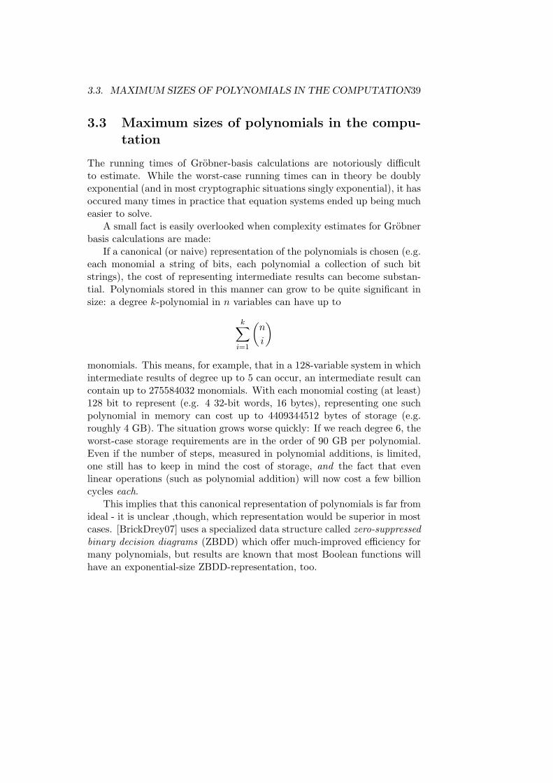
If a canonical (or naive) representation of the polynomials is chosen (e.g.each monomial a string of bits, each polynomial a collection of such bitstrings), the cost of representing intermediate results can become substan-tial. Polynomials stored in this manner can grow to be quite significant insize: a degree k-polynomial in n variables can have up to
k∑i=1
(n
i
)monomials. This means, for example, that in a 128-variable system in whichintermediate results of degree up to 5 can occur, an intermediate result cancontain up to 275584032 monomials. With each monomial costing (at least)128 bit to represent (e.g. 4 32-bit words, 16 bytes), representing one suchpolynomial in memory can cost up to 4409344512 bytes of storage (e.g.roughly 4 GB). The situation grows worse quickly: If we reach degree 6, theworst-case storage requirements are in the order of 90 GB per polynomial.Even if the number of steps, measured in polynomial additions, is limited,one still has to keep in mind the cost of storage, and the fact that evenlinear operations (such as polynomial addition) will now cost a few billioncycles each.
This implies that this canonical representation of polynomials is far fromideal - it is unclear ,though, which representation would be superior in mostcases. [BrickDrey07] uses a specialized data structure called zero-suppressedbinary decision diagrams (ZBDD) which offer much-improved efficiency formany polynomials, but results are known that most Boolean functions willhave an exponential-size ZBDD-representation, too.

Chapter 4
TheRaddum-Semaev-Algorithm
Most results in this chapter are the outcome of a cooperative meeting withMartin Albrecht and Ralf-Phillip Weinmann [Lesezirkel].
The Raddum-Semaev-Algorithm was introduced in [RadSem06] and wasable to solve some systems significantly faster than existing Grobner-Basisalgorithms. The paper is written from a computer-science perspective, whichmodels the problem of simultaneously solving a multivariate polynomialequation system as a problem of ’passing messages on a graph’.
The exposition which focuses on the graph obfuscates the algebraic-geometric meaning of the algorithm: It is much more intuitive to rep-resent the algorithm as a combination of projection of varieties to lower-dimensional spaces, intersecting such varieties, and then lifting the resultsto higher dimensions again.
In the following, the algorithm will first be explained along the samelines as the original paper did. After that, a more algebraic/geometric in-terpretation will be developed.
4.1 The original description
Let f1, . . . , fr ∈ Bn be the set of equations that are supposed to be solved.
Definition 4.1.1 (Variable Map). Let vars : Rn → P({x1, . . . , xn}) be amapping that maps a polynomial to the set of variables that occur in thispolynomial.
Definition 4.1.2 (RS-Assumption). Assume that |vars(fi)| <= k for somesmall k. This k needs to be small enough so that performing 2k evaluationsof fi is feasible, and storing r2k bit strings is feasible.
40

4.1. THE ORIGINAL DESCRIPTION 41
Data: Set of symbols S1 . . . SkResult: Set of symbols S′1 . . . S
′k
while last iteration deleted a configuration doforeach pair of symbols Si, Sj do
calculate Xij ;calculate Lij ∩ Lji;Delete configurations from Si, Sj that do not cover anyelement of Lij ∩ Lji;
endend
Algorithm 3: The agreeing algorithm
Definition 4.1.3 (Configuration). All solutions to fi can be represented aselements of F|vars(fi)|
2 , as only the values of variables occuring in fi need tobe stored. Such a vector is called a configuration.
Definition 4.1.4 (Symbol). A symbol (X,L) consists of an ordered set ofvariables X and a list L of configurations for X.
Definition 4.1.5 (Covering). Let X1 ⊆ X. A configuration for X is saidto cover a configuration for X1 if the two are equal for all variables in X1.
The core of the RS-Algorithm is the procedure called ’agreeing’. Con-sider Si, Sj and Xij = Xi ∩Xj .
Let Lij be the set of configurations for Xij that is covered by someconfiguration in Lj .
Let Lji be the set of configurations for Xij that is covered by someconfiguration in Li.
Two symbols agree if Lij = Lji
Remark 4.1.6 (Example:). Consider
S1 = ({x1, x2}, {10, 11})S2 = ({x1, x3, x4}, {011, 000, 101, 110})
Then Xij = {x1}, Lij = {1}, Lji = {0, 1}. The two symbols do not agree.We delete all configurations in S2 that do not cover any element in Lij∩Lji =
{1}. The result is S′2 =({x1, x3, x4},
101110
).
The authors interpret this algorithm as ’message passing on a graph’ –the individual equations form nodes on the graph, and the agreeing algo-rithm passes information about the solutions on one node to it’s neighboringnodes.
They note that the system of equations will often be in ’agreeing state’without showing a unique solution. They propose two ways of remedyingthe situation: Splitting and Gluing.

42 CHAPTER 4. THE RADDUM-SEMAEV-ALGORITHM
Splitting is performed as follows: If the agreeing algorithm fails to pro-duce a solution, an arbitrary symbol S is chosen. It is split into two halvesS′, S′′ by splitting the list of configurations into halves. The algorithm isre-run, once with S′ and once with S′′.
This step is the same as guessing that the solution lies in a particularhalf of the symbol under consideration, and running the algorithm on bothpossible guessed values.
Another step that can be taken to restart the agreeing step is gluing.Two symbols Si, Sj are chosen. Xi ∪ Xj =: X ′ is calculated. Then
the symbols Li, Lj are ’joined’ (through adding new configurations whereneeded).
Example:
S1 = ({x1, x2}, {01, 10})S2 = ({x1, x3, x4}, {100, 010, 011})
Then X ′ = {x1, x2, x3, x4}, L′ = {0110, 0111, 1000}. This can have negativeeffects on the size of a symbol though: In the worst case, the size of theresult is the product of the individual sizes:
|L′| = |L1||L2|
4.2 A geometric view
The RS-Algorithm can be much more easily understood as geometric oper-ations on the varieties. This helps in understanding under which conditionsthe algorithm will suceed in producing a solution. It will also be the basis onwhich the algorithm can be reinterpreted in terms of commutative algebrain the next section.
• The splitting step is simply a ’random cut’ of the variety into twovarieties of equal cardinality
• The gluing step is simply a ’union’ of two varieties
• The agreeing step is a combination of ’projection’, ’intersection’, and’lifting’. This is best illustrated with an example: Consider the twovarieties below. The variety on the left is defined over over F2[x, y, z],the one on the right is defined over F2[x, y, v].
zx
y
vx
y

4.3. AN ALGEBRAIC-GEOMETRIC VIEW 43
The varieties are projected to their common ’subspace’, e.g. theirprojection into F2[x, y] is calculated:
y y
The projections are intersected. This intersection is then lifted backto the two spaces from which the original varieties were projected:
y
zx
y
vx
y
The original varieties are intersected with this lifting. This eliminatespoints in each varieties that cannot be present in the other variety. Inour example, the first variety remains unchanged, whereas the secondhas the points highlighted in red removed:
zx
y
vx
y
4.3 An algebraic-geometric view
Through the previous geometric interpretation, the RS-algorithm can betranslated into the language of commutative algebra / algebraic geometry,making the comparison to other algorithms easier and allowing the algorithmto operate on polynomials instead of solution sets.
Definition 4.3.1 (Subspace Map). Let vars : Bn → P({x1, . . . , xn}) be amapping that maps a polynomial to the set of variables that occur in thispolynomial.
Let fi,j be the j-th monomial in fi. Then vars(fi) = vars(lcmj(fi,j)).
Definition 4.3.2 (Projection Map). ForM ⊆ {x1, . . . , xn}, let πM : P(Fn2 )→P(F#M
2 ) be the projection of the variety of a polynomial onto the smaller

44 CHAPTER 4. THE RADDUM-SEMAEV-ALGORITHM
subspace F#M2 corresponding to the subring RM := F2[mi]/〈m2
i + mi〉 ⊆Bn,mi ∈M .
Remark 4.3.3. A simple example is πvars(f)(V (〈f〉)) which maps the variety
of f into F#vars(f)2 - in essence, f is treated as a polynomial in the Ring of
Boolean functions that only contains the same variables as f . All in all,the projection map is just a technical construction – it doesn’t carry any“deeper” significance.
4.4 Raddum-Semaev Algorithm
The RS-Assumption is now reformulated using the above constructions:
Definition 4.4.1 (RS-Assumption). Assume that #vars(fi) < k for somesmall k. This k needs to be small enough so that performing 2k evaluationsof fi is feasible.
The entire algorithm can now be formulated in algebraic terms:
1. For each fi, the set vi := πvars(V (〈fi〉) is calulated. These are subsets
of F|vars(fi)|2 which correspond to what is called “configurations” in the
original formulation.
2. For each pair fi, fj , the set Sij := vars(fi) ∩ vars(fj) is calculated.
3. For each pair vi, vj , the set vij := πSij (vi) ∩ πSij (vj) is calculated -
exactly those points that agree on the smaller subspace F#Sij
2 . Thesepoints are then lifted back and intersected with vi, vj :
vi ← vi ∩ π−1Sij
(vij), vj ← vj ∩ π−1Sij
(vij)
This step is called the agreeing step in the original paper.
4. Once the agreeing has been run, the next step is called splitting. Thisdivides an arbitrary variety vi in two halves of equal cardinality andthen re-runs the algorithm on the two systems thus created. Thisessentially guesses ’which half’ of a variety a particular point is in.
5. New varieties are introduced in the step that the original paper calledgluing : Given a pair vi, vj , Uij = vars(fi) ∪ vars(fj) is calculated, andvi and vj are lifted to F#Uij
2 . Their intersection is calculated and formsa new variety vn. The agreeing step is run again.

4.4. RADDUM-SEMAEV ALGORITHM 45
4.4.1 Algebraization
Given 1.1.14 (intersecting varieties), 1.1.3 (unioning varieties), 1.1.7, theentire algorithm can be transformed to operate on polynomials in Bn insteadof sets of points. This eliminates the need to precompute solutions for allpolynomials and holding them in memory at all times (at the cost of havingto compute with potentially quite large polynomials).
The only thing that we are still missing in order to perform all operationsfrom the agreeing step directly on polynomials is the “projection to a smallersubspace”. But this can be easily achieved as follows:
Definition 4.4.2 (Projection). Let vars(f) = {x1, . . . xn}. Then
πvars(f)\{x1}(f) = f(0, x2, . . . , xn)f(1, x2, . . . xn)
We can hence recursively project larger polynomials to their restrictionson subspaces.
Gluing
The polynomial gluing step is even easier than the step performed on thelist of solutions: Since gluing corresponds to unioning varieties over thelarger space that is the union of the two spaces over which the varietieswere defined, this step can be simply implemented by multiplying the twopolynomials.
Splitting
The only step of the algorithm that cannot be trivially modeled to operateon polynomials is the splitting step, which randomly picks half the pointson a variety and then continues to run the algorithm.
Since we cannot (without exhaustive search over one intermediate poly-nomial) determine the full variety of such polynomial, we have multipleoptions to replace the splitting step.
1. Pick the polynomial f with a low number of variables and determineit’s variety by exhaustive search. Pick S ⊂ V (〈f〉) with cardinalityroughly half that of V (〈f〉). Then interpolate a new polynomial fromthis set of points by the following formula:
f ′ :=∑s∈S
(∏
x∈vars(f)
(x+ sx + 1) + 1)
This ensures that the new polynomial has exactly half the number ofsolutions that the previous polynomial had, but the cost of determiningall points is non-negligible.

46 CHAPTER 4. THE RADDUM-SEMAEV-ALGORITHM
2. Assume that the points of the variety of a given f are more or lessrandomly distributed. Then intersecting f with another polynomial gwhere #V (〈g〉) = 2#vars(f)−1 should, on average, yield a new polyno-mial with half the number of solutions. This other polynomial g mightbe a random linear polynomial, or a random quadratic polynomial, orwhichever polynomial that makes further calculations easy.
4.4.2 Summary
This chapter has put a geometric interpretation onto the RS-algorithm andprovided a bridge with which this algorithm can be reformulated as oper-ations on polynomials instead of operations on solution sets. While it isunclear whether this allows for any performance improvements, it shouldfacilitate comparisons to other algorithms of algebraic nature.
Furthermore, the geometric interpretation of the agreeing step showsthat it is particularly ill-suited for linear equations (the projection leads toan all-zero polynomial) – but fares quite well on many nonlinear ones.

Chapter 5
Published Algebraic attacks
One can argue, with some merit, that algebraic attacks have so far failed todeliver on their promise. Actual practical successes in breaking anything arefew and far between, and it has been argued that for each algebraic attackon a block cipher, a more efficient statistical attack has been found.
On the other hand, a possible explanation for the disenchantment withalgebraic attacks is the disappointment after having built unrealistic expec-tations: Extremely optimistic claims about the efficiency of algebraic attackswere publicly made in the past, and high hopes generated (“cryptanalysisusing only one plain/ciphertext pair”, “solving very overdefined systems isgenerally polynomial in nature” etc.). With such hype, it was nearly impos-sible for algebraic methods to live up to expectations.
In essence, successes of algebraic cryptanalysis have been limited toLFSR-based stream ciphers and asymmetric multivariate schemes (such asHFE).
In the following, a few of the published algebraic attacks will be dis-cussed, and what the author perceives to be the “crucial” point that helpedmake the attack successful.
The algebraic attacks that were published so far are, overall, quite sim-ilar in nature: An equation system for the cipher in question is generated,some preprocessing is performed on the generated equations, and an attemptto solve the equation system is made. The attempt to solve the equationsystems is usually done via either a Grobner-basis calculation (using moreefficient algorithms such as F4 or F5) or via relinearization.
Interestingly, it appears that “naively” generated equation systems arealmost always beyond the abilities of common equation system solvers, bethey Grobner-basis calculations or relinarizations. The crucial step seemsto be the “preprocessing” of equations.
47

48 CHAPTER 5. PUBLISHED ALGEBRAIC ATTACKS
5.0.3 Lowering the degree by multiplication
The first idea put forward in [CourMeier] and [Armknecht] is lowering thedegree of the equations that are collected by multiplying them with well-chosen other polynomials.
In [CourMeier], several separate scenarios are discussed:
S3a There exists a function g of low degree such that fg = h with h 6= 0and of low degree
S3b There exists a function g of low degree with fg = 0
S3c There exists a function g of high degree such that fg = h where h 6= 0and of low degree.
The paper [MeiPaCar] goes on to show that in reality only two scenarios,namely S3a and S3b need to be considered. This thesis will give an alternateinterpretation of the above scenarios in 6.4.2 .
Summary
The crucial idea here is that the degree of polynomials f1, . . . , fr can some-times be lowered by multiplying them with another polynomial. Multiplyingour fi with other polynomials does not risk “losing” solution points: If fi isin the ideal generated by 〈f1, . . . , fr〉, then so is fig. Geometrically, we’reonly “adding” points.
5.0.4 Lowering the degree by finding linear combinations
Another idea was put forwards in [CourFast]: If the collection of equa-tions and the subsequent multiplication with well-chosen polynomials stilldoes not yield sufficiently low degree, linear combinations of these equationsmight be found that do.
In the context of stream ciphers, [Armknecht] describes the conditionsunder which such an attack works as follows:
• The equation system has been set up by use of an r-Function, e.g. isof the form:
F (X1, . . . , Xr, z1, . . . , zr) = 0. . . . . .
F (Xn−r, . . . , Xn, zn−r, . . . , zn) = 0
• The r-Function F can be rewritten so that
F (X1, . . . , Xr, z1, . . . , zr)︸ ︷︷ ︸deg(F )=d
= G(X1, . . . , Xr)︸ ︷︷ ︸degG=d
+H(X1, . . . , Xr, z1, . . . , zr)︸ ︷︷ ︸deg(H)<d

49
According to [Armknecht], the ciphers E0, Toyocrypt and LILI-128 allsatisfy this condition.
In such a situation, the equation system will look like
G(X1, . . . , Xr) +H(X1, . . . , Xr, z1, . . . , zr) = 0G(X2, . . . , Xr+1) +H(X2, . . . , Xr+1, z2, . . . , zr+1) = 0
. . . = . . .
G(Xn−r, . . . , Xn) +H(Xn−r, . . . , Xn, zn−r, . . . , zn) = 0
For shorter notation, rewrite G(X1+i, . . . , Xr+i) as Gi.Since G is bounded to be of degree ≤ d, there are “only” µ(n, d) =∑di=0
(nd
)different monomials that can occur. As a consequence, any se-
quence of Gi of length ≥ µ(n, d) has to be linearly dependent, e.g. thereexist coefficients λ1, . . . , λµ(n,d) so that
∑µ(n,d)i=1 λiGi = 0.
This alone would already yield equation systems of lower degree: Thesum
µ(n,d)∑i=1
λiF (X1+i, . . . , Xr+i)
would have lower degree than the original equations.But the situation is even better: It can even be shown that Gi is a
linear recurring sequence. The following is taken almost verbatim from[Armknecht]:
Lemma 5.0.3. The sequence Gi forms a linear recurring sequence. Thismeans that there is some integer T so that
T∑i=0
λiGt+i = 0 ∀t ≥ 0
The minimal polynomial of the linear recurring sequence can be calcu-lated by a modified version of the Berlekamp-Massey algorithm.
Summary
The important idea here is that given a system f1, . . . , fr of equations, ele-ments can be added freely without “losing” any solution points: Arbitrarylinear combinations of ideal generators stay in the same ideal. As such, anylinear combination that transforms f1, . . . , fr into something that is morenicely behaved with respect to the eventual equation system solver is quiteuseful.

50 CHAPTER 5. PUBLISHED ALGEBRAIC ATTACKS
5.0.5 Faugere-Ars attack on nonlinear filters
In [FaugArs03], the authors describe how they attacked nonlinear filter gen-erators using Grobner bases. No special preprocessing was mentioned – theauthors simply generated equation systems from nonlinear filters and cal-culated Grobner bases using F5. According to the paper, they were able torecover the full state of the underlying LFSR given Ld output bits (whereL is the number of unknown bits in the LFSR and d the degree of thecombining polynomial).
5.0.6 Experimental attack on Toyocrypt
An experimental attack that combines the techniques described in [CourMeier]and Grobner basis algorithms has been carried out in [KaImWa]. The au-thors combined the technique of lowering the degree of the equation systemwith their own implementation of the F4 Grobner base algorithm. This wasdone in 3 steps:
1. Equations were generated and their degree was lowered using 5.0.3
2. Using Berlekamp-Massey, relations between the equations to furtherlower the degree were calculated
3. The resulting equation system was fed into a parallelized version of F4
The second step took 10+ hours, but the result was an equation systemwhich, according to the authors, could be solved in 20 seconds.
5.1 The notion of algebraic immunity
As a reaction to [CourMeier], criteria for judging the resilience of Booleanfunctions against algebraic attacks were proposed. The principal definitionin use nowadays appears to be the following:
Definition 5.1.1 (Algebraic Immunity). The algebraic immunity of f ∈ Bnis the minimal degree d of a function g ∈ Bn so that fg = 0 or (f + 1)g = 0.Formally:
AI(f) := min{deg(g)|g ∈ Bn, fg = 0 ∨ (f + 1)g = 0}
The use of the name algebraic immunity is under debate though: [Armknecht]prefers to call it annihilator immunity, as algebraic immunity seems to im-ply resistance against a wide variety of algebraic attacks. This is not thecase: The only thing that algebraic immunity implies resistance against arethe degree-lowering tricks discussed in 5.0.3, and through that a certain re-sistance against Grobner-basis calculations (as these usually take longer forhigher-degree equation systems).

Chapter 6
The Pseudo-EuclidianAlgorithm
This chapter discusses the actual ’meat’ of the present thesis: A new equa-tion system solving algorithm specialized to F2 and some of its properties.
The result of Lemma 1.1.14 establishes that Bn is a principal ideal ringand also provides a constructive method to calculate the single generator ofan ideal from a set of generators in 1.1.16, mimicking the behavior of theEuclidian algorithm in Euclidian rings.
Given a set of generators g1, . . . , gn with V (〈g1, . . . , gn〉) = {y}, y ∈ Fn2 ,we know the exact form of the generator g through the result of 1.1.6. Therestricted form of g allows us to ’read off’ the single-point solution y inquestion.
The result is an algorithm that will, given a system of multivariate poly-nomial equations over F2 which have exactly one common solution, producethe solution to a given set of n equations in n + 1 additions in Bn and nmultiplications in Bn.
This sounds exciting, but at the same time we know that the mentionedproblem is NP-hard - we therefore know that we have exponential complexityhiding somewhere in the above (it turns out it’s hiding within multiplicationsin Bn).
6.0.1 A naive first algorithm
Let G be a set of polynomials g1, . . . gk ∈ Bn and 〈g1, . . . , gk〉 the idealgenerated by these polynomials in Bn. Furthermore, assume that the varietyof the ideal consists of exactly one point, e.g. |V (〈g1, . . . , gn〉)| = 1.
One can make use of the results 1.1.7 and 1.1.14 in order to compute thesingle point on the variety.
Remark 6.0.2. One can use 1.1.16 to calculate g ∈ Bn with G := V (〈g〉) =V (〈g1, . . . , gn〉).
51

52 CHAPTER 6. THE PSEUDO-EUCLIDIAN ALGORITHM
Remark 6.0.3. The variety G consists of only one point. It is thus in theintersection of the variety V (〈x1〉) with some other set H ⊂ Fn2 or in theintersection of the variety V (〈x1 + 1〉) with some other set H ⊂ Fn2 . G canalways be ’decomposed’ in one of the two following ways:
1. ∃H ⊂ Fn2 so that G = V (〈x1〉) ∩H
2. ∃H ⊂ Fn2 so that G = V (〈x1 + 1〉) ∩HLemma 6.0.4. Let g be so that G = V (〈g〉). For any i exists h ∈ Bn sothat
g = xi + h+ hxi or g = xi + 1 + hxi
Proof. Let G ⊂ V (〈xi〉) ⇔ G = {y} with yi = 0. Then there exists aH ⊂ Fn2 so that G = H ∩ V (〈xi〉), and from 1.1.14 it follows that if h ∈ Bnwith V (〈h〉) = H, then
g = xi + h+ hxi
Let G ⊂ V (〈xi + 1〉) ⇔ G = {y} with yi = 1. Then there exists a H ⊂ Fn2so that G = H ∩ V (〈xi + 1〉), and from 1.1.14 it follows that if h ∈ Bn withV (〈h〉) = H, then
g = (x1 + 1) + h+ h(x1 + 1) = x1 + 1 + h+ hx1 + h = x1 + 1 + hx1
Lemma 6.0.5. Given g, one can easily test for the individual componentsof y:
1. Test whether (xi + 1) | (g + xi) ⇒ yi = 0
2. Test whether xi | (g + 1 + xi) ⇒ yi = 1
Proof. Let g = xi + h+ hxi ⇔ g + xi = h(xi + 1). But g = xi + h+ hxi isequivalent to yi = 0.
Let g = xi+1+hxi ⇔ g+xi+1 = hxi. But g = xi+1+hxi is equivalentto yi = 1.
So in summary, one calculates a generator g then tries to decompose itin intersections of univariate linear polynomials in order to determine thevalues of the individual components of the solution.
We can see from the above algorithm that once we have calculated g wecan pretty much determine it’s (single-point) solution in linear time.
The difficulty (and computational complexity) is hidden in the calcula-tion of g. If we follow 1.1.16, we need n polynomial multiplications and n+1polynomial addition.
With each polynomial multiplication, the number of monomials can growto the product of the numbers of monomials of the factors, e.g. if |f | and|g| denote the number of monomials in f resp. g, then |fg| ≤ |f ||g| in theworst case.

6.1. SOME EMPIRICAL DATA 53
6.1 Some empirical data
6.1.1 Hard instances of MQ
In order to put the algorithm to the test, a mail was sent to JC Faugereasking for a good way to generate equation systems that are difficult to solveusing Grobner base algorithms. His reply was:
From the Groebner Basis computation point of view the mostdifficult case is to consider a system of random quadratic equa-tions:Let g1(x11, . . . , xn), . . . , gn(x1, . . . , xn) where gi is random and
deg(gi) = 2
Then select randomly (a1, . . . , an) ∈ Fn2 . Then try to solve thealgebraic system S = {f1(x1, . . . , xn), . . . , fn(x1, . . . , xn)} wherefi(x1, . . . , xn) = gi(x1, . . . , xn)− gi(a1, . . . , an).S has in general one solution.
From experimentation, it is presumed that in the above the number ofequations should outnumber the number of variables - at least empirically,single-solution systems were only generated about 50% of the time if n wasboth the number of unknowns and equations.
This is not surprising: Empirically, each random quadratic polynomialin n variables has as variety a more or less random subset of Fn2 with ap-proximately 2n−1 points. A system of k such equations has as solution setthe intersection of k such sets. This means that for each point, the odds ofthis point “being a solution” are roughly 1
2k . At the same time, we have 2n
points.
The experiment
The following experiment was conducted:
1. 20000 overdefined systems with 15 unknowns and 28 equations de-scribing the system were generated. These systems were constructedso that they have randomly chosen single-point varieties. 1.1.13 tellsus that the size of the final polynomial in the last step of the algorithmwill be 2l where l is the number of zero-bits in the solution.
2. The algorithm was run on each of these systems. After each step ofintersection, the number of monomials in the intermediate polynomialwas recorded
3. Once all equations had been processed, the result (e.g. the solution)was read off and verified to be correct

54 CHAPTER 6. THE PSEUDO-EUCLIDIAN ALGORITHM
4. The process was repeated with 20000 similar equation systems that, in-stead of a random single-point solution, the fixed solution of (1, . . . , 1).This was done because the number of monomials in the final equationdepends on the number of 0-entries in the solution vector - as such,setting all solutions to a fixed known value should eliminate fluctu-ations in intermediate results that are due to the nature of the finalresult.
The following observations were made:
1. For almost all equation systems, the maximum number of monomialsin the intermediate polynomial did not exceed 2n−1 = 214. In the testset of 20000 random-solution equations, 500 exceeded the 214 bound-ary, accounting for 2.5% of the total number of systems that weregenerated.
2. No equation system stayed below 13273 monomials in the intermediatepolynomial during all steps of the algorithm. This means that whileonly 2.5% exceeded the size of 2n−1 = 214 monomials, all equationsystems exceeded the size of 2n−2 = 213 monomials.
3. 98.65% of all equation systems had their maximum intermediate poly-nomial size before the seventh intersection. 95.255% of all equationsystems had their maximum intermediate polynomial size before thesixth intersection. 46.72% of the equation systems had their maximumintermediate polynomial size at exactly the fourth intersection.
Figure 6.1: The number of monomials at each step in the algorithm for2000 randomly generated systems. The blue line denotes the 214 monomial-boundary. Each curve is drawn transparently to help identify ’density’.
6.2. GETTING OTHER INFORMATION ABOUT THE VARIETY 55
Observations and Conclusion
As expected, we encounter exponential growth in running time and mem-ory complexity. The size of the intermediate polynomials explodes - andthrough this, the cost of performing polynomial multiplication. It is inter-esting to see that the algorithm looks cheap on paper only because no properboundaries on the sizes of the intermediate results are given – this appearsto imply that in any complexity analysis for equation system solvers, thesize of the intermediate results is no less important than the total numberof calculations involved.
6.1.2 Equation systems generated from cryptographic prob-lems
In previous chapters, it became evident that constructing full equation sys-tems for PRESENT is infeasible without introducing spurious quantities ofintermediate variables. As result of this, only severely weakened variants ofthe cipher could be investigated here. Outside of the difficulty of generatingequation systems, solving was an entirely different issue - many equationsystems that could be generated could not be solved without running out ofmemory.
Solving more than 2 rounds failed with the full cipher, and even weak-ening the cipher to 40 bits did not allow more than 2 rounds to be solvedwithout exceeding 4 GB of memory consumption. Only the extreme mea-sure of weakening the cipher to 20 respective 16 bit allowed for the algorithmto run in reasonable time.
From our experience with truly hard MQ-instances, we should expectthe intermediate polynomials to grow to a size between 215 and 219 mono-mials. We can see in the following diagram that this was achieved for 20-bitPRESENT in round 5, but not for 16-bit PRESENT.
One oddity arises in the equations generated from 5 rounds of 20-bitPRESENT: The complexity peak is much earlier than for 4 rounds, anddrops off quite sharply: After taking 12 equations into account, the com-plexity of the intermediate results is consistently lower than the intermediateresults for 4 rounds. A good explanation for this is, unfortunately, not avail-able.
6.2 Getting other information about the variety
6.2.1 Determining equality between variables
The algorithm 6.0.5 tries to determine properties of the variety of a mul-tivariate polynomial f ∈ Bn by attempting to split the polynomial in twopolynomials - one of which has an easily-understood variety. In 6.0.5 the

56 CHAPTER 6. THE PSEUDO-EUCLIDIAN ALGORITHM
Figure 6.2: Sizes of the intermediate polynomials while solving 4 (red) re-spective 5 (orange) rounds of PRESENT weakened to 16 bits. The sizepeaks at 11925 monomials for 4 rounds and 25805 monomials for 5 rounds.A peak around 32768 would be expected for random systems. This seemsto imply that after 5 rounds, the hardness of truly random systems is notachieved yet. 1 square = 1000 monomials
Figure 6.3: Sizes of the intermediate polynomials while solving 4 (red) re-spective 5 (orange) rounds of PRESENT weakened to 20 bits. The size peaksat 209735 monomials for 4 rounds and 512513 monomials for 5 rounds. For5 rounds, this is quite close to the 524288 monomials that would be expectedof a truly random system. 1 square = 10000 monomials

6.3. VIEWING THE ALGORITHM AS TRAVERSAL OF A LATTICE57
’simple’ polynomials (xi+1, xi) had ’half-spaces’ as varieties, but this is nota necessity. It is possible to ask comparatively complicated questions suchas ’is the first variable always equal to the second variable in each point inthe solution ?’ by applying the same principle.
In order to determine wether a given polynomial g has above-mentionedproperty, we attempt to decompose g as follows:
g = (x1 + x2) + h+ h(x1 + x2) = x1 + x2 + h+ hx1 + hx2
⇔ g + x1 + x2 = h(1 + x1 + x2)
This leads us to a simple test for said property that can be evaluatedvia a simple multivariate polynomial division.
6.2.2 Monomial count and hamming weight
A trivial corollary of 1.1.13 is that even if we end up not being capableof calculating f explicitly, other things can give us information about thesolution of the equation system:
If we can calculate the number of monomials in f , or even approximatethe number of monomials in f with reasonable error boundaries, we candeduce boundaries on the hamming weight of the solution vector.
6.2.3 Attempting solutions without calculating the product
An interesting factoid was pointed out by L. Gerritzen:
Lemma 6.2.1. Let f ∈ Bn with exactly one solution (y1, . . . , yn) ∈ Fn2 .Then yi = 0⇔
∏nj=0,j 6=i xj is a monomial in f .
Proof. Follows from the proof of 1.1.13 with a small amount of effort.
This implies that it if we were capable of testing for presence of a partic-ular monomial in
∏ni=1(fi + 1)) + 1, we are able to determine the hamming
weight of the solution.
6.3 Viewing the algorithm as traversal of a lattice
Warning: The word “lattice” is overloaded. The meaning that is used hereis the order-theoretic one !
The pseudo-Euclidian algorithm presented above can be interpreted asthe traversal of a particular lattice. There are several ways to interpret thelattice.

58 CHAPTER 6. THE PSEUDO-EUCLIDIAN ALGORITHM
Set-theoretic interpretation
The algorithm can be interpreted as a traversal of the lattice formed byP(Fn2 ) with the operations ∪,∩. Given the system of equations f1, . . . , fn onelooks at V (f1), . . . , V (fn) ∈ P(Fn2 ) and then iteratively calculates
⋂ni=1 V (fi).
Coordinate-Ring interpretation
An alternative view of the algorithm is as the iterated construction of co-ordinate rings over Bn along with projection mappings. The algorithm canbe interpreted as constructing a series BF i = BF i−1/〈fi−1〉,BF1 := Bn andmappings φi : BF i−1 → BF i:
Bn →︸︷︷︸φ1
BF1 → . . . →︸︷︷︸φn−1
BFn−1
as well as f := φ1 ◦ · · · ◦ φn−1(fn).By calculating fij = (fi + 1)(fj + 1) + 1 = fi + fj + fifj , one effectively
projects fi into Bn/〈fj〉 (or, equivalently, fj into Bn/〈fi〉).
Commonalities
Wether the algorithm is viewed as a traversal of the powerset-lattice of Fn2or as the traversal of the lattice of coordinate rings is irrelevant since bothlattices are isomorphic in this case. The important points are:
1. Initially, one starts with a set of lattice elements f1, . . . , fn
2. One can incrementally calculate fi ∧ fj for pairs of points
3. The goal is to calculate∧ni=1 fi
4. Some elements of the lattice are very expensive to represent, othersare cheap to represent.
5. The order in which the calculation happens corresponds to a traversalof the lattice.
A small example
In order to clarify the above, consider a small example. Let
f1 := y + xy, f2 := x+ y + xy + 1, f3 := x+ y + 1
We identify polynomials in B2 with their subsets in P(F22) and draw the
resulting lattice (the varieties of f1, f2, f3 have been highlighted):

6.3. VIEWING THE ALGORITHM AS TRAVERSAL OF A LATTICE59
∅
{(00)}
{(01)}
{(10)}
{(11)}
{ (00)(01)
}
{ (00)(10)
}
{ (01)(10)
}
{ (00)(11)
}
{ (01)(11)
}
{ (10)(11)
}
{(00)(01)(10)
}
{(00)(01)(11)
}
{(00)(11)(10)
}
{(10)(11)(01)
}
F22
Instead of set notation, one can also label the lattice elements with theircorresponding polynomials. The polynomials f1, f2, f3 are highlighted:
1
x+ y + xy
x+ xy + 1
y + xy + 1
xy + 1
y
x
x+ y + 1
x+ y
x+ 1
y + 1
xy
y + xy
x+ xy
x+ y + xy + 1
0
There are 3 different ways of calculating∧3i=1 fi: (f1 ∧ f2) ∧ f3, (f2 ∧
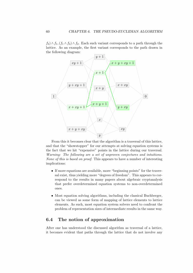
60 CHAPTER 6. THE PSEUDO-EUCLIDIAN ALGORITHM
f3)∧ f1, (f1 ∧ f3)∧ f2. Each such variant corresponds to a path through thelattice. As an example, the first variant corresponds to the path drawn inthe following diagram:
1
x+ y + xy
x+ xy + 1
y + xy + 1
xy + 1
y
x
x+ y + 1
x+ y
x+ 1
y + 1
xy
y + xy
x+ xy
x+ y + xy + 1
0
From this it becomes clear that the algorithm is a traversal of this lattice,and that the “showstopper” for our attempts at solving equation systems isthe fact that we hit “expensive” points in the lattice during our traversal.Warning: The following are a set of unproven conjectures and intuitions.None of this is based on proof. This appears to have a number of interestingimplications:
• If more equations are available, more “beginning points” for the traver-sal exist, thus yielding more “degrees of freedom”. This appears to cor-respond to the results in many papers about algebraic cryptanalysisthat prefer overdetermined equation systems to non-overdeterminedones.
• Most equation solving algorithms, including the classical Buchberger,can be viewed as some form of mapping of lattice elements to latticeelements. As such, most equation system solvers need to confront theproblem of representation sizes of intermediate results in the same way.
6.4 The notion of approximation
After one has understood the discussed algorithm as traversal of a lattice,it becomes evident that paths through the lattice that do not involve any

6.4. THE NOTION OF APPROXIMATION 61
’expensive’ points are desirable. This leads directly to the question of ap-proximation:
Given an ’expensive’ polynomial, can we approximate it through a ’cheap’polynomial ?
Before tackling this question in any depth, it is first necessary to clarifythe notion of ’cheap’, ’expensive’, and ’approximation’:
Definition 6.4.1 (Cost function). A mapping φ : Bn → R that, in someform, encodes the ’cost’ of representing (or working with) a particular Booleanfunction, is called a cost function
Examples of cost functions:
• φV : Bn → N ⊂ R, φV (f) 7→ |V (f)|. As one can represent a Booleanfunction by its variety, this function measures the cost of representingthe function by explicitly storing all points of the variety.
• φM : Bn → N ⊂ R, φM (f) 7→ |{m Monomial of f}|. One can representa Boolean function by the set of monomials. This function measuresthe cost of doing so by counting the number of monomials in f .
• φV OBDD : Bn → N ⊂ R
φV OBDD(f) 7→ |{v, v Node in the OBDD-representation of V (f)}|
The variety might be more compactly represented as OBDD, thereforeit makes sense to know the cost of representing a function in thismanner.
• φOBDD : Bn → N ⊂ R
φOBDD(f) 7→ |{v, v Node in the OBDD-representation of f}|
. Likewise, the set of monomials might be more compactly representedas OBDD, so the size of the OBDD-representation of the set of mono-mials is a cost function, too.
6.4.1 Approximation of polynomials
Now that cost functions are in place, a clear definition of approximationis needed. Intuitively, an approximation g of f is a function that differson a small number of points from f . One can think of overapproximations(e.g. g vanishes on more points than f) and underapproximations (e.g. gvanishes on fewer points than f), which form subclasses within the set ofapproximations. The quality of an approximation is measured as the numberof points on which the two functions differ, e.g. their hamming distance.Given f and g, we can easily calculate a polynomial that vanishes exactlyon the points where f and g differ: f + g + 1.

62 CHAPTER 6. THE PSEUDO-EUCLIDIAN ALGORITHM
Definition 6.4.2 (φ-Approximation of quality k). Let φ be a cost function.A polynomial g ∈ Bn is called a φ-approximation of quality k if |V (f + g +1)| = k and φ(g) < φ(f). This means that g is cheaper to represent than f ,but differs from f at only k points.
Definition 6.4.3 (φ-Overapproximation of quality k). A polynomial g ∈ Bnis called a φ-overapproximation of f ∈ Bn with quality k if |V (f + g+ 1)| =k, V (f) ⊆ V (g) and φ(g) < φ(f). This means that g is cheaper to representthan f and vanishes at k points at which f doesn’t vanish. This is the sameas stating that g’s variety is the same as f ’s variety with k points added.
Definition 6.4.4 (φ-Underapproximation of quality k). A polynomial g ∈Bn is called a φ-underapproximation of f ∈ Bn with quality k if |V (f + g +1)| = k, V (g) ⊆ V (f) and φ(g) < φ(f). This means that g is cheaper torepresent than f and does not vanishes at k at which f vanishes. This isequivalent to stating that g’s variety is f ’s variety with k points removed.
A number of small corollaries follow immediately:
Corollary 6.4.5. The set of all overapproximations {g1, . . . , gk} ⊂ Bn off ∈ Bn is isomorphic to the ideal generated by f .
This follows from the fact that multiplying two polynomials results inthe union of their varieties, and the fact that for all g the statement fg ∈ 〈f〉holds.
Corollary 6.4.6. There is a bijection between the set of all underapproxi-mations {g1, . . . , gn} ⊂ Bn of f ∈ Bn and the elements of the ideal of f + 1.
This follows because each underapproximation g yields an overapproxi-mation g + 1 of f + 1.
6.4.2 Re-visiting Courtois-Armknecht attacks on stream ci-phers
One of the few successes of algebraic cryptanalysis were the Courtois-Armknechtattacks on stream ciphers. The principal trick that was responsible for low-ering the degree of the equation systems far enough to make them solublewas, for given f1, . . . , fn finding polynomials g so that f1g, . . . , fng had muchlower degree.
With the above constructions, one sees now that the “degree-lowering”trick employed in [Armknecht], [CourMeier] (and described here in 5.0.3) isnothing different than finding overapproximations fg of low degree. Thisraises an interesting question that has not been treated in the literature:
Since lowering the degree of equations f1, . . . , fn consists of multiplyinga polynomial with each of them, one effectively adds points to each variety.

6.4. THE NOTION OF APPROXIMATION 63
If the same polynomial is used for all equations, one even adds the samepoints to each variety.
This has implications for the solution set: The uniqueness of the solutionmight be lost. At the very least adding points to our solution sets mightmean that more equations are needed before the solution becomes unique.
There is another, less clear-cut risk, too, although it seems to not havehappened in practice: If one adds the same additional solutions to eachequation, solving will of course become much easier - at least the pointsthat we added to all equations will be a solution for the entire system,albeit not the one we were looking for. One should keep in mind that theso-called “pre-processing”-steps might have an influence on the solution set(e.g. enlarge the solution set).
Corollary 6.4.7. The r-Functions described in [Armknecht] are a form ofapproximation:
Recall the definition of an r-function: Given a (ι,m)-combiner and afixed r, a function F is an r-function for the combiner if
F (X1, . . . , Xr, y1, . . . , yr) = 0
holds whenever X1, . . . , Xr and y1, . . . , yr are successive inputs respectiveoutputs of the output function χ.
This r-function is an overapproximation for the full equation system gen-erated by the combiner: All valid “solutions” X to the equation system
zt = χ(Sm,t,KLtP )
with appropriate equations to model Sm,t as result of Sm,t−1 and KLt−1Palso satisfy F (X) = 0. Therefore an r-function is an overapproximation ofthe equation system generated by multiple clocks of the combiner.
In response to the published algebraic attacks, the notion of algebraicimmunity was introduced (see 5.1.1.
Corollary 6.4.8. Algebraic immunity is is a criterion about nonexistenceof overapproximations of low degree. It states that no overapproximationsin regard to φ = deg exist.
Generalisation of degree-lowering techniques
After looking at 5.0.4 and 5.0.3, it is difficult not to make a generalization:Multipliying fi with a polynomial g is a valid operation on our equation
system: Geometrically, we’re just adding solutions, algebraically, we remainin the same ideal. Creating linear combinations of fi is a valid operationon our equation system: Geometrically, V (fi) ∩ V (fj) ⊆ V (fi + fj), e.g.the intersection of two varieties is a subset of the variety of the sum, andalgebraically the sum is part of the same ideal.

64 CHAPTER 6. THE PSEUDO-EUCLIDIAN ALGORITHM
It is therefore clear that any operation on the equation system thatremains in the ideal in question is legitimate. This leads to a generalizednotion of degree-lowering-tricks:
Definition 6.4.9 (Degree-Lowering-Polynomial). Let
〈f1, . . . , fr〉 ⊆ F[x1, . . . , xn] =: R
be an ideal. An element h ∈ R[y1, . . . , yr] is a degree-lowering polynomial if
deg(h(f1, . . . , fr)) ≤ min{deg fi|i = 1, . . . , r}
In essence, it is a polynomial with coefficients in F[x1, . . . , xn] so thatwhen all fi are substituted for yi, the resulting polynomial has lower degreethan any fi.
One sees easily that 5.0.3 means that the degree-lowering polynomial hasonly one monomial, e.g. is of the form h := gy1 (where g is the polynomialthat our equation is multiplied with). One also sees easily that 5.0.4 usesdegree-lowering polynomials that are linear, e.g. of the form h :=
∑i∈I yi.
A first idea to calculate such h would be to use Grobner bases: If oneproceeds similarly to 5.0.4 and splits the fi into high-degree components Giand low-degree components Hi, one could attempt to calculate the syzygymodule of the Gi. This would yield polynomials in R that evaluate tozero if the Gi are inserted. Unfortunately, things are not quite so easy: Inthe case of a linear h, calculating h(G1 + H1, . . . , Gr + Hr) does not yieldany interaction between the high-degree and low-degree components: If thehigh-degree parts cancel, only low-degree parts are left. In case of generalpolynomials for h, this is no longer the case: Several low-degree componentsmight be combined to yield high-degree results, and complicated interactionsoccur. It is, as of now, wholly unclear how a good h might be constructed.
While not being very constructive, this definition allows us to define ageneralized algebraic resistance (with respect to deg):
Definition 6.4.10 (Generalized algebraic resistance (with φ = deg)). Asystem of equations
f1, . . . , fr
is has generalized algebraic resistance (with φ = deg) of d where
d = min{deg(h(f1, . . . , fr)), h ∈ R[y1, . . . , yr]}
From an algebraic perspective, this definition is equivalent to
d = min{deg(f), f ∈ 〈f1, . . . fr〉}
Looking at the situation from this angle, we see an amusing corolary:

6.4. THE NOTION OF APPROXIMATION 65
Corollary 6.4.11. Any system F := 〈f1, . . . , fr〉 ⊆ Bn with unique solutionin Bn satisfies d = 1.
Proof. We know that any polynomial that has a superset of V (F ) as varietyis an element of F . Therefore, either the polynomial x1 or the polynomialx1 + 1 is an element of F , and d = 1.
This means that as long the system of equations has unique solution,there will be an h so that the degree of the system can be lowered, evento 1. In order to have a more meaningful measure of resistance, one wouldneed to take more things into account, at least the following:
1. The cost of calculating h(F1, . . . , Fr)
2. The “loss of accuracy” when calculating h
6.4.3 Constructing approximations
Since the problems we ran into during the solving of our equation systems us-ing the pseudo-Euclidian algorithm had little to do with degree, and muchmore to do with exponential growth in the number of monomials in ourintermediate results, a natural question arises: Can we construct an over-approximation g for a given large polynomial f in a systematic fashion ?
A first stab
Without loss of generality, let f contain the monomial ’1’. Let l be thenumber of monomials in f . The goal is now to construct g ∈ Bn withgf = g ⇔ f(g + 1) = 0 so that the number of monomials m of g are lessthan or equal l.
We fix m < l. Let fi denote the i-th monomial of f with some ordering,and let gi denote the i-th monomial of g with some ordering.
The standard way of multiplying f with g works by filling in the elementsof the following matrix and removing all matrix elements that occur an evennumber of times:
f1 . . . fl−1 1g1 f1g1 fl−1g1 g1. . .gm f1gm fl−1gm gm
In order to satisfy the condition that fg = g, it has to be assured thatall matrix elements except the right-most column occur an even number oftimes.
The algorithm now works as follows: The above matrix is consideredwithout the rightmost column. It’s elements are called a1, . . . , al−1,m. Anarbitrary decomposition into disjoint subsets of cardinality 2 is chosen (there

66 CHAPTER 6. THE PSEUDO-EUCLIDIAN ALGORITHM
are k!k2!2
k2
possible such decompositions for sets of cardinality k when 2 divides
k). Each such “pair” needs to “cancel”, e.g. both elements of the pair haveto be equal. Thus each subset of cardinality 2 of matrix elements of theform {ai, aj} gives rise to an equation of the form ai = aj . This is the sameas
fαgβ = fγgδ
for some α, β, γ, δ. This implies log(fαgβ) = log(fγgδ). Since multiplica-tion of monomials is the same as bit-wise “or” of the exponents, and sincexORy = x+ y + xy, the following system of equations arises:
log(fα)1 + log(gβ)1 + log(fα)1 log(gβ)1 = log(fγ)1 + log(gδ)1 + log(fγ)1 log(gδ)1. . . = . . .
log(fα)n + log(gβ)n + log(fα)n log(gβ)n = log(fγ)n + log(gδ)n + log(fγ)n log(gδ)n
This would normally look like a rather large linear equation system (withnm unknowns), but because the log(fi) are all known, only the followingfour types of equations can arise:
log(fα)i = 0 = log(fγ)i ⇒ log(gβ)i = log(gδ)i (6.1)log(fα)i = 0, log(fγ)i = 1, ⇒ log(gβ)i = 1 (6.2)log(fα)i = 1, log(fγ)i = 0, ⇒ log(gδ)i = 1 (6.3)
log(fα)i = 1 = log(fγ)i ⇒ 0 = 0 (6.4)
This means that each equation can either imply equality between twoparticular exponents in the monomials gβ and gδ, or that one of the twomonomials needs to have a particular exponent set to 1. Interestingly, thisalso implies that the equation system will always have a solution: Since thereis no way that a value of 0 can be implied, there is no way a contradictioncould arise. This is not surprising: the polynomial g = 0 will always be anoverapproximation to f (but of little value).
The above thoughts lead to the following algorithm that constructs a“random” overapproximation of f :
Data: f ∈ Bn,m ∈ NResult: g ∈ Bn with fg = g and φM (g) = minit;g ← 0;while g == 0 do
choose random partition;generate system of equations;solve for g;
endReturn g;
Algorithm 4: Approximation of polynomials
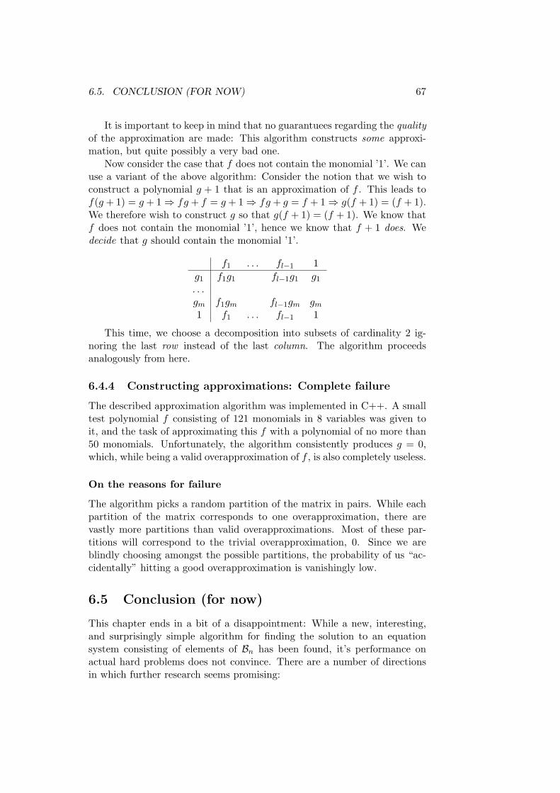
6.5. CONCLUSION (FOR NOW) 67
It is important to keep in mind that no guarantuees regarding the qualityof the approximation are made: This algorithm constructs some approxi-mation, but quite possibly a very bad one.
Now consider the case that f does not contain the monomial ’1’. We canuse a variant of the above algorithm: Consider the notion that we wish toconstruct a polynomial g + 1 that is an approximation of f . This leads tof(g + 1) = g + 1⇒ fg + f = g + 1⇒ fg + g = f + 1⇒ g(f + 1) = (f + 1).We therefore wish to construct g so that g(f + 1) = (f + 1). We know thatf does not contain the monomial ’1’, hence we know that f + 1 does. Wedecide that g should contain the monomial ’1’.
f1 . . . fl−1 1g1 f1g1 fl−1g1 g1. . .gm f1gm fl−1gm gm1 f1 . . . fl−1 1
This time, we choose a decomposition into subsets of cardinality 2 ig-noring the last row instead of the last column. The algorithm proceedsanalogously from here.
6.4.4 Constructing approximations: Complete failure
The described approximation algorithm was implemented in C++. A smalltest polynomial f consisting of 121 monomials in 8 variables was given toit, and the task of approximating this f with a polynomial of no more than50 monomials. Unfortunately, the algorithm consistently produces g = 0,which, while being a valid overapproximation of f , is also completely useless.
On the reasons for failure
The algorithm picks a random partition of the matrix in pairs. While eachpartition of the matrix corresponds to one overapproximation, there arevastly more partitions than valid overapproximations. Most of these par-titions will correspond to the trivial overapproximation, 0. Since we areblindly choosing amongst the possible partitions, the probability of us “ac-cidentally” hitting a good overapproximation is vanishingly low.
6.5 Conclusion (for now)
This chapter ends in a bit of a disappointment: While a new, interesting,and surprisingly simple algorithm for finding the solution to an equationsystem consisting of elements of Bn has been found, it’s performance onactual hard problems does not convince. There are a number of directionsin which further research seems promising:

68 CHAPTER 6. THE PSEUDO-EUCLIDIAN ALGORITHM
1. Understanding the “expensive” and “cheap” points on our lattice bet-ter:
(a) How many “cheap” points are there ?
(b) How many randomly chosen elements does a set of lattice ele-ments need to have to have significant probability that a “cheap”path through the lattice exists ?
(c) How many more “cheap” points do we get if we take OBDD-representations of the lattice elements (which, for many elements,are much cheaper) ?
2. Tackling “cheap” approximations of “expensive” functions:
(a) Can we approximate some lattice elements with reasonable errorboundaries ?
(b) How dense are these lattice elements in the overall lattice ?
3. Is there some way of calculating∏fi without calculating the products
of smaller subsets ?
4. Is there any way of calculating any monomial except∏j xj in
∏fi
without calculating the full product ?
5. Can we estimate (with reasonable error boundaries) the number ofmonomials in
∏fi ?
In summary: We do not understand the properties of this algorithmvery well. We know what it does geometrically, but it is unclear whichequation systems will be easy to solve, which equation systems will be hardto solve, and whether many cases exists where this algorithm is superior toalready-known algorithms.

Chapter 7
Pseudo-Euclid over finitefields
7.1 Generalization to arbitrary finite fields
If one thinks geometrically about the algorithm (and the specific ring Bn),one can conclude the following points:
• If one isn’t interested in solutions in the algebraic closure and henceconsiders Bn instead of F2[x1, . . . , xn], one obtains an object that isisomorphic to the ring of sets of Fn2
• This object is a principal ideal domain, and the individual points corre-spond to the ’prime’ elements in this domain – each object is composedas finite product of polynomials that have exactly one point as theirsolution.
There is little in these observations that would suggest difficulties over otherfinite fields than F2. Clearly, the ring of sets over Fnq will always have theproperty that each element is composed of the finite union of individualpoints - so most parts of our construction should work regardless.
What do we need in order to ’port’ the results from F2 to Fq ? Inessence, something that allows us to intersect varieties. First, we define theanalogous version of Bn for arbitrary base fields:
Definition 7.1.1 (Ring of qoolean functions). Given a finite field Fq, q =pn, p prime, the ring of qoolean functions in n variables is defined as
Fq[x1, . . . , xn]/〈xq1 − x, . . . , xqn − x〉
and written as Fn.
Varieties etc. are defined analogously to the definitions made in thebeginning of this thesis. The only thing that is really required for the
69

70 CHAPTER 7. PSEUDO-EUCLID OVER FINITE FIELDS
pseudo-Euclidian algorithm to work is a device for intersecting varieties.The following formalizes this:
Definition 7.1.2 (Intersection Polynomial). Let Fq, q = pn, p prime, bean arbitrary finite field. A polynomial θ ∈ Fq[x, y] is called intersectionpolynomial if the following holds:
θ(x, y) = 0⇔ x = 0 ∧ y = 0
An intersection polynomial is a device that is used for intersecting va-rieties: Let f, g ∈ Fn and θ ∈ Fq[x, y] is an intersection polynomial. SinceFq ⊂ Fn, one can consider θ as an element of Fn[x, y], and evaluate h =θ(f, g) ∈ Fn.
The property that θ vanishes if and only if both parameters vanish leadsto
V (θ(f, g)) = V (f) ∩ V (g)
and we have our ’intersection’. If one has such a polynomial f as well astwo elements from Fn,
Lemma 7.1.3. The polynomial θ ∈ Fq[x, y],
θ = xq−1 + yq−1 − xq−1yq−1
is an intersection polynomial for arbitrary finite fields.1
Proof. The proof simply applies Fermat’s little theorem: ∀a ∈ F∗q aq−1 = 1.Clearly, θ vanishes if x = y = 0. If x 6= y = 0, the polynomial evaluatesto 1, and thus does not vanish. If y 6= x = 0, likewise. If x 6= 0, y 6= 0 thepolynomial evaluates to 1 + 1− 1, which does not vanish.
1I have to thank Prof. H. Flenner for his insight that allowed me to generalize this toarbitrary base fields by inverting the sign on the last term

Summary and Outlook
This thesis has, unfortunately, openend many more questions than it hasanswered. In 6.5, a number of interesting questions was listed in relation tothe pseudo-Euclidian algorithm. Further questions show up in relation to thegeneralized pseudo-Euclidian algorithm over other finite fields: Experimentsthat see how it performs on various equation systems would be interestingindeed.
The section 6.4.2 shows that the general question on how to system-atically construct (over)approximations of Boolean functions with desiredproperties would be of use not only for the pseudo-Euclidian algorithm,but also as preprocessing step to other equation solvers. It is hence a bitdisappointing that the approximation algorithm proposed in 6.4.3 fails sothoroughly. A thorough and practical theory for the approximation of (setsof) Boolean functions would be fantastic to have.
On the defensive side, much better criteria than algebraic immunity areneeded. Unfortunately, they require better understanding of the solutionalgorithms and their expected running times – which will, very likely, dependon the exact shape of the equations in question, and on any preprocessingthat might be done prior to this.
It really appears that algebraic methods are not fully understood in theirimplications for cryptography, and in their efficiency. The only conclusivething we can say is that “naive” attempts at algebraic cryptanalysis (e.g.“write equations, solve”) fail, as even writing the equations easily outstripsthe computation needed for a brute-force search.
In comparison to the statistical attacks such as differential or linearcryptanalysis, we understand much less about the conditions under whichalgebraic attacks work. The results on some stream-ciphers are encouraging,but it appears that much more work is required before these methods canbe made fruitful on any realistic block cipher, and it is doubtful wetheralgebraic methods will ever outperform statistical/combinatorial methodson that front.
This does not imply that algebraic methods are not going to be usefulin cryptanalysis – but the “simple” hope that we can just write & solveequation systems will, in all likelyhood, not come true.
71

72 CHAPTER 7. PSEUDO-EUCLID OVER FINITE FIELDS
Bibliography
[Carle07] Claude Carlet et. al Boolean Methods and Models. Cambridge Uni-versity Press, to appear.
[BiSha90] Eli Biham, Adi Shamir: Differential Cryptanalysis of DES-likecryptosystems. Journal of Cryptology, 4(l):3-72, 1991
[Matsui93] Mitsuru Matsui: Linear Cryptanalysis for DES cipher, EURO-CRYPT ’93, pp 386-397, Springer
[Shan45] Claude Shannon: Communication Theory of Secrecy Systems, BellSystem Technical Journal, vol.28(4), page 656715, 1949
[FauJou03] JC Faugere, Antoine Joux: Algebraic Cryptanalysis of HiddenField Equation Cryptosystem Using Grobner Bases Rapport derecherche de l’INRIA, RR-4738, February 2003
[FauF499] JC Faugere: A new efficient algorithm for computing Grobnerbases (F4), Journal of Pure and Applied Algebra 139, 1-3 (June1999), 61-88
[Faugere02] JC Faugere: A new efficient algorithm for computing Grobnerbases without reduction to zero (F5), ISSAC ’02: Proceedings ofthe 2002 international symposium on Symbolic and algebraic com-putation, pages 75 - 83
[FaugArs03] JC Faugere, Gwenole Ars: An algebraic cryptanalysis of non-linear filter generators using Grobner bases Rapport de recherchede l’INRIA, RR-4739, February 2003
[Patarin95] Patarin, J.: Cryptanalysis of the Matsumoto and Imai PublicKey Scheme of Eurocrypt ’88 Des. Codes Cryptography, pages 175-209, Kluwer Academic Publishers, 2000
[MatImai88] T. Matsumoto, H. Imai Public quadratic polynomial-tuplesfor efficient signature-verification and message-encryption, Lec-ture Notes in Computer Science on Advances in Cryptology-EUROCRYPT’88, Springer
73
74 BIBLIOGRAPHY
[RadSem06] H. Raddum, I. Semaev New technique for solving sparse equa-tion systems , eprint.iacr.org preprint archive
[RadSem07] H. Raddum, I. Semaev Solving MRHS linear equations ,eprint.iacr.org preprint archive
[BrickDrey07] M. Brickenstein, A.Dreyer POLYBORI: A Grobnerbasisframework for Boolean polynomials
[Brick06] M. Brickenstein SlimGB: Grobner Bases with Slim Polynomials
[BaCouJef07] G.V. Bard, N.T. Courtois, C. Jefferson Efficient Methods forConversion and Solution of Sparse Systems of Low-Degree Multi-variate Polynomials over GF(2) via SAT solvers
[McDChaPie07] C. McDonald, C. Charnes, J. Pieprzyk Attacking Biviumwith MiniSat , eprint.iacr.org preprint archive
[CouBar07] G.V. Bard, N.T. Courtois Algebraic and Slide Attacks onKeeLoq , eprint.iacr.org preprint archive
[Bard07] G.V. Bard Algorithms for solving linear and polynomial systems ofequations over finite fields with applications to cryptanalysis, PhDThesis, University of Maryland, College Park, 2007
[Daum01] M. Daum Das Kryptosystem HFE und quadratische Gle-ichungssysteme ”uber endlichen K”orpern Diplomarbeit, Bochum2001
[Armknecht] Frederik Armknecht, Algebraic Attacks on certain stream ci-phers, PhD thesis, Mannheim, 2006
[AdamsLou] William W. Adams, Philippe Loustaunau An Introduction toGr”obner Bases
[KreuRobb] Martin Kreuzer, Lorenzo Robbiano Computational Commuta-tive Algebra 1
[CourMeier] Nicolas T. Courtois, Willi Meier Algebraic Attacks on StreamCiphers with Linear Feedback, eprint.iacr.org preprint archive
[MeiPaCar] Willi Meier, Enes Pasalic, Claude Carlet Algebraic Attacksand Decomposition of Boolean Functions, eprint.iacr.org preprintarchive
[Present] A. Bogdanov, L.R. Knudsen, G. Leander, C. Paar, A. Poschmann,M.J.B. Robshaw, Y. Seurin, C. Vikkelsoe PRESENT: An Ultra-Lightweight Block Cipher Proceedings of CHES 2007

BIBLIOGRAPHY 75
[KaImWa] Mitsuru Kawazoe, Hideki Imai, Hideyuki Watanabe, Shigeo Mit-sunari Implementation of F4, experimental cryptanalysis of Toy-ocrypt and 58-round SHA1 using Grobner bases
[CourFast] Nicolas Courtois Fast algebraic attacks on stream ciphers withlinear feedback. CRYPTO 2003, LNCS 2729, pp: 177-194, Springer
[Lesezirkel] Ralf-Philipp Weinmuller, Martin Albrecht, Thomas DullienMeetings of the “Lesezirkel Computeralgebra” in Bochum undFrankfurt
[Courtois02] Nicolas Courtois, J. Pieprzyk Cryptanalysis of Block cipherswith overdefined systems of equations pp 267-287, AsiaCrypt 2002,Editor: Y. Cheng, LNCS Volume 2501, Springer
Danksagung
Ich mochte an dieser Stelle Ralf-Philipp Weinmann fur seine Geduld meinenMonologen gegenuber danken, und fur viele gute und kritische Anregungen.Martin Albrecht gilt ebenfalls dank fur die vielen konstruktiven Gedankenbei unseren Treffen. Desweiteren danke ich Dr. Marian Margraf und Prof.Roberto Avanzi fur lange und oft interessante Diskussionen. Evelyn Ebertdanke ich fur ihre nahezu endlose Geduld.
Erklarung
Hiermit versichere ich, diese Diplomarbeit selbststandig und nur unter Ver-wendung der im Literaturverzeichnis angegebenen Hilfsmittel angefertigt zuhaben.
Ort, den Datum
Thomas Dullien