diploma thesis investigation on the e ect of reynolds
TRANSCRIPT

DIPLOMA THESIS
Investigation on the Effect of Reynolds Number on
Pneumatic Three-Hole Pressure Probe Calibration
by
Rafel Giralt i Cubi
under direction of
Dr.techn. R.Willinger
A thesis submitted to the
Institute for Thermodynamics and Energy Conversion
of the Vienna University of Technology
in partial fulfilment of the
requirements for the degree of
Industrial Engineer
Department of Turbomachines
February 2008
Abstract
The aim of the present diploma thesis is the investigation the effect of the Reynolds
number on the calibration of different three-hole pressure probes. The work has been
carried out in the free jet wind tunnel of the Vienna University of Technology.
We can also find a descripction of the main characteristics of the three-hole probe
geometries available in the institute that have been used in this work.
The experiment has been performed with the probes in nulling position, following the
secuence that consist in increase and afterwards decrease the velocity of the airflow,
in order to find, if it exists, a case of hysteresis in fluid dynamics.
We have obtained that all the calibration coefficients except k1, kt and kβ show
variation respect Reynolds number. However, in view of the results, we cannot af-
firm that hysteresis has appeared with enough clearness, because it also could be
interpreted as a slight deviation or fluctuation of the measures.
ii

Acknowledgements
Let me begin dedicating the first lines of the following work at European Union
which through Lifelong Learning Programme - Higher Education (ERASMUS), has
given me the opportunity to finalize my degree in Austria. Together with an enriched
study experience, Erasmus also provides exposure to different cultures and people
around all Europe.
I would like to give my most sincere thanks at Dr. techn. Reinhard Willinger,
I am glad to have worked under his direction. Without his support this work could
have never been possible.
And finally, I would like to thank at the Institute of Thermodynamics and Energy
Conversion of the Vienna University of Technology for allow me develop this present
work at their facilities.
iii
Contents
Abstract ii
Acknowledgements iii
List of Tables vi
List of Figures vii
Nomenclature x
1 Introduction and Motivation 1
2 Literature Survey 3
2.1 Reynolds Number Effects on Calibration of Multi-hole Pressure Probes 3
2.2 Hysteresis Effects in Fluid Dynamics . . . . . . . . . . . . . . . . . . 6
2.2.1 Stall in the Diffusers [5] . . . . . . . . . . . . . . . . . . . . . 6
2.2.2 Flow across Bluff-Bodies and Vortex Shedding [6] . . . . . . . 8
2.2.3 Static Stall of an Airfoil [4] . . . . . . . . . . . . . . . . . . . . 13
3 Geometry of the Probes 15
iv
3.1 SVUSS/3 Cobra Probe . . . . . . . . . . . . . . . . . . . . . . . . . . 17
3.2 AVA 110 Trapezoidal Probe . . . . . . . . . . . . . . . . . . . . . . . 18
3.3 AVA 43 Cylinder Probe . . . . . . . . . . . . . . . . . . . . . . . . . . 19
4 Experimental Calibration 23
4.1 About the Calibration . . . . . . . . . . . . . . . . . . . . . . . . . . 23
4.1.1 Nulling technique . . . . . . . . . . . . . . . . . . . . . . . . . 25
4.1.2 Definition of the coefficients . . . . . . . . . . . . . . . . . . . 27
4.2 Streamline Projection Method . . . . . . . . . . . . . . . . . . . . . . 30
4.2.1 Trapezoidal head . . . . . . . . . . . . . . . . . . . . . . . . . 31
4.2.2 Cylinder head . . . . . . . . . . . . . . . . . . . . . . . . . . . 33
4.3 Potential flow . . . . . . . . . . . . . . . . . . . . . . . . . . . . . . . 34
4.4 Calibration Procedure . . . . . . . . . . . . . . . . . . . . . . . . . . 36
5 Test Facility 39
5.1 Wind Tunnel . . . . . . . . . . . . . . . . . . . . . . . . . . . . . . . 39
5.2 Data Acquisition System . . . . . . . . . . . . . . . . . . . . . . . . . 41
6 Results and Discussion 44
6.1 SVUSS/3 Cobra Probe . . . . . . . . . . . . . . . . . . . . . . . . . . 46
6.2 AVA 110 trapezoidal probe . . . . . . . . . . . . . . . . . . . . . . . . 53
6.3 AVA 43 cylinder probe . . . . . . . . . . . . . . . . . . . . . . . . . . 60
7 Conclusions 66
Bibliography 72
v

List of Tables
3.1 Three-hole Probes characteristics . . . . . . . . . . . . . . . . . . . . 16
5.1 Technical data of the wind tunnel . . . . . . . . . . . . . . . . . . . . 40
5.2 Transducer data DA 27, 186PC03D . . . . . . . . . . . . . . . . . . . 43
6.1 Coefficients calculated analytically . . . . . . . . . . . . . . . . . . . . 45
vi
List of Figures
1.1 SVUSS/3 data provided by manufacturer . . . . . . . . . . . . . . . . 2
2.1 Flow regimes in striaght-wall, two dimensional diffusers. . . . . . . . . 7
2.2 Example for strong Reynolds number effects. . . . . . . . . . . . . . . 10
2.3 Strouhal, lift and drag coefficients for a smooth cylinder . . . . . . . . 11
2.4 Example of Von Karman vortex street. . . . . . . . . . . . . . . . . . 12
2.5 Variation of the time-averaged drag and lift coefficients . . . . . . . . 13
2.6 Vorticity and pressure fields for the computed solutions . . . . . . . . 14
3.1 Three-hole Probes geometry . . . . . . . . . . . . . . . . . . . . . . . 16
3.2 SVUSS/3 Cobra Probe . . . . . . . . . . . . . . . . . . . . . . . . . . 17
3.3 AVA trapezoidal probe Nr.110 . . . . . . . . . . . . . . . . . . . . . . 18
3.4 AVA 43 Cylinder Probe . . . . . . . . . . . . . . . . . . . . . . . . . . 19
3.5 Drawing of the SVUSS/3 cobra probe . . . . . . . . . . . . . . . . . . 20
3.6 Drawing of the AVA 110 trapezoidal probe . . . . . . . . . . . . . . . 21
3.7 Drawing of the AVA 43 cylinder probe . . . . . . . . . . . . . . . . . 22
4.1 Descomposed velocities over trapezoidal probe head . . . . . . . . . . 32
4.2 Descomposed velocities over cylinder probe head . . . . . . . . . . . . 34
vii

4.3 Nozzle exit of the wind tunnel . . . . . . . . . . . . . . . . . . . . . . 36
5.1 Sketch of the wind tunnel . . . . . . . . . . . . . . . . . . . . . . . . 41
5.2 Transducer graph conversion . . . . . . . . . . . . . . . . . . . . . . . 42
6.1 SVUSS/3 cobra probe hole coefficient k1 . . . . . . . . . . . . . . . . 49
6.2 SVUSS/3 cobra probe hole coefficient k2 . . . . . . . . . . . . . . . . 50
6.3 SVUSS/3 cobra probe hole coefficient k3 . . . . . . . . . . . . . . . . 50
6.4 SVUSS/3 cobra probe direction coefficient kβ . . . . . . . . . . . . . 51
6.5 SVUSS/3 cobra probe total pressure coefficient kt . . . . . . . . . . . 51
6.6 SVUSS/3 cobra probe static pressure coefficient ks . . . . . . . . . . 52
6.7 SVUSS/3 cobra probe dynamic pressure coefficient kd . . . . . . . . . 52
6.8 Adapted kd as ks + 1 in comparison with kd of manufacturer data . . 53
6.9 AVA 110 trapezoidal probe hole coefficient k1 . . . . . . . . . . . . . 56
6.10 AVA 110 trapezoidal probe hole coefficient k2 . . . . . . . . . . . . . 57
6.11 AVA 110 trapezoidal probe hole coefficient k3 . . . . . . . . . . . . . 57
6.12 AVA 110 trapezoidal probe direction coefficient kβ . . . . . . . . . . . 58
6.13 AVA 110 trapezoidal probe total pressure coefficient kt . . . . . . . . 58
6.14 AVA 110 trapezoidal probe static pressure coefficient ks . . . . . . . . 59
6.15 AVA 110 trapezoidal probe dynamic pressure coefficient kd . . . . . . 59
6.16 AVA 43 cylinder probe hole coefficient k1 . . . . . . . . . . . . . . . . 62
6.17 AVA 43 cylinder probe hole coefficient k2 . . . . . . . . . . . . . . . . 63
6.18 AVA 43 cylinder probe hole coefficient k3 . . . . . . . . . . . . . . . . 63
6.19 AVA 43 cylinder probe direction coefficient kβ . . . . . . . . . . . . . 64
6.20 AVA 43 cylinder probe total pressure coefficient kt . . . . . . . . . . . 64
viii

6.21 AVA 43 cylinder probe static pressure coefficient ks . . . . . . . . . . 65
6.22 AVA 43 cylinder probe dynamic pressure coefficient kd . . . . . . . . 65
7.1 SVUSS/3 pressure evolution . . . . . . . . . . . . . . . . . . . . . . . 67
7.2 SVUSS/3 wedge angle evolution . . . . . . . . . . . . . . . . . . . . . 68
ix

Nomenclature
a [m] Side hole spacing
d [m] Probe width
dn [m] Nozzle exit diameter
f [-] Frequency of vortex shedding
ki [-] Hole coefficient
k [-] Mean hole coefficient
kβ [-] Direction coefficient
kd [-] Dynamic pressure coefficient
ks [-] Static pressure coefficient
kt [-] Total pressure coefficient
Ma [-] Mach number
n [rpm] Rotational speed
p [Pa] Mean hole pressure
pi [Pa] Pressure sensed by the hole i
pt [Pa] Total pressure
pa [Pa] Ambient pressure
Re [-] Reynolds number
St [-] Strouhal number
T [◦C] Temperature
Ta [◦C] Ambient temperature
w [m/s] Velocity
w0 [m/s] Speed of sound in undisturbed medium
x

L [m] Characteristic length
CD [-] Drag coefficient
CL [-] Lift coefficient
α [◦] Angle of attack
β [◦] Yaw angle
δ [◦] Wedge angle
ϕ [◦] Angular coordinate
µ [Kg/(m · s)] Dynamic viscosity
ν [m2/s] Kinematic viscosity
ρ [Kg/m3] Density
Subscripts
d related to probe diameter
i 1,2,3 related to hole number
Abbreviation
CDF Computational fluid dynamics
DC Direct current
xi

Chapter 1
Introduction and Motivation
This work part of a previous thesis carried out by Mr. D.Lerena [3], under direction
of Dr.techn. R.Willinger in the same institute of Thermodynamics and Energy Con-
version of Vienna University of Technology. They calibrated some three-hole probes
with different head geometries at a constant pitch angle and Reynolds number. The
aim of that work was to obtain the calibration curves of some coefficients versus a
defined range of yaw angle positions.
The idea of try to find a relation between hysteresis in a fluid flow and the calibra-
tion of the probes appears through the calibration data supplied by the manufacturer
of one of the probes employed in this work, SVUSS/3 cobra head probe.
This data showed a transition zone of a non-dimensional parameter that express the
relation between total and static pressure over the Reynolds number, which can be
interpreted as a behavior of the dynamic pressure. The measurements supplied by the
manufacturer contains sequences where the Reynolds number is arise and decrease
progressively. Fig.1.1 shows this particularity.
1

Figure 1.1: SVUSS/3 data provided by manufacturer
The transition zone was not clearly defined, but the data has been selected to
make it clear. It could be interpreted as an inherent scatter of data acquisition and
experimental procedure. The fact that the hysteresis in fluidynamic is not a usual case
was the main motivation to make this work. The data provided by the manufacturer it
will be checked with our own data, which will be obtained experimentally at facilities
of the institute mentioned above. Finally we will discuss the results and we will look
for possible explanations for this phenomenon.
2
Chapter 2
Literature Survey
2.1 Reynolds Number Effects on Calibration of
Multi-hole Pressure Probes
There are many articles related with this topic that have been published in some spe-
cialized magazines and journals, what provide us a valuable background of documen-
tation to consult. In these papers basically is performed the experimental calibration
of some probes. Studying which are the factors that have influence on the calibration
of the probe. Because calibration is a necessary step to do before to start to use the
probe in a concrete turbomachinery application, such as flow measurement in a rotor
blade passage, the wake occurred in the propeller plane of a surface ship model, and
so on.
Treaster and Yocum [8] calibrated a five-hole prism probe at different yaw and
pitch angles range. To investigate its effects, the probes were calibrated in the open-
3

jet facility over a Reynolds number range from 2 · 103 up to 7 · 103. From their
analysis they concluded that the total pressure, pitch and yaw coefficients were es-
sentially unaffected by the Reynolds number variation. Nevertheless, a measurable
change in the static pressure coefficient was observed. Also investigated was the effect
of wall vicinity on the calibration data obtained for the prism probe. Calibrations
were conducted for a probe approaching normal to a flat plate aligned parallel to the
reference flow. Only the static pressure coefficient exhibited significant changes. For
the probe being withdrawn through the plate, all calibration coefficients were altered
within two probe diameters of the wall; however, at distance greater than two probe
diameters from the wall, only the static pressure coefficient was influenced.
Sitaram et al. [7] performed an experiment within the blade passages of an axial
flow compressor and an axial flow inducer employing a five-hole probe, a disk probe
and a spherical head static-stagnation pressure probe. They estimate how to estimate
and evaluate the source of the errors and how these affect in particular at each probe.
Turbulence, Reynolds and Mach number, rotation, pressure and velocity gradients,
wall vicinity, probe blockage and probe stem; all these effects were studied and doc-
umented how to estimate their magnitude.
Dominy and Hodson [1] studied effects of the Reynolds number, Mach number
and turbulence on the calibrations of commonly used cone-type and pyramid-head
five-hole probes for a Reynolds numbers in range between 7 ·103 and 8 ·104. However,
only the yaw angle was changed from -20 degrees to 20 degrees at a fixed zero pitch
angle. They found very interesting results. They found the existence of two distinct
4

Reynolds number effects. One of them produces flow separation around the probe
head at relatively low Reynolds numbers when the probe is at incidence. The other
is related to changes in the detailed structure of the flow around the sensing holes
even when the probe is nulled.
Lee and Jun [2] investigated the effects of the Reynolds number on the non-nulling
calibration of a typical cone-type five-hole of 4,75mm in head diameter in the full range
of the pitch and yaw angles for the Reynolds number more commonly encountered
in turbomachinery applications. Concretely the calibrations were performed at six
Reynolds numbers between 6.6 ·103 and 3.17 ·104, changing at each Reynolds number
the pitch and yaw angles from -35 degrees to 35 degrees. They found that the ef-
fects on the pitch- and yaw-angle coefficients are significant when the absolute values
of both are smaller than 20 degrees. The static-pressure coefficient is sensitive to
the Reynolds number during all over pitch- and yaw-angle range. Nevertheless the
total-pressure coefficient is appreciable when the absolute values of the pitch- and
yaw-angles are larger than 20 degrees.
More closely related on the calibration of three-hole probes, Willinger [10], and
Willinger and Haselbacher [9] analyzed how the streamline projection method can
be used for an approximation of the influence of a velocity gradient as well to find
out the influence of a wall proximity effect. At the first case, the velocity gradient
induces a pressure difference between the lateral holes which is interpreted by the
probe as a flow angle error which can be expressed as a linear relationship over the
nondimensional velocity gradient. At the second case, the study of wall proximity
5
effects concluded that the hole near the wall sees a higher velocity than the freestream
velocity. Thus if it is compared with the other lateral hole, the pressure difference is
interpreted by the hole as a flow angle error which can be expressed as a nonlinear
relationship over the nondimensional distance y/d from the wall to the probe. For
both situations, the data obtained was checked with the results of a numerical investi-
gation with CFD simulation. A good agreement is observed in direction coefficient as
well as for the total pressure coefficient, however a roughly agreement are presented in
hole coefficients. And finally great discrepancies between measurements, streamline
projection method and simulated results for the static pressure coefficient.
2.2 Hysteresis Effects in Fluid Dynamics
Hysteresis is defined as system that may be in any number of states, independent
of the inputs to the system. So this system exhibits path-dependence, or ”rate-
independent memory”. In a system with hysteresis we can’t predict the output
without looking at the history of the input. This phenomenon is not commonly
encountered in fluid dynamics, but it has been observed in several situations. The
fact that is an extraordinary event makes that, in some cases, the reasons for why
hysteresis appears are not well known.
2.2.1 Stall in the Diffusers [5]
The application of a diffuser is to decelerate the fluid passing the flow through it.
The purpose is to convert as large a fraction as possible of the dynamic pressure into
static pressure. To have steady and symmetric flow downstream of the diffuser is
6

at least equally important as the deceleration of the flow. The exit flow conditions
and performance level of a diffuser are strongly related to the presence or absence
of flow separation, also called stall, in the diffuser. The regions of stalled flow block
off the flow, cause low pressure recovery, and usually result in severe flow asymme-
try, unsteadiness, or both. Two important facts have to take in consideration, flow
Figure 2.1: Flow regimes in striaght-wall, two dimensional diffusers.
conditions in and performance of unstalled and slightly stalled diffusers, are weakly
affected by variations in Mach number and Reynolds number when Mach number is
subsonic and inlet Reynolds number is greater than 5 · 104.
The spectrum of stall states for internal flow in a diffuser can be divided into four
major patterns or flow regimes:
• No Appreciable Stall Regime: The pressure and velocity profiles are essentially
7
symmetrical about the center plane and are relatively constant in time.
• Large Transitory Stall Regime: The flow is very erratic. Stall regions are in
constant forming in, and then washing out of the diffuser.
• Two-Dimensional Stall Regime: As its name indicates, a steady two-dimensional
stall exists. The flow separates near the throat and follows one diverging wall.
The stall remains on either wall, and blocks a significant fraction of the available
flow area, but allows that the through-flow covers the other diverging wall.
• Jet Flow Regime: The incoming flow separates from both diverging walls very
near the throat and proceeds straight down the diffuser; a large fixed stall covers
each diverging wall. But in the jet flow regime, the velocity and pressure profiles
are relatively steady except for the shear layer at the edges of the jet.
The reasons why hysteresis appeared were not discussed, only was commented its
existence and the effect on the pressure recovery. But it seems to be related with the
transition between flow regimes, due to it was observed that the time necessary for
stall build-up is usually considerably larger than the necessary for stall washout.
2.2.2 Flow across Bluff-Bodies and Vortex Shedding [6]
A vortex is a spiral flow motion with closed streamline. This is spinning and often
turbulent. The motion of the fluid swirling rapidly around a center is called a vortex.
In free vortex, the speed and rate of rotation of the fluid are greatest at the center,
and decrease progressively with distance from the center.
8
Vortex shedding is an unsteady flow that takes place in special flow velocities
(according to the size and shape of the cylindrical body). In this flow, vortices are
created at the back of the body and detach periodically from either side of the body.
Vortex shedding is caused when air flows past a blunt object. The airflow past the
object creates alternating low-pressure vortices on the downwind side of the object.
The object will tend to move toward the low-pressure zone.
Over a large Reynolds number range, eddies are shed continuously from each side
of the body, forming rows of vortices in its wake. The alternation leads to the core
of a vortex in one row being opposite the point midway between two vortex cores in
the other row. Ultimately, the energy of the vortices is consumed by viscosity as they
move further down stream and the regular pattern disappears.
When a vortex is shed, an unsymmetrical flow pattern forms around the body,
which therefore changes the pressure distribution. This means that the alternate
shedding of vortices can create periodic lateral forces on the body in question, caus-
ing it to vibrate. If the vortex shedding frequency is similar to the natural frequency
of a body or structure, it causes resonance.
Strouhal number is a dimensionless number that describes these oscillating flow mech-
anisms.
St =fL
w(2.1)
where f is the frequency of vortex shedding, L is the characteristic length and w is
the velocity of the fluid.
9
The Reynolds number plays an important role here because flow separations are often
Reynolds number dependent, even if the bodies have sharp edges. The reason for this
dependence is that the state of the boundary layer has a far-reaching influence on
the entire flow field about a body. When the Reynolds number increases the flow
separates of the body and bubble is formed, it becomes larger, then unstable and
finally then bursts.
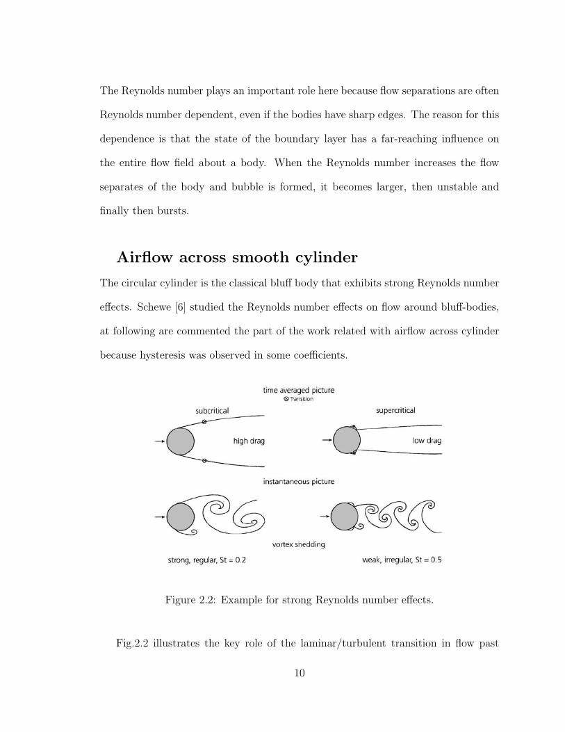
Airflow across smooth cylinder
The circular cylinder is the classical bluff body that exhibits strong Reynolds number
effects. Schewe [6] studied the Reynolds number effects on flow around bluff-bodies,
at following are commented the part of the work related with airflow across cylinder
because hysteresis was observed in some coefficients.
Figure 2.2: Example for strong Reynolds number effects.
Fig.2.2 illustrates the key role of the laminar/turbulent transition in flow past
10
a circular cylinder, both below and above the critical flow regime. The Reynolds
number effects here are clearly evident and dramatic. These phenomena, which are
triggered by the transition from laminar to turbulent flow, have characteristics that
are universally valid because they occur in similar form in flow over bodies having
other cross-sections.
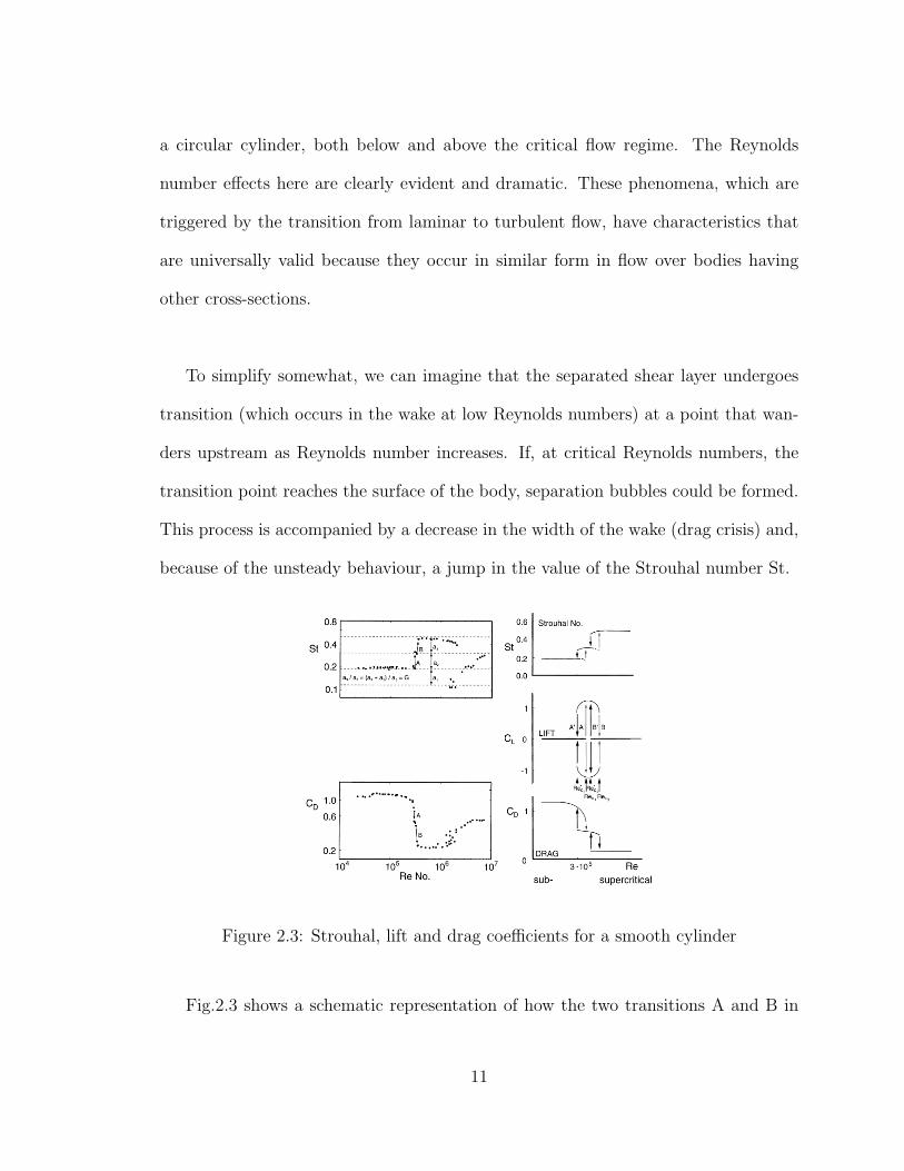
To simplify somewhat, we can imagine that the separated shear layer undergoes
transition (which occurs in the wake at low Reynolds numbers) at a point that wan-
ders upstream as Reynolds number increases. If, at critical Reynolds numbers, the
transition point reaches the surface of the body, separation bubbles could be formed.
This process is accompanied by a decrease in the width of the wake (drag crisis) and,
because of the unsteady behaviour, a jump in the value of the Strouhal number St.
Figure 2.3: Strouhal, lift and drag coefficients for a smooth cylinder
Fig.2.3 shows a schematic representation of how the two transitions A and B in
11

the critical flow region are mirrored by the characteristic coefficients CD; CL; and
St. With reference to the lift, the two transitions can be interpreted as subcritical
bifurcations at two critical Reynolds numbers. Both transitions are distinguished by
a discontinuous decline of drag, a jump in the value of the Strouhal number, and
hysteresis effects.
Von Karman Vortex Street
A vortex street will only be observed over a given range of Reynolds numbers, typ-
ically above a limiting Reynolds number value of about 90. The range of Reynolds
number values will vary with the size and shape of the body from which the eddies
are being shed, as well as with the kinematic viscosity of the fluid.
A particular vortex street situation was studied by Von Karman. It is a repeating
pattern of swirling vortices caused by the unsteady separation of flow over bluff bod-
ies. This case illustrates Strouhal instability and the particular wake known as Von
Karman Vortex Street. It is a succession of vortices created close to the cylinder
that break away alternatively from both sides of the cylinder. Vortices are emitted
regularly and rotate in opposite senses.
Figure 2.4: Example of Von Karman vortex street.
12
2.2.3 Static Stall of an Airfoil [4]
This phenomenon is not very well understood. It happens in particular positions of
an airfoil when a airflow goes around on it. It is caused by massive flow separation
resulting in sharp drop in lift and increase in the drag acting on the airfoil. The
prediction of the hysteresis associated at this phenomenon was studied by S. Mittal
and P. Saxena. They made an effort to study the behavior of the flow near stall, over
the body NACA 0012 airfoil, by solving the governing equations numerically. The
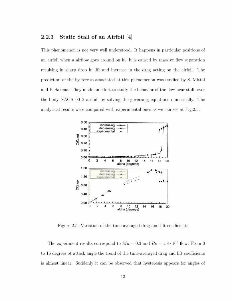
analytical results were compared with experimental ones as we can see at Fig.2.5.
Figure 2.5: Variation of the time-averaged drag and lift coefficients
The experiment results correspond to Ma = 0.3 and Re = 1.8 · 106 flow. From 0
to 16 degrees ot attack angle the trend of the time-averaged drag and lift coefficients
is almost linear. Suddenly it can be observed that hysteresis appears for angles of
13

attack close to the stall angle. The computations indicated that the flow ceases to be
steady beyond α = 17 deg and vortex shedding was observed at Fig.2.6.
Figure 2.6: Vorticity and pressure fields for the computed solutions
Their arguments about how to explain the hysteresis behavior appeared were that
the flow has the ability to remember its past history. For the same angle of attack, the
flow obtained with the increasing angle results in an almost attached flow with higher
lift and lower drag, whereas the one with decreasing angle of attack is associated with
large unsteadiness, lower lift, and higher drag.
14
Chapter 3
Geometry of the Probes
Multi-hole probes are commercially available in several configurations. These can be
classified in two main groups: by geometry shape or by the number of sensing holes.
However, the combination of both permits find probes of a concrete geometry with
3, 5 or 7 holes.
The most common shapes for probes head geometries are: cobra head, trapezoidal
head and cylindrical. Prismatic and cone forms are used as well, but due to their
less streamlined shape the calibration has to be done completely empirical. The most
well known and widely used are the three-hole pressure probes, as the name indicate
are characterized by three pressure sensing holes lying in one plane, which ones are
used in the present work.
These have mainly three different types of head geometries: cobra, trapezoidal
and cylinder head. The head shape and hole arrangements are plotted in Fig.3.1
where the yaw angle is also identified.
The probes when are introduced in a flow field create a flow disturbance due to is
15
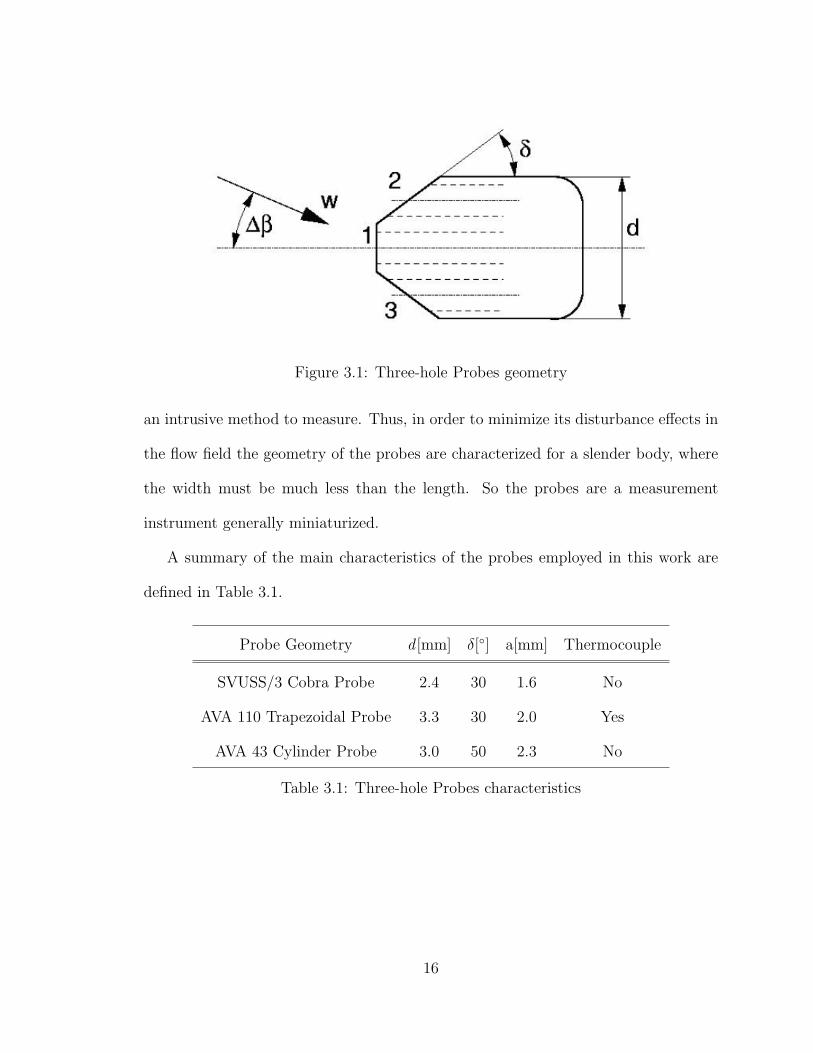
Figure 3.1: Three-hole Probes geometry
an intrusive method to measure. Thus, in order to minimize its disturbance effects in
the flow field the geometry of the probes are characterized for a slender body, where
the width must be much less than the length. So the probes are a measurement
instrument generally miniaturized.
A summary of the main characteristics of the probes employed in this work are
defined in Table 3.1.
Probe Geometry d [mm] δ[◦] a[mm] Thermocouple
SVUSS/3 Cobra Probe 2.4 30 1.6 No
AVA 110 Trapezoidal Probe 3.3 30 2.0 Yes
AVA 43 Cylinder Probe 3.0 50 2.3 No
Table 3.1: Three-hole Probes characteristics
16
3.1 SVUSS/3 Cobra Probe
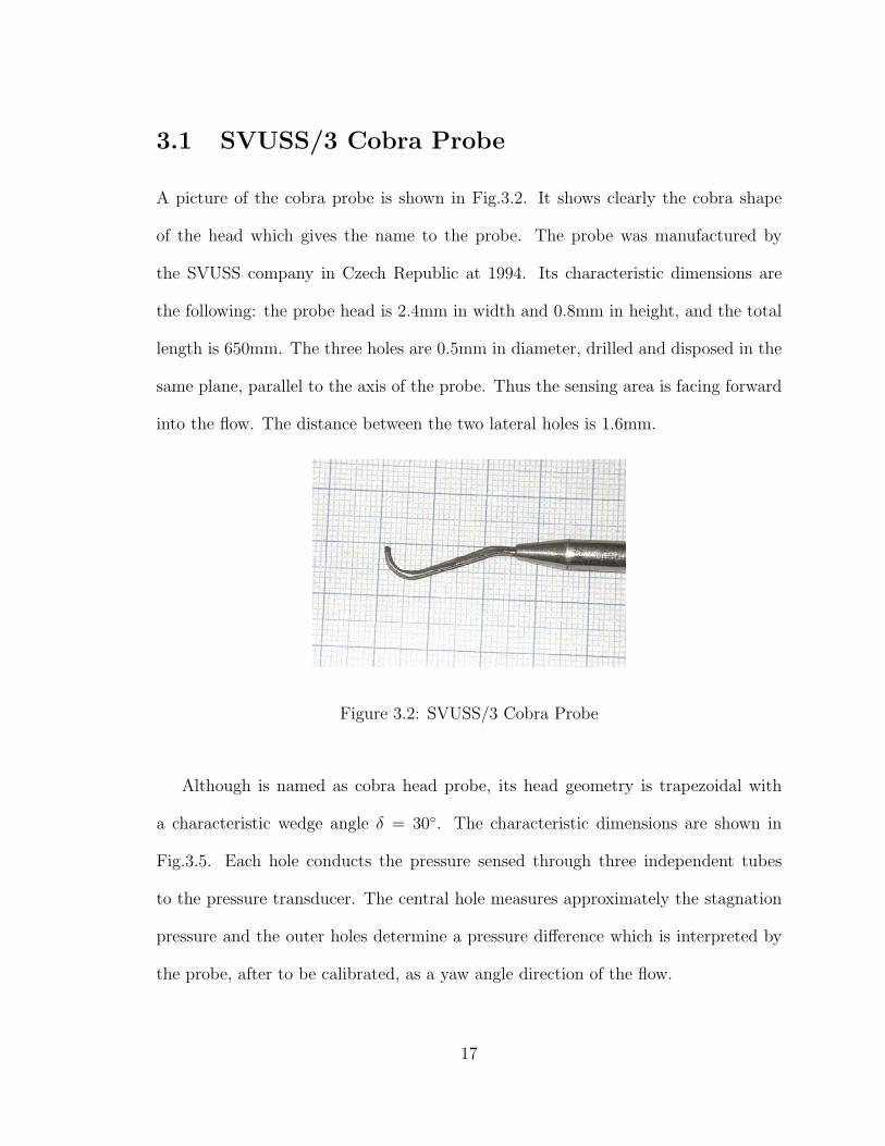
A picture of the cobra probe is shown in Fig.3.2. It shows clearly the cobra shape
of the head which gives the name to the probe. The probe was manufactured by
the SVUSS company in Czech Republic at 1994. Its characteristic dimensions are
the following: the probe head is 2.4mm in width and 0.8mm in height, and the total
length is 650mm. The three holes are 0.5mm in diameter, drilled and disposed in the
same plane, parallel to the axis of the probe. Thus the sensing area is facing forward
into the flow. The distance between the two lateral holes is 1.6mm.
Figure 3.2: SVUSS/3 Cobra Probe
Although is named as cobra head probe, its head geometry is trapezoidal with
a characteristic wedge angle δ = 30◦. The characteristic dimensions are shown in
Fig.3.5. Each hole conducts the pressure sensed through three independent tubes
to the pressure transducer. The central hole measures approximately the stagnation
pressure and the outer holes determine a pressure difference which is interpreted by
the probe, after to be calibrated, as a yaw angle direction of the flow.
17
3.2 AVA 110 Trapezoidal Probe
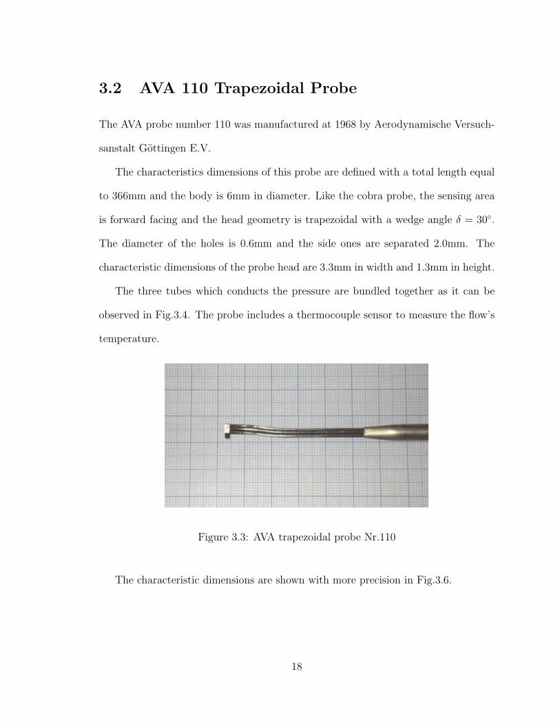
The AVA probe number 110 was manufactured at 1968 by Aerodynamische Versuch-
sanstalt Gottingen E.V.
The characteristics dimensions of this probe are defined with a total length equal
to 366mm and the body is 6mm in diameter. Like the cobra probe, the sensing area
is forward facing and the head geometry is trapezoidal with a wedge angle δ = 30◦.
The diameter of the holes is 0.6mm and the side ones are separated 2.0mm. The
characteristic dimensions of the probe head are 3.3mm in width and 1.3mm in height.
The three tubes which conducts the pressure are bundled together as it can be
observed in Fig.3.4. The probe includes a thermocouple sensor to measure the flow’s
temperature.
Figure 3.3: AVA trapezoidal probe Nr.110
The characteristic dimensions are shown with more precision in Fig.3.6.
18

3.3 AVA 43 Cylinder Probe
AVA cylinder probe number 43 was manufactured by Aerodynamische Versuchsanstalt
Gottingen E.V.
Figure 3.4: AVA 43 Cylinder Probe
As its name indicates, the head geometry of this probe is a cylinder of 3.00mm in
diameter, which is the characteristic dimension. The characteristic angle is δ = 50◦
and defines the position of the outer holes respect the perpendicular plane of the
probe axis.
The probe is shown in Fig.3.4. Its total length is 335mm and the diameter of the
main body is 6mm. The central hole number 1 is 0.3mm in diameter and the outer
holes are 0.6mm diameter, being the distance between these two holes of 2.3mm.
The characteristic dimensions are shown with more precision in Fig.3.7.
19
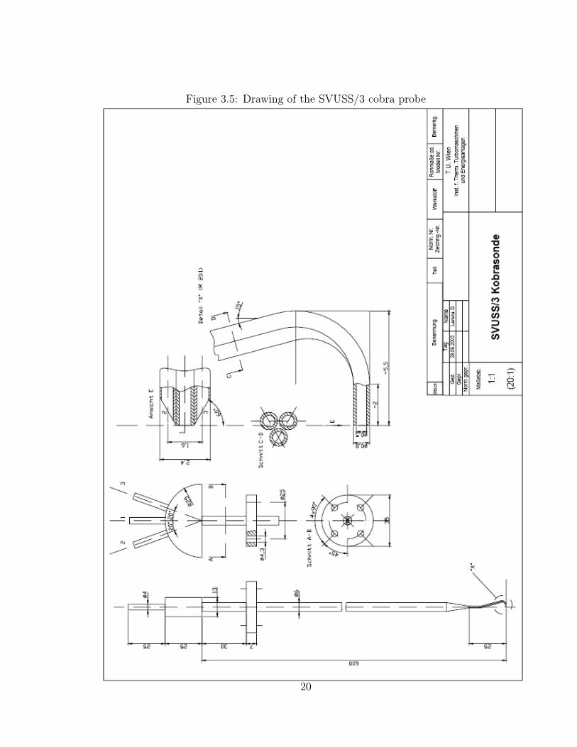
Figure 3.5: Drawing of the SVUSS/3 cobra probe
20

Figure 3.6: Drawing of the AVA 110 trapezoidal probe
21
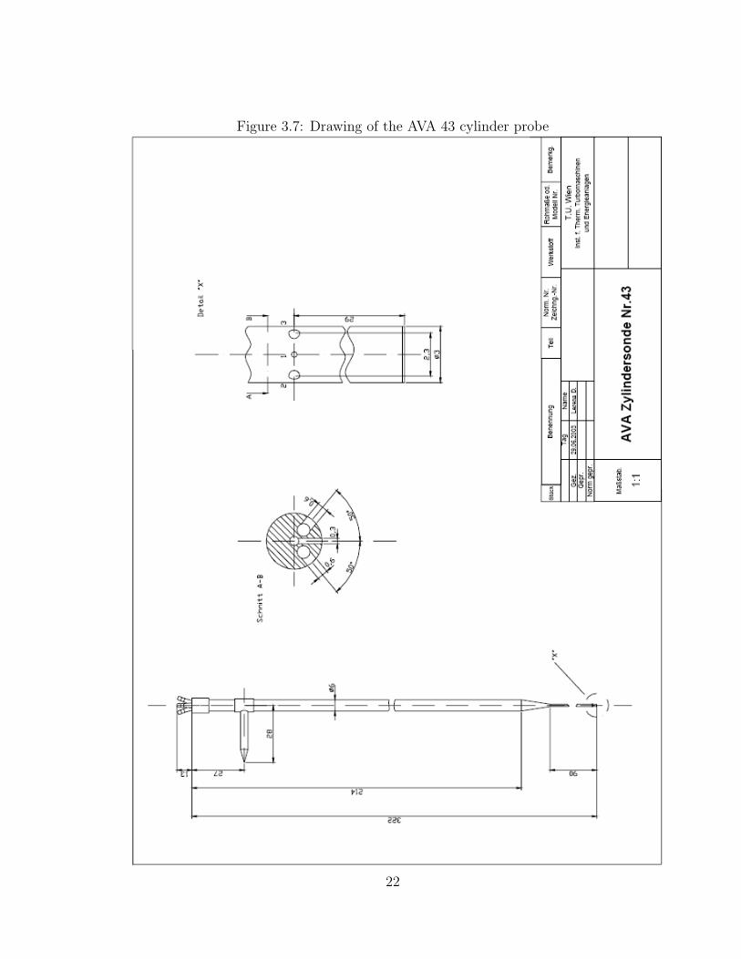
Figure 3.7: Drawing of the AVA 43 cylinder probe
22
Chapter 4
Experimental Calibration
4.1 About the Calibration
In many complex flow fields such as those encountered in turbomachines, the experi-
mental determination of the steady-state three-dimensional characteristics of the flow
field are frequently required. This application requires calibration data which are not
usually supplied by the manufacturer. Thus, the measurement of these data and the
development of an interpolation procedure become the responsibility of the user.
Due to nature of this work it is important to define the most important charac-
teristics of the measurement systems. Even though we can distinguish between two
main groups: static and dynamic characteristics, it is only considered the first one
because is more relevant for this experimental analysis. The static characteristics of
an instrument describe the behavior of variables that change very slowly. In these
cases, the instrument has time enough to reach the steady point before take the next
23
measure. The set: probe and piezoresisitve transducer, is the instrument of measure
used in this work. The following are the most important parameters to typify a in-
strument of measure.
Associated with range:
• Range: Interval of values of the measured variable among higher and lower limit
of the measure capacity of the measurement system.
• Span: Algebraic difference between the higher and lower value of the range.
• Dead zone: Zone where the input does not makes change the output measure-
ment value. So, does not produce reaction.
Associated with detail:
• Accuracy: Is the degree of conformity of a measured calculated quantity to its
actual (true) value.
• Precision: Is the degree to which further measurements or calculations show
the same or similar result. The results of calculations or a measurement can be
accurate but not precise; precise but not accurate; neither; or both. A result is
called valid if it is both accurate and precise.
• Sensitivity: Is the study of how output varies with changes in inputs. The
element of measure is said to be sensitive to an input if changing that input
variable changes the model output. This output variability (numerical or oth-
erwise) can be apportioned, qualitatively or quantitatively, to different sources
of variation in the inputs.
24

• Resolution: Is the level of detail that the measurement system is able to read.
Associated with reaction:
• Linearity: A measurement system is linear if the relation between the input
x and the output y follows the function y=k(x-x0) where k and x0 are con-
stants. As much linear would be the measurement system more easier will be
to calibrate it.
• Saturation: Zone where the measurement system has overtaken the maximum
operation range, thereby presents an unconfident behavior.
• Hysteresis: At a given input, the output is different if we reach it increasing
the input or decreasing it. We can’t predict the output without looking at
the history of the input. In order to predict the output, we must look at the
path that the input followed before it reached its current value. A system with
hysteresis has memory.
The fact that we want to study the effect of Reynolds number over the pressure co-
efficients and the possible hysteresis that could appears, obligate us to know which
is the hysteresis inherent at measurement system, if it exists, to correct the obtained
measurements.
4.1.1 Nulling technique
Probes can operate in two manners, in nulling or non-nulling technique. Nulling is a
technique where the probe is always perfectly oriented and aligned at the axis parallel
25

to the flow. In this position the central hole measure approximately the stagnation
pressure. In three-hole probes, the pressure sensed by the lateral holes theoretically
must be equal. But in fact, slight differences due to manufacturing imperfections or
variability of the flow field are usually observed. If the probe is measuring a two-
dimensional flow field and the pressure sensed by the lateral holes are meaningfully
different, it means that exist an angle among the X-axis of the probe and the velocity
vector, which is defined as a yaw angle.
Non-nulling technique, or also called stationary method, gives the solution at
this situation through the calibration curves yield by the experimental calibration.
This permits to find out the velocity vector of the flow field interpolating the mea-
sured pressures into the calibration curves. The main advantage of this method is
its simplicity which is very important in turbomachinery. On the other hand, nulling
technique provides a more accurate and precise measures but needs a device that
null the probe continuously. This device is governed by the pressure difference of the
outer holes, moving the probe in order to find a position where the pressure difference
become zero. Depending of the time of response of this device and the data acquisi-
tion system it can take long time to find out the nulling position, which makes this
technique not practical for applications with high variability of the flow field direction.
Calibrate the probes over a range of yaw angles is not the objective of this work.
Therefore, all the experiments are performed under nulling conditions.
26
4.1.2 Definition of the coefficients
The Navier-Stokes equations describe the motion of fluid substances such as liquids
and gases. They ara a set of differential and non linear ecuations that may be used
to model weather, ocean currents, water flow in a pipe, flow around an airfoil, and
motion of stars inside a galaxy, and in general, for any phenomenon with any kind of
fluid. These equations are obtained employing conservation of the mass and momen-
tum.
The vast majority of work on the Navier-Stokes equations is done under an incom-
pressible flow assumption for Newtonian fluids. The incompressible flow assumption
typically holds well even when dealing with a ”compressible” fluid, such as air at
room temperature (even when flowing up to about Mach 0.3). Taking the incompress-
ible flow assumption into account and assuming constant viscosity, the Navier-Stokes
equations will read (in vector form)
ρ
(∂w
∂t+ w · ∇w
)= −∇p+ µ∇2w + f (4.1)
A solution of the Navier-Stokes equations is called a velocity field or flow field,
which is a description of the velocity of the fluid at a given point in space and time.
Once the velocity field is solved for, other quantities of interest (such as flow rate,
drag force, or the path a ”particle” of fluid will take) may be found. There are ana-
lytic solutions only for very concrete situations. For the rest of situations, numerical
analysis is needed to solve the equations. The branch occupied to solve it is called
Computational Fluid Dynamics. The formulation employed in this work is so much
simple than the equation of Navier-Stokes, because we assume a set of simplifying
27
hypothesis which facilitates its solution. Actually the degree of precision needed for
this work does not make practical to use CFD.
Under the assumption that the flow field provided by the wind tunnel is an one-
dimensional steady flow. The turbulence is supposed very low, the characteristics of
the wind tunnel say that is approximately 1%, so it can be considered as negligible.
These simplifications drops out many terms of the Eq.(4.1). As a result, it is obtained
the Bernouilli conservation equation, which states that stagnation pressure is the sum
of static pressure and dynamic pressure,
p+1
2ρw2 = const (4.2)
The dynamic pressure is the second term of the above equation and represents
fluid kinetic energy. Static pressure p is not associated with the fluid motion but
rather with its state. The velocity is not a parameter which can be measured with a
probe, but it can be calculated from the measurements of the total and static pressure.
w =
√pt − pρ/2
(4.3)
Reynolds number is a non-dimensional parameter widely used in fluid motion. It
expresses relation between inertial and viscous forces of the flow, useful to identify
the flow regime.
Red =wd
ν(4.4)
The subscript d indicate that it is calculated with the characteristic diameter of the
probe, which is the probe width.
28
Mach number allows to assume that one gas at low velocity can be considered as
incompressible.
Ma =w
w0
(4.5)
Treaster and Yocum coefficients
The pressure sensed by the hole is measured as the moving air brought to rest. For
each hole the pressure can be expressed as a non-dimensional pressure coefficient as
the following formula.
ki =pi − pρ2w2
(4.6)
where i identify the hole of the probe.
The hole pressure coefficients are used to reduce the data on the non-dimensional
coefficients defined by Treaster and Yocum [8].
Direction coefficient,
kβ =p2 − p3
p1 − p=k2 − k3
k1 − k(4.7)
Total pressure coefficient,
kt =p1 − ptp1 − p
=k1 − 1
k1 − k(4.8)
Static pressure coefficient,
ks =p− pp1 − p
=k
k1 − k(4.9)
Dynamic pressure coefficient was not defined by Treaster and Yocum, it was
defined by the manufacturer of SVUSS/3 cobra probe. It is used in this work in order
29

to compare our results with the calibration data supplied by them.
kd =pt − pp1 − p2
=1
k1 − k2
(4.10)
where,
p =p2 + p3
2(4.11)
k =k2 + k3
2(4.12)
4.2 Streamline Projection Method
The streamline is a curve everywhere tangent to the instantaneous velocity vector of
the flow. It means that velocity vector has at each point the same direction as the
streamline. The streamline projection method is only valid under the hypothesis that
the free stream velocity is projected directly on each one of the three sensing holes,
with the assumption that the velocity magnitude is constant. In this situation the
holes are sensing the free stream static pressure in addition at the dynamic pressure
which velocity component is normal at them. This means that the holes of the
probe are measuring the total pressure as a sum of static and dynamic pressure. The
sreamline projection method can also be used for an approximation of the influence
of a velocity gradient [10] as well to find out the influence of a wall proximity effect
[9] which can be interpreted such a flow angle error. But these applications are not
the aim of this work.
The mathematical formulation is the following,
pi = p+1
2ρw2
i (4.13)
30

where the subscript i refers to the subject pressure. Employing the equations that
defines the hole calibration coefficients we obtain,
pi = p+ki2ρw2
i (4.14)
Then we can rewrite the hole coefficient as a combination of Eq.(4.13) and (4.14).
ki =(wiw
)2
(4.15)
All restrictions of this method above explained, makes that streamline projection
method could be considered as a purely geometrical method, due to the probe head
geometry is the only parameter dependant. But it is a quite good and easy way to
estimate the hole coefficients analytically.
The three probes used in this work, even though they have different head dimensions,
there are only two different shapes of the sensing forward area, trapezoidal and cylin-
der. Hence the streamline projection equations will be different not for each probe,
but rather for each shape of the head.
Next step is applying the streamline equations to deduce the pressure sensed by the
holes, decomposing the velocity vector in the normal direction at each hole of every
probe head geometry.
4.2.1 Trapezoidal head
As is it said before, SVUSS/3 cobra probe and AVA 110 trapezoidal probe have the
same characteristic wedge angle δ = 30◦, thus for this sort of head probe the stream-
line equations are valid for both.
31
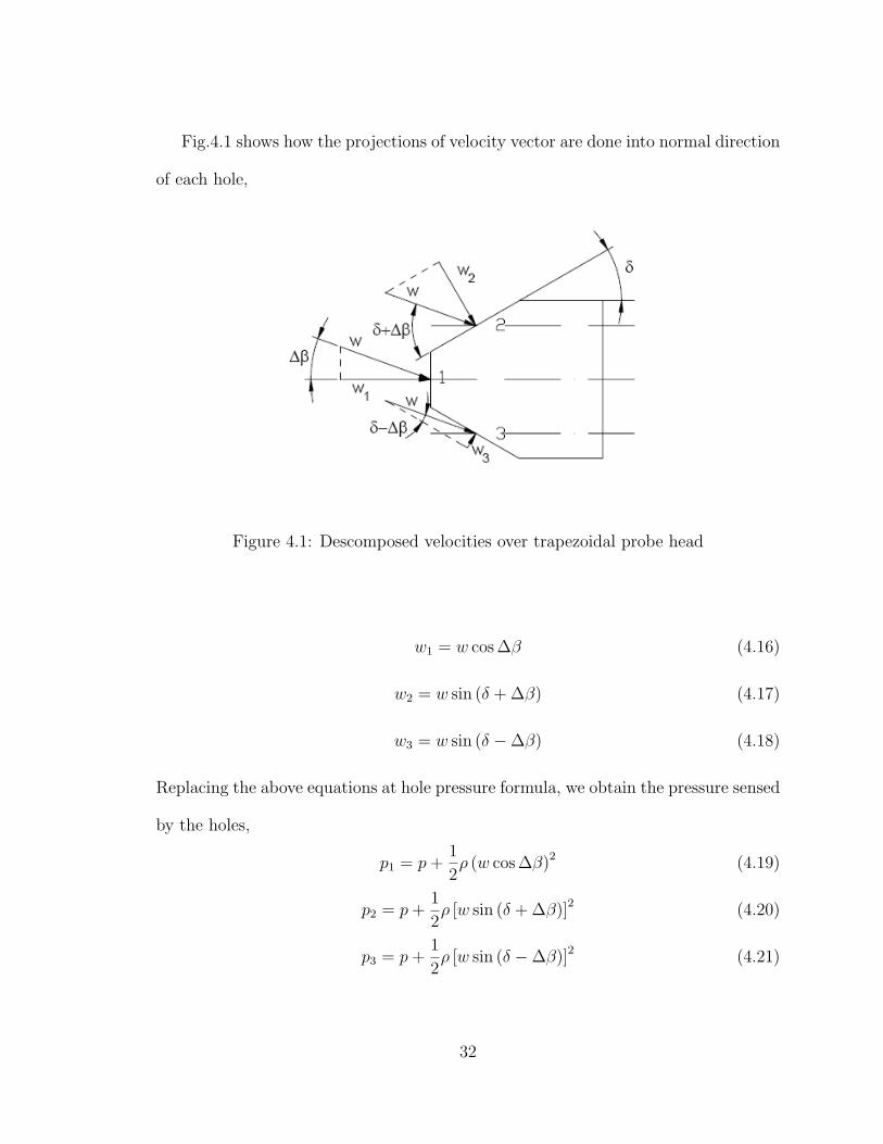
Fig.4.1 shows how the projections of velocity vector are done into normal direction
of each hole,
Figure 4.1: Descomposed velocities over trapezoidal probe head
w1 = w cos ∆β (4.16)
w2 = w sin (δ + ∆β) (4.17)
w3 = w sin (δ −∆β) (4.18)
Replacing the above equations at hole pressure formula, we obtain the pressure sensed
by the holes,
p1 = p+1
2ρ (w cos ∆β)2 (4.19)
p2 = p+1
2ρ [w sin (δ + ∆β)]2 (4.20)
p3 = p+1
2ρ [w sin (δ −∆β)]2 (4.21)
32
The hole coefficients are,
k1 = cos2 ∆β (4.22)
k2 = sin2 (δ + ∆β) (4.23)
k3 = sin2 (δ −∆β) (4.24)
As it is showed at the above equations, the holes coefficients are only dependent of
geometric parameters such as yaw angle as well as on the wedge angle of the probe’s
head. These also can be used to calculate the direction, total, static and dynamic
pressure coefficients at Eq.(4.7), Eq.(4.8), Eq.(4.9) and Eq.(7.1) respectively.
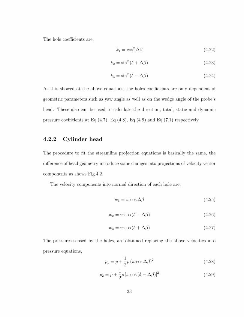
4.2.2 Cylinder head
The procedure to fit the streamline projection equations is basically the same, the
difference of head geometry introduce some changes into projections of velocity vector
components as shows Fig.4.2.
The velocity components into normal direction of each hole are,
w1 = w cos ∆β (4.25)
w2 = w cos (δ −∆β) (4.26)
w3 = w cos (δ + ∆β) (4.27)
The pressures sensed by the holes, are obtained replacing the above velocities into
pressure equations,
p1 = p+1
2ρ (w cos ∆β)2 (4.28)
p2 = p+1
2ρ [w cos (δ −∆β)]2 (4.29)
33
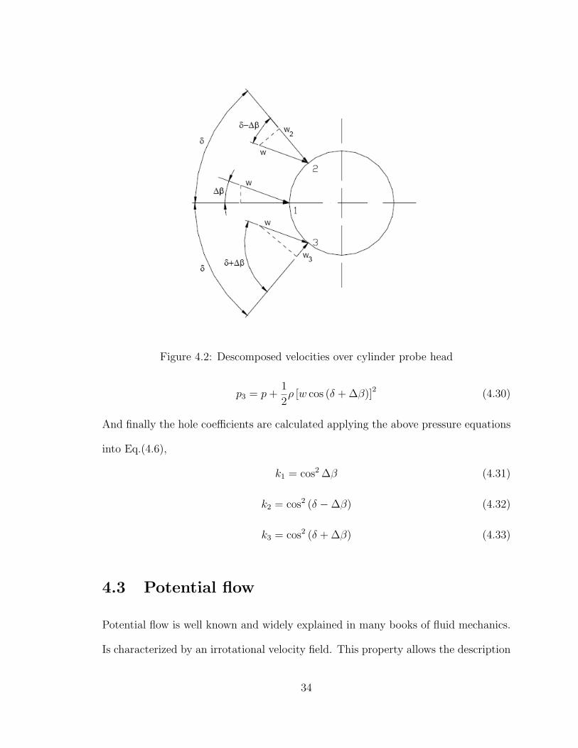
Figure 4.2: Descomposed velocities over cylinder probe head
p3 = p+1
2ρ [w cos (δ + ∆β)]2 (4.30)
And finally the hole coefficients are calculated applying the above pressure equations
into Eq.(4.6),
k1 = cos2 ∆β (4.31)
k2 = cos2 (δ −∆β) (4.32)
k3 = cos2 (δ + ∆β) (4.33)
4.3 Potential flow
Potential flow is well known and widely explained in many books of fluid mechanics.
Is characterized by an irrotational velocity field. This property allows the description
34

of the velocity field as the gradient of a scalar function as equation below also called
Laplace’s equation,
∇2Φ = 0 (4.34)
This equation can be used to calculate solutions to many practical flow situations.
Potential flow does not include all the characteristics of flows that are encountered in
the real world. For example, potential flow excludes turbulence, which is commonly
encountered in nature.
From potential flow are obtained lines of constant ψ that are known as streamlines
and lines of constant ϕ known as equipotential lines. Equipotentials are lines of equal
head that are in direct relation to pressure. Streamlines are perpendicular to the
equipotentials and have the same direction of the flow.
The result of applying this theory of potential flow around a cylinder is the below
equation,
ki =p(ϕ)− p
12ρw2
= 1− 4 sin2 ϕ (4.35)
where the angle ϕ is measured between flow direction and the cylinder radius that
goes across the hole i. Considering the geometry of the cylinder head probe, the
Eq.4.35 becomes the following expression for each hole.
k1 = 1− 4 sin2 ∆β (4.36)
k2 = 1− 4 sin2 (δ −∆β) (4.37)
k3 = 1− 4 sin2 (δ + ∆β) (4.38)
The hole coefficients of both methods can be also used to calculate the nondimen-
sional coefficients defined by Treaster and Yocum.
35
4.4 Calibration Procedure
The calibration procedure is the same for the three probes. The calibration is done
within a range of velocities between 19 up to 78m/s. Mach number is always lower
than 0.3 which allows assuming that the fluid is incompressible. Actually the highest
Mach numer reached is 0.23, so this assumption can be done without introduce error
at the measures.
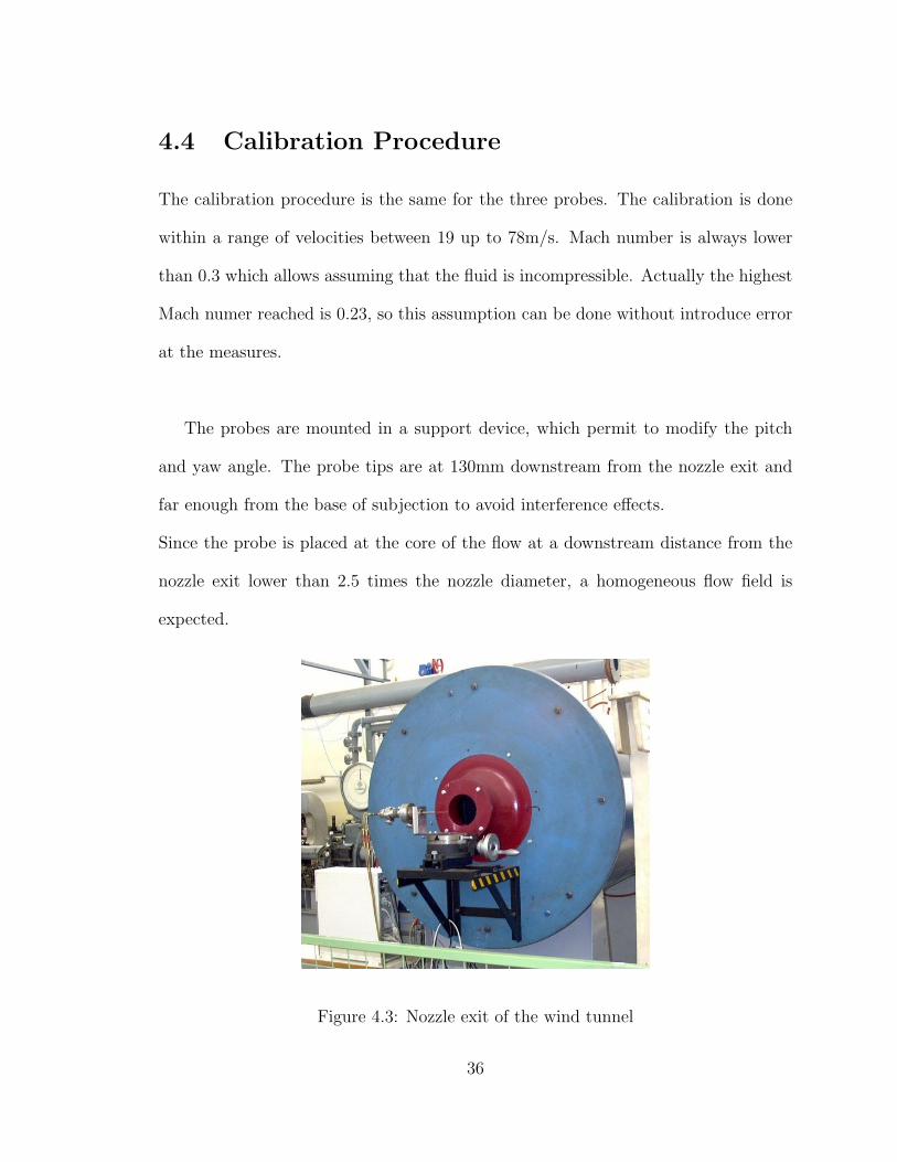
The probes are mounted in a support device, which permit to modify the pitch
and yaw angle. The probe tips are at 130mm downstream from the nozzle exit and
far enough from the base of subjection to avoid interference effects.
Since the probe is placed at the core of the flow at a downstream distance from the
nozzle exit lower than 2.5 times the nozzle diameter, a homogeneous flow field is
expected.
Figure 4.3: Nozzle exit of the wind tunnel
36
Before to start to perform the calibration, the probes were nulled manually. The
holes 2 and 3 were connected to a tube in U with water in its interior to measure the
differential pressure. The probe was placed at the support device and subjected to
an air flow supplied by the wind tunnel. It amended the angle yaw until the water
level of the two tubes was the same, which means that the pressure of the two side
holes is the same, therefore the probe is in nulling position.
Once the probes were nulled, the calibration starts setting the motor velocity at
400rpm. We take the measures and the next step is increase the motor velocity 50rpm.
The measures are taken again and the same procedure is done until reach 1600rpm.
Then it is followed the inverse sequence, the velocity of the motor is decreased in
steps of 50rpm until 600rpm taking measures at each step. The parameters measured
were the following:
• Flow temperature, T
• Hole pressures p1, p2, p3
• Total flow pressure pt
We take 30 single measures for each parameter during an interval of 0.2 seconds.
These measures are treated by LabVIEW, which through a data reduction program
calculates the mean of each parameter. Employing the measured data, the program
generates an output file with the following parameters, needed to evaluate and cali-
brate the probes:
• Flow velocity w
37

• Mach number Ma
• Reynolds number Red
• Hole coefficients ki
• Direction coefficient kβ
• Total pressure coefficient kt
• Static pressure coefficient ks
• Dynamic pressure coefficient kd
These parameters are calculated with the equations explained at the section 4.1.2,
called Definition of the coefficients.
38
Chapter 5
Test Facility
The experimental calibration of the three-hole probes has been carried out at the lab-
oratory of the Institute of Thermodynamics and Energy Conversion of the University
of Technology of Vienna.
The main equipment employed consists in a free jet wind tunnel, the three-hole
probes with different head geometries and the data acquisition system. The charac-
teristics of the probes were already described at Chapter 3.
The characteristics of the wind tunnel and the data acquisition system are de-
scribed below.
5.1 Wind Tunnel
A free jet wind tunnel is used for the probes calibration at different Reynolds numbers.
The velocity of the flow field is fixed manually using the transmission for speed control
which actuates on a 50kW DC motor. The motor drives a radial blower of 1115mm
in diameter, and it is able to supply 3m3/s airflow.
39

To avoid the high level of turbulence, the wind tunnel is equipped with nylon
screens placed upstream of the nozzle inlet. The objective is to obtain a homogenous
flow field downstream of the nozzle exit, thus it is possible to approximate that,
under nulling conditions, all holes are sensing the same X-axis velocity. The stream
wise turbulence intensity is about 1%. The throat diameter of the convergent nozzle
exit is 120mm and the probe head is mounted in a subjection structure at 130mm
downstream of the nozzle exit plane.
At the exit throat, there is a ring with 8 pressure sensors connected among them
to measure the total pressure at the exit of the wind tunnel. Also a Pt-100 resistor
thermometer, placed inside the wind tunnel, is used to measure the flow temperature.
The main technical characteristics of the free jet wind tunnel are summarized in
Table 5.1.
Characteristic Value
Power supply 50kW DC motor
Flow rate 3m3/s
Nozzle diameter 120mm
Contraction ratio 1:69.4
Diffuser divergence 5.7◦
Mach number 0.05 - 0.3
Reynolds number variable
Turbulence intensity ≈ 1%
Table 5.1: Technical data of the wind tunnel
40

Figure 5.1: Sketch of the wind tunnel
5.2 Data Acquisition System
The three-hole probes, as are defined at 3th chapter, are the medium for what the
sensed pressures at the head are driven through the tubes until the transducer. The
transducer is the element which measures quantitatively the pressure. Thus, is im-
portant to characterize the transducer.
The pressures are converted into electrical signals through a piezoresistive trans-
ducer. The operation system of a piezoresistive pressure transducer consist of flexible
diaphragms also called piezoelectric elements with a crystalline substance between
those that generates a voltage difference when is subject of mechanical deformations.
The piezoresistive pressure transducers is powered with 8V DC set manually with
an accuracy of ±1mV . Since the measured pressures are relative to the atmospheric,
these can be positive or negative. The piezoresistive transducer used is DA 27,
186PC03D. Fig.5.2 shows the behavior of the transducer.
A perfect linear relation over entire range is observed, which can be expressed
41

Figure 5.2: Transducer graph conversion
mathematically as the next formula. The units are [mbar] and [V], therefore the
conversion from pressure to voltage is immediate.
E = 0.014∆p+ 3.502 (5.1)
42
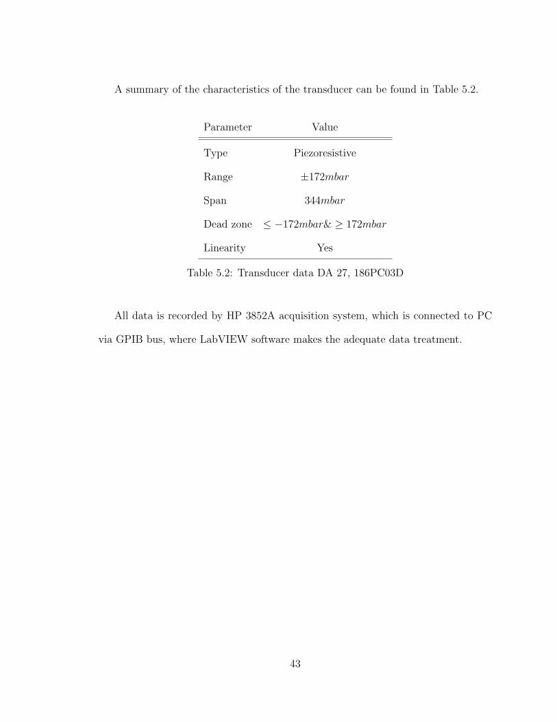
A summary of the characteristics of the transducer can be found in Table 5.2.
Parameter Value
Type Piezoresistive
Range ±172mbar
Span 344mbar
Dead zone ≤ −172mbar& ≥ 172mbar
Linearity Yes
Table 5.2: Transducer data DA 27, 186PC03D
All data is recorded by HP 3852A acquisition system, which is connected to PC
via GPIB bus, where LabVIEW software makes the adequate data treatment.
43
Chapter 6
Results and Discussion
In this chapter are evaluated the results obtained by the experiment made at the
facilities, following the procedure described at the Chapter 4. A complete set of data
is obtained for each probe. In order to make easier compare the results and the
behavior of the probes with the same head geometry, trapezoidal head, it is used the
same scale to plot the same coefficients. Adapting the scale at the values for each
coefficient but being the same for both probes.
The comments of the plots are also evaluated into a sorted and sequential form.
Presenting and analyzing firstly the hole coefficients, and afterwards the direction,
the total pressure, the static and the dynamic pressure coefficients, in this order. Fol-
lowing the aim of this work, the coefficients are plotted versus the Reynolds number.
A special emphasis is done into the analysis of the differences that could appear be-
tween the measures obtained while the velocity of the flow field increase respect the
obtained ones while the velocity decrease.
The coefficients calculated for each probe are also compared with the values cal-
44

culated with streamline projection method. In the case of the AVA 43 cylinder probe
the potential flow solution has been also studied. Both methods have been explained
previously at Chapter 4. The values that these methods provide are showed at the
Table 6.1.
Trapezoidal head Cylinder head
Coefficient Streamline[-] Streamline[-] Potential flow[-]
k1 1 1 1
k2 0.25 0.413 -1.347
k3 0.25 0.413 -1.347
kβ 0 0 0
kt 0 0 0
ks 0.333 0.704 -0.574
kd 1.333 1.704 0.426
Table 6.1: Coefficients calculated analytically
45
6.1 SVUSS/3 Cobra Probe
The environment conditions under which the experiment was developed are the fol-
lows:
• T = 16.5◦C, being 21.0◦C the maximum temperature reached.
• pa = 1002.6mbar of atmospheric pressure.
• Probe placed at the core of the flow field, 130mm downstream of the nozzle exit
and nulled manually. However the indicator marks −1.5◦ of yaw angle.
• Probe diameter = 2.4mm.
• Range of Reynolds number = 3000 up to 12000.
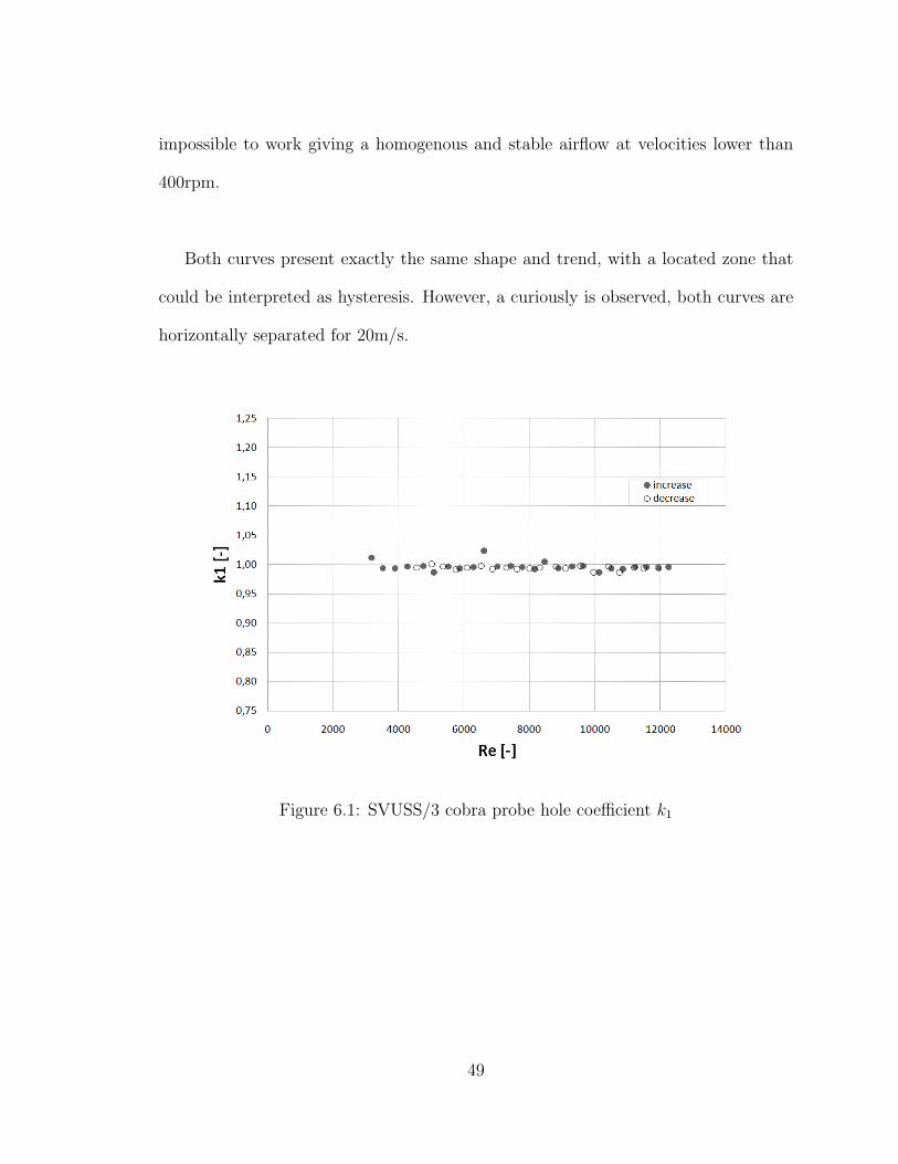
As it was expected, the value of k1 does not show any type of variation in relation
over the entire Reynolds number. It keeps constant in all the range. Due to for its
own definition in Eq.(4.22) the numerator and the denominator rise insofar that the
velocity of the flow field as well it does. The graph shows perfect consonance with
the value calculated using streamline projection method k1 = 1. Differences between
increasing and decreasing the flow velocity are not appreciated.
The coefficients of the two lateral holes of SVUSS/3 probe present a similar be-
havior. Both show a progressive decreasing trend at relatively low Reynolds numbers
until stabilizes between 7000 and 8000. From there, the value of the coefficients is
maintained more or less constant. This value approaches with quite good precision
at the value calculated by streamline projection method where k2 = k3 = 0.25 .
46

However, the trend showed by k3 is much clear than the trend of k2 which has more
dispersion and some values are very far of the trend line. The region with highest
degree of scatter is among 8000 and 10000 Reynolds number.
Naturally the direction coefficient in nulled position must be zero, as it is calcu-
lated through streamline projection method kβ = 0. Even though kβ is calculated
with the mean of k2 and k3, the error that introduce the deviation of the hole coeffi-
cient k2 respect the main trend generates a slight deviation of the direction coefficient
at low Reynolds numbers observed at the graph.
Total pressure coefficient presents almost the same comportment as the hole co-
efficient number one k1. Due to the probe is nulled k1 senses the stagnation pressure.
Although both plots are very similar, the most significant difference is the value being
kt = 0 instead of 1, in concordance with the streamline projection method.
Static pressure coefficient is the parameter that presents a more clear variation
with Reynolds number. The trend is basically the average of the values of the outer
holes coefficients as its formula implies. A deviation of the expected trend is observed
on the Reynolds number among 7000 and 9000, which modifies the normal trend
drawing a strange hill to finally reach the expected trend again. These anomalies are
observed for the increasing and also for the decreasing of the Reynolds number. Is
the only paramether that shows a possible hysteresis behavior.
47
Under nulled position, which means that k1 ≈ 1 and for its own definition makes
that the dynamic pressure coefficient is dependent only of k2. This fact explain why
the plot of kd is pretty like as the plot of k2, with the same degree and location of the
scatter.
An additional graph of dynamic pressure coefficient is included in order to com-
pare the experimental results and the calibration data provided by the manufacturer.
One realizes that the behavior shown by ks is very similar at that kd of the manufac-
turer shows. If both coefficients are analyzed numerically employing the streamline
projection equations, taking into consideration that the experiment is under nulling
conditions and ∆β = 0, it is easy to find the relation between them,
ks = tan2δ =sin2δ
cos2δ=
1− cos2δ
cos2δ(6.1)
And the value of kd for streamline projection method is,
kd =1
cos2δ(6.2)
Thus, if we combine the above equations we find,
kd = 1 + ks (6.3)
Thus, due to the great dispersion shown by kd. To contrast the results with greater
clarity, it considers appropriate to present in the same graphic kd (manuf.) and ks+1
(exp.). As it can be observed, the calibration data of the manufacturer cover a larger
range of Reynolds number than the obtained carrying out the experiment. This fact
is due to the technical limitations of the speed-control system of the motor that made
48
impossible to work giving a homogenous and stable airflow at velocities lower than
400rpm.
Both curves present exactly the same shape and trend, with a located zone that
could be interpreted as hysteresis. However, a curiously is observed, both curves are
horizontally separated for 20m/s.
Figure 6.1: SVUSS/3 cobra probe hole coefficient k1
49
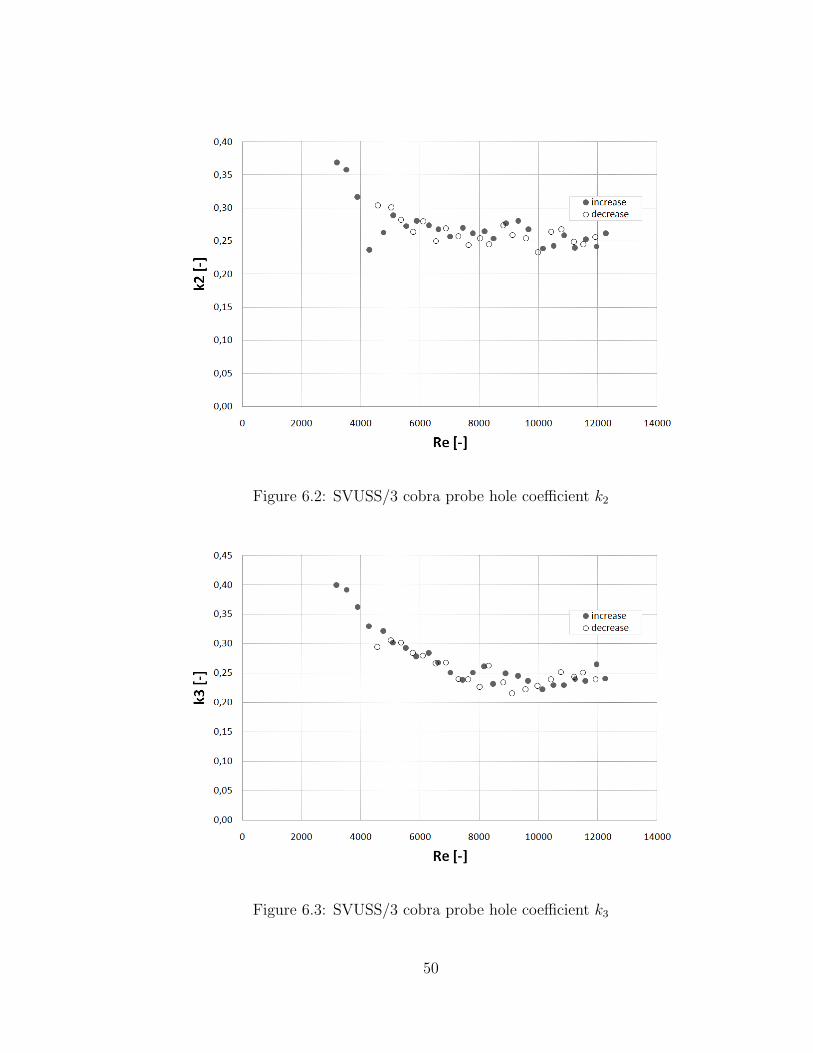
Figure 6.2: SVUSS/3 cobra probe hole coefficient k2
Figure 6.3: SVUSS/3 cobra probe hole coefficient k3
50

Figure 6.4: SVUSS/3 cobra probe direction coefficient kβ
Figure 6.5: SVUSS/3 cobra probe total pressure coefficient kt
51
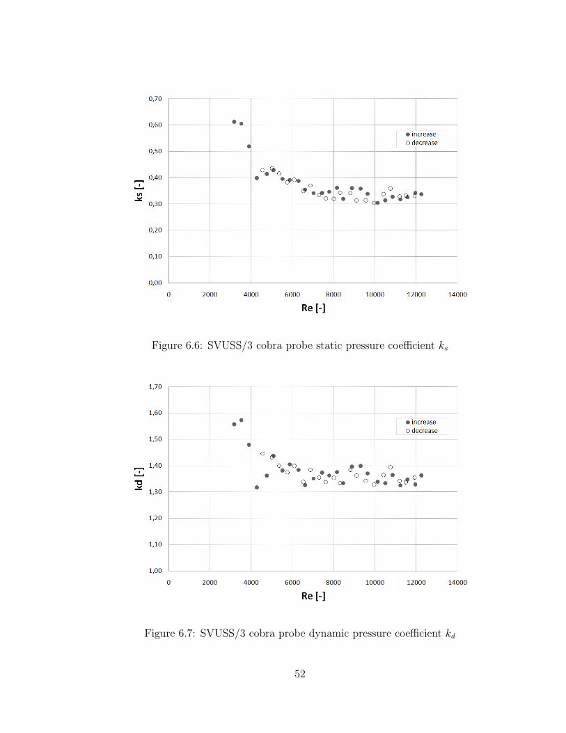
Figure 6.6: SVUSS/3 cobra probe static pressure coefficient ks
Figure 6.7: SVUSS/3 cobra probe dynamic pressure coefficient kd
52

Figure 6.8: Adapted kd as ks + 1 in comparison with kd of manufacturer data
6.2 AVA 110 trapezoidal probe
The environment conditions under which the experiment was developed are the fol-
lows:
• T = 17.3◦C, being 22.1◦C the maximum temperature reached.
• pa = 1002.4mbar of atmospheric pressure.
• Probe placed at the core of the flow field, at 130mm downstream of the nozzle
exit and nulled manually. However, the indicator marks −2.5◦ of yaw angle.
• Probe diameter = 3.3mm.
• Range of Reynolds number = 4500 up to 17500.
53
It is easily imaginable that two probes with the same head geometry, under the
same work conditions, will present similar behavior. As it is mentioned at the chapter
where the geometries of the probes are described, SVUSS/3 and AVA 110 have the
same trapezoidal head geometry with the same characteristic wedge angle. This fact
allows compare the results of both probes, and in function of those choose the proper
probe for a concrete application. The most meaningful difference between the plots of
the two probes is not the slope or the trend of the curves, because as it can be checked
are pretty much the same at the shown by SVUSS/3, it is the lateral movement in
the values for the X-axis for the Reynolds number. This fact is due to, even though
the velocities range that are the probe exposed is the same, the Reynolds number is a
non-dimensional parameter calculated with the characteristic diameter of the probe,
Eq.(4.4). As the characteristic diameter of the AVA 110 trapezoidal probe is 3.3mm
instead of 2.4mm of the SVUSS/3 cobra probe, it generates this lateral displacement
of 2000 units approximately. Being now the range of Reynolds number between 4000
and 17000. This difference was not observed if the graphics were submitted as the
evolution of any coefficient versus the velocity of the flow expressed in meters per
second. Due to the velocities range for all the probes of this work are approximately
between 20 and 80m/s.
The interpretation of the hole coefficients is basically the same as for SVUSS/3
cobra probe ones. k1 is completely plane in 1, only several points are far away from
the expected value. The other hole coefficiens k2 and k3, present a similar behavior.
The curve has a decreasing slope at low Reynolds number until it stabilizes at 10000.
From there, the degree of scatter increase, showing a high fluctuation of the values
54

until the end of the range. The average of all these points seems to be an horizon-
tal line of value a bit higher than 0.2, but far from the calculated with streamline
projection method that must be k2 = k3 = 0.25. Any of the hole coefficients show
significant differences between increasing and decreasing the Reynolds number.
Direction pressure coefficient presents a moderate degree of dispersion of the mea-
sures around the value predicted by streamline projection method where kβ = 0.
The argument that explains this scatter is the same that has been described for the
SVUSS/3 cobra probe, if kβ is calculated with k2 and k3 and these show dispersion,
it is logical that the direction coefficient has got it as well.
Total pressure coefficient does not show nothing special, very plane around zero.
Which means that the probe is quite well nulled. But if it is looked more attentively,
one can realize that most of the measures are slightly under zero. To that p1 − pt
would be negative, pt must be bigger than p1. Which means that there are a pressure
loss from where the total pressure is measured until where the probe is placed to
measure the total pressure through the hole number 1. This explanation is useful for
all the probes, as it can be checked at all the kt graphs.
Static pressure coefficient presents the same behavior than the outer hole coeffi-
cients. As it can be observed the slope of the curve follows the same trend but with
the singularity that the scatter has been reduced thanks that ks is calculated with
the average of the holes 2 and 3.
There is no significant differences on the measures of ks between increasing and de-
55
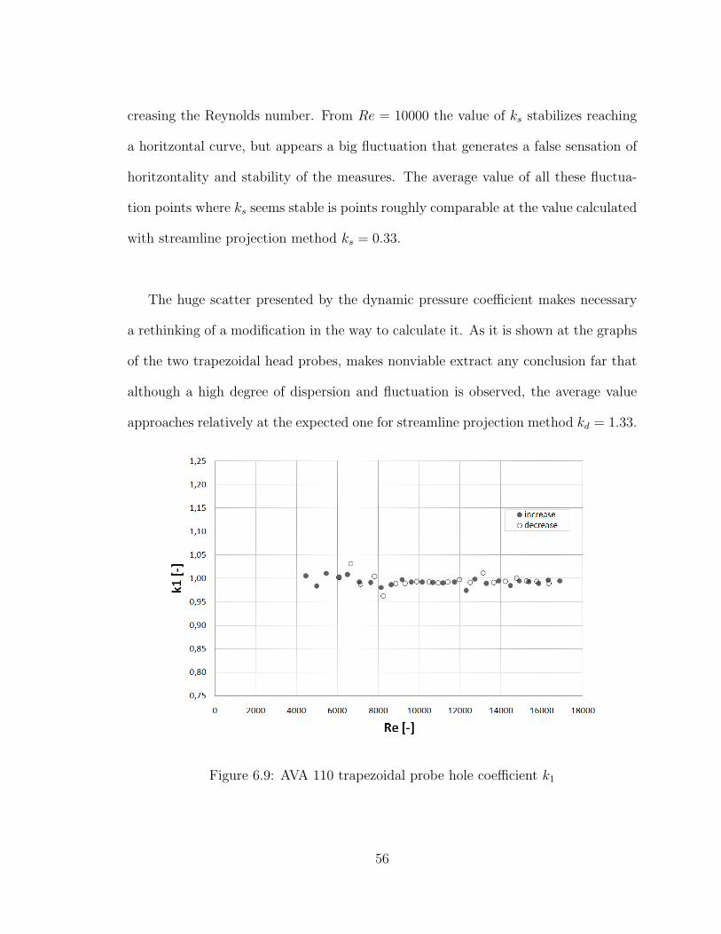
creasing the Reynolds number. From Re = 10000 the value of ks stabilizes reaching
a horitzontal curve, but appears a big fluctuation that generates a false sensation of
horitzontality and stability of the measures. The average value of all these fluctua-
tion points where ks seems stable is points roughly comparable at the value calculated
with streamline projection method ks = 0.33.
The huge scatter presented by the dynamic pressure coefficient makes necessary
a rethinking of a modification in the way to calculate it. As it is shown at the graphs
of the two trapezoidal head probes, makes nonviable extract any conclusion far that
although a high degree of dispersion and fluctuation is observed, the average value
approaches relatively at the expected one for streamline projection method kd = 1.33.
Figure 6.9: AVA 110 trapezoidal probe hole coefficient k1
56
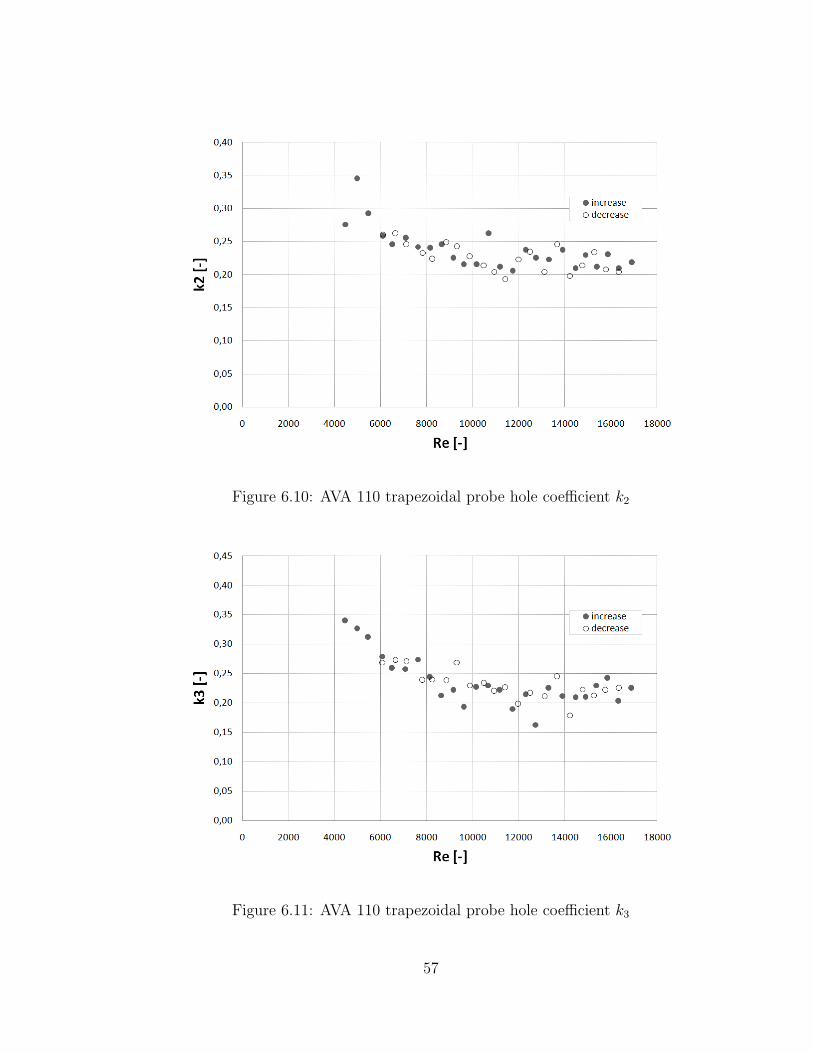
Figure 6.10: AVA 110 trapezoidal probe hole coefficient k2
Figure 6.11: AVA 110 trapezoidal probe hole coefficient k3
57

Figure 6.12: AVA 110 trapezoidal probe direction coefficient kβ
Figure 6.13: AVA 110 trapezoidal probe total pressure coefficient kt
58
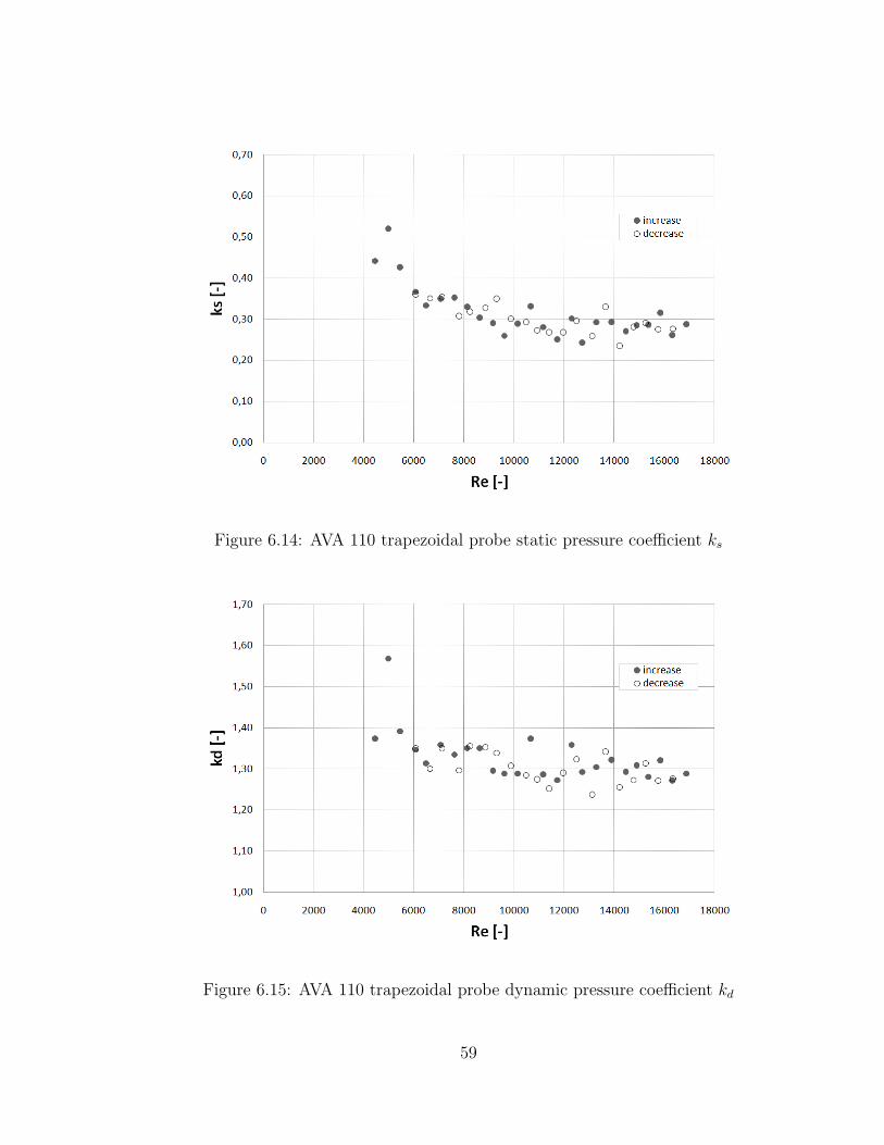
Figure 6.14: AVA 110 trapezoidal probe static pressure coefficient ks
Figure 6.15: AVA 110 trapezoidal probe dynamic pressure coefficient kd
59
6.3 AVA 43 cylinder probe
The environment conditions under which the experiment was developed are the fol-
lows:
• T = 17.4◦C, being 21.3◦C the maximum temperature reached.
• Pa = 1002.5mbar of atmospheric pressure.
• Probe placed at the core of the flow field, at 130mm downstream of the nozzle
exit and nulled manually.
• Probe diameter = 3.0mm.
• Range of Reynolds number = 4000 up to 16000.
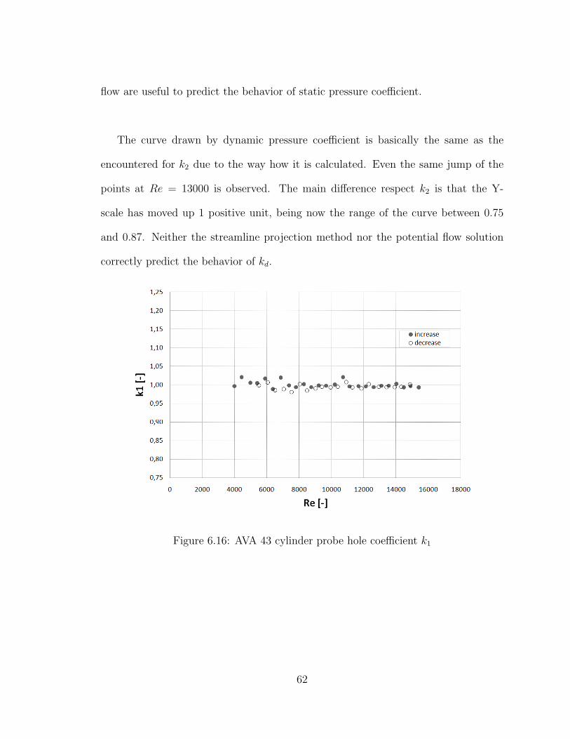
Hole coefficient k1 does not show any deviation respect the expected behavior, all
the measures are very close to k1 = 1 with independence if the velocity increases or
decreases. Some few points at low Reynolds number are a bit far from the mean,
but without meaningful importance. So, for k1 streamline projection method and
potential flow solutions yield the real value.
The coefficient k2 does not show the same comportment than k3, although the
probe is symmetric respect the X-axis parallel at the flow direction. The measures
draw a decreasing curve, but with a slope smaller than what k3 shows. At Re = 13000
the curve makes a strange jump of 0.5 units leaving far away the previous trend, fin-
ishing the sequence at −0.32. Almost 0.1 units of difference of the expected value, in
comparison with k3.
60
Huge differences are observed among the outer hole coefficients k2 and k3. The
coefficient k3 presents a curve with a very clear and progressive decreasing slope with
a degree of dispersion almost negligible, between the values −0.1 and −0.4. From
Re = 12000 the curve becomes a horizontal line that approach at −0.41.
The big diameter of the lateral holes could explain these differences respect the num-
bers calculated with streamline projection method or with potential flow, because the
holes can be sensig a share of the total pressure.
Direction coefficient displays a significant deviation respect the expected value
kβ = 0. This fact is due to the error introduced by the hole coefficient k2, that as has
been mentioned above, presents a huge difference respect the comportment shown by
the other hole coefficient k3.
Total pressure coefficient presents a very plane comportment like k1 does. With
independence of the Reynolds number, all points are very close to zero, which is in
agreement with the streamline projection method as well as with potential flow solu-
tion.
Static pressure coefficient shows how the fact to use the average of the outer holes
helps significantly to reduce the scatter. Unlike of kβ that is calculated as the rest
of k2 and k3, ks uses the mean. Thus if the trend of the static pressure coefficient is
clear, is thanks basically at the good behavior presented by k3. Streamline projection
method says that the value that would approach the curve must be 0.704, and from
potential flow must -0.574. The gap between them is very important and any of them
is close at the real value, ks = −0.25 . So streamline projection and neither potential
61
flow are useful to predict the behavior of static pressure coefficient.
The curve drawn by dynamic pressure coefficient is basically the same as the
encountered for k2 due to the way how it is calculated. Even the same jump of the
points at Re = 13000 is observed. The main difference respect k2 is that the Y-
scale has moved up 1 positive unit, being now the range of the curve between 0.75
and 0.87. Neither the streamline projection method nor the potential flow solution
correctly predict the behavior of kd.
Figure 6.16: AVA 43 cylinder probe hole coefficient k1
62
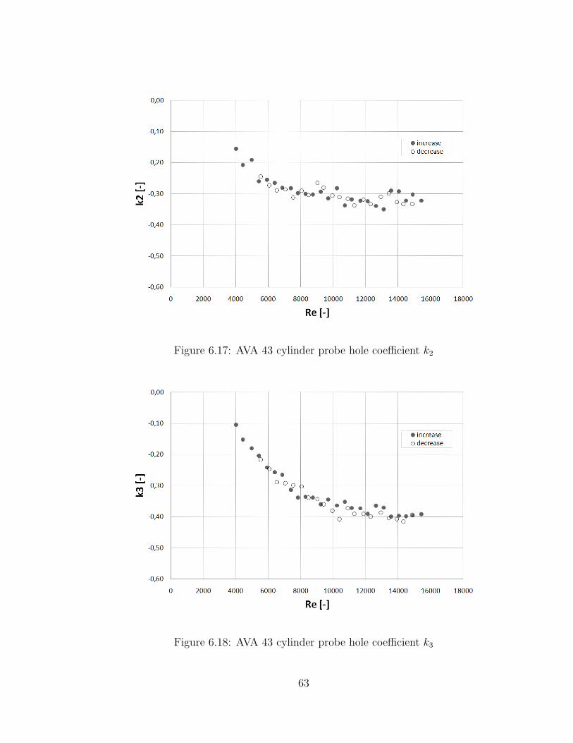
Figure 6.17: AVA 43 cylinder probe hole coefficient k2
Figure 6.18: AVA 43 cylinder probe hole coefficient k3
63

Figure 6.19: AVA 43 cylinder probe direction coefficient kβ
Figure 6.20: AVA 43 cylinder probe total pressure coefficient kt
64

Figure 6.21: AVA 43 cylinder probe static pressure coefficient ks
Figure 6.22: AVA 43 cylinder probe dynamic pressure coefficient kd
65
Chapter 7
Conclusions
All the coefficients except k1, kt and kβ show variation respect Reynolds number.
As it is mentioned at the previous chapter, under nulling conditions k1 and kt are
equivalents because they measure the same magnitude, the stagnation pressure. They
show a behavior completely plane with independence of the velocity of flow, either
increasing or decreasing the velocity. The direction coefficient kβ is not so useful
due to the experiment has carried out under nulling conditions, so its value must be
always zero, over the entire Reynolds range.
For the rest of coefficients, in all of them are notes a peculiarity in common. At
low airflow velocities they present, with greater or lesser degree and clarity, curves
with a descendant inclination that stabilizes from a certain speed, from that point
remains more or less constant until the end of range.
For a curve that draws the result of a division display an inclination, either posi-
66
tive or negative, means that the numerator not to vary in the same gives that makes
the denominator. While that when a curve shows a plane behavior is because the
variation of the numerator and denominator is constant.
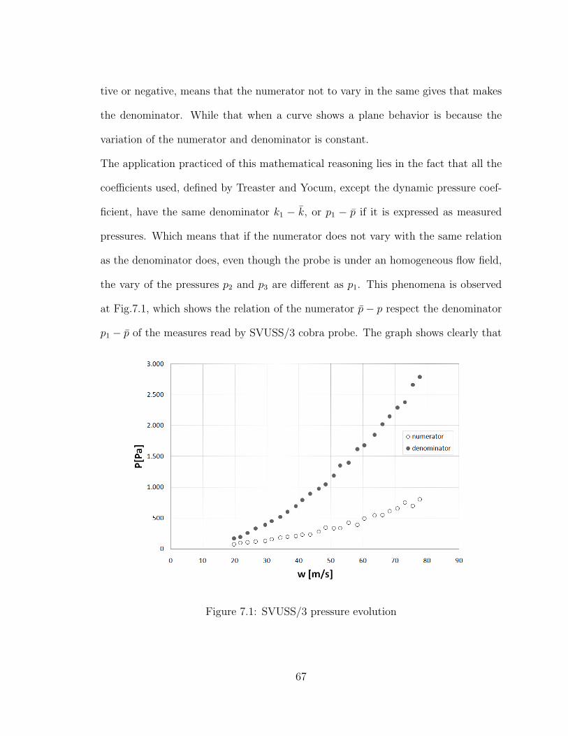
The application practiced of this mathematical reasoning lies in the fact that all the
coefficients used, defined by Treaster and Yocum, except the dynamic pressure coef-
ficient, have the same denominator k1 − k, or p1 − p if it is expressed as measured
pressures. Which means that if the numerator does not vary with the same relation
as the denominator does, even though the probe is under an homogeneous flow field,
the vary of the pressures p2 and p3 are different as p1. This phenomena is observed
at Fig.7.1, which shows the relation of the numerator p− p respect the denominator
p1 − p of the measures read by SVUSS/3 cobra probe. The graph shows clearly that
Figure 7.1: SVUSS/3 pressure evolution
67
p1− p presents a curve with a rising inclination, while the inclination of p−p remains
more or less constant.
The results have shown quite good agree between the values calculated with
streamline projection method and the values the curves approach when got stabi-
lized as horizontal line. As it is a merely geometric method, the values that provides
are constant. But if the process is inverted, from the measures it is possible to extract
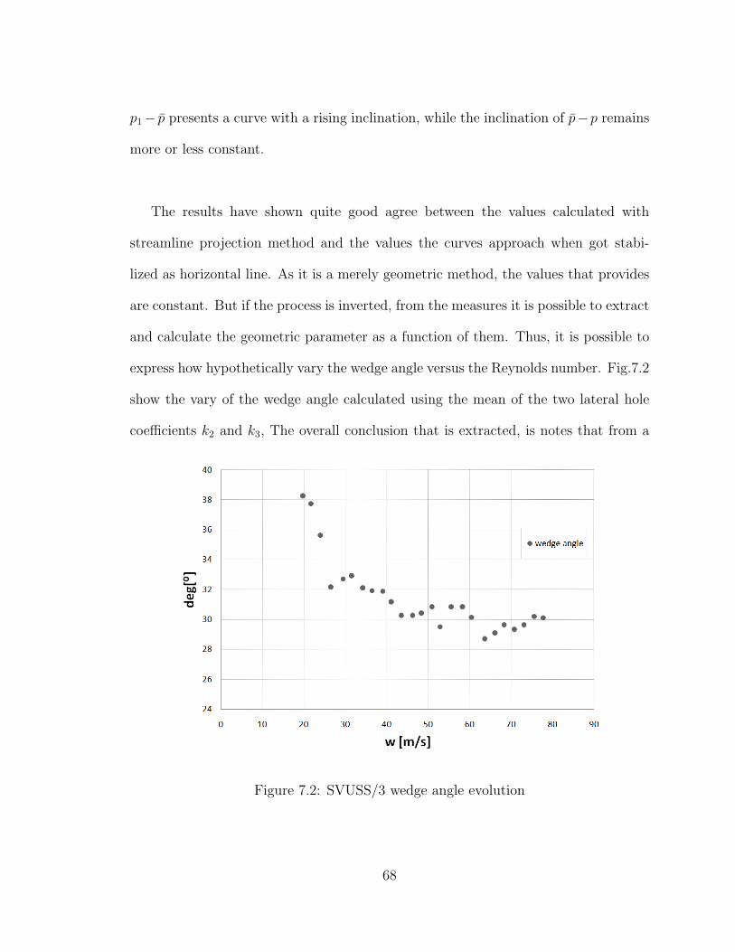
and calculate the geometric parameter as a function of them. Thus, it is possible to
express how hypothetically vary the wedge angle versus the Reynolds number. Fig.7.2
show the vary of the wedge angle calculated using the mean of the two lateral hole
coefficients k2 and k3, The overall conclusion that is extracted, is notes that from a
Figure 7.2: SVUSS/3 wedge angle evolution
68
certain speed, the wedge angle draws to its real value of δ = 30◦, and like the majority
of coefficients shows a negative trend. The explanation of this phenomena is because
at low Reynolds number a separation of the flow from the probe body is produced
on the surface of the two side holes, which create an alteration of the pressure sensed
by the outer holes. This phenomena was documented by Dominy and Hodson [1] as
a factor that has a significant influence on the calibration.
The dynamic pressure coefficient kd, which we suppose that it could display signs
that permit us to confirm the suspicious that hysteresis can appear during the ex-
periment, has not shown the expected results. The high degree of scatter makes that
although there is some transition zones represented like a slight deviation of the values
respect the natural trend, it is not evidence enough to affirm with certainty that it
would be hysteresis. Due to the dispersion at these zones looks like a cloud of points.
And there is no difference between those that were obtained increasing respect those
that were obtained decreasing the Reynolds number.
It is possible that was committed the original sin, to wait a concrete results before
carrying out the experiment. What has created some disappointment at not being
matched with the award expected. In view of the results obtained, has happened the
worst thing that could imagine, we cannot say with complete certainty nor deny that
the hysteresis is a factor to be taken into account in the calibration of the probes
used in this study. At the same time that it is not understood the big difference of
the results respect the calibration data provided by the manufacturer of SVUSS/3.
69
I propose therefore a modification in the method of calculating kd. Looking at
the equation that defines it Eq.(7.1). It depends of the coefficients k1 and k2. My
proposal is that instead of using only the coefficient k2, it would be more advisable
to use the average of both side coefficients k2 and k3. Because as it can be checked
at the previous chapter, even though the values of k2 and k3 should be equals due to
the symmetry of the probe, they are significantly. And the degree of scatter is also
different. Thus the formula must be the following,
kd =pt − pp1 − p
=1
k1 − k(7.1)
The aim of reduce the scatter and to have the absolute certainty that the mea-
surements are going correctly, the experiment was reproduced two times. And for one
probe even three times. Some modifications into the software of data acquisition were
introduced, decreasing the sampling frequency in order to obtain measures during a
longer time period. Thus is not necessary to take so many measures for each point,
so with 30 single measures is enough.
As is it said previously, the motor-fan velocity was set manually in increments of
50rpm in a range from 400 up to 1600rpm. But in order to test the software changes,
the experiment was repeated but this time setting the fan velocity in steps of 100rpm.
Under these new conditions the experimental data obtained were very clear, with a
low level of scatter.
Although is hard to imagine, with the yield results of the experiment, seems evident
that the human action of set the velocity of the fan has a substantial influence in
the scatter of the measures. There are no reasonable explanation of why there are
such a big difference between to set the velocity in steps of 50rpm instead of 100rpm.
70
Some hypothesis are possible, maybe it is be due to inertial factors of the motor that
actuate on the fan, or a supposed instability of the electronic system of DC that
regulate the velocity of the motor, or a error induced by human action while set the
velocity. At the last hypothesis, the effort of try to set the needle between two lines
of the indicator may cause an alternative movement of acceleration and deceleration
until find the concrete point. These facts make necessary a revision to try to improve
the method and the experimental procedure of data acquisition. At following lines
are explained some proposals of easy application which can provide important advan-
tages:
Instead of to work only with the mean of the measures for each point, save all the data
of the 30 measures done at each point. With them is possible to prepare a descriptive
statistic treatment of the data to obtain, furthermore of the mean, very important
parameters as standard deviation, maximum and minimum value measured. That
would permit to plot them over Reynolds number and analyze their variations.
The most important parameter of all of them and which provide more information
is the standard deviation. A high standard deviation indicates that the points are
far of the mean, and a low deviation indicates that the points are close to the mean.
Hence, it gives a degree of the stability of the flow field at the same time permit
identify transition zones from laminar (low deviations) to turbulent regimes (high
deviations). Also can be useful as an element to try to prove the hysteresis observed
in this work. Thus, a low standard deviation at this zone would mean that the degree
of scatter is low, thus the differences among increase and the progressive decrease of
the velocity are due to hysteresis.
71

Bibliography
[1] Dominy, R.G. and Hodson, H.P. An Investigation of Factors Influencing
the Calibration of Five-Hole Probes for Three-Dimensional Flow Measurements.
ASME Journal of Turbomachinery, Vol.115:513–519, 1993.
[2] Lee, S.W and Jun, B.J. Effects of Reynolds Number on the Non-Nulling
Calibration of a Cone-Type Five-Hole Probe. Proceedings of 2003 ASME TURBO
EXPO: Power for Land, Sea, Air, June 2003, Atlanta, USA.
[3] Lerena, D. and Willinger, R. Experimental Calibration of Three-Hole Pres-
sure Probes with Different Head Geometries.
[4] Mittal,S. and Saxena,P. Prediction of Hysteresis Associated with the Static
Stall of an Airfoil. AIAA Journal, Vol.35:933–935, 2000.
[5] Reneau,L.R., Johnston,J.P. and Kline,S.J. Performance and Design of
Straight, Two-Dimensional Diffusers. Journal of Basic Engineering, Transac-
tions of the ASME:141–150, March 1967.
[6] Schewe, G. Reynolds-number effects in flow around more-or-less bluff bodies.
Journal of Wind Engineering and Industrial Aerodynamics, Vol.89:1267–1289,
2001.
72
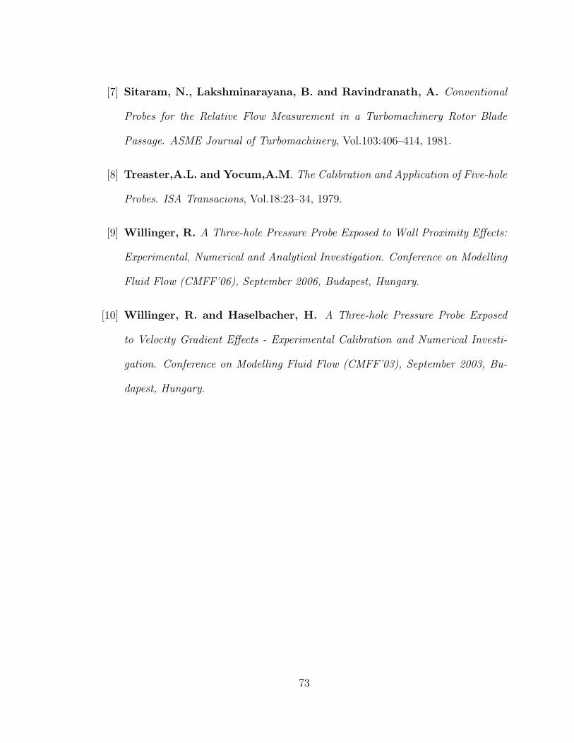
[7] Sitaram, N., Lakshminarayana, B. and Ravindranath, A. Conventional
Probes for the Relative Flow Measurement in a Turbomachinery Rotor Blade
Passage. ASME Journal of Turbomachinery, Vol.103:406–414, 1981.
[8] Treaster,A.L. and Yocum,A.M. The Calibration and Application of Five-hole
Probes. ISA Transacions, Vol.18:23–34, 1979.
[9] Willinger, R. A Three-hole Pressure Probe Exposed to Wall Proximity Effects:
Experimental, Numerical and Analytical Investigation. Conference on Modelling
Fluid Flow (CMFF’06), September 2006, Budapest, Hungary.
[10] Willinger, R. and Haselbacher, H. A Three-hole Pressure Probe Exposed
to Velocity Gradient Effects - Experimental Calibration and Numerical Investi-
gation. Conference on Modelling Fluid Flow (CMFF’03), September 2003, Bu-
dapest, Hungary.
73