difference map and its electronic circuit realization

Nonlinear Dyn (2013) 74:819–830DOI 10.1007/s11071-013-1007-4

O R I G I NA L PA P E R

Difference map and its electronic circuit realization

M. García-Martínez · I. Campos-Cantón ·E. Campos-Cantón · S. Celikovský

Received: 24 January 2013 / Accepted: 10 July 2013 / Published online: 3 August 2013© Springer Science+Business Media Dordrecht 2013

Abstract In this paper we study the dynamical behav-ior of the one-dimensional discrete-time system, theso-called iterated map. Namely, a bimodal quadraticmap is introduced which is obtained as an amplifica-tion of the difference between well-known logistic andtent maps. Thus, it is denoted as the so-called differ-ence map. The difference map exhibits a variety of be-haviors according to the selection of the bifurcationparameter. The corresponding bifurcations are studiedby numerical simulations and experimentally. The sta-

M. García-Martínez (B) · E. Campos-CantónDivision de Matemáticas Aplicadas, Instituto Potosino deInvestigación Científica y Tecnológica, Camino a la PresaSan José 2055, 78216 México, Méxicoe-mail: [email protected]

I. Campos-CantónFacultad de Ciencias, Universidad Autónoma de San LuisPotosí, Zona universitaria, Avenida Salvador Nava S/N,78290 México, Méxicoe-mail: [email protected]

E. Campos-CantónDepartamento de Físico Matemáticas, UniversidadAutónoma de San Luis Potosí, Zona universitaria, AvenidaNiño Artillero S/N, 78290 México, Méxicoe-mail: [email protected]

S. CelikovskýDepartment of Control Theory, Institute of InformationTheory and Automation, Academy of Sciences of theCzech Republic, Pod vodárenskou veží 4, 18208 Prague,Czech Republice-mail: [email protected]

bility of the difference map is studied by means ofLyapunov exponent and is proved to be chaotic ac-cording to Devaney’s definition of chaos. Later on, adesign of the electronic implementation of the differ-ence map is presented. The difference map electroniccircuit is built using operational amplifiers, resistorsand an analog multiplier. It turns out that this elec-tronic circuit presents fixed points, periodicity, chaosand intermittency that match with high accuracy to thecorresponding values predicted theoretically.

Keywords Chaotic behavior · Lyapunov exponent ·Bifurcation parameter · Bifurcation diagram ·Stability analysis

1 Introduction

Iterated maps are simple looking discrete-time dynam-ical systems which can exhibit transitions from orderto chaos. Famous and broadly studied examples of uni-modal maps are the tent map and the logistic map, be-ing the subject of constant investigation in many ar-eas such as communication systems [1], generation ofpseudo-random sequences [2–4], neural networks [5],switching systems [6] and cryptography [7–11] andpart of the interest for these systems is linked to thefact that they provide an easy and academic way to un-derstand how complex and chaotic behavior can arisefrom simple dynamical models. Even more remark-able is the fact that studies of low-dimensional maps

mailto:[email protected]




820 M. García-Martínez et al.

have proven to be profitable in understanding the basicmechanisms responsible for the appearance of chaosin a large class of dynamical systems.

Furthermore complex behavior may be provided bythe so-called bimodal, or even k-modal maps, [12].This paper introduces yet another bimodal map, basedon the difference between logistic and tent maps mul-tiplied by a new bifurcation parameter. This new sys-tem is therefore called the difference one and is care-fully analyzed theoretically, numerically and experi-mentally through electronic circuit.

One of the most useful and widely accepted defi-nition of chaos is the given by Devaney [13], whichwe will call Devaney-chaos. Roughly speaking, threeconditions are required, (1) the sensitive dependenceupon the initial condition, (2) the topological transitiv-ity, and (3) the dense distribution of the periodic orbits.The third condition is often omitted for being too strin-gent [14]. Fortunately, there are other ways to char-acterize the dynamic behavior, like the result of Li–Yorke [15] which can be used to prove the existenceof chaos in a map, the authors state that if there ex-ists a point of period three then there exist points withother periods and the system is chaotic. On the otherhand we have the Lyapunov exponents [16–18]. Withthe aid of their diagnostic, one can measure the av-erage exponential rates of divergence or convergenceof nearby orbits in the phase space. In general, singsof the Lyapunov exponents give a qualitative idea ofthe variety of dynamics that may exhibit, ranging fromfixed points via limit cycles and tori to more com-plex chaotic attractors. Also, bifurcation diagrams areexcellent tools to study dynamical behavior and un-derstand mechanisms such as the so-called a cascadeof period-doubling bifurcations, encountered qualita-tively in many physical systems of interest or math-ematical models that have been electronically imple-mented [19, 20].

Electronic implementation of chaotic systems havebeen applied to several engineering developments, fur-thermore they have been of great help to validatecertain theories concerning chaos. Since its incep-tion three decades ago, there are different implemen-tations of Chua’s circuit [21–23]. Historically seen,Chua’s circuit was the first successful physical imple-mentation of a system designed to exhibit chaos [24].This circuit is the first system rigorously proved tobe chaotic [25]. Chua’s circuit is a continuous-timedynamical system where chaos can be observed ex-

perimentally. The original Chua’s system has a dou-ble scroll but the diode has been modified in orderto generate chaotic multi-scroll [26]. The behavior ofthe difference map is simpler than Chua’s circuit tocomprehend and it has been proved chaotic. The be-havior of Chua’s oscillator is due to the fact that itcontains five different parameters, whereas for dif-ference map is only one. There have been reportedseveral electronic implementations of continuous-timedynamical systems, such systems are based on third-order differential equations see [27–31], but few inthe area of discrete-time dynamical systems. Further-more, discrete-time dynamical systems present advan-tage and be useful in applications like encryption sys-tems, radar systems, secure communication systems,among others.

Some discrete dynamical systems have been imple-mented by using digital integrated circuits, for exam-ple in [32] presents a digital implementation of the tentmap. The problem that arises using digital implemen-tation is that the system only takes a finite number ofstates. Electronic circuits have been designed, imple-mented and tested to accurately realize the logistic dif-ference equation [19] or the tent-map difference equa-tion [20] by using analog devices in order to have aninfinite number of values that can be visited.

In this paper, we enlarge the set of maps known tobe chaotic by presenting a chaotic map based on thedifference between the logistic map and the tent map.The difference map, more precisely, enables us to con-struct a bimodal map which is chaotic in the sense thatit has positive Lyapunov exponent. We also present anelectronic implementation of the difference map basedon analog devices, which at the same time is a goodengineering model of the corresponding mathematicalsystem. Through the variation of only one control pa-rameter, one can examine the bifurcation diagram ofthe realized system and we have been able to repro-duce the theoretical diagram with high accuracy.

The possible application of this circuit implemen-tation would be independent analog chaos generatorusable for encryption purposes, e.g. as independentdevice to cipher. In recent years, a growing numberof cryptosystems based on continuous systems utilizethe idea of synchronization of chaos. However, recentstudies show that the performance of continuous sys-tems is very poor and insecure. The insecurity resultsmainly from the insensitivity of synchronization tosystems parameters [33–36] i.e., the synchronization

Difference map and its electronic circuit realization 821

of a pair of chaotic systems is possible even if theyhave mismatch parameters.

This paper is organized as follows. In the next sec-tion we recall some basic definitions; while Sect. 3 in-troduces the difference map, including its theoreticaland numerical study and presents its properties. Sec-tion 4 contains a description of an electronic circuitimplementation of the difference map and the experi-mental bifurcation diagram which matches the theoret-ically predicted results. Some conclusions and outlookare given in the final section.

2 Basic definitions

This paper aims to contribute in the area of the one-dimensional discrete-time systems, namely to the sys-tems of the form

xk+1 = f (xk), k = 0,1,2, . . . ,N.

Here xk ∈ � and x0 is the initial condition, such dy-namical system is usually called a map, as it is fullydetermined by its right hand side. To ensure bounded-ness of trajectories, the study is usually restricted tomaps that are mapping some closed interval into it-self and without any loss of generality one may con-sider the closed interval [0,1] only. The simplest mapsare the so-called unimodal maps, while their general-ization, the so-called k-modal maps may present evenmore rich dynamical behaviors, [12].

To be more specific, denote I := [0,1] and recallthat the critical point c of the continuous piecewisesmooth map f (x) : I �→ I is c ∈ I where f is differ-entiable and f ′(c) = 0.

Remark 1 The critical point c occurs for f ′(c) = 0or f ′(c) does not exist. But continuous smooth mapsalways present f ′(c) = 0.

First, let us repeat the definition of the k-modalmap, introduced in [12].

Definition 1 The map f : I �→ I is called the k-modal one, if it is continuous on I and it has k criticalpoints denoted by c0, c1 , . . . , ck−1 in I . Moreover,there exist intervals Ii , i = 0, . . . , k − 1,

⋃ki=1 Ii−1 =

I , such that ∀i = 0, . . . , k − 1 it holds ci ∈ Ii andf (ci) > f (x,β), ∀x ∈ Ii and x �= ci , where β is a pa-rameter. The case k = 1 will be further simply referred

as to the so-called unimodal map, while the case k = 2as the bimodal one.

Remark 2 The above definition does not constrain afunction to have only k critical points. However weonly considered those that are local maxima on asubinterval.

Definition 2 The logistic map is defined as

fL(x,α) = αx(1 − x), (1)

where parameter α ∈ [0,4] ⊂ �.

The logistic map was first presented by Verhulst[37] as a model for the growth of species and it is oneof the classical dynamical systems. The logistic maphas been extensively studied and other properties canbe found in [38] while some basic properties can befound in [39, 40].

Definition 3 The tent map is defined as

fT,(x,μ) ={

μx, for x < 1/2,

μ(1 − x), for x ≥ 1/2,(2)

where parameter μ ∈ [0,2] ⊂ �.

The logistic and tent maps are obviously unimodalones, as they are continuous on I with a single crit-ical point c0 = 0.5 and they increase for x ∈ [0,0.5)

and they decrease for x ∈ [0.5,1]. Their bifurcationdiagrams using α and μ as control parameters demon-strate a very rich dynamics [41, 42].

Example 1 The following quadratic map:

fQ(x, γ ) = γ (1 − 2x)

{x, if x < 0.5,

(x − 1), other case,(3)

is the bimodal map in the sense of the Definition 1.As a matter of fact, the map given by Eq. (3) hasthree critical points and two of them are c0 = 0.25 andc1 = 0.75 located at intervals I0 = [0,0.5) and I1 =[0.5,1], respectively. The other critical point c = 0.5due to f ′

Q(0.5) does not exist. Notice that this criticalpoint does not satisfied the Definition 1. Thus the mapgiven by Eq. (3) is a bimodal map.


Fig. 1 Difference map for different valued of β: 1.333 (lineformed by circles), 2.666 (dotted line) and 4 (line formed bytriangles)

Definition 4 (Devaney’s Definition of Chaos) [14] Let(X;d) be a metric space. Then, a map f : X → X issaid to be Devaney-chaotic on X if it satisfies the fol-lowing conditions.

1. f has sensitive dependence on initial conditions.That is, there exists a certain ε > 0 such that,for any x ∈ X and δ > 0, there exists some y ∈X where the distance d(x;y) < δ and m ∈ ℵ ={1,2,3, . . .} so that the distance d(f m(x);f m(y)) > ε.

2. f is topologically transitive. That is, for any pairof open sets U,V ⊂ X, there exists a certain m ∈ ℵsuch that f m(U)

⋂V �= ∅.

3. f has dense distribution of the periodic orbits. Thatis, suppose Y is the set that contains all periodicorbits of f , then for any point x ∈ X, there is apoint y in the subset Y arbitrarily close to x.

The concept of neighborhood of a point x ∈ X isimportant for demonstrating the second condition ofDevaney’s definition of chaos and is given as follows.

Definition 5 A neighborhood of a point x ∈ X is aset Nδ(x) consisting of all points y ∈ X such that thedistance d(x, y) < δ. The number δ is called the radiusof Nδ(x).

3 Difference map

The main contribution of this paper is to present theso-called difference map and to provide its implemen-tation as an electronic circuit. The difference map, de-noted as fD(x,β), will be a particular case of the

Fig. 2 Stability of the fixed points. The asterisks and circlesdenote stable and unstable fixed points, respectively

above described bimodal quadratic map equation (3)denoted fQ(x, γ ) : [0,1] → [0,1] with γ = 2β , whereparameter β ∈ [0,4] ⊂ �. This difference map is con-structed based on the difference between logistic mapand tent map, which explains such a terminology.More precisely, consider the following.

Definition 6 Consider the logistic and tent maps withmaximum bifurcation parameters α = 4, μ = 2, re-spectively. Defined fD(x,β) as the difference betweenthese two maps multiplied by the parameter β ∈ [0,4],namely, fD(x,β) = β(fL(x,4) − fT (x,2)), i.e.:

fD(x,β) ={

2βx(1 − 2x), for x < 12 ;

2β(x − 1)(1 − 2x), for x ≥ 12 .

(4)

Indeed, the difference map defined in the Defini-tion 6 is exactly the bimodal map equation (3) withγ = 2β . Now, β is a new bifurcation parameter whichamplifies the difference between the logistic map andthe tent map. This new parameter belongs to the in-terval [0,4], notice that for β = 4 the difference mapfD(x,β) : [0,1] → [0,1]. Figure 1 shows the differ-ence map given by Eq. (4) for different values of β:1.333 (line formed by circles), 2.666 (dotted line) and4 (line formed by triangles). Notice that the differ-ence map always has a fixed point at 0 and it canhave others depending on the value of β at 2β−1

4β,

6β−1−√

4β2−12β+18β

and 6β−1+√

4β2−12β+18β

.To analyze the behavior of the discrete-time dy-

namical system we put the map as its right hand side,


Fig. 3 Bifurcation diagram for the difference map givenby Eq. (4)

i.e. the system

xk+1 =fD(xk,β), for x0 given and k = 0,1,2,3, . . .

The difference map can behave as a bimodal orunimodal map according to the β bifurcation param-eter value. For example, if β = 2, then for any initialcondition x0 ∈ [0,1], fD(x,β) behaves after the firstiteration as an unimodal map fD(x,β) : [0,0.5] →[0,0.5]. The stability of fixed points of the differencemap can be attractive or repulsive as is shown in Fig. 2.An asterisk denotes an attractive fixed point and a cir-cle denotes a repulsive fixed point. The fixed point lo-cated at zero is attractive for β ∈ [0,0.5) and repul-sive for β ∈ [0.5,4]. The second fixed point is givenby 2β−1

4βwhich is attractive for β ∈ [0.5,1.495) and

repulsive for β ∈ [1.495,4]. The third fixed point lo-

cated at 6β−1−√

4β2−12β+18β

is always repulsive for β ∈[2.915,4] and last one given by 6β−1+

√4β2−12β+18β

is attractive for β ∈ [2.915,3.235) and repulsive forβ ∈ [3.235,4].

It is well known that an attractive fixed point doesnot let oscillations meanwhile a repulsive fixed pointcan yield periodic orbits and even chaotic orbits. Fig-ure 3 shows a bifurcation diagram of the orbit of thedifference map fD(x0, β), which is on [0,1] × [0,4].Two sequences of the period-doubling bifurcations ap-pear approximately at β = 1.5 and β = 3.2312. Forβ ∈ [0,2] the difference map resembles to the logis-tic map but it oscillates in the interval [0,0.5], and for

Fig. 4 Lyapunov exponent of the difference map

β ∈ [2,4] it behaves as a bimodal map and it can os-cillate in the interval [0,1].

The Lyapunov exponent, which is denoted by λ,gives the global stability of the system equation (3)and it is shown in Fig. 4. For β ∈ [0,0.5] the systemonly has a fixed point which is attractive and λ < 0, theorbit converges to the fixed point. For β ∈ [0.5,1.5)

the system has two fixed points: one attractive andthe other repulsive and λ < 0 due to the orbit con-verges to the attractive fixed point but when β = 1.5the system has a bifurcation and the value of λ = 0.For β ∈ (1.5,2.915) the system has two fixed pointsand both are repulsive and λ < 0 when the orbit pe-riodically oscillates or λ > 0 when the orbit oscillateschaotically. For β ∈ (2.915,3.235) the system has fourfixed points and three of them are repulsive and theother fixed point is attractive, λ < 0, thus the orbitconverges to the attractive fixed point again and alsowhen β = 3.235 another bifurcation occurs and there-fore λ = 0. For β ∈ (3.235,4] the system maintainsits four fixed points but now all of them are repulsive.The orbit oscillates periodically or chaotically whenλ < 0 and λ > 0, respectively. It is worth mentioningthat the Lyapunov exponent was defined for unimodalsystems; however, it measures the average exponentialrates of divergence or convergence of orbits no mat-ter if the system is k-modal because the system is onedimensional.

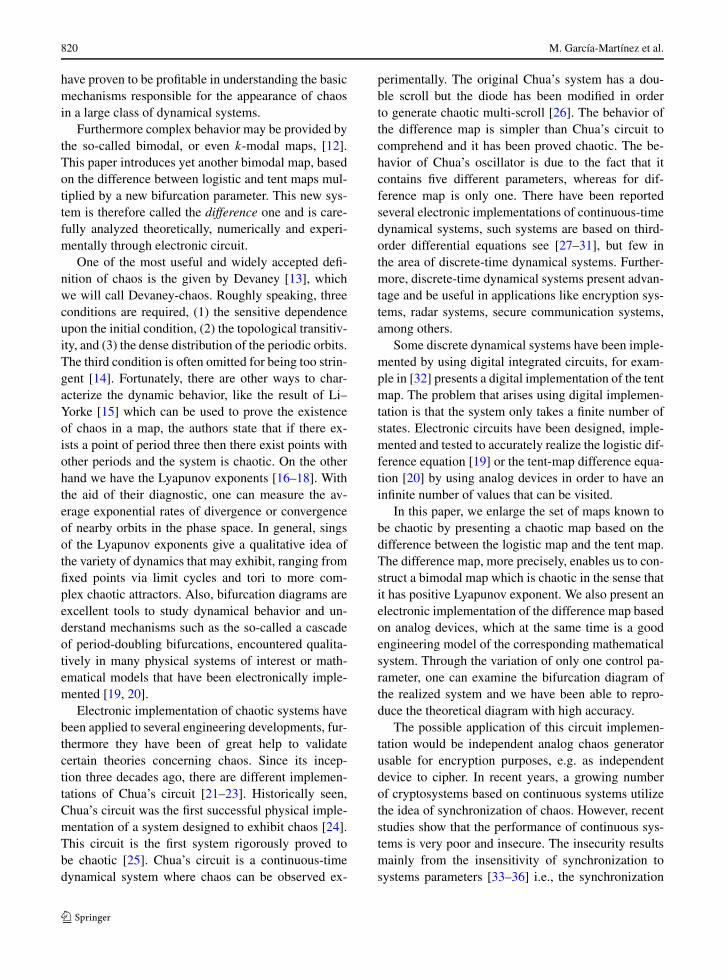
Theorem 1 The difference map fD(x,β) is Devaney-chaotic on [0,1] for β = 4.


Fig. 5 The difference map and the subintervals J 1i , i = 0,

1,2,3. Circles denote critical points, squares denote fixed pointsand triangles denote η

Proof From Definition 4, we need to prove three con-ditions: (1) the sensitive dependence upon the initialcondition, (2) the topological transitivity and (3) thedense distribution of the periodic orbits.

We start by demonstrating the last property. Weneed to prove that there exists a Y subset of the inter-val I = [0,1] constitutes for periodic orbits, and thatY is dense in I . The I interval can be divided by J 1

0 =[0, c1

0], J 11 = [c1

0, η00 = 0.5], J 1

2 = [η00 = 0.5, c1

1] andJ 1

3 = [c11,1] (see Fig. 5), and each intervals contains

one fixed point of the difference map fD , Δ1 = {p10 =

0,p11 = 0.4375,p1

2 = 0.5899,p13 = 0.8476}, respec-

tively. These fixed points in the closed interval I be-long to Y as periodic orbits of period one, wherec1

0 = 0.25 and c11 = 0.75 are the critical points. Notice

that fD : J 1i → [0,1], i = 0, . . . ,3, then each subinter-

val resembles the difference map for f 2D . Notice that

fD(0) = fD(0.5) = fD(1) = 0 and fD(c10 = 0.25) =

fD(c11 = 0.75) = 1. The foregoing observation let us

to infer that for all x ∈ I and if f kD(x) = 0.5 then

f k+1D (x) = 0.

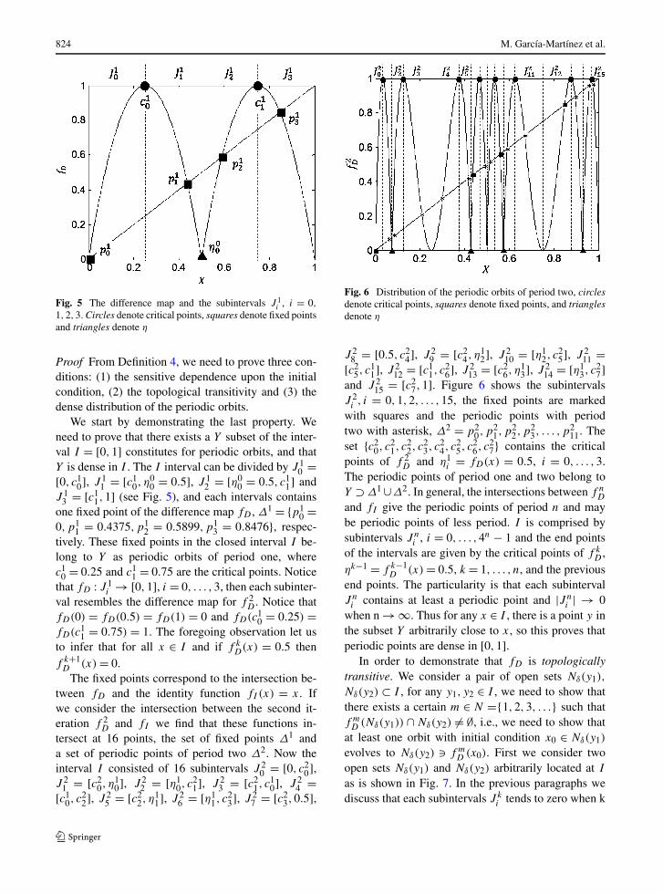
The fixed points correspond to the intersection be-tween fD and the identity function fI (x) = x. Ifwe consider the intersection between the second it-eration f 2

D and fI we find that these functions in-tersect at 16 points, the set of fixed points Δ1 anda set of periodic points of period two Δ2. Now theinterval I consisted of 16 subintervals J 2

0 = [0, c20],

J 21 = [c2

0, η10], J 2

2 = [η10, c

21], J 2

3 = [c21, c

10], J 2

4 =[c1

0, c22], J 2

5 = [c22, η

11], J 2

6 = [η11, c

23], J 2

7 = [c23,0.5],

Fig. 6 Distribution of the periodic orbits of period two, circlesdenote critical points, squares denote fixed points, and trianglesdenote η

J 28 = [0.5, c2

4], J 29 = [c2

4, η12], J 2

10 = [η12, c

25], J 2

11 =[c2

5, c11], J 2

12 = [c11, c

26], J 2

13 = [c26, η

13], J 2

14 = [η13, c

27]

and J 215 = [c2

7,1]. Figure 6 shows the subintervalsJ 2

i , i = 0,1,2, . . . ,15, the fixed points are markedwith squares and the periodic points with periodtwo with asterisk, Δ2 = p2

0,p21,p

22,p

23, . . . , p

211. The

set {c20, c

21, c

22, c

23, c

24, c

25, c

26, c

27} contains the critical

points of f 2D and η1

i = fD(x) = 0.5, i = 0, . . . ,3.The periodic points of period one and two belong toY ⊃ Δ1 ∪Δ2. In general, the intersections between f n

D

and fI give the periodic points of period n and maybe periodic points of less period. I is comprised bysubintervals Jn

i , i = 0, . . . ,4n − 1 and the end pointsof the intervals are given by the critical points of f k

D ,ηk−1 = f k−1

D (x) = 0.5, k = 1, . . . , n, and the previousend points. The particularity is that each subintervalJn

i contains at least a periodic point and |Jni | → 0

when n → ∞. Thus for any x ∈ I , there is a point y inthe subset Y arbitrarily close to x, so this proves thatperiodic points are dense in [0,1].

In order to demonstrate that fD is topologicallytransitive. We consider a pair of open sets Nδ(y1),

Nδ(y2) ⊂ I , for any y1, y2 ∈ I , we need to show thatthere exists a certain m ∈ N ={1,2,3, . . .} such thatf m

D (Nδ(y1)) ∩ Nδ(y2) �= ∅, i.e., we need to show thatat least one orbit with initial condition x0 ∈ Nδ(y1)

evolves to Nδ(y2) � f mD (x0). First we consider two

open sets Nδ(y1) and Nδ(y2) arbitrarily located at I

as is shown in Fig. 7. In the previous paragraphs wediscuss that each subintervals J k

i tends to zero when k


Fig. 7 There exists an orbit such that two points with a neigh-borhood comes arbitrarily close

Fig. 8 Transitivity of an orbit of period n (f nD) of difference

map

tends to infinity, also we know that each subinterval J ki

is mapped onto the interval I , f kD : J k

i → I . Thus,consider a subinterval Jm

i ⊂ Nδ(y1). as is shown inFigs. 8 and 9. Accordingly f (Jm

i ) = I ⊃ Nδ(y2) thenf m

D (x0) ∈ Nδ(y2), for any x0 ∈ Nδ(y1), this proves thatfD is topologically transitive.

Finally, we need to demonstrate sensitive depen-dence on initial conditions of the difference map, sothat we start to define ε = |I |/2, where |I | = 1, suchthat for any x01 ∈ I and any δ > 0 there is a x02 ∈Nδ(x01) such that the distance between |f m

D (x01) −f m

D (x02)| ≥ ε.So if we consider the subinterval Jm−1

i such thatJm−1

i ⊂ Nδ(x01) then there is a x02 ∈ Jm−1i such that

Fig. 9 A zoom of Fig. 8 in order to appreciate the transitivityof an orbit of period n where f (Jm

i ) ⊇ I ⊃ Nδ(y1)

Fig. 10 Circuit diagram of an electronic map

|f mD (x01) − f m

D (x02)| ≥ 1/2. Thus we have sensitivedependence on initial conditions is important to notethat the definition of sensitivity does not require thatthe orbit of x02 remains far from x01 for all iterations.We only need one point on the orbit to be far from thecorresponding iterate of x01.

Now the proof is completed. �

Remark 3 The Li–Yorke theorem can be used todemonstrate chaos, but for the purposes of this paperTheorem 1 is sufficient.

4 Electronic implementation of the difference map

An electronic circuit of a discrete map is made upby the implementation of two parts: (1) the discretemap circuit, and (2) the iterative process circuit, see


Fig. 11 Block diagram ofthe difference map used toconstruct the electroniccircuit

Fig. 10. Some electronic implementations are basedon microprocessor or microcontrollers in one or bothof its parts; however this leads to a discrete space.From Definition 4, one can immediately see that nomap is Devaney-chaotic if X is a discrete space. Thus,a chaotic system needs to be implemented electron-ically by analog devices. First we will focus on ex-plaining the circuit of the difference map.

The experimental development of this map isachieved by means of electronic devices as multipli-ers, operational amplifiers, diodes, and resistors. Inthe same spirit that other implementations of this kindof circuits [19, 43] analog multipliers have been em-ployed with a normalization of the signal by a factorof about 10. This normalization is necessary becauseof the physical restrictions in the analog multiplier.The starting point is a block diagram of the differ-ence map that is shown in Fig. 11. The output of theelectronic circuit has three branches: The first gener-ates the logistic map (node A) and the last two corre-spond to the tent map (node B and C). Typically, thesecircuits contain several operational amplifiers, which

perform linear operations (e.g., integration and sum-mation), as well as a couple of integrated circuits thatperform the nonlinear operations (i.e., multiplication).Here, we describe a new circuit contains active com-ponents, speeds of radio frequencies, and is capable ofreproducing the transition from steady state to chaosas observed in the difference map equation when thebifurcation parameter is varied.

Figure 12 shows a schematic diagram of the elec-tronic circuit realization of the difference map. Theoutput of the circuit is analyzed using the voltages atthe nodes: A, B, C, D.

The A node voltage is given by the M1 multiplierwhich has four input terminals (x1, x2, y1, y2) and anoutput terminal given by W = (x1−x2)(y1−y2)

10 . Inputsx1 = Vin(R2R4)/(R1R3) and y2 = Vin(R2R6)/(R1R5)

are given by operational amplifiers U2 and U3, respec-tively. Inputs x2 and y1 are 0 V and 5 V, respectively.Hence, the output at A node is given by

VA =(

VinR2R4

R1R3

)(

5 − VinR2R6

R1R5

)

/10, (5)


Fig. 12 Schematic diagramof the difference mapelectronic circuit

the A node voltage is Vin(1 − Vin) after evaluatingcomponents values of the Table 1, this signal corre-sponds to the logistic map fL without considering theα bifurcation parameter.

The B node voltage is given by the U4 amplifieroutput which is fed back to the inverting input, the out-put voltage is

VB = −VinR13/R12. (6)

The C node voltage is given by the U5 amplifieroutput which is a piecewise linear signal, then

VC ={

0, for Vin < R72R8

;R11R10

(R9VinR7

− R92R8

), for Vin ≥ R72R8

.(7)

Equations (6) and (7) correspond to the tent map,remember that fT (x,μ) is defined by two parts, to en-sure that the map is symmetric the bifurcation param-eter μ must be the same on both sides. We can see thatμ is given by R13/R12 and R11/(2R10). This yieldsthe following restrictions: R11 = 2R13 and R10 = R12.

The U7 amplifier output is the adding of A, B andC node voltages which correspond to D node voltage,giving

VD = −R17

(VA

R16+ VB

R15+ VC

R14

)

, (8)

it is worth mentioning that the ratio R17/R16 isthe parameter α = 4. Thus, the D node voltage is(−fL + fT ) that is indeed the difference map invested


Table 1 The values of the electronic components employed inthe construction of the difference map electronic circuit

Device Value

R1,R3,R5,R6,R7,R8,R9,

R10,R12,R16,R18 10 k Resistor

R4 4 k Resistor

R11,R14,R15,R17 40 k Resistor

R13 20 k Resistor

R19 40 k Potentiometer

D1, D2 1N4148 Diode

U1, U2, U3, U4, U5, U6, U7, U8 TL084 Op. Amp.

M1 AD633 Multiplier

without taking into account the bifurcation parame-ter β .

Finally, the Vout voltage is given by the U8 invertingamplifier, the output is (R19/R18)VD . Assuming idealperformance from all components, the circuit outputin Fig. 12 is modeled by the following equation:

Vout = R19

R18

⎧⎪⎨

⎪⎩

4Vin(1− Vin) − 2Vin, forVin < 12 V;

4Vin(1− Vin) + 2Vin − 2,

forVin ≥ 12 V.

(9)

Then, Eq. (4) can be derived from Eq. (9) by thechange of variables Vin = xn, Vout = xn+1 and β =R19/R18.

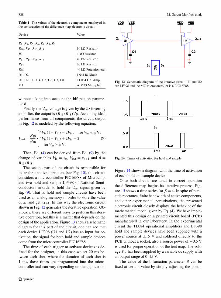
The second part of the circuit is responsible formake the iterative operation, (see Fig. 10), this circuitconsiders a microcontroller PIC16F88 of Microchip,and two hold and sample LF398 of National Semi-conductors in order to hold the Vout signal given byEq. (9). That is, hold and sample circuits have beenused as an analog memory in order to store the valueof xk and get xk+1. In this way the electronic circuitshown in Fig. 12 generates the iterative operation. Ob-viously, there are different ways to perform this itera-tive operation, but this is a matter that depends on thedesign of the application. Figure 13 shows a schematicdiagram for this part of the circuit, one can see thateach device LF398 (U1 and U2) has an input for ac-tivation, the signal for both hold and sample devicescome from the microcontroller PIC16F88.

The time of each trigger to activate devices is de-fined for the designer, in this case we set 20 ms be-tween each shot, where the duration of each shot is1 ms, these times are programmed into the micro-controller and can vary depending on the application.

Fig. 13 Schematic diagram of the iterative circuit, U1 and U2are LF398 and the MC microcontroller is a PIC16F88

Fig. 14 Times of activation for hold and sample

Figure 14 shows a diagram with the time of activationof each hold and sample device.

Once both circuits are tuned in correct operationthe difference map begins its iterative process. Fig-ure 15 shows a time series for β = 4. In spite of para-sitic reactance, finite bandwidth of active components,and other experimental perturbations, the presentedelectronic circuit closely displays the behavior of themathematical model given by Eq. (4). We have imple-mented this design on a printed circuit board (PCB)manufactured in our laboratory. In the experimentalcircuit the TL084 operational amplifiers and LF398hold and sample devices have been supplied with apower source at ±15 V and soldered directly to thePCB without a socket, also a source power of −0.5 Vis used for proper operation of the tent map. The volt-age Vdc has been supplied by a variable dc supply withan output range of 0–15 V.

The value of the bifurcation parameter β can befixed at certain value by simply adjusting the poten-


Fig. 15 The time series with chaotic dynamics generated by thetent map for β = 4

Fig. 16 Experimental bifurcation diagram for the differencemap

tiometer R19 located in the operational amplifiers U8.In order to explore the full range of the dynamics ac-cessible to this circuit, we have experimented with dif-ferent values for R19. The value of this potentiometerhas been adjusted in the closed interval [0 ,40 k].Then the value of β has been varied to obtain the bifur-cation diagram shown in Fig. 16, where fixed points,periodic oscillations, cascade of period-doubling bi-furcations and chaos can be clearly seen. It is possi-ble to see that the circuit exhibits the entire range ofbehaviors of the difference map. In fact, our experi-mental results of the dynamics of this circuit are foundto be in good agreement with numerical simulations.

Note that this circuit only produce a bimodal mapin order to construct a circuit with k modal we need touse another technique as comparator circuits in orderto define the partition of the space and after this con-struct a logistic map on each partition using multipliersdevices.

5 Conclusion

In this paper we introduced a new discrete-time dy-namical system of one dimension based on the differ-ence of the logistic and tent map. This map is a bi-modal map that presents chaotic behavior according

to its Lyapunov exponent. One of the main proper-ties of this map is that it can show the behavior of aunimodal map or a bimodal map by setting the β pa-rameter. A difference map electronic circuit has beenpresented here and its implementation using only ana-log components as operational amplifiers, multipliers,diodes, and resistors was also provided. Thus, this de-sign can be manufactured in just one chip becausethe final electronic circuit contains only semiconduc-tors and passive components. Its experimental behav-ior was tested and compared with the numerical be-havior given by the difference map equation 4. Thecircuit replicates the whole known range of behaviorsof the difference map and it has many potential appli-cations, for example: random number generation, fre-quency hopping, ranging, and spread-spectrum com-munications. As the outlook for further research, thepossibility of encryption using stream ciphers basedon the analog circuit is considered. This is the objectof currently ongoing research.

Acknowledgements M. García-Martínez is a doctoral fel-lows of CONACYT (Mexico) in the Graduate Program on Con-trol and Dynamical Systems at DMAp-IPICYT.

E. Campos-Cantón acknowledges CONACYT for the finan-cial support through project No. 181002.

S. Celikovský has been supported by the Czech ScienceFoundation through the research grant no. 13-20433S.

References

1. Mengue, A.D., Essimbi, B.Z.C.: Secure communication us-ing chaotic synchronization in mutually coupled semicon-ductor lasers. Nonlinear Dyn. 70(2), 1241–1253 (2012)

2. Wang, X.-y., Qin, X., Jessa, M.: A new pseudo-randomnumber generator based on CML and chaotic iteration.Nonlinear Dyn. 70, 1589–1592 (2012)

3. Patidar, V., Sud, K.K., Pareel, N.K.: A pseudo random bitgenerator based on chaotic logistic map and its statisticaltesting. Informatica 33, 441–452 (2009)

4. Yuan, X., Xie, Y.-X.: A design of pseudo-random bit gen-erator based on single chaotic system. Int. J. Mod. Phys. C23(3), 1250024 (2012)

5. Zou, A.-M., Kumar, K.D., Pashaie, R., Farhat, N.H.: Neuralnetwork-based adaptive output feedback formation controlfor multi-agent systems. Nonlinear Dyn. 70, 1283–1296(2012)

6. Chen, Y., Fei, S., Zhang, K.: Stabilization of impulsiveswitched linear systems with saturated control input. Non-linear Dyn. 69, 793–804 (2012)

7. Mazloom, S., Eftekhari-Moghadam, A.M.: Color image en-cryption based on coupled nonlinear chaotic map. ChaosSolitons Fractals 42, 1745–1754 (2009)


8. Shatheesh Sam, I., Devaraj, P., Bhuvaneswaran, R.S.: Anintertwining chaotic maps based image encryption scheme.Nonlinear Dyn. 69, 1995–2007 (2012)

9. Farschi, S.M.R., Farschi, H.: A novel chaotic approach forinformation hiding in image. Nonlinear Dyn. 69, 1525–1539 (2012)

10. Hussain, I., Shah, T., Gondal, M.A.: Image encryption al-gorithm based on PGL(2,GF(28)) S-boxes and TD-ERCSchaotic sequence. Nonlinear Dyn. 70, 181–187 (2012)

11. Kwok, H.S., Tang, W.K.S.: A fast image encryption systembased on chaotic maps with finite precision representation.Chaos Solitons Fractals 32, 1518–1529 (2007)

12. Campos-Cantón, E., Femat, R., Pisarchik, A.N.: A fam-ily of multimodal dynamic maps. Commun. Nonlinear Sci.Numer. Simul. 9, 3457–3462 (2011)

13. Devaney, R.: An Introduction to Chaotic Dynamical Sys-tems, 2nd edn. Westview Press, Boulder (2003)

14. Kahng, B.: Redefining chaos: Devaney-chaos for piecewisecontinuous dynamical systems. Int. J. Math. Models Meth-ods Appl. Sci. 3(4), 317–326 (2009)

15. Li, T.-Y., Yorke, J.A.: Period three implies chaos. Am.Math. Mon. 82(10), 985–992 (1975)

16. Li, C., Chen, G.: Estimating the Lyapunov exponents of dis-crete systems. Chaos 14, 343–346 (2004)

17. Sano, M., Sawada, Y.: Measurement of the Lyapunov spec-trum from a chaotic time series. Phys. Rev. Lett. 55, 1082–1085 (1985)

18. Yang, C., Wu, C.Q., Zhang, P.: Estimation of Lyapunov ex-ponents from a time series for n-dimensional state spaceusing nonlinear mapping. Nonlinear Dyn. 69, 1493–1507(2012)

19. Suneel, M.: Electronic circuit realization of the logisticmap. Sadhana 31, 69–78 (2006)

20. Campos-Cantón, I., Campos-Cantón, E., Murguía, J.S.,Rosu, H.C.: A simple electronic circuit realization of thetent map. Chaos Solitons Fractals 1, 12–16 (2009)

21. Senani, R., Gupta, S.: Implementation of Chua’s chaoticcircuit using current feedback op-amps. Electron. Lett.34(9), 829–830 (1998)

22. Banerjee, T.: Single amplifier biquad based inductor-freeChua’s circuit. Nonlinear Dyn. 68, 565–573 (2012)

23. Gandhi, G.: An improved Chua’s circuit and its use in hy-perchaotic circuit. Analog Integr. Circuits Signal Process.46(2), 173–178 (2006)

24. Matsumoto, T.: A chaotic attractor from Chua’s circuit.IEEE Trans. Circuits Syst. I 31(12), 1055–1058 (1984)

25. Chua, L., Komuro, M., Matsumoto, T.: The double scrollfamily: parts I and II. IEEE Trans. Circuits Syst. I 33, 1073–1118 (1986)

26. Radwan, A., Soliman, A., El-Sedeek, A.: MOS realizationof the double-scroll-like chaotic equation. IEEE Trans. Cir-cuits Syst. I 50(2), 285–288 (2003)

27. Yalcin, M., Suykens, J., Vandewalle, J., Ozoguz, S.: Fam-ilies of scroll grid attractors. Int. J. Bifurc. Chaos 12(1),23–41 (2002)

28. Kilic, R.: On current feedback operational amplifier-basedrealization of Chua’s circuit. Circuits Syst. Signal Process.22(5), 475–491 (2003)

29. Kilic, R.: Experimental study of CFOA-based inductorlessChua’s circuit. Int. J. Bifurc. Chaos 14, 1369–1374 (2004)

30. O’Donoghue, K., Forbes, P., Kennedy, M.: A fast and sim-ple implementation of Chua’s oscillator with cubic-likenonlinearity. Int. J. Bifurc. Chaos 15, 2959–2972 (2005)

31. Lü, J., Chen, G.: Generating multiscroll chaotic attractors:theories, methods and applications. Int. J. Bifurc. Chaos16(4), 775–858 (2006)

32. Addabbo, T., Alioto, M., Fort, A., Rocchi, S., Vignoli, V.:The digital tent map: performance analysis and optimizeddesign as a low-complexity source of pseudorandom bits.IEEE Trans. Instrum. Meas. 55(5), 1451–1458 (2006)

33. Perez, G., Cerdeira, H.: Extracting messages masked bychaos. Phys. Rev. Lett. 74, 1970–1973 (1995)

34. Short, K.M., Parker, A.T.: Unmasking a hyperchaotic com-munication scheme. Phys. Rev. E 58, 1159–1162 (1998)

35. Zhou, C., Lai, C.H.: Extracting messages masked bychaotic signals of time-delay systems. Phys. Rev. E 60,320–323 (1999)

36. Zhang, Y., Li, C., Li, Q., Zhang, D., Shu, S.: Breaking achaotic image encryption algorithm based on perceptronmodel. Nonlinear Dyn. 69, 1091–1096 (2012)

37. Verhulst, P.F.: Notice sur la loi que la population poursuitdans son accroissement. Corresp. Math. Phys. 10, 113–121(1838)

38. Holmgren, R.A.: A First Course in Discrete DynamicalSystems. Springer, New York (1996)

39. Lynch, S.: Dynamical Systems with Applications.Birkhäuser, Boston (2010)

40. Wu, C.W., Rul’kov, N.F.: Studying chaos via 1-D maps—a tutorial. IEEE Trans. Circuits Syst. I 40, 707–721 (1993)

41. Li, C.: A new method of determining chaos-parameter-region for the tent map. Chaos Solitons Fractals 21, 863–867 (2004)

42. Huang, W.: On complete chaotic maps with tent-maps-likestructures. Chaos Solitons Fractals 24, 287–299 (2005)

43. Blakely, J.N., Eskridge, M.B., Corron, N.J.: A simpleLorenz circuit and its radio frequency implementation.Chaos 17, 023112 (2007)

difference map and its electronic circuit realization

Documents