diagnostics functional form model fit and proportional ...dgillen/stat255/handouts/lecture10.pdf ·...
TRANSCRIPT

Lecture 10
Stat 255 - D. Gillen
Proportional HazardsRegressionDiagnosticsQuestions to address
Model Fit andFunctional FormMartingale residuals
Ex: PBC Data
Identification ofOutliersDeviance residuals
Assessment ofInfluenceScore residuals
Delta-beta values
Ex: PBC Data
The ProportionalHazards AssumptionSchoenfeld residuals
Summary
10.1
Lecture 10
Proportional Hazards RegressionDiagnosticsStatistics 255 - Survival Analysis
Presented March 1, 2016
Dan GillenDepartment of Statistics
University of California, Irvine

Lecture 10
Stat 255 - D. Gillen
Proportional HazardsRegressionDiagnosticsQuestions to address
Model Fit andFunctional FormMartingale residuals
Ex: PBC Data
Identification ofOutliersDeviance residuals
Assessment ofInfluenceScore residuals
Delta-beta values
Ex: PBC Data
The ProportionalHazards AssumptionSchoenfeld residuals
Summary
10.2
Proportional Hazards Regression Diagnostics
Questions to address
I Are model assumptions correct?
I Is the proportional hazards assumption correct?
I Should covariates be left as is, or should they betransformed?
I Are there observations that are not well-captured by themodel? Outliers?
I Are there observations with unduly-strong influence on thefitted model?

Lecture 10
Stat 255 - D. Gillen
Proportional HazardsRegressionDiagnosticsQuestions to address
Model Fit andFunctional FormMartingale residuals
Ex: PBC Data
Identification ofOutliersDeviance residuals
Assessment ofInfluenceScore residuals
Delta-beta values
Ex: PBC Data
The ProportionalHazards AssumptionSchoenfeld residuals
Summary
10.3
Proportional Hazards Regression Diagnostics
Questions to address
I Some of these questions can be addressed withhypothesis tests
I In addition, these questions can be addressed graphicallywith residual plots:
I Martingale residualsI Deviance residualsI Score residuals and delta-beta residualsI Schoenfeld residuals
I Here, consider only time-fixed (baseline) covariates;extensions exist

Lecture 10
Stat 255 - D. Gillen
Proportional HazardsRegressionDiagnosticsQuestions to address
Model Fit andFunctional FormMartingale residuals
Ex: PBC Data
Identification ofOutliersDeviance residuals
Assessment ofInfluenceScore residuals
Delta-beta values
Ex: PBC Data
The ProportionalHazards AssumptionSchoenfeld residuals
Summary
10.4
Model Fit and Function Form
Martingale residuals
I Recall:
I data for each subject is (yi , δi , xi )I δi “counts” the number of events for the i th subject (0 or 1)I Λ̂0(t) is an estimate of the baseline cumulative hazard
functionI Therefore,
Λ̂i (t | xi ) = Λ̂0(t) exp(β̂T xi )
I Taking the i th subjects total observation time yi :
Λ̂i (yi | xi ) = Λ̂0(yi ) exp(β̂T xi )
is an estimate of the expected value of δi

Lecture 10
Stat 255 - D. Gillen
Proportional HazardsRegressionDiagnosticsQuestions to address
Model Fit andFunctional FormMartingale residuals
Ex: PBC Data
Identification ofOutliersDeviance residuals
Assessment ofInfluenceScore residuals
Delta-beta values
Ex: PBC Data
The ProportionalHazards AssumptionSchoenfeld residuals
Summary
10.5
Model Fit and Function Form
Martingale residuals
I Martingale residuals compare “observed” to “expected”:
rMi = δi − Λ̂i (yi | xi )
I They are motivated by the fact that, for large samples, thequantity
δi − Λi (Yi | xi )
would be a martingale evaluated at the time Yi
I In particular, under correct model specification they:
I have mean zeroI are uncorrelated with one another across subjects

Lecture 10
Stat 255 - D. Gillen
Proportional HazardsRegressionDiagnosticsQuestions to address
Model Fit andFunctional FormMartingale residuals
Ex: PBC Data
Identification ofOutliersDeviance residuals
Assessment ofInfluenceScore residuals
Delta-beta values
Ex: PBC Data
The ProportionalHazards AssumptionSchoenfeld residuals
Summary
10.6
Model Fit and Function Form
Martingale residuals
I Interpretation:
I δi is the observed number of events for the i th person(either 1 or 0)
I EYi {Λi (Yi | xi )} is the expected number of events for the i thperson, accounting for censoring
I So rMi is like the “excess” number of events for the i thsubject
I It is like observed − expected
I In fact, these residuals sum to zero
I The residuals rMi can be used to examine overall model fitand whether transformation is needed in covariates, afterother covariates have already been entered in the model
Lecture 10
Stat 255 - D. Gillen
Proportional HazardsRegressionDiagnosticsQuestions to address
Model Fit andFunctional FormMartingale residuals
Ex: PBC Data
Identification ofOutliersDeviance residuals
Assessment ofInfluenceScore residuals
Delta-beta values
Ex: PBC Data
The ProportionalHazards AssumptionSchoenfeld residuals
Summary
10.7
Model Fit and Function Form
Martingale residuals
I Martingale residuals are very similar to residuals in linearregression
I In particular, the functional form of covariate xk is very closeto the regression of rMi on xik (or, the residual of xik afterregression onto the other xil ’s)
I We can use martingale residuals to examine graphicallywhether certain covariates are important and what theirfunctional form might be
Lecture 10
Stat 255 - D. Gillen
Proportional HazardsRegressionDiagnosticsQuestions to address
Model Fit andFunctional FormMartingale residuals
Ex: PBC Data
Identification ofOutliersDeviance residuals
Assessment ofInfluenceScore residuals
Delta-beta values
Ex: PBC Data
The ProportionalHazards AssumptionSchoenfeld residuals
Summary
10.8
Model Fit and Function Form
Ex: PBC Data (Fleming and Harrington, 1991)
I There were 424 patients referred to the Mayo Clinic withprimary biliary cirrhosis (PBC) between January 1974 andMay 1984.
I 312 of these were randomized to to treatment withD-penicillamine (DPCA).
I Clinical, biochemical, serologic and histologic measureswere taken at intake.
I Subjects were followed up for mortality through July 1986.Censoring events were the end of study, LTFU or livertransplantation. 11 deaths are not attributable to PBC, butare apparently included as failures.
I We use the data here to develop a natural history model,ignoring treatment, to describe how survival depends onbaseline status.

Lecture 10
Stat 255 - D. Gillen
Proportional HazardsRegressionDiagnosticsQuestions to address
Model Fit andFunctional FormMartingale residuals
Ex: PBC Data
Identification ofOutliersDeviance residuals
Assessment ofInfluenceScore residuals
Delta-beta values
Ex: PBC Data
The ProportionalHazards AssumptionSchoenfeld residuals
Summary
10.9
Model Fit and Function Form
Ex: PBC Data (Fleming and Harrington, 1991)
0 1000 2000 3000 4000
0.0
0.2
0.4
0.6
0.8
1.0
Time from Randomization (days)
Sur
viva
l
Lecture 10
Stat 255 - D. Gillen
Proportional HazardsRegressionDiagnosticsQuestions to address
Model Fit andFunctional FormMartingale residuals
Ex: PBC Data
Identification ofOutliersDeviance residuals
Assessment ofInfluenceScore residuals
Delta-beta values
Ex: PBC Data
The ProportionalHazards AssumptionSchoenfeld residuals
Summary
10.10
Model Fit and Function Form
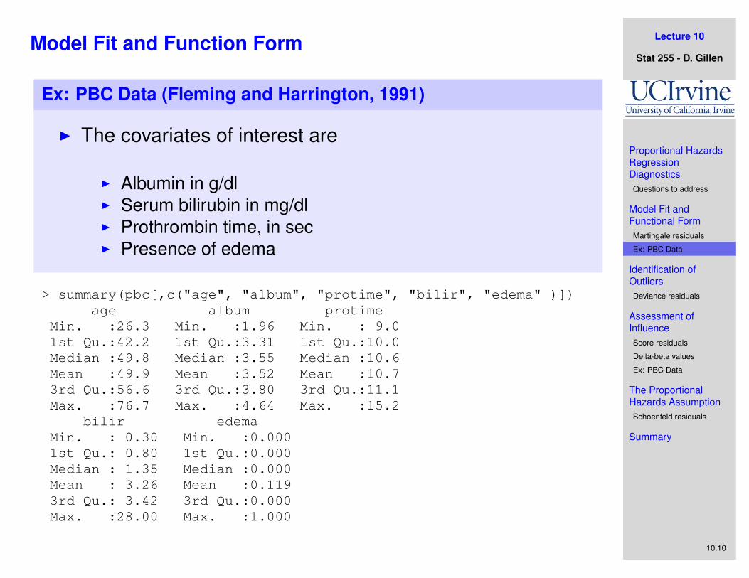
Ex: PBC Data (Fleming and Harrington, 1991)
I The covariates of interest are
I Albumin in g/dlI Serum bilirubin in mg/dlI Prothrombin time, in secI Presence of edema
> summary(pbc[,c("age", "album", "protime", "bilir", "edema" )])age album protime
Min. :26.3 Min. :1.96 Min. : 9.01st Qu.:42.2 1st Qu.:3.31 1st Qu.:10.0Median :49.8 Median :3.55 Median :10.6Mean :49.9 Mean :3.52 Mean :10.73rd Qu.:56.6 3rd Qu.:3.80 3rd Qu.:11.1Max. :76.7 Max. :4.64 Max. :15.2
bilir edemaMin. : 0.30 Min. :0.0001st Qu.: 0.80 1st Qu.:0.000Median : 1.35 Median :0.000Mean : 3.26 Mean :0.1193rd Qu.: 3.42 3rd Qu.:0.000Max. :28.00 Max. :1.000

Lecture 10
Stat 255 - D. Gillen
Proportional HazardsRegressionDiagnosticsQuestions to address
Model Fit andFunctional FormMartingale residuals
Ex: PBC Data
Identification ofOutliersDeviance residuals
Assessment ofInfluenceScore residuals
Delta-beta values
Ex: PBC Data
The ProportionalHazards AssumptionSchoenfeld residuals
Summary
10.11
Model Fit and Function Form
Ex: PBC Data (Fleming and Harrington, 1991)
I We will consider albumin, and prothrombin time on the logscale and consider doing so for bilirubin
I The starting model is one without bilirubin
> ##> ##### Fit model without bilirubin> ##> fit <- coxph( Surv(time,death) ~ age + log(album) + log(protime)
+ edema, data=pbc )> summary(fit)Call:
coef exp(coef) se(coef) z Pr(>|z|)age 0.02764 1.02802 0.00961 2.88 0.004 **log(album) -4.02771 0.01782 0.65717 -6.13 8.8e-10 ***log(protime) 5.99803 402.63670 1.04634 5.73 9.9e-09 ***edema 0.56680 1.76262 0.23396 2.42 0.015 *
exp(coef) exp(-coef) lower .95 upper .95age 1.0280 0.97274 1.00885 1.05e+00log(album) 0.0178 56.13238 0.00491 6.46e-02log(protime) 402.6367 0.00248 51.79220 3.13e+03edema 1.7626 0.56734 1.11432 2.79e+00

Lecture 10
Stat 255 - D. Gillen
Proportional HazardsRegressionDiagnosticsQuestions to address
Model Fit andFunctional FormMartingale residuals
Ex: PBC Data
Identification ofOutliersDeviance residuals
Assessment ofInfluenceScore residuals
Delta-beta values
Ex: PBC Data
The ProportionalHazards AssumptionSchoenfeld residuals
Summary
10.12
Model Fit and Function Form
Ex: PBC Data (Fleming and Harrington, 1991)
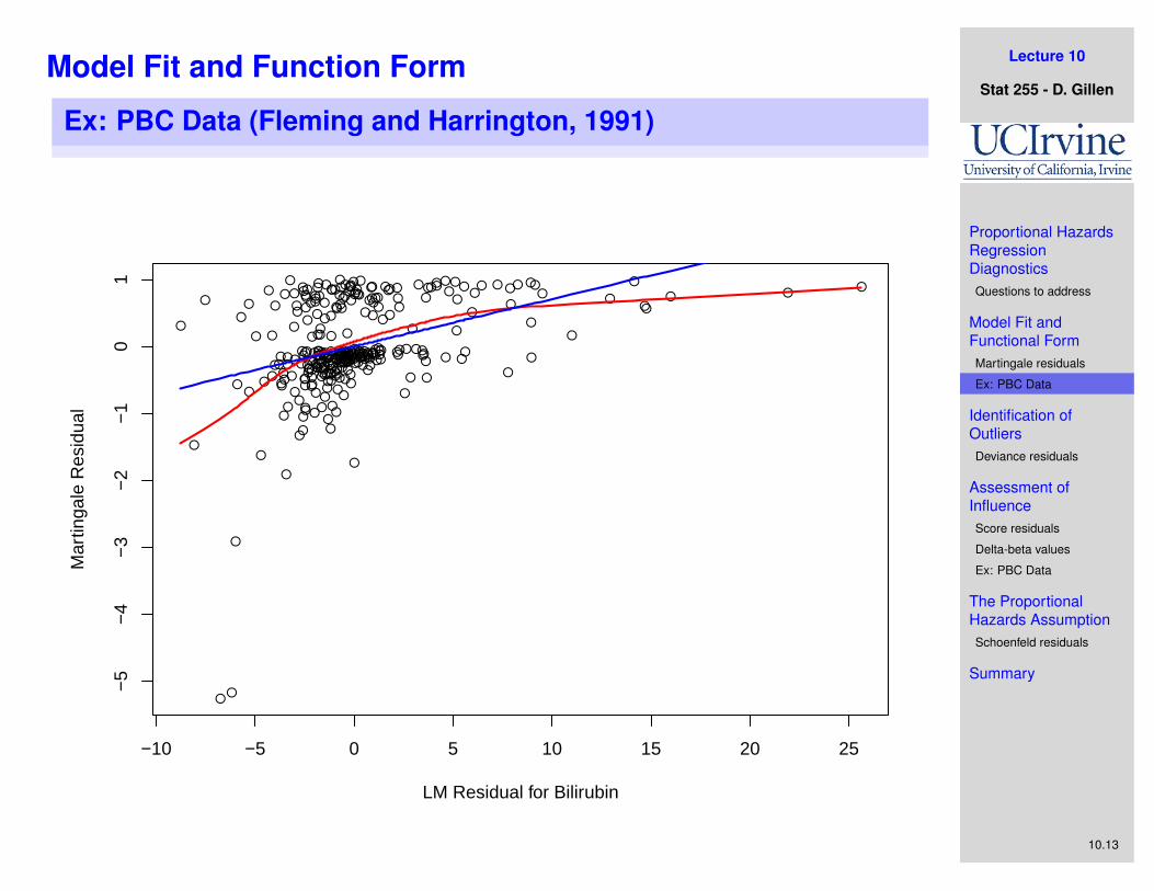
I Now, what is the correct functional form for bilirubin in thecontext of this model (that is, for predicting mortality risk,adjusting for the other covariates)?
I Martingale residual plot for bilirubin:
I need to adjust for other covariatesI use a smootherI include regression line
> mresids <- residuals( fit, type="martingale" )> lmfit <- lm( bilir ~ age + log(album) + log(protime) + edema,
data=pbc )> rbili <- lmfit$resid> ord <- order( rbili )> mresids <- mresids[ ord ]> rbili <- rbili[ ord ]> plot( rbili, mresids )> lines( smooth.spline( rbili, mresids, df=6 ), col="red", lwd=2 )> lines( rbili, fitted(lm( mresids ~ rbili )), col="blue", lwd=2 )
Lecture 10
Stat 255 - D. Gillen
Proportional HazardsRegressionDiagnosticsQuestions to address
Model Fit andFunctional FormMartingale residuals
Ex: PBC Data
Identification ofOutliersDeviance residuals
Assessment ofInfluenceScore residuals
Delta-beta values
Ex: PBC Data
The ProportionalHazards AssumptionSchoenfeld residuals
Summary
10.13
Model Fit and Function Form
Ex: PBC Data (Fleming and Harrington, 1991)
●
●
●
●●
●
●
●●
●
●
●
●
●
●
●●
●
●●
●●●
●
●
●
●
●●
●
●
●
●
●
●
●
●●
●
●
●●
●
●
●
●
●
●●●
●
●
●
●
●●
●
●
●
●●●●
●
●
●
●●
●
●
●
●
●
●●
●
●
●
●
●
●
●
●●
●
●
●
●
●
●●
●●
●●
●
●
●
●●●
●
●●
●
●
●
●
●
●
●
●
●
●
●●●
●
●
●●●●
●
●
●
●
●
●●
●●
●
●●●
●
●
●●
●
●
●
●
●●
●
●●●●
●
●
●
●
●●●
●
●
●
●●●
●
●
●●
●
●●
●
●●●
●
●
●
●●●●
●
●●
●●●●
●●
●●
●
●
●●
●
●
●●
●
●●
●
●
●●
●
●●
●●
●
●
●●●●●●
●
●●●●●●
●
●●
●
●●
●
●●
●●●
●
●●
●
●●
●
●
●
●
●
●●●●
●
●●
●
●
●
●●
●
●
●
●
●
●
●
●
●
●●●●
●
●
●●●●●
●
●●
●
●
●
●
●
●
●● ●
●
●
●
● ●
●
●
●●
●
●
●
●●● ●
●
−10 −5 0 5 10 15 20 25
−5
−4
−3
−2
−1
01
LM Residual for Bilirubin
Mar
tinga
le R
esid
ual

Lecture 10
Stat 255 - D. Gillen
Proportional HazardsRegressionDiagnosticsQuestions to address
Model Fit andFunctional FormMartingale residuals
Ex: PBC Data
Identification ofOutliersDeviance residuals
Assessment ofInfluenceScore residuals
Delta-beta values
Ex: PBC Data
The ProportionalHazards AssumptionSchoenfeld residuals
Summary
10.14
Model Fit and Function Form
Ex: PBC Data (Fleming and Harrington, 1991)
I Now, let’s consider a log-transformation for biliruibin
> lmfit <- lm( log(bilir) ~ age + log(album) + log(protime) + edema,data=pbc )
> rlogbili <- lmfit$resid> ord <- order( rlogbili )> mresids <- mresids[ ord ]> rlogbili <- rlogbili[ ord ]> plot( rlogbili, mresids )> lines( smooth.spline( rlogbili, mresids, df=6 ), col="red", lwd=2 )> lines(rlogbili, fitted(lm( mresids ~ rlogbili )), col="blue", lwd=2)

Lecture 10
Stat 255 - D. Gillen
Proportional HazardsRegressionDiagnosticsQuestions to address
Model Fit andFunctional FormMartingale residuals
Ex: PBC Data
Identification ofOutliersDeviance residuals
Assessment ofInfluenceScore residuals
Delta-beta values
Ex: PBC Data
The ProportionalHazards AssumptionSchoenfeld residuals
Summary
10.15
Model Fit and Function Form
Ex: PBC Data (Fleming and Harrington, 1991)
●
●
●
●● ●
●
●●
●
●
●
●
●●
●
●●
●●
●
●
●
●
●
●
●
●
●
●
●●●●
●
●
●●
●
●
●
●
●●
●
●●●
●
●●
●
●
●●●
●●
●●●
●
●
●
●●●●
●●●
●
●
●
●●
●●
●●●
●●●
●
●●
●●●●●
●
●
●
●
●
●●
●
●
●
●
●
●
●
●●
●
●
●
●
●
●
●
●
●●
●
●
●
●
●
●
●
●
●
●
●
●
●
●
●●
●
●
●●
●
●●●
●
●
●
●
●●
●●●
●
●
●
●
●
●
●
●
●
●
●
●
●
●●●
●●
●
●
●
●
●
●●
●
●●●●
●
●
●
●
●●●
●
●●●
●
●●
●
●
●
●
●
●
●●
●●●
●
●
●
●●●
●
●●
●
●
●
●
●
●●
●
●
●
●
●
●
●
●
●
●●●●
●
●
●●
●
●●
●
●
●
●
●●●
●
●●
●
●
●
●●
●
●●
●
●●
●
●●
●●●
●
●
●
●●●
●
●
●
●
●
●●●
●
●
●
●
●
●
●
●●
●
●
●
●
●
●
●
●
●
●
●
●
●●
●
●●
●
●
●
−2 −1 0 1 2 3
−5
−4
−3
−2
−1
01
LM Residual for Log−Bilirubin
Mar
tinga
le R
esid
ual

Lecture 10
Stat 255 - D. Gillen
Proportional HazardsRegressionDiagnosticsQuestions to address
Model Fit andFunctional FormMartingale residuals
Ex: PBC Data
Identification ofOutliersDeviance residuals
Assessment ofInfluenceScore residuals
Delta-beta values
Ex: PBC Data
The ProportionalHazards AssumptionSchoenfeld residuals
Summary
10.16
Model Fit and Function Form
Ex: PBC Data (Fleming and Harrington, 1991)
I Conclusion: In the context of this model, with the other 4covariates, the effect of log(bilirubin) on the log mortalityhazard is approximately linear
Lecture 10
Stat 255 - D. Gillen
Proportional HazardsRegressionDiagnosticsQuestions to address
Model Fit andFunctional FormMartingale residuals
Ex: PBC Data
Identification ofOutliersDeviance residuals
Assessment ofInfluenceScore residuals
Delta-beta values
Ex: PBC Data
The ProportionalHazards AssumptionSchoenfeld residuals
Summary
10.17
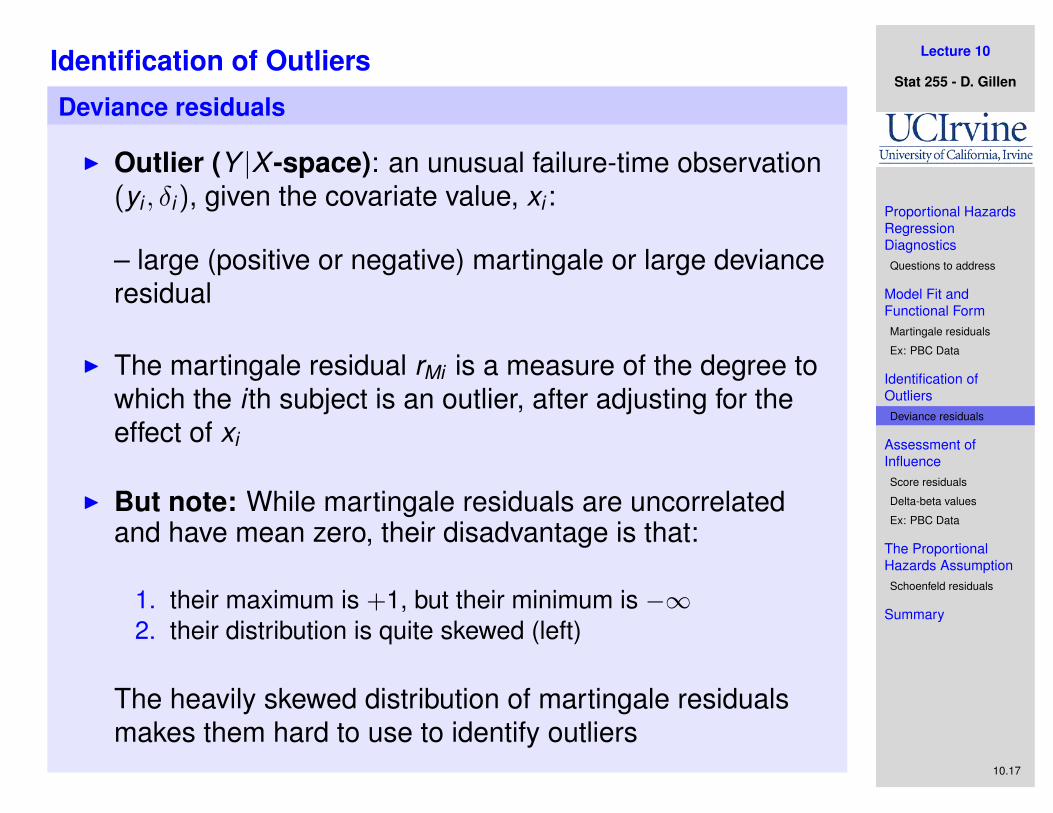
Identification of Outliers
Deviance residuals
I Outlier (Y |X -space): an unusual failure-time observation(yi , δi ), given the covariate value, xi :
– large (positive or negative) martingale or large devianceresidual
I The martingale residual rMi is a measure of the degree towhich the i th subject is an outlier, after adjusting for theeffect of xi
I But note: While martingale residuals are uncorrelatedand have mean zero, their disadvantage is that:
1. their maximum is +1, but their minimum is −∞2. their distribution is quite skewed (left)
The heavily skewed distribution of martingale residualsmakes them hard to use to identify outliers

Lecture 10
Stat 255 - D. Gillen
Proportional HazardsRegressionDiagnosticsQuestions to address
Model Fit andFunctional FormMartingale residuals
Ex: PBC Data
Identification ofOutliersDeviance residuals
Assessment ofInfluenceScore residuals
Delta-beta values
Ex: PBC Data
The ProportionalHazards AssumptionSchoenfeld residuals
Summary
10.18
Identification of Outliers
Deviance residuals
I For this, we have deviance residuals:
rDi = sign(rMi ) [−2 {rMi + δi log(δi − rMi )}]1/2
I Why are they called deviance residuals?
I From GLMs, the deviance of a model is defined as
dev(model) = 2[log L(saturated model)− log L(model)]
where a “saturated model” is one that perfectly reproducesthe data
I Deviance residuals are created in the same spirit. Namely,
dev(model) =∑
i
r 2Di

Lecture 10
Stat 255 - D. Gillen
Proportional HazardsRegressionDiagnosticsQuestions to address
Model Fit andFunctional FormMartingale residuals
Ex: PBC Data
Identification ofOutliersDeviance residuals
Assessment ofInfluenceScore residuals
Delta-beta values
Ex: PBC Data
The ProportionalHazards AssumptionSchoenfeld residuals
Summary
10.19
Identification of Outliers
Behavior of deviance residuals
I rDi has the same sign as rMi :
I The quantity inside the [ ]’s is positive (so we can take thesquare root), while sign(·) assures that the devianceresidual has the same sign as the martingale residual
I What happens when . . .
I rMi ≈ 0?
I rMi is close to 1
I rMi is large and negative

Lecture 10
Stat 255 - D. Gillen
Proportional HazardsRegressionDiagnosticsQuestions to address
Model Fit andFunctional FormMartingale residuals
Ex: PBC Data
Identification ofOutliersDeviance residuals
Assessment ofInfluenceScore residuals
Delta-beta values
Ex: PBC Data
The ProportionalHazards AssumptionSchoenfeld residuals
Summary
10.20
Identification of Outliers
Behavior of deviance residuals
I Compared to rMi , rDi has a shorter left and a longer righttail−→ rDi is more symmetrical around zero
I The distribution of the deviance residual is betterapproximated by a Gaussian distribution than is thedistribution of the martingale residuals
I Because they are approximately normally distributed, youcan think of outliers as values outside of the range of(−3,+3) or even (−2.5,2.5)

Lecture 10
Stat 255 - D. Gillen
Proportional HazardsRegressionDiagnosticsQuestions to address
Model Fit andFunctional FormMartingale residuals
Ex: PBC Data
Identification ofOutliersDeviance residuals
Assessment ofInfluenceScore residuals
Delta-beta values
Ex: PBC Data
The ProportionalHazards AssumptionSchoenfeld residuals
Summary
10.21
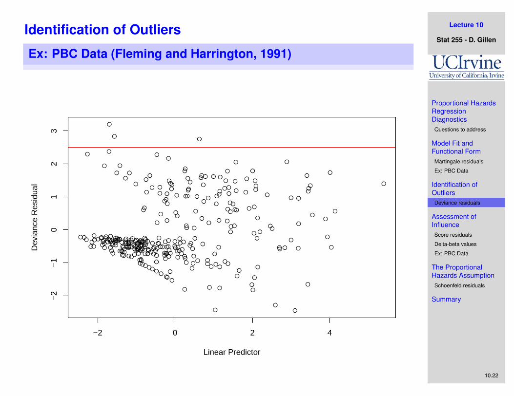
Identification of Outliers
Ex: PBC Data (Fleming and Harrington, 1991)
I Goal: Determine if there are any outliers in the model withall covariates, plus log(bilirubin)
I Approach: Plot residuals versus the “risk scores” β̂T xi :
I Start by fitting the model with log(bilirubin), then obtainlinear predictor estimates and the deviance residuals...
> ##> ##### Consider outliers (in the X-space)> fit <- coxph( Surv(time,death) ~ age + log(album) + log(protime) +
edema + log(bilir), data=pbc )> summary(fit)
exp(coef) exp(-coef) lower .95 upper .95age 1.0415 0.9602 1.0226 1.061log(album) 0.0441 22.6812 0.0109 0.178log(protime) 42.5586 0.0235 4.7547 380.937edema 1.5055 0.6643 0.9450 2.398log(bilir) 2.4623 0.4061 2.0257 2.993
> dresids <- residuals( fit, type="deviance" )> lp <- predict( fit, type="lp" )> plot(lp, dresids, xlab="Linear Predictor", ylab="Deviance Residual")
Lecture 10
Stat 255 - D. Gillen
Proportional HazardsRegressionDiagnosticsQuestions to address
Model Fit andFunctional FormMartingale residuals
Ex: PBC Data
Identification ofOutliersDeviance residuals
Assessment ofInfluenceScore residuals
Delta-beta values
Ex: PBC Data
The ProportionalHazards AssumptionSchoenfeld residuals
Summary
10.22
Identification of Outliers
Ex: PBC Data (Fleming and Harrington, 1991)
●
●
●
●
●
●
●
●
●
●
●
●
●
●●
●
●
●
●
●
●
●
●●
●
●
●
●
●
●
●
●
●
●
●
●
●
●
●
●
●
●●
●
●
●
●
●
●
●
●
●
●
●
●
●
●
●
●
●
●
●
●
●
●
●
●
●●●
●
●
●
●
●
●
●
●
●
●
●
●
●
●
●●
●
●
●
●●
●
●
● ●
●
●
●
●
●
●●
●
●
●
●
●
●
●
●
●
●
●
●
●
●
●●
●
●
●
●
●
● ●
●
●●
●
●
●
●
●
●●
●●
●
●●●
●
●
●
●
●
●
●
●
●
●
●
●
●
●
●
●
●
●
●●
●
●
●
●
●
●
●
●
●
●
●●
●●
●
●●●
●●
●
●
●
●
●
●
●●
●
●
●
●
●
●
●
●●
●
●
●●
●
●
●
●
●
●
●
● ●●●
●
●
●
●
●●
●
●
●
●●● ●
●
●
●
●
●●●●
●
●
●
●
●
● ●
●
●
●
● ●
●●
●
●●
●
●
●●● ●●
●
●
●●
●
●
●
●
●
●
●
●●
●
●●
● ●●
●
●●
●
● ●●●
●
●
●
●
●●
●
●
●
●● ●●●
●
●●
●
●
●●
● ●●
●● ●
−2 0 2 4
−2
−1
01
23
Linear Predictor
Dev
ianc
e R
esid
ual

Lecture 10
Stat 255 - D. Gillen
Proportional HazardsRegressionDiagnosticsQuestions to address
Model Fit andFunctional FormMartingale residuals
Ex: PBC Data
Identification ofOutliersDeviance residuals
Assessment ofInfluenceScore residuals
Delta-beta values
Ex: PBC Data
The ProportionalHazards AssumptionSchoenfeld residuals
Summary
10.23
Identification of Outliers
Ex: PBC Data (Fleming and Harrington, 1991)
I Let’s investigate the three outliers...
> summary(pbc[,c("age", "album", "protime", "bilir", "edema" )])age album protime bilir
Min. :26.3 Min. :1.96 Min. : 9.0 Min. : 0.301st Qu.:42.2 1st Qu.:3.31 1st Qu.:10.0 1st Qu.: 0.80Median :49.8 Median :3.55 Median :10.6 Median : 1.35Mean :49.9 Mean :3.52 Mean :10.7 Mean : 3.263rd Qu.:56.6 3rd Qu.:3.80 3rd Qu.:11.1 3rd Qu.: 3.42Max. :76.7 Max. :4.64 Max. :15.2 Max. :28.00
edemaMin. :0.0001st Qu.:0.000Median :0.000Mean :0.1193rd Qu.:0.000Max. :1.000
> cbind( dresids,pbc[,c("time", "death", "age", "album", "protime","bilir", "edema" )] )[ abs(dresids) >= 2.5, ]
dresids time death age album protime bilir edema87 3.2003 198 1 37.279 4.40 10.7 1.1 0103 2.7535 110 1 48.964 3.67 11.1 2.5 1119 2.8327 515 1 54.256 3.83 9.5 0.6 0
Lecture 10
Stat 255 - D. Gillen
Proportional HazardsRegressionDiagnosticsQuestions to address
Model Fit andFunctional FormMartingale residuals
Ex: PBC Data
Identification ofOutliersDeviance residuals
Assessment ofInfluenceScore residuals
Delta-beta values
Ex: PBC Data
The ProportionalHazards AssumptionSchoenfeld residuals
Summary
10.24
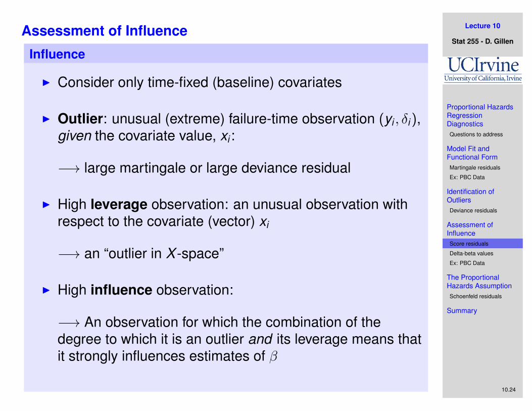
Assessment of Influence
Influence
I Consider only time-fixed (baseline) covariates
I Outlier: unusual (extreme) failure-time observation (yi , δi ),given the covariate value, xi :
−→ large martingale or large deviance residual
I High leverage observation: an unusual observation withrespect to the covariate (vector) xi
−→ an “outlier in X -space”
I High influence observation:
−→ An observation for which the combination of thedegree to which it is an outlier and its leverage means thatit strongly influences estimates of β

Lecture 10
Stat 255 - D. Gillen
Proportional HazardsRegressionDiagnosticsQuestions to address
Model Fit andFunctional FormMartingale residuals
Ex: PBC Data
Identification ofOutliersDeviance residuals
Assessment ofInfluenceScore residuals
Delta-beta values
Ex: PBC Data
The ProportionalHazards AssumptionSchoenfeld residuals
Summary
10.25
Assessment of Influence
How influence is operationalized
I Recall that the martingale residual is . . .
rMi = δi − Λ̂i (Yi | xi )
I The martingale residual rMi is a measure of the degree towhich the i th subject is an outlier, after adjusting for theeffect of xi . . . and note that the martingale residual couldbe rewritten as
rMi =∑
t(k)≤Yi
{δi (t(k))− eβ̂
T xi [Λ̂0(t(k))− Λ̂0(t(k−1))]}
rMi =∑
t(k)≤Yi
{δi (t(k))− eβ̂
T xi d Λ̂0(t(k))}
rMi =∑
t(k)≤Yi
rMik
Lecture 10
Stat 255 - D. Gillen
Proportional HazardsRegressionDiagnosticsQuestions to address
Model Fit andFunctional FormMartingale residuals
Ex: PBC Data
Identification ofOutliersDeviance residuals
Assessment ofInfluenceScore residuals
Delta-beta values
Ex: PBC Data
The ProportionalHazards AssumptionSchoenfeld residuals
Summary
10.26
Assessment of Influence
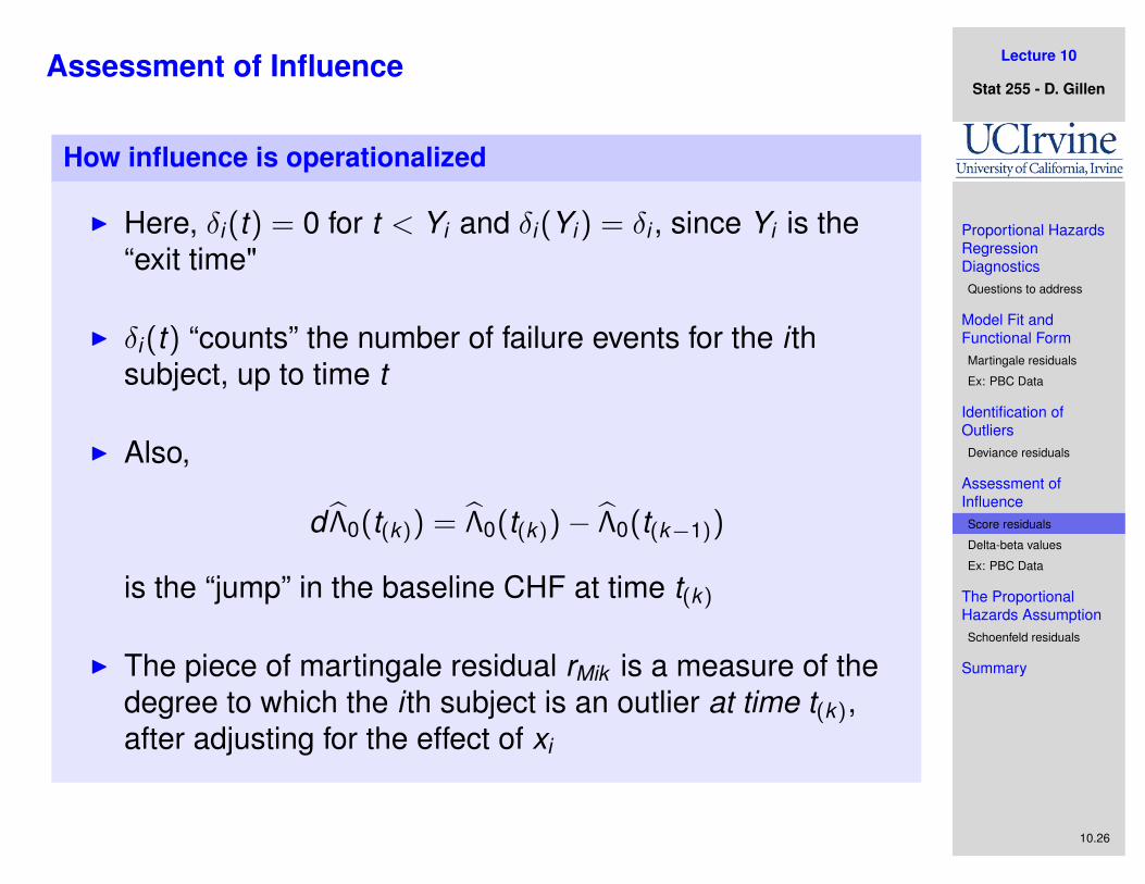
How influence is operationalized
I Here, δi (t) = 0 for t < Yi and δi (Yi ) = δi , since Yi is the“exit time"
I δi (t) “counts” the number of failure events for the i thsubject, up to time t
I Also,
d Λ̂0(t(k)) = Λ̂0(t(k))− Λ̂0(t(k−1))
is the “jump” in the baseline CHF at time t(k)
I The piece of martingale residual rMik is a measure of thedegree to which the i th subject is an outlier at time t(k),after adjusting for the effect of xi
Lecture 10
Stat 255 - D. Gillen
Proportional HazardsRegressionDiagnosticsQuestions to address
Model Fit andFunctional FormMartingale residuals
Ex: PBC Data
Identification ofOutliersDeviance residuals
Assessment ofInfluenceScore residuals
Delta-beta values
Ex: PBC Data
The ProportionalHazards AssumptionSchoenfeld residuals
Summary
10.27
Assessment of Influence
How influence is operationalized
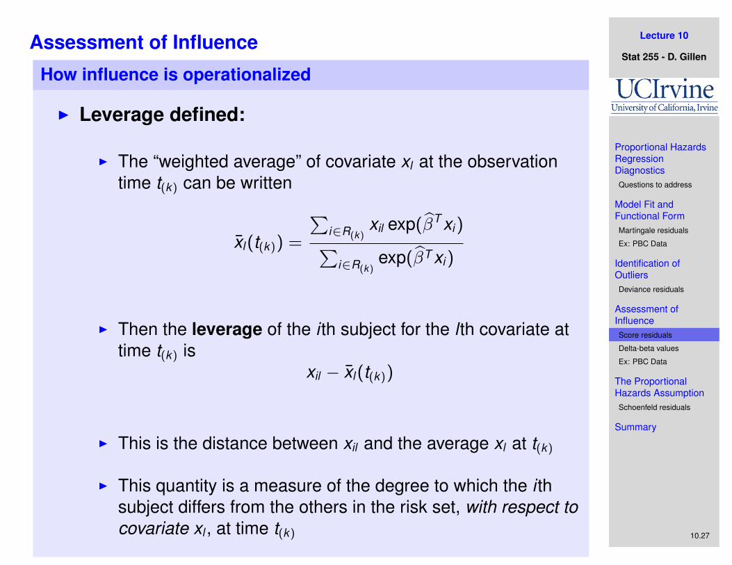
I Leverage defined:
I The “weighted average” of covariate xl at the observationtime t(k) can be written
x̄l (t(k)) =
∑i∈R(k)
xil exp(β̂T xi )∑i∈R(k)
exp(β̂T xi )
I Then the leverage of the i th subject for the l th covariate attime t(k) is
xil − x̄l (t(k))
I This is the distance between xil and the average xl at t(k)
I This quantity is a measure of the degree to which the i thsubject differs from the others in the risk set, with respect tocovariate xl , at time t(k)

Lecture 10
Stat 255 - D. Gillen
Proportional HazardsRegressionDiagnosticsQuestions to address
Model Fit andFunctional FormMartingale residuals
Ex: PBC Data
Identification ofOutliersDeviance residuals
Assessment ofInfluenceScore residuals
Delta-beta values
Ex: PBC Data
The ProportionalHazards AssumptionSchoenfeld residuals
Summary
10.28
Assessment of Influence
How influence is operationalized – Score residuals
I Influence is then operationalized as the integral ofleverage times the martingale residuals:
rSli =∑
t(k)≤Yi
(xil − x̄l (t(k)))︸ ︷︷ ︸leverage
×{δi (t(k))− eβ̂
T xi d Λ̂0(t(k))}
︸ ︷︷ ︸Martingale residual
I Qualitatively, influence is the product of leverage andoutlying tendency
I The quantities rSli are called score residuals
I There is one set of score residuals for each covariate xil inthe model, l = 1, . . . , p
I Large values of rSli imply large influence of the i th subjecton the estimate of βl , the coefficient for xl
I Obtain in R with residuals(fit, type="score")
Lecture 10
Stat 255 - D. Gillen
Proportional HazardsRegressionDiagnosticsQuestions to address
Model Fit andFunctional FormMartingale residuals
Ex: PBC Data
Identification ofOutliersDeviance residuals
Assessment ofInfluenceScore residuals
Delta-beta values
Ex: PBC Data
The ProportionalHazards AssumptionSchoenfeld residuals
Summary
10.29
Assessment of Influence
How influence is operationalized – Delta-beta values
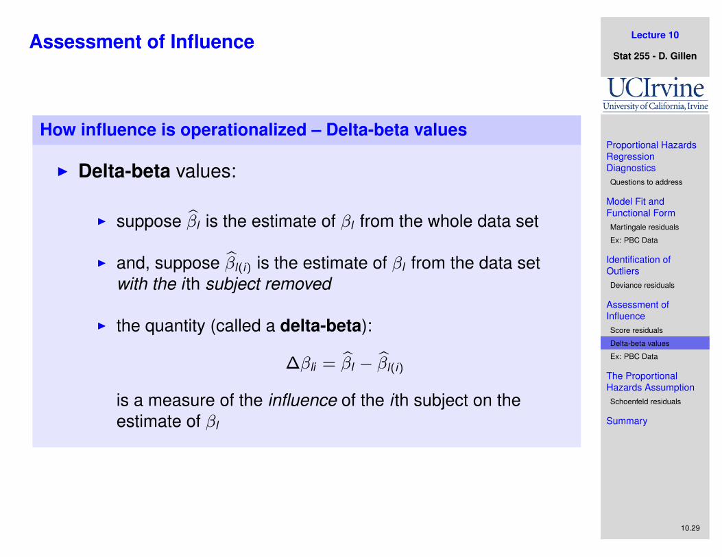
I Delta-beta values:
I suppose β̂l is the estimate of βl from the whole data set
I and, suppose β̂l(i) is the estimate of βl from the data setwith the i th subject removed
I the quantity (called a delta-beta):
∆βli = β̂l − β̂l(i)
is a measure of the influence of the i th subject on theestimate of βl

Lecture 10
Stat 255 - D. Gillen
Proportional HazardsRegressionDiagnosticsQuestions to address
Model Fit andFunctional FormMartingale residuals
Ex: PBC Data
Identification ofOutliersDeviance residuals
Assessment ofInfluenceScore residuals
Delta-beta values
Ex: PBC Data
The ProportionalHazards AssumptionSchoenfeld residuals
Summary
10.30
Assessment of Influence
How influence is operationalized – Delta-beta values
I As it turns out, ∆βli can be approximated by:
∆βli = β̂l − β̂l(i) ≈ V̂l · rSi
where rSi is the vector
rSi = (rS1i , . . . , rSpi )
of score residuals for the i th subject (across allcovariates)and V̂l is the l th row of the estimatedvariance-covariance matrix of β̂
I Each subject i has one ∆β value for each covariate in themodel

Lecture 10
Stat 255 - D. Gillen
Proportional HazardsRegressionDiagnosticsQuestions to address
Model Fit andFunctional FormMartingale residuals
Ex: PBC Data
Identification ofOutliersDeviance residuals
Assessment ofInfluenceScore residuals
Delta-beta values
Ex: PBC Data
The ProportionalHazards AssumptionSchoenfeld residuals
Summary
10.31
Assessment of Influence
Ex: PBC Data (Fleming and Harrington, 1991
I Goal: Investigate the influence of observations on thecoefficients of in the 5-variable model which we have beeninvestigating
> ##> ##### A look at delta-betas for influential points> ##> dfbeta <- residuals( fit, type="dfbeta" )> colnames( dfbeta ) <- names(fit$coef)> summary( dfbeta )
age log(album) log(protime)Min. :-4.49e-03 Min. :-1.96e-01 Min. :-4.43e-011st Qu.:-6.50e-05 1st Qu.:-1.07e-02 1st Qu.:-1.15e-02Median : 4.75e-05 Median :-1.67e-03 Median : 3.25e-03Mean : 1.72e-18 Mean :-4.58e-17 Mean : 1.10e-163rd Qu.: 1.86e-04 3rd Qu.: 6.30e-03 3rd Qu.: 1.82e-02Max. : 2.28e-03 Max. : 1.95e-01 Max. : 3.09e-01
edema log(bilir)Min. :-1.08e-01 Min. :-6.55e-021st Qu.:-7.98e-04 1st Qu.:-4.07e-04Median : 4.52e-05 Median : 8.29e-04Mean :-7.09e-16 Mean : 1.65e-173rd Qu.: 1.72e-03 3rd Qu.: 2.10e-03Max. : 5.48e-02 Max. : 2.58e-02
Lecture 10
Stat 255 - D. Gillen
Proportional HazardsRegressionDiagnosticsQuestions to address
Model Fit andFunctional FormMartingale residuals
Ex: PBC Data
Identification ofOutliersDeviance residuals
Assessment ofInfluenceScore residuals
Delta-beta values
Ex: PBC Data
The ProportionalHazards AssumptionSchoenfeld residuals
Summary
10.32
Assessment of Influence
Ex: PBC Data (Fleming and Harrington, 1991
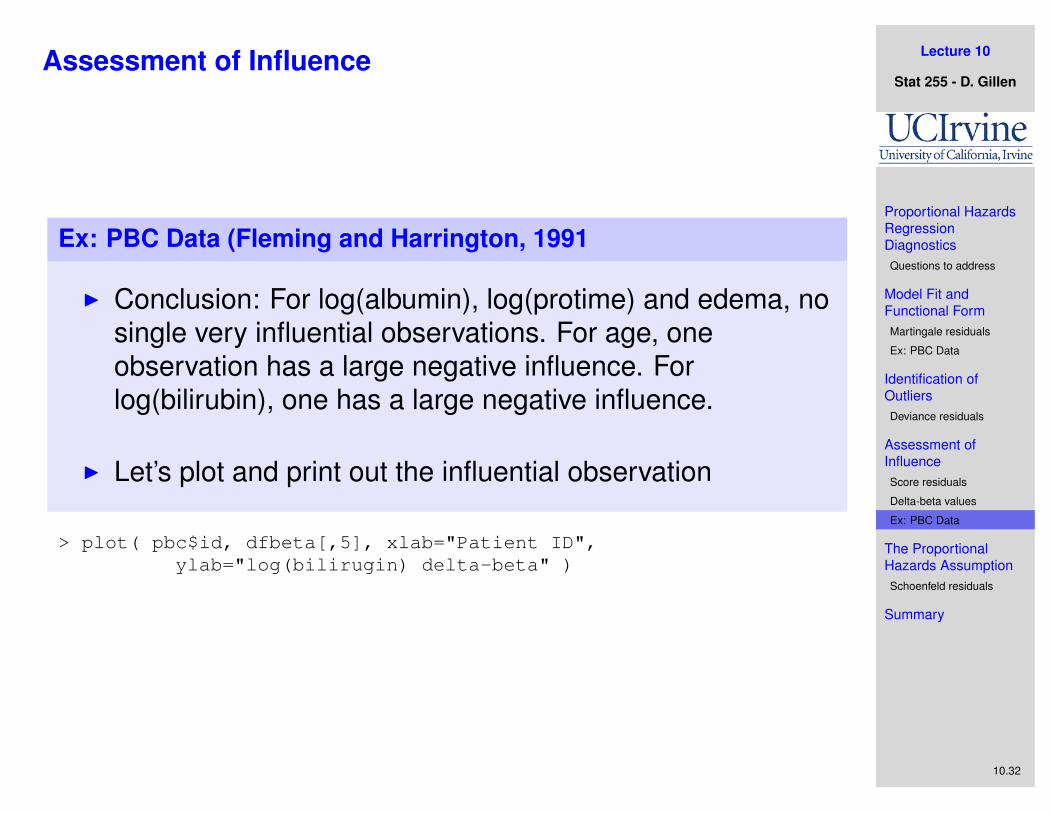
I Conclusion: For log(albumin), log(protime) and edema, nosingle very influential observations. For age, oneobservation has a large negative influence. Forlog(bilirubin), one has a large negative influence.
I Let’s plot and print out the influential observation
> plot( pbc$id, dfbeta[,5], xlab="Patient ID",ylab="log(bilirugin) delta-beta" )

Lecture 10
Stat 255 - D. Gillen
Proportional HazardsRegressionDiagnosticsQuestions to address
Model Fit andFunctional FormMartingale residuals
Ex: PBC Data
Identification ofOutliersDeviance residuals
Assessment ofInfluenceScore residuals
Delta-beta values
Ex: PBC Data
The ProportionalHazards AssumptionSchoenfeld residuals
Summary
10.33
Assessment of Influence
Ex: PBC Data (Fleming and Harrington, 1991
●
●
●
●
●
●
●
●
●
●●
●
●
●
●●
●
●●●●
●
●●●
●●
●●
●
●●●
●●●
●
●
●
●●
●●●●●
●●
●
●●●
●
●
●
●
●
●
●
●
●
●
●
●●●●●
●
●
●
●●
●
●
●
●
●●●
●
●
●
●●●
●
●●●
●
●
●
●
●
●
●
●●
●
●●
●
●●●●
●
●●●
●●●●
●
●●
●
●
●
●●●●
●
●
●
●●
●
●
●
●●●●
●
●●●
●●
●●●
●●
●●●●●
●
●
●
●●●●●
●
●
●●
●●
●
●
●●●●●●●●●●
●
●●●
●
●●
●●●●●●
●
●●
●
●●●●
●●●
●
●●
●●●●●●●
●
●●
●
●●
●●
●●●●●●●
●●
●
●●●
●
●●●
●
●●●●
●
●●●●●●●●
●
●●●●●●
●
●●●●●●●
●●●●●●●●●●●●●
●●●●●●
●●
●●●
●
●●
●●●●●
●
●●●●●●●●
●●●●
0 50 100 150 200 250 300
−0.
06−
0.04
−0.
020.
000.
02
Patient ID
log(
bilir
ugin
) de
lta−
beta
> pbc[ dfbeta[,5] < -.04, ]age album alkph ascites bilir chol edema edematx hepat
81 63.264 3.65 1218 0 14.4 448 0 0 1time plate protime sex sgot spiders stage death treat trigl
81 2540 385 11.7 1 60.45 1 4 1 1 318ucopp rand id
81 34 1 81

Lecture 10
Stat 255 - D. Gillen
Proportional HazardsRegressionDiagnosticsQuestions to address
Model Fit andFunctional FormMartingale residuals
Ex: PBC Data
Identification ofOutliersDeviance residuals
Assessment ofInfluenceScore residuals
Delta-beta values
Ex: PBC Data
The ProportionalHazards AssumptionSchoenfeld residuals
Summary
10.34
Assessment of Influence
Ex: PBC Data (Fleming and Harrington, 1991
I Conclusion: Subject 81 is older and has a high serumbilirubin (2 sd above mean on log scale). Bilirubin is animportant predictor of high risk, yet subject is in the 40th(or so) percentile of survival times
I Recommendation: If interest is on assessing the effect ofbilirubin, might do a sensitivity analysis (ie. present resultswith this case and without)
I Important: Unless it is very, very clear that there is somesort of data entry error causing a problem, it is generallynever a good idea to permanently remove an observationfrom your data!
Lecture 10
Stat 255 - D. Gillen
Proportional HazardsRegressionDiagnosticsQuestions to address
Model Fit andFunctional FormMartingale residuals
Ex: PBC Data
Identification ofOutliersDeviance residuals
Assessment ofInfluenceScore residuals
Delta-beta values
Ex: PBC Data
The ProportionalHazards AssumptionSchoenfeld residuals
Summary
10.35
The Proportional Hazards Assumption
Schoenfeld residuals
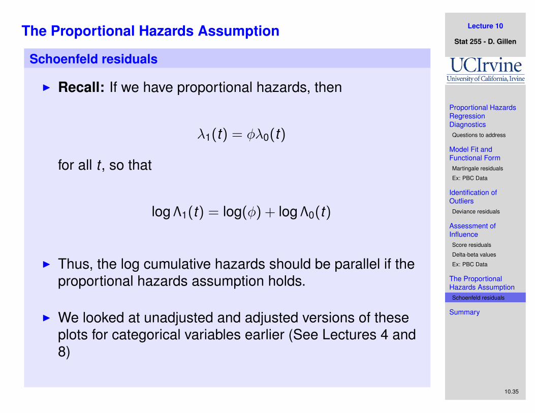
I Recall: If we have proportional hazards, then
λ1(t) = φλ0(t)
for all t , so that
log Λ1(t) = log(φ) + log Λ0(t)
I Thus, the log cumulative hazards should be parallel if theproportional hazards assumption holds.
I We looked at unadjusted and adjusted versions of theseplots for categorical variables earlier (See Lectures 4 and8)
Lecture 10
Stat 255 - D. Gillen
Proportional HazardsRegressionDiagnosticsQuestions to address
Model Fit andFunctional FormMartingale residuals
Ex: PBC Data
Identification ofOutliersDeviance residuals
Assessment ofInfluenceScore residuals
Delta-beta values
Ex: PBC Data
The ProportionalHazards AssumptionSchoenfeld residuals
Summary
10.36
The Proportional Hazards Assumption
Schoenfeld residuals
I Let’s consider whether edema exhibits a non-proportionalhazards effect
> fit <- coxph( Surv(time,death) ~ age + log(album) +log(protime) + log(bilir) + strata(edema), data=pbc )
> plot( survfit(fit), fun="cloglog", lty=1:2,+ xlab="Time from Randomization (days)",+ ylab="Log-Cumulative Hazard Function" )> legend( 50, 0, lty=1:2, legend=c("No Edema", "Edema"), bty="n" )
Lecture 10
Stat 255 - D. Gillen
Proportional HazardsRegressionDiagnosticsQuestions to address
Model Fit andFunctional FormMartingale residuals
Ex: PBC Data
Identification ofOutliersDeviance residuals
Assessment ofInfluenceScore residuals
Delta-beta values
Ex: PBC Data
The ProportionalHazards AssumptionSchoenfeld residuals
Summary
10.37
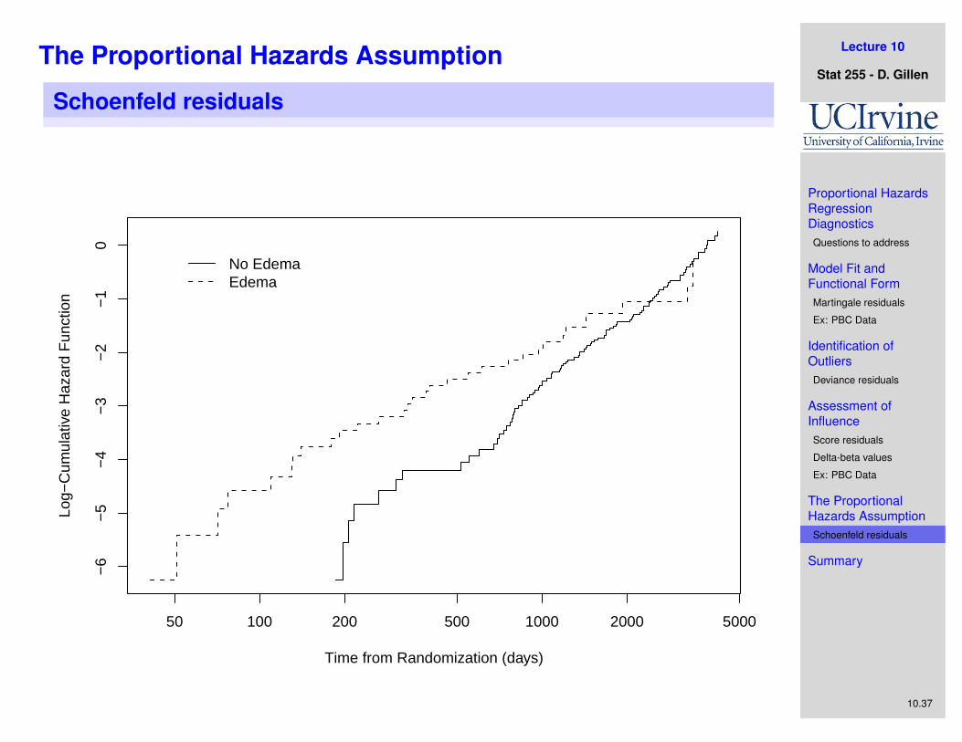
The Proportional Hazards Assumption
Schoenfeld residuals
50 100 200 500 1000 2000 5000
−6
−5
−4
−3
−2
−1
0
Time from Randomization (days)
Log−
Cum
ulat
ive
Haz
ard
Fun
ctio
n
No EdemaEdema

Lecture 10
Stat 255 - D. Gillen
Proportional HazardsRegressionDiagnosticsQuestions to address
Model Fit andFunctional FormMartingale residuals
Ex: PBC Data
Identification ofOutliersDeviance residuals
Assessment ofInfluenceScore residuals
Delta-beta values
Ex: PBC Data
The ProportionalHazards AssumptionSchoenfeld residuals
Summary
10.38
The Proportional Hazards Assumption
Schoenfeld residuals
I Clearly the log cumulative hazards are not parallel
I This suggests that the proportional hazards assumptionmay be violated, ie. The hazard ratio associated withedema may be changing with respect to time.
I We have looked at one test of this assumption using timedependent covariates. Another relies upon the Schoenfeldresiduals...
Lecture 10
Stat 255 - D. Gillen
Proportional HazardsRegressionDiagnosticsQuestions to address
Model Fit andFunctional FormMartingale residuals
Ex: PBC Data
Identification ofOutliersDeviance residuals
Assessment ofInfluenceScore residuals
Delta-beta values
Ex: PBC Data
The ProportionalHazards AssumptionSchoenfeld residuals
Summary
10.39
The Proportional Hazards Assumption
Schoenfeld residuals
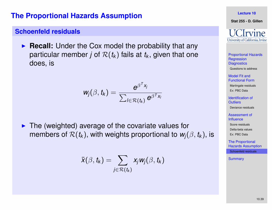
I Recall: Under the Cox model the probability that anyparticular member j of R(tk ) fails at tk , given that onedoes, is
wj (β, tk ) =eβ
T xj∑l∈R(tk ) eβT xl
I The (weighted) average of the covariate values formembers of R(tk ), with weights proportional to wj (β, tk ), is
x̄(β, tk ) =∑
j∈R(tk )
xjwj (β, tk )
Lecture 10
Stat 255 - D. Gillen
Proportional HazardsRegressionDiagnosticsQuestions to address
Model Fit andFunctional FormMartingale residuals
Ex: PBC Data
Identification ofOutliersDeviance residuals
Assessment ofInfluenceScore residuals
Delta-beta values
Ex: PBC Data
The ProportionalHazards AssumptionSchoenfeld residuals
Summary
10.40
The Proportional Hazards Assumption
Schoenfeld residuals
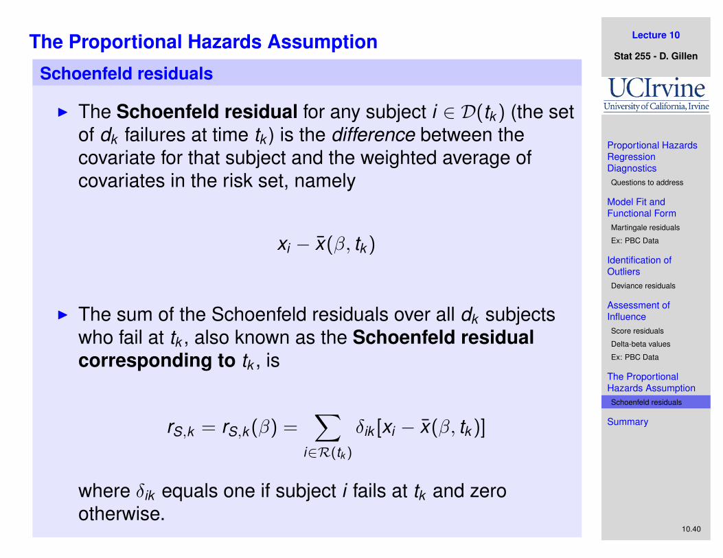
I The Schoenfeld residual for any subject i ∈ D(tk ) (the setof dk failures at time tk ) is the difference between thecovariate for that subject and the weighted average ofcovariates in the risk set, namely
xi − x̄(β, tk )
I The sum of the Schoenfeld residuals over all dk subjectswho fail at tk , also known as the Schoenfeld residualcorresponding to tk , is
rS,k = rS,k (β) =∑
i∈R(tk )
δik [xi − x̄(β, tk )]
where δik equals one if subject i fails at tk and zerootherwise.

Lecture 10
Stat 255 - D. Gillen
Proportional HazardsRegressionDiagnosticsQuestions to address
Model Fit andFunctional FormMartingale residuals
Ex: PBC Data
Identification ofOutliersDeviance residuals
Assessment ofInfluenceScore residuals
Delta-beta values
Ex: PBC Data
The ProportionalHazards AssumptionSchoenfeld residuals
Summary
10.41
The Proportional Hazards Assumption
Schoenfeld residuals
I Provided the PH model holds and β is the true regressioncoefficient, the rS,k (β) are uncorrelated and have meanzero.
I In practice the Schoenfeld residuals are calculated as
r̂S,k = rS,k (β̂)
where β̂ is the partial likelihood estimate of the regressioncoefficients.
I Schoenfeld residuals are also known as partial scoreresiduals, because their total equals the partial likelihoodscore, or estimating equation, whose solution is β̂:∑
k
rS,k (β̂) = 0

Lecture 10
Stat 255 - D. Gillen
Proportional HazardsRegressionDiagnosticsQuestions to address
Model Fit andFunctional FormMartingale residuals
Ex: PBC Data
Identification ofOutliersDeviance residuals
Assessment ofInfluenceScore residuals
Delta-beta values
Ex: PBC Data
The ProportionalHazards AssumptionSchoenfeld residuals
Summary
10.42
The Proportional Hazards Assumption
Schoenfeld residuals
I Scaled Schoefeld residuals are residuals aftermultiplication by the inverse weighted covariance matrix ofβ̂:
r∗S,k = r∗S,k (β) = V−1(β)rS,k (β)
Lecture 10
Stat 255 - D. Gillen
Proportional HazardsRegressionDiagnosticsQuestions to address
Model Fit andFunctional FormMartingale residuals
Ex: PBC Data
Identification ofOutliersDeviance residuals
Assessment ofInfluenceScore residuals
Delta-beta values
Ex: PBC Data
The ProportionalHazards AssumptionSchoenfeld residuals
Summary
10.43
The Proportional Hazards Assumption
Schoenfeld residuals
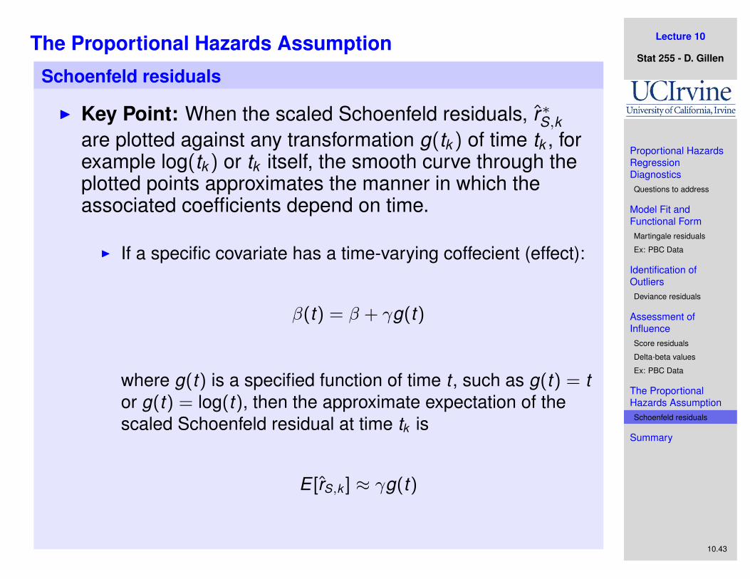
I Key Point: When the scaled Schoenfeld residuals, r̂∗S,kare plotted against any transformation g(tk ) of time tk , forexample log(tk ) or tk itself, the smooth curve through theplotted points approximates the manner in which theassociated coefficients depend on time.
I If a specific covariate has a time-varying coffecient (effect):
β(t) = β + γg(t)
where g(t) is a specified function of time t , such as g(t) = tor g(t) = log(t), then the approximate expectation of thescaled Schoenfeld residual at time tk is
E [r̂S,k ] ≈ γg(t)
Lecture 10
Stat 255 - D. Gillen
Proportional HazardsRegressionDiagnosticsQuestions to address
Model Fit andFunctional FormMartingale residuals
Ex: PBC Data
Identification ofOutliersDeviance residuals
Assessment ofInfluenceScore residuals
Delta-beta values
Ex: PBC Data
The ProportionalHazards AssumptionSchoenfeld residuals
Summary
10.44
The Proportional Hazards Assumption
Schoenfeld residuals
I This suggests:
I Plotting r̂∗S,k against g(tk ) and examining trends
I Slope of linear regression gives numerator of the scorestatistic, γ̂ for testing H0 : γ = 0 (proportionality)
I This test is implemented in R via the cox.zph() command
Lecture 10
Stat 255 - D. Gillen
Proportional HazardsRegressionDiagnosticsQuestions to address
Model Fit andFunctional FormMartingale residuals
Ex: PBC Data
Identification ofOutliersDeviance residuals
Assessment ofInfluenceScore residuals
Delta-beta values
Ex: PBC Data
The ProportionalHazards AssumptionSchoenfeld residuals
Summary
10.45
The Proportional Hazards Assumption
Schoenfeld residuals
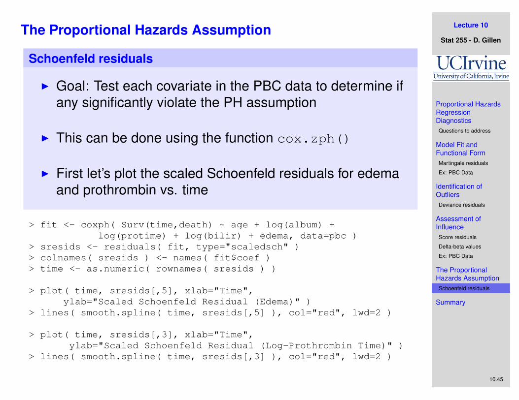
I Goal: Test each covariate in the PBC data to determine ifany significantly violate the PH assumption
I This can be done using the function cox.zph()
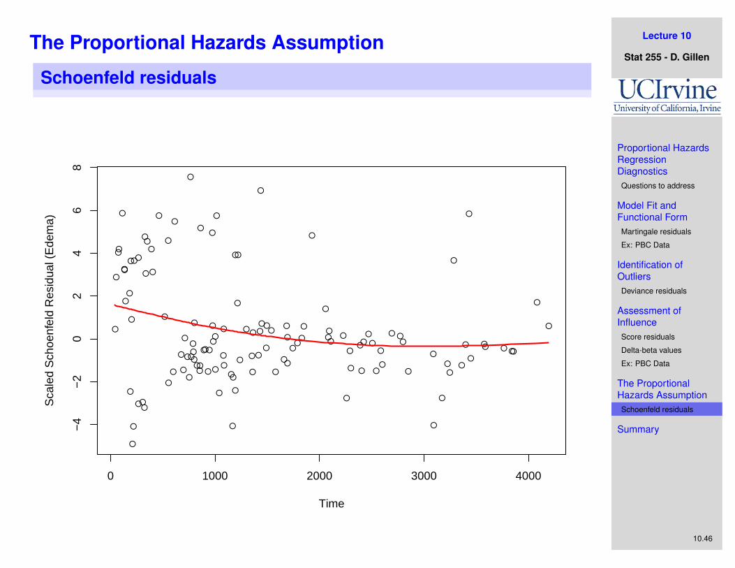
I First let’s plot the scaled Schoenfeld residuals for edemaand prothrombin vs. time
> fit <- coxph( Surv(time,death) ~ age + log(album) +log(protime) + log(bilir) + edema, data=pbc )
> sresids <- residuals( fit, type="scaledsch" )> colnames( sresids ) <- names( fit$coef )> time <- as.numeric( rownames( sresids ) )
> plot( time, sresids[,5], xlab="Time",ylab="Scaled Schoenfeld Residual (Edema)" )
> lines( smooth.spline( time, sresids[,5] ), col="red", lwd=2 )
> plot( time, sresids[,3], xlab="Time",ylab="Scaled Schoenfeld Residual (Log-Prothrombin Time)" )
> lines( smooth.spline( time, sresids[,3] ), col="red", lwd=2 )
Lecture 10
Stat 255 - D. Gillen
Proportional HazardsRegressionDiagnosticsQuestions to address
Model Fit andFunctional FormMartingale residuals
Ex: PBC Data
Identification ofOutliersDeviance residuals
Assessment ofInfluenceScore residuals
Delta-beta values
Ex: PBC Data
The ProportionalHazards AssumptionSchoenfeld residuals
Summary
10.46
The Proportional Hazards Assumption
Schoenfeld residuals
●
●
●●
●
●●
●●
●
●
●
●
●
●●
●●●
●
●
●●
●
●
●
●
●
●
●
●
●
●
●
●
●
●
●●●
●
●●●
●
●●
●
●
●
●
●●
●
●
●
●
●
●
●
●
●
●
●
●
●
●
●
●
●
●
●
●
●
●
●
●●
●
●
●
●
●
●●
●
●
●
●
●●
●●
●
●
●
●
●
●●
●
●
●
●
● ●●
●
●
●
●
●
●
●
●
●
●
●
●● ● ●●
●
●
0 1000 2000 3000 4000
−4
−2
02
46
8
Time
Sca
led
Sch
oenf
eld
Res
idua
l (E
dem
a)

Lecture 10
Stat 255 - D. Gillen
Proportional HazardsRegressionDiagnosticsQuestions to address
Model Fit andFunctional FormMartingale residuals
Ex: PBC Data
Identification ofOutliersDeviance residuals
Assessment ofInfluenceScore residuals
Delta-beta values
Ex: PBC Data
The ProportionalHazards AssumptionSchoenfeld residuals
Summary
10.47
The Proportional Hazards Assumption
Schoenfeld residuals
●
●
●
●
●●
●
●
●
●
●
●
●
●
●
●
●
●
●
●
●
●
●
●
●
●
●●
●
●
●●
●
●
●
●
●
●
●
●
●
●
●
●
●
●
●
●
●
●
●
●
●
●
●
●
●
●● ●
●
●
●
●
●
●
●●
●
●
●●
●
●
●
●
●●
●
●
●
●
●
●
●
●
●
●
●●
●
●●
●
●
●
●
●
●
●
●●
●●
●
●●
●
●
●
●
●
●
●
●
●
●
●
●
●
●
●
●
●
●
0 1000 2000 3000 4000
−20
−10
010
2030
40
Time
Sca
led
Sch
oenf
eld
Res
idua
l (Lo
g−P
roth
rom
bin
Tim
e)

Lecture 10
Stat 255 - D. Gillen
Proportional HazardsRegressionDiagnosticsQuestions to address
Model Fit andFunctional FormMartingale residuals
Ex: PBC Data
Identification ofOutliersDeviance residuals
Assessment ofInfluenceScore residuals
Delta-beta values
Ex: PBC Data
The ProportionalHazards AssumptionSchoenfeld residuals
Summary
10.48
The Proportional Hazards Assumption
Schoenfeld residuals
I Now, let’s test the slopes using cox.zph()
> cox.zph( fit, transform="identity" )rho chisq p
age -0.0610 0.461 0.4971log(album) -0.0431 0.237 0.6262log(protime) -0.1570 2.967 0.0850log(bilir) 0.1154 1.563 0.2112edema -0.2195 5.407 0.0201GLOBAL NA 12.197 0.0322

Lecture 10
Stat 255 - D. Gillen
Proportional HazardsRegressionDiagnosticsQuestions to address
Model Fit andFunctional FormMartingale residuals
Ex: PBC Data
Identification ofOutliersDeviance residuals
Assessment ofInfluenceScore residuals
Delta-beta values
Ex: PBC Data
The ProportionalHazards AssumptionSchoenfeld residuals
Summary
10.49
The Proportional Hazards Assumption
Schoenfeld residuals
I In each case smoother certainly appears to have a patternand we reject the proportionality assumption with ourhypothesis test. But does the effect really change linearlyin time? The smoother is not linear in either case.
I Let’s explore the relationship between edema (andlog(prothrombin)) and log(time)?
> plot( log(time), sresids[,5], xlab="Log-Time",ylab="Scaled Schoenfeld Residual (Edema)" )
> lines( smooth.spline( log(time), sresids[,5], df=6 ), col="red", lwd=2 )
> plot( log(time), sresids[,3], xlab="Log-Time",ylab="Scaled Schoenfeld Residual (Log-Prothrombin Time)" )
> lines( smooth.spline( log(time), sresids[,3], df=6 ), col="red", lwd=2 )

Lecture 10
Stat 255 - D. Gillen
Proportional HazardsRegressionDiagnosticsQuestions to address
Model Fit andFunctional FormMartingale residuals
Ex: PBC Data
Identification ofOutliersDeviance residuals
Assessment ofInfluenceScore residuals
Delta-beta values
Ex: PBC Data
The ProportionalHazards AssumptionSchoenfeld residuals
Summary
10.50
The Proportional Hazards Assumption
Schoenfeld residuals
●
●
● ●
●
●●
●●
●
●
●
●
●
● ●
● ●●
●
●
●●
●
●
●
●
●
●
●
●
●
●
●
●
●
●
●●●
●
●●●
●
●●
●
●
●
●
●●
●
●
●
●
●
●
●
●
●
●
●
●
●
●
●
●
●
●
●
●
●
●
●
●●
●
●
●
●
●
●●●
●
●
●
●●
●●
●
●
●
●
●
●●
●
●
●
●
●●●
●
●
●
●
●
●
●
●
●
●
●
●●●●●
●
●
4 5 6 7 8
−4
−2
02
46
8
Log−Time
Sca
led
Sch
oenf
eld
Res
idua
l (E
dem
a)

Lecture 10
Stat 255 - D. Gillen
Proportional HazardsRegressionDiagnosticsQuestions to address
Model Fit andFunctional FormMartingale residuals
Ex: PBC Data
Identification ofOutliersDeviance residuals
Assessment ofInfluenceScore residuals
Delta-beta values
Ex: PBC Data
The ProportionalHazards AssumptionSchoenfeld residuals
Summary
10.51
The Proportional Hazards Assumption
Schoenfeld residuals
●
●
●
●
● ●
●
●
●
●
●
●
●
●
●
●
●
●
●
●
●
●
●
●
●
●
●●
●
●
●●
●
●
●
●
●
●
●
●
●
●
●
●
●
●
●
●
●
●
●
●
●
●
●
●
●
●●●
●
●
●
●
●
●
●●
●
●
●●
●
●
●
●
●●
●
●
●
●
●
●
●
●
●
●
●●
●
●●
●
●
●
●
●
●
●
●●
●●
●
●●
●
●
●
●
●
●
●
●
●
●
●
●
●
●
●
●
●
●
4 5 6 7 8
−20
−10
010
2030
40
Log−Time
Sca
led
Sch
oenf
eld
Res
idua
l (Lo
g−P
roth
rom
bin
Tim
e)
Lecture 10
Stat 255 - D. Gillen
Proportional HazardsRegressionDiagnosticsQuestions to address
Model Fit andFunctional FormMartingale residuals
Ex: PBC Data
Identification ofOutliersDeviance residuals
Assessment ofInfluenceScore residuals
Delta-beta values
Ex: PBC Data
The ProportionalHazards AssumptionSchoenfeld residuals
Summary
10.52
The Proportional Hazards Assumption
Schoenfeld residuals
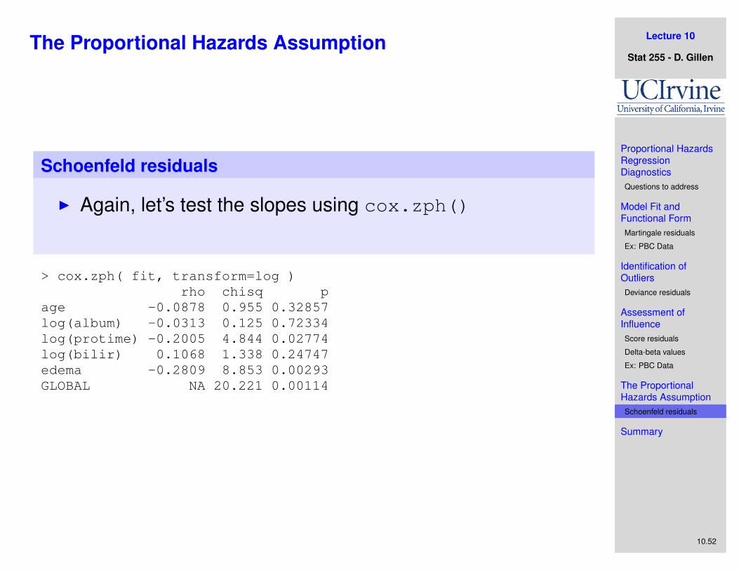
I Again, let’s test the slopes using cox.zph()
> cox.zph( fit, transform=log )rho chisq p
age -0.0878 0.955 0.32857log(album) -0.0313 0.125 0.72334log(protime) -0.2005 4.844 0.02774log(bilir) 0.1068 1.338 0.24747edema -0.2809 8.853 0.00293GLOBAL NA 20.221 0.00114
Lecture 10
Stat 255 - D. Gillen
Proportional HazardsRegressionDiagnosticsQuestions to address
Model Fit andFunctional FormMartingale residuals
Ex: PBC Data
Identification ofOutliersDeviance residuals
Assessment ofInfluenceScore residuals
Delta-beta values
Ex: PBC Data
The ProportionalHazards AssumptionSchoenfeld residuals
Summary
10.53
The Proportional Hazards Assumption
Schoenfeld residuals
I Conclusion: We reject the null hypothesis of proportionalhazards for both log(prothombin)and edema, andconclude that their effect varies as a function of log(time).
I Compare the results for edema with what we found lookingat time-varying covariates!
I Note: We are attempting to disprove the proportionalhazards assumption. Just because we fail to reject the nullhypothesis does not guarantee proportional hazards, ourtest may just be underpowered.

Lecture 10
Stat 255 - D. Gillen
Proportional HazardsRegressionDiagnosticsQuestions to address
Model Fit andFunctional FormMartingale residuals
Ex: PBC Data
Identification ofOutliersDeviance residuals
Assessment ofInfluenceScore residuals
Delta-beta values
Ex: PBC Data
The ProportionalHazards AssumptionSchoenfeld residuals
Summary
10.54
Model Diagnostics: Summary
Summary
I Model:
I Proportional hazards assumption:
I Functional form of covariates (log, square-root, etc.):
Lecture 10
Stat 255 - D. Gillen
Proportional HazardsRegressionDiagnosticsQuestions to address
Model Fit andFunctional FormMartingale residuals
Ex: PBC Data
Identification ofOutliersDeviance residuals
Assessment ofInfluenceScore residuals
Delta-beta values
Ex: PBC Data
The ProportionalHazards AssumptionSchoenfeld residuals
Summary
10.55
Model Diagnostics: Summary
Summary
I Observations:
I Observations not well-described by the model (outliers):
I Observations with undue influence on results:
(here, “results” refers to one β at a time)