Journal of Power and Energy Engineering, 2014, 2, 45-58 Published Online August 2014 in SciRes. http://www.scirp.org/journal/jpee http://dx.doi.org/10.4236/jpee.2014.28005

How to cite this paper: Jin, Z.Q. and Huang, C. (2014) DFIG Voltage Control Based on Dynamically Adjusted Control Gains. Journal of Power and Energy Engineering, 2, 45-58. http://dx.doi.org/10.4236/jpee.2014.28005

DFIG Voltage Control Based on Dynamically Adjusted Control Gains Zhiqiang Jin, Can Huang Department of Electrical Engineering and Computer Science, University of Tennessee, Knoxville, USA Email: zjin@utk.edu, chuang16@utk.edu Received 19 June 2014; revised 20 July 2014; accepted 11 August 2014

Copyright © 2014 by authors and Scientific Research Publishing Inc. This work is licensed under the Creative Commons Attribution International License (CC BY). http://creativecommons.org/licenses/by/4.0/

Abstract The increasing penetration of wind power presents many technical challenges to power system operations. An important challenge is the need of voltage control to maintain the terminal voltage of a wind plant to make it a PV bus like conventional generators with excitation control. In the previous work for controlling wind plant, especially the Doubly Fed Induction Generator (DFIG) system, the proportional-integral (PI) controllers are popularly applied. These approaches usually need to tune the PI controllers to obtain control gains as a tradeoff or compromise among various operating conditions. In this paper, a new voltage control approach based on a different philoso-phy is presented. In the proposed approach, the PI control gains for the DFIG system are dynami-cally adjusted based on the dynamic, continuous sensitivity which essentially indicates the dy-namic relationship between the change of control gains and the desired output voltage. Hence, this control approach does not require any good estimation of fixed control gains because it has the self-learning mechanism via the dynamic sensitivity. This also gives the plug-and-play feature of DFIG controllers to make it promising in utility practices. Simulation results verify that the pro-posed approach performs as expected under various operating conditions.

Keywords Gain Tuning, Dynamically Adjusted Control Gain, Renewable Energy, Voltage Control, Wind Power

1. Introduction The global warming problem has received increasing concerns due to pollutant emission, significant portion of which is produced by the conventional thermal power plant fueled by coal and natural gas. As an important so-lution to reduce the emission from power generation, renewable energy resources are growing fast in many countries. Among all renewables, wind energy is the most outstanding one. In the US, most of the states have Renewable Portfolios Standard, which is an individual state-wide policy aiming at achieving a certain percen-

Z. Q. Jin, C. Huang

46

tage of their power from renewable energy sources by a certain date, typically targets a range from 10% to 20% of total capacity by 2020. However, the increasing penetration of renewable energy sources, in particular, wind energy conversion system (WECS), in the conventional power system has put tremendous challenges to the power system operators and planners [1] [2].

These challenges include the optimal scheduling of wind power from the longer-term viewpoint, as well as the stability and control issues from the shorter-term viewpoint. Here, this paper is aimed to address the chal-lenge of maintaining a stable voltage profile because the voltage and reactive power control is a pressing issue for DFIG integration. Further, since a wind plant, usually modeled as a PV bus like other generator buses, must maintain a given voltage schedule, investigation of voltage regulation from the dynamic study is a realization of a DFIG bus as a PV bus.

A doubly fed induction generator (DFIG) gives better wind energy transfer efficiency as opposed to other wind generators. They can also offer significant enhancement for transmission support regarding voltage control, transient performance, and damping [3]. DFIG employs a series of voltage-source converters consisting of a ro-tor-side converter (RSC) and a grid-side converter (GSC) to feed the wound rotor. This makes it different from the conventional induction generator. DFIG also has an additional advantage of flexible control and stability over other induction generators due to its control capacity of these converters [2]. Modeling of DFIG and related small signal stability analysis can be found in [4]-[7].

The decoupled control of DFIG has been popular in recent research. It has four controllers, named refP ,

srefV , dcrefV and crefQ , which are required to maintain the maximum power tracking, stator terminal voltage, DC voltage level, and GSC reactive power level, respectively. The coordinated tuning of these controllers by tri-al-and-error method can be really difficult [1]. The coordinated tuning using particle swam optimization (PSO) has been proposed in [8] [9]. The decoupled P-Q control method is used in [10] [11]. The auxiliary control loop to improve inter-area oscillation damping is proposed in [12] [13]. Moreover, a power system stabilizer for DFIG- based wind generation using a speed deviation is proposed in [14]. A coordinated tuning of the damping con-troller to enhance the damping of the oscillatory modes using bacteria foraging technique is presented in [1] and [15]. The control on DFIG-based system under unbalanced grid voltage conditions has been proposed in [16]- [18].

Many previous works in gain tuning for DFIG are based on some optimization approaches to reach a tradeoff or compromise such that the wind system can achieve good, but not always the best performance under various operating conditions and avoid worst-case performance under some extreme conditions. Different from these previous approaches for DFIG control, this research work uses a different philosophy to achieve ideal perfor-mance based on dynamic tuning of control gains for a DFIG-based wind system. A similar philosophy has been successfully applied in [19] for the voltage control of three-phase distributed energy resources. Here, the pro-posed dynamic tuning is carried out during the process for stability control, such as regulating output voltage of DFIG. When the system operating condition varies in real time, the proposed approach can autonomously “learn” the voltage response change w.r.t. the control gain change such that it can dynamically change the control gains in real time to achieve the ideal performance. Hence, the desired performance can be maintained with the pro-posed control using dynamic gain tuning. The structure of this paper is as follows. Section 2 presents the mod-eling of wind turbine DFIG systems. Section 3 describes the proposed control strategy. Simulation and results are discussed in Section 4 followed by conclusions and future work in Section 5.

2. Modeling of the Wind-Turbine Doubly-Fed Induction Generator 2.1. Turbine Model The wind turbine doubly fed induction generator (DFIG) system is shown in Figure 1. The wind power captured by the wind turbine is converted into electrical power by the drive train, and then transmitted to the grid by a doubly fed induction generator. The stator side of the DFIG is connected to the grid directly. The rotor side of the DFIG is connected to the grid through a back-to-back converter system. This converter system can be di-vided to two components: rotor side converter ( )rotorC and grid side converter ( )gridC . A capacitor is con-nected between these two converters as the DC voltage source.

The control system generators voltage signals to control the power output, terminal voltage, and DC voltage. There are three control parts: Rotor Side Control, Grid Side Control, and Pitch Angel Control.

Z. Q. Jin, C. Huang

47

DFIG GridDrive Train

L

Control

Vr Vgc

Pitch Angle

(Ps, Qs)

(Pr, Qr) (Pgc, Qgc)

(Tm, Wr) Pm

X(P, V)

RSC GSC

AC/DC/AC Converter System

Figure 1. Wind turbine DFIG system.

2.2. Rotor Side Control System The rotor-side converter is used to control the wind turbine power output and the voltage measured at the grid terminal. The wind power output is controlled to follow a pre-defined curve, see Figure 2. The terminal voltage controller is designed to control the terminal voltage to maintain a constant value such that the terminal of this wind turbine DFIG system can be modeled as a PV bus according to a particular wind speed.

The rotor side control loop is illustrated in Figure 3. For the rotor-side controller the d-axis of the rotating reference frame used for d-q transformation is aligned with the air-gap flux.

As shown in Figure 3(a), the terminal voltage is compared to the reference voltage, then the error will be re-duced to zero by the AC Voltage Regulator, with _refdrI as the output. Next, drI will be compared to _refdrI and the error will be reduced to zero by another PI controller in the Process part, with drV as the output.

As shown in Figure 3(b), lossP , the power losses, is added to the output power. The sum is compared with the reference power. A power regulator is used to reduce the error to zero and output _refqrI . Then, another PI controller is used to reduce the error to zero in the Process part and output drV . These voltage signals will be fed back to the system as voltage control signals.

2.3. Grid Side Control System The grid side control system is illustrated in Figure 4. The gridC converter is used to regulate the voltage of the DC bus capacitor. For the grid-side controller the d-axis of the rotating reference frame used for d-q transforma-tion is aligned with the positive sequence of the grid voltage.

A proportional-integral (PI) controller is used to reduce the error between dcV and _refdcV , and the output is _refdgcI for the current regulator. Here dgcI is the current in phase with grid voltage which controls active pow-

er flow. Then, an inner current regulation loop consisting of a current regulator controls the magnitude and phase angle of the voltage generated by the converter gridC , i.e., gcV . Here, gcV has two parts, qgcV and dgcV , where qgcV depends on the difference between qgcI and the specified reference _refqI , and dgcV depends on the difference between dgcI and _refdgcI which is produced by the DC voltage regulator and. The current regu-lator is assisted by feed forward terms which predict the gridC output voltage.

2.4. Pitch Angle Control System The pitch angle is kept constant at zero degree until the wind speed reaches a specified value (see Figure 2). Then, beyond this value, the pitch angle is proportional to the speed deviation from this specified speed. How-ever, the rotational speed is usually chosen less than the point-D speed because it is of less interest for electro-magnetic transients [20].

3. Proposed Control Strategy When there is a drop of the terminal voltage of the DFIG due to wind speed change or load change, it needs to quickly recover to its scheduled value pre-defined by operators. In the proposed approach, we first define an exponential curve, as illustrated in Figure 5, as the desired response based on the value immediately after the voltage drop as the initial value ( )0V and the final steady-state value ( finalV , usually the desired voltage sche-

dule). The transition from 0V to finalV follows an exponential increase defined with the shape of 1t

e τ−

− , where

Z. Q. Jin, C. Huang

48

τ is a user-defined time constant. In other words, the voltage deviation from finalV is ( ) 0et

tV t V τ−

∆ = ∆ , which is an exponential decay. Hence, as long as we can keep the voltage response following the desired curve as shown in Figure 5, the stability will be maintained without instability or overshoot problems.

Here, a period of 5τ (i.e., 5 times of the time constant) is chosen as the desired response time because the voltage after 5τ is almost the same as finalV ( 5e 0.007 0− = ≈ and ( ) final final5 0.993V t V Vτ= = ≈ ). Hence, if

Figure 2. Wind turbine power characteristics [20].

(a)

(b)

Figure 3. Rotor side control.

Figure 4. Grid side control.

AC Voltage Regulator

+

-

Vref

Idr_ref +

Idr

Process-

VdrV

AC Voltage Regulator

+

-

Vref

Idr_ref +

Idr

Process-

VdrV

Z. Q. Jin, C. Huang

49

Figure 5. Reference voltage curve for the proposed control approach.

the operators prefer the voltage rise time is rt seconds, then the time constant τ is 0.2 rt seconds.

Next, the PI controllers with dynamical adjustment are applied to reduce the error between the actual voltage response and the ideal (desired) response to zero. Initially, very small values of the PI controller gains are ap-plied, which lead to a large error. However, the control gains may be gradually increased to speed up the reduc-tion of the error such that the actual voltage may catch up the desired voltage regulation curve. The increasing pattern may be stopped when the actual voltage curve is aligned with the desired curve. The above process is somewhat similar to accelerate a moving object to catching another moving target at the desired velocity. Once the object reaches the desired velocity, the acceleration may be stopped (to avoid overshoot).

Hence, the above control process differs from conventional PI control and/or gain tuning because of the dy-namic adjustment of the PI control gains during the voltage regulation process, while conventional PI control uses fixed control gains during the process or different control gains under different scenarios. Since the pro-posed control process starts with a small value of control gains, it will not have the overshoot problem at the very beginning. Then, the gains will be gradually increased such that the actual voltage response can “speed up” to eventually catch up the desired response curve.

Next, more technical details are elaborated.

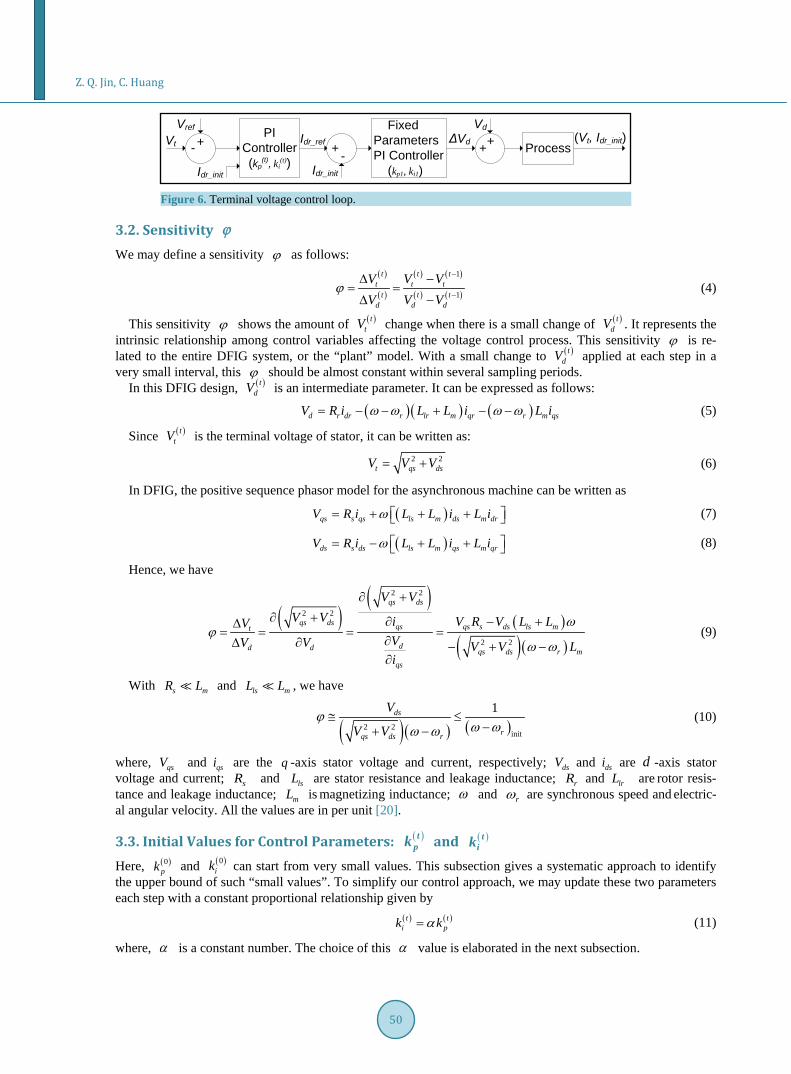
3.1. Voltage Control System Configuration Figure 6 shows the actual control part of the rotor side control. First, the error between the reference voltage and the actual voltage goes into the first PI controller, which has flexible PI control gains (i.e., ( )t

pk and ( )tik ) and

gives updated value of _refdrI . The difference between the _refdrI and _initdrI is the initial value for the second fixed-gain controller. Hence, we can obtain the equation to calculate the output of the first PI controller as fol-lows:

( ) ( ) ( ) ( ) ( )( ) ( ) ( ) ( )( )1

_ref _init ref ref dtt t t t t t t t

dr dr p t i tt

I I k V V k V V τ+

= + − + −∫ (1)

The second fixed-gain (i.e., 1pk and 1ik in Figure 6) PI controller is used to control _initdrI to reach its reference value _refdrI . The equation to calculate the output of the second PI controller is given by:

( ) ( ) ( ) ( )( ) ( ) ( ) ( )( ) ( ) ( ) ( )( ) ( ) ( ) ( )( )1 1 1

1 ref ref 1 ref refd d dt t t

t t t t t t t t t t t t td p p t i t i p t i t

t t t

V k k V V k V V k k V V k V Vτ τ τ+ + +

∆ = − + − + − + −

∫ ∫ ∫ (2)

The sampling frequency is usually very high (at the level of multiple kHz) so dτ is very small. Then, we can linearize the above equation based on the sampling frequency as follows:

( ) ( ) ( )( ) ( ) ( ) ( ) ( )( )ref 1 1 1 1d d d dt t t t t t td t p p i p p i i iV V V k k k k k k k kτ τ τ τ∆ = − + + + (3)

0 0.05 0.1 0.15 0.2 0.25 0.3 0.35 0.4 0.45 0.51

1.002

1.004

1.006

1.008

1.01

1.012

Z. Q. Jin, C. Huang

50

Figure 6. Terminal voltage control loop.

3.2. Sensitivity ϕ We may define a sensitivity ϕ as follows:

( )

( )

( ) ( )

( ) ( )

1

1

t t tt t t

t t td d d

V V VV V V

ϕ−

−

∆ −= =∆ −

(4)

This sensitivity ϕ shows the amount of ( )ttV change when there is a small change of ( )t

dV . It represents the intrinsic relationship among control variables affecting the voltage control process. This sensitivity ϕ is re-lated to the entire DFIG system, or the “plant” model. With a small change to ( )t

dV applied at each step in a very small interval, this ϕ should be almost constant within several sampling periods.

In this DFIG design, ( )tdV is an intermediate parameter. It can be expressed as follows:

( )( ) ( )d r dr r lr m qr r m qsV R i L L i L iω ω ω ω= − − + − − (5)

Since ( )ttV is the terminal voltage of stator, it can be written as:

2 2t qs dsV V V= + (6)

In DFIG, the positive sequence phasor model for the asynchronous machine can be written as

( )qs s qs ls m ds m drV R i L L i L iω = + + + (7)

( )ds s ds ls m qs m qrV R i L L i L iω = − + + (8)

Hence, we have

( )( )

( )

( )( )

2 2

2 2

2 2

qs ds

qs ds qs qs s ds ls mt

dd d qs ds r mqs

V VV V i V R V L LV

VV V V V Li

ωϕ

ω ω

∂ +

∂ + ∂ − +∆= = = =

∂∆ ∂ − + −∂

(9)

With s mR L and ls mL L , we have

( )( ) ( )2 2init

1ds

rqs ds r

V

V Vϕ

ω ωω ω≅ ≤

−+ − (10)

where, qsV and qsi are the q -axis stator voltage and current, respectively; dsV and dsi are d -axis stator voltage and current; sR and lsL are stator resistance and leakage inductance; rR and lrL are rotor resis-tance and leakage inductance; mL is magnetizing inductance; ω and rω are synchronous speed and electric-al angular velocity. All the values are in per unit [20].

3.3. Initial Values for Control Parameters: ( )tpk and ( )t

ik Here, ( )0

pk and ( )0ik can start from very small values. This subsection gives a systematic approach to identify

the upper bound of such “small values”. To simplify our control approach, we may update these two parameters each step with a constant proportional relationship given by

( ) ( )t ti pk kα= (11)

where, α is a constant number. The choice of this α value is elaborated in the next subsection.

Fixed Parameters PI Controller

(kp1, ki1)

PI Controller(kp

(t), ki(t))

+- + - + + Process

Vref

Vt Idr_ref

Idr_init

Vd(Vt, Idr_init)ΔVd

Idr_init

Z. Q. Jin, C. Huang

51

Then, we have ( ) ( ) ( )( ) ( ) ( ) ( ) ( )( )

( ) ( )( ) ( ) ( )ref 1 1 1 1

ref 1 1 1 1

d d d d

d d d d .

t t t t t t td t p p p p p i p i

t t tt p p p i i

V V V k k k k k k k k

V V k k k k k

α τ τ α τ τ

α τ τ α τ τ

∆ = − + + +

= − + + + (12)

Since tV is less than refV , we have ( ) ( )( )

( )

( ) ( )( )( ) ( ) ( )

1 0 0 0

0 0 01 1 1 1

1d d d d

t t ref t

d d p p p i i

V V V V

V V k k k k kϕ

α τ τ α τ τ

− −= ≤ =

∆ ∆ + + + (13)

Therefore, we have

( )

( )0

1 1 1 1

1d d d dp

p p i i

kk k k kα τ τ α τ τ ϕ

≤+ + +

(14)

To ensure ( )0pk is less than the right-hand side (RHS) of (14), we may set ( )0

pk less than the minimum value of the RHS of (14). Hence, as long as we have (15), Equation (14) will be always satisfied.

( ) ( )( )

0 init

1 1 1 1d d d dr

pp p i i

kk k k k

ω ω

α τ τ α τ τ

−≤

+ + + (15)

Equation (15) gives the upper bound of the initial value of the control gains. It can guarantee that ( )0pk and

( )0ik are small enough such that overshoot does not occur from the beginning. Since the above derivation al-

ways takes the conservative side, this should give relatively slow start w.r.t. the desired response curve. This is preferred because it is always desired to start with conservative values, and the initially slow response can be accelerated at a later time while aggressive initial values may immediately lead to undesired overshoot.

3.4. Dynamic Update of ( )tpk and ( )t

ik The key of the proposed control is to dynamically adjust the control gains, pk and ik . Here as previously mentioned in (11) in Section 3.3, ik and pk are assumed to keep a constant ratio given by, i.e., ( ) ( )t t

i pk kα= . The value of α represents the ratio of the effect caused by the proportional part and the integral part of the

PI controller. Essentially, the result is expected to be like the curve in Figure 7. The effect of the integral part is set roughly equal to the effect of the proportional part when the difference

between the reference and the terminal voltage reaches the maximum. If the time needed for the process is t∗ , it is assumed that the time needed for the difference to reach the maximum at 0.5 t∗× . So α can be roughly calculated as follows:

( )

( )( )

( )

( )( )

ref refmax max

ref maxref

20.5d

tt ti

t t ttp tt

V V V VkV V t tk V V t

α ∗ ∗ ∗+

− −= = ≅ =

−−∫ (16)

Figure 7. Expected result case.

Z. Q. Jin, C. Huang

52

Also, we consider the control gains are changed by a co-efficient β from the time t to time 1t + . This is given by

( ) ( )1t tp pk kβ+ = (17)

Assuming the “catching-up” process ends after t∗ , then we have: 0 maxst fp pk kβ

∗≤ (18)

where sf is the sampling frequency and st f∗ × is the number of updates for pk . The limit of pk , or maxpk ,

is given by (19), which is elaborated in detail in the next subsection.

( )max

max1 1 1 1

1d d d dp

p p i i

kk k k kϕ α τ τ α τ τ

≤+ + +

(19)

where maxϕ is the largest value of ϕ which is dynamically updated during the control process. Then, we have

( )0 max

max1 1 1 1

1d d d d

st fp p

p p i i

k kk k k k

βϕ α τ τ α τ τ

∗≤ ≤

+ + + (20)

Hence, the value of β can be chosen as:

( )1

0 max1 1 1 1d d d d st f

p p p i ik k k k kβ ϕ α τ τ α τ τ ∗−

= + + + (21)

3.5. Limit for ( )tpk

The goal of the proposed method is to control the terminal voltage such that it can reach the final value smoothly following the ideal response curve as much as possible. At the beginning of this voltage control process, the er-ror between the reference and the voltage increases and essentially reaches the peak value. Then, it starts to de-crease. As previously described, here the dynamically adjusted control gains play as the “acceleration factor” or “de-acceleration factor” during this control process. By doing so, the voltage error may go to zero without going to negative (i.e., overshoot). Thus, there should be a maximal value of ( )t

pk . From (4), we know ( ) ( )( ) ( )1t t t

t t dV V V ϕ+ − = ∆ (22)

With (12), we can obtain ( ) ( )( ) ( ) ( )( ) ( ) ( )1

ref 1 1 1 1d d d dt t t t tt t t p p p i iV V V V k k k k kα τ τ α τ τ ϕ+ − = − + + + (23)

It is necessary to ensure the following equation such that there will not be any overshoot ( ) ( )( ) ( ) ( )( )1

reft t t t

t t tV V V V+ − < − (24)

Hence, we have ( ) ( )( ) ( ) ( ) ( ) ( )( )ref 1 1 1 1 refd d d dt t t t t

t p p p i i tV V k k k k k V Vα τ τ α τ τ ϕ− + + + < − (25)

Therefore, we have ( ) ( )1 1 1 1d d d d 1tp p p i ik k k k kα τ τ α τ τ ϕ+ + + < (26)

( )

( )1 1 1 1

1d d d d

tp

p p i i

kk k k kα τ τ α τ τ ϕ

<+ + +

(27)

To ensure that ( )tpk is less than the right-hand side (RHS) of (27), we may set ( )t

pk less than the minimum val-ue of the RHS of (27), which occurs at maxϕ ϕ= . Hence, as long as we have (28), Equation (27) is always ensured.

( )max

max1 1 1 1

1d d d dp

p p i i

kk k k kϕ α τ τ α τ τ

<+ + +

(28)

Z. Q. Jin, C. Huang

53

3.6. Flow Chart The whole control process is briefly presented in the flowchart shown in Figure 8.

4. Simulation and Results The power system under study is as shown in Figure 9. The wind farm, which consists of six 1.5 MW wind tur-bines, is connected to a 25 kV distribution system. This farm exports power to a 120 kV grid through a 30 km 25 kV feeder. A 2 MVA plant consisting of a motor load and of a 200 kW resistive load is connected on the same feeder at bus B25. A 500 kW load is connected to the DFIG system [20].

In this section, first, a demonstration of inappropriate fixed PI gains is shown to verify the importance of PI gains. Then, several case studies are carried out to illustrate that the proposed approach of dynamically adjusted PI gains can achieve desired performance under various operating conditions.

4.1. Demonstration of Instability with Inappropriate PI Gains As previously mentioned in Sections 1 and 2, the motivation of this paper is to present an approach to avoid the potential instability raised by fixed control gains. With inappropriate pk and ik values, different responses like unstable response, stable but oscillating response, or sluggish response may happen. The results from an example are shown in Figure 10 for the case that the reference voltage changes from a stable state value 1.0 p.u.

Figure 8. Flow chart showing the control process.

Figure 9. Sample power system with DFIG for simulation study.

Start

Monitoring voltage

VoltageLoss ?

Initialize

kp and ki

Yes

No

Yes

No

No

Yes

Voltage Recover ?

kp >= Limit

Update kp and ki

Set kp and ki to limit values

Terminate

ACGridDFIG

Load500kW

Plant2 MVA

B575(575V)

B25(25kV)

B120(120kV)

9 MW Wind Farm(6*1.5MW)

575V/25kV6*2MVA 10 km

line20 km

line

GroundTransformer

25kV/120kV47 MVA

Z. Q. Jin, C. Huang

54

(a) (b)

(c) (d)

Figure 10. Results demonstration in stability when inappropriate fixed control gains are chose as 4.5pk = and

1080ik = . (a) Real power output; (b) Reactive power output; (c) Terminal voltage; (d) DC voltage.

to 1.01 p.u. to mimic a small disturbance. Control gains of 4.5pk = and 1080ik = are chosen. The results in-clude active power, reactive power, terminal voltage, and DC voltage.

4.2. Case One: Set Final Voltage to 1.01 p.u. As mentioned in the opening part in Section 3, users may define the desired time to regulate the terminal voltage from the time of disturbance to the final steady-state value. Here the transient time for voltage is set to 0.5 seconds since this is fast enough before other conventional (usually much slower) voltage controls take effect or are activated. Since an exponential decay of the voltage difference, i.e., ( ) ( )final 0 – e t

tV t V V τ−∆ = , is preferred with 5τ as the desired transition time, τ is 0.1 sec in this and the next a few studies.

In this case study, a step change of voltage reference is made from 1.0 to 1.01 per unit. The dynamically ad-justed control gains are employed. As shown in Figure 11, a smooth transition can be achieved. Note that the control gains such as pk change dynamically. As shown in Figure 11(b), initially, the terminal voltage lags the desired voltage. Then, it gradually catches up the desired voltage growth curve. Once it reaches the desired curve, the control gain pk stops increasing and the actual curve matches the desired curve very well. Figure 11(c) shows the dynamic values of pk . The above process is similar to accelerate a moving object to reach the desired velocity. Once the desired velocity is reached, the accelerating factor (i.e., pk ) may stop increasing and remain the value at that point.

Figure 11(d) shows the value of ϕ and Figure 11(e) shows the value of dcV , which is maintained at 1200 V as expected.

4.3. Case Two: Set Final Voltage to 1.04 p.u. Figure 12 shows the results of Case Two, in which the voltage reference is changed from 1.0 to 1.04 p.u. to mimic a larger disturbance. The results are very similar to the previous case study, and similar observations can be made.

4.4. Case Three, Four, and Five: Load = 200, 800, and 1100 kW, Respectively Different loads may have different effects on the terminals voltage of the wind turbine DFIG system. Hence, three additional case studies are performed. These cases are similar to Case One, but differ in the amount of load. Considering the load in Case One is 500 kW, the load levels in Cases Three, Four, and Five are changed to 200 kW, 800 kW, and 1100 kW, respectively. The results of the three most important variables, voltage error in p.u., voltage in p.u., and dcV in volts are shown in Figures 13-15, respectively. Other variables are not shown due to space limit.

0 0.2 0.4 0.6 0.8 11

1.5

2

2.5

Time ( s )

P (

MW

)

P

0 0.2 0.4 0.6 0.8 1-1

0

1

2

Time ( s )

Q (

MV

AR

)

Q

Z. Q. Jin, C. Huang

55

As observed in these figures, the proposed control approach gives dynamically adjusted control gain pk to catch up and then follow the desired performance very well.

Figure 11. Results as new final voltage set as 1.01 p.u. to mimic a small disturbance. (a) Voltage error (difference); (b) Actual & ideal voltage curve; (c) Control gain kp; (d) Sensitivity φ (φmax = 0.02); (e) DC voltage.

Figure 12. Results as new final voltage set as 1.04 p.u. to mimic a small disturbance.

Z. Q. Jin, C. Huang

56

Figure 13. Results for case three (load = 200 kW).

Figure 14. Results for case four (load = 800 kW).

Figure 15. Results for case five (load = 1100 kW).

5. Conclusions and Future Work In this paper, a new DFIG voltage control approach based on a philosophy different from the previous works is presented. In the proposed approach, the PI control gains for the DFIG system are dynamically adjusted based on the dynamic, continuous sensitivity which essentially indicates the dynamic relationship between the change

Z. Q. Jin, C. Huang

57

of control gains and the desired output voltage. Hence, this control approach does not require any good estima-tion of fixed control gains because it has the self-learning mechanism via the dynamic sensitivity. This also gives the plug-and-play feature of the proposed DFIG controller to make it promising in utility practices. Simu-lation results verify that the proposed approach performs as expected under various operating conditions.

Future works may include the study of multiple wind plants in a system as well as the control of real power especially when an energy storage system is connected to the wind plant.

Acknowledgements This work made use of engineering research center shared facilities supported by the engineering research center program of the national science foundation and the department of energy under NSF award Number EEC- 1041877 and the CURENT industry partnership program. Thanks so much to my supervisor, Dr. Fangxing “Fran” Li’s great help and guidance.

References [1] Manjure, D.P., Mishra, Y., Brahma, S. and Osborn, D. (2012) Impact of Wind Power Development on Transmission

Planning at Midwest ISO. IEEE Transactions on Sustainable Energy, 3, 845-852. http://dx.doi.org/10.1109/TSTE.2012.2205024

[2] Mishra, Y., Mishra, S., Li, F. and Dong, Z.Y. (2009) Small-Signal Stability Analysis of a DFIG-Based Wind Power System under Different Modes of Operation. IEEE Transactions on Energy Conversion, 24, 972-982. http://dx.doi.org/10.1109/TEC.2009.2031498

[3] Holdsworth, L, Wu, X.G., Ekanayake, J.B. and Jenkins, N. (2003) Comparison of Fixed Speed and Doubly-Fed Induc-tion Wind Turbines during Power System Disturbances. IEE Proceedings—Generation, Transmission and Distribution, 150, 343-352. http://dx.doi.org/10.1049/ip-gtd:20030251

[4] Mei, F. and Pal, B.C. (2007) Modal Analysis of Grid Connected Doubly Fed Induction Generator. IEEE Transactions on Energy Conversion, 22, 728-736. http://dx.doi.org/10.1109/TEC.2006.881080

[5] Lei, Y., Mullane, A., Lightbody, G. and Yacamini, Y. (2006) Modeling of the Wind Turbine with a Doubly Fed Induc-tion Generator for Grid Integration Studies. IEEE Transactions on Energy Conversion, 21, 257-264. http://dx.doi.org/10.1109/TEC.2005.847958

[6] Wu, F., Zhang, X.P., Godfrey, K. and Ju, P. (2007) Small Signal Stability Analysis and Optimal Control of a Wind Turbine with Doubly Fed Induction Generator. IET Generation, Transmission, Distribution, 1, 751-769.

[7] Cardenas, R., Pena, R., Tobar, G., Wheeler, P. and Asher, G. (2009) Stability Analysis of a Wind Energy Conversion System Based on a Doubly Fed Induction Generator Fed by a Matrix Converter. IEEE Transactions on Industrial Electronics, 56, 4194-4206. http://dx.doi.org/10.1109/TIE.2009.2027923

[8] Qiao, W., Venayagamoorthy, G.K. and Harley, R.G. (2009) Design of Optimal PI Controllers for Doubly Fed Induc-tion Generators Driven by Wind Turbines Using Particle Swarm Optimization. International Joint Conference on Neural Networks, Vancouver, 16-21 July 2009, 1982-1987.

[9] Wu, F., Zhang, X.P., Godfrey, K. and Ju, P. (2007) Small Signal Stability Analysis and Optimal Control of a Wind Turbine with Doubly Fed Induction Generator. IET Generation, Transmission, Distribution, 1, 751-760.

[10] Banakar, H., Luo, C. and Ooi, B.T. (2006) Steady-State Stability Analysis of Doubly-Fed Induction Generators under Decoupled P-Q Control. IEE Proceedings on Electric Power Applications, 153, 300-306. http://dx.doi.org/10.1049/ip-epa:20050388

[11] Mwinyiwiwa, B., Zhang, Y.Z., Shen, B. and Ooi. B.T. (2009) Rotor Position Phase-Locked Loop for Decoupled P-Q Control of DFIG for Wind Power Generation. IEEE Transactions on Energy Conversion, 24, 758-765. http://dx.doi.org/10.1109/TEC.2009.2025328

[12] Miao, Z., Fan, L., Osborn, D. and Yuvarajan, S. (2008) Control of DFIG Based Wind Generation to Improve Inter- Area Oscillation Damping. IEEE PES General Meeting, Pittsburgh, 20-24 July 2008, 1-7.

[13] Fan, L., Miao, Z. and Osborn, D. (2008) Impact of Doubly Fed Wind Turbine Generation on Inter-Area Oscillation Damping. IEEE PES General Meeting, Pittsburgh, 20-24 July 2008, 1-8.

[14] Hughes, F.M., Lara, O.A., Jenkins, N. and Ancell, G. (2006) A Power System Stabilizer for DFIG-Based Wind Gener-ation. IEEE Transactions on Power Systems, 21, 763-772. http://dx.doi.org/10.1109/TPWRS.2006.873037

[15] Mishra, S. (2005) A Hybrid Least Square-fuzzy Bacteria Foraging Strategy for Harmonic Estimation. IEEE Transac-tions on Evolutionary Computation, 9, 61-73. http://dx.doi.org/10.1109/TEVC.2004.840144

[16] Brekken, T.K.A. and Mohan, N. (2007) Control of a Doubly Fed Induction Wind Generator under Unbalanced Grid

Z. Q. Jin, C. Huang

58

Voltage Conditions. IEEE Transactions on Energy Conversion, 22, 129-135. http://dx.doi.org/10.1109/TEC.2006.889550

[17] Santos-Martin, D., Rodriguez-Amenedo, J.L. and Arnalte, S. (2008) Direct Power Control Applied to Doubly Fed In-duction Generator under Unbalanced Grid Voltage Conditions. IEEE Transactions on Power Electronics, 23, 2328- 2336. http://dx.doi.org/10.1109/TPEL.2008.2001907

[18] Hu, J. and He, Y. (2009) Reinforced Control and Operation of DFIG-Based Wind Power Generation System under Unbalanced Grid Voltage Conditions. IEEE Transactions on Energy Conversion, 24, 905-915. http://dx.doi.org/10.1109/TEC.2008.2001434

[19] Li, H.J., Li, F.X., Xu, Y., Rizy, D.T. and Kueck, J.D. (2010) Adaptive Voltage Control with Distributed Energy Re-sources: Algorithm, Theoretical Analysis, Simulation, and Field Test Verification. IEEE Transactions on Power Sys-tems, 25, 1638-1647. http://dx.doi.org/10.1109/TPWRS.2010.2041015

[20] The Math Works (2012) SimPowerSystems for Use with Simulink, User’s Guide Version 4.