VOT 71565

DEVELOPMENT OF SYMBOLIC ALGORITHMS FOR CERTAIN

ALGEBRAIC PROCESSES

(PEMBINAAN ALGORITMA SIMBOLIK UNTUK BEBERAPA

PROSES ALGEBRA)

ALI BIN ABD RAHMAN

NOR’AINI BINTI ARIS

RESEARCH VOTE NO:

71565

Jabatan Matematik

Fakulti Sains

Universiti Teknologi Malaysia

2007

i

ACKNOWLEDGEMENTS

In The Name Of ALLAH, The Most Beneficent, The Most Merciful

All praise is due only to ALLAH, the Lord of the Worlds. Ultimately, onlyAllah has given us the strength and courage to proceed with our entire life. His worksare truly splendid and wholesome and His knowledge is truly complete with dueperfection.

The financial support from UTM, particularly, from the Research ManagementCenter, for its research grant is greatly appreciated. An acknowledgement is also dueto the Research Institute for Symbolic Computation (RISC), Johannes KeplerUniversity, Linz, Austria for granting the permission to a copy of SACLIB. A specialgratitude to Professor George Collins who initiated the C-based, open source codesoftware and who has always been responsive to questions regarding theimplementation of its programs. A lot of professor Collin’s work, in particular, hisdeterministic approach on the theoretical computing time analysis of algorithms hasbeen referred to in this research work.

ii

ABSTRACT

This study investigates the problem of computing the exact greatest commondivisor of two polynomials relative to an orthogonal basis, defined over the rationalnumber field. The main objective of the study is to design and implement an effectiveand efficient symbolic algorithm for the general class of dense polynomials, given therational number defining terms of their basis. From a general algorithm using thecomrade matrix approach, the nonmodular and modular techniques are prescribed.

If the coefficients of the generalized polynomials are multiprecision integers,multiprecision arithmetic will be required in the construction of the comrade matrixand the corresponding systems coefficient matrix. In addition, the application of thenonmodular elimination technique on this coefficient matrix extensively appliesmultiprecision rational number operations. The modular technique is employed tominimize the complexity involved in such computations. A divisor test algorithm thatenables the detection of an unlucky reduction is a crucial device for an effectiveimplementation of the modular technique. With the bound of the true solution notknown a priori, the test is devised and carefully incorporated into the modularalgorithm.

The results illustrate that the modular algorithm illustrate its bestperformance for the class of relatively prime polynomials. The empirical computingtime results show that the modular algorithm is markedly superior to the nonmodularalgorithms in the case of sufficiently dense Legendre basis polynomials with a smallGCD solution. In the case of dense Legendre basis polynomials with a big GCDsolution, the modular algorithm is significantly superior to the nonmodular algorithmsin higher degree polynomials. For more definitive conclusions, the computing timefunctions of the algorithms that are presented in this report have been worked out.Further investigations have also been suggested.

Key Researches:Assoc. Prof. Dr. Ali Abd Rahman

Nor’aini Aris

iii

ABSTRAK

Kajian ini mengkaji masalah pengiraan tepat pembahagi sepunya terbesar duapolinomial relatif terhadap suatu asas ortogon yang tertakrif ke atas medan nombornisbah. Objektif utama kajian ialah untuk membangunkan dan melaksanakan suatualkhwarizmi simbolik untuk kelas umum polinomial tumpat, diketahui sebutanpentakrif bagi asasnya. Kaedah penyelesaian modulo dan tak modulo diasaskankepada suatu alkhwarizmi am. Jika pekali bagi polinomial dalam perwakilan teritlakmerangkumi integer kepersisan berganda, aritmetik kepersisan berganda diperlukandalam pembinaan matriks komrad dan matriks pekali sistem berpadanan. Penggunaanteknik penurunan tak modulo terhadap matriks pekali tersebut banyak melibatkanaritmetik nombor nisbah dan operasi integer kepersisan berganda.

Teknik modulo di selidiki bagi mengurangkan kerumitan penggunaan operasitersebut. Keberkesanan pendekatan modulo bergantung kepada kejayaan mewujudkansuatu teknik yang dapat menyemak kebenaran penyelesaian pada peringkat-peringkatpenyelesaian secara berpatutan. Dalam keadaan di mana batas jawapan sebenar tidakdapat ditentukan, suatu pendekatan modulo telah dihasilkan.

Teknik tersebut mempamerkan pencapaian terbaik dalam perlaksanaannyaterhadap kelas polinomial yang perdana relatif. Keputusan ujikaji masa pengiraanmenunjukkan kecekapan alkhwarizmi modulo jauh mengatasi alkhwarizmi tak modulodalam kelas polinomial tumpat terhadap asas Legendre yang mempunyai satupolinomial pembahagi sepunya terbesar bersaiz kecil. Bagi kelas polinomial yang samatetapi mempunyai satu penyelesaian bersaiz besar, alkhwarizmi modulo adalah jauhlebih cekap untuk polinomial berdarjah besar. Keputusan masa pengiraan untukpolinomial nombor nisbah yang diwakili oleh polinomial terhadap asas Legendremempamerkan kecekapan alkhwarizmi yang menggabungkan pendekatan modulo dantak modulo pada beberapa bahagian tertentu daripada keseluruhan kaedahpenyelesaian. Untuk keputusan secara teori dan berpenentuan, fungsi masa pengiraanbagi alkhwarizmi yang dibina telah diusahakan. Penyelidikan lanjut juga dicadangkan.

iv

Contents

1 INTRODUCTION 1

1.1 Preface . . . . . . . . . . . . . . . . . . . . . . . . . . . . . . . . . . . . 1

1.2 Motivation . . . . . . . . . . . . . . . . . . . . . . . . . . . . . . . . . . 2

1.3 Preliminary Definitions and Concepts . . . . . . . . . . . . . . . . . . . 6

1.4 Problem Statement . . . . . . . . . . . . . . . . . . . . . . . . . . . . . . 8

1.5 Research Objectives . . . . . . . . . . . . . . . . . . . . . . . . . . . . . 8

1.6 Scope of Work . . . . . . . . . . . . . . . . . . . . . . . . . . . . . . . . 9

2 LITERATURE REVIEW 10

2.1 Introduction . . . . . . . . . . . . . . . . . . . . . . . . . . . . . . . . . . 10

2.2 Polynomial GCDs over Z . . . . . . . . . . . . . . . . . . . . . . . . . . 11

2.3 Generalized Polynomial GCDs . . . . . . . . . . . . . . . . . . . . . . . 12

2.4 The Exact Elimination Methods . . . . . . . . . . . . . . . . . . . . . . 13

v

2.5 Concluding Remarks . . . . . . . . . . . . . . . . . . . . . . . . . . . . . 14

3 THE COMRADE MATRIX AND POLYNOMIAL GCD COMPUTA-TIONS 15

3.1 Introduction . . . . . . . . . . . . . . . . . . . . . . . . . . . . . . . . . . 15

3.2 Orthogonal Basis and Congenial Matrices . . . . . . . . . . . . . . . . . 15

3.3 GCD of Polynomials Relative to an Orthogonal Basis . . . . . . . . . . 17

3.3.1 On The Construction of Systems of Equations . . . . . . . . . . 18

3.4 A General Algorithm . . . . . . . . . . . . . . . . . . . . . . . . . . . . 18

3.4.1 On the Construction of the Comrade Matrix . . . . . . . . . . . 19

3.4.2 The Coefficient Matrix for a System of Equations . . . . . . . . . 22

3.5 Concluding Remark . . . . . . . . . . . . . . . . . . . . . . . . . . . . . 28

4 THE NONMODULAR GENERALIZED POLYNOMIAL GCD COM-PUTATIONS 29

4.1 Introduction . . . . . . . . . . . . . . . . . . . . . . . . . . . . . . . . . . 29

4.2 The Computation of Row Echelon Form of a Matrix . . . . . . . . . . . 29

4.2.1 Single Step Gauss Elimination . . . . . . . . . . . . . . . . . . . 30

4.2.2 Double Step Gauss Elimination . . . . . . . . . . . . . . . . . . . 31

4.2.3 The Rational Number Gauss Elimination . . . . . . . . . . . . . 33

4.3 On the Nonmodular OPBGCD Algorithms . . . . . . . . . . . . . . . . 34

vi

4.4 Empirical Computing Time Analysis . . . . . . . . . . . . . . . . . . . . 36

4.4.1 Computing Time for OPBGCD-SSGSE and OPBGCD-DSGSE . 37

4.5 Discussions . . . . . . . . . . . . . . . . . . . . . . . . . . . . . . . . . . 38

5 A MODULAR GENERALIZED POLYNOMIAL GCD COMPUTA-TION 39

5.1 An Introduction to the Modular Approach . . . . . . . . . . . . . . . . . 39

5.2 Algorithm MOPBGCD . . . . . . . . . . . . . . . . . . . . . . . . . . . . 41

5.2.1 The Selection of Primes . . . . . . . . . . . . . . . . . . . . . . . 42

5.2.2 Finding the Row Echelon Form and Solution in GF(p) . . . . . . 43

5.2.3 The Application of CRA to MOPBGCD Algorithm . . . . . . . 44

5.2.4 The Rational Number Reconstruction Algorithm . . . . . . . . . 45

5.2.5 The Termination Criterion . . . . . . . . . . . . . . . . . . . . . 46

5.3 Computing Time Results for Algorithm MOPBGCD . . . . . . . . . . . 47

5.3.1 Theoretical Computing Time Analysis . . . . . . . . . . . . . . . 47

5.3.2 Empirical Computing Time Analysis . . . . . . . . . . . . . . . . 47

5.4 Discussions . . . . . . . . . . . . . . . . . . . . . . . . . . . . . . . . . . 49

6 SUMMARY, CONCLUSIONS AND FURTHER RESEARCH 51

6.1 Introduction . . . . . . . . . . . . . . . . . . . . . . . . . . . . . . . . . . 51

6.2 Significant Findings and Conclusions . . . . . . . . . . . . . . . . . . . . 51

vii

6.3 Future Research . . . . . . . . . . . . . . . . . . . . . . . . . . . . . . . 53

7 PAPERS PUBLISHED 59

1

CHAPTER I

INTRODUCTION

1.1 Preface

Fundamental problems in computational algebra that require symboliccomputations or manipulations are the computation of greatest common divisors(GCDs) of integers or polynomials, polynomial factorization and finding the exactsolutions of systems of algebraic equations. Other problems include symbolicdifferentiation and integration, determination of solutions of differential equations andthe manipulation of polynomials and rational functions within its broad spectrum ofapplications. In the last decade, tremendous success has been achieved in this area. Atthe same time, the invention of powerful SAC systems has been motivated to assistingthe scientific community in doing algebraic manipulation as well as providing means ofdesigning and implementing new algorithms. Useful as research tools in manyscientific areas, notable symbolic and algebraic computation (SAC) systems presentlyused worldwide include REDUCE, MACSYMA, MAPLE, MATHEMATICA, SACLIBand most recently MUPAD. Among these systems, SACLIB and MUPAD are opensource LINUX or UNIX systems which are meant for academic purposes thatcontribute to further research in the symbolic algorithms and systems development.

The problem of finding the greatest common divisor (GCD) of the integers isone of the most ancient problems in the history of mathematics [37]. As early as 300B.C., Euclid discovered an algorithm that still bears his name to solve this problem.Today, the concept of divisibility plays a central role in symbolic computations. In thismode, the computation of GCD is not only applied to reducing rational numbers(quotient of integers) to its lowest terms but also to reducing quotients of elementsfrom any integral domain to its simplest form. For example, the computation of GCDof two polynomials reduces a rational function (quotients of polynomials) to its lowestterm. In finding the roots of a polynomial with repeated factors, it is often desirable

2

to divide the polynomial with the GCD of itself and its derivative to obtain theproduct of only linear factors.

An application in the integration of algebraic functions reported that 95% ofthe total time was being spent in GCD computation [42]. As such, GCD operationsbecome the bottleneck of many basic applications of exact computations. In addition,problems involving polynomials, such as polynomial GCD computation andpolynomial factorization, play an important role in many areas of contemporaryapplied mathematics, including linear control systems, electrical networks, signalprocessing and coding theory. In the theory of linear multivariable control systems,GCD determination arises in the computation of the Smith form of a polynomialmatrix, and associated problems, such as minimal realization of a transfer functionmatrix. There are also applications in network theory and in finding solution ofsystems of linear diophantine equations and integer linear programming.

1.2 Motivation

The theory on polynomials in forms other than the power form has been theresults of several works of Barnett and Maroulas, such as in [7], [8], [9] and [10]. Theapplication of polynomials in the generalized form arises in the computation of theSmith form of a polynomial matrix and problems associated with the minimalrealization of a transfer function matrix. The zeros and extrema of the Chebyshevpolynomials play an important role in the theory of polynomial interpolation [54].Barnett [11], describes the theory and applications of such polynomials in linearcontrol systems.

Let a(x) = a0 + a1x + a2x2 + ... + anxn be a polynomial in a variable x over

the field F . If an 6= 0 then degree of a(x) is denoted deg(a). The zero polynomial hasai = 0 for all i and when an = 1, a(x) is termed monic. In this form, a(x) is univariatein the standard form or power series form; that is, a polynomial expressed as a linearcombination of the monomial basis {1, x, , x2, ..., xn−1, xn}.

Let a(x) be monic and F be the field of real numbers R. A companion matrix

3

associated with a(x) is the n× n matrix(

0 In−1

−a0 −a1 . . . −an−1

),

where In denotes the n× n unit or identity matrix. Given a set of orthogonalpolynomials {pi(x)}, Barnett [6] shows that associated with a polynomiala(x) =

∑aipi(x), where ai ∈ R, there exists a matrix A which possesses several of the

properties of the companion matrix. The term comrade matrix is an analogue of thecompanion matrix. The companion matrix is associated with a polynomial expressedin the standard or power series form. The comrade matrix is a generalization of thecompanion matrix and is associated with a polynomial expressed as a linearcombination of an arbitrary orthogonal basis. The term colleague matrix is associatedwith a polynomial expressed as a linear combination of the Chebyshev polynomials, aspecial subclass of the orthogonal basis. Further generalization of the companionmatrix corresponds to the confederate matrix. In the latter, a polynomial a(x) isexpressed in its so called generalized form, such that a(x) =

∑ni=0 aipi(x), in which

case, {pi(x)}ni=0 corresponds to a general basis. In [11], the term congenial matrices

which include the colleagues, comrades and confederate matrices is mentioned.However useful these matrices are, Barnett [6] and [7] does not get around toconverting the theories and analytical results that have been discovered into itspractical use. The theories and analytical results of [6] and [7] have to be convertedinto a procedure so that the routines that extend their applications can beimplemented effectively and efficiently using the computer.

Apart from that, it is natural to speculate whether theorems for polynomials inthe standard form carry over to polynomials in the generalized form. Grant andRahman [29] consider ways in which an algorithm for finding the zeroes of standardform polynomials can be modified to find the zeroes of polynomials in other basis.According to Barnett [11], few results have been reported in this area. For example,the Routh Tabular Scheme (RTS) [7] can be applied to the problem of locating theroots of generalized polynomial in the left and right halves of the complex plane. Aresult that requires determination of odd and even parts of the polynomial is obtained.Similar attempts to generalize the theorems of Hurwitz, Hermite and Schur-Cohn(section 3.2 of [11]) have also proved unsuccessful in obtaining a criterion which can beapplied directly to the coefficients of the generalized form. This means that the

4

polynomials have to be converted to the standard form for the calculations to becarried out and the solutions in the standard form have to be converted back to theoriginal generalized form. This extra work can be avoided by extending or utilizing theproperties of the polynomials given in their respective generalized form.

The RTS calculates the rows of the upper triangular form of the Sylvester’smatrix. The last nonzero row of the upper triangular form of the Sylvester’s matrixgives the coefficients of the GCD of the associated polynomials. Alternate rowsobtained from the RTS give a polynomial remainder sequence. In [7], the relationbetween the polynomial remainder sequence obtained from the rows of the Sylvester’smatrix and the Euclidean polynomial remainder sequence is given. The extension ofthe RTS to the generalized polynomials, examining its application in the computationof the GCD when the degrees of the polynomials are equal is discussed. In a way, themethod shows that the division of polynomials in the generalized form cannot becarried out directly unless the degrees of the polynomials are equal. Analytically, theRouth Tabular Scheme has only been applied for computing the GCD of thepolynomials in the orthogonal basis when the degrees of the input polynomials areequal.

These observations lead us to further investigate polynomials in thegeneralized form. Rather then converting the polynomials to power series form, weaim at obtaining some criteria so that the coefficients of the generalized polynomialscan be applied directly when performing certain operations such as multiplication,division and computing the GCD. Adhering to the given form of polynomials canavoid unnecessary work of basis transformation. Furthermore the properties ofpolynomials in its original form can be fully utilized and further investigated.

A.A. Rahman [1] presents an investigation into GCD algorithms in a floatingpoint environment and uses the results in numerical experiments to solve polynomialexhibiting repeated roots. Although the method developed shows potential, asexpected, the build up of round off errors is so enormous as to render the results forhigh degree polynomials questionable.

In order to compute the GCD of generalized polynomials, the comrade matrixanalogue of the companion matrix requires multiplication and division of the defining

5

terms of the corresponding basis. The entries of the last row of the comrade matrixinvolve the operations of the basis defining terms with the coefficients of the inputpolynomial. Considering the results in [1] and the more complex nature of thecomrade matrix, in comparison to the simple form exhibited by the companion matrix,the method of working in the floating point environment to compute the GCD ofpolynomials in its generalized form using the ideas developed by Barnett [7], may onlybe able to achieve a varying and limited degree of success depending on the conditionsimposed by the input polynomials.

However, the effects of the resulting rounding errors and truncation errors maybe over come by working in the symbolic computation mode. In this mode, thecomputations are confined to the rational numbers or integers. In many problems thatinvolve integer polynomial and matrix computations, the symbolic methods ofpalliating the exponential growth of integers in intermediate steps (known asintermediate expression swell) have been a great success. The development of thesemethods and their significant contributions, particularly the methods that applymodular techniques in computing the GCD of polynomials and solving the solution tolinear systems are mentioned in the literature review of Chapter 2.

On the other hand, in the floating point environment, a major setback is thecritical task to identify a nonzero number from a zero number that arises from theaccumulation of errors. For example, there exists some limitations of numericalcomputation techniques in the computation of rank and solutions to nonsingularsystems. As a consequence, the applications of numerical techniques in the floatingpoint environment should be able to overcome this task in order to produce aneffective implementation of the techniques.

Furthermore, let x and y be real numbers such that x < y. Then there exists arational number z such that x < z < y (refer to [53], page 21). Thus, by the fact thatthe rational numbers are order dense, we may use a rational number to represent areal number that is sufficiently close to it, without losing accuracy from an effectiveimplementation of the exact computational method.

In an effort to further proceed on implementing the ideas that have beenestablished in [6] and [7], we will apply the comrade matrix approach to design and

6

implement an effective and efficient symbolic algorithm for computing the GCD of twopolynomials represented relative to a general basis. A detail description of theproblem is explained in the following section.

1.3 Preliminary Definitions and Concepts

Let the set of real polynomials p0(x), p1(x), ..., pn(x), each with its degreedeg(pi) = i, constitutes an arbitrary basis. The main thrust of the theoreticaldevelopments that have been established in [6] and [7] concentrate on the case wherethe basis consists of a set {pi(x)}, which is mutually orthogonal with respect to someinterval and weighting function. We proceed by first stating some definitions and basicconcepts.

Definition 1.1. A sequence {pi(x)} is orthogonal with respect to a certain functionw(x) if there exists an interval [c, d] such that:

∫ d

cw(x)d(x) > 0,

and ∫ d

cpi(x)pj(x)w(x)dx =

{0 if i 6= j,

c 6= 0 if i = j.(1.1)

Definition 1.2. A polynomial relative to an orthogonal basis is written in the form:

a(x) =n∑

i=0

aipi(x),

such that

pi(x) =i∑

j=0

pijxj . (1.2)

with the set {pi(x)} known as an orthogonal basis.

Let {pi(x)} be a set of orthogonal polynomials. Then {pi(x)} satisfies the three-termrecurrence relation:

p0(x) = 1,

p1(x) = α0x + β0,

pi+1(x) = (αix + βi)pi(x)− γipi−1(x), (1.3)

7

where i = 1, 2, .., n− 1 with αi > 0, γi, βi ≥ 0. From this three-term recurrencerelation, which is also known as the defining relations of the basis {pi(x)}, we mayeasily obtain the defining terms αi > 0, γi, βi ≥ 0. In this thesis, we considerpolynomials represented in the generalized form, that is, polynomials expressed interms of a general basis, such that the basis polynomials should be generated by theequation (1.3). This definition is based on [29], which determines the zeros of a linearcombination of generalized polynomials. The orthogonal basis is a special case, wherethe basis polynomials will form a family of polynomials {pi(x)} generated by equation(1.3). With pi(x) a polynomial of degree i in x, {pi(x)} for i = 0, ..., n form a linearlyindependent set and hence provide a basis for the representation of any polynomial ofdegree n. Examples of basis generated in this way are given in [29]. Ourimplementations concentrate on the case when the defining terms are rational numbersand when βi = 0, as in the case of the Legendre polynomial basis.

Any given nth degree univariate polynomial in x can be expressed uniquely asa linear combination of the set of basis {p0(x), p1(x), ..., pn(x)}. Any two arbitrarypolynomials in power series form a(x) = a0 + a1x + ... + an−1x

n−1 + xn andb(x) = b0 + b1x + ... + bmxm with coefficients over a field can be written in the form:

a(x) = a0p0(x) + a1p1(x) + ... + anpn(x),

and

b(x) = b0p0(x) + b1p1(x) + ... + bmpm(x). (1.4)

such that a(x) and b(x) are the generalized form of a(x) and b(x) respectively. Notethat, in power series form, a(x) can be written as

a(x) = a(x)/α0α1...αn−1,

= a0 + a1x + ... + an−1xn−1 + xn. (1.5)

Example 1.1. Let a(x) = 7072x7 + 1120x5 + 221x3 + 663x2 + 35x + 105. In thegeneralized form, a(x) is represented relative to the Legendre basis as

a(x) = p7(x) +30851

p5(x) +88763965280

p3(x) +429256

p2(x) +24790721760

p1(x) +53794352

p0(x).

8

In the above example, we apply the method of basis transformation given in [11] (referto page 371-372). The OpGcd package [47] designed in MAPLE are used to do thetransformation.

For any field F , let a(x) and b(x) be polynomials in F [x]. Then b(x) is a multiple ofa(x) if b(x) = a(x)r(x) for some r(x) in F [x]. This also implies that a(x) divides b(x)which is denoted as a(x)|b(x). A polynomial d(x) is called a greatest common divisor(GCD) of a(x) and b(x) if d(x) divides a(x) and b(x) and d(x) is a multiple of anyother common divisor of a(x) and b(x).

1.4 Problem Statement

Suppose a(x) and b(x) are in the form (1.4) such that the defining equation(1.3) for its basis are given. The aim of the research is to apply appropriate symboliccomputation techniques to the comrade matrix approach proposed by Barnett [6] and[7] in the design and implementation of an effective and efficient algorithm forcomputing the exact GCD of a(x) and b(x) in the generalized form; that is, withoutconverting to power series form polynomials. Rather than obtaining asymptoticallyfast algorithms, our main goal is to establish state-of-the-art GCD algorithms forgeneralized polynomial. Besides producing an efficient algorithm to be useful inpractice, we will be exploring the state of the art vis-a-vis the problem at hand byinvestigations into the theoretical contributions that have been established but not yetimplemented, tested or analyzed.

1.5 Research Objectives

This section briefly describes our research objectives as follows:

1. Construct a general algorithm to compute the GCD of polynomials expressed inthe general basis, in particular the orthogonal basis, which satisfies equation(1.3).

2. Construct the algorithm for computing the comrade matrix and the algorithm

9

for computing the corresponding systems coefficient matrix (step 2 of the generalprocedure). In symbolic computation, the auxiliary algorithms for rationalnumber matrix operations need to be constructed and added to the existingSACLIB’s library functions. Incorporate these algorithms into the generalalgorithm.

3. Construct the exact division or fraction free Gauss elimination algorithms.Construct the modular Gauss elimination algorithm.

4. Incorporate the nonmodular Gauss elimination algorithms into the generalalgorithm to construct nonmodular OPBGCD algorithms(OrthogonalPolynomial Basis GCD).Incorporate the modular Gauss elimination algorithm toconstruct a modular OPBGCD algorithm.

5. Determine a termination criterion for the modular OPBGCD algorithm, that is,devise a divisor test algorithm to check on the effectiveness of the modulartechnique. Determine the set of primes required to produce efficient modularalgorithms.

6. Conduct the empirical and theoretical computing time analysis of thealgorithms.In the empirical observations the best performing nonmodularalgorithm serves as a benchmark to measure the efficiency of the modularalgorithms.

1.6 Scope of Work

The procedure developed are based on the theories that have beenestablished in Barnett [6] and[7]. Thus, the comrade matrix approach will beinvestigated and implemented into the algorithms for computing the exactgreatest common divisor of polynomials whose basis are particularly theorthogonal polynomials with rational coefficients.

10

CHAPTER II

LITERATURE REVIEW

2.1 Introduction

In this chapter major historical developments in exact polynomial GCDcomputations of power series polynomials over the integral domain Z are discussed.The developments discussed in this respect are commonly described in a number ofliterature including the thesis on Computing the GCD of Two Polynomials over anAlgebraic Number Field [33] and on Parallel Integral Multivariate Polynomial GreatestCommon Divisor Computation [42] respectively. We do not intend to omit this report,as a prerequisite knowledge to further developments along the lines of the computationof integral or rational number polynomial greatest common divisors.

The representation of polynomials relative to a general basis is another form ofrepresentation of polynomials over the integers or rational numbers with respect to acertain basis, particularly the orthogonal basis. Recent developments on polynomialGCD computations involved the work on polynomials over any field, including thefinite field of integer modulo a prime and the number field Q(α). Kaltofen andMonagan [36] investigate Brown’s dense modular algorithm to other coefficient rings,such as GF[p] for small enough prime p, and Z[i], by a generic Maple code. Much ofthese work involve some modifications and generalizations of the modular GCDalgorithms such as the small prime, prime power and Hensel lifting methods or othernonmodular methods such as the heuristic GCDHEU, to univariate and bivariatepolynomials over the algebraic number field. For a detail study refer to the work ofEncarnacion’s improved modular algorithm [27], the heuristic method of Smedley [49],Monagan and Margot [43], and most recently Monagan and Wittkopt in [44]. We shallnot describe the work in this respect, focussing only on the major developments in theGCD computations of integral polynomials.

11

2.2 Polynomial GCDs over Z

The first algorithms for polynomial GCD computations are commonly knownas the polynomial remainder sequence (PRS) methods which are generalizations andmodifications of Euclid’s algorithm originally stated for the integers. Polynomials overfields have a unique factorization property. Thus the GCD of two polynomials over afield exists and is unique up to nonzero field elements. The GCD of two polynomialsover a field can be computed by this version of Euclid’s algorithm adapted forpolynomials and was first used by Steven (Refer to [37], page 405).

Let g be a univariate polynomial of degree n with rational coefficients. We can

transform g so that g(x) =f(x)

csuch that c ∈ Z and f is an integral polynomial.

Gauss’s lemma states that the factorization of f over the rational numbers and thefactorization of f over the integers are essentially the same. Thus, without lost ofgenerality we may assume that the polynomials are integral and compute the GCDsover the integers. The GCD of two polynomials over Z can then be worked over itsquotient field Q.

However, the PRS method is impractical on polynomials over the integers dueto the complexity of rational number arithmetic of the quotient field elements or theexponential growth of the integer coefficients at each pseudo division step in theintegral domain. To overcome this coefficient growth, the primitive PRS algorithm isdeveloped by taking the content out of pseudo remainder at each step. However, thisprocess has been regarded as being very expensive, especially when dealing with densepolynomials. Brown [14] and Collins [18] independently introduce the reduced PRSalgorithm and the subresultant PRS algorithm. These two methods control the growthof coefficient at each step by dividing out a quantity that is a factor in the coefficientsof the remainder in the pseudo division step. The improved subresultant PRSalgorithm is the best nonmodular algorithm. Applying the theory of PRS, a modularalgorithm for polynomials over the integers is introduced by Brown [13]. Thealgorithm known as dense modular GCD algorithm computes the GCD of densemultivariate polynomials over Z[x1, x2, ..., xn], which is better than the subresultantPRS for dense polynomials. Moses and Yun [55] apply the modular homomorphicimage scheme and the Hensel p-adic lifting algorithm in the EZ-GCD algorithm of

12

computing the GCD of two sparse multivariate integer polynomials. Furtherimprovement have been suggested by Zippel [56], who introduces a probabilisticalgorithm that preserves sparseness in Brown’s interpolation scheme. In his EEZ-GCDalgorithm Wang [51] avoids computing with the zero coefficients, which takes theadvantage of polynomial sparseness. At the other end, a heuristic method that isbased upon the integer GCD computation known as the GCDHEU algorithm isintroduced by Char et.al [24], with further improvements suggested by Davenport andPadget [25].

We include only the most outstanding methods which are most often describedin the literatures. It is observed that the modular techniques are of pertinence to thegeneral class of polynomials; that is, the set of dense univariate or multivariatepolynomials. In this case, a polynomial is said to be dense if most of its coefficients upto maximal degree are nonzero, and is sparse, otherwise. For special subclass ofproblems, faster algorithms can still be derived. As an example, the methods derivedby Yun [55] for computing the GCD of two sparse multivariate polynomials are fasterthan the modular technique described by Brown [13].

2.3 Generalized Polynomial GCDs

Several applications of matrices to GCD computations of univariatepolynomial GCDs over the reals such as the companion matrix approach for two andmore polynomials are described in [11]. The relationship between Sylvester’s resultantmatrix approach to GCD computation and the Routh tabular array scheme which isalso a Euclidean type scheme; an iterative scheme involving the computation of thedeterminant of a 2 by 2 matrix has been established. On the other hand, hisinvestigation on polynomials with respect to a general basis leads to the design of thecomrade matrix, when the basis are orthogonal and the colleague matrix, when thebasis are Chebyshev. Both types of matrices are analogues to the companion matrices[8]. Barnett [7] shows how previous results from the companion matrix approach forpolynomials in power series form can be extended to the case of generalizedpolynomials associated with its comrade matrix.

13

2.4 The Exact Elimination Methods

A number of methods for finding the exact solution of systems of linearequations with integer coefficients have been established since the early developmentof systems for symbolic mathematical computation in 1960’s. Developments prior tothis period involved the nonmodular methods, which control the growth ofintermediate results, but introduce many more computations involving smallmultiprecision numbers. The fraction free Gauss elimination method, which is alsoknown as the integer preserving Gauss elimination method is essentially that of Gausselimination except that at each stage of the elimination, a common factor issystematically removed from the transformed matrix by a predetermined exactdivision. This approach is an analog of the reduced PRS-GCD algorithm. Bareiss [4]describes a variant of the method in which, by eliminating two variables at a timerather than one, improves the efficiency of the elimination considerably. In his thesis,Mazukelli [38] compares the number of arithmetic operations involved in the one andtwo step algorithms, concentrating on multiplications and divisions which require ahigher magnitude in computing time than additions and subtractions and assumingclassical arithmetic algorithms. From the results it is observed that if a division iscounted as two multiplications then the ratio of the number of multiplications anddivisions in the one and two steps method is 8:6 which is about 1.6. In general the twostep algorithm is about fifty percent more efficient than the one step algorithm [38].

In his Ph.D. thesis, McClellan [39] presents algorithms for computing the exactsolution of systems of linear equations with integral polynomial coefficients. Accordingto McClellan [40], the application of modular techniques to the solutions of linearequations and related problems have produced superior algorithms. McClellan [41]works on an extensive empirical study in comparing three most important algorithmsfor computing the exact solution of systems of linear equations with integralpolynomial coefficients, which are the rational Gauss elimination algorithm, exactdivision elimination algorithm and modular algorithm. Various theoretical analysisand empirical studies of the computing times of these algorithms, much of whichinvolved dense systems have been done earlier but the empirical results wereincomplete and inconclusive. McClellan’s work [41] presents a unified theoretical andempirical comparisons. The extensive empirical studies illustrate the superiority of the

14

modular algorithm for completely dense problems, in agreement with the analyticalresults. When the polynomials are sparse, however, a faster different technique viaminor expansion has been developed.

2.5 Concluding Remarks

From the above discussion the modular method seems to be a very importantand useful exact method that is applied to the general class or dense problems.However, according to [43], the design of the modular method is a challenging tasksince it is difficult to implement the method properly to meet the desired complexitytime as well as to minimize storage allocation. In CA systems like MAPLE orAXIOM, the modular arithmetic is done using the hardware integer arithmeticinstructions, which is written in the systems implementation language, that is in C orLisp or assembler. The package modp1 implemented in MAPLE provides a new datastructure for polynomial arithmetic in Zn[x], including routines for multiplication,quotient and remainder, GCD and resultant, evaluation and interpolation. Using thispackage, Monagan codes the modular GCD method and find that the modular methodis almost always better than the GCDHEU method that it is now the default methodreplacing the heuristic method in MAPLE.

Likewise, SACLIB library functions have provided efficient modular arithmeticfunctions for the applications of many successful modular algorithms such as Brown’smodular integral polynomial GCD algorithm and Encarnacion’s improved modularpolynomial GCD algorithm for univariate polynomials over algebraic number fields.With these achievements the difficulty in the implementation of the modulararithmetic has been overcome. However, this challenge may lead to the design of manydifferent techniques that differ in performance, depending on the classes of problemsthat the techniques apply (refer to [31] and [17]). The main task remains to carefullydesign and implement a number of different possible modular techniques which is thebest of its type, to suit a particular class of problems. The timing results from theimplementation of these techniques can then be compared to select the mostcompetitive technique for the class of problems.

15

CHAPTER III

THE COMRADE MATRIX AND POLYNOMIAL GCDCOMPUTATIONS

3.1 Introduction

This chapter reviews the theoretical background that have been established byBarnett in [6] and [7] regarding the application of the comrade matrix in thecomputation of the GCD of two polynomials relative to an orthogonal basis. Section3.2 defines the relation that exists between the orthogonal basis and the comradematrix. More theoretical results are investigated in Section 3.3 which includes thepractical aspects of its implementation. A general algorithm for computing the GCDof polynomials using the comrade matrix approach is given in Section 3.4, withelaborations on algorithms for constructing the comrade matrix and the correspondingsystems coefficient matrix. The algorithms apply rational number and multiprecisionoperations of SACLIB’s library functions. The theoretical computing time analysis forthese algorithms are investigated and included.

3.2 Orthogonal Basis and Congenial Matrices

Consider the set of orthogonal polynomials over the rational numbers given by

pi(x) =i∑

j=0

pijxj , (3.1)

with the set {pi(x)} known as an orthogonal basis satisfying the relationships (1.3)

p0(x) = 1,

p1(x) = α0x + β0,

pi+1(x) = (αix + βi)pi(x)− γipi−1(x),

16

for i = 1, 2, .., n− 1 with αi > 0, γi, βi ≥ 0.

Any given nth degree integral polynomial a(x) can be expressed uniquely as

a(x) = a0p0(x) + a1p1(x) + ... + anpn(x),

Assume without loss of generality that an = 1 and for subsequent convenience definethe monic polynomial [6]

a(x) = a(x)/α0α1...αn−1,

= a0 + a1x + ... + xn. (3.2)

We can assume without loss of generality that if m = n then b(x) can be replaced by[7]

(b0 − a0bn

an)p0(x) + ... + (bn−1 − an−1bn

an)pn−1(x)

The comrade matrix associated with a(x) [7] is given by

−β0

α0

1α0

. . . 0 . . . . . . . . . 0γ1

α1

−β1

α1

1α1

0 . . . . . . . . . 00 γ2

α2

−β2

α2

1α2

. . . . . . . . . 0...

......

... . . . . . . . . ....

0 0 0 0 . . . . . . . . . 1αn−2

−a0anαn−1

. . . . . . . . . . . . −an−3

anαn−1

−an−2+anγn−1

anαn−1

−an−1−anβn−1

anαn−1

, (3.3)

has a(x) of the form (3.2) as its characteristic polynomial. The comrade matrixgeneralizes the results for the special case of Chebyshev polynomials whenαi = 1, βi = 0, γi = 1 where the term colleague matrix for a(x) is associated asanalogue with the usual companion matrix

C =

0 1 0 . . . 00 0 1 . . . 0...

......

. . ....

0 0 0 . . . 1−a0 −a1 −a2 . . . −an−1

, (3.4)

in which case αi = 1, βi = 0, γi = 0 for all i, Further generalization of the companionmatrix corresponds to the confederate matrix, in which case the basis pi(x) are themore general real polynomials. The term congenial matrices which includes thecolleague, comrade and confederate matrices is again introduced in [11].

17

3.3 GCD of Polynomials Relative to an Orthogonal Basis

Let

d(x) = d0 + d1x + ...xk,

= d0p0(x) + d1p1(x) + ... + pk(x), (3.5)

be the monic GCD of a(x) and b(x) as in (1.4). If A is the comrade matrix given by(3.3), define

b(A) = b0I + b1p1(A) + ... + bmpm(A), (3.6)

then it is known that k = n− rank(b(A)) and the rows of b(A) are given as

r0 = [b0, ..., bn−1] (3.7)

r1 = r0p1(A) (3.8)... (3.9)

rn−1 = r0pn−1(A) (3.10)

Using the defining relation (1.3), we obtain the rows in terms of the comrade matrixand the recurrence relation

r0 = (b0, ..., bn−1),

r1 = r0(α0A),

ri = ri−1(αi−1A + βi−1I)− γi−1ri−2. for i = 2, ..., n− 1 (3.11)

Theorem 3.1. For i = 1, 2, ..., n let ci be the ith column of b(A). The columnsck+1, ..., cn are linearly independent and the coefficients d0, ..., dk−1 in (3.5) are givenby

ci = di−1ck+1 +n∑

k+2

xijcj i = 1, 2, ..., k for some xij . (3.12)

The k-systems of equations in (3.12) is described by the augmented matrix(ck+1

... ck+2... . . .

... cn ‖ c1... . . .

... ck

), (3.13)

which is

c1,k+1 c1,k+2 . . . c1,n

c2,k+1 c2,k+2 . . . c2,n

...... . . .

...cn,k+1 cn,k+2 . . . cn,n

xi,k+1

xi,k+2

...xin

=

c1i

c2i

...cni

, (3.14)

18

for each i = 1, 2, ..., k and xi,k+1 = di−1.

3.3.1 On The Construction of Systems of Equations

It is observed from (3.13) and (3.14) that the computation of the rank of b(A)and the solution d = (d0, ..., dk−1), to (3.12) can be computed simultaneously.Rearrange the columns of matrix b(A) so that the jth column of b(A) is then− (j − 1)th column of a new matrix L(0),

l0n−(j−1) = cj for j = 1, 2, ..., n. (3.15)

Reducing L(0) to upper row echelon form by s steps gives the matrix

L(s) =

l(s)11 l

(s)12 . . . l

(s)1r

... l(s)1,r+1 . . . l

(s)1,r+k

...... . . .

......

... . . ....

0 0 . . . l(s)rr

... l(s)r,r+1 . . . l

(s)r,r+k

0 0 . . . 0... 0 . . . 0

...... . . .

......

... . . ....

0 0 . . . 0... 0 . . . 0

, (3.16)

such that r = rank(L(0)). Let inv, be the inverse function. If k = n− r, the solution tothe coefficients of d(x) is given by

dk−i = l(s)r,r+iinv(l(s)rr ), (3.17)

dk = 1, (3.18)

for each i = 1, 2, ..., k. If r = n then degree of d(x)=0, which implies that GCD is aunit element.

3.4 A General Algorithm

Let a(x) and b(x) be polynomials in the generalized form as in (1.4). The mainalgorithm that applies the comrade matrix approach consists of the followingprocedure:

19

1. constructing the comrade matrix (3.3) associated with a(x).

2. applying the recursive equation (3.11) to construct the system of linear equationdescribed in 3.3.1.

3. reducing the coefficient matrix obtained from step 2 to upper echelon form andfinding the desired solution.

In constructing the nonmodular algorithms, the application of rational numberarithmetic is assumed. The modular approach can be applied at step 3 alone or froman earlier step. In this section we therefore present the algorithms composing steps 1and 2, considering the application of rational number arithmetic that will commonlybe used in the modular and nonmodular algorithms developed in later chapters.

3.4.1 On the Construction of the Comrade Matrix

The parameter lists for the algorithm CDEMOFP are alph, bet, gamm, a whichis of variable type Word (in list representation) and h which is a beta digit integer.The arguments passed to these parameters have the following values:alph = (α0, ..., αn−1) so, alph(i) = αi−1 for 1 ≤ i ≤ n, is the ith element of list alph.Likewise is the declaration for the arguments bet and gamm respectively.a = (a0, ..., an−1, 1) such that each ai is the coefficient of a(x) in the form (1.4) anda(i + 1) = ai for i = 0 to n− 1 and a(n + 1) = 1.Let A ∈ M(n, n, Q) be a matrix in array representation such that if aij = r/s ∈ Q thenAi−1,j−1,0 = A[i− 1][j − 1][0] = r and Ai−1,j−1,1 = A[i− 1][j − 1][1] = s.

20

Algorithm CDEMOFP

/*The algorithm construct the comrade matrix (3.3)*/

beginStep 1: set aij = 0 for each i = 1, ..., n and j = 1, ..., n.

for i = 0 to n− 1 and j = 0 to n− 1, do set Ai,j,0 = 0 and Ai,j,1 = 1Step 2: assign the diagonal entries for rows 1 to n− 1

for i = 0 to n− 2 dot ← RNQ(−bet(i + 1), alph(i + 1))if t = 0 then continue; else Ai,i,0 ← t(1) and Ai,i,1 ← t(2)

Step 3: assign the entries for ai,i−1 for rows 2 to n− 1.for i = 1 to n− 2 do

t ← RNQ(gamm(i + 1), alph(i + 1))if t = 0 then continue; else Ai,i−1,0 ← t(1) and Ai,i−1,1 ← t(2)

Step 4: assign the entries for ai,i+1 for rows 1 to n− 1.for i = 0 to n− 2 do

if alph(i + 1) = 0 then continueelse Ai,i+1,0 ← alph2(i + 1) and Ai,i+1,1 ← alph1(i + 1)

Step 5: assign the entries for row n in columns j = 1 to n− 2for j = 0 to n− 3 do

t ← RNQ(−a(j + 1), alph(n))if t = 0 then continue; else An−1,j,0 ← t(1) and An−1,j,1 ← t(2)

Step 6: assign the entries an,n−1 and an,n.

for j = n− 2 to n− 1 doif j = n− 2 then t ← RNQ(RNSUM(−a(j + 1), gamm(n)), alph(n))if j = n− 1 then t ← RNQ(RNSUM(−a(j + 1),−bet(n)), alph(n))if t = 0 then continue; else An−1,j,0 ← t(1) and An−1,j,1 ← t(2)

Step 7: convert array form to list form: A convert to comL

Step 8: output(comL)end

In addition to the properties of the length of the integers given in [20] we derive thefollowing property that will be applied in the succeeding computing time analysis.

Proposition 3.1. Let x, y ∈ Z such that L(x) ∼ L(y) ∼ 1. Let ai be the coefficient of

21

a in the input set P(u, v, n, (pi)ni=0) described in Chapter 1 such that (pi) is the set of

Legendre basis. Then L(ai ± x

y) ¹ L(

u

v+ 1).

Proof:

L(ai ± x

y) ≤ L(

u

v+

x

y)

= L(yu + vx

vy)

¹ L(u) + L(v) ∼ L(u + v

v)

Theorem 3.2. For the polynomials a and b in P(u, v, n, (pi)ni=0) such that (pi) is the

set of Legendre basis, t+CDEMOFP(u, v, n) ¹ n2 + nL(u) + L(u)L(L(u)) + L(v).

Proof: The cost of each step consists of the total costs of the operations involved andthe cost of copying the digits of the integers involved.

1. Step 1 involves copying n2 entries. Each entry comprises of two componentswhich are 0 and 1. Therefore t1 ∼ n2.

2. Since t = 0 in step 2, t2 ∼ n.

3. tRNQ(γi, αi) ∼ 1.∑n−2

i=1 tRNQ(γi, αi) ¹ n. For each 1 ≤ i ≤ n− 2,γi

αi=

i

2i + 1.

The total cost of copying the numerators and denominators of the entries of thecomrade matrix A(i, i− 1) for 1 ≤ i ≤ n− 2 is denominated by L(2n + 1) L(n).t3 ¹ n + L(n) ∼ n.

4. For 0 ≤ i ≤ n− 2,1αi

=i + 12i + 1

. The cost of copying the numerators and

denominators equals∑n−2

i=0 L(i + 1) +∑n−2

i=0 L(2i + 1) ∼ L(2n− 1) ∼ 1Therefore,t4 ∼ 1.

5. For 0 ≤ j ≤ n− 3, the step computes the values A(n− 1, j) =−aj

αn−1.

L(num(−aj)) ≤ L(u) and L(den(−aj)) ≤ L(v). αn−1 =2n− 1

n. Let

d = L(gcd(u, 2n− 1)). d ≤ L(2n− 1) ∼ 1. Let e = L(gcd(v, n)). e ≤ L(n) ∼ 1.Therefore k = min(d, e) = 1. m = max(L(−aj), L(αn−1)) = L(u) and

22

n = min(L(−aj),L(αn−1)) = 1. From Theorem ??, tRNQ(−aj , αn−1) ¹ L(u). Foreach 0 ≤ j ≤ n− 3, the cost of copying the numerators and denominators ofA(n− 1, j) is dominated by L(u). The total cost of all these operations repeatedn− 3 times gives t ¹ nL(u).

6. Let x = −an−2 + γn−1, y = −an−1 − βn−1. We know that tRNNEG(an−2) ¹ L(u)and tRNSUM(−an−2, γn−1) ¹ L(u)L(L(u)). Since both of the numerator anddenominator of γn−1 is of L(1) and L(num(−an−2)) ≤ L(u),L(den(−an−2)) ≤ L(v), from Proposition 3.1, L(x) ¹ L(u) + L(v). FromL(αn−1) = 1, this gives tRNQ(x, αn−1) ¹ L(u) + L(v). The total cost incomputing

x

αn−1is thus dominated by L(u)L(L(u)) + L(v). Similarly we obtain

tRNNEG(an−1) ¹ L(u). Since βi = 0 for all i, tRNSUM(−an−1,−βn−1) ∼ L(u).From L(−an−1 − βn−1) ≤ L(u) + L(v), we obtain tRNQ(y, αn−1) ¹ L(u) + L(v).So, the total cost of computing the values of

y

αn−1is dominated by L(u). Now

let a =u

v+

n− 1n

. L(x) ≤ L(a).a

αn−1=

nu + v(n− 1)v(2n− 1)

≤ u + v

v. Therefore, the

cost of copying their numerator and denominator ofx

αn−1is dominated by

L(u) + L(v). The cost of copying the numerator and denominator ofy

αn−1is

dominated by L(u). This gives t6 ¹ L(u)L(L(u)) + L(v).

7. For 0 ≤ i ≤ n− 2 and 0 ≤ j ≤ n− 2, L(A(i, j)) ∼ 1. For 0 ≤ j ≤ n− 3,L(A(n− 1, j)) ≤ L(

u

v) = L(u). From step 6,

L(A(n− 1, n− 2)) ≤ L(u + v

v) ¹ L(u) + L(v). Also

L(A(n− 2, n− 1)) ≤ L(u

v) = L(u). Thus,

t7 ¹ (n− 1)2 + nL(u) + L(v) ∼ n2 + nL(u) + L(v).From steps 1 to 7, tCDEMOFP(u, v, n) ¹ n2 + nL(u) + L(u)L(L(u)) + L(v), fromwhich Theorem 3.2 is immediate.

3.4.2 The Coefficient Matrix for a System of Equations

The algorithm applies the recurrence relation (3.11) to construct the coefficientmatrix described in Theorem 3.12 and the new coefficient matrix (3.15). Theparameter lists for the algorithm CSFCDEM are alph, bet, gamm, b which is of variable

23

type Word (in list representation) and h which is a beta digit integer. The argumentspassed to these parameters have the following values:alph = (α0, ..., αn−1) so that alph(i) = αi−1 for 1 ≤ i ≤ n is the ith element of listalph. The declaration for bet and gamm is similar.b = (b0, ..., bm, ..., bn−1) such that each bi is the coefficient of b(x) in the form (1.4). Sob is the list representing an n× 1 vector. CMDE is the comrade matrix obtained fromAlgorithm CDEMOFP.

Algorithm CSFCDEM

/*To construct the coefficient matrix in the form (3.15) via (3.11)*/

beginStep 1: obtain the first row of coefficient matrix from b.

CS ← COMP(b, NIL)Step 2: initializing and obtaining the second row of CS.

R01×n ← CS

R11×n ← MRNPROD(R01×n,MRNSPR(alph(1), CMDEn×n))CS ← COMP(FIRST(R11×n), CS)

Step 3: apply recurrence equation for remaining rows of CS.Step3a: composing ith rowfor i = 3 to n do

Sn×n ← MRNSPR(alph(i− 1), CMDEn×n)Tn×n ← MRNSPR(bet(i− 1), In×n)U1×n ← MRNSPR(−gamm(i− 1), R01×n)R1×n ← MRNSUM(MRNPROD(R11×n,MRNSUM(Sn×n, Tn×n)), U)CS ← COMP(FIRST(R1×n), CS)Step3b: initialization: to set R0 = R1R0 ← NIL and R1 ← FIRST(R11×n) /*R1 in vector representation*/for j = 1 to n do

R0 ← COMP(R1(j), R0) /*R0 is in vector representation*/R0 ← INV(R0) and R01×n ← COMP(R0, NIL)Step3c: to set R1 = R

(similar steps to Step 3b)CS ← INV(CS)

Step4: integerize CS

24

Step5: sorting columns of CS to obtain CSNEW as in (3.15)Step6: output(CSNEW )end

Referring to algorithm CSFCDEM, the matrix R01×n comprising a single row isrepresented as a list comprising of a single list such as ((r1, ..., rn)). On the other handR0 is in vector form and is therefore represented as a single list of objects, that is(r1, ..., rn). With this representation, R01×n can be obtained by applying the functionCOMP(R0, NIL) where NIL is the empty list (). The conversion from vector form tomatrix form is required in the application of MRNSPR, MRNSUM or MRNPRODwhich are the matrix rational number scalar product, matrix rational number productand matrix rational number sum algorithm respectively. These auxiliary rationalnumber matrix operation algorithms are not presently available in SACLIB’s libraryand are constructed for its application in the algorithms CDEMOFP and CSFCDEM.

The construction of algorithm CSFCDEM is based upon the recursiveequations [47],

R0 = (b0, ..., bm, bm+1 + .. + bn−1), (3.19)

R1 = R0(α0A), (3.20)

Ri = Ri−1(αi−1A)− γi−1Ri−2, (3.21)

for 2 ≤ i ≤ n− 1. In (3.19), bj = 0 for m < j ≤ n− 1 if m < n− 1. In (3.21), weassume that βi = 0 for all i and is omitted from the equation. We begin by firstcomputing the length of Ri for each 0 ≤ i ≤ n− 1.

Lemma 3.1. Let the polynomials a and b be in P(u, v, n, (pi)ni=0) such that (pi) is the

set of Legendre basis. Let A be the comrade matrix associated with a. Referring to

(3.19) - (3.21), L(Ri(j)) ≤ L(f(u, v)g(v)

) ¹ L(u) + L(v), for 0 ≤ i ≤ n− 1 and 1 ≤ j ≤ n

where f and g are polynomials in the variables u or v with single precision coefficientsand with degree bound i + 1.

Proof: For 1 ≤ i, j ≤ n, let cij be the entries of the comrade matrix obtained fromalgorithm CDEMOFP. But referring to steps 6 and 7 in the proof of Theorem 3.2,

25

L(cij) ≤ L(z) such that z =u + v

v. Considering the values of the numerators and

denominators that will contribute to the greatest possible length and replacing anelement of single precision with 1, we have for 1 ≤ j ≤ n, L(R0(j)) ≤ L(

u

v) and

L(R1(j)) ≤ L(u

v∗ z). For a fixed j, the function whose length dominates L(R0(j)) and

L(R1(j)) is a quotient of polynomials in u and v whose coefficients of length 1 and hasdegree bounds 1 and 2 respectively. This gives L(R2) ≤ L(y) such that y =

u

v∗ z2 +

u

v,

a quotient of polynomials in u and v with coefficient of length 1 and degree boundequals to 3. Proceeding by induction, suppose that for 1 ≤ j ≤ n, L(Rl−1(j)) ≤ L(x1)and L(Rl−2(j)) ≤ L(x2) such that

x1 =fl−1(u, v)gl−1(v)

,

x2 =fl−2(u, v)gl−2(v)

,

such that fl−k, gl−k, k = 1, 2, has single precision coefficients and degree bounds equalto l and l− 1 respectively. Then L(Rl)(j) ≤ L(y) such that y = x1 ∗ z + x2. Hence, y is

of the formf(u, v)g(v)

, where the coefficients of f and g are single precision integers with

degree bound equals to l + 1. Applying the properties of the length of the nonzerointegers, that is L(a± b) ¹ L(a) + L(b), L(ab) ∼ L(a) + L(b) and L(ab) ∼ bL(a), a ≥ 2in the later, we then have for 0 ≤ i ≤ n− 1, and 1 ≤ j ≤ n, L(Ri(j)) ¹ L(u) + L(v)

Theorem 3.3. Let a, b ∈ P(u, v, n, (pi)ni=0) with (pi) the Legendre basis. Then

t+CSFCDEM(u, v, n) ¹ n3L2(u)(L(q) + L(r)) such that q = max(r, nL(v)) andr = L(u) + L(v).

Proof: Let t(V ) be the computing time to compute the components of the vector V

and let the jth component of the vector V be denoted V (j). Let A = (aij) be comradematrix obtained from Algorithm CDEMOFP.

1. From L(bi) ≤ L(u), 0 ≤ i ≤ m, t1 ¹ mL(u).

2. t(R0) ¹ mL(u). To compute

t(R1) = tMRNSPR(α0, A) + tMRNPROD(R0, α0A),

26

(a) tMRNSPR(α0, A) =∑n−1

i=1

∑nj=1 tRNPROD(α0, aij) +

∑nj=1 tRNPROD(α0, anj)

where L(aij) ∼ 1 for 1 ≤ i ≤ n− 1 and 1 ≤ j ≤ n and L(anj) ¹ L(u) + L(v)for 1 ≤ j ≤ n. Thus, tMRNSPR(α0A) ¹ n2 + n(L(u) + L(v))L(L(u) + L(v)).

(b) Let 1 ≤ j ≤ n. The jth column of R1 is given by∑n

i=1 R0(i)α0aij . Thecost of computing R1(j) is given by

n∑

i=1

tRNPROD(R0(i), α0aij) +n−1∑

i=1

tRNSUM(R0(i)α0aij , R0(i + 1)α0ai+1,j).

For each 1 ≤ i ≤ n, tRNPROD(R0(i), α0aij) ¹(L(u) + L(v))L(u)L(L(u) + L(v)) ¹ L2(u)L(L(u) + L(v)). For each j, thetotal cost of computing these products is dominated bynL2(u)L(L(u) + L(v)). Taking L(R0(i)α0aij) ¹ L(u) + L(v) for each i andj, tRNSUM(R0(i)α0aij , R0(i + 1)α0ai+1,j) ¹ (L(u) + L(v))2L(L(u) + L(v)) ¹{L2(u) + L2(v)}L(L(u) + L(v)). The cost of the n− 1 sums is dominated byn{L2(u) + L2(v)}L(L(u) + L(v)). Summing the cost for all 1 ≤ j ≤ n, thetotal cost of computing the vector R1 is such thatt(R1) ¹ n2{L2(u) + L2(v)}L(L(u) + L(v)).

3. For 1 ≤ i, j ≤ n, the respective length of Ri−1(j) and αi−1cij is dominated byL(u) + L(v). For 2 ≤ i ≤ n− 1, we compute the cost of computing row i + 1given by the equation

Ri = Ri−1αi−1A− γi−1Ri−2.

For a fix value of i, the jth component of Ri is given by

Ri(j) =n∑

k=1

Ri−1(k)αi−1akj − γi−1Ri−2(j)

The cost of computing∑n

k=1 Ri−1(k)αi−1akj is dominated byn(L(u) + L(v))2L(L(u) + L(v)).L(

∑nk=1 Ri−1(k)αi−1akj) ∼

∑nk=1 L(Ri−1(k)αi−1akj) ¹ n(L(u) + L(v)).

L(γi−1Ri−2(j)) ¹ L(u) + L(v). Therefore,

tRNSUM(n∑

k=1

Ri−1(k)αi−1akj ,−γi−1Ri−2(j)) ¹ n(L(u) + L(v))2L(L(u) + L(v)).

27

For each 2 ≤ j ≤ n− 1, the total cost of computing Ri(j) is dominated byn2(L(u) + L(v))2L(L(u) + L(v)). It follows that the cost of computing the vectorRi for 2 ≤ i ≤ n− 1 is dominated by n3(L(u) + L(v))2L(L(u) + L(v)) = t′3

4. The integerization of CS in step 4 of algorithm CSFCDEM transforms therational number matrix CS to its row equivalent integer matrix CSNEW . Foreach row i = 1 to n,

(a) find the integer least common multiple (Saclib ILCM) of the n denominatorsof the n column elements. From Lemma 3.1, the denominators of Ri(j) for0 ≤ i ≤ n− 1 and 1 ≤ j ≤ n, that will constitute the maximum length ofthe elements of the comrade matrix is a polynomial g(v) with singleprecision coefficients and degree, that is, dominated by L(v). Suppose thatat the first k − 2 iterations, we have computed the LCM of the integersx1x2...xk−2 and xk−1 where xi constitute the denominators of a certain rowof A and suppose that the LCM is of the maximum possible length, whichis equal to x1x2...xk−1. At the end of the k − 1 iteration we compute theleast common multiple, that is lcm(x1x2...xk−1, xk) =

x1x2...xk−1xk

gcd(x1x2...xk−1, xk),

(refer to Theorem 1.4.8 in [48]). Applying the Euclidean algorithm tocompute the GCD and applying the results of Theorem 3 in [20], we have

tM(x1x2...xk−1, xk) ∼ L(x1x2...xk−1)L(xk)

∼ kL2(v) (3.22)

and

tE(x1x2...xk−1, xk) ¹ L(xk){L(x1...xk−1)− L(y) + 1}¹ L(xk){L(x1) + ... + L(xk−1)− L(y) + 1}¹ kL2(v) (3.23)

where y = gcd(x1x2...xk−1, xk) and L(xi), L(y) ¹ L(v). Likewise, it can becalculated from the results for the computing time of the classical divisionalgorithm [20], which gives tD(x1x2...xk, y) ¹ kL2(v). Thus, the computingtime for the n− 1 iterations in computing the LCM of a row is dominatedby nL2(v). The computing time for n rows is then dominated by n2L2(v).

28

(b) multiply the LCM of the denominators of row i with each of the elements inrow i to integerize the row. Suppose that the LCM of a row is x1x2...xn

whose length is therefore dominated by nL(v). The length of eachnumerator of A is dominated by L(u) + L(v). For each 1 ≤ i, j ≤ n,

tRNPROD(y, aij) ¹ n(L(u) + L(v))L(v)L(max(L(u) + L(v), nL(v)))

which gives a total cost of n3(L(u) + L(v))L(v)L(max(L(u) + L(v), nL(v))).

The analysis implies that t4 is dominated by n3{L(u)L(v) + L2(v)}L(q) such thatq = max(L(u) + L(v), nL(v)).

tCSFCDEM(x) ¹ n3(L2(u) + L2(v))L(q) + n3(L2(u) + L2(v) + L(u)L(v))L(r). Thus thecomputing time for CSFCDEM is cubic, that is

tCSFCDEM(x) ¹ n3L2(u)(L(q) + L(r)) (3.24)

such that q = max(r, nL(v)) and r = L(u) + L(v).

3.5 Concluding Remark

In the computing time analysis, we let P of the the set generalized polynomialsrelative to an orthogonal basis (pi(x))n

i=0 and decompose P into

P(u, v, n, (pi)ni=0) = {a =

k∑

i=0

aipi(x) ∈ P : |num(ai)| ≤ u, 0 < den(ai) ≤ v,

3 gcd(u, v) = gcd(num(ai), den(ai)) = 1 and k ≤ n}.where num and den is the numerator and denominator of ai respectively. For highdegree polynomials the coefficients of a will involve multiprecision integers or rationalnumbers. However, the defining terms always remain single precision, which reducethe complexity of the computations involved in constructing the comrade matrix andthe corresponding systems matrix. If the input polynomials belong toP(u, v, n, (pi)n

i=0), the computing time analysis shows that the cost of the algorithm forconstructing the comrade matrix is dominated by n2. The cost of the algorithm forconstructing the systems matrix is given by tCSFCDEM(x) ¹ n3L2(u)(L(q) + L(r)) suchthat q = max(r, nL(v)) and r = L(u) + L(v). If L(q) > L(r) and q = nL(v), thentCSFCDEM(x) ¹ n4L2(u)L(v).

29

CHAPTER IV

THE NONMODULAR GENERALIZED POLYNOMIAL GCDCOMPUTATIONS

4.1 Introduction

Referring to the general algorithm described in 3.4, steps 1 and 2 involve theapplication of algorithm CDEMOFP and algorithm CSFCDEM in the construction ofthe comrade matrix and the formulation of the coefficient of the correspondingsystems of equations (3.12). These basic algorithms directly apply the rational numberor multiprecision integer arithmetic which are based on the theories that contribute toits derivation. As a consequence, a natural approach to developing a nonmodularalgorithm for the generalized polynomial GCD computation using the comrade matrixapproach depends on the nonmodular approach to solving step 3 of the generalalgorithm, which reduces the matrix coefficient of the systems obtained from step 2 toits upper echelon form. The desired coefficients are then obtained in Q by a directrational number computation in an equation involving entries of the last nonzero rowof the echelon form described in the form (3.17) and (3.18) in 3.3.1.

At the beginning of this chapter we elaborate on the techniques involved in theexact computation of the row echelon form applied in step 3 of 3.4. At the end of thischapter the corresponding nonmodular algorithms for the computation of the GCD ofgeneralized polynomials in an orthogonal basis are described.

4.2 The Computation of Row Echelon Form of a Matrix

In this section, we present the one and two step Gauss elimination method,which we referred to as the single or double step Gauss elimination methodrespectively.

30

4.2.1 Single Step Gauss Elimination

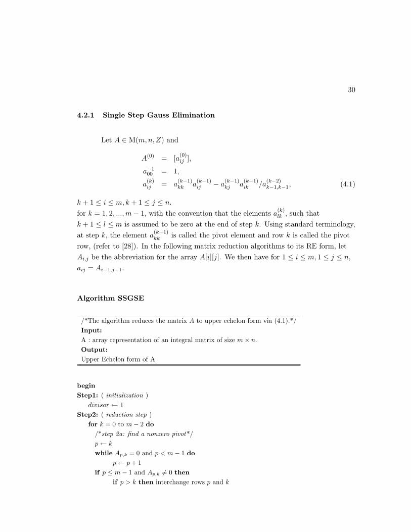
Let A ∈ M(m,n,Z) and

A(0) = [a(0)ij ],

a−100 = 1,

a(k)ij = a

(k−1)kk a

(k−1)ij − a

(k−1)kj a

(k−1)ik /a

(k−2)k−1,k−1, (4.1)

k + 1 ≤ i ≤ m, k + 1 ≤ j ≤ n.

for k = 1, 2, ...,m− 1, with the convention that the elements a(k)lk , such that

k + 1 ≤ l ≤ m is assumed to be zero at the end of step k. Using standard terminology,at step k, the element a

(k−1)kk is called the pivot element and row k is called the pivot

row, (refer to [28]). In the following matrix reduction algorithms to its RE form, letAi,j be the abbreviation for the array A[i][j]. We then have for 1 ≤ i ≤ m, 1 ≤ j ≤ n,aij = Ai−1,j−1.

Algorithm SSGSE

/*The algorithm reduces the matrix A to upper echelon form via (4.1).*/Input:A : array representation of an integral matrix of size m× n.Output:Upper Echelon form of A

beginStep1: ( initialization )

divisor ← 1Step2: ( reduction step )

for k = 0 to m− 2 do/*step 2a: find a nonzero pivot*/p ← k

while Ap,k = 0 and p < m− 1 dop ← p + 1

if p ≤ m− 1 and Ap,k 6= 0 thenif p > k then interchange rows p and k

31

/*step 2b: reduce so that the elements under pivot row in pivot column is zero*/for i = k + 1 to m− 1

for j = k + 1 to n− 1 doAi,j ← Ak,kAi,j −Ai,kAk,j/divisor

Ai,k ← 0divisor ← Ak,k

/*since p > m− 1, find pivot element in the next column*/end

4.2.2 Double Step Gauss Elimination

The two step fraction free scheme [28] is described.

a−100 = 1, (4.2)

a(0)ij = A(0), (4.3)

c(k−2)0 = a

(k−2)k−1,k−1a

(k−2)kk − a

(k−2)k−1,ka

(k−2)k,k−1/a

(k−3)k−2,k−2, (4.4)

c(k−2)i1 = a

(k−2)k−1,ka

(k−2)i,k−1 − a

(k−2)k−1,k−1a

(k−2)ik /a

(k−3)k−2,k−2, (4.5)

c(k−2)i2 = a

(k−2)k,k−1a

(k−2)ik − a

(i,k−1)kk a

(k−2)k−2 /a

(k−3)k−2,k−2, (4.6)

akij = c

(k−2)0 a

(k−2)ij + c

(k−2)i1 a

(k−2)kj + c

(k−2)i2 a

(k−2)k−1,j/a

(k−3)k−2,k−2, (4.7)

for 1 ≤ i ≤ m and 1 ≤ j ≤ n;

a(k−1)kk = c

(k−2)0 , (4.8)

a(k−1)kl = a

(k)kl

= a(k−2)k−1,k−1a

(k−2)kl − a

(k−2)k−1,l a

(k−2)k,k−1/a

(k−3)k−2,k−2, (4.9)

for k + 1 ≤ l ≤ n,

which is applied for k = 2, 4, ..., 2 ∗ floor(m− 1

2). When n is even, the last elimination

is performed by the single step method.

For the input matrix A = (aij) ∈ M(m,n,P(d)), let the vector valued functionrow be define such that row(i) = (ai+1,1, ..., ai+1,n) for each integer 0 ≤ i ≤ m− 1. Thealgorithm DSGSE is given as:

32

Algorithm DSGSE

/*The algorithm reduces the matrix A to upper echelon form via (4.7) and (4.9).*/Input: A: array representation of an integral matrix of size m× n.Output: Upper Echelon form of A

beginStep 1: divisor ← 1Step 2: (pivoting and reducing)

for (k = 1, k ≤ 2 ∗ floor(m− 1

2)− 1; k+ = 2)

Step 2a: (find a nonzero pivot) set q = 1Step 2b: set p = k

while p ≤ m− 1 doc0 ← Ak−1,k−1Ap,k −Ak−1,kAp,k−1/divisor

if c0 6= 0 then break(i.e goto Step 2c)else p ← p + 1

Step 2c:if p > m− 1 and k + q ≤ m− 1 then

interchange row k − 1 with row k + q

q ← q + 1goto Step 2b

Step 2d :if k + q > m− 1 then apply Algorithm SSGSE so that row k − 1 is the pivot rowStep 2e: (elements in columns k-1 and k below respective pivot row set to 0 )if c0 6= 0 and p ≤ m− 1 then

if p > k then interchange row k with row p

for i = k + 1 to i = m− 1 do (work on row k+1 to row m-1 )c1i ← Ak−1,kAi,k−1 −Ak−1,k−1Ai,k/divisor

c2i ← Ak,k−1Ai,k −Ak,kAi,k−1/divisor

for j = k + 1 to n− 1 doAi,j ← c0Ai,j + c1iAk,j + c2iAk−1,j/divisor

for j = k − 1 to k doset Ai,j = 0

for l = k + 1 to n− 1 do (work on row k)Ak,l ← Ak−1,k−1Ak,l −Ak−1,lAk,k−1/divisor

Ak,k−1 ← 0Ak,k ← c0; divisor ← Ak,k

end

33

4.2.3 The Rational Number Gauss Elimination

The Gauss elimination approach in the preceding section reduces an integralmatrix to its row echelon form by applying integer addition and multiplication andexact integer quotient, in order to preserve the integer entries of the echelon formmatrix. It is also possible to reduce a matrix over the rational number without firsttransforming the matrix to a row equivalent integer matrix but the complexity ofrational number arithmetic has to be applied. This approach shall not be omitted as itcan be regarded as a basis of comparison with the less complex algorithms involvingexact integer and modular arithmetic. The scheme for the rational number Gausselimination takes a naive approach in reducing the elements underneath the pivotelement to zero. Let A ∈ M(m,n, Z) be such that

A(0) = [a(0)ij ],

a(k)ij = a

(k−1)kk a

(k−1)ij − a

(k−1)kj a

(k−1)ik , (4.10)

k + 1 ≤ i ≤ m, k + 1 ≤ j ≤ n.

for k = 1, 2, ...,m− 1, with the convention that the elements a(k)lk such that

k + 1 ≤ l ≤ m is assumed to be zero at the end of step k as adopted by the single stepGauss elimination scheme whereby at step k, the element a

(k−1)kk is called the pivot

element and row k is called the pivot row.

Algorithm RNGSE

/*The algorithm reduces the matrix A to upper echelon form via (4.1).*/Input:A : array representation of an integral matrix of size m× n.Output:Upper Echelon form of A

begin

34

for k = 0 to m− 2 do/*step 1a: find a nonzero pivot*/p ← k

while Ap,k = 0 and p < m− 1 dop ← p + 1

if p ≤ m− 1 and Ap,k 6= 0 thenif p > k then interchange rows p and k

/*step 1b: reduce so that the elements under pivot row in pivot column is zero*/for i = k + 1 to m− 1 do

for j = k + 1 to n− 1 doAi,j ← Ak,kAi,j −Ai,kAk,j

Ai,k ← 0/*since p > m− 1, find pivot element in the next column*/

end

4.3 On the Nonmodular OPBGCD Algorithms

From the general algorithm of 3.4, a general nonmodular algorithm for theexact computation of the GCD of two polynomials relative to an orthogonal basis isdescribed.

Algorithm OPBGCD (Orthogonal-Basis Polynomial GCD)

Input:α = (α0, ..., αn−1), β = (β0, ..., βn−1) and γ = (γ0, ..., γn−1).The polynomials, a = (a0, a1, ..., an−1, 1), b = (b0, b1, ..., bm, ..., bn−1).h = n− 1.Output:The monic generalized polynomial c = gcd(a, b) of degree k.

beginStep1: ( Calculation of the comrade matrix )

CMR ← CDEMOFP(α, β, γ, a, b, n− 1)

Step2: ( Calculation of the systems coefficient matrix )

35

CSY S ← CSFCDEM(α, β, γ, b, CMR, n− 1)

Step3: ( Find RE form of CSY S and solution to GCD of a and b )

Step4: output(solution)end

Algorithm OPBGCD can be modified by the application of a differenttechnique in reducing the array representation of the matrix CSY S obtained fromstep 2, to its row echelon form. This leads to the construction of 3 differentnonmodular algorithms, namely the OPBGCD-SSGSE, OPBGCD-DSGSE and theclassical OPBGCD-RNGSE algorithms. The algorithms derived its name from thethree different matrix reduction techniques described in 4.2. In the followingdiscussion, we describe the subalgorithm SSGSE-SOLN, which is the subalgorithmcalled in step 3 of OPBGCD-SSGSE algorithm. The other two algorithms, namely theOPBGCD-DSGSE and OPBGCD-RNGSE calls the DSGSE-SOLN algorithm andRNGSE-SOLN algorithm respectively, which are extensions of the DSGSE andRNGSE algorithms respectively. The reduction algorithms are extended in order tocompute the coefficients of the GCD from the RE form of the reduced matrix.

Algorithm SSGSE-SOLN

/*The algorithm reduces the matrix A to upper echelon form via (4.1)and computes gcd(a, b)*/Input:A : array representation of an integral matrix of size m× n.Output:c = gcd(a, b) such that ci ∈ Q.

beginStep1: ( initialization )

divisor ← 1Step2: ( reduction step )

for k = 0 to m− 2 do/*step 2a: find a nonzero pivot*/

36

p ← k

while Ap,k = 0 and p < m− 1 dop ← p + 1

if p ≤ m− 1 and Ap,k 6= 0 thenif p > k then interchange rows p and k

/*step 2b: reduce so that the elements under pivot row in pivot column is zero*/for i = k + 1 to m− 1 do

for j = k + 1 to n− 1 doAi,j ← Ak,kAi,j −Ai,kAk,j/divisor

Ai,k ← 0divisor ← Ak,k

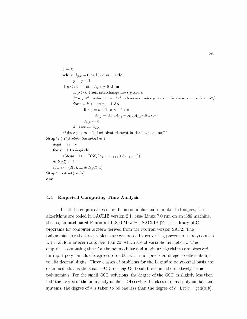
/*since p > m− 1, find pivot element in the next column*/Step3: ( Calculate the solution )

degd ← n− r

for i = 1 to degd dod(degd− i) ← RNQ(Ar−1,r−1+i, (Ar−1,r−1))

d(degd) ← 1isoln ← (d(0), ..., d(degd), 1)

Step4: output(isoln)end

4.4 Empirical Computing Time Analysis

In all the empirical tests for the nonmodular and modular techniques, thealgorithms are coded in SACLIB version 2.1, Suse Linux 7.0 run on an i386 machine,that is, an intel based Pentium III, 800 Mhz PC. SACLIB [22] is a library of Cprograms for computer algebra derived from the Fortran version SAC2. Thepolynomials for the test problems are generated by converting power series polynomialswith random integer roots less than 20, which are of variable multiplicity. Theempirical computing time for the nonmodular and modular algorithms are observedfor input polynomials of degree up to 100, with multiprecision integer coefficients upto 153 decimal digits. Three classes of problems for the Legendre polynomial basis areexamined; that is the small GCD and big GCD solutions and the relatively primepolynomials. For the small GCD solutions, the degree of the GCD is slightly less thenhalf the degree of the input polynomials. Observing the class of dense polynomials andsystems, the degree of b is taken to be one less than the degree of a. Let c = gcd(a, b).

37

4.4.1 Computing Time for OPBGCD-SSGSE and OPBGCD-DSGSE

The timing results (in seconds) for the OPBGCD-SSGSE andOPBGCD-DSGSE for the three classes of problems are tabulated below:

Table 4.1: Timing Results (in secs) for the Legendre Polynomial Basis: Small GCD Case

deg(a) deg(c) OPBGCD-DSGSE OPBGCD-SSGSE

20 3 0.23 0.29

40 15 10.44 14.22 (+N2000000)

60 25 133.96 (+N2000000) 197.68 (+N2000000)

80 38 599.48 (+N4000000) 975.20 (+N4000000)

100 38 3859.00 (+N8000000) -

Table 4.2: Timing Results (in secs) for the Legendre Polynomial Basis: Big GCD Case

deg(a) deg(c) OPBGCD-DSGSE OPBGCD-SSGSE

20 16 0.06 0.06

40 33 1.11 1.11

60 54 3.13 3.89

80 72 13.93 19.81

100 85 134.00 (+N4000000) 170.61 (+N4000000)

Remark: In the above results, +N2000000 allocates an additional two million wordsof memory to list storage. If no memory allocation is written, +N1000000 words ofmemory to list storage have been used, which is the allocation by default.

From the empirical results in Table 4.1, the ratio of the average computing time forOPBGCD-SSGSE to OPBGCD-DSGSE is approximately equals to 1.6. The ratio ofthe average computing time of OPBGCD-SSGSE to OPBGCD-DSGSE for the bigGCD case is reduced to about 1.3. The performance of OPBGCD-DSGSE for thethree different class of problems is shown in Table 4.4.

38

Table 4.3: Timing Results (in secs) for the Legendre Polynomial Basis: Relatively Prime Case

deg(a) OPBGCD-DSGSE OPBGCD-SSGSE

20 0.34 0.43

40 46.4 (+N2000000) 67.80 (+N2000000)

60 197.5 (+N2000000) 300.78 (+N2000000)

80 1884.00 (+N4000000) -

Table 4.4: OPBGCD-DSGSE Timing Results (in secs) for the Legendre Polynomial Basis

deg(a) small GCD big GCD relatively prime

20 0.23 0.06 1.00

40 10.44 1.11 46.4

60 133.96 3.13 197.5

80 599.48 13.93 1884.00

100 3859.00 134.00 -

4.5 Discussions

The empirical results emphasize the superiority of OPBGCD-DSGSE overOPBGCD-SSGSE. The results correspond to the superiority of the double step Gausselimination algorithm which is about twice the efficiency of the single step Gausselimination algorithm. As a comparison in the performance of OPBGCD-DSGSEalgorithm between the three different class of problems, the results show that for afixed degree of the polynomial inputs a, the algorithm takes the shortest time in thebig GCD case, when the rank of the corresponding systems coefficient matrix is smallin size. In other words, for same degree inputs, the execution time for the relativelyprime case (rank=n = deg(a)) is greater than the small GCD case (big rank butsmaller than n) which is in fact also greater than the big GCD case (small rank).

39

CHAPTER V

A MODULAR GENERALIZED POLYNOMIAL GCD COMPUTATION

5.1 An Introduction to the Modular Approach

The following discussion is based on the theories that have been established inBarnett [7] and [11]. Consider the situation when the polynomials a(x) and b(x) are inthe generalized form (1.4), such that the degree of a is greater than or equal to degreeof b. We refer to the general algorithm described in 3.4 involving the comrade matrixapproach which comprises of:

1. constructing the comrade matrix (3.3) associated with a(x).

2. applying the recursive equation (3.11) to construct the systems of linearequations described in 3.3.1.

3. reducing the coefficient matrix in step 2 to upper echelon form and finding thedesired solution.

From the procedure described above, it is observed that the incorporation ofthe modular technique is possible at 3 different stages, that is either from the stage ofthe construction of the comrade matrix at step 1 onwards, or from the application ofthe recursive equation at step 2 onwards, or solely from step 3 which reduces thematrix obtained from step 2 (which may include multiprecision integer entries) to itsrow echelon form followed by the computation of the coefficients of the GCD. Theapplication of the modular approach computes the solution to the GCD in severalfinite fields which eventually converges to the true solution when the bound for thesolution has been exceeded. The method involves the application of 2-congruenceChinese remainder algorithm (CRA) followed by the rational number reconstructionalgorithm (RNRA), since the true solution is in the form of a monic generalized

40

polynomial with rational number coefficients. In this Chapter, we present a modulartechnique that applies modular arithmetic only at step 3, that is, in the Gausselimination procedure on a matrix A (mod pi) followed by the computation of thesolution gcd (mod pi), for i = 1, ..., n for some n.

The algorithm MOPBGCD in [2] suggests a termination test that caneliminate the application of unlucky primes. The algorithm [2] has not been tested forpolynomials with multiprecision coefficients. A complete form of the application of themodular approach is presented in the following algorithm.

41

5.2 Algorithm MOPBGCD

Input:The defining terms αi, βi and γi for 0 ≤ i ≤ n− 1.The generalized polynomial, a = (a0, a1, ..., an−1, 1).The generalized polynomial b = (b0, b1, ..., bm, ..., bn−1), m ≤ n.Output:The monic generalized GCD c such that c = gcd(a, b) is of degree k.

beginStep1: ( Calculation of the comrade matrix )

CMR ← CDEMOFP(α, β, γ, a, b, n− 1)

Step2: ( Calculation of the systems coefficient matrix )CSY S ← CSFCDEM(α, β, γ, b, CMR, n− 1)

Step3: ( Initialization )set k = 1 and set n = 1

Step4: ( Chinese remainder algorithm )find a prime p0 and the matrix CSY S (mod p0)find the reduced matrix and the solution C0 in Zp0

if deg(C0) = 0 then output(1)set pnew = p0 and set Cnew = C0

Step5:Step 5a:set k = k + 1find a prime p0 and the matrix CSY S (mod p0)find the reduced matrix and the solution C0 in Zp0

if deg(C0) > deg(Cnew) then(p0 is unlucky. Find another prime)set k = k − 1; goto Step5

else if deg(C0) < deg(Cnew) then(all previous primes unlucky)set k = 1; n = 1; goto step4

Step 5b:Solve for the 2-congruence CRA :

C1∼= C0 (mod p0) and C1

∼= Cnew (mod pnew)set Cnew = C1 and set pnew = p0 ∗ pnew

if k ≤ 2n then goto step5

Step6: ( rational number reconstruction )

42

Step7: ( if rational reconstruction fails )set n = n + 1; goto step5

Step8: ( divisor test and preparing output )if test true then output( solution )else

if there is still enough primes thenset n = n + 1 and goto Step 5

else (the primes are exhausted)output( all primes were unlucky )

end

In short, CSFCDEM applies a recursive equation involving the defining termsand the comrade matrix resulting as the matrix coefficient of a certain systems ofequations. This rational number matrix coefficient obtained from the recursiveequations is transformed into an equivalent integral matrix CSY S, which is returnedby CSFCDEM. In this approach, steps 1 and 2 applies rational number andmultiprecision integer arithmetic operations.

5.2.1 The Selection of Primes

The MOPBGCD requires a list of distinct odd single precision primes. The listcan be generated by the application of SACLIB’s function DPGEN(m, k) so that theprime pi in the list is such that m ≤ pi < m + 2k. SACLIB2.1 also provides such a listcalled LPRIME. The list LPRIME is used in the MOPBGCD algorithm and is suchthat LPRIME = {536830337, ..., 536870909}. There are 2055 elements in this listwhere each prime pi is nearly as large as the maximum single precision integer.MOPBGCD calls for the subroutine FDPRIME which calls for LPRIME(i), the ithelement of LPRIME. For each row 1 ≤ i ≤ n of the matrix A obtained from thesubroutine CSFCDEM, the element aij of each column 1 ≤ j ≤ n is converted to aij

(mod pi) ∈ GF(pi) by applying SACLIB’s function MDHOM. If there exists a singlerow such that all the column elements (mod pi) are equal to 0, the process of takingthe homomorphic images is terminated and a new prime is selected. The wholeprocedure is then repeated until there is no single row whose column elements are all

43

divisible by the selected prime. A (mod pi) is thus obtained and applied to thesubroutine MGSEGCD. By this technique we are able to simultaneously check thatthe homomorphic images of the elements of A does not alter the rank of the matrix A.

5.2.2 Finding the Row Echelon Form and Solution in GF(p)

The algorithm reduces the matrix A (mod p) to upper echelon form in GF(p)and computes the coefficients of the GCD in GF(p).

Algorithm MGSEGCD

Input:A : array representation of an m× n matrix in GF(p).Output:isoln = (d(0), ..., d(deg(d)), 1), the coefficients of gcd(a, b) (mod p).

beginStep 1: ( reduction step )

for k = 0 to m− 2 do/*step 1a: find a nonzero pivot*/p ← k

while Ap,k = 0 and p < m− 1 dop ← p + 1

if p ≤ m− 1 and Ap,k 6= 0 thenif p > k then interchange rows p and k

/*step 1b: reduce so that the elements under pivot row in pivot column is zero*/for i = k + 1 to m− 1 do

for j = k + 1 to n− 1 doAi,j ← (Ak,k ∗Ai,j −Ai,k ∗Ak,j) (mod p)

Ai,k ← 0/*since p > m− 1, find pivot element in the next column*/

Step2: calculate the rank r of AStep3: ( calculate the solution (mod p))

degd ← n− r

for i = 1 to degd dod(degd− i) ← Ar−1,r−1+i ∗ INV(Ar−1,r−1) (mod p)

d(degd) ← 1

44

isoln ← (d(0), ..., d(degd), 1)Step4: output(isoln) end

The computation of Ai,j (mod p) ← (Ak,k ∗Ai,j −Ai,k ∗Ak,j) (mod p) at step 1bapplies SACLIB’s function MDSUM, MDNEG and MDPROD which computes thesum, negative and product of elements in GF(p) for single precision prime p. Let A bethe RE form of the matrix obtained from step 1. The rank of A can be calculated bychecking if aij is 0, for each i from m to 1 and for each column 1 ≤ j ≤ n. If ars forsome s, is the first nonzero element encountered, then rank of A is r. Obviously, sinceall the computations in GF(p) is of order 1, the computing time of step 1 is dominatedby m2n. The computation of the rank is dominated by mn and the computation ofthe solution is dominated by degd ¹ n. If m = n then tMGSEGCD ¹ n3.

5.2.3 The Application of CRA to MOPBGCD Algorithm

Step 5 of algorithm MOPBGCD dominates the cost of applying the Chineseremainder algorithm. Let γ be the number of good primes used. Assuming that all theprimes are of good reduction, we compute the cost of the (k − 1)st iteration of theCRA as follows:

1. if |CSY S|∞ then the cost of computing CSY S (mod pk) is dominated byn2L(C).

2. The cost of finding the solution ck (mod pk) where

ck (mod pk) = (dk,0 (mod pk), dk,1 (mod pk), ..., dk,δ (mod pk))

is the cost of applying algorithm MGSEGCD which is dominated by n3 + δ.

3. Let Ck be the solution to the (k − 1)st iteration of the CRA. The cost ofcomputations in step 5b is the cost of solving the 2-congruence CRA given by

c ∼= ck (mod pk),

c ∼= Ck−1 (mod Pk−1),

45

such that Ck−1 is the solution modulo Pk−1 = p1p2...pk−1 obtained from the(k − 2)st iteration. Ck is obtained by solving

xk−1 = INV(Pk−1 (mod pk), pk)(ck − Ck−1 (mod pk)) (mod pk),

Ck = Ck−1 + xk−1Pk−1. (5.1)

The cost of computing xk−1 is dominated by L(Pk−1). Now,

Ck−1 = x0 + p1x1 + ... + p1p2...pk−2xk−2

≤ p1 − 1 + p1(p2 − 1) + ... + p1p2...(pk−1 − 1)

= Pk−1,

which implies that the computing time for computing Ck for the (k − 1)stiteration of the CRA is dominated by L(Pk−1). Since each xk−1 and Ck of (5.1)has δ terms, the cost of computing these terms is dominated by δL(Pk−1)

Therefore the cost of computing step 5, if γ primes are used is such thatt5 ¹ γ(n2L(C) + n3 + δL(p1p2...pγ)).

Let a and b be in the generalized form such that gcd(a, b) = d and|num(di)| < D, 0 < den(di) < D. Let n1 be number of primes of good reduction used.

Then, D <√

M2 such that M = p1...pn1 . From M > 2D2 and taking the least possible

prime, i.e pi = 2, we have 2n1 > 2D2 ⇔ n1 > 1 + 2log2(D). So, if p > 2 thenn1 ≤ 2 log2(D) + 2 ∼ log2(D). The total cost of applying the CRA is dominated bylog2(D)(n2L(C) + n3 + δL(M)) such that M = p1p2...plog2(D), that is when takingγ = log2(D).

5.2.4 The Rational Number Reconstruction Algorithm

Given u ∈ GF(M) such that M is the product of several primes, the algorithmfinds the integers a and b that satisfies a ∼= ub (mod M) and outputs a solution if itexists or outputs NIL if the solution does not exist. MOPBGCD applies SACLIB’sfunction RNFMR to reconstruct rational numbers from the coefficients of the GCDwhich is an output of MILLCRA obtained in GF(M). If the number of primes

46

composing M is not sufficient, we abort the attempt to find the rest of the coefficientsof the GCD. It can be shown that shown that the computing time for the classicalrational number reconstruction algorithm, given that u ∈ GF(M) is dominated byL(u)L(M) + L2(M). If the degree of GCD d is δ then the total cost for each executionis dominated by δL2(M).

If k is the number of times that the rational number reconstruction algorithm isattempted, that is for every 2k + 1, we therefore have k ¹ log2(log2(D)). The totalcost of applying the RNRA to obtain a correct solution if all the n1 primes are lucky isdominated by δ log2(log2(D))L2(M). In this case, the computing time for theapplication of CRA and RNRA algorithms is dominated by

log2(D)(n2L(C) + n3 + δL(M)) + δ log2(log2(D))L2(M)

¹ L(D)(n2L(C) + nL2(M) + n3)

¹ n3L(D)(L(C) + L2(M))

such that M = p1p2...pL(D). Note that log2(D) ≤ log2(D) + 1 ∼ L(D).

5.2.5 The Termination Criterion

Once the function RNFMR returns a polynomial with all of its coefficientshaving a solution, MOPBGCD applies a divisor test to check if the candidate solutiondivides each of the input polynomial. Let gcd(a, b) = d such that deg(d) = δ. TheOPDIV algorithm described in the preceding chapter generates the generalizedpolynomial remainder sequence (a = r0, r1, ..., rk+1), in which ri+1 is the remainderwhen ri is divided by xdeg(ri)−δ ∗ d and r0 = a. Assuming classical matrixmultiplication, the cost of obtaining the deg(ri) + 2 components of xdeg(ri)−δ ∗ d,comprising the coefficients of the remainder is dominated by deg(ri)3 ¹ n3. Summingup the cost for 1 ≤ i ≤ n− δ gives a total cost that is dominated by n3. We thereforeclaim in ?? that OPDIV is quartic in n, where n is the degree bound of the inputpolynomials. However, further work will be required for finding the computing timebound in terms of the parameters of its input variables.

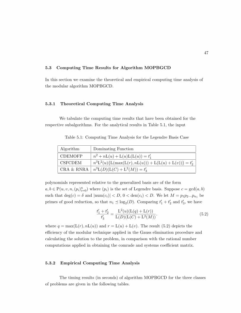
47

5.3 Computing Time Results for Algorithm MOPBGCD

In this section we examine the theoretical and empirical computing time analysis ofthe modular algorithm MOPBGCD.

5.3.1 Theoretical Computing Time Analysis

We tabulate the computing time results that have been obtained for therespective subalgorithms. For the analytical results in Table 5.1, the input

Table 5.1: Computing Time Analysis for the Legendre Basis Case

Algorithm Dominating Function

CDEMOFP n2 + nL(u) + L(u)L(L(u)) = t′1CSFCDEM n3L2(u){L(max(L(r), nL(u))) + L(L(u) + L(v))} = t′2CRA & RNRA n3L(D)(L(C) + L2(M)) = t′3

polynomials represented relative to the generalized basis are of the forma, b ∈ P(u, v, n, (pi)n

i=0) where (pi) is the set of Legendre basis. Suppose c = gcd(a, b)such that deg(c) = δ and |num(ci)| < D, 0 < den(ci) < D. We let M = p1p2...pn1 beprimes of good reduction, so that n1 ¹ log2(D). Comparing t′1 + t′2 and t′3, we have

t′1 + t′2t′3

=L2(u)(L(q) + L(r))

L(D)(L(C) + L2(M)). (5.2)

where q = max(L(r), nL(u)) and r = L(u) + L(v). The result (5.2) depicts theefficiency of the modular technique applied in the Gauss elimination procedure andcalculating the solution to the problem, in comparison with the rational numbercomputations applied in obtaining the comrade and systems coefficient matrix.

5.3.2 Empirical Computing Time Analysis

The timing results (in seconds) of algorithm MOPBGCD for the three classesof problems are given in the following tables.

48

Table 5.2: MOPBGCD for the Legendre Polynomial Basis: Small GCD Case

deg(a) deg(c) maxdigit{ai, bi} execution time (secs) no. of primes memoryMOPBGCD

20 3 30 0.07 3 default

40 15 59 0.68 5 default

60 25 88 3.09 9 default

80 38 113 9.07 17 default

100 38 153 17.7 17 +N2000000

Table 5.3: MOPBGCD for the Legendre Polynomial Basis: Big GCD Case

deg(a) deg(c) execution time (secs) no. of primes memoryMOPBGCD

20 16 0.06 5 default

40 33 0.86 17 default

60 54 3.68 33 default

80 72 8.74 33 default

100 85 19.77 33 +N2000000

As in 4.4.1, +N2000000 allocates an additional two million words of memory tolist storage. The default allocation is 1000000 words. As expected, the big GCD caserequires more primes and execution time compared to the small GCD case. For a fixeddegree of the polynomials tested, although the number of primes required for the bigGCD case is about twice that of the small GCD case, the differences in computingtime or space required in the two cases is not so significant. For the relatively primecase, the program terminates upon encountering a solution c such that deg(c) = 0,since the degree of the actual solution cannot be any smaller. Unless a bad prime isencountered before this actual solution is obtained, in which case, the rank of thesystems coefficient matrix is less than n, the number of primes used will be equal to 2.Therefore, the relatively prime case may be expected to consume the shortest time,assuming that the first encounter is a good prime. The theoretical computing time

49

Table 5.4: MOPBGCD for the Legendre Polynomial Basis: Relatively Prime Case

deg(a) execution time (secs)MOPBGCD

20 0.07

40 1.06

60 1.83

80 6.49

Table 5.5: MOPBGCD Timing Results in secs for the Legendre Polynomial Basis

deg(a) small GCD big GCD relatively prime

20 0.07 0.06 0.07

40 0.68 0.86 1.06

60 3.09 3.68 1.83

80 9.07 8.74 6.49

100 17.77 19.74 -

results of the preceding section, compares the computing time required by the rationalnumber algorithms (in steps 1 and 2 of 3.4), to the modular algorithm which appliesthe CRA and RNRA algorithms prior to the application of the divisor test OPDIValgorithm. The empirical results of the test problems were obtained so that empiricalcomparisons can be made with respect to this application.

5.4 Discussions

Table 5.2, 5.3 and 5.4 respectively, presents the total execution time ofMOPBGCD with respect to 3 classes of problems described in 4.4. For a fixed degreeinput of the test problems, the sum of the execution time of the subalgorithms ofMOPBGCD in columns 3 and 4 of Table 5.6 and 5.7, respectively, is subtracted fromthe total execution time for the problem to obtain the respective execution time forOPDIV. The efficiency of OPDIV with respect to MOPBGCD is clearly indicatedfrom the timing results of the last columns of Tables 5.6 and 5.7. Moreover, Table 5.6

50

Table 5.6: Execution time in secs : MOPBGCD sub-algorithms for Small GCD Legendre BasisInputs

deg(a) deg(c) Rational Arithmetic Modular arithmetic OPDIV

20 3 0.04 0.01 0.01

40 15 0.4 0.13 0.15

60 25 1.62 0.84 0.63

80 38 3.87 3.81 1.39

100 38 7.52 7.40 2.78

Table 5.7: Execution time in secs : MOPBGCD sub-algorithms for Big GCD Legendre BasisInputs

deg(a) deg(c) Rational Arithmetic Modular arithmetic OPDIV

20 16 0.04 0.01 0.01

40 33 0.42 0.31 0.13

60 54 1.52 2.00 0.16

80 72 3.74 4.68 0.32

100 85 8.09 10.70 0.98

shows that the execution time for the application of rational number arithmetic insteps 1 and 2 of 3.4 exceeds the execution time for the application of modulararithmetic of the succeeding steps, only when the size of the GCD is sufficiently small.When the size of the GCD is sufficiently big, the modular approach of reducing thesystems coefficient matrix to its RE form and computing the rational number solutionis as time consuming as the application of the rational number arithmetic of thepreceding steps. A hybrid of these two approaches can be of advantage to thealgorithm, whereby the rational number functions were already made available.

51

CHAPTER VI

SUMMARY, CONCLUSIONS AND FURTHER RESEARCH

6.1 Introduction

We now reflect on what have been the results of this research, summarizing ourfindings and suggesting areas for further investigations. The main goal of this study isto produce a useful tool for computing the GCD of polynomials in the generalizedform such that the general basis satisfies the three term recurrence relation. In theempirical comparisons, we study the performance of the algorithms on polynomialsrepresented relative to an orthogonal basis, which are a special class of thepolynomials in the general basis.

6.2 Significant Findings and Conclusions

The initial task of the work is to construct and implement the nonmodularalgorithms from a general OPBGCD algorithm. This is achieved by the constructionof the algorithms for constructing the comrade matrix of a polynomial (AlgorithmCDEMOFP) and the coefficient systems for the comrade matrix (AlgorithmCSFCDEM). This algorithms apply SACLIB’s rational number or multiprecisioninteger arithmetics. Auxiliary algorithms for matrix computations have also beenconstructed and included in the appendix. The auxiliary algorithms are called by thecomrade matrix and coefficient systems algorithms.

The modular techniques have been known for its competitiveness in dense classof problems related to the GCD and matrix related problems such as finding thedeterminants or solutions to linear equations. Therefore, it is our objective toemphasize the superiority of the implementation of the modular techniques in ouralgorithms, focusing only at the class of dense polynomials with multiprecision

52

coefficients in our empirical inputs.

According to [43], the small GCD class of power series polynomials is known tobe the worst case for the Euclidean algorithm but is usually the best case for themodular algorithms. In the case of computing the GCD of polynomials in thegeneralized form, the modular techniques that have been developed are especiallyappreciated for being markedly superior then the nonmodular techniques for the classof dense rational number polynomials with small GCD solutions. The empiricalcomputing time results show that the modular algorithms are markedly superior tothe nonmodular algorithms when the polynomials are sufficiently dense with degree atmost 100, the numerators of the coefficients at most 153 digits and the magnitude ordegree of the GCD is about less than half the degree of the input polynomials (smallGCD case). In this case, the modular algorithms are on the average about 60 timesfaster than the nonmodular algorithms.

The empirical time results also suggest that a hybrid application of themodular approach and multiprecision arithmetic can be regarded as efficient for boththe small and big GCD solutions such that the bound of the true GCD solution arenot predetermined, provided also that a correct solution can be acquired from thetechnique.

The efficiency of the modular approach requires efficient integration andimplementation of the devisor test and rational number reconstruction algorithms.The divisor test acts as a termination criterion that can also determines theeffectiveness of the method. A bad prime p is encountered if p divides the leadingcoefficient of the input polynomials or p divides the entries of the last row of the REform of the equivalent integral systems coefficient matrix. Thus, the divisor test is anessential device that determines the correctness of the final solution and eliminates theuse of a bad reduction.

Given two polynomials in its generalized form, the polynomials can beconverted to its power series form for the GCD computations and converted back toits generalized form. The transformation from a polynomial in the generalized form toa polynomial in the power series form requires multiplication of an (n + 1)× (n + 1)matrix with and n + 1 column vector and is therefore of magnitude O(n2). The

53

transformation of a polynomial in the power series representation to a polynomial inthe general basis representation requires finding the unique solution to an n× n

systems of equations, which is roughly O(n3). The application of the Gausselimination algorithm is basically O(n3) with the coefficient of n3 determined by thelength of multiprecision integers involved in the computation. The contribution of theresearch into constructing and implementing an effective and efficient OPBGCDalgorithms is not a trivial one. With the results of this research, the applications ofthe exact Gauss elimination methods (modular or nonmodular) have also beenextended to the exact computations of the GCD of generalized polynomials.

6.3 Future Research

The empirical computing time results in the preceding chapter also illustratethe efficiency of the modular technique in computing the GCD of 2 polynomialsrelative to the Legendre basis. The computing time takes only seconds when thedegree bound for the input polynomial is 100 and the coefficient bound 153 decimaldigits. With the value of the defining terms dependent on the degree bound, so thatthese values remain single precision, we are able to construct an efficient algorithm forcalculating the comrade and systems coefficient matrix using classical rational numberarithmetic and devote the application of the modular technique to the Gausselimination procedure, which is then followed by the computations of the integersolution to the problem in simpler domains and finding the rational number solutionin the original domain. We will work on the extension of the application of themodular technique to further reduce the number of multiprecision computations andthe rational number arithmetic involved in steps 1 and 2 of the general algorithm in3.4. However, further properties of the homomorphic image scheme have to becarefully investigated to enable the application of the modular technique in theconstruction of the comrade and the systems coefficient matrices.

54

BIBLIOGRAPHY

[1] Ali A. Rahman(1992). “The Use of GCD Computation to Remove RepeatedZeroes from a Floating Point Polynomial.” SCAN92 Conference. Oldenberg,Germany.

[2] Ali Abdul Rahman and Nor’aini Aris(2001). “Alkhwarizmi Modulo PembahagiSepunya Terbesar Dua Polinomial Relatif Terhadap Asas Berortogon.”Simposium Kebangsaan Sains Matematik ke-9, Julai 2001 UKM, Bangi, Malaysia.

[3] Ali Abdul Rahman and Nor’aini Aris(2002). “The State of the Art in ExactPolynomial GCD Computations.” MSTC 2002. Symposium A: Physical SciencesEngineering and Technology. 19-21 September 2002. Johor Bahru, Malaysia.

[4] Bareiss, E.H.(1968). “Sylvester’s identity and Multistep Integer PreservingGaussian Elimination.” Math.Comp. 22(103). 565-578.

[5] Bareiss, E.H.(1972). “Computational Solutions of Matrix Problems over anIntegral Domain.” J. Inst. Math. Applic. 10. 68-104.

[6] Barnett, S.(1975). “A Companion Matrix Analogue for Orthogonal Polynomials.”Linear Algebra and its Applications. 12. 197-208.

[7] Barnett, S. and Maroulas, J.(1978). “Greatest Common Divisor of GeneralizedPolynomial and Polynomial Matrices.” Linear Algebra and its Applications. 22.195-210.

[8] Barnett, S. and Maroulas, J.(1979). “Polynomials with Respect to a GeneralBasis. I. Theory.” J. of Math. Analysis and Applications. 72. 177-194.

55

[9] Barnett, S. and Maroulas, J.(1979). “Polynomials with Respect to a GeneralBasis. II. Applications.” J. of Math. Analysis and Applications. 72. 599-614.

[10] Barnett, S. and Maroulas, J.(1979). “Further Results on the Qualitative Theoryof Generalized Polynomial.” J. Inst. Maths Applics. 23. 33-42.

[11] Barnett, S.(1983). “Polynomials and Linear Control Systems.” New York andBasel:Marcel Dekker.

[12] Borosh, I., Fraenkel, A.S.(1966). “On Modular Approaches to Solving Systems ofLinear Equations with Rational Coefficients.” Math.Comp. 20. 107-112.

[13] Brown, W.S.(1971). “On Euclid’s Algorithm and Polynomial Greatest CommonDivisors.” J. ACM. 18(1). 478 - 504.

[14] Brown, W.S. and Traub, J.F.(1971). “On Euclid’s Algorithm and the Theory ofSubresultants” J. ACM. 18, 1971.

[15] Cabay, S.(1971). “Exact Solution of linear Equations.” Proc. Second Symp. onSymbolic and Algebraic Manipulation, ACM, New York. 392 - 398.

[16] Cabay, S. and Lam, T.P.L.(1977). “Congruence Techniques for the Exact Solutionof Integer Systems of Linear Equations.” ACM TOMS. 3(4). 386-397.

[17] Cabay, S. and Lam, T.P.L. (1977). “Algorithm 523, ESOLVE: CongruenceTechnique for the exact solution of integer systems of linear equations.” ACMTrans. Math. Software 3(4). (Dec. 1977). 404 - 410.

[18] Collins, G.E.(1967). “Subresultants and Reduced Polynomial RemainderSequences.” J. ACM. 14(1).

[19] Collins, G.E.(1971). “The Calculation of Multivariate Polynomial Resultants.” J.ACM. 18(4) (Oct.1971). 144-152.

[20] Collins, G.E.(1974). “The Computing Time of the Euclidean Algorithm.” SIAMJournal on Computing. 3(1). 1-10.

[21] Collins, G.E., Mignotte, M and Winkler, F.(1982). “Arithmetic in Basic AlgebraicDomains.” Computing Suppl. 4. 189-220.

56

[22] Collins, G.E. et al.(1993). “SACLIB1.1 User’s Guide.” Research Institute forSymbolic Computation, Johannes Kepler University: RICS-Linz Report SeriesTechnical Report Number 93-19.

[23] Collins, G.E. and Encarnacion, M.J.(1995). “Efficient Rational NumberReconstruction.” J.Symbolic Computation. 20, 287 - 297.

[24] Char, B.W., Geddes, K.O. and Gonnet, G.H.(1989). “GCDHEU: HeuristicPolynomial GCD Algorithm Based on Integer GCD Computation.” J. SymbolicComput. 7. 31-48.

[25] Davenport J.H.(1987). “How Elementary Upper Bounds Generate CheaperData.” in Caviness,B.(ed): Proc. EUROCAL. 2.

[26] Davenport, J.H., Siret,Y. and Tournier, E.(1988). “Computer Algebra: Systemsand Algorithms for Algebraic Computation.” London:Academic Press.

[27] Encarnacion, M.J.(1994). “On a Modular Algorithm for Computing GCDs ofpolynomials over Algebraic Number Fields.” in Von Zur Gathen, J. andGiesbrecht, M.(eds): Proceedings of the International Symposium on Symbolicand Algebraic Computation. ACM, New York. 58 - 65.

[28] Geddes, K.O., Czapor, S.R. and Labahn.(1992). “Algorithms for ComputerAlgebra.” , Boston: Kluwer Academic Publishers.

[29] Grant, J.A. and Rahman, A.A.(1992). “Determination of the zeros of a linearcombination of generalised polynomials.” J. of Computational and AppliedMathematics. 42. 269-278.

[30] Howell, J.A. and Gregory, R.T.(1969). “An Algorithm for Solving LinearAlgebraic Equations Using Residue Arithmetic.” BIT. 9. 200-234. 324-337.

[31] Howell, J.A.(1971). “Algorithm 406: Exact Solutions of Linear Equations UsingResidue Arithmetic.” Comm. ACM. 14, 3 (March 1971). 180-184.

[32] Jebelean, T.(1993). “Improving the Multi-Precision Euclidean algorithm.” inProceedings of DISCO ’93.

57

[33] Langemyr, L.(1989). “Computing the GCD of two Polynomials over an AlgebraicNumber Field.” The Royal Institute of Technology, Stockholm, Sweden: Ph.D.Thesis.

[34] Lauer, M.(1982). “Computing by Homomorphic Images.” in Buchberger, B.,Collins, G.E. and Loos,R.(eds) in cooperation with Albrecht, R: ComputerAlgebra Symbolic and Algebraic Computation, Computing Suppl. 4. New York:Springer Verlag. 139-168.

[35] Lipson, J.D.(1981). “Elements of Algebra and Algebraic Computing.” MenloPark, California: Benjamin/Cummings. Publishing Company.

[36] Kaltofen, E. and Monagan, M.B.(1999). “On the Genericity of the ModularPolynomial GCD Algorithms.” J. ACM. 59-65.

[37] Knuth, D.E.(1981). “The Art of Computer Programming. vol II.” Reading, Mass:Addison Wesley.

[38] Mazukelli, D.(1972). “Multistep Elimination over Commutative Rings.”Northwestern University, Illinois: Ph.D. Thesis.

[39] McClellan, M.T.(1971). “The Exact Solution of Systems of Linear Equations withPolynomial Coefficients.” U. of Wisconsin, Madison, Wis: Ph.D. Thesis.

[40] McClellan, M.T.(1973). “The Exact Solution of Systems of Linear Equations withPolynomial Coefficients.” J.ACM. 20(4). 563-588.

[41] McClellan, M.T.(1977). “A Comparison of Algorithms for the Exact Solution ofLinear Equations.” ACM Trans Math Software. 3(2). 147-158.

[42] Mohamed Omar Rayes(1995). “Parallel Integral Multivariate Polynomial GreatestCommon Divisor Computation.” Kent State University: Ph.D. Thesis.

[43] Monagan, M.B. and Margot, R.(1998). “Computing Univariate GCDs OverNumber Fields.” Proc Symposium Discrete Algorithm, Soc. Indust. Appl. Math.42-49.

[44] Monagan, M. B. and Wittkopf, A.(2000). “On the Design and Implementation ofBrown’s Algorithm over the Integers and Number Fields.” Proc. ISSAC 2000. St.Andrews, Scotland.

58

[45] Musser, D.R.(1971). “Algorithms for Polynomial Factorization.”ComputerSciences Department, University of Wisconsin, Madison: Ph.D. Thesis. Tech.Report. 134.

[46] Newman, M.(1967). “Solving Equations Exactly.” J. Res. (NBS71B). 4. 171-179.

[47] Nor’aini Aris and Ali Abdul Rahman.(2001). “On the Computation of the GCDof Two Polynomials Relative to an Orthogonal Basis.” Department ofMathematics, Faculty of Science, UTM. Technical Report. LT/M Bil. 1/2001.

[48] Rubald, C.M.(1973). “Algorithms for Polynomials over a Real Algebraic NumberField.” University of Wisconsin: Ph.D. Thesis.

[49] Smedley, T.J.(1989). “A New Modular Algorithm for Computation of AlgebraicNumber Polynomial GCDs.” J. ACM. 91-94.

[50] Von Zur Gathen, J. and Gerhard, J.(1999). “Modern Computer Algebra.”Cambridge: University Press.

[51] Wang, P.S.(1980). “The EEZ-Algorithm.” SIGSAM bull. 14. 50-60.

[52] Wang, P.S.(1981). “A p-adic Algorithm for Univariate Partial Fractions.” Proc. ofthe 1981 ACM Symposium on Symbolic and Algebraic Computation, New York,USA: ACM Inc. 212-217.

[53] Stromberg, K.R.(1981). “An Introduction to Classical Real Analysis.” Belmont,California: Wadsworth Inc.

[54] Theodore, J.R.(1990).“Chebyshev Polynomials: From Approximation Theory toAlgebra and Number Theory. ” 2nd Ed. New York, U.S.A: Johm Wiley and SonsInc.

[55] Yun, D.Y.Y.(1973). “The Hensel Lemma in Symbolic Manipulation.” Dept. ofMathematics, M.I.T., Cambridge, Mass: Ph.D. Thesis.

[56] Zippel, R.E.(1979). “Probabilistic Algorithms for Sparse Polynomials.” Proc. ofthe 1979 European Symposium on Symbolic and Algebraic Computation.Springer LNCS. 72. 216-226.

59

CHAPTER VII

PAPERS PUBLISHED

Papers presented in Symposiums or Conferences during the duration of study arelisted in the following:

1. Nor’aini Aris and Ali Abdul Rahman(2001). “On the Computation of GCD ofPolynomials Relative to an Orthogonal Basis.” Department of Mathematics,Faculty of Science, UTM. Technical Report. LT/M Bil.1.

2. Ali Abdul Rahman and Nor’aini Aris(2001). “Alkhwarizmi Modulo PembahagiSepunya Terbesar Dua Polinomial Relatif terhadap Asas Berortogon.” ProsidingSains Kebangsaan Matematik ke-9. 18-20 Julai 2001. UKM, Bangi.

3. Ali Abdul Rahman and Nor’aini Aris(2002). “The State of the Art in ExactPolynomial GCD Computations.” Proceedings Malaysian Science andTechnology Conference 2002. pages 923-933. 19-21 September 2002. JohorBahru, Malaysia.

4. Nor’aini Aris and Ali Abdul Rahman(2001). “On the Division of GeneralizedPolynomials.” Asean Symposium on Computer Mathematics 2003. 17-19 April2003. ( Postponed indefinitely due to SARS outbreak ) Proceedings ASCM03will be published as a volume in Lecture Note Series on Computing, WorldScientific Publisher, Singapore/River Edge, USA.