DEVELOPMENT OF FINE PARTICULATE EMISSION FACTORS AND SPECIATION PROFILES FOR OIL- AND GAS-FIRED COMBUSTION

SYSTEMS

TECHNICAL MEMORANDUM: CONCEPTUAL MODEL OF SOURCES OF VARIABILITY IN COMBUSTION TURBINE PM10 EMISSIONS DATA

When citing this document, please use the following citation: Lanier, W.S. and G.C. England, “Development of Fine Particulate Emission Factors and Speciation Profiles for Oil and Gas-fired Combustion Systems, Technical Memorandum: Conceptual Model Of Sources Of Variability In Combustion Turbine PM10 Emissions Data” (March, 2004).

ii

DEVELOPMENT OF FINE PARTICULATE EMISSION FACTORS AND SPECIATION PROFILES FOR OIL- AND GAS-FIRED COMBUSTION

SYSTEMS

TECHNICAL MEMORANDUM: CONCEPTUAL MODEL OF SOURCES OF VARIABILITY IN COMBUSTION TURBINE PM10 EMISSIONS DATA

Prepared by: W. Steven Lanier and Glenn C. England

GE Energy and Environmental Research Corporation 18 Mason

Irvine, CA 92618

Prepared for: Natural Petroleum Technology Office

National Energy Technology Laboratory United States Department of Energy

(DOE Contract No. DE-FC26-00BC15327)

Gas Research Institute California Energy Commission – Public Interest Energy Research (PIER)

New York State Energy Research and Development Authority (GRI contract No. 8362)

American Petroleum Institute (API Contract No. 00-0000-4303)

Draft (Revision 0): March11, 2004 Final (Revision 1.2): April 30, 2004

Final (Revision 1.3): November 5, 2004

iii

LEGAL NOTICES

GE Energy and Environmental Research Corporation This report was prepared by GE Energy & Environmental Research Corporation (as part of GE Power Systems and GE, collectively hereinafter “EER”) as an account of sponsored work. EER, nor any of their employees, makes any warranty, express or implied or otherwise, or assumes any legal liability or responsibility of the accuracy, completeness, or usefulness of any information, apparatus, processes, systems, products, methodology or the like disclosed herein, or represents that its use would not infringe privately owned rights. Reference herein to any specific commercial product process or service by trade name, trademark, manufacturer, or otherwise doe not necessarily constitute or imply an endorsement, recommendation, or favoring by EER. The views and opinions of the authors expressed herein do not necessarily state or reflect those of EER. This report has not been approved or disapproved, endorsed or otherwise certified by EER nor has EER passed upon the accuracy or adequacy of the information in this report.

United States Department of Energy: This report was prepared as an account of work sponsored by an agency of the United States Government. Neither the United States Government nor any agency thereof, nor any of their employees, makes any warranty, express or implied, or assumes any legal liability or responsibility for the accuracy, completeness, or usefulness of any information, apparatus, product, or process disclosed, or represents that its use would not infringe privately owned rights. Reference herein to any specific commercial product, process, or service by trade name, trademark, manufacturer, or otherwise does not necessarily constitute or imply its endorsement, recommendation, or favoring by the United States Government or any agency thereof. The views and opinions of authors expressed herein do not necessarily state or reflect those of the United States Government or any agency thereof.

Gas Research Institute: This report was prepared by GE Energy and Environmental Research Corporation (GE EER) as an account of contracted-work sponsored by the Gas Research Institute (GRI). Neither GE EER, GRI, members of these companies, nor any person acting on their behalf: a. Makes any warranty or representation, expressed or implied, with respect to the accuracy, completeness, or usefulness of the information contained in this report, or that the use of any apparatus, methods, or process disclosed in this report may not infringe upon privately owned rights; or b. Assumes any liability with respect to the use of, or for damages resulting from the use of, any information, apparatus, method, or process disclosed in this report.

California Energy Commission: This report was prepared as a result of work sponsored by the California Energy Commission (Commission). It does not necessarily represent the views of the Commission, its employees, or the State of California. The Commission, the State of California, its employees, contractors, and subcontractors make no warranty, express or implied, and assume no legal liability for the information in this report; nor does any party represent that the use of this information will not infringe upon privately owned rights. This report has not been approved or disapproved by the

iv

Commission nor has the Commission passed upon the accuracy or adequacy of the information in this report.

New York State Energy Research and Development Authority: This report was prepared by GE EER in the course of performing work contracted for and sponsored by the New York State Energy Research and Development Authority, the California Energy Commission, the Gas Research Institute, the American Petroleum Institute, and the U.S. Department of Energy National Petroleum Technology Office (hereafter the “Sponsors”). The opinions expressed in this report do not necessarily reflect those of the Sponsors or the State of New York, and reference to any specific product, service, process, or method does not constitute an implied or expressed recommendation or endorsement of it. Further, the Sponsors and the State of New York make no warranties or representations, expressed or implied, as to the fitness for particular purpose or mechantability of any product, apparatus, or service, or the usefulness, completeness, or accuracy of any processes, methods, or other information contained, described, disclosed, or referred to in this report. The Sponsors, the State of New York, and the contractor make no representation that the use of any product, apparatus, process, method, or other information will not infringe privately owned rights and will assume no liability for any loss, injury, or damage resulting from, or occurring in connection with, the use of information contained, described, disclosed, or referred to in this report.

American Petroleum Institute: API publications necessarily address problems of a general nature. With respect to particular circumstances, local, state and federal laws and regulations should be reviewed. API is not undertaking to meet the duties of employers, manufacturers, or suppliers to warn and properly train and equip their employees, and others exposed, concerning health and safety risks and precautions, nor undertaking their obligations under local, state, or federal laws. Nothing contained in any API publication is to be construed as granting any right, by implication or otherwise, for the manufacture, sale, or use of any method, apparatus, or product covered by letters patent. Neither should anything contained in the publication be construed as insuring anyone against liability for infringement of letters patent.

v

ACKNOWLEDGEMENTS

The following people are recognized for their contributions of time and expertise during this study and in the preparation of this report:

GE ENERGY AND ENVIRONMENTAL RESEARCH CORPORATION PROJECT TEAM MEMBERS

Glenn England, Project Manager Stephanie Wien, Project Engineer

Dr. W. Steven Lanier, Project Engineer Dr. Oliver M.C. Chang, Project Engineer

Prof. Barbara Zielinska, Desert Research Institute Prof. John Watson, Desert Research Institute Prof. Judith Chow, Desert Research Institute

Prof. Glen Cass, Georgia Institute of Technology Prof. Philip Hopke, Clarkson University

AD HOC COMMITTEE MEMBERS Dr. Karl Loos, Shell Global Solutions

Prof. Jaime Schauer, University of Wisconsin Dr. Praveen Amar, NESCAUM

Thomas Logan, U.S. EPA Ron Myers, U.S. EPA

Karen Magliano, California Air Resources Board

PROJECT SPONSORS Kathy Stirling, U.S. Department of Energy National Petroleum Technology Office

Marla Mueller, California Energy Commission Dr. Paul Drayton, Gas Research Institute

Karin Ritter, American Petroleum Institute Barry Liebowitz, New York State Energy Research and Development Authority

Janet Joseph, New York State Energy Research and Development Authority

vi

FOREWORD

In 1997, the United States Environmental Protection Agency (EPA) promulgated new National Ambient Air Quality Standards (NAAQS) for particulate matter, including for the first time particles with aerodynamic diameter smaller than 2.5 micrometers (PM2.5). PM2.5 in the atmosphere also contributes to reduced atmospheric visibility, which is the subject of existing rules for siting emission sources near Class 1 areas and new Regional Haze rules. There are few existing data regarding emissions and characteristics of fine aerosols from oil, gas and power generation industry combustion sources, and the information that is available is generally outdated and/or incomplete. Traditional stationary source air emission sampling methods tend to underestimate or overestimate the contribution of the source to ambient aerosols because they do not properly account for primary aerosol formation, which occurs after the gases leave the stack. These deficiencies in the current methods can have significant impacts on regulatory decision-making. The current program was jointly funded by the U.S. Department of Energy National Energy Technology Laboratory (DOE/NETL), California Energy Commission CEC), Gas Research Institute (GRI), New York State Energy Research and Development Authority (NYSERDA) and the American Petroleum Institute (API) to provide improved measurement methods and reliable source emissions data for use in assessing the contribution of oil, gas and power generation industry combustion sources to ambient PM2.5 concentrations. More accurate and complete emissions data generated using the methods developed in this program will enable more accurate source apportionment and source receptor analysis for PM2.5 NAAQS implementation and streamline the environmental assessment of oil, gas and power production facilities.

The goals of this program were to:

• Develop improved dilution sampling technology and test methods for PM2.5 mass emissions and speciation measurements, and compare results obtained with dilution and traditional stationary source sampling methods.

• Develop emission factors and speciation profiles for emissions of fine particulate matter, especially organic aerosols, for use in source-receptor and source apportionment analysis;

• Identify and characterize PM2.5 precursor compound emissions that can be used in source-receptor and source apportionment analysis.

This report is part of a series of progress, topical and final reports presenting the findings of the program.

vii

TABLE OF CONTENTS

Section Page LEGAL NOTICES........................................................................................................................ IV ACKNOWLEDGEMENTS.......................................................................................................... VI FOREWORD ...............................................................................................................................VII LIST OF FIGURES ...................................................................................................................... IX LIST OF TABLES......................................................................................................................... X ABSTRACT.................................................................................................................................... 1 1. INTRODUCTION ..................................................................................................................... 3

Potential Sources of PM Data Variability................................................................................. 4 Measurement Methods and Applications............................................................................ 5 Design And Operating Conditions...................................................................................... 6 External Factors .................................................................................................................. 6

2. TECHNICAL APPROACH....................................................................................................... 8 3. VARIABILITY OF SOURCE EMISSIONS............................................................................. 9 4. POTENTIAL SOURCES OF VARIABILITY IN GAS TURBINE PM EMISSIONS DATA ....................................................................................................................................................... 13

Process Design and Operation ................................................................................................ 13 Process Design .................................................................................................................. 13 Process Operation ............................................................................................................. 22

Measurements ......................................................................................................................... 24 Measurement Methods...................................................................................................... 24 Sample Collection (Field Procedures) .............................................................................. 34 Sample Analysis (Laboratory Procedures) ....................................................................... 42 Quality Assurance/Quality Control................................................................................... 44 Data Reduction and Reporting.......................................................................................... 45

External Factors ...................................................................................................................... 47 Alternate Measurement Approaches....................................................................................... 47

5. DISCUSSION.......................................................................................................................... 50 6. FINDINGS............................................................................................................................... 52 REFERENCES ............................................................................................................................. 53

viii

LIST OF FIGURES

Figure Page Figure 3-1. Cumulative Probability Distribution of Filterable and Condensable Particulate

Matter Concentration from Gas-Fired NGCC, Cogeneration Plants and Gas Turbines....... 10 Figure 4-1. Potential Sources of Gas Turbine PM Emissions Data Variation.............................. 14 Figure 4-2. Schematic Diagram of a Utility Gas Turbine............................................................ 15 Figure 4-3. EPA Method 5 – Particulate Matter Sampling Train. ............................................... 26 Figure 4-4. EPA Method PRE-004/202 Sampling Train ............................................................. 28 Figure 4-5. Modified Method 8 Sampling Train ......................................................................... 30 Figure 4-6. Dilution Sampling System Design (Hildemann et al., 1989).................................... 32 Figure 4-7. California ARB Dilution Sampling System (Wall, 1996). ....................................... 33 Figure 4-8a. Comparison of dilution tunnel and traditional method results (boiler). .................. 39 Figure 4-8b. Comparison of dilution tunnel and traditional method results (process heater). .... 39 Figure 4-8c. Comparison of dilution tunnel and traditional method results (steam generator). .. 40 Figure 4-9. Method 202 Bias Test Results (Wien et al., 2003). .................................................. 41 Figure 4-10. Cumulative Probability Distribution of PM Emissions Data from 4 Large

Combined Cycle Plants Using Modified Method 8.............................................................. 49

ix

LIST OF TABLES

Table Page Table 4-1. Summary of Critical Fuel Parameters ........................................................................ 23 Table 5-1a PM Variability Drivers – Equipment Considerations........................................... 50 Table 5-1b. PM Variability Drivers – Measurement Considerations....................................... 51

x

ABSTRACT

Consistent, accurate measurement of particulate matter emissions from gas-fired turbines is

difficult due the high amount of run-to-run variability that is typically seen when using

traditional EPA stack test methods, such as Methods 5 or 17. This high variability is observed in

an examination of 92 source tests on 36 different combustion turbines in California. Results of

tests using different methods for filterable and condensable PM measurement were examined to

determine possible causes for the sources of variability. Large Particles (debris), sample

collection time, and artifact sulfate formation were all identified possible causes of variability by

the study.

Artifact sulfate formation impacts the condensable catch, which is not always required by

regulatory agencies as part of PM2.5. The problem with the sulfate artifact is the inability to

distinguish between sulfates formed in the stack or sulfates formed within the sample collection

system, which in traditional condensable sampling is an iced impinger train. Comparisons of

condensable PM results obtained using other methods, such as EPA Method 202, and EPA

Method 8 indicate that isopropyl alcohol (IPA) in the Method 8 train is less susceptible to

absorption of sulfur dioxide gas than the water used in Method 202. A modification to the

analytical steps in Method 8 involves drying down the IPA catch and weighing the residue in the

same manner as set forth in Method 202. Purging with nitrogen post-test also reduces the sulfate

artifact.

A further improvement on measurements from low-emission sources is the use of dilution

sampling, where the stack gas is mixed with cleaned ambient air to better simulate the

atmospheric processes that emissions undergo as they exit the stack. The cooling and diluting

process allows aerosol nucleation and condensation to occur under conditions similar to the stack

plume. The mass sample obtained on the filter downstream of the dilution tunnel is subsequently

comprised of both filterable and condensable particulate matter free of the sulfate artifact that

occurs in the liquid impinger methods. A larger variety of sample media may be used due to the

low temperature of the sample stream allowing for broader chemical speciation of fine

particulate matter.

1

Recent tests of emissions from combustion turbines using improved traditional stack testing

techniques (e.g., addition of in-stack cyclone to eliminate spurious large particles, gravimetric

analysis using a higher resolution balance, greater attention to potential contamination) show

more consistent mass emissions from the traditional methods. Chemical speciation of samples

from traditional stack test methods indicates a predominance of sulfate particulate matter while

dilution test methods show much lower mass emission rate and the predominance of carbon.

2

1. INTRODUCTION

In 1997, the United States Environmental Protection Agency (EPA) promulgated new National

Ambient Air Quality Standards (NAAQS) for particulate matter, including for the first time

particles with aerodynamic diameter smaller than 2.5 micrometers (PM2.5). PM2.5 in the

atmosphere also contributes to reduced atmospheric visibility, which is the subject of existing

rules for siting emission sources near Class 1 areas and new Regional Haze rules. There are few

existing data regarding emissions and characteristics of fine aerosols from oil, gas and power

generation industry combustion sources, and the information that is available is generally

outdated and incomplete. Traditional stationary source air emission sampling methods tend to

underestimate or overestimate the contribution of the source to ambient aerosols because they do

not properly account for primary aerosol formation, which occurs after the gases leave the stack.

Primary aerosol includes both filterable particles that are solid or liquid aerosols at stack

temperature plus those that form as the stack gases cool through mixing and dilution processes in

the plume downwind of the source. These deficiencies in the current methods can have

significant impacts on regulatory decision-making. PM2.5 measurement issues were extensively

reviewed by the American Petroleum Institute (API) (England et al., 1997), and it was concluded

that dilution sampling techniques are more appropriate for obtaining a representative stack gas

sample from combustion systems for determining PM2.5 emission rate and chemical speciation.

These techniques have been widely used in recent research studies. For example, Hildemann et

al. (1994) and McDonald et al. (1998) used filtered ambient air to dilute the stack gas sample

followed by 80-90 seconds residence time to allow aerosol formation and growth to stabilize

prior to side stream collection and analysis. More accurate and complete emissions data

generated using the methods developed in this program will enable more accurate source-

receptor and source apportionment analysis for PM2.5 NAAQS implementation and streamline

the environmental assessment of oil, gas and power production facilities. The U.S. Department

of Energy National Energy Technology Laboratory (DOE/NETL), California Energy

Commission (CEC), Gas Research Institute (GRI), New York State Energy Research and

Development Authority (NYSERDA) and the American Petroleum Institute (API) jointly funded

this project.

3

Ambient particulate matter data is collected using measurement methods developed based on

particulate loadings, size distributions, and chemical speciation characteristic of ambient

conditions. A very different situation exists relative to PM10 and PM2.5 (PM10/2.5) source

emissions data. Even though environmental regulations limited particulate emissions from

stationary combustion sources before the creation of EPA, the methods used to measure

particulate emissions were designed for relatively high mass loadings (>0.08 grains/dscf) in stack

gases dominated by relatively large diameter particles (>10 µm). The most common approaches

for source-level particulate sampling employ an in-stack filter or an external filter heated to a

constant temperature (e.g., EPA Method 17 or Method 5). Heating the filter avoids condensation

of moisture and/or acid aerosols, depending on the temperature selected. Particles that are

aerosols at stack conditions are referred to as “primary” particulate matter. Material that is vapor

phase at stack conditions, but which condenses and/or reacts upon cooling and dilution in the

ambient air to form solid or liquid PM immediately after discharge from the stack also are

referred to as primary particulate matter. Ambient PM2.5 data typically indicate that the

majority of PM2.5 particles in the atmosphere are formed from species that exit source stacks

while still in the gas phase. These gases react in the atmosphere to form PM2.5 far downstream

of the stack discharge, typically over timescales on the order of hours to days. Such particulate

matter is generally referred to as “secondary” particulate matter.

POTENTIAL SOURCES OF PM DATA VARIABILITY

A variety of approaches have been used to estimate or measure PM10/2.5 emissions. Procedures

range from simply assuming that PM10/2.5 is a given fraction of the primary particulate matter

measured with EPA Methods 5 or 17, to use of in-stack particle sizing methods (cyclones,

cascade impactors) and attempts to determine the condensable material in a stack gas stream.

Section 4 of this report provides a brief review of many of the measurement methods being

employed. Available measurement data indicates that PM10/2.5 emissions can be highly

variable for many types of sources. To help support scientifically sound strategies for achieving

air quality objectives, it is critical to obtain a better understanding of the sources of this data

variability. Potential sources of variability fall into three major categories:

• Measurement methods and their application,

4

• Design and operating conditions of the source, and

• External factors.

Measurement Methods and Applications

As noted earlier, the standard source level particulate measurement methods (Methods 5 and 17)

were initially designed to determine compliance with stack particulate emission limits typically

on the order of 0.08 grains/dscf (175 mg/dscm). Emission sources that generated stack

particulate emissions on this order included combustion systems fired on fuels such as coal,

heavy oil, or waste or any of a variety of industrial process such as metal processing. For coal,

oil, and waste-fired combustion systems, the majority of the filterable particulate matter in the

stack comes from inorganic material (ash) that is an inherent part of the fuel. Natural gas-fired

systems, which contain no inorganic material in the fuel, were typically exempted from stack

particulate matter regulations.

Since the 1970s, there have been major strides in the ability of control devices to limit particulate

emissions. Coincident with those technology developments, new particulate matter emission

limits have become increasingly stringent. Because control devices typically are most efficient

for larger particles, the fraction of the remaining PM emissions after the control device

accounted for by PM10/PM2.5 is greater since the removal efficiency is typically lower for these

smaller particles. There was general concern among environmental regulators and the regulated

community that the low emissions limits were below the level that could be reliably measured.

As part of the US EPA’s effort to develop emissions standards for hazardous waste fired

combustors, the precision of EPA Methods 5 and 5i were examined. Based on comparison of

dual train data (two sampling trains simultaneously applied to the same stack) the EPA

concluded (EPA, 1999) that the precision of filterable particulate measurements (expressed as

the relative standard deviation (RSD) of triplicate dual train measurements) was approximately

10 percent for stacks with PM loadings in excess of 10 mg/dscm. Measurement variability

increased exponentially as PM loading dropped toward 1 mg/dscm. (>25 percent RSD at

loadings below 1 mg/dscm). A similar result was found in an ASME sponsored study of

measurement precision (Lanier and Hendrix, 2001).

5

Methods to measure condensable aerosols in stack emissions often pass the filtered gases

through iced impingers. The mass of condensed material in the impinger catch is subsequently

analyzed and the results added to the initial filter catch to determine PM10/2.5. Several studies

(discussed in Section 4) have found that artifact sulfate formation from conversion of gaseous

SO2 in the impingers can represent a major bias in measurement of condensed material.

Depending on a variety of conditions, this artifact can increase the indicated level of condensable

PM10/2.5 and increase variability since the determining factors are neither well known nor

controlled. Considering the precisions issues associated with measuring both filterable and

condensable particulate matter, the measurement methods themselves must be considered as a

major source of the observed data variability.

Design And Operating Conditions

In addition to the measurement methods, it also possible that source design configuration and

operational parameters can contribute to the observed PM10/2.5 data variability. For example,

sulfates, nitrates, amines and carbonaceous compounds are significant constituents in secondary

particulate matter. Combustion systems, including gas-fired systems can vary greatly in the

exhaust concentrations of NOx as well as the fraction of the NOx that is NO2. Natural gas

contains trace amounts of sulfur compounds originating from the source gas and mercaptans

(sulfur compounds) added as an odorant, leading to trace concentrations (typically less than 1

ppm) of SO2 in the combustion exhaust gas. Variation in the mercaptan dosing level can impact

SO2 emission levels from a source. Units equipped with selective catalytic reduction NOx

control use ammonia as a reagent and some of that reagent slips into the exhaust. Each of these

factors is an example of how system design and operation can affect parameters that might in

turn lead to variability in PM10/2.5 emission data.

External Factors

Finally, the potential importance of external factors cannot be ignored. Combustion sources such

as gas turbines suck in and exhaust large quantities of ambient air. Ambient temperature has a

slight impact on peak temperature in most gas turbine combustors that directly impacts NOx

emission concentrations. Shifting wind patterns can cause changes in the level of suspended

PM10/2.5 concentrations in the air. Ambient PM10/2.5 particles may be drawn into the

6

combustion system and then released as filterable particulate matter. Thus, external factors as

simple as shifting wind patterns may contribute to observed variability in PM10/2.5 data.

In considering the overall issue of PM10/2.5 emissions and the variability of the available data, it

is also important to keep the significance of data in perspective. Combustion systems such as

natural gas fired turbines have inherently low concentrations of key pollutants in their stack

exhausts. Since the fuel contains essentially no inorganic material, the majority of the filterable

particulate matter will be generated by external sources. (There may be trace levels of filterable

carbonaceous particulate matter from inefficiently operated units.) Precursors to secondary

PM2.5 such as NOx, SOx and ammonia are typically present at single digit part per million (ppm)

concentration levels in current state-of-the-art systems. However, the low stack concentrations

are at least partially off set by the high volume of gas being exhausted from the stack. In

California, PM10 offsets must be acquired to build a new power plant emitting greater than 1 ton

per year of PM10. Based on the prevailing PM10 emission factors and test data, a typical 500

MW combined cycle plant employing 2 heavy-duty frame gas turbines have PM10 emissions

that may exceed this 1-ton per year threshold. However, if the database is biased high by factors

such as those mentioned above, there may not be a need for such a new facility to seek PM10

offsets.

In consideration of the above-described issues, the purpose of this report is to explore the

potential sources of PM emissions variability to identify possible avenues for future research

programs.

7

2. TECHNICAL APPROACH

As outlined in the introduction section, available PM10/2.5 source emissions data indicate a high

degree of variability, causing uncertainty about the quality of the data and even greater concern

about the potential consequences from relying on those data to make regulatory and permitting

decisions. Of particular concern are the data from gas turbines. It is clear that a significant effort

is required to understand the sources of the observed data variability, to establish appropriate

measurement protocols, and to plan and execute test programs to augment the current database.

There are, however, many potential parameters that may contribute to the observed data

variability. Considering the time and cost of developing a validated database, it is necessary to

first compile a list of potential sources of data variability and then to screen that list to identify

those parameters with the highest risk impact on PM2.5 emissions from gas turbines. The result

of that effort will be a set of recommendations for laboratory and field studies to quantify

potentially critical parameter effects. The approach selected for achieving these goals consisted

of the following steps:

• Identify Potential Causes of Variability. First, an internal project team meeting was held to develop a matrix of potential causes for PM2.5 emissions variation. Results were captured in a “fishbone” chart that served as an initial platform for detailed discussions with selected gas turbine manufacturers and source testing companies.

• Initial Impact Assessment. Each of the identified parameters was further assessed to identify whether each parameter was expected to have a high, medium, or low impact on PM measurement results.

• Key Parameter Analysis and Recommendations. In this task the parameters deemed to have the highest probability for impacting PM measurement accuracy and precision were further evaluated to determine what insights might be gleaned from the existing database. This analysis helped to develop recommendations for further parameter assessments in laboratory analysis or in additional field tests.

8

3. VARIABILITY OF SOURCE EMISSIONS

At initiation of this program the California Energy Commission (CEC) had archived a large

database of test data on the PM emissions from natural gas-fired power and cogeneration plants

employing gas turbine engines. Included were data from 92 source tests on 36 different units of

varying size in California. All of the units tested were fired with gaseous fuels. This included

units fired on natural gas as well as units fired with various process gases such as might be

generated at a refinery. The units tested included combined cycle and simple cycle units, some

with supplementary firing and others not, and most with post-combustion emission control

equipment such as oxidation catalysts and selective NOx (SCR) reduction systems. Data were

collected using various test methods and measurement protocols. Included in the database is

information on the reported levels of filterable and condensable particulate matter for each test.

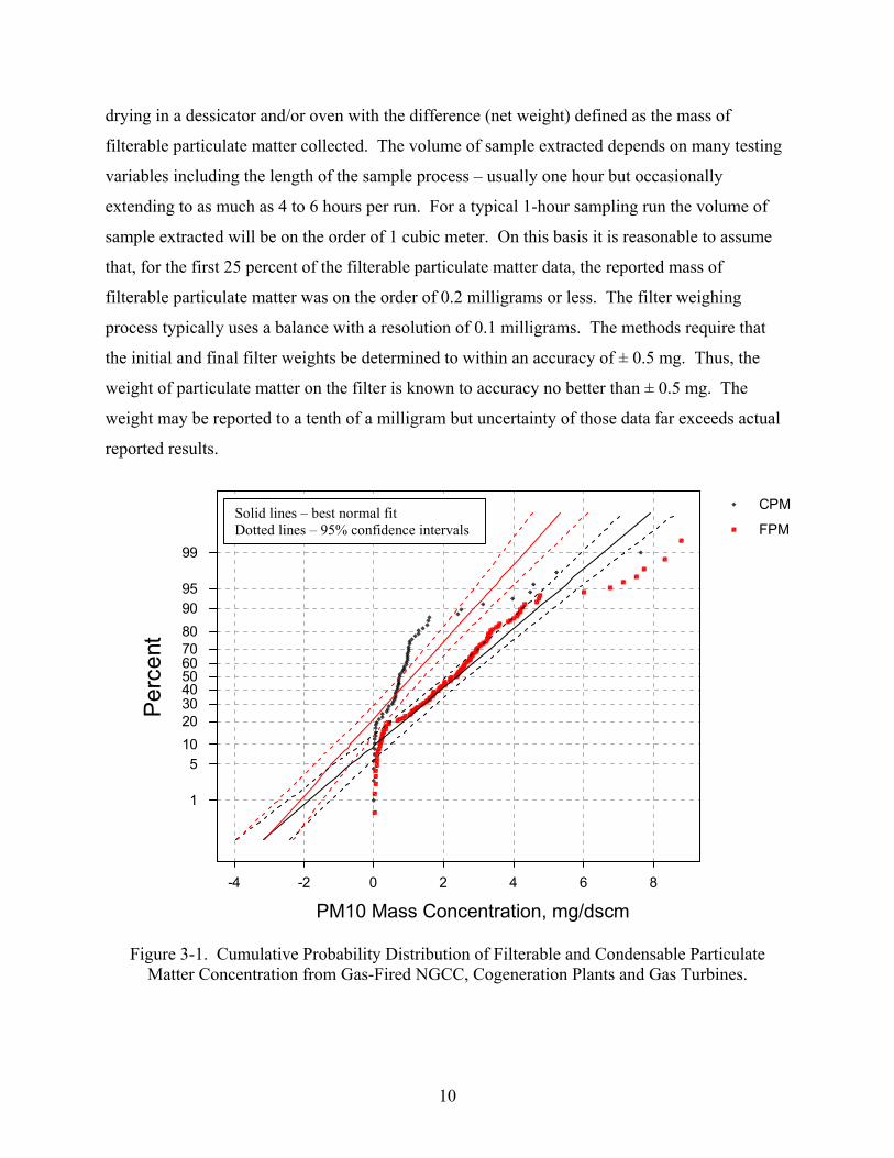
Examination of the data indicates extremely wide variation in both the filterable and condensable

PM mass concentrations from the various facilities. The concentration of filterable particulate

matter varied from essentially zero to nearly 9 mg/dscm. Similarly, the condensable particulate

matter concentrations ranged from essentially zero to about 7.5 mg/dscm. To further examine

trends, data were rank ordered and plotted on a normal cumulative probability plot (Figure 3-1).

Also included on the plot are results from regression analysis (solid lines) for the means and 95

percent confidence intervals (dotted lines) assuming that the data are normally distributed.

The filterable particulate matter data shows potentially explainable trends. As seen in the

probability plot, the first 25 percent of the data is from tests where filterable PM is reported to be

less than about 0.2 lb/hr and appear as an almost vertical line segment on the probability plot.

Next, there is a large segment of data covering 25 percent to 90 percent that are ordered in a very

linear fashion. Finally, there is a third group of filterable particulate matter data (the last 10

percent) that appear to follow a different slope on the probability curve.

The next section of this report addresses measurement methods in some detail but the more basic

concepts can be used here to place the filterable particulate matter data into context.

Measurement of filterable particulate matter involves extracting a sample of the flue gas and

passing that sample through a filter. The weight of the filter is determined pre-and post-test after

9

Data

Per

cent

99

95 90 80 70 60 50 40 30 20 10 5

1

Solid lines – best normal fit Dotted lines – 95% confidence intervals

-4 -2 0 2 4 6 8

CPM

FPM

PM10 Mass Concentration, mg/dscm

drying in a dessicator and/or oven with the difference (net weight) defined as the mass of

filterable particulate matter collected. The volume of sample extracted depends on many testing

variables including the length of the sample process – usually one hour but occasionally

extending to as much as 4 to 6 hours per run. For a typical 1-hour sampling run the volume of

sample extracted will be on the order of 1 cubic meter. On this basis it is reasonable to assume

that, for the first 25 percent of the filterable particulate matter data, the reported mass of

filterable particulate matter was on the order of 0.2 milligrams or less. The filter weighing

process typically uses a balance with a resolution of 0.1 milligrams. The methods require that

the initial and final filter weights be determined to within an accuracy of ± 0.5 mg. Thus, the

weight of particulate matter on the filter is known to accuracy no better than ± 0.5 mg. The

weight may be reported to a tenth of a milligram but uncertainty of those data far exceeds actual

reported results.

Figure 3-1. Cumulative Probability Distribution of Filterable and Condensable Particulate Matter Concentration from Gas-Fired NGCC, Cogeneration Plants and Gas Turbines.

10

A further consideration on the first section of the filterable particulate matter data involves a

classical problem associated with PM measurement. Following a test, the filter must be removed

from its holder for shipment back to the lab for analysis. It is not unusual for the filter to stick to

the holder during the sampling process and for small fibers of the filter to be torn away as the

filter is lifted from the holder. For sampling events with extremely low actual particulate

loadings, the weight of the torn fibers can equal or exceed the mass of collected particulate

matter. Assuming perfectly accurate gravimetric analysis in the laboratory, the measured

quantity of particulate matter collected can be negative. Since a negative mass makes no sense

physically, most firms count and report the negative mass as zero. Some firms may report the

negative filter mass, provided care is taken to recover any lost filter fragments in the other

sample fractions (e.g., in the acetone rinse of the front half of the filter housing and the filter

support), although this is not common.

Considering the accuracy limitations for gravimetric analysis and the existence of negative

weight gain, it is not surprising that the first portion of the probability plot does not conform to

the remainder of the data set. As noted earlier the vast majority of the filterable particulate

matter data (data representing 25 percent to 90 percent of the data) follows a classical normal

probability distribution. The final segment of the filterable particulate matter data set (the last 10

percent of the data) appears to have a different characteristic from the remainder of the data. For

this segment, it is likely that some key factor or factors were occurring which biases these data

from the remainder of the data set. Those factors might have to do with external conditions

during the test, a different type of fuel being burned, a problem with sampling process or a

problem in the laboratory. The range of potential factors will be discussed in the next section of

the report.

Condensable particulate measurements were made for some but not all of the tests shown in

Figure 3-1. There appears to be less variability in the total emissions than in the filterable

emissions, however this is somewhat misleading because of no all of the filterable particulate

measurements have corresponding condensable particulate results and in a small number of tests

in the middle range condensable particulate matter was reported together with filterable

particulate matter. There are no easy explanations for the trends. From a probability

perspective, there appear to be as many as five different segments to the curve. This may be due

11

to several factors affecting known artifacts (e.g., conversion of SO2 to solid residue in the

impingers, ammonia effects, etc.) that are neither well known nor controlled during the tests and

analysis. Clearly the data does not follow a normal distribution and is being significantly

influenced by factors other that random variation. Consideration of potential data drivers is

provided in the next section.

12

4. POTENTIAL SOURCES OF VARIABILITY IN GAS TURBINE PM EMISSIONS DATA

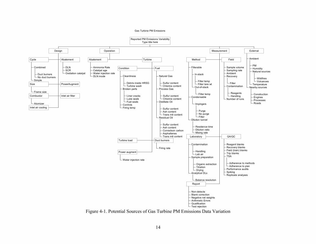
An internal meeting was held to brainstorm ideas on potential sources of the observed data

variability discussed in the previous chapter. The objective of this meeting was to capture as

many potential root causes as possible without regard to the likelihood of a specific potential

cause being a major contributor. To provide structure to the process, potential sources of data

variability were divided into three major categories:

• Process Design and Operation,

• Measurements, and

• External causes.

An overall summary of the brainstorming session is presented in Figure 4-1. The following

subsections discuss the results for each of the three areas.

PROCESS DESIGN AND OPERATION

There are a wide variety of gas turbine systems in operation today and it is certainly possible that

differences in the design, fuels, overall system configuration, operating mode, and installed

emissions control equipment could contribute to variation in the actual PM emissions.

Process Design

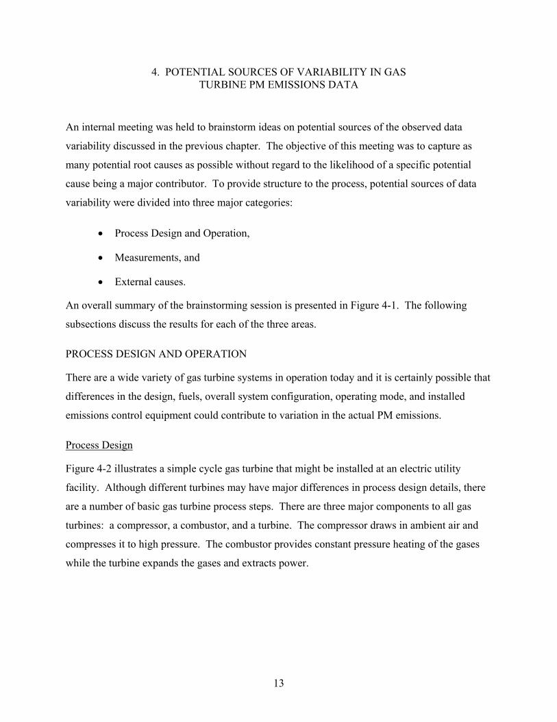
Figure 4-2 illustrates a simple cycle gas turbine that might be installed at an electric utility

facility. Although different turbines may have major differences in process design details, there

are a number of basic gas turbine process steps. There are three major components to all gas

turbines: a compressor, a combustor, and a turbine. The compressor draws in ambient air and

compresses it to high pressure. The combustor provides constant pressure heating of the gases

while the turbine expands the gases and extracts power.

13

Gas Turbine PM Emissions

Duct burners No duct burners

Combined

Simple

Cycle

DLN SCR Oxidation catalyst

Abatement

Frame size

Size PowerAugment

Atomizer

Combustor Inlet air filter

Inlet air cooling

Design

Ammonia Rate Catalyst age Water injection rate DLN mode

Abatement

Debris inside HRSG Turbine wash

Cleanliness

Liner cracks Lube seals Fuel seals

Broken parts

Controls Firing temp

Condition

Sulfur content Chlorine content

Natural Gas

Sulfur content Chlorine content

Process Gas

Sulfur content Ash content Trans mtl content

Distillate Oil

Sulfur content Ash content Conradson carbon Asphaltenes Trans mtl content

Residual Oil

Fuel

Turbine load

Firing rate

Duct burners

Power augment

Turbine

Operation

Filter temp Filter tare wt

In-stack

Filter temp

Out-of-stack

Filterable

Purge No purge Filter

Impingers

Condensable

Residence time Dilution ratio Mixing rate

Dilution tunnel

Method

Sample volume Sampling rate Ambient

Filter

Recovery

Reagents Handling

Contamination

Number of runs

Field

Measurement

PM Humidity

Wildfires Volcanoes

Natural sources

Temperature

Ambient

Construction Engines Processes Roads

Nearby sources

External

Reported PM Emissions Variability Type title here

Water injection rate

Handling Lab air

Contamination

Organic extraction Titration Drying

Sample preparation

Balance resolution

Analytical DLs

Laboratory

Reagent blanks Recovery blanks Field (train) blanks Trip blanks

Adherence to methods Adherence to plan

TSA

Performance audits Spiking Replicate analyses

QA/QC

Report

Non-detects Blank correction Negative net weights Arithmetic Errors Qualification Test rejection

Figure 4-1. Potential Sources of Gas Turbine PM Emissions Data Variation

14

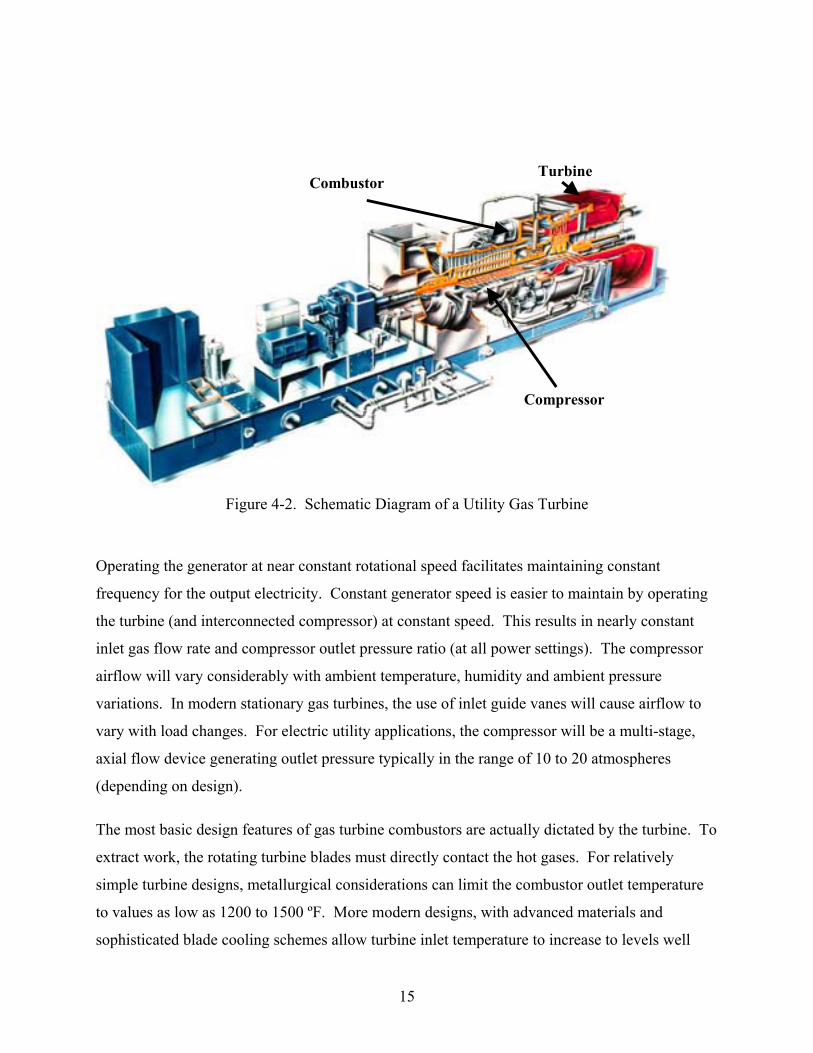
Turbine

Compressor

Combustor

Figure 4-2. Schematic Diagram of a Utility Gas Turbine

Operating the generator at near constant rotational speed facilitates maintaining constant

frequency for the output electricity. Constant generator speed is easier to maintain by operating

the turbine (and interconnected compressor) at constant speed. This results in nearly constant

inlet gas flow rate and compressor outlet pressure ratio (at all power settings). The compressor

airflow will vary considerably with ambient temperature, humidity and ambient pressure

variations. In modern stationary gas turbines, the use of inlet guide vanes will cause airflow to

vary with load changes. For electric utility applications, the compressor will be a multi-stage,

axial flow device generating outlet pressure typically in the range of 10 to 20 atmospheres

(depending on design).

The most basic design features of gas turbine combustors are actually dictated by the turbine. To

extract work, the rotating turbine blades must directly contact the hot gases. For relatively

simple turbine designs, metallurgical considerations can limit the combustor outlet temperature

to values as low as 1200 to 1500 ºF. More modern designs, with advanced materials and

sophisticated blade cooling schemes allow turbine inlet temperature to increase to levels well

15

above 2000 ºF, typically on the order of 2500 ºF in the current generation of large stationary gas

turbines and up to 2600 ºF in the latest, state-of-the-art high efficiency stationary gas turbine

designs. This temperature limitation applies to all turbine power levels. Since the maximum

temperature occurs at maximum power setting, reduced power or idle conditions will necessarily

have much lower turbine inlet temperature.

There are several combustor design implications to the turbine inlet temperature limitations. A

natural gas flame with a near stoichiometric fuel-to-air ratio will produce a peak temperature of

nearly 3500 ºF – well above the upper inlet temperature limit for even the most modern

commercial turbines. To control the combustor exit temperature, combustors are operated at

high overall excess air levels. The full load operating condition will vary between designs but a

typical turbine will have about 12 to 15 percent oxygen in its exhaust at maximum power,

depending on the size and vintage of the unit. This is achieved by supplying air at about 3 times

the stoichiometric requirement. For reduced power settings, even higher excess air levels are

required. Inlet guide vanes installed on many units reduce the inlet airflow as load to maintain

higher turbine inlet temperatures and hence higher efficiency at reduced power settings.

The flame in the combustor must be stable over the entire operating envelope. Unless the fuel

and air mixing process is carefully controlled, attempting to burn fuel with high levels of excess

air can result in unstable operation. To maintain flame stability, gas turbine combustors are

designed to mix only a portion of the total system flow with the fuel at the beginning of the

combustion process. The remainder of the air is sequentially added down the length of the

combustor. This allows the combustion air to provide cooling for the combustor walls while

maintaining a stable combustion process. The final portion of air addition serves primarily as a

dilution process, to achieve the desired overall mean combustor exit temperature level and to

tailor the temperature profile of the gases entering the turbine.

When the hot, high-pressure gases from the combustor enter the turbine, power is extracted by

expansion. The pressure level drops from levels commensurate with the compressor exit to near

ambient conditions. The gas temperature also drops. The turbine exit temperature will vary

depending on the power setting or turbine inlet temperature. For a modern, large frame machine

the turbine exit temperature will be on the order of 1000 to 1200 ºF at maximum power. These

16

exhaust gases contain a relatively high level of sensible heat. To enhance the overall cycle

efficiency, many electric utility gas turbines are equipped with exhaust gas heat recovery

components. Such systems are essentially boilers or heat exchangers that cool the gases while

generating steam. The major components may be as simple as a steam/air heat exchanger or the

unit may burn additional fuel to generate larger quantities of steam. The produced steam can

then be used to turn a steam turbine powering a separate electrical power generator.

Within the context of providing the above basic system components, there are many design and

configuartional differences among different gas turbines. The major process design features

identifies as potentially impacting gas turbine PM emissions included:

• Unit Size.

• Operating Cycle

• Power Augmentation

• Combustor Design Type

• Post-combustion air pollution control equipment installed

Unit Size. Gas turbines are manufactured and installed in a wide size range. Units are installed

with ratings as small as few hundred kilowatts for emergency power generation while large

combined cycle gas turbines for utility application can produce nearly 300 MW. Power output

from a gas turbine is directly proportional to the mass flow rate of gases passing through the

turbine. Holding other factors constant, variations of gas flow rate between different turbines

should have little direct impact on a turbine’s PM emission quantity or the speciation of trace

constituents that contribute to the condensable portion of the PM emissions. One possible

impact of changing mass flow of gases processed by the turbine is the potential for change in the

quantity of debris drawn in by the turbine. However, as long as the facility’s inlet system is

appropriately adjusted to account for the increased airflow rate, the relative concentration of

injected debris should be relatively constant.

A second impact of unit size is that the total quantity of fuel burned in the turbine increases with

power output. Thus, the mass emission rate of particulate matter directly associated with a fuel

17

constituent (such as the ash content of a liquid fuel) should be expected to increase with

increasing unit size. If the overall power generating efficiency (heat rate) of different turbine

sizes is approximately constant, the concentration of particulate matter should also remain

roughly constant even though the mass emission rate increases. Finally, there is a general trend

toward larger gas turbine systems having higher overall efficiency. Accordingly, large turbines

with high efficiency might potentially have lower particulate matter exhaust concentration than

small units with lower efficiency.

Operating Cycle. The above discussion of unit size, noted that the efficiency of an installation

might have a direct effect on PM emissions since the relative quantity of fuel consumed

decreases with increasing efficiency. Significant increases in overall efficiency can be realized

by changing a turbine from a simple cycle design to a combine cycle design. Moreover, the heat

recovery equipment may be either an air-to-water heat exchanger or the system may be equipped

with a duct burner to further increase the quantity of power generated in the steam cycle. To the

extent that the relative quantity of fuel consumed might directly impact gas turbine PM

emissions, such a trend might be discernable through examination of emissions results for similar

size facilities but with different operating cycle.

It is also possible that there could be an impact of the facility’s power cycle on the quantity of

condensable particulate matter released. Such an impact might occur through complex chemical

processes such as an impact on the concentration of nitrates and sulfates in the stack. At

temperatures commensurate with levels that occur in gas turbine combustors and turbine sections

(at full load), species such as NOx and SOx are almost exclusively in the form of NO and SO2.

As temperature drop toward ambient conditions, there is a shift in thermodynamic equilibrium

toward NO2 and SO3. However, chemical kinetic barriers only allow that conversion to occur at

a slow rate (relative to the residence time of the gases in the turbine or the heat recovery steam

generator (HRSG). The oxidation reactions can occur rapidly in the presence of certain catalysts.

Stainless steel is one of the classic catalysts for oxidizing NO to NO2. Thus it is possible that

passing the turbine exhausts through a HRSG might impact the relative quantity of NO2 or SO3

in the facility exhaust. This could, in turn impact the quantity of condensable particulate matter

released. Though possible, this potentiality must be considered remote. Available NOx

18

emissions data do not indicate a significant trend of higher NO2 emissions from combined cycle

turbines than from simple cycle systems.

Inlet Air Filtration. Many large turbine facilities are equipped with filters in the inlet air system

to limit the quantity of entrained debris entering the turbine. These devices are installed

primarily to protect the turbine internal parts from erosion and corrosion. Presence or absence of

an inlet air filter could also impact the quantity of filterable particulate mater in the stack.

Accordingly, it is possible that presence of an air filter as well as the maintenance state of that

filter could impact the variability of turbine exhaust PM emissions data. Filters could be

particularly important in preventing large diameter particle ingestion.

Power Augmentation. A number of approaches can be used to augment the overall power output

from a turbine installation. One approach is to inject water into the process either at a mid point

in the compressor or into the combustor. The added water increases mass flow through the

turbine, which increases power output. A second approach is to add an inner cooler at a mid

point in the compressor. The use of inner cooling will increase the efficiency of a gas turbine but

should have little impact on PM emissions outside those considerations discussed above for unit

size and efficiency. Use of water injection may have an additional impact since the mineral and

organic impurities in the water may increase the level of filterable particulate matter.

Combustor Design. General issues associated with gas turbine combustor design, including

excess air levels, flame stability, and turbine inlet temperature were discussed earlier. Prior to

the advent of NOx emissions requirements, gas turbine combustors were typically designed to

provide near stoichiometric fuel/air ratio at the dome section of the combustor and then to

sequentially add additional air through slots in the combustor wall. The initial fuel/air mixing

process was designed to occur as rapidly as possible, typically with a diffusion flame. This

configuration provided maximum flame stability and allowed for very compact combustor

hardware. Unfortunately, that general design also tended to provide relatively high NOx

emissions. The advent of environmental regulations (beginning in the mid 1970s) drove major

advances in gas turbine combustor design.

Since gas turbines are generally fired with fuels such as natural gas or distillate oil that contain

essentially no chemically bound nitrogen, the primary route for NOx formation is oxidation of

19

molecular nitrogen in air. The controlling chemistry for this process is relative well understood

and is driven by local temperature in the burning process. In fact, for any give pressure and fuel

air ratio, the rate of NOx formation increases exponentially with local temperature. Two basic

approaches were used to limit local peak flame temperature and to control NOx formation. The

first approach was to inject water into the head end of the combustor. Vaporization of the water

consumed a portion of the heat release and resulted in a decrease in local, peak flame

temperature. This is an effective approach that is still widely applied for stationary turbines

firing oil. There are certainly adverse impacts of water injection but there is at least one positive

side benefit. Since power output is directly proportional to the mass flow of gases passing

through the turbine, water addition generates a small positive increment in power generation.

The second basic combustor design approach used controlling peak flame temperature (and NOx

emissions) is to premix (or rapidly mix) the inlet fuel and air and to increase the stoichiometric

ratio of gases in the inlet region (more fuel lean). If a combustor generates a classical diffusion

flame, there will be a fuel-rich core and an air-rich outer zone with the flame front itself located

at the interface where the mixture is at near stoichiometric conditions. That condition provides

maximum local temperature and maximum local NOx production. If the fuel and air can be

premixed, the local flame temperature will be consistent with the local stoichiometry. By going

to more fuel-lean mixtures, it is possible to suppress the local peak temperature and to achieve a

commensurate decrease in NOx production. The critical issue is accomplishing this change while

maintaining combustion stability over the complete envelope of system operation – including

full- power, low-load, idle, and start-up as well as transitioning between the various power

conditions.

As discussed above, gas turbine combustors may be of the conventional design, may be with or

without water injection, or may be of the more modern design broadly referred to as dry low NOx

combustion. These variations in combustor design may have a slight impact on the measured

level of condensable particulate matter and thus may impact the observed variability in PM

emissions data. One of the clear potential impacts is through the variation in NO2 emissions – a

water-soluble species that may react to form a nitrate that would contribute to the condensable

fraction of PM. Note that NO is the predominant constituent in NOx from turbines and variations

in NO should not impact PM emissions. However, since NO2 is typically formed in the lower

20

temperature regions, including in the HSRG, variations in total NOx could indirectly contribute

to variations in condensable PM emissions. A second avenue for potential PM impact is through

variation in the level of carbonaceous particulate matter produced. Gas turbines generally

achieve high combustion efficiency levels and create only trace levels of unburned carbon or

higher organic compounds that might contribute to condensable PM. However, the total PM

loading from gas turbines is extremely small and variations in carbonaceous particulate matter

could contribute to the observed variability in PM emissions.

Post-combustion air pollution control equipment. Many gas turbines comply with federal, state,

and local air pollution requirements without use of add on air pollution control equipment.

However, in key areas such as California, more stringent state and local regulations have led to

broad application of selective catalytic reduction (SCR) for enhanced NOx control. Some units

are also being equipped with oxidation catalysts. Presence of these add-on devices could have an

impact on the level of both filterable and condensable particulate matter. Filterable particulate

matter could be impacted through processes such as erosion of the catalysts material in either an

SCR or an oxidation catalyst.

For an SCR there are at least two avenues by which PM emissions could be impacted. SCRs

destroy NOx through reactions with ammonia (or urea) forming molecular nitrogen and water as

by products. Reagent suppliers blend anhydrous ammonia with either distilled/deionized (DI)

water or with water processed through a reverse osmosis (RO) process. Typically, aqueous

ammonia is procured with about 20 to 30 percent ammonia in the water. Any impurities in the

water used to generate the reagent (usually calcium based compounds) will eventually

contribute to the level of filterable particulate matter in the turbine exhaust. An additional

contribution to PM could come from ammonia that slips through the SCR. In a typical SCR

application, ammonia slip concentration will be on the order of 1 to 10 ppm. Ammonia is highly

soluble in water and thus will be captured in the condensable portion of most PM sampling

systems. Free NH3 in the samples can increase the amount of dissolved SO2, and thereby

increase artifact sulfate formation, since it instantly reacts in aqueous solution forming

ammonium sulfite/bisulfite ions and additional SO2 must dissolve to maintain equilibrium

(Seinfeld and Pandis, 2000).

21

For an oxidation catalyst, at least two potential processes can lead to variability in PM emissions

results. First the catalyst is provided to reduce the level of CO and other organics emitted from

the turbine. Presence of an oxidation catalyst could clearly result in reduced levels of

carbonaceous material in a facility’s stack. The oxidation step is not limited to organics,

however. These catalysts can also be effective at oxidizing NO to NO2. The potential impact of

increased NO2 on condensable PM emissions was discussed above.

Overall, the presences of add on air pollution control devices to the exhaust of a gas turbine

installation could certainly impact PM emissions and/or the measurement of PM emissions,

positively or negatively. Moreover, variation in the design and operation of those add-on devices

could have a variable impact on PM emissions and contribute to the variability seen in the

existing database.

Process Operation

The previous section discussed how basic system configuration could potentially impact PM

emissions from gas turbine installations. This section discusses how system operations could

impact PM emissions.

There are several key parameters in the turbine, HRSG, and emission abatement system

operation that could influence PM emissions. These key parameters can be grouped into the

following categories:

• Fuels,

• Equipment Condition, and

• Operating Rate.

Additionally there are key operating parameters associated with the emission abatement systems

included at a facility.

Fuels. Turbines and fired HSRGs may burn any of a variety of fuels including natural gas,

process gas, distillate oil and some units can be operated on residual fuel oil. Table 4-1

summarizes the key characteristics for each fuel type that might have an impact on a turbine’s

22

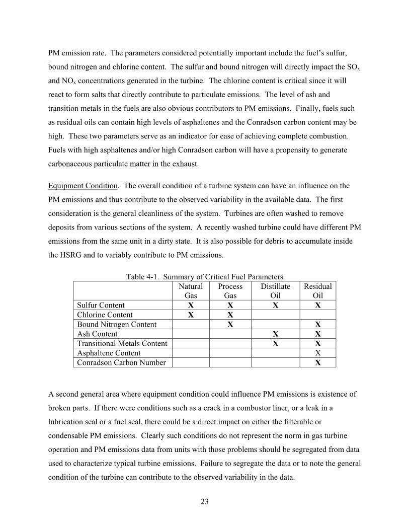
PM emission rate. The parameters considered potentially important include the fuel’s sulfur,

bound nitrogen and chlorine content. The sulfur and bound nitrogen will directly impact the SOx

and NOx concentrations generated in the turbine. The chlorine content is critical since it will

react to form salts that directly contribute to particulate emissions. The level of ash and

transition metals in the fuels are also obvious contributors to PM emissions. Finally, fuels such

as residual oils can contain high levels of asphaltenes and the Conradson carbon content may be

high. These two parameters serve as an indicator for ease of achieving complete combustion.

Fuels with high asphaltenes and/or high Conradson carbon will have a propensity to generate

carbonaceous particulate matter in the exhaust.

Equipment Condition. The overall condition of a turbine system can have an influence on the

PM emissions and thus contribute to the observed variability in the available data. The first

consideration is the general cleanliness of the system. Turbines are often washed to remove

deposits from various sections of the system. A recently washed turbine could have different PM

emissions from the same unit in a dirty state. It is also possible for debris to accumulate inside

the HSRG and to variably contribute to PM emissions.

Table 4-1. Summary of Critical Fuel Parameters Natural

Gas Process

Gas Distillate

Oil Residual

Oil Sulfur Content X X X X Chlorine Content X X Bound Nitrogen Content X X Ash Content X X Transitional Metals Content X X Asphaltene Content X Conradson Carbon Number X

A second general area where equipment condition could influence PM emissions is existence of

broken parts. If there were conditions such as a crack in a combustor liner, or a leak in a

lubrication seal or a fuel seal, there could be a direct impact on either the filterable or

condensable PM emissions. Clearly such conditions do not represent the norm in gas turbine

operation and PM emissions data from units with those problems should be segregated from data

used to characterize typical turbine emissions. Failure to segregate the data or to note the general

condition of the turbine can contribute to the observed variability in the data.

23

Finally, the general condition of the emission abatement system can be an important variable in

determining the PM emissions from a turbine installation. As noted previously, erosion of

catalysts can directly contribute to filterable PM emissions.

Operating Rates. The previous discussion on gas turbine design noted several areas where

operating rates could directly impact PM emissions. These include the turbine load, the firing

rate of the duct burner (if present) and the rate of water injection for power augmentation or for

NOx abatement. Clearly, variations in any of these parameters could have a direct or indirect

impact on PM emissions.

An additional operating parameter of importance is the ammonia injection rate to the SCR

system. Many SCR control systems adjust the ammonia injection rate to achieve a desired NOx

emission rate. As the catalyst ages or becomes poisoned, achieving the set point requires

increasing the ammonia injection rate. This can directly impact the ammonia slip level, which

can have a direct impact on the measured level of condensable emissions.

MEASUREMENTS

The previous portion of this chapter addressed how the design and operation of a gas turbine

installation might impact the PM emissions from the facility. Variations in those parameters

might contribute to variability in the actual PM emissions. An equally important consideration is

the system used to measure PM emissions. There are many different methods used to make PM

measurements and various factors can influence the precision and accuracy of the results. This

portion of the report briefly describes the various test procedures being used and then examines

various factors that could impact the results achieved through their use.

Measurement Methods

The Introduction section of this report provided broad background information of methods used

to measure PM emissions from turbines. There are four basic types of systems used to make the

measurements, including:

• In-stack filter methods,

• Out-of-stack filter methods,

24

• Impinger methods, and

• Dilution methods.

Each of the basic approaches is discussed in the following sections. It should be noted, however,

that the vast majority of the data on gas turbine PM emissions has been gathered using impinger

methods.

In-Stack Filter Methods. The primary example of an in-stack filter method is the US EPA’s

Method 17. Use of this method is strictly limited to measurement of filterable particulate matter

and is normally applied to stack containing gases that may condense at temperature below the

stack temperature but above 250 ºF. In this method a pre-weighed filter is inserted into the stack

and sample is pulled through the filter at a rate to achieve isokinetic conditions. External to the

stack a series of iced impingers is provided to cool the sample and to dry the gases to a dew point

near 32 ºF. Following the impingers are a dry gas meter and a sample pump. The dry gas meter

is used to determine the volume of dry sample extracted. The location of the sampling probe and

in-stack filter is moved to different positions in the stack to obtain a spatially representative

sample. At the end of the sampling period, the probe is removed and weight gain of the filter

determined. The ratio of the filter weight gain and the measured sample volume are used to

calculate the concentration of filterable particulate matter in the stack.

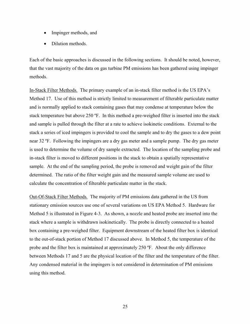
Out-Of-Stack Filter Methods. The majority of PM emissions data gathered in the US from

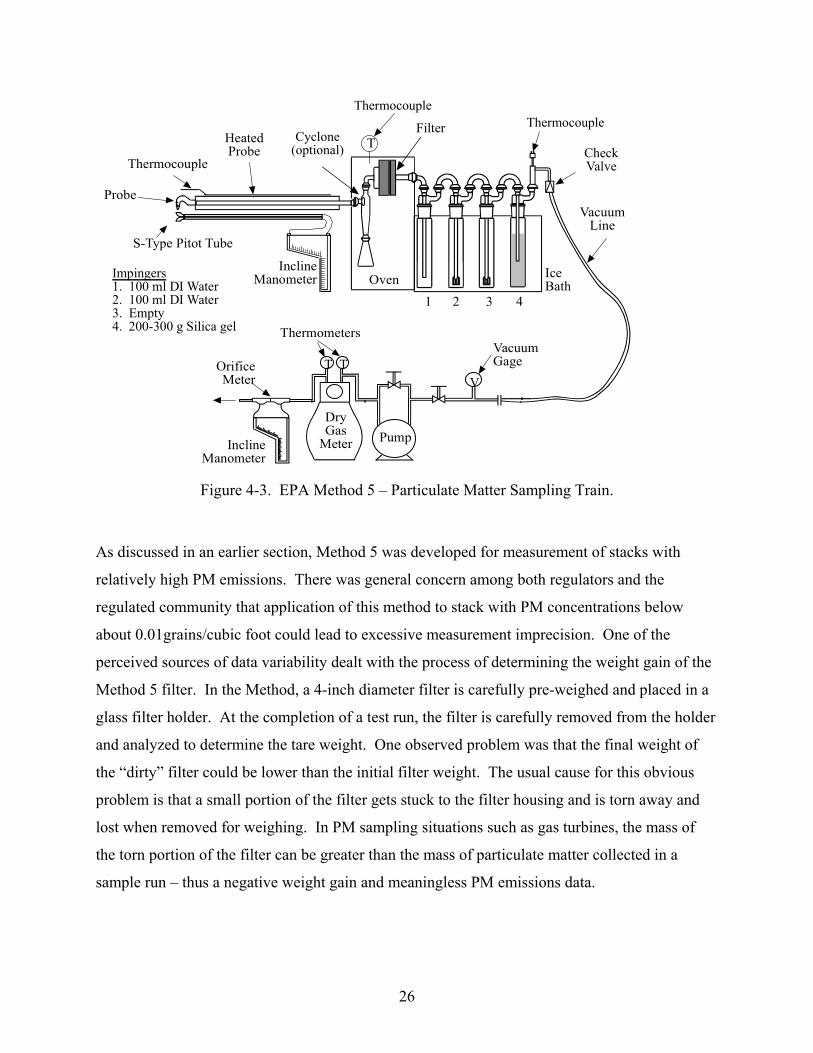
stationary emission sources use one of several variations on US EPA Method 5. Hardware for

Method 5 is illustrated in Figure 4-3. As shown, a nozzle and heated probe are inserted into the

stack where a sample is withdrawn isokinetically. The probe is directly connected to a heated

box containing a pre-weighed filter. Equipment downstream of the heated filter box is identical

to the out-of-stack portion of Method 17 discussed above. In Method 5, the temperature of the

probe and the filter box is maintained at approximately 250 ºF. About the only difference

between Methods 17 and 5 are the physical location of the filter and the temperature of the filter.

Any condensed material in the impingers is not considered in determination of PM emissions

using this method.

25

Thermocouple

Thermocouple

Heated Probe

Cyclone(optional) T

Filter Thermocouple

Check Valve

Probe

S-Type Pitot Tube

Vacuum Line

Impingers1. 100 ml DI Water

Incline Manometer Oven Ice

Bath 2. 100 ml DI Water 1 2 3 4 3. Empty4. 200-300 g Silica gel Thermometers

Vacuum Orifice T T Gage Meter V

DryGas Pump Meter

Manometer Incline

Figure 4-3. EPA Method 5 – Particulate Matter Sampling Train.

As discussed in an earlier section, Method 5 was developed for measurement of stacks with

relatively high PM emissions. There was general concern among both regulators and the

regulated community that application of this method to stack with PM concentrations below

about 0.01grains/cubic foot could lead to excessive measurement imprecision. One of the

perceived sources of data variability dealt with the process of determining the weight gain of the

Method 5 filter. In the Method, a 4-inch diameter filter is carefully pre-weighed and placed in a

glass filter holder. At the completion of a test run, the filter is carefully removed from the holder

and analyzed to determine the tare weight. One observed problem was that the final weight of

the “dirty” filter could be lower than the initial filter weight. The usual cause for this obvious

problem is that a small portion of the filter gets stuck to the filter housing and is torn away and

lost when removed for weighing. In PM sampling situations such as gas turbines, the mass of

the torn portion of the filter can be greater than the mass of particulate matter collected in a

sample run – thus a negative weight gain and meaningless PM emissions data.

26

To circumvent the filter problem, the US EPA adapted a procedure pioneered in Europe and

developed Method 5i. In Method 5i, the filter and filter holder hardware are different than in

Method 5. A 52 mm diameter filter, frit, and filter holder are assembled as a composite unit and

pre-weighed. At the completion of a test, the composite assembly is recovered and weighed.

This eliminates the possibility of tearing off a portion of the filter during the recovery process.

The drawback to this method is that the combined mass of the filter, frit, and holder assembly is

high relative to the mass of particulate matter collected. Thus, the net sample weight is a small

difference between two large numbers (the weights of the assembly before and after the test) – a

classic contributor to measurement imprecision.

Impinger Methods. Several methods have been developed that attempt to determine the emission

rate of condensable material. These methods are generally an adaptation of procedures such as

Method 5 but providing for analysis of the material collected in the impingers downstream of the

filter. In its simplest form, some states require that the impinger water plus condensed sample

gas constituents be analyzed for condensed phase material and those results reported as

condensable particulate matter. It is common convention to refer this as an EPA 5 “back half”

procedure.

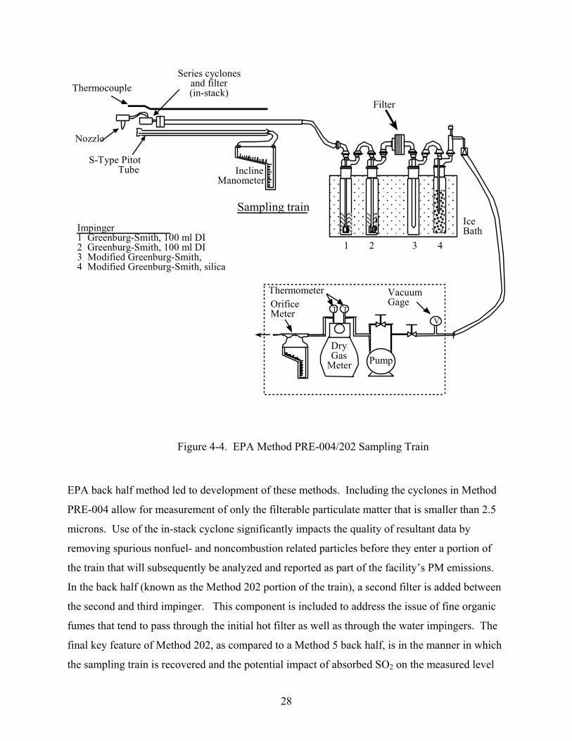
To standardize the analytical procedures used for the back half analysis, EPA published Method

202. This procedure has been further refined into a procedure now designated as PRE-004 as

illustrated in Figure 4-4. As shown, the hardware incorporates an in-stack 10µm and a 2.5µm

cyclone upstream of an in-stack filter. This as followed by an iced impinger train using water as

the impinger solution. Method 202 uses the same hardware except that it does not include the

cyclone separators. Two known problems with the

27

Series cyclonesand filter

Impinger1 Greenburg-Smith, 100 ml DI2 Greenburg-Smith, 100 ml DI3 Modified Greenburg-Smith,4 Modified Greenburg-Smith, silica

Ice Bath

1 2 3 4

Filter

Thermometer

Pump

Vacuum Gage

DryGas

Meter

Orifice Meter

V TT

Sampling train

Thermocouple

S-Type PitotTube

Nozzle

(in-stack)

Incline Manometer

Figure 4-4. EPA Method PRE-004/202 Sampling Train

EPA back half method led to development of these methods. Including the cyclones in Method

PRE-004 allow for measurement of only the filterable particulate matter that is smaller than 2.5

microns. Use of the in-stack cyclone significantly impacts the quality of resultant data by

removing spurious nonfuel- and noncombustion related particles before they enter a portion of

the train that will subsequently be analyzed and reported as part of the facility’s PM emissions.

In the back half (known as the Method 202 portion of the train), a second filter is added between

the second and third impinger. This component is included to address the issue of fine organic

fumes that tend to pass through the initial hot filter as well as through the water impingers. The

final key feature of Method 202, as compared to a Method 5 back half, is in the manner in which

the sampling train is recovered and the potential impact of absorbed SO2 on the measured level

28

of sulfates in the condensable fraction. Specifically, Method 202 requires that if the pH of the

impinger catch is les that 4.5, the impinger train should be post-test purged with nitrogen. This

procedure is an attempt to drive the absorbed SO2 from the impingers before it has an

opportunity to oxidize SO2 to SO3 and form sulfate.

There are many variations on the above-described EPA Method 202. Some of the major variants

concern initial filtration of the sample. The form of EPA Method 202 illustrated in Figure 4-4

included cyclones to separate particles larger than 2.5 microns from the remainder of the train. A

sampling system can be configured with only a 10µm cyclone or with no cyclone at all. Finally,

there are measurement methods such as EPA Modified EPA Method 8 that are specifically

designed to capture key constituents of PM such as the sulfate fraction. This method is

illustrated in Figure 4-5. The key differences between Modified Method 8 and Method 202 are

the impinger arrangement, the absorbents used in the impingers, and the analytical procedures

used to analyze the material collected in the impingers. Another example variation on Method

202 is South Coast Air Quality Management District Method 5.2 (SCAQMD, 2002[GCE1]), which

includes a different analytical finish on the impinger solutions to determine total acid and total

sulfates in addition to gravimetric analysis for mass. A subtraction allowed for the difference

between total acid and total sulfates, which is presumed to be sulfuric acid potentially, formed as

an artifact of gaseous SO2 oxidation to H2SO4 in the impingers during sampling/storage, and for

ammonia if present. EPA recently identified at least 7 significant variations in impinger methods

among 22 states surveyed (Riley and Myers, 2002). These variations can have significant impact

on the measured result, and are seldom taken into account in emission databases.

29

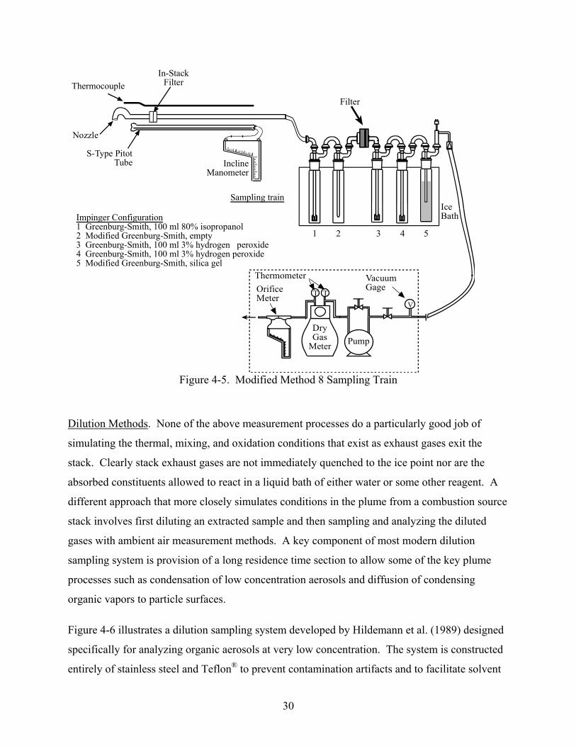
Thermocouple In-Stack

Filter

Filter

Nozzle

S-Type PitotTube Incline

Manometer

Impinger Configuration1 Greenburg-Smith, 100 ml 80% isopropanol2 Modified Greenburg-Smith, empty3 Greenburg-Smith, 100 ml 3% hydrogen peroxide4 Greenburg-Smith, 100 ml 3% hydrogen peroxide5 Modified Greenburg-Smith, silica gel

Sampling train

1 2 3 4 5

Ice Bath

Thermometer Vacuum Orifice Meter TT

Gage

V

DryGas

Meter Pump

Figure 4-5. Modified Method 8 Sampling Train

Dilution Methods. None of the above measurement processes do a particularly good job of

simulating the thermal, mixing, and oxidation conditions that exist as exhaust gases exit the

stack. Clearly stack exhaust gases are not immediately quenched to the ice point nor are the

absorbed constituents allowed to react in a liquid bath of either water or some other reagent. A

different approach that more closely simulates conditions in the plume from a combustion source

stack involves first diluting an extracted sample and then sampling and analyzing the diluted

gases with ambient air measurement methods. A key component of most modern dilution

sampling system is provision of a long residence time section to allow some of the key plume

processes such as condensation of low concentration aerosols and diffusion of condensing

organic vapors to particle surfaces.

Figure 4-6 illustrates a dilution sampling system developed by Hildemann et al. (1989) designed

specifically for analyzing organic aerosols at very low concentration. The system is constructed

entirely of stainless steel and Teflon® to prevent contamination artifacts and to facilitate solvent

30

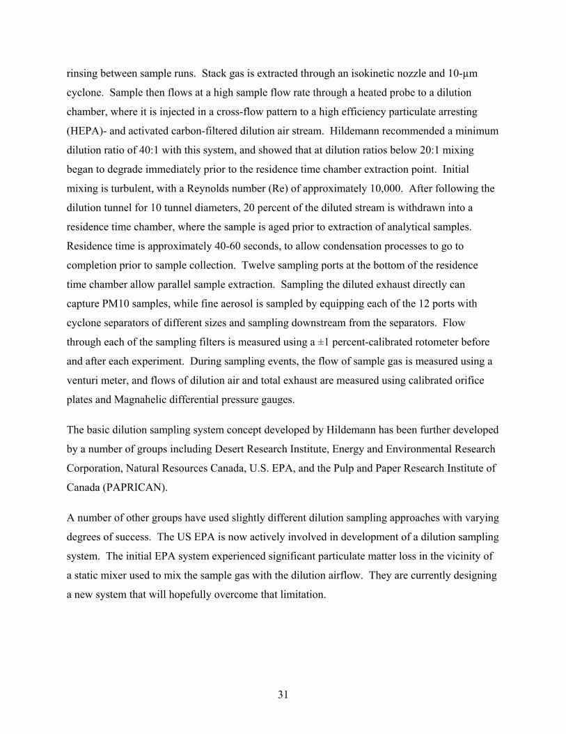
rinsing between sample runs. Stack gas is extracted through an isokinetic nozzle and 10-µm

cyclone. Sample then flows at a high sample flow rate through a heated probe to a dilution

chamber, where it is injected in a cross-flow pattern to a high efficiency particulate arresting

(HEPA)- and activated carbon-filtered dilution air stream. Hildemann recommended a minimum

dilution ratio of 40:1 with this system, and showed that at dilution ratios below 20:1 mixing

began to degrade immediately prior to the residence time chamber extraction point. Initial

mixing is turbulent, with a Reynolds number (Re) of approximately 10,000. After following the

dilution tunnel for 10 tunnel diameters, 20 percent of the diluted stream is withdrawn into a

residence time chamber, where the sample is aged prior to extraction of analytical samples.

Residence time is approximately 40-60 seconds, to allow condensation processes to go to

completion prior to sample collection. Twelve sampling ports at the bottom of the residence

time chamber allow parallel sample extraction. Sampling the diluted exhaust directly can

capture PM10 samples, while fine aerosol is sampled by equipping each of the 12 ports with

cyclone separators of different sizes and sampling downstream from the separators. Flow

through each of the sampling filters is measured using a ±1 percent-calibrated rotometer before

and after each experiment. During sampling events, the flow of sample gas is measured using a

venturi meter, and flows of dilution air and total exhaust are measured using calibrated orifice

plates and Magnahelic differential pressure gauges.

The basic dilution sampling system concept developed by Hildemann has been further developed

by a number of groups including Desert Research Institute, Energy and Environmental Research

Corporation, Natural Resources Canada, U.S. EPA, and the Pulp and Paper Research Institute of

Canada (PAPRICAN).

A number of other groups have used slightly different dilution sampling approaches with varying

degrees of success. The US EPA is now actively involved in development of a dilution sampling

system. The initial EPA system experienced significant particulate matter loss in the vicinity of

a static mixer used to mix the sample gas with the dilution airflow. They are currently designing

a new system that will hopefully overcome that limitation.

31

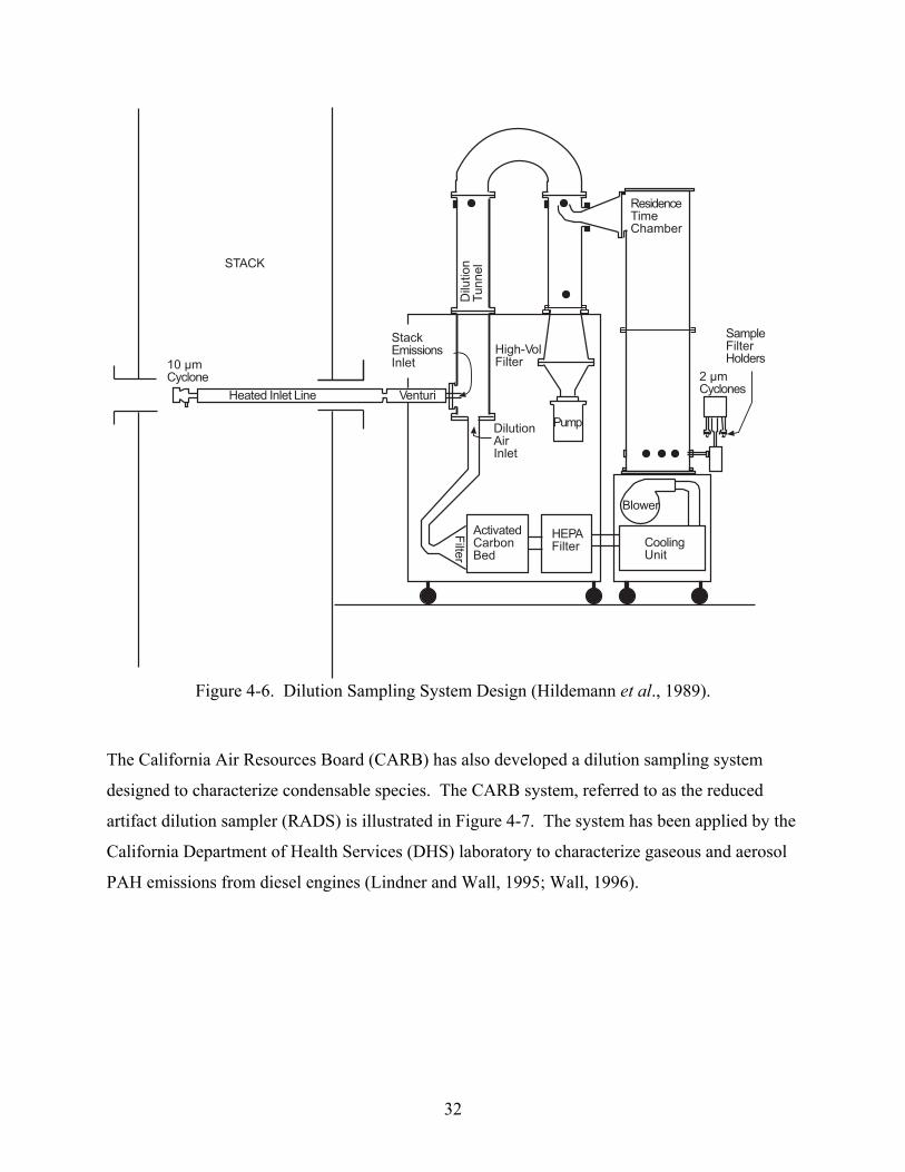
STACK

10 !m Cyclone

Heated Inlet Line

Stack Emissions Inlet

ent:ri

0il:tion Air Inlet

P:mp

0il:tion

T:nnel

Hi h ol Filter

Sample Filter Holders

2 !m Cyclones

Residence Time Chamber

Acti ated Carbon ed

HEPA Filter

Filter

lo er

Coolin �nit

Figure 4-6. Dilution Sampling System Design (Hildemann et al., 1989).

The California Air Resources Board (CARB) has also developed a dilution sampling system

designed to characterize condensable species. The CARB system, referred to as the reduced

artifact dilution sampler (RADS) is illustrated in Figure 4-7. The system has been applied by the

California Department of Health Services (DHS) laboratory to characterize gaseous and aerosol

PAH emissions from diesel engines (Lindner and Wall, 1995; Wall, 1996).

32

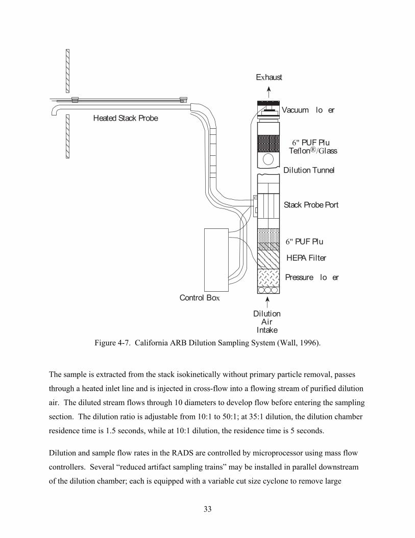
Exha:st

Control ox

Heated Stack Probe ac::m lo er

6" P� F Pl: Teflon®/Glass

0il:tion T:nnel

Stack Probe Port

6" P� F Pl:

HEPA Filter

Press:re lo er

0il:tion Air Intake

Figure 4-7. California ARB Dilution Sampling System (Wall, 1996).

The sample is extracted from the stack isokinetically without primary particle removal, passes

through a heated inlet line and is injected in cross-flow into a flowing stream of purified dilution

air. The diluted stream flows through 10 diameters to develop flow before entering the sampling

section. The dilution ratio is adjustable from 10:1 to 50:1; at 35:1 dilution, the dilution chamber

residence time is 1.5 seconds, while at 10:1 dilution, the residence time is 5 seconds.

Dilution and sample flow rates in the RADS are controlled by microprocessor using mass flow

controllers. Several “reduced artifact sampling trains” may be installed in parallel downstream

of the dilution chamber; each is equipped with a variable cut size cyclone to remove large

33

particles upstream of the sample media, followed by a denuder, a 5-inch Teflon® filter to capture

particulate matter, and a 6-inch diameter PUF cartridge for absorption of gaseous PAH.

Sample Collection (Field Procedures)

The preceding section described the basic methods used to collect PM emissions data from a

wide variety of source types. The majority of the available data from gas turbines has been

developed using methods similar to that described as EPA Method PRE-004 involving cyclone

filters to remove any large diameter particles, a heated filter to catch particles followed by a

series of iced impingers to collect condensable particulate matter. The current section discusses

how this type of sampling system is applied in the field along with discussion of various ways

that the field procedures may influence data variability.

The formal EPA measurement method recognize that the concentration of pollutants may not be

constant across a stack, that sources do not always operate in exactly the same manner over an

extended time period, and that there can be data variability introduced by the field testing

technicians. Accordingly, the EPA specifies that sample gas must be extracted from a sufficient

number of stack locations to obtain a composite sample representative of the total stack. To

account for temporal variations, the reported emissions data are to be the average of at least three

sequential test runs with each run providing approximately one hour of actual sample extraction.

The rate of sample extraction should be between about 0.5 and 1.0 scfm. Thus the total volume

of sample extracted during a 1-hour run will be between 30 and 60 cubic feet. A typical sample

volume will be on the lower end of that range (e.g., about 40 cubic feet is typical). Note that the

Methods do not limit the sampling time to 1-hour.

Before the start of a test run several critical steps must be taken. First, the weight of each filter to

be used in the tests must be accurately determined (to within ± 0.5 mg) and recorded. When the

train is being assembled, the technician must carefully determine the volume of reagent (usually

water) added to each impinger and weigh each impinger. Great care must be taken to prevent

contamination of the train during assembly.

During the run, the field technician will regularly record the volume of sample collected, adjust

the sample extraction rate (based on velocity data from the pitot probe) to assure an isokinetic

sampling rate, and note the temperature of the gases leaving the impinger train. The ambient

34

pressure should also be determined. At the end of the run, a post-test leak check of the equipment

must be performed to assure that the sample was not being diluted.

After each run is complete, the assembled train (including probe, filter, and the entire impinger

train) is taken from the stack to an on-site clean area for recovery. There are multiple steps in the

recovery process. The initial portion of the sample probe (ether the entire nozzle and connecting

section leading to the filter or just the connector between the cyclones and the filter) must be

triple rinsed and brushed to recover any particles that may have deposited on the probe walls.

Acetone and a Teflon® brush are used for this rinsing step. The rinsate is collected in a beaker

that is either 125 or 250 mL volume. Traditionally the beaker was made of glass but for low PM

loading measurements, most test firms now use a thin Teflon® liner inside a support beaker.

Those liners are referred to as “baggies”. Next, the filter is carefully removed from the holder

and substrate and transferred to a petri dish that is sealed for shipping to an off-site laboratory.

The filter holder is also rinsed with acetone and the rinsate added to the probe rinse. This

completes the recovery for the front half of the train.

For a traditional EPA Method 5 test, the only remaining recovery step is to weigh the impinger.

The difference between initial and final weight indicates the amount of moisture collected from

the sample. For determining condensable particulate matter, the impinger water is transferred to

a Teflon® jar for shipment to the laboratory. The impingers and connecting glassware are first

triple rinsed with ultra-pure water and the rinsate added to the impinger jar. This is to collect any

inorganic condensables that may remain on the impinger walls. Next the impingers are triple

rinsed with methylene chloride to recover organic condensable residue. This is also added to the

same jar of impinger liquid.

It is important to note that EPA Method 202 contains a provision to account for the potential of

bias due to absorption of SO2 in the impinger water and with subsequent liquid phase oxidation

to sulfate. Specifically, if the pH of the impinger catch is < 4.5, then the impingers should (or

may) be post-test purged with nitrogen for approximately 30 minutes to strip absorbed SO2 from

the impingers. Such a low pH typically occurs when a sampling a source with high SOx level.

Generally, the impinger catch for natural gas fired devices will be closer to neutral.

35

Opportunities For Introducing Data Variability. Within the sample collection and recovery

process there are numerous opportunities for contamination of the sample and for introducing

bias in the results. Some of the more classical opportunities include scraping the probe nozzle

tip on the wall of the sampling port when the probe is being inserted into the stack. It is also

very easy to break a quartz nozzle, allowing a portion of the nozzle debris to be sucked onto the

filter.

Sampling Time. When sampling PM emissions from sources burning clean fuels such as natural

gas, the total quantity of particulate matter collected will be inherently low. Often, the mass of

collected material will be at or below the detection limit for the analytical analysis equipment.

For example, the pre- and post-test weights of filters are determined to an accuracy of ±0.5 mg.

If the mass particulate matter deposited on the filter is less than 1 mg, it is likely that this critical

analytical result will be lost in the precision and accuracy of the analytical process. To at least

partially overcome this data limitation, the sampling time can be increased above the minimum

1-hour limit set by the EPA method. It is suggested that the PM sampling time for measuring

gas turbine combustor exhaust be increased from 1 to as much as 6 hours.

Contamination. As noted earlier, great care must be used to prevent contamination of the

hardware and recovered sample. One precaution is that the technicians assembling the hardware

and recovering the sample must wear latex gloves. This prevents body salts and oils from

contaminating the glassware or sample. However, the gloves must be of the non-powdered

variety. Many people prefer to wear powdered gloves but the powder can easily contaminate the

measurements.

Another potential source of data bias is contamination in the acetone, water and methylene

chloride used for sample recovery. Use of reagents that are not ultra-pure can add bias to the

sample. This bias is at least partially controlled through use of reagent blanks that are sent to the

lab for analysis and then blank correcting the analytical results.

Filter recovery. Another key opportunity for data bias occurs when the filter is removed form

the holder and substrate. This process was addressed earlier in the discussion of EPA Method 5i.

The concern is that small fibers of the filter will stick to the holder and be torn away during

recovery. The prevalence of this problem is documented by the fact that a large portion of the

36

filterable particulate matter data from tests of gas fired combustion devices show negative weight

gain. That is, the small mass of the fibers remaining on the edge of the holder exceeds the mass

of true particulate matter deposited on the filter during the test run.

Operator training and experience. A further potential source of data variability relates to the

training and experience of the field-testing crew. Most field-test technicians learn the trade

performing measurements on sources with relatively high PM emission levels. Often they

simply do not know about all the precautions that must be taken to obtain high quality data from

sources with extremely low PM exhaust concentrations. Moreover, there is seldom any feedback

to help them understand the criticality of the small details. The early history for field application

of EPA Method 5i, serves to illustrate these considerations. In addition to the modified filter

holder and recovery steps, Method 5i also requires that data be collected using dual sampling

trains and that the difference between the simultaneous measurements be less than 10 percent.

Two different testing firms, Energy and Environmental Research Corp. and Air Techniques were

retained to perform extensive test series using this new method. Both groups report that, using

seasoned test crews, results from approximately the first twenty test runs had to be discarded

because of data precision shortcomings. After the crews learned of the precautions necessary for

low-level measurements, subsequent results easily met the Method precision requirements. The

filterable PM concentration levels being measured by these two test teams (on different sources)

were on the order of 10 to 40 mg/dscm. Emissions from gas-fired gas turbines are typically

lower by an order of magnitude (or more). It is likely that for measurements in this range, there

are many other details that must be tended to if high precision data is to be gathered.

Artifacts. Perhaps the most significant single source of variation in measurement of PM from

gas fired combustion systems is the potential for forming sulfate artifacts. The existence of this

bias is well documented in previous studies including papers by the US EPA (1990), by

Filadelfia and McDannel (1996), and by Corio and Sherwell (2000). The bias is caused by

absorption of SO2 in the impinger water and subsequent conversion to sulfate via the following

mechanism:

SO2 + H2O → SO2 (disolved gas) =SO2 (g) + O2 + time → SO4

37

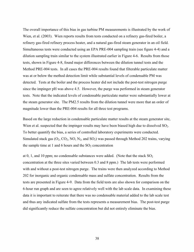
The overall importance of this bias in gas turbine PM measurements is illustrated by the work of

Wien, et al. (2003). Wien reports results from tests conducted on a refinery gas-fired boiler, a

refinery gas-fired refinery process heater, and a natural gas-fired steam generator in an oil field.

Simultaneous tests were conducted using an EPA PRE-004 sampling train (see figure 4-4) and a

dilution sampling train similar to the system illustrated earlier in Figure 4-6. Results from those

tests, shown in Figure 4-8, found major differences between the dilution tunnel tests and the

Method PRE-004 tests. In all cases the PRE-004 results found that filterable particulate matter

was at or below the method detection limit while substantial levels of condensable PM was

detected. Tests at the boiler and the process heater did not include the post-test nitrogen purge

since the impinger pH was above 4.5. However, the purge was performed in steam generator

tests. Note that the indicated levels of condensable particulate matter were substantially lower at

the steam generator site. The PM2.5 results from the dilution tunnel were more that an order of

magnitude lower than the PRE-004 results for all three test programs.

Based on the large reduction in condensable particulate matter results at the steam generator site,

Wien et al. suspected that the impinger results may have been biased high due to dissolved SO2.

To better quantify the bias, a series of controlled laboratory experiments were conducted.

Simulated stack gas (O2, CO2, NO, N2, and SO2) was passed through Method 202 trains, varying

the sample time at 1 and 6 hours and the SO2 concentration

at 0, 1, and 10 ppm; no condensable substances were added. (Note that the stack SO2

concentration at the three sites varied between 0.3 and 8 ppm.) The lab tests were performed

with and without a post-test nitrogen purge. The trains were then analyzed according to Method

202 for inorganic and organic condensable mass and sulfate concentration. Results from the

tests are presented in Figure 4-9. Data from the field tests are also shown for comparison on the

6-hour run graph and are seen to agree relatively well with the lab scale data. In examining these

data it is important to reiterate that there was no condensable material added to the lab scale test

and thus any indicated sulfate from the tests represents a measurement bias. The post-test purge

did significantly reduce the sulfate concentration but did not entirely eliminate the bias.

38

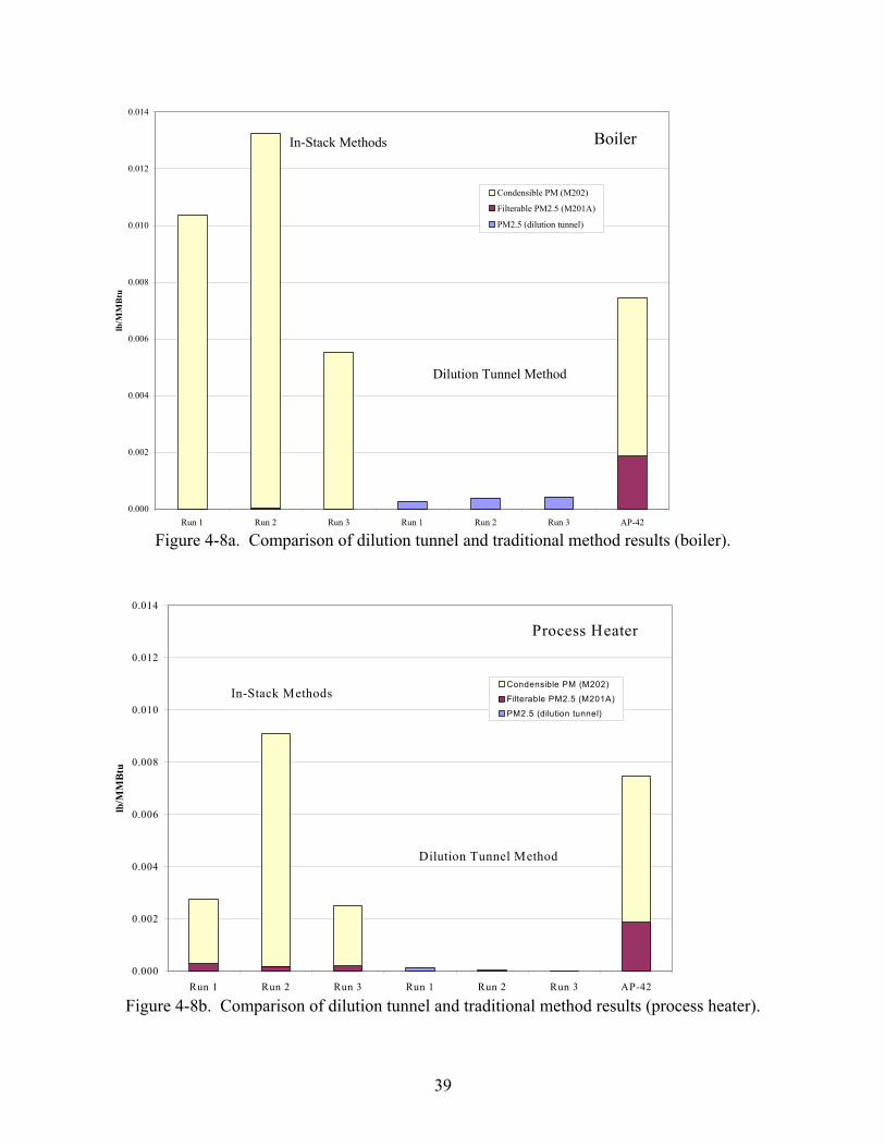
0.000

0.002

0.004

0.006

0.008

0.010

0.012

0.014 lb

/MM

Btu

Condensible PM (M202)

Filterable PM2.5 (M201A)

PM2.5 (dilution tunnel)

In-Stack Methods

Dilution Tunnel Method

Boiler

Run 1 Run 2 Run 3 Run 1 Run 2 Run 3 AP-42

Figure 4-8a. Comparison of dilution tunnel and traditional method results (boiler).

0.000

0.002

0.004

0.006

0.008

0.010

0.012

0.014

lb/M

MB

tu

Condensible PM (M202)

Filterable PM2.5 (M201A)

PM2.5 (dilution tunnel)

Process Heater

In-Stack Methods

Dilution Tunnel Method

Run 1 Run 2 Run 3 Run 1 Run 2 Run 3 AP-42

Figure 4-8b. Comparison of dilution tunnel and traditional method results (process heater).

39

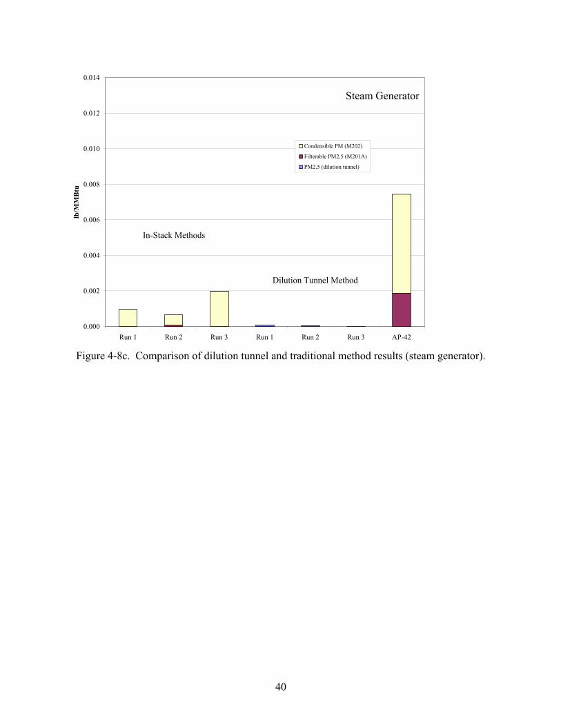
0.000

0.002

0.004

0.006

0.008

0.010

0.012

0.014 lb

/MM

Btu

Condensible PM (M202)

Filterable PM2.5 (M201A)

PM2.5 (dilution tunnel)

Steam Generator

In-Stack Methods

Dilution Tunnel Method

Run 1 Run 2 Run 3 Run 1 Run 2 Run 3 AP-42

Figure 4-8c. Comparison of dilution tunnel and traditional method results (steam generator).

40

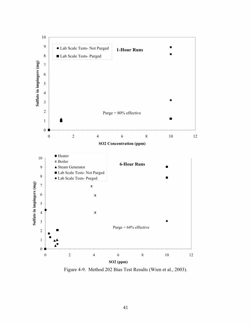
0

1

2

3

4

5

6

7

8

9

10Su

lfate

in im

ping

ers (

mg)

Lab Scale Tests- Not Purged

Lab Scale Tests- Purged

Purge = 80% effective

1-Hour Runs

0 2 4 6 8 10

SO2 Concentration (ppm)

0

1

2

3

4

5

6

7

8

9

10

Sulfa

te in

impi

nger

s (m

g)

Heater Boiler Steam Generator Lab Scale Tests- Not Purged Lab Scale Tests- Purged

6-Hour Runs

Purge = 64% effective

0 2 4 6 8 10

SO2 (ppm)

Figure 4-9. Method 202 Bias Test Results (Wien et al., 2003).

12

12

41

The purge was considerably less efficient for the 6-hour runs than for the 1-hour runs, indicating

that significant SO2 oxidation occurs in that time frame. Even though the amount of SO2

absorbed into the impingers may be small, the resulting bias is significant due to the already low

particulate emissions coming from gas-fired sources. Based on the above-described data, Wien et

al., suggest that condensable PM emissions data collected with EPA Method 202 may be

significantly biased.

Sample Analysis (Laboratory Procedures)

When the various sample fractions arrive at the analytical laboratory they must first be logged in

to maintain a chain of custody. The analytical procedures for the various fractions are described

below:

Probe Rinse. The acetone based probe rinse is contained in either a glass beaker or a Teflon®

baggie. The acetone is evaporated to dryness and then weighed. The mass of the residue

(determined as the tare weight) is considered part of the filterable particulate matter.

Particulate Filter. The filter must first be desiccated to remove any moisture absorbed by the

filter during sampling, recovery or in transit. The filter is then weighed to an accuracy of ± 0.5

mg.

Impinger Catch. The impinger catch is transferred to a distillation flash. Then methylene

chloride is added to the liquid and the mixture shaken. The water and methylene chloride will

separate into two layers, allowing the methylene chloride layer to be drained from the bottom of

the flask. This process is repeated three times to assure complete separation of the catch into two

fractions. The methylene chloride fraction will contain any condensable organic PM while the

water fraction will contain condensable inorganics including sulfates.

Organic Fraction. The organic fraction is evaporated to dryness and the mass of residue

determined gravimetrically.

Inorganic Fraction. There are two options for analysis of the inorganic fraction. The first option

is to simply evaporate the fraction to dryness and to weigh the residue. That residue can then be

reconstituted in water and analyzed for sulfates and other ions using ion chromatography. The

42

second option is to evaporate the inorganic fraction to a volume of about 1 to 3 mL rather than to

complete dryness. This avoids potential loss of HCl or H2SO4 from the residue. The partially

dried liquid is then diluted with water and titrated with NH4OH to stabilize the H2SO4. The

stabilized mixture is then dried and weighed.

Reagent Blanks. Blanks for the acetone, water and methylene chloride used in the field are

driven to dryness and the residue weighed. These data are then used to blank correct the

measurement results.

Though involved, the major laboratory equipment needs for determining the mass of filterable

and condensable particulate matter are a highly accurate balance to weigh the various fractions

and an environmentally controlled laboratory space. Additional equipment is needed to

determine the sulfate content and to analyze the catch for metal content and speciation. The

balance should have measurement resolution of at least 0.1 milligram. Note that a 250 mL

beaker weighs approximately 100 grams and the weight of the beaker plus residue must be

determined to within ± 0.5 mg. Several other factors must be addressed to accurately and

precisely make this type gravimetric analysis. Small particles can easily pick up a static charge

causing the particles to lift from the filter. To solve this problem, most labs place a small

radioactive source in the immediate vicinity of the balance. This eliminates (or at least

minimizes) the static charge. A further precaution is to electrically ground both the balance

beam and the technician operating the balance.

The laboratory area itself must be appropriately configured. The area should have an isolated

ventilation system, provide a high level of dust control and provide control of both temperature

and humidity. The samples, particularly the filter will absorb moisture from the ambient air

influencing the accuracy of the gravimetric operations. Of particular concern is that the humidity

be approximately the same during the initial and final filter weighing.

Before leaving the laboratory analysis area, it is important to further address the sulfate issue.

Wien’s data strongly suggests that SO2 is being absorbed into the impinger catch where it is

oxidized to sulfate. If the sampling event was for an extended period (e.g., 6 hours per run),

significant levels of sulfate might be expected even if a post-test nitrogen purge is performed.

When the impinger catch samples are analyzed at the laboratory, how the water fraction is

43

processed will likely impact the final data. If that fraction is simply driven to dryness, a portion

of the H2SO4 will likely be lost. Conversely, including the stabilization step will conserve the

acid as part of the reported inorganic condensable particulate matter. Thus, it is expected that the

detailed steps used in the laboratory analysis will contribute significantly to the observed data

variability.

Quality Assurance/Quality Control

All of the above described measurement methods have accompanying quality Assurance/Quality

Control requirements. These procedures generally include provisions for periodic calibration of

the sampling and analytical hardware, for gathering and analysis of blanks, and for periodic

audits of the laboratories.

The major periodic calibration requirement for PM measurements includes calibration of the

meter boxes used in the sampling trains and calibration of the scales used for gravimetric

analysis. At least every 6 months, the dry gas meter and meter box on a sampling train must be

five point calibrated against known standards. In essence this QA/QC procedure is to assure the

accuracy of the measured volume of gas passing through the train during a sampling event. The

allowable deviation in this parameter is ± 5 percent. For the gravimetric analysis there are two

basic requirements. First the manufacturer must check the operation of the balance at once every

year. Additionally, accuracy of the balance must be assured as part of each analysis session

using class S weights. Here the balance is challenged with a calibrated standard in the general

range of the weight being determined. For example, if a 250 mL glass beaker is used for analysis

of the acetone rinse, the balance output should be using a 100-gram calibration standard.

Conversely, if a Teflon® beaker liner is used for the analysis, a 1 or 2 gram standard would be

used.

In addition to calibration procedures, the PM measurement methods such as PRE-004 and

Method 202 require several blanks to be gathered and sent to the laboratory for analysis. These

include blanks for acetone, water, and methylene chloride. These are the materials used for

charging the impingers and for rinsing the glassware during sample recovery. The objective is to

assure that trace contaminants in the reagents do not unduly contribute to the reported data.

Some groups may also require collecting a filter blank, but how data from analysis of that blank

44

is used is seldom, if ever defined. Accordingly, most testing groups do not include filter blanks

as part of their QA/QC program.

Finally, certified analytical laboratories are required to participate in routine audits of laboratory

procedures. Moreover, for most EPA Methods, EPA has developed audit samples containing

known concentrations of some key analyte. These audit samples are periodically sent to the lab

to determine the overall accuracy of results relative to the known standard. For PM

measurements, audit sample are not a routine portion of the QA/QC procedures although it is

possible to challenge the lab relative to sulfate, condensable organic, or condensable inorganic

measurement.

Data Reduction and Reporting

The preceding sections have described the processes involved with generating data on the

filterable and condensable PM loading from emission sources. As discussed, the raw data

includes several components. The various elements include:

• Volume of sample gas collected along with data on the sample temperature and ambient pressure.

• Data on the basic composition of the stack gases including sufficient information to determine the oxygen content of the sampled gas.

• Information from the impingers on the total mass of moisture contained in the sampled gas volume.

• Initial and final weight of the filter

• Weight of the residue in the acetone rinse.

• Weight of condensable organic material in the methylene chloride portion of the impinger catch

• Weight of condensable inorganic material in the water portion of the impinger catch

• Weight of residue in the water, acetone, and methylene chloride blanks.

The Methods define exactly how these data are to be used in determining the PM emissions from

a source. EPA Method PRE-004 and most other extractive methods allow the data to blank

corrected. Thus, the mass of residue in the acetone blank can be subtracted from the measured

45

mass of the residue in the probe rinse. Similar corrections are allowed for the two fractions of

the impinger catch.

The basic information on sample volume, flue gas major constituents, sample temperature, and

ambient pressure are used to correct the sample volume to standard temperature and pressure and

then to correct the data to a reference oxygen content in the stack. This is a straightforward

calculation process but is often a source of considerable data variability. Different industries in

the US have adopted their own definition for reference temperature and pressure. It is unusual to

assemble a large database, compiled using results reported in the literature and to have consistent

data reduction procedures used for the entire database.

Earlier discussion addressed the fact that loss of small filter fibers during the recovery process

can result in measurement of negative filter weight gain. Although this situation occurs

frequently in PM sampling for low PM emission sources, there are no defined procedures for

how such results should be treated during data reduction. Since a negative filter weight gain has

no physical significance, such results are conventionally reported as zero rather than as a

negative emission when summing results from different fractions of the sampling train.

However, this convention lends false credibility to the accuracy of the measurement method and

is probably at least part of the explanation for the non-normal characteristic of the available

database.

Two final data reduction issues might also contribute to the observed data variability. First is the

issue of how data outliers are handled. In most instances, the reported emissions are the average

of triplicate runs without regard for the possibility that one or more of the runs may represent an

outlier. Good field-test practice should include annotation of any problems encountered during a

sampling run but that practice is not universally followed. Moreover, notations of field issues

are often ignored when data are reported or transcribed from reports into large electronic

databases. Absent a valid reason to exclude experimental results, it is better statistical practice to

err on the side of including all results. The second issue that could potentially contribute to data

variability is existence of mathematical errors during data reduction. Historically, this has been a

significant issue with field test data but widespread use of computers has dramatically reduced

the frequency of such problems.

46

EXTERNAL FACTORS

Uncontrolled factors external to both the process and measurement systems might also have an

impact on measured emissions and the variability of results in the database. Several factors that

might influence the data include:

• Ambient air particulate matter concentration

• Ambient humidity

• Ambient air temperature

• Nearby sources and activities.

From this list, the external factors most likely to influence PM measurement results are the

ambient air particulate matter concentration and nearby sources and activities. Humidity and

temperature have a direct impact on NOx emissions from gas turbines but that parameter should

have only a small impact on measured PM emissions. Ambient temperature and humidity also

effects humans and thus might impact the attention given to important details of field-testing.

Such an impact is considered a low probability as a source for large variability observed in the

database.

Gas turbines consume large quantities of ambient air. As such, factors such as high ambient PM

loading or high ambient loading of condensable organic or inorganic compounds might influence

measurement results. Such factors are a likely contributor to high concentration tail on the

filterable particulate matter in the database (see discussion in Section 3.)

ALTERNATE MEASUREMENT APPROACHES

In recognition of SO2 absorption and sulfate sampling issue, some recent tests were performed

that attempted to remove the bias. PM emissions data was gathered from four F-class gas

turbines using the modified EPA Method 8 sampling train illustrated earlier in Figure 4-5. The

intended use for Method 8 sampling is to determine the concentration of SO2 and SO3 in flue gas.

It is an alternative to use of continuous emissions monitoring for measuring SOx emissions. The

SO2 is absorbed in the 80 percent isopropanol impinger and its concentration can be accounted

47

for in the analysis. Other condensable materials, including sulfates in the stack are absorbed in

the 3 percent hydroxide impingers.

Results from these tests exhibited several of the aspects discussed earlier including the fact that

several of the filterable particulate matter gravimetric analyses showed negative weight gain.

For current use those negative values were retained in the overall data analysis rather than being

reported a zero. Results from those tests are presented as a normal probability distribution plot

in Figure 4-10. By including the negative data points, the filterable particulate matter data

clearly follow a normal distribution pattern. If they had been reduced to zero or near zero, the

data would have had the same pattern seen earlier in figure 2-1. The condensable particulate

fraction also exhibits a pattern that conforms to a normal distribution but the data do have more

scatter than the filterable portion.

The use of modified measurement procedures such as Method 8 may allow the sulfate artifact

bias to be removed. However, a thorough assessment of this modified measurement procedure

for determining condensable PM has not been performed. Results of a test comparing Method

202 to Method 8 showed that the sulfate content of the impinger residues was comparable and

dominated the total condensable particulate mass, but Method 202 showed a slight amount of

other substances that Method 8 did not capture (Wien et al., 2004). The potential for the same

SO2 artifact potential in Method 202 and in Method 8 is acknowledged by the requirement for a

post-test purge of the impingers in Method 8. Thus, while a modified Method 8 procedure for

reducing the variation in condensable particulate emissions shows potential, there remain a

number of unresolved questions regarding its use. At this time, EPA does not accept Method 8

as an approved alternate method for demonstrating compliance with PM10 emission standards

and limits.

48

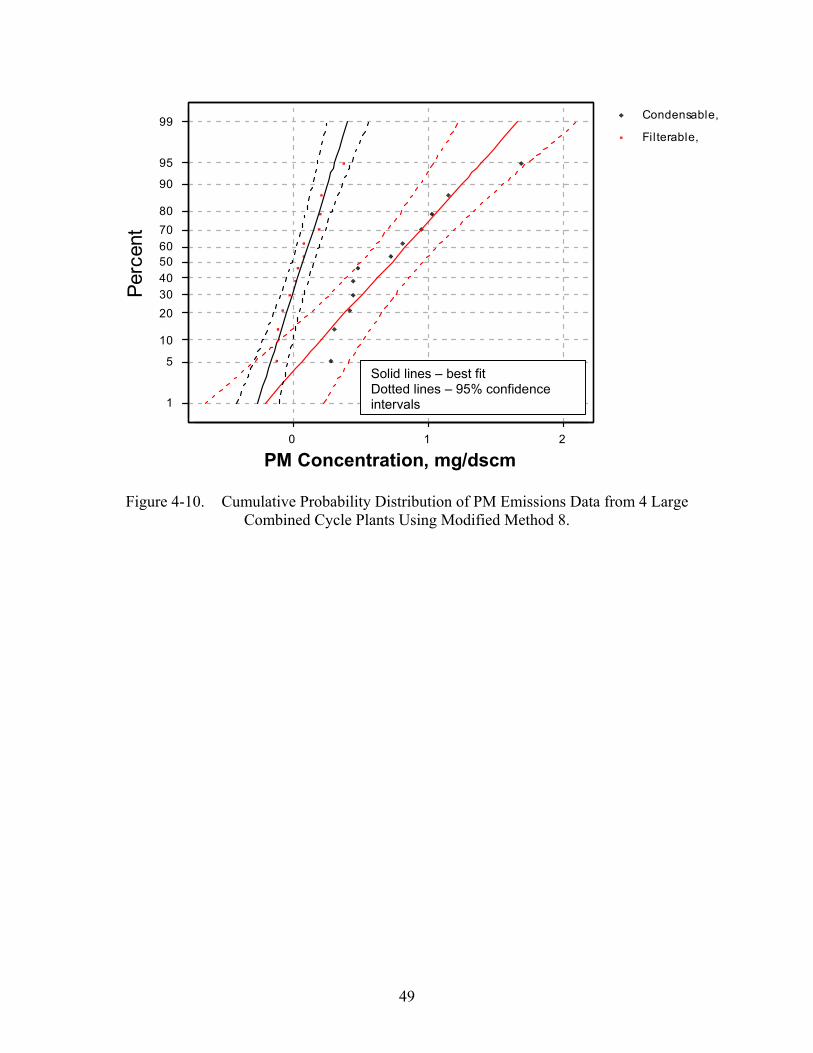
Data

Perc

ent

99

95

90

80 70 60 50 40 30 20

10

5

1

Solid lines – best fit Dotted lines – 95% confidence intervals

Condensable,

Filterable,

0 1 2

PM Concentration, mg/dscm

Figure 4-10. Cumulative Probability Distribution of PM Emissions Data from 4 Large Combined Cycle Plants Using Modified Method 8.

49

5. DISCUSSION

Available data describing PM emissions from gas turbine installations indicate wide variation in

the overall level of reported emissions. Analysis of the data shows that the variation does not

follow a normal distribution indicating that factors other than random variation contribute to the

observed data trends. Information presented in Section 4 examined a wide range of factors that

might contribute to data variability including gas turbine design features, system operating

factors, and the methods used to make source PM emission measurements. The current section

recaps the array of data variability drivers and provides a coarse ranking of the likely importance

of various factors. Within the scope of this effort, the factors considered are ranked on an

arbitrary scale of 1 to 5 (low to high importance).

It is noted that others may certainly have provided different relative rankings.

Results are summarized in Tables 5-1a and 5-1b addressing combustion equipment and

measurement considerations respectively.

Table 5-1a PM Variability Drivers – Equipment Considerations Factor Relative

Importance* Considerations

Turbine Size 2 Data should be segregated to separate very small units Fuel burned 3 Ash to filterable particulate matter and sulfur drives sulfate

artifact issue. Segregate data by gross fuel type Operating Cycle 2 Low temperature fired HRSG might increase carbonaceous PM

emissions Unit efficiency 1 Most emissions not directly related to relative quantity of fuel

consumed Inlet Air Filtration 3 Typical ambient air PM loading small relative to measured PM

exhaust emissions. Filters would likely remove large debris for filterable PM data.

Power Augmentation 2 Contaminants in water could be a large contributor to filterable and condensable inorganic PM

Combustor type 3 Carbonaceous PM emission impact SCR or Oxidation Catalyst Erosion

1 Age, maintenance condition

NH3 reagent water 1 Trace constituent in a low flow rate stream NH3 Slip 3 Collects in impingers and impacts artifact formation NO2 from oxidation catalyst

2 Nitrate artifact formation in impingers?

Equipment failure 1 *1=low importance, 5=high importance

50

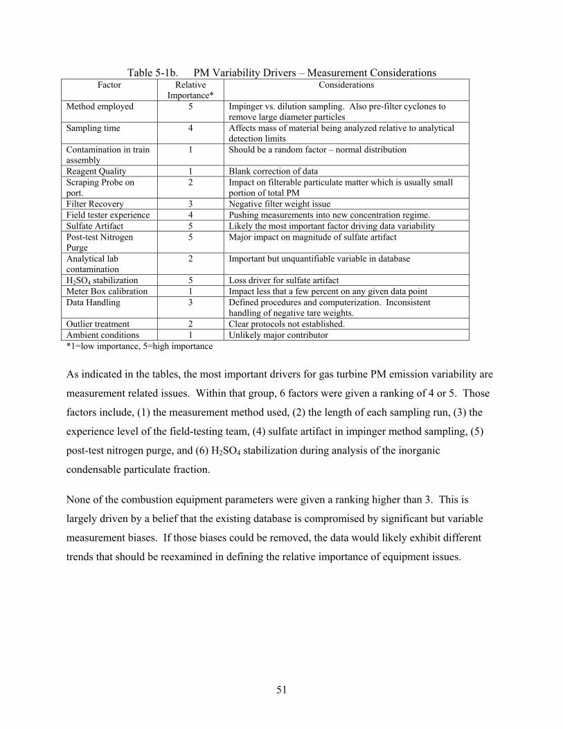
Table 5-1b. PM Variability Drivers – Measurement Considerations Factor Relative

Importance* Considerations

Method employed 5 Impinger vs. dilution sampling. Also pre-filter cyclones to remove large diameter particles

Sampling time 4 Affects mass of material being analyzed relative to analytical detection limits

Contamination in train assembly

1 Should be a random factor – normal distribution

Reagent Quality 1 Blank correction of data Scraping Probe on port.

2 Impact on filterable particulate matter which is usually small portion of total PM

Filter Recovery 3 Negative filter weight issue Field tester experience 4 Pushing measurements into new concentration regime. Sulfate Artifact 5 Likely the most important factor driving data variability Post-test Nitrogen Purge

5 Major impact on magnitude of sulfate artifact

Analytical lab contamination

2 Important but unquantifiable variable in database

H2SO4 stabilization 5 Loss driver for sulfate artifact Meter Box calibration 1 Impact less that a few percent on any given data point Data Handling 3 Defined procedures and computerization. Inconsistent

handling of negative tare weights. Outlier treatment 2 Clear protocols not established. Ambient conditions 1 Unlikely major contributor *1=low importance, 5=high importance

As indicated in the tables, the most important drivers for gas turbine PM emission variability are

measurement related issues. Within that group, 6 factors were given a ranking of 4 or 5. Those

factors include, (1) the measurement method used, (2) the length of each sampling run, (3) the

experience level of the field-testing team, (4) sulfate artifact in impinger method sampling, (5)

post-test nitrogen purge, and (6) H2SO4 stabilization during analysis of the inorganic

condensable particulate fraction.

None of the combustion equipment parameters were given a ranking higher than 3. This is

largely driven by a belief that the existing database is compromised by significant but variable

measurement biases. If those biases could be removed, the data would likely exhibit different

trends that should be reexamined in defining the relative importance of equipment issues.

51

6. FINDINGS

The key findings from this evaluation are summarized below:

• Mass emission measurements from gas-fired combustion turbines are highly measurement method dependent. Dilution tunnel methods report significantly lower emissions that traditional impinger train based methods.

• Traditional measurement methods probably overestimate the contribution of condensable particulate emissions due to the way in which condensation is driven in the train and existence of sulfate artifacts.

• Variation of filterable PM10 and PM2.5 emission measurements can be reduced by adding an in-stack cyclone on the probe inlet to remove spurious nonfuel and noncombustion related particles.

• Variation of condensable PM10 and PM2.5 emission measurements can be reduced by increasing the sampling time/volume and by modifying the impinger method to minimize SO4 artifacts by implementing a 30-minute post-test purge with nitrogen gas immediately following sample collection. Further investigation is needed to identify alternate impinger solutions for collecting condensable particulate matter that do not facilitate the sulfate (and possibly nitrate) artifacts.

• Dilution tunnel methods are feasible for gas turbine emission characterization; provide broader chemical speciation, better sensitivity, and direct comparability to ambient particulate matter measurement methods. Further investigation is needed to formally validate the measurement technique.

52

REFERENCES

Corio, L.A.; Sherwell, J. In-Stack Condensable Particulate Matter Measurements and Issues. J. Air & Waste Management Assoc. 2000, 50, 207-218.

DeWees, W.G.; Steinsberger, K.C.; Method Development and Evaluation of Draft Protocol for Measurement of Condensable Particulate Emissions; U.S. Environmental Protection Agency. U.S. Government Printing Office: Washington, D.C. 1990; EPA-450/4-90-012.

Filadelfia, E.J.; McDannel, M.D. Evaluation of False Positive Interferences Associated with the Use of EPA Method 202. Air and Waste Management Association 89thAnnual Meeting and Exhibition, Nashville, Tennessee, June 1996.

Hildemann, L.M.; Cass, G.R.; Markowski, G.R. (1989) A Dilution Stack Sampler for Organic Aerosol Emissions: Design, Characterization and Field Tests. Aerosol Sci. Technol. 1989, 10, 193-204.

Lanier, W.S. and Hendrix, C.D. (2001), Reference Method Accuracy and Precision (ReMAP), Phase 1, Precision of Manual Stack Emission Measurements, American Society of Mechanical Engineers, Research Committee on Industrial and Municipal Waste. (February, 2001.)

Linder, G. and S. Wall (1995). “Comparison of PAH emissions determined by ARB Method 429 and a dilution sampling (DS) method.” Unpublished presentation to Engineering Foundation Conference on Stationary Source Sampling and Analysis for Air Pollutants XIX, San Diego, CA (March, 1995).

Riley, G.R. and R. Myers, Comments From States That Require Method 202, International Conference on Stationary Source Sampling and Analysis for Air Pollutants XXVI, Destin, Florida, 2002.

SCAQMD, 2002. Method 5.2: Determination of Particulate Matter Emissions from Stationary Sources Using Heated Probe and Filter, District Source Test Manual, Monitoring & Source Test Engineering Branch, South Coast Air Quality Management District, Diamond Bar, California (2002).

U.S. Environmental Protection Agency. Federal Register, Volume 64. No. 189/Thursday, September 30, 1999/Rules and Regulations.

Wall, S.M. (1996) “Improved methods for PAH combustion source sampling.” Final Report, California Air Resources Board Contract A932-098, NTIS PB97148746.

Wien, S.E.; England, G.C.; Loos, K.R.; Ritter, K. Investigation of Artifacts in Condensable Particulate Measurements for Stationary Combustion Sources. Paper No. 536, 2003.

53

Wien, S.E., England, G.C., and Chang, M.C. 2004. “Development of Fine Particulate Emission Factors and Speciation Profiles for Oil and Gas-fired Combustion Systems, Topical Report: Test Results for A Combined Cycle Power Plant with Supplementary Firing, Oxidation Catalyst and SCR at Site Bravo,” GE Energy and Environmental Research Corporation, Irvine, CA.

54

Page: 29 [GCE1]Need reference for SCAQMD method, check that 5.2 is the right one.