development of comminution test method …jultika.oulu.fi/files/nbnfioulu-201710112973.pdf ·...
TRANSCRIPT
FACULTY OF TECHNOLOGY
DEVELOPMENT OF COMMINUTION TEST
METHOD FOR SMALL DRILL CORE SAMPLE
Hannu Heiskari
PROCESS ENGINEERING
Master’s thesis
September 2017

ABSTRACT
FOR THESIS University of Oulu Faculty of Technology Degree Programme (Bachelor's Thesis, Master’s Thesis) Major Subject (Licentiate Thesis)
Process engineering
Author Thesis Supervisor
Hannu Heiskari Saija Luukkanen, Professor.
Title of Thesis
Development of comminution test method for small drill core sample
Major Subject Type of Thesis Submission Date Number of Pages
Mineral processing Master’s thesis September 2017 82 p., 25 App.
Abstract
Grinding circuits are an essential part of a mineral processing plant. Grinding is very energy intensive, and can have
major effects on the following separation stages of mineral processing. This sets high requirements for the design
and operation of grinding circuits. Early on in the resource evaluation, ore samples used in metallurgical testing tend
to be composited samples from drill cores. These composited samples can have broad mineralogical variations in
them. Geometallurgy aims to create a predictive model to improve plant operation and design, based on the inherent
variability of ore blocks in an ore deposit. Thus to apply geometallurgy, mineralogical information and data about
the variability in ore blocks is essential. This creates a need for variability testing, where test methods are fast,
inexpensive and require low volumes of sample.
In this thesis the common Bond ball mill grindability test is conducted on three different sample materials. The
samples show good variability in terms of mineralogy and grindability. Along with the Bond test, the Mergan ball
mill grindability test is also conducted on the same sample materials. The Mergan test is faster than the Bond test,
and uses less sample material than the Bond test. The aim of the testwork is to analyze the differences between the
two test methods, and see if there is a correlation between them. This correlation can then be used to create a new
grindability test method, where the test is done with the Outotec Mergan mill, but the test results can be scaled to
estimate Bond work index for the sample.
Results show that there is indeed a correlation between the two grindability test methods. Using a linear model, an
experimental model is presented, where the Mergan mill can be used to approximate the Bond work index for an ore
with good correlation. To validate and improve the experimental model presented, more testing should be conducted
in the future.
Additional Information

TIIVISTELMÄ
OPINNÄYTETYÖSTÄ Oulun yliopisto Teknillinen tiedekunta Koulutusohjelma (kandidaatintyö, diplomityö) Pääaineopintojen ala (lisensiaatintyö)
Prosessitekniikka
Tekijä Työn ohjaaja yliopistolla
Hannu Heiskari Saija Luukkanen, professori.
Työn nimi
Development of comminution test method for small drill core sample
Opintosuunta Työn laji Aika Sivumäärä
Rikastustekniikka Diplomityö Syyskuu 2017 82 s., 25 liitettä
Tiivistelmä
Jauhatuspiirit ovat tärkeä osa rikastamoa. Jauhatus vaatii erittäin paljon energiaa, ja sillä voi olla merkittäviä
vaikutuksia rikastuksen seuraaviin osaprosesseihin. Tämä asettaa korkeat vaatimukset jauhatuspiirien suunnittelulle
ja käytölle. Malmiesiintymän tutkimuksen varhaisissa vaiheissa metallurgiseen tutkimukseen saatavat näytteet ovat
yleensä komposiittinäytteitä kairasydämistä, joissa voi olla suuria mineralogisia eroja. Geometallurgian
tarkoituksena on luoda ennustava malli, joka perustuu malmiesiintymässä olevien eri malmioiden eroavaisuuksiin.
Tätä mallia voidaan käyttää kaivoksien suunnittelun ja toiminnan optimoimiseen. Geometallurgian hyödyntämiseen
tieto malmioiden eroavaisuuksista ja mineralogiasta on siis välttämätöntä. Tämä on saanut aikaan tarpeen
testimenetelmille, joilla tätä vaihtelevuutta voidaan testata, ja näiden testimenetelmien tulee olla nopeita, halpoja, ja
testien käyttämien näytemäärien täytyy olla pieniä.
Tämän työn kokeellisessa osuudessa yleistä Bondin kuulamyllyjauhautuvuustestiä käytetään kolmen eri
malminäytteen jauhautuvuuden testaamiseen. Työssä käytettävät malminäytteet eroavat toisistaan paljon niin
mineralogian kuin jauhautuvuudenkin puolesta. Samojen näytteiden jauhautuvuutta testataan myös Mergan
kuulamyllyjauhautuvuustestillä. Mergan menetelmän etuja ovat Bondin testiin verrattuna se että Mergan on
nopeampi tehdä, ja sen näytevaatimus on Bondin testiä pienempi. Koetoiminnan tarkoituksena on verrata näiden
kahden jauhautuvuustestien tuloksia ja eroavaisuuksia, ja analysoida löytyykö näiden testimenetelmien väliltä
korrelaatiota. Tätä korrelaatiota voidaan sitten käyttää uuden jauhautuvuustestin kehittämiseen, jossa näytteen
jauhautuvuuden testaamiseen käytetään Outotecin Merganmyllyä, ja saatu tulos skaalataan Bondin ”työindeksiin”.
Koetulosteen perusteella jauhautuvuustestien väliltä löytyi korrelaatio. Tätä korrelaatiota käytetään kokeellisen
lineaarisen mallin luomiseen, jossa malmin jauhautuvuutta voidaan testata Merganmyllyllä ja arvioida siitä Bondin
”työindeksi” hyvällä korrelaatiolla. Kokeellisen mallin toimivuuden vahvistamiseen ja parantamiseen tarvitaan
kuitenkin vielä lisää testejä tulevaisuudessa.
Muita tietoja

FOREWORD
This thesis was written as an assignment under the supervision of Outotec Oy and
University of Oulu. The testwork and writing of this thesis was done between March and
September of 2017, in the city of Pori.
First of all, I would like to express gratitude for Outotec Oy and University of Oulu for
allowing me the chance to write this thesis. I would like thank my supervisors from
Outotec, Jussi Liipo and Harri Lehto for their help and guidance. From the University of
Oulu, I would like to thank my supervisors, Professor Saija Luukkanen and Maria Sinche
Gonzales (PhD, Eng.) for their knowledge, advice and support in writing of this thesis. I
would also like to express my gratitude to Pekka Kurki from Outotec Research Center
Pori, who taught me the all the procedures for this thesis, and for answering all my
questions and helping me whenever it was needed. Also thanks to all the people at ORC,
who made the great work environment I had the chance to be a part of, and for all their
help I got during my time there. I feel that this journey has increased my knowledge
immensely, but I still have so much more to learn.
I would also like thank my family and friends for their support during my studies in
university. Special thanks to my girlfriend Kaisa for all the support she has given me
during this project, which is the single most challenging thing I have ever faced. Without
every single one of you, this wouldn’t have been possible.

TABLE OF CONTENTS
ABSTRACT
TIIVISTELMÄ OPINNÄYTETYÖSTÄ
FOREWORD
TABLE OF CONTENTS
TERMS AND ABBREVATIONS
1 INTRODUCTION ......................................................................................................... 7
2 GRINDABILITY FUNDAMENTALS ......................................................................... 9
2.1 Basics ...................................................................................................................... 9
2.2 Particle breakage mechanics ................................................................................. 12
2.3 Mill power draw .................................................................................................... 15
2.4 Comminution theory ............................................................................................. 17
3 GEOMETALLURGY CONTEXT .............................................................................. 19
4 GRINDABILITY TEST METHODS .......................................................................... 24
4.1 Bond test................................................................................................................ 24
4.2 Mergan method ..................................................................................................... 27
4.3 Geometallurgical Comminution Test (GCT) ........................................................ 31
4.4 Wet Bond mill test ................................................................................................ 34
4.5 New Size Ball Mill (NSBM) ................................................................................. 36
4.6 Rapid determination of the Bond Work Index ...................................................... 37
4.7 Work index from field measurable rock properties .............................................. 40
5 TESTWORK, METHODS AND EQUIPMENT ......................................................... 45
5.1 Samples used ......................................................................................................... 45
5.2 Sample preparation ................................................................................................ 47
5.3 Bond tests .............................................................................................................. 53
5.4 Mergan tests .......................................................................................................... 56
6 RESULTS AND ANALYSIS ...................................................................................... 61
6.1 Bond tests .............................................................................................................. 61
6.2 Mergan tests .......................................................................................................... 65
6.3 Comparison between Bond tests and Mergan tests ............................................... 68
7 CONCLUSIONS .......................................................................................................... 77
8 FUTURE TESTWORK ............................................................................................... 79
9 REFERENCES ............................................................................................................. 80
10 APPENDICES ........................................................................................................... 83

TERMS AND ABBREVATIONS
AG autogenous grinding
b the representative diameter of the particles [m]
C constant, which depends on the material and comminution method
[kWh/t]
D diameter [m]
D80 80% passing size [µm]
d diameter of ball [m]
E energy
E0 energy used in Mergan grinding [kWh/t]
e coefficient of restitution of the material of the balls and mill
F80 80% passing size in the feed [µm]
Gbp ball mill grindability [g/rev]
g acceleration due to gravity [m/s2]
h height [m]
J volume occupied by charge [m3]
K constant chosen to balance the units of the equation
k constant, used to calculate Wi,GCT [kWh/t]
k grinding rate constant
L length [m]
M weight of the mill feed [g]
Md dry mass [g]
Mi index related to the breakage property of the ore [kWh/t]
M-Wi Mergan work index
Ms saturated-surface-dry mass [g]
MSO massive sulphide ore
m weight of the under-size [g]
N speed of rotation [m/s], [rev/min]
N total number of mill revolutions
Nc total number of mill revolutions giving the (2.5/3.5)M test sieve over-size
n mill revolutions per minute
n number of impacts
P power [W], [Nm/s]

P1 sieve opening at which test is carried out [µm]
P80 80% passing size in the product [µm]
PLI point load index
PSI Protodyakanov’s strength index
R test-sieve over-size [g]
R0 test-sieve over-size at the beginning of grinding [g]
R0 proportion of test sieve over-size in the new feed
RGO refractory gold ore
RHN rebound hardness number
RQD rock quality designation
SAG semi-autogenous grinding
T measured torque [Nm]
t grinding time [s]
tc grinding time in a standard grinding cycle after which the over-size (R)
on the test sieve is (2.5/3.5)M, which corresponds to the 250% circulating
load
U volume of liquid in pulp
U weight of the new feed [g]
V volume [m3]
W work [J]
Wi work index, material specific parameter which expresses the resistance of
the material to crushing and grinding [kWh/t]
Wi,MP Mergan predicted Bond work index [kWh/t]
W74 energy consumption per ton of -74 µm material produced [kWh/t]
x particle size [µm]
xf feed particle size [µm]
xp product particle size [µm]
𝜂 mill drive and engine efficiency
ρ density [t/m3]
ρw density of water [t/m3]
υ kinematic viscosity [m2/s]
σ effective density
λ geometric scaling factor

7
1 INTRODUCTION
Grinding, the last stage of the comminution process, is the most energy-intensive
operation in mineral processing, and can account for more than 50% of the operation cost
of a mineral processing plant. The purpose of grinding is the economic degree of
liberation of the mineral of interest. (Wills & Finch, 2015) Therefore, knowledge of a
given ore’s comminution properties are essential when operating a mineral processing
plant, or when conducting a feasibility study.
Comminution theory is concerned in the relationship between energy input into
comminution and the product particle size distribution made from a given feed size.
Grindability tests aim to estimate the energy consumption of grinding and to give
parameters for the sizing of the grinding mill using different test methods. The Bond test,
although an industry standard, can require up to 10 kg of sample material, and is rather
time consuming. (Bond, 1961a)
In the early stage of resource evaluation, when physical access and knowledge of an ore
deposit is limited or evolving, only drill core based samples are available for metallurgical
testing. Therefore, commonly samples collected for the testing are composite samples
representing a broad mineralogical variation within them. This hinders the detailed
mapping of ore variability using drill core samples. However, in the geometallurgy
context, mineralogical information is essential for creating a proper ore block model that
takes into account the inherent variability in the ore. Geometallurgical information is
essential in production planning and management, along with process control of the
resource’s exploitation before and during production. (Walters, 2008)
Geometallurgical approach to metallurgical testing has been under rapid research and
development in the recent years. Tests used in geometallurgical mapping must be fast,
inexpensive, and required ore sample must be small. Therefore, a fast grindability test
method that uses less sample material than the Bond test is required. In this thesis, a new
laboratory test method is developed. The aim of this test method is to use the Outotec
Mergan mill for the grindability test, and scale the results to the Bond ball mill test. The

8
Outotec Mergan method is faster than the Bond ball mill test, and requires less sample
material. However, the Mergan method gives grinding energy consumption, which can
be used to calculate Mergan work index, but this Mergan work index differs from the
Bond work index. Therefore, it is needed to analyze if the Mergan work index correlates
with Bond work index. All the testwork was conducted using Outotec Mergan and Bond
ball mills at Outotec Research Center, located in the city of Pori, Finland.
The literature review of this thesis focuses on basics of grindability, along with
geometallurgy, and presents various grindability test methods. In the experimental part of
this thesis, Bond ball mill tests and Mergan tests are done for 3 different ore samples, and
the results of these tests are analyzed. A new experimental model is represented, where
the Mergan test can be used to estimate the Bond work index of a specific ore.

9
2 GRINDABILITY FUNDAMENTALS
2.1 Basics
Most valuable minerals are often finely disseminated and intimately associated with the
gangue minerals, and thus they must be initially liberated before separation can be done.
This liberation is achieved by comminution, in which the particle size of the ore is
progressively reduced until the clean particles of the valuable mineral can be separated
from the gangue minerals by following separation processes. Grinding, the last stage of
comminution process, where particles are reduced in size by both impact and abrasion is
carried out until the mineral and gangue are produced as separate particles. When an
adequate amount of the mineral of interest is separated by comminution from the parent
rock, that size is usually known as the liberation size. (Wills & Finch, 2015; Gupta &
Yan, 2006)
Grinding is carried out either dry, or more commonly in suspension in water. It is
performed in cylindrical steel vessels that contain a charge of loose crushing bodies,
called the grinding medium. The grinding medium is free to move inside the mill, thus
comminuting the ore particles. Grinding mills are generally classified into two types,
tumbling mills and stirred mills. In tumbling mills, the mill shell is rotated and motion is
imparted to the charge via the mill shell. This movement is illustrated in Figure 1. The
grinding medium may be steel balls, steel rods, or rock itself (AG/SAG). Tumbling mills
are typically employed in primary grinding, typically reducing particles in size to between
25 and 300 µm. In stirred mills, the mill shell is stationary mounted either horizontally or
vertically, and motion is imparted to the charge by the movement of an internal stirrer.
Stirred mills find application in fine (15-40µm) and ultrafine (<15µm) grinding. (Wills &
Finch, 2015)

10
Figure 1. Trajectory of grinding media in tumbling mill. Modified from the source.
(Wills & Finch, 2015)
All ores have an economic optimum particle size in respect of following process stages.
If the ore is ground to too coarse particle size, insufficient mineral liberation limits
recovery in the separation stage. On the other hand, grinding the mineral to too fine
particle size increases grinding costs and may reduce final recovery. Thus efficient
grinding can be considered a key element to good mineral processing. (Wills & Finch,
2015)
Grinding costs are driven by energy and steel consumption. In some cases extensive
grinding may not be a disadvantage, as the increase in energy consumption may be offset
in the following processes. Although the economic degree of liberation is the principal
purpose of grinding, grinding is sometimes used to increase mineral surface area. As an
example of such processes, grinding of an industrial mineral such as talc is aimed at a
particle size that meets customer requirements. Another example would be grinding of
gold-ore, when extraction is made with hydrometallurgical methods, such as cyanide
leaching, where larger surface area improves cyanide leaching rate. (Wills & Finch, 2015)
11
Grinding is the most energy intensive operation in mineral processing. Although tumbling
mills have been developed to a high degree of mechanical efficiency and reliability, their
energy efficiency remains an area of debate. The greatest problem in tumbling mills, and
all crushing and grinding machines for that matter, is that the majority energy input is
absorbed by the machine itself, and only a small fraction of energy input is available for
breaking the ore. Wills and Finch (2015) state that “in a ball mill, for instance, it has been
shown that less than 1% of the total energy input is available for actual size reduction,
the bulk of the energy being utilized in the production of heat.” Also, plastic material will
eat up energy while changing shape, but will then retain this shape without actually
creating significant new surface. (Wills & Finch, 2015)
The breakage of the ore is mostly the result of repeated, random impact and abrasion. At
the present, there is no way that these impacts can be directed at the interfaces between
the mineral grains. Technologies such as microwave heating and high voltage pulsing are
currently used as an assisted breakage mechanic in grinding processes, not as the main
grinding process. (Wills & Finch, 2015) Another example would be high pressure roller
mill that can offer savings in comparison to traditional comminution circuits, while well
accepted in the cement industry, hasn’t yet seen much use in the mineral processing
industry (Mörsky, et al., 1995).
Metal wear is usually the second largest single item of expense in conventional grinding,
and in wet grinding installations it may approach or even exceed the power cost. The
kilograms of metal worn away and scrapped as worn parts varies with the abrasiveness
of the ore and the abrasion resistance of the metal. Metal wear is commonly expressed in
kg/ton crushed or ground. However, variations in feed, product sizes and in work index
are eliminated by expressing metal consumption as kg/kWh. (Bond, 1961b) This is one
area where autogenous and semi-autogenous mills have an advantage over traditional
mills that use other grinding media than the ore.
The purpose of mining and following beneficiation processes is to create a saleable
product, concentrate. Concentrate is a product, higher in the grade of mineral of interest,
than the ore being fed into the mineral processing circuit. Some industrial applications

12
such as aggregate production aim their comminution process at the size reduction of rock
to a specified particle size to create a saleable product. (Lynch, 2015)
The purpose of comminution circuit in mineral processing is to prepare the ore as a
suitable feed for separation processes. Separation processes upgrade the material by
rejecting the particles that do not contain economic amounts of the target mineral. The
implication is that the comminution process changes the ore from a population of particles
with a relatively uniform grade to particles with a range of compositions that allow them
to be separated into high-grade and low-grade streams. This so called mineral liberation
is a phenomenon, where according to Lynch (2015) “parent particles with a given
mineral composition break into progeny particles with a range of mineral compositions”,
is illustrated in Figure 2. (Lynch, 2015)
Figure 2. A simple representation of mineral liberation during breakage. Modified from
the source. (Lynch, 2015)
2.2 Particle breakage mechanics
Most minerals are crystalline materials in which the atoms are regularly arranged in three-
dimensional arrays. The configuration of atoms is determined by the size and types of
physical and chemical bonds holding them together. In the crystalline lattice of minerals,
these inter-atomic bonds are effective only over small distances, and can be broken if
extended by a tensile stress, such generated by tensile or compressive loading. Even when

13
rocks are uniformly loaded, the internal stresses are not evenly distributed, as the rock
consists of a variety of minerals dispersed as grains of various sizes. The distribution of
stress depends upon the mechanical properties of the individual minerals, but more
importantly upon the presence of cracks and flaws in the matrix, which act as sites for
stress concentration. The theories of comminution assume that the material is brittle,
however, crystals can store energy without breaking, and release this energy when the
stress is removed. Such behavior is known as elastic. (Wills & Finch, 2015)
The physical properties of the rock, e.g. shape and size, mainly determine the breakage
characteristics of an ore. According to Norazirah et al. (2015) “the shape properties are
increasingly being recognized as an important parameter influencing the performance
particles in mineral processing operations.” The characterization of the breakage process
can be done in two basic functions. The first one is the “selection function that represents
the fractional rate of breakage of particles in each size class” and the second one is “the
breakage function that gives the average size distribution of the daughter fragments
resulting from primary breakage event”. (Norazirah, et al., 2016)
When analysis is done to the breakage distribution of particle breakage, single particle
breakage characterization test methods are commonly used by researchers. They are
commonly grouped into three categories; single impact, double impact and slow
compression. The use of these tests is in input energy-size reduction relationships, based
on energy utilization. This can be grouped in to two categories. First is a drop weight test.
In a drop weight test a particle is resting on a hard surface, and is then struck by a falling
weight. The second type, known as a pendulum test, can give additional information on
the energy utilization in single particle breakage tests. (Norazirah, et al., 2016)
Even when a single particle is considered, the breakage event cannot be totally predicted
because of the large amount of variables that affect the outcome. Thus, to understand
particle breakage process, the focal point must be on the strength of the particle, the
energy consumed in the particle breakage event and the size distribution of the daughter
fragments yielded in the breakage event. When a particle’s theoretical strength is
considered, the assumption is that the particle is homogenous. In reality, there are always
flaws present in particles as lattice faults, grain boundaries and microcracks. These flaws

14
have much greater stress concentrations than the other parts of the particle. Thus fracture
initiates usually from these points, and in reality, the strength of the particle is lower than
the theoretical strength due to these flaws. (Fuerstenau & Han, 2003)
Obviously, commercial level comminution processes do not break particles one by one.
To process ores at a commercial level, up to thousands of tons of ore per hour,
comminution devices must obviously break huge assemblies of particles. In reality,
comminution happens in multiparticle breakage event, and these events are more complex
and less efficient that single particle breakage events. This is because particles interact
with each other during multiparticle breakage. The general belief is that the amount of
breakage that occurs is dependent on how energy is dissipated in the process, either useful
or wasted. Efficiency of breakage is dependent on the number of particle layers
undergoing compression. As particle layers increase in number, the efficiency decreases.
(Fuerstenau & Han, 2003) Figure 3 illustrates the differences of a single-particle and
multiparticle breakage event in a compression breakage.
Figure 3. Illustration of single-particle and multi-particle breakage event. Modified from
the source. (Fuerstenau & Han, 2003)
The process of grinding an ore particle is dependent on the probability of the particle
entering an area between the grinding medium, and the probability that some breakage
event occurs when the particle is in the area. Size reduction can be achieved by several
different mechanisms, such as impact or compression due to some sudden force being
applied to the particle surface, chipping or attrition due to steady compressing forces that
break the matrix of a particle, and due to abrasion (shear) where forces act parallel to, and

15
along the surfaces of the particles. These mechanisms cause deformations in the particles,
changing their shape beyond certain limits, which then causes them to break. These
mechanisms are illustrated in Figure 4. (Wills & Finch, 2015)
Figure 4. Mechanisms of breakage: (a) Impact or compression, (b) Chipping or attrition,
and (c) Abrasion. Modified from the source. (Wills & Finch, 2015)
Modern day comminution uses research methods such as DEM (Discrete Element
Method) to predict the flow of the particulates and to simulate the different multiparticle
breakage events inside the mill. Since grinding is inherently a process involving collisions
between particles and the mill itself, methods to analyze the size reduction happening
inside the mill, and their effect on mill performance is a topic of heavy investigation.
(Cleary & Morrison, 2016)
2.3 Mill power draw
The power required to drive a tumbling mill depends to some extent on every one of the
physical dimensions defining the mill shell and ball charge, and on many of those defining
the properties of the ore charge. The power to drive the mill, P, would be expected to
depend upon the length of the mill, L, the diameter, D, the diameter of ball, d, the density
of the ball, ρ, the volume occupied by the charge (including voids) expressed as a fraction
of the total mill volume, J, the speed of rotation, N, the acceleration due to gravity, g, the
coefficient of restitution of the material of the balls and mill, e. (Rose & Sullivan, 1958)

16
The power, P, would also be expected to depend upon the following characteristics of the
ore: the representative diameter of the particles, b, the energy necessary to bring about
unit increase in the specific surface of the ore, E, and the volume, V, occupied by the ore
charge (including voids) expressed as a fraction of the volume between the balls in the
mill. Furthermore, the power P would be expected to depends upon the effective
kinematic viscosity of the mixture of ore and fluid, υ, the effective density of the mixture,
σ, and in the case of wet milling, volume of the liquid in the pulp, U. Finally, when the
interior of the mill is fitted with lifters it would be expected that the power, P, would
depend on the number of lifters, n, and upon the height of the lifters, h. Thus, the power
can be expressed symbolically (1), when ϕ denotes some function of each of the quantities
within the bracket. (Rose & Sullivan, 1958)
P = ϕ(L, D, d, ρ, J, N, g, e, b, E, V, υ, σ, U, h, n) (1)
Calculations for the power requirements of a mill, from theoretical standpoint, are hard
to make. This is due to the fact that even a fairly complete theory on the internal dynamics
of a ball mill, where all of the aforementioned variables are given due importance, has
not been propounded. Due to the great number of variables, the analysis of the effect of
all these variables on the power draw of tumbling mills has been prohibitive for a
complete experimental study. (Rose & Sullivan, 1958) It is quite telling that in some
cases, things like catastrophe theory have been applied when investigating the inner works
of tumbling mills (Zhitie, 1995).
A common practice to estimate the power draw of a mill is as a function of the mill charge
motion. The problem of in situ characterization of charge motion is the aggressive internal
environment of tumbling mills, and models focus on empirical relationships of the effects
of the charge on the power draw, and the charge is usually simplified to a single bulk
body. While models have shown good approximation between the mill power draw and
the charge motion, they seem to be limited to the scope of their definition. Techniques
like PEPT (Positron Emission Particle Tracking) can be used to measure the flow
trajectory of radioactive particle in a granular or fluid system such as tumbling mills,
allowing for better modeling on the mill power draw as a function of the mill charge
movement. (Bbosa, et al., 2011)

17
2.4 Comminution theory
Comminution theory is interested in the relationship between the energy input in size
reduction, and the particle size made from a given feed size. Comminution theory expects
that a relationship can be found between the energy required to break the material, and
the new surface created in the comminution process. This relationship can only be made
manifest if the energy used in the creation of new surface can then be separately measured.
Many theories have been presented, but none seem completely satisfactory. All the
theories of comminution make the assumption that the material is brittle, and thus no
energy is adsorbed in the comminution process which is not finally utilized in ore
breakage. (Wills & Finch, 2015) The author of this thesis would like to note that, as
mentioned before, no comminution process is even remotely efficient enough that no
energy is wasted.
First and oldest theory of comminution was presented by Paul von Rittinger in 1867.
According to Rittinger’s law, the energy consumed by the comminution process is
directly proportional to the new surface area produced which is shown in equation (2). E
is the energy used in comminution, x is particle passing size and C is material dependent
constant. (Hukki, 1964)
𝐸 = 𝐶 (1
𝑥𝑝−
1
𝑥𝑓) (2)
Friedrich Kick presented his second theory in 1885, represented by equation (3), which
can be defined as “the energy required for producing analogous changes of configuration
in geometrically similar bodies of equal technological state varies as the volumes or
weights of these bodies”. According to Kick’s law, energy required for transformation is
proportional to mass or to volume of the particle. (Hukki, 1964)
𝐸 = 𝐶 ln (𝑥𝑓
𝑥𝑝) (3)

18
The third theory of comminution, presented in 1952 by Fred C. Bond, widely used in the
industry, assumes that the energy used in comminution is inversely proportional to the
square-root of the diameter of the particle as is shown in equation (4). (Hukki, 1964)
𝐸 = 2 𝐶 (1
√𝑥𝑝−
1
√𝑥𝑓) (4)
All of these three theories may be derived from the basic differential equation (5) created
by Walker, Lewis, McAdams and Gilliland in 1937. The energy required for comminution
grows as the particle size decreases, or in other words, fineness increases. Thus, all three
theories of comminution are usable on a specific range of particle size, Kick’s law on the
coarse size range of particle (crushing), Bond’s law on medium particle size (traditional
grinding), and Rittinger’s in fine grinding range. (Hukki, 1964)
𝑑𝐸 = −𝐶𝑑𝑥
𝑥𝑛 (5)
On the basis of Hukki’s evaluation, Morrell proposed in 2004 a modification to Bond’s
equation that relates specific energy to size reduction and the rock breakage properties
are assumed to be constant with respect to particle size. By designating Mi as a
comminution index, K as constant to balance the units of the equation, Morrell’s equation
can be expressed as (6). Morrell concluded that this new equation does not suffer from
the same deficiency as Bond’s equation, Bond’s equation being usable specifically on
medium particle size. (Morrell, 2004)
𝑊 = 𝑀𝑖𝐾(𝑥2𝑓(𝑥2)
− 𝑥1𝑓(𝑥1)
) (6)

19
3 GEOMETALLURGY CONTEXT
Growing demand for more efficient utilisation of orebodies and proper risk management
in mineral processing industry have emerged a new branch called geometallurgy.
Lamberg (2011) states that “geometallurgy combines metallurgical and geological
information to create spatially-based predictive model for mineral processing plants.”
According to Lamberg, geometallurgy is not a discipline itself, but related to certain ore
deposit and certain process, and as such geometallurgy can be called a practical
amalgamation of ore geology and mineral processing. A geometallurgical program should
go through an 8 step program, illustrated in Figure 5. (Lamberg, 2011)
Figure 5. Geometallurgical program in 8 steps. Modified from the source. (Lamberg,
2011)

20
According to Walters (2008) the discipline of geometallurgy is not new “but it is
becoming increasingly recognized as a discrete and high-value activity that reflects
ongoing commercial and cultural trend towards more effective mine site integration and
optimization.” The aim of geometallurgy is not replace existing approaches to design and
optimization of mining and mineral processing circuits, but rather to complement them.
(Walters, 2008)
The idea behind geometallurgy is to provide information that reflects inherent geological
variability of the ore, and impact of this variability on the metallurgical performance. To
achieve this, ore deposits need to be determined in terms of machine-based process
parameters, which include hardness, comminution energy, size reduction, liberation
potential and product recovery. These geometallurgical parameters can be used in
geostatistics to populate deposit wide block models. Incorporating these geometallurgical
parameters into operation of mineral processing plants supplements traditional geology
and grade-based attributes, which allows more comprehensive approach to economic
optimization of mining and mineral processing. (Walters, 2008)
Geometallurgy requires integration across a wide range of existing operations.
Geometallurgy can be described in various ways, including aspects of process
mineralogy, mine geology, metallurgy, process control, resource modeling and
geostatistics. Geometallurgy can also be called orebody knowledge or ore
characterization. (Walters, 2008)
The information about the inherent geological variability of the ore block can be used in
geometallurgical models to reduce technical risk when designing and operating mineral
processing plants. When considering feasibility before design phase, when physical
access to an ore deposit or knowledge about an ore deposit is limited and evolving,
geometallurgical approach becomes increasingly important. During design phase of a
plant, geometallurgical data can be used to optimize flow sheet design and equipment
sizing. Geometallurgical data is also useful when optimizing plant performance and
production during the whole life-cycle of the plant. (Walters, 2008)

21
The linkage of geological information and metallurgical response currently relies on a
limited number of samples tested in laboratory conditions. The weakest points in
geometallurgical programs are typically small number of test samples used in
metallurgical testing, and insufficient information collected from drill cores. In the
metallurgical testing samples are quite small both in terms of size and number, and the
samples should represent large tonnages of the ore. This sets high requirements for
sampling and testing, as samples tested should represent the full variability of the ore
block, and the metallurgical response of the ore. (Lamberg, 2011)
One problem with geometallurgical testing is the tendency to composite core-based
samples to represent larger scale production or to fulfill the logistical requirements of
physical testing procedures. Using composite samples that disguise natural variability and
are non-representative and unconstrained can cause significant problems, such as precise
test results with uncertain representativity. The ultimate engineering solution to
variability in the ore is to homogenize the feed over the life of the mineral processing
plant. However, homogenized ore feed might not represent a simple linear combination
of the ore, and it might not produce optimal economic outcomes. (Walters, 2008)
Before a final design is chosen, the variability of the ore and its effects on process
performance are important knowledge. Thus identifying the variability in the ore deposit
through geometallurgical methods allows increase in efficiency and optimization of the
mineral processing plant. This is especially true for large scale mining operations, which
have increasing potential to exploit ore variability through multiple processing circuits.
This can also help with improving overall sustainability and reduce energy costs and
environmental footprint of the mineral processing plant. (Walters, 2008)
One of the main drives behind rising application of geometallurgy is the desire to move
towards low cost physical testing. This allows using small sample volumes that can be
used to define natural variability in the ore. For geometallurgy, defining natural variety
with models built from large sets of data with small sample volumes is a much better
statistical approach, than building the models with small number of more precise test
samples. This approach results in a large number of low cost comparative tests to provide
22
information about the variability in the ore, and decrease the number of high precision
tests. (Walters, 2008)
Even a larger number of more spatially representative tests, when compared to the overall
volume of the ore deposit, still represent sparse data. Larger number of data sets does
partly overcome some of the problems with current approach, but to effectively use
geometallurgical processing information on ore deposit scale, statistical and population
modelling techniques are required along with classical geostatistics. (Walters, 2008)
To make the sampling, and also the definition of geometallurgical ore domains more
reliable, new measurement and analysis techniques are needed. The challenge is that tests
should be done for a very big number of samples, up to thousands, and as such the
techniques used must be fast, inexpensive and preferentially fully automated. The tests
can be roughly divided into three groups, tests measuring rock properties, tests for
quantitative mineralogy and geometallurgical tests. (Lamberg, 2011)
Another problem with using geometallurgy in grinding processes with current
grindability test methods is accuracy. The test method should be accurate over the entire
range of hardness variability for the entire ore deposit. For geometallurgical analysis,
every block in the ore deposit should be represented by a real test. (Starkey & Scinto,
2010)
The development of tests and methods for the geometallurgical modelling of ore blocks
has been under a rapid research and development in the recent years, e.g. the
Geometallurgical Comminution Test by Mwanga et al. (2017) which will be described in
chapter 4.3. The need for rapid, low cost testing of ore properties thus sets a need for
improving the Mergan test method (described in chapter 4.2) and topic of this research.
One case where modelling of ore domains lead to better production planning is Batu
Hijau, where Metso Mineral Process Technology and PTNNT Batu Hijau worked to
develop a model to forecast and optimize SAG mill throughput at the mineral processing
plant. Based on the ore characterization and the model created, better mill throughput
could be predicted. The ore domains were defined based on ore lithology, rock structure

23
(RQD) and rock strength (PLI). The model takes the ore through the whole comminution
circuit, starting from blasting and ending at grinding circuit. (Burger, et al., 2006)
Outotec’s vision on geometallurgical testwork is presented in Figure 6. For this vision the
Mergan ball mill test, presented in chapter 4.2, is a better grindability test than Bond test,
but the problem with the Mergan test is that it gives grinding energy consumption, which
can be used to calculate “Mergan work index” but this work index gives different values
than the Bond work index. This causes the need for the testwork in this thesis, to see if
there is correlation between the Mergan work index and Bond work index, and to develop
the Mergan method so that it can be used to give Bond work index values based on the
grinding energy consumption. The product of the Mergan test can also be used in
mineralogical and chemical analyses, and beneficiation tests.
Figure 6. Outotec’s geometallurgical testwork vision

24
4 GRINDABILITY TEST METHODS
Grindability test methods are used for determining the energy requirement when grinding
a product to a desired size. These methods vary depending on the mill type and
manufacturer. Mill designers typically use the Bond test and tests derived from Bond test
for sizing ball mills.
The Bond test, although an industry standard, is not without limitations. The test requires
specific preparation work for the sample, and usually can be used to determine
grindability to a rather slim range of particle size of the product. A single Bond test can
require up to 10 kg of sample material, and is rather time consuming, meaning it can take
a skilled technician up to 8 hours or more work for a single test.
Thus, in the geometallurgy context, the standard Bond test can be considered far too
demanding in terms of the amount of sample needed, as well as time consumed. This
makes the Bond test too expensive and inefficient to be used as a standard test for
geometallurgical mapping of ore deposits. Due to this, Bond test is used as a baseline in
this thesis, and the other test methods introduced are methods that are either variations of
Bond test to overcome the limitations of the Bond test, or can be considered
“geometallurgical” tests for ore comminution.
The Mergan test, along with the Bond ball mill test will be used in the experimental part
of this thesis. Mergan test can be done faster than the Bond test, and it only uses the
weight of 1500 cm3 of packed sample material. Thus, the Mergan test, if scalable to Bond,
is an improvement to Bond test in Outotec’s geometallurgy vision.
4.1 Bond test
According to Bond’s Third Theory, the work input is proportional to the new crack tip
length produced in particle breakage, and equals the work represented by the product
minus that represented by the feed. For practical calculations, if we designate the work
input in kilowatt hours per short ton as W, P80 as 80 percent product passing size in µm,
25
F80 as 80 percent feed passing size (µm) and Wi is designated work index, Bond’s basic
third theory (4) can be expressed as equation (7). Work index is a material specific
comminution parameter which expresses the resistance of the material to crushing and
grinding. (Bond, 1961a)
𝑊 =10𝑊𝑖
√𝑃80−
10𝑊𝑖
√𝐹80 (7)
If the material is homogenous to size reduction, its work index (Wi) value will continue
constant for all size reduction stages. However, heterogeneous rock structures are
common and for instance, certain materials have a natural grain size, and their Wi values
will be larger below that size than above it. The efficiency of the reduction machine may
also influence the work index. As an example, a ball mill grinding an ore from 80 percent-
14 mesh (1410 µm) to 80 percent-100 mesh (150 µm) will have a lower operating work
index value with 1.5 in grinding balls than with oversize 3 in balls. Laboratory
determinations of the work index show the resistance to breakage at the size range tested,
and any variation in the work index values in tests at different product sizes shows that
the material is not homogenous to size reduction. As such, laboratory tests should
preferably be made at or near the product size required in commercial grinding. (Bond,
1961a)
Bond has derived equations for finding the work index from several types of laboratory
crushability and grindability tests. For this thesis, Bond’s ball mill grindability test is the
most important, which will be described below.
The standard feed is prepared by stage crushing to all feed passing a 6 mesh (3350 µm)
sieve, but finer feed can be used when necessary. The feed is screen analyzed and packed
by shaking in graduated cylinder, and the weight of 700 cm3 is placed in the mill and
ground dry at 250 percent circulating load. The mill is 12 x 12 in, or 305 x 305 mm in
diameter with rounded corners, and a smooth lining except for a 4 x 8 in hand hole door
for charging. The mill has a revolution counter and runs at 70 rpm. The grinding charge
of the ball mill consists of 285 iron balls weighing 20.125 kg. The ball charge should
consist of about 43 1.45 in balls, 67 1.17 in balls, 10 1 in balls, 71 0.75 in balls, and 94

26
0.61 in balls with a calculated surface area of 842 sq. in. Tests can be made at all sieve
sizes below 28 mesh (600 µm). (Bond, 1961a)
The first grinding period is 100 revolutions, after which the mill is dumped, the ball
charge is screened out, and the 700 cm3 of material is screened on sieves of the mesh size
tested, with coarser protecting sieves if necessary. The undersize is weighed, and fresh
unsegregated feed is added to the oversize material to bring its weight back to that of the
original charge. Then the feed is returned to the ball mill and ground for the number of
revolutions calculated to produce a 250 percent circulating load, after which the material
is again dumped and rescreened. The number of revolutions required is calculated from
the results of the previous period to produce sieve undersize equal to 1/3.5 of the total
charge in the mill. (Bond, 1961a)
The grinding period cycles are continued until the net grams of sieve undersize produced
per mill revolution reaches equilibrium and reverses its direction of increase or decrease.
Then the undersize product and circulating load are screen analyzed, and the average of
the last three net grams per revolution, Gbp, is the ball mill grindability. When P1 is
designated as the opening of the sieve size tested (µm), then the ball mill work index Wi
is calculated from equation (8). (Bond, 1961a)
𝑊𝑖 =44.5
𝑃10.23×𝐺𝑏𝑝
0.82×(10
√𝑃80−
10
√𝐹80) (8)
It should be noted that the work index calculated in equation (8) is specific to short ton.
For calculating the work index in kWh/t, equation (9) should be used.
𝑊𝑖 =49.1
𝑃10.23×𝐺𝑏𝑝
0.82×(10
√𝑃80−
10
√𝐹80) (9)
The work index value from equation (8) should conform with the motor output power to
an average overflow ball mill of 8 ft. interior diameter in grinding wet closed circuit.
Bond also introduces correction multipliers, such as in dry grinding work input should be
multiplied by 1.30 and when D is mill diameter inside the lining in ft., the work input
should be multiplied by (8/D)0.2. (Bond, 1961a)

27
4.2 Mergan method
In 1970 Niitti developed a batch type grindability test method, which he named Mergan,
milling energy analyzer. According to Niitti, basic demands for a dependable grindability
test are:
- The energy consumption has to be measurable.
- The test must be performed either wet or dry corresponding with the industrial
grinding process.
- The test must be carried out to the same final fineness as the industrial grinding
process.
- The procedure of a test must be simple and rapid.
The measurements of the mill are 268 × 268 mm, corresponding to a 1/100 of a “base
mill”. The speed of the mill can be regulated within wide limits. The net energy
consumption of the mill is continuously determined by a simple but sensitive pendulum
type torque measurement from the mill axis. For ease of operation the mill is equipped
with a revolution counter switch, along with necessary aids for emptying the mill and
separation of the sample from the grinding media. (Niitti, 1970)
Niitti conducted a large series of tests to study the effect of various factors on the
grindability of the material, and to determine the optimal conditions for operating the
Mergan mill. The main material tested was the Outokumpu ore containing about 50
percent sulphides and 50 percent silicates. At first the optimum working conditions of the
mill were investigated by changing various factors so that the minimum energy
consumption per ton of new -74 µm material produced, W74, was found. (Niitti, 1970)
The optimum amount of grinding media, steel balls, is 22 kg, which fills almost half of
the mill. Figure 7 illustrates the effects of the amount of grinding media on optimum
working conditions. With a smaller ball charge the aforementioned energy consumption,
W74, increases rapidly. With a heavier ball charge the increase is quite small. Balls of
different sizes were also tested. Niitti found that a natural ball charge consisting of balls
between 15 and 40 mm was the most efficient, and was chosen as a standard. The

28
optimum amount of material is 1500 cm3, which in practice fills the interstitial spaces
between the balls. (Niitti, 1970)
Figure 7. Effects of the amount of grinding media on the batch mill optimum working
conditions. Modified from the source. (Niitti, 1970)
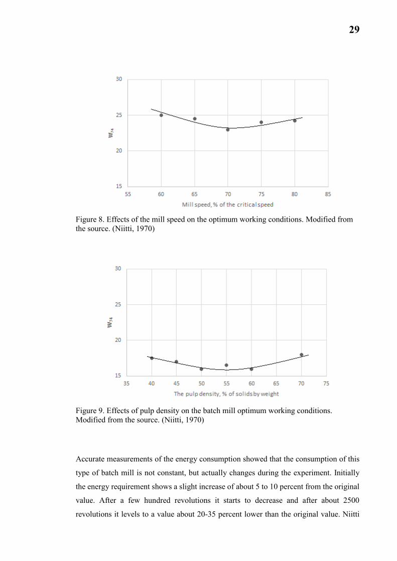
The optimum speed of the mill is 70 % of the critical speed of the mill shell. The optimal
pulp density in wet grinding 50 to 60 percent solids by weight. Both in case of the pulp
density and the mill speed, the increase in energy consumption is quite slow near optimum
values, as demonstrated in Figures 8 and 9. (Niitti, 1970)
29
Figure 8. Effects of the mill speed on the optimum working conditions. Modified from
the source. (Niitti, 1970)
Figure 9. Effects of pulp density on the batch mill optimum working conditions.
Modified from the source. (Niitti, 1970)
Accurate measurements of the energy consumption showed that the consumption of this
type of batch mill is not constant, but actually changes during the experiment. Initially
the energy requirement shows a slight increase of about 5 to 10 percent from the original
value. After a few hundred revolutions it starts to decrease and after about 2500
revolutions it levels to a value about 20-35 percent lower than the original value. Niitti

30
assumed that this decrease happened because of the change in the friction conditions in
the mill due to the decrease in grain size. Investigators tried to eliminate this phenomenon
by installing lifter bars in the mill, however, experiments indicated that this measure does
not eliminate the phenomenon. The aforementioned phenomenon is illustrated in Figure
10. (Niitti, 1970)
Figure 10. An illustration of net power alteration during grindability test. Modified from
the source. (Niitti, 1970)
The material ground also clearly affects the energy consumption of the mill. The energy
requirement for dry and wet grinding is quite different. In general, wet grinding is
distinctly more efficient than dry grinding, the difference being frequently 30-50 percent.
On basis of the facts mentioned above, Niitti concluded that it is not possible to determine
accurately the grindability of wet industrial process on the basis of a dry grinding test.
The determination must be carried out with the same medium as that with which the
grinding process will take place. (Niitti, 1970)
The finer the grinding product is the more difficult the grinding tends to become. This
difficulty varies with the material, thus, it is not feasible to describe the grindability with
a single figure or index, which would cover the whole range of grain sizes. For a test of
the grindability to be reliable, it must be carried out to the same fineness as the actual
process of grinding done. (Niitti, 1970)

31
When conducting a grindability test using the Mergan mill, the sample is to be crushed to
about -4 mm size. The fineness of the material is determined by a sieve and surface area
of the material by a rapid permeability analysis. Based on the data measured (E0) as
described, the grindability of the material tested can be calculated directly as energy
consumption in kWh/t when ground from a given initial fineness to a desired final
fineness. The grindability (W74) may be expressed as kWh/t of the new -74 µm material
produced, or as kWh/t per 1000 cm2/cm3 of the new specific surface area produced. The
grinding energy consumption (E0) can also be used to calculate M-Wi, or “Mergan work
index) according to equation (10). (Niitti, 1970; Kurki, 2006)
𝑀 − 𝑊𝑖 = 𝐸0 (√𝐹80
√𝐹80−√𝑃80) √
𝑃80
100 (10)
where M-Wi is Mergan work index [kWh/t]
E0 is energy consumption [kWh/t]
It should be also noted, that even though E0, W74 and Wi are all expressed as kWh/t, they
mean different things, and can cause some confusion. It is clear that when talking about
these grinding parameters, it has to be very specific that what the value stands for.
4.3 Geometallurgical Comminution Test (GCT)
Geometallurgical Comminution Test program, developed at Luleå University of
Technology, aims to provide a test method that is usable in analyzing even small drill
core samples. The program consists of crushability and grindability test work, along with
mineralogical analyses for entire samples as well as selected sieve fractions. Results from
the test program include modal mineralogy, particle size distributions, work indices and
mineral liberation analysis. (Mwanga, et al., 2017)
As a part of the test program, a small scale batch grindability test method has been created
as a shortcut for estimating Bond ball mill work index for the ore. This small scale
grindability test method uses a small laboratory ball mill, with a volume of 1400 cm3. The

32
mill rotates on the same critical speed as the original Bond mill to fulfill the criteria of
kinematic similarity as defined by Steiner (1996). The volume fraction that the ball charge
occupies in the mill has been kept at a similar level with the Bond ball mill test. The size
of the balls is kept at the same level as the Bond test, but the ball amount has been adjusted
according to the mill size. (Mwanga, et al., 2017)
Sample preparation is done by preparing 220 g sample material, pre-crushed in a
laboratory jaw crusher to 100% passing 3.35 mm. Dry batch grinding test of the sample
is done using cumulatively 2, 5, 10, 17 and 25 min grinding times. After each grinding
period, the sample is dry sieved for particle size analysis and returned to the mill for
further grinding. The particle size distributions are numerically evaluated to calculate
80% passing size. Additionally the sample amount below the target product size is
determined corresponding to the grindability analysis within the Bond procedure.
(Mwanga, et al., 2017)
The mill uses a conventional energy meter to record the gross power draw during the
grinding test. Due to the limited precision of the energy meter, an energy-time relation
has been established for the test. The mechanical power used by the mill is back-
calculated using efficiency data for the electrical engine and the mill mechanical drive.
The fact that the mill runs at a reduced speed and load is taken into consideration in the
calculation. The energy provided to the mill per unit time is assumed to be a constant,
because the test runs at a constant sample weight and constant mill parameters. (Mwanga,
et al., 2017)
The evaluation of the grinding test results is the based on the bond formula for calculating
the specific energy for grinding W, as given in equation (7). Potential differences in the
shape of the product particle size distribution compared to a locked-cycle test with screen
are neglected in the calculation of the P80 value. Further, for a given feed size the change
in specific grinding energy is proportional to the reciprocal of the square root of the P80
value, shown in equation (11). (Mwanga, et al., 2017)

33
𝑊 = 𝑘 (10
√𝑃80) ↔ 𝑘 = 𝑊 (
𝑃80
10) (11)
where k is a constant [kWh/t].
The proportionality constant k divided by 10 is designated as the GCT work index and
can be determined using the several data pairs of W and P80 for the different grinding
times. Like the Bond work index, the GCT work index is a material dependent parameter.
(Mwanga, et al., 2017)
To validate the small scale grindability test procedure and for the development of a
correlation between the GCT work index and the standard Bond work index, grinding
tests were done with fifteen samples from different types of deposits in the Nordic
countries. The sample materials used had wide mineralogical variations. For each sample
the full Bond ball mill grindability test was conducted according to the Bond standard
procedure and results from that were compared with the GCT grindability test. The target
product size in all the tests was kept constant at 106 µm. (Mwanga, et al., 2017)
The small scale grindability test was performed using a Capco jar mill, type 337SS, with
a steel ball charge of 1.3 kg and an average ball diameter of 28 mm. The inner mill
diameter was 115 mm and the mill speed was set to 91% of critical speed, or 114 rpm,
using voltage control. (Mwanga, et al., 2017)
Comparison of the results from the two grindability tests revealed that there is a linear
connection between the two work indices. When taking into consideration the geometric
scaling factor between Capco jar mill and the Bond mill and a correction of the GCT work
indices for mill drive and engine efficiency, a remaining linear correlation factor of 4.0
was derived from the experimental data. Equation (12) gives the model for estimating the
Bond work index from GCT work index. (Mwanga, et al., 2017)

34
𝑊𝑖,𝑒𝑠𝑡𝑖𝑚𝑎𝑡𝑒𝑑 𝐵𝑜𝑛𝑑 = 𝑊𝑖,𝐺𝐶𝑇 (1
√𝜆×𝜂×
1
4) (12)
where λ is geometric scaling factor, λ = 2.65
𝜂 is mill drive and engine efficiency, 𝜂 = 0.64
The estimated Bond work indices from the GCT model showed a linear correlation with
the measured Bond work indices. For metal ore samples the relative error between the
two values was on average 5.1%, with a maximum of 8.8%. It should be noted that the
experimental variation of the full Bond test is denoted with ± 3.5%. Three samples of
industrial minerals that were used, however, showed larger deviations. The authors of the
article also point out that the GCT method is not meant to replace standard Bond test, but
rather to be a complementary approach when working with small scale samples as in the
geometallurgical context. (Mwanga, et al., 2017)
4.4 Wet Bond mill test
Tüzün (2001) states that “the range of test activities involved in the Bond test procedure
means that errors can easily slip into the results due to a lack of understanding of the
scope and limits of the test procedure”. As an example, it was found that when a fine
limiting screen size such as 53 µm was used, the Bond work index was higher than
expected. Work index values were affected by difficulties present in dry screening,
especially when finer closing screens are were, when fluidity is decreasing rapidly.
(Tüzün, 2001)
The dry screening procedure can also cause rapid blinding of screens and poor
reproducibility when fine closing screens are used. Some materials might be screened
successfully through a fine screen when dry, but softer materials such as dolomite and
limestone, and notably samples containing clay give inconsistent results. Thus, wet
screening should always be used for the finest sieve. As a result, an attempt was made by
Tüzün (2001), to overcome some of the limitations of the Bond test procedure and to

35
provide better estimates of grindability and extrapolations from laboratory scale to
production scale. (Tüzün, 2001)
The wet Bond ball mill test procedure follows the Bond ball mill test, however, 1 kg of
water is added to the ore charge during grinding, and the sieving is done wet on a
Rhologon sieve with the given limiting sieve size for 10 minutes. The oversize sample is
then filtered. The moisture content of the oversize is determined from the first test by
drying and re-weighing, and the dry weight of the subsequent products can be calculated
by subtracting the moisture content from the wet weight. Based on the weight of the
oversize, the production of undersize in terms of net grams per mill revolution can be
calculated. (Tüzün, 2001)
When the test is finished (undersize produced per revolution reaches and equilibrium and
reverses its direction of increase or decrease), the undersize of the last three net grams per
revolution is wet screen analyzed to calculate the work index. When the Bond work index
obtained from the wet procedure is used in the estimation of the standard Bond index, it
should be multiplied by a correction factor of 1.3, established by Bond. (Tüzün, 2001)
The test was performed on quartz, and three different sieve closing sizes was used, 53
µm, 75 µm and 150 µm. Table 1 shows the results obtained from the Wet Bond ball mill
test, and Bond index obtained from dry process is used as a comparison. The test shows
correlation with Work indices obtained from the normal Bond test. (Tüzün, 2001)
Table 1. The Bond work indices obtained from wet and dry bond tests at various
limiting screen sized. Modified from the source. (Tüzün, 2001)
Limiting screen
size (µm)
Bond work index obtained
from wet process
Bond work index obtained
from dry process
Wi, wet Wi, wet×1,3 Wi
212 - - 14,5
150 11,7 15,2 15,5
106 - - 16,8
75 13,5 17,6 17,7
53 15,7 20,4 19,3

36
4.5 New Size Ball Mill (NSBM)
The test is conducted in a special ball mill. The mill is scaled down with a coefficient of
two-thirds of the standard Bond ball mill and its diameters are 200 x 200 mm inside. It is
operated at the same speed as the Bond ball mill, as it rotates at 91 % of critical speed, in
this case 86 rpm. The ball charge consists of 85 steel balls weighing 5.9 kg, range of
diameter being 16-38 mm. (Nematollahi, 1994)
The ore is packed to 207 cm3 volume instead of 700 cm3 that is standard in Bond test.
The test is conducted to produce a circulating load of 250%. After reaching equilibrium,
the grindabilities of the last three cycles are averaged. Equation (13) was derived from
the results. The results obtained by this method are compared with the results of the same
samples obtained by the Bond ball mill in Table 2. (Nematollahi, 1994)
𝑊𝑖 =11.76
𝑃10.23 ×
1
𝐺𝑏𝑝0.75 ×
110
√𝑃80−
10
√𝐹80
(13)
Table 2. Comparison of work indices obtained by Bond ball mill and NSBM. Modified
from the source. (Nematollahi, 1994)
Sample Bond Ball Mill New Size Ball Mill
Relative error % Wi Wi
Barite 6,12 6,21 1,47
Feldspar 11,75 11,12 -5,36
Hematite 13,89 14,31 3,02
Calcite 8,36 8,5 1,67
Chromite 14,98 15,7 4,81
Dolomite 21,77 19,18 -11,9
Coke 30,43 28,75 -5,52
Coal 12,99 12,33 -5,08
Silica 11,93 11,49 -3,69
Fluorite 7,4 7,28 -1,62
Magnetite 9,33 9,54 2,25

37
4.6 Rapid determination of the Bond Work Index
Magdalinović (1989) studied grinding kinetics defined by means of the Bond ball mill to
find a simplified procedure for a rapid determination of the work index by just two
grinding tests. Tests of grinding kinetics in the Bond ball mill have shown that over a
shorter grinding period follows the law of first order kinetics shown in equation (14).
(Magdalinović, 1989)
𝑅 = 𝑅0𝑒−𝑘𝑡 (14)
where R is test-sieve over-size at the time (t)
R0 is test-sieve over-size at the beginning of grinding (t=0)
k is grinding rate constant
t is grinding time
By simulating the closed-circuit grinding in the standard Bond test, Magdalinović derived
equations (15) and (16) at a standard 250% circulating load.
𝑅
𝑈= 2.5 (15)
𝑈 + 𝑅 = 𝑀 (16)
where R is weight of the test sieve over-size [g]
U is weight of the new feed [g]
M is weight of the mill feed [g]
From equations (15) and (16) equations (17) and (18) can be derived.
𝑅 =2.5
3.5𝑀 (17)

38
𝑈 =1
3.5𝑀 (18)
In a standard grinding cycle R0 can be calculated from equation (19).
𝑅0 =2.5
3.5𝑀 +
1
3.5𝑀𝑟0 (19)
where r0 is the proportion of test sieve over-size in the new feed
From equation (14) which gives the grinding kinetics in the Bond ball mill, equation (20)
can now be derived.
𝑡𝑐 =ln(1+0.4𝑟0)
𝑘 (20)
where tc is grinding time in a standard grinding cycle after which the over-size (R)
on the test sieve is (2.5/3.5)M, which corresponds to the 250% circulating load
With the Bond ball mill, the total number of mill revolutions is taken into account rather
than grind time. Since grind time can be derived from equation (21), it can then be
substituted from equation (14) to form equations (22) and (23).
𝑡 =𝑁
𝑛 (21)
where N is total number of mill revolutions
n is mill revolutions per minute
𝑘 =𝑛(ln 𝑅0−ln 𝑅)
𝑁 (22)

39
𝑁𝑐 = 𝑛ln(1+0.4𝑟0)
𝑘 (23)
where Nc is total number of mill revolutions giving the (2.5/3.5)M test sieve over-
size, which corresponds to the 250% circulating load
The derived equations (19), (22) and (23) make it possible to abbreviate the Bond test to
only two grinding tests. The procedure starts like standard Bond test. After a 700 cm3
sample (M) is collected and weighed, the value of R is calculated. From the original feed
and adequate sample is taken and screened on a test sieve. The under-size is discarded
and the over-size is retained. At least R over-size has to be prepared for the two grinding
tests. (Magdalinović, 1989)
Two separate samples, weighing (1/3.5)M each are collected from the original feed. Two
samples are formed for the two grinding tests by mixing test sieve over-size weighing
(2.5/3.5)M with the sample weighing (1/3.5). The proportion of the coarse size (R0) in the
samples is then calculated. Then the first sample is fed into the Bond mill and is ground
for a chosen number of mill revolutions, N=50, 100 or 150 revolutions. (Magdalinović,
1989)
After grinding, the entire sample is screened on a test sieve and the over-size (R) is
weighed. The over-size grinding rate constant k is calculated from equation (22), along
with the total number of mill revolutions Nc for the second grinding test that can be
calculated from equation (23). Then the second sample is fed to the Bond mill and is
ground for Nc revolutions. (Magdalinović, 1989)
After grinding, the entire sample is screened on the test sieve. Both the over-size and
under-size are weighed. The weight of the over-size should be approximately equal to
(2.5/3.5)M, while the weight of the under-size m should be (1/3.5)M. Size distribution of
the under-size from the second test is determined by means of screen analysis and the
value P80 is determined graphically. The Gbp in the second test is calculated from equation
(24). The work index can then be calculated from equation (9). (Magdalinović, 1989)

40
𝐺𝑏𝑝 =𝑚−
1
3.5𝑀(1−𝑟0)
𝑁𝑐 (24)
The abbreviated procedure for the determination of the work index is based on the
assumptions that the grinding rate constant for the coarse size product grinding in the
standard Bond test at 250% circulating load is equal to the grinding rate constant for the
coarse size product grinding in the abbreviated test procedure, and that at the same time
the size distributions of the test sieve under-size are nearly equal to each other. The work
indices have been established for the samples of copper ore, andesite and limestone
following both the standard Bond procedure and the abbreviated procedure, given in
Table 3. (Magdalinović, 1989)
Table 3. Work indices obtained from the standard Bond test and the abbreviated test
procedures. Modified from the source. (Magdalinović, 1989)
Sample Closing sieve
size (µm)
Work index (kWh/t) Difference (%)
Bond test Abbreviated test
Copper ore 500 15,4 14,57 5,4
315 13,79 12,83 7
160 11,84 11,46 3,2
80 12,9 13,07 -1,3
Andesite 500 25,05 24,42 2,5
315 19,9 21,25 -6,8
160 22,7 21,31 6,1
80 22,38 22 1,7
Limestone 500 14,26 13,33 6,5
315 13,57 12,78 5,8
160 11,04 10,48 5,1
80 11,7 11,41 2,5
4.7 Work index from field measurable rock properties
Karra et al. (2016) attempted to determine Bond work index using simple properties of
rocks like density, Protodyakonov’s strength index and rebound hardness number. These
properties can be determined on site as there is no need to carry the blocks to the

41
laboratory to prepare the samples. Investigations were carried out on three different rock
types, basalt, slate and granite. Eight samples of each kind were collected from different
quarries. Also during sample collection, each sample was inspected for macroscopic
defects so that the test specimens were free from fractures and joints. (Karra, et al., 2016)
For determining the Bond work index, the samples were prepared by crushing large lumps
of basalt, slate and granite in a dodge type jaw crusher to -3.35 mm. A gap of 4.8mm and
3.6mm was used to avoid extra fine particles. 2-3 pieces of sample lumps close to cubical
shape weighing cumulatively nearly 50 g were used to determine the Protodyakonov’s
strength index. The rebound hardness test was done on a block of 30 x 30 x 15 cm of
nearly regular shape samples using L-type Schmidt hammer. (Karra, et al., 2016)
The Bond work index was determined by doing standard Bond ball mill test with a closing
sieve size of 250 µm. The density of the rock samples was found by using 10 lumps of
each rock test sample of irregular size, each weighing approximately 50 g. The surface of
the samples was cleaned properly and the samples were submerged into an immersion
bath for a minimum time of one hour. The weight of surface dried saturated sample was
taken at an accuracy of 0.01% and was later dried at a temperature of 105 oC to constant
mass. The sample was cooled for 30 minutes and after its weight was taken. Density was
then calculated according to equations (25) and (26). (Karra, et al., 2016)
𝑉 =(𝑀𝑠−𝑀𝑑)
𝜌𝑤 (25)
𝜌 =𝑀𝑠
𝑉 (26)
where Ms is saturated-surface-dry mass of the samples
Md is dry mass of the sample
ρw is density of water
Protodyakonov’s strength index test was performed according to standard procedure. A
vertical cylinder apparatus which is 78 cm in height, 76 mm in diameter and has a steel
plunger of 2.4 kg of drop weight was used. A sample of 50 g, containing 2 lumps of nearly

42
cylindrical shape in the size range of 2 to 4 cm was taken. 5 sets of these lumps were used
for one test sample, total weight of the sample for test being 250 g. The plunger was
dropped from a height of 76 cm into the cylinder. Five impacts were imparted to each set
and same procedure was repeated for rest of the sets. After 5 impacts, the crushed material
of each set was collected, and finally, all the crushed material of the 5 sample sets was
sieved through a 500 µm sieve. The sieve under-size was filled into a volume meter and
its height was taken for further calculation. Then the Protodyakonov’s Strength Index of
the sample can be calculated using equation (27). (Karra, et al., 2016)
𝑃𝑆𝐼 = 20 (𝑛
ℎ) (27)
where PSI is Protodyakanov’s Strength Index
n is the number of impacts
h is the measured particles height in volume meter
The rebound hardness test was performed on blocks of the sample of size 30 x 30 x 15
cm. The test was performed on each sample block in a grid manner with a portable, pre-
calibrated L-type Schmidt hammer. A Schmidt hammer is a portable instrument that can
be used for testing rebound hardness number, either in laboratory or in the field. The
plunger of the hammer was placed against the specimen orthogonally within ± 5o and was
pressed by pushing the hammer against the sample block. The resulting reading was
obtained and recorded and 20 recordings were made on each sample. The 20 records were
arranged in ascending order. 10 lower values were discarded and the average of the higher
10 was taken as rebound hardness number (RHN). (Karra, et al., 2016)
Two approaches were used to analyze the laboratory experiments, Artificial Neural
Networks (ANNs) and regression analysis. The ANN approach was used to validate the
authenticity of the data obtained from experiments and the regression analysis was used
to find correlating mathematical factors. ANN is known to be more accurate in data
prediction based on effectiveness of training of network. The problem is, a mathematical
model cannot be developed from ANN. ANN approach was used to ensure that the data
obtained from laboratory experiments is error free. The percentage of error between the

43
actual values from laboratory experiments and ANN predicted values of Bond Work
Index was found to be between maximum deviation of 5.44% and minimum deviation of
0.05%. (Karra, et al., 2016)
Regression analysis is a statistical process to find the relationship between a dependent
variable and one or more independent variables. The coefficient of correlation was
determined for individual relation for density, Protodyakonov’s strength index and
rebound hardness number with the Bond work index. Combined relationship between
Bond work index and all other parameters was also determined. According to the analysis,
second order polynomial correlation was giving the best result for individual relationships
and a linear correlation was best for combined relationships. Statistical analysis was also
conducted. (Karra, et al., 2016)
The models acquired from regression analysis are presented in equations (28), (29), and
(30). A comparison of actual values for Bond work index and predicted values from
developed equations is shown in Table 4. The values of the predicted work indices are
rather close to the ones determined by the standard Bond test. Work to validate the
experimental equations was also done by doing more laboratory experiments on a fourth
material, limestone. The estimated work indices also correlated decently with the actual
Bond work index. (Karra, et al., 2016)
𝑊𝑖 = 8.85𝜌 − 12.58 (28)
𝑊𝑖 = 4.32(𝑃𝑆𝐼) − 2.2 (29)
𝑊𝑖 = 0.34(𝑅𝐻𝑁) − 6.61 (30)

44
Table 4. Actual values and predicted values of Bond work indices from developed
equations. Modified from the source. (Karra, et al., 2016)
Sample Bond's work index (kWh/sh. Ton
Actual Predicted
Eq. (24) Error % Eq. (25) Error% Eq. (26) Error%
Basalt1 12,089 11,62 3,84 11,74 2,92 12,02 0,57
Basalt2 11,018 11,14 -1,09 11,3 -2,56 11,61 -5,34
Basalt3 11,568 11,49 0,66 11,74 -1,46 11,74 -1,52
Basalt4 12,604 11,7 7,14 12,2 3,22 12,23 2,99
Basalt5 11,421 11,46 -0,31 12,2 -6,81 11,68 -2,22
Basalt6 11,805 11,39 3,55 11,74 0,58 11,88 -0,65
Basalt7 11,984 11,24 6,25 11,3 5,71 12,09 -0,88
Basalt8 12,214 11,84 3,09 12,7 -3,94 12,16 0,46
Slate1 8,524 7,99 6,3 8,34 2,2 8,57 -0,54
Slate2 8,564 8,14 4,98 8,88 -3,65 8,64 -0,88
Slate3 8,129 8,4 -3,37 8,6 -5,79 8,16 -0,33
Slate4 8,625 8,52 1,24 8,09 6,25 8,78 -1,76
Slate5 8,748 8,67 0,9 9,17 -4,83 8,78 -0,33
Slate6 7,941 8,28 -4,26 8,34 -4,98 8,02 -0,97
Slate7 8,434 8,38 0,68 8,88 -5,25 8,43 0,02
Slate8 8,439 8,32 1,37 8,6 -1,91 8,43 0,08
Granite1 10,22 10,96 -7,25 9,8 4,1 10,23 -0,06
Granite2 10,133 10,85 -7,12 10,14 -0,09 10,09 0,44
Granite3 10,094 10,55 -4,47 10,51 -4,07 9,95 1,43
Granite4 10,595 10,67 -0,7 10,89 -2,78 10,64 -0,42
Granite5 10,357 11,13 -7,46 10,14 2,07 10,09 2,6
Granite6 11,018 11,15 -1,17 10,51 4,65 10,71 2,8
Granite7 10,879 10,91 -0,27 9,8 9,91 10,57 2,83
Granite8 10,521 10,81 -2,75 10,14 3,6 10,5 0,18

45
5 TESTWORK, METHODS AND EQUIPMENT
5.1 Samples used
For the testwork carried out in this thesis, three different ore samples were used. The first
ore used was a refractory gold ore (RGO), which consisted mainly of dolomite, quartz,
albite and muscovite. The second ore was a massive sulphide ore (MSO) which consisted
mainly of pyrite, quartz and chalcocite. The third ore was a limestone that consisted
mainly of calcite and quartz. All these ores went through mineralogical analysis, further
information on this can be found in the appendices. Figures 11, 12 and 13 show pictures
taken with an optical microscope from the ore samples.
Based on the mineralogy, the Mohs hardness values for the ores were also approximated.
The results of these approximations were that the RGO had a hardness value of 4.4, MSO
had a hardness value of 6.0 and the limestone sample had a hardness value of 3.3.
Figure 11. RGO: liberated anhedral arsenopyrite grain

46
Figure 12. MSO: chalcocite and covellite fill the interstices of pyrite grains
Figure 13. Limestone: calcite and quartz grains

47
5.2 Sample preparation
Each sample material was in a particle size that can be considered mill feed, or product
of crushing circuit, meaning that the diameter of largest particles was approximately 5
cm. The total amount of each sample material was approximately 150-200 kg. All 3
sample materials were first air dried by spreading the material on a plastic sheet and
letting it dry there for two days. Then the dried material was crushed with a laboratory
scale jaw crusher in the grindability and mineral processing laboratories of Outotec
Research center, shown in Figure 14.
Figure 14. Laboratory scale jaw crusher used.
The crushed material was then sieved with a Sweco sieve to pass 3350 µm. The Sweco
sieve used is shown in Figure 15.

48
Figure 15. Sweco sieve used in sample preparation.
The sieve over-size was then crushed again in a laboratory scale roll crusher and then
sieved again. This was repeated until all the material of the sample passed the 3350 µm
sieve. The laboratory scale roll crusher is shown in Figure 16. Flowsheet of this
preparation work process is shown in Figure 17.
Figure 16. Laboratory scale roll crusher

49
Figure 17. A flowsheet of the sample preparation process.
When all of the sample material passed 3350 µm, the aim was to homogenize the sample
material. This was done by dividing each sample into equally representative sample sets
by using three different spinning rifflers. The first spinning riffler was a large pilot-scale
riffler (Figure 18), which divided the sample into 6 equal portions.
Figure 18. Pilot scale spinning riffler.
Then a portion was divided into 24 different portions on another laboratory scale riffler
(Figure 19). Each of these 24 portions weighed approximately 500-700 g.

50
Figure 19. Laboratory scale spinning riffler.
Finally a bottle riffler was used to divide the sample into ten portions, which could then
be repeated to get a sample weighing approximately 5 g. Additions weighing less than 5
g were made with a small spoon. The bottle riffler used is shown in Figure 20.
Figure 20. Bottle spinning riffler used.

51
From each sample material, a representative sample of approximately 500 g was used to
determine the F80 of the sample. This was done by using a Retsch vibratory sieve (Figure
21). The sieve sizes used to determine the F80 started from 2360 µm and the smallest sieve
used was a 106 µm sieve.
Figure 21. Retsch vibratory sieve used in the testwork, in use with 5x106 µm sieves and
5 containers for sieve under-size.
Finally, the -106 µm material left in the bottom container was first divided in the bottle
spinning riffler, and approximately 20 g of the material was sieved with Alpine air jet
sieve (Figure 22). When using Alpine air jet sieve, less than 25 g of sample should always
be sieved. The full flowsheet for preparing the sample materials for the grindability tests
and particle size analysis is shown in Figure 23.

52
Figure 22. Alpine air jet sieve used in the testwork.
Figure 23. Flowsheet of preparation work and particle size analysis.
Once the F80 had been determined for each material, the amount of material used in the
Bond and Mergan tests were determined by packing the sample into 700 cm3 container
with the vibratory sieve, and then weighed. The weighed 700 cm3 material was the Bond

53
test feed, and from this the weight of 1500 cm3 material required for the Mergan test could
be calculated. The information gained from sample preparation is shown in Table 5. It
should be noted that even though the initial feed in the Bond mill is smaller than the
Mergan mill, due to the locked cycle nature of the Bond test, the Bond test requires more
sample material, based on the circulating load produced during the test. As an example,
one single Bond test for the refractory gold ore required in total 4512.7 g of sample
material.
Table 5. Information acquired from sample preparation
Sample F80 (µm) Bond feed (g) Mergan feed (g)
Refractory gold ore 2304 1283,3 2750
Massive sulphide ore 2243 1704,2 3652
Limestone 2018 1244,1 2666
5.3 Bond tests
A total of 15 Bond ball mill grindability tests were done for testwork, 5 tests for each ore
sample. For each ore sample, one test was done with a sieve closing size of 150 µm, three
with 106 µm to ensure that the tests were done properly and could be reproduced, and
finally one with a sieve closing size of 75 µm. The ball mill used (Figure 24) is a replica
of Bond ball mill described in chapter 4.1. The mill is equipped with a revolution counter,
which is used to operate the mill. The mill can be rotated to ease emptying and filling the
mill.

54
Figure 24. Bond ball mill used, positioned for filling.
The mill ball charge used consisted of 277 balls weighing 20.21 kg. The balls were chosen
so that the mass of the ball charge would be as close as possible to the original ball charge
determined by Bond. Information on the ball charge used is given in Table 6.
Table 6. Bond mill ball charge used
Diameter (mm) Mass (kg) Ball amount 37 8,92 40 30 7,34 57 25 0,67 10 19 1,98 71 15 1,3 99
∑ 20,21 277
The Bond test was started by preparing 700 cm3 of fresh feed and loading it into the Bond
mill. The first grinding cycle was always 100 revolutions. After that, the mill was
emptied, and the sample material was separated from the ball charge. The material was
then divided into 10 portions with the bottle riffler. This was done to ease the load on the
sieves used. The material was then sieved in the vibratory sieve in two sets, using 5 sieves

55
a time. The sieving time was 5 minutes for a set of 5 sieves, so ten minutes in total. Using
this method caused some losses of the material, mostly as dust losses. This was taken into
account by calculating the losses as sieve-undersize. The materials lost during each cycle
was used as an indicator of how well the sieving was done. A loss of 0.5% was set as a
limit for a well done sieve cycle, and in almost all cases losses lower than 0.5% were
achieved.
However, in the tests where 75 µm sieve closing size was used, the sieving was done with
the Sweco sieve. The losses with this method were significantly larger than with the
normal sieving method. The losses in almost all grinding cycles went over the 0.5% limit
that was set. The Sweco was chosen to be the sieving method as it offers larger sieving
area than the Retsch, and wet sieving would have been far too time consuming due to the
time it would take to oven-dry the sample after each cycle. The material was passed once
through the Sweco sieve screen, and the over-size was passed once more to ensure that
all the -75 µm material passed the screen. When the screen showed noticeable signs that
the openings became obstructed, the screen was removed and washed.
Both the sieve over-size and under-size were then weighed, the under-size removed and
fresh unsegregated feed was added to the sieve over-size to bring the weight back to the
original. Then calculations were done to calculate the Gbp, and it was used to calculate
the amount of revolutions in the next cycle to produce a circulating load of 250%. The
sample was then returned into the mill and ground for the amount of revolutions
calculated. Flowsheet of the Bond test is shown in Figure 25.
Figure 25. Bond test flowsheet.

56
The test was considered finished when three different parameters were fulfilled:
- Minimum of 6 grinding cycles were done
- Gbp had reached and equilibrium and changed its direction of increase or decrease
- Standard deviation of Gbp was less than 3% of the average Gbp of the last three
cycles
Once the test was finished, the sieve under-size of the last three grinding cycles was
mixed, divided in the bottle rotator, and sieved with the Alpine air jet sieve to determine
the P80 of the material. Once this was done, the work index, Wi, could be calculated.
5.4 Mergan tests
A total of nine Mergan ball mill grindability tests were done during this thesis, three for
each ore sample. The goal of the tests was to grind the material to a minimum P80 <
150µm, with the goal being as close as possible to 106 µm. The Mergan mill used in the
testwork (Figure 26) is a replica of the mill developed by Outokumpu Oy, described in
chapter 4.2. The mill measurements are 268 x 268 mm, and the mill has smooth inner
lining. The speed of the mill was kept at a constant 60 rpm. The mill was equipped with
a HBM T20WN torque transducer to measure the torque of the mill. The mill was also
equipped with a revolution counter to operate the mill. The mill can also be operated by
grinding time and be rotated to ease filling and emptying the mill.

57
Figure 26. The Mergan mill used in tests, positioned for filling
The mill ball charge used in the Mergan tests consisted of 318 steel balls. The weight of
the ball charge was 22.23 kg, and the ball charge was an “expanded” Bond ball mill
charge, meaning that the total weight of each ball size class was expanded until the total
mass of the ball charge reached about 22 kg. Information on the ball charge used is shown
in Table 7.
Table 7. Mergan mill ball charge used testwork
Diameter (mm) Mass (kg) Ball amount
39 8,34 37
31 9,19 74
26 0,93 12
19 2,24 83
15 1,53 112
∑ 22,23 318
At the beginning of the Mergan test 1500 cm3 of packed material was added to the mill,
along with water so that the pulp density of the slurry would be 55 weight% solids. All
the grindability tests were done wet. The material was then ground for an arbitrary amount

58
of revolutions, while the torque transducer was used to record the mill torque at a 1 second
interval. After grinding, the mill was emptied, the material was separated from the ball
charge, and particle size analysis for the material was done.
When the slurry was separated from the ball charge, it was divided to 12 portions with a
laboratory scale slurry divider (spinning riffler) shown in Figure 27. Then 2/12 of the
slurry was taken and divided to 12 portions again, and 2/12 of that, or 1/36 of the original
slurry was used for particle size analysis. The particle size analysis was then done using
a sieve series ranging from 2360 µm to 45 µm, and sieving was done in an ultrasonic
bath. The -45 µm material was then filtered in a pressure filtration device, shown in Figure
28. Finally the material was then oven-dried overnight and then weighed so that the
particle size distribution could be determined. The material not used in particle size
analysis was also pressure filtered.
Figure 27. Laboratory scale slurry divider.

59
Figure 28. Pressure filtrator.
Once the particle size analysis was done and P80 for the ground material was acquired,
the 106 µm passing % of the ground material and feed was compared to approximate the
mill revolutions needed for the next grinding cycle. The material was then weighed, and
water was added to bring the pulp density back to 55 weight% solids and the test was
continued until the material was ground to P80 < 150 µm. For the following Mergan tests
this data could be used to grind the material to desired P80 in just one grinding cycle.
The mill power draw was then obtained from the torque measurements. Momentary
power draw can be calculated from equation (31):
𝑃 =2𝜋𝑇𝑁
60 (31)
where P is power [Nm/s], [W]
T is measured torque [Nm]
N is mill rotation speed [rev/min]

60
Momentary power draw could be summed over the grinding time to gain the energy
consumption (E0) for the grinding, shown in equation (32). Once P80 and E0 were
calculated, the Mergan work index, M-Wi, could be calculated from equation (10).
𝐸0 =∑ 𝑃
3600000𝑀
106
=∑ 𝑃
3,6𝑀 (32)
where E0 is energy consumption [kWh/t]
P is power [W]
M is weight of the mill feed [g]

61
6 RESULTS AND ANALYSIS
6.1 Bond tests
The results of the 15 Bond tests can be seen in Table 8. The table shows the Wi and P80
acquired from the tests. More detailed information on the tests can be found in the
appendices.
Table 8. Results from the Bond tests
Test Sieve Closing
size (µm)
Refractory gold ore Massive sulphide ore Limestone
P80 (µm) Wi (kWh/t) P80 (µm) Wi (kWh/t) P80 (µm) Wi (kWh/t)
1 150 97 19,39 105 13,99 106 9,21
2 106 71 19,74 75 14,62 76 10,19
3 106 69 19,32 76 14,58 76 10,14
4 106 67 18,81 72 14,83 75 10,29
5 75 33 20,02 39 15,74 42 11,14
At first the reproducibility of the tests was analyzed. The maximum error in the 106 µm
Bond test Work indices for each material is 4.9%, 1.7%, and 1.5% respectively. The
difference in results show that the tests can be done with good reproducibility, and if the
error margin in full Bond tests is set to ±3.5 %, the average Wi for the refractory gold ore
is 19.29 kWh/t and comparison of the maximum and minimum from the tests shows that
the work indices are still within the error margin. The average Wi values for the massive
sulphide ore and limestone are 14.68 kWh/t and 10.21 kWh/t, respectively.
It should be noted that refractory gold ore sample was definitely most resistant to
grinding, and as such it affects the results and error in the tests somewhat. Also, since the
ball mill grindability Gbp is the lowest for RGO, slight differences in Gbp seem to affect
the Work indices more so than with the softer materials.

62
Based on the mineralogy data presented in chapter 5.1, the massive sulphide ore has the
highest Mohs hardness value. This shows that hardness based on mineralogical data is
not a sum of its parts when determining a material’s resistance to grinding, as it doesn’t
take into account structure, mineral size etc.
Based on the results, the more resistant to grinding the ore is, the lower the P80 value
seems to be in comparison to ores that are easier to grind. This can be explained by the
fact that lower Gbp means that the number of mill revolutions to produce 250% circulating
load increases. This increase then means that the material that would pass the sieve gets
ground more than would be necessary. From equation (9) it can also be seen, that when
P80 decreases, the Wi value also decreases, if other parameters remain unchanged.
One very interesting aspect of the tests that can be seen in Table 8 is the P80 values from
the tests when 75µm sieve closing size was used. When compared to tests where other
closing sieves were used, the P80 values seem a lot smaller in comparison. Bond (1961a)
states that if P80 value can’t be found from particle size analysis results, P80 value of 50
µm should be used when closing sieve size of 75 µm is used. For comparison, Bond also
states that when 150 µm closing sieve is used, P80 value of 114 µm should be used, and
when 106 µm sieve closing size is used, P80 value of 76 µm should be used. (Bond, 1961a)
The measured P80 value from particle size analysis is a lot lower in all 75 µm tests than
the one Bond gives. This is most likely a result of the fluidity of the material decreasing
as it is ground to finer sizes, which causes problems in dry sieving. If the P80 value of 50
µm was used instead of the one that was measured, the work index values would increase
significantly. When 106 µm sieve closing size is used, the P80 value seems to be in line
with the value that Bond gives, except in the case of RGO. For 150 µm closing sieve, the
P80 values are again lower than the ones that Bond gives, with no apparent explanation.
The P80 value of 114 µm that should be used with 150 µm closing sieve seems to be a
little high though.

63
During one 106 µm test for each material, sieve analysis was done for the mill over-size
after each grinding cycle. Results for the Sieve analysis are shown in Figure 29, where
D80 of the material is shown after each grinding cycle.
Figure 29. Measured D80 values for the Bond test sieve over-sizes.
From Figure 29 it can be seen that the easier the material is to grind, the faster the +106
µm material in the mill seems to reach a state of equilibrium. The refractory gold ore does
show a noticeable spike in D80 after cycle 5, and doesn’t seem to reach an equilibrium.
During the test procedure nothing visibly different from normal happened.
The refractory gold ore, most resistant to grinding, seems to be more affected by the
natural differences that occur during grinding cycles, which then affects Gbp. This causes
fluctuations in the circulating load and number of revolutions required in the cycle, which
then affects the results, as the Gbp value avoids reaching equilibrium. In the Bond tests,
the RGO had significant troubles, at least when compared to the other two ores, in
reaching the parameters set to consider the test finished, and every Bond test required
more than 6 cycles.

64
This effect, along with the “overgrinding” that effects P80 should explain the relatively
larger error in Wi values for the Bond tests for RGO. Other explanation for the spike in
the D80 could be that once the material gets finer, a larger portion of the material passes
the sieve. When fresh material is then added to the feed, it increases the D80 of the feed,
and as the material is very resistant to grinding, the Gbp lowers again, causing a sort of
oscillation effect in the D80. Also it should be mentioned that the F80 value was calculated
for the whole ore sample used in the testwork after blending, and even though the material
could be divided into representative samples of less than 10 g, there might be tiny changes
in the fineness of the fresh unsegregated feed, that then affect the grindability.
It was also noted, that the Work indices in almost all cases showed noticeable difference
when the closing sieve size was changed. This shows that the material is not homogenous
to grinding when ground to different size. The only exception is yet again the refractory
gold ore, where the Wi when ground to pass 150 µm sieve seems to be the average of
when ground to pass 106 µm sieve. This strongly indicates that the Bond Work index is
not a material specific constant, but that it changes depending on the size the product is
ground to. It seems natural that when the material is ground to a finer size, more energy
is consumed in the process.
As said before, the test procedure for the 75 µm tests was different from the others, where
sieving was done with the Sweco sieve. The results with this sieving method give some
promise for the usability of this method, but the material losses during sieving cycles,
along with the fact that dry sieving below 106 µm is far from the optimal method, make
the results questionable. Especially when considering the difficulties dry sieving presents
when material is this fine, an assumption can be made that the P80 value should be higher
than the results of the sieving shows. If the P80 value actually is higher than what was
determined based on particle size analysis, the work index values should then increase as
well. If these assumptions are correct, the Bond tests where 75µm sieve closing size was
used give questionable results.
Table 9 shows that the maximum of 0.5% material losses during sieving cycles was not
achieved with the Sweco sieving method. This is especially noticeable during the first

65
cycles, and whenever the sieve was removed for washing. This can be explained by the
fact that the Sweco sieve, even when properly set up, is not compact enough for the
sieving until the fine material blocks all the seams of the sieve. So the results, although
seemingly useful, contain more errors and aren’t as reliable as the other Bond tests done
during this thesis. This shows really well that the Bond test is quite limited when going
to finer sieve sizes, when dry sieving is used.
Table 9. Percentage of material losses during 75 µm sieving.
Refractory gold ore Massive sulphide ore Limestone
Cycle 1 4,3 7,4 1,7
Cycle 2 0,7 0,0 1,0
Cycle 3 0,9 0,5 0,6
Cycle 4 0,9 0,9 0,6
Cycle 5 2,4 1,4 0,8
Cycle 6 0,7 0,5 0,7
Cycle 7 0,6
6.2 Mergan tests
The results of the nine Mergan tests are shown Table 10. The table shows the M-Wi
calculated based on the data from the torque meter, along with P80 acquired from particle
size analysis, and number of total mill revolutions. The aim of the Mergan tests was to
grind the material so that P80 < 150 µm. Also, RGO was ground for same number of mill
revolutions for each test to ensure reproducibility of the tests.
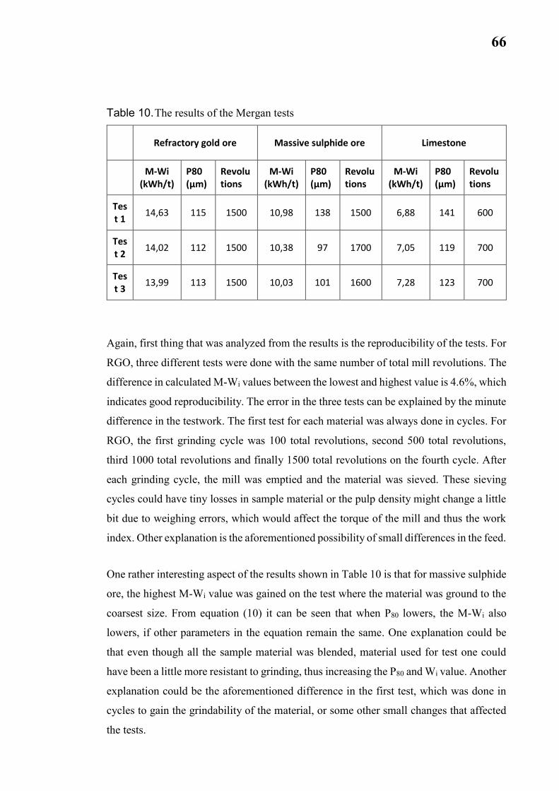
66
Table 10. The results of the Mergan tests
Refractory gold ore Massive sulphide ore Limestone
M-Wi (kWh/t)
P80 (µm)
Revolutions
M-Wi (kWh/t)
P80 (µm)
Revolutions
M-Wi (kWh/t)
P80 (µm)
Revolutions
Test 1
14,63 115 1500 10,98 138 1500 6,88 141 600
Test 2
14,02 112 1500 10,38 97 1700 7,05 119 700
Test 3
13,99 113 1500 10,03 101 1600 7,28 123 700
Again, first thing that was analyzed from the results is the reproducibility of the tests. For
RGO, three different tests were done with the same number of total mill revolutions. The
difference in calculated M-Wi values between the lowest and highest value is 4.6%, which
indicates good reproducibility. The error in the three tests can be explained by the minute
difference in the testwork. The first test for each material was always done in cycles. For
RGO, the first grinding cycle was 100 total revolutions, second 500 total revolutions,
third 1000 total revolutions and finally 1500 total revolutions on the fourth cycle. After
each grinding cycle, the mill was emptied and the material was sieved. These sieving
cycles could have tiny losses in sample material or the pulp density might change a little
bit due to weighing errors, which would affect the torque of the mill and thus the work
index. Other explanation is the aforementioned possibility of small differences in the feed.
One rather interesting aspect of the results shown in Table 10 is that for massive sulphide
ore, the highest M-Wi value was gained on the test where the material was ground to the
coarsest size. From equation (10) it can be seen that when P80 lowers, the M-Wi also
lowers, if other parameters in the equation remain the same. One explanation could be
that even though all the sample material was blended, material used for test one could
have been a little more resistant to grinding, thus increasing the P80 and Wi value. Another
explanation could be the aforementioned difference in the first test, which was done in
cycles to gain the grindability of the material, or some other small changes that affected
the tests.

67
The prediction method used after particle size analysis for each grinding cycle can be
seen in Figure 30, where 106 µm sieve passing% is plotted against total mill revolutions
in the test.
Figure 30. Refractory gold ore Mergan test 1 particle size analysis after each grinding
cycle used to predict grindability in the Mergan mill.
Figure 30 shows that total number of mill revolutions is directly proportional to the 106
µm passing%. When a trendline is added between the points, it can be seen, that when
ground to this fineness, the grindability of the material acts very much like a line, and this
line can be used to predict the grindability of the material after each grinding cycle. Thus
it can also be said, that the ball mill charge, and thus grindability seems to be at an
optimum conditions in the Mergan mill when material is ground to this fineness, as no
significant decrease or increase between the points can be seen. The same effect could
also be observed with the other 2 sample materials used.

68
6.3 Comparison between Bond tests and Mergan tests
The Mergan test and Bond test are quite different. First of all, the mills are of different
size, however, the size difference between the two is proportionate and quite small. The
Bond test is locked cycle test, and the Mergan is a batch test. The mill rotation speed, as
percentage of the critical mill speed, is different. Also, the Mergan mill, even though
smaller in proportions, uses larger ball charge, both in terms of mass and volume. The
amount of material ground in the mills is also vastly different. The Mergan test is done
wet, and Bond test is done dry. In Bond test the P80 is calculated for the sieve under-size,
meanwhile in the Mergan test the P80 value is calculated for the whole test material batch.
It should be noted that both the Bond mill and Mergan mill have been tested extensively
by their creators to find the optimum operating conditions for the mill, so one could
assume that the most notable difference between the two is the fact that that Bond test is
done dry, and the Mergan test is done wet. It should be noted that since the Mergan test
is done in wet conditions, sieving proved to be a lot more flexible with the Mergan
method, and as such, the Mergan method could be a lot more usable when ground to finer
sizes than what can be analyzed with dry sieving.
Table 11 shows the comparison of the three M-Wi values acquired against the average Wi
acquired from the Bond tests when 106 µm sieve was used. The Bond test average is used
because of the fact that the Bond test results have a small error margin, and based on only
three Bond test results it would be safe to assume that the average of those three tests is
the closest to the real Bond work index value. The material in this comparison is the
refractory gold ore.
Table 11. Comparison of the Wi values and M-Wi values for the refractory gold ore.
Wi (kWh/t) Sieve opening (µm) M-Wi (kWh/t) P80 (µm) Difference (%)
Test 1 19,29 106 14,63 115 31,85
Test 2 19,29 106 14,02 112 37,59
Test 3 19,29 106 13,99 113 37,88

69
There is some sort of correlation between the two work indices. The correlation
coefficient value 1.3 from chapter 4.4 is not too far off, but still doesn’t seem very
satisfactory. Table 12 shows the results of the rest of the materials, and comparison is
done to the Bond test where sieve opening is closest to the P80 value gained from the
Mergan tests.
Table 12. Comparison of the Wi values and M-Wi values
Wi (kWh/t)
Sieve opening (µm)
M-Wi (kWh/t)
P80 (µm)
Difference (%)
Refractory gold ore
Test 1
19,29 106 14,63 115 31,85
Test 2
19,29 106 14,02 112 37,59
Test 3
19,29 106 13,99 113 37,88
Massive sulphide ore
Test 1
13,99 150 10,98 138 27,41
Test 2
14,68 106 10,38 97 41,43
Test 3
14,68 106 10,03 101 46,36
Limestone
Test 1
9,21 150 6,88 141 33,87
Test 2
10,21 106 7,05 119 44,82
Test 3
10,21 106 7,28 123 40,25
From Table 12 it is even more visible that there is some sort of correlation between the
two tests, but can’t be explained by a single correlation coefficient. However, when the
two Work indices are plotted against each other, as is done in Figure 31, a more
satisfactory model can be found.
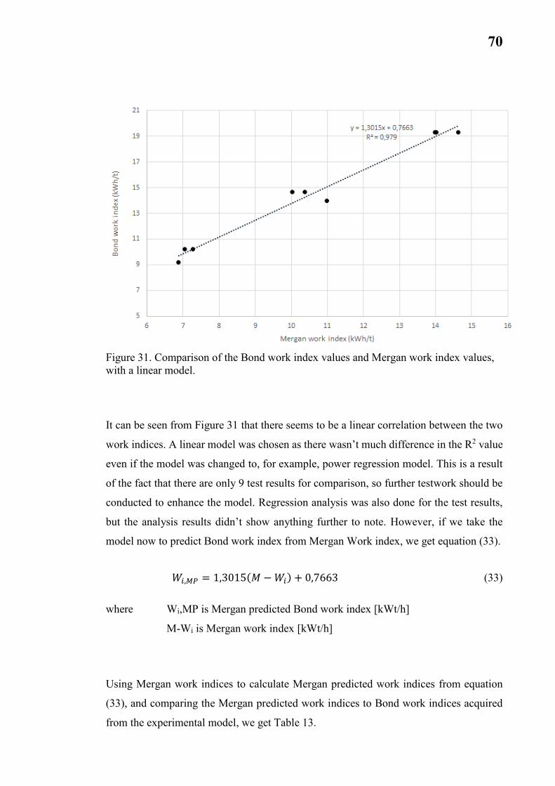
70
Figure 31. Comparison of the Bond work index values and Mergan work index values,
with a linear model.
It can be seen from Figure 31 that there seems to be a linear correlation between the two
work indices. A linear model was chosen as there wasn’t much difference in the R2 value
even if the model was changed to, for example, power regression model. This is a result
of the fact that there are only 9 test results for comparison, so further testwork should be
conducted to enhance the model. Regression analysis was also done for the test results,
but the analysis results didn’t show anything further to note. However, if we take the
model now to predict Bond work index from Mergan Work index, we get equation (33).
𝑊𝑖,𝑀𝑃 = 1,3015(𝑀 − 𝑊𝑖) + 0,7663 (33)
where Wi,MP is Mergan predicted Bond work index [kWt/h]
M-Wi is Mergan work index [kWt/h]
Using Mergan work indices to calculate Mergan predicted work indices from equation
(33), and comparing the Mergan predicted work indices to Bond work indices acquired
from the experimental model, we get Table 13.

71
Table 13. Comparison of Mergan predicted work indices and Bond work indices.
M-Wi (kWh/t) Wi (kWh/t) Wi,MP (kWh/t) Error (%)
Refractory gold ore
Test 1 14,63 19,29 19,81 -2,61
Test 2 14,02 19,29 19,01 1,46
Test 3 13,99 19,29 18,97 1,66
Massive sulphide ore
Test 1 10,98 13,99 15,06 -7,08
Test 2 10,38 14,68 14,28 2,83
Test 3 10,03 14,68 13,82 6,22
Limestone
Test 1 6,88 9,21 9,72 -5,25
Test 2 7,05 10,21 9,94 2,70
Test 3 7,28 10,21 10,24 -0,30
Table 13 shows that for the 9 Mergan tests done during this thesis, the model presented
in equation (33) can predict the Bond work index with a minimum error of 0.30%, and a
maximum of 7.08%, with an average error of 3.35%. The presented experimental model
shows good promise, if it can be believed, that the Mergan mill can indeed be used to
predict the Bond work index for the material. The Work indices are further compared in
Figure 32, where Mergan predicted work indices are plotted against the Bond work
indices from testwork.

72
Figure 32. Comparison of Mergan predicted work indices and Bond work indices.
Going back and taking a look at Table 12 raises one question. Can this comparison be
trusted? The P80 values from the Mergan tests aren’t anywhere near the P80 values from
the Bond tests. Comparison like this can be considered faulty, because the materials aren’t
ground to the same fineness, P80, in both tests. However, Mergan test data can be
normalized mathematically, if a couple of assumptions are made. If we assume that during
the Mergan test, the grindability of the material per mill revolutions is a constant when
going from F80 value to P80 of 75 µm, then the E0 it would take to grind the material to
P80 of 75 µm based on the test data can be calculated, and then the new M-Wi can be
calculated using the new E0 value and assuming that the P80 will be 75 µm. It should be
noted that the Bond test P80 values for RGO were on average 69 µm, but the difference
between 69 and 75 µm is small, and the normalization had to be done to the closest sieve
size possible (75 µm).
This assumption was tested by calculating the mill revolutions it would require for the
massive sulphide ore to be ground to P80 value of 75 µm. After that, one final Mergan test
was conducted, and the results were that M-Wi was 10.46 kWh/t, and the P80 was 77 µm.

73
It was interesting to note that even though the E0 value increased, the decrease in the P80
caused the Mergan work index to stay relatively the same when compared to the other
tests. The minute error of 2 µm caused an error of 1.6% between the Wi values of the one
calculated by normalization and the actual test data. Based on the test, it can be stated that
the grindability for the massive sulphide ore is indeed a constant when ground to P80 of
75 µm. Due to time constraints, the tests couldn’t be conducted to the refractory gold ore
and the limestone to verify this, so the normalization of the data has to be based on the
assumption that the grindability of the limestone and the refractory gold ore also is a
constant when ground to P80 value of 75µm. While this assumption seems reasonable,
since it could not be validated in the testwork, it must be taken with some uncertainty.
The normalized Mergan test data is shown in Table 14. The Mergan predicted Bond work
index are also calculated in Table 14 and compared to the Bond work index averages
when 106 µm sieve closing size was used.
Table 14. Comparison of the Mergan predicted work index values based on data
normalization and Bond work index values from the testwork
Normalized M-Wi (kWh/t)
P80 (µm)
Wi (kWh/t)
Wi,MP (kWh/t)
Error (%)
Refractory gold ore
Test 1
13,68 75 19,29 18,57 3,85
Test 2
13,35 75 19,29 18,15 6,31
Test 3
13,25 75 19,29 18,01 7,11
Massive sulphide
ore
Test 1
9,80 75 14,68 13,52 8,62
Test 2
10,25 75 14,68 14,11 4,06
Test 3
10,26 75 14,68 14,12 3,95
Test 4
10,46 77 14,68 14,38 2,09
Limestone
Test 1
7,01 75 10,21 9,89 3,21
Test 2
6,89 75 10,21 9,74 4,83
Test 3
6,98 75 10,21 9,86 3,60

74
From Table 14 it is visible that based on the normalized test data, the experimental model
seems a little bit worse, with a maximum error of 8.62% and average error of 4.76%. The
comparison this time however is to same product fineness, and as a result the comparison
is be more reliable.
The normalized Mergan work index values are compared to the Bond work index values
in Figure 33 to see if a better model can be based on the normalized Mergan work index
values.
Figure 33. Comparison of the normalized Mergan work index values and the Bond work
index values from the testwork.
We again get a new experimental equation (34) that seems to fit the data better. It is clear
though that the equation is based only on 10 Mergan tests, and their comparison to the
Bond test values, so it is in a sense forced to fit the test data.
𝑊𝑖,𝑀𝑃 = 1,3968(𝑀 − 𝑊𝑖) + 0,483 (34)
Equation (34) is then again used in Table 15, where Mergan predicted Bond work index
values are calculated and compared to the Bond work index values from the testwork. It

75
is visibly clear that the model from equation (34) seems to give better results, and is also
based on a comparison that seems more reliable.
Table 15. Comparison of the normalized Mergan predicted work index values (eq. 34)
and the Bond work index values from the testwork.
Normalized M-Wi (kWh/t) Wi (kWh/t) Wi,MP (kWh/t) Error (%)
13,68 19,29 19,60 1,56
13,35 19,29 19,13 -0,81
13,25 19,29 18,99 -1,59
9,80 14,68 14,17 -3,63
10,25 14,68 14,80 0,81
10,26 14,68 14,82 0,92
10,46 14,68 15,09 2,73
7,01 10,21 10,28 0,65
6,89 10,21 10,11 -0,96
6,98 10,21 10,24 0,27
The model from equation (34) seems to fit the data very well. However, given that the
small sample size that the data presents, and due to the fact that a model that seemed to
fit the data well could be given when a questionable comparison was made to present
equation (33), it is clear that in order to give a better model more test data is required. It
should be also noted that because the data had to be mathematically normalized, small
errors might be present in the normalized Mergan work index values, due to minor
changes in E0 values or differences of a few microns in the P80 value. In my opinion, to
validate this method, up to tens or even hundreds of Mergan tests should be conducted
and compared to Bond work index values, using different materials. Only then it can be
seen if the model is satisfactory across a scale of different materials, and not only fit to
the low amount of test data.
However, based on all of the test data in this thesis, it is safe to assume that the Mergan
test can be used to predict Bond work index values. Niitti (1970) compared W74 values
of Mergan mill and wet industrial grinding process, where he found that the industrial
process had a W74 value of approximately 1.33 times larger than the Mergan mill (Niitti,

76
1970). The results from the testwork seem to correlate with this data as well. Kurki (2006)
also compared Mergan and Bond tests for two ore samples to their grinding circuits, and
found out that the Mergan work index values were approximately 13% and 30% lower
than the Bond work index values (Kurki, 2006).
It is also clear that one should be very careful when comparing grinding tests in terms of
the fineness ground to. Grinding tests should only be compared when ground to same
fineness value in both tests. This taught the author a very valuable lesson about testwork
comparison.

77
7 CONCLUSIONS
The aim of the thesis was to improve the Mergan method so that it could be used to test
grindability and scaled to Bond work index. Literature review of the thesis gave good
insight on how this could be done, and the results from the tests proved that developing
this method seems indeed possible.
Results from the tests show that the Bond and Mergan tests could be done with good
reproducibility. In doing these tests and when analyzing the results, I gained good
knowledge about conducting research, and very good insight on both of these grindability
tests. Bond test results seem to indicate that even though the Bond work index should be
a material specific constant, grinding material to a different size is not always
homogenous in terms of energy consumption. The Bond test also showed that the material
most resistant to grinding had troubles reaching an equilibrium in terms of product created
per mill revolutions. The Sweco sieving method that was used in 75 µm sieving, while
giving reasonable results, had too much material losses and gave a comparably small P80
value, thus making the results questionable.
Based on mineralogical data, Mohs hardness values for each ore sample was also
approximated. Data from the grindability tests showed that the Mohs hardness values
didn’t correlate with resistance to grinding very well.
The results from the Mergan tests indicate 106 µm sieve passing% has a very good linear
correlation with the total number of mill revolutions, at least when ground to fineness
where P80 is about 106 µm. The Mergan method also proved to be quite fast when
information about the grindability of the ore is already known, and proved to be quite
flexible since wet sieving could be used.
Comparison of the two grindability test showed that there is a correlation between the two
work indices, and regression analysis resulted in the creation of an experimental linear
model, where Mergan work index could be used to predict the Bond work index with
good correlation. However, it was noticed that the Mergan tests weren’t done to the same

78
fineness as the Bond tests, and the Mergan test data had to be mathematically normalized.
Based on the normalization a new comparison was done, and another experimental model
is presented. A conclusion is made that based on the test data, the Mergan method can be
used to predict Bond work index values, but to improve and validate the method, more
testwork is required.

79
8 FUTURE TESTWORK
For future testwork, more tests with Mergan mill should be conducted and compared to
Bond test values to enhance the experimental model, using different ore samples and
different sieve closing sizes. Special attention needs to be paid to the fact that P80 values,
or the fineness the ore sample is ground to, should be as close as possible to each other in
both tests.
Although the mathematical normalization of Mergan work index values can be done like
it was done in this testwork, better way to do it is to slightly overgrind the material in the
Mergan mill, and then do the normalization backwards. This way the normalization is not
based on assumptions, but rather backed up with actual test data.
Also one should be very careful not to mix grinding energy consumption (E0) and work
index values with one another, even though both are expressed as kWh/t, they mean
different things.
In terms of mineralogical information and geometallurgy, a good idea for future testing
would be to test if mineralogical data can be used better to approximate grindability of an
ore.

80
9 REFERENCES
Bbosa, L. S., Govender, I., Mainza, A. N. & Powell, M. S., 2011. Power draw estimation
in experimental tumbling mills using PEPT. Minerals Engineering, Volume 24, pp. 319-
324.
Bond, F. C., 1961a. Crushing and grinding calculations, part 1. British Chemical
Engineering, 6(6), pp. 378-385.
Bond, F. C., 1961b. Crushing and grinding calculations, part 2. British chemical
engineering, 6(8), pp. 543-548.
Burger, B. et al., 2006. Batu Hijau Model for Throughput Forecast, Mining and Milling
Optimisation and Expansion Studies. [Online]
Available at:
http://www.metso.com/miningandconstruction/MaTobox7.nsf/DocsByID/15ADE56886
5ADF2EC2257DB700464EA1/$File/batu-hijau-throughput-forecast.pdf
[Accessed 29 August 2017].
Cleary, P. W. & Morrison, R. D., 2016. Comminution mechanisms, particle shape
evolution and collision energy partitioning in tumbling mills. Minerals Engineering,
Volume 86, pp. 75-95.
Fuerstenau, M. C. & Han, K. N., 2003. Principles of Mineral Processing. Littleton,
Colorado: Society for Mining, Metallurgy, and Exploration, Inc..
Gupta, A. & Yan, D. S., 2006. Mineral Processing Design and Operation: An
Introduction. Amsterdam: Burlington Elsevier Science.
Hukki, R. T., 1964. Mineraalien hienonnus ja rikastus. s.l.:Hki: Teknillisten tieteiden
akatemia.

81
Karra, R. C., Subodh, N. H. & Ashwin, J. B., 2016. Prediction of Bond's work index from
field measurable rock properties. International Journal of Mineral Processing, Volume
157, pp. 134-144.
Kurki, P., 2006. Jauhautuvuuden määritys panos-jauhatuskokeilla. s.l.:Helsingin
teknillinen korkeakoulu.
Lamberg, P., 2011. Particles - the bridge between geology and metallurgy. Luleå,
Sweden, Conference in mineral engineering.
Lynch, A. J., 2015. Comminution handbook. Carlton, Victoria: Australian Institute of
Mining and Metallurgy.
Magdalinović, N., 1989. A Procedure for Rapid Determination of the Bond Work Index.
International Journal of Mineral Processing, 27(1-2), pp. 125-132.
Morrell, S., 2004. An alternative energy-size relationship to that proposed by Bond for
the design and optimisation of grinding circuits. International Journal of Mineral
Processing, 74(1-4), pp. 133-141.
Mwanga, A., Rosenkranz, J. & Lamberg, P., 2017. Development and experimental
validation of the Geometallurgical Comminution Test (GCT). Minerals Engineering,
Volume 108, pp. 109-114.
Mörsky, P., Klementti, M. & Knuutinen, T., 1995. A Comparison of High Pressure Roller
Mill and Conventional Grinding. San Francisco, Society for Mining, Metallurgy, and
Exploration, Inc..
Nematollahi, H., 1994. New size laboratory ball mill for Bond work index determination.
Mining Engineering, 46(4), pp. 352-353.
Niitti, T., 1970. Rapid evaluation of grindability by a simple batch test. Praha,
Proceedings of IX IMPC.

82
Norazirah, A., Fuad, S. & Hazizan, M., 2016. The Effect of Size and Shape on Breakage
Characteristics of Mineral. Procedia Chemistry, Volume 19, pp. 702-708.
Rose, H. E. & Sullivan, R., 1958. A Treatise on the internal mechanics of ball, tube and
rod mills. London: s.n.
Starkey, J. & Scinto, P., 2010. SAG Mill Grinding Design Versus Geometallurgy - Getting
It Right For Competent Ores. [Online]
Available at: http://www.sagdesign.com/Papers_for_Website/Brisbane%20Paper.pdf
[Accessed 28 August 2017].
Steiner, H. J., 1996. Characterization of laboratory-scale tumbling mills. International
Journal of Mineral Processing, Volume 44-45, pp. 373-382.
Tüzün, M. A., 2001. Wet bond mill test. Minerals Engineering, 14(3), pp. 369-373.
Walters, S. G., 2008. An overview of new integrated geometallurgical research.
Australian Institute of Mining and Metallurgy Publication Series, pp. 79-82.
Wills, B. A. & Finch, J., 2015. Wills Mineral Processing Technology. 8th ed. Burlington:
Butterworth-Heinemann.
Zhitie, Z., 1995. Catastrophe Theory and Dissipative Structure in Mineral Comminution.
San Francisco, Society for Mining, Metallurgy, and Exploration, Inc..

83
10 APPENDICES
Appendix 1-5. RGO Bond tests
Appendix 6-10. MSO Bond tests
Appendix 11-15. Limestone Bond tests
Appendix 16. RGO Mergan test data
Appendix 17-18. MSO Mergan test data
Appendix 19. Limestone Mergan test data
Appendix 20. RGO and MSO XRD results
Appendix 21. Limestone XRD results
Appendix 22. Mineralogy and hardness calculations
Appendix 23. RGO optical microscope pictures
Appendix 24. MSO optical microscope pictures
Appendix 25. Limestone optical microscope pictures

84
Appendix 1. RGO Bond test, 106µm
RGO
Koe: 19.4.2017
1283,3
9,8
366,7
106
100
Karkeaa Hienoa Hävikki Täydennys Jossa hie- Tuotettu Hienoa/ Tuotettava Tarvittavat Kierto- Hävikki,
Kierros g g g g noa,g hienoa,g myllyn kier hienoa,g seuraavat kuorma,% %:a syöt-
ros,g kierrokset teestä Suunta
1 1091,9 188,7 2,7 191,4 18,7 66,2 0,662 348,0 526 570 0,2
2 917,1 362 4,2 366,2 35,7 347,5 0,661 330,9 501 250 0,3
3 869 410,4 3,9 414,3 40,4 378,6 0,756 326,2 431 210 0,3
4 857,2 422,9 3,2 426,1 41,6 385,7 0,894 325,1 364 201 0,2
5 937,5 342,2 3,6 345,8 33,7 304,2 0,837 332,9 398 271 0,3
6 919,4 356 7,9 363,9 35,5 330,2 0,830 331,2 399 253 0,6
7 877,9 402,8 2,6 405,4 39,5 369,9 0,927 327,1 353 217 0,2
8 937,9 342,8 2,6 345,4 33,7 305,9 0,867 333,0 384 272 0,2
9 928,8 344,4 10,1 354,5 34,6 320,8 0,835 332,1 398 262 0,8
10 897,4 383,8 2,1 385,9 37,6 351,3 0,883 329,0 372 233 0,2
11 938,8 341,4 3,1 344,5 33,6 306,9 0,824 333,0 404 273 0,2
12
13
14
15
Gbp= 0,848 g/ kierros Syöte d80 = 2304 µm
Keskihaj. 0,026 * VALMIS * Tuote d80 = 71 µm
Keskihaj. 3,0 % keskiarvosta Wi= 19,74 kWh/t
Gbp min 0,8240
Gbp max 0,8835
max/min 7,2208
Syöte: Seulalle jäi, Kumulat. Läpäisy,% Tuote: Seulalle jäi Kumulat. Raeluokan Läpäisy, Raeluokan
Raekoko,µm g summa,g Syöte Raekoko,µm g massa,g massa,g Tuote osuus,%
3350 0 100 106 0 0,0 0,0 100,0 0,0
2360 109,2 17,90 17,90 82,10 90 1,1 1,1 1,1 94,7 5,3
1700 151,7 24,87 42,78 57,22 75 2,5 3,6 2,5 82,7 12,0
1180 94,8 15,54 58,32 41,68 53 3,5 7,1 3,5 65,9 16,8
850 50 8,20 66,52 33,48 45 1,2 8,3 1,2 60,1 5,8
600 42,1 6,90 73,42 26,58 -45 12,5 20,8 12,5 0,0 60,1
425 31,2 5,12 78,54 21,46 20,8 0,0 0,0
300 26,7 4,38 82,92 17,08 Yhteensä 20,8 100,0
212 19 3,12 86,03 13,97
150 16,6 2,72 88,75 11,25
106 9,1 1,49 90,24 9,76
75 11,1 1,82 92,06 7,94 Index (S) x y X80, µm
Pan 48,4 7,94 100,00 1 75 82,7 71
609,9 100,00 2 53 65,9
Huom! alkupunnituksesta kamaa +0,5g!!!!!
Index (S) x y X80, µm
1 2360 82,1 2304
2 1700 57,2
Wi 19,740
Katkaisuseula, µm
Aloituskierrokset
Jauhettava materiaali:
Jauhatuspanos, g
Hienoainesta, %
Kiertokuorma, g
0
10
20
30
40
50
60
70
80
90
100
10 100 1000 10000
Lä
pä
isy
, %
Raekoko (µm)
RGO Syöte
Tuote
0,0000,1000,2000,3000,4000,5000,6000,7000,8000,9001,000
0 2 4 6 8 10 12 14 16

85
Appendix 2. RGO Bond test, 106µm
RGO
Koe: 3.5.2017
1283,3
9,8
366,7
106
100
Karkeaa Hienoa Hävikki Täydennys Jossa hie- Tuotettu Hienoa/ Tuotettava Tarvittavat Kierto- Hävikki,
Kierros g g g g noa,g hienoa,g myllyn kier hienoa,g seuraavat kuorma,% %:a syöt-
ros,g kierrokset teestä Suunta
1 1089,8 190,6 2,9 193,5 18,9 68,3 0,683 347,8 509 563 0,2
2 910 371 2,3 373,3 36,4 354,4 0,696 330,2 474 244 0,2
3 904,9 375,9 2,5 378,4 36,9 342,0 0,721 329,7 457 239 0,2
4 860,9 420,5 1,9 422,4 41,2 385,5 0,843 325,4 386 204 0,1
5 931,1 349,5 2,7 352,2 34,4 311,0 0,805 332,3 413 264 0,2
6 890,8 388,9 3,6 392,5 38,3 358,1 0,868 328,4 378 227 0,3
7 936 343 4,3 347,3 33,9 309,0 0,817 332,8 407 270 0,3
8 894,7 384,9 3,7 388,6 37,9 354,7 0,871 328,7 378 230 0,3
9
10
11
12
13
14
15
Gbp= 0,852 g/ kierros Syöte d80 = 2304 µm
Keskihaj. 0,025 * VALMIS * Tuote d80 = 69 µm
Keskihaj. 2,9 % keskiarvosta Wi= 19,32 kWh/t
Gbp min 0,8167
Gbp max 0,8706
max/min 6,5939
Syöte: Seulalle jäi, Kumulat. Läpäisy,% Tuote: Seulalle jäi Kumulat. Raeluokan Läpäisy, Raeluokan
Raekoko,µm g summa,g Syöte Raekoko,µm g massa,g massa,g Tuote osuus,%
3350 100 106 0 0,0 0,0 100,0 0,0
2360 109,2 17,90 17,90 82,10 90 0,7 0,7 0,7 96,8 3,2
1700 151,7 24,87 42,78 57,22 75 2,8 3,5 2,8 84,2 12,6
1180 94,8 15,54 58,32 41,68 53 3,7 7,2 3,7 67,6 16,7
850 50 8,20 66,52 33,48 45 1,5 8,7 1,5 60,8 6,8
600 42,1 6,90 73,42 26,58 -45 13,5 22,2 13,5 0,0 60,8
425 31,2 5,12 78,54 21,46 22,2 0,0 0,0
300 26,7 4,38 82,92 17,08 Yhteensä 22,2 100,0
212 19 3,12 86,03 13,97
150 16,6 2,72 88,75 11,25
106 9,1 1,49 90,24 9,76
75 11,1 1,82 92,06 7,94 Index (S) x y X80, µm
Pan 48,4 7,94 100,00 1 75 84,2 69
609,9 100,00 2 53 67,6
Huom! alkupunnituksesta kamaa +0,5g!!!!!
Index (S) x y X80, µm
1 2360 82,1 2304
2 1700 57,2
Wi 19,319
Katkaisuseula, µm
Aloituskierrokset
Jauhettava materiaali:
Jauhatuspanos, g
Hienoainesta, %
Kiertokuorma, g
0
10
20
30
40
50
60
70
80
90
100
10 100 1000 10000
Läpäisy,
%
Raekoko (µm)
RGO Syöte
Tuote
0,0000,1000,2000,3000,4000,5000,6000,7000,8000,9001,000
0 2 4 6 8 10 12 14 16

86
Appendix 3. RGO Bond test, 106µm
RGO
Koe: 26.7.2017
1283,3
9,8
366,7
106
100
Karkeaa Hienoa Hävikki Täydennys Jossa hie- Tuotettu Hienoa/ Tuotettava Tarvittavat Kierto- Hävikki,
Kierros g g g g noa,g hienoa,g myllyn kier hienoa,g seuraavat kuorma,% %:a syöt-
ros,g kierrokset teestä Suunta
1 1093,1 188,2 2,0 190,2 18,6 65,0 0,650 348,1 535 575 0,2
2 936,2 344,3 2,8 347,1 33,9 328,5 0,614 332,8 542 270 0,2
3 855,5 424,3 3,5 427,8 41,7 393,9 0,726 324,9 447 200 0,3
4 894,5 385,6 3,2 388,8 37,9 347,1 0,776 328,7 424 230 0,2
5 855,8 424,1 3,4 427,5 41,7 389,6 0,919 325,0 353 200 0,3
6 939,5 341,2 2,6 343,8 33,5 302,1 0,855 333,1 390 273 0,2
7 936,5 344,6 2,2 346,8 33,8 313,3 0,804 332,8 414 270 0,2
8 885 395,3 3,0 398,3 38,9 364,5 0,880 327,8 372 222 0,2
9 924,2 353,1 6 359,1 35,0 320,2 0,860 331,6 386 257 0,5
10 928 351,5 3,8 355,3 34,7 320,3 0,830 332,0 400 261 0,3
11
12
13
14
15
Gbp= 0,857 g/ kierros Syöte d80 = 2304 µm
Keskihaj. 0,020 * VALMIS * Tuote d80 = 67 µm
Keskihaj. 2,4 % keskiarvosta Wi= 18,81 kWh/t
Gbp min 0,8304
Gbp max 0,8801
max/min 5,9896
Syöte: Seulalle jäi, Kumulat. Läpäisy,% Tuote: Seulalle jäi Kumulat. Raeluokan Läpäisy, Raeluokan
Raekoko,µm g summa,g Syöte Raekoko,µm g massa,g massa,g Tuote osuus,%
3350 0 100 106 0 0,0 0,0 100,0 0,0
2360 109,2 17,90 17,90 82,10 90 0,6 0,6 0,6 97,3 2,7
1700 151,7 24,87 42,78 57,22 75 2,4 3,0 2,4 86,4 10,9
1180 94,8 15,54 58,32 41,68 53 3,9 6,9 3,9 68,8 17,6
850 50 8,20 66,52 33,48 45 1,4 8,3 1,4 62,4 6,3
600 42,1 6,90 73,42 26,58 -45 13,8 22,1 13,8 0,0 62,4
425 31,2 5,12 78,54 21,46 22,1 0,0 0,0
300 26,7 4,38 82,92 17,08 Yhteensä 22,1 100,0
212 19 3,12 86,03 13,97
150 16,6 2,72 88,75 11,25
106 9,1 1,49 90,24 9,76
75 11,1 1,82 92,06 7,94 Index (S) x y X80, µm
Pan 48,4 7,94 100,00 1 75 86,42533937 67
609,9 100,00 2 53 68,77828054
Huom! alkupunnituksesta kamaa +0,5g!!!!!
Index (S) x y X80, µm
1 2360 82,1 2304
2 1700 57,2
Wi 18,815
Katkaisuseula, µm
Aloituskierrokset
Jauhettava materiaali:
Jauhatuspanos, g
Hienoainesta, %
Kiertokuorma, g
0
10
20
30
40
50
60
70
80
90
100
10 100 1000 10000
Lä
pä
isy
, %
Raekoko (µm)
RGO Syöte
Tuote
0,0000,1000,2000,3000,4000,5000,6000,7000,8000,9001,000
0 2 4 6 8 10 12 14 16

87
Appendix 4. RGO Bond test, 150µm
RGO
Koe: 28.4.2017
1283,3
11,2
366,7
150
100
Karkeaa Hienoa Hävikki Täydennys Jossa hie- Tuotettu Hienoa/ Tuotettava Tarvittavat Kierto- Hävikki,
Kierros g g g g noa,g hienoa,g myllyn kier hienoa,g seuraavat kuorma,% %:a syöt-
ros,g kierrokset teestä Suunta
1 1045,2 235,3 2,8 238,1 26,8 93,8 0,938 339,9 363 439 0,2
2 947,5 333,7 2,1 335,8 37,8 309,0 0,852 328,9 386 282 0,2
3 897,8 382,2 3,3 385,5 43,4 347,7 0,901 323,3 359 233 0,3
4 893,5 388,3 1,5 389,8 43,8 346,4 0,966 322,8 334 229 0,1
5 912,8 369,1 1,4 370,5 41,7 326,7 0,977 325,0 333 246 0,1
6 913,9 366,6 2,8 369,4 41,5 327,7 0,986 325,1 330 247 0,2
7 914,9 366 2,4 368,4 41,4 326,9 0,991 325,2 328 248 0,2
8 920,1 360 3,2 363,2 40,9 321,8 0,980 325,8 332 253 0,2
9
10
11
12
13
14
15
Gbp= 0,986 g/ kierros Syöte d80 = 2304 µm
Keskihaj. 0,004 * VALMIS * Tuote d80 = 97 µm
Keskihaj. 0,4 % keskiarvosta Wi= 19,39 kWh/t
Gbp min 0,9803
Gbp max 0,9908
max/min 1,0744
Syöte: Seulalle jäi, Kumulat. Läpäisy,% Tuote: Seulalle jäi Kumulat. Raeluokan Läpäisy, Raeluokan
Raekoko,µm g summa,g Syöte Raekoko,µm g massa,g massa,g Tuote osuus,%
3350 100 125 1,7 1,7 1,7 92,1 7,9
2360 109,2 17,90 17,90 82,10 106 1,4 3,1 1,4 85,5 6,5
1700 151,7 24,87 42,78 57,22 90 2 5,1 2,0 76,2 9,3
1180 94,8 15,54 58,32 41,68 75 1,9 7,0 1,9 67,3 8,9
850 50 8,20 66,52 33,48 53 3,1 10,1 3,1 52,8 14,5
600 42,1 6,90 73,42 26,58 45 0,6 10,7 0,6 50,0 2,8
425 31,2 5,12 78,54 21,46 -45 10,7 21,4 10,7 50,0
300 26,7 4,38 82,92 17,08 Yhteensä 21,4 100,0
212 19 3,12 86,03 13,97
150 16,6 2,72 88,75 11,25
106 9,1 1,49 90,24 9,76
75 11,1 1,82 92,06 7,94 Index (S) x y X80, µm
Pan 48,4 7,94 100,00 1 106 85,5 97
609,9 100,00 2 90 76,2
Huom! alkupunnituksesta kamaa +0,5g!!!!!
Index (S) x y X80, µm
1 2360 82,1 2304
2 1700 57,2
Wi 19,389
Katkaisuseula, µm
Aloituskierrokset
Jauhettava materiaali:
Jauhatuspanos, g
Hienoainesta, %
Kiertokuorma, g
0
10
20
30
40
50
60
70
80
90
100
10 100 1000 10000
Läpäisy,
%
Raekoko (µm)
RGO Syöte
Tuote
0,000
0,200
0,400
0,600
0,800
1,000
0 2 4 6 8 10 12 14 16

88
Appendix 5. RGO Bond test, 75 µm
RGO
Koe: 20.7.2017
1283,3
7,9
366,7
75
100
Karkeaa Hienoa Hävikki Täydennys Jossa hie- Tuotettu Hienoa/ Tuotettava Tarvittavat Kierto- Hävikki,
Kierros g g g g noa,g hienoa,g myllyn kier hienoa,g seuraavat kuorma,% %:a syöt-
ros,g kierrokset teestä Suunta
1 1134,5 93,3 55,5 148,8 11,8 47,0 0,470 354,8 756 762 4,3
2 914,7 359,6 9,0 368,6 29,3 356,8 0,472 337,4 715 248 0,7
3 945 327,1 11,2 338,3 26,8 309,0 0,432 339,8 786 279 0,9
4 955,9 315,7 11,7 327,4 26,0 300,6 0,383 340,7 891 292 0,9
5 790,6 462,5 30,2 492,7 39,1 466,7 0,524 327,6 625 160 2,4
6 920,8 353,3 9,2 362,5 28,8 323,4 0,517 337,9 653 254 0,7
7 898,1 378,1 7,1 385,2 30,6 356,4 0,546 336,1 616 233 0,6
8
9
10
11
12
13
14
15
Gbp= 0,529 g/ kierros Syöte d80 = 2304 µm
Keskihaj. 0,012 * VALMIS * Tuote d80 = 33 µm
Keskihaj. 2,3 % keskiarvosta Wi= 20,02 kWh/t
Gbp min 0,5174
Gbp max 0,5458
max/min 5,4878
Syöte: Seulalle jäi, Kumulat. Läpäisy,% Tuote: Seulalle jäi Kumulat. Raeluokan Läpäisy, Raeluokan
Raekoko,µm g summa,g Syöte Raekoko,µm g massa,g massa,g Tuote osuus,%
3350 0 100 0,0 0,0 100,0 0,0
2360 109,2 17,90 17,90 82,10 0,0 0,0 100,0 0,0
1700 151,7 24,87 42,78 57,22 75 0 0,0 0,0 100,0 0,0
1180 94,8 15,54 58,32 41,68 45 0,7 0,7 0,7 96,1 3,9
850 50 8,20 66,52 33,48 38 0,9 1,6 0,9 91,0 5,1
600 42,1 6,90 73,42 26,58 20 7,1 8,7 7,1 51,1 39,9
425 31,2 5,12 78,54 21,46 -20 9,1 17,8 9,1 51,1
300 26,7 4,38 82,92 17,08 Yhteensä 17,8 100,0
212 19 3,12 86,03 13,97
150 16,6 2,72 88,75 11,25
106 9,1 1,49 90,24 9,76
75 11,1 1,82 92,06 7,94 Index (S) x y X80, µm
Pan 48,4 7,94 100,00 1 38 91,01123596 33
609,9 100,00 2 20 51,12359551
Huom! alkupunnituksesta kamaa +0,5g!!!!!
Index (S) x y X80, µm
1 2360 82,1 2304
2 1700 57,2
Wi 20,015
Katkaisuseula, µm
Aloituskierrokset
Jauhettava materiaali:
Jauhatuspanos, g
Hienoainesta, %
Kiertokuorma, g
0
10
20
30
40
50
60
70
80
90
100
10 100 1000 10000
Läpäisy,
%
Raekoko (µm)
RGO Syöte
Tuote
0,0000,1000,2000,3000,4000,5000,6000,7000,8000,9001,000
0 2 4 6 8 10 12 14 16

89
Appendix 6. MSO Bond test, 106 µm
MSO
Koe: 19.5.2017
1704,2
10,7
486,9
106
100
Karkeaa Hienoa Hävikki Täydennys Jossa hie- Tuotettu Hienoa/ Tuotettava Tarvittavat Kierto- Hävikki,
Kierros g g g g noa,g hienoa,g myllyn kier hienoa,g seuraavat kuorma,% %:a syöt-
ros,g kierrokset teestä Suunta
1 1382 318,6 3,6 322,2 34,5 139,6 1,396 452,4 324 429 0,2
2 1276,1 425,7 2,4 428,1 45,9 393,6 1,214 441,0 363 298 0,1
3 1208,9 490,5 4,8 495,3 53,1 449,4 1,237 433,8 351 244 0,3
4 1221 480,5 2,7 483,2 51,8 430,1 1,227 435,1 355 253 0,2
5 1208,4 492 3,8 495,8 53,1 444,0 1,252 433,8 347 244 0,2
6 1205,2 496,1 2,9 499 53,5 445,9 1,287 433,4 337 242 0,2
7 1220,7 479 4,5 483,5 51,8 430,0 1,276 435,1 341 252 0,3
8
9
10
11
12
13
14
15
Gbp= 1,272 g/ kierros Syöte d80 = 2244 µm
Keskihaj. 0,015 * VALMIS * Tuote d80 = 75 µm
Keskihaj. 1,2 % keskiarvosta Wi= 14,62 kWh/t
Gbp min 1,2517
Gbp max 1,2866
max/min 2,7861
Syöte: Seulalle jäi, Kumulat. Läpäisy,% Tuote: Seulalle jäi Kumulat. Raeluokan Läpäisy, Raeluokan
Raekoko,µm g summa,g Syöte Raekoko,µm g massa,g massa,g Tuote osuus,%
3350 0 100 106 0 0,0 0,0 100,0 0,0
2360 143,80 15,74 15,74 84,26 90 0,9 0,9 0,9 94,2 5,8
1700 220,80 24,17 39,91 60,09 75 2,2 3,1 2,2 80,0 14,2
1180 166,30 18,20 58,12 41,88 53 2,9 6,0 2,9 61,3 18,7
850 86,40 9,46 67,58 32,42 45 1,3 7,3 1,3 52,9 8,4
600 61,50 6,73 74,31 25,69 -45 8,2 15,5 8,2 0,0 52,9
425 42,10 4,61 78,92 21,08 15,5 0,0 0,0
300 33,90 3,71 82,63 17,37 Yhteensä 15,5 100,0
212 25,20 2,76 85,39 14,61
150 24,00 2,63 88,01 11,99
106 11,60 1,27 89,28 10,72
75 20,20 2,21 91,49 8,51 Index (S) x y X80, µm
Pan 77,70 8,51 100,00 1 75 80 75
913,5 100,00 2
Huom! alkupunnituksesta kamaa +0,5g!!!!!
Index (S) x y X80, µm
1 2360 84,3 2244
2 1700 60,1
Wi 14,619
Katkaisuseula, µm
Aloituskierrokset
Jauhettava materiaali:
Jauhatuspanos, g
Hienoainesta, %
Kiertokuorma, g
0
10
20
30
40
50
60
70
80
90
100
10 100 1000 10000
Lä
pä
isy
, %
Raekoko (µm)
MSO Syöte
Tuote
0,000
0,200
0,400
0,600
0,800
1,000
1,200
1,400
0 2 4 6 8 10 12 14 16

90
Appendix 7. MSO Bond test, 106 µm
MSO
Koe: 24.5.2017
1704,2
10,7
486,9
106
100
Karkeaa Hienoa Hävikki Täydennys Jossa hie- Tuotettu Hienoa/ Tuotettava Tarvittavat Kierto- Hävikki,
Kierros g g g g noa,g hienoa,g myllyn kier hienoa,g seuraavat kuorma,% %:a syöt-
ros,g kierrokset teestä Suunta
1 1385,6 314,1 4,5 318,6 34,1 136,0 1,360 452,8 333 435 0,3
2 1261,7 437,7 4,8 442,5 47,4 408,4 1,226 439,5 358 285 0,3
3 1232,2 468,3 3,7 472 50,6 424,6 1,185 436,3 368 261 0,2
4 1211,2 490 3,0 493 52,8 442,4 1,201 434,1 361 246 0,2
5 1204,1 496,9 3,2 500,1 53,6 447,3 1,238 433,3 350 241 0,2
6 1209,4 491,6 3,2 494,8 53,0 441,2 1,260 433,9 344 244 0,2
7 1197,9 502,8 3,5 506,3 54,3 453,3 1,316 432,7 329 237 0,2
8 1228,6 471,8 3,8 475,6 51,0 421,3 1,282 435,9 340 258 0,2
9
10
11
12
13
14
15
Gbp= 1,286 g/ kierros Syöte d80 = 2244 µm
Keskihaj. 0,023 * VALMIS * Tuote d80 = 76 µm
Keskihaj. 1,8 % keskiarvosta Wi= 14,58 kWh/t
Gbp min 1,2602
Gbp max 1,3165
max/min 4,4679
Syöte: Seulalle jäi, Kumulat. Läpäisy,% Tuote: Seulalle jäi Kumulat. Raeluokan Läpäisy, Raeluokan
Raekoko,µm g summa,g Syöte Raekoko,µm g massa,g massa,g Tuote osuus,%
3350 0 100 106 0,0 0,0 100,0 0,0
2360 143,8 15,74 15,74 84,26 90 1 1,0 1,0 93,3 6,7
1700 220,8 24,17 39,91 60,09 75 2,1 3,1 2,1 79,2 14,1
1180 166,3 18,20 58,12 41,88 53 2,7 5,8 2,7 61,1 18,1
850 86,4 9,46 67,58 32,42 45 1,2 7,0 1,2 53,0 8,1
600 61,5 6,73 74,31 25,69 -45 7,9 14,9 7,9 0,0 53,0
425 42,1 4,61 78,92 21,08 14,9 0,0 0,0
300 33,9 3,71 82,63 17,37 Yhteensä 14,9 100,0
212 25,2 2,76 85,39 14,61
150 24 2,63 88,01 11,99
106 11,6 1,27 89,28 10,72
75 20,2 2,21 91,49 8,51 Index (S) x y X80, µm
Pan 77,7 8,51 100,00 1 90 93,3 76
913,5 100,00 2 75 79,2
Huom! alkupunnituksesta kamaa +0,5g!!!!!
Index (S) x y X80, µm
1 2360 84,26 2244
2 1700 60,09
Wi 14,583
Katkaisuseula, µm
Aloituskierrokset
Jauhettava materiaali:
Jauhatuspanos, g
Hienoainesta, %
Kiertokuorma, g
0
10
20
30
40
50
60
70
80
90
100
10 100 1000 10000
Läpäisy,
%
Raekoko (µm)
MSO Syöte
Tuote
0,000
0,200
0,400
0,600
0,800
1,000
1,200
1,400
1,600
0 2 4 6 8 10 12 14 16

91
Appendix 8. MSO Bond test, 106 µm
MSO
Koe: 2.8.2017
1704,2
10,7
486,9
106
100
Karkeaa Hienoa Hävikki Täydennys Jossa hie- Tuotettu Hienoa/ Tuotettava Tarvittavat Kierto- Hävikki,
Kierros g g g g noa,g hienoa,g myllyn kier hienoa,g seuraavat kuorma,% %:a syöt-
ros,g kierrokset teestä Suunta
1 1397,4 303,6 3,2 306,8 32,9 124,2 1,242 454,0 366 455 0,2
2 1254,1 446,6 3,5 450,1 48,2 417,2 1,141 438,7 384 279 0,2
3 1214,2 488,6 1,4 490 52,5 441,8 1,149 434,4 378 248 0,1
4 1204,3 498 1,9 499,9 53,6 447,4 1,183 433,3 366 241 0,1
5 1198,4 501,8 4,0 505,8 54,2 452,2 1,235 432,7 350 237 0,2
6 1223,7 478,1 2,4 480,5 51,5 426,3 1,217 435,4 358 255 0,1
7
8
9
10
11
12
13
14
15
Gbp= 1,212 g/ kierros Syöte d80 = 2244 µm
Keskihaj. 0,021 * VALMIS * Tuote d80 = 72 µm
Keskihaj. 1,8 % keskiarvosta Wi= 14,83 kWh/t
Gbp min 1,1833
Gbp max 1,2349
max/min 4,3582
Syöte: Seulalle jäi, Kumulat. Läpäisy,% Tuote: Seulalle jäi Kumulat. Raeluokan Läpäisy, Raeluokan
Raekoko,µm g summa,g Syöte Raekoko,µm g massa,g massa,g Tuote osuus,%
3350 0 100 106 0 0,0 0,0 100,0 0,0
2360 143,8 15,74 15,74 84,26 90 0,7 0,7 0,7 95,6 4,4
1700 220,8 24,17 39,91 60,09 75 2,1 2,8 2,1 82,3 13,3
1180 166,3 18,20 58,12 41,88 53 2,6 5,4 2,6 65,8 16,5
850 86,4 9,46 67,58 32,42 45 1,1 6,5 1,1 58,9 7,0
600 61,5 6,73 74,31 25,69 -45 9,3 15,8 9,3 0,0 58,9
425 42,1 4,61 78,92 21,08 15,8 0,0 0,0
300 33,9 3,71 82,63 17,37 Yhteensä 15,8 100,0
212 25,2 2,76 85,39 14,61
150 24 2,63 88,01 11,99
106 11,6 1,27 89,28 10,72
75 20,2 2,21 91,49 8,51 Index (S) x y X80, µm
Pan 77,7 8,51 100,00 1 75 82,27848101 72
913,5 100,00 2 53 65,82278481
Huom! alkupunnituksesta kamaa +0,5g!!!!!
Index (S) x y X80, µm
1 2360 84,3 2244
2 1700 60,1
Wi 14,830
Katkaisuseula, µm
Aloituskierrokset
Jauhettava materiaali:
Jauhatuspanos, g
Hienoainesta, %
Kiertokuorma, g
0
10
20
30
40
50
60
70
80
90
100
10 100 1000 10000
Lä
pä
isy
, %
Raekoko (µm)
MSO Syöte
Tuote
0,000
0,200
0,400
0,600
0,800
1,000
1,200
1,400
1,600
0 2 4 6 8 10 12 14 16

92
Appendix 9. MSO Bond test, 150 µm
MSO
Koe: 22.5.2017
1704,2
12,0
486,9
150
100
Karkeaa Hienoa Hävikki Täydennys Jossa hie- Tuotettu Hienoa/ Tuotettava Tarvittavat Kierto- Hävikki,
Kierros g g g g noa,g hienoa,g myllyn kier hienoa,g seuraavat kuorma,% %:a syöt-
ros,g kierrokset teestä Suunta
1 1320 381,4 2,8 384,2 46,1 179,9 1,799 440,9 245 344 0,2
2 1273,2 427,9 3,1 431 51,7 384,9 1,571 435,3 277 295 0,2
3 1228,7 471,4 4,1 475,5 57,0 423,8 1,530 429,9 281 258 0,2
4 1212,6 488 3,6 491,6 58,9 434,6 1,546 428,0 277 247 0,2
5 1206,5 494,2 3,5 497,7 59,7 438,8 1,585 427,3 269 242 0,2
6 1219,1 481,9 3,2 485,1 58,1 425,4 1,579 428,8 272 251 0,2
7
8
9
10
11
12
13
14
15
Gbp= 1,570 g/ kierros Syöte d80 = 2244 µm
Keskihaj. 0,017 * VALMIS * Tuote d80 = 105 µm
Keskihaj. 1,1 % keskiarvosta Wi= 13,99 kWh/t
Gbp min 1,5465
Gbp max 1,5855
max/min 2,5201
Syöte: Seulalle jäi, Kumulat. Läpäisy,% Tuote: Seulalle jäi Kumulat. Raeluokan Läpäisy, Raeluokan
Raekoko,µm g summa,g Syöte Raekoko,µm g massa,g massa,g Tuote osuus,%
3350 0 100 150 0 0,0 0,0 100,0 0,0
2360 143,80 15,74 15,74 84,26 106 2,8 2,8 2,8 80,7 19,3
1700 220,80 24,17 39,91 60,09 90 1,3 4,1 1,3 71,7 9,0
1180 166,30 18,20 58,12 41,88 75 1,4 5,5 1,4 62,1 9,7
850 86,40 9,46 67,58 32,42 53 1,9 7,4 1,9 49,0 13,1
600 61,50 6,73 74,31 25,69 45 0,8 8,2 0,8 43,4 5,5
425 42,10 4,61 78,92 21,08 -45 6,3 14,5 6,3 43,4
300 33,90 3,71 82,63 17,37 Yhteensä 14,5 100,0
212 25,20 2,76 85,39 14,61
150 24,00 2,63 88,01 11,99
106 11,60 1,27 89,28 10,72
75 20,20 2,21 91,49 8,51 Index (S) x y X80, µm
Pan 77,70 8,51 100,00 1 106 80,7 105
913,5 100,00 2 90 71,7
Huom! alkupunnituksesta kamaa +0,5g!!!!!
Index (S) x y X80, µm
1 2360 84,3 2244
2 1700 60,1
Wi 13,986
Katkaisuseula, µm
Aloituskierrokset
Jauhettava materiaali:
Jauhatuspanos, g
Hienoainesta, %
Kiertokuorma, g
0
10
20
30
40
50
60
70
80
90
100
10 100 1000 10000
Lä
pä
isy
, %
Raekoko (µm)
MSO Syöte
Tuote
0,0000,2000,4000,6000,8001,0001,2001,4001,6001,8002,000
0 2 4 6 8 10 12 14 16

93
Appendix 10. MSO Bond test, 75 µm
MSO
Koe: 24.5.2017
1704,2
8,5
486,9
75
100
Karkeaa Hienoa Hävikki Täydennys Jossa hie- Tuotettu Hienoa/ Tuotettava Tarvittavat Kierto- Hävikki,
Kierros g g g g noa,g hienoa,g myllyn kier hienoa,g seuraavat kuorma,% %:a syöt-
ros,g kierrokset teestä Suunta
1 1410,6 167,4 126,2 293,6 25,0 148,6 1,486 461,9 311 480 7,4
2 1419,7 283,7 0,8 284,5 24,2 259,5 0,835 462,7 554 499 0,0
3 1237,6 457,3 9,3 466,6 39,7 442,4 0,798 447,2 560 265 0,5
4 1214,9 474,7 14,6 489,3 41,6 449,6 0,803 445,3 555 248 0,9
5 1220,2 460,5 23,5 484 41,2 442,4 0,797 445,7 559 252 1,4
6 1211,6 484,1 8,5 492,6 41,9 451,4 0,808 445,0 551 246 0,5
7
8
9
10
11
12
13
14
15
Gbp= 0,803 g/ kierros Syöte d80 = 2244 µm
Keskihaj. 0,004 * VALMIS * Tuote d80 = 39 µm
Keskihaj. 0,5 % keskiarvosta Wi= 15,74 kWh/t
Gbp min 0,7975
Gbp max 0,8076
max/min 1,2755
Syöte: Seulalle jäi, Seulalle jäi, Kumulat. Läpäisy,% Tuote: Seulalle jäi Kumulat. Raeluokan Läpäisy, Raeluokan
Raekoko,µm g % summa,g Syöte Raekoko,µm g massa,g massa,g Tuote osuus,%
3350 0,0 0,0 0 100 0,0 0,0 100,0 0,0
2360 143,8 15,7 15,74 84,3 0,0 0,0 100,0 0,0
1700 220,8 24,2 39,91 60,1 75 0 0,0 0,0 100,0 0,0
1180 166,3 18,2 58,12 41,9 45 1,7 1,7 1,7 88,0 12,0
850 86,4 9,5 67,58 32,4 38 1,4 3,1 1,4 78,2 9,9
600 61,5 6,7 74,31 25,7 -38 11,1 14,2 11,1 0,0 78,2
425 42,1 4,6 78,92 21,1 14,2 0,0 0,0
300 33,9 3,7 82,63 17,4 Yhteensä 14,2 100,0
212 25,2 2,8 85,39 14,6
150 24 2,6 88,01 12,0
106 11,6 1,3 89,28 10,7
75 20,2 2,2 91,49 8,5 Index (S) x y X80, µm
Pan 77,7 8,5 100,00 1 45 88 39
913,5 100,0 2 38 78,2
Huom! alkupunnituksesta kamaa +0,5g!!!!!
Index (S) x y X80, µm
1 2360 84,3 2244
2 1700 60,1
Wi 15,736
Katkaisuseula, µm
Aloituskierrokset
Jauhettava materiaali:
Jauhatuspanos, g
Hienoainesta, %
Kiertokuorma, g
0
10
20
30
40
50
60
70
80
90
100
10 100 1000 10000
Lä
pä
isy
, %
Raekoko (µm)
MSO Syöte
Tuote
0,0000,2000,4000,6000,8001,0001,2001,4001,6001,8002,000
0 2 4 6 8 10 12 14 16

94
Appendix 11. Limestone Bond test, 106 µm
Limestone
Koe: 10.7.2017
1244,1
12,5
355,5
106
100
Karkeaa Hienoa Hävikki Täydennys Jossa hie- Tuotettu Hienoa/ Tuotettava Tarvittavat Kierto- Hävikki,
Kierros g g g g noa,g hienoa,g myllyn kier hienoa,g seuraavat kuorma,% %:a syöt-
ros,g kierrokset teestä Suunta
1 914,1 327,8 2,2 330 41,1 174,9 1,749 314,3 180 277 0,2
2 860,1 380,4 3,6 384 47,9 342,9 1,908 307,6 161 224 0,3
3 868,5 373,1 2,5 375,6 46,8 327,7 2,033 308,6 152 231 0,2
4 883 358,5 2,6 361,1 45,0 314,3 2,070 310,4 150 245 0,2
5 894,8 346,6 2,7 349,3 43,5 304,3 2,029 311,9 154 256 0,2
6 894 348,2 1,9 350,1 43,6 306,6 1,994 311,8 156 255 0,2
7
8
9
10
11
12
13
14
15
Gbp= 2,031 g/ kierros Syöte d80 = 2018 µm
Keskihaj. 0,031 * VALMIS * Tuote d80 = 76 µm
Keskihaj. 1,5 % keskiarvosta Wi= 10,19 kWh/t
Gbp min 1,9943
Gbp max 2,0703
max/min 3,8063
Syöte: Seulalle jäi, Kumulat. Läpäisy,% Tuote: Seulalle jäi Kumulat. Raeluokan Läpäisy, Raeluokan
Raekoko,µm g summa,g Syöte Raekoko,µm g massa,g massa,g Tuote osuus,%
3350 0 100 106 0 0,0 0,0 100,0 0,0
2360 51,1 9,65 9,65 90,35 90 1,3 1,3 1,3 93,8 6,2
1700 105,8 19,98 29,63 70,37 75 3,2 4,5 3,2 78,7 15,2
1180 92,6 17,49 47,12 52,88 53 4,3 8,8 4,3 58,3 20,4
850 58,2 10,99 58,11 41,89 45 1,7 10,5 1,7 50,2 8,1
600 44,1 8,33 66,44 33,56 -45 10,6 21,1 10,6 0,0 50,2
425 32,2 6,08 72,52 27,48 21,1 0,0 0,0
300 27,7 5,23 77,75 22,25 Yhteensä 21,1 100,0
212 20,6 3,89 81,64 18,36
150 19,9 3,76 85,40 14,60
106 11,3 2,13 87,54 12,46
75 15,6 2,95 90,48 9,52 Index (S) x y X80, µm
Pan 50,4 9,52 100,00 1 90 93,8 76
529,5 100,00 2 75 78,7
Huom! alkupunnituksesta kamaa +0,5g!!!!!
Index (S) x y X80, µm
1 2360 90,3 2018
2 1700 70,4
Wi 10,187
Katkaisuseula, µm
Aloituskierrokset
Jauhettava materiaali:
Jauhatuspanos, g
Hienoainesta, %
Kiertokuorma, g
0
10
20
30
40
50
60
70
80
90
100
10 100 1000 10000
Läpäisy,
%
Raekoko (µm)
Limestone Syöte
Tuote
0,0000,2000,4000,6000,8001,0001,2001,4001,6001,8002,0002,200
0 2 4 6 8 10 12 14 16

95
Appendix 12. Limestone Bond test, 106 µm
Limestone
Koe: 13.7.2017
1244,1
12,5
355,5
106
100
Karkeaa Hienoa Hävikki Täydennys Jossa hie- Tuotettu Hienoa/ Tuotettava Tarvittavat Kierto- Hävikki,
Kierros g g g g noa,g hienoa,g myllyn kier hienoa,g seuraavat kuorma,% %:a syöt-
ros,g kierrokset teestä Suunta
1 905,1 336,3 2,7 339 42,3 183,9 1,839 313,2 170 267 0,2
2 874,5 368,1 1,5 369,6 46,1 327,3 1,922 309,4 161 237 0,1
3 880,7 360,5 2,9 363,4 45,3 317,3 1,972 310,2 157 242 0,2
4 871,6 370,3 2,2 372,5 46,4 327,2 2,080 309,0 149 234 0,2
5 897,8 344,1 2,2 346,3 43,2 299,9 2,018 312,3 155 259 0,2
6 893,3 348,2 2,6 350,8 43,7 307,6 1,988 311,7 157 255 0,2
7
8
9
10
11
12
13
14
15
Gbp= 2,029 g/ kierros Syöte d80 = 2018 µm
Keskihaj. 0,038 * VALMIS * Tuote d80 = 76 µm
Keskihaj. 1,9 % keskiarvosta Wi= 10,14 kWh/t
Gbp min 1,9883
Gbp max 2,0800
max/min 4,6138
Syöte: Seulalle jäi, Kumulat. Läpäisy,% Tuote: Seulalle jäi Kumulat. Raeluokan Läpäisy, Raeluokan
Raekoko,µm g summa,g Syöte Raekoko,µm g massa,g massa,g Tuote osuus,%
3350 0 100 106 0 0,0 0,0 100,0 0,0
2360 51,1 9,65 9,65 90,35 90 1,1 1,1 1,1 94,7 5,3
1700 105,8 19,98 29,63 70,37 75 3,2 4,3 3,2 79,3 15,4
1180 92,6 17,49 47,12 52,88 53 4,2 8,5 4,2 59,1 20,2
850 58,2 10,99 58,11 41,89 45 1,8 10,3 1,8 50,5 8,7
600 44,1 8,33 66,44 33,56 -45 10,5 20,8 10,5 0,0 50,5
425 32,2 6,08 72,52 27,48 20,8 0,0 0,0
300 27,7 5,23 77,75 22,25 Yhteensä 20,8 100,0
212 20,6 3,89 81,64 18,36
150 19,9 3,76 85,40 14,60
106 11,3 2,13 87,54 12,46
75 15,6 2,95 90,48 9,52 Index (S) x y X80, µm
Pan 50,4 9,52 100,00 1 90 94,71153846 76
529,5 100,00 2 75 79,32692308
Huom! alkupunnituksesta kamaa +0,5g!!!!!
Index (S) x y X80, µm
1 2360 90,3 2018
2 1700 70,4
Wi 10,144
Katkaisuseula, µm
Aloituskierrokset
Jauhettava materiaali:
Jauhatuspanos, g
Hienoainesta, %
Kiertokuorma, g
0
10
20
30
40
50
60
70
80
90
100
10 100 1000 10000
Lä
pä
isy
, %
Raekoko (µm)
Limestone Syöte
Tuote
0,0000,2000,4000,6000,8001,0001,2001,4001,6001,8002,0002,200
0 2 4 6 8 10 12 14 16

96
Appendix 13. Limestone Bond test, 106 µm
Limestone
Koe: 9.8.2017
1244,1
12,5
355,5
106
100
Karkeaa Hienoa Hävikki Täydennys Jossa hie- Tuotettu Hienoa/ Tuotettava Tarvittavat Kierto- Hävikki,
Kierros g g g g noa,g hienoa,g myllyn kier hienoa,g seuraavat kuorma,% %:a syöt-
ros,g kierrokset teestä Suunta
1 913 328,5 2,6 331,1 41,3 176,0 1,760 314,2 178 276 0,2
2 864,3 376,9 2,9 379,8 47,3 338,5 1,897 308,1 162 228 0,2
3 870,3 371,4 2,4 373,8 46,6 326,5 2,010 308,9 154 233 0,2
4 895,9 345,8 2,4 348,2 43,4 301,6 1,962 312,1 159 257 0,2
5 879,4 362,4 2,3 364,7 45,5 321,3 2,020 310,0 153 241 0,2
6 894,9 346,4 2,8 349,2 43,5 303,7 1,980 311,9 158 256 0,2
7
8
9
10
11
12
13
14
15
Gbp= 1,988 g/ kierros Syöte d80 = 2018 µm
Keskihaj. 0,024 * VALMIS * Tuote d80 = 75 µm
Keskihaj. 1,2 % keskiarvosta Wi= 10,29 kWh/t
Gbp min 1,9624
Gbp max 2,0205
max/min 2,9619
Syöte: Seulalle jäi, Kumulat. Läpäisy,% Tuote: Seulalle jäi Kumulat. Raeluokan Läpäisy, Raeluokan
Raekoko,µm g summa,g Syöte Raekoko,µm g massa,g massa,g Tuote osuus,%
3350 0 100 106 0 0,0 0,0 100,0 0,0
2360 51,1 9,65 9,65 90,35 90 1,1 1,1 1,1 94,8 5,2
1700 105,8 19,98 29,63 70,37 75 3,2 4,3 3,2 79,6 15,2
1180 92,6 17,49 47,12 52,88 53 4,3 8,6 4,3 59,2 20,4
850 58,2 10,99 58,11 41,89 45 1,5 10,1 1,5 52,1 7,1
600 44,1 8,33 66,44 33,56 -45 11 21,1 11,0 0,0 52,1
425 32,2 6,08 72,52 27,48 21,1 0,0 0,0
300 27,7 5,23 77,75 22,25 Yhteensä 21,1 100,0
212 20,6 3,89 81,64 18,36
150 19,9 3,76 85,40 14,60
106 11,3 2,13 87,54 12,46
75 15,6 2,95 90,48 9,52 Index (S) x y X80, µm
Pan 50,4 9,52 100,00 1 90 94,78672986 75
529,5 100,00 2 75 79,62085308
Huom! alkupunnituksesta kamaa +0,5g!!!!!
Index (S) x y X80, µm
1 2360 90,3 2018
2 1700 70,4
Wi 10,293
Katkaisuseula, µm
Aloituskierrokset
Jauhettava materiaali:
Jauhatuspanos, g
Hienoainesta, %
Kiertokuorma, g
0
10
20
30
40
50
60
70
80
90
100
10 100 1000 10000
Lä
pä
isy
, %
Raekoko (µm)
Limestone Syöte
Tuote
0,0000,2000,4000,6000,8001,0001,2001,4001,6001,8002,0002,200
0 2 4 6 8 10 12 14 16

97
Appendix 14. Limestone Bond test, 150 µm
Limestone
Koe: 12.7.2017
1244,1
14,6
355,5
150
100
Karkeaa Hienoa Hävikki Täydennys Jossa hie- Tuotettu Hienoa/ Tuotettava Tarvittavat Kierto- Hävikki,
Kierros g g g g noa,g hienoa,g myllyn kier hienoa,g seuraavat kuorma,% %:a syöt-
ros,g kierrokset teestä Suunta
1 813,6 429,4 1,1 430,5 62,8 248,9 2,489 292,6 118 189 0,1
2 869,2 372,2 2,7 374,9 54,7 312,1 2,654 300,7 113 232 0,2
3 884,5 357,4 2,2 359,6 52,5 304,9 2,691 303,0 113 246 0,2
4 886,6 355,9 1,6 357,5 52,2 305,0 2,709 303,3 112 248 0,1
5 889,2 351,8 3,1 354,9 51,8 302,7 2,704 303,6 112 251 0,2
6 891,6 350,1 2,4 352,5 51,5 300,7 2,678 304,0 114 253 0,2
7
8
9
10
11
12
13
14
15
Gbp= 2,697 g/ kierros Syöte d80 = 2018 µm
Keskihaj. 0,014 * VALMIS * Tuote d80 = 106 µm
Keskihaj. 0,5 % keskiarvosta Wi= 9,21 kWh/t
Gbp min 2,6775
Gbp max 2,7089
max/min 1,1693
Syöte: Seulalle jäi, Kumulat. Läpäisy,% Tuote: Seulalle jäi Kumulat. Raeluokan Läpäisy, Raeluokan
Raekoko,µm g summa,g Syöte Raekoko,µm g massa,g massa,g Tuote osuus,%
3350 0 100 150 0 0,0 0,0 100,0 0,0
2360 51,1 9,65 9,65 90,35 106 4,3 4,3 4,3 79,8 20,2
1700 105,8 19,98 29,63 70,37 90 1,9 6,2 1,9 70,9 8,9
1180 92,6 17,49 47,12 52,88 75 2,4 8,6 2,4 59,6 11,3
850 58,2 10,99 58,11 41,89 53 3,2 11,8 3,2 44,6 15,0
600 44,1 8,33 66,44 33,56 45 1,3 13,1 1,3 38,5 6,1
425 32,2 6,08 72,52 27,48 -45 8,2 21,3 8,2 38,5
300 27,7 5,23 77,75 22,25 Yhteensä 21,3 100,0
212 20,6 3,89 81,64 18,36
150 19,9 3,76 85,40 14,60
106 11,3 2,13 87,54 12,46
75 15,6 2,95 90,48 9,52 Index (S) x y X80, µm
Pan 50,4 9,52 100,00 1 150 100 106
529,5 100,00 2 106 79,81220657
Huom! alkupunnituksesta kamaa +0,5g!!!!!
Index (S) x y X80, µm
1 2360 90,3 2018
2 1700 70,4
Wi 9,206
Katkaisuseula, µm
Aloituskierrokset
Jauhettava materiaali:
Jauhatuspanos, g
Hienoainesta, %
Kiertokuorma, g
0
10
20
30
40
50
60
70
80
90
100
10 100 1000 10000
Läpäisy,
%
Raekoko (µm)
Limestone Syöte
Tuote
0,000
0,500
1,000
1,500
2,000
2,500
3,000
0 2 4 6 8 10 12 14 16

98
Appendix 15. Limestone Bond test, 75 µm
Limestone
Koe: 19.7.2017
1244,1
9,5
355,5
75
100
Karkeaa Hienoa Hävikki Täydennys Jossa hie- Tuotettu Hienoa/ Tuotettava Tarvittavat Kierto- Hävikki,
Kierros g g g g noa,g hienoa,g myllyn kier hienoa,g seuraavat kuorma,% %:a syöt-
ros,g kierrokset teestä Suunta
1 1015 207,7 21,4 229,1 21,8 110,7 1,107 333,7 301 443 1,7
2 841,8 390,3 12,0 402,3 38,3 380,5 1,262 317,2 251 209 1,0
3 872,2 364 7,9 371,9 35,4 333,6 1,328 320,1 241 235 0,6
4 889,7 346,9 7,5 354,4 33,7 319,0 1,323 321,7 243 251 0,6
5 889,3 344,4 10,4 354,8 33,8 321,1 1,321 321,7 244 251 0,8
6 900,2 335,3 8,6 343,9 32,7 310,1 1,273 322,7 253 262 0,7
7
8
9
10
11
12
13
14
15
Gbp= 1,306 g/ kierros Syöte d80 = 2018 µm
Keskihaj. 0,023 * VALMIS * Tuote d80 = 42 µm
Keskihaj. 1,8 % keskiarvosta Wi= 11,14 kWh/t
Gbp min 1,2731
Gbp max 1,3233
max/min 3,9389
Syöte: Seulalle jäi, Kumulat. Läpäisy,% Tuote: Seulalle jäi Kumulat. Raeluokan Läpäisy, Raeluokan
Raekoko,µm g summa,g Syöte Raekoko,µm g massa,g massa,g Tuote osuus,%
3350 0 100 0,0 0,0 100,0 0,0
2360 51,1 9,65 9,65 90,35 75 0 0,0 0,0 100,0 0,0
1700 105,8 19,98 29,63 70,37 45 3,2 3,2 3,2 84,3 15,7
1180 92,6 17,49 47,12 52,88 38 2,4 5,6 2,4 72,5 11,8
850 58,2 10,99 58,11 41,89 -38 14,8 20,4 14,8 0,0 72,5
600 44,1 8,33 66,44 33,56 20,4 0,0 0,0 0,0
425 32,2 6,08 72,52 27,48 20,4 0,0 0,0
300 27,7 5,23 77,75 22,25 Yhteensä 20,4 100,0
212 20,6 3,89 81,64 18,36
150 19,9 3,76 85,40 14,60
106 11,3 2,13 87,54 12,46
75 15,6 2,95 90,48 9,52 Index (S) x y X80, µm
Pan 50,4 9,52 100,00 1 45 84,31372549 42
529,5 100,00 2 38 72,54901961
Huom! alkupunnituksesta kamaa +0,5g!!!!!
Index (S) x y X80, µm
1 2360 90,3 2018
2 1700 70,4
Wi 11,136
Katkaisuseula, µm
Aloituskierrokset
Jauhettava materiaali:
Jauhatuspanos, g
Hienoainesta, %
Kiertokuorma, g
0
10
20
30
40
50
60
70
80
90
100
10 100 1000 10000
Lä
pä
isy
, %
Raekoko (µm)
Limestone Syöte
Tuote
0,000
0,200
0,400
0,600
0,800
1,000
1,200
1,400
0 2 4 6 8 10 12 14 16

99
Appendix 16. RGO Mergan test data
Passing P80 = 115 µm
% F80 = 2305
Lämpö 1 16,33856 C Momentin k.a 10,53971 Nm
lämpö 2 16,19989 C Keskihaj. 2,41095 Nm Sieve Sieve
I 1,350754 A Energiankulutus 0,0291 kWh µm Feed µm Product
P(I) 0,155604 kW Keskim.teho 0,066223 kW 2360 82 3550 100
T 10,53971 Nm Jauhettavaa 2,749 1700 57 2360 99
materiaalia kg 1180 42 1700 99
850 33 850 99
E0 10,58564 kWh/t 600 27 600 98
Wi(op)= 14,62618 kWh/t 425 21 300 97
300 17 150 88
SGE 10,58564 212 14 106 78
150 11 75 66
106 10 45 51
P80(norm) 75 µm 75 8
E0(norm) 12,94977 kWh/t D80 2305 115
Wi(norm) 13,68288 kWh/t
> Log Filename: Fgo Mergan1 1500rev
Passing P80 = 112 µm
% F80 = 2305
Lämpö 1 24,53411 C Momentin k.a 10,82591 Nm
lämpö 2 24,01536 C Keskihaj. 2,285875 Nm Sieve Sieve
I 1,412621 A Energiankulutus 0,028399 kWh µm Feed µm Product
P(I) 0,154371 kW Keskim.teho 0,068021 kW 2360 82 3550 100
T 10,82591 Nm Jauhettavaa 2,749 1700 57 2360 99
materiaalia kg 1180 42 1700 99
850 33 850 98
E0 10,33061 kWh/t 600 27 600 98
Wi(op)= 14,02412 kWh/t 425 21 300 97
300 17 150 88
SGE 10,33061 212 14 106 79
150 11 75 67
106 10 45 53
P80(norm) 75 µm 75 8
E0(norm) 12,63778 kWh/t D80 2305 112
Wi(norm) 13,35323 kWh/t
> Log Filename: FGO Mergan2 1500rev
Passing P80 = 113 µm
% F80 = 2305
Lämpö 1 23,98916 C Momentin k.a 10,73352 Nm
lämpö 2 23,52212 C Keskihaj. 2,314269 Nm Sieve Sieve
I 1,415805 A Energiankulutus 0,028175 kWh µm Feed µm Product
P(I) 0,154269 kW Keskim.teho 0,067441 kW 2360 82 3550 100
T 10,73352 Nm Jauhettavaa 2,749 1700 57 2360 100
materiaalia kg 1180 42 1700 99
850 33 850 99
E0 10,24927 kWh/t 600 27 600 99
Wi(op)= 13,99329 kWh/t 425 21 300 98
300 17 150 89
SGE 10,24927 212 14 106 78
150 11 75 68
106 10 45 53
P80(norm) 75 µm 75 8
E0(norm) 12,53827 kWh/t D80 2305 113
Wi(norm) 13,24809 kWh/t
> Log Filename: FGO Mergan3 1500rev

100
Appendix 17. MSO Mergan test data
> Log Filename: CLC mergan1 1500rev Passing P80 = 138 µm Passing P80 = 138 µm
% F80 = 298 % F80 = 2244
Lämpö 1 22,7024 C Momentin k.a 9,882087 Nm
lämpö 2 22,15033 C Keskihaj. 2,324241 Nm Sieve Sieve
I 1,402717 A Energiankulutus 0,008762 kWh µm Feed µm Product
P(I) 0,148642 kW Keskim.teho 0,062091 kW 3350 100 3350 100
T 9,882087 Nm Jauhettavaa 3,652 2360 98 2360 98
materiaalia kg 1700 94 1700 96
850 90 850 95
E0 2,399159 kWh/t 600 88 600 95
Wi(op)= 8,791173 kWh/t 300 80 300 93
150 62 150 83
SGE 2,399159 106 52 106 72
75 44 75 60
2,127983 45 32 45 44
2,51056
2,399159 D80 298 138
7,037701
Wi(op)= 10,97794 kWh/t
P80(norm) 75 µm
E0(norm) 9,242847 kWh/t
Wi(norm) 9,795434 kWh/t
Passing P80 = 97 µm
% F80 = 2244
Lämpö 1 23,36904 C Momentin k.a 10,24894 Nm
lämpö 2 22,92457 C Keskihaj. 2,325613 Nm Sieve Sieve
I 1,414601 A Energiankulutus 0,030481 kWh µm Feed µm Product
P(I) 0,152735 kW Keskim.teho 0,064396 kW 2360 84 3350 100
T 10,24894 Nm Jauhettavaa 3,652 1700 60 2360 99
materiaalia kg 1180 42 1700 98
850 32 850 98
E0 8,34632 kWh/t 600 26 600 98
Wi(op)= 10,37799 kWh/t 425 21 300 97
300 17 150 92
SGE 8,34632 212 15 106 84
150 12 75 69
106 11 45 52
P80(norm) 75 µm 75 9
E0(norm) 9,671912 kWh/t D80 2244 97
Wi(norm) 10,25015 kWh/t
> Log Filename: CLC Mergan2 1700rev

101
Appendix 18. MSO Mergan test data
Passing P80 = 101 µm
% F80 = 2244
Lämpö 1 22,18138 C Momentin k.a 10,25288 Nm
lämpö 2 21,74136 C Keskihaj. 2,251767 Nm Sieve Sieve
I 1,414062 A Energiankulutus 0,028721 kWh µm Feed µm Product
P(I) 0,152318 kW Keskim.teho 0,064421 kW 2360 84 3350 100
T 10,25288 Nm Jauhettavaa 3,652 1700 60 2360 99
materiaalia kg 1180 42 1700 98
850 32 850 97
E0 7,864434 kWh/t 600 26 600 97
Wi(op)= 10,03214 kWh/t 425 21 300 96
300 17 150 90
SGE 7,864434 212 15 106 81
150 12 75 71
106 11 45 54
P80(norm) 75 µm 75 9
E0(norm) 9,683084 kWh/t D80 2244 101
Wi(norm) 10,26199 kWh/t
> Log Filename: CLC Mergan3 1600rev
Passing P80 = 77 µm
% F80 = 2244
Lämpö 1 20,65895 C Momentin k.a 10,29943 Nm
lämpö 2 20,28099 C Keskihaj. 2,177325 Nm Sieve Sieve
I 1,41441 A Energiankulutus 0,035466 kWh µm Feed µm Product
P(I) 0,154653 kW Keskim.teho 0,064713 kW 2360 84 3350 100
T 10,29943 Nm Jauhettavaa 3,652 1700 60 2360
materiaalia kg 1180 42 1700 99
850 32 850 99
E0 9,71151 kWh/t 600 26 600 99
Wi(op)= 10,45944 kWh/t 425 21 300 99
300 17 150 96
SGE 9,71151 212 15 106 90
150 12 75 79
106 11 45 59
75 9
D80 2244 77
> Log Filename: CLC Mergan4 1970rev

102
Appendix 19. Limestone Mergan test data
Passing P80 = 141 µm Passing P80 = 141 µm
% F80 = 297 % F80 = 2012
Lämpö 1 23,32977 C Momentin k.a 10,30097 Nm
lämpö 2 22,71445 C Keskihaj. 2,685224 Nm Sieve Sieve
I 1,391558 A Energiankulutus 0,005537 kWh µm Feed µm Product
P(I) 0,15039 kW Keskim.teho 0,064723 kW 3350 100 3350 100
T 10,30097 Nm Jauhettavaa 2,666 2360 100 2360 100
materiaalia kg 1700 99 1700 100
850 96 850 99
E0 2,077047 kWh/t 600 94 600 99
Wi(op)= 7,921779 kWh/t 300 80 300 98
150 56 150 83
SGE 2,077047 106 44 106 69
75 36 75 56
45 26 45 41
P80(norm) 75
E0(norm) 6,533322 D80 297 141
Wi(norm 7,011796
> Log Filename: Kalkki mergan1 600rev
Passing P80 = 119 µm
% F80 = 2012
Lämpö 1 21,92407 C Momentin k.a 10,5601 Nm
lämpö 2 21,44748 C Keskihaj. 2,4658 Nm Sieve Sieve
I 1,410566 A Energiankulutus 0,013031 kWh µm Feed µm Product
P(I) 0,154922 kW Keskim.teho 0,066351 kW 2360 90 3350 100
T 10,5601 Nm Jauhettavaa 2,666 1700 70 2360 100
materiaalia kg 1180 53 1700 100
850 42 850 100
E0 4,887701 kWh/t 600 34 600 100
Wi(op)= 7,046196 kWh/t 425 27 300 99
300 22 150 88
SGE 4,887701 212 18 106 76
150 15 75 63
106 12 45 45
P80(norm) 75 75 10
E0(norm) 6,423836 D80 2012 119
Wi(norm 6,894291
> Log Filename: Kalkki Mergan2 700rev
Passing P80 = 123 µm
% F80 = 2012
Lämpö 1 22,47323 C Momentin k.a 10,68184 Nm
lämpö 2 21,92798 C Keskihaj. 2,652035 Nm Sieve Sieve
I 1,408319 A Energiankulutus 0,013199 kWh µm Feed µm Product
P(I) 0,154986 kW Keskim.teho 0,067116 kW 2360 90 3350 100
T 10,68184 Nm Jauhettavaa 2,666 1700 70 2360 100
materiaalia kg 1180 53 1700 100
850 42 850 100
E0 4,95104 kWh/t 600 34 600 100
Wi(op)= 7,281446 kWh/t 425 27 300 99
300 22 150 87
SGE 4,95104 212 18 106 75
150 15 75 62
106 12 45 44
P80(norm) 75 µm 75 10
E0(norm) 6,507081 kWh/t D80 2012 123
Wi(norm 6,983633 kWh/t
> Log Filename: Kalkki Mergan3 700rev

103
Appendix 20. RGO and MSO XRD results

104
Appendix 21. Limestone XRD results

105
Appendix 22. Mineralogy and hardness calculations
ID Cal % Qtz % Py % Ccp % Ab % Phl % Total SG
Limestone 83,609 11,901 0,108 0,040 1,406 2,542 99,607 2,705
ID Chal % Bro % Cc % Ttrh % Apy % Gn % Stnn % Sp % Ccp % Py % Qtz % Cal % Total SG
Massive sulfide ore 0,024 1,957 5,572 0,099 0,628 0,521 0,125 0,151 1,146 60,098 28,602 1,258 100,180 3,972
ID Py % Apy % Ttrh % Sp % Dol % Brt % Ab % Hem % Qtz % Gr % Ms % Ot+ % Total SG
Refractory gold ore 4,981 1,572 0,066 0,016 29,423 0,032 18,707 8,104 20,349 1,286 13,248 2,216 100,000 2,932
ID Limestone ID Refractory gold ore ID Massive sulfide ore hardness
Calcite Cal % 83,609 Pyrite Py % 4,981 Chalcantite Chal % 0,024 Py 6,5
Quartz Qtz % 11,901 Arsenopyrite Apy % 1,572 Brochantite Bro % 1,957 Cal 3
Pyrite Py % 0,108 Tetrahedrite Ttrh % 0,066 Chalcocite Cc % 5,572 Qtz 7
Chalcopyrite Ccp % 0,040 Sphalerite Sp % 0,016 Tetrahedrite Ttrh % 0,099 Dol 3,5
Albite Ab % 1,406 Dolomite Dol % 29,423 Arsenopyrite Apy % 0,628 Albite 7
Phlogopite Phl % 2,542 Barite Brt % 0,032 Galena Gn % 0,521 Phl 2,5
Total 99,607 Albite Ab % 18,707 Stannite Stnn % 0,125 Cc 2,5
SG 2,705 Hematite Hem % 8,104 Sphalerite Sp % 0,151
Quartz Qtz % 20,349 Chalcopyrite Ccp % 1,146
Hardness 3,34 Graphite Gr % 1,286 Pyrite Py % 60,098
Muscovite Ms % 13,248 Quarz Qtz % 28,602
Others Ot+ % 2,216 Calcite Cal % 1,258
Total 100,000 Total 100,180
SG 2,932 SG 3,972
4,418655 6,047794

106
Appendix 23. RGO optical microscope pictures
A B
C D
E F

107
Appendix 24. MSO optical microscope pictures
A B
C D
E F

108
Appendix 25. Limestone optical microscope pictures
A B
C D
E F