1

3rd International Geometallurgy Conference 2016

Paper Number: 17

Maximise Orebody Value through the Automation of Resource Model Development Using Machine Learning

Samuel Oliver1, and David Willingham2

1. Senior Technical Consultant, MathWorks, 495 Victoria Ave Chatswood Australia, sam.oliver@mathworks.com.au 2. Senior Application Engineer, MathWorks, 495 Victoria Ave Chatswood Australia, david.willingham@mathworks.com.au

2

ABSTRACT

Although a resource model is central to the mineral resource value estimation process (Glacken & Snowden,

2001), creating it is a labour intensive task and in the end it is a limited representation of the actual orebody.

Creating this resource model is a labour intensive task that requires inputs from geology, mining,

metallurgical, and commercial disciplines. It requires thousands of samples from hundreds of drill holes to be

verified, grouped in geological domain, interpolated, and then valued. Even after all this effort, a model is

only an estimation, therefore further significant effort has gone into quantifying uncertainty in the model, and

subsequently risk, around any value estimates derived from the model. Further risks to model quality are

introduced through poorly conditioned data or incorrect assumptions.

This paper proposes the application of machine learning to automate the resource model development.

Machine learning is applied to the traditionally manual tasks of geological formation, domain identification,

and validation of the block model mineralogy. Through automation the resource estimation process can be

accelerated allowing more drill holes or a larger resource body to be processed in a given timeframe, or

allowing the process to be more agile to changes in input data and assumptions. A case study based on drill

hole data from a Western Australian iron ore deposit (Government of Western Australia, Department of

Mines and Petroleum, 2015) is used to demonstrate the application of machine learning in this process.

INTRODUCTION

Computational models provide valuable insight but can require significant effort and time to develop. This is

particularly the case when developing a model for mineral resource estimation. The model development

process includes taking the drill hole samples, applying integrity and robustness checks, classifying them

into geological domains, performing statistical (geostatistical) analysis of each domain, completing grade

interpolation using ordinary kriging or conditional simulation, and then developing a resource estimation. This

model can then be used to assimilate mine planning schedules. Glacken (Glacken & Snowden, 2001)

provides a detailed overview of this process, highlighting the fundamental importance of data integrity and

sound statistical (geostatistical) analysis to achieve an accurate mineral resource estimation. In addition, the

authors highlight that the development, although run by a geoscientist, is a team effort and should include

inputs from mining, metallurgical, and commercial disciplines.

Quantifying resource model uncertainty and risk is important as it is an input to other activities such as

resource value estimation and mine planning. Designing schedules or valuations on a poor quality model

could result in a suboptimal decision and an underperforming mine operation or a failed project (Morley,

1999). When developing a resource model, careful attention needs to be applied to quantify or remove

uncertainty. For instance, errors in data or incorrect assumptions could impact the accuracy of the model and

the derived estimate. Morley (Morley, 1999) attempts to quantify the impact of orebody uncertainty on the

final grade and tonnes estimate to sampling errors and poor application of interpolation techniques. It was

found that valuation could vary as much as 30% under these scenarios. Attempts to include this uncertainty

in the orebody estimation has led the movement of interpolation techniques away from ordinary kriging to

conditional simulation (Glacken & Snowden, 2001) (Dimitrakopoulos, 1998). Conditional simulation is a class

of Monte Carlo techniques that includes uncertainty in the estimation of block grades. It requires many

3

simulations to be performed to generate alternate realizations of the orebody and therefore produces a range

of possible mineral resource values. Dimitrakopoulos (Dimitrakopoulos, et al., 2007) takes advantage of this

uncertainty in the estimation and quantifies geological risk for mineral resource value.

This paper presents a technique for automating the identification of geological domains and then verifying

the interpolated estimate against these domains using machine learning. Automated processes are faster,

can be scaled to solve larger problems, can remove risks associated with the human element, and can be

made repeatable and less reliant on a particular expert’s subjective decision. In addition, automated

processes potentially allow the resource model to be used earlier in the exploration phase to identify areas of

model uncertainty that require more drill hole data, or can be used within a big data mining study to identify

viable valuable resources from old explorations given current market conditions.

The subsequent sections highlight the application of machine learning to various aspects of orebody

estimation in the context of a case study. A set of drill hole samples have been selected from a data

repository that includes samples from the West Australia, Australia region (Government of Western Australia,

Department of Mines and Petroleum, 2015). Topics covered in this paper include; a brief overview of

machine learning, application of data integrity checks to the drill hole data, applying unsupervised machine

learning algorithms to identify geological formations or domains, application of conditional simulation through

the sequential Gaussian simulation (SGS) method to estimate the orebody value and associated risk, and

applying supervised machine learning algorithms to verify the quality of the estimated block model.

MACHINE LEARNING

Machine learning is a field of artificial intelligence that is used to add a level of perception to computers. It

uses mathematical algorithms to allow computers to interpret data and patterns and then make predictions.

From this point either computers or humans can use this knowledge to perform actions. The benefit of

machine learning comes as computers can automate tasks that were once reserved for humans. Once the

task is automated, it can be scaled up to solve massive problems such as identifying objects within images

as part of a project known as IMAGENET (Russakovsky, et al., 2015) or to provide service throughout the

day, seven days a week. Taking advantage of these benefits, machine learning algorithms are used in

applications such as computational finance, image processing and computer vision, computational biology,

energy production, natural language processing, speech and image cognition, and advertising (MathWorks,

2015). This list of applications is continually growing.

There are a wide variety of machine learning algorithms each with specific attributes that make them more or

less suitable for a particular set of applications. Discovering a suitable algorithm can be performed through a

combination of a trial and error approach and an understanding of the algorithm’s ability to describe a

particular dataset. The algorithms are broken into two categories that refer to the way they either learn or are

trained. Unsupervised algorithms allow patterns within the data to be identified without any prior training.

Supervised algorithms require a training set of data with known inputs (predictors) and a known output

(response). Once the model training is complete then it can be used to estimate a response based on a new

set of predictors. This training procedure can occur once at predefined periods of time, or continuously as

new data arrives and predictions are made.

4

CASE STUDY: DEVELOPMENT OF A CROSS FUNCTIONAL MODEL

In this case study the workflow of estimating a resource value from samples taken during initial sparse drill

hole surveying will be examined. The drill hole sample data was selected from the Company Mineral Drillhole

Database (CMDD) (Government of Western Australia, Department of Mines and Petroleum, 2015) which is

managed by the Government of Western Australia, Department of Mines and Petroleum. The dataset was

collected by McKenzie Mining and Exploration as part of the Mt Margaret South project. The resource in this

case is an Iron Ore deposit. The first step in the process is to import files that contain the drill hole sample

data into MATLAB®, the chosen development environment.

Data Integrity and Robustness Checks

The quality of the data used to develop models and make subsequent predictions is extremely important

(Glacken & Snowden, 2001). The source of errors in the data can come from measurement noise in sensors,

human error in transcribing results, or entering data into a database. Data integrity checks are of

fundamental importance and should be built into a formal process wherever data is imported for analysis,

model development, or evaluation. This is particularly important in the case where the process is automated

and an action is to be performed based on this data. From the author’s experience working in the Australian

mining industry, this is a common challenge that is encountered in each project. Some of these data errors

can be identified through threshold checks whilst others require some modelling to identify and correct.

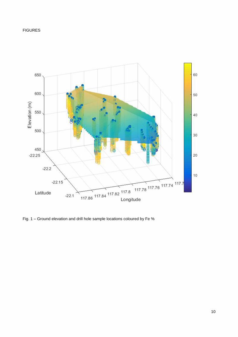
In the case study dataset, it was found that 30% of samples contained errors such as missing values or

mineral grade values that were negative. Upon further investigation the negative mineral grade values where

very small and could be attributed to sensor noise. In this case the samples were kept and the negative

values were set to zero. As a result, approximately 15% of samples were removed from the dataset. As seen

in Fig. 1 a surface is fitted to the starting location of the holes using Curve Fitting Toolbox™. The surface fit

highlighted that one of the drill hole starting locations is at a significant offset to the others. In this case the

model of the surface was used to propose a more suitable starting elevation for this drill hole. In this case

both the Easting and Westing was assumed to be correct.

Geological Formation and Domain Identification

A geological domain represents an area or volume within which the characteristics of the mineralization are

more similar than outside the domain (Glacken & Snowden, 2001). This grouping of drill hole samples by

mineralization is an ideal task for machine learning as the technique is well suited for identifying patterns in

data. The identification of discrete sets of data is known as classification in the context of machine learning.

Initially, unsupervised machine learning is applied as there is no training data with a known relationship

between the mineralization and the geological domain. This process of unsupervised learning would be ideal

for early stages of exploration. As the project matures and further drill hole surveying is performed, or a

geoscientist identifies domains, supervised machine learning techniques can then be applied. In this case

the known samples are used to train models that characterise the mineralization for each domain. These

models are then used to classify subsequent unseen or new drill hole samples. The application of this

workflow will be highlighted as part of a later section on model verification. The procedure was developed

using MATLAB and Statistics and Machine Learning Toolbox™.

5

The initial application of unsupervised machine learning uses a technique known as clustering. In this case it

takes the mineral grades as an input and then identifies groups within the data that display similar

characteristics. The clustering algorithm takes the absolute difference between points in n-dimensional

space and their respective closest cluster central point. Each cluster represents a group or a geological

domain in this context. There can be any number of clusters greater than two. The algorithm then moves the

cluster central points to minimise the sum of these distances. In this application the n-dimensional space is

defined by the number of input mineral grades.

The successful application of this technique requires the selection of the data set, number of clusters, and

correct normalization of the input data. In this paper all the samples that were deemed valid were used as

clustering input. The number of domains was selected by evaluating clustering with different numbers of

domains and selecting the one that provided good performance. Performance was evaluated by using an

output from the MATLAB silhouette routine which identifies the strength of a cluster. A strong cluster is

where all points are close together and relatively far away from other clusters. The opposite is true for a

weak cluster. It is typical to normalise the input data to the same absolute range so they have equal impact

to the clustering. Alternatively, weighting can be applied to bias the influence of some input mineral grades.

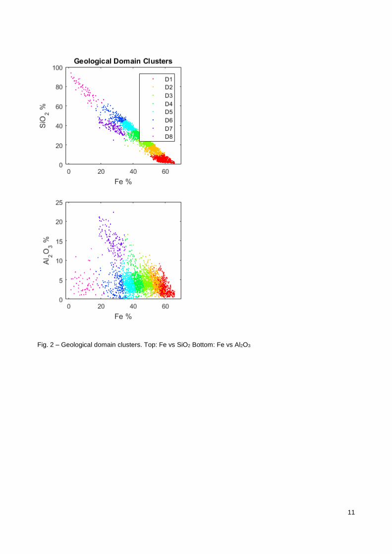
In this case study the best performance was achieved by not normalizing the input data and allowing larger

mineral percentage of Fe and SiO2 to have a greater influence on the clustering algorithm. In part this is

because the grade of Fe is a good predictor of ore grade and SiO2 is negatively correlated to Fe. In contrast,

the other minerals show a weaker correlation to Fe. As it is very difficult to visualise n-dimensional space, the

clustering performance is best visualised using a series of 2-dimension scatter plots of the dominating

factors such as Fe vs SiO2 and Fe vs P shown in Fig. 2. The mineralization of each domain is clearly

grouped when reviewing the distribution of grades that is assigned to each domain. The ability of the

clustering to correctly identify the geological formations and domains can be seen by focusing on three drill

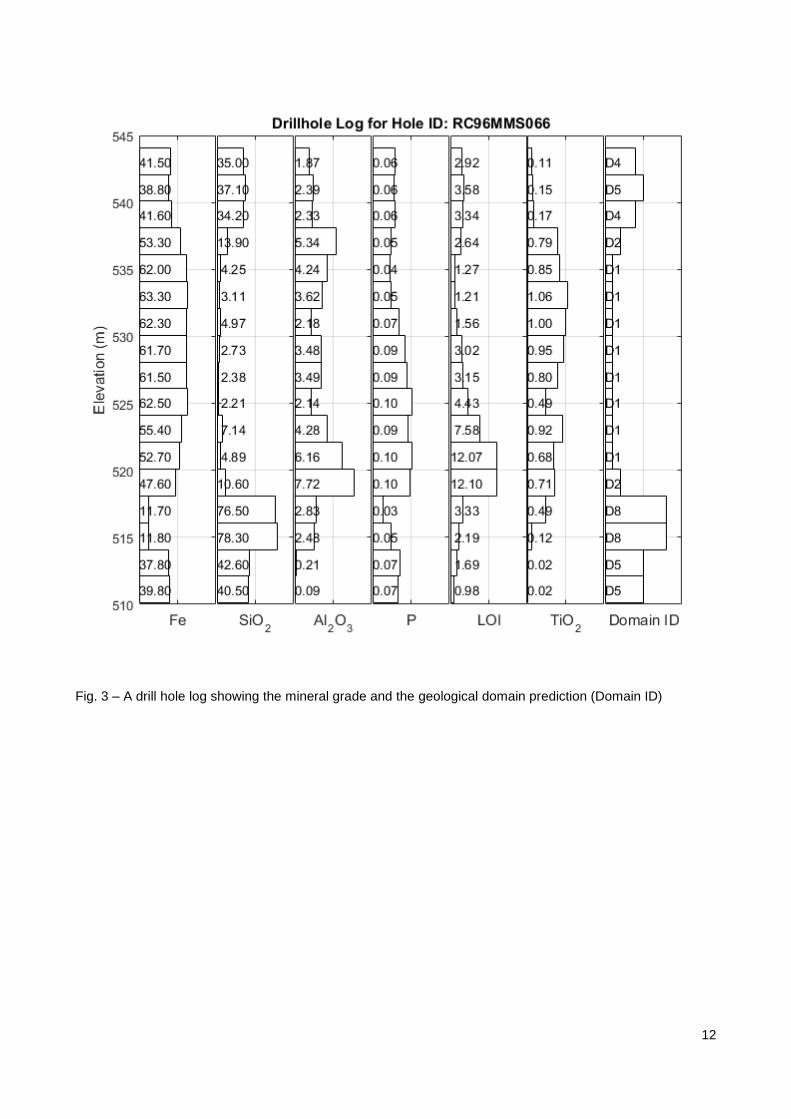
holes, which contain a number of high grade samples shown using a cross-sectional cut through in Fig. 4.

Fig. 3 contains a detail view for one of these drill holes with mineral grades and classified domain

(DomainID) shown for each sample. It has correctly identified a low grade formation (that includes domains

D3 through D6) and the boundary to a higher product grade formation below (that includes D1 and D2). It

has also identified the resource basement that is a thin layer of low grade material (that includes D7 and D8)

directly below the higher quality formation. The hard boundaries between the domains that span the three

drill holes are identified in Fig. 4.

In this example only the grade information was used to identify the domains. Improvements would be

realised if other sources of information were included such as infrared mineralogy as highlighted in Haest

(Haest, et al., 2015). Drill hole absolute position could also provide further value in identifying clusters of

samples that are located close together.

Resource Modelling to Determine Value and Risk

The resource model is fundamental in estimating the value of the resource. Conditional simulation applies

Monte Carlo techniques to generate many realizations or models of an orebody. This allows uncertainty and

risk around the total ore value, and delivered product grade to be assessed. Dimitrakopoulos

6

(Dimitrakopoulos, 1998) provides an overview of the various conditional simulation algorithms. In this paper

the sequential Gaussian simulation (SGS) was implemented using MATLAB and Statistics and Machine

Learning Toolbox. The procedure applied to this case study and detailed by others (Gao, 2015b) (Gao,

2015a) is as follows:

1. Transform sample data to normal-score data with zero mean and unit variance.

2. Randomly select a discrete location within the resource (or node) to be simulated.

3. Calculate the local conditional probability distribution (LCPD) using kriging.

4. Select a value at random from the LCPD.

5. Include the new value as part of the conditioning data.

6. Repeat steps 2-6 until all grid nodes have been assigned a value.

7. Back-transform the realization into the original space.

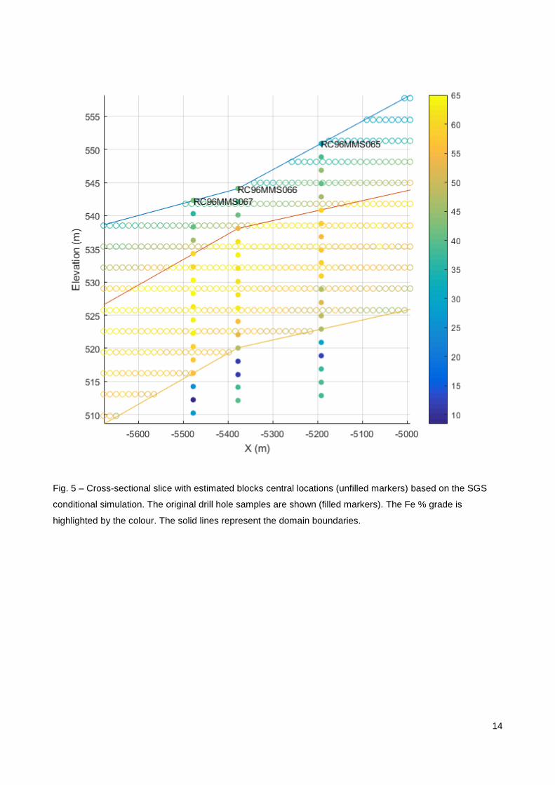
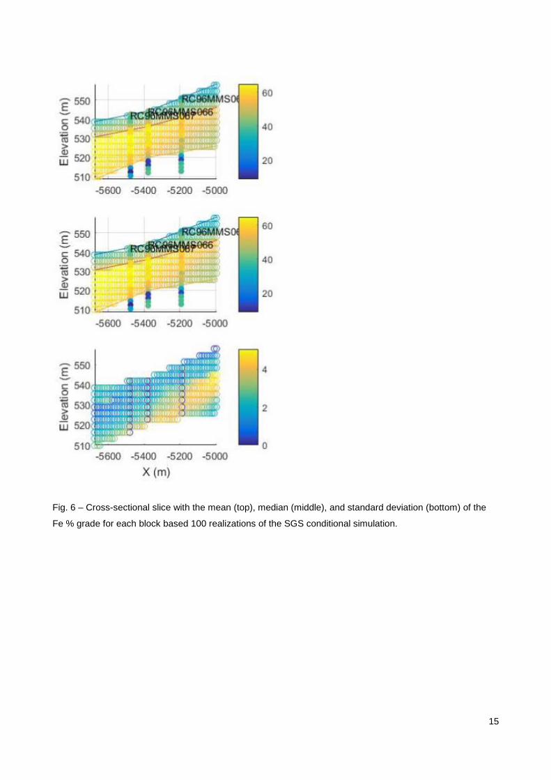
The SGS was applied to the region highlighted in the previous section. The block model for a single

realization is shown in Fig. 5. The mean, median, and standard deviation for each node location of all 100

simulations is (SPE International, 2015) shown in Fig. 6. Large differences between the mean and median

indicate that the results are skewed and more realizations are required. Regions of large standard deviation

highlight areas of uncertainty that may need to be resolved by further drilling and sampling in these regions.

One drawback of SGS is that it is computationally expensive as the LCPD needs to be calculated for each

block that is estimated and many independent simulation runs need to be performed to understand

uncertainty in the model. To accelerate calculation of the different realizations from the various simulations, a

computational cluster with 12 machines, each with four cores, was accessed using Parallel Computing

Toolbox™. This allowed 48 independent simulations to be run simultaneously and subsequently sped up the

calculation. The development was done on a single mineral for a single realization. Once verified, it was a

small step to scale this up to many realizations for many minerals using this computational cluster.

As each mineral is estimated independently there is a risk of generating blocks that no longer represent the

original intended domain or are infeasible. Possible improvements to this process could be achieved if a

multivariate model of the mineralization of each domain was used to generate each block grade. In absence

of using a multivariate model each block mineralization should be verified.

Resource Model Verification

Verification is required as each element is simulated independently and therefore departures from the

domains stratigraphy could be introduced, or the mineral composition might not be feasible as the sum of the

mineral percentages is greater than 100%. Whilst determining the sum of block grades requires a simple

calculation, it is more complex to determine if a generated block represents the stratigraphy of the intended

domain. To conduct this verification step a model that predicts the geological domain from the sample or

block grade mineralization is required. This model includes the correlation effects between minerals such as

7

Fe and SiO2 shown in Fig. 2. As the original drill hole sample data and geological domain results were

generated as part of the domaining step, they can be used to train a supervised machine learning model.

The inputs (predictors) will be the mineral grades and the output (response) will be the domain. Once again

this is a machine learning classification routine as it is identifying membership of a drill hole sample to a

discrete domain. The procedure was developed using MATLAB and Statistics and Machine Learning

Toolbox. The modelling process was accelerated through the use of the graphical user interface of the

Classification Learner application that can be found within these tools.

A series of models was developed using the many machine learning classification algorithms available

including decision trees, discriminant analysis, support vector machines, nearest neighbour classifiers, and

ensemble classifiers. The performance of each of the models was evaluated using 5-fold cross validation.

The 5-fold cross validation provides a high level of model assurance as it trains and tests a model 5 times

using different combinations of the dataset for testing and training each time. The Bagged Tree ensemble

classifier, an algorithm that takes the results from a number of binary trees and then aggregates them

together to provide a prediction, provided the best performance. This algorithm provides metrics that allow

the modeller to assess the relative impact that each mineral grade (predictor) has on the geological domain

prediction (response). In this case study SiO2, Fe, Al2O3, and TiO2 were relatively important predictors. This

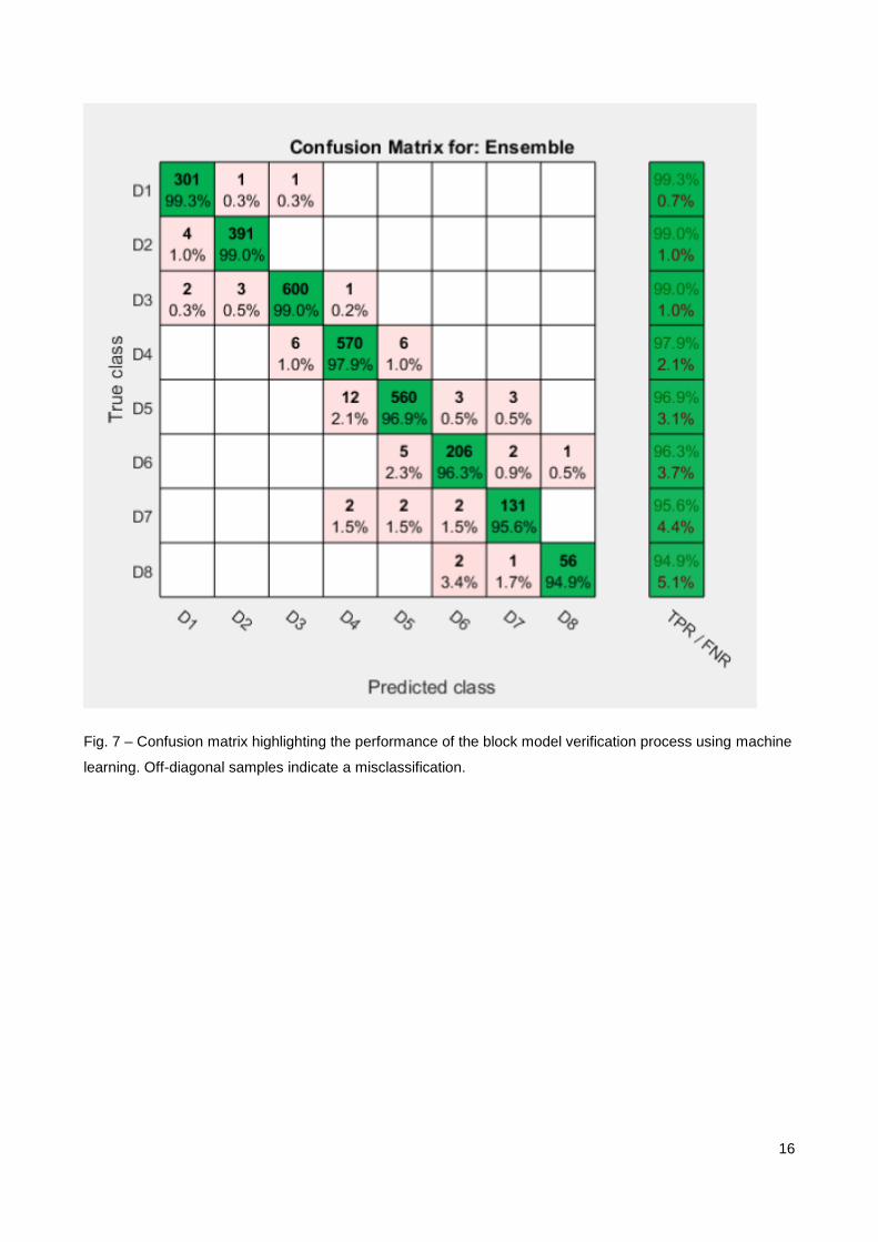
generated model is then used to predict the domain of each block within the generated SGS realization given

the block mineral grades. Fig. 7 shows a confusion matrix that plots the intended domain against the model-

predicted domain. Using this visualisation, misclassification can be identified through-off diagonal

predictions. The algorithm had an excellent prediction accuracy of 98%, confirming that the majority of blocks

generated by the SGS conforms to the predicted mineralogy of the domain. The misclassification rate was

2%. Predominately these misclassified samples were assigned to neighbouring domains and therefore

represent the model uncertainty when samples are located close to the boundary between two domains.

Despite the excellent results, the model development process could be further refined. Model reduction

techniques to remove the minerals with low feature importance is a common workflow that allows simpler,

and subsequently more general and robust, models to be generated. Other model reduction techniques that

provide similar benefits but are specific to the Bagged Tree algorithm include parameters that reduce the

size of the tree.

CONCLUSIONS

Automation through the application of machine learning to the development of a resource model is a

promising technique to complement the current industry best practices. The automation provided by the

machine learning techniques in both identification of the geological domains and verification of the correct

mineralization of model developed using conditional simulation can provide many benefits. This includes

accelerating the pace of resource value estimation to allow quicker turn around in the exploration process

and the ability for the model to be regenerated to evaluate different assumptions or to changes in the input

data. Automation provides subsequent benefits in that it allows the expert geologist to spend more time to

monitor, refine, and innovate to improve the processes, as opposed to manually performing the domaining

operations on hundreds of drill holes and thousands of samples, a process that is not easily scalable.

8

Application of the process to an existing orebody where the domains are known would allow further

validation of the process and would provide insight into future directions in applying machine learning to this

field.

ACKNOWLEDGEMENTS

I would like to acknowledge MathWorks for allowing me to publish on this topic. I would also like to

acknowledge the Government of Western Australia, Department of Mines and Petroleum for providing a rich

resource in the form of the Company Mineral Drillhole Database (CMDD) (Government of Western Australia,

Department of Mines and Petroleum, 2015).

REFERENCES Dimitrakopoulos, R., 1998. Conditional simulation algorithms for modelling orebody uncertainty in open pit optimisation. International Journal of Surface Mining Reclamation and Environment, pp. 173-178.

Dimitrakopoulos, R., Martinez, L. & Ramazan, S., 2007. A maximum upside / minimum downside approach to the traditional optimization of open pit mine design. Journal of Mining Science, pp. 73-82.

Gao, Y., 2015a. What is a Normal Score Transformation?. [Online] Available at: http://www.knowledgette.com/9KTE/what-is-a-normal-score-transformation/

Gao, Y., 2015b. What is Sequential Gaussian Simulation?. [Online] Available at: http://www.knowledgette.com/fUQ/what-is-sequential-gaussian-simulation/

Glacken, I. M. & Snowden, D. V., 2001. Mineral Resource Estimation. In: Mineral Resource and Ore Reserve Estimation - The AusIMM Guide to Good Practice. Melbourne: The Australiasian Institute of Mining and Metallurgy, pp. 189-198.

Government of Western Australia, Department of Mines and Petroleum, 2015. Company Mineral Drilhole Data and Surface Geochemistry. [Online] Available at: http://www.dmp.wa.gov.au/Company-mineral-drill-hole-data-1552.aspx

Haest, M., Mittrup, D. & Dominguez, O., 2015. Reaping the First Fruits – Infrared Spectroscopy: the New Standard Tool in BHP Billiton Iron Ore Exploration. Perth, The Australasian Institute of Mining and Metallurgy: Melbourne, p. pp 277–284 .

MathWorks, 2015. Machine Learning with MATLAB. [Online] Available at: http://www.mathworks.com/solutions/machine-learning/

Morley, C., 1999. Financial impact of resource/reserve uncertainty. The Journal of The South African Institute of Mining and Metallurgy, pp. 293-302.

Russakovsky, O. et al., 2015. ImageNet Large Scale Visual Recognition Challenge. International Journal of Computer Vision (IJCV), Volume 115, pp. 211-252.

SPE International, 2015. Geostatistical conditional simulation. [Online] Available at: http://petrowiki.org/Geostatistical_conditional_simulation#Static_displays_of_uncertainty

9

FIGURE CAPTIONS

Fig. 1 – Ground elevation and drill hole sample locations coloured by Fe %

Fig. 2 – Geological domain clusters. Top: Fe vs SiO2 Bottom: Fe vs Al2O3

Fig. 3 – A Drill hole log showing the mineral grade and the geological domain prediction (Domain ID)

Fig. 4 – Cross-sectional slice with the geological domains for each sample highlighting the colour (1 to 8 is

high through to low quality domains) and the boundaries between these domains

Fig. 5 – Cross-sectional slice with estimated blocks central locations (unfilled markers) based on the SGS

conditional simulation. The original drill hole samples are shown (filled markers). The Fe % grade is

highlighted by the colour. The solid lines represent the domain boundaries.

Fig. 6 – Cross-sectional slice with the mean (top), median (middle), and standard deviation (bottom) of the

Fe % grade for each block based 100 realizations of the SGS conditional simulation.

Fig. 7 – Confusion matrix highlighting the performance of the block model verification process using machine

learning. Off-diagonal samples indicate a misclassification.

10

FIGURES

Fig. 1 – Ground elevation and drill hole sample locations coloured by Fe %

11

Fig. 2 – Geological domain clusters. Top: Fe vs SiO2 Bottom: Fe vs Al2O3

12

Fig. 3 – A drill hole log showing the mineral grade and the geological domain prediction (Domain ID)

13

Fig. 4 – Cross-sectional slice with the geological domains for each sample highlighting the colour (1 to 8 is

high through to low quality domains) and the boundaries between these domains.

14

Fig. 5 – Cross-sectional slice with estimated blocks central locations (unfilled markers) based on the SGS

conditional simulation. The original drill hole samples are shown (filled markers). The Fe % grade is

highlighted by the colour. The solid lines represent the domain boundaries.

15

Fig. 6 – Cross-sectional slice with the mean (top), median (middle), and standard deviation (bottom) of the

Fe % grade for each block based 100 realizations of the SGS conditional simulation.

16

Fig. 7 – Confusion matrix highlighting the performance of the block model verification process using machine

learning. Off-diagonal samples indicate a misclassification.