development of benchmark examples for static delamination propagation and fatigue ... · ·...

DEVELOPMENT OF BENCHMARK EXAMPLES FOR STATIC DELAMINATION PROPAGATION AND FATIGUE GROWTH PREDICTIONS

Ronald Krueger*

ABSTRACT

The development of benchmark examples for static delamination propagation and cyclic delamination onset and growth prediction is presented and demonstrated for a commercial code. The example is based on a finite element model of an End-Notched Flexure (ENF) specimen. The example is independent of the analysis software used and allows the assessment of the automated delamination propagation, onset and growth prediction capabilities in commercial finite element codes based on the virtual crack closure technique (VCCT). First, static benchmark examples were created for the specimen. Second, based on the static results, benchmark examples for cyclic delamination growth were created. Third, the load-displacement relationship from a propagation analysis and the benchmark results were compared, and good agreement could be achieved by selecting the appropriate input parameters. Fourth, starting from an initially straight front, the delamination was allowed to grow under cyclic loading. The number of cycles to delamination onset and the number of cycles during stable delamination growth for each growth increment were obtained from the automated analysis and compared to the benchmark examples. Again, good agreement between the results obtained from the growth analysis and the benchmark results could be achieved by selecting the appropriate input parameters. The benchmarking procedure proved valuable by highlighting the issues associated with the input parameters of the particular implementation. Selecting the appropriate input parameters, however, was not straightforward and often required an iterative procedure. Overall, the results are encouraging but further assessment for mixed-mode delamination is required.

1. INTRODUCTION

Over the past two decades, the use of fracture mechanics has become common practice to characterize the onset and growth of delaminations. In order to predict delamination onset or growth, the calculated strain energy release rate components are compared to interlaminar fracture toughness properties measured over a range from pure mode I loading to pure mode II loading.

The virtual crack closure technique (VCCT) is widely used for computing energy release rates based on results from continuum (2D) and solid (3D) finite element (FE) analyses and to supply the mode separation required when using the mixed-mode fracture criterion [1, 2]. The virtual crack closure technique was recently implemented into several commercial finite element codes. As new methods for analyzing composite delamination are incorporated into finite element codes, the need for comparison and benchmarking becomes important since each code requires specific input parameters unique to its implementation.

An approach for assessing the delamination propagation capabilities in commercial finite element codes under static loading was recently presented and demonstrated for VCCT for ABAQUS®1 [3] as well as MD Nastran™ and Marc™2 [4]. First, benchmark results were created

*R. Krueger, National Institute of Aerospace, 100 Exploration Way, Hampton, VA, 23666, resident at Durability, Damage Tolerance and Reliability Branch, MS 188E, NASA Langley Research Center, Hampton, VA, 23681, USA. 1 ABAQUS® is a product of Dassault Systèmes Simulia Corp. (DSS), Providence, RI, USA

1

https://ntrs.nasa.gov/search.jsp?R=20110011430 2018-07-02T16:01:54+00:00Z

manually for full three-dimensional finite element models of the Double Cantilever Beam (DCB) and the Single Leg Bending (SLB) specimen. Second, starting from an initially straight front, the delamination was allowed to propagate using the automated procedure implemented in the finite element software. The approach was then extended to allow the assessment of the delamination fatigue growth prediction capabilities in commercial finite element codes [5]. As for the static case, benchmark result were created manually first. Second, the delamination was allowed to grow under cyclic loading in a finite element model of a commercial code. In general, good agreement between the results obtained from the propagation and growth analysis and the benchmark results could be achieved by selecting the appropriate input parameters. Overall, the results were encouraging but showed that additional assessment for mode II and mixed-mode delamination is required.

The objective of the present study was to create additional benchmark examples, independent of the analysis software used, which allows the assessment of the static delamination propagation as well as the onset and growth prediction capabilities in commercial finite element codes. For the simulation of mode II fracture, the three-point bending End Notched Flexure (ENF) specimen was selected as shown in Figure 1. Dimensions, layup and material properties were taken directly from a related experimental study [6]. To avoid unnecessary complications, experimental anomalies such as fiber bridging in mode I were not addressed in the simulation.

Static benchmark results were created based on the approach developed earlier [3], using two-dimensional finite element models for simulating the ENF specimens with different delamination lengths a0. For each delamination length modeled, the load, Q, and the center deflection, w, were monitored. The mode II strain energy release rate, GII, was calculated for a fixed applied load. It is assumed that the delamination propagates when computed energy release rate, GII, reaches the fracture toughness GIIc. Thus, critical loads and critical displacements for delamination propagation were calculated for each delamination length modeled. From these critical load/displacement results, benchmark solutions were created. It is assumed that the load/displacement relationship computed during automatic propagation should closely match the benchmark cases.

Benchmark cases to assess the growth prediction capabilities were created based on the finite element models of the ENF specimen used for the static benchmark case. First, the number of cycles to delamination onset, ND, was calculated from the mode II fatigue delamination growth onset data of the material [6]. Second, the number of cycles during stable delamination growth, ΔNG, was obtained incrementally from the material data for mode II fatigue delamination propagation [6] by using growth increments of Δa=0.1 mm. Third, the total number of growth cycles, NG, was calculated by summing over the increments ΔNG. Fourth, the corresponding delamination length, a, was calculated by summing over the growth increments Δa. Finally, for the benchmark case where results for delamination onset and growth were combined, the delamination length, a, was calculated and plotted versus an increasing total number of load cycles NT=ND+NG.

After creating the benchmark cases, the approach was demonstrated for the commercial finite element code ABAQUS®. Starting from an initially straight front, the delamination was allowed to propagate under static loading or grow under cyclic loading based on the algorithms implemented into the software. Input control parameters were varied to study the effect on the computed delamination propagation and growth. The benchmark enabled the selection of the appropriate input parameters that yielded good agreement between the results obtained from the growth analysis and the benchmark results. Once the parameters have been identified, they may then be used with confidence to model delamination growth for more complex configurations. 2 MD Nastran™ and Marc™ are manufactured by MSC.Software Corp., Santa Ana, CA, USA. NASTRAN® is a registered trademark of NASA.

2

In the paper, the development of the benchmark cases for the assessment of the static delamination propagation as well as the onset and growth prediction capabilities are presented. Examples of automated propagation and growth analyses are shown, and the selection of the required code specific input parameters are discussed.

2. SPECIMEN AND MODEL DESCRIPTION 2.1 Mode II End-Notched Flexcure (ENF) specimen

For the current numerical investigation, the three-point End-Notched Flexure (ENF) specimen, as shown in Figure 1, was chosen since it is simple, only exhibits the mode II opening fracture mode and had been used previously to develop an approach to assess the quasi-static delamination propagation simulation capabilities in commercial finite element codes [4]. The methodology for delamination propagation, onset and growth was applied to the ENF specimen to create the benchmark example [7, 8]. For the current study, an ENF specimen made of IM7/8552 graphite/epoxy with an unidirectional layup, [0]24, was modeled. The material, layup, overall specimen dimensions including initial crack length, a, were identical to specimens used in a related experimental study [6]. The material properties are given in Tables I and II. 2.2 Finite element models

A typical two-dimensional finite element model of an End-Notched Flexure (ENF) specimen with boundary conditions is shown in Figure 2. The specimen was modeled with solid plane strain elements (CPE4, CPE4I) and solid plane stress elements (CPS4) in ABAQUS® Standard 6.9EF and 6.10. Along the length, all models were divided into different sections with different mesh refinement. The ENF specimen was modeled with six elements through the specimen thickness (2h). The resulting element length at the delamination tip was Δa=1.0 mm. Finer meshes, resulting in Δa=0.5 mm and Δa=0.25 mm were also generated and are discussed in detail in a related report [9].

The plane of delamination was modeled as a discrete discontinuity in the center of the specimen. For the analysis with ABAQUS® 6.9EF and 6.10, the models were created as separate meshes for the upper and lower part of the specimens with identical nodal point coordinates in the plane of delamination [10]. Two surfaces (top and bottom surface) were defined to identify the contact area in the plane of delamination as shown in Figure 2. Additionally, a node set was created to define the intact (bonded nodes) region.

A typical three-dimensional finite element model of the ENF specimen is shown in Figure 3. Along the length, all models were divided into different sections with different mesh refinement. A refined mesh was used in the center of the ENF specimen. Across the width, a uniform mesh (25 elements) was used to avoid potential problems at the transition between a coarse and finer mesh [3-5]. Through the specimen thickness (2h), six elements were used. The resulting element length at the delamination tip was Δa=1.0 mm. The specimen was modeled with solid brick elements (C3D8I), which had yielded excellent results in a previous studies [3.4]. Refined models, as well as models with model continuum shell elements (SC8R) were also generated and are discussed in detail in a related report [9].

3

2.3 Analysis tools 2.3.1 Static delamination propagation analysis

For the automated delamination propagation analysis, the VCCT implementation in ABAQUS® Standard 6.9EF and 6.10 were used. The plane of delamination in three-dimensional analyses is modeled using the existing ABAQUS®/Standard crack propagation capability based on the contact pair capability [10]. Additional element definitions are not required, and the underlying finite element mesh and model does not have to be modified [10]. The implementation offers a crack and delamination propagation capability in ABAQUS®. It is implied that the energy release rate at the crack tip is calculated at the end of a converged increment. Once the energy release rate exceeds the critical strain energy release rate (including the user-specified mixed-mode criteria as shown in Figure 2), the node at the crack tip is released in the following increment, which allows the crack to propagate. To avoid sudden loss of stability when the crack tip is propagated, the force at the crack tip before advance is released gradually during succeeding increments in such a way that the force is brought to zero no later than the time at which the next node along the crack path begins to open [10].

In addition to the mixed-mode fracture criterion, VCCT for ABAQUS® requires additional input for the propagation analysis. If a user specified release tolerance is exceeded in an increment

€

(G −Gc ) /Gc > release tolerance, a cutback operation is performed which reduces the time increment. In the new smaller increment, the strain energy release rates are recalculated and compared to the user specified release tolerance. The cutback reduces the degree of overshoot and improves the accuracy of the local solution [10]. A release tolerance of 0.2 is suggested in the handbook [10].

To help overcome convergence issues during the propagation analysis, ABAQUS® provides:

• contact stabilization which is applied across only selected contact pairs and used to control the motion of two contact pairs while they approach each other in multi-body contact. The damping is applied when bonded contact pairs debond and move away from each other [10]

• automatic or static stabilization which is applied to the motion of the entire model and is commonly used in models that exhibit statically unstable behavior such as buckling [10]

• viscous regularization which is applied only to nodes on contact pairs that have just debonded. The viscous regularization damping causes the tangent stiffness matrix of the softening material to be positive for sufficiently small time increments. Viscous regularization damping in VCCT for ABAQUS® is similar to the viscous regularization damping provided for cohesive elements and the concrete material model in ABAQUS®/Standard [10]. Further details about the required input parameters are discussed in a related report [9].

For automated propagation analysis, it was assumed that the computed behavior should closely match the benchmark results created below. For all analyses, the elastic constants (given in Table I), and the input to define the fracture criterion (given in Table II) were kept constant. The following items were changed to study the effect on the automated delamination propagation behavior during the analysis:

• The release tolerance (reltol) was varied. • The input for contact stabilization (cs) was varied. • The input for viscous regularization (damv) was varied. • Two- and three dimensional models with different types of elements were used. • Models with different element length at the crack tip/delamination front, Δa, were used.

4

2.3.2 Fatigue delamination onset and growth analysis For the automated delamination onset and growth analysis, the low-cycle fatigue analysis in

ABAQUS® Standard 6.9EF and 6.10 was used to model delamination growth at the interfaces in laminated composites [10]. A direct cyclic approach is part of the implementation and provides a computationally effective modeling technique to obtain the stabilized response of a structure subjected to constant amplitude cyclic loading. The theory and algorithm to obtain a stabilized response using the direct cyclic approach are described in detail in reference 10. Delamination onset and growth predictions are based on the calculation of the strain energy release rate at the delamination front using VCCT. To determine propagation, computed energy release rates are compared to the input data for onset and growth from experiments as discussed in the methodology section. The implementation is set up to release at least one element at the interface after the loading cycle is stabilized [10].

For automated delamination onset and growth analyses, it was assumed that the computed behavior should closely match the benchmark results created below. For all analyses, the elastic constants (given in Table I), the input to define the fracture criterion (given in Table II), and the parameters for delamination onset and delamination growth (Paris Law) (given in Table II) were kept constant. The parameters to define the load frequency (f=5 Hz), the load ratio (R=0.1) as well as the minimum and maximum applied displacement (wmin and wmax) were also kept constant during all analyses. A Fourier series is used during the execution of the ABAQUS® Standard to approximate the periodic cyclic loading. Based on previous results, it was decided to use 50 Fourier terms to approximate the periodic cyclic loading [5]. Further details about the required input parameters are discussed in a related report, where a sample input file is also provided [9]. The following items were changed to study the effect on the predicted delamination onset and growth behavior during the analysis:

• The input to define the cyclic loading was studied. The starting time, t0, which causes

a phase-shift was varied. • Two- and three dimensional models with different types of elements were used. • For three-dimensional models, the number of terms used to define a Fourier series

was reduced to decrease computation time. • Models with different element length at the crack tip/delamination front, Δa, were used.

3. CREATING BENCHMARK SOLUTIONS 3.1 Development of a Benchmark Example for Static Loading

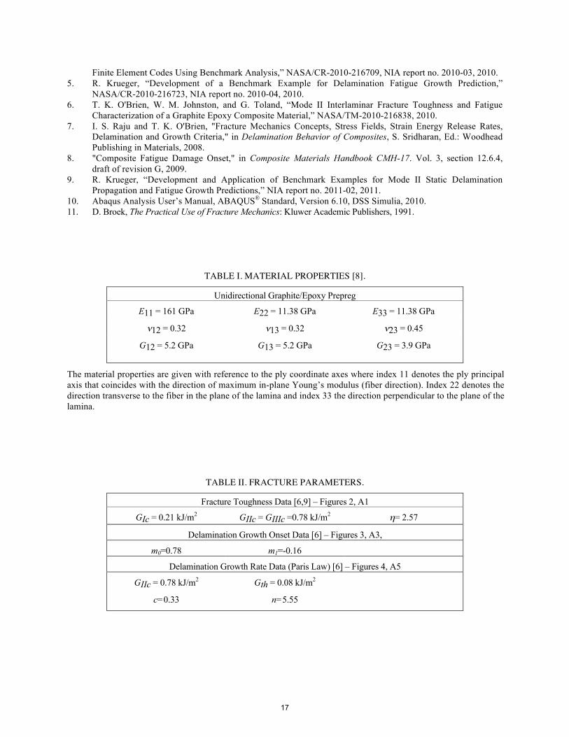
The static benchmark case was created based on an approach developed earlier [3]. Two-dimensional finite element models simulating ENF specimens with 15 different delamination lengths a0 were created (25.4 mm≤ a0.≤76.2 mm). For each delamination length modeled, the load, Q, and center deflection, w, were monitored as shown in Figure 4 (colored lines). Using VCCT, the mixed-mode strain energy release rate components were computed for the applied load Q=2000 N. As expected, the results were predominantly mode II and were included in the plot of Figure 4. Therefore, a failure index GII/GIIc was calculated by correlating the results with the mode II fracture toughness, GIIc, of the graphite/epoxy material. It is assumed that the delamination propagates when the failure index reaches unity. Therefore, the critical load, Qcrit, can be calculated based on the relationship between load, Q, and the energy release rate, G, [11]

5

€

G =Q2

2⋅∂CP

∂A . (1)

In equation (1), CP is the compliance of the specimen, and ∂A is the increase in surface area

corresponding to an incremental increase in load or displacement at fracture. The critical load, Qcrit, and critical displacement, wcrit, were calculated for each delamination length modeled

€

GII

GIIc

=Q2

Qcrit2 ⇒ Qcrit =Q GIIc

GII

, wcrit = w GIIc

GII

(2)

and the results were included in the load/displacement plots as shown in Figure 4 (solid red circles). These critical load/displacement results indicated that, with increasing delamination length, less load is required to extend the delamination. At the same time, the values of the critical center deflection decreased. This means that the ENF specimen exhibits unstable delamination propagation under load as well as displacement control (solid red line).

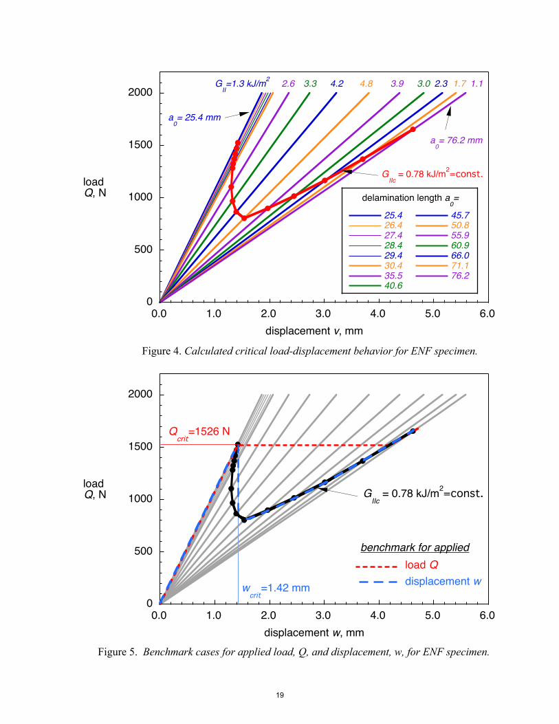
From these critical load/displacement results, two benchmark solutions can be created as shown in Figure 5. During the analysis, either prescribed center deflections, w, or nodal point loads, Q, are applied. For the case of prescribed center deflections, w, (long dashed blue line), the applied displacement must be held constant over several increments once the critical point (Qcrit, vcrit) is reached, and the delamination front is advanced during these increments. Once the critical path (solid black circles and solid black line) is reached, the applied center deflection is increased again incrementally. For the case of applied nodal point loads (short dashed red line), the applied load must be held constant while the delamination front is advanced during these increments. Once the critical path (solid black circles and solid black line) is reached, the applied load is increased again incrementally. It is assumed that the load/displacement, relationship computed during automatic propagation should closely match the benchmark cases. 3.2 Development of a benchmark example for delamination onset and growth prediction

For the development of the benchmark case for delamination onset and growth under cyclic loading, guidance was taken from test results for mode II interlaminar fracture toughness and fatigue characterization [6]. In the report, a series of tests are documented which were conducted under load control with a maximum load, Qmax, which caused the energy release rate at the front, GIImax, to reach values of 50% of GIIc

€

GIImax

GIIc

= 0.5 (3)

The maximum load, Q50,max, and the maximum center deflection, w50,max, were calculated using

the known quadratic relationship between energy release rate and applied load or displacement

€

GIImax

GIIc

=Qmax

2

Qcrit2 ⇒ Qmax =Qcrit

GIImax

GIIc

, wmax = wcritGIImax

GIIc

(4)

€

Qmax =Qcrit 0.5 , wmax = wcrit 0.5 (5)

6

where Qcrit and wcrit are the critical values. For the current study, a critical energy release rate GIIc=0.78 kJ/m2 was used, and the critical values, Qcrit, (solid red horizontal line) and, wcrit, (solid red vertical line) were obtained from the benchmark for static delamination propagation (discussed above) shown in the load-displacement plot in Figure 6. The calculated maximum load, Q50,max, and calculated maximum displacement, w50,max, are shown in Figure 6 (long dashed red lines) in relationship to the static benchmark case (solid grey circles and dashed grey line) mentioned above. During constant amplitude cyclic loading of an ENF specimen under load control, the applied maximum load, Q50,max=1079 N, is kept constant while the displacement increases with increasing delamination length (horizontal dashed red line). For simulations preformed under displacement control, the applied maximum displacement, w50,max=1.0 mm, is kept constant while the load decreases as the delamination length increases (vertical dashed red line). In the report, tests are also documented that were performed at 40%, 30% and 20% of GIIc [6]. The corresponding maximum loads and the maximum center deflections values were calculated using equation (4) and were included in the plot of Figure 6 (Q40,max, Q30,max, Q20,max - horizontal lines; w40,max, w30,max, w20,max – vertical lines).

The energy release rate corresponding to an applied load, Q50,max=1079 N, was calculated for different delamination lengths, a, using equation (4). The energy release rate first increased with increasing delamination length, a, as shown in Figure 7 (open red circles and dashed red line). After reaching a peak, the energy release rate decreased with increasing delamination length. Delamination growth was assumed to become unstable once the calculated energy release rate passed the fracture toughness value GIIc (solid blue line in Figure 7). Later, delamination growth was assumed to become stable again after the calculated energy release rate dropped below the fracture toughness value GIIc. Additionally, the energy release rate dependence on the crack length, a, was calculated for Q40,max, Q30,max, and Q20,max, and the results were included in the plot of Figure 7 (dashed lines with open symbols). The static benchmark case (solid grey circles and dashed grey line in Figure 7), where the delamination propagates at constant GIIc (solid blue line in Figure 7) was included for comparison. Also included was the cutoff (threshold) value, Gth, (green solid horizontal line) below which growth is assumed to stop.

The energy release rate corresponding to an applied center deflection, w50,max=1.0 mm, was also calculated for different delamination lengths, a, using equation (4). The energy release rate first increased with increasing delamination length, a, as shown in Figure 8 (solid red circles and dashed red line). After reaching a peak, the energy release rate decreased with increasing delamination length. Delamination growth was assumed to stop once the calculated energy release rate dropped below the cutoff value, Gth, (green solid horizontal line). Additionally, the energy release rate dependence on the crack length, a, was calculated for w40,max, w30,max, and w20,max, and the results were included in the plot of Figure 8 (dashed lines with solid symbols). The static benchmark case (solid grey circles and dashed grey line in Figure 8), where the delamination propagates at constant GIIc (solid blue line in Figure 8) was included for comparison. 3.2.1 Fatigue delamination growth onset

The number of cycles to delamination onset, ND, can be obtained from the delamination onset curve which is a power law fit of experimental data obtained from a ENF test using the respective standard for delamination growth onset. Details are discussed in a related report [9]. Solving for ND yields

7

€

G = m0 ⋅NDm1 ⇒ ND =

1m0

1m1

c1

⋅G1m1 ⇒ ND = c1 ⋅G

c2 (6)

€

where c2 =1m1

. Values for the constants c1 and c2 are given in Table II.

At the beginning of the test, the specimen is loaded initially so that the energy release rate at the front, GII, reaches about 50% of GIIc corresponding to G50=0.392 kJ/m2. From the delamination onset curve, the number of cycles to delamination onset is determined as, ND50=80. The values corresponding to 40%, 30% and 20% of GIIc were calculated using equation (6). The results are plotted in Figure 9 (horizontal dashed lines). 3.2.2 Fatigue delamination growth

The number of cycles during stable delamination growth, NG, can be obtained from the fatigue delamination propagation relationship (Paris Law). The delamination growth rate (solid purple line) can be expressed as a power law function

€

dadN

= c ⋅Gmaxn or

€

ΔaΔN

= c ⋅Gmaxn (7)

where da/dN is the increase in delamination length per cycle and Gmax is the maximum energy release rate at the front at peak loading. The factor c and exponent n are obtained by fitting the curve to the experimental data obtained from ENF tests [6]. A cutoff value (threshold), Gth, was chosen below which delamination growth was assumed to stop. Details are discussed in a related report [9].

For the current study, increments of Δa=0.1 mm were chosen. Starting at the initial delamination length, a0=25.4 mm, the energy release rates, Gi,max, were obtained for each increment, i, from the curve fit (open red circles and dashed red line) plotted in Figure 7. These energy release rate values were then used to obtain the increase in delamination length per cycle or growth rate Δa/ΔN from the Paris Law. For all load levels, the number of cycles during stable delamination growth, NG, was calculated by summing the increments, ΔNi,

€

NG = ΔNii=1

k

∑ =1cGi,max

-n ⋅ Δai=1

k

∑ (8)

where k is the number of increments. The corresponding delamination length, a, was calculated by adding the incremental lengths, Δa, to the initial length, a0,

€

a = a0 + Δai=1

k

∑ = a0 + k ⋅ Δa . (9)

The analyses were repeated for the case of applied center deflections, w. The number of cycles

during stable delamination growth, NG, and the corresponding delamination length, a, were also calculated using equations (8) and (9), respectively. The results are plotted in Figure 9 (S-shaped dashed lines). Details are discussed in a related report [9].

8

3.2.3 Combined fatigue delamination onset and growth For the combined case of delamination onset and growth, the total life, NT, may be expressed as

€

NT = ND +NG (10)

where, ND, is the number of cycles to delamination onset and NG, is the number of cycles during delamination growth [8]. For this combined case, the delamination length, a, is plotted in Figure 9 for an increasing number of load cycles, NT, for all load levels (Q50,max, Q40,max, Q30,max, and Q20,max – dashed lines). For the first ND cycles, the delamination length remains constant (horizontal dashed red line for Q50,max), followed by a growth section where - over NG cycles - the delamination length increases following the Paris Law (dashed red line for Q50,max). The total life for applied cyclic center deflections is plotted in Figure 10 for all levels (w50,max, w40,max, w30,max, and w20,max). For the first ND cycles, the delamination length remains constant (horizontal dashed red line for w50,max), followed by a growth section where - over NG cycles - the delamination length increases following the Paris Law (dashed red line for w50,max). Once a delamination length is reached where the energy release rate drops below the assumed cutoff value, Gth, the delamination growth no longer follows the Paris Law (dashed grey line) and stops (horizontal dashed red line for w50,max) as shown in Figure 10. For the applied cyclic center deflections, w50,max, two cutoff values Gth=0.08 kJ/m2 and Gth=0.05 kJ/m2 were assumed resulting in a shift of the cutoff as shown in Figure 10 (horizontal dashed red lines). A delamination length prediction analysis that accounts for delamination fatigue onset as well as stable growth should yield results that closely resemble the plots in Figures 9 and 10. The curve fits can therefore be used as a benchmark as demonstrated later.

4. RESULTS FROM AUTOMATED ANALYSES 4.1 Results from automated propagation analyses 4.1.1 Computed delamination propagation for applied static center deflection

The propagation analysis was performed in two steps using the models shown in Figures 2 and 3 for an initial delamination length, a0=25.4 mm. In the first step, a center deflection w=1.3 mm was applied which equaled nearly the critical center deflection, wcrit=1.42 mm, determined earlier. In the second step, the total prescribed displacement was increased (w=5.0 mm). Automatic incrementation was used with a small increment size at the beginning (5.0 10-3 of the total increment) and a very small minimum allowed increment (10-18 of the total increment) to reduce the risk of numerical instability and early termination of the analysis. The analysis was limited to 1000 increments.

To overcome the convergence problems, the methods implemented in ABAQUS® were used individually to study the effects [10]. Initially, analyses were performed using two-dimensional planar models without stabilization or viscous regularization [10]. Release tolerance values were varied between the default value (reltol=0.2) and 0.5. Using reltol=0.2, 0.3 and 0.4, the load dropped at the critical point, but the center deflection kept increasing with decreasing load as shown in Figure 11 (solid red, blue and green lines, respectively) where the computed resultant force (load, Q) in the center of the ENF specimen is plotted versus the applied center deflection, w. Then, the analysis terminated early due to convergence problems. By increasing the release tolerance - as suggested in the ABAQUS® error in the message (.msg) file – it was possible to complete the analysis without error message as shown in Figure 11 for a release tolerance value 0.5 (solid purple line). As desired, the load dropped at the critical point, however, the center deflection kept

9

increasing with decreasing load. Later, the computed load/displacement path converged to the stable propagation branch of the benchmark result. For the stable path, a saw tooth pattern is observed where the top results are in good agreement with the benchmark result. Based on the results, it was decided to introduce additional stabilization to obtain better agreement with the benchmark case.

Based on problems identified during previous analyses, automated or static stabilization was not used in this study [5]. The results computed when contact stabilization (cs) was added are plotted in Figure 12. For a small stabilization factor (cs=1x10-6) and a release tolerance suggested in the handbook (reltol=0.2) [10], the load dropped, and delamination propagation started shortly after reaching the critical point of the benchmark solution (thin solid red line). The load/displacement path then ran parallel to the constant deflection branch of the benchmark result and followed the stable propagation branch of the benchmark result. To reduce the observed overshoot, the release tolerance was reduced. For a stabilization factor (cs=1x10-6) and release tolerance (reltol=0.1) (dashed blue line), the overshot was reduced, and the computed load/displacement path then ran closer to the constant deflection branch of the benchmark result. Further reducing the release tolerance (reltol=0.01) yielded results that were in excellent agreement with the benchmark for a wide range of stabilization factors (1x10-4≤ cs ≤1x10-8) (solid black, light blue, orange and green lines – on top of each other). For the stable path, a saw tooth pattern was observed where the top results were in good agreement with the benchmark result.

When viscous regularization was added to help overcome convergence issues, a value of 0.2 was used initially for the release tolerance as suggested in the handbook [10]. For a viscosity coefficient (damv=0.1) and a release tolerance of 0.2, the load and displacement overshot the critical point as shown in Figure 13 (solid red line). The load/displacement path then ran parallel to the constant deflection branch of the benchmark result and followed the stable propagation branch of the benchmark result. Lowering the viscosity coefficient (damv=1x10-3) did not improve the results (dashed blue line). Further lowering the viscosity coefficient (damv=1x10-4) reduced the overshoot at the critical point, however, the computed deflection started to increase before the transition between the constant deflection branch and the stable propagation was reached (solid black line). Additional reduction in the viscosity coefficient alone (reltol=0.2 and 1x10-5≤ damv ≤1x10-6) reduced the overshoot and shifted the results closer to the constant deflection branch of the benchmark (dashed light blue and green lines). Only simultaneously reducing the release tolerance (reltol=0.1) yielded results that were in excellent agreement with the benchmark including the constant deflection branch and the stable propagation branch of the benchmark result (solid orange line). For the stable path, a saw tooth pattern was observed where the top results were in good agreement with the benchmark result. Results did not change when plane stress elements (CPS4I) were used for the model (solid purple line). Additionally, reducing the release tolerance (reltol=0.01) did not yield any improvement (solid blue line) but increased the analysis time.

Results obtained from three-dimensional models are shown in Figure 14. Based on the results from two-dimensional planar models shown above, contact stabilization or viscous regularization was added for all analyses to help overcome convergence issues. Analyses where viscous regularization was used (1x10-2≤ damv ≤1x10-6) did not converge and terminated early for a range of release tolerance values (0.5≤ reltol ≤0.2) that had yielded converged results earlier for two-dimensional planar finite element models. The results computed when a small stabilization factor (cs=1x10-6) was added are plotted in Figure 14. For an initial release tolerance value (reltol=0.2) as suggested in the user’s manual [10], the load dropped (solid blue line) and delamination propagation started shortly before reaching the critical point of the benchmark solution (solid grey line). The load/displacement path then ran parallel to the constant deflection branch of

10

the benchmark result. At the transition between the constant deflection branch and the stable propagation branch of the benchmark result, the computed load was about 13% lower compared to the benchmark. Later, the results closely followed the stable propagation branch of the benchmark result. To improve the results, the release tolerance was varied. Increasing (reltol=0.5) or reducing (reltol=0.1) the release tolerance did not have a significant effect of the results (red solid line and green solid line, respectively). Additionally, the mesh was refined first by dividing the original element length (Δa=1.0) in half (Δa=0.5) and keeping the number of elements constant across the width. Second, the number of elements across the width was also doubled. Details of the models are given in a related report [9]. Changing the mesh also did not have a significant effect on the results (black solid line and purple solid line, respectively). Deviation from the benchmark may be explained by the fact that the benchmark results were created using two-dimensional planar finite element models of the ENF specimen. The three-dimensional models, however, yield an energy release rate distribution where the peak values near the edges are somewhat higher than in the center and higher than the results from two-dimensional planar finite element models (discussed in detail in ref 9). Therefore, delamination propagation is expected to start before the peak obtained from two-dimensional planar finite element models is reached which shifts the entire results plot towards lower loads. 4.1.2 Computed delamination propagation for applied static center load

The propagation analysis was performed in two steps using the models shown in Figures 2 and 3 for an initial delamination length, a0=25.4 mm. In the first step, a center load Q=1500 N was applied which equaled nearly the critical load, Qcrit=1526 N, determined earlier. In the second step, the total load was increased (Q=1800 N). Automatic incrementation was used with a small increment size at the beginning (5.0 10-3 of the total increment) and a very small minimum allowed increment (10-18 of the total increment) to reduce the risk of numerical instability and early termination of the analysis. The analysis was limited to 5000 increments.

The same steps discussed in the section on applied center deflection were followed. Initinially, analyses were performed using two-dimensional planar models without stabilization or viscous regularization. Release tolerance values were varied between the default value (reltol=0.2) and 0.7. For the default value (reltol=0.2), the load increase stopped at the critical point, but the analysis terminated immediately due to convergence problems. Even by increasing the release tolerance - as suggested in the ABAQUS® error in the message (.msg) file – it was not possible to complete the analysis without termination and reach the stable propagation path of the benchmark case. Therefore, additional stabilization had to be introduced in order to obtain agreement with benchmark case.

The results computed when contact stabilization (cs) was added are plotted in Figure 15. For small stabilization factors (cs=1x10-4 and cs=1x10-6) and a small release tolerance (reltol=0.01), the load increased up to the critical point and delamination propagation started while the load remained constant (solid black and green lines). For the stable path propagation path of the benchmark case, the results were in good agreement with the benchmark result. Results did not change when plane stress elements (CPS4I) were used for the model and the stabilization factor was kept constant at a low value (cs=1x10-6). Initially, the release tolerance value was set at the default value (reltol=0.2) (dashed orange line). Then, the release tolerance was reduced to reltol=0.1 (dashed purple line) and further to reltol=0.01 (dashed green line). The results were in good agreement with the benchmark results over the entire load/displacement range.

11

When viscous regularization was added to help overcome convergence issues, a value of 0.2 was used initially for the release tolerance as suggested in the handbook [10]. For a viscosity coefficient (damv=0.1) and a release tolerance of 0.2, the load/displacement behavior was in good agreement with the benchmark case as shown in Figure 16 (solid red line). Reducing the viscosity coefficient to values that previously yielded good results (1x10-4≤ damv ≤1x10-6) caused the analysis to terminate. Reducing the release tolerance (reltol=0.1 and damv=0.1) yielded results that were in excellent agreement with the benchmark (solid blue line). Further reducing the release tolerance (reltol=0.01) also caused the analysis to terminate. Results did not change when plane stress elements (CPS4I) were used for the model (reltol=0.2 and damv=0.1) (dashed red line).

Results obtained from three-dimensional models are shown in Figure 17. Based on the results from two-dimensional planar models shown above, only contact stabilization was added to help overcome convergence issues. The load/displacement result computed when a small stabilization factor (cs=1x10-6) was added is plotted in Figure 17. A release tolerance value (reltol=0.1) was used which had yielded good results in the case where two-dimensional planar models had been used for the analyses. The load increased stopped (solid red line) and delamination propagation started shortly before reaching the critical point of the benchmark solution (solid grey line). As mentioned earlier, deviation from the benchmark may be explained by the fact that the benchmark results were created using two-dimensional planar finite element models of the ENF specimen. The three-dimensional models, however, yield an energy release rate distributions where the peak values near the edges are somewhat higher than in the center and higher than the results from two-dimensional planar finite element models (discussed in detail in ref 9). Therefore, delamination propagation is expected to start before the peak obtained from two-dimensional planar finite element models is reached which shifts the entire results plot towards lower loads.

In summary, good agreement between analysis results and the benchmark could be achieved for different release tolerance values in combination with contact stabilization or viscous regularization. Selecting the appropriate input parameters, however, was not straightforward and often required several iterations in which the parameters had to be changed. Increasing the release tolerance as suggested in handbook may help to obtain a converged solution, however, leads to undesired overshoot of the result. Therefore, a combination of release tolerance and contact stabilization or viscous damping is suggested to obtain more accurate results. A gradual reduction of the release tolerance and contact stabilization or viscous damping over several analyses is suggested. 4.2 Results from automated onset and growth analyses

In Figures 18 to 25, the delamination length, a, is plotted versus the total number of cycles, NT, for different input parameters and models. Input parameters were varied to study the effect on the computed onset and growth behavior during the analysis. Based on previous results [5], it was decided to use an initial time increment of i0=0.001 (one fiftieth of a single loading cycle, ts=0.2s), for all analyses. Also, the solution controls were kept at fixed values. For all results shown, the analysis stopped when a cycle limit - used as input to terminate the analysis - was reached. Further details about the input parameters are discussed in a related report, where also sample input files are provided [9].

4.2.1 Computed delamination onset and growth for applied center deflection

Initially, analyses were performed for a benchmark case where a maximum cyclic center deflection, w50 , corresponding to G50,max= 0.5 GIIc= 0.392 kJ/m2, was applied. Two-dimensional

12

planar models made of plane strain elements (CPE4I) with an element length, Δa=1.0 mm, at the delamination tip were used. The analysis stopped when a cycle limit, 108, was reached.

First, the input to define the cyclic loading was varied. A Fourier series is used in ABAQUS® Standard during the analysis to approximate the periodic cyclic loading. In order to define the cyclic applied displacement, w, a set of parameters needs to be determined which are discussed in detail in references 5 and 9. Based on previous results [5], it was decided to use 50 Fourier terms to approximate the periodic cyclic loading. Also, a sine curve representation was chosen and only the input for the starting time, t0, was varied. Details about the input parameters are given in related reports [5, 9]. Results are plotted in Figure 18. The results obtained for t0=-0.05 and t0=0.0 (open red circles and open green diamond) were in excellent agreement with the benchmark results (solid grey line). The results obtained for t0=0.05 (open blue squares) qualitatively follows the benchmark but is shifted towards higher number of cycles. For all results shown, the predicted onset occurs after the benchmark result onset, ND50=80 cycles. The threshold cutoff, where delamination growth is terminated and the delamination length remains constant, is predicted close to the number of cycles defined by the benchmark.

Second, the effect of mesh size was studied. Therefore, the element length, Δa, at the delamination tip was varied as discussed in detail in reference 9. Simultaneously, the cutoff value was changed from Gth=0.08 kJ/m2 to Gth=0.05 kJ/m2. The results obtained from the respective models are plotted in Figures 19. Excellent agreement with the benchmark curve (grey solid line) could be achieved for all element lengths studied. For smaller element length, Δa=0.25 mm (open green diamonds and solid green line), the predicted onset occurs for a slightly lower number of cycles compared to larger element length (Δa=1.0 mm; open red circles and solid red line - Δa=0.5 mm; open blue squares and solid blue line). The observed mismatch is largely due to the increased element length, which causes the first growth step to be larger compared to the results obtained from shorter elements. For all models, the threshold cutoff, where delamination growth is expected to stop and the delamination length remains constant, is predicted close to the number of cycles defined by the benchmark.

The analyses were repeated for the other benchmark cases with applied maximum cyclic center deflections, w40 (dashed red line), w30 (dashed blue line), and w20 (dashed green line), as shown in Figure 20. Two-dimensional planar models - made of plane strain elements (CPE4I) with an element length, Δa=1.0 mm, at the delamination tip - were used. As before, it was decided to use 50 Fourier terms to approximate the periodic cyclic loading. Also, a sine curve representation was chosen and a starting time, t0=0.0, was selected based on the results from above. The computed results for w40 (open red circles and solid red line), w30 (open blue squares and solid blue line), and w20 (open green diamond and solid green line) are in excellent agreement with the respective benchmark cases as shown in Figure 20.

The results obtained for models made of three-dimensional solid element (shown in Figure 3) are presented in Figure 21. The observed delamination length, a, was plotted for three locations: the center of the specimen (y=0.0 – open circles), edge 1 for y=0.5 (open squares) edge 2 for y=-0.5 (open diamonds) as shown in Figure 21. To reduce the computational effort, the analysis was initially performed for an element length, Δa=1.0 mm and only one Fourier term to approximate the periodic cyclic loading (results in red). Good agreement with the benchmark curve (grey solid line), however, could be achieved only when the number of Fourier terms to approximate the periodic cyclic loading was increased to 50 as before (results in blue), which increased the computation time by 4%.

13

4.2.2 Computed delamination onset and growth for applied center load Analyses were also performed for benchmark cases where a maximum cyclic center load, Q,

was applied to the model of the specimen. Two-dimensional planar models made of plane strain elements (CPE4I) with an element length, Δa=1.0 mm, at the delamination tip were used first and a center load, Q50, corresponding to G50,max= 0.5 GIIc= 0.392 kJ/m2 was applied. The analysis stopped when a cycle limit, 6000, was reached.

First, the input to define the cyclic loading was varied. As mentioned above, a Fourier series is used in ABAQUS® Standard during the analysis to approximate the periodic cyclic loading. As above, it was decided to use 50 Fourier terms to approximate the periodic cyclic loading. Also, a sine curve representation was chosen and only the input for the starting time, t0, was varied. The selection of the starting time, t0, causes a phase-shift. Further details about the input parameters are discussed in detail in references 5 and 9. Results are plotted in Figure 22. The results obtained for t0=-0.05 and t0=0.0 (open red circles and open green diamond) were in excellent agreement with the benchmark results (solid grey line). The results obtained for t0=0.05 (open blue squares) qualitatively follows the benchmark but is shifted towards higher number of cycles. For all results shown, the predicted onset occurs after the benchmark result onset, ND50=80 cycles.

Second, the effect of mesh size was studied. Therefore, the element length, Δa, at the delamination tip was varied as discussed in detail in reference 9. The results obtained from the respective models are plotted in Figures 23. Excellent agreement with the benchmark curve (grey solid line) could be achieved for all element lengths studied. For smaller element length, Δa=0.5 mm (open blue squares and solid blue line), the predicted onset occurs for a slightly lower number of cycles compared to larger element length (Δa=1.0 mm; open red circles and solid red line) and closer to the benchmark. The observed mismatch is largely due to the increased element length, which causes the first growth step to be larger compared to the results obtained from shorter elements.

The analyses were repeated for the other benchmark cases with applied maximum cyclic center loads, Q40 (dashed red line), Q30 (dashed blue line), and Q20 (dashed green line), as shown in Figure 24. Two-dimensional planar models - made of plane strain elements (CPE4I) with an element length, Δa=1.0 mm, at the delamination tip - were used. As before, it was decided to use 50 Fourier terms to approximate the periodic cyclic loading. Also, a sine curve representation was chosen and a starting time, t0=0.0, was selected based on the results from above. The computed results for Q40 (open red circles and solid red line), Q30 (open blue squares and solid blue line), and Q20 (open green diamond and solid green line) are in excellent agreement with the respective benchmark cases as shown in Figure 24.

The results obtained for models made of three-dimensional solid elements (shown in Figures 3) are plotted in Figure 25. The observed delamination length, a, was plotted for three locations: the center of the specimen (y=0.0 – open circles), the edge for y=-0.5 (open squares) and the opposite edge for y=0.5 (open diamonds) as shown in Figure 25. As before, the analysis was initially performed for an element length, Δa=1.0 mm and only one Fourier term to approximate the periodic cyclic loading in order to reduce the computational effort (results in red). The results in the center and edge 1 were in good agreement with the benchmark curve (grey solid line). However, for edge 2 delamination growth slowed prematurely (open red diamonds). Upon increasing the number of Fourier terms to 50, the results in the center were not significantly affected (open circles). However, the results at the edges reversed with the opposite edge being in good agreement with the benchmark curve (open blue diamonds) and the results at other edge slowing prematurely (open

14

blue squares). The observed performance remains unclear and further discussion with the software developers is required.

5. SUMMARY AND CONCLUSIONS The development of benchmark examples, which allow the assessment of the static

delamination propagation as well as the growth prediction capabilities was presented and demonstrated for ABAQUS® Standard. The example is based on a finite element model of mode II End Notched Flexure (ENF) specimen, which is independent of the analysis software used and allows the assessment of the delamination growth prediction capabilities in commercial finite element codes.

First, static benchmark results were created based on the approach developed earlier [3], using two-dimensional finite element models for simulating the ENF specimens with different delamination lengths a0. For each delamination length modeled, the load and center deflection were monitored. The mode II strain energy release rate was calculated for a fixed applied load. It was assumed that the delamination propagates when the mode II strain energy release rate reached the fracture toughness value. Thus, critical loads and critical displacements for delamination propagation were calculated for each delamination length modeled. From these critical load/displacement results, benchmark solutions were created. It is assumed that the load/displacement relationship computed during automatic propagation should closely match the benchmark cases.

Second, the development of a benchmark example for delamination fatigue growth prediction was presented step by step. The number of cycles to delamination onset was calculated from the material data for mode II fatigue delamination growth onset. The number of cycles during stable delamination growth was obtained incrementally from the material data for mode II fatigue delamination propagation. For the combined benchmark case of delamination onset and growth, the delamination length was calculated for an increasing total number of load cycles.

After creating the benchmark cases, the approach was demonstrated for the commercial finite element code ABAQUS®. Starting from an initially straight front, the delamination was allowed to propagate under static loading or grow under cyclic loading based on the algorithms implemented into the software. Input control parameters were varied to study the effect on the computed delamination propagation and growth.

The results showed the following:

• The benchmarking procedure was capable of highlighting the issues associated with the input parameters of a particular implementation.

• In general, good agreement between the results obtained from the propagation and growth analysis and the benchmark results could be achieved by selecting the appropriate input parameters. However, selecting the appropriate input parameters was not straightforward and often required an iterative procedure.

• Different sets of input parameters were identified to be important for the automated propagation analysis under static loading compared to the automated onset and growth analysis under cyclic loading.

• The results for automated delamination propagation analysis under static loading showed the following:

15

o Increasing the release tolerance as suggested in handbook may help to obtain a converged solution, however, leads to undesired overshoot of the result.

o A combination of release tolerance and contact stabilization or viscous damping is required to obtain more accurate results.

o A gradual reduction of the release tolerance and contact stabilization or viscous damping over several analyses is suggested.

• The results for automated delamination onset and growth analysis under cyclic loading showed the following:

o Stabilization or viscous damping is not required. The release tolerance has no effect.

o The onset prediction appeared much more sensitive to the input parameters than the growth prediction.

o Best results were obtained when a sine curve representation of the cyclic applied displacement was selected in combination with the starting time, t0=0.0.

o Consistent results were obtained when input parameters were selected such that 50 terms in the Fourier series were used during the execution of ABAQUS® Standard to approximate the periodic cyclic loading.

• The current findings concur with previously published conclusions [3,4,5]. Improvements, however, are still needed to make this analysis applicable to real case scenarios such as more complex mixed-mode specimens or structural components.

Overall, the results are promising. In a real case scenario, however, where the results are unknown, obtaining the right solution will remain challenging. Further studies are required which should include the assessment of the propagation capabilities in more complex mixed-mode specimens and on a structural level.

Assessing the implementation in one particular finite element code illustrated the value of establishing benchmark solutions since each code requires specific input parameters unique to its implementation. Once the parameters have been identified, they may then be used with confidence to model delamination growth for more complex configurations. ACKLOWLEDGEMENTS

This research was partially supported by the Aircraft Aging and Durability Project as part of NASA’s Aviation Safety Program and the Subsonic Rotary Wing Project as part of NASA’s Fundamental Aeronautics Program.

The analyses were performed at the Durability, Damage Tolerance and Reliability Branch at NASA Langley Research Center, Hampton, Virginia, USA.

REFERENCES 1. E. F. Rybicki and M. F. Kanninen, "A Finite Element Calculation of Stress Intensity Factors by a Modified

Crack Closure Integral," Eng. Fracture Mech., vol. 9, pp. 931-938, 1977. 2. R. Krueger, "Virtual Crack Closure Technique: History, Approach and Applications," Applied Mechanics

Reviews, vol. 57, pp. 109-143, 2004. 3. R. Krueger, "An Approach to Assess Delamination Propagation Simulation Capabilities in Commercial Finite

Element Codes," NASA/TM-2008-215123, 2008. 4. A. C. Orifici and R. Krueger, “Assessment of Static Delamination Propagation Capabilities in Commercial

16

Finite Element Codes Using Benchmark Analysis,” NASA/CR-2010-216709, NIA report no. 2010-03, 2010. 5. R. Krueger, “Development of a Benchmark Example for Delamination Fatigue Growth Prediction,”

NASA/CR-2010-216723, NIA report no. 2010-04, 2010. 6. T. K. O'Brien, W. M. Johnston, and G. Toland, “Mode II Interlaminar Fracture Toughness and Fatigue

Characterization of a Graphite Epoxy Composite Material,” NASA/TM-2010-216838, 2010. 7. I. S. Raju and T. K. O'Brien, "Fracture Mechanics Concepts, Stress Fields, Strain Energy Release Rates,

Delamination and Growth Criteria," in Delamination Behavior of Composites, S. Sridharan, Ed.: Woodhead Publishing in Materials, 2008.

8. "Composite Fatigue Damage Onset," in Composite Materials Handbook CMH-17. Vol. 3, section 12.6.4, draft of revision G, 2009.

9. R. Krueger, “Development and Application of Benchmark Examples for Mode II Static Delamination Propagation and Fatigue Growth Predictions,” NIA report no. 2011-02, 2011.

10. Abaqus Analysis User’s Manual, ABAQUS® Standard, Version 6.10, DSS Simulia, 2010. 11. D. Broek, The Practical Use of Fracture Mechanics: Kluwer Academic Publishers, 1991.

TABLE I. MATERIAL PROPERTIES [8].

Unidirectional Graphite/Epoxy Prepreg

E11 = 161 GPa E22 = 11.38 GPa E33 = 11.38 GPa

ν12 = 0.32 ν13 = 0.32 ν23 = 0.45

G12 = 5.2 GPa G13 = 5.2 GPa G23 = 3.9 GPa

The material properties are given with reference to the ply coordinate axes where index 11 denotes the ply principal axis that coincides with the direction of maximum in-plane Young’s modulus (fiber direction). Index 22 denotes the direction transverse to the fiber in the plane of the lamina and index 33 the direction perpendicular to the plane of the lamina.

TABLE II. FRACTURE PARAMETERS.

Fracture Toughness Data [6,9] – Figures 2, A1

GIc = 0.21 kJ/m2 GIIc = GIIIc =0.78 kJ/m2 η= 2.57

Delamination Growth Onset Data [6] – Figures 3, A3,

m0=0.78 m1=-0.16

Delamination Growth Rate Data (Paris Law) [6] – Figures 4, A5

GIIc = 0.78 kJ/m2 Gth = 0.08 kJ/m2

c=0.33 n=5.55

17

bonded nodesinitial delamination front

w

2L

a0x,u

z,w u,w=0w=0

Q

2h

+θ

yz

x

dimensionsB 25.4 mm2h 4.5 mm2L 101.6 mma0 25.4 mm

Figure 1. End-Notched Flexure Specimen (ENF) [6]

a0

2LL

B

w

layup: IM7/8552 [0]24

fatigue loadingwmax 1.0 mmwmin 0.1 mmR 0.1f 5.0 Hz

Figure 3. Full three-dimensional finite element model of an ENF specimen.

X

Y Z

B

2L

top and bottom surface

bonded nodes

xy

z

a0

delamination front

Figure 2. Two-dimensional finite element model of an ENF specimen.

edge 1

edge 2

18

0.0 1.0 2.0 3.0 4.0 5.0 6.00

500

1000

1500

2000

load Q, N

displacement w, mm

wcrit

=1.42 mm

GIIc

= 0.78 kJ/m2=const.

Qcrit

=1526 N

displacement wload Q

benchmark for applied

Figure 5. Benchmark cases for applied load, Q, and displacement, w, for ENF specimen.

0.0 1.0 2.0 3.0 4.0 5.0 6.00

500

1000

1500

2000

25.426.427.428.429.430.435.540.6

45.750.855.960.966.071.176.2

load Q, N

displacement v, mm

GIIc

= 0.78 kJ/m2=const.

GII=1.3 kJ/m2 2.6 3.3 4.2 4.8 3.9 2.33.0 1.11.7

Figure 4. Calculated critical load-displacement behavior for ENF specimen.

delamination length a0=

a0= 25.4 mm

a0= 76.2 mm

19

0.00

0.50

1.00

1.50

0.0 10.0 20.0 30.0 40.0 50.0

Q50,max=1079 NQ40,max=965 NQ30,max=835 NQ20,max=682 N

G, kJ/m2

Figure 7. Energy release rate - delamination length behavior for ENF specimen.

GIIc

=0.783

Gth = 0.05

delamination length a, mm

G= GIIc

=0.783 = const.

0.0 1.0 2.0 3.0 4.0 5.0 6.00

500

1000

1500

2000u1-CPE4Iu1_213u1_221u1_229u1_237u1_245u1_285u1_325u1_365u1_405u1_445u1_485u1_525u1_565u1_605v_critv

load Q, N

displacement w, mm

Figure 6. Maxium cyclic loads and applied displacments for an ENF specimen.

wcrit

=1.42 mm

GIIc

= 0.78 kJ/m2 = constant

Qcrit

=1526 N

Q50,max

=1079 N; w50,max=1.0 mmQ40,max=965 N; w40,max=0.90 mmQ30,max=835 N; w30,max=0.78 mmQ20,max=682 N; w20,max=0.64 mm

a0=25.4 mm a

0=76.2 mm

20

0

10

20

30

40

50

100 101 102 103 104 105 106 107 108

Q50,max=1079 NQ40,max=965 NQ30,max=835 NQ20,max=682 N


number of cycles NT

Figure 9. Total delamination growth behavior for ENF specimen for applied cyclic loading.

NG (delamination growth)N

D(delamination onset)

0.00

0.20

0.40

0.60

0.80

0.0 10.0 20.0 30.0 40.0 50.0

w50,max=1.0 mm

w40,max=0.9 mm

w30,max=0.78 mm

w20,max=0.64 mmG, kJ/m2

Figure 8. Energy release rate - delamination length behavior for ENF specimen.

GIIc

=0.783G= GIIc

=0.783 = const.

Gth = 0.08


21

0.0 1.0 2.0 3.0 4.0 5.0 6.00

500

1000

1500

2000

critical

reltol=0.2reltol=0.3reltol=0.4reltol=0.5

load Q, N

displacement w, mmFigure 11. Computed critical load-displacement behavior for ENF specimen obtained from two-dimensional planar models (CPE4I) with different release tolerance settings.

wcrit

=1.42 mm

Qcrit

=1526 N

benchmark

0

10

20

30

40

50

100 102 104 106 108

w50,max=1.0 mmw40,max=0.9 mmw30,max=0.78 mmw20,max=0.64 mm


number of cycles NG

NG

(delamination growth)ND

(delamination onset)

cutoff

Figure 10. Total delamination growth behavior for ENF specimen for applied center deflection.

Gth = 0.05

0.08

22

0.0 1.0 2.0 3.0 4.0 5.0 6.00

500

1000

1500

2000

criticalreltol=0.2; damv=0.1reltol=0.2; damv=1E-3reltol=0.2; damv=1E-4reltol=0.2; damv=1E-5reltol=0.2; damv=1E-6reltol=0.1; damv=1E-6reltol=0.1; damv=1E-6 (CPS4I)reltol=0.01; damv=1E-6 (CPS4I)

load Q, N

displacement w, mmFigure 13. Computed critical load-displacement behavior for ENF specimen obtained

from two-dimensional planar models with added viscous regularization.

wcrit

=1.42 mm

Qcrit

=1526 N

benchmark

0.0 1.0 2.0 3.0 4.0 5.0 6.00

500

1000

1500

2000

critical

reltol=0.2; cs=1E-6reltol=0.1; cs=1E-6



load Q, N


from two-dimensional planar models (CPE4I) with added contact stabilization.

wcrit

=1.42 mm

Qcrit

=1526 N

benchmark

23

0.0 1.0 2.0 3.0 4.0 5.0 6.00

500

1000

1500

2000

criticalbenchmarkreltol=0.01; cs=1E-4reltol=0.01; cs=1E-6reltol=0.2; cs=1E-6 (CPS4I)reltol=0.1; cs=1E-6 (CPS4I)reltol=0.01; cs=1E-6 (CPS4I)

load Q, N


from two-dimensional planar models with added contact stabilization.

wcrit

=1.42 mm

Qcrit

=1526 N

0.0 1.0 2.0 3.0 4.0 5.0 6.00

500

1000

1500

2000

criticalreltol=0.5; cs=1E-6reltol=0.2; cs=1E-6reltol=0.1; cs=1E-6

reltol=0.1; cs=1E-6, Δa=0.5 mmand refined across width

reltol=0.1; cs=1E-6, Δa=0.5 mm

load Q, N

displacement w, mmFigure 14. Computed critical load-displacement behavior for ENF specimen obtained from results using three-dimensional solid finite element models.

wcrit

=1.42 mm

Qcrit

=1526 N

benchmark

24

0.0 1.0 2.0 3.0 4.0 5.0 6.00

500

1000

1500

2000

critical

reltol=0.1; cs=1E-6

load Q, N

displacement w, mmFigure 17. Computed critical load-displacement behavior for an ENF specimen obtained from three-dimensional models subjected to an applied center load, Q.

wcrit

=1.42 mm

Qcrit

=1526 N

benchmark

0.0 1.0 2.0 3.0 4.0 5.0 6.00

500

1000

1500

2000

critical

reltol=0.2; damv=0.1reltol=0.1; damv=0.1

benchmark

reltol=0.2; damv=0.1 (CPS4I)

load Q, N


from two-dimensional planar models with added viscous regularization.

wcrit

=1.42 mm

Qcrit

=1526 N

25

0

10

20

30

40

50

100 102 104 106 108

benchmark w50

Δa=1.0 mm Δa=0.5 mm Δa=0.25 mm


number of cycles NT

Figure 19. Computed delamination onset and growth obtained for different element length, Δa.

cutoff

Gth = 0.05

NG



0

10

20

30

40

50

100 102 104 106 108

benchmark w50

t0=-0.05

t0=0.05

t0=0.0


number of cycles NT

Figure 18. Computed delamination onset and growth obtained for different values of t0.

NG



cutoff

Gth = 0.08

26

0

10

20

30

40

50

100 102 104 106 108

benchmark w50

center, one Fourier termedge 1, one Fourier termedge 2, one Fourier termcenter, 50 Fourier termsedge 1, 50 Fourier termsedge 2, 50 Fourier terms


number of cycles NG

Figure 21. Computed delamination onset and growth obtained from full three-dimensional models (Δa=1.0 mm, Fig. 6).

NG

(delamination growth)N


cutoff

0

10

20

30

40

50

100 102 104 106 108

benchmark w40

benchmark w30

benchmark w20

computed growthfor w

40computed growthfor w

30computed growthfor w

20


number of cycles NG

Figure 20. Computed delamination onset and growth for different applied cyclic displacements.

NG

(delamination growth)N


cutoff

27

0

10

20

30

40

50

100 101 102 103 104 105 106 107 108

benchmark Q50

Δa=1.0 mm

Δa=0.5 mm


number of cycles NG

Figure 23. Computed delamination onset and growth obtained for different element length, Δa.



0

10

20

30

40

50

100 101 102 103 104 105 106 107 108

benchmark Q50

t0=-0.05

t0=0.05

t0=0.0


number of cycles NG

Figure 22. Computed delamination onset and growth obtained for different values of t0.



28

0

10

20

30

40

50

100 101 102 103 104 105 106 107 108

benchmark Q50

center, one Fourier termedge 1, one Fourier termedge 2, one Fourier termcenter, 50 Fourier termsedge 1, 50 Fourier termsedge 2, 50 Fourier terms


number of cycles NG

Figure 25. Computed delamination onset and growth obtained from full three-dimensional models (Δa=1.0 mm, Fig. 6).



0

10

20

30

40

50

100 101 102 103 104 105 106 107 108

benchmark Q40

benchmark Q30

benchmark Q20

computed growthfor Q

40computed growthfor Q

30computed growthfor Q

20


number of cycles NG

Figure 24. Computed delamination onset and growth for different applied cyclic loads.

29

development of benchmark examples for static delamination propagation and fatigue ... · ·...

Documents