development of a test bench for dynamic hydroelectric...
TRANSCRIPT

Development of a test bench for dynamic
hydroelectric plant control
ANDERS KARLSSON
THOMAS LINDBERG
Department of Signals and Systems
Division of Automatic Control, Automation and Mechatronics
Chalmers University of Technology
Göteborg, Sweden, 2011 EX073/2011

Abstract
Hydroelectric plants converts the hydraulic power in �owing water to mechanicalenergy. The basic technology in a plant has not changed much in the past hundredyears but powerful computers and software now allows the construction of virtualmodels and simulations of hydropower systems. This thesis investigates the feasi-bility of a construction of a test bench for hydroelectric plants. It is carried outas a collaboration between Chalmers University of Technology and ÅF Industry inGothenburg. To be able to determine usefulness of the test bench it is validatedagainst existing theory, the simulation software Simpow and real operational datafrom Hojum G15, a plant in Trollhättan operated by Vattenfall AB. The test benchshould have certain features found in a real plant such as frequency control, poweroutput control, island network operations, strong grid network operations etc.
By physical modeling of components found in a hydroelectric plant (such as a tur-bine, generator and penstock) a simulation model is created. This is done in thesimulation software Dymola. The implementation was carried out by describing thesystem and separate components as di�erential equations that are solved by thesolver in Dymola. To be able to control the model it is connected via an OPC serverto a LabVIEW interface. The LabVIEW interface contains all the control sequencesin the test bench and has a graphical user interface. Due to Dymola using the DDEcommunication protocol and LabVIEW using OPC the software application TOPServer has to function as a bridge between the two programs.
The result is a fully functional test bench with a graphical user interface. It simulatesa hydroelectric plant that shares a basis of design with the Hojum plant in Troll-hättan. It can be run in both island grid mode and strong grid mode. Frequency,voltage, power output and water level control operations can be run.
The system validates against theory and models from the commercial simulationsoftware Simpow. Due to complications with data gathering the validation towardsthe Hojum plant could not be completed to a satisfying result. It is concluded that atest bench of a hydroelectric plant for educational and training purposes is a feasibleconcept. However, because of the lack of validation against Hojum the feasibility ofother usage areas can not be stated but the concept most certainly seems reasonable.
Keywords: Kaplan, Dymola, Hydroelectric Plant, Generator, Modeling, Control,PLC, LabVIEV, OPC.
iii

Sammanfattning
Vattenkraftverk omvandlar den hydrauliska kraften i strömmande vatten till mekaniskenergi. Den grundläggande tekniken i ett kraftverk har inte ändrats mycket desenaste hundra åren, men med mer kraftfulla datorer och programvara är det numöjligt att bygga virtuella modeller och simuleringar av vattenkraftsystem. Dettaexamensarbete undersöker genomförbarheten av en konstruktion av en testbänk förett vattenkraftverk. Avhandlingen genomförs som ett samarbete mellan ChalmersTekniska Högskola och ÅF Industry i Göteborg. För att kunna bedöma nyttanav den slutgiltiga testbänken har den validerats mot be�ntlig teori, simuleringspro-gramvaran Simpow och verkliga operativa data från Hojum G15 som är ett vat-tenkraftverk i Trollhättan som drivs av Vattenfall AB. Testbänken skall ha vissafunktioner som �nns i en riktig anläggning detta så som bl a frekvenskontroll, på-dragskontroll, ö-drift, och drift mot starkt nät.
Genom fysikalisk modellering av de komponenter som �nns i ett vattenkraftverk (tillexempel en turbin, generator och dammluckor) kan en simuleringsmodell skapas.Detta görs i simuleringsprogramvaran Dymola. Implementeringen utförs genom attbeskriva systemet och separata komponenter som di�erentialekvationer vilka löses iDymola. För att kunna styra modellen är den ansluten via en OPC server till ettLabVIEW gränssnitt. I LabVIEW �nns alla regler- och styrsystem samt ett gra�sktanvändargränssnitt. På grund av att Dymola använder kommunikationsprotokolletDDE och LabVIEW använder sig av OPC har programmet TOP Server installeratssom en brygga mellan de två programmen.
Det slutgiltiga resultatet är en fullt fungerande testbänk med ett gra�skt användar-gränssnitt. Den simulerar ett vattenkraftverk som i stora drag har samma designsom kraftverket Hojum, Trollhättan. Testbänken kan köras i ö-drift och mot starktnät. Styrsystemet i testbänken har bl a frekvensreglering, spänningsreglering, e�ekt-reglering och vattennivåreglering.
Systemet överenstämmer bra med teori och modeller från det kommersiella program-varan Simpow. Dock kunde validering mot Hojum-anläggningen inte slutföras medett tillfredsställande resultat. På grund av att insamlad data var otillräcklig i de-taljnivå. Testbänken uppskattas att vara väl duglig i t.ex. utbildningssammanhang.På grund bristande valideringen gentemot Hojum går det inte att med tillräckligsäkerhet fastställa om testbänken kan användas mot ett skarpt system. Dock �nnsdet klara indikationer på att konceptet i sin helhelt är väl genomförbart.
Nyckelord: Kaplan, Dymola, Vattenkraftverk , Generator, fysikalisk modellering,reglerteknik , PLC, LabVIEW, OPC.
iv

Acknowledgments
First we'd like to thank our supervisors Haris Mehmedovic and Pär Sivertsson forletting us do this thesis at ÅF, it has been a pleasure. We'd also like to thank ourexaminer Torsten Wik and all people at ÅF in Gothenburg who has treated us astwo of their own.
A special thanks goes out to Lennarth Larsson at Vattenfall AB for a allowing avery interesting and educational visit to the Hojum hydroelectric plant.
Göteborg, November 20, 2011
Anders Karlsson
Thomas Lindberg
v

vi

Contents
1 INTRODUCTION 1
1.1 Background and Previous Work . . . . . . . . . . . . . . . . . . . . . . . . . . . . . . . . . . 1
1.2 Thesis Objectives . . . . . . . . . . . . . . . . . . . . . . . . . . . . . . . . . . . . . . . . . . . . . . 2
1.3 Method . . . . . . . . . . . . . . . . . . . . . . . . . . . . . . . . . . . . . . . . . . . . . . . . . . . . . . 3
2 MODELING 4
2.1 General Description of Hydroelectric Plants . . . . . . . . . . . . . . . . . . . . . . . . 4
2.1.1 Kaplan Turbine . . . . . . . . . . . . . . . . . . . . . . . . . . . . . . . . . . . . . . . . . 5
2.1.2 Reservoirs, penstocks and outtake . . . . . . . . . . . . . . . . . . . . . . . . . . 7
2.1.3 Generators . . . . . . . . . . . . . . . . . . . . . . . . . . . . . . . . . . . . . . . . . . . . . 7
2.1.4 Strong grid and Island grid . . . . . . . . . . . . . . . . . . . . . . . . . . . . . . . 9
2.1.5 Governing a hydroelectric plant . . . . . . . . . . . . . . . . . . . . . . . . . . . . 9
2.2 Overview of Modeled System . . . . . . . . . . . . . . . . . . . . . . . . . . . . . . . . . . . . 11
2.2.1 Hojum, Trollhättan . . . . . . . . . . . . . . . . . . . . . . . . . . . . . . . . . . . . . . 11
2.2.2 Modeled System . . . . . . . . . . . . . . . . . . . . . . . . . . . . . . . . . . . . . . . . 12
2.3 Process Modeling . . . . . . . . . . . . . . . . . . . . . . . . . . . . . . . . . . . . . . . . . . . . . 12
2.3.1 Reservoir and outtake reservoir . . . . . . . . . . . . . . . . . . . . . . . . . . . . 13
2.3.2 Penstock and Outtake . . . . . . . . . . . . . . . . . . . . . . . . . . . . . . . . . . . 13
2.3.3 Wicket Gate . . . . . . . . . . . . . . . . . . . . . . . . . . . . . . . . . . . . . . . . . . . 15
2.3.4 Kaplan Turbine . . . . . . . . . . . . . . . . . . . . . . . . . . . . . . . . . . . . . . . . . 15
2.4 Electrical Modeling . . . . . . . . . . . . . . . . . . . . . . . . . . . . . . . . . . . . . . . . . . . . 16
2.4.1 Modeling of synchronous generator . . . . . . . . . . . . . . . . . . . . . . . . . 16
2.4.2 The DQ-transformation . . . . . . . . . . . . . . . . . . . . . . . . . . . . . . . . . . 16
2.4.3 Per-Unit system . . . . . . . . . . . . . . . . . . . . . . . . . . . . . . . . . . . . . . . . 18
2.4.4 Third order model of synchronous generator . . . . . . . . . . . . . . . . . 18
vii
CONTENTS viii
2.4.5 Model equations . . . . . . . . . . . . . . . . . . . . . . . . . . . . . . . . . . . . . . . . 19
2.4.6 Load model . . . . . . . . . . . . . . . . . . . . . . . . . . . . . . . . . . . . . . . . . . . . 20
2.4.7 Slack model . . . . . . . . . . . . . . . . . . . . . . . . . . . . . . . . . . . . . . . . . . . . 20
2.5 Control Theory . . . . . . . . . . . . . . . . . . . . . . . . . . . . . . . . . . . . . . . . . . . . . . . 21
2.5.1 Frequency control . . . . . . . . . . . . . . . . . . . . . . . . . . . . . . . . . . . . . . . 22
2.5.2 Voltage control . . . . . . . . . . . . . . . . . . . . . . . . . . . . . . . . . . . . . . . . . 22
2.5.3 Reservoir Level Control . . . . . . . . . . . . . . . . . . . . . . . . . . . . . . . . . . 22
3 IMPLEMENTATION 23
3.1 Software and Communication Protocols . . . . . . . . . . . . . . . . . . . . . . . . . . . 23
3.1.1 Dymola . . . . . . . . . . . . . . . . . . . . . . . . . . . . . . . . . . . . . . . . . . . . . . . 23
3.1.2 LabVIEW . . . . . . . . . . . . . . . . . . . . . . . . . . . . . . . . . . . . . . . . . . . . . . 24
3.1.3 TOP Server . . . . . . . . . . . . . . . . . . . . . . . . . . . . . . . . . . . . . . . . . . . . 24
3.1.4 Communication Protocols . . . . . . . . . . . . . . . . . . . . . . . . . . . . . . . . 24
3.2 Physical Model . . . . . . . . . . . . . . . . . . . . . . . . . . . . . . . . . . . . . . . . . . . . . . . 25
3.2.1 Process . . . . . . . . . . . . . . . . . . . . . . . . . . . . . . . . . . . . . . . . . . . . . . . 25
3.2.2 Electrical . . . . . . . . . . . . . . . . . . . . . . . . . . . . . . . . . . . . . . . . . . . . . . 26
3.3 Interface and Control Sequences . . . . . . . . . . . . . . . . . . . . . . . . . . . . . . . . . 27
3.4 Communication . . . . . . . . . . . . . . . . . . . . . . . . . . . . . . . . . . . . . . . . . . . . . . . 29
4 SIMULATION AND RESULTS 31
4.1 Validation and Veri�cation . . . . . . . . . . . . . . . . . . . . . . . . . . . . . . . . . . . . . . 31
4.1.1 Veri�cation . . . . . . . . . . . . . . . . . . . . . . . . . . . . . . . . . . . . . . . . . . . . 31
4.1.2 Validation . . . . . . . . . . . . . . . . . . . . . . . . . . . . . . . . . . . . . . . . . . . . . 31
4.2 Results . . . . . . . . . . . . . . . . . . . . . . . . . . . . . . . . . . . . . . . . . . . . . . . . . . . . . . 35
4.2.1 Interface . . . . . . . . . . . . . . . . . . . . . . . . . . . . . . . . . . . . . . . . . . . . . . 35
4.2.2 Frequency control . . . . . . . . . . . . . . . . . . . . . . . . . . . . . . . . . . . . . . . 38
4.2.3 Voltage Control . . . . . . . . . . . . . . . . . . . . . . . . . . . . . . . . . . . . . . . . . 39

CONTENTS ix
5 DISCUSSION 40
5.1 Results . . . . . . . . . . . . . . . . . . . . . . . . . . . . . . . . . . . . . . . . . . . . . . . . . . . . . . 40
5.1.1 Validation . . . . . . . . . . . . . . . . . . . . . . . . . . . . . . . . . . . . . . . . . . . . . 40
5.1.2 Area of use . . . . . . . . . . . . . . . . . . . . . . . . . . . . . . . . . . . . . . . . . . . . 40
5.2 Complications . . . . . . . . . . . . . . . . . . . . . . . . . . . . . . . . . . . . . . . . . . . . . . . . 41
5.3 Future Development . . . . . . . . . . . . . . . . . . . . . . . . . . . . . . . . . . . . . . . . . . . 41
5.3.1 Development the current physical model . . . . . . . . . . . . . . . . . . . . 41
5.3.2 Connect physical model to a PLC . . . . . . . . . . . . . . . . . . . . . . . . . . 41
5.3.3 Deeper analysis of governor system . . . . . . . . . . . . . . . . . . . . . . . . . 42
6 CONCLUSION 43
7 Literature and References 44
A Appendix 46
A.1 Conceptional picture over the hydro-power plant . . . . . . . . . . . . . . . . . . . . 46
A.2 Gathered data from Hojum, Trollhättan . . . . . . . . . . . . . . . . . . . . . . . . . . . 47

1 INTRODUCTION
This master thesis treats the construction of a simulation test bench for hydro-electric plants. It is carried out as a collaboration between Chalmers University ofTechnology and ÅF Industry in Gothenburg which is a part of the ÅF Group. ÅF isa technical consulting company, o�ering services and solutions in various �elds suchas infrastructure, IT and industrial projects.
1.1 Background and Previous Work
Hydropower is the principle of generating power by converting the hydraulic power in�owing water to mechanical energy. Man has used hydropower for centuries to assisther with tasks like irrigation or operating various machines such as watermills, cranesetc. Since the last century it has been used to generate electricity in hydroelectricpower plants.
In Sweden there are about 1800 hydroelectric plants which produces 48.8% of elec-tricity production, thus making it the single largest renewable energy source. Glob-ally hydro electric power is the most important renewable energy source, producing16.8% of the world's total production [14].
Even if the basic technology of a hydroelectric plant is the same as a hundred yearsago, the control and government of a plant has been computerized during the lastdecades. This in combination with more powerful computers and software allowsthe construction of virtual models and simulations of hydropower systems. Modelsand simulation of a plant can be used in various ways such as optimization of variouscomponents or sub-systems, o�-line programing, test and veri�cation or they mayfunction as a learning platform to increase the knowledge and understanding of howthe system works.
Naturally, being a major power source there is a lot of research regarding hydropowerand hydroelectric plants including test benches and simulation studies, (Taylor etal 1976). Simulation studies have also been made with the software used in thisthesis, Dymola. For example has Modelon AB [12] developed a complete ModelicaLibrary for Simulations of Hydro Power Plants. Another master thesis (see [8]) hasinvestigated the task in constructing a hydropower library modelica library as well.
1

1.2 Thesis Objectives 2
1.2 Thesis Objectives
The main objective of this work was is to develop a functional test bench of ahydroelectric plant. This can be divided into the following sub-goals:
� To develop a model of a hydroelectric plant and an electrical grid in Dymolausing the modeling language Modelica. The model will be developed in aobject-oriented sense as much as possible, thus dividing the system into sub-components such as turbine, penstock, reservoir, generator, electrical grid,electrical load etc.
� To design an interface for the system in LabVIEW.
� To develop di�erent types of governing systems for the model. This should atleast include frequency control and power control.
� To establish communication between the hydroelectric plant model in Dymolaand LabVIEW.
� To validate the model against an existing system to the largest extent possible.
The main di�erence between the objectives above and the existing work mentionedin 1.1 is the development of the interface and the communication.
The main purpose is to test to what extent it is possible to develop a test bench ofa hydroelectric plant and investigate its usefulness. A test bench of a hydroelectricplant may be used for several purposes, for example:
� Work as a teaching platform to train sta� and increase knowledge and under-standing.
� Test and verify di�erent operating scenarios o�-line, thus potentially reducingcosts.
� Test and develop existing and new control strategies.
1.3 Method 3
1.3 Method
The development of the test bench was carried out in two phases.
� Modeling - The system is modeled according to theory. As stated above hasbeen done in Dymola. At �rst the whole hydroelectric plant, including thecontrol system, was tested in Dymola. When functionality is veri�ed thecontrol system was removed from Dymola and moved into LabVIEW togetherwith the interface.
� Interface design, Communication and Validation - An interface was designedusing LabVIEW from National Instruments that controls the Dymola model.Finally, the model was veri�ed and validated. This was done in collaborationwith Vattenfall and the Hojum Hydroelectric Plant in Trollhättan, Sweden inthe form of comparing real data against the model output.

2 MODELING
Below follows the general information about the physical characteristics of hydro-electric plants and how it can be mathematically modeled. The modeling is dividedinto the following sub-parts:
� General Description - A general description over the workings of a hydroelec-tric plant.
� Overview of Modeled System - Presents details of the Hojum plant in Troll-hättan and an overview of the modeled parts that has been used in the testbench and how they interact.
� Process - Concerns the physical modeling of the mechanical and the �uid partsof a plant.
� Electrical - Concerns the physical modeling of generator, load and grid.
� Control Theory - Di�erent types of control that was used to control the Hydropower plant.
2.1 General Description of Hydroelectric Plants
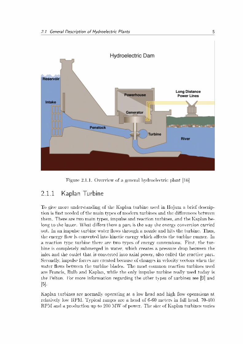
As stated in Section 1.1 hydroelectric plants work on the principle of convertingthe potential energy between two water levels, �rst into mechanical power and laterinto electrical power. Below in 2.1.1 the main components of a plant are shown.The basic principle is that water �ows from a reservoir or river through a penstockand powers a turbine which creates a mechanical torque and rotational speed whichgenerates electrical power from a generator. Gross power, Pgross [W], generated bythe plant is dependent on the discharge Q [m3/s] and the gross water head Hgross
[m] according to [9]Pgross = ρQgHgrossη. (2.1.1)
In Equation 2.1.1 ρ is the density of water and η is the turbine e�ciency . Thegross head Hgross in a plant is de�ned as the height between the water level of thereservoir and water level of the outlet destination, in Figure 2.1.1 this would bereservoir level minus the water level of the river. There is also a net head:
Hn = Hgross −HL, (2.1.2)
where HL is the sum of all the losses in head throughout the system due to friction,turbulence and so forth. The net power Pn [W] acting on the turbine then becomes
Pn = ρQgHnη, (2.1.3)
4
2.1 General Description of Hydroelectric Plants 5
Figure 2.1.1. Overview of a general hydroelectric plant [16]
2.1.1 Kaplan Turbine
To give more understanding of the Kaplan turbine used in Hojum a brief descrip-tion is �rst needed of the main types of modern turbines and the di�erences betweenthem. There are two main types, impulse and reaction turbines, and the Kaplan be-long to the latter. What di�ers them a part is the way the energy conversion carriedout. In an impulse turbine water �ows through a nozzle and hits the turbine. Thus,the energy �ow is converted into kinetic energy which a�ects the turbine runner. Ina reaction type turbine there are two types of energy conversions. First, the tur-bine is completely submerged in water, which creates a pressure drop between theinlet and the outlet that is converted into axial power, also called the reactive part.Secondly, impulse forces are created because of changes in velocity vectors when thewater �ows between the turbine blades. The most common reaction turbines usedare Francis, Bulb and Kaplan, while the only impulse turbine really used today isthe Pelton. For more information regarding the other types of turbines see [9] and[5].
Kaplan turbines are normally operating at a low head and high �ow operations atrelatively low RPM. Typical ranges are a head of 6-60 meters in fall head, 70-400RPM and a production up to 200 MW of power. The size of Kaplan turbines varies

2.1 General Description of Hydroelectric Plants 6
from two to eight meters in diameter and has four to eight runner blades.
A physical description of the Kaplan is given in Figure 2.1.2 below. A turbinerunner with blades is attached to a shaft connected to the generator. Water entersthe turbine via a spiral cone surrounding the turbine. The wicket gate is acting as avalve and controls the direction and size of the �ow discharges Q [m3/s] by adjustingthe horizontal blades. When the waters has entered the inner parts of the turbinethe vertical angle of the runner blades can be adjusted to deliver the maximumlevel of e�ciency. These adjustable runner blades is the main di�erence betweenthe Kaplan and other types of reaction turbines. Angles for the optimal e�ciencywhen having a certain discharge are determined through experimental testing.
Figure 2.1.2. Kaplan Turbine[16]. Note that Wicked gate should be Wicket gate.
The mechanical power delivered by a turbine can be described as
Pm = Q∆pη = ωTm [W ], (2.1.4)
where ∆p [Pa] is the pressure di�erence between inlet and outlet, η is the turbine ef-�ciency, ω[rad/s] is the rotational speed and Tm [Nm] is the mechanical torque. Thisequation is essentially the same as Equation (2.1.3) expressed in di�erent entities,∆p being interchangeable with ρgHn [9].
2.1 General Description of Hydroelectric Plants 7
2.1.2 Reservoirs, penstocks and outtake
A hydroelectric plant is usually located in the downstream of a body of �owingwater, such as a river. A reservoir is not necessary but often constructed to createa bu�er of energy, thus eliminating the dependency of a steady �ow. The waterconduit between the turbine and reservoir is called a penstock. It can vary in lengthfrom 20 to several thousands of meters and be in the form of open canals, tunnels,pipes or combinations and be constructed in several di�erent materials such as wood,concrete or steel. The penstock is responsible for the major part of a hydroelectricplant system's dynamics.
When opening and closing the wicket gate it takes time for the body of water inthe penstock to accelerate or decelerate and this may create pressure hammers orlag time in the system. Water elasticity may also have to be taken into account ifthe penstock is large enough. Depending on the design and material the penstockcreates a loss in head due to friction and turbulence in the water. The connectionbetween the reservoir and penstock is called a water intake, must be taken intoconsideration since it is a major source of turbulence and friction. The reason forthis is mostly because of its design which often includes edges and a trash rack [5].
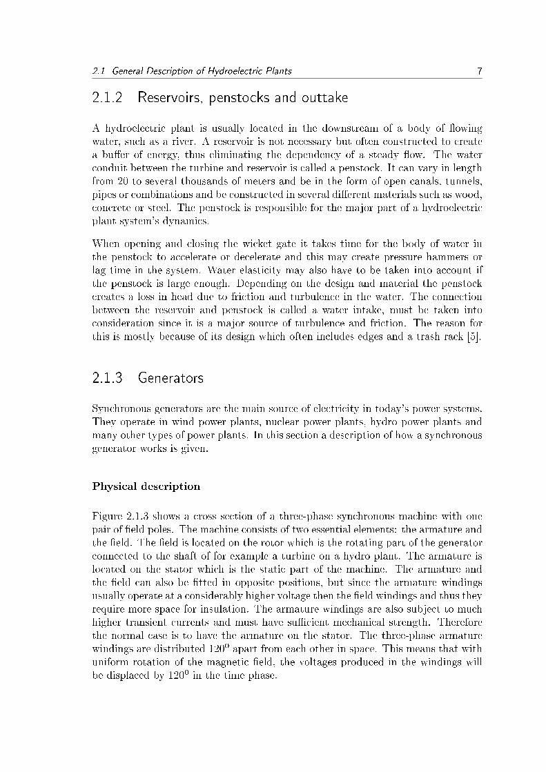
2.1.3 Generators
Synchronous generators are the main source of electricity in today's power systems.They operate in wind power plants, nuclear power plants, hydro power plants andmany other types of power plants. In this section a description of how a synchronousgenerator works is given.
Physical description
Figure 2.1.3 shows a cross section of a three-phase synchronous machine with onepair of �eld poles. The machine consists of two essential elements: the armature andthe �eld. The �eld is located on the rotor which is the rotating part of the generatorconnected to the shaft of for example a turbine on a hydro plant. The armature islocated on the stator which is the static part of the machine. The armature andthe �eld can also be �tted in opposite positions, but since the armature windingsusually operate at a considerably higher voltage then the �eld windings and thus theyrequire more space for insulation. The armature windings are also subject to muchhigher transient currents and must have su�cient mechanical strength. Thereforethe normal case is to have the armature on the stator. The three-phase armaturewindings are distributed 120º apart from each other in space. This means that withuniform rotation of the magnetic �eld, the voltages produced in the windings willbe displaced by 120º in the time phase.

2.1 General Description of Hydroelectric Plants 8
Figure 2.1.3. Schematic diagram over a three phase synchronous machine.
A direct current goes through the �eld windings and induces a magnetic �eld φrwhich induces alternative voltage(emf) Er in the armature windings when rotating.This emf is 90º after the induced magnetic �eld φr (see Figure 2.1.4). The armaturecurrent Ia also induces a magnetic �eld φs, which has the same phase location as Ia.An equivalent circuit of one phase in the generator can be seen in Figure 2.1.5.
Figure 2.1.4. Phasor diagram.Figure 2.1.5. Equivalent circuit forone phase.
The �eld winding rotates with the rotor and in order to get a steady torque the �eldsof stator and rotor must rotate at the same speed. This speed is called synchronousspeed. And is given by
n =120f
Pf, (2.1.5)
where n is the speed in rpm, Pf is the number of �led poles in the stator and f isthe frequency in Hz.

2.1 General Description of Hydroelectric Plants 9
2.1.4 Strong grid and Island grid
The generator will be operating in two di�erent settings, strong grid and islandgrid. Strong grid means that the generator is connected to a very big network, forexample the entire network of Sweden, including many generators. Because of thisthe generator will not in�uence the frequency and the voltage of the strong grid.The generator will instead follow the strong grid's frequency and voltage. The poweroutput from the generator to a strong grid can be set to a desired value. Island gridmeans that the generator is alone on the grid and thereby sets the frequency andvoltage on the grid itself. This means that when a load change happens on theisland grid it will e�ect the generator frequency and voltage. On the island grid thepower output from the generator will be equal to what the island grid demands.
2.1.5 Governing a hydroelectric plant
The control system is a vital part of a hydroelectric plant. It is used for controllingand adjusting the total power output and leveling out �uctuations between the gridand plant with respect to power and frequency. A. Kjolle [9] describes this byexpressing two major purposes for turbine governors:
1. �To keep the rotational speed stable and constant of the turbine-generator atany grid load and prevailing conditions in the water conduit�
2. �At load rejections or emergency stops the turbine admission have to be closeddown according to acceptable limits of the rotational speed rise of the unitand the pressure rise in the water conduit.�
In a plant with a Kaplan turbine these goals are achieved by controlling the closingand opening rate of the turbine wicket gate. Thus, controlling the water level in thereservoir to maintain desired head. Note that the adjustable runner blades in theKaplan turbine can used to directly control the plant but in this case are there toachieve maximum e�ciency. In Figure 2.1.6 a general schematic of a typical controlsystem is shown.

2.1 General Description of Hydroelectric Plants 10
Figure 2.1.6. Generic control system in a hydroelectric plant
As can be seen above in Figure 2.1.6 the governor responds to the error between thereference and the current output from the generator. The set point and feedbackdoes not have to be the frequency, it can also be power or load output. A typicalstep response of a governor and a plant when a load reduction is carried out can beseen below in Figure 2.1.7. The dynamics of the plant are such that when there isa load reduction the rotational speed or frequency will increase due to the decreaseof power demanded on the grid (see Figure 2.1.5). A governor will then react to theerror between the reference and feed back and thus closing the wicket gate until thedeviation is eliminated. If a load increase is performed the opposite will occur, i.e.a decrease in rotational speed and an increase in torque.
Figure 2.1.7. Description of a system response when a load reduction is per-formed [9]

2.2 Overview of Modeled System 11
2.2 Overview of Modeled System
This section concerns the system modeled. First a brief description of the Hojumhydroelectric plant in Trollhättan, which is the basis of design for the test benchmodel, followed by an overview of the parts being modeled.
2.2.1 Hojum, Trollhättan
The Hojum plant consist of three power units; G14, G15 and G16, all Kaplan typeturbines. The �rst two was put into operation 1942 and G16 during 1992. In 2008the G15 unit was renovated and both turbine and generator were replaced. Thesystem modeled is based on the design and values from of the G15-unit to thelargest extent possible. Below, in Figure 2.2.1, and a Table 2.1 a schematic andtable with rated values can be seen [15].
Figure 2.2.1. The Hojum G15 unit [14]
Turbine Kaplan with 6 runner bladesDiameter 5.3 m
Rated Head 31 mMaximum Discharge 221 m3/s
Maximum Measured Power Output at 31m head 58 MWRated Generator Power 66 MW
Rated Speed 136.4 rpm
Table 2.1. Rated values of Hojum G15 [14].

2.3 Process Modeling 12
2.2.2 Modeled System
The concept drawing of the system below (see Figure 2.2.2), together with Figure1.1 gives an overview of the system that is modeled and the parts involved. As canbe seen the plant is divided into two main parts regarding the physical modeling; aprocess and an electrical part. The two sub-systems are connected via a governorand transfer of entities between the models.
Figure 2.2.2. Sketch of modeled system.
2.3 Process Modeling
Here follows the modeling of the process part of the plant. The modeling has beendivided into the following independent sub-models of the plant:
� Reservoir and Outtake Reservoir
� The penstock and outtake
� Wicket Gate
� Kaplan Turbine
All of the sub-models have two things in common. The �rst is the principle of massconservation. Mass conservation can be expressed as
dM
dt= min − mout, (2.3.1)

2.3 Process Modeling 13
whereM [kg]is the total mass contained in the volume and min[kg/s] and mout[kg/s],respectively, are the mass �ow rates. Second is a given pressure drop pdrop [Pa] atany time in the model, which is a function of the �ow pdrop = f(Q) [4, 1].
2.3.1 Reservoir and outtake reservoir
The reservoir is considered to have the form of a basic cylinder with the height h[m], constant diameter D [m] and area A [m] . For a volume with a constant crosssection the water level is given by the volume balance
dh
dt=
1
A(QOutflow −QInflow). (2.3.2)
Bottom pressure pbottom [Pa] is then
pbottom = ρgh. (2.3.3)
The out�ow from the reservoir to a connected penstock is modeled as a pressure lossdue to friction, which can be formulated as [6].
pdrop = Koutflowρ
2v2 (2.3.4)
Where Koutflow is a constant of the friction from the exit of the reservoir and v is thevelocity of the water. The total pressure transferred to the penstock then becomes
pin = pbottom − pdrop (2.3.5)
An outtake reservoir is modeled as a reservoir with a very large diameter, hencedhdt
≈ 0.
2.3.2 Penstock and Outtake
The penstock is a major contributor to the dynamics in a hydroelectric plant. Thedynamics are described with the help of the principle of conservation of momentum[4]
dG
dt= minvin − moutvout + (Ainpin − Aoutpout)− Ff + Aρg4h, (2.3.6)
where
2.3 Process Modeling 14
� G is the momentum in the volume [kgm/s]
� vin/out is the velocity at the inlet and outlet of volume [m/s].
� Ain/outis the area at the inlet and outlet of volume [m2].
� Ff is the friction force [N ].
� 4h is the di�erence in height between inlet and outlet of volume[m].
� min and mout is the change in mass�ow at inlet and outlet. They are calculatednumerically by Dymola in each step of the simulation.
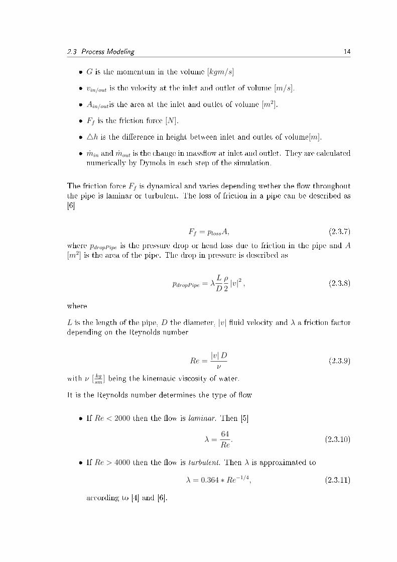
The friction force Ff is dynamical and varies depending wether the �ow throughoutthe pipe is laminar or turbulent. The loss of friction in a pipe can be described as[6]
Ff = plossA, (2.3.7)
where pdropP ipe is the pressure drop or head loss due to friction in the pipe and A[m2] is the area of the pipe. The drop in pressure is described as
pdropP ipe = λL
D
ρ
2|v|2 , (2.3.8)
where
L is the length of the pipe, D the diameter, |v| �uid velocity and λ a friction factordepending on the Reynolds number
Re =|v|Dν
(2.3.9)
with ν [ kgsm
] being the kinematic viscosity of water.
It is the Reynolds number determines the type of �ow
� If Re < 2000 then the �ow is laminar. Then [5]
λ =64
Re. (2.3.10)
� If Re > 4000 then the �ow is turbulent. Then λ is approximated to
λ = 0.364 ∗Re−1/4, (2.3.11)
according to [4] and [6].

2.3 Process Modeling 15
2.3.3 Wicket Gate
The wicket gate is modeled as a valve [1]. A fully opened valve can be expressed as
Q = Kv√pdrop, (2.3.12)
where Kv[m3/h] is how much that �ows through the valve per hour at a speci�c
opening. Kv is dependent on the valve position x that ranges from 0 to 1.
The valve is modeled with �rst order dynamics to represent a lag time when closingand opening the valve:
dx
dt=
1
τ(xinput − xcurrent). (2.3.13)
The time constant τ is the time it takes for the valve to open 63 %.
2.3.4 Kaplan Turbine
The mechanical power from a Kaplan turbine is [9]
Pt = Qpdropηt, (2.3.14)
where Q is the �ow pdrop, is the drop in pressure from turbine inlet to turbine outletand ηt the current turbine e�ciency.
ηt depends on two factors, the �ow through the turbine, and the angle of the runnersblades. The deviation from the maximum e�ciency at a certain �ow is called thecombination error. Data for the combination error is gathered through turbinetesting. Data has been available throughout this project and thus ηt is modeled asa function of the �ow and runner blade angle α i.e.
ηt = f(Q,α) (2.3.15)
or by a look up table
ηt =
α1 α2 · · · αj
Q1 ηt11 ηt12 · · · η1jQ2 ηt21 ηt22 · · · η2j...
......
. . .Qi ηi1 ηi2 ηtij
(2.3.16)

2.4 Electrical Modeling 16
Together with Equation (2.1.4) the mechanical torque Tm [Nm] generated is
Tm =Qpdropηtωs
, (2.3.17)
where ωs[rad/s] is the synchronous speed of the generator.
2.4 Electrical Modeling
This section includes the model equations for a synchronous generator of third order,description of load model and slack model.
2.4.1 Modeling of synchronous generator
Figure 2.4.1. Rotor and stator circuits of a synchronous machine.
2.4.2 The DQ-transformation
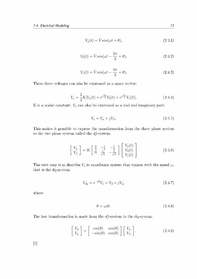
When studying electric machines its preferable to transform the regular three phasesystem to an equivalent two phase rotating coordinate system called the dq-system[7]. d and q are two �ctitious axles perpendicular to each other located on therotor (see Figure 2.4.1) that rotates with the same speed as the magnetic �eld inthe machine. The transformation is made in two steps: 1) A transformation fromthe three-phase stationary coordinate system to a two phase stationary coordinatesystem called the ab-system. 2) A transformation from the ab-system to the dqrotating system. A three phase system consists of the following voltages:
2.4 Electrical Modeling 17
Va(t) = V sin(ωt+ θ), (2.4.1)
Vb(t) = V sin(ωt− 2π
3+ θ), (2.4.2)
Vc(t) = V sin(ωt− 4π
3+ θ), (2.4.3)
These three voltages can also be expressed as a space vector:
Vs =2
3K[Va(t) + ej
2π3 Vb(t) + ej
4π3 Vc(t)], (2.4.4)
K is a scalar constant. Vs can also be expressed as a real and imaginary part:
Vs = Vα + jVβ, (2.4.5)
This makes it possible to express the transformation from the three phase systemto the two phase system called the ab-system.
[VαVβ
]= K
[ 23−1
3−1
3
0 1√3− 1√
3
] Va(t)Vb(t)Vc(t)
(2.4.6)
The next step is to describe Vs in coordinate system that rotates with the speed ω,that is the dq-system:
Vdq = e−jθVs = Vd + jVq, (2.4.7)
where
θ = ωdt. (2.4.8)
The last transformation is made from the ab-system to the dq-system:
[VdVq
]=
[cos(θ) sin(θ)−sin(θ) cos(θ)
] [VαVβ
]. (2.4.9)
[7]

2.4 Electrical Modeling 18
2.4.3 Per-Unit system
All the generator and network models are in per-unit, which means that all thevalues are normalized to a common MVA base. This is standard practice in powersystem analysis and usually the generator parameters are given in per-unit from themanufacturer. By normalizing for example the generator equations it will be easierto understand the generator performance due to that the parameters will be of sametype. The per-unit value is calculated in the following way[11]:
PerUnitvalue =actualvaluebasevalue
(2.4.10)
2.4.4 Third order model of synchronous generator
The transformation from the normal three phase system to the dq-system enablesa model (see Section 2.4.5) to be built were the equations are written in the dqcoordinate system. A model of third order was chosen, and a number of assumptionmust be made for the model to work:
1. The three-phase stator windings are symmetrical.
2. The capacitance of all windings can be neglected.
3. Each of the distributed windings may be represented by a concentrated wind-ing.
4. The change in the inductance of the stator windings due to rotor position issinusoidal and does not contain higher harmonics.
5. Hysteresis loss is negligible but the in�uence of eddy currents can be includedin the model of the damper windings.
6. In the transient and sub-transient states the rotor speed is near synchronousspeed.
7. The magnetic circuits are linear (not saturated) and the inductance values donot depend on the current.
Worth mentioning is that there are higher order generators models. What di�ersbetween the models is how many transient states in the circuits you want to study.In this paper a third order model was chosen to be su�cient, but the model caneasily be expanded to include more transient states. Figure 2.4.2 corresponds to thedi�erent transient states for q and d-axis. The transient states are due to that in thetransient periods the armature �ux is forced to paths outside the �eld windings bycurrents that are induced in the �eld windings, the armature �ux have both d andq-components. The �ux path is distorted by the d-axis �eld current and by q-axis

2.4 Electrical Modeling 19
rotor body currents. Each of the transient EMF's have a time constant which isthe time it takes for the magnetic energy stored in the winding to decay to 0(steadystate) [11].
Figure 2.4.2. Generator equivalent circuits for q and d-axis with resistanceneglected[8].
2.4.5 Model equations
2.4.5.1 Voltage equations
Vd = −raId −XqIq (2.4.11)
Vq = E′
q +X′
dId − raIq, (2.4.12)
where ra is the armature resistance, Xq is the Q-axis synchronous reactance, X′d is
the D-axis transient reactance, E′q is the Q-axis transient emf, Vd is the voltage in
d-axis and Vq is the voltage in q-axis (see Figure2.4.2) [11].
2.4.5.2 Swing equations
The swing equations describe the mechanical behavior of the generator:
ω =1
2H(Pm − Pe −D(ω − 1)), (2.4.13)
δ = 2π50(ω − 1), (2.4.14)
Pe = E′
qIq + (X′
d −Xq)IdIq, (2.4.15)
where ω is the rotor speed, Pm is the mechanical power from the turbine, P e isthe electrical power out from the generator, D is the dampening coe�cient, δ is therotor angle and H is the inertia constant for generator and turbine [11].

2.4 Electrical Modeling 20
2.4.5.3 Transient EMF equations
The transient EMF equation desribes the behavior of the magnetic �ux in the q-axiswinding:
T′
d0E′q = Efd − E
′
q + Id(Xd −X′
d), (2.4.16)
where T′
d0 is the D-axis transient time constant and Efd is the �eld current set bythe voltage controller (see Section 2.5.2) [11].
2.4.5.4 Generator parameters
The following parameters were used in the generator model, which is taken from thedata from G15 Hojum (see Appendix 1.2):
Parameter Value DescriptionSn 66 MW Rated powerUn 11.3 kV Rated voltageXd 1.041 pu D-axis synchronous reactanceXq 0.651 pu Q-axis synchronous reactanceX
′
d 0.3 pu D-axis transient reactanceH 9 Inertia constantD 0 Dampening coe�cientra 0 Armature resistance
Table 2.2. Generator parameters.
2.4.6 Load model
The load model is a constant PQ load which means that the load draws a constantP (active power) and a constant Q (reactive power) from the network. Throughparameters in the model the amount of active and reactive power is set. Also a thirdparameter is connected to the model that makes it possible to change how much ofthe load is used. The interval is set to 0-100% and this parameter is controlled viathe interface in LabVIEW. This makes it possible to make load changes in real timeand see how the generator reacts.
2.4.7 Slack model
The slack model is used to imitate the behavior of a strong network, e.g. the wholepower grid of Sweden. The Slack node can be seen as a generator with constant

2.5 Control Theory 21
voltage and constant frequency and when this node is connected to the grid it actsas a reference to other generators on the grid. The Slack model is connected to thegrid when the model is running on a strong grid.
2.5 Control Theory
In this section the control theory of the hydro power plant will be described. Thereare three control loops that controls the power plant:
� Frequency control that controls the rotor speed in the generator and hence thefrequency of the grid.
� Voltage control that controls the �eld current in the generators rotor whicha�ects the voltage output from the generator.
� Water level control that controls the water level in the reservoir through damhatches.
The type of controller that are used for these control applications are PID controller.PID stands for proportional-integral-derivative and is a widely used controller inindustrial control systems. A PID controller calculates an error between the set-point value r(t) (the preferred value in the process) and the process value y(t) (theactual value of the process) (see Figure 2.5.1). The controller then tries to minimizethe error through a control algorithm that contains the three parts P, I and D. TheP part depends on the present error, I part accumulates past errors and D dependson the rate of changes in the error. The sum of these three values then becomesthe control signal u(t) that adjusts the process so that eventually, with the rightparameter values, the error e(t) converges to 0.
Figure 2.5.1. Block diagram over PID controller[9].

2.5 Control Theory 22
2.5.1 Frequency control
The frequency of the generator depends on the rotor speed. To get the right fre-quency the generator must rotate at synchronous speed. The speed of the generatordepends on the water �ow through the turbine. Hence, to be able to control thespeed of the generator the water �ow through the turbine is controlled by a hatch.The input to the generator model is the mechanical power of the turbine Pm (seeEquation (2.4.13)) that depends on the �ow.
The frequency controller is a PID controller, the set-point value r(t) constitutes ofthe preferred frequency and the measured value y(t) is the actual frequency. Throughthe error e(t) a control signal u(t) is calculated that controls the valve position ofthe wicket-gate (see Section 2.3.3). The wicket-gate controls the water �ow into theturbine. The control signal is constrained the values between 0 and 1, which meansthat at 0 the hatch is closed and at 1 the hatch is completely open.
2.5.2 Voltage control
The output voltage from the generator is controlled by the �eld current in the rotorwindings and is controlled by an PID controller. The set-point r(t) is the preferredvoltage output and the process value y(t) is the measured voltage on the stator.The output from the controller is the �eld current for the stator-winding Efd.
2.5.3 Reservoir Level Control
In smaller reservoirs it is possible to control the water level via extra dam hatchesso that water is by-passed the turbine and power unit. The set-point r(t) becomesthe preferred water level and the process value y(t) is the measured water level. Thecontrol signal u(t) controls the extra dam hatches to get the preferred water levelin the reservoir.

3 IMPLEMENTATION
This chapter concerns the implementation part of the modeling in Chapter 2. Itbegins with a description of the tools that have been used and then follows the im-plementation of the physical model, construction of GUI, design of control sequencesand how to establish communication.
3.1 Software and Communication Protocols
Below follows a short descriptions of the various software and communication pro-tocols used.
3.1.1 Dymola
All the models are made in Dymola which is an object oriented graphical simulationprogram that uses the simulation language Modelica. Dymola is an equation-basedsimulation tool unlike block-oriented tools such as Simulink. In Dymola you canboth use graphical code and also manually entered row-based code. If graphicalcode is used Dymola will convert all the graphical code into Modelica code beforesimulation. The simulation environment is divided into two parts: the modelingpart and the simulation part. The modeling part is where you draw the models andcheck them regarding to syntax and structure. In the simulation part the code is�rst converted into C-code and then simulated. In the simulation editor it is possibleto look at plots of all variables in the model. An example of a model in Dymolais showed in Figure 3.1.1 where a graphical view of the model is showed in the leftwindow and the simulation tool is showed in the right window [2].
Figure 3.1.1. Modeling window(left side) and Simulation window(right side).
23

3.1 Software and Communication Protocols 24
3.1.2 LabVIEW
LabVIEW 8.2 has been used to create the graphical user interface (GUI) and forimplementation of the control sequences.
LabVIEW is a software programming tool developed by National Instrument. It usesa high level graphical programming language which resembles �ow charts. Programsare executed by the way graphical blocks in a program are connected. A programin LabVIEW is called a VI or virtual instrument and contains an interface view anda graphical programming view. The user can create standard and custom graphicalcomponents in the interface view and connect them in the programming view, thusenabling a relatively simple and fast way to design a GUI. The LabVIEW standardlibrary is extensive and has a lot of modules for network support, such as the OPCprotocol.
3.1.3 TOP Server
Top Server is an OPC Server and HMI (human machine interface) connectivitydeveloped by Software Toolbox, North Carolina, USA. It works as a native OPCserver which is a bridge to multiple non-OPC communication protocols, such asDDE (see below). This means that you can establish communication between twoplatforms that uses two di�erent protocols.
3.1.4 Communication Protocols
OPC
OPC stood for OLE (Object Linking and Embedding) for Process Control but isnow to be associated with �open connectivity via open standards�. It was developedby an industry collaborative task force in 1996, and the goal was to create a standardwithin industry automation. Later the OPC Foundation was founded and took overthe responsibilities of further developing and maintaining the standard. For furtherand more detailed information regarding the OPC standard and the OPC foundationvisit www.opcfoundation.org.
DDE
Dynamic Data Exchange (DDE) is a protocol to enable data transfer across Win-dows based programs using the native messaging function between applications inWindows. It is an old technology that has been phased out by newer technologiessuch as netDDE but is still used today in various applications, such as Dymola. Theapplication that sends data through DDE acts as an DDE-server.

3.2 Physical Model 25
3.2 Physical Model
The physical model of the hydroelectric plant is modeled in Dymola using compo-nents in Chapter 2. It is divided into an electrical part and a process part of theplant. In Figure 3.2.1 below an overview of the implemented model can be seen.Since Dymola is object oriented all the separate sub-models and systems have beendeveloped as independent classes. Thus it is relatively easy to create new scenariosand variations of the physical model. Classes in the model are connected to eachother through a basic Dymola class called Connector. A connector is able to workas a communication port and transfer entities from one model to another.
Figure 3.2.1. Graphical overview of the model implemented in Dymola
The standard library in Dymola has been used to the largest extent possible for theproject, this including mathematical operations, values of constants and so forth.External inputs are done by having constant signals connected to an inport in aDymola model. Out ports can be read externally directly.
3.2.1 Process
The process part of the model is implemented in Dymola with the components in thelist below. Connectors in the process part are called �ow ports and carry information

3.2 Physical Model 26
about pressure and mass �ow rate through connected parts in the system.
� Reservoir. Works both as the dam reservoir and out�ow area. Calculations ofbottom pressure, water level and friction losses due to the outlet and inlet arecalculated in this class. A reservoir has one �ow connector for water �owingin to or out of to the reservoir. The dam reservoir is an altered version of thebasic reservoir such that it has extra connectors for additional out�ow due tolevel control dam hatches and additional in�ow.
� Penstock. The penstock is where water friction losses and momentum balanceare calculated. Main parameters are length, diameter and it uses two �owconnectors.
� Wicket Gate. Used to simulate the guided vanes in the plant. It has a inputport which range from a value of 0 to 1 and an outport which gives the currentposition of the gate. Depending on the input, pressure loss and �ow through-put are calculated. A Wicket Gate class with di�erent input parameters isused to simulate the emergency dam hatches.
� Kaplan Turbine. Contains the Wicket Gate model. It has several inports andoutports, the in ports are wicket gate input, actual head for calculation ofe�ciency and rotational speed determined by the generator. The outports aree�ciency, runner blade and wicked gate angle, �ow in turbine and �nally themechanical torque generated which is connected to the generator. Calculationsperformed in the class are the �ow throughout the turbine, mechanical powergenerated, losses due to friction, angle of runner blades and correspondinge�ciency factor.
3.2.2 Electrical
The electrical part of the Dymola model consists of a generator of 3rd order, a Slacknode and a load. The model is made so that it can either be run in an island network,where only the generator is connected to the load, or in strong network where boththe generator and the load are connected to a Slack node that acts as a voltageand frequency reference. Included in the model is also the voltage controller for thegenerator that controls the �eld current in the generator. The electrical model inputsare Pm, Loadstep and BreakerSignal see Figure 3.2.2. Pm is the mechanical powerfrom the turbine that drives the generator model (see Equation(2.4.13)). Loadstepis a parameter that is set in LabVIEW and determins how much of the load thatused. BreakerSignal closes and opens the breaker. The outputs from the model areV, Pe, and w. V is the phase voltage of the generator, Pe is the electrical power thatthe generator produces to the network and w is the rotational speed of the generator,which also decides the frequency. w is also fed back to the turbine model becausethe generator shaft is connected to the turbine and runs on the same rotationalspeed. The slack node is connected via a breaker that makes it possible to connect
3.3 Interface and Control Sequences 27
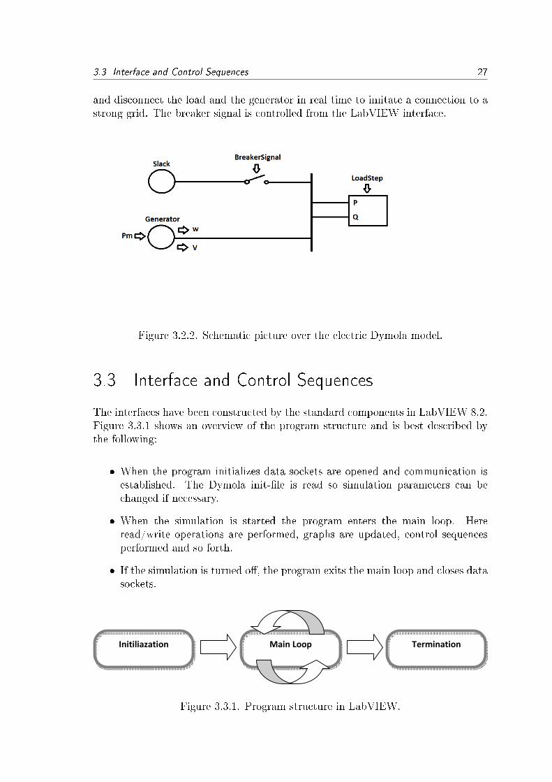
and disconnect the load and the generator in real time to imitate a connection to astrong grid. The breaker signal is controlled from the LabVIEW interface.
Figure 3.2.2. Schematic picture over the electric Dymola model.
3.3 Interface and Control Sequences
The interfaces have been constructed by the standard components in LabVIEW 8.2.Figure 3.3.1 shows an overview of the program structure and is best described bythe following:
� When the program initializes data sockets are opened and communication isestablished. The Dymola init-�le is read so simulation parameters can bechanged if necessary.
� When the simulation is started the program enters the main loop. Hereread/write operations are performed, graphs are updated, control sequencesperformed and so forth.
� If the simulation is turned o�, the program exits the main loop and closes datasockets.
�
���������������������� ����������
Figure 3.3.1. Program structure in LabVIEW.

3.3 Interface and Control Sequences 28
Figure 3.3.2 below shows an extract from the implemented program in the LabVIEWblock view.
Figure 3.3.2. Extract from the block view in LabVIEW to demonstrate how theimplementation looks like.
There are no control theory components, such as PID controllers, included in the 8.2standard library. However National Instrument developer zone have demos availablefree of use demonstrating how to implement generic PID controllers with the compo-nents available. The controllers in this project are based on designs in these demos,however they are altered to �t this projects speci�c needs. Figure 3.3.3 below showsan example of a PI controller used for level control in LabVIEW.

3.4 Communication 29
Figure 3.3.3. Implementation of a PI type controller in LabVIEW.
3.4 Communication
To establish communication between the model in Dymola and the interface inLabVIEW, TOP Server is used. The general principle for connecting the programscan be seen in Figure 3.4.1 below.
�
�����������
������������ ��������
�� ����
����� ���
�����������
�������
�� ������������� ����
Figure 3.4.1. Communication between LabVIEW, TOP Server and Dymola.
Dymola has a built in support for DDE communication via Dymosim, which isan executable �le generated when compiling the model. Dymosim has a built inDDE-server and creates tags and addresses based on name of components in themodel.
In LabVIEW the DataSocket component in the standard Library is used. How toestablish read and write functionality between LabVIEW and an OPC server canbe seen in Figure 3.4.2.

3.4 Communication 30
Figure 3.4.2. How to write and read from OPC addresses using the built in datasockets in LabVIEW.
Appropriate sampling rates in the system are decided through testing and tuning.

4 SIMULATION AND RESULTS
4.1 Validation and Veri�cation
Below follows a description of how the veri�cation and validation is performed andthe result of it. Note that in the graphs taken from LabVIEW, the X-axis is notreal time but number of samples in LabVIEW. One sample equals 0.02 seconds.
4.1.1 Veri�cation
The veri�cation of the model and interface is done by testing di�erent scenarios andinvestigate if they respond as desired. The procedure took place in the followingway:
� Test of model and sub-models in Dymola. Besides standard compilation inDymola of the components each one was tested individually by setting updi�erent test scenario and then examining that desired entities are transferredthrough the system. For example one test consisted of two reservoirs connectedwith a pipe. It was examined if �ow and pressure was transferred through thesystem and that the water levels leveled out. Similar tests were conducted onall components in the system.
� LabVIEW program. In LabVIEW the veri�cation procedure was to run theprogram and see that the interface compiled and the controls gave the correctresults.
� Communication. The veri�cation of the communication between LabVIEWand Dymola was done in TOP Server. Signals were sent from LabVIEW andit was veri�ed in TOP Server that the Dymola model registered them.
The �nal physical model passed all the above steps of veri�cation.
4.1.2 Validation
There are three stages of validation. In the �rst, the test bench is compared toexisting theory regarding hydroelectric plants and similar works, in the the secondthe output is compared to data obtained from the Hojum plant [14] and the thirdis a comparison of the output against another simulation software, Simpow.
31
4.1 Validation and Veri�cation 32
Validation against theory
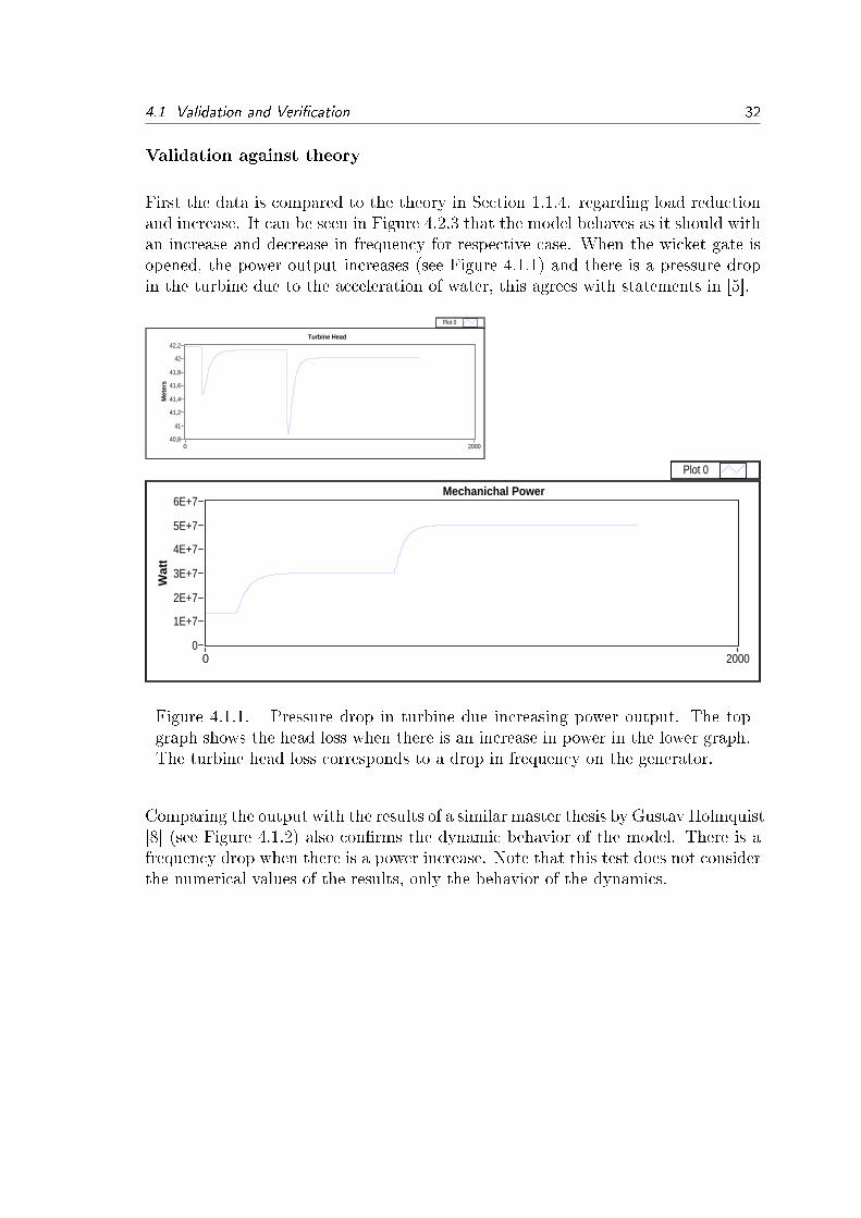
First the data is compared to the theory in Section 1.1.4. regarding load reductionand increase. It can be seen in Figure 4.2.3 that the model behaves as it should withan increase and decrease in frequency for respective case. When the wicket gate isopened, the power output increases (see Figure 4.1.1) and there is a pressure dropin the turbine due to the acceleration of water, this agrees with statements in [5].
Met
ers
42,2
40,8
41
41,2
41,4
41,6
41,8
42
20000
Plot 0
Turbine Head
Wat
t
6E+7
0
1E+7
2E+7
3E+7
4E+7
5E+7
20000
Plot 0
Mechanichal Power
Figure 4.1.1. Pressure drop in turbine due increasing power output. The topgraph shows the head loss when there is an increase in power in the lower graph.The turbine head loss corresponds to a drop in frequency on the generator.
Comparing the output with the results of a similar master thesis by Gustav Holmquist[8] (see Figure 4.1.2) also con�rms the dynamic behavior of the model. There is afrequency drop when there is a power increase. Note that this test does not considerthe numerical values of the results, only the behavior of the dynamics.

4.1 Validation and Veri�cation 33
Figure 4.1.2. Similar dynamic behavior in frequency drop was achieved inanother master thesis by Gustav Holmquist [8].
Validation against Hojum
A test versus data obtained from [15] was performed. In the test the power outputdata from Hojum was used as a reference for the plant. Flow data from Hojumwas then compared with the �ow in the model. The result is shown in Table 4.1below. Note that the model is subject to tweaking and tuning of input parametersand therefore it is easy to change the output of the model in either direction. In thistest, parameters were tuned from raw turbine -and generator data obtained fromHojum [15], however there was no intensive tuning of the system.

4.1 Validation and Veri�cation 34
PHojum[MW ] QHojum[m3/s] QModel[m3/s] Error
13.818 53.84 50.3 -7 %21.324 79,556 78.2 -1,7%31.404 114.978 112.7 -2%41.233 149.659 148.5 -0.7%51.776 192.094 194.5 1.1%55.549 204.687 211 3%58.642 215.362 228.01 5.8%
Table 4.1. Test of output power versus �ow for Hojum and the model at a headof 31 meters. [15]
To test the system dynamics towards the real plant in Hojum real operational datawas obtained (see Appendix A.2). However due to technical di�culties during thegathering of the data these are deemed insu�cient for a satisfying validation (seeSection 5.1.1). They were however compared visually with the output of the testbench and indicated similar behaviour.
Validation against Simpow
To be able to validate the behavior of the model, a model in Simpow was made.Simpow is an electric simulation program with veri�ed models that ÅF uses inelectric system simulations. The model in Simpow consists of a generator with thesame parameters as the one used in the Dymola model, connected to a constant PQload with the same load parameters as the one in Dymola. Both the generator inthe Dymola simulation and the Simpow simulation had a base production at 13.2MW when an increase of 0.66 MW of the load was made. The result from theSimpow model was then compared with the Dymola model (see Figure 4.1.3 andFigure 4.1.4).
% o
f set
poi
nt fr
eque
ncy
and
rate
d R
PM
100,05
99,7
99,75
99,8
99,85
99,9
99,95
100
time(s)20000 200 400 600 800 1000 1200 1400 1600 1800
Omega
Figure 4.1.3. Frequency behavior of Dymola model. Note that X-axis is not realtime but the number of samples in LabVIEW.

4.2 Results 35
Figure 4.1.4. Frequency behavior of Simpow model.
4.2 Results
4.2.1 Interface
The interface that was built in LabVIEW had two objectives, it should give a goodpicture over the hydro-power plant and give information of the essential parametersof the process. The controllers for frequency, power output and water level controlshould be built in LabVIEW and control the Dymola model. The controllers werebuilt in LabVIEW because it makes it possible to make changes to the controllerparameters in real time while running the model. In this section a description of theinterface will be made. The interface consists of two main parts, the control panelwhich controls the process model in Dymola and the process overview where graphsover all the essential parameter can be observed.
Control panel
The control panel in LabVIEW (see Figure 4.2.1) has a number of di�erent param-eters that in�uences the behavior of the model. It includes the three controllers:
1. Frequency controller seen in the upper left corner. Here the three PID param-eters can be set and the frequency set point.
2. Power output controller seen in the middle left. This controller controls thedesired power output from the generator when it is connected to a strong grid.Also here the three PID parameters can be set and the power output set point.
3. Water level control seen to the right of the power output control. Here thePI parameters can be set and the reservoir water level set point. Two more
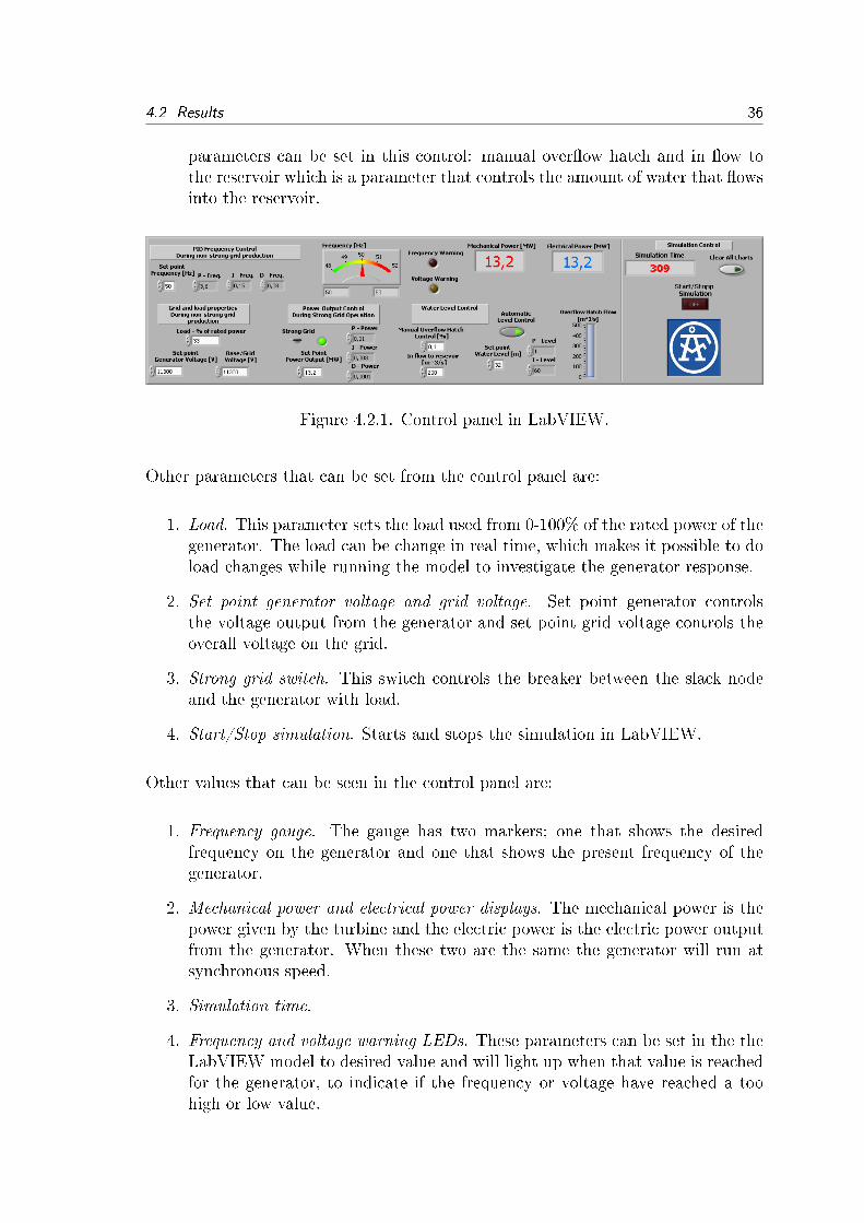
4.2 Results 36
parameters can be set in this control: manual over�ow hatch and in �ow tothe reservoir which is a parameter that controls the amount of water that �owsinto the reservoir.
Figure 4.2.1. Control panel in LabVIEW.
Other parameters that can be set from the control panel are:
1. Load. This parameter sets the load used from 0-100% of the rated power of thegenerator. The load can be change in real time, which makes it possible to doload changes while running the model to investigate the generator response.
2. Set point generator voltage and grid voltage. Set point generator controlsthe voltage output from the generator and set point grid voltage controls theoverall voltage on the grid.
3. Strong grid switch. This switch controls the breaker between the slack nodeand the generator with load.
4. Start/Stop simulation. Starts and stops the simulation in LabVIEW.
Other values that can be seen in the control panel are:
1. Frequency gauge. The gauge has two markers; one that shows the desiredfrequency on the generator and one that shows the present frequency of thegenerator.
2. Mechanical power and electrical power displays. The mechanical power is thepower given by the turbine and the electric power is the electric power outputfrom the generator. When these two are the same the generator will run atsynchronous speed.
3. Simulation time.
4. Frequency and voltage warning LEDs. These parameters can be set in the theLabVIEW model to desired value and will light up when that value is reachedfor the generator, to indicate if the frequency or voltage have reached a toohigh or low value.

4.2 Results 37
Process overview
Process overview interface consist of three tabs Initialization, Overview and Detailedview (see Figure 4.2.2) explained below:
� Initialization. Di�erent initialization parameters can be set in the Dymolamodel.
� Overview. Consists of a conceptional picture of the hydro-power plant (seeAppendix A.1) where di�erent process values are shown in the picture i.e.water �ow through the turbine, power output etc. This is to get a visualpicture of the di�erent components of the power plant and to get a goodunderstanding of how they in�uence each other.
� Detailed view. Graphs over the process parameter are showed and also apicture over a turbine with turbine parameters integrated. This tab also havefour sub tabs which are sorted in the following way:
� Omega/Mechanical Power/Flow. Omega is the frequency over the gener-ator, Mechanical power is the power that the turbine produces and Flowis the water �ow in the turbine.
� Electric Power/Voltage/E�ciency. Electric Power is the power outputfrom the generator, Voltage is the voltage of the generator and E�ciencyis the e�ciency of the turbine.
� Turbine Head/Blade and Guide Vane Angle. Shows the current angleof the wicket gate guide vane and the runner blade angle in the Kaplanturbine.
� Water Level. Water level of the reservoir.
The two graphs that are always shown in this tab regardless of what sub tabis shown are Control error and Control Signal to guide vane. Control error isthe error from the frequency controller and Control Signal to guide vane is thecontrol signal to the wicket gate.

4.2 Results 38
Figure 4.2.2. Process overview interface.
4.2.2 Frequency control
In Figure 4.2.3 the frequency behavior of the generator is shown after a load step.The generator has a base production of 13.2 MW before the load step. The loadstep is an increase in load of 0.66 MW which is one percent of the generator's ratedpower.
% o
f set
poi
nt fr
eque
ncy
and
rate
d R
PM
100,05
99,7
99,75
99,8
99,85
99,9
99,95
100
time(s)20000 200 400 600 800 1000 1200 1400 1600 1800
Omega
Figure 4.2.3. Generator frequency after a load increase of one percent of ratedpower. Note that X-axis is not real time but the number of samples in LabVIEW.
Another test that was performed was how the model would react to a loss of stronggrid (see Figure 4.2.4). In this simulation the generator is running against a stronggrid with a power output of 50 MW when the strong grid is disconnected. Thegenerator goes from an output of 50 MW on a strong grid to an island grid witha small load of 0.66 MW. This will make the frequency to increase rapidly and thesimulation goal is to see how the regulator handles this problem.

4.2 Results 39
% o
f set
poi
nt fr
eque
ncy
and
rate
d R
PM
120
97,5100
102,5105
107,5110
112,5115
117,5
time(s)79900 500 1000 1500 2000 2500 3000 3500 4000 4500 5000 5500 6000 6500 7000 7500
Omega
Figure 4.2.4. Frequency behavior of the generator when strong grid is discon-nected at an power output of 50 MW. Note that X-axis is not real time but thenumber of samples in LabVIEW.
4.2.3 Voltage Control
Figure 4.2.5 shows the voltage behavior of the generator after an increase in load of3.3 MW. The set point voltage is 11300 V.
Vol
t(V
)
11400
11200
11225
11250
11275
11300
11325
11350
11375
time(s)201414 200 400 600 800 1000 1200 1400 1600 1800
Plot 0
Voltage
Figure 4.2.5. Voltage behavior of generator when increase in load of 3.3 MW.Note that X-axis is not real time but the number of samples in LabVIEW.

5 DISCUSSION
5.1 Results
The general results of the test bench are considered satisfactory. It has been veri�edfunctional in the sense that it can produce a clear output (data from physical model)and responds to user inputs via the GUI. The current version of the test benchhas basic operational control system and operational modes which represents thefunctionality of a real plant in general. The test bench was intended to have a morelogic based control and a detailed safety system with automatic safety proceduresthat takes control of the plant when something goes wrong, but due to lack of timefurther development could not be carried out within this project.
5.1.1 Validation
The dynamics of the test bench validates well in all aspects of operation. It behavesaccording to theory and give similar output to the generator models in Simpow, andthe same dynamics can be seen in a similar master thesis [8]. The model was alsoable to handle a disconnection from strong grid were the frequency did not rise over60 Hz (120% of set point frequency of 50 Hz) which is the industry standard. Thevoltage control also functions in a satisfactory way.
Main issue of concern is the validation results against the Hojum plant. The �ow test(see Table 4.1) gives some indication of the performance of the test bench tuning.However it is not enough since it contains no dynamical features.
When trying to gather real time operational data there was technical di�cultieswith access to the PLC at Hojum. The only data gathered was plots of data withinsu�cient level of detail (see Appendix A.2). There is no way to compare the datawith the output from the test bench other than visually, which is not enough for asatisfying validation. Hence, it is not possible to say if the test bench can be tunedto necessary level of detail to represent the Hojum plant.
5.1.2 Area of use
Due to the lack of validation against a real hydroelectric plant the test bench inits current state is not suitable for use towards any real plant operation. However,since the dynamics of the plant model are veri�ed theorectically the system couldbeused as a demonstrator or educational platform.
40

5.2 Complications 41
5.2 Complications
The main complications during the project were caused by software related issues.Below follows a short description that may be taken into consideration when doingfurther development or similar work:
� The combination of Dymola, TOP Server and LabVIEW is not very stabledue to unknown reasons. A likely cause is the DDE server used in Dymola.
� Dymola version 6.1 was used. This version has no support for the latest Mod-elica libraries, so there is no built in support for complex math or a library for�uid systems. The latest versions of Dymola has this, thus enabling modelingwith more detail and veri�ed components.
� There was no good way of exporting data from graphs in LabVIEW to makeexact comparison with the simulation results from Simpow.
5.3 Future Development
Below follows what is considered to be the most interesting and plausible develop-ment for the test bench.
5.3.1 Development the current physical model
There are many options regarding further development of the model in Dymola.Since the Dymola package is object-oriented it is natural to add components to theplant. This could include other types of turbines, surge tanks, more detailed pipemodels, higher order generators and so forth. Other options are to model hardwareand logic into the physical model to increase the similarities with a real plant. Forexample, safety valves, pressure sensors etc.
5.3.2 Connect physical model to a PLC
By connecting the Dymola model directly to a PLC a more realistic setup is cre-ated that enables testing of real PLC code on Dymola models. This opens up thepossibility of developing, testing, writing and optimizing PLC programs o�-line.

5.3 Future Development 42
5.3.3 Deeper analysis of governor system
A more thorough investigation of a real plants governor can be investigated andimplemented in LabVIEW for example. This includes procedures for emergencyshutdowns, startups, testing and so forth.

6 CONCLUSION
A test bench of a hydroelectric plant has been developed to test the feasibility ofthe concept. The Hojum hydroelectric plant was used as a basis of design. Thetest bech is the result of physical modeling of the plant in Dymola and constructionof an interface and governor in LabVIEW. To connect the interface with the phys-ical model the software TOP Server acted as a socket between the two program'scommunication protocols OPC (LabVIEW) and DDE (Dymola).
The end product is a functional test bench of a hydroelectric plant with graphicaluser interface and governing system. The main features are:
� Graphical overview of the total system.
� Interchangeable design parameters of the plant, for example, length and di-ameter of penstock, size of reservoir, inertia in turbine and generator and lagtime in wicket gate.
� Frequency and Load control during Island Grid Operation.
� Power output control during Strong Grid Operation.
� Water level control.
� Ability to tune controllers in real-time.
Plant dynamics have been validated with good results against theory, generatormodels in Simpow and a similar master thesis. Regarding the Hojum hydroelectricplant a complete validation of the test bench was not possible because data gatheredfrom live operations was not to a satisfactory level of detail.
The concept of developing a test bench for demonstration and educational purposesis considered feasible. The test bench developed is capable of explaining how ahydroelectric plant function and operate. To be able to test di�erent scenarios,new control strategies or operations concerning real plants further development isrequired. The current system may function as a base of development but a lotof work is required, with focus on validating the model against a real plant data,designing a more detailed control system and connecting the test bench to a realPLC system.
43

7 Literature and References
[1] Brezovec M., Kuzle I., Tomisa T. (2006) Nonlinear Digital Simulation Modelof Hydroelectric Power Unit With Kaplan Turbine, IEEE transactions on energyconversion, VOL. 21, NO. 1, march 2006, pp. 256
[2] Dynasim (2006). Dymola Version 6.0. Dynasim AB, Lund, Sweden. http://www.dynasim.se/(Access: 2011-09-14).
[3] E, De Jaeger N. Janssens B. Mal�iet F. Van De Meulebroeke (1994). HydroTrubine Mobel For System Dynamic Studies. IEEE Transactions on Power Systems,Vol. 9, No. 4, November 1994, Belgium.
[4] Elmqvist, H., Tummescheit H., and Otter M. (2003). Object-Oriented Modelingof Thermo-Fluid Systems. Proceedings of 3rd Int. Modelica Conference, Linköping,Sweden, ed. P. Fritzson, pp. 269-286.
[5] European Small Hydropower Association, European Commision (1997). Lay-man's Guidebook on how to develop a small hydro site.http://www.seai.ie/Renewables/Hydro_Energy/EU_layman's_guide_to_small_hydro.pdf(Access: 2011-09-14).
[6] Fabricius S.M.O., Badreddin E. (2002). Modelica Library for Hybrid Simulationof Mass Flow in Process Plants. 2nd International Modelica Conference, March18-19 2002, Germany.
[7] Harnefors L, H-P Nee (2000). Control of Variable-Speed Drives, Electrical Ma-chines and Power electronics Deparnment of Electrical Engineering, Royal Instituteof Thechnology, Stockholm, Sweden.
[8] Holmquist Gustav (2005). Konstruktion av Turbinmodel för kaplanturbiner,Chalmers University of Technology, Sweden.
[9] Kjølle Arne (2001). Hydropower in Norway Norwegian University of Science andTechnology, Trondheim, Norway.
[10] Kundur Prabha (1994). Power System Stability and Control, McGraw-Hill Inc,New York.
[11] Machowski Jan, Bialek Janusz, Bumby James (2008). Power System Dynamics:Stability and Control, Second Edition, John Wiley & Sons.
[12] Modelon AB, Hydro Plant Library,http://www.modelon.com/products/modelica-libraries/ (Access: 2011-09-14).
[13] Taylor C.W. Creesap R.Lee (1976) Real-Time Power System Simulation For Au-tomatic Generated Control, IEEE Transactions OII Power Apparatus and Systems,
44
45
Vol. PAS-95, no. 1, January-February 1976. Oregon, USA.
[14] Vattenfall AB. (2011) Våra vattenkraftverk.http://www.vattenfall.se/sv/vara-vattenkraftverk.htm (Access: 2011-09-14).
[15] Vattenfall Power Consultant AB, Lidström D. (2009) Hojum G15 - veri�eringprestandaförändring Prov 2 efter förnyelse.
[16] Wikimedia Commons,http://commons.wikimedia.org/wiki/File:Water_turbine_(en).svg (Access: 2011-09-14)
[17] Wikimedia Commons,http://commons.wikimedia.org/wiki/File:Hydroelectric_dam_without_text.jpg (Ac-cess: 2011-09-14)
[18] Wikimedia Commons,http://commons.wikimedia.org/wiki/File:Pid-feedback-nct-int-correct.png?uselang=sv(Access: 2011-09-15)

A Appendix
A.1 Conceptional picture over the hydro-power plant
Figure A.1.1. System overview.
46

A.2 Gathered data from Hojum, Trollhättan 47
A.2 Gathered data from Hojum, Trollhättan
Olidan, Hojums kraftstationer / Trendutskrifter
\\WINCCHOJUM\WinCC60_Project_HMI_New\HMI_New.mcp
Copyright (c) 1994-2007 by SIEMENS AG / Automation Power Scandinavia AB
8/3/2011 12:05:14 PM
Layout: @CCCurveControlContents.RPL \\WINCCHOJUM\WinCC60_Project_HMI_New\HMI_New.mcp
1 / 1
Time Range: 02.08.2011 12:04:04 - 03.08.2011 12:04:04
12:04:04 16:52:04 21:40:04 02:28:04 07:16:04 12:04:04
Time Axis
-10.0
-3.0
4.0
11.0
18.0
25.0
32.0
39.0
46.0
53.0
60.0
Valu
e A
xis
Figure A.2.1. Power output in MW(red line) blue line unknown.

A.2 Gathered data from Hojum, Trollhättan 48
Olidan, Hojums kraftstationer / Trendutskrifter
\\WINCCHOJUM\WinCC60_Project_HMI_New\HMI_New.mcp
Copyright (c) 1994-2007 by SIEMENS AG / Automation Power Scandinavia AB
8/3/2011 12:17:50 PM
Layout: @CCCurveControlContents.RPL \\WINCCHOJUM\WinCC60_Project_HMI_New\HMI_New.mcp
1 / 1
Time Range: 02.08.2011 23:41:26 - 03.08.2011 05:32:50
23:41:26 00:51:43 02:02:00 03:12:16 04:22:33 05:32:50
Time Axis
-4.0
7.5
18.9
30.4
41.8
53.3
64.7
76.1
87.6
99.0
110.5
G15 Varvtal Sub 1
Figure A.2.2. Rotational speed in % of rated speed.

A.2 Gathered data from Hojum, Trollhättan 49
Olidan, Hojums kraftstationer / Trendutskrifter
\\WINCCHOJUM\WinCC60_Project_HMI_New\HMI_New.mcp
Copyright (c) 1994-2007 by SIEMENS AG / Automation Power Scandinavia AB
8/3/2011 12:21:28 PM
Layout: @CCCurveControlContents.RPL \\WINCCHOJUM\WinCC60_Project_HMI_New\HMI_New.mcp
1 / 1
Time Range: 02.08.2011 12:20:04 - 03.08.2011 12:20:04
12:20:04 17:08:04 21:56:04 02:44:04 07:32:04 12:20:04
Time Axis
0
30
60
90
120
150
180
210
240
270
300
Valu
e A
xis
Figure A.2.3. Flow in turbine [m3/s]
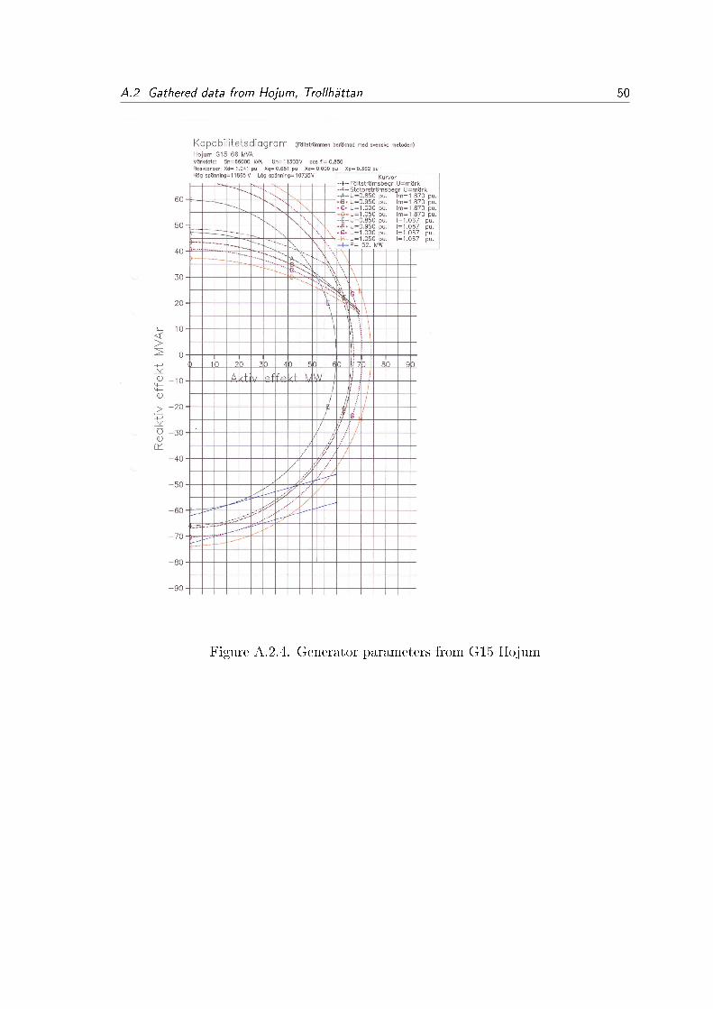
A.2 Gathered data from Hojum, Trollhättan 50
Figure A.2.4. Generator parameters from G15 Hojum