development of a rational methodology for soil
TRANSCRIPT
Development of a Rational Methodology for Soil Geotechnical Characterization
A. Boiero Amundaray Ingeniería Geotécnica, C.A. /Andrés Bello Catholic University, Caracas, Venezuela,
ABSTRACT:The geotechnical characterization of soils is essential for any geotechnical analysis. Such characterization is a complex process that begins during the subsoil exploration, continues with field and laboratory tests and culminates with the interpretation of the available data and the delimitation of sectors of the studied parcel. The development of a rational methodology for geotechnical characterization (RMGC) was based on discriminant analyzes using available data for 1169 soil samples. These analyzes were performed to differentiate the variable soil stiffness. As independent variables, available soil properties in routine geotechnical studies were considered. The validity of the obtained discriminant functions to predict new cases was analyzed, resulting in 81% of new cases correctly classified. A practical application of RMCG in an area of the Araya Peninsula (Venezuela) is presented. Geotechnical zoning and soil behavior drawings were constructed using geostatistical techniques.
Keywords:geotechnical characterization; soil behavior; geomechanical parameters; geostatistics.
1. Introduction Civil Engineering and Environmental Engineering
include the conception, analysis, design, construction, operation and maintenance of a great diversity of struc-tures, facilities and systems, which are built on, in or with soils and/or rocks. In this way, the properties and behavior of these materials have a great influence on the success, economy and safety of the performed work. To properly dealwith the earth materials associated with any project and/or problem, knowledge, understanding, and appreciation of the importance of geology, materials science, materials testing, and mechanics are re-quired[1]. Geotechnical Engineering includes the above, and the subsoil geotechnical characterization is a fun-damental step in this process.
However, it is important to note that uncertainty is an important factor present in the entire geotechnical envi-ronment. Unlike other Civil Engineering disciplines which deals with designed and manufactured materials (such as steel and concrete, for instance), Geotechnics must deal with a wide variety of different materials ori-ginated from complex geological processes, which are normally intermixed and with difficult to determine properties in a precisely way, because they depend on various factors (such as grain-size distribution, minera-logical composition, moisture content, variations in wa-ter table depth, history and stress level, among others). Furthermore, usually the available information is li-mited and imperfectin any geotechnical study[2].
In addition to this uncertainframework, it is worth noting that it is not common in practical Geotechnical Engineering, to carry out rational analysis of available data beyond the application of elementary statistical techniques (basically average and standard deviation), even when over the past five decades significant ad-vances have been made with applications of statistical and probabilistic methods for analyzing soil variability,
as noticed by several authors [2, 3, 4]. This leads to or-dinary geotechnical characterization being supportedby-rough estimates, based on available data and experience in similar geological conditions by the professionals in-volved in a given study.
On the other hand, it is important to emphasize that the rational characterization of the terrain is fundamen-tal for understanding and determine of the subsoil geo-mechanical properties, from which estimates ofsoil strengthand deformations due the action of external loads coming from structures and/or equipment are made. These estimates are directly related to the type of foundations to be implemented in a given project, which in turn is intrinsically associated with costs, schedule and general administration of resources in any engineer-ing work.
Taking into account the above, a rational and practic-al methodology is proposed to characterize thesubsoil, in order to identify in a rational way the presence of po-tentially problematic sectors for the operation of struc-tures and/or equipment. Such methodology is based on the application of geostatistical techniques to field and laboratory data usually available in routine geotechnical studies, and also considers the macroscale soil behavior.
2. Geotechnical characterization For civil engineers, the materials that make up the
earth's crust are arbitrarily classified into two categories: soil and rock.Soil is an accumulation of sediments and other unconsolidated solid particles produced by the mechanical and chemical disintegration of rocks, re-gardless of whether or not they contain an admixture of organic constituents [5]. Rock is a material with a strong internal cohesive and molecular forces which hold its constituent mineral grains together[6].For civil facilities design, understandingsoil behavior is fundamen-tal,sinceitwill experience higher deformations than
rocks under external loads. Thatis why geotechnical characterization is essential for any project.
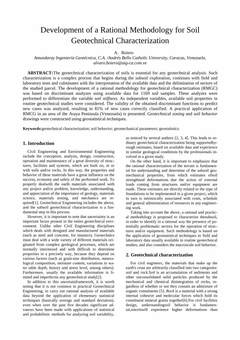
Geotechnical characterization is a complex process that begins during the exploration stage of the subsoil, continues with field and laboratory tests carried out with the purpose of estimating certain properties of the soil, and culminates with the interpretation of the available data and the delimitation of sectors of the studied land, considering the strength characteristics of the detected strata, and the expected response of these strata to ex-ternal loads. Thus, one of the fundamental features of geotechnical characterization includes the zoning of the studied land, in order to identify geologically homoge-neous units, which can coverdifferent geological ages.Fig. 1 schematically shows the geotechnical cha-racterization process.
Figure 1. Geotechnical characterization process.
It must be recognized that a soil strata never are truly homogeneous. The soil properties at a site may show large local variations, yet there may be no general trends to the variations, and the average properties may be es-sentially the same in all portions of the site [7]. This fact is very important, because the analysis of any geotech-nical problem requires the adoption of a soil behavior model, which is based on geotechnical parameters that describe the soil behavior under load-deformation con-ditions. These soil parameters are not known before-hand, so the Geotechnical Engineer must either measure these parameters under controlled laboratory or field conditions, or estimate them from other data [8].In that way, the geotechnical characterization is completed by assigning representative geomechanical parameters toeach sector delimited in the geotechnical zoning. These geomechanical parameters will be used in the geotechnical design of foundations, walls, pavements and earthworks in general, which form part of a project.
3. Soil behavior The texture of soils, especially of coarse-grained
soils, has some relation to their engineering behavior. For fine-grained soils, the presence of water gratley affects their engineering response. Water affects the interaction between mineral grains, and this may affect their plasticity (roughtly defined as the soil´s ability to be molded) and their cohesiveness (its ability to stick togheter). While sands are nonplastic and noncohesive (cohesionless), clays are both plastic and cohesive. Silts
fall between clays and sands: they are fine-grained, yet nonplastic and cohesionless [6].
In general, fine particles fill pore spaces between larger particles, control de permeability of soils, determine whether a given loading condition is drained or undrained, and increase the elastic and degradation thershold strain of soils. Furthemore, a relative small percentage of fines can form stable contacts between coarse grains, providing strength and stiffness to the soil. The Uniform Soil Classification System (USCS) recognizes these observations, clearly separates fines from coarse soils, capture the importance of fines in coarse soils, and even adresses whether those fines are of high or low plasticity [9]. However, it is important to point out that the presence of even a small amount of clay minerals (very small cristaline particles, less than 0.002 mm in size, very active electrochemically) can markedly affect the engineering properties of soil mass. It was recognized that as the amount of clay increases, the behavior of the soil is increasingly governed by the properties of the clay[6, 10, 11]. In that way, as a complement of the information provided by the application of the USCS, understanding the effect of the presence ofclay minerals is fundamental to understanding soil behavior.
At that point, it is important to mention that such soils which behavior is strongly affected by the presence of clay minerals, for simplicity are usually called clays. However, we really mean soils that contain enough clay minerals to affect their engineering behavior. This simplification must be understood, in order to avoid confusion.
The influence of the presence of clay minerals in the soil mass behavior, was extensively studied by several authors in the last four decades. Kenney [12] postulated that residual strength of mixtures of crusshed quartz and different clay minerals, are approximately equal to that the massive mineral when the volume of massive mineral exceeds about 50% of the volume of the mixture. Lupini et al[13] mentioned that residual shear behavior changes significantly as the clay content of cohesive soils increases and a change in a shearing mechanism occurs. Skempton [14] indicated for the clayey soils that if the clay fraction is less than 25%, the soil behaves much like a coarse soil (sand or silt). Georgiannou et al [15] concluded that up to fraction of 20%, clays do not significantly reduce the angle of shearing resistance of the granular component. Pitman et al [16] stated that bellow 20% fines content, sand dominated behavior is observed. Kumar & Wood [17] found that clay matrix govern the mechanical behavior of clay-gravel mixtures when granular fraction is less than 45%. Vallejo & Mawby [18] reported that shear strength of the sand-clay mixtures would be completaly controlled by the sand when fine content is less than 25%. Salgado et al [19] found that fines fully control soil response in terms of dilatancy and shear strength beyond 20% of content. Vallejo [20] indicated that coarser grains control the shear strength of gravel-sand mixtures when finer grain concentration is less than 30%. Biscontin et al [21] stated that coarse grained particles acting as a rigid inclusions in a otherwise clay-water matrix, is a good approximation for fine fractions
higher than 70%; while for very small fractions less than 20% of clay particles, soil behavior is affected only by coarse grains; for 20% to 70% of fine fraction, there is a transition zone, in which the coarse particles are neither in full mutual contact, nor floating in the clay-water matrix.
In order to explain this soil behavior, the two phase model was adopted [10]. According to such model, the void ratio of the granular phase (eg) can be defined as the ratio of volume of the intergranular voids to the volume of granular solids: 𝑒𝑒𝑔𝑔 = 𝑉𝑉𝑣𝑣+𝑉𝑉𝑐𝑐
𝑉𝑉𝑔𝑔 (1)
Where Vv, Vc and Vg are the volume of voids, clay particles and coarse particles (silts, sands or gravels), respectively. Hence, Vv+ Vc is the volume of the intergranular spaces.It is assumed in that model that contribution of fines (clay particles) in sustaining the internal forces is secondary if the amount of fines stays within a certain margin. Instead, the coarser grain matrix is dominant in the transfer of contact friction forces. It is also considered that at relatively low fines content, finer grain matrix in the intergranular void spaces would be highly compressible. The exception case is if the fines are located at the contact points of the coarser grain matrix, or they are trapped in the intergranular void spaces in a compacted manner. There is also the possibility for the fines not being present entirely within the pores of coarser grains, but also be lodged between them even at low fine contents, or might form a thin coating, specially if they are highly plastic [11].
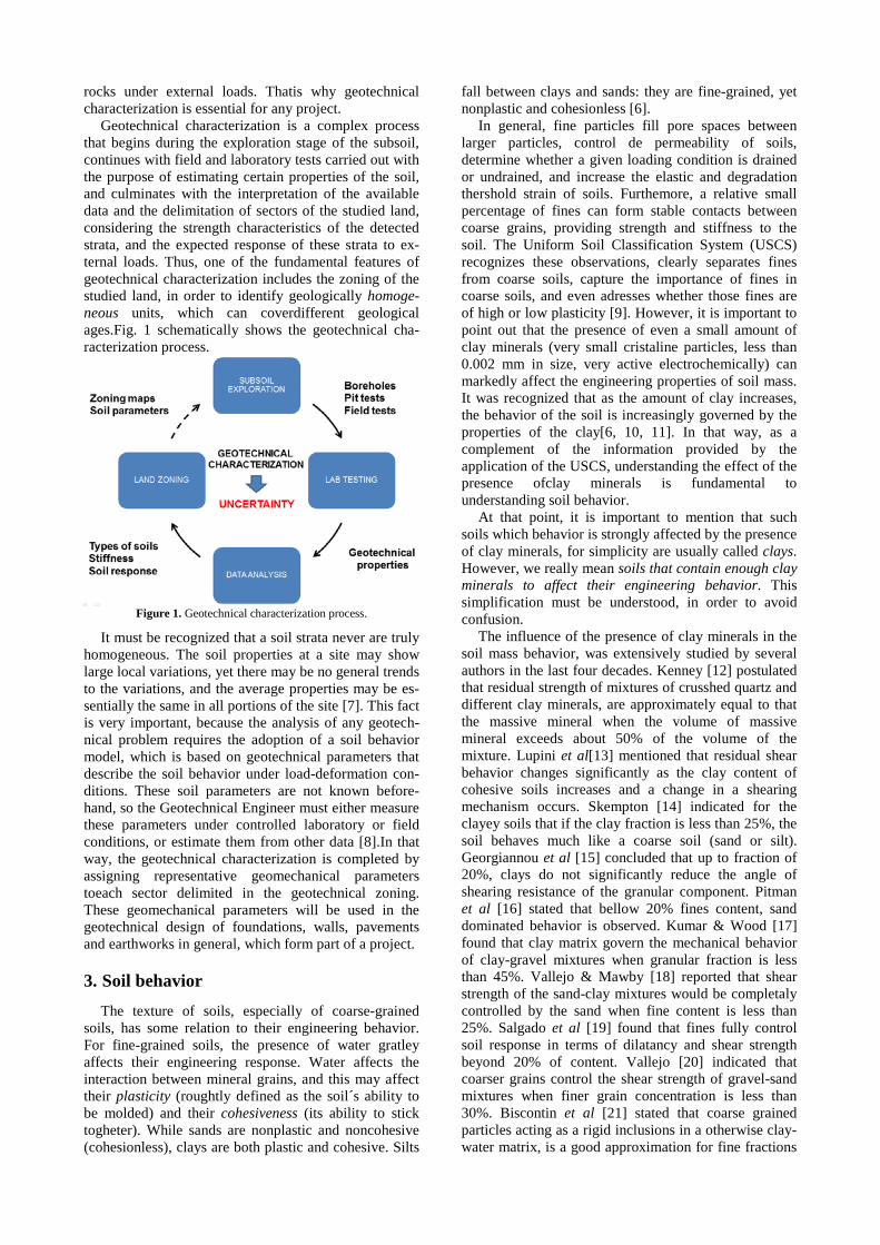
Following the two phase model, saturated soils containing a mix of cohesive and granular soils can be idealized as a combination of the two phases: (1) the clay-water phase, referred as the clay matrix; and (2) the granular phase. Fig. 2 illustrates the model.
Figure 2. Two-phase conceptual model (Source: modified after [21]).
For most practical purposes, Gc ≈ Gg= Gs, and the volumetric clay fraction fc can be approximated by the gravimetric clay fraction FF.The void ratios of the clay-water and granular phases, ec and eg respectivaly, can be determined from the overall void ratio e and the volumetric clay-fraction, according to the following expressions: 𝑒𝑒𝑐𝑐 = 𝑉𝑉𝑤𝑤
𝑉𝑉𝑐𝑐= 𝑒𝑒
𝑓𝑓𝑐𝑐= 𝐺𝐺𝑠𝑠𝜔𝜔
𝐹𝐹𝐹𝐹 (2)
𝑒𝑒𝑔𝑔 = 𝑉𝑉𝑤𝑤+𝑉𝑉𝑐𝑐
𝑉𝑉𝑔𝑔= 𝑒𝑒+𝑓𝑓𝑐𝑐
1−𝑓𝑓𝑐𝑐= 𝑒𝑒+𝐹𝐹𝐹𝐹
1−𝐹𝐹𝐹𝐹= 𝐺𝐺𝑠𝑠𝜔𝜔+𝐹𝐹𝐹𝐹
1−𝐹𝐹𝐹𝐹 (3)
From Eq. (3), if eg ≥ 1, that means that the clay-water phase is greater than the granular phase. In these conditions, the coarser grains behave as rigid inclusions
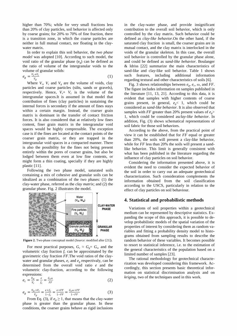
in the clay-water phase, and provide insignificant contribution to the overall soil behavior, which is only controlled by the clay matrix. Such behavior could be defined as clay-like behavior.On the other hand, if the saturated clay fraction is small, the coarser grains are in mutual contact, and the clay matrix is interlocked in the voids of the granular skeleton. In this case, the overall soil behavior is controlled by the granular phase alone, and could be defined as sand-like behavior. Boulanger & Idriss [22] summarize the main characteristics of sand-like and clay-like soil behavior. Table 1 shows such features, including additional information regarding textural and other characteristics of soils [6].
Fig. 3 shows relationships between eg, ec, ω, and FF. The figure includes information on samples published in the literature [11, 13, 21]. According to this data, it is evident that samples with higher contents of coarse grains present, in general, eg< 1, which could be considered as sand-like behavior. It is also observed that samples with FF greater than 20% present values of eg> 1, which could be considered asclay-like behavior. In addition, Fig. (3) shows schematical representations of soil fabric for those soil behaviors.
According to the above, from the practical point of view it can be established that for FF equal or greater than 20%, the soils will present a clay-like behavior, while for FF less than 20% the soils will present a sand-like behavior. This limit is generally consistent with what has been published in the literature regarding the influence of clay particles on soil behavior.
Considering the information presented above, it is evident the need to consider the expected behavior of the soil in order to carry out an adequate geotechnical characterization. Such consideration complements the information obtained from the soil classification according to the USCS, particularly in relation to the effect of clay particles on soil behaviour.
4. Statistical and probabilistic methods Variations of soil properties within a geotechnical
medium can be represented by descriptive statistics. Ex-panding the scope of this approach, it is possible to de-velop probabilistic models of the spatial variation of the properties of interest by considering them as random va-riables and fitting a probability density model to histo-grams obtained from sampling results to describe the random behavior of these variables. It becomes possible to resort to statistical inference, i.e. to the estimation of the general characteristics of the population based on a limited number of samples [23].
The rational methodology for geotechnical characte-rization was developed considering this framework. Ac-cordingly, this section presents basic theoretical infor-mation on statistical discrimination analysis and on kriging, two of the techniques used in this work.
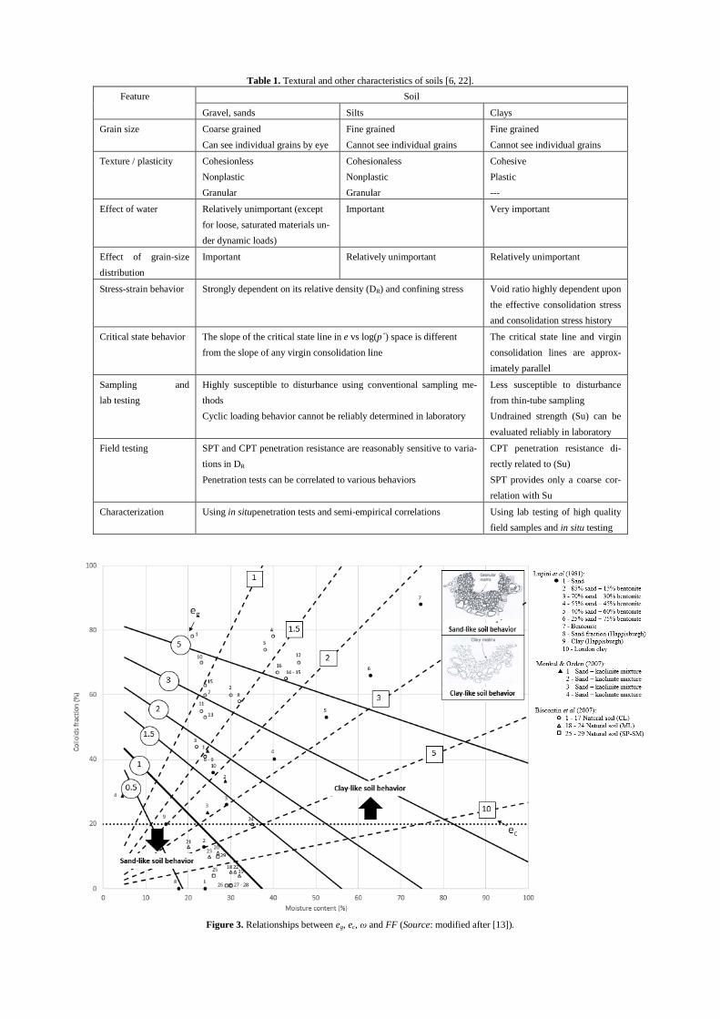
Table 1. Textural and other characteristics of soils [6, 22]. Feature Soil
Gravel, sands Silts Clays
Grain size Coarse grained Can see individual grains by eye
Fine grained Cannot see individual grains
Fine grained Cannot see individual grains
Texture / plasticity Cohesionless Nonplastic Granular
Cohesionaless Nonplastic Granular
Cohesive Plastic ---
Effect of water Relatively unimportant (except for loose, saturated materials un-der dynamic loads)
Important Very important
Effect of grain-size distribution
Important Relatively unimportant Relatively unimportant
Stress-strain behavior Strongly dependent on its relative density (DR) and confining stress Void ratio highly dependent upon the effective consolidation stress and consolidation stress history
Critical state behavior The slope of the critical state line in e vs log(p´) space is different from the slope of any virgin consolidation line
The critical state line and virgin consolidation lines are approx-imately parallel
Sampling and lab testing
Highly susceptible to disturbance using conventional sampling me-thods Cyclic loading behavior cannot be reliably determined in laboratory
Less susceptible to disturbance from thin-tube sampling Undrained strength (Su) can be evaluated reliably in laboratory
Field testing SPT and CPT penetration resistance are reasonably sensitive to varia-tions in DR Penetration tests can be correlated to various behaviors
CPT penetration resistance di-rectly related to (Su) SPT provides only a coarse cor-relation with Su
Characterization Using in situpenetration tests and semi-empirical correlations Using lab testing of high quality field samples and in situ testing
Figure 3. Relationships between eg, ec, ω and FF (Source: modified after [13]).
4.1. Discriminant analysis Discriminant analysis is a multivariate statistical
technique from which variables that differentiate groups can be identified, as well as establishing how many of these variables are necessary to achieve the best possible classification. The ultimate goal of discriminant analysis is to obtain the linear combination of independent variables that best differentiates groups. Once the discriminant functions have been obtained, they can be used to classify new cases [24]. Discriminant function have the form: 𝐷𝐷 = 𝑏𝑏1𝑋𝑋1 + 𝑏𝑏2𝑋𝑋2 + ⋯+ 𝑏𝑏𝑛𝑛𝑋𝑋𝑛𝑛 (4) Where b1, b2,..., bnare the weights of the independent
variables that make the subjects of one of the groups have maximum scores in D, and the subjects of another minimum score.
In order to carry out the discriminant analysis, it is necessary to consider several assumptions, the two most important of which are the following: (1) the matrices of covariances within each group should be approximately equal; and (2) the continuous variables should follow a normal multivariate distribution. However, the above assumptions are not usually verified in practice, because the variables usually do not have normal distributions, and most models assume equality of convariances, which is not always the case [25].
The mathematical model of the discriminant method can be revised in several references [26, 27] and papers [24, 28].
4.2. Kriging The technique known as kriging [29] consists of
obtaining linear estimators of minimum variance (Best Linear Unbiased Estimation or BLUE). Usually, kriging is applied considering that the field is wide-sense stationary (constant expected value and autocovariance depending only on the distance between the two points considered). Ordinary kriging can be expressed as follow: 𝑉𝑉∗(X) = ∑ 𝜆𝜆𝑖𝑖𝑉𝑉𝑖𝑖0
𝑖𝑖=1 + [1 − ∑ 𝜆𝜆𝑖𝑖𝑛𝑛𝑖𝑖=1 ]𝜇𝜇𝑉𝑉 (5)
Where V*(X) is the expected value as function of X; λi is a weighting factor; Vi is a value of a function at the point i; and μVis the field´s constant expected value.
It is possible to find an unbiased linear estimator with minimal variance that requires no knowledge of the mean μV, by imposing the condition: ∑ 𝜆𝜆𝑖𝑖0𝑖𝑖=1 = 1 (6)
In variogram terms, the ordinary kriging system can be written as follows: ∑ 𝜆𝜆𝑖𝑖𝛾𝛾𝑖𝑖𝑖𝑖0𝑖𝑖=1 − 𝜇𝜇 = 𝛾𝛾𝑖𝑖0´ (7)
The condition expressed by Eq.(6) must be met. The common practice in geostatistics is to calculate
the values of the theoretical semivariogram and then, for reasons of calculation efficiency, subtract some constant value from them. The end result is that geostatists eventually solve the equations of ordinary kriging in terms of covariances, even when initial calculations are made from semivariograms.
Reference [30] includes detailed information about variogramas and ordinary kriging.
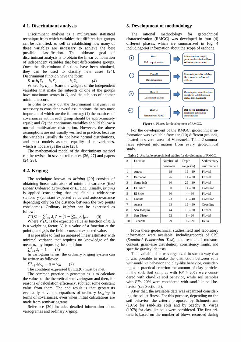
5. Development of methodology The rational methodology for geotechnical
characterization (RMGC) was developed in four (4) different phases, which are summarized in Fig. 4 includingbrief information about the scope of eachone.
Figure 4. Phases for development of RMGC.
For the development of the RMGC, geotechnical in-formation was available from ten (10) different grounds, located in several areas of Venezuela. Table 2 summa-rizes relevant information from every geotechnical study.
Table 2. Available geotechnical studies for development of RMGC. # Location Number of
boreholes Depth range (m)
Sedimentary environment
1 Anaco 99 15 – 30 Fluvial
2 Barbacoa 26 14 – 30 Fluvial
3 Santa Inés 30 25 – 30 Fluvial
4 El Palito 80 14 – 30 Coastline
5 El Sitio 30 4 – 30 Fluvial
6 Guanta 23 30 – 40 Coastline
7 Araya 63 15 – 90 Coastline
8 San Joaquín 44 15 – 30 Fluvial
9 San Diego 52 8 – 20 Fluvial
10 Tucupita 29 15 - 20 Delta From these geotechnical studies,field and laboratory
information were available, includingrecords of SPT (Standard Penetration Test), and results of moisture content, grain-size distribution, consistency limits, and specific gravity lab tests.
The available data was organized in such a way that it was possible to make the distinction between soils withsand-like behavior and clay-like behavior, consider-ing as a practical criterion the amount of clay particles in the soil. Soil samples with FF ≥ 20% were consi-dered with clay-like soil behavior, while soil samples with FF< 20% were considered with sand-like soil be-havior (see Section 3).
After that, the available data was organized consider-ing the soil stiffness. For this purpose, depending on the soil behavior, the criteria proposed by Schmertmann (1975) for sand-like soils and by Szechy & Varga (1978) for clay-like soils were considered. The first cri-teria is based on the number of blows recorded during
the performance of the SPT and the relative density of the soils; and the second one is based on the value of the Liquidity Index (LI). These criteria are summarized in Tables 3 and 4. The mentioned tables include assigned values for soil stiffness: 1 to 5 for sand-like soils, and 1 to 3 for clay-like soils.
Table 3. Criteria to estimate soil stiffness for sand-like soils. NSPT (blows/ft)
Relative den-sity (DR)
Stiffness (ST)
Assigned value of ST
0 – 4 Very loose Low
1
4 – 10 Loose 2
10 – 30 Medium Medium 3
30 – 50 Dense High
4
> 50 Very dense 5 NSPT = blows/ft recorded during SPT.
Table 4. Criteria to estimate soil stiffness for clay-like soils. LI (%)
Consistency Stiffness (ST)
Assigned value of ST
> 0.50 Very soft Low 1
0.25 – 0.50 Soft
0.00 – 0.25 Stiff Medium 2
-0.50 – 0.00 Hard High 3
< -0.50 Very hard LI = Liquidty index = (ω – PL) / (LL – PL) ω = moisture content; PL = plastic limit; LL = liquid limit. A total of 1,169 samples were available for this
study. Once the available data was discriminated, the number of samples of sand-like soils was 243, while that of clay-like soils was 926.The discriminant analyses were carried out for the groups conformed for sand-like soils and for clay-like soils, in order to obtain discrimi-nant functions for both soil types separately. The soft-ware SPSS 19.0.0 (IBM, 2010) was used to perform the analyses. Soil stiffness was selected as dependent varia-ble, considering values between 1 and 5 for sand-like soils, and between 1 and 3 for clay-like soils, as showed in Tables 3 and 4. Soil properties usually determined in routine geotechnical studies were considered as inde-pendent variables, such as NSPT, Pass#200, FF, LL, PL, PI, ω, LI and Gs.For each variable used in the analyses, and for each soil stiffness value, statistical techniques were applied to determine the following statistical pa-rameters: average, 95% confidence interval, standard deviation, standard error, and minimum and maximum values.In order to check whether the variables used for the analyses have a normal distribution, the Kolmogo-rov-Smirnov test was applied. According to this test, if the statistic Z is below 0.05, this means that the ana-lyzed variable does not have a normal distribution.A correlation matrix was elaborated, the KMO index was determined, and the Bartlett sphericity test was carried out, in order to analyze the degree of dependence be-tween the variables. According to these criteria, when the determinant of the correlation matrix is close to 0, the KMO index is greater than 0.7, and Bartlett's test is significant (Sig less than 0.05), the variables would be related to each other. In order to verify whether there are significant differences between the populations of the dependent variable for the values of the different in-
dependent variables, the ANOVA analyses were carried out. This analysis is based on the F statistic, which is distributed according to the F probability model of Fisher-Snedecor. The F statistic is interpreted in such a way that if Sig< 0.05 the hypothesis of equality of aver-ages is rejected and it is concluded that not all the com-pared population averages are equal. Finally, discrimi-nant analyses were carried out to differentiate the stiffness of different soil samples, both for sand-like and clay-like soils. To obtain information on the signific-ance of each quantitative variable in the discriminant function, the step-by-step inclusion strategy was consi-dered. Once the discriminant analysis had been per-formed for each soil type, the discriminant soil stiffness functions were determined. Table 5 shows relevant in-formation for the performed analyses.
According to the information shown in Table 5, the value of Sig in the Kolmogorov-Smirnov test is less than 0.05 in 75% of the cases for sand-like soils, and 90% of the cases for clay-like soils. Therefore, it can be considered that, in general, the variables used in the analyses do not have a normal distribution. This is in line with previous studies on the statistical distribution of geotechnical parameters [31].
Regarding the dependency between variables, the values of the determinant of the correlation matrix (D), KMO index and Bartlett's sphericity test show that there is some correlation between the variables. However, even when the value of D is close to 0, the coefficients of the correlation matrix generally do not come close to 1, so theexisting correlations would not be of good quality.The ANOVA analyses for sand-like behavior samples, showed that the statistic Fhas a Sig<0.05 for all variables, except for the variable Gs. Therefore, it is concluded that the averages of the distributions of the quantitative variables in each group are not equal, except in the case of variable Gs. For clay-like behavior soil samples, the statistic Fhas a Sig<0.05 for all variables, except for the variables Pass#200 and LL. So, it is concluded that the averages of the distributions of the quantitative variables in each group are not equal, except in the case of variables Pass#200 and LL. It is important to mention that normality of the variables is a requirement to perform the ANOVA test. However, even though distributions of quantitative variables are not normal in most cases, the ANOVA analysis is valid due to the significant number of samples considered, as well as due to means of each group present significant differences [32].Table 6 includes the discriminant func-tions obtained for each case.
In order to analyze the validity of the obtained dis-criminant functions in relation to their ability to analyze new cases, the classification matrix was constructed for both sand-like and clay-like soils. These matrices made it possible to determine the number of cases well eva-luated by the discriminant functions. Tables 7 and 8 show the classification matrices for sand-like and clay-like soils,respectively.
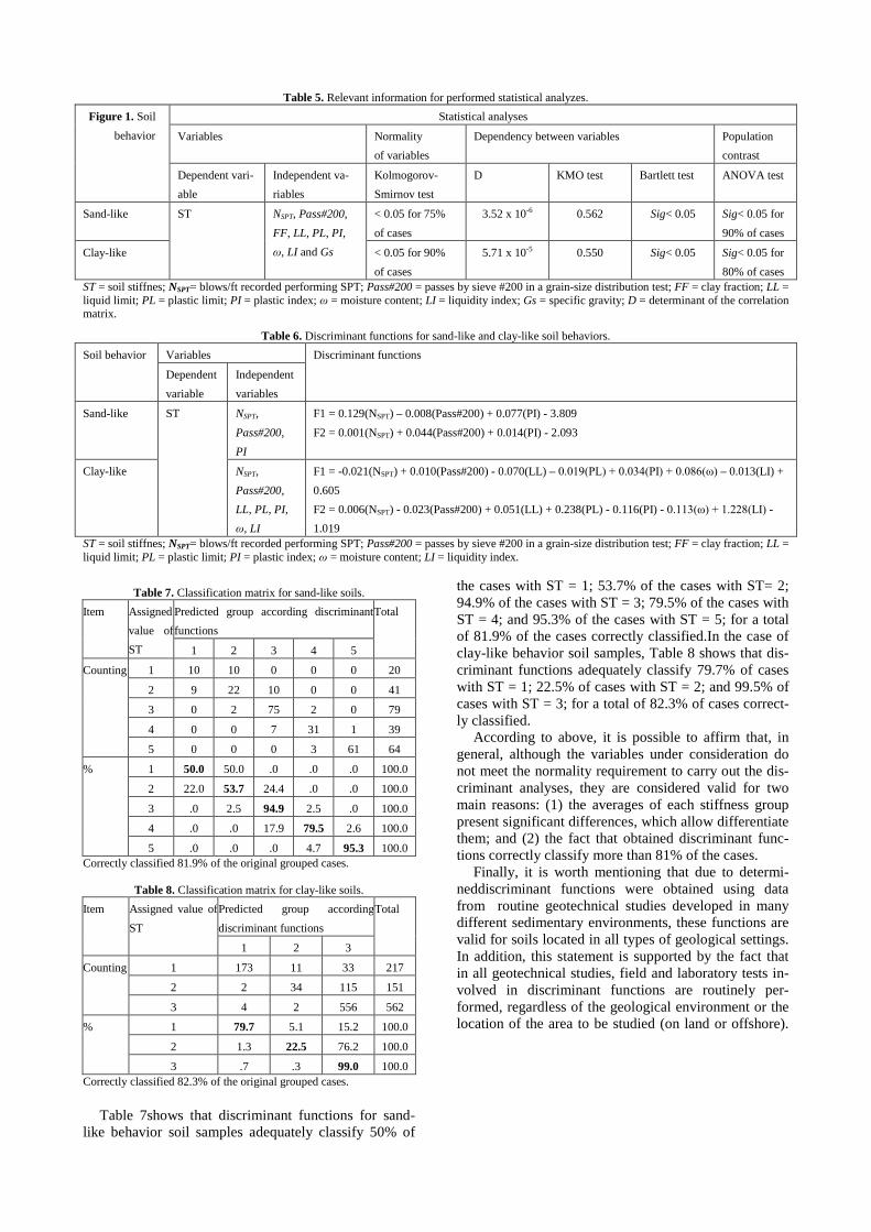
Table 5. Relevant information for performed statistical analyzes. Figure 1. Soil
behavior Statistical analyses
Variables Normality of variables
Dependency between variables Population contrast
Dependent vari-able
Independent va-riables
Kolmogorov-Smirnov test
D KMO test Bartlett test ANOVA test
Sand-like ST NSPT, Pass#200, FF, LL, PL, PI, ω, LI and Gs
< 0.05 for 75% of cases
3.52 x 10⁻⁶ 0.562 Sig< 0.05 Sig< 0.05 for 90% of cases
Clay-like < 0.05 for 90% of cases
5.71 x 10⁻⁵ 0.550 Sig< 0.05 Sig< 0.05 for 80% of cases
ST = soil stiffnes; NSPT= blows/ft recorded performing SPT; Pass#200 = passes by sieve #200 in a grain-size distribution test; FF = clay fraction; LL = liquid limit; PL = plastic limit; PI = plastic index; ω = moisture content; LI = liquidity index; Gs = specific gravity; D = determinant of the correlation matrix.
Table 6. Discriminant functions for sand-like and clay-like soil behaviors. Soil behavior Variables Discriminant functions
Dependent variable
Independent variables
Sand-like ST NSPT, Pass#200, PI
F1 = 0.129(NSPT) – 0.008(Pass#200) + 0.077(PI) - 3.809 F2 = 0.001(NSPT) + 0.044(Pass#200) + 0.014(PI) - 2.093
Clay-like NSPT, Pass#200, LL, PL, PI, ω, LI
F1 = -0.021(NSPT) + 0.010(Pass#200) - 0.070(LL) – 0.019(PL) + 0.034(PI) + 0.086(ω) – 0.013(LI) + 0.605 F2 = 0.006(NSPT) - 0.023(Pass#200) + 0.051(LL) + 0.238(PL) - 0.116(PI) - 0.113(ω) + 1.228(LI) - 1.019
ST = soil stiffnes; NSPT= blows/ft recorded performing SPT; Pass#200 = passes by sieve #200 in a grain-size distribution test; FF = clay fraction; LL = liquid limit; PL = plastic limit; PI = plastic index; ω = moisture content; LI = liquidity index.
Table 7. Classification matrix for sand-like soils. Item Assigned
value of ST
Predicted group according discriminant functions
Total
1 2 3 4 5
Counting 1 10 10 0 0 0 20
2 9 22 10 0 0 41
3 0 2 75 2 0 79
4 0 0 7 31 1 39
5 0 0 0 3 61 64
% 1 50.0 50.0 .0 .0 .0 100.0
2 22.0 53.7 24.4 .0 .0 100.0
3 .0 2.5 94.9 2.5 .0 100.0
4 .0 .0 17.9 79.5 2.6 100.0
5 .0 .0 .0 4.7 95.3 100.0 Correctly classified 81.9% of the original grouped cases.
Table 8. Classification matrix for clay-like soils.
Item Assigned value of ST
Predicted group according discriminant functions
Total
1 2 3
Counting 1 173 11 33 217
2 2 34 115 151
3 4 2 556 562
% 1 79.7 5.1 15.2 100.0
2 1.3 22.5 76.2 100.0
3 .7 .3 99.0 100.0 Correctly classified 82.3% of the original grouped cases.
Table 7shows that discriminant functions for sand-like behavior soil samples adequately classify 50% of
the cases with ST = 1; 53.7% of the cases with ST= 2; 94.9% of the cases with ST = 3; 79.5% of the cases with ST = 4; and 95.3% of the cases with ST = 5; for a total of 81.9% of the cases correctly classified.In the case of clay-like behavior soil samples, Table 8 shows that dis-criminant functions adequately classify 79.7% of cases with ST = 1; 22.5% of cases with ST = 2; and 99.5% of cases with ST = 3; for a total of 82.3% of cases correct-ly classified.
According to above, it is possible to affirm that, in general, although the variables under consideration do not meet the normality requirement to carry out the dis-criminant analyses, they are considered valid for two main reasons: (1) the averages of each stiffness group present significant differences, which allow differentiate them; and (2) the fact that obtained discriminant func-tions correctly classify more than 81% of the cases.
Finally, it is worth mentioning that due to determi-neddiscriminant functions were obtained using data from routine geotechnical studies developed in many different sedimentary environments, these functions are valid for soils located in all types of geological settings. In addition, this statement is supported by the fact that in all geotechnical studies, field and laboratory tests in-volved in discriminant functions are routinely per-formed, regardless of the geological environment or the location of the area to be studied (on land or offshore).
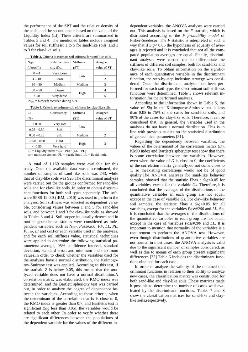
6. Formulation of RMGC The rational methodology for geotechnical
characterization (RMGC)is based on the discriminant functions obtained for sand-like and clay-like soils. The results of the performed discriminant analyses will constitute characterization factors: C1 and C2 for sand-like soils; and F1 and F2 for clay-like soils. Graphs of relationships between those factors were prepared, in order to classified new cases depending on the values of such factors. Those graphs are showed in Fig. 5 and Fig. 6, which include the functions to determine characterization factors.
Figure 5. Characterization factors graph for sand-like soils.
Figure 6. Characterization factors graph for clay-like soils.
Thus, given a soil sample, the values of C1 and C2 or F1 and F2 (depending on their expected behaviour)are determined. Then, these values are plotted in the graphs shown in Fig. 5 or Fig. 6 (as appropriate) and, depending on the location of the resulted point in the graph, a stiffness value is assigned.
The following is a step-by-step RMGC, based on information available from routine geotechnical studies:
1. Identify the different strata detected in a borehole, and assume that the properties determined in the samples obtained from a given stratum are representative of the entire
stratum (this is a common practice in Geotechnics, since not all samples are tested, but only some representative ones).
2. For each defined strata, consider the following:
• If the soil has Pass#200 ≥ 50% (silt or clay), and a grain-size analysis is not available, assume Pass#200 = 51%.
• If the soil has Pass#200 < 50% (sand or gravel), the FF value is significant when FF ≥ 20%. Thus, if a hydrometer test is not available, it is needed to verified that Pass#200 is less than 20%; if this occurs, the effect of the fine fraction is not appreciable in the soil behaviour.
• If the soil sample is non-plastic (NP), LL = 1 and PL = 0 must be assumed. These values correspond to soils located in the lower left sector of the Casagrande Charter for fine soils, with little or very low plasticity.
• For soils in which it was necessary to advance drilling by rotation (very hard or very dense soils), assume a value of NSPT = 100 blows/ft.
3. From performed laboratory tests, determine whether the stratum presents a sand-like or clay-like behaviour.
4. Determine soil stiffness for all available soil samples using the characterization factores C1 and C2 for sand-like soils, and F1 and F2 for clay-like soils.
5. Group the data relating to soil stiffness and soil behaviour as considered appropriate (it can be, for example, meter by meter; or for significant strata detected in the ground, depending on the criteria of the Geotechnical Engineer).
6. Generate the Geotechnical Zoning Map, using geostatistics (for instance, kriging). For this, any available software in the market can be used. This map will allow to identify sectors of the ground with different stiffness.
7. Generate a Soil Behavior Map, also using geostatistics. This map can easily be superimposed on the previous one and thus identify sectors of the ground that present sand-like or clay-like behavior, with its corresponding stiffness.
It is worth mentioning that the application of the proposed methodology requires a carefull reviewing and systematic organization of field and lab data. In addition, it should be noted that thedeveloped methodology constitute a tool that supplement, but does not substitute, traditional interpolation criteria based on geological evidences, and in particular geomorphology and sedimentology.
Using this practical methodology, zoning and soil-behavior maps will be generated, which will allow to make an evaluation of the probability of reaching or exceeding locally some extreme conditions that could be critical for the project under study.
Characterization factor C1
Cha
ract
eriz
atio
n fa
ctor
C2 ST = 1
ST = 2
ST = 3
ST = 4
ST = 5
C1 = 0.129(NSPT) – 0.008(Pass#200) + 0.077(PI) - 3.809 C2 = 0.001(NSPT) + 0.044(Pass#200) + 0.014(PI) - 2.093
Characterization factor F1
Cha
ract
eriz
atio
n fa
ctor
F2
ST = 1
ST = 2
ST = 3
F1 = -0.021(NSPT) + 0.010(Pass#200) - 0.070(LL) – 0.019(PL) + 0.034(PI) + 0.086(ω) – 0.013(LI) + 0.605
F2 = 0.006(NSPT) - 0.023(Pass#200) + 0.051(LL) + 0.238(PL) - 0.116(PI) - 0.113(ω) + 1.228(LI) - 1.019
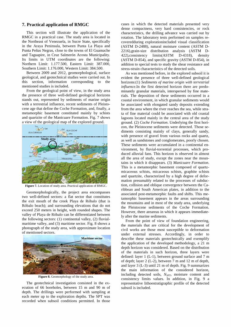
7. Practical application of RMGC This section will illustrate the application of the
RMGC in a practical case. The study area is located in the Northeast of Venezuela, in Sucre State, specifically in the Araya Peninsula, between Punta La Playa and Punta Peñas Negras, close to the towns of El Guamache and Taguapire, in Cruz Salmerón Acosta Municipality. Its limits in UTM coordinates are the following: Northern Limit: 1.177.500, Eastern Limit: 387.000, Southern Limit: 1.176.000, Western Limit: 384.500.
Between 2009 and 2012, geomorphological, surface geological, and geotechnical studies were carried out. In this section, information corresponding to the mentioned studies is included.
From the geological point of view, in the study area the presence of three well-defined geological horizons stands out, represented by sediments of marine origin with a terrestrial influence, recent sediments of Pleisto-cene age that define the Coche Formation, and, finally, a metamorphic basement constituted mainly by schists and quartzite of the Manicuare Formation. Fig. 7 shows a view of the geological map of the explored ground.
Figure 7. Location of study area. Practical application of RMGC.
Geomorphologically, the project area encompasses two well-defined sectors: a flat sector that constitutes the exit mouth of the creek Playa de Róbalo (that is Róbalo beach); and surrounding elevations that do not exceed 250 meters in height, with rounded shapes. The valley of Playa de Róbalo can be differentiated between the following sectors: (1) continental valley, (2) fluvial-maritime valley, and (3) maritime sector. Fig. 8 shows a photograph of the study area, with approximate location of mentioned sectors.
Figure 8. Geomorphology of the study area.
The geotechnical investigation consisted in the ex-ecution of 66 boreholes, between 15 m and 90 m of depth. The drillings were performed with sampling at each meter up to the exploration depths. The SPT was recorded when subsoil conditions permitted. In those
cases in which the detected materials presented very dense compactness, very hard consistencies, or rock characteristics, the drilling advance was carried out by rotation. The laboratory tests performed on samples re-coveredduring explorationincluded visual classification (ASTM D-2488), natural moisture content (ASTM D-2216),grain-size distribution analysis (ASTM D-422),consistency limits(ASTM D-4318), density (ASTM D-854), and specific gravity (ASTM D-854), in addition to special tests to study the shear resistance and stress-strain characteristics of the detected soils.
As was mentioned before, in the explored subsoil it is evident the presence of three well-defined geological horizons:(1) Sediments of marine origin with terrestrial influence.In the first detected horizon there are predo-minantly granular materials, interspersed by fine mate-rials. The deposition of these sediments occurred in a coastal environment, in which granular sediments would be associated with elongated sandy deposits extending from the area where the river reaches the sea, while stra-ta of fine material could be associated with old coastal lagoons located mainly in the central area of the study ground. (2) Coche Formation. Underlying the first hori-zon, the Pleistocene sediments were detected. Those se-diments consisting mainly of clays, generally sandy, with presence of gravel from various rocks and quartz, as well as sandstones and conglomerates, poorly chosen. These sediments were accumulated in a continental en-vironment, by fluvial-torrential processes, which pro-duced alluvial fans. This horizon is observed in almost all the area of study, except the zones near the moun-tains in which it disappears. (3) Manicuare Formation. This is a metamorphic basement composed of quartz-micaceous schists, micaceous schists, graphite schists and quartzite, characterized by a high degree of defor-mation presumably related to the processes of subduc-tion, collision and oblique convergence between the Ca-ribbean and South American plates, in addition to the associated post-metamorphic faults and shifts. This me-tamorphic basement appears in the areas surrounding the mountains and in most of the study area, underlying the Pleistocene sediments of the Coche Formation. However, there areareas in which it appears immediate-ly after the marine sediments.
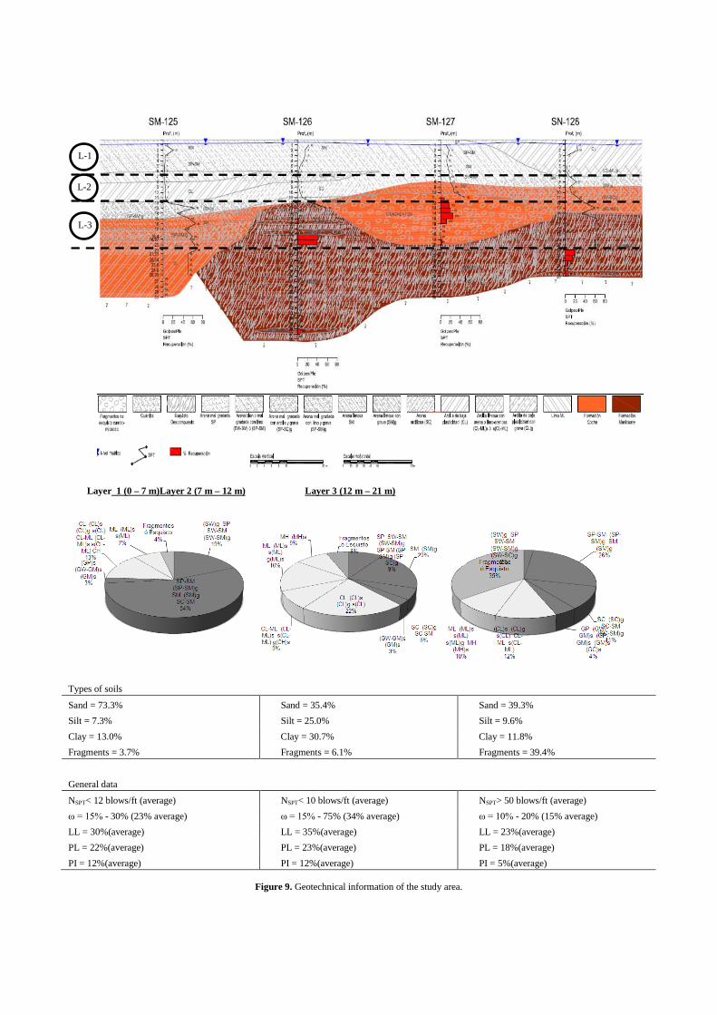
From the point of view of foundation engineering, the materials that are critical for the development of civil works are those most susceptible to deformation under external stresses. Accordingly, in order to describe these materials geotechnically and exemplify the application of the developed methodology, a 21 m depth horizon was considered. Based on the distribution of the materials in such horizon, three layers were defined: layer 1 (L-1), between ground surface and 7 m of depth; layer 2 (L-2), between 7 m and 12 m of depth, and layer 3 (L-3) until 21 m of depth. Fig. 9 summarizes the main information of the considered horizon, including detected soils, NSPT, moisture content and consistency limits values. In addition, in Fig. 9 a representative lithoestratigraphic profile of the detected subsoil is included.
Maritime sector
Fluvial-maritime valley
Continental valley
Study area
Layer 1 (0 – 7 m)Layer 2 (7 m – 12 m)
Layer 3 (12 m – 21 m)
Types of soils
Sand = 73.3% Sand = 35.4% Sand = 39.3% Silt = 7.3% Silt = 25.0% Silt = 9.6% Clay = 13.0% Clay = 30.7% Clay = 11.8% Fragments = 3.7% Fragments = 6.1% Fragments = 39.4%
General data
NSPT< 12 blows/ft (average) NSPT< 10 blows/ft (average) NSPT> 50 blows/ft (average) ω = 15% - 30% (23% average) ω = 15% - 75% (34% average) ω = 10% - 20% (15% average) LL = 30%(average) LL = 35%(average) LL = 23%(average) PL = 22%(average) PL = 23%(average) PL = 18%(average) PI = 12%(average) PI = 12%(average) PI = 5%(average)
Figure 9. Geotechnical information of the study area.
L-1
L-2
L-3
It should be noted that moisture content values are relatively close to PL in L-1 and L-3, while in L-2 these values are close to LL. This fact evidences that L-2 presents high compressibility fines (in approximately 10% of the stratum), represented mainly by high com-pressibility silt (MH), high compressibility silt with sand (MH)s, and high compressibility clay with sand g(CH)s; with moisture content values higher than LL, which indicates that they are in a consistency similar to a sludge. This is also reflected in the NSPT values record-ed during fieldworks.
At the time of executing the fieldwork, the water ta-ble was detected at variable depths between 0.30 m and 1.50 m, with an average value of 0.75 m. Such values were obtained from daily measurements taken early in the morning.
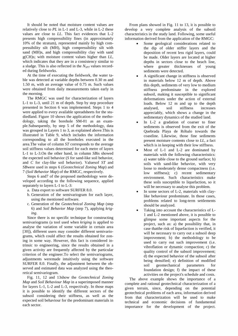
The RMGC was used for characterization of layers L-1 to L-3, until 21 m of depth. Step by step procedure presented in Section 6 was implemented. Steps 1 to 4 were applied to every available spreadsheets for the stu-diedland. Figure 10 shows the application of the metho-dology, taking the borehole SM-01 as an exam-ple.Subsequently, by step 5 of the methodology, data was grouped in Layers 1 to 3, as explained above.This is illustrated in Table 9, which includes the information corresponding to all the boreholes executed in the area.The value of column ST corresponds to the average soil stiffness values determined for each metre of layers L-1 to L-3.On the other hand, in column SBis showed the expected soil behavior (S for sand-like soil behavior, and C for clay-like soil behavior). Valuesof ST and SBwere used in steps 6 (Geotechnical Zoning Map) and 7 (Soil Behavior Map) of the RMGC, respectively.
Steps 6 and7 of the proposed methodology were de-veloped according to the following sequence, applied separately to layers L-1 to L-3:
a. Data export to software SURFER 8.0. b. Generation of the semivariogram for each layer,
using the mentioned software. c. Generation of the Geotechnical Zoning Map (step
6) and Soil Behavior Map (step 7), applying krig-ing.
Since there is no specific technique for constructing semivariograms (a tool used when kriging is applied to analyse the variation of some variable in certain area [30]), different users may consider different semivario-grams, which could affect the results obtained for zon-ing in some way. However, this fact is considered in-trinsic to engineering, since the results obtained in a given activity are frequently affected by the particular criterion of the engineer.To select the semivariograms, adjustments weremade intuitively using the software SURFER 8.0. Finally, the adjustment between the ob-served and estimated data was analyzed using the theo-retical semivariogram.
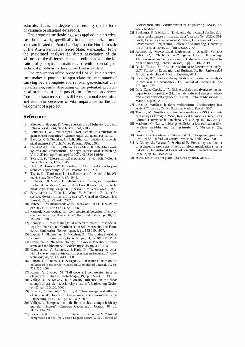
Fig. 11, 12 and 13show the Geotechnical Zoning Map and Soil Behaviour Map in a superimposed manner for layers L-1, L-2 and L-3, respectivaly. In those maps it is possible to identify the different sectors of the subsoil considering their stiffness, as well as the expected soil behaviour for the predominant materials in each sector.
From plans showed in Fig. 11 to 13, it is possible to develop a very complete analysis of the subsoil characteristics in the study land. Following, some useful information derived from the application of the RMGC:
• Some geological considerations related to the dip of older stiffer layers and the deposition of recent less rigid layers, could be made. Older layers are located at higher depths in sectors close to the beach line, where greater thicknesses of young sediments were detected.
• A significant change in stiffness is observed in materials below 12 m of depth. Above this depth, sediments of very low to medium stiffness predominate in the explored subsoil, making it susceptible to significant deformations under the action of external loads. Below 12 m and up to the depth analysed, soil stiffness increases appreciably, which shows a change in the sedimentary dynamics of the studied land.
• In L-2 a gradation of coarser to finer sediments is observed from the exit of the Quebrada Playa de Róbalo towards the coastline. Likewise, those fine sediments present moisture contents close to LL, a fact which is in keeping with their low stiffness.
• Most of L-1 and L-2 are dominated by materials with the following characteristics: a) water table close to the ground surface; b) soils with sand-like behavior, with very loose to moderately dense compactness (i.e. low stiffness); c) recent sedimentary environment. Such characteristics make these soils susceptible to liquefaction, so it will be necessary to analyse this problem.
• In some sectors of L-2, materials with clay-like behaviour predominate. In those cases, problems related to long-term settlements should be analyzed.
• Taking into account the characteristics of L-1 and L-2 mentioned above, it is possible to glimpse some important aspects for the project, such as: a) the possibility that, in case thatthe risk of liquefaction is verified, it will be necessary to carry out a subsoil deep improvement; b) the methodology to be used to carry out such improvement (i.e. vibroflation or dynamic compaction; c) the quality control of the subsoil improvement; d) the expected behavior of the subsoil after being densified; e) definition of modified soil geomechanical parameters for foundation design; f) the impact of these activities on the project's schedule and costs.
The above example shows the importance of a complete and rational geotechnical characterization of a given terrain, since, depending on the potential geotechnical problems of each area, information derived from that characterization will be used to make technical and economic decisions of fundamental importance for the development of the project.
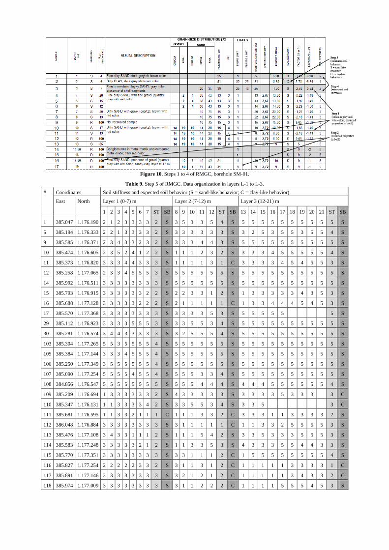
Figure 10. Steps 1 to 4 of RMGC, borehole SM-01.
Table 9. Step 5 of RMGC. Data organization in layers L-1 to L-3. # Coordinates Soil stiffness and expected soil behavior (S = sand-like behavior; C = clay-like behavior)
East North Layer 1 (0-7) m Layer 2 (7-12) m Layer 3 (12-21) m
1 2 3 4 5 6 7 ST SB 8 9 10 11 12 ST SB 13 14 15 16 17 18 19 20 21 ST SB
1 385.047 1.176.190 2 1 2 3 3 3 3 2 S 3 5 3 3 5 4 S 5 5 5 5 5 5 5 5 5 5 S
5 385.194 1.176.333 2 2 1 3 3 3 3 2 S 3 3 3 3 3 3 S 3 2 5 3 5 5 3 5 5 4 S
9 385.585 1.176.371 2 3 4 3 3 2 3 2 S 3 3 3 4 4 3 S 5 5 5 5 5 5 5 5 5 5 S
10 385.474 1.176.605 2 3 5 2 4 1 2 2 S 1 1 1 2 3 2 S 3 3 3 4 5 5 5 5 5 4 S
11 385.373 1.176.820 3 3 3 4 4 3 3 3 S 1 1 1 1 3 1 C 3 3 3 3 4 5 4 5 5 3 S
12 385.258 1.177.065 2 3 3 4 5 5 5 3 S 5 5 5 5 5 5 S 5 5 5 5 5 5 5 5 5 5 S
14 385.992 1.176.511 3 3 3 3 3 3 3 3 S 5 5 5 5 5 5 S 5 5 5 5 5 5 5 5 5 5 S
15 385.793 1.176.915 3 3 3 3 3 3 2 2 S 2 2 3 3 1 2 S 1 3 3 3 3 3 4 3 5 3 S
16 385.688 1.177.128 3 3 3 3 3 2 2 2 S 2 1 1 1 1 1 C 1 3 3 4 4 4 5 4 5 3 S
17 385.570 1.177.368 3 3 3 3 3 3 3 3 S 3 3 3 3 5 3 S 5 5 5 5 5
5 S
29 385.112 1.176.923 3 3 3 3 5 5 5 3 S 3 3 5 5 3 4 S 5 5 5 5 5 5 5 5 5 5 S
30 385.281 1.176.574 3 4 4 3 3 3 3 3 S 3 2 5 5 5 4 S 5 5 5 5 5 5 5 5 5 5 S
103 385.304 1.177.265 5 5 3 5 5 5 5 4 S 5 5 5 5 5 5 S 5 5 5 5 5 5 5 5 5 5 S
105 385.384 1.177.144 3 3 3 4 5 5 5 4 S 5 5 5 5 5 5 S 5 5 5 5 5 5 5 5 5 5 S
106 385.250 1.177.349 3 5 5 5 5 5 5 4 S 5 5 5 5 5 5 S 5 5 5 5 5 5 5 5 5 5 S
107 385.090 1.177.254 5 5 5 5 4 5 5 4 S 5 5 5 3 3 4 S 5 5 5 5 5 5 5 5 5 5 S
108 384.856 1.176.547 5 5 5 5 5 5 5 5 S 5 5 5 4 4 4 S 4 4 4 5 5 5 5 5 5 4 S
109 385.209 1.176.694 1 3 3 3 3 3 3 2 S 4 3 3 3 3 3 S 3 3 3 3 5 3 3 3
3 C
110 385.347 1.176.131 1 1 3 3 3 3 4 2 S 3 3 5 5 3 4 S 3 3 5
3 C
111 385.681 1.176.595 1 1 3 3 2 1 1 1 C 1 1 1 3 3 2 C 3 3 3 1 1 3 3 3 3 2 S
112 386.048 1.176.884 3 3 3 3 3 3 3 3 S 3 1 1 1 1 1 C 1 1 3 3 2 5 5 5 5 3 S
113 385.476 1.177.108 3 4 3 3 1 1 1 2 S 1 1 1 5 4 2 S 3 3 5 3 3 3 5 5 5 3 S
114 385.583 1.177.248 3 3 3 3 3 2 1 2 S 1 1 3 3 5 3 S 4 3 3 3 5 5 4 4 3 3 S
115 385.770 1.177.351 3 3 3 3 3 3 3 3 S 3 3 1 1 1 2 C 1 5 5 5 5 5 5 5 5 4 S
116 385.827 1.177.254 2 2 2 2 2 3 3 2 S 3 1 1 3 1 2 C 1 1 1 1 1 3 3 3 3 1 C
117 385.891 1.177.146 3 3 3 3 3 3 3 3 S 3 2 1 2 1 2 C 1 1 1 1 1 3 4 3 3 2 C
118 385.974 1.177.009 3 3 3 3 3 3 3 3 S 3 1 1 2 2 2 C 1 1 1 1 5 5 5 4 5 3 S
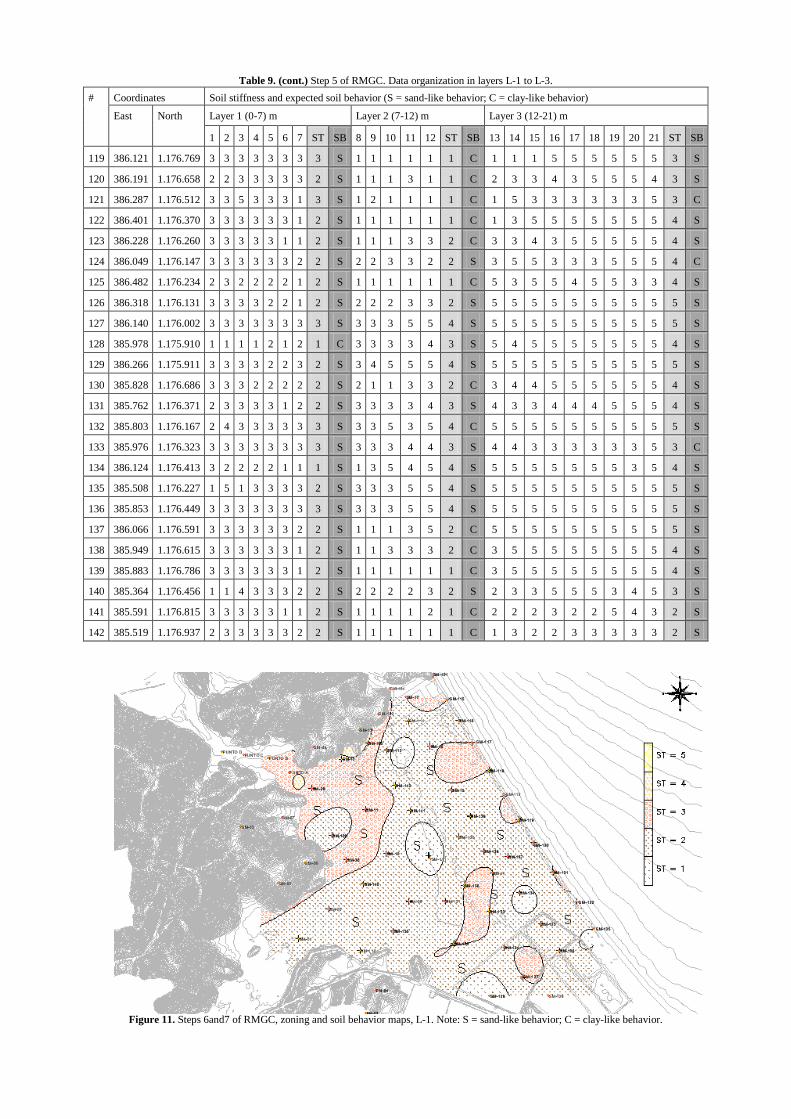
Table 9. (cont.) Step 5 of RMGC. Data organization in layers L-1 to L-3. # Coordinates Soil stiffness and expected soil behavior (S = sand-like behavior; C = clay-like behavior)
East North Layer 1 (0-7) m Layer 2 (7-12) m Layer 3 (12-21) m
1 2 3 4 5 6 7 ST SB 8 9 10 11 12 ST SB 13 14 15 16 17 18 19 20 21 ST SB
119 386.121 1.176.769 3 3 3 3 3 3 3 3 S 1 1 1 1 1 1 C 1 1 1 5 5 5 5 5 5 3 S
120 386.191 1.176.658 2 2 3 3 3 3 3 2 S 1 1 1 3 1 1 C 2 3 3 4 3 5 5 5 4 3 S
121 386.287 1.176.512 3 3 5 3 3 3 1 3 S 1 2 1 1 1 1 C 1 5 3 3 3 3 3 3 5 3 C
122 386.401 1.176.370 3 3 3 3 3 3 1 2 S 1 1 1 1 1 1 C 1 3 5 5 5 5 5 5 5 4 S
123 386.228 1.176.260 3 3 3 3 3 1 1 2 S 1 1 1 3 3 2 C 3 3 4 3 5 5 5 5 5 4 S
124 386.049 1.176.147 3 3 3 3 3 3 2 2 S 2 2 3 3 2 2 S 3 5 5 3 3 3 5 5 5 4 C
125 386.482 1.176.234 2 3 2 2 2 2 1 2 S 1 1 1 1 1 1 C 5 3 5 5 4 5 5 3 3 4 S
126 386.318 1.176.131 3 3 3 3 2 2 1 2 S 2 2 2 3 3 2 S 5 5 5 5 5 5 5 5 5 5 S
127 386.140 1.176.002 3 3 3 3 3 3 3 3 S 3 3 3 5 5 4 S 5 5 5 5 5 5 5 5 5 5 S
128 385.978 1.175.910 1 1 1 1 2 1 2 1 C 3 3 3 3 4 3 S 5 4 5 5 5 5 5 5 5 4 S
129 386.266 1.175.911 3 3 3 3 2 2 3 2 S 3 4 5 5 5 4 S 5 5 5 5 5 5 5 5 5 5 S
130 385.828 1.176.686 3 3 3 2 2 2 2 2 S 2 1 1 3 3 2 C 3 4 4 5 5 5 5 5 5 4 S
131 385.762 1.176.371 2 3 3 3 3 1 2 2 S 3 3 3 3 4 3 S 4 3 3 4 4 4 5 5 5 4 S
132 385.803 1.176.167 2 4 3 3 3 3 3 3 S 3 3 5 3 5 4 C 5 5 5 5 5 5 5 5 5 5 S
133 385.976 1.176.323 3 3 3 3 3 3 3 3 S 3 3 3 4 4 3 S 4 4 3 3 3 3 3 3 5 3 C
134 386.124 1.176.413 3 2 2 2 2 1 1 1 S 1 3 5 4 5 4 S 5 5 5 5 5 5 5 3 5 4 S
135 385.508 1.176.227 1 5 1 3 3 3 3 2 S 3 3 3 5 5 4 S 5 5 5 5 5 5 5 5 5 5 S
136 385.853 1.176.449 3 3 3 3 3 3 3 3 S 3 3 3 5 5 4 S 5 5 5 5 5 5 5 5 5 5 S
137 386.066 1.176.591 3 3 3 3 3 3 2 2 S 1 1 1 3 5 2 C 5 5 5 5 5 5 5 5 5 5 S
138 385.949 1.176.615 3 3 3 3 3 3 1 2 S 1 1 3 3 3 2 C 3 5 5 5 5 5 5 5 5 4 S
139 385.883 1.176.786 3 3 3 3 3 3 1 2 S 1 1 1 1 1 1 C 3 5 5 5 5 5 5 5 5 4 S
140 385.364 1.176.456 1 1 4 3 3 3 2 2 S 2 2 2 2 3 2 S 2 3 3 5 5 5 3 4 5 3 S
141 385.591 1.176.815 3 3 3 3 3 1 1 2 S 1 1 1 1 2 1 C 2 2 2 3 2 2 5 4 3 2 S
142 385.519 1.176.937 2 3 3 3 3 3 2 2 S 1 1 1 1 1 1 C 1 3 2 2 3 3 3 3 3 2 S
Figure 11. Steps 6and7 of RMGC, zoning and soil behavior maps, L-1. Note: S = sand-like behavior; C = clay-like behavior.
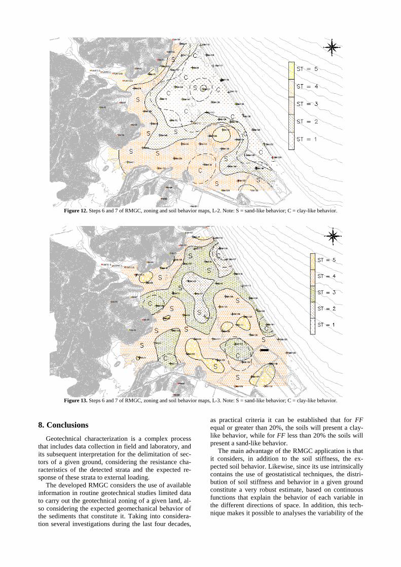
Figure 12. Steps 6 and 7 of RMGC, zoning and soil behavior maps, L-2. Note: S = sand-like behavior; C = clay-like behavior.
Figure 13. Steps 6 and 7 of RMGC, zoning and soil behavior maps, L-3. Note: S = sand-like behavior; C = clay-like behavior.
8. Conclusions Geotechnical characterization is a complex process
that includes data collection in field and laboratory, and its subsequent interpretation for the delimitation of sec-tors of a given ground, considering the resistance cha-racteristics of the detected strata and the expected re-sponse of these strata to external loading.
The developed RMGC considers the use of available information in routine geotechnical studies limited data to carry out the geotechnical zoning of a given land, al-so considering the expected geomechanical behavior of the sediments that constitute it. Taking into considera-tion several investigations during the last four decades,
as practical criteria it can be established that for FF equal or greater than 20%, the soils will present a clay-like behavior, while for FF less than 20% the soils will present a sand-like behavior.
The main advantage of the RMGC application is that it considers, in addition to the soil stiffness, the ex-pected soil behavior. Likewise, since its use intrinsically contains the use of geostatistical techniques, the distri-bution of soil stiffness and behavior in a given ground constitute a very robust estimate, based on continuous functions that explain the behavior of each variable in the different directions of space. In addition, this tech-nique makes it possible to analyses the variability of the
estimate, that is, the degree of uncertainty (in the form of variance or standard deviation).
The proposed methodology was applied in a practical case in this work, specifically in the characterization of a terrain located in Punta La Playa, on the Northern side of the Araya Peninsula, Sucre State, Venezuela. From the performed analyses,the direct association of the stiffness of the different detected sediments with the lo-cation of geological formations and with potential geo-technical problems in the studied land is evident.
The application of the proposed RMGC in a practical case makes it possible to appreciate the importance of carrying out a complete and rational geotechnical cha-racterization, since, depending on the potential geotech-nical problems of each parcel, the information derived from this characterization will be used to make technical and economic decisions of vital importance for the de-velopment of a project.
References [1] Mitchell, J. & Soga, K. "Fundamentals of soil behavior”, 3rd ed.,
John Wiley & Sons, New Jersey, USA, 2005. [2] Bourdeau P. & AmundarayJ.I. “Non-parametric simulation of
geotechnical variability”, Geotechnique, 55, pp. 95-108, 2005. [3] Baecher, G.& Christian, J. “Reliability and statistics in geotech-
nical engineering”. John Wiley & Sons, USA, 2003. [4] Shitet al(2016) Shit, P., Bhunia, G. & Maiti, R. “Modeling earth
systems and environment”. Springer International Publishing, Vol. 2, 2016. https//.doi.org/10.1007/s40808-016-0160-4.
[5] Terzaghi, K. “Theoretical soil mechanics”, 1st ed., John Wiley & Sons, New York, USA, 1943.
[6] Holtz, R., Kovacs, W. & Sheahan, T. “An introduction to geo-technical engineering”, 2nd ed., Pearson, USA, 2011.
[7] Taylor, D. “Fundamentals of soil mechanics”, 1st ed., John Wi-ley & Sons, New York, USA, 1948.
[8] Kulhawy, F.& Mayne, P. “Manual on estimating soil properties for foundation design”, prepared by Cornell University Geotech-nical Engineering Group, Hollister Hall, New York, USA, 1990.
[9] Santamarina, J., Klein, K., Wang, Y. & Prencke, E. “Specific surface: determination and relevance”, Canadian Geotechnical Journal, 39, pp. 233-241, 2002.
[10] Mitchell, J. “Fundamentals of soil behavior”, 1st ed., John Wiley & Sons, Inc., New York, USA, 1976.
[11] Monkul, M.& Ozden, G. “Compressional behavior of clayey sand and transition fines content”, Engineering Geology, 89, pp. 195-205, 2007.
[12] Kenney, T. “Residual strength of mineral mixtures”, In: Proceed-ings 9th International Conference on Soil Mechanics and Foun-dation Engineering, Tokyo, Japan, 1, pp. 155-160, 1977.
[13] Lupini, J., Skinner, A. & Vaughan, P. “The drained residual strength of cohesive soils”, Geotechnique, 31, pp. 181-212, 1981.
[14] Skempton, A. “Residual strength of clays in landslides, folded strata and the laboratory”, Geotechnique, 35, pp. 3-18, 1985.
[15] Georgiannou, V., Burland, J. & Hight, D. “The undrained beha-vior of clayey sands in triaxial compression and extension”, Geo-technique, 40, pp. 431-449, 1990.
[16] Pitman, T., Robertson, P. & Sego, D. “Influence of fines on the collapse of loose sands”, Canadian Geotechnical Journal, 31, pp. 728-739, 1994.
[17] Kumar, G. &Wood, M. “Fall cone and compression tests on clay-gravel mixtures”, Geotechnique, 49, pp. 727-739, 1999.
[18] Vallejo, L. & Mawby, R. “Porosity influence on the shear strength of granular material-clay mixtures”, Engineering Geolo-gy, 58, pp. 125-136, 2000.
[19] Salgado, R., Bandini, P. & Krim, A. “Shear strength and stiffness of silty sand”, Journal of Geotechnical and Geoenvironmental Engineering, ASCE 126, pp. 451-462, 2000.
[20] Vallejo, L. “Interpretation of the limits in shear strength in binary granular mixtures”, Canadian Geotechnical Journal, 38, pp. 1097-1104, 2001.
[21] Biscontin, G., Simonetta, C. Pestana, J. & Simonini, M. “Unified compression model for Venice Lagoon natural silts”, Journal of
Geotechnical and Geoenvironmental Engineering, ASCE, pp. 932-942, 2007.
[22] Boulanger, R.& Idriss, I. “Evaluating the potential for liquefac-tion or cyclic failure of silts and clays”, Report No. UCD/CGM-04-01, Center for Geotechnical Modeling, Department of Civil & Environmental Engineering, College of Engineering, University of California at Davis, California, USA, 2004.
[23] Auvinet, G. “Geotechnical Engineering in Spatially Variable Soft Soils”, In: The 9th Arthur Casagrande Lecture - Proceedings XVI Panamerican Conference on Soil Mechanics and Geotech-nical Engineering, Cancun, Mexico, 1, pp. 13-107, 2019.
[24] De La Fuente, S. “Análisis discriminante(Discriminant analy-sis)”, Faculty of Economics and Business Studies, Universidad Autónoma de Madrid, Madrid, Españan, 2011.
[25] Eisenbeis, R. “Pitfalls in the application of discriminant analysis in bussiness and economics”, The Journal of Finance, 32, pp. 875-900, 1977.
[26] De la Garza García, J. “Análisis estadístico multivariante: un en-foque teórico y práctico (Multivariate statistical analysis: atheo-retical and practical approach)”, 1st ed., Editorial McGraw-Hill, Madrid, España, 2013.
[27] Peña, D. “Análisis de datos multivariantes (Multivariate data analysis)”, 1st ed., Golden Phoenix, Madrid, España, 2002.
[28] Torrado, M. “Análisis discriminante mediante SPSS (Discrimi-nant analysis through SPSS)”, Revista d´Innovació i Recerca en Educaió, Universitat de Barcelona, Vol. 6, 2, pp. 150-166, 2013.
[29] Matheron, G. “Les variables généralisées et leur estimation (Ge-neralized variables and their estimation )”, Masson et Cie, France, 1965.
[30] Isaaks, E.& Srivastava, R. “An introduction to applied geostatis-tics”, 1st ed., Oxford University Press, New York, USA, 1989.
[31] Al Dianty, M., Yahaya, A. & Ahmad, F. “Probability distribution of engineering properties of soils at telecommunication sites in Indonisia”, International Journal of Scientific Research in Know-ledge, 2, pp. 143-150, 2014.
[32] “SPSS Statistics brief guide”, prepared by IBM, USA, 2010.