development of a ground truth simulator and application of
TRANSCRIPT

Rochester Institute of Technology Rochester Institute of Technology
RIT Scholar Works RIT Scholar Works
Theses
11-1-2007
Development of a ground truth simulator and application of a Development of a ground truth simulator and application of a
generalized multiple-model adaptive estimation approach to tune generalized multiple-model adaptive estimation approach to tune
a state estimation filter a state estimation filter
Kevin Wyffels
Follow this and additional works at: https://scholarworks.rit.edu/theses
Recommended Citation Recommended Citation Wyffels, Kevin, "Development of a ground truth simulator and application of a generalized multiple-model adaptive estimation approach to tune a state estimation filter" (2007). Thesis. Rochester Institute of Technology. Accessed from
This Thesis is brought to you for free and open access by RIT Scholar Works. It has been accepted for inclusion in Theses by an authorized administrator of RIT Scholar Works. For more information, please contact [email protected].

Development of a Ground Truth Simulator andApplication of a Generalized Multiple-Model
Adaptive Estimation Approach to Tune a StateEstimation Filter
By
Kevin L. Wyffels
A Thesis Submitted in Partial Fulfillment of the Requirementfor Master of Science in Mechanical Engineering
Approved by:
Dr. Agamemnon Crassidis – Thesis AdvisorDepartment of Mechanical Engineering, Rochester Institute of Technology
Dr. John CrassidisDepartment of Mechanical Engineering, State University of New York at Buffalo
Dr. Mark KempskiDepartment of Mechanical Engineering, Rochester Institute of Technology
Dr. Edward HenselDepartment Head of Mechanical Engineering, Rochester Institute of Technology
Department of Mechanical EngineeringRochester Institute of Technology
Rochester, New York 14623November 2007

PERMISSION TO REPRODUCE THE THESIS
Development of a Ground Truth Simulator andApplication of a Generalized Multiple-Model
Adaptive Estimation Approach to Tune a StateEstimation Filter
I, Kevin L. Wyffels, hereby grant permission to the Wallace Memorial Library ofRochester Institute of Technology to reproduce my thesis in the whole or part. Anyreproduction will not be for commercial use or profit.
Date: Signature:
November 2007

Acknowledgements:This work was made possible by a grant from the Office of Naval Research (ONR) forwork on the Hierarchical High Level Information Fusion Technology (H2LIFT ) project.I would like to thank the entire H2LIFT team for their feedback and guidance on thedevelopment of the ground truth simulation package. Specifically, I would like to thankDr. Agamemnon Crassidis, my advisor, for selecting me to work as a graduate studenton the project. Dr. Agamemnon Crassidis’ guidance throughout my graduate studiesat the Rochester Institute of Technology, specifically that pertaining to the completionof this thesis, was vital in my success. Also, I want to extend my gratitude to Dr.John Crassidis from the State University of New York at Buffalo for his advisement andsharing his expertise on estimation and filtering. With his help I was able to extend thisthesis to include the adaptive estimation material. I would also like to thank Dr. SteveWeinstein for his guidance and encouragement throughout the thesis writing process.Lastly, I would like to thank my thesis committee, including Dr. Agamemnon Crassidis,Dr. John Crassidis, and Dr. Mark Kempski for their feedback.
iii
Contents
Introduction . . . . . . . . . . . . . . . . . . . . . . . . . . . . . . . . . . . . . iTable of Variables . . . . . . . . . . . . . . . . . . . . . . . . . . . . . . . . . . ivNotation . . . . . . . . . . . . . . . . . . . . . . . . . . . . . . . . . . . . . . . vTable of Abbreviations . . . . . . . . . . . . . . . . . . . . . . . . . . . . . . . vList of Figures . . . . . . . . . . . . . . . . . . . . . . . . . . . . . . . . . . . . viiList of Tables . . . . . . . . . . . . . . . . . . . . . . . . . . . . . . . . . . . . viii
1 Statement of Work and Literature Review 11.1 Statement of Work . . . . . . . . . . . . . . . . . . . . . . . . . . . . . . 11.2 Literature Review . . . . . . . . . . . . . . . . . . . . . . . . . . . . . . . 2
2 Theory and Supporting Material 122.1 Reference Frames . . . . . . . . . . . . . . . . . . . . . . . . . . . . . . . 122.2 Geodetic vs. Geocentric Latitude . . . . . . . . . . . . . . . . . . . . . . 132.3 Earth Modeling . . . . . . . . . . . . . . . . . . . . . . . . . . . . . . . . 132.4 Navigation . . . . . . . . . . . . . . . . . . . . . . . . . . . . . . . . . . . 16
2.4.1 Great Circle Navigation . . . . . . . . . . . . . . . . . . . . . . . 162.4.2 Rhumb Line Navigation . . . . . . . . . . . . . . . . . . . . . . . 16
2.5 Uniform Sampling of Analog Systems . . . . . . . . . . . . . . . . . . . . 172.6 Kalman Filter . . . . . . . . . . . . . . . . . . . . . . . . . . . . . . . . . 21
2.6.1 Linear . . . . . . . . . . . . . . . . . . . . . . . . . . . . . . . . . 222.6.2 Extended Kalman Filter . . . . . . . . . . . . . . . . . . . . . . . 26
2.7 Probabilistic Data Association Filter . . . . . . . . . . . . . . . . . . . . 282.8 Multiple-Model Adaptive Estimation . . . . . . . . . . . . . . . . . . . . 342.9 Generalized Multiple-Model Adaptive Estimation . . . . . . . . . . . . . 38
3 Analysis 433.1 Simulation Package . . . . . . . . . . . . . . . . . . . . . . . . . . . . . . 43
3.1.1 Evolution of the Simulator . . . . . . . . . . . . . . . . . . . . . . 433.1.2 Earth Model . . . . . . . . . . . . . . . . . . . . . . . . . . . . . . 463.1.3 Velocity . . . . . . . . . . . . . . . . . . . . . . . . . . . . . . . . 463.1.4 Sample Times: Constant vs. Varying . . . . . . . . . . . . . . . . 473.1.5 Navigation/Methodology . . . . . . . . . . . . . . . . . . . . . . . 473.1.6 Crossing the Prime Meridian . . . . . . . . . . . . . . . . . . . . . 493.1.7 Ship Stall and Rescue Helicopters . . . . . . . . . . . . . . . . . . 503.1.8 Contextual Information . . . . . . . . . . . . . . . . . . . . . . . . 55
iv
3.2 Parameter Estimation for Tuning . . . . . . . . . . . . . . . . . . . . . . 56
4 Simulation, Demonstration, and Discussion 594.1 Ground Truth Simulator . . . . . . . . . . . . . . . . . . . . . . . . . . . 59
4.1.1 Scenario 1 . . . . . . . . . . . . . . . . . . . . . . . . . . . . . . . 594.1.2 Scenario 2 . . . . . . . . . . . . . . . . . . . . . . . . . . . . . . . 654.1.3 Scenario 3 . . . . . . . . . . . . . . . . . . . . . . . . . . . . . . . 684.1.4 Scenario 4 . . . . . . . . . . . . . . . . . . . . . . . . . . . . . . . 72
4.2 Parameter Estimation . . . . . . . . . . . . . . . . . . . . . . . . . . . . 744.2.1 First Simulation . . . . . . . . . . . . . . . . . . . . . . . . . . . . 744.2.2 Second Simulation . . . . . . . . . . . . . . . . . . . . . . . . . . 82
5 Conclusions and Closing Remarks 885.1 Conclusion . . . . . . . . . . . . . . . . . . . . . . . . . . . . . . . . . . . 885.2 Closing Remarks . . . . . . . . . . . . . . . . . . . . . . . . . . . . . . . 89
5.2.1 Ground Truth Simulator . . . . . . . . . . . . . . . . . . . . . . . 895.2.2 Parameter Estimation for Tuning . . . . . . . . . . . . . . . . . . 90
v
Abstract
In this thesis, a maritime scenario simulator is developed and a data processing/filtering
algorithm is applied to estimate the ground truth of the simulated scenario from noisy
measurements and system model for the Hierarchical High Level Information Fusion
Technologies (H2LIFT ) project. H2LIFT is an adaptable information fusion frame-
work which takes as input Levels 0/1 (local) data and performs fusion at Levels two and
three (distributed, and network centric) hierarchically, in different stages, to provide real-
time situational/impact assessment efficiently while avoiding the overload of information
to the human decision maker. First, a simulator is developed that imitates a naval threat
from an incoming vessel (such as a cargo ship containing a weapon of mass destruction),
included in a group of non-threatening vessels. The developed simulations are used as
evaluation metrics and performance platforms providing an operational utility assessment
tool for the H2LIFT algortithm. Next, a Generalized Multiple-Model Adaptive Estima-
tion (GMMAE) technique is used to estimate the unknown parameters invloved with a
Probability Data Association Filter (PDAF) which includes a Kalman Filter (KF). The
properly tuned state estimator is used to provide estimates of the ground truth data from
the noisy sensor measurements and incomplete system model. These estimates are used
as inputs to the H2LIFT algorithm and can be tested against the known ground truth
to gauge filter performance. A demonstration of the process is provided in the simulation
section.
Introduction
The Hierarchical High Level Information Fusion Technologies (H2LIFT ) project ad-
dresses the progression of information from Level 2 to Level 3 fusion obtaining an ad-
vanced multi-intelligent system for hierarchical high-level decision-making processes (fu-
sion levels are defined in reference [9]). Specifically, the system focuses on processing
and interpreting sensor data in the maritime domain. As technology advances and the
number of sensors in all platforms increases, the human decision makers are being over-
whelmed with data. This leads to slowed response times as well as misguided decisions
and overlooked warnings. H2LIFT proposes an original means of filtering superfluous
information between the three stages of high level fusion (local, distributed, and network
centric) so the amount of data distributed is minimized but remains complete and com-
prehensive. The process allows human decision makers to provide quick, well-informed
decisions for prompt action against threats to the United States. The structure of the
overall H2LIFT project is shown in Figure 1:
The simulation stage provides “ground truth” kinematics and contextual information
not available to the human decision makers. The data processing and filtering stage adds
noise to the ground truth data to represent the “sensed truth” and is analogous to the
data provided by existing maritime sensors. The noisy measurement data is then filtered
using state estimation techniques to provide the “estimated truth.” The H2LIFT algo-
rithm processes the estimated truth data to provide an estimate of the possible threats
involved with the scenario. In this work the state estimation techniques for filtering
the sensor data are Kalman Filtering (EKF) [4], Generalized Multiple-Model Adaptive
Estimation (GMMAE)[3], and Probability Data Association Filtering (PDAF)[14]. The
EKF is derived for integrating noisy sensor measurements with imperfect system mod-
els to generate state estimates. The EKF position and attitude estimate accuracies are
based on the filter tuning which requires knowledge of the statistical nature of both the
measurement noise and modeling errors. In practice the former is known approximately
i
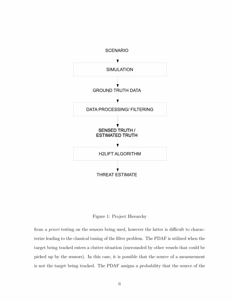
Figure 1: Project Hierarchy
from a priori testing on the sensors being used, however the latter is difficult to charac-
terize leading to the classical tuning of the filter problem. The PDAF is utilized when the
target being tracked enters a clutter situation (surrounded by other vessels that could be
picked up by the sensors). In this case, it is possible that the source of a measurement
is not the target being tracked. The PDAF assigns a probability that the source of the
ii

measurement is the target in track and utilizes this probability in its state estimates. The
Multiple-Model Adaptive Estimation algorithm (MMAE) is a technique utilizing parallel
EKF’s, each with a unique assumption of the unknown system parameters. The overall
estimate is a weighted sum of the individual filter estimates. The weights are determined
based on a pre-defined likelihood function and measurement residuals used to quantify
the relative correctness of each elemental estimate. The GMMAE is an improvement to
the traditional MMAE in that the GMMAE utilizes a bank of the n most recent mea-
surement residuals and an autocorrelation matrix rather than just the current residual.
Therefore a quicker filter convergence is realized.
iii

List of Variables
Table 1 summarizes the symbols used throughout this work.
Ts Sample Timek Time Sample Index, t = kTs, 1 ≤ k ≤ Kq Ship Index, 1 ≤ q ≤ Qλ LongitudeL Geocentric Latitude/ MMAE Likelihood Functionh Altitudeγ Flight Path AngleH Heading Angle (true course)/ Kalman Filter Measurement MatrixΩe Rate of Rotation of the Earthψ Euler Angle defining the alignment of the vehicle reference
x-axis with respect to the gravity x-axisΘ Euler Angle defining the alignment of the vehicle reference
y-axis with respect to the gravity y-axisφ Euler Angle defining the alignment of the vehicle reference
z-axis with respect to the gravity z-axisx State vectoru Input vectorW Process noiseν Measurement noisey Measurement vectorΦ Discrete time state transition matrixΓ Discrete time input distribution matrixυ Discrete time process noise distribution matrixP Covariance matrixK Kalman filter gain matrixR Sensor noise covarianceQ Process noise covarianceC Autocorrelation matrixw Weight matrixe Measurement residualǫ Bank of measurement residuals
Table 1: Symbols
iv

Notation
Table 2 summarizes the notation used throughout this work.
(. . .)− Discrete-time propogated value(. . .)+ Discrete-time updated value
ˆ(. . .) Estimated value˙(. . .) First derivative with respect to time¨(. . .) Second derivative with respect to time
+λ East Longitude−λ West Longitude+L North Latitude−L South Latitude
Table 2: Notation
Table of Abbreviations
Table 3 summarizes the abbreviations used throughout this work.
KF Linear Kalman FilterEKF Extended Kalman FilterMMAE Multiple-Model Adaptive EstimationGMMAE Generalized Multiple-Model Adaptive EstimationPDAF Probabalistic Data Association FilterGPS Global Positioning SystemINS Inertial Navigation System
Table 3: Table of Abbreviations
v

List of Figures
1 Project Hierarchy . . . . . . . . . . . . . . . . . . . . . . . . . . . . . . . ii
2.1 Geocentric vs. Geodetic Latitude . . . . . . . . . . . . . . . . . . . . . . 142.2 Sampling Frequency Greater Than Twice the Nyquist Frequency . . . . . 202.3 Sampling Frequency Less Than Twice the Nyquist Frequency . . . . . . . 202.4 Effects of Insufficient Sampling . . . . . . . . . . . . . . . . . . . . . . . 212.5 Probability Data Association Filter Methodology . . . . . . . . . . . . . 352.6 MMAE Framework . . . . . . . . . . . . . . . . . . . . . . . . . . . . . . 36
3.1 Navigation Methodology . . . . . . . . . . . . . . . . . . . . . . . . . . . 493.2 Longitude Conditioning . . . . . . . . . . . . . . . . . . . . . . . . . . . 513.3 Condition Ship Tracks . . . . . . . . . . . . . . . . . . . . . . . . . . . . 523.4 Ensuring Stall Time is While Ship is In Route . . . . . . . . . . . . . . . 54
4.1 Sample Ship Tracks with Constant Sample Time . . . . . . . . . . . . . . 614.2 Sample Ship Tracks with Varying Sample Time . . . . . . . . . . . . . . 624.3 Sample Velocities . . . . . . . . . . . . . . . . . . . . . . . . . . . . . . . 634.4 Rescue Helicopter . . . . . . . . . . . . . . . . . . . . . . . . . . . . . . . 664.5 Helicopter Velocities . . . . . . . . . . . . . . . . . . . . . . . . . . . . . 674.6 Helicopter Latitude and Longitude . . . . . . . . . . . . . . . . . . . . . 674.7 Ship Tracks for Scenario 3 . . . . . . . . . . . . . . . . . . . . . . . . . . 704.8 Ship Velocities for Scenario 3 . . . . . . . . . . . . . . . . . . . . . . . . 714.9 Helicopter Velocities for Scenario 3 . . . . . . . . . . . . . . . . . . . . . 714.10 Time Histories of Latitude and Longitude for Helicopters . . . . . . . . . 724.11 One Hundred Ship Scenario . . . . . . . . . . . . . . . . . . . . . . . . . 754.12 Convergence of GMMAE Weights for 40 Elements . . . . . . . . . . . . . 764.13 Simulation 1: Convergence of Probability Pd Estimate . . . . . . . . . . . 764.14 Simulation 1: Convergence of Probability Pq Estimate . . . . . . . . . . . 774.15 Simulation 1: Convergence of Latitudinal Process Noise Estimate . . . . 774.16 Simulation 1: Convergence of Longitudinal Process Noise Estimate . . . . 784.17 Simulation 1: Time History of Latitude and Longitude Tracking Errors . 794.18 Simulation 1: 3-Sigma Ellipses . . . . . . . . . . . . . . . . . . . . . . . . 794.19 Simulation 1: Time History of Data Association . . . . . . . . . . . . . . 804.20 Simulation 1: Tracking Performance with Calculated Estimates . . . . . 814.21 Gaussian distribution “Spread” . . . . . . . . . . . . . . . . . . . . . . . 814.22 Convergence of GMMAE Weights for 300 Elements . . . . . . . . . . . . 82
vi
4.23 Simulation 2: Convergence of PD Estimate . . . . . . . . . . . . . . . . . 834.24 Simulation 2: Convergence of PG Estimate . . . . . . . . . . . . . . . . . 844.25 Simulation 2: Convergence of qlat Estimate . . . . . . . . . . . . . . . . . 854.26 Simulation 2: Convergence of qlong Estimate . . . . . . . . . . . . . . . . 854.27 Simulation 2: Time History of Tracker Error with 3-Sigma Ellipses . . . . 864.28 Simulation 2: Tracker Error for 3 Estimates and Corresponding 3-Sigma
Ellipses . . . . . . . . . . . . . . . . . . . . . . . . . . . . . . . . . . . . 864.29 Simulation 2: Errors for Each Estimate and Largest 3-Sigma Ellipse . . . 874.30 Simulation 2: Time History of Data Association Probability . . . . . . . 87
5.1 Hammersley quasi-random sequence “spread” . . . . . . . . . . . . . . . 91
vii

List of Tables
1 Symbols . . . . . . . . . . . . . . . . . . . . . . . . . . . . . . . . . . . . iv2 Notation . . . . . . . . . . . . . . . . . . . . . . . . . . . . . . . . . . . . v3 Table of Abbreviations . . . . . . . . . . . . . . . . . . . . . . . . . . . . v
2.1 Spherical Earth Radius Options . . . . . . . . . . . . . . . . . . . . . . . 152.2 Linear Kalman Filter Equations . . . . . . . . . . . . . . . . . . . . . . . 262.3 Extended Kalman Filter Equations . . . . . . . . . . . . . . . . . . . . . 282.4 Probability Data Association Filter Equations . . . . . . . . . . . . . . . 342.5 Multiple-Model Adaptive Estimation Equations . . . . . . . . . . . . . . 392.6 Generalized Multiple-Model Adaptive Estimator Equations . . . . . . . . 42
3.1 Symbols Used in Flow Charts . . . . . . . . . . . . . . . . . . . . . . . . 483.2 Contextual Information Structure . . . . . . . . . . . . . . . . . . . . . . 57
4.1 Simulation Inputs for Scenario 1 . . . . . . . . . . . . . . . . . . . . . . . 604.2 Contextual Information Structure . . . . . . . . . . . . . . . . . . . . . . 644.3 Simulation Inputs for Scenario 2 . . . . . . . . . . . . . . . . . . . . . . . 654.4 Simulation Inputs for Scenario 3 . . . . . . . . . . . . . . . . . . . . . . . 694.5 Simulation Inputs for Scenario 4 . . . . . . . . . . . . . . . . . . . . . . . 734.6 Summary of Simulation Results . . . . . . . . . . . . . . . . . . . . . . . 83
viii

Chapter 1
Statement of Work and Literature
Review
1.1 Statement of Work
In this work, scenario simulations required for the H2LIFT project will be developed.
The simulator is developed in Matlab and is used to generate ground truth data for vessel
kinematics. The simulations will generate realistic data that subscribes to the laws of
physics, specific ship capabilities, and common maritime domain practices. Suspicious
maneuvers can either be randomly selected by the model or dictated by the user for each
simulation run. The simulation parameters are automatically adjusted according to these
variables ensuring unique and sensible scenario generations for each simulation run.
The simulation package also assigns a variety of contextual information including
nationalities, crew member information, float plans, etc. The simulation package includes
options for shipping route designation, flag changes, crew members on board (names,
ages, nationalities, etc).
The Generalized Multiple Model Adaptive Estimation (GMMAE) algorithm devel-
oped in Section 2.9 is used to tune a state estimator that was previously tuned by hand
1
in an ad-hoc process. The state estimator tracks the simulated ships from noisy mea-
surement signals and a system model.
1.2 Literature Review
A literary review was conducted recovering past research that would be of value to the
simulation and data processing/filtering stages of the H2LIFT project.
• Dr. Bjorkholm, Paul, “Optimizing a layered port security system”
http://www.porttechnology.org
This article discusses the combination of various security inspection technologies to
improve reliability and suggests that the manor in which the systems are combined
strongly affects the results achieved. Some examples of modern WMD detection
systems include portal monitors, gamma ray imagers, high-energy X-ray imagers,
and neutron systems. The way in which these technologies are combined or layered
depends on the particular goals of the system as a whole. For example, at one
extreme there is an arrangement in which all technologies are implemented one at
a time. The work suggests with this arrangement all the WMD threats passing
through the inspection will be detected, however the overall time the process con-
sumes is unreasonable and is detrimental to maritime commerce. Conversely, there
is an arrangement where only suspicious ships will be inspected. This arrangement
is very expeditious, however, it does not offer an acceptable level of security. This
article goes on to suggest various combinations of screening technologies in order to
achieve different results and explains the advantages and disadvantages of each ar-
rangement. The information is useful since insight into the probability of a positive
2
identification of a WMD on board a cargo ship is shown.
• Orphan, Victor. Muenchau, Ernie. Gormley, Jerry. and Richardson, Rex. “Ad-
vanced
Cargo Container Scanning Technology Development” Science Applications
International Corporation.
http://gulliver.trb.org/Conferences/MTS/3A%20Orphan%20Paper.pdf
This paper describes the methods of detecting terrorist threats in cargo contain-
ers. Such methods include Mobile VACIS, Portal VACIS, Radiation Scanning,
Automated Vehicle and Container Identification, Material Specific Scanning using
Neutron Interrogation, Integrated Display (ICIS Viewer), and Automatic Empty
Container Verification System. The paper describes each method and demonstrates
the need for an Integrated Container Inspection System (ICIS). This paper is im-
portant because it gives insight into the United States technological capabilities.
• Dr. Purdy, Caroline. “Detection Systems for Radiological and Nuclear Counter-
measure (DSRNC)” DHS Intramural Laboratories. February 18, 2004
http://www.iwar.org.uk/news-archive/conference/dhs-dsrnc.pdf
This presentation describes some current research regarding detection systems for
radiological and nuclear countermeasure. The technologies include: Real-time mul-
tiplicity counter and fission meter, Adaptable Radiation Area Monitor, Gamma-ray
Imaging Spectrometer, SMART Detector System, SmartCart System, Sensor Man-
agement Architecture, Intelligent Sensing Modules, PAKTRAK, Highly Portable
Large-Area Sensors, Multicoincedence Analysis Methods, Scenario Analysis Meth-
ods, etc. . . This paper is important because it gives insight into the United States
3
technological capabilities.
• “Smart Buoys Help Protect Submarine Base” Defense Threat Reduction Agency.
Lawrence Livermore National Laboratory. 2004.
http://www.llnl.gov/str/JanFeb04/Valentine.html
This article briefs the implementation of buoys outfitted with commercially avail-
able radiation detectors. The first two buoys were installed at the U.S. Navy’s
submarine base at Kings Bay, Georgia. The article explains the idea behind the
buoys and suggests that if the two at Kings Bay are successful the technology will
be implemented at civilian areas such as busy ports. The information is valuable
because it gives insight into the future of maritime domain awareness.
• Thomas, Guy. “A Maritime Traffic-Tracking System: Cornerstone of Maritime
Homeland Defense” 6/12/2006.
http://www.nwc.navy.mil/press/Review/2003/Autumn/rd1-a03.htm
This article argues that the United States should track and identify every ship,
along with its cargo, crew, and passengers, well before any vessel or cargo enter
any of the country’s ports or pass near anything of value to the United States.
This is a controversial topic because some people believe that it would be far too
difficult or not worthwhile to implement such a system. This article discusses this
issue in detail and strongly supports the implementation of such a system as well
as suggests specific methods. It is important to the H2LIFT project because it
gives insight into an optional direction for the U.S. to secure the border.
• “WMD Hunting Technology” Williamson Labs, 2004.
http://www.williamson-labs.com/cbr-tech.htm
4

This article describes the various technologies available for detecting weapons of
mass destruction, the factors influencing the successful detection of nuclear ma-
terials (Intensity of source, distance from sensor, shielding, background radiation,
detector types, and exposure time), and features that can improve the detection
of nuclear materials (Selectivity, Directivity, and Radiography). This article gives
some insight into some variables that can be built into the H2LIFT simulations to
influence the WMD detection.
• Thomas, Guy. “Capabilities and Systems for Maritime Domain Awareness”, 6/12/2006.
http://www.nwc.navy.mil/press/Review/2003/Autumn/rd1-app-a03.htm
This article describes the currently capabilities of identifying ships and cargo. Such
methods described include: Maritime Mobile Service identifier (MMSI), Automatic
Identification System, Digital Selective Calling, Commercial Satellite Communica-
tions Systems, and Container Tracking Systems. The article also discusses Multi-
level security, Area Security Operations Command and Control, and Smart Agents.
This article is important because it gives insight into the technologies available, and
those currently in use, to increase maritime domain awareness.
• “Radar” Wikipedia, the free encyclopedia. 6/6/2006.
http://en.wikipedia.org/wiki/Radar
This is the Wikipedia Encyclopedias definition of Radar. Briefly, radar is a system
that uses radio waves to detect (determine the distance or speed) objects such as
aircraft, ships, and rain and map them. Speed is determined by the amount of
Doppler effect frequency shift of the reflected signal. The article describes ways
in which radar can be blocked using radar-absorbing materials or materials that
reflect radar in a direction other than back to the receptors and various forms of
5
interference experienced when using radar (noise, clutter, Jamming, etc. . . ). The
article is useful because it gives insight into the accuracy of radar measurements.
• “Transponder Tracking For Cargo Ships” Navy League of the United States. Au-
gust 2005.
http://www.navyleague.ort/sea power/aug 05 05.php
This article suggests a method that uses transponders to track cargo ships. The
article states that the U.S. should insist any ship wanting access to any U.S. port
be equipped with a transponder that is continuously transmitting an identification
signal specific to that vessel. The transponder would be manufactured and pro-
grammed in the U.S. and sealed with build-in self-destruct if opened or removed
from the vessel assigned. The article also suggests methods to make use of cur-
rent technologies to implement this mandatory transponder tracking. The article
is important because it gives insight into the future of maritime domain awareness
techniques.
• “Global Positioning System” Wikipedia, the free encyclopedia.
6/6/2006. http://en.wikipedia.org/wiki/Gps
This is the Wikipedia Encyclopedias definition of Global Positioning System (GPS).
It discusses the history, technical description, problems, alternatives, and Military/
civilian applications of GPS and explains the GPS available to civilians is limited
compared to the actual capabilities of GPS in order to prevent its use in missile
guidance and other terrorist applications. It is useful because it provides insight
6

into the accuracy of GPS measurements.
• “GPS System Description” United States Naval Observatory (USNO) 6/6/2006.
ftp://tycho.usno.navy.mil/pub/gps/gpssy.txt
This paper describes the capabilities of GPS, system segments, selective availability
and anti-spoofing, system time, and time transfer. It explains the two levels of
GPS service: The Standard Positioning Service (SPS) and the Precise Positioning
Service (PPS). The SPS is available to all GPS users on a continuous, worldwide
basis with no direct charge. The PPS is a more accurate positioning, velocity
and timing service which is available on a continuous, worldwide basis only to users
authorized by the U.S. This gives some insight into the technology available to track
vessels. Although GPS is not commonly used in modern ship tracking methods, it
is an option for the future.
• Clynch, James R.,“Geodetic Coordinate Conversions”, 2002
http://www.oc.nps.navy.mil/oc2902w/coord/coordcvt.pdf
This article presents the conversion between Geodetic and Geocentric Latitudes,
and from Latitude, Longitude, Height coordinates to ECEF (Earth Centered, Earth
Fixed) coordinates and provides the equations required to perform the conversions.
The article is primarily used to develop the equations-of-motion required for the
simulation package.
• Clynch, James R.,“Radius of Earth - Radii used on Geodesy”, 2002
http://www.oc.nps.navy.mil/oc2902w/geodesy/radiigeo.pdf
This article introduces radii concepts used on Geodesy. In general there are three
radii that are a function of latitude in the ellipsoidal model of the earth:
7
1. The physical radius: the distance from the center of the earth to the ellipsoid
surface.
2. Radius of curvature in the Prime Vertical.
3. Radius of curvature in the meridian.
The article gives details of each radii and reveals a general mathematical formula
to describe them. This article provides insight into a method for developing an
accurate earth model.
• Dr. Mason, Paul A.C., and Walchko, Kevin J.,“Inertial Navigation”, 2002
http://www.mil.ufl.edu/publications/fcrar02/
walchko inertial navigation fcrar 02.pdf
This paper discusses the design and implementation of an Inertial Navigation Sys-
tem (INS) using an Inertial Measurement Unit (IMU) and Global Positioning Sys-
tem (GPS). This article is important to the simulation package because it provides
a derivation of the equations used to convert from Inertial Measurement Units to
Latitude and Longitude coordinates.
• Williams, Edward, “Aviation Formulary V1.42”, 6/15/2006
http://williams.best.vwh.net/avform.htm
The purpose of this article is to serve as an introduction to great circle navigation
and how to compute courses, headings, and other navigational quantities of inter-
est using a spherical earth model. A shortcoming of great circle navigation is it
involves a continuously changing heading angle (true course). Navigating between
two points on the Earths surface using a route of constant heading angle is possible
through Rhumb Line navigation. This article derives and describes the formulas
8
used in great circle navigation on a spherical earth. It will be useful as a possible
method for computing courses and headings for the H2LIFT simulation package.
• Williams, Edward, “Rhumb Lines”, 2006
http://williams.best.vwh.net/ellipsoid/node3.html
This article serves as an introduction to Rhumb Line navigation and how to com-
pute courses, headings, and other navigational quantities of interest. It derives
and explains the formulas used in Rhumb line navigation, which involves routes of
constant heading angle (true course). This information will be useful as a possible
method for computing courses and headings for the H2LIFT simulation package.
• Crassidis, J.L., and Cheng, Y., “Generalized Multiple-Model Adaptive Estimation
Using an Autocorrelation Approach,” 9th International Conference on Information
Fusion, Florence, Italy, July 2006, paper 223.
This paper introduces a new adaptive law for the traditional MMAE algorithms to
be used in estimating unknown noise statistics in filter design. The new adaptive
law is based on autocorrelation of the measurement-minus-estimate residual. The
proposed algorithm utilizes a bank of such residuals (containing residuals of past
measurements) while the traditional MMAE algorithms depend only on the cur-
rent measurements residual. The new law is shown to provide better convergence
properties than the traditional MMAE algorithms. This information is useful in
that it provides insight into recent research in estimation algorithms.
• Crassidis, J.L., and Junkins, J.L., Optimal Estimation of Dynamic Systems, Chap-
man & Hall/CRC Press, Boca Raton, FL, 2004. p. 285-292.
9

This text introduces estimation techniques and provides derivations of the Kalman
filter equations in its various forms (Continuous, Discrete, Continuous-Discrete, Ex-
tended, etc). It also provides a review of mathematical techniques and probability
concepts necessary for understanding the nature of estimation techniques.
• P.D. Hanlon and P.S. Maybeck, “Multiple-Model Adaptive Estimation using a
Residual Correlation Kalman Filter Bank,” IEEE Transactions on Aerospace and
Electronic Systems, Vol. AES-36, No. 2, April 2000, pp.393-406.
This paper gives an overview of the traditional MMAE algorithm and proposes a
modification for use with detection of flight control actuator failures. In order to
detect an actuator failure, one must continuously excite the actuators and analyze
the output. The constant excitation of the actuators may be objectionable to the
aircraft pilot and passengers. The proposed MMAE algorithm adjustment allows
a significant reduction in the amplitude of the system dither inputs used to excite
the system modes making the process less objectionable. This information is useful
in that it provides insight into recent research in estimation algorithms.
• C.D. Ormsby, Dissertation: “Generalized Residual Multiple Model Adaptive Esti-
mation of Parameters and States.” Air Force Institute of Technology. October 2003
This dissertation demonstrates some active work in the area of MMAE algorithms.
Specifically, the author proposes a modification to the traditional MMAE algorithm
in which he makes use of a “generalized residual.” This new residual is a linear
combination of traditional Kalman filter residuals and the residuals after the mea-
surement has been incorporated. The author also introduces different techniques
used to address specific problems that arise in MMAE algorithms. Such techniques
include β-stripping, probability lower bounding, etc. This information is useful in
10

that it provides insight into recent research in estimation algorithms.
11
Chapter 2
Theory and Supporting Material
2.1 Reference Frames
In this section, reference frames for the Global Positioning System (GPS) and Inertial
Navigation System (INS) applications are presented:
• Earth-Centered-Inertial (ECI): A right-handed coordinate system denoted by ı1,
ı2, ı3. The ı1 axis is directed towards the vernal equinox, the ı3 axis is directed
toward the North pole, and the ı2 axis follows the rules of a right handed coordinate
system. Note that the ECI frame does not rotate with respect to the stars (except
for procession of equinoxes) and the Earth turns relative to this frame. Vectors
described using ECI coordinates are denoted by a superscript I [5].
• Earth-Centered-Earth-Fixed (ECEF): A right-handed coordinate system denoted
by e1, e2, e3. This frame is similar to the ECI frame with e3 = ı3; however, the
e1 axis is directed towards the Earth’s prime meridian, and the e2 axis completes
the right hand coordinate system. Note, the ECEF frame rotates with the Earth.
Vectors described using ECEF coordinates are denoted by a superscript E [5].
• North-East-Down (NED): A right-handed coordinate system denoted by n, e, d.
The n axis is directed north, the e axis is directed east, and the d axis completes
12
the right- handed coordinate system (pointing towards the center of the earth on a
spherical earth model) [5]. Note, the plane formed by the n and e axes is tangent to
the Earths surface with the d axis perpendicular to the Earth’s surface. Therefore,
the axis system is convenient for local navigation purposes. Vectors described using
NED coordinates are denoted by a superscript N in this work.
• Gravity Axes: A right-handed coordinate system denoted by Xg, Yg, Zg. The Zg
axis is directed towards the Earth’s center, Yg is directed towards the south pole,
and Xg completes the right-hand system by pointing East [5]. Note, similar to the
NED coordinates, this coordinate system is based at the Earth’s surface.
2.2 Geodetic vs. Geocentric Latitude
Figure 2.1 displays the distinction between Geodetic and Geocentric Latitude. The angle
L’ is “geocentric latitude” and is defined as the angle between the equatorial plane and
the radius from the Earth’s geocenter. The angle L is “geodetic latitude” and is defined
as the angle between the equatorial plane and the normal to the surface of the ellipsoid
[6]. The word “latitude” typically refers to geodetic latitude, and is the basis for most
maps and charts. Note, for a spherical earth model there is no differentiating between
geocentric latitude and geodetic latitude.
2.3 Earth Modeling
This section presents three basic types of Earth models commonly used for describing
motion relative to the fixed Earth frame differing in their assumption of the Earth’s
shape. The models are introduced in order of increasing accuracy.
Flat Earth: These models are used for plane surveying over distances short enough so
that the Earth’s curvature is insignificant (less than 10 km) [6]. These models are increas-
13

Figure 2.1: Geocentric vs. Geodetic Latitude
14
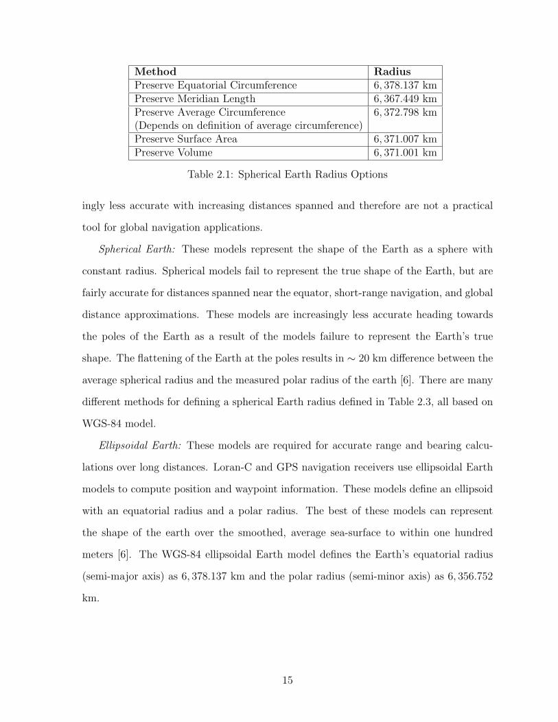
Method RadiusPreserve Equatorial Circumference 6, 378.137 kmPreserve Meridian Length 6, 367.449 kmPreserve Average Circumference 6, 372.798 km(Depends on definition of average circumference)Preserve Surface Area 6, 371.007 kmPreserve Volume 6, 371.001 km
Table 2.1: Spherical Earth Radius Options
ingly less accurate with increasing distances spanned and therefore are not a practical
tool for global navigation applications.
Spherical Earth: These models represent the shape of the Earth as a sphere with
constant radius. Spherical models fail to represent the true shape of the Earth, but are
fairly accurate for distances spanned near the equator, short-range navigation, and global
distance approximations. These models are increasingly less accurate heading towards
the poles of the Earth as a result of the models failure to represent the Earth’s true
shape. The flattening of the Earth at the poles results in ∼ 20 km difference between the
average spherical radius and the measured polar radius of the earth [6]. There are many
different methods for defining a spherical Earth radius defined in Table 2.3, all based on
WGS-84 model.
Ellipsoidal Earth: These models are required for accurate range and bearing calcu-
lations over long distances. Loran-C and GPS navigation receivers use ellipsoidal Earth
models to compute position and waypoint information. These models define an ellipsoid
with an equatorial radius and a polar radius. The best of these models can represent
the shape of the earth over the smoothed, average sea-surface to within one hundred
meters [6]. The WGS-84 ellipsoidal Earth model defines the Earth’s equatorial radius
(semi-major axis) as 6, 378.137 km and the polar radius (semi-minor axis) as 6, 356.752
km.
15

2.4 Navigation
This section introduces the method of great circle navigation and details of rhumb line
navigation. Rhumb line navigation is the route calculation method of choice for the
H2LIFT project. Note, this work uses the convention Western longitudes and Southern
latitudes are represented as negative while Eastern longitudes and Northern latitudes are
positive. i.e. − latitude and longitude denotes South and West respectively, while +
latitude and longitude denotes North and East respectively.
2.4.1 Great Circle Navigation
The shortest distance between two locations on the Earth’s surface is a straight line
slicing through the Earth. Obviously, not a realistic option when deciding transportation
routes. The shortest distance following the Earth’s surface (i.e. that can be realistically
traversed) inherently lies vertically above the aforementioned straight-line route and gives
rise to the concept of great circle navigation. Conceptually, the construction of a great
circle route involves creating an imaginary plane that intersects the two points of interest
as well as the center of the earth. The plane slices the (assumed spherical) Earth into
2 hemispheres of equal size. The circumference of the flat face of each hemisphere is
referred to as a great circle [12]. Note, only planes slicing through the center of the earth
give rise to great circles, i.e., all meridians are great circles, while the equator is the only
line of latitude known as a great circle.
2.4.2 Rhumb Line Navigation
A shortcoming of great circle navigation is the heading angle varies continuously. For
example, the great circle route between two points of equal (non-zero) latitude does not
follow the line of latitude in an E-W direction, instead it arcs towards the pole. However,
it is possible to traverse two points using a constant heading angle by using the method
16
of rhumb line navigation [13]. Note, an aircraft flying a great circle route for a sufficient
amount of time would encircle the earth and return to the original starting point, while
an aircraft flying a rhumb line route would spiral indefinitely poleward. A great circle
route between two points of equal longitude, or of zero latitude is equivelant to the rhumb
line route between the same two points.
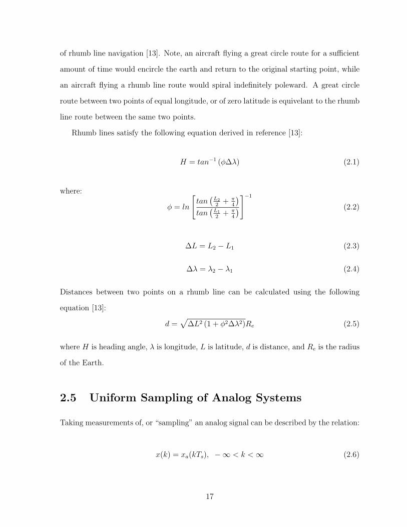
Rhumb lines satisfy the following equation derived in reference [13]:
H = tan−1 (φ∆λ) (2.1)
where:
φ = ln
[
tan(
L2
2+ π
4
)
tan(
L1
2+ π
4
)
]−1
(2.2)
∆L = L2 − L1 (2.3)
∆λ = λ2 − λ1 (2.4)
Distances between two points on a rhumb line can be calculated using the following
equation [13]:
d =√
∆L2 (1 + φ2∆λ2)Re (2.5)
where H is heading angle, λ is longitude, L is latitude, d is distance, and Re is the radius
of the Earth.
2.5 Uniform Sampling of Analog Systems
Taking measurements of, or “sampling” an analog signal can be described by the relation:
x(k) = xa(kTs), −∞ < k <∞ (2.6)
17
where x(k) is the discrete-time signal obtained by sampling the analog signal xa(t) every
Ts seconds. Ts is the uniform time interval between samples, or sampling interval, and
its inverse is the sampling frequency, 1Ts
= Fs.
With uniform sampling, there is a linear relationship between t of the analog signal
and k of the discrete-time signal written as:
t = kTs =k
Fs
(2.7)
As a consequence of eqn.(2.7) there exists a relationship between the frequency variable
F for analog signals and the frequency variable f for discrete signals [11]. To establish
the relationship, consider an analog sinusoidal signal of the form:
xa(t) = cos(2πFt) (2.8)
that will be sampled to obtain a digital sinusiod of the form:
x(k) = cos(2πfk) (2.9)
To “sample” the analog signal uniformly at a rate of Fs = 1Ts
Hz, substitute kT or kFs
in
for t in eqn.(2.8):
xa(kT ) = x(k) = cos(2πFkT ) = cos
(
2πF
Fs
k
)
(2.10)
Comparing eqns.(2.9) and (2.10) reveals the frequency relation as:
f =F
Fs
(2.11)
Note, from reference [11], the range of frequencies for analog sinusoids is:
−∞ < F <∞ (2.12)
18
However, the range for discrete time sinusoids is:
−1
2< f <
1
2(2.13)
Substituting eqn.(2.11) into eqn.(2.13) results in:
−Fs
2≤ F ≤ Fs
2(2.14)
This means that the highest frequency that can be uniquely distinguished from the digital
signal is:
Fmax =Fs
2(2.15)
i.e., in order to fully represent the frequency content of the analog signal with a digital
signal, it must be sampled at least twice as fast as the highest frequency present in the
analog signal. Fmax in eqn.(2.15) is known as the “Nyquist frequency.” Sampling at
any rate less than twice the Nyquist frequency will result in aliasing, or the inability to
accurately recreate the analog signal from its resulting digital representation. Figure 2.2,
2.3, and 2.4 demonstrate this effect.
Note, from Figure 2.2, the analog frequency of 0.5 Hz is preserved in the reconstructed
signal because the sampling rate is greater than twice the Nyquist frequency. However,
from Figure 2.3, the analog frequency appears to be just slightly faster than f = 1cycle
8seconds=
0.125 Hz. If the frequency content of the analog signal is not known prior to sampling,
an inappropriate sampling frequency can be used causing aliasing without any indication
that it is occuring.
The H2LIFT simulation package is simulating a continuous scenario with a digital
computer. When generating ground truth, it must be assured that a fast enough sampling
rate is used such that all of the interesting events are represented by the digital simulation.
For instance, in Figure 2.4, say the extrema of the analog function are analogous to
interesting or eratic behavior of a ship in a maritime scenario and the X ′s represent
19

0 2 4 6 8 10 12−1
−0.5
0
0.5
1Sampling Rate > Nyquist
x a(t)
and
x a(nT
)
0 2 4 6 8 10 12−1
−0.5
0
0.5
1
Rec
reat
ion
of x
a(t)
from
xa(n
T)
t, and nT
Figure 2.2: Sampling Frequency Greater Than Twice the Nyquist Frequency
0 2 4 6 8 10 12−1
−0.5
0
0.5
1Sampling Rate < Nyquist
x a(t)
and
x a(nT
)
0 2 4 6 8 10 12−1
−0.5
0
0.5
1
Rec
reat
ion
of x
a(t)
from
xa(n
T)
t, and nT
Figure 2.3: Sampling Frequency Less Than Twice the Nyquist Frequency
20
0 5 10 15 20 25
−2
−1
0
1
2
f(x)
Continuous Function
0 5 10 15 20 25
−2
−1
0
1
2
f(x)
Sampled Function
x
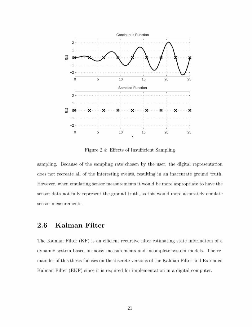
Figure 2.4: Effects of Insufficient Sampling
sampling. Because of the sampling rate chosen by the user, the digital representation
does not recreate all of the interesting events, resulting in an inaccurate ground truth.
However, when emulating sensor measurements it would be more appropriate to have the
sensor data not fully represent the ground truth, as this would more accurately emulate
sensor measurements.
2.6 Kalman Filter
The Kalman Filter (KF) is an efficient recursive filter estimating state information of a
dynamic system based on noisy measurements and incomplete system models. The re-
mainder of this thesis focuses on the discrete versions of the Kalman Filter and Extended
Kalman Filter (EKF) since it is required for implementation in a digital computer.
21
2.6.1 Linear
The discrete-time linear Kalman filter can be applied when the system model is linear
and both the system model and sensor measurements are available in discrete-time form.
Process noise is added to the system model accounting for modeling inaccuracies and
sensor noise is inherent to any measurement process. The following derivation is based
on reference [4]. The linear model is defined as:
xk+1 = Φxk + Γuk + Υwk (2.16)
y = Hxk + νk (2.17)
Where x is the state vector, Φ is the state transition matrix, Γ is the input distribu-
tion matrix, u is the input vector, Υ is the process noise distribution matrix, y is the
measurement vector, H is the measurement matrix, w is the process noise, and ν is the
sensor noise. The noise is assumed to be zero-mean Gaussian white-noise. The constraint
implies the noise is not correlated forward or backward in time or with each other such
that:
EνkνTj =
0 k 6= j
Rk k = j(2.18)
EwkwTj =
0 k 6= j
Qk k = j(2.19)
EνkwTk = 0,∀ k (2.20)
where the E operator denotes the expectation, and R and Q are the sensor noise and
process noise covariances respectively. In practice, Rk is known approximately from a
22

priori tests and knowledge of the sensors being used, while Qk is unknown and difficult
to characterize. Methods for approximating Qk and other unknown parameters are in-
troduced in Sections 2.8 and 2.9.
The current state estimate is based on the current measurement and model, and is
accomplished by feeding back the difference between the measured and estimated output.
Thus the form of the estimate is:
x−k+1 = Φx+k + Γuk (2.21)
x+k = x−k +Kk[yk −Hx−k ] (2.22)
where x denotes the estimate of x, superscript − denotes the propogated value, superscript
+ denotes the updated value, and K is the Kalman filter gain. The error covariances are
defined by:
P−k ≡ Ex−k x−T
k , P−k+1 ≡ Ex−k+1x
−Tk+1
P+k ≡ Ex+
k x+Tk , P+
k+1 ≡ Ex+k+1x
+Tk+1
(2.23)
where the state errors in the prediction and update are:
x−k ≡ x−k − xk, x−k+1 ≡ x−k+1 − xk+1
x+k ≡ x+
k − xk, x+k+1 ≡ x+
k+1 − xk+1
(2.24)
Assuming the initial conditions of the states are known, the following initializations hold
true:
x(t0) = x0 (2.25)
P0 = Ex0xT0 (2.26)
23
Expressions for both P−k+1, P
+k and an optimal gain Kk must be derived to complete the
Kalman filter equations. P−k+1 can be found by substituting eqn.(2.16) and (2.21) into
(2.24) and results in:
x−k+1 = Φx+k −Υkwk (2.27)
Thus:
P−k+1 ≡ Ex−k+1x
−Tk+1 =
= EΦx+k x
+Tk ΦT − EΦx+
k wTk ΥT
k −
− EΥkwkx+Tk ΦT
k + EΥkwkwTk ΥT
k (2.28)
From eqn.(2.16) it is apparent that wk and x+k are uncorrelated since x+
k+1 (not x+k )
directly depends on wk. Thus Ex+k w
Tk = Ewkx
+Tk = 0. Using the definitions in
eqns.(2.18) and (2.23), eqn.(2.28) reduces to:
P−k+1 = ΦkP
+k ΦT
k + ΥkQkΥTk (2.29)
For P+k , substituting eqn.(2.17) into (2.22) and substituting the result into eqn.(2.24)
results in:
x+k = (I −KkHk)x−k +Kkνk (2.30)
Thus:
P+k ≡ Ex+
k x+Tk =
= E(I −KkHk)x−k x−Tk (I −KkHk)T+
+ E(I −KkHk)x−k νTk K
Tk +
24
+ EKkνkx−Tk (I −KkHk)T+ EKkνkν
Tk K
Tk (2.31)
From eqn.(2.22) it is clear that νk and x+k are uncorrelated since x+
k (not x−k ) directly de-
pends on νk. Therefore Ex−k νTk = Eνkx
−Tk = 0 and using the definition in eqns.(2.18)
and (2.23) eqn.(2.31) reduces to:
P+k = [I −KkHk]P−
k [I −KkHk]T +KkRkKTk (2.32)
Minimizing the length of the estimation error vector by minimizing the trace of P+k and
solving for the gain Kk results in:
Kk = P−k H
Tk [HkP
−k H
Tk +Rk]−1 (2.33)
Substituting eqn.(2.33) into eqn.(2.32) and simplifying results in:
P+k = [I −KkHk]P−
k (2.34)
The discrete-linear Kalman filter equations are summarized in Table 2.2. These equations
are used recursively with the starting point differing depending on the availability of a
measurement at k = 0. Specifically, if there is a measurement available at k = 0, then
the initial conditions serve as the propagated state and covariance estimates which are
updated based on the measurement via the update equations, i.e., eqns.(2.22) and (2.34)
are used with x−k = x0 and P−k = P0. Then, these updated estimates are propagated
to the next measurement using eqns.(2.21) and (2.29) where the process is repeated
for the new updated estimates for as long as measurements exist. However, if there
is not a measurement available at k = 0, the initial conditions serve as the updated
25
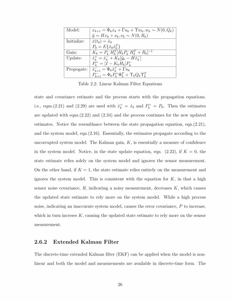
Model: xk+1 = Φkxk + Γuk + Υwk, wk ∼ N(0, Qk)y = Hxk + νk, νk ∼ N(0, Rk)
Initialize: x(t0) = x0
P0 = Ex0xT0
Gain: Kk = P−k H
Tk [HkP
−k H
Tk +Rk]−1
Update: x+k = x−k +Kk[yk −Hx−k ]P+
k = [I −KkHk]P−k
Propogate: x−k+1 = Φkx+k + Γuk
P−k+1 = ΦkP
+k ΦT
k + ΥkQkΥTk
Table 2.2: Linear Kalman Filter Equations
state and covariance estimate and the process starts with the propagation equations.
i.e., eqns.(2.21) and (2.29) are used with x+k = x0 and P+
k = P0. Then the estimates
are updated with eqns.(2.22) and (2.34) and the process continues for the new updated
estimates. Notice the resemblance between the state propagation equation, eqn.(2.21),
and the system model, eqn.(2.16). Essentially, the estimates propagate according to the
uncorrupted system model. The Kalman gain, K, is essentially a measure of confidence
in the system model. Notice, in the state update equation, eqn. (2.22), if K = 0, the
state estimate relies solely on the system model and ignores the sensor measurement.
On the other hand, if K = 1, the state estimate relies entirely on the measurement and
ignores the system model. This is consistent with the equation for K, in that a high
sensor noise covariance, R, indicating a noisy measurement, decreases K, which causes
the updated state estimate to rely more on the system model. While a high process
noise, indicating an inaccurate system model, causes the error covariance, P to increase,
which in turn increses K, causing the updated state estimate to rely more on the sensor
measurement.
2.6.2 Extended Kalman Filter
The discrete-time extended Kalman filter (EKF) can be applied when the model is non-
linear and both the model and measurements are available in discrete-time form. The
26
following model is used for the EKF:
xk+1 = f(xk, uk, k) + Υkwk (2.35)
yk = h(xk, k) + νk (2.36)
Similar to the linear case, νk and wk are the measurement and process noises, respectively.
Both are assumed to be zero-mean Gaussian white-noise processes so eqns.(2.18), (2.19),
and (2.20) apply. As with the linear KF, Rk is typically known while Qk is unknown
and difficult to characterize. The fundamental concept of the EKF is based on the
assumption that the true state is sufficiently close to the estimated state. In this context
sufficiently close means close enough to be accurately represented by a first-order Taylor
series expansion [4]. Consider the first-order expansion of the model and measurement
about some nominal state x(t):
f(xk, uk, k) ∼= f(xk, uk, k) +∂f
∂xxk
[xk − xk] (2.37)
h(xk, k) ∼= h(xk, k) +∂h
∂xxk
[xk − xk] (2.38)
Substituting the current estimate for the nominal state estimate (xk = xk) and taking
the expectation of both sides of eqns.(2.37) and (2.38) gives:
Ef(xk, uk, k) = f(xk, uk, k) (2.39)
Eh(xk, k) = h(xk, k) (2.40)
Therefore the estimator is of the form:
xk = f(xk, uk, k) +Kk[yk − h(xk, k)] (2.41)
27
Model: xk+1 = f(xk, uk, k) + Υkwk, wk ∼ N(0, Qk)yk = h(xk, uk, k) + νk, νk ∼ N(0, Rk)
Initialize: x(t0) = x0
P0 = Ex0xT0
Gain: Kk = P−k H
Tk (xk)[Hk(xk)P−
k HTk (xk) +Rk]−1
Where:H(xk, k) ≡ ∂h
∂x xk
Update: x+k = x−k +Kk[yk − h(xk, uk, k)]P+
k = [I −KkHk(xk)]P−k
Propogate: x−k+1 = f(x+k , uk, k)
P−k+1 = Fk(x+
k , k)P+k F
Tk (x+
k , k) + ΥkQkΥTk
Where:
F (xk, k) ≡ ∂f
∂x xk
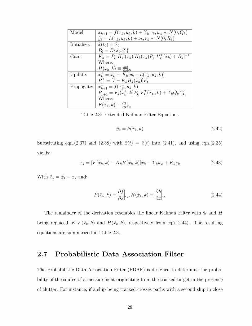
Table 2.3: Extended Kalman Filter Equations
yk = h(xk, k) (2.42)
Substituting eqn.(2.37) and (2.38) with x(t) = x(t) into (2.41), and using eqn.(2.35)
yields:
xk = [F (xk, k)−KkH(xk, k)]xk −Υkwk +Kkνk (2.43)
With xk = xk − xk and:
F (xk, k) ≡ ∂f
∂xxk, H(xk, k) ≡ ∂h
∂xxk
(2.44)
The remainder of the derivation resembles the linear Kalman Filter with Φ and H
being replaced by F (xk, k) and H(xk, k), respectively from eqn.(2.44). The resulting
equations are summarized in Table 2.3.
2.7 Probabilistic Data Association Filter
The Probabilistic Data Association Filter (PDAF) is designed to determine the proba-
bility of the source of a measurement originating from the tracked target in the presence
of clutter. For instance, if a ship being tracked crosses paths with a second ship in close
28
proximity, it is necessary to know the source of each measurement so the state estimates
are not updated based on a stray measurement. The following derivation is influenced
by reference [1].
In order to derive the PDAF it must be assumed that:
• Undesirable measurements (those that don’t originate from the target being tracked)
occur independently in time and space, therefore, inferences of the location, nature,
or number of future undesirable measurements cannot be made from past data.
• System Model (dynamics) and the covariance of the driving noise is known.
The PDAF uses all of the measurements possibly originating from the object in track
(i.e. all validated measurements) and makes use of the a posteriori probability that each
of the validated measurements in fact originated from this object. The feature of using all
of the validated measurements distinguishes the PDAF from previous approaches where
only a single measurement was deemed correct.
Incoming measurements must first satisfy a defined validation criterion before being
considered for updating a specific track. An advantage is gained since the procedure
greatly decreases the computational load of the algorithm. The residual, or innovation,
corresponding to the correct measurement (denoted by zk,i) is defined as:
zk,i , zk,i − z−k (2.45)
where z−k is the conditional mean of the observation and is assumed to be normally
distributed with zero mean. The covariance, Sk, of z−k is given by:
Sk = HkP−k H
Tk +Rk (2.46)
29

where:
P−k = ΦP+
k−1ΦT +Qk (2.47)
The validation test can be written as follows:
pk(zk,i) ≤ γ (2.48)
where γ is the validation threshold, zk,i denotes the innovation corresponding to the
measurement zk,i, and
pk(zk,i) , zTk,iS
−1k zk,i (2.49)
Substituting eqn.(2.45) into (2.49) and that result into eqn.(2.48), the validation test
becomes:
(zk − z−k )TS−1k (zk − z−k ) ≤ γ (2.50)
Let the validated measurements be denoted as:
Zk = zk,imk
i=1 (2.51)
and,
Zk , Zjkj=1 (2.52)
Thus, the minimum variance estimate is:
x+k =
∫
xkP (xk | Zk)dxk (2.53)
eqn.(2.53) is the mathematical basis for the PDAF algorithm.
Define the following events:
χk,i = zk,i is the correct measurement i = 1, . . . ,mk (2.54)
30
χk,0 = none of the validated measurements are correct (2.55)
Since only one measurement can be correct, the above events are mutually exclusive and
exhaustive (important for later developments). Now eqn.(2.53) can be written as:
x+k , Exk | Zk =
mk∑
i=0
Exk | χk,i, ZkPχk,i | Zk (2.56)
Next, the a posteriori probability of each measurement having originated from the
object being tracked (the probabalistic data association) is defined as:
βk,i , Pχk,i | Zk, i = 0, . . . ,mk (2.57)
Assume the following:
• The probability density of a correct measurement conditioned upon past data is:
p(zk,i | χk,i, Zk−1) , f(zk,i | Zk−1) (2.58)
• The density of an incorrect measurement is uniform in the validation region, whose
volume is denoted by Vk.
p(zk,i | χk,j, Zk−1) = V −1
k , j 6= i (2.59)
Based on the assumptions in eqns.(2.58) and (2.59), the a posteriori probability the
ith measurement is correct (from eqn.(2.57)) is obtained as:
βk,i =
f(zk,i | Zk−1)[
bk +
mk∑
i=1
f(zk,i | Zk−1)
]
, i = 1, . . . ,mk (2.60)
31

where,
bk , mkV−1k
PG + PD − PGPD
(1− PG)(1− PD)(2.61)
PG represents the probability the correct measurement will not lie in the validation region
and PD represents the probability the correct measurement will not be detected.
The a posteriori probability corresponding to none of the measurements being correct
(from eqn.(2.57)) is:
βk,0 =bk
[
bk +
mk∑
i=1
f(zk,i | Zk−i)
] (2.62)
eqns.(2.60) and (2.62) can be rewritten as:
βk,i =
c 1√|2πSk|
× exp−(zk,i)T S−1
kzk,i i = 1, . . . ,mk
c (1−PDPG)mk
PDVi = 0
(2.63)
eqn.(2.63) forms the PDA method. The approximate sufficient statistic of the past mea-
surement is denoted as:
Y −k = Px−k , P−
k (2.64)
From eqns.(2.45) through (2.49) the probability density of a measurement, given that
it originated from an object track and has been validated conditioned upon Zk−1 is a
truncated normal density.
f(zk,i | Y −k ) = (1− PG)−1N(Hkx
−k , Sk) (2.65)
Since the events χk,i for i, . . . ,mk defined in eqns.(2.54) and (2.55) are mutually exclusive
and exhaustive, then
p(xk | Zk, Y−k ) =
mk∑
i=1
p(xk | χk,i, Zk, Y−k )βk,i (2.66)
32
where,
βk,i , pχk,i | Zk, Y−k (2.67)
From the definition of χk,i in eqn.(2.54), for i = 1, . . . ,mk:
p(xk | χk,i, Xk, Y−k ) = p(xk | χk,i, zk, Y
−k ) = N(xk|k,i, Pk|k,i) (2.68)
where:
xk|k,i = x−k +Wk,iνk,i (2.69)
Wk,i = P−k H
Tk
[
HkP−k H
Tk +Rk
]−1(2.70)
Pk|k,i = (I −WkHk)P−k (2.71)
Note, the weighting matrix Wk,i is independent of i, however, Pk|k,i is the covariance of
the estimate in eqn.(2.69) conditioned upon χk,i. Now eqn.(2.66) can be written as:
Exk | Zk, Y−k =
mk∑
i=0
xk|k,iβk,i = x−k +Wkzk (2.72)
where:
zk ,
mk∑
i=1
βk,izk,i (2.73)
The variance associated with the above estimate is obtained as:
P+k =
∫
[
xk − x+k
] [
xk − x+k
]Tp(xk | Zk, Y
−k )dxk (2.74)
Using the total probability theorem and eqn.(2.67):
P+k =
mk∑
i=0
βk,i
∫
[
xk − x+k
] [
xk − x+k
]Tp(xk | χk,i, Zk, Y
−k )dxk (2.75)
33

Inovation Covariance: Sk = HkP−k H
Tk +Rk
where:P−
k = ΦkP+k−1Φ
Tk +Qk
Validation Gate: (zk − z−k )TS−1k (zk − z−k ) ≤ γ
Innovations: zk,i = zk,i − z−k , for i = 1, . . . ,mk
Association Probabilities: βk,i =
c 1√|2πSk|
× exp−zTk,i
S−1k
zk,i i = 1, . . . ,mk
c (1−PDPG)mk
PDVki = 0
where:Vk = γ
nz2 Cnz
|Sk|Update State and Estimate: x+
k = x−k +Wk,izk,where:Wk,i = P−
k HTS−1
k
zk ,
mk∑
j=1
βk,j zk,j
Associated State Covariance: P+k = P 0+
k +Wk
[
mk∑
i=1
βk,izk,izTk,i − zkz
Tk
]
W Tk
Table 2.4: Probability Data Association Filter Equations
or:
P+k = P 0+
k +
mk∑
i=0
βk,ixk|k,ixTk|k,i − x+
k x+Tk = P 0+
k +Wk
[
mk∑
i=1
βk,izk,izTk,i − zkz
Tk
]
W Tk (2.76)
The PDAF equations are summarized in Table 2.4 and their use is demonstrated in
Figure 2.5.
2.8 Multiple-Model Adaptive Estimation
In several cases, unknown parameters such as the process noise covariance Qk, are re-
quired to properly tune a filter and achieve accurate estimates. One method of deter-
mining these unknown parameters is to run M number of filters in parallel, each with
its own unique value(s) for the unknown parameter(s). The likelihood that each elemen-
tal filter’s estimate is correct is calculated based on a defined residual, then a weight is
assigned based on this likelihood. Higher weights are assigned to filters with a greater
34

Figure 2.5: Probability Data Association Filter Methodology
likelihood. The overall estimate is a weighted sum of all of the elemental filter estimates.
This process is known as Multiple-Model Adaptive Estimation (MMAE). Figure 2.6 is
modeled from reference [8].
For the rare case that the unknown parameter can only take on N distinct known
possible values, N parallel filters can be utilized, one for each of the possible values. The
weight associated with the filter assigned the correct value will converge to one while
the others converge to zero, causing the overall estimate to depend only on the properly
tuned elemental filter. However, it is much more common for the unknown parameter
to be entirely unknown, but within a known range (i.e. the maximum and minimum
possible values are known, but no other information is known about this parameter). In
this case the elemental filters are assigned a value based on some random process (Hem-
mersley, Gaussian, etc). It is unlikely that any of the individual elemental filters will be
assigned the exact correct value and thus a combination of the individual estimates will
35

Figure 2.6: MMAE Framework
36

be required to achieve an accurate overall estimate. Consider the case in which the true
value of the unknown parameter is 0.75 and two filters are being run with parameter
estimates of 1 and 0.5. In this case each filter will be assigned a weight of 0.5 resulting
in an overall estimate of 0.5× 1 + 0.5× 0.5 = 0.75 which is in fact the correct value.
To find the conditional probability density function (pdf) of the lth elemental filter
from the current measurement yk Bayes’ rule is applied:
p(Q(l)|Yk) =p(Yk|Q(l))p(Q(l))
M∑
j=1
p(Yk|Q(j))p(Q(j))
(2.77)
where Yk = y0, y1, . . . , yk, l is the element (filter) number,and M is the total number
of elements.
Since p(yk|Yk−1, Q(l)) is defined by p(yk|x−(l)
k ) in the Kalman recursion, the posteriori
probabilities can be computed with the following equation from reference [3]
p(Q(l)|Yk) =p(yk, Q
(l)|Yk−1)
p(yk|Yk−1)=
p(yk|x−(l)k )p(Q(l)|Yk−1)
M∑
j=1
[p(Yk|x−(j)k )p(Q(l)|Yk−1)]
(2.78)
where the denomonator of eqn.(2.78) is a normalizing factor to ensure the probability
is between zero and one. The weighting equations can now be defined based on the
conditional probability given in eqn.(2.78) as follows:
w(l)k = p(Q(l)|yk) = w
(l)k−1p(yk|x−(l)
k )
w(l)k ←
w(l)k
M∑
j=1
w(j)k
(2.79)
Where w is the weight, and p(yk|x−(l)k ) is the likelihood function denoted as L
(l)0 and is
37

defined in reference [3] as:
p(yk|x−(l)k ) = L
(l)0 =
e−12e(l)Tk
(HkP−(l)k
HTk
+Rk)e(l)k
det[2π(HkP−(l)k HT
k +Rk)] 12
(2.80)
where e(l)k is the residual defined in reference [3] as:
e(l)k = yk −Hkx
−(l)k (2.81)
The weights are initialized at w(l)0 = 1
Mfor l = 1, 2, . . . ,M and the conditional mean
estimate is the weighted sum of the elemental filter estimates.
x−k =M
∑
j=1
w(j)k x
−(j)k (2.82)
The conditional mean of the unknown parameter, in this work the process noise
covariance, is the weighted sum of the elemental filter assignments:
Qk =M
∑
j=1
w(j)k Q
−(j)k (2.83)
eqn.(2.83) can be used for any and all of the parameters being estimated. The MMAE
equations are summerized in Table 2.5.
2.9 Generalized Multiple-Model Adaptive Estima-
tion
Generalized Multiple-Model Adaptive Estimation (GMMAE) as developed by John L.
Crassidis and Yang Chang in reference [3] is similar to the traditional MMAE. However,
unlike MMAE, GMMAE utilizes a bank of i residuals and an autocorrelation matrix
to improve convergence time. An increase in computational load is inherent with the
38
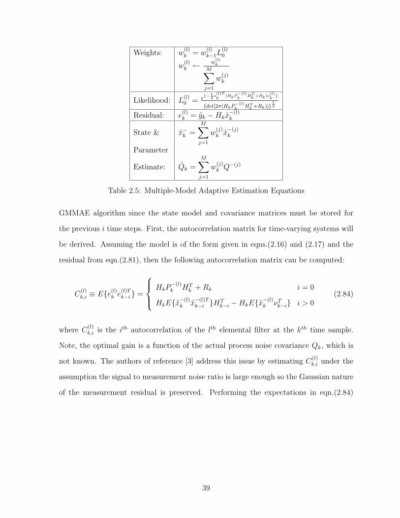
Weights: w(l)k = w
(l)k−1L
(l)0
w(l)k ←
w(l)k
M∑
j=1
w(j)k
Likelihood: L(l)0 = e
− 12 e
(l)Tk
(HkP−(l)k
HTk
+Rk)e(l)k
det[2π(HkP−(l)k
HTk
+Rk)]12
Residual: e(l)k = yk −Hkx
−(l)k
State & x−k =M
∑
j=1
w(j)k x
−(j)k
Parameter
Estimate: Qk =M
∑
j=1
w(j)k Q−(j)
Table 2.5: Multiple-Model Adaptive Estimation Equations
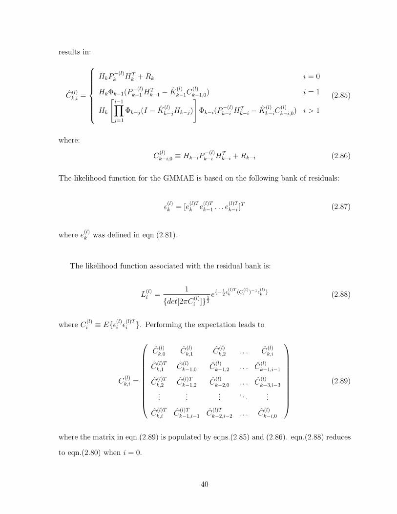
GMMAE algorithm since the state model and covariance matrices must be stored for
the previous i time steps. First, the autocorrelation matrix for time-varying systems will
be derived. Assuming the model is of the form given in eqns.(2.16) and (2.17) and the
residual from eqn.(2.81), then the following autocorrelation matrix can be computed:
C(l)k,i ≡ Ee(l)k e
(l)Tk−i =
HkP−(l)k HT
k +Rk i = 0
HkEx−(l)k x
−(l)Tk−i HT
k−i −HkEx−(l)k νT
k−i i > 0(2.84)
where C(l)k,i is the ith autocorrelation of the lth elemental filter at the kth time sample.
Note, the optimal gain is a function of the actual process noise covariance Qk, which is
not known. The authors of reference [3] address this issue by estimating C(l)k,i under the
assumption the signal to measurement noise ratio is large enough so the Gaussian nature
of the measurement residual is preserved. Performing the expectations in eqn.(2.84)
39
results in:
C(l)k,i =
HkP−(l)k HT
k +Rk i = 0
HkΦk−1(P−(l)k−1H
Tk−1 − K
(l)k−1C
(l)k−1,0) i = 1
Hk
[
i−1∏
j=1
Φk−j(I − K(l)k−jHk−j)
]
Φk−i(P−(l)k−i H
Tk−i − K
(l)k−iC
(l)k−i,0) i > 1
(2.85)
where:
C(l)k−i,0 ≡ Hk−iP
−(l)k−i H
Tk−i +Rk−i (2.86)
The likelihood function for the GMMAE is based on the following bank of residuals:
ǫ(l)k = [e
(l)Tk e
(l)Tk−1 . . . e
(l)Tk−i ]
T (2.87)
where e(l)k was defined in eqn.(2.81).
The likelihood function associated with the residual bank is:
L(l)i =
1
det[2πC(l)i ] 1
2
e−12ǫ(l)Tk
(C(l)i )−1ǫ
(l)k
(2.88)
where C(l)i ≡ Eǫ(l)i ǫ
(l)Ti . Performing the expectation leads to
C(l)k,i =
C(l)k,0 C
(l)k,1 C
(l)k,2 . . . C
(l)k,i
C(l)Tk,1 C
(l)k−1,0 C
(l)k−1,2 . . . C
(l)k−1,i−1
C(l)Tk,2 C
(l)Tk−1,2 C
(l)k−2,0 . . . C
(l)k−3,i−3
......
.... . .
...
C(l)Tk,i C
(l)Tk−1,i−1 C
(l)Tk−2,i−2 . . . C
(l)k−i,0
(2.89)
where the matrix in eqn.(2.89) is populated by eqns.(2.85) and (2.86). eqn.(2.88) reduces
to eqn.(2.80) when i = 0.
40

The overall state and unknown parameter estimates are calculated from eqns.(2.82)
and (2.83) respectively. The GMMAE equations are summarized in Table 2.6.
41

Weights: w(l)k = w
(l)k−1L
(l)i
w(l)k ←
w(l)k
M∑
j=1
w(j)k
Likelihood: L(l)i = 1
det[2πC(l)i ]
12e−
12ǫ(l)Tk
(C(l)i )−1ǫ
(l)k
when i = 0 it reduces to:
L(l)0 = 1
det[2π(HkP−(l)k
HTk
+Rk)]12e−
12e(l)Tk
(HkP−(l)k
HTk
+Rk)e(l)k
Residual: ǫ(l)k = [e
(l)Tk e
(l)Tk−1 . . . e
(l)Tk−i ]
T
where:
e(l)k = yk −Hkx
−(l)k
Autocorrelation: C(l)k,i =
C(l)k,0 C
(l)k,1 C
(l)k,2 . . . C
(l)k,i
C(l)Tk,1 C
(l)k−1,0 C
(l)k−1,2 . . . C
(l)k−1,i−1
C(l)Tk,2 C
(l)Tk−1,2 C
(l)k−2,0 . . . C
(l)k−2,i−2
......
.... . .
...
C(l)Tk,i C
(l)Tk−1,i−1 C
(l)Tk−2,i−2 . . . C
(l)k−i,0
where:
C(l)k−i,0 = Hk−i(x
−(l)k )P
−(l)k−i H
Tk−i(x
−(l)k ) +Rk−i
C(l)k,i =
Hk(x−(l)k )P
−(l)k HT
k (x−(l)k ) +Rk i = 0
Hk(x−(l)k )Φk−1(x
−(l)k )[P
−(l)k−1H
Tk−1(x
−(l)k )− Kk−1C
(l)k−1,0] i = 1
Hk(x−(l)k )
∏i−1j=1 Φk−j(x
−(l)k )[I − Kk−jHk−j(x
−(l)k )]
×Φk−i(x−(l)k )[P
−(l)k−i H
Tk−i(x
−(l)k )− Kk−iC
(l)k−i,0] i > 1
State & x−k =M
∑
j=1
w(j)k x
−(j)k
Parameter
Estimate: Qk =M
∑
j=1
w(j)k Q(j)
Table 2.6: Generalized Multiple-Model Adaptive Estimator Equations
42
Chapter 3
Analysis
This chapter presents the development of the ground truth simulator and the application
of the Generalized Multiple-Model Adaptive Estimation algorithm (GMMAE) to estimate
the unknown parameters associated with the ship tracker.
3.1 Simulation Package
This section presents the development of the ground truth simulator, including both the
kinematic and contextual data componants. Note, at certain instances the user defines
event occurances with time, whereas the simulation requires the sample number. The
conversion is accomplished with:
kevent = tevent ×K
tK(3.1)
where k denotes sample number in the range 0 ≤ k ≤ K.
3.1.1 Evolution of the Simulator
The original ground truth simulator was developed using Simulink software and utilized
the kinematic relations∫ ∫
A =∫
V = X, where X is position, V is velocity, and A is
43

acceleration. An accleration signal, A, is generated as follows:
A =
‖A‖, td ≤ t < (td + ta)
0, t < td and (td + ta) ≤ t(3.2)
where td is the ship depart time, t is the run time, and ta is the time of acceleration.
Integrating this signal results in the ship’s velocity signal. The X and Y components of
the velocity signal are:
dXdt
= VX = sinH
∫ t
0
A
dYdt
= VY = cosH
∫ t
0
A
(3.3)
where H is the heading angle calculated by eqn.(2.1), and zero initial conditions for the
integrators corresponds to a ship starting from rest. Introducing the following assump-
tions:
• Spherical Earth
• Ships do not leave the Earth’s surface: dh/dt = h = dγ/dt = γ = 0. Thus, the
Earth rotation terms can be neglected in the governing equations, i.e., the ships
will be rotating with the Earth as opposed to the Earth rotating with respect to
an airborne vehicle.
Thus, the following equations can be taken from reference [7]:
dγ
dt= tan−1
( dhdt
√
(dXdt−ReΩe cosL)2 + (dY
dt)2
)
= 0 (3.4)
dλ
dt=
dXdt
Re cosL− Ωe =
dXdt
Re cosL(3.5)
dL
dt= −
dYdt
Re
(3.6)
44
where γ is the flight path angle, h is the altitude, Re is the radius of the Earth, Ωe is the
rate of rotation of the earth, L is the latitude, and λ is the longitude.
The velocity components are used in eqns.(3.5) and (3.6) to obtain the rate of change
of longitude and latitude respectively. dλdt
and dLdt
can each be integrated to obtain the
current longitude and latitude coordinates respectively.
λ =
∫ t
0
dλ
dt
L =
∫ t
0
dL
dt
(3.7)
with initial conditions set to the departure port longitude and latitude respectively. Note,
from eqn.(3.5), the rate of change of longitude depends on the current latitude. The re-
sult is expected because the distance between longitude lines is largest at the equator
and decreases towards the poles. Thus, the current latitude must be calculated prior to
calculating dλdt
.
The current ship location coordinates are compared with the immediate destination way-
point coordinates to determine when to change bearing and head towards the next suc-
cesive waypoint. Essentially, when the ship is within a pre-defined radius of the current
destination waypoint, the next succesive waypoint is read in, and eqns.(3.5) through (3.7)
are applied to the new waypoint. The process is repeated until the destination port is
reached, at which point the velocity integrator is reset to zero, stopping the ship.
The simulator must be run at a small sample time to ensure the waypoint criterion is
not satisfied in between samples causing the simulator to fail to recognize the ship has
reached the waypoint. This is analogous to the sampling phenomenon described in Sec-
tion 2.5. In this case, the ship will maintain a constant heading for the remainder of
the simulation and spiral indefinately poleward. The requirement of using a significantly
small sampling time interval, coupled with the use of integrators, causes a simulation of
multiple ships for multiple days take hours to run and requires a large computational
45

load causing the scenarios required for the H2LIFT project to be unmanageable with
this simulator. The remainder of Section 3.1 focuses on the development of an alternate
simulator running orders of magnitude faster and with much less computational demand
than the simulator introduced here.
3.1.2 Earth Model
A spherical Earth approximation, preserving the surface area of the true Earth (RE,sphereical =
6, 371.007 km), is used for the scenario simulations since the approximation is sufficiently
accurate in the range of latitudes in which the ships will navigate. The spherical model
becomes increasingly less accurate towards the poles of the Earth, however, the latitude
range of the shipping lanes chosen for the scenarios is between 60 S and 60 N which is
far enough from the poles of the Earth to yield sufficiently accurate results. The Earth
model chosen will not effect the outcome of theH2LIFT project as long as it is consistent.
3.1.3 Velocity
The simulations apply inherent fluctuations (Vs,flux) in ship velocity about a given mean
(Vs) and contain the ability to vary Vs at a specified time. The first of these tasks is
accomplished by assigning the ship velocity as a discrete random variable of given mean
and variance. The second is accomplished by overwriting the velocity signal with a new
desired velocity over the desired set of samples. For instance, stalling a ship at sea would
be accomplished by overwriting the velocity signal with zeros over the desired stall time.
Also, the velocity signal should be overwritten with zeros for times less than the ship
departure time and those greater than its arrival time to represent the ship being docked
at port.
46
3.1.4 Sample Times: Constant vs. Varying
Depending on the use of the simulator, the user might prefer to choose between a constant
and a varying sample time. For example, if the simulator is used to tune the estimation
filter in the ship tracking algorithm, a constant sample time is required. However, if
the simulator output is to emulate sensor data from an Unmanned Air Vehicle (UAV), a
varying sample time would be more appropriate. The simulator is set up so the user has
the option to choose between the two.
A constant sample time is implemented by defining a simulation run time (tK) and the
total number of desired samples (K). The sample time is then calculated for each ship
as Ts = tKK
. A varying sample time is implemented by generating K random numbers on
the range of 0 ≤ tk ≤ tK and sorting in ascending order. The mean and variance of the
random numbers should be chosen such that the desired sample density and distribution
is achieved.
3.1.5 Navigation/Methodology
Each shipping route in its entirety will be made up of a series of short rhumb line seg-
ments between consecutive waypoints in order to avoid land masses. Since each individual
rhumb line segment will be relatively short, the difference in route length as compared to
using great circle navigation will be minimal while the advantage of programming simplic-
ity will be substantial. The navigation methodology is described here, and summarized
in the flowchart shown in Figure 3.1.
1. Prior to entering the main loop of the program, the following vectors are calculated:
• Heading angles between each successive waypoint in the route using eqn. (2.1).
• Running distance from the departure port to each waypoint,n, by summing the
distances between each succesive waypoint less than n, for for every waypoint
47
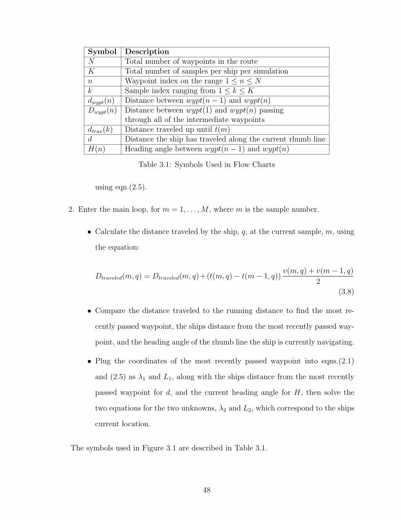
Symbol DescriptionN Total number of waypoints in the routeK Total number of samples per ship per simulationn Waypoint index on the range 1 ≤ n ≤ Nk Sample index ranging from 1 ≤ k ≤ Kdwypt(n) Distance between wypt(n− 1) and wypt(n)Dwypt(n) Distance between wypt(1) and wypt(n) passing
through all of the intermediate waypointsdtrav(k) Distance traveled up until t(m)d Distance the ship has traveled along the current rhumb lineH(n) Heading angle between wypt(n− 1) and wypt(n)
Table 3.1: Symbols Used in Flow Charts
using eqn.(2.5).
2. Enter the main loop, for m = 1, . . . ,M , where m is the sample number.
• Calculate the distance traveled by the ship, q, at the current sample, m, using
the equation:
Dtraveled(m, q) = Dtraveled(m, q)+(t(m, q)− t(m− 1, q))v(m, q) + v(m− 1, q)
2
(3.8)
• Compare the distance traveled to the running distance to find the most re-
cently passed waypoint, the ships distance from the most recently passed way-
point, and the heading angle of the rhumb line the ship is currently navigating.
• Plug the coordinates of the most recently passed waypoint into eqns.(2.1)
and (2.5) as λ1 and L1, along with the ships distance from the most recently
passed waypoint for d, and the current heading angle for H, then solve the
two equations for the two unknowns, λ2 and L2, which correspond to the ships
current location.
The symbols used in Figure 3.1 are described in Table 3.1.
48

Figure 3.1: Navigation Methodology
3.1.6 Crossing the Prime Meridian
Eqns.(2.1) and (2.5) are not valid for routes passing over the prime meridian. Specifically,
a jump discontinuity from 180 to −180 longitude exists, thus, the derived ship positions
using eqns.(2.1) and (2.5) proceed in the opposite direction around the Earth (through 0
longitude) when encountering this discontinuity. However, the input to these equations
can be conditioned to obtain the intended results. First, consider the case where a route
crosses the prime meridian from the Western to Eastern hemispheres. The following
steps can be used to correct for this inadequacy, as shown in the flow charts in Figures
3.2 and 3.3:
1. Subtract 360 from all eastern waypoints.
2. Perform calculations.
3. Add 360 to all points along the resulting ship track less than −180.
49

Likewise, if the route crosses from East to West then:
1. Add 360 to all western waypoints.
2. Perform calculations.
3. Subtract 360 to all points along the resulting ship track greater than 180.
3.1.7 Ship Stall and Rescue Helicopters
The simulator has the ability to stall a ship at sea. Once stalled, a rescue helicopter flies
out to the ship and repairs it, at which point the helicopter will return to base and the
ship will resume its course. The feature is commanded by the user defining a stall ship
(qstall), time of stall (tstall), rescue delay time (δrescue), and repair time (δrepair), as well
as some helicopter paramters including, altitude (h), mean velocity (Vh), and magnitude
of velocity variations about the mean (Vh,flux). Rescue delay time, δrescue, refers to the
amount of time delay between the ship stalling and the helicopter departing, δrescue =
th,d−tstall, where th,d is the helicopter departure time. The ship is stalled by overwriting its
velocity signal with zeros for kstall ≤ k < kresume, with, kevent = tevent× KtK
. Note, kresume
is unknown at the start of the simulation and depends on the helicopter parameters.
A rescue helicopter is implemented by creating a function to be called from the main
routine of the simulation code. This function should contain the velocity generation and
navigation algorithms introduced in Sections 3.1.3 and 3.1.5, appropriately tailored for
the helicopter. The specific changes are as follows:
• Re is replaced with Re +h in eqn.(2.5) to account for the altitude of the helicopter.
• th,d = tstall + δrescue.
• The helicopter route has 2 waypoints (N = 2 in the flowchart in Figure 3.1); the
departure base coordinates and the destination coordinates, i.e. the stall location
of the ship (L(kstall), λ(kstall)).
50

Figure 3.2: Longitude Conditioning
51
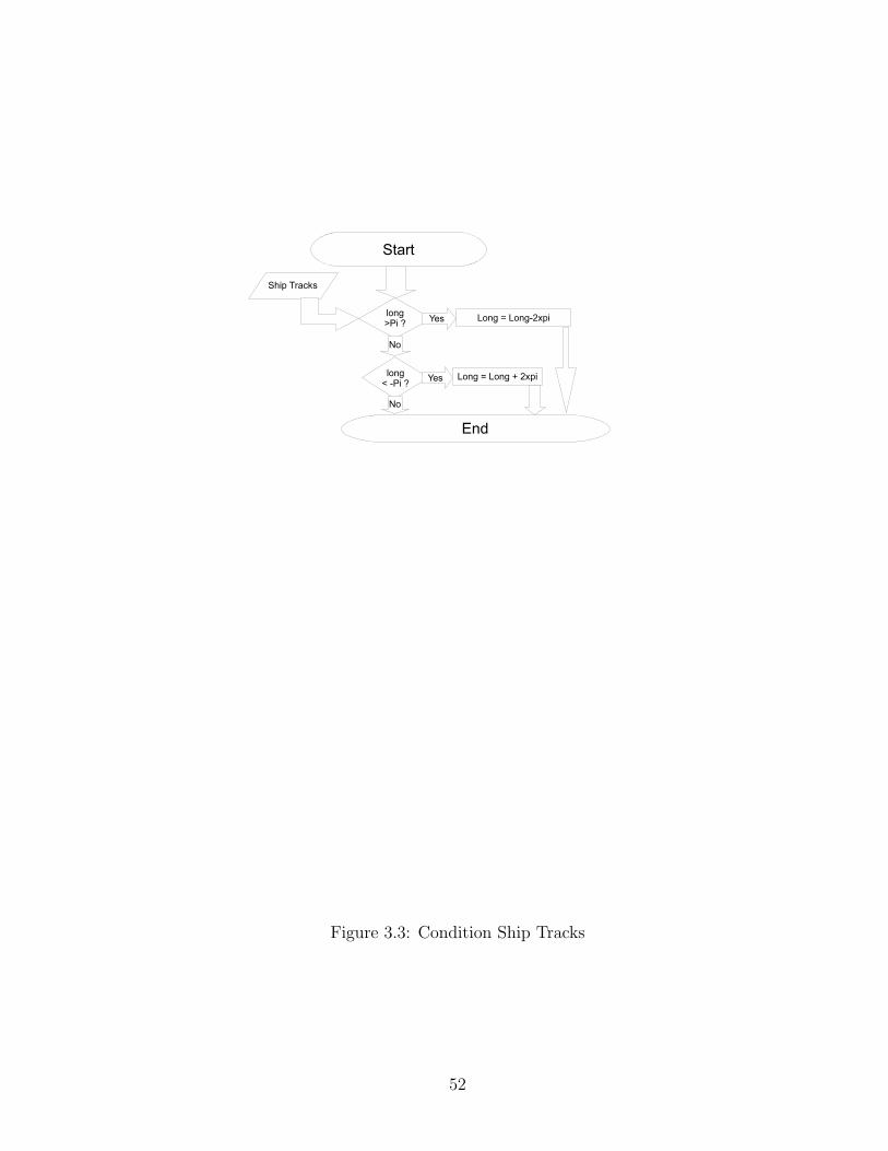
Figure 3.3: Condition Ship Tracks
52
• The helicopter function can be simplified to only handle one helicopter as it will
be called individually for each stalled ship. This is because tresume depends on the
helicopter parameters, and the helicopter destination waypoints depend on the ship
parameters, thus the helicopter function must be called at a unique time for each
ship.
The flowchart in Figure 3.1 is propagated in a loop for q = 1 . . . Q to implement multiple
ships, where q is the ship index and Q is the total number of ships. Because of the mu-
tual dependence of the rescue helicopter and the stalled ship, it is vital for the helicopter
function to be called when q = qstall and k = kstall, for each ship, where qstall is the stall
ship and kstall is the stall sample. At this point, the stall location is known and can be
sent to the helicopter function which will return kresume. kresume is used to overwrite the
ships velocity signal with zeros for kstall ≤ t < kresume, hence stalling the ship.
Note, the helicopter must return to the base it departed from. This is accomplished
by mirroring its velocity, latitude, and longitude signals about the point kh,arrive +
ceil
δrepairK
2tK
and cropping it at k = K, where kh,arrive denotes the sample in which
the helicopter arrives on the ship.
When choosing ship stall times it is important to ensure the stall times occur while
the ship is in route to avoid errors in the helicopter function, i.e. kdepart < kstall <
karrive. Since tdepart, tstall, tK , and K are inputs to the simulator, the user can ensure
kdepart < kstall before runing the simulation, however karrive is unknown at the start of
the simulation, thus it must be approximated with the following equation:
karrive =Dwypt(N)
max(V )× K
tK(3.9)
where Dwypt(N) denotes the total route distance, max(V ) denotes the maximum ship
velocity, K denotes the number of samples per ship per simulation, and tK denotes the
53
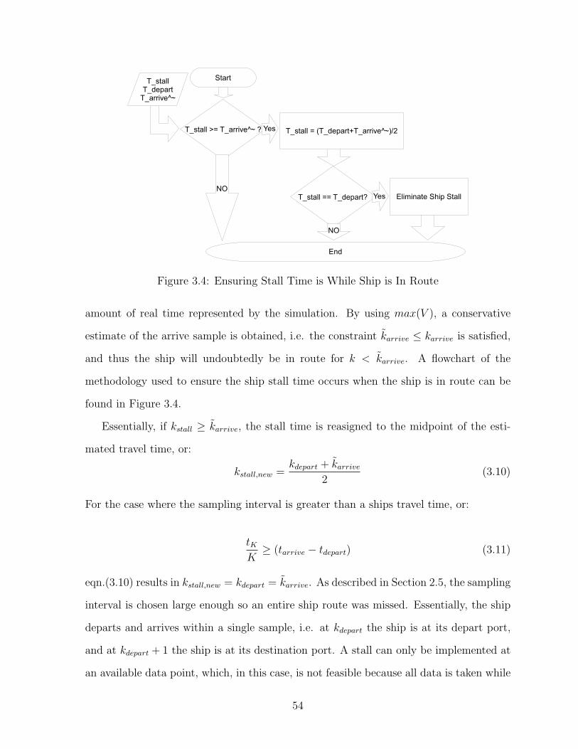
Figure 3.4: Ensuring Stall Time is While Ship is In Route
amount of real time represented by the simulation. By using max(V ), a conservative
estimate of the arrive sample is obtained, i.e. the constraint karrive ≤ karrive is satisfied,
and thus the ship will undoubtedly be in route for k < karrive. A flowchart of the
methodology used to ensure the ship stall time occurs when the ship is in route can be
found in Figure 3.4.
Essentially, if kstall ≥ karrive, the stall time is reasigned to the midpoint of the esti-
mated travel time, or:
kstall,new =kdepart + karrive
2(3.10)
For the case where the sampling interval is greater than a ships travel time, or:
tKK≥ (tarrive − tdepart) (3.11)
eqn.(3.10) results in kstall,new = kdepart = karrive. As described in Section 2.5, the sampling
interval is chosen large enough so an entire ship route was missed. Essentially, the ship
departs and arrives within a single sample, i.e. at kdepart the ship is at its depart port,
and at kdepart + 1 the ship is at its destination port. A stall can only be implemented at
an available data point, which, in this case, is not feasible because all data is taken while
54

the ship is docked. Therefore, the simulator assumes the ship also stalls and is repaired
within the same sample interval as departing and arriving, and proceeds computations
as if a stall does not occur as shown in Figure 3.4. This is analogous to an event occuring
between sensor measurements and thus not being detected. All discrete systems are at
risk of this sampling phenomenon described in Section 2.5.
3.1.8 Contextual Information
The contextual information portion of the maritime scenarios is added using code written
in Matlab. The inputs to the contextual assignment code are Ship Number, and Foreign
Probability, where Ship Number, Sq, refers to the number assigned to the desired ship
from the ship information database, and Foreign Probability, Pq, refers to the probabil-
ity that each crew member is of a nationality different from the flag the ship is flying.
Note, subscript q denotes the scenario ship number (different from the ship information
database ship number) and is on the range 1 ≤ q ≤ Q. Therefore, Sq assigns ship number
S’s information from the ship information database to the qth ship in the scenario.
The ship information database contains the available information for all of the ships in-
cluding: ship name, ship owner, year built, length, beam, maximum TEU, gross weight,
maximum speed, flag flown, and number of crew members(Lq). The crew member infor-
mation database includes the crew member information for all the available crew members
including: name, nationality, date of birth, and position held.
The user inputs the desired Sq’s for ships in the scenario (ships 1. . .Q), or has them
randomly selected, and the contextual assignment code reads in all of the corresponding
ship information from the ship information database and randomly selects crew mem-
bers for each ship based on a probability model. The number of crew members selected
for each ship will correspond to the amount specified for the particular ship in the ship
information database. The probability model selects the crew members based on their
respective nationality and Pq. It does so by generating random numbers, βq,l, between 0
55
and 1, where subscript l is an index for the crew members and is on the range 1 ≤ l ≤ Lq.
Therefore, if βq,l ≤ Pq, the lth crew member on ship q will have a different nationality
than displayed on ship q’s flag. Conversely, if βq,l > Pq, then the nationality of the lth
crew member on ship q will match ship q’s displayed flag.
The contextual information is stored in structure format. For example, to output the
date of birth of the captain on the qth scenario ship one would type:
>Shipq.CrewMembers.Captain.DOB
The contextual information structure format is in Table 3.2.
3.2 Parameter Estimation for Tuning
A Generalized Multiple-Model Adaptive estimation algorithm (introduced in Section 2.9)
is used to tune a state estimator made up of a Probabilistic Data Association Filter
(introduced in Section 2.7) and Kalman filters (introduced in Section 2.6). The state
estimator is used to track the ships involved in the H2LIFT scenarios, generated by
the ground truth simulator introduced in Section 3.1. Prior to this work, the state
estimator was tuned by hand in an ad-hoc process. The system model for the ship
tracking application is as follows:
xk =
x
δxδt
y
δy
δt
,Φ =
1 Ts 0 0
0 1 0 0
0 0 1 Ts
0 0 0 1
, uk = 0
Where Ts is the sampling interval, tk − tk−1. Therefore eqn.(2.16) becomes:
56
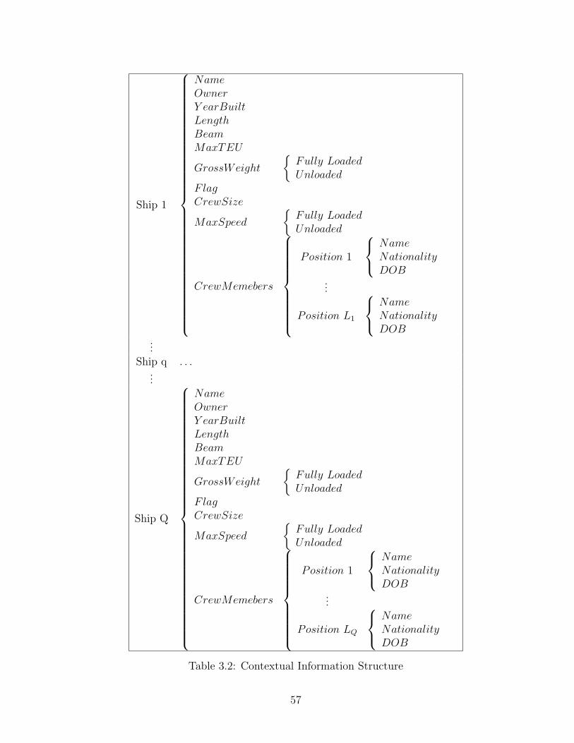
Ship 1
NameOwnerY earBuiltLengthBeamMaxTEU
GrossWeight
Fully LoadedUnloaded
F lagCrewSize
MaxSpeed
Fully LoadedUnloaded
CrewMemebers
Position 1
NameNationalityDOB
...
Position L1
NameNationalityDOB
...Ship q . . .
...
Ship Q
NameOwnerY earBuiltLengthBeamMaxTEU
GrossWeight
Fully LoadedUnloaded
F lagCrewSize
MaxSpeed
Fully LoadedUnloaded
CrewMemebers
Position 1
NameNationalityDOB
...
Position LQ
NameNationalityDOB
Table 3.2: Contextual Information Structure
57

x
δxδt
y
δy
δt
k+1
=
1 Ts 0 0
0 1 0 0
0 0 1 Ts
0 0 0 1
x
δxδt
y
δy
δt
k
+ Υwk (3.12)
where wk is a zero-mean Gaussian process with covariance described by:
Q =
qy
T 3s
3T 2
s
2
T 2s
2Ts
0 0
0 0
0 0
0 0qx
T 3s
3T 2
s
2
T 2s
2Ts
(3.13)
In order to properly tune the filter, estimates of the system process noise parameters, qx
and qy used in the Kalman filter equations as well as probability parameters PD and PG
from eqn.(2.63) must be obtained. The GMMAE algorithm was used to estimate these
parameters and tune the PDAF.
58

Chapter 4
Simulation, Demonstration, and
Discussion
This chapter presents simulation results from both the simulation package presented in
Section 3.1 and the adaptive ship tracker presented in Section 3.2. Four scenarios are
generated in Section 4.1 to demonstrate the capabilities of the simulation package and
one ship is tracked to demonstrate the performance of the ship tracker when tuned using
the GMMAE algorithm.
4.1 Ground Truth Simulator
4.1.1 Scenario 1
The first scenario involves 3 ships with simulation inputs described in Table 4.1. Ship 1
departs from Oakland, CA, USA and is destined for Shanghai, China (ports emphasized
with squares), ship 2 departs from Bremerhaven, Germany and is destined for Charleston,
SC, USA (ports emphasized with circles), and ship 3 departs from Beirut, Lebanon and is
destined for New York, NY, USA (ports emphasized with triangles). Figure 4.1 displays
the resulting ship tracks for a constant sample time, Figure 4.2 displays the resulting ship
59
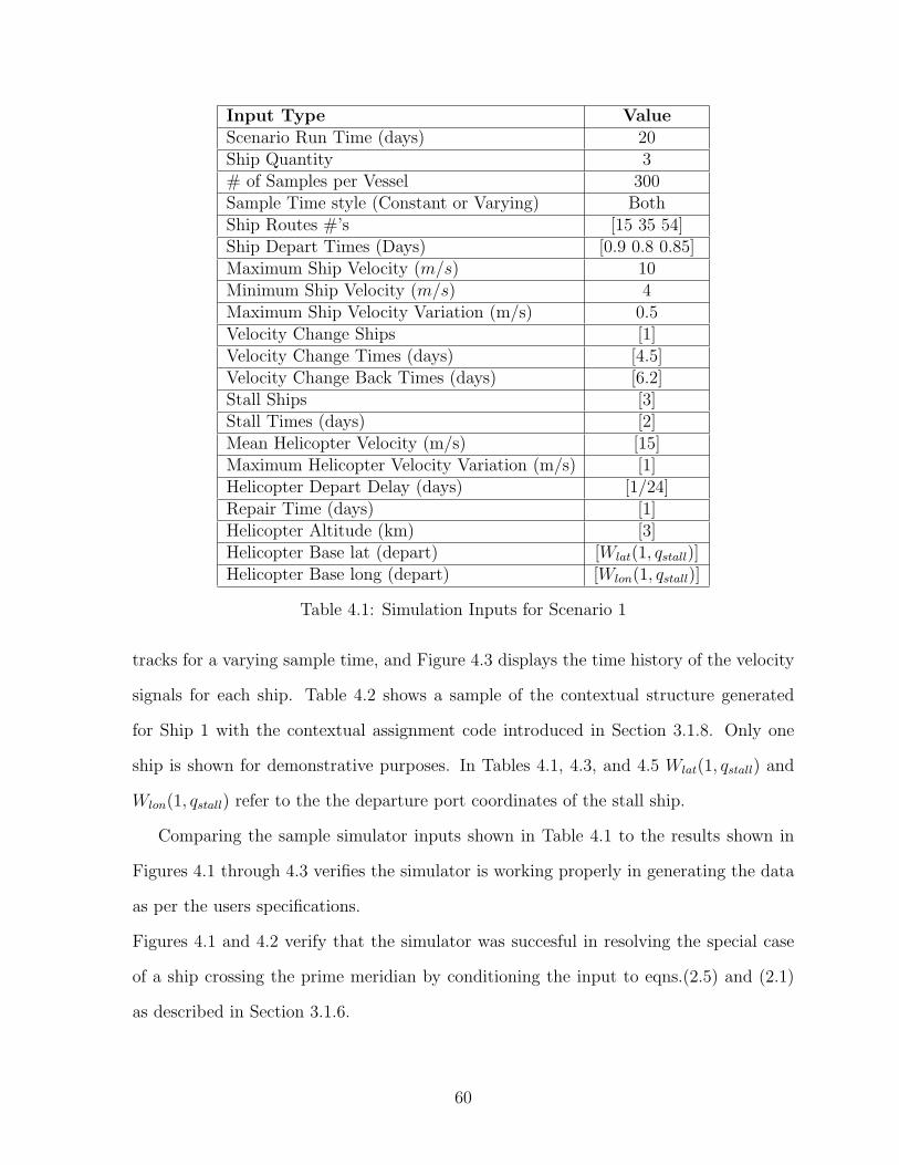
Input Type ValueScenario Run Time (days) 20Ship Quantity 3# of Samples per Vessel 300Sample Time style (Constant or Varying) BothShip Routes #’s [15 35 54]Ship Depart Times (Days) [0.9 0.8 0.85]Maximum Ship Velocity (m/s) 10Minimum Ship Velocity (m/s) 4Maximum Ship Velocity Variation (m/s) 0.5Velocity Change Ships [1]Velocity Change Times (days) [4.5]Velocity Change Back Times (days) [6.2]Stall Ships [3]Stall Times (days) [2]Mean Helicopter Velocity (m/s) [15]Maximum Helicopter Velocity Variation (m/s) [1]Helicopter Depart Delay (days) [1/24]Repair Time (days) [1]Helicopter Altitude (km) [3]Helicopter Base lat (depart) [Wlat(1, qstall)]Helicopter Base long (depart) [Wlon(1, qstall)]
Table 4.1: Simulation Inputs for Scenario 1
tracks for a varying sample time, and Figure 4.3 displays the time history of the velocity
signals for each ship. Table 4.2 shows a sample of the contextual structure generated
for Ship 1 with the contextual assignment code introduced in Section 3.1.8. Only one
ship is shown for demonstrative purposes. In Tables 4.1, 4.3, and 4.5 Wlat(1, qstall) and
Wlon(1, qstall) refer to the the departure port coordinates of the stall ship.
Comparing the sample simulator inputs shown in Table 4.1 to the results shown in
Figures 4.1 through 4.3 verifies the simulator is working properly in generating the data
as per the users specifications.
Figures 4.1 and 4.2 verify that the simulator was succesful in resolving the special case
of a ship crossing the prime meridian by conditioning the input to eqns.(2.5) and (2.1)
as described in Section 3.1.6.
60
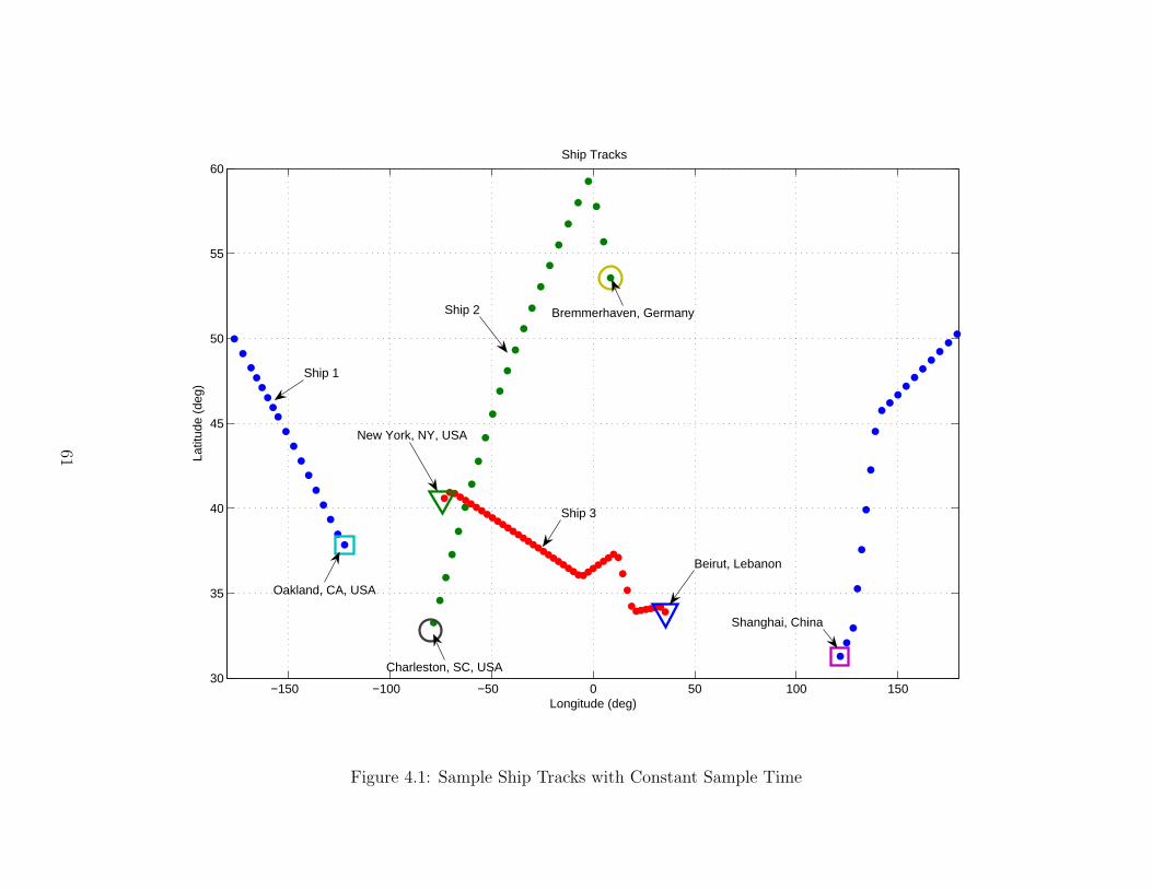
−150 −100 −50 0 50 100 15030
35
40
45
50
55
60Ship Tracks
Longitude (deg)
Latit
ude
(deg
)
Bremmerhaven, Germany
Charleston, SC, USA
Oakland, CA, USA
New York, NY, USA
Beirut, Lebanon
Shanghai, China
Ship 1
Ship 2
Ship 3
Figure 4.1: Sample Ship Tracks with Constant Sample Time
61

−150 −100 −50 0 50 100 15030
35
40
45
50
55
60Ship Tracks
Longitude (deg)
Latit
ude
(deg
)
Oakland, CA, USA
Bremerhaven, Germany
New York, NY, USA
Charleston, SC, USA
Beirut, Lebanon
Shanghai, China
Ship 1
Ship 2
Ship 3
Figure 4.2: Sample Ship Tracks with Varying Sample Time
62
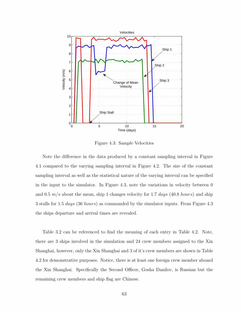
0 5 10 15 200
1
2
3
4
5
6
7
8
9
10Velocities
Time (days)
Vel
ocity
(m
/s)
Ship Stall
Change of MeanVelocity
Ship 1
Ship 2
Ship 3
Figure 4.3: Sample Velocities
Note the difference in the data produced by a constant sampling interval in Figure
4.1 compared to the varying sampling interval in Figure 4.2. The size of the constant
sampling interval as well as the statistical nature of the varying interval can be specified
in the input to the simulator. In Figure 4.3, note the variations in velocity between 0
and 0.5 m/s about the mean, ship 1 changes velocity for 1.7 days (40.8 hours) and ship
3 stalls for 1.5 days (36 hours) as commanded by the simulator inputs. From Figure 4.3
the ships departure and arrival times are revealed.
Table 3.2 can be referenced to find the meaning of each entry in Table 4.2. Note,
there are 3 ships involved in the simulation and 24 crew members assigned to the Xin
Shanghai, however, only the Xin Shanghai and 3 of it’s crew members are shown in Table
4.2 for demonstrative purposes. Notice, there is at least one foreign crew member aboard
the Xin Shanghai. Specifically the Second Officer, Gosha Danilov, is Russian but the
remaining crew members and ship flag are Chinese.
63

Ship 1
Xin ShanghaiChina Shipping Container Lines2006336.7m45.6m9, 580
Gross Weight
108, 500107, 200
China24
Max Speed
6.5ms
8ms
CrewMemebers
Captain
Dao He WuChinese8/26/61
Chief Officer
Dao Ma KungChinese3/7/85
Second Officer
Gosha DanilovRussian12/30/56
...
Machinist
Ti KungzhengChinese7/16/77
Table 4.2: Contextual Information Structure
64
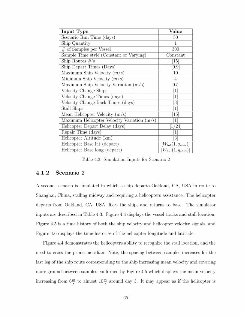
Input Type ValueScenario Run Time (days) 30Ship Quantity 1# of Samples per Vessel 300Sample Time style (Constant or Varying) ConstantShip Routes #’s [15]Ship Depart Times (Days) [0.9]Maximum Ship Velocity (m/s) 10Minimum Ship Velocity (m/s) 4Maximum Ship Velocity Variation (m/s) 0.5Velocity Change Ships [1]Velocity Change Times (days) [1]Velocity Change Back Times (days) [3]Stall Ships [1]Mean Helicopter Velocity (m/s) [15]Maximum Helicopter Velocity Variation (m/s) [1]Helicopter Depart Delay (days) [1/24]Repair Time (days) [1]Helicopter Altitude (km) [3]Helicopter Base lat (depart) [Wlat(1, qstall)]Helicopter Base long (depart) [Wlon(1, qstall)]
Table 4.3: Simulation Inputs for Scenario 2
4.1.2 Scenario 2
A second scenario is simulated in which a ship departs Oakland, CA, USA in route to
Shanghai, China, stalling midway and requiring a helicopters assistance. The helicopter
departs from Oakland, CA, USA, fixes the ship, and returns to base. The simulator
inputs are described in Table 4.3. Figure 4.4 displays the vessel tracks and stall location,
Figure 4.5 is a time history of both the ship velocity and helicopter velocity signals, and
Figure 4.6 displays the time histories of the helicopter longitude and latitude.
Figure 4.4 demonstrates the helicopters ability to recognize the stall location, and the
need to cross the prime meridian. Note, the spacing between samples increases for the
last leg of the ship route corresponding to the ship increasing mean velocity and covering
more ground between samples confirmed by Figure 4.5 which displays the mean velocity
increasing from 6ms
to almost 10ms
around day 3. It may appear as if the helicopter is
65

−150 −100 −50 0 50 100 15030
35
40
45
50
55
Longitude (degrees)
Latit
ude
(deg
rees
)
Helicopter Rescue
Ship
Helicopter
Oakland, CA, USA
Shanghai, China
Stall Site
Figure 4.4: Rescue Helicopter
66
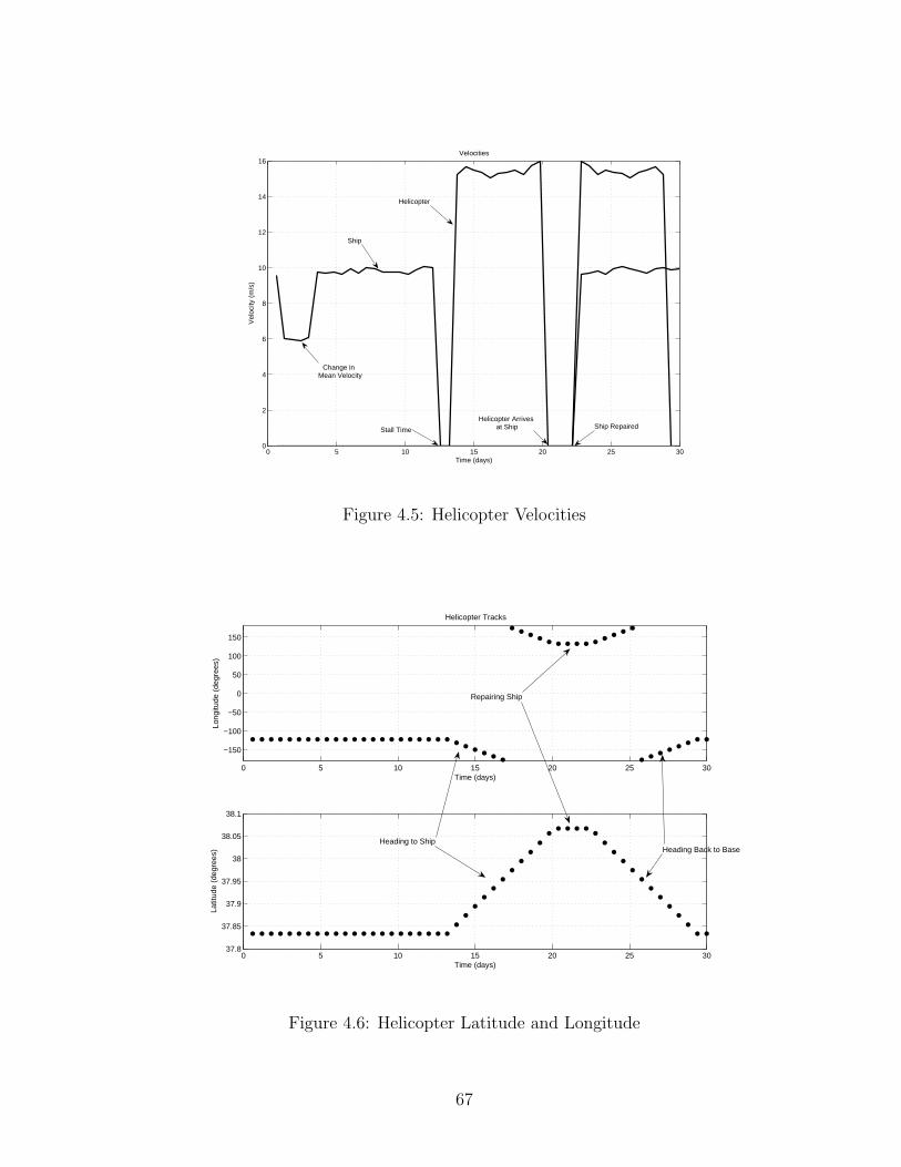
0 5 10 15 20 25 300
2
4
6
8
10
12
14
16
Time (days)
Vel
ocity
(m
/s)
Velocities
Ship
Stall Time
Helicopter Arrives at Ship
Helicopter
Ship Repaired
Change in Mean Velocity
Figure 4.5: Helicopter Velocities
0 5 10 15 20 25 30
−150
−100
−50
0
50
100
150
Time (days)
Long
itude
(de
gree
s)
Helicopter Tracks
0 5 10 15 20 25 3037.8
37.85
37.9
37.95
38
38.05
38.1
Time (days)
Latit
ude
(deg
rees
)
Heading to Ship
Repairing Ship
Heading Back to Base
Figure 4.6: Helicopter Latitude and Longitude
67
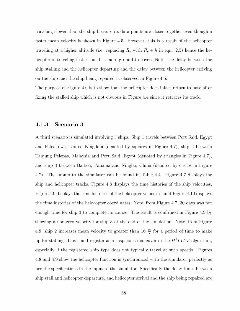
traveling slower than the ship because its data points are closer together even though a
faster mean velocity is shown in Figure 4.5. However, this is a result of the helicopter
traveling at a higher altitude (i.e. replacing Re with Re + h in eqn. 2.5) hence the he-
licopter is traveling faster, but has more ground to cover. Note, the delay between the
ship stalling and the helicopter departing and the delay between the helicopter arriving
on the ship and the ship being repaired ia observed in Figure 4.5.
The purpose of Figure 4.6 is to show that the helicopter does infact return to base after
fixing the stalled ship which is not obvious in Figure 4.4 since it retraces its track.
4.1.3 Scenario 3
A third scenario is simulated involving 3 ships. Ship 1 travels between Port Said, Egypt
and Felixstowe, United Kingdom (denoted by squares in Figure 4.7), ship 2 between
Tanjung Pelepas, Malaysia and Port Said, Egypt (denoted by triangles in Figure 4.7),
and ship 3 between Balboa, Panama and Ningbo, China (denoted by circles in Figure
4.7). The inputs to the simulator can be found in Table 4.4. Figure 4.7 displays the
ship and helicopter tracks, Figure 4.8 displays the time histories of the ship velocities,
Figure 4.9 displays the time histories of the helicopter velocities, and Figure 4.10 displays
the time histories of the helocopter coordinates. Note, from Figure 4.7, 30 days was not
enough time for ship 3 to complete its course. The result is confirmed in Figure 4.9 by
showing a non-zero velocity for ship 3 at the end of the simulation. Note, from Figure
4.9, ship 2 increases mean velocity to greater than 16 ms
for a period of time to make
up for stalling. This could register as a suspicious maneuver in the H2LIFT algorithm,
especially if the registered ship type does not typically travel at such speeds. Figures
4.8 and 4.9 show the helicopter function is synchronized with the simulator perfectly as
per the specifications in the input to the simulator. Specifically the delay times between
ship stall and helicopter departure, and helicopter arrival and the ship being repaired are
68
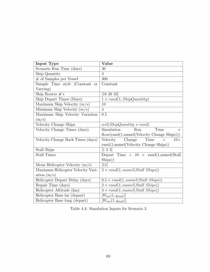
Input Type ValueScenario Run Time (days) 30Ship Quantity 3# of Samples per Vessel 300Sample Time style (Constant orVarying)
Constant
Ship Routes #’s [16 26 33]Ship Depart Times (Days) 1× rand(1, ShipQuantity)Maximum Ship Velocity (m/s) 10Minimum Ship Velocity (m/s) 4Maximum Ship Velocity Variation(m/s)
0.5
Velocity Change Ships ceil(ShipQuantity × rand)Velocity Change Times (days) Simulation Run Time ×
floor(rand(1,numel(Velocity Change Ships)))Velocity Change Back Times (days) Velocity Change Time + 10×
rand(1,numel(Velocity Change Ships))Stall Ships [1 2 3]Stall Times Depart Time + 10 × rand(1,numel(Stall
Ships))Mean Helicopter Velocity (m/s) [15]Maximum Helicopter Velocity Vari-ation (m/s)
2× rand(1, numel(Stall Ships))
Helicopter Depart Delay (days) 0.5× rand(1, numel(Stall Ships))Repair Time (days) 2× rand(1, numel(Stall Ships))Helicopter Altitude (km) 3× rand(1, numel(Stall Ships))Helicopter Base lat (depart) [Wlat(1, qstall)]Helicopter Base long (depart) [Wlon(1, qstall)]
Table 4.4: Simulation Inputs for Scenario 3
69
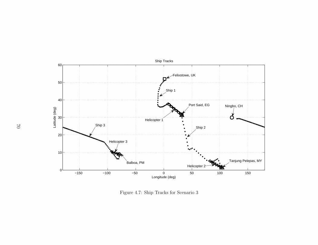
−150 −100 −50 0 50 100 1500
10
20
30
40
50
60
Longitude (deg)
Latit
ude
(deg
)
Ship Tracks
Balboa, PM
Ship 3
Helicopter 3
Felixstowe, UK
Ship 1
Helicopter 1
Port Said, EG
Ship 2
Helicopter 2
Tanjung Pelepas, MY
Ningbo, CH
Figure 4.7: Ship Tracks for Scenario 3
70
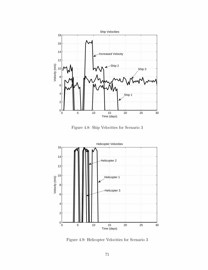
0 5 10 15 20 25 300
2
4
6
8
10
12
14
16
18Ship Velocities
Time (days)
Vel
ocity
(m
/s)
Ship 1
Ship 2Ship 3
Increased Velocity
Figure 4.8: Ship Velocities for Scenario 3
0 5 10 15 20 25 300
2
4
6
8
10
12
14
16Helicopter Velocities
Time (days)
Vel
ocity
(m
/s) Helicopter 1
Helicopter 2
Helicopter 3
Figure 4.9: Helicopter Velocities for Scenario 3
71
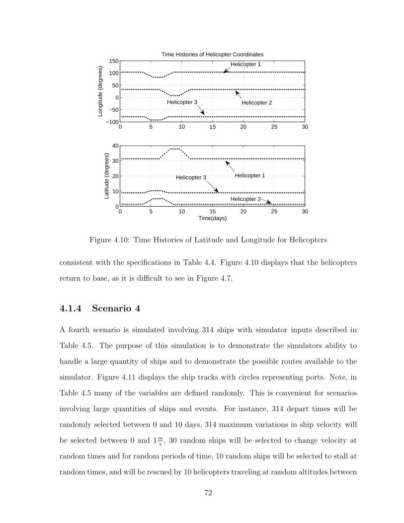
0 5 10 15 20 25 30−100
−50
0
50
100
150
Long
itude
(de
gree
s)
Time Histories of Helicopter Coordinates
0 5 10 15 20 25 300
10
20
30
40
Time(days)
Latit
ude
(deg
rees
)
Helicopter 1
Helicopter 2Helicopter 3
Helicopter 1
Helicopter 2
Helicopter 3
Figure 4.10: Time Histories of Latitude and Longitude for Helicopters
consistent with the specifications in Table 4.4. Figure 4.10 displays that the helicopters
return to base, as it is difficult to see in Figure 4.7.
4.1.4 Scenario 4
A fourth scenario is simulated involving 314 ships with simulator inputs described in
Table 4.5. The purpose of this simulation is to demonstrate the simulators ability to
handle a large quantity of ships and to demonstrate the possible routes available to the
simulator. Figure 4.11 displays the ship tracks with circles representing ports. Note, in
Table 4.5 many of the variables are defined randomly. This is convenient for scenarios
involving large quantities of ships and events. For instance, 314 depart times will be
randomly selected between 0 and 10 days, 314 maximum variations in ship velocity will
be selected between 0 and 1ms
, 30 random ships will be selected to change velocity at
random times and for random periods of time, 10 random ships will be selected to stall at
random times, and will be rescued by 10 helicopters traveling at random altitudes between
72
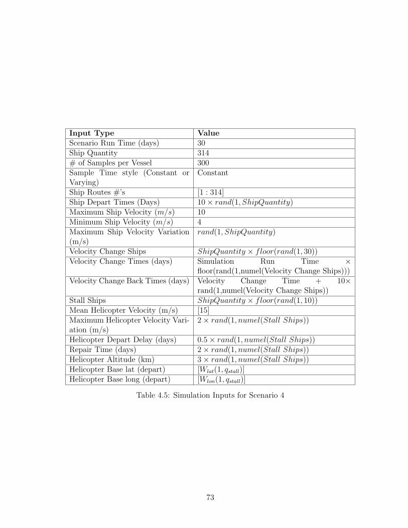
Input Type ValueScenario Run Time (days) 30Ship Quantity 314# of Samples per Vessel 300Sample Time style (Constant orVarying)
Constant
Ship Routes #’s [1 : 314]Ship Depart Times (Days) 10× rand(1, ShipQuantity)Maximum Ship Velocity (m/s) 10Minimum Ship Velocity (m/s) 4Maximum Ship Velocity Variation(m/s)
rand(1, ShipQuantity)
Velocity Change Ships ShipQuantity × floor(rand(1, 30))Velocity Change Times (days) Simulation Run Time ×
floor(rand(1,numel(Velocity Change Ships)))Velocity Change Back Times (days) Velocity Change Time + 10×
rand(1,numel(Velocity Change Ships))Stall Ships ShipQuantity × floor(rand(1, 10))Mean Helicopter Velocity (m/s) [15]Maximum Helicopter Velocity Vari-ation (m/s)
2× rand(1, numel(Stall Ships))
Helicopter Depart Delay (days) 0.5× rand(1, numel(Stall Ships))Repair Time (days) 2× rand(1, numel(Stall Ships))Helicopter Altitude (km) 3× rand(1, numel(Stall Ships))Helicopter Base lat (depart) [Wlat(1, qstall)]Helicopter Base long (depart) [Wlon(1, qstall)]
Table 4.5: Simulation Inputs for Scenario 4
73

0 and 3 km, departing from their corresponding stalled ship departure port with random
depart delays between 0 and 12 hours, and random repair times are selected between 0
and 2 days. Note, the tracks that appear to be traveling over land are either helicopters
or ships traveling through rivers. The tracks that do not terminate at a destination port
(denoted with a circle) are those that were still in route when the simulation ended.
The simulator runs fairly quickly, generating data for the 314 ships in a few seconds.
Many more ships could be simulated without a problem, but for presentations sake only
314 were chosen to keep Figure 4.11 relatively uncluttered. The single limitation on the
amount of data produced (a funciton of ship quantity and number of samples per ship)
is the amount of memory available on the computer being used to run the simulator.
4.2 Parameter Estimation
4.2.1 First Simulation
In the first simulation, the ship track estimator is propogated using a GMMAE algorithm
with 5 residuals in the residual bank and 40 parallel Kalman filters are used to estimate
the unknown paramters PD (probability the correct measurement will not be detected by
the PDAF), PG (probability the correct measurement will not lie in the validation region
used by the PDAF), qlat, and qlong (process noise parameters used by the Kalman filters)
needed to properly tune the ship track estimator. Figure 4.12 displays a time history
demonstrating how the weights vary as the GMMAE algorithm converges. Figures 4.13,
4.14, 4.15, and 4.16 display time histories of the unknown parameter convergence. Note,
in Figure 4.12 one filter emerges as being dominant, however, a few other filters continue
to contribute minimally throughout the tracking process.
Figure 4.17 through 4.20 show the performance of the state estimator using the con-
verged values of PD,PG, qlat, and qlong. Figure 4.17 displays the time history of the error
74
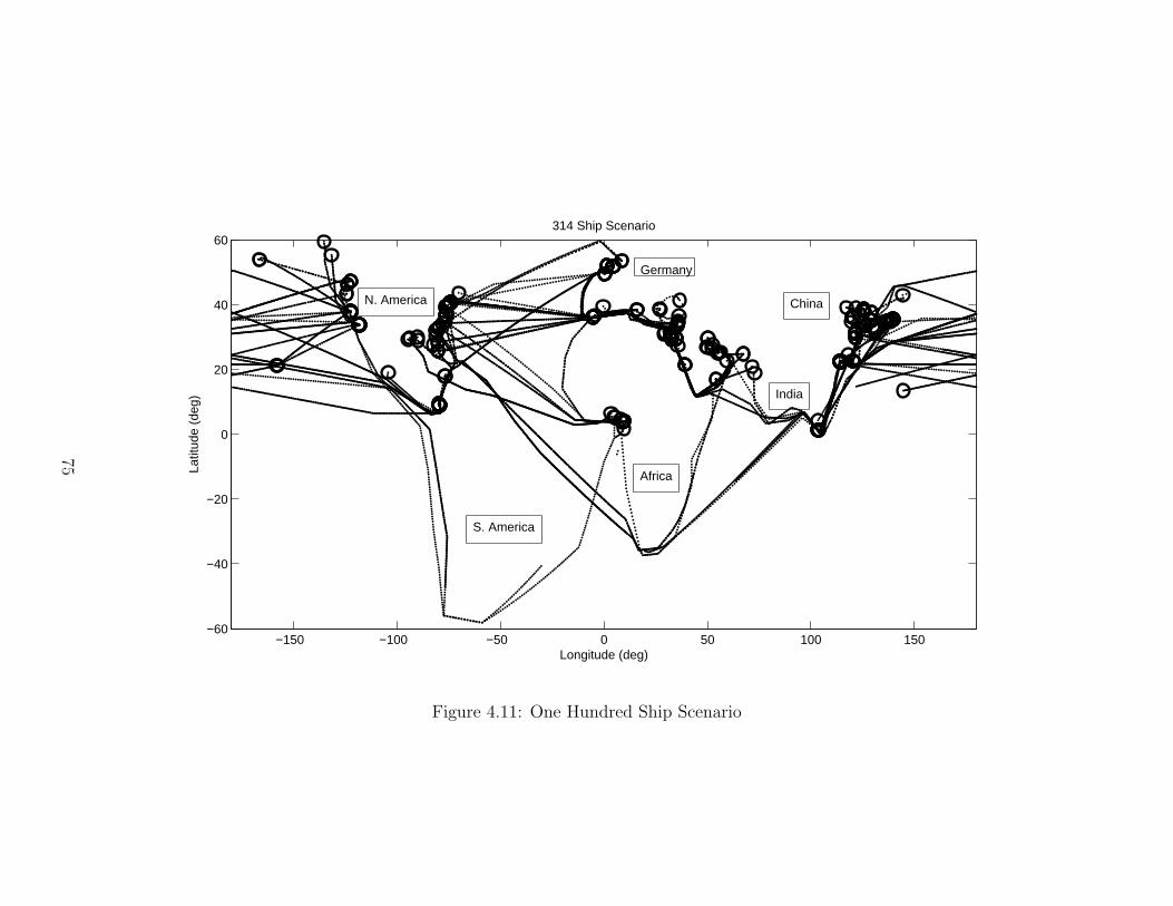
−150 −100 −50 0 50 100 150−60
−40
−20
0
20
40
60314 Ship Scenario
Longitude (deg)
Latit
ude
(deg
)
N. America
S. America
Africa
India
China
Germany
Figure 4.11: One Hundred Ship Scenario
75
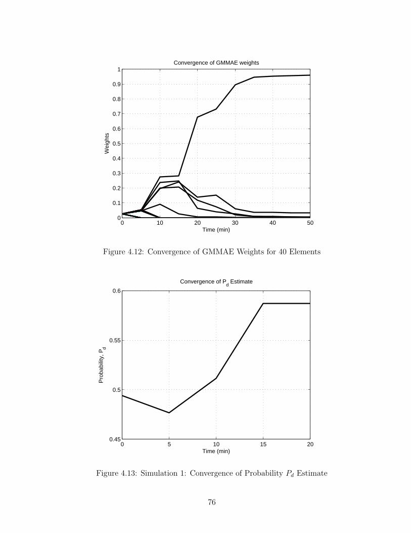
0 10 20 30 40 500
0.1
0.2
0.3
0.4
0.5
0.6
0.7
0.8
0.9
1
Time (min)
Wei
ghts
Convergence of GMMAE weights
Figure 4.12: Convergence of GMMAE Weights for 40 Elements
0 5 10 15 200.45
0.5
0.55
0.6
Time (min)
Pro
babi
lity,
Pd
Convergence of Pd Estimate
Figure 4.13: Simulation 1: Convergence of Probability Pd Estimate
76

0 5 10 15 200.05
0.1
0.15
0.2
0.25
0.3
0.35
0.4
0.45
0.5
0.55
Time (min)
Pro
babi
lity,
Pg
Convergence of Pg Estimate
Figure 4.14: Simulation 1: Convergence of Probability Pq Estimate
0 5 10 15 20 25 301.5
1.52
1.54
1.56
1.58
1.6
1.62
1.64
1.66
1.68x 10
−13
Time (min)
Pro
cess
Noi
se V
alue
s, q
Convergence of qlat
Figure 4.15: Simulation 1: Convergence of Latitudinal Process Noise Estimate
77

0 5 10 15 204.4
4.45
4.5
4.55
4.6
4.65x 10
−13
Time (min)
q long
val
ues
Convergence of qlong
Figure 4.16: Simulation 1: Convergence of Longitudinal Process Noise Estimate
between the estimated coordinates and the true coordinates relative to the 3-sigma error
bounds, Figure 4.18 displays the error between the estimated value and truth value for
a few selected points and the corresponding 3-Sigma error ellipses, Figure 4.19 displays
the output of the probability that each measurement originated from the object in track,
i.e., the output of the PDAF, and Figure 4.20 displays both the true and estimated ship
track for a small portion of the ship route.
From Figure 4.17, note the latitude and longitude errors are both well within the
3-sigma bounds, which is a good indication of the filter performance. In fact, it appears
as though the errors are even within the 1-sigma bounds (not shown in the Figure) which
indicates that the filter is performing very will with the converged values of PD, PG, qlat,
and qlong.
To emphasize the great filter performance, Figure 4.18 displays a snap shot of the
estimate-minus-truth error for 3 filter estimates. Again, the errors lie well within their
respective 3-sigma error ellipses. Figure 4.19 displays the PDF is estimating just under
78

0 5 10 15 20 25−1
−0.5
0
0.5
1Ship 1
Latit
ude
Err
ors
(Deg
)
0 5 10 15 20 25−1
−0.5
0
0.5
1
Long
itude
Err
ors
(Deg
)
Time (days)
3−Sigma Error Bounds Error
3−Sigma Error Bounds
Error
Figure 4.17: Simulation 1: Time History of Latitude and Longitude Tracking Errors
−0.6 −0.4 −0.2 0 0.2 0.4 0.6
−0.6
−0.4
−0.2
0
0.2
0.4
0.6
Latit
ude
Err
ors
(Deg
)
Longitude Errors (Deg)
Ship 1
Figure 4.18: Simulation 1: 3-Sigma Ellipses
79

0 5 10 15 20 250.93
0.94
0.95
0.96
0.97
0.98
0.99
1
Dat
a A
ssoc
iatio
n P
roba
bilit
y
Time (Days)
Ship 1
Figure 4.19: Simulation 1: Time History of Data Association
96% certainty, that the measurements originate from the target in track, never drop-
ping more than a couple percent. This is expected since there was not a lot of clutter
introduced into the simulated scenario. Figures 4.13 through 4.16 show the parameter
estimates used to tune the ship track estimator converge in approximately 15 minutes
which is fast when considered in context. Specifically, the sample period for the measure-
ments was 1 sample for every 300 seconds (5 minutes), this means that the tracker only
required 3 measurements to tune itself appropriately. Note, the GMMAE algorithm was
coded to use 5 residuals, e, in its residual bank, ǫ. Thus 5 consecutive measurements,
y, are required to fill the bank. However, the estimates converged after only 3 mea-
surements which means the residual bank didn’t have time to become fully populated.
Therefore, for this particular demonstration, using 3 residuals in the residual bank would
have yielded the same results with a smaller computational load.
The spatial dimension of the unknown parameter space is 4 (qx × qy × PD × PG) and 40
parallel filters were used in the GMMAE algorithm for the demonstration. Typically, 40
elements is not nearly enough to obtain a dense span of a 4-dimensional space. For a
reference, Figure 4.21 displays how well 100 elements fill a 2-dimensional space using a
Gaussian distribution. Nonetheless, accurate tracking performance was obtained as can
be seen in Figure 4.20.
80

2.12 2.13 2.14 2.15 2.16 2.17 2.18 2.190.49
0.5
0.51
0.52
0.53
0.54
0.55
0.56
Longitude (deg)
Latit
ude
(deg
)
Truth vs. Estimate
Figure 4.20: Simulation 1: Tracking Performance with Calculated Estimates
0 0.2 0.4 0.6 0.8 10
0.1
0.2
0.3
0.4
0.5
0.6
0.7
0.8
0.9
1
1st Paramter
2nd P
aram
ter
Spread of 100 elements in a 2−dimensional space
Figure 4.21: Gaussian distribution “Spread”
81
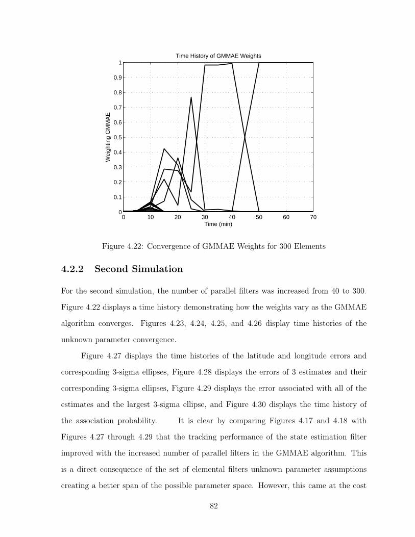
0 10 20 30 40 50 60 700
0.1
0.2
0.3
0.4
0.5
0.6
0.7
0.8
0.9
1
Time (min)
Wei
ghtin
g G
MM
AE
Time History of GMMAE Weights
Figure 4.22: Convergence of GMMAE Weights for 300 Elements
4.2.2 Second Simulation
For the second simulation, the number of parallel filters was increased from 40 to 300.
Figure 4.22 displays a time history demonstrating how the weights vary as the GMMAE
algorithm converges. Figures 4.23, 4.24, 4.25, and 4.26 display time histories of the
unknown parameter convergence.
Figure 4.27 displays the time histories of the latitude and longitude errors and
corresponding 3-sigma ellipses, Figure 4.28 displays the errors of 3 estimates and their
corresponding 3-sigma ellipses, Figure 4.29 displays the error associated with all of the
estimates and the largest 3-sigma ellipse, and Figure 4.30 displays the time history of
the association probability. It is clear by comparing Figures 4.17 and 4.18 with
Figures 4.27 through 4.29 that the tracking performance of the state estimation filter
improved with the increased number of parallel filters in the GMMAE algorithm. This
is a direct consequence of the set of elemental filters unknown parameter assumptions
creating a better span of the possible parameter space. However, this came at the cost
82
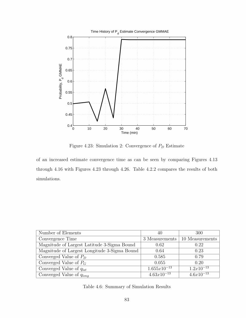
0 10 20 30 40 50 60 700.4
0.45
0.5
0.55
0.6
0.65
0.7
0.75
0.8
Time (min)
Pro
babi
lity,
Pd G
MM
AE
Time History of Pd Estimate Convergence GMMAE
Figure 4.23: Simulation 2: Convergence of PD Estimate
of an increased estimate convergence time as can be seen by comparing Figures 4.13
through 4.16 with Figures 4.23 through 4.26. Table 4.2.2 compares the results of both
simulations.
Number of Elements 40 300Convergence Time 3 Measurements 10 MeasurementsMagnitude of Largest Latitude 3-Sigma Bound 0.62 0.22Magnitude of Largest Longitude 3-Sigma Bound 0.64 0.23Converged Value of PD 0.585 0.79Converged Value of PG 0.055 0.20Converged Value of qlat 1.655x10⁻¹³ 1.2x10⁻¹³
Converged Value of qlong 4.63x10⁻¹³ 4.6x10⁻¹³
Table 4.6: Summary of Simulation Results
83

0 10 20 30 40 50 60 700.2
0.3
0.4
0.5
0.6
0.7
0.8
0.9
1
Time (min)
Pro
babi
lity,
Pg G
MM
AE
Time History of Pg Estimate Convergence GMMAE
Figure 4.24: Simulation 2: Convergence of PG Estimate
84

0 10 20 30 40 50 60 701.1
1.2
1.3
1.4
1.5
1.6
1.7x 10
−13
Time (min)
Pro
cess
Noi
se V
alue
s, q
lat G
MM
AE
Time History of qlat
Estimate Convergence GMMAE
Figure 4.25: Simulation 2: Convergence of qlat Estimate
0 10 20 30 40 50 60 704.3
4.4
4.5
4.6
4.7
4.8
4.9x 10
−13
Time (min)
Pro
cess
Noi
se V
alue
s, q
long
GM
MA
E
Time History of qlong
Estimate Convergence GMMAE
Figure 4.26: Simulation 2: Convergence of qlong Estimate
85

0 5 10 15 20−0.5
0
0.5Ship 1
Latit
ude
Err
ors
(Deg
)
0 5 10 15 20−0.5
0
0.5
Long
itude
Err
ors
(Deg
)
Time (days)
3−Sigma BoundsError
Error 3−Sigma Bounds
Figure 4.27: Simulation 2: Time History of Tracker Error with 3-Sigma Ellipses
−0.4 −0.3 −0.2 −0.1 0 0.1 0.2 0.3−0.25
−0.2
−0.15
−0.1
−0.05
0
0.05
0.1
0.15
0.2
0.25
Latit
ude
Err
ors
(Deg
)
Longitude Errors (Deg)
Ship 1
Figure 4.28: Simulation 2: Tracker Error for 3 Estimates and Corresponding 3-SigmaEllipses
86
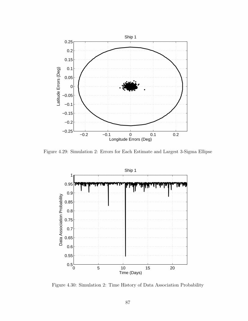
−0.2 −0.1 0 0.1 0.2−0.25
−0.2
−0.15
−0.1
−0.05
0
0.05
0.1
0.15
0.2
0.25
Latit
ude
Err
ors
(Deg
)
Longitude Errors (Deg)
Ship 1
Figure 4.29: Simulation 2: Errors for Each Estimate and Largest 3-Sigma Ellipse
0 5 10 15 200.5
0.55
0.6
0.65
0.7
0.75
0.8
0.85
0.9
0.95
1
Dat
a A
ssoc
iatio
n P
roba
bilit
y
Time (Days)
Ship 1
Figure 4.30: Simulation 2: Time History of Data Association Probability
87
Chapter 5
Conclusions and Closing Remarks
5.1 Conclusion
This work involved the development of a simulator generating ground truth data for
maritime traffic scenarios. The simulator is capable of producing data for multiple ships
at a constant or varying sampling interval of any size or statistical nature. Realistic
variations are added about a mean velocity, and the ability to stall or change the mean
velocity of a ship is implemented. When a ship stalls, the simulator sends a rescue
helicopter to repair the ship. Any of the simulator options found in Tables 4.1, 4.3,
and 4.5 can be randomly selected or mandated by the user. Contextual information is
assigned to each ship, for each scenario. Results of sample scenario simulations can be
found in Section 4.1.
The ground truth kinematics were then corrupted by sensor noise to create the effect
of measuring the ground truth with sensors. A Generalized Multiple-Model Adaptive
Estimation (GMMAE) algorithm was used to tune a Probability Data Association Filter
(PDAF) with Kalman filters (KF) by estimating the unknown parameters. The properly
tuned state estimator was used to provide estimates of the ground truth from the noisy
measurements and system model. The resulting tracking parameters converged quickly
88

and provided very good state estimates. It was shown that increasing the number of
elemental filters in the GMMAE algorithm generally increases tracking performance at
the expence of increased parameter convergence time. A demonstration can be found in
Section 4.2.
5.2 Closing Remarks
5.2.1 Ground Truth Simulator
Improvements to the ground truth simulator could come in the form of new features.
One possibility would be to allow two ships to meet at sea. This would be difficult to
implement since it would involve coordinating ship routes, velocities, and departure times
so the ships arrival times at the common location coincide. The feature would emphasize
the need for the PDAF as it would be required to decipher between the ships when they
separate.
Another improvement would be to allow a ship to change course mid-route. The dif-
ficulty here would be to splice the participating routes and merge them in such a way
so the ship does not cross land. This might require the addition of waypoints between
the route splices. The quantity, necessity, and location of these waypoints will change
depending on the participating routes and location along the routes the transition takes
place. Clearly, a generic implementation (one code that works for any combination of
routes) of this feature would be very difficult.
While adding these features it is important to be conscious of how they effect the com-
putational load. Running multiple ships with multiple features could become costly to
the computational load if care is not taken when programming. In addition to those
mentioned here, there are many features that could be added to the simulator to make
it more versatile and effective in generating scenarios to rigorously test the H2LIFT
algorithm.
89

Also, more contextual data could be added to the contextual portion of the simulation
package. Programming a graphical user interface (GUI) would be very useful if the sim-
ulator is to be used by anybody other than its creator as it would be difficult for a
user to specify scenario parameters if they are not familiar with the code. This becomes
increasingly more convenient as the number of features increases.
5.2.2 Parameter Estimation for Tuning
To improve the trackers performance even further it would be beneficial to optimize the
paramters associated with the GMMAE algorithm, namely the size, k, of the residual
bank, ǫ, and the number of parallel filters, M , used. Typically, increasing the size of the
residual bank leads to quicker convergence at the cost of increased computational load.
However, as would be expected, there is a limit to the benefits of this proceedure. For the
first demonstration presented in Section 4.2 this limit was exceeded as discussed. In some
applications a situation may arise in which the benefits of increasing k further will be
minor compared to the cost, even before the absolute limit has been reached. Similarly,
increasing the number of filters, M , utilized in the GMMAE algorithm should increase the
accuracy of the estimate at the cost of increasing computational load. The accuracy of
the estimate will increase by generating a more complete representation of the unknown
parameter solution space, increasing the likelihood that the correct parameters will be
utilized by an elemental filter. The computational load increases since the data must be
stored, and calculated, for each additional filter. Finding the optimal k and M would be
extremely beneficial in maximizing their benefits while keeping the computational load
manageable.
Also, it would be beneficial to explore different methods for assigning unknown parameter
values to the elemental filters. A Gaussian distribution was used for the demonstration in
Section 4.2 but this may not provide the best “spread” of the possible solution space. For
example, in low dimensions, the multi-dimensional Hammersley quasi-random sequence
90
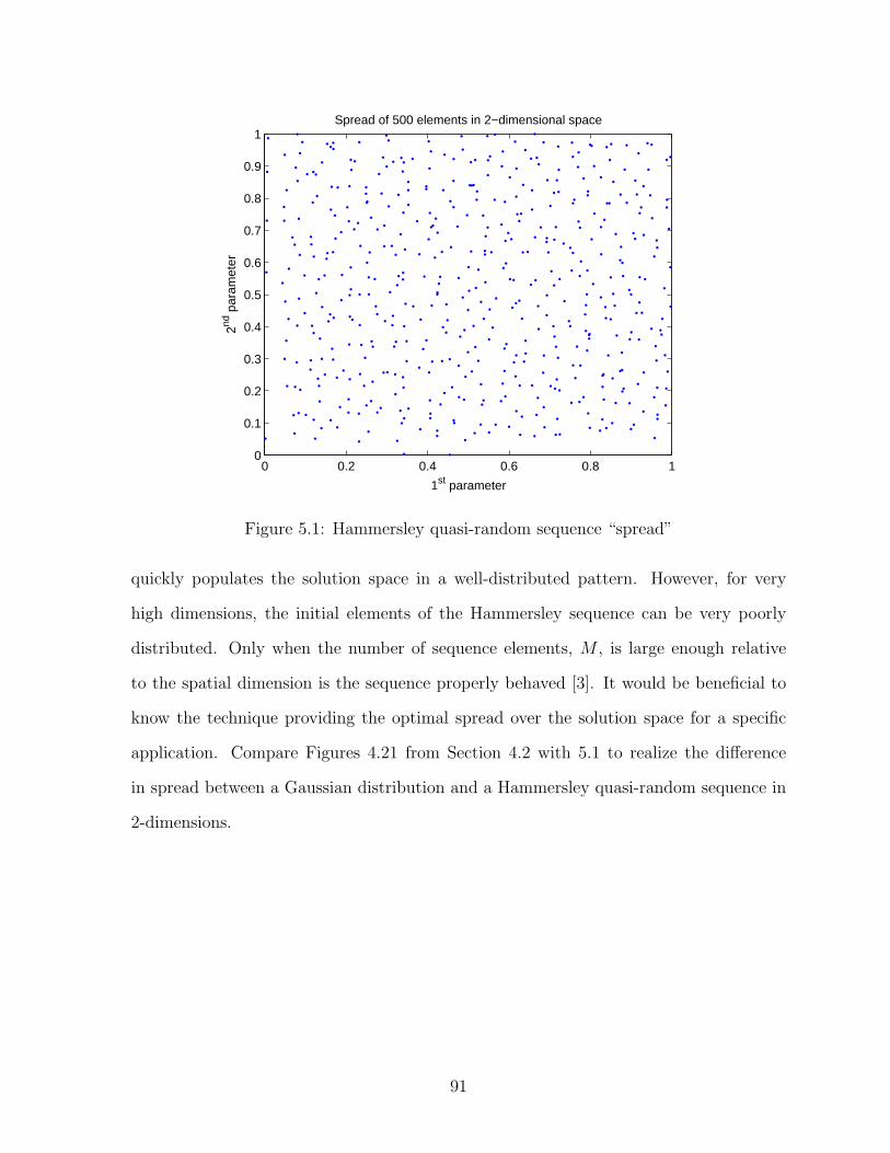
0 0.2 0.4 0.6 0.8 10
0.1
0.2
0.3
0.4
0.5
0.6
0.7
0.8
0.9
1
1st parameter
2nd p
aram
eter
Spread of 500 elements in 2−dimensional space
Figure 5.1: Hammersley quasi-random sequence “spread”
quickly populates the solution space in a well-distributed pattern. However, for very
high dimensions, the initial elements of the Hammersley sequence can be very poorly
distributed. Only when the number of sequence elements, M , is large enough relative
to the spatial dimension is the sequence properly behaved [3]. It would be beneficial to
know the technique providing the optimal spread over the solution space for a specific
application. Compare Figures 4.21 from Section 4.2 with 5.1 to realize the difference
in spread between a Gaussian distribution and a Hammersley quasi-random sequence in
2-dimensions.
91

Bibliography
[1] Bar-Shalom Y. and Tse E., “Tracking in a Cluttered Environment with ProbabilisticData Association”,Automatica,Vol.11, September 1975, pp. 451-461.
[2] R.G. Brown and P.Y.C. Hwang, Introduction to Random Signals and AppliedKalman Filtering, John Wiley and Sons, New York, NY, 2nd ed. 1992.
[3] J.L. Crassidis and Y. Cheng, “Generalized Multiple-Model Adaptive EstimationUsing an Autocorrelation Approach,” 9th International Conference on InformationFusion, Florence, Italy, July 2006, paper 223.
[4] J.L. Crassidis and J.L. Junkins, Optimal Estimation of Dynamic Systems, Chapmanand Hall/CRC Press, Boca Raton, FL, 2004. p. 285-292.
[5] J.L. Crassidis, “Sigma-point Kalman Filtering for Integrated GPS and Inertial Nav-igation” American Institute of Aeronautics and Astronautics.
[6] P. Dana “The Shape of the Earth.” 1998.http://www.ncgia.ucsb.edu/giscc/units/u015/u015.htm
[7] Gainer,Hoffman “Summary of Transformation Equations Used in Free-Flight WindTunnel Data Reduction and Analysis” Langly Research Center, 1972.
[8] P.D. Hanlon and P.S. Maybeck “Multiple-Model Adaptive Estimation Using a Resid-ual Correlation Kalman Filter Bank,” IEEE Transactions on Aerospace and Elec-tronic Systems, Vol. AES-36. No. 2, April 2000, p.393-406.
[9] D.L. Hall, and J. Llinas Handbook of Multi-Sensor Data Fusion, CRC Press, BocaRaton, FL, 2001.
[10] C.D. Ormsby, Dissertation: “Generalized Residual Multiple-Model Adaptive Esti-mation of Parameters and States” Air Force Institute of Technology, October 2003.
[11] John G. Proakis and Dimitris G. Manolakis, Digital Signals Processing: Principles,Algorithms, and Applications Fourth Edition, Prentice Hall, Upper Saddle River,New Jersey, 2007. p. 21-31.
[12] Williams, Edward “Aviation Formulary V1.42”, 6/15/2006.http://williams.best.vwh.net/avform.htm
92

[13] Williams, Edward “Rhumb Lines” 2006.http://williams.best.vwh.net/ellipsoid/node3.html
[14] S. Arulampalam, N. Gordon, and B. RisticBeyond the Kalman Filter: Particle Filters for Tracking Applications. Artech House,Boston, MA. 2004. p.179-201.
[15] R.F. Stengel, Optimal Control and Estimation Dover Publications Inc. New York,NY. 1994.
[16] The Analytical Sciences Corporation, Applied Optimal Estimation. The MIT Press,Cambridge Massachusettes. 1974.
93