development of a closed-loop strap down attitude …nasa technical memorandum 4775 development of a...

NASA Technical Memorandum 4775

Development of a Closed-Loop Strap Down Attitude System for an Ultrahigh Altitude Flight Experiment

Stephen A. Whitmore, Mike Fife, and Logan Brashear

January 1997

National Aeronautics and Space Administration

Office of Management

Scientific and Technical Information Program

1997

NASA Technical Memorandum 4775

Development of a Closed-Loop Strap Down Attitude System for an Ultrahigh Altitude Flight Experiment

Stephen A. Whitmore

Dryden Flight Research CenterEdwards, California

Mike Fife

Massachusetts Institute of TechnologyCambridge, Massachusetts

Logan Brashear

University of CaliforniaLos Angeles, California

DEVELOPMENT OF A CLOSED-LOOP STRAP DOWN ATTITUDE SYSTEM FOR AN ULTRAHIGH ALTITUDE FLIGHT EXPERIMENT

Stephen A. WhitmoreNASA Dryden Flight Research Center

Edwards, California

Mike FifeMassachusetts Institute of Technology

Cambridge, Massachusetts

Logan BrashearUniversity of CaliforniaLos Angeles, California

Abstract

A low-cost attitude system has been developed for anultrahigh altitude flight experiment. The experiment usesa remotely piloted sailplane, with the wings modified forflight at altitudes greater than 100,000 ft. Missionrequirements deem it necessary to measure the aircraftpitch and bank angles with accuracy better than 1.0° andheading with accuracy better than 5.0°. Vehicle costrestrictions and gross weight limits make installing acommercial inertial navigation system unfeasible.Instead, a low-cost attitude system was developed usingstrap down components. Monte Carlo analyses verifiedthat two vector measurements, magnetic field andvelocity, are required to completely stabilize the errorequations. In the estimating algorithm, body-axisobservations of the airspeed vector and the magneticfield are compared against the inertial velocity vector anda magnetic-field reference model. Residuals are fed backto stabilize integration of rate gyros. The effectiveness ofthe estimating algorithm was demonstrated using datafrom the NASA Dryden Flight Research Center SystemsResearch Aircraft (SRA) flight tests. The algorithm wasapplied with good results to a maximum 10° pitch and

*Aerospace Engineer, Senior Member AIAA†Graduate Student, Student Member AIAA‡Graduate StudentCopyright 1997 by the American Institute of Aeronautics and

Astronautics, Inc. No copyright is asserted in the United States underTitle 17, U.S. Code. The U.S. Government has a royalty-free license toexercise all rights under the copyright claimed herein for Governmentalpurposes. All other rights are reserved by the copyright owner.

1American Institute of Aero

bank angles. Effects of wind shears were evaluated and,for most cases, can be safely ignored.

Nomenclature

a quaternion component 1

b quaternion component 2

c quaternion component 3

d quaternion component 4

E expectation operator

F state equation matrix function, deg

airdata error covariance matrix, (ft/sec)2

inertial velocity error covariance matrix, (ft/sec)2

magnetometer error covariance matrix, (micro-Tesla)2

H altitude, ft

I identity matrix

Ip time integral of roll rate, deg

Iq time integral of pitch rate, deg

Ir time integral of yaw rate, deg

K airdata/velocity correction gain matrix

k time index

lat latitude, deg north

long longitude, deg west

GUk 1+GVk 1+

GZk 1+

nautics and Astronautics

M[.] direction cosine matrix

mi,j i, jth component of direction cosine matrix

Pk/k state error covariance matrix, previous data frame, deg2

Pk+1/k predicted state error covariancematrix, deg2

Pk+1/k+1 corrected state error covariancematrix, deg2

p roll rate, deg/sec

q pitch rate, deg/sec

Qk+1 state equation error covariancematrix, (deg/sec)2

Qx quaternion vector

||Qx|| norm of the quaternion vector

r yaw rate, deg/sec

T magnetic field reference datum,micro-tesla

t time, sec

t0 initial time, sec

U airspeed vector, ft/sec

V inertial velocity vector, ft/sec

W wind velocity vector, ft/sec

Z magnetometer measurement, micro-tesla

α angle of attack, deg

β angle of sideslip, deg

δ vector error, deg

∆t sample interval, sec

η angular velocity matrix, deg/sec

Θ attitude vector, deg

θ pitch angle, deg.

κ magnetometer correction gain matrix

Φ state transition matrix

φ bank angle, deg.

ψ yaw angle, deg.

Ω integrating factor matrix, deg

ω angular velocity vector, deg/sec

||ω|| norm of the angular velocity integral, deg

gradient vector

Superscripts and subscripts

[ ]d vertical (+ down) component ofEarth-axis vector

[ ]e east component of Earth-axis vector

[ ]k/k state estimate from previous data frame

[ ]k+1/k state estimate–based open-loop integration

[ ]k+1/k+1 state estimate after correction by magnetometer or velocity data

[ ]lat lateral component of body-axis vector

[ ]long longitudinal component ofbody-axis vector

[ ]n north component of Earth-axis vector

[ ]norm normal component of body-axis vector

[ ]T matrix transpose

state estimate after magnetometer correction

time derivative, 1/sec

Acronyms

ADC airdata computer

DFRC Dryden Flight Research Center

FCS flight control system

GPS Global Positioning System

INS inertial navigation system

MOS model output statistics

RT–FADS real-time flush airdata sensing

SRA Systems Research Aircraft

Introduction

Interest in ultrahigh altitude aircraft for atmosphericsampling and remote Earth-sensing is growing, andseveral aircraft are currently in the process of provingthe feasibility of extended duration flight to a maximumaltitude of 80,000 ft. Requirements for flights as high asan altitude of 120,000 ft have been identified. Theseflight regimes are difficult to design for, becauseresearch into low–Reynolds number, high-subsonicaerodynamics has been very limited. Although somebasic airfoils for this flight regime have been analyzedand tested in wind tunnels,1,2 fundamental data on entirevehicle aerodynamics, flight mechanics, and flightperformance are lacking.∇

[ ]

˙[ ]

2American Institute of Aeronautics and Astronautics

A preliminary design study was undertaken at theNASA Dryden Flight Research Center (DFRC) recently3

with the objective of finding a satisfactory method forachieving trimmed flight at an altitude of 100,000 ft. Thestudy for a high-altitude flight experiment examinedseveral possible techniques for achieving this objective.The study examined the feasibility of using a high-altitude balloon to tow a remotely piloted sailplane to analtitude of 100,000 ft, where it would be released andflown back to a lakeside landing on Rogers dry lakebedat Edwards Air Force Base, California.

The preliminary study concluded that the most feasibleapproach is to use a commercially available sailplane,with the wings modified for the low–Reynolds number,high-subsonic Mach number flight. For the ultrahighaltitude flight experiment, no propulsive power plantexists and this provides a low-noise environment forstudying low–Reynolds number transition phenomena.A portion of the unswept, untapered wing will serve asa test section for examining flow transition physicsunder these conditions. Figure 1 shows the ultrahighaltitude vehicle.

The current mission plan requires a nosedownballoon release, with booster rockets used to generatepseudolift to turn the vehicle from its nosedownconfiguration to level flight. After sufficient Machnumber, (approximately Mach 0.65) for free flight at

high altitudes has been achieved, the rocket pack isjettisoned. At launch and during the transitionmaneuver, accelerations along the vertical axisare substantial. Figure 2 shows a schematic of themission concept.

The unpowered a i rc ra f t wi l l co l lec t a i r fo i laerodynamics and vehicle performance data from launchto a lakebed landing at Edwards Air Force Base. Theprincipal research objectives of the ultrahigh altitudeflight experiment program are:

1. To va l ida t e h igh -a l t i t ude a i r fo i l de s ignmethodologies by measuring airfoil and vehiclecharacteristics at low Reynolds numbers andhigh subsonic Mach numbers in a low-turbulenceflight environment.

2. To establish a test bed aircraft for ultrahigh altitudeflight research.

Onboard measurements include boundary-layer velocityprofiles from total pressure rakes at several streamwiselocations, chordwise pressure distributions, theboundary-layer laminar-to-turbulent transition state,airfoil section drag (fixed wake rake), and flightmechanics data such as local angle of attack, free-streamairdata, linear accelerations, angular rates, and theaircraft attitudes. The experiment will use an onboarddata acquisition system, and data will be telemetered to


Figure 1. The ultrahigh altitude vehicle.

Top view

Test section

Airdata noseboom

Airdata noseboom

Rocket pack960644

494.35 in.

74.40 in.

271.95 in.

322.78 in.

77.70 in.

Front view

37.22 in.

40.56 in. 78.03

in.

271.95 in.322.78 in.

101.21 in.

Figure 2. Schematic of mission concept.

960645

Test maneuvers

Transition to horizontal flight

Rocket burn to achieve

horizontal flightRocket pack

release for recovery

Edward's AFB Roger's Dry Lake

Aircraft release

Aircraft landing

Ascent

Balloon launch

a ground-based recording station. Flight test maneuverswill consist of stabilized turns to achieve higher than 1-gtrim angles of attack and constant lift coefficient orMach-number descents.

To accomplish the research objectives of thisexperiment, measuring the absolute pitch and rollorientation of the aircraft to better than 1.0° and aresolution of 0.5° at the high altitudes is necessary. Forpilot navigation, measuring the vehicle heading with anabsolute accuracy of better than 5.0° with a resolutionof 1.0° is desirable. These attitude requirements resultfrom the narrow speed range allowable along the flightenvelope at these extreme altitudes. Flying too fastcauses the airfoil to develop shocks, causing potentialseparation and loss of lift. At excessive speeds, a flutterboundary may also be approached. Flying too slowlycauses the aircraft to approach stall speed. Typically, animproper attitude will translate into an unacceptablespeed change within approximately 5–10 sec. This speedchange either drives the pilot into a “speed-induced”longitudinal oscillation or reduces the pilot's attention tonothing but speed control. For this program the tolerancerequirements for the test points are restrictive, andprecise attitude information is required to ensure thatmultiple flight conditions can be met simultaneously.

The stated requirements for attitude and heading couldbe achieved using state-of-the-art inertial navigation

systems, both gimballed and strap down,4 but the costs ofthese systems are considered excessive for the ultrahighaltitude flight experiment program. Gross vehicle weightat high altitudes is of concern, and the extra weightpenalty caused by adding a full inertial navigationsystem (INS) was considered undesirable. Furthermore,the desired accuracy requirements will not be met byopen-loop integration of strap-down rate gyros.

To circumvent this problem, a simple lightweight,low-power consumption, strap-down attitude systemconcept was developed for this program and is detailedin this paper. In this system concept, body-axisobservations of the airspeed and magnetic-field vectorsare compared with the known measured inertial velocityvector and known magnetic-field vectors (in Earth-relative coordinates) to provide a “virtually inertial”reference that is used to infer an attitude error. This erroris then fed back to correct and stabilize the rate-gyrointegration. The system has the stability of gimballedattitude systems, but relies on low-cost strap-downcomponents to gather the required information. Thesystem performance is analyzed for the launch trajectoryusing Monte Carlo5 error simulations. Effects ofinstrumentation bias and random errors are analyzed.Particular attention is paid to what type of feedback isrequired to ensure full-loop closure and, hence,algorithm stability.


Data derived from the NASA Dryden SystemResearch Aircraft (SRA) flight tests6 are used todemonstrate the effectiveness of the estimatingalgorithm. The algorithm was applied to data fromseveral flights with good results achieved for up to 10°pitch and roll attitude. Reasons for estimate degradationat high attitudes are discussed. Effects of wind shears onattitude estimates are evaluated using rawindsondeweather balloon measurements.

Coordinate Definitions

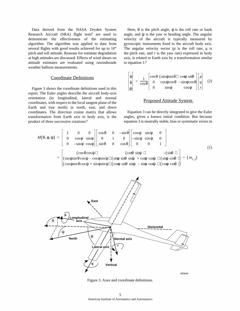
Figure 3 shows the coordinate definitions used in thisreport. The Euler angles describe the aircraft body-axisorientation (in longitudinal, lateral and normalcoordinates, with respect to the local tangent plane of theEarth and true north) in north, east, and downcoordinates. The direction cosine matrix that allowstransformation from Earth axis to body axis, is theproduct of three successive rotations:6

Here, θ is the pitch angle, φ is the roll rate or bankangle, and ψ is the yaw or heading angle. The angularvelocity of the aircraft is typically measured bygyroscopic instruments fixed to the aircraft body axis.The angular velocity vector (p is the roll rate, q isthe pitch rate, and r is the yaw rate) expressed in bodyaxis, is related to Earth axis by a transformation similarto equation 1:6

(2)

Proposed Attitude System

Equation 3 can be directly integrated to give the Eulerangles, given a known initial condition. But becauseequation 3 is neutrally stable, bias or systematic errors in

φ

θψ

1θcos

------------θcos φ θsinsin( ) φ θsincos

0 φ θcoscos φ θcossin–

0 φsin φcos

p

q

r

=


Figure 3. Axes and coordinate definitions.

960646

Vertical

North

θ

ψφ

Normal axis

r

q

pLongitudinal

axis

East

Horizontal

Lateral axis

(1)

M θ φ ψ, ,[ ]1 0 0

0 φcos φsin

0 φsin– φcos

θcos 0 θsin–

0 1 0

θsin 0 θcos

ψcos ψsin 0

ψsin– ψcos 0

0 0 1

=

θ ψcoscos( ) θ ψsincos( ) θsin( )–

φ θ ψ φ ψsincos–cossinsin( ) φ θ ψ φ ψcoscos+sinsinsin( ) φ θcossin( )φ θ ψcos φ ψsinsin+sincos( ) φ θ ψ φ ψcossin–sinsincos( ) φ θcoscos( )

mi j, = =

the rate-gyro measurements cause the integration to driftfrom the true attitudes as a function of time. Thus, loopclosure is required to get a stable attitude measurement.For conventional inertial systems, a stable reference isprovided by a gimballed platform. Payload limitations ofthe vehicle and large vertical accelerations at launchmake this approach unfeasible for this ultrahigh altitudeflight experiment, as described earlier.

The system proposed for the ultrahigh altitude vehicleuses strap-down components that are low in cost, do notrequire a stable member to perform the integration, andare insensitive to large accelerations in the vertical axes.Body-axis angular rates are integrated and stabilizedusing measurements of airspeed, inertial velocity, andmagnetic-field vectors. As will be shown in the resultsand discussion section, two vector measurements,magnetic field and velocity, are required to achievecomplete three-attitude stability. The approach compares

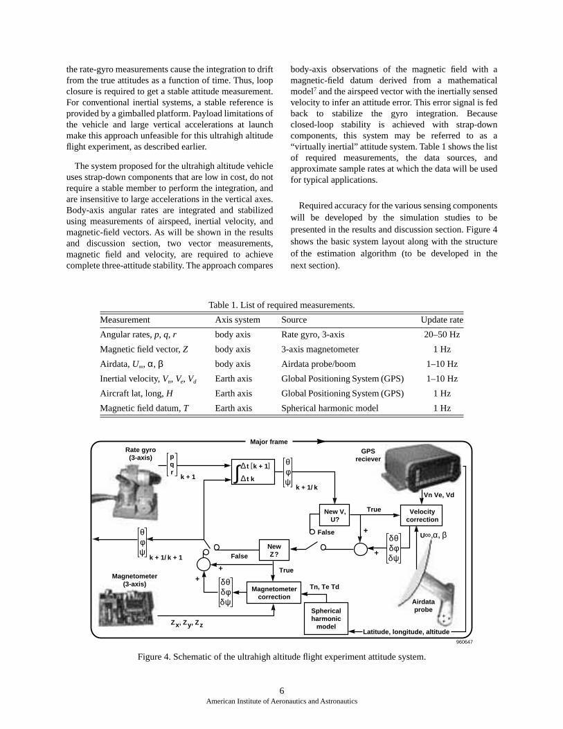
body-axis observations of the magnetic field with amagnetic-field datum derived from a mathematicalmodel7 and the airspeed vector with the inertially sensedvelocity to infer an attitude error. This error signal is fedback to stabilize the gyro integration. Becauseclosed-loop stability is achieved with strap-downcomponents, this system may be referred to as a“virtually inertial” attitude system. Table 1 shows the listof required measurements, the data sources, andapproximate sample rates at which the data will be usedfor typical applications.

Required accuracy for the various sensing componentswill be developed by the simulation studies to bepresented in the results and discussion section. Figure 4shows the basic system layout along with the structureof the estimation algorithm (to be developed in thenext section).


Figure 4. Schematic of the ultrahigh altitude flight experiment attitude system.

Table 1. List of required measurements.

Measurement Axis system Source Update rate

Angular rates, p, q, r body axis Rate gyro, 3-axis 20–50 Hz

Magnetic field vector, Z body axis 3-axis magnetometer 1 Hz

Airdata, U∞, α, β body axis Airdata probe/boom 1–10 Hz

Inertial velocity, Vn, Ve, Vd Earth axis Global Positioning System (GPS) 1–10 Hz

Aircraft lat, long, H Earth axis Global Positioning System (GPS) 1 Hz

Magnetic field datum, T Earth axis Spherical harmonic model 1 Hz

Rate gyro(3-axis)

Magnetometer(3-axis)

Major frame

Zx, Zy, Zz

GPSreciever

Vn Ve, Vd

Tn, Te Td

False

True

False

True

Airdataprobe

++

+

+

Latitude, longitude, altitude

Sphericalharmonic

model

U∞,α, β

δθδφδψ

δθδφδψ

k + 1

pqr

k + 1/ k + 1

θφψ

k + 1/ k

θφψ

New V,U?

NewZ?

∆ t [k + 1]

∆ t k∫

Velocitycorrection

Magnetometercorrection

960647

Development of the Estimation Algorithm

This section develops a closed-loop estimationalgorithm for the strap-down (nongimballed) attitudesystem. Measurement errors from the independentsystems, (such as airspeed, magnetometer, inertialvelocity, and angular rates) are assumed to beuncorrelated. The algorithm emulates the form of theKalman filter, modified for asynchronously arriving data(the fundamental Kalman assumes that all data from thevarious measurement sources arrive simultaneously).For the types of disparate data sources to be used forultrahigh altitude flight systems (for example,magnetometer, Global Positioning System (GPS),analog), a frame-by-frame algorithmic approach is toorestrictive. To circumvent this difficulty, the estimationalgorithm is implemented as a two-step predictor/corrector filter where the prediction-step (quaternionintegration of the rate-gyro data) is performed at a fixedrate, typically 25–50 Hz, and the correction step isperformed whenever fresh velocity and magnetometerdata are available, typically 1–10 Hz.

Quaternion Formulation of the Rate Integrator

As is typical of all modern INS systems, to eliminateproblems with infinite angular rates caused by thenosedown initial attitude at launch, the estimationalgorithm formulates the problem in terms of quaternionparameters.4,8 In the quaternion transformation theorientation is written as a 4-space vector with themagnitude being constrained to always be unity. Usingmi,j for the elements of the direction cosine matrix (eq. 2),then the quaternions can be evaluated by

(3)

This quaternion substitution transforms the kinematicsequations (eq. 2) to a linear form,

(4)

and the direction cosine matrix becomes

(5)

The transformation from quaternions to Euler angles is

(6)

Solution of the Integrating Equation

Equation 4 is solved by the integrating factor9 method:

(7)

The integrating factor is

(8)

where

(9)

and can be written in closed form by expanding theexponential in a Taylor series9

(10)

and noting that

(11)

Qx

a

b

c

d

≡

m23 m32–

4d------------------------

m31 m13–

4d------------------------

m12 m21–

4d------------------------

12--- 1 m11 m22 m33+ + +

Qx2

1=⇒=

a

b

c

d

12---

0 r q– p

r– 0 p q

q p– 0 r

p– q– r– 0

a

b

c

d

q t( )⇒ ω p q r, ,( ) q t( )= =

Mθφψ

a2

d2

b2

– c2

–+ 2 ab cd+( ) 2 ac bd–( )

2 ab cd–( ) b2

d2

a2

– c2

–+ 2 bc ad+( )

2 ac bd+( ) 2 bc ad–( ) c2

d2

a2

– b2

–+

=

θsin 2 bd ac–( )=

ψtan 2 ab cd+( )

2 a2

d2

+( ) 1–-----------------------------------=

φtan 2 bc ad+( )

2 c2

d2

+( ) 1–----------------------------------=

Qx t( ) e η p q r, ,( ) dt Qx t0( )t0

t

∫=

e η p q r, ,( ) dtt0

t

∫ e12---

0 r q– p

r– 0 p q

q p– 0 r

p– q– r– 0

dtt0

t

∫=

e=

0 Ir 2⁄ Iq 2⁄– I p 2⁄

Ir 2⁄– 0 I p 2⁄ Iq 2⁄

Iq 2⁄ I p 2⁄– 0 Ir 2⁄

I p 2⁄– Iq 2⁄– Ir 2⁄– 0

eΩ p q r t, , ,( )≡

Ir

2---- r t( )dt

2--------------

Iq

2---- q t( )dt

2--------------

I p

2----- p t( )dt

2---------------

t0

t

∫≡,t0

t

∫≡,t0

t

∫≡

eΩ

I Ω Ω2

2------- Ω3

3!------- …+ + + +=

Ω2 I p 2

Iq 2

Ir 2

+ +

4----------------------------------- ω

2--------

2I–≡–=


The matrix, I, is the identity matrix. Collecting termsand simplifying gives

(12)

resulting in the homogeneous linear equation

(13)

The integrator is made recursive over a small timestep, ∆t, using angular rates averaged over the interval

(14)

Equation 14 is the “one-step prediction equation,” andis always norm preserving. That is, the quaternionmagnitude will always be equal to unity, and one doesnot have to re-normalize the quaternion values after eachintegration cycle. This ensures greater numericalaccuracy and is a unique result not published innavigation literature.

Correction of Integrated Data

At the end of each integration frame, the algorithmcorrects for drift instabilities by using the differencesbetween the magnetic-field and airspeed vectors,measured in body axes and the magnetic-field datum andinertial velocity vector, measured in Earth-relative axes.A particular state error correction is performed onlywhen a fresh measurement is available. To allow for thisasynchronous operation, the correction step ispartitioned into two parts: a magnetometer correction,and a velocity correction.

The magnetometer correction is performed first. Inthis step, differences between the observed and expectedmagnetic-field vector are fed back to stabilize the open-loop integration,

(15a)

Here, the matrix κk+1 is a “Kalman-style” gain matrix,Tk+1 is the magnetic-field reference datum in Earthcoordinates, and Zk+1 is a three-axis magnetometermeasurement in body axis.

The vector

is the predicted state estimate based on open-loopintegration over one integration cycle, and the vector

is the state estimate resulting from the magnetic-fieldvector correction. The matrix M[.] is the transformationmatrix for rotation from Earth–to–body axis based on thepredicted state parameters

(15b)

If no fresh magnetic-field data are available, then themagnetometer correction step is ignored.

After the magnetometer update, the result is correctedusing newly acquired velocity data (if available):

(16)

Here, the matrix Kk+1 is the gain matrix, Uk+1 is thebody-axis airspeed vector, Vk+1 is the inertial velocitymeasurement (from the GPS), and Wk+1 is the vectorrepresenting the local atmospheric winds. As with theprevious correction, the vector

is the new state estimate. As with the magnetometercorrection step, if fresh velocity data are unavailable,then the velocity correction step is ignored.

With no direct measurement of the vehicle attitudesavailable, the wind terms in equation 16 are difficult tosense in real time. Conceptually, the wind vector can beestimated by comparing inertial velocities to airdata

eΩ ω

2-------- I

2ω

-------- ω2

--------Ω Φ t t0,( )≡sin+cos=

Qx t( ) Φ t t0,( )Qx t0( )=

Qxk 1+Φk 1 k,+ Qxk

=

θφψ k 1 k 1+⁄+

θφψ k 1 k⁄+

κk 1+ Zk 1+ Mθφψ k 1 k⁄+

Tk 1+–+=

θφψ k 1 k⁄+

θφψ k 1 k 1+⁄+

zlong

zlat

znorm

Mθφψ k 1 k⁄+

Tn

Te

Td

=

θφψ k 1 k 1+⁄+

θφψ k 1 k 1+⁄+

=

Kk 1+ Uk 1+ Mθφψ k 1 k 1+⁄+

Vk 1+ Wk 1++ –+

θφψ k 1 k 1+⁄+


measurements. But because the inertial velocity vector issensed in the Earth-relative axis system and the airdatavelocity vector is sensed in the body-axis, the vehicleattitudes are implicit in the velocity comparison.This implicitness requires that the attitudes and windsare iteratively estimated. In the iterative method,the attitudes would first be estimated assuming nowinds. Using these attitude estimates, the winds areestimated from the differences between the inertialand airdata velocity vectors. The attitudes are thenreevaluated iteratively using the estimated winds.Two primary difficulties exist with the iterative method.First, such a complex iterative scheme is very difficultto run in real time; and second, because the attitudeequations are highly nonlinear, no guarantee existsthat the iterative equations will converge. Thisnonlinearity makes the iterative algorithm unsuitable forflight-critical navigation.

For simplicity, the winds will either be measured byweather balloon or ignored altogether. As described laterin the Results and Discussion section, the winds cangenerally be measured with good steady-state accuracyby rawindsonde weather balloons,10 but these data aresubject to diurnal (time) and spatial variation errors.Ignoring the winds, or using wind measurements withlarge errors, will result in biases in the attitude estimates;however, these errors will not affect the stability of thealgorithm. The effects of wind shear will be illustrated inthe Results and Discussion section using data from theSRA flight tests.

Computation of the Gain Matrixes

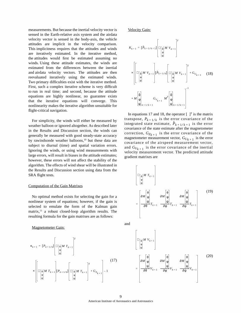
No optimal method exists for selecting the gain for anonlinear system of equations; however, if the gain isselected to emulate the form of the Kalman gainmatrix,11 a robust closed-loop algorithm results. Theresulting formula for the gain matrixes are as follows:

Magnetometer Gain:

(17)

Velocity Gain:

(18)

In equations 17 and 18, the operator [ ]T is the matrixtranspose, is the error covariance of theintegrated state estimate, is the errorcovariance of the state estimate after the magnetometercorrection, is the error covariance of themagnetometer measurement vector, is the errorcovariance of the airspeed measurement vector,and is the error covariance of the inertialvelocity measurement vector. The predicted attitudegradient matrixes are

(19)

and

(20)

κk 1+ Pk 1 k⁄+[ ] ∇ θφψ

M Tk 1+

T

=

∇ θφψ

M Tk 1+ Pk 1 k⁄+[ ] ∇ θφψ

M Tk 1+

T

GZk 1++× 1–

Kk 1+ Pk 1 k 1+⁄+[ ] ∇ θφψ

M Vk 1+

T

=

∇ θφψ

M Vk 1+ Pk 1 k⁄+[ ] ∇ θφψ

M Vk 1+

T

GUk 1++×

Mθφψ k 1 k 1+⁄+

GVk 1+ M

Tθφψ k 1 k 1+⁄+

1–

+

Pk 1+ k⁄Pk 1 k 1+⁄+

GZk 1+GUk 1+

GVk 1+

∇ θφψ

M Tk 1+

∂Mθφψ

∂θ------------------Tk 1+

∂Mθφψ

∂φ------------------Tk 1+

∂Mθφψ

∂ψ------------------Tk 1+=

∇ θφψ

M Vk 1+

∂Mθφψ

∂θ------------------Vk 1+

∂Mθφψ

∂φ------------------Vk 1+

∂Mθφψ

∂ψ------------------Vk 1+=


The forms of the gain matrixes determine thatvery little correction occurs to the integrated state ifthe measurement (magnetometer and velocity vectors)covariances are large. Conversely, if the integrationerror covariance is large, then the filter applies alarge correction based on the measured data. In thiscase, the gradient is a sensitivity matrix describinghow much correction should be applied to the integratedstate vector based on the magnetic-field and velocity-vector feedbacks.

Computation of the Error Covariance Matrices

A mechanism for evaluating and propagating the errorcovariances from one data frame to the next must bedeveloped for the filter to be complete. Again, because ofthe highly nonlinear nature of the problem, an exactexpression cannot be developed for the covariancepropagations. Instead, approximate expressions arederived from the equations of motion, linearized aboutthe state estimate from the previous data frame.

The error covariance of the integrated state estimate isderived indirectly from the basic kinematics equations.Equation 2 is written here in vector form as

(21)

where

(22)

By integrating equation 22 over one data frame usingexplicit12 differencing to approximate the timederivative, the result is

(23)

Taking perturbations and collecting terms gives thefollowing error equation:

(24)

Defining the covariance matrices

(25)

and assuming that the current input error δωk isuncorrelated with the current state error δΘk/k, then theprediction error covariance update equation can bewritten approximately as

(26)

After the correction steps are performed, the errorcovariances of the state estimates are reevaluated in asimilar manner by propagating the error throughcorrection equations. The resulting propagationequations are as follows:

magnetometer covariance update:

(27)

velocity covariance update:

(28)

Equations 2, 4, 15, 7, 27, 18, 20, 28, 19, 21, and 29 arethe collected algorithm equations. The equation set isrepeated recursively until the data stream is exhausted. Ifat a particular time a new measurement is unavailable,then that correction step is not performed, and the stateand covariance matrixes remain unchanged. Figure 4shows the basic algorithm structure as discussed earlier.

Θ F Θ[ ]ω=

Θθφψ

ω,p

q

r

and,= =

F Θ[ ] 1θcos

------------θcos φ θsinsin φ θsincos

0 φ θcoscos φ θcossin–

0 φsin φcos

=

Θk 1 k⁄+ Θk k⁄ ∆t F Θk k⁄[ ]ωk +=

δΘk 1 k⁄+ I ∆t ∇Θ F Θk k⁄[ ]ωk( )+[ ]δΘk k⁄=

∆t F Θk k⁄[ ]δωk+

Pk 1 k⁄+ E δΘk 1 k⁄+ δΘk 1 k⁄+T ,=

Pk k⁄ E δΘk k⁄ δΘk k⁄T ,=

Qk E δωkδωkT

etc.,=

Pk 1 k⁄+

I ∆t ∇Θ F Θk k⁄[ ]ωk( )+= Pk k⁄ I ∆t ∇Θ F Θk k⁄[ ]ωk( )+T

∆t2F Θk k⁄[ ]QkF

T Θk k⁄[ ]+

Pk 1 k 1+⁄+ I Kk 1+ ∇ θφψ

M Tk 1+– Pk 1 k⁄+=

Pk 1 k 1+⁄+ I Kk 1+ ∇ θφψ

M Vk 1+– Pk 1 k⁄+=


Results and Discussion

This section presents results that evaluate theperformance of the estimating algorithm. The systemperformance is analyzed for the ultrahigh altitude flightexperiment launch trajectory using Monte Carlo errorsimulations. The estimation algorithm is alsodemonstrated using flight data derived from the SRAflight tests. Effects of wind shears on the attitudeestimate are evaluated using these data.

Six-Degree- of-Freedom Monte Carlo Errors Analyses

The performance of the attitude estimation algorithmwas evaluated by Monte Carlo error simulationsgenerated using the NASA Dryden six-degree-of-freedom piloted simulation for the ultrahigh altitudeaircraft. Typical balloon-release maneuvers were flownto give representative trajectories for the vehicle launch.These data were then corrupted by bias and randomerrors, magnetic compass lags, and measurementlatencies to simulate the types of real-worldmeasurement errors that would be encountered. Biaserrors were introduced into the various measurements atthe beginning of each simulation run using a randomnumber generator and a specified bias standarddeviation. When the values for the biases were set for aparticular data run, they were held constant throughoutthe remainder of the run. Random errors were generatedin a similar manner, except these errors were added to thevarious data sources at each data frame.

The effects of systematic errors such as compass lagsor data latencies were evaluated using various filters thatmodeled these effects. Also, the piloted launch wasrepeated several times with different initial launchconditions for heading and initial angular rates.Magnetometer data were generated using a sphericalharmonic model of the Earths magnetic field7 with theaircraft longitude, latitude, and altitude as inputs to themagnetic-field model. These data were then rotated tobody axes and corrupted with bias, random, and compass

lag errors. The compass lag errors were added tosimulate the induced errors caused by crossing lines ofmagnetic flux as the aircraft changes pitch attitude orheading attitude. Relative to the expected magnetometererrors, the magnetic-field reference model is extremelyaccurate, and the resulting reference data are assumed tobe known without error.

For each simulation run, the corrupted data were usedby the attitude-estimating algorithm to generate Eulerangle estimates. Comparisons of the estimated attitudeangles with the actual attitude angles (from thesimulation) give quantitative measures of the systemperformance. To obtain ensemble averages of the errorsinduced by random and bias error components, thesimulations were run repeatedly and model outputstatistics (MOS) were generated. The measurementrequirements to achieve the 1.0° attitude accuracy of theprogram were determined by this method. Particularattention was paid to determine when a given setof measurements provided closed-loop stability tothe algorithm.

Figures 5 through 9 show results of a typicalsimulation run. Figure 5 shows the basic launchtrajectory, where time histories of the airdata parameters(airspeed, angle of attack, altitude, and the roll, pitch,and yaw rates) are presented. Figure 5 shows theuncorrupted and corrupted data that was actually used toperform the analyses. Table 2 presents the bias andrandom error standard deviations that were used in thissimulation run.

The integration is performed at a rate of 25 samples/sec, the magnetometer data are assumed to be available5 times/sec, and the velocity data are obtained every 1sec. The corrupted magnetometer data were lagged usinga second-order filter with a time constant of 1.25 sec, anda damping ratio of 0.8.

Figure 6 shows a comparison of the true Euler angleswith the attitudes derived from open-loop integration ofthe corrupted angular-rate data. Clearly, the integration is


Table 2. Bias and random error standard deviations of measurement data.

Measurement Bias error Random error

Angular rates, p, q, r –0.81, 0.72, -0.77 deg/sec ±0.25 deg/sec

Magnetic field vector, Z –1.7, 1.1, 0.74 percent ±5.0%

Airdata, V∞, α, β –2.2 ft/sec, –0.14°, –0.15° ±5.0 ft/sec, ±0.25°, ±0.25°Inertial velocity, Vn, Ve, Vd –1.3, –2.6, –3.7 ft/sec ±3.0 ft/sec

Magnetic field datum, T no error no error


(a) Airspeed.

(b) Angle of attack.

(c) Altitude.Figure 5. Ultrahigh altitude flight experiment launch trajectory time histories.

700

600

500

400

300

200

100

0

–100

Airspeed, ft/sec

0 12 24 36 48 60 72 84 96 108 120Time, sec

960648

True airspeed

Noise corrupted airspeed

2.00

7.00

5.75

4.50

3.25

.75

–.50

–1.75

–3.00

Angle of attack,

deg

0 12 24 36 48 60 72 84 96 108 120Time, sec

960649

True angle of attack Noise corrupted angle of attack

102,000

99,500

97,000

94,500

92,000

104,500

107,000

109,500

112,000

Altitude, ft

0 12 24 36 48 60 72 84 96 108 120Time, sec

960650

True altitude

Noise corrupted altitude


(d) Roll rate.

(e) Pitch rate.

(f) Yaw rate.Figure 5. Concluded.

0

.375

.750

1.125

1.500

–1.500

–1.125

–.750

–.375

Roll rate, deg/sec

0 12 24 36 48 60 72 84 96 108 120Time, sec

960651

True roll rate

Noise corrupted roll rate

2

0

4

6

8

–8

–6

–4

– 2

Pitch rate, deg/sec

0 12 24 36 48 60 72 84 96 108 120Time, sec

960652

True pitch rate

Noise corrupted pitch rate

0

.375

.750

1.125

1.500

–1.500

–1.125

–.750

–.375

Yaw rate, deg/sec

0 12 24 36 48 60 72 84 96 108 120Time, sec

960653

True yaw rate

Noise corrupted yaw rate


(a) Pitch angle.

(b) Bank angle.

(c) Heading angle.Figure 6. Launch Euler angle comparisons: true attitudes versus open-loop estimates.

0 12 24 36 48 60 72 84 96 108 120

30

15

0

– 15

– 30

– 45

– 60

– 75

– 90

Pitch angle,

deg

Time, sec960654

True angle Open-loop estimate

0 12 24 36 48 60 72 84 96 108 120

20

10

0

– 10

– 20

– 30

– 40

– 50

– 60

Bank angle,

deg

Time, sec960655


0 12 24 36 48 60 72 84 96 108 120

70

60

50

40

30

20

10

0

–10

Heading angle,

deg

Time, sec960656


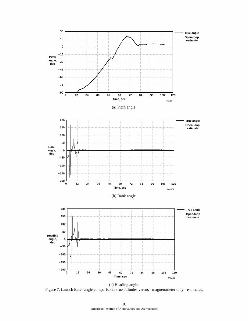
unstable, and the three attitude angles wander from thetrue attitudes. Figure 7 shows similar comparisons,except the attitudes have been estimated using themagnetometer data for partial system loop closure.Clearly, the performance is now much better, havingonly small drifts on pitch and bank angles and a moresubstantial drift in the heading angle. The system is notyet stable, and the stringent requirements of the ultrahighaltitude flight experiment are not met.

Figure 8 shows the same comparisons, except nowonly the airspeed and inertial velocity differences havebeen used to partially close the loop. Again, the system isfairly stable in the pitch and yaw axes, but drifts badly inthe roll axis. Because airdata provided only smallamounts of information regarding the roll of the vehicle,this result is expected. Figure 9 shows the Euler anglecomparisons where magnetometer, airspeed and velocitydifferences have been used for loop closure. Here, thesystem loop has been completely closed, and thecomputations are stable in all three axes. Almostimmediately after launch, the estimates converge tothe true values. The error equations have beenfully stabilized.

Clearly then both the magnetometer and airspeed andinertial velocity stabilizations are required for acompletely reliable system. Based on the accuracy andresolution specifications stated earlier, the Monte Carloanalyses MOS were used to assess the maximum biasand random errors allowable to meet the ultrahighaltitude flight program requirements. Table 3 showsestimates of these data for the fully stable system.Measurement latency limitations have yet to beestablished, but based on the simulation runs, theserequirements are very relaxed and can be easily achievedwith conventional instrumentation methods.

The key to achieving this instrumentation robustness isin using the two independent attitude references, themagnetic and velocity-vector fields, to completely closethe loop on the error equation so that a stable set of(linearized) error equations results. Even in the presence

of sizable measurement biases, the system errors will notgrow as a function of time.

Evaluation of Attitude-Estimating AlgorithmUsing Systems Research Aircraft Flight Data

As mentioned in the introduction, the effectiveness ofthe estimating algorithm under real flight conditions willbe demonstrated using data derived from the SRA flighttests.13 The SRA is an F/TF-18 aircraft and is an earlymodel equipped with a high-quality mechanical-gyroINS.14 The attitudes from this INS system are used as thereference standard, or “truth model,” for this analysis.Estimated accuracies of the INS attitudes are betterthan ±0.25° in pitch and bank angle and ±0.5° in yawangle. Other outputs from the INS include linearaccelerations, angular rates, inertial velocity, flightpath and ground track, and aircraft latitude, longitude,and altitude.

The F/TF-18 is also equipped with an additional set ofangular rate sensors that are used as feedback sensors forthe flight control system (FCS).14 The FCS rate gyros,although efficient dynamically, are subject to small biaserrors and systematic drifts. Because FCS rate gyros areindependent from the INS (although clearly not as highin quality as the INS angular rate outputs), the FCS datawere used for the roll, pitch, and yaw rate inputs to theattitude algorithm. This use of FCS rate gyros avoids anyperceived incestuousness in the analysis. Estimatedaccuracies of the rate data are better than ±0.1 deg/sec forbias error, and ±0.2 deg/sec for random error.

Two airdata systems are available on the SRA: theship system airdata from the airdata computer (ADC),14

or the research real-time flush airdata sensing(RT–FADS) system. At low angles of attack, theRT–FADS system and ADC have equivalent levels ofaccuracy. At greater than 32° angle of attack, the ADCsystems stop operating, whereas the RT–FADS systemhas been demonstrated to be accurate to a maximum48° angle of attack.13 For this reason, the RT–FADSairdata were used in this analysis. Estimated accuracies


Table 3. Maximum bias and random errors allowable for the measurement data.

Measurement Bias error Random error

Angular rates, p, q, r ±0.1, ±1.50, ±2.5 deg/sec ±2.0 deg/sec

Magnetic field vector, Z ±10.0 percent ±20 percent

Airdata, U∞, α, β ±10.0 ft/sec, —0.4°, ±0.4° ±15.0 ft/sec, ±0.5°, ±0.5°Inertial velocity, Vn, Ve, Vd ±10.0 ft/sec ±15.0 ft/sec


(a) Pitch angle.

(b) Bank angle.

(c) Heading angle.Figure 7. Launch Euler angle comparisons: true attitudes versus - magnetometer only - estimates.

–30

–15

0

15

30

–75

–60

– 45

–90

Pitch angle, deg

0 12 24 36 48 60 72 84 96 108 120Time, sec

960657

True angle

Open-loop estimate

–150

– 200

–100

– 50

0

50

100

150

200

Bank angle, deg

0 12 24 36 48 60 72 84 96 108 120Time, sec

960658

True angle

Open-loop estimate

–150

– 200

–100

– 50

0

50

100

150

200

Heading angle, deg

0 12 24 36 48 60 72 84 96 108 120Time, sec

960659

True angle

Open-loop estimate


(a) Pitch angle.

(b) Bank angle.

(c) Heading angle.Figure 8. Launch Euler angle comparisons: true attitudes versus airdata only estimates.

0

15

30

–75

–60

–45

–30

–15

–90

Pitch angle,

deg

0 12 24 36 48 60 72 84 96 108 120Time, sec

960660


20

40

60

–80

–60

–40

–20

0

–100

Bank angle,

deg

0 12 24 36 48 60 72 84 96 108 120Time, sec

960661


50

60

70

0

10

20

30

40

–10

Heading angle,

deg

0 12 24 36 48 60 72 84 96 108 120Time, sec

960662



(a) Pitch angle.

(b) Bank angle.

(c) Heading angle.Figure 9. Launch Euler angle comparisons: true attitudes versus magnetometer estimates.

0

15

30

–75

–60

–45

–30

–15

–90

Pitch angle,

deg

0 12 24 36 48 60 72 84 96 108 120Time, sec

960663


100

150

200

–150

–100

–50

0

50

–200

Bank angle,

deg

0 12 24 36 48 60 72 84 96 108 120Time, sec

960664


100

150

200

–150

–100

–50

0

50

–200

Heading angle,

deg

0 12 24 36 48 60 72 84 96 108 120Time, sec

960665


of the RT–FADS system13 are 3–5 ft/sec in airspeed,and ±0.25° in angle of attack, and angle of sideslip. Thesystem has been tested and found to be reliable to amaximum of Mach 1.60.

Again, to avoid any perceived incestuousness in theanalysis, the inertial velocity measurements from theINS were not used in this analysis. Because, the SRAwas not equipped with a GPS, inertial velocity estimateswere obtained using C-band radar tracking data. In thisprocedure, space-positioning data are numericallydifferentiated to give velocities relative to the Earth-axissystem. For radar elevation angles greater than 10°, therandom accuracies in the radar velocity data are believedto be approximately ±4–8 ft/sec and are of necessityunbiased (because of the numerical differentiation).13

Time skews resulting from the differentiating filterswere removed before processing the data in theattitude algorithm. Although not truly a strap-downmeasurement, these C-band data are a goodapproximation of the type of data that would be acquiredby an onboard GPS system.

Three-axis magnetic-field measurements were notavailable on the SRA vehicle. Instead, the F/TF-18 SRAhas a single-axis magnetic compass available as a part ofthe cockpit instrumentation, and this instrument wasused to generate a pseudo 3-axis magnetometer data set.The estimated compass accuracy is ±1° in bias, and±5° random. For a given latitude and longitude, thereference magnetic-field datum vector (from thespherical harmonic model) was rotated about the verticalaxis until the vector angle from magnetic north matchedthe compass heading. Similarly, a pseudo pitch anglewas generated from the radar flightpath angle and theangle-of-attack measurement. This angle was used torotate the magnetic-field vector to the proper pitchattitude. As no data for bank angle were availableindependent of the INS measurements, the magnetic-field vector was not rotated about the roll axis. To preventerroneous data corrections caused by this lack ofroll information, the magnetometer correction wasperformed only when the absolute value of the predictedbank angle was less than 10°. This lack of bank angleinformation at high roll angles presents a less-than-idealscenario for the estimating algorithm.

Flight 540 Results

Results from SRA flight 540 will now be presented.Calculations are performed from takeoff to landing andare typical of results from other SRA flights. All of thedata used are from the sources described in the previoussection. Figure 10 shows time histories of the airdataparameters airspeed, angle of attack, and altitude, andthe angular-rate parameters roll, pitch and yaw rate.

As with the attitude analyses presented earlier in thepaper, figures 11 and 12 show comparisons of theestimated attitudes and INS attitudes. Figure 11 shows acomparison of the INS-derived Euler angles with theattitudes derived from open-loop integration. The rate-gyro integration was performed at a rate of 25 samples/sec. Clearly, the open-loop estimates are unstable, andthe Euler components wander around the INS valuesthroughout the flight. Figure 12 shows attitudecomparisons where corrections have been applied tocompass, velocity, and airdata once every second tostabilize the rate-gyro integration. As predicted bythe earlier Monte Carlo simulations, the error equation isstabilized and no significant long-term attitudedrift occurs.

Figure 13 shows a subset of the data shown infigure 12, but with an expanded time scale to moreclearly show the level of agreement between the INS andestimated attitudes. For bank angles less than 10°, theagreements are within the specified requirements for thisexperiment (errors less than ±0.5° in pitch axis and ±1.0°in roll). For roll angles larger than 10°, the estimatesdegrade in both pitch and roll axes, with pitch angleerrors as large as –3° and roll angle errors as largeas –10°. As mentioned previously the deviation fromINS attitudes is not surprising given that for this analysisno magnetic field correction is applied for bank angles atgreater than 10°. The ultrahigh altitude flight experimentheading accuracy requirement of ±5° is met throughoutthe entire flight. Analyses of data from other SRA flightshave produced similar results.

The Effects of Wind Shear on the Attitude Estimates

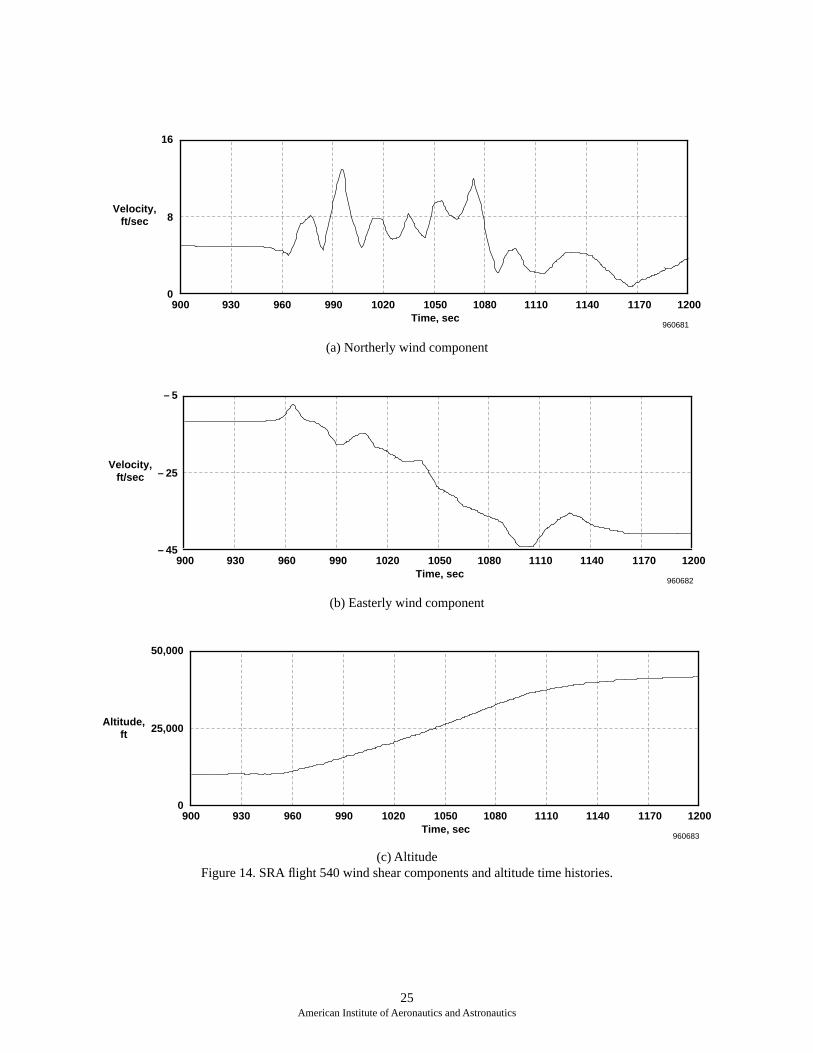
As mentioned earlier, the wind velocity will betypically ignored by the ultrahigh altitude flightexperiment algorithm because measuring in real time isdifficult. In the presence of significant wind shears, theresult of ignoring the winds is a bias or systematic errorin the attitude estimates. Figures 14 and 15 show theeffect of wind shear using data from the SRA flight 540.For this flight, the atmospheric winds were measuredbefore and after flight using rawinsonde11 weatherballoon soundings, interpolated as a function of time tominimize the effects of diurnal variations in the winds.

During the flight, the vehicle rapidly climbed from analtitude of 10,000 ft to an altitude of 40,000 ft, resultingin a large change in the easterly component of the wind.Figure 14 shows time histories of the horizontal windcomponents and altitude. The full feed back (magnetic-field, airdata, and velocity) attitude-estimating algorithmwas run for this segment of data with and withoutthe measured winds being included in the computations.



(a) Airspeed.

(b) Angle of attack.

(c) Altitude.Figure 10. SRA flight 540 time history, takeoff to landing.

160012008004000 2000 2400 2800 3200 3600 4000

1100

600

100

Airspeed, ft/sec

Time, sec960666

50

25

0

Angle of attack,

deg

16001200800400 2000 2400 2800 3200 3600 4000Time, sec

960667

50,000

25,000Altitude,

ft

160012008004000 2000 2400 2800 3200 3600 4000Time, sec

960668


(d) Roll rate.

(e) Pitch rate.

(f) Yaw rate.Figure 10. Concluded.

160012008004000 2000 2400 2800 3200 3600 4000

75

0

–75

Roll rate, deg/sec

Time, sec960669

160012008004000 2000 2400 2800 3200 3600 4000

15

0

–15

Pitch rate, deg/sec

Time, sec960670

160012008004000 2000 2400 2800 3200 3600 4000

10

0

–10

Yaw rate, deg/sec

Time, sec960671


(a) Pitch angle.

(b) Bank angle.

(c) Heading angle.Figure 11. SRA flight 540 Euler angle comparisons INS to open-loop-estimates.

160012008004000 2000 2400 2800 3200 3600 4000

100

0

–100

Pitch angle,

deg

Time, sec960672

INS attitude Open loop estimate

160012008004000 2000 2400 2800 3200 3600 4000

200

0

– 200

Bank angle,

deg

Time, sec960673


160012008004000 2000 2400 2800 3200 3600 4000

200

0

– 200

Heading angle,

deg

Time, sec960674



(a) Pitch angle.

(b) Bank angle.

(c) Heading angle.Figure 12. SRA flight 540 Euler angle comparisons, INS to closed-loop estimates.

160012008004000 2000 2400 2800 3200 3600 4000

30

0

– 20

Pitch angle, deg

Time, sec960675


160012008004000 2000 2400 2800 3200 3600 4000

75

0

–75

Bank angle, deg

Time, sec960676


160012008004000 2000 2400 2800 3200 3600 4000

200

0

– 200

Heading angle, deg

Time, sec960677



(a) Pitch angle.

(b) Bank angle.

(c) Heading angle.Figure 13. SRA flight 540, expanded scale Euler angle comparisons, INS to closed-loop estimates.

8

12

16

–12

– 8

– 4

0

4

–16

Pitch angle,

deg

1300 1350 1400 1450 1500 1550 1600 1650 1700 1750 1800Time, sec

960678

INS attitude Closed loop estimate

20

30

40

– 30

– 20

– 10

0

10

– 40

Bank angle,

deg

1300 1350 1400 1450 1500 1550 1600 1650 1700 1750 1800Time, sec

960679


100

125

150

– 25

0

25

50

75

– 50

Heading angle,

deg

1300 1350 1400 1450 1500 1550 1600 1650 1700 1750 1800Time, sec

960680



(a) Northerly wind component

(b) Easterly wind component

(c) AltitudeFigure 14. SRA flight 540 wind shear components and altitude time histories.

1050900 930 960 990 1020 1080 1110 1140 1170 1200

16

8

0

Velocity, ft/sec

Time, sec960681

1050900 930 960 990 1020 1080 1110 1140 1170 1200

– 5

– 25

– 45

Velocity, ft/sec

Time, sec960682

1050900 930 960 990 1020 1080 1110 1140 1170 1200

50,000

25,000

0

Altitude, ft

Time, sec960683

Figure 15 shows the resulting estimates. Clearly, thestability of the computations has not been affected, butsmall changes in the attitude estimates are noted. Themagnitudes of the induced errors in the pitch andheading angles are within the specified accuracyrequirements of the program (less than 0.5° for pitchand 2.0° for heading). The accuracy limits are exceededslightly for the bank angle, with induced errors as largeas 2.5° occurring. But as mentioned previously, becauseno roll information was provided by the single-axiscompass, this result is not significant. Use of a three-axismagnetic-field measurement would likely reduce thebank angle errors to within the accuracy requirementlimits. To be safe, if significant wind shears along theflightpath are anticipated, then wind tables fromprelaunch balloon soundings could be loaded into theflight computer and used in the attitude computations.

Summary and Concluding Remarks

A low-cost strap-down architecture has beendeveloped to estimate closed-loop attitudes for theultrahigh altitude flight test experiment. In this system,body-axis observations of the airspeed and magnetic-field vectors are compared with the measured inertialvelocity and magnetic-field datum vectors to provide a“virtually inertial” reference that is used to infer attitudeerror. This error is then fed back to correct and stabilizethe rate-gyro integration. The system has the stability ofgimballed systems, but relies on strap-down componentsto gather the required information.

The system performance was analyzed for theultrahigh altitude vehicle launch trajectory using MonteCarlo error simulations. These simulations verified that


(a) Pitch angle.

(b) Bank angle.Figure 15. SRA flight 540, the effects of wind shear on the attitude estimates.

Effects due to wind shear

14

17

20

–1

2

5

8

11

– 4

Attitude angle, deg

900 930 960 990 1020 1050 1080 1110 1140 1170 1200Time, sec

960684

Attitude estimate without winds

Attitude estimate including winds


0

4

8

–20

–16

–12

– 8

– 4

–24

Attitude angle, deg

900 930 960 990 1020 1050 1080 1110 1140 1170 1200Time, sec

960685



(c) Heading angle.Figure 15. Concluded.

–83

–79

–75

–103

–99

–95

–91

–87

–170

Attitude angle, deg

900 930 960 990 1020 1050 1080 1110 1140 1170 1200Time, sec


960686



two vector measurements, magnetic field and velocity,are required to achieve complete three-attitude stability.Based on the accuracy requirements of the ultrahighaltitude vehicle, the simulations were used to establishaccuracy requirements for the basic measurements.These requirements are not stringent and can easily beachieved using standard instrumentation. The twoindependent attitude references completely close theloop on the error equation so that a stable set of(linearized) error equations results and the errors of thissystem will not grow with time.

The effectiveness of the estimating algorithm underreal flight conditions was demonstrated using dataderived from the NASA Dryden Flight Research Center,Systems Research Aircraft flight tests. The algorithmwas applied to data from several flights with flightconditions to a maximum 30° pitch attitude with goodresults. Effects of wind shears on the attitude estimatewere evaluated using these data, and it was concludedthat the winds can be safely ignored by the estimatingalgorithm in most cases. To be safe, if significant windshears along the flightpath are anticipated, then windtables from prelaunch balloon soundings could be loadedinto the flight computer and used in the attitudecomputations.

References

1Drela, Mark, “Transonic Low-Reynolds NumberAirfoils,” Journal of Aircraft, vol. 29, no. 6, Nov.–Dec.1992.

2Toot, Peggy L., “Summary of Experimental Testing of aTransonic Low Reynolds Number Airfoil,” LowReynolds Number Aerodynamics Conference, NotreDame, June 1989, pp. 369–380.3Murray, James F., Moes, Timothy R., Norlin, Ken,Bauer, Jeff, Geenen, Robert J., and Moulton, Bryan J.,“A Piloted Simulation Study of a Balloon-AssistedDeployment of an Aircraft at High Altitude,” NASATM-104245, Jan. 1992.4Regan, Frank J. and Anandakrishnan, Staya M., “Re-Entry Vehicle Dynamics,” AIAA Education Series,American Institute of Aeronautics and Astronautics,New York, 1993.5James, F., Monte Carlo Theory and Practice,Reports on Progress in Physics, vol. 43, Sept. 1980,pp. 1145–1189.6Etkin, Bernard, Dynamics of Atmospheric Flight, JohnWiley and Sons, New York, 1972.7Langel, L. A., Mundt, W., Barraclough, D. R., Barton,C. E., Golovkov, V. P., Hood, P. J., Lowes, F. J., Peddie,N. W., Qi, GUI-Zhong, and Quinn, J. M., “InternationalGeomagnetic Reference Field,” 1991 revision, Journalof Geomagnetism and Geoelectricity, vol. 43, no. 12,1991, pp. 1007–1012.8Battin, Richard H., “An Introduction to the Mathematicsand Methods of Astrodynamics,” AIAA EducationSeries, American Institute of Aeronautics andAstronautics, New York, 1987.9Rade, Lennart, and Westergren, Bertil, BetaMathematics Handbook, 2nd ed., CRC Press, BocaRaton, FL, 1990.


10Ehernberger, L. J., Haering, Edward A., Jr., Lockhart,Mary G., and Teets, Edward H., “Atmospheric Analysisfor Airdata Calibration on Research Aircraft,” AIAAPaper 92-0293, Jan. 1992.

11Meditch, J. S., Stochastic Optimal Linear Estimationand Control, McGraw-Hill Book Co., Inc., New York,1969.

12Franklin, Gene F. and Powell, J. David, DigitalControl of Dynamic Systems, Addison WesleyPublishing Co., Reading, Massachusetts, 1980.

13Whitmore, Stephen A., Davis, Roy J., and Fife, JohnMichael, In-Flight Demonstration of a Real-Time FlushAir Data Sensing (RT-FADS) System, NASATM-104314, Oct. 1995.14F/TF-18A Naval Air Training and OperatingProcedures Standards (NATOPS) Manual, Reference #A1-F18AA-NFM-000, Feb. 1980.15Haering, Edward A., Jr. and Whitmore, Stephen A.,FORTRAN Program for the Analysis of Ground-BasedRadar Data; Derivations and Usage, Version 6.2, NASATM-3430, 1995.


REPORT DOCUMENTATION PAGE Form ApprovedOMB No. 0704-0188

Public reporting burden for this collection of information is estimated to average 1 hour per response, including the time for reviewing instructions, searching existing data sources, gathering andmaintaining the data needed, and completing and reviewing the collection of information. Send comments regarding this burden estimate or any other aspect of this collection of information,including suggestions for reducing this burden, to Washington Headquarters Services, Directorate for Information Operations and Reports, 1215 Jefferson Davis Highway, Suite 1204, Arlington,VA 22202-4302, and to the Office of Management and Budget, Paperwork Reduction Project (0704-0188), Washington, DC 20503.

1. AGENCY USE ONLY (Leave blank) 2. REPORT DATE 3. REPORT TYPE AND DATES COVERED

4. TITLE AND SUBTITLE 5. FUNDING NUMBERS

6. AUTHOR(S)

8. PERFORMING ORGANIZATION REPORT NUMBER

7. PERFORMING ORGANIZATION NAME(S) AND ADDRESS(ES)

9. SPONSORING/MONITORING AGENCY NAME(S) AND ADDRESS(ES) 10. SPONSORING/MONITORING AGENCY REPORT NUMBER

11. SUPPLEMENTARY NOTES

12a. DISTRIBUTION/AVAILABILITY STATEMENT 12b. DISTRIBUTION CODE

13. ABSTRACT (Maximum 200 words)

14. SUBJECT TERMS 15. NUMBER OF PAGES

16. PRICE CODE

17. SECURITY CLASSIFICATION OF REPORT

18. SECURITY CLASSIFICATION OF THIS PAGE

19. SECURITY CLASSIFICATION OF ABSTRACT

20. LIMITATION OF ABSTRACT

NSN 7540-01-280-5500 Standard Form 298 (Rev. 2-89)Prescribed by ANSI Std. Z39-18298-102

Development of a Closed-Loop Strap Down Attitude System for anUltrahigh Altitude Flight Experiment

WU 537-10-40

Stephen A. Whitmore, Mike Fife, and Logan Brashear

NASA Dryden Flight Research CenterP.O. Box 273Edwards, California 93523-0273

H-2140

National Aeronautics and Space AdministrationWashington, DC 20546-0001 NASA TM-4775

A low-cost attitude system has been developed for an ultrahigh altitude flight experiment. The experiment usesa remotely piloted sailplane, with the wings modified for flight at altitudes greater than 100,000 ft. Missionrequirements deem it necessary to measure the aircraft pitch and bank angles with accuracy better than 1.0°and heading with accuracy better than 5.0°. Vehicle cost restrictions and gross weight limits make installing acommercial inertial navigation system unfeasible. Instead, a low-cost attitude system was developed usingstrap down components. Monte Carlo analyses verified that two vector measurements, magnetic field andvelocity, are required to completely stabilize the error equations. In the estimating algorithm, body-axisobservations of the airspeed vector and the magnetic field are compared against the inertial velocity vector anda magnetic-field reference model. Residuals are fed back to stabilize integration of rate gyros. Theeffectiveness of the estimating algorithm was demonstrated using data from the NASA Dryden Flight ResearchCenter Systems Research Aircraft (SRA) flight tests. The algorithm was applied with good results to amaximum 10° pitch and bank angles. Effects of wind shears were evaluated and, for most cases, can be safelyignored.

Attitude estimation, Euler angles, Kalman filter, Quaternion, Ultrahigh altitude

AO3

32

Unclassified Unclassified Unclassified Unlimited

January 1997 Technical Memorandum

Available from the NASA Center for AeroSpace Information, 800 Elkridge Landing Road, Linthicum Heights, MD 21090; (301)621-0390

Presented at the 35th Aerospace Sciences and Exhibit, January 6–9, 1997, Reno, Nevada.

Unclassified—UnlimitedSubject Category 06

development of a closed-loop strap down attitude …nasa technical memorandum 4775 development of a...

Documents