DISS. ETH NO. 15773

DEVELOPMENT AND CALIBRATION OF AN IMAGE ASSISTED TOTAL STATION

Bernd Hanspeter, Walser

DISS. ETH NO. 15773

DEVELOPMENT AND CALIBRATION OF AN IMAGE ASSISTED TOTAL STATION

A dissertation submitted to the

SWISS FEDERAL INSTITUTE OF TECHNOLOGY ZURICH

for the degree of

Doctor of Sciences

presented by

Bernd Hanspeter, Walser

Dipl. El-Ing., ETH Zurich born 10 March 1972 citizen of Wald / AR

accepted on the recommendation of

Prof. Dr. Armin Grün, examiner Prof. Dr.-Ing. Heribert Kahmen, co-examiner

Dr. Bernhard Braunecker, co-examiner

2004

Abstract There exists an increasing demand for higher accuracy, faster processing and ease of use of modern total stations. The purpose of my work is to combine the strength of traditional user controlled surveying with the power of modern data processing to satisfy the needs. The com-bination of the user’s experience and a higher degree of automation retains the efficiency of a manually operated theodolite and enhances the reliability and accuracy of measurements through automation. The user identifies his targets mainly by their ‘structure’, which he usually interprets as sim-ple geometrical shapes. Such ‘primitive’ features, however, can be handled effectively by algorithms to either identify and measure single points or to guide the instrument to areas of interest. Thus the main goal is to find the 3D coordinates of a non-cooperative but structured target by using a theodolite together with an imaging sensor. The surveyor no longer has to rely on ac-tive or cooperative targets like prisms, and this new freedom facilitates his work tremen-dously. However, the integration of 2D image sensors requires additional calibration effort. My thesis presents a prototype of such an “Image Assisted Total Station” (IATS), models the imaging process and outlines the calibration procedures. Image assisted measurements of arti-ficial markers are compared with traditional measurements. The main effort, however, is fo-cused on applications with natural objects: I try to assess the precision in terms of repeatabil-ity, the usability and the comfort of semi-automatic measurements. A Leica Total Station of the TPS1100 Professional Series is modified into a prototype of an IATS. A 2D CCD sensor is placed in the intermediate focus plane of the objective lens, re-placing the eyepiece and the reticle, and an autofocus unit to drive the focus lens is implanted. The image data from the sensor are transferred to a PC using a synchronized frame grabber. To maintain the mechanical stability, the connecting cables transmitting the video signals are guided through the hollow tilting axis. The pixel size of 9.8 µm (Hz) × 6.3 µm (V) corre-sponds to viewing angles of 2.7 mgon (Hz) × 1.8 mgon (V). To fulfill the specified precision requirements of 0.5 mgon, a resolution of better than 0.2 pixels is required. Traditional optical total stations measure ‘on-axis’ objects, i.e. determine both pointing angles of the reticle crosshair. In case of an IATS viewing angles can be assigned to all CCD pixels inside the optical field of view. To describe the relation between sensors pixel coordinates and the angular viewing angles in the object space, a mathematical model is needed, which de-scribes the optics used, and which specifies the contributions of various sources to the overall error budget. In particular, the optical mapping model has to include the theodolites tilting axis errors, the collimation error, the pointing error of the optical axis, and the vertical-index error. Further errors result from a displacement of the projection center from the intersection of the standing and tilting axis and from the optical distortions of field points. The semi-automated measurement process is based on a permanent interaction between user and instrument. The user supervises the measurement sequence while the IATS executes the measurements. For example, the surveyor proposes a pattern – a geometrical ‘primitive’ – which adequately represents the object of interest. The processing software estimates the posi-

ii Zusammenfassung

tion of the object by local and global template matching. This estimate is used to point the range finder to the selected target to get a valid estimate for the third dimension (depth, dis-tance). Since the required coordinates of an object point are deduced from the theodolite pointing angles, target distance and the image point location on the CCD, all sensors must be cali-brated. It turned out to be useful to perform first a temperature calibration, then determine the exact value of the camera constant with respect to the distance and finally extend the geomet-rical calibration to all pixels in the optical field of view. Temperature calibration is similar to the calibration of an optical tacheometer. Using its image processing capabilities, the IATS can automatically drive to measurement positions in both faces, which increases the reliability of the test campaign at different temperatures. The theodolite is positioned, that the object resides at the same sensor position within one pixel for all measurements. This allows us to ignore the influence of deformations caused by optical distortions and mechanical assembly during the calibration, because it is constant for all measurements. The transformation of the pixel position into viewing angles depends on the camera constant c of the optical system. Its value is a function of the focus lens position, which is monitored by an encoder. During calibration we measure the encoder values at the best focus position for different target distances, using the autofocus option. Then c is determined from the opto-mechanical construction model. The geometrical transformation for field pixels outside the optical axis (crosshair) depends on the image deformation and on axis errors of the theodolite. Scanning a stationary object with the theodolite performs the ‘off-axis’ calibration. For different theodolite positions the CCD images are recorded and a “least squares template matching” algorithm is applied to increase the mapping accuracy. The scanning is done in both theodolite faces with different objects. The transformation parameters are calculated using the horizontal and vertical theodolite an-gles and the measured pixel locations. In order to assess IATS capabilities and to check the calibration, a benchmark is used. Limits of operation are tested with the aid of reference markers of circular shape whose positions are known. Furthermore, the capability to measure non-cooperative targets is outlined. Finally, two field tests are performed by measuring a historic building, the Löwenhof in Rheineck/Switzerland, and by measuring the six degrees of freedom of a workpiece at differ-ent spatial positions. The system described in this thesis can be profitably employed wherever today’s theodolite measurement systems or close-range photogrammetric systems are deployed: Surveying, ve-hicle construction, surveillance, industrial measurement and forensic.

Zusammenfassung Es existiert eine zunehmende Nachfrage nach höherer Genauigkeit, schnellerer und robusterer Verarbeitung der Messergebnisse und einfacherer Handhabung moderner Total Stationen. Ziel dieser Arbeit ist, die Stärken der traditionellen, benutzergesteuerten Vermessung mit den Vorteilen moderner Datenverarbeitung zu kombinieren. Man behält die Effizienz eines manu-

Zusammenfassung iii

ell betriebenen Theodoliten bei and erhöht die Genauigkeit von Messungen mittels automa-tisch ablaufenden Bildverarbeitungsmethoden. Ansatzpunkt ist die Beobachtung, dass ein Benutzer seine Ziele durch ihre ‘Struktur’ identifi-ziert, die er meistens als einfache geometrische Sachverhalte wahrnimmt. Diese ‘primitiven’ Merkmale können effizient durch Algorithmen zur Identifikation und Vermessung einzelner Punkte oder zur Steuerung des Instrumentes verwendet werden. Ziel dieser Arbeit ist die 3D Koordinaten von nicht-kooperativen, aber strukturierten Zielen mittels eines Theodolits mit integriertem Bildsensor zu bestimmen. Der Anwender ist so nicht mehr auf kooperative Ziele wie Prismen angewiesen, was seine Arbeit erheblich vereinfacht. Es ist jedoch zu beachten, dass die Integration von 2D Kameras zusätzlichen Kalibrierauf-wand erfordert. In dieser Arbeit werden ein Prototyp einer “Image Assisted Total Station” (IATS), die Modellierung des Abbildungsprozesses und die benötigten Kalibrierverfahren präsentiert. Bildgestützte Messungen von künstlichen Zielmarken werden mit traditionellen Messungen verglichen, um die zu erwartenden Genauigkeiten festzustellen. Das Hauptge-wicht der experimentellen Arbeit liegt jedoch auf der Messung natürlicher Objekte. Dabei wird die Wiederholgenauigkeit, die Grenzen einer praktischen Anwendung und die Benutzer-freundlichkeit der halbautomatischen Messmethode untersucht. Eine Leica Total Station der TPS1100 Professional Series wurde zu einem Prototypen einer IATS umgebaut. Ein 2D CCD Sensor wurde in der Zwischenbildebene des Fernrohres mon-tiert. Er ersetzt damit das Okular und das Strichkreuz, während eine Autofokuseinheit die Fo-kussierlinse bewegt. Die Bilddaten des Sensors werden mit Hilfe eines synchronisierbaren Framegrabbers auf den PC übertragen. Um die Stabilität der Konstruktion zu gewährleisten, wurden die Kabel für die Bildübertragung durch die hohle Kippachse verlegt. Die Pixelgrösse von 9.8 µm (Hz) × 6.3 µm (V) entspricht einem Bildwinkel von 2.7 mgon (Hz) × 1.8 mgon (V). Um die spezifizierte Genauigkeit von 0.5 mgon zu erreichen, wird eine Auflösung besser als 0.2 Pixel benötigt. Traditionelle optische Total Stationen messen Objekte entlang der optischen Achse, das heisst, die polaren Zielwinkel entsprechen den Angaben der Hz- und V-Kreiswinkelsensoren, da der Theodolit vom Benutzer so eingestellt wird, dass das Fadenkreuz mit dem Objektbild koinzidiert. Im Falle einer bildunterstützten Total Station kann jedoch jedem Pixel im Bereich des optischen Bildfeldes eine Zielrichtung zugeordnet werden, so dass die genaue und zeit-raubende manuelle Anzielung entfällt. Um die Zusammenhänge zwischen den Pixelkoordina-ten und den polaren Zielwinkeln im Objektraum zu beschreiben, wird ein realistisches ma-thematisches Modell benötigt. Dieses hängt primär von den Optikparametern ab, aber auch von den Einflüssen unterschiedlicher Fehlerquellen. Speziell in der Beschreibung der opti-schen Abbildung müssen die Fehler des Theodolits, nämlich der Kippachsfehler, der Zielli-nienfehler und der Vertikalindexfehler, berücksichtigt werden. Weitere Fehler resultieren aus der Abweichung des Projektionszentrums vom Schnittpunkt der Steh- und Kippachse und von der optischen Verzeichnung. Der halbautomatische Messprozess basiert auf einer Interaktion von Benutzer und Instrument. Der Benutzer spezifiziert und überwacht die Messung, während die IATS die Messung aus-führt. Ein Beispiel: Der Vermesser wählt eine Struktur, genannt eine geometrische ‚Primiti-ve’, welche am besten zum gewünschten Objekt passt. Die Verarbeitungssoftware schätzt dann durch lokales und globales Template-Matching ihre Lage und somit im Rahmen der ge-ometrischen Übereinstimmung die Position des Objekts im Bild. Zusätzlich kann der Laser-

iv Zusammenfassung

Distanzmesser auf das selektierte Ziel gerichtet werden, um die Tiefeninformation beizubrin-gen. Da die benötigten Koordinaten eines Objektpunktes von der Bestimmung der Theodolit-Zielwinkel, der Zieldistanz und von der Position des Objekts auf dem Bildsensor abhängen, müssen alle Sensoren kalibriert werden. Es ist sinnvoll und üblich, zuerst eine Temperaturka-librierung vorzunehmen. Danach wird der exakte Wert der Kamerakonstanten in Funktion der Distanz bestimmt, und schliesslich wird die geometrische Kalibrierung aller Pixel im Ge-sichtsfeld ermittelt. Die Temperaturkalibrierung entspricht der Kalibrierung optischer Tachymeter. Dank Bildver-arbeitung kann die Objektzielung in beiden Fernrohrlagen jedoch automatisiert werden, was die Zuverlässigkeit der Messung bei unterschiedlichen Temperaturen erhöht. Der Theodolit wird so positioniert, dass das Objekt immer an derselben Sensorposition, innerhalb eines Pi-xels, zu liegen kommt. Dies ermöglicht es, die Einflüsse von Deformationen des Bildes durch die optische Verzeichnung und fehlerhafte Justierung während der Kalibrierung zu vernach-lässigen, da sie für alle Messungen konstant ist. Die Transformation von Pixelablagen in Polarwinkel beruht auf der Kamerakonstanten c des optischen Systems. Dieser Wert ändert sich durch die Bewegung der Fokussierlinse, deren Position mittels eines Encoders überwacht wird. Während der Kalibrierung werden die Enco-derwerte für die jeweils beste Fokusposition für Ziele bei unterschiedlichen Distanzen unter Verwendung der Autofokusfunktion bestimmt. Die geometrische Transformation für Pixelpositionen ausserhalb der optischen Achse (Faden-kreuz) hängt von der optischen Verzeichnung und den Theodolitachsfehlern ab. Durch ‘scan-nen’ eines stationären Objekts mit dem Theodolit wird die ‘Off-Axis’ Kalibrierung durchge-führt. Für unterschiedliche Theodolitpositionen werden Bilder mit dem CCD aufgenommen und mittels “Least Squares Template Matching” Algorithmen analysiert. Dieses Vorgehen erhöht die Zielgenauigkeit. Die Scanprozedur wird in beiden Fernrohrlagen auf unterschiedli-che Objekte durchgeführt. Die Transformationsparameter werden schliesslich mittels der Ho-rizontal- und Vertikal-Winkel des Theodolits und der Ablagen im Bild berechnet. Um die Leistungsfähigkeit des Prototyps zu bestimmen, aber auch um die Güte der Kalibrie-rung zu testen, wird ein ‘Benchmarking’ durchgeführt. Dieser Test zeigt die Vorteile hinsicht-lich Genauigkeit und Zuverlässigkeit einer IATS auf. Die erreichbaren Grenzen werden durch die Auswertung bekannter, kreisförmiger Zieltafeln ermittelt. Weiter werden Möglichkeiten der Messung nicht-kooperativer Ziele untersucht. Abschliessend wird durch die Vermessung eines historischen Gebäudes, des Löwenhofs in Rheineck/Schweiz, und die Bestimmung der sechs Freiheitsgrade eines Werkstücks an unterschiedlichen räumlichen Positionen die Praxis-tauglichkeit nachgewiesen. Das im Rahmen dieser Arbeit entwickelte System kann überall eingesetzt werden, wo heutige Theodolit-Messsysteme oder Nahbereichsphotogrammetrie-Systeme zu Einsatz kommen: Vermessung, Automobilherstellung, Überwachung, industrielle und gerichtsmedizinische Messtechnik.

Contents

Abstract ...................................................................................................................... i

Zusammenfassung................................................................................................... ii

Contents .................................................................................................................... v

List of Figures.......................................................................................................... ix

List of Tables .......................................................................................................... xv

1 Introduction ....................................................................................................... 1 1.1 Thesis overview and research objectives.................................................................... 3 1.2 Organization of the thesis ............................................................................................ 4

2 Concept for an image assisted total station ................................................... 7 2.1 Hybrid measurement mode ......................................................................................... 7 2.2 Hardware ...................................................................................................................... 8 2.3 Software......................................................................................................................... 9

3 Prototype.......................................................................................................... 11 3.1 Basic instrument......................................................................................................... 11 3.2 Hardware modifications ............................................................................................ 12

3.2.1 CCD camera and frame grabber........................................................................... 12 3.2.2 Focus drive ........................................................................................................... 13 3.2.3 Wide angle camera ............................................................................................... 13

3.3 Autofocus..................................................................................................................... 13 3.3.1 Autofocus principles ............................................................................................ 15 3.3.2 Contrast based autofocus...................................................................................... 17 3.3.3 Implemented algorithm ........................................................................................ 24

3.4 Stability tests............................................................................................................... 25 3.4.1 CCD switch-on drift ............................................................................................. 25 3.4.2 Focus lens positioning.......................................................................................... 28 3.4.3 Limit switch accuracy .......................................................................................... 29

4 Modeling........................................................................................................... 33 4.1 Optics and mechanics................................................................................................. 33

4.1.1 System description ............................................................................................... 35 4.1.2 Pinhole model....................................................................................................... 37 4.1.3 Influence of defocusing........................................................................................ 40

4.2 Theodolite axes errors................................................................................................ 44 4.2.1 Vertical-index error .............................................................................................. 45 4.2.2 Collimation and tilting-axis error......................................................................... 46

4.3 Mapping from sensor plane into object space ......................................................... 47 4.3.1 Inner orientation ................................................................................................... 47 4.3.2 Outer orientation .................................................................................................. 50 4.3.3 Tilt correction....................................................................................................... 56

vi Contents

4.3.4 Summarizing the transformations ........................................................................ 56 4.4 Accuracy considerations ............................................................................................ 60

4.4.1 Focus lens positioning.......................................................................................... 60 4.4.2 Theodolite sensors................................................................................................ 62

5 Measurement algorithms................................................................................ 67 5.1 Basic approach............................................................................................................ 68 5.2 Algorithms used for measuring objects.................................................................... 70

5.2.1 Object approximation........................................................................................... 70 5.2.2 Rough object determination ................................................................................. 70 5.2.3 Accurate object determination ............................................................................. 75 5.2.4 Object distance measurement............................................................................... 85 5.2.5 Computing performance....................................................................................... 87

5.3 Algorithms for selected objects ................................................................................. 88 5.3.1 Disc measurement for reference benchmark........................................................ 88 5.3.2 Measurement of objects defined by intersection of two lines.............................. 88 5.3.3 Measurement of a pole ......................................................................................... 89 5.3.4 Measurement of objects defined by tangents ....................................................... 90 5.3.5 Measurement of a prism plate .............................................................................. 90

5.4 Conclusions of the chapter ........................................................................................ 91

6 Calibration........................................................................................................ 93 6.1 Line of sight stability over temperature................................................................... 93

6.1.1 Framework of the temperature dependent correction .......................................... 93 6.1.2 Calibration procedure........................................................................................... 94 6.1.3 Calibration results ................................................................................................ 95

6.2 Camera constant......................................................................................................... 96 6.2.1 Calibration for any focus position........................................................................ 96 6.2.2 Online calibration of single focus position ........................................................ 103

6.3 Mapping parameter and theodolite axis error ...................................................... 104 6.3.1 Photogrammetric camera calibration approach.................................................. 104 6.3.2 Scanning calibration approach ........................................................................... 106

7 Benchmarking ............................................................................................... 115 7.1 Measurement of known circular reference markers ............................................ 115

7.1.1 Short series ......................................................................................................... 116 7.1.2 Long series ......................................................................................................... 119 7.1.3 Conclusions of the section 7.1............................................................................ 127

7.2 Measurement of non-cooperative, structured targets........................................... 128 7.2.1 Point measurement results outdoors................................................................... 128 7.2.2 Object measurement results indoors .................................................................. 131

7.3 Application examples ............................................................................................... 139 7.3.1 Löwenhof in Rheineck ....................................................................................... 139 7.3.2 Kinematics test ................................................................................................... 148

7.4 Conclusions of the chapter ...................................................................................... 151

8 Summary, conclusions and outlook............................................................ 155 8.1 Summary................................................................................................................... 155 8.2 Conclusions ............................................................................................................... 157 8.3 Outlook...................................................................................................................... 157

8.3.1 Software ............................................................................................................. 157

Contents vii

8.3.2 Hardware ............................................................................................................ 157 8.3.3 Specifications of an IATS .................................................................................. 158 8.3.4 IATS Applications.............................................................................................. 158

Bibliography.......................................................................................................... 163

Acknowledgement................................................................................................ 169

Curriculum Vitae................................................................................................... 171

List of Figures Figure 2.1: Iterative change of user and instrument tasks.......................................................... 8 Figure 2.2: Software environment embedded in the processing and acting hardware............... 9 Figure 3.1: Leica TCRM 1101. ................................................................................................ 11 Figure 3.2: a) Cross section of the telescope showing modifications. b) Prototype used in this

thesis................................................................................................................................. 12 Figure 3.3: Prototype with wide-angle camera placed on top of the handle. ........................... 13 Figure 3.4: a) Basic setup for triangulation. b) Stereo setup with two cameras....................... 15 Figure 3.5: Stereo system using mirrors and one sensor.......................................................... 16 Figure 3.6 Typical stereo setup for commercial cameras (Rollei). .......................................... 16 Figure 3.7: Optic schematic / US patent 6 124 924. ................................................................ 17 Figure 3.8: Active autofocus: Distance measurement by triangulation. The spot of an infrared

LED is reflected from the object producing a spot on the CCD sensor. The spot offset from the sensor center is proportional to the object distance. .......................................... 17

Figure 3.9: Step edge and blur definition................................................................................. 22 Figure 3.10: Definition of the circle of confusion.................................................................... 22 Figure 3.11: Finding the maximum contrast position. a) First contrast measurement. b)

Adding a second contrast measurement. c) Adding a third contrast measurement.......... 23 Figure 3.12: “Hill climbing strategy” for determine the maximum contrast position. a) Climb

up the hill. b) Passing the maximum position. c) Refining the maximum peak. d) Final measurement situation...................................................................................................... 24

Figure 3.13: Setup for measuring the CCD switch-on drift. .................................................... 25 Figure 3.14: Results for 64 hours. All results are shown relative to the first measurement. a)

Position of the laser beam on the CCD. b) EO-collimator measurements. c) Theodolite horizontal and vertical angles during the measurement (The theodolite is not moved). d) Theodolite tilt readings, longitudinal and transverse. e) Internal theodolite temperature. f) Difference between the laser spot shift on the CCD and the EO-collimator measurements. .................................................................................................................. 26

Figure 3.15: Pictures a)-f) show the same values as displayed in Figure 3.14, but only for the first two hours................................................................................................................... 27

Figure 3.16: Contrast values relative to the focus lens encoder position when moving the focus lens in both directions............................................................................................. 28

Figure 3.17: Offset of the limit switch zero position for an initial speed of 60 rpm compared with different moving speeds during operation................................................................ 30

Figure 3.18: Average and standard deviation for setting the zero position of the limit switch relative to an initial zero position using speed 60 rpm..................................................... 31

Figure 4.1: Relation between the object and the image field. .................................................. 34 Figure 4.2: Theodolite telescope with two lenses. ................................................................... 35 Figure 4.3: Optical parameter definition in terms of the mechanics. ....................................... 35 Figure 4.4: Camera constant and projection center definition. ................................................ 39 Figure 4.5: Camera constant in terms of object distance and encoder position of the focus

motor. ............................................................................................................................... 40 Figure 4.6: Offset between projection center and theodolite origin......................................... 40 Figure 4.7: Defocus; Object at distance d1 while focused to distance d2. ................................ 41 Figure 4.8: Relation between focus lens displacement and change of focus distance. ............ 41 Figure 4.9: Diameter of the circle of confusion for fixed lens displacement ∆e over the

distance............................................................................................................................. 42

x List of Figures

Figure 4.10: Object displacement on the sensor for defocused optics. .................................... 42 Figure 4.11: Erroneously entrance pupil position. ................................................................... 43 Figure 4.12: Object angle error for ENP in the theodolite origin. ........................................... 44 Figure 4.13: a) Vertical-index error. b) Collimation error. c) Tilting-axis error. d) Vertical- or

standing-axis error............................................................................................................ 45 Figure 4.14: Pixel and image coordinate system...................................................................... 47 Figure 4.15: Deformation correction in the image plane using affine transformation without

shift................................................................................................................................... 49 Figure 4.16: Object space coordinates into theodolite coordinates.......................................... 50 Figure 4.17: Theodolite coordinates into optical system coordinates. ..................................... 52 Figure 4.18: Object polar angles definition in the theodolite telescope fixed coordinate

system............................................................................................................................... 57 Figure 4.19: Relation between object polar angle, camera constant and object position in the

image in one dimension.................................................................................................... 60 Figure 4.20: Maximum σc for different localization accuracies to fulfill the requirements of

the polar angle accuracy. .................................................................................................. 61 Figure 5.1: Example for measuring a corner point on a stucco wall........................................ 67 Figure 5.2: Flowchart describing the basic approach for measuring non-cooperative object

points that are defined by intersecting lines or by corner points...................................... 69 Figure 5.3: Image with manually placed lines approximating the object. a) Showing the zoom

range. b) Detailed view. ................................................................................................... 70 Figure 5.4: a) Shows the results of the Canny operator with additional thinning applied in a

region of interest in the neighborhood of the AL. b) Shows the results after eliminating all edges that differ in orientation compared with the approximate line.......................... 71

Figure 5.5: Line segments in the neighborhood of the approximate lines. .............................. 71 Figure 5.6: Fitting straight line into edge pixels. ..................................................................... 71 Figure 5.7: Definition of the parameters of the Hessian normal form. .................................... 72 Figure 5.8: Example for concatenating line segments. ............................................................ 72 Figure 5.9: Definition of the maximal allowed line distance for a rotated line. The gray lines

indicate the limits of the line distance. ............................................................................. 74 Figure 5.10: Relation between the approximate line and the extracted line in terms of angle

and distance difference..................................................................................................... 74 Figure 5.11: Example of two possible lines, where the line segments 2 and 5 describe one

possibility and the line segment 1 describes the other. .................................................... 75 Figure 5.12: Edge template. The white cross indicates the desired edge position used in

further processing............................................................................................................. 78 Figure 5.13: Initial and final template position for the edge matching. The template shift is

restricted to be along a line perpendicular to the edge. .................................................... 78 Figure 5.14: Eliminate edge pixels at line end with respect to the used template size. ........... 79 Figure 5.15: The black points show the object points determined by edge matching, while the

white line describes the fitted line. a) Showing all proceeded edge pixels. b) Zoom into the image, where we can see the deviation of matched pixels from the fitted line.......... 80

Figure 5.16: Example for tangent matching on a disc. The dotted lines indicate the edge direction and the perpendicular direction for shifting the template. ................................ 80

Figure 5.17: Artificial disc template. a) Black and white template. b) Blurred version of a).. 81 Figure 5.18: Matching at a corner using edge template produces a localization error. ........... 82 Figure 5.19: Two variations of a corner template. a) The inner part of the corner is used in the

matching. b) Only the region where the edge transition occurs is used in the matching. 82 Figure 5.20: a) Scaling of the template along the diagonal line. b) Geometric parameter

definition of the quadratic template. ................................................................................ 83

List of Figures xi

Figure 5.21: Corner matching from initial to final position..................................................... 83 Figure 5.22: Schematic laser spot directed to the target point. Part of the laser spot is reflected

from the plane behind the object plane. ........................................................................... 85 Figure 5.23: Different methods to determine the distance to the object. a) Common approach

to measure directly on the object. b) Measuring slightly offset from the object. c) Determine a plane in 3D by measuring three points on that plane. The pointing direction is intersected with the plane to get the distance. d) Line scanning towards the object point. The line is extrapolated in 3D to get the distance on the object point. .................. 85

Figure 5.24: Intersecting the pointing direction with a plane. ................................................. 86 Figure 5.25: Principle of line scanning. ................................................................................... 86 Figure 5.26: Example of measuring the boundary lines of a heating tube............................... 89 Figure 5.27: Principle of imaging a cylinder on the image plane. ........................................... 89 Figure 5.28: a) Prism used for measuring with traditional theodolite. b) Using the

measurement algorithm two-line-intersection to determine the corner points of the three triangles and thereof the center of the prism. ................................................................... 90

Figure 6.1: Theodolite in temperature chamber mounted on a pole. ....................................... 94 Figure 6.2: Temperature dependent collimation and vertical-index error. .............................. 95 Figure 6.3: Target with disc of diameter 150 mm at a distance of 34 m.................................. 97 Figure 6.4: Results of the measurement series; Encoder position and magnification at different

distances. .......................................................................................................................... 97 Figure 6.5: Correlation coefficients estimating all parameters. ............................................. 100 Figure 6.6: Correlation coefficients estimating parameters SL, OL, LS, and p. ....................... 101 Figure 6.7: Correlation coefficients estimating parameters OL, LS and p............................... 102 Figure 6.8: Imaging of a laser beam of known angle of incident through the optical system on

the sensor for an arbitrary focus lens position................................................................ 103 Figure 6.9: Imaging configuration for online camera constant calibration............................ 103 Figure 6.10: a) Image of the gimbals-mounted 2D target. b) Schematic description of the 2D

target............................................................................................................................... 104 Figure 6.11: Setup of theodolite and 2D target for image recording. .................................... 105 Figure 6.12: Image of a target after shifting and rotating. ..................................................... 105 Figure 6.13: Scanning of an object with the total station....................................................... 107 Figure 6.14: Design-matrix structure. .................................................................................... 109 Figure 6.15: Setup for scanning calibration using vertical collimator bench......................... 110 Figure 6.16: Template; Image of the collimator crosshair. .................................................... 110 Figure 6.17: Absolute correlation coefficients of the estimated parameters for evaluation 3.

........................................................................................................................................ 112 Figure 6.18: Residuals of target position on the sensor for evaluation 3. .............................. 112 Figure 7.1: Circular reference target. ..................................................................................... 115 Figure 7.2: a) Leica building with circular targets. b) Schematic representation of the

configuration. ................................................................................................................. 116 Figure 7.3 Variation of the measurement results, comparing the automated measurements

with the comparison data................................................................................................ 118 Figure 7.4: Summarized results of the manual and automatic measurement on circular targets

compared with the comparison measurement. The circles indicate an error radius of ±5 mm and the thin dashed lines describe the pointing directions of the theodolite. .... 119

Figure 7.5: Repeated measurement of different targets. ........................................................ 120 Figure 7.6: Definition of a moving window. The window is shifted over the measurement

samples and at each position the standard deviation of the dataset within the window is calculated........................................................................................................................ 121

Figure 7.7: Measurement results for disc matching. .............................................................. 122

xii List of Figures

Figure 7.8: Disc target T9 with corresponding prism. ........................................................... 123 Figure 7.9: Comparing the results of the disc matching with those of the ATR measurements.

........................................................................................................................................ 124 Figure 7.10: Comparing the results of the standard disc matching with those of the disc

matching extended by estimating the blur...................................................................... 125 Figure 7.11: Comparing the results of the standard disc matching with those of the tangent

matching. ........................................................................................................................ 126 Figure 7.12: Comparing the results for different sub-sampling factors using target T5. ....... 127 Figure 7.13: a) Leica building with natural targets specified. b) Schematic of the setup

configuration with the two station positions St100 and St200 and the object labeling. 128 Figure 7.14: Detailed view of all four targets with lines approximating the object to be

measured and a cross indicating where to measure the distance.................................... 128 Figure 7.15: Results for all targets. ........................................................................................ 129 Figure 7.16: Difference between the manual and the comparison measurement. The circles

indicate an error range of ±5 mm and the thin dashed line describes the pointing direction of the theodolite.............................................................................................................. 131

Figure 7.17: Definition of the four different approaches to measure a corner like object. .... 132 Figure 7.18: Results of the corner measurement, relative to the first measurement of repetition

I4..................................................................................................................................... 133 Figure 7.19: Shift of an edge due to illumination effects....................................................... 133 Figure 7.20: Wooden bar on a stucco wall............................................................................. 134 Figure 7.21: a) Definition of the variation of the pointing vector. b) Distance between

arbitrary pointing directions relative to the average pointing direction. ........................ 134 Figure 7.22: Results of measuring the wooden bar................................................................ 135 Figure 7.23: Measuring the direction of the wooden bar by determining the center line or by

measuring two corners and calculating the difference vector. ....................................... 135 Figure 7.24: Pointing difference between central line and corner measurement. .................. 136 Figure 7.25: Heating pipe approximated by two lines, derived central line and positions where

to measure the distance. ................................................................................................. 136 Figure 7.26: Results of measuring the heating pipe. .............................................................. 137 Figure 7.27: Determine a disc by measuring five tangential points on the disc boundary. a)

Pointing direction is intersected with a plane defined by 3 points. b) For each tangent the distance is separately measured...................................................................................... 137

Figure 7.28: Position of the disc center relative to the first measurement of I2 and the disc radius. ............................................................................................................................. 138

Figure 7.29: Ambiguity and illumination problem. ............................................................... 139 Figure 7.30: a) Image of the front and parts of the east (in the local coordinate system) facade

of the Löwenhof. In front the tripod is setup over station 100. b) Recording configuration, three stations (100, 101 and 102) and definition of the local coordinate system............................................................................................................................. 139

Figure 7.31: Definition of the five objects measured in the benchmarking: Window head (200 − 207), capital (50, 51), volute (60 − 69), window frieze (20 − 26) and pillar (300 − 322 and 400 − 422)................................................................................................................ 140

Figure 7.32: Object point 50 from a) Station 100, b) Station 101, c) Station 102. The line to approximate the object is white, while the gray cross indicates the position where to measure the distance....................................................................................................... 141

Figure 7.33: Object point 22 from a) Station 101, b) Station 102.......................................... 142 Figure 7.34: Object point 206 from a) Station 100, b) Station 101, c) Station 102 ............... 143 Figure 7.35: Orthogonal distance between the fitted plane and the measured 3D points of the

window head for each station......................................................................................... 144

List of Figures xiii

Figure 7.36: Best fit of an arc and two linear parts considered in a plane for the measurement from a) Station 100, b) Station 101, c) Station 102. d) Radial deviation of the measurement points from the arc for all three stations. ................................................. 144

Figure 7.37: 10 local tangents approximate the volute. The position where the corresponding distance is measured is marked with a white dot. The images are taken from a) Station 100, b) Station 101 and c) Station 102. .......................................................................... 145

Figure 7.38: Orthogonal distance between the fitted plane and the measured 3D points of the volute for each station. ................................................................................................... 145

Figure 7.39: Best fit of a logarithmic spiral considered in a plane for the measurement from a) Station 100, b) Station 101, c) Station 102. d) Radial deviation of the measurement points from the fitted spiral for all three stations. .......................................................... 146

Figure 7.40: Symmetrical points measured at the pillar......................................................... 147 Figure 7.41: a) Distance between measured points and fitted plane. b) Distance difference

between symmetrical points. .......................................................................................... 147 Figure 7.42: Lateral and vertical difference between corresponding points on the left and right

side. ................................................................................................................................ 148 Figure 7.43: a) Schematic of the rigid body used in the measurement. b) Photo of the

aluminum test body. ....................................................................................................... 149 Figure 7.44: a) Rigid body mounted on the robot. b) In front the theodolite with the robot

behind. ............................................................................................................................ 149 Figure 7.45: a)-j) Images of the rigid body at 10 different robot positions............................ 150

List of Tables Table 3.1: Specification of the Sony ICX055BL image sensor. .............................................. 12 Table 3.2: Integration time for the image sensor. .................................................................... 13 Table 3.3: Best focus position for positive and negative lens moving..................................... 28 Table 4.1: Definition of the relevant optical parameters.......................................................... 36 Table 4.2: Sign convention for optical parameters. ................................................................. 36 Table 4.3: Defining the values and their standard deviation used to calculate the 3D

coordinates. ...................................................................................................................... 64 Table 4.4: Standard deviation of the 3D Cartesian coordinates and the polar angles for the

numerical calculation for a distance of 100 m. ................................................................ 66 Table 4.5: Contribution of each parameter to the overall variance. ......................................... 66 Table 5.1: Computing time for rough object localization. ....................................................... 87 Table 5.2: Computing time for accurate object reconstruction. ............................................... 87 Table 6.1: Hysteresis error. ...................................................................................................... 95 Table 6.2: Temperature coefficients for collimation and vertical-index error. ........................ 96 Table 6.3: Results estimating all parameters.......................................................................... 100 Table 6.4: Results for estimating parameters SL, OL, LS, and p. ............................................. 101 Table 6.5: Results for estimating parameters OL, LS and p. ................................................... 101 Table 6.6: Results of the theodolite axis error calibration. .................................................... 110 Table 6.7: Different datasets used for evaluation................................................................... 111 Table 6.8: Estimated parameters for each evaluation. ........................................................... 111 Table 6.9: Estimated standard deviations of the TSC optimization. ...................................... 111 Table 6.10: Estimated standard deviation of the observations............................................... 113 Table 7.1: Station coordinates. ............................................................................................... 116 Table 7.2: Result of the manual measurement on the circular targets from station St200..... 117 Table 7.3: Standard deviation of the automated measurements using disc and tangent

matching. ........................................................................................................................ 118 Table 7.4: Standard deviation and number of outliers for the disc matching. ....................... 121 Table 7.5: Standard deviation and number of outliers for the disc matching and the ATR

measurement................................................................................................................... 123 Table 7.6: Standard deviation and number of outliers for the disc matching and the disc

matching extended by estimating the blur...................................................................... 125 Table 7.7: Standard deviation and number of outliers for the disc matching and the tangent

matching. ........................................................................................................................ 126 Table 7.8: Standard deviation and number of outliers for different sub-sampling factors using

target T5. ........................................................................................................................ 127 Table 7.9: Standard deviation and number of outliers for natural targets.............................. 130 Table 7.10: 3D coordinates of the natural targets determined by a comparison measurement.

........................................................................................................................................ 130 Table 7.11: Standard deviation and number of outliers for the corner target. ....................... 132 Table 7.12: Standard deviations of the pointing direction. .................................................... 135 Table 7.13: Standard deviations of the pointing direction. .................................................... 137 Table 7.14 Standard deviation of the disc center position. .................................................... 138 Table 7.15: Standard deviation of the radius.......................................................................... 138 Table 7.16: Station coordinates. ............................................................................................. 139 Table 7.17: Detailed description of the measured objects. .................................................... 140 Table 7.18: Results for point 50. ............................................................................................ 141

xvi List of Tables

Table 7.19: Results for point 51. ............................................................................................ 141 Table 7.20: Results for the window frieze, points 20 − 27, measured from stations 101 and

102.................................................................................................................................. 142 Table 7.21: Results for the points 200, 201, 206 and 207...................................................... 143 Table 7.22: Difference of the shift and the orientation between the robot data and the IATS

measurement................................................................................................................... 151 Table 7.23: Time consumption of the single tasks employed when measuring a single point.

........................................................................................................................................ 153

1 Introduction Surveying has undergone significant changes in recent years; examples are the digital level and the incorporation of modern laser ranging technology into surveying instruments. Most obvious is the transition from analog to digital operating modes. The ongoing rapid miniaturi-zation and simultaneous improvement of electronic circuitry allows surveyors to employ ever more powerful algorithms and devices. System software and graphical user interfaces lead the way to powerful and user-friendly tools for recording, processing and analyzing data with semi-automated and fully automated methods. Image processing has become a powerful tool of science and industry. ‘State of the art’ proc-essors and sensors reduce significantly hardware costs and improve system efficiency. It is not surprising that this technological progress has changed terrestrial surveying, whereby a higher degree of automation stands out as a particularly attractive new feature. Automation of surveying instruments is indeed in high demand. First steps towards this goal were already taken some years ago, e.g. with the automatic target recognition (ATR) and tracking features of the Leica Total Station TPS1100 & TPS1200 and with the automatic height and distance measurements with the Leica Digital Levels DNA03 & DNA10. These new instruments, now widely accepted by the surveying community, opened the door to new functionality and triggered a technological evolution of surveying instruments. Dissatisfaction with the inefficiencies of traditional surveying instruments seems to be the driving force behind the strong demand for increased automation. The shortcomings of con-ventional total stations are two-fold: they require highly qualified operators, and their meas-urement cycles take too much time. The latter is clearly a consequence of the still traditional design of theodolites. Traditionally, the required accuracy of the measurements can only be achieved by an experienced surveyor working with precise opto-mechanical hardware. This implies high operating costs at low working speed. Latest with the advent of high speed scan-ning systems the theodolites lost on importance in the application fields where compromises to the accuracy could be made, but not to the measurement speed and the operating costs. Ex-amples are the fast recording of 3D data of existing objects such as refineries, bridges or buildings and the determination of an accurate DTM and cross section of a busy highway. Even with high-end total stations we are still faced with the fact that for natural targets meas-urement accuracy depends more on the surveyor’s skills than on the instrument’s perform-ance. How can these problems be alleviated? One of the most basic tasks of classical terrestrial sur-veying is the precise 3D-point measurement, which is already highly automated for artificial reflectors. But there are many situations where it is impractical or even impossible to place prisms at the objects of interest. In these situations modern image analysis methods could re-place prisms, which means that CCD or CMOS sensors have to collect spatial, spectral and radiometrical information of the target point and its environment. The combination of CCD-cameras and theodolites was already described 15 years ago by [Gottwald, 1987; Huep, 1988]. A detailed description of the instrumental and algorithmic designs can be found e.g. in [Wester-Ebbinghaus, 1988a; Wester-Ebbinghaus, 1988b]. Since more than 100 years, the photo-theodolite is known in photogrammetry, where a photogrammetric camera is combined

2 1 Introduction

with components such as aiming device, pitch circle, level and tripod [Finsterwalder & Hof-mann, 1968]. Examples are the light weight field-photo-theodolite after Sebastian Finsterwal-der or the Wild P30. Such a surveying instrument must know the position of its CCD sensor relative to its viewing optics. One possibility to achieve this, preferred in the past, is to align the optics of the theodolite and the CCD-camera biaxially, e.g. [Brandstätter, 1989; Huang, 1992; Uffenkamp, 1993; Anai & Chikatsu, 2000; Chikatsu & Anai, 2000; Zhang, Zheng & Zhan, 2003]. This configuration, however, leads to parallactic errors, which are particularly harmful in situations where range finders operate at close target distances. Consequently, a coaxial configuration of camera and theodolite optics is more attractive, but also technically more complicated. Com-plex beam splitter elements must be installed. The Leica TM3000V video-theodolites are ex-amples of best performance, widely used in academic research. Another attractive technique for automated on-line measurement is to motorize video-theodolites. [Roic, 1996] developed a procedure to register non-signalized 3D structures for visual observations. [Mischke, 2000] measured non-signalized points of simple structured objects by applying image processing methods. These developments were stimulated by the work of [Fabiankowitsch, 1990; Wieser, 1995]; they all used the motorized Leica video-theodolite TM3000V. The measurement of object points is based on a ‘Master-Slave’ theodolite concept. First, the object structure is captured by the master-theodolite applying point operators such as the Förstner operator. After the identification of the points of interest by the master, these are automatically captured by the slave-theodolite. The final calculation of the coordinates of these points is performed by ‘spatial intersection’ routines. The most recent investigations employ a ‘knowledge-based’ approach, which not only increases the spectrum of applicability, but also facilitates operation [Kahmen, 2001; Reiterer, Kahmen, Egly & Eiter, 2003a; Reiterer, Kahmen, Egly & Eiter, 2003b]. This is an important step to-wards relaxation of user’s skills and therefore towards cost reduction. [Niessner, 2003] used a ‘Color-CCD’ camera in the theodolite for a qualitative deformation analysis. Many publications describe experiments with the TM3000V video-theodolite. [Kahmen & Roic, 1995; Mischke & Kahmen, 1997; Kahmen, 1998; Kahmen & de Seixas, 1999a; Kahmen & de Seixas, 1999b; Kahmen, Niessner & de Seixas, 2001a]. [Kahmen & de Seixas, 2000; Kahmen, Niessner & de Seixas, 2001b] describe an approach for deformation meas-urement using computer controlled rotating cameras. Further research based on the TM3000V is presented by [Seatovic, 2000], who developed control software for the instrument. The implementation is divided into two parts, steering the theodolite and capturing plus processing of the video signal in an automatic measurement mode. Numerous combinations of theodolites with all sorts of cameras and range finders are de-scribed in recent publications, see [Uffenkamp, 1995; Hovenbitzer & Schlemmer, 1997; Gong, Hunag & Ball, undated]. [Wasmeier, 2002] presents research done with a Leica TCA2003 theodolite using the internal CCD camera, which is normally used for measuring the angular offsets to reflectors. The camera optics is focused to distances greater 500 m, preventing to measure objects in the close-range.

1.1 Thesis overview and research objectives 3

A system for automatic object measurement with the option of visualization is developed at the University of Bochum, described in [Scherer, 1995] and named TOTAL for Tacheometric Object-Oriented Partly (Teil-) Automated Lasersurveying. A result of this research is a proto-type including tacheometric, photogrammetric and scanning elements [Scherer, 2002; Juretzko, 2001] describe the software to run a reflectorless operating total station from a note-book. The system is equipped with an eyepiece-camera and a wide-angle camera. A compari-son between a photogrammetric scanning system with a resolution of 4200×6250 pixels and a video-theodolite system can be found in [Riechmann, 1992].

1.1 Thesis overview and research objectives The goal of our work is to incorporate into a total station a coaxial image sensor with autofo-cus capability. This opens the possibility to determine object coordinates more comfortably using image processing algorithms and, at the same time extends the measurement field to the full field of view of the optical subsystem. We call this prototype ‘Image Assisted Total Sta-tion’ IATS. One of the consequences of this incorporation of 2D image sensors is the need to extend the usual geometrical, and eventually the radiometrical, calibration to all pixels of the sensor array. As a result we will obtain the individual polar viewing angles of all pixels with respect to some internal reference system. Thus, when recording the CCD-image of an object, we can assign to each image element its angular pointing coordinates in the object space. To determine the 3D object coordinates, we need additional information, either from the magnification of the optics or from the built-in laser range finder. Our method for detecting, identifying and measuring the 3D position of the object is best de-scribed as a permanent interaction between user and instrument. The user points the instru-ment to the interesting areas, defines the relevant features of the object, supervises the instru-ment and verifies the results, while the instrument automatically performs all tasks in be-tween. This hybrid mode of operation leads to higher measurement efficiency that ultimately improves the user’s productivity. One of the key ideas of this hybrid concept is that the user describes the object via simple geometrical templates. The software then attempts to match real and virtual object features. The algorithms that implement this concept are constructed in a ‘bottom-up’ way. First, methods for measuring simple objects like corner points are developed. Then these methods are extended to measure more complex objects. Although natural objects are reduced to primitive templates, the complexity to be handled by the algorithms is high since illumination effects and unfavorable viewing directions have to be dealt with. We are thus led to keep the templates simple and to apply only proven standard methods like edge detection and least squares matching. The algorithms are evaluated by benchmark tests performed under field conditions, and the results are compared with those obtained by traditional measurement methods. The calibration determines the internal accuracy. As mentioned above, an image sensor at the ocular side and a motorization of the focus lens gear up a Leica Total Station TPS1100 Professional Series. The image sensor is a mono-chrome CCD-camera, while for future use a CMOS camera is foreseen. The advantages of a CMOS camera are the ability to read out parts of the image sensor (random access, window-ing), its higher read-out speed, the absence of blooming and finally a better responsivity. There are, however, some drawbacks, such as lower dynamic range and lower uniformity, which are mostly not important. Image digitizing is done by a frame grabber, which can be

4 1 Introduction

synchronized with the camera for image acquisition. Programs are written in Matlab or C. A computer controls the total station and the frame grabber. A graphical interface running on a PC handles the interaction between user and instrument. Later industrial applications require an integration of the complete functionality into the total station. IATS operation is as follows: The user aims at the target and focuses coarsely. He selects a suitable template from a database. Then the instrument takes over, performing exact focusing, target identification by template matching, fine pointing and finally the determination of polar coordinates. This is automatically repeated for all relevant points of the selected template. The permanent interaction with the user allows a supervision of the measurement process; inter-ruptions and modifications of the measurement sequence are possible at any time. In future this mode of operation will be extended to line measurements and to more complex structures. The IATS concept might also be considered as an ‘intelligent’ scanning device with the preci-sion of high-end total stations. This is quite different to standard laser scanners, which pro-duce large point clouds and need laborious post processing to extract the desired object in-formation. The IATS identifies the relevant scenery in advance and concentrates all measure-ment efforts on it. In conclusion, not full automation is the aim of this study, but rather meaningful interaction between instrument and user. The user contributes his expert knowledge to increase overall effectiveness while the total station is operated at a higher level of efficiency. IATS can be used wherever total stations or close-range photogrammetric systems are de-ployed for surveying, vehicle construction, observance or industrial metrology [Gruen, 1992]. In conclusion the research objectives of this thesis are the: • Determination of the stability of the imaging sensor and the actuators in the prototype.

Especially the stability of the image sensor position and the focus lens mechanics due to environmental effects.

• Calibration routines to handle residual errors. • Evaluation of the practical use of an IATS by performing benchmark tests.

1.2 Organization of the thesis The IATS concept is outlined in chapter 2. The focus is on the measurement mode imple-mentation of the hybrid approach. The chapter ends with a discussion of the hardware parts and software modules needed. Chapter 3 describes the prototype, the image sensor and the implementation of the autofocus. Stability tests are performed and analyzed to inspect the behavior of the new components. The reconstruction of the three-dimensional position of an object point from its location on the image sensor and the measured slope distance is based on a model of the total station’s opto-mechanical system. This model is described in chapter 4, and a transformation named “back-transformation” is developed that computes the mapping from sensor plane into object space. Each subsystem involved in the measurement process (angle, tilt, distance, image proc-essing, etc.) contributes to the final error. To get an impression of the accuracy that may be achieved, the measurement error is calculated in terms of the single contributions.

1.2 Organization of the thesis 5

Chapter 5 is dedicated to the measurement algorithms. First, the basic approach of the hybrid measurement mode is explained. This is followed by an examination of the basic parts of the algorithms: Object approximation by the user, rough object determination, accurate recon-struction, and distance measurement. Finally those basic building blocks are combined to form complex measurement procedures for different objects like corners, poles, and forms that can be approximated by tangents. To ensure reliable measurements, the instrument and its sensors must be calibrated. In chap-ter 6 the calibration of the line of sight over temperature, the camera constant, the mapping parameter and the theodolite axis errors are discussed. From these results the expected preci-sion of the measurement system is inferred. Several benchmark tests are described in chapter 7. Measurements to well-known reference markers provide first accuracy results. Next, we describe our measurements on natural targets like window corners, heating pipes, circular objects, and document the repeatability and the stability of these measurements. Furthermore, the results are compared with those of tradi-tional reflectorless surveying measurements on the same targets. Then we report measure-ments of simple and of complicated geometrical structures of a famous historical building, the Löwenhof in Rheineck. This allows us to delineate the current limits of the IATS prototype. Finally we document the results of a kinematic test run, where a rigid body is moved around by robot station, and where the total station had to determine the actual six degrees of free-dom of the test body. Chapter 8 concludes with an overview of applications where an Image Assisted Total Station could be employed. An outlook into the future includes issues and problems to be further in-vestigated. Remark: In the following tables, figures and texts the dimensions of physical quantities are written in brackets, e.g. [mgon], while dimensionless quantities are symbolized by [1].

2 Concept for an image assisted total sta-tion

An Image Assisted Total Station represents a further evolution step of the traditional total station by adding an image sensor and by performing operation in a semi-automatic (hybrid) measurement mode. This allows increasing the degree of automation, leading to a better user productivity. The main objective is, however, to relieve the user from routine work like fine aiming to targets, data recording and to extend the measurement field from a single point to the full field of view. But the user’s experience and skills are advantageously brought in to pre-select the objects, interpret the scenery, be aware of deformations and check the consis-tency of the results. Possible benefits are higher reliability, higher throughput rate and the reduction of fatigue-based errors. At the same time, we have to handle difficulties arising from the image-assisted approach: Robustness of object identification and decision-making. These difficulties are cir-cumvented by a hybrid measurement mode. In the following, the hybrid measurement mode is presented, and the needed hard- and soft-ware is described.

2.1 Hybrid measurement mode The hybrid measurement mode is the core of the IATS. The measurement is based on a tight interaction between the user and the instrument, whereby the user still selects the object manually and defines the measurement range, while the instrument completes the routine work of the fine aiming and measuring sequence. In case of ambiguities, the user decides how to proceed and corrects the object recognition. Also the final results have to be approved by the operator. Comparing the hybrid mode with the traditional one, we find the following advantages: Up to now the user drives the instrument until the reticle image of the object point of interest coin-cides with the engraved crosshair pattern then registers the theodolite angles. The pointing accuracy depends on the interpretation capability of the human visual system. In the IATS mode, the user only drives coarsely to the object point and let the instrument determine the exact object position by algorithmic treatment. The accuracy depends on the power of the image processing algorithms but not on the human surveyor. In the following we describe a typical procedure of the measuring sequence. Figure 2.1 shows how user interaction and instrument action alternate within a measurement cycle. The user controls the coarse aiming to the object with the help of the optical sight or of a small wide-angle electronic camera. He decides how the object is best characterized by some simple geometrical structures when interpreting the scenery around the object point. If for instance an object point could be defined as intersection of two edge lines, the user would place two straight lines along edges in the image of the object. Then the matching algorithms will reliably retrieve the edges and the point of interest is deduced with high accuracy. Fur-thermore, the user specifies the point where to exactly measure the distance, by selecting a point either directly on the object or slightly besides, whatever is more appropriate.

8 2 Concept for an image assisted total station

Object selection basedon user’s interpretation

capability

Consistency checkof results

Object pointing,measuring and

algorithmicprocessing

Man-Machine-Interface (MMI),

Database

Am

bigu

ities

Figure 2.1: Iterative change of user and instrument tasks.

After finishing the object selection by the user, the automated pointing, measuring and algo-rithm processing part starts. The exact object position in the image is determined by employ-ing different image processing algorithms. The instrument measures the axis angles and cor-rects them by the object deviation from the pointing axis supplied from the image evaluation. Further the instrument inclination is corrected and finally the distance is measured. If during the automated measurement process any ambiguities occur, such as multiple re-sponses to the object borderline or invalid measured distances, the user has to check the consistency of the results and how to reiterate the next processing steps. After acceptance of all the results, they are stored in a database. To provide a dynamic and ergonomic interactive communication between the user and the instrument, an adequate MMI (Man-Machine-Interface) must be designed. The described procedure above consists of different single tasks such as focusing and object selection, which can be further automated. The manual focusing can be replaced by an auto-focus. Preprocessing the image can support the object localization and overlay object features in the image. Then the user has to select the object from a list and is unburdened from select-ing the object on pixel basis.

2.2 Hardware The new concept is based on the upgrade of a traditional total station. To measure the polar angles of any object in the field of view, a CCD camera has been integrated in the instrument. Ideally the camera is fixed on the theodolites pointing axis (corresponding to the optical axis) to provide the same viewing field, as a surveyor is used to. Biaxial mounting should be avoided not to introduce parallactic errors and stability problems. This ‘on-axis camera’ lay-out will be used to calculate the polar angles of an object in the image. Therefore, the orienta-tion of the camera relative to the theodolite axis must be known to very high accuracy, requir-ing calibration as discussed in chapter 6.

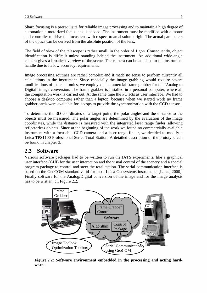
2.3 Software 9

Sharp focusing is a prerequisite for reliable image processing and to maintain a high degree of automation a motorized focus lens is needed. The instrument must be modified with a motor and controller to drive the focus lens with respect to an absolute origin. The actual parameters of the optics can be derived from the absolute position of the lens. The field of view of the telescope is rather small, in the order of 1 gon. Consequently, object identification is difficult unless standing behind the instrument. An additional wide-angle camera gives a broader overview of the scene. The camera can be attached to the instrument handle due to its low accuracy requirements. Image processing routines are rather complex and it made no sense to perform currently all calculations in the instrument. Since especially the image grabbing would require severe modifications of the electronics, we employed a commercial frame grabber for the ‘Analog to Digital’ image conversion. The frame grabber is installed in a personal computer, where all the computation work is carried out. At the same time the PC acts as user interface. We had to choose a desktop computer rather than a laptop, because when we started work no frame grabber cards were available for laptops to provide the synchronization with the CCD sensor. To determine the 3D coordinates of a target point, the polar angles and the distance to the objects must be measured. The polar angles are determined by the evaluation of the image coordinates, while the distance is measured with the integrated laser range finder, allowing reflectorless objects. Since at the beginning of the work we found no commercially available instrument with a focusable CCD camera and a laser range finder, we decided to modify a Leica TPS1100 Professional Series Total Station. A detailed description of the prototype can be found in chapter 3.

2.3 Software Various software packages had to be written to run the IATS experiments, like a graphical user interface (GUI) for the user interaction and the visual control of the scenery and a special program package to control and steer the total station. The serial communication interface is based on the GeoCOM standard valid for most Leica Geosystems instruments [Leica, 2000]. Finally software for the Analog/Digital conversion of the image and for the image analysis has to be written, cf. Figure 2.2.

Software

GUI CCDPC

FrameGrabber

ControlPackage

Serial Communicationusing GeoCOM

Frame GrabberControl

Algorithm

Image ToolboxOptimization Toolbox

Figure 2.2: Software environment embedded in the processing and acting hard-ware.

10 2 Concept for an image assisted total station

The software is mainly implemented in MATLAB, but time critical and hardware dependent parts like for the frame grabber are coded in C. MATLAB provides different toolboxes like these for image processing and for optimization, as well for GUI support, which helped to speed up the development. The PC environment for the software development is Win-dows 2000. It is not the aim of this project to develop software for real-time processing, but to demon-strate the feasibility of an image-assisted system. Therefore, the algorithms are not optimized with respect to processing speed.

3 Prototype Due to the unavailability of a total station with integrated camera, motorized focus lens and reflectorless distance measurement it is decided to build a prototype based on a Leica TPS1100 Professional Series instrument. [Uffenkamp, 1995] describes the concept and the experimental realization of an opto-electrical pan-tilt camera with long focal length. This camera is not based on a theodolite sys-tem, and it cannot measure distances. [Juretzko, 2001; Scherer, 2002] describe a theodolite system called TOTAL, which is equipped with an eyepiece camera that is primarily used for guidance and for profile scanning. Commercially available theodolites with CCD cameras are the Leica theodolite TM3000V and the Kern E2-SE. Newer models like the Leica TCA2003 use their camera to measure only the center of gravity of laser spots reflected by prisms for tracking and fine pointing purposes, which allows to employ a fixed focus optics. These instruments are therefore not suitable for an IATS. In this chapter we present the layout of the basic instrument, its hardware modifications in-cluding the implementation of the autofocus unit and comment on the stability of the CCD sensor.

3.1 Basic instrument Figure 3.1 shows the basic instrument we use, a Leica TCRM 1101 of the Leica TPS 1100 Professional Series [Leica, 2002].

Figure 3.1: Leica TCRM 1101.

This instrument is equipped with motorized horizontal and vertical drives. It also has a laser rangefinder (electronic distance meter EDM) to measure distances to prisms and to non-cooperative surfaces (Reflectorless EDM), which uses the phase measurement principle. The reflectorless EDM employs a visible red laser and is thus able to visibly mark the target with a bright spot, while the range finder to prisms uses an infrared laser. The specified distance ac-curacy for the infrared EDM is 2 mm + 2 ppm and for the red laser 3 mm + 2 ppm. The reflectorless EDM is well suited for measuring inaccessible objects, house corners, facades

12 3 Prototype

flectorless EDM is well suited for measuring inaccessible objects, house corners, facades and interiors.

3.2 Hardware modifications The total station is upgraded with a CCD camera, which produces an electronic image of a slightly smaller field of view as seen by a human operator through the eyepiece. Furthermore the focus lens is motorized, and a wide-angle camera for overview purposes is placed on top of the handle of the total station. Figure 3.2 a) shows a cross section of the telescope with the added parts. The CCD camera replacing the eyepiece and the reticle is covered by a protective cap. The cables for transmit-ting the video and the synchronization signals are fed through the hollow tilting axis. This minimizes the torque on the vertical axis that impedes vertical angle readings, cf. Figure 3.2 b). a)

Motor

Motor controller

Cable forimage transfer

Limitswitch CCD

camera

b)

Figure 3.2: a) Cross section of the telescope showing modifications. b) Prototype used in this thesis.

Both controllers for the focus motor and the CCD camera are placed on the upper side of the telescope, where the ATR (Automatic Target Recognition) hardware is normally located.

3.2.1 CCD camera and frame grabber The image registration is performed by a Sony camera module CCB-M35ACE [Sony, 1999] with the CCD image sensor ICX055BL for CCIR B/W video cameras [Sony, undated]. The eyepiece and the reticle are removed from the telescope, and the image sensor is placed in the image plane using a mechanical adapter with adjustments means to shift and rotate the image sensor. The table below shows the specification of the image sensor Horizontal Vertical Pixel size 9.8 µm 6.3 µm Number of pixels 488 572 Instantaneous field of view (IFOV) 2.7 mgon 1.8 mgon

Table 3.1: Specification of the Sony ICX055BL image sensor.

3.3 Autofocus 13

The camera control interface is a custom designed electronic board from Leica Geosystems, which allows adjusting the image integration time (Shutter) in 8 steps: Shutter 0 1 2 3 4 5 6 7 Integration time

0.1 ms 0.25 ms 0.5 ms 1 ms 2 ms 4 ms 8 ms 20 ms

Table 3.2: Integration time for the image sensor. Integration times are set by an instruction from the extended GeoCOM command set [Leica, 2000], the communication standard for Leica Total Stations. Some of the commands used in the current implementation are not for public use and provided from Leica Geosystems espe-cially for this work. Furthermore, the electronics delivers a permanent analog video stream, the horizontal and vertical sync signals and the pixel clock. To provide a stable image, a Ma-trox Meteor-II/Multi-Channel frame grabber [Matrox, 2001] is employed. The synchroniza-tion signals supplied by the image sensor accomplish the synchronization between camera and frame grabber [Matrox, 1996].

3.2.2 Focus drive The focus tube is moved by a Faulhaber DC-Micromotor 2224 U-SR with Encoder IE2–512, controlled by a MCDC 2805 Motion Controller from Faulhaber [Faulhaber, 2000]. The de-fault position of the focus lens is the infinity position marked by a limit switch. The communication is performed by GeoCOM commands.

3.2.3 Wide angle camera During the study we found as big advantage to attach as pointing help a wide-angle camera Sony XC-77CE on top of the handle of the theodolite; see Figure 3.3.

Figure 3.3: Prototype with wide-angle camera placed on top of the handle.

The Matrox Meteor-II/Multi-Channel digitizes the image. Since we need the image only for the coarse pointing, a synchronization of the frame grabber is not necessary. The field of view is about ±10 gon.

3.3 Autofocus Autofocus systems are known for many applications, where their most popular use is seen in consumer photography. Since the accuracy of image analysis methods depends on the infor-mation content in the image, a perfect focusing is needed, which must be automated. We can distinguish between focusing on known targets, as for example markers, and on non-

14 3 Prototype

signalized, unknown objects. The autofocus function of the IATS will be addressed only on the latter case, where no information of the object is available. [Kessler & Fischer, 2000] describe an analytic model of an autofocus system with CCD cam-eras and [Liao, 1993; Blessing, 2000] outline different possibilities of applying a contrast-based method for autofocussing. There exist different approaches of autofocus functions used in conjunction with the TM3000V video theodolite. [Roic, 1996] uses the moments of second order of statistics, namely the mean value and the standard deviation, to determine the image contrast. The maximum of the standard deviation normalized with the mean value delivers the best focus position. Unfortunately, this approach fails in situations, where we have extreme light condi-tions and depends highly on the structure of the aimed target, cf. [Mischke, 2000]. [Mischke, 1996; Mischke, 2000] developed this approach further. He proposes a contrast measurement based on the sum of the gradient between pixels in column and row direction, where the pix-els have a predefined distance. The number of registered gray-value changes is used to nor-malize. Only pixels above a certain threshold are taken into account for calculating the sums to eliminate the influence of scintillations. To determine the best focus position, he proposes a coarse search to roughly find the contrast maximum followed by a fine search in this region. The contrast values of the fine search are used to fit of a polynomial of third order, which de-livers the best focus position. He further indicates that his approach utilize the small field of view of the TM3000V. [Seatovic, 2000] proposes two new approaches. He uses the Fourier Transform to detect high frequencies in the image, which have to be maximized. The second one is to fit a straight line into the image of a known target line. The standard deviation of this fit increases for higher degree of defocus. To find the best autofocus function for the IATS we have to consider, that the optics systems of the TM3000V and the TPS1100 Professional Series theodolites differ significantly. The TM3000V employs a panfocal optics where the optical magnification is not linear in terms of the focused distance, while the TPS1100 optics design is analactic. The object area projected onto the CCD sensor differs significantly, while at 10 m an area of 30 ×20 mm2 is projected on the sensor in the TM3000V [Mischke & Wieser, 1995], the image sensor of the IATS cap-ture an area of 226 ×170 mm2. As a consequence of this, the IATS has to deal with more dis-turbances and objects at different distances within the measurement field of view. Taking all these differences into account, we cannot simply use the autofocus algorithms proposed above. The focusing procedure for the IATS is based either on the maximization of the image con-trast or using the information about the object distance measured by a range finder or on a combination of both. The disadvantage of the use of the range finder is the need to point the theodolite on the object so that the laser of the reflectorless EDM hits the target to be focused. In the following section we will outline different autofocus principles, active and passive sys-tems, and then describe in more detail the contrast based method to be used in the IATS. There, different contrast measurements are listed and a contrast measure based on Sobel filter-ing the image and measuring the pixel noise is derived. Further we will derive a mathematical description of the contrast function in terms of the blur width, which is a function of the focus lens position. Thus, the position where the blur is minimal describes the best focus position. Additionally, we describe an iterative method to determine the best focus position. Finally, we conclude this section by defining the autofocus method to be used with an IATS.

3.3 Autofocus 15

3.3.1 Autofocus principles An autofocus system should move the motorized focus lens to the position, which results in best image quality on the sensor.

3.3.1.1 Passive systems [Burkhardt, 1999] describes focusing systems based on triangulation procedures. a) b)

Figure 3.4: a) Basic setup for triangulation. b) Stereo setup with two cameras.

Figure 3.4 a) shows the principle of triangulation. From the following formulas the object distance p can be calculated as a function of the base b and the observation angles α1 and α2. ( ) ( )

( ) ( )21

21tantantantan

αααα

+⋅

⋅= bp (3.1)

where ( )

( )

21

22

11

tan

tan

bbbbp

bp

+=

=

=

α

α

This is equivalent to the human depth viewing to estimate distances. Such systems are called ‘passive’ because they employ two sensors but no actuators. If, however, one of the sensors is replaced by a light emitter like a laser diode, we speak of an ‘active’ system. In Figure 3.4 b) a setup with two image sensors in a stereo arrangement is shown. Using the theorem of intersecting lines we get:

21 ddqbp+

⋅= (3.2)

d1 and d2 are the deviations of the image position from a defined origin. Usually these two deviations are calculated by correlation methods. There are a large variety of triangulation systems. Figure 3.5 shows the one described in [EPSIC, undated]. It uses one image sensor and two mirrors. The mirrors are either fix mounted or can be angular adjusted. In the first case the offset between the images of the ob-ject relative to a calibrated center is used to compute the distance. In the second case the im-age of the object is moved to a central position by changing the angle of the mirror, from which the distance is estimated.

16 3 Prototype

Figure 3.5: Stereo system using mirrors and one sensor.

Figure 3.6 shows the setup of commercial autofocus cameras. Here it is possible to generate stereo images through a monocular objective. The diameter of the objective defines the dis-tance between the two single images on the detector row.

OP: Object plane PL: Photographic lens DP: Detector plane FL: Field lens AFR: Autofocus detector row SV: Signal voltage

Figure 3.6 Typical stereo setup for commercial cameras (Rollei). The basic principle is as follows: The light rays emerging from a point in the object plane pass through the upper and lower half of the photographic lens. Exactly at the position of the detector plane, there is a prism or a field lens. If the camera is correctly focused, then the rays pass through the center of the lens without refraction and are imaged on the two autofocus detector rows. If the camera is not correctly focused, then the rays are diverted either to the middle or to the outside of the detector. The image of the object point corresponds to the sig-nal voltage, which is laterally shifted, and low pass filtered due to the defocus. The lateral shift depends directly on the defocus. This principle is also known as Visiotronic, Correfot, Comparison of Phase-Contrast or Correlation Contrast. Figure 3.7 depicts the principle described above. The diagram is taken from the US patent 6 124 924. The optics contains a slit aperture, which generates an image in the fo-cal plane and two spatially separated images out of focus.

3.3 Autofocus 17

Figure 3.7: Optic schematic / US patent 6 124 924.

Another possibility for control the autofocus motion is the maximization of the image contrast on the sensor. These solutions are pure algorithmic, thus require no additional hardware and are the preferred choice for IATS. We describe them in detail in section 3.3.2.

3.3.1.2 Active systems Some active autofocus systems also use triangulation; as emitters one takes infrared diodes, laser diodes or ultrasound sources to measure the object distance or to produce a intensity spot on the sensor.

w

∆x

ProjectingLens

InfraredDiode

CCD

dObject

c

Figure 3.8: Active autofocus: Distance measurement by triangulation. The spot of an infrared LED is reflected from the object producing a spot on the CCD sensor. The spot offset from the sensor center is proportional to the object distance.

Figure 3.8 shows a system with an infrared LED to generate a spot on a sensor array, cf. [EPSIC, undated]. The emitted light is reflected from the target and imaged on a CCD, which is at a distance c from the lens. The distance w between the center of the emitter diode and the center of the CCD sensor is known by construction. From the spot offset ∆x on the sensor, the distance d can be calculated.

wxcd ∆

⋅= (3.3)

When measuring the distance to the object as control parameter for the autofocus several technologies exist today: The time of flight of a light pulse or the phase deviation for ampli-tude modulated light rays. In the US patent US 5 923 468 we find a focusing method based on the distance measurement of a range finder.

3.3.2 Contrast based autofocus Although passive autofocus systems require more computing efforts than active systems, they are often used in video cameras [Blessing, 2000].

18 3 Prototype

3.3.2.1 Contrast measure methods [Liao, 1993] describes eight methods for measuring the image contrast and [Blessing, 2000] extends those methods, which will be presented now. We will use the following definitions in describing contrast measures: g(x,y) Image L Number of columns of g R Number of rows of g M Number of pixels Variance of the gray level

( )[ ]

( )∑ ∑

∑ ∑−

=

−

=

−

=

−

=

−=

−=

1

0

1

0

22

1

0

1

0

2

,1

,1

L

x

R

yg

L

x

R

yg

myxgM

myxgM

VAR

(3.4)

where VAR Variance of the gray level to use as focus criteria mg Mean gray value of the image

Entropy of the gray level

( )∑=

⋅−=n

ggg ppENT

12log (3.5)

where ENT Entropy of the gray level to use as focus criteria pg Probability of the occurrence of the gray level g in the image n Number of gray levels

Sum modulus difference (SMD) Measure for the absolute gradient of the image. ( )∑ ∑

−

=

−

= ∂∂

=1

0

1

01

,1 L

x

R

y xyxg

MSMD (3.6)

( )∑ ∑−

=

−

= ∂∂

=1

0

1

02

,1 L

x

R

y yyxg

MSMD (3.7)

( ) ( )∑ ∑

−

=

−

=

∂

∂+

∂∂

=1

0

1

0

22

3,,1 L

x

R

y yyxg

xyxg

MSMD (3.8)

where SMD1 Sum modulus difference in x direction SMD2 Sum modulus difference in y direction SMD3 Combination of SMD1 and SMD2 to form a focus criteria

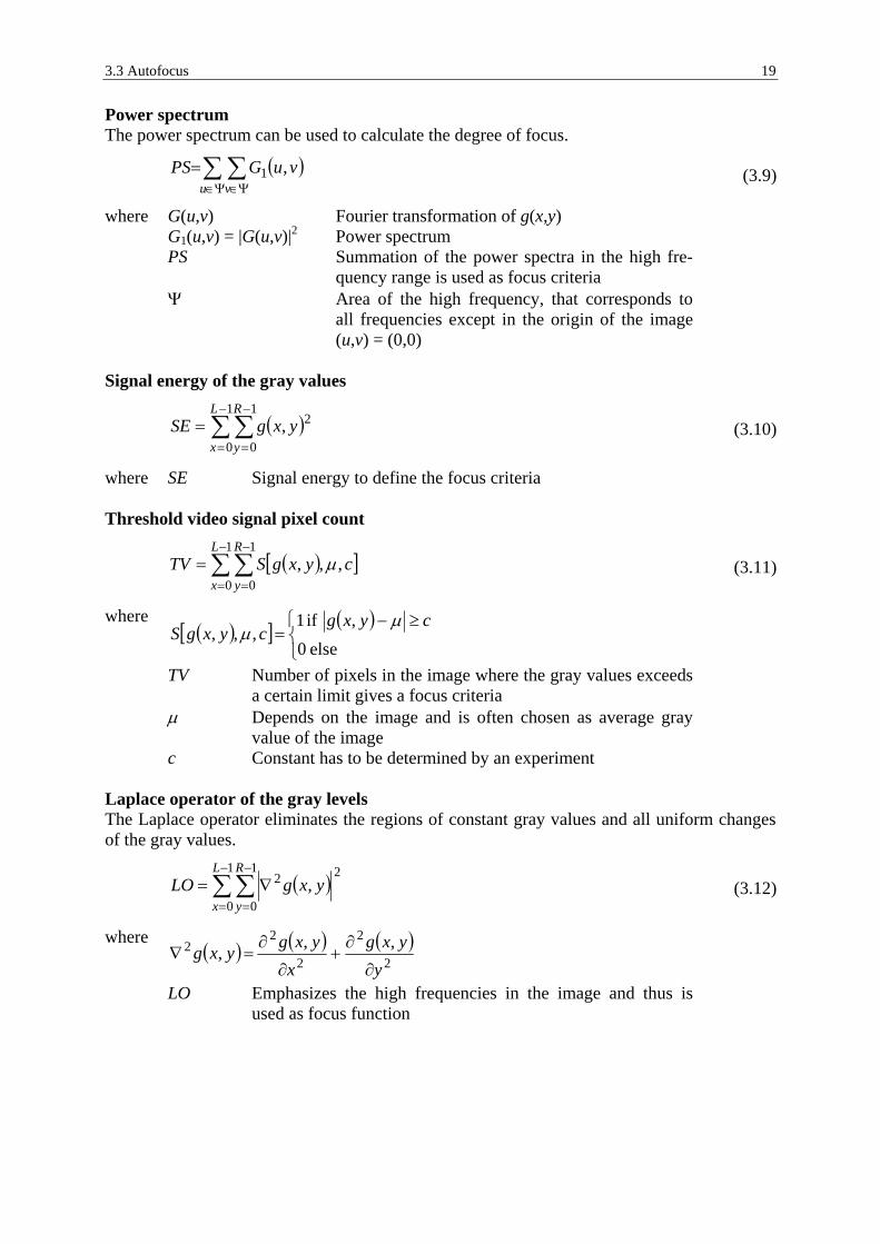
3.3 Autofocus 19

Power spectrum The power spectrum can be used to calculate the degree of focus. ( )∑ ∑

Ψ∈ Ψ∈=

u vvuGPS ,1 (3.9)

where G(u,v) Fourier transformation of g(x,y) G1(u,v) = |G(u,v)|2 Power spectrum PS Summation of the power spectra in the high fre-

quency range is used as focus criteria Ψ Area of the high frequency, that corresponds to

all frequencies except in the origin of the image (u,v) = (0,0)

Signal energy of the gray values

( )∑ ∑−

=

−

==

1

0

1

0

2,L

x

R

yyxgSE (3.10)

where SE Signal energy to define the focus criteria Threshold video signal pixel count

( )[ ]∑ ∑−

=

−

==

1

0

1

0,,,

L

x

R

ycyxgSTV µ (3.11)

where ( )[ ] ( )

≥−

=else0

, if1,,,

cyxgcyxgS

µµ

TV Number of pixels in the image where the gray values exceeds a certain limit gives a focus criteria

µ Depends on the image and is often chosen as average gray value of the image

c Constant has to be determined by an experiment Laplace operator of the gray levels The Laplace operator eliminates the regions of constant gray values and all uniform changes of the gray values.

( )∑ ∑−

=

−

=∇=

1

0

1

0

22 ,L

x

R

yyxgLO (3.12)

where ( ) ( ) ( )

2

2

2

22 ,,,

yyxg

xyxgyxg

∂

∂+

∂

∂=∇

LO Emphasizes the high frequencies in the image and thus is used as focus function

20 3 Prototype

Derivative of the variance The variance (VAR) of the gray values as function of the focus position p′ has a unimodal behavior in the area of the best focus. Therefore this function has its maximum (p′ part of the best focus area) when ( ) 0)( =′=

′∂′∂ pDVAR

ppVAR (3.13)

where VAR Variance of the gray levels To solve the influence of the noise, a low pass filter is used: ( ) ( ) ( )1−′⋅+′⋅=′′ pDVARbpDVARapRDVA (3.14)

where ( ) ( ) ( )1−′−′≈′ pVARpVARpDVAR a, b Constants satisfying a + b = 1

Square plane sum modulus difference (SPSMD) The approach of the SMD algorithm from [Liao, 1993] is extended to the SPSMD algorithm. The equations are

( ) ( )( )∑ ∑−

=

−

=−−=

1

0

1

0

2,1,L

x

R

yx yxgyxgSSMD (3.15)

( ) ( )( )∑ ∑

−

=

−

=−−=

1

0

1

0

21,,L

x

R

yy yxgyxgSSMD (3.16)

yx SSMDSSMDSPSMD += (3.17)

Factors affecting contrast measurement Contrast measurements include the calculation of either • the variance of the gray level, • the entropy of the gray level or • the Laplace operator of the gray level, which depend on the pixel brightness, but ignore their spatial distribution. This produces un-desired effects if parts of the images are over-saturated or perfectly dark. The maximum value of the variance occurs if half of the pixels are perfectly dark and the other half of the pixels are over-saturated. So if for example a small over-saturated spot happens to be in the field of view, contrast measurements tend to defocus the spot to get more pixels over-saturated. The defocus results in a bigger spot and thus produces a higher contrast value, because more pix-els of high gray level change are involved in the calculation.

3.3.2.2 Modified Sobel filter for contrast measure As mentioned in the previous section, many methods for contrast measurements are in use. A common problem is their susceptibility to noise. We developed a ‘robust’ contrast measure-ment method with reduced sensitivity to noise. It is based on a Sobel filter that is a variant of a gradient filter combined with a smoothing function. The averaging or smoothing part of the filter performs a spatial frequency low-pass filtering, which reduces noise at the cost of re-duced spatial resolution.

3.3 Autofocus 21

Sobel filter kernel for horizontal and vertical edge filtering:

−−−=

121000121

xS ,

−−−

=101202101

yS (3.18)

The following pseudo code gives an impression how this contrast functions works. • Take two consecutive images at the same focus lens position. Ensure that the discrepancy

between the two images is mainly due to noise. • Calculate the image difference (Subtract corresponding gray values)

( ) ( ) ( )yxgyxgyxg D ,,, 21 −= • Apply a Sobel filter in both directions and calculating the squared sum yields the Noise-

Level:

( ) ( ) ( )( ) ( )( )∑ ∑−

=

−

=+∗

−⋅−=

2

1

2

1

22 ,*,22

1 L

x

R

yDyDx yxgSyxgS

RLNoiseLevel

• We assume that image details to be taken into account have a higher contrast than the NoiseLimit i.e. the NoiseLevel multiplied by some integer factor. A value between 5 and 10 is optimal for this application.

• Apply the Sobel filter in both directions to one of the two images. If calculation time per-mits, the average of the two images can be used instead of either one. Calculate the squared sum of all pixels and add up all pixels, which are above the NoiseLimit.

( ) ( )( ) ( )( )212

1 ,*,*, yxgSyxgSyxh yx +=

( ) ( ) ( )∑−−

>==−⋅−

=2,2

1,1,

221 RL

NoiseLimithyx

yxhRL

Contrast

There are many ways to apply the contrast measure method. It is not necessary to calculate the contrast based on the whole image; for most application it is sufficient to apply it to the cen-tral part. Another approach could be to apply it to different sub-images or to implement sub-sampling in the calculation of the filter convolution.

3.3.2.3 Mathematical background of contrast measurement As already mentioned, the contrast calculation is based on a gradient calculation. In this sec-tion the mathematical background of this approach will be explained. The considerations are made for a 1D step edge and can be expanded to the 2-dimensional case. The contrast drops with increasing blur, means defocus. The blur can be modeled with a Gaussian or a square function. For our purpose, the approximation with a square function is sufficient. Instead of using the 2-dimensional Sobel filter, we will use the first derivative, which fulfills the considerations in 1D. Therefore we get the following definitions:

22 3 Prototype

Step edge function: e(x,a) x: Spatial position a: Edge width Blur function: b(x,σ) x: Spatial position σ: Blur width

Figure 3.9: Step edge and blur definition.

The blur width σ is calculated based on the circle of confusion (COC). The COC depends on the best focus position and the actual focus position. In Figure 3.10 the geometrical meaning of the COC is outlined.

Image PlaneObject

Focus LensMain Lens

Focus Error

Circle ofConfusion

Figure 3.10: Definition of the circle of confusion.

The calculations concerning the COC for the prototype are based on TPS1100 Series optics. The contrast depends on the slope of the edge and of the size of the blur as defined above. It results in the following formula

( ) ( ) ( )( )∫∞

∞−

= dxxbaxe

dxdaC

2,*,, σσ (3.19)

The result for the contrast function in terms of a discrete sampling amounts to

( )( )2

2

131

11,

+

−−

+=

σσσ

aaaC , for 1+≤ σa (3.20)

( ) ( )

( )1321, 2 +

+−=

σσσσ

aaaC , for 1+< σa (3.21)

3.3 Autofocus 23

The underlying contrast function used in the autofocus algorithm can now be defined by:

( ) 421

341 1, p

ppppC +

+−⋅=

σσK (3.22)

where p1 Peak width p2 Location of the peak maximum p3 Scaling p4 Bias

All four parameters could be used for validity checks. It is possible to determine these pa-rameters by a least squares fit using sampled contrast data at different focus lens positions.

3.3.2.4 Optimization for maximization of contrast Contrast based autofocus means maximizing the image contrast as a function of the focus lens position. There are some obstacles that complicate this task. Firstly, off-the-shelf optimization algorithms, e.g. Golden Section Search, tend to overly large variations of the optimization parameter (focus lens position) in successive iterations. This leads to excessive lens movements and unacceptable processing times. Accordingly, an opti-mization algorithm is needed that operates more local. A second problem poses the noise in the images; it impedes contrast calculations. This prob-lem is adequately dealt with organizing the optimization in such away that only significant changes of contrast are taken into account. Finally, the depth-of-field of the Leica theodolite optics is rather poor. This is a consequence of the lens system designed to operate under severe light conditions. All this amounts to small contrast changes if the object in sight is strongly defocused. In order to improve this situation we derived a new algorithm. a)

0 1 2 3 4 5Lens Position

Con

trast

0.2

0

0.4

0.60.8

1.0

b)

0 1 2 3 4 5Lens Position

Con

trast

0.2

0

0.4

0.60.8

1.0

c)

0 1 2 3 4 5Lens Position

Con

trast

0.2

0

0.4

0.60.8

1.0

Figure 3.11: Finding the maximum contrast position. a) First contrast measure-ment. b) Adding a second contrast measurement. c) Adding a third contrast meas-urement.

In order to get an initial estimate of the NoiseLevel, the autofocus process starts with several evaluations of the contrast function at a constant focus lens position. In Figure 3.11 and Figure 3.12 the contrast for a single object in the field of view is drawn as a function of the focus lens position. The contrast function is evaluated at the current focus lens position; de-picted by a circle in Figure 3.11 a). Then the focus lens is moved towards focus position infin-ity; the step size has a prescribed value or is chosen as a function of the current focus lens position.

24 3 Prototype

After the first lens position step the contrast is determined again (Figure 3.11 b), diamond). The algorithm continues stepping in the same direction until the change of contrast compared to the first try is significant (a certain factor higher than the Noise Level). From then on the direction of search is clear, and the algorithm continues stepping towards higher contrast in the same direction (Figure 3.11 c), cross) while it always keeps the two previous positions (Figure 3.11 c) circle and diamond). In that way it “climbs up the hill” (Figure 3.12 a))... a)

0 1 2 3 4 5Lens Position

Con

trast

0.2

0

0.4

0.60.8

1.0

b)

0 1 2 3 4 5Lens Position

Con

trast

0.2

0

0.4

0.60.8

1.0

c)

0 1 2 3 4 5Lens Position

Con

trast

0.2

0

0.4

0.60.8

1.0

d)

0 1 2 3 4 5Lens Position

Con

trast

0.2

0

0.4

0.60.8

1.0

Figure 3.12: “Hill climbing strategy” for determine the maximum contrast posi-tion. a) Climb up the hill. b) Passing the maximum position. c) Refining the maxi-mum peak. d) Final measurement situation.

… until it passes the optimal position (Figure 3.12 b)). The lens moves on until the current image (cross) has significantly lower contrast than the preceding one (diamond). From that point on the lens moves backwards and forward in a plausible way until it converges to a local contrast maximum (Figure 3.12 c) and d)). This procedure has been tested extensively and it turned out to be stable even in volatile environments.

3.3.3 Implemented algorithm Our measurement equipment is well suited for two different autofocus systems. The obvious choice is the use of the laser range finder to get the best focus position. A disadvantage of this approach is that the ranger must point at the object to be focused on. The second choice is maximization of the contrast as described above. Contrast calculations are performed in a pre-assigned image region. If the initial image is totally defocused, search time can get long since the whole focus range must be inspected. As an alternative to the it-erative maximization of the contrast, contrasts can be evaluated at discrete positions and then the contrast function (3.22) is used in a fitting yielding the maximum position. Clearly, the two approaches can be combined: Use the ranger to roughly position the focus lens, and then start contrast maximization.

3.4 Stability tests 25

Manufacturers of surveying instruments already offer autofocus functionality in some of their instruments: Topcon Digital Level DL-103AF with autofocus is available. Pentax: Digital Levels AFL-240, AFL-280, and AFL-320, and Total Station R-100 Series

with autofocus. The autofocus uses a phase contrast method, the method also used for photo cameras.

3.4 Stability tests Adding new measurement devices like the CCD, the limit switch and the motorization of the focus lens should keep the specified stability of a total station. The stability tests we per-formed are presented in this section.

3.4.1 CCD switch-on drift The aim of this test is to find out if there is any unacceptable mechanical drift of the CCD sensor during the system’s warm-up. We check this by measuring an eventual image drift of a stationary object. As test set up we take a high precision electro-optical collimator (EO) with built in laser pointer and receiver.

Figure 3.13: Setup for measuring the CCD switch-on drift.

The theodolite and the EO are mounted on a granite plate (Figure 3.13). A mirror reflecting 50% of the incident laser light is placed on the front side of the telescope. The laser beam is simultaneously recorded on the CCD of the theodolite and on the collimator detector. Since the laser is modulated at 4 kHz, at least 10 images are averaged for one spot measurement. Additionally, the theodolite angles and the tilt angles are recorded during the measurement. To determine the dependence between the position measurements of the theodolite and the EO-collimator, we need a calibration first of viewing angle versus spot position on the sensor. We do this by measuring the spot position ∆x as function of different theodolite angles. The exact dependence is found by applying a least squares matching algorithm. The measurement principle is described in chapter 5. Furthermore, the measured values of the EO-collimator ∆EO are recorded. Knowing the angular movement of the theodolite, the relationship between pixel shift ∆x, respectively between EO-collimator readings ∆EO and theodolite angles can be derived.

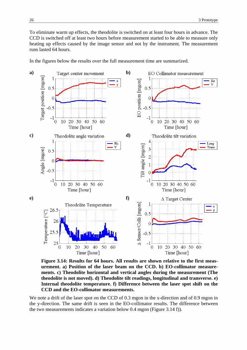
26 3 Prototype

To eliminate warm up effects, the theodolite is switched on at least four hours in advance. The CCD is switched off at least two hours before measurement started to be able to measure only heating up effects caused by the image sensor and not by the instrument. The measurement runs lasted 64 hours. In the figures below the results over the full measurement time are summarized. a) b)

c) d)

e) f)

Figure 3.14: Results for 64 hours. All results are shown relative to the first meas-urement. a) Position of the laser beam on the CCD. b) EO-collimator measure-ments. c) Theodolite horizontal and vertical angles during the measurement (The theodolite is not moved). d) Theodolite tilt readings, longitudinal and transverse. e) Internal theodolite temperature. f) Difference between the laser spot shift on the CCD and the EO-collimator measurements.

We note a drift of the laser spot on the CCD of 0.3 mgon in the x-direction and of 0.9 mgon in the y-direction. The same drift is seen in the EO-collimator results. The difference between the two measurements indicates a variation below 0.4 mgon (Figure 3.14 f)).

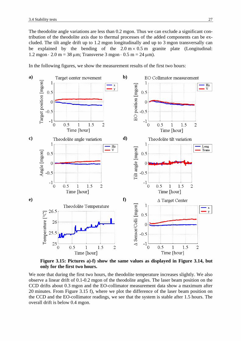
3.4 Stability tests 27

The theodolite angle variations are less than 0.2 mgon. Thus we can exclude a significant con-tribution of the theodolite axis due to thermal processes of the added components can be ex-cluded. The tilt angle drift up to 1.2 mgon longitudinally and up to 3 mgon transversally can be explained by the bending of the 2.0 m × 0.5 m granite plate (Longitudinal: 1.2 mgon ⋅ 2.0 m = 38 µm; Transverse 3 mgon ⋅ 0.5 m = 24 µm). In the following figures, we show the measurement results of the first two hours: a) b)

c) d)

e) f)

Figure 3.15: Pictures a)-f) show the same values as displayed in Figure 3.14, but only for the first two hours.

We note that during the first two hours, the theodolite temperature increases slightly. We also observe a linear drift of 0.1-0.2 mgon of the theodolite angles. The laser beam position on the CCD drifts about 0.3 mgon and the EO-collimator measurement data show a maximum after 20 minutes. From Figure 3.15 f), where we plot the difference of the laser beam position on the CCD and the EO-collimator readings, we see that the system is stable after 1.5 hours. The overall drift is below 0.4 mgon.

28 3 Prototype

Two measurement series were performed to determine the temperature drift of the CCD inde-pendent of any uncontrolled theodolite motion. Both series show a small drift of the CCD below 0.4 mgon during the first hour after switch-on. In most applications, a drift of below 0.4 mgon is acceptable and no ‘warm up’ time is needed between instrument switch-on and start of the measurement. In applications of high accuracy the theodolite and the CCD sensors should be switched on at least one hour before the measurement start to avoid thermal insta-bilities. Because this is a significant limitation in practice, the thermal drift should be elimi-nated. This could be realized by applying an additional temperature sensor near the CCD and by calibrating the drift in terms of temperature and time. But this will be a task of the product development.

3.4.2 Focus lens positioning From the position of the focus lens along the optical axis we get the optical parameters needed for the algorithms. We will test the lens positioning accuracy by driving the focus lens for-ward and backward. The focus lens is first moved in positive direction and every 25 steps the contrast is calculated using the contrast based autofocus algorithm, cf. section 3.3.2. After passing the best focus position we repeat the procedure but now moving the lens in the negative direction. Both measurements are performed twice. As object we placed a target picture at a distance of ap-proximately 3 m.

Figure 3.16: Contrast values relative to the focus lens encoder position when mov-ing the focus lens in both directions.

Figure 3.16 shows the normalized contrast for positive and negative positioning. There is a significant difference in the maximum contrast position. Table 3.3 shows that both series lead to the same result and the difference of the maximum positions is approximately 90 steps, which corresponds to roughly 90 µm. Series I [steps] Series II [steps] Maximum positive search -8765 -8765Maximum negative search -8853 -8852Maximum difference 88 87

Table 3.3: Best focus position for positive and negative lens moving.

We conclude that the positioning of the focus lens must always be executed in the same direc-tion, especially to determine the zero position defined by the limit switch. Because the zero

3.4 Stability tests 29

positioning is found when moving the lens in positive direction, all further positioning must also be done in the positive direction. The positioning algorithm allows only positive position-ing motions.

3.4.3 Limit switch accuracy The accuracy of the absolute focus lens position is essential to the achievable accuracy of the system. The focal length directly depends on the focus lens position, which is coupled to the focus motor, explained in section 4.1. Here, the accuracy of the focus lens positioning in con-junction with the limit switch is examined. The position where the limit switch changes from “closed” to “open” or vice versa defines the origin of the motor encoder of the focus lens. This position should be very stable to provide a constant origin during lifetime of the instru-ment or until a new calibration is necessary. A shift of the origin influences directly the posi-tion of the focus lens relative to the front lens derived from the motor encoder measurements. The influence of the limit switch to the positioning accuracy of the focus lens is determined separately in two check runs. First a repeatability test of the position where the limit switch changes its state, and secondly a long duration test, where the theodolite and the motion con-troller are switched off between the measurements, are employed.

3.4.3.1 Repeatability after initialization The procedure for checking the repeatability of the limit switch is as follows: 1. The motion controller is initialized and the speed of the initial zero positioning selected. 2. The speed of the different positioning sequences is set (it differs from the initial speed). 3. Set zero position of the limit switch using the initial speed and moving in positive direc-

tion. 4. Set the edge trigger of the limit switch for the motion controller. 5. Start measurement series for each positioning speed

a) Motor is moved to the start position, either on the positive or the negative side of the zero position. The distance to the zero position is 1000 steps.

b) Set triggers of the motion controller to stop when the limit switch changes its state [Faulhaber, 2000]

c) Start positioning towards zero position d) After stopping the position is saved e) Repeat until the number of measurements is reached

6. Reset the speed of the motion controller 7. Terminate measurement This procedure is applied using the initial speeds 10, 30, 60 and 120 rpm. Then the position where the limit switch changes its state is evaluated using the speeds 10, 30, 60 and 120 rpm. In Figure 3.17 the results for initial speed of 60 rpm is shown. Not surprisingly, the reposi-tioning using 60 rpm yields the best results. Therefore, it is recommended to use 60 rpm for all positioning. The positioning direction influences the result drastically. The difference be-tween positive and negative direction is about 440 steps as can be seen in the right image showing the average position found in the test. Therefore positioning should take place al-ways in the same direction, as already stated in the previous section.

30 3 Prototype

Figure 3.17: Offset of the limit switch zero position for an initial speed of 60 rpm compared with different moving speeds during operation.

3.4.3.2 Long term repeatability In addition to the testing of different speeds used for setting the zero position, the long-term stability of the zero position has to be inspected. If the zero position drifts with time, then an adequate compensation must be found to calculate the absolute position. The long-term repeatability test is defined as: 1. The motion controller is initialized. The speed of setting of the zero position is set to

60 rpm according to the results of the previous test. 2. Speed for all positioning is set to 60 rpm 3. Set the limit switch trigger to indicate a change of its state 4. Start series

a. Record time b. Start zero positioning. Iteratively position towards the limit switch 40 times and save

the positions. This procedure is equal to the loop of the previous test c. Go to zero position d. Switch off theodolite and motion controller e. Wait 30 minutes f. Switch theodolite on g. Enable motion controller (Focus lens is still at zero position) h. Go back to a) until all series are executed.

5. Save all positions 6. Terminate procedure This procedure yields the position where the limit switch changes its state over time relative to an initial zero setting. Figure 3.18 shows the average position and the standard deviation of each series. The average position has a range of up to 12 steps, while the standard deviation is small compared to it. This fact must be taken into consideration when calculating the optics configuration based on the focus lens position.

3.4 Stability tests 31

Figure 3.18: Average and standard deviation for setting the zero position of the limit switch relative to an initial zero position using speed 60 rpm.

4 Modeling Typical features of a theodolite and a small angle photogrammetric camera are combined in a video theodolite, and thus holds for the IATS. The horizontal and vertical circles and the fo-cus drives are motorized and electronically readable. For an object point observation, the theodolite must be positioned, that the image of the object point is visible in the image. Using image processing algorithms the point coordinates in the image are determined. The distances relative to the principal point, the intersection point of the optical axis with the image sensor, together with the inner orientation yields the polar angles in direction to the tilting and stand-ing axis, respectively. By adding the theodolite angles (outer orientation), the final observa-tions are derived [Deumlich & Staiger, 2002]. [Wester-Ebbinghaus, 1985] describes the combination of a photogrammetric camera system with a terrestrial geodetic measurement system and extends the approach of the central projec-tion. [Huep, 1988] shows how the pointing directions of the theodolite are to be corrected by image coordinates to derive the horizontal and vertical angles of an object. This calculations are made with respect to the video theodolite TM3000V, which has a field of view about ten times smaller the IATS prototype. As a result of this, it is not necessary to consider, that the vertical pointing direction of pixels on a horizontal CCD line differ if the theodolite vertical angle is different from horizontal. Further, the TM3000V employs a reference frame to derive the inner orientation and to compensate thermic effects. [Uffenkamp, 1995] proposes an opto-electronic tilting-turing-camera and outlines the imaging model. For focusing purpose he moves the image sensor and the use of a reseau plate enables to provide constant transformation geometry. However, this optics concept is completely dif-ferent from that of the IATS. The system modeling for the TM3000V and the tilting-turning-camera are highly focused on the corresponding optics and mechanics, which differ significantly from those of the IATS. Further, that the IATS has not reseau plate or reference frame to determine the inner orienta-tion and the optical concept and the focusing mechanism are also different. According to all those differences we are forced to reconsider the modeling of the object point transformation from the sensor plane into the object space. In following sections we describe the relation between the optical and the mechanical parame-ters and derive effects on the image caused by those parts. The complex optics relations are simplified to a pinhole model and the influence of defocusing is examined. Further the theodolite axis errors are outlined and considered in the development of the mapping function from sensor plane into 3D object space. The chapter is concluded with an analysis of the sys-tem accuracy in terms of the single sensors.

4.1 Optics and mechanics The imaging relation from the object plane to the sensor array depends on the actual optical parameters, which are altered when moving the focusing opto-mechanical subsystem. We will derive the geometrical transformation from the 3D object space to the 2D image plane and consequently its inverse, which we need to reconstruct the object coordinates back from the measurement data.

34 4 Modeling

To get a better understanding we shortly line out how a optical system works: Any optical system must be understood as a ‘dual’ system, imaging the object field OBJ on its conjugate, the image field IMA on the sensor, but also images the entrance pupil ENP on the exit pupil EXP (Figure 4.1).

OBJ ENP EXPIMA

s's

Figure 4.1: Relation between the object and the image field.

The meaning of the entrance pupil is best understood by considering a single object field point. We assume that light from point OBJ is emitted into a broad angular cone and only some part of it is picked-up by the aperture YOBJ of the entrance pupil. The sinus of the col-lecting angle, as seen by the object point and defined as ratio of the ENP diameter YENP and the distance s between Obj and ENP, is called the numerical aperture NA. The product NA with YOBJ yields a quantity Inv = (YOBJ ⋅ YENP) / s, which might be in an analog way defined at the image side as Inv’ = (YIMA ⋅ YEXP) / s′. As can be seen by simple optical construction: Inv = Inv’, thus called the ‘invariant’. It describes the optical system in many aspects: First, when squared and multiplied with the object radiance πS*, one gets the amount of picked-up energy by the optics, which is com-pletely transferred to the sensor, assuming no absorption inside; i.e. Inv describes the conser-vation of energy. Another important property is the optical resolution: light is diffracted at the entrance aperture and shows an angular diffraction spectrum δω = m ⋅ 1.22 ⋅ λ / YENP, where m is the integer diffraction order and where we obtain the first intensity minima at m = ±1. Ignoring for the following the factor 1.22 and multiplying the angular spread δω by s results in an equivalent object resolution δy = s ⋅ δω ≈ λ / NA. Then the number of resolvable object points by the optics in both lateral dimensions is N = (YOBJ / δy)2 = (Inv / λ)2, the ratio of the system invari-ant Inv and the wavelength of light as information carrier. N is also called the space-bandwidth product, which clearly indicates that all optical systems can transfer only a limited amount of information. It is interesting to see that N depends on the amount of collected en-ergy, i.e. N couples both: energy and information (the fundamental first and second law of thermodynamics). Back to the object field: The light ray from an object point to the center of the entrance pupil, i.e. where the optical axis hits the ENP, is called the ‘chief ray’. In most cases this ray characterizes the center of gravity of the traveling light intensity everywhere in the system. Following this ray will allows us to describe e.g. defocusing effects, but also al-lows us to apply a ‘pinhole’ model for the reconstruction process. Both imaging processes, OBJ to IMA and ENP to EXP, have different magnifications, which depend however on each other:

ss

ss

YY

YY

PupilEXP

ENP

OBJ

IMAObj

′⋅=

′⋅==

ββ 1 (4.1)

4.1 Optics and mechanics 35

On the other hand, they are differently aberrated by distortions, which the lens designer has to control carefully.

4.1.1 System description The optical system of the theodolite telescope consists of two lenses, the objective, called the main lens, and the focusing lens. The beam splitter cubes for in and out coupling laser radia-tion, and the erecting prisms are irrelevant for our purposes and will be ignored, cf. Figure 4.2. For well-corrected optics and for small field angles, both being the case of our theodolite, we can describe the imaging properties in paraxial approximation.

MainLens

FocusLens

TiltingAxis

ImageSensor

OpticalAxis

Figure 4.2: Theodolite telescope with two lenses.

Figure 4.3 illustrates the optical system. The main lens and the image plane are fixed inside the body, while the focus lens is moved in z-direction, called the nominal optical axis. This axis should also be the mechanical pointing axis, defined as orthogonal axis to the tilt and standing axis of the theodolite. In case of lateral decentering errors of the focusing lens, the overall optical axis would show pointing errors and would no longer coincide with the me-chanical pointing axis. However, extreme careful mechanical construction and manufacturing assure that both axes coincide during refocusing even under severe environmental conditions. The origin of the optical system is placed in the front vertex of the main lens.

(+) dL1

(+) xO2

(+) xI1

(+) xI2

(+) xO1 (+) f12(+) f11

F11 F12

(-) h11 (-) h12

H12 H21 H22

(+) h21 (+) h22

(+) d

(-) f21

(-) f22

Object

ImagePlane

Tilting Axis

(+) doffset

Main Lens Focus Lens

(+) e

(+) dL21

(+) LS

(+) LSL

(+) dL2

(+) ∆H2

(+) sO1

(+) dO

ENP

rEP

(-) dENP

H11

F21F22

Figure 4.3: Optical parameter definition in terms of the mechanics.

36 4 Modeling

The table below describes the relevant optical parameters: f1 Focal length of the main lens (f1 = f11 = −f12). h11 Distance between the front principal plane and the front vertex of the main lens. h12 Distance between the back principal plane and the back vertex of the main lens. dL1 Thickness of the main lens f2 Focal length of the focus lens (f2 = f21 = −f22). h21 Distance between the front principal plane and the front vertex of the focus lens. h22 Distance between the back principal plane and the back vertex of the focus lens. dL2 Thickness of the focus lens ∆H2 Distance between the principal planes of the focus lens e Distance between the back principal plane of the front lens and the front principal

plane of the focus lens. LS Distance between the image sensor and the back principal plane of the main lens. dL21 Distance between the main and the focus lens measured from rear to front vertex. doffset Distance between the tilting axis and the front vertex of the main lens. dENP Distance between the entrance pupil and the front vertex of the main lens.

Table 4.1: Definition of the relevant optical parameters. In the following calculations, we will use the notation and the sign convention as defined in [Hecht, 2002]. sOj, fOj + Left of the front vertex of lens j xOj + Left of the front focal point Fj1 of lens j sIj, fIj + Right of the rear vertex of lens j xIj + Right of the rear focal point Fj2 of lens j yO, yI + Above the optical axis

Table 4.2: Sign convention for optical parameters. The optical parameters of both lenses and their intermediate distance define the optical sys-tem, which can be expressed by a joint focal length and two principal planes. The parameters of the total system are given by

effff

f−+

⋅=

21

21 (4.2)

11

21

111

21 h

efffeh

fefh +

−+⋅

=+⋅

= (4.3)

22

21

222

12 h

efffeh

fefh +

−+⋅

=+⋅

−= (4.4)

where f Focal length of combination of main and focus lens h1 Distance between the front principal plane H1 and the front vertex

of the combination of main and focus lens h2 Distance between the back principal plane H2 and the back vertex

of the combination of main and focus lens The following imaging equations are valid with respect to a fixed point of the theodolite, the front vertex of the main lens.

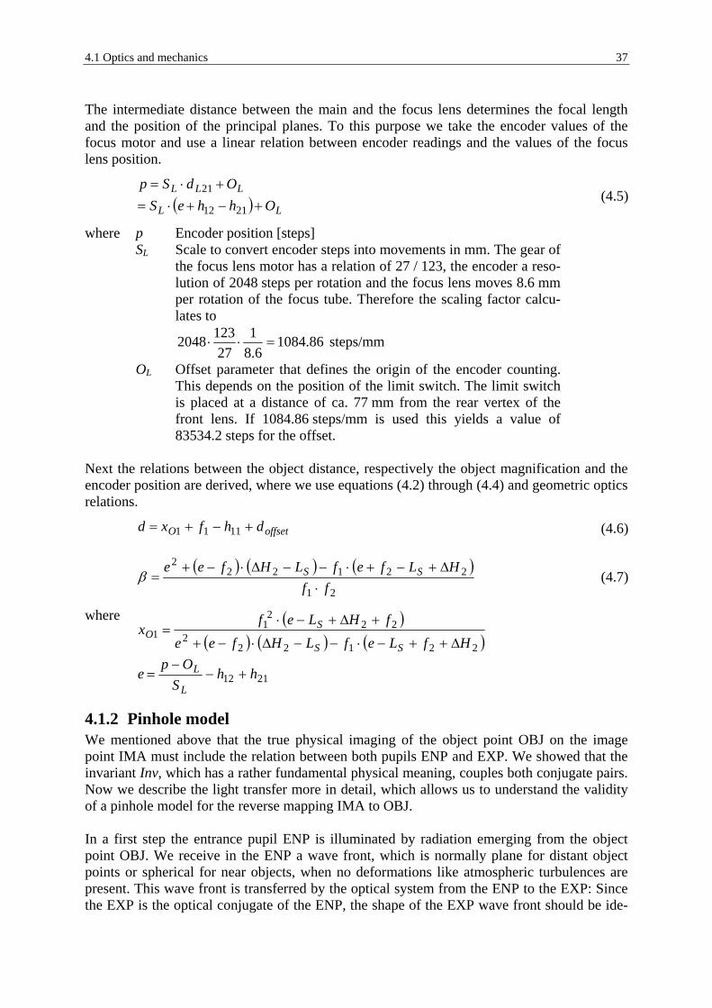
4.1 Optics and mechanics 37

The intermediate distance between the main and the focus lens determines the focal length and the position of the principal planes. To this purpose we take the encoder values of the focus motor and use a linear relation between encoder readings and the values of the focus lens position.

( ) LL

LLL

OhheSOdSp

+−+⋅=+⋅=

2112

21 (4.5)

where p Encoder position [steps] SL Scale to convert encoder steps into movements in mm. The gear of

the focus lens motor has a relation of 27 / 123, the encoder a reso-lution of 2048 steps per rotation and the focus lens moves 8.6 mm per rotation of the focus tube. Therefore the scaling factor calcu-lates to

steps/mm 86.10846.8

127

1232048 =⋅⋅

OL Offset parameter that defines the origin of the encoder counting. This depends on the position of the limit switch. The limit switch is placed at a distance of ca. 77 mm from the rear vertex of the front lens. If 1084.86 steps/mm is used this yields a value of 83534.2 steps for the offset.

Next the relations between the object distance, respectively the object magnification and the encoder position are derived, where we use equations (4.2) through (4.4) and geometric optics relations.

offsetO dhfxd +−+= 1111 (4.6)

( ) ( ) ( )21

221222

ffHLfefLHfee SS

⋅∆+−+⋅−−∆⋅−+

=β (4.7)

where ( )( ) ( ) ( )22122

222

21

1HfLefLHfee

fHLefx

SS

SO

∆++−⋅−−∆⋅−+

+∆+−⋅=

2112 hhS

Ope

L

L +−−

=

4.1.2 Pinhole model We mentioned above that the true physical imaging of the object point OBJ on the image point IMA must include the relation between both pupils ENP and EXP. We showed that the invariant Inv, which has a rather fundamental physical meaning, couples both conjugate pairs. Now we describe the light transfer more in detail, which allows us to understand the validity of a pinhole model for the reverse mapping IMA to OBJ. In a first step the entrance pupil ENP is illuminated by radiation emerging from the object point OBJ. We receive in the ENP a wave front, which is normally plane for distant object points or spherical for near objects, when no deformations like atmospheric turbulences are present. This wave front is transferred by the optical system from the ENP to the EXP: Since the EXP is the optical conjugate of the ENP, the shape of the EXP wave front should be ide-

38 4 Modeling

ally unaltered, eventually up or down scaled in its spatial extension dependant on the pupil magnification. However, we have to accept unavoidable wave front degradations: The first one we men-tioned is the light diffraction at the finite aperture of the ENP, which limits the spatial fre-quency content. Even if the wave front deviation from the plane is zero, the diffraction at the aperture boundary alone let each optical system act as ‘low pass’ information filter, which smears out fine details in the object wave front. The higher the NA, the better the resolution, but clearly also, the lower the wavelength, the better. The spatial resolution is further lowered by lens aberrations, but also by surface errors of the lenses or by mechanical mounting errors like lens decentering. Consequently, the wave front, which is reemitted by the exit pupil EXP to converge at point IMA, is more or less disturbed leading to a blurred image spot. In a best case situation the spot image of a single object point is the Airy function, well described in any optical handbook. Both propagations, the one from object OBJ to ENP, and the other EXP to image IMA are described by a 2D-Fourier transformation of the complex optical wave front, an approxima-tion of the diffraction mechanism, allowable for well-corrected systems. If the optical system is carefully designed, the intensity maximum of the diffracted spot is found in the image plane where the ‘chief ray’ hits the image plane. Thus we can replace the complex wave front propagation process by ray optics. Especially tracing the chief ray back from the image plane to the EXP, then to the ENP and from there in direction OBJ is a good approach for the desired back transformation. In conclusion, we work in the following with a simplified optical system where the light emit-ted from the object point as light cone and filling the aperture ENP is reduced to its chief ray, hitting the ENP on the optical axis. The interesting reverse process can be then thought that a pinhole, located at ENP, emits or receives only one light ray, the chief ray. But it must be clearly emphasized, that any kind of distortion introduced by the optical system like a wave front degradation, a geometrical distortion or even a vignetting must be identified in the ‘measurement space’ (EXP, IMA) and from there be transferred to the ‘object space’ (ENP, OBJ) for a correct reconstruction. There is finally another important property of the pupils: their position defines the perspective of the image. Modern digital photogrammetric cameras are telecentric at the image plane meaning that the exit pupil is located at infinity. There are several reasons for it: the most im-portant is to avoid color shading. Color filters, consisting of many dielectric thin layers, must be placed near to or at the sensor plane. To achieve the required sharp bandpass characteristic, all chief rays must be incident under the same angle, i.e. normal to the sensor plane. Other-wise pixel dependent color shifts occur, which are difficult to correct for color pictures, but are a true loss of information in case of remote sensing applications. There are more argu-ments favoring telecentric systems like the avoidance of ghost images and the insensitiveness to defocus. This is different in classical photogrammetric systems like the film cameras, [Kraus, 1997]. Here the pupils are at finite location and the optical mapping process is de-scribed by a central perspective transformation with the projection center in the entrance pupil ENP of the optical system.

4.1 Optics and mechanics 39

Then the mathematical image plane can be found in a distance c, called the camera constant. This plane, however, has to be known with respect to the instrument’s origin T0, which is de-fined as the intersection of the standing and tilting axis.

QENP EXP Image

PlaneMathematicalImagePlane

c

q

τ

τ'

yQ

yqsENP

Figure 4.4: Camera constant and projection center definition.

The angle τ of the incoming chief ray from Q is not equal to the angle τ′ of the outgoing chief ray. If we select the ENP as projection center, we must mathematically move the image plane to a new position yielding a mathematical image plane (MIP). The camera constant c is then defined as the distance between the ENP and the MIP. Further, we have the relation tan(τ) = yq / c. The camera constant can be expressed in terms of magnification and object distance or directly by the optics-mechanics parameters.

( ) ( )( )( )(( )( ))22111

222

11121

1

HLfehdf

LHfeedhfff

s

syy

c

SENP

SEP

ENP

ENPQ

q

∆+−++

+−∆−+−−⋅

=

⋅=

⋅=

K

β (4.8)

where sENP Distance between the entrance pupil and the object. This distance is measured along the optical axis.

β Magnification; defined by the focus lens position described by e dENP Distance between the entrance pupil and the front vertex of the

main lens (Figure 4.3). ∆H2 Distance between the principal planes of the focus lens

(Figure 4.3); ∆H2 = dL2 – h21 + h22 The camera constant increases with larger object distance and, by construction, with decreas-ing encoder position of the focus lens motor, respectively. Further, the changes per distance tend to zero for objects at farer distance as can be seen in Figure 4.5. The reason therefore is the fact, that the focal length and the image distance changes if the focal lens is moved. In photogrammetric cameras where the focal length is fixed, the camera constant decreases with larger distances.

40 4 Modeling

Figure 4.5: Camera constant in terms of object distance and encoder position of the focus motor.

As we will see in the next section, it is important to have the projection center in the theodolite origin, which makes the object polar angle calculation independent of the object distance. If the projection center does not coincide with the standing axis, the object dis-tance d must be known to get the object polar angle ϕ relative to the theodolite origin. The problem is illustrated in Figure 4.6.

ImageSensor

ENP

TO

Q

Pointing Axis

τ ϕd

c

yq

∆ENP

sENPq

Figure 4.6: Offset between projection center and theodolite origin.

The angle τ is defined by the camera constant c and the position q in the image. The angle ϕ is then calculated by

( ) ( ) qENPENP

ENP ycs

s⋅

⋅∆+=ϕtan (4.9)

If the offset between entrance pupil and theodolite origin goes to zero, the angle ϕ equals the angle τ.

4.1.3 Influence of defocusing We will measure the polar angles of any object in the field of view. Since objects outside the object plane, which is the paraxial-conjugated plane to the image plane, are unsharply imaged, their 3D-reconstruction may lead to positions errors. We can study these errors by considering the influence of defocused optics. Defocus means, that an object at a certain distance d1 is imaged through the optics onto the sensor plane, while the optics is focused nominally on distance d2.

4.1 Optics and mechanics 41

ImagePlane

H

ENP

d1d2

F

Circle ofconfusion

Figure 4.7: Defocus; Object at distance d1 while focused to distance d2.

If the focus lens is moved a certain amount ∆e at a given distance, the focus distance changes by ∆d. This relation is outlined in Figure 4.8. Due to defocus, a point in the object space is imaged to a spot of finite extension. The diameter of the spot is called circle of confusion and will be treated in the following sections.

Figure 4.8: Relation between focus lens displacement and change of focus distance.

A small change of focus lens position, only in the range of several microns, changes the focus distance for many meters, especially at distances beyond 50 m. On the other hand, we can conclude that all objects in this distance range are in focus for a tolerable uncertainty of the focus lens.

4.1.3.1 Circle of confusion The circle of confusion (COC), Figure 4.7, is defined as the diameter of the blurred spot of an object point in the image plane [Luhmann, 2000; Neumann & Schröder, 1992] The circle of confusion shown in Figure 4.9 is calculated at the given distance, if the focus lens is moved by ∆e. For a lens movement of 20 µm the circle of confusion equals approxi-mately one pixel.

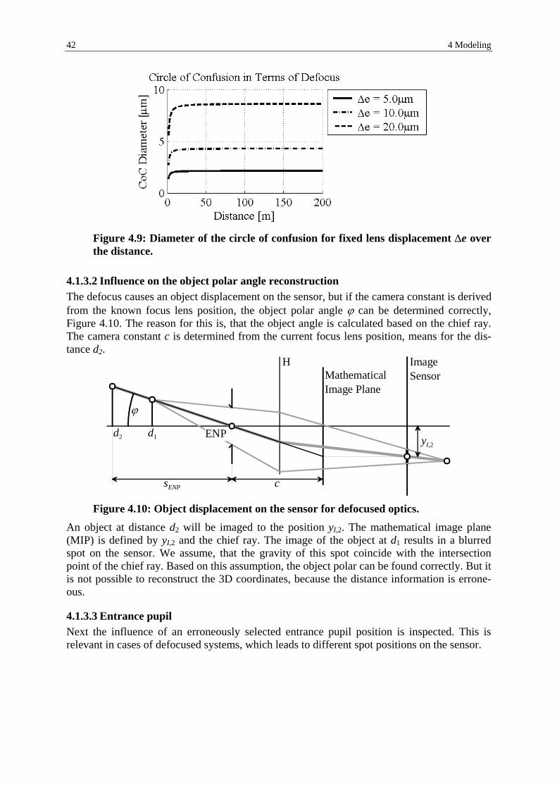
42 4 Modeling

Figure 4.9: Diameter of the circle of confusion for fixed lens displacement ∆e over the distance.

4.1.3.2 Influence on the object polar angle reconstruction The defocus causes an object displacement on the sensor, but if the camera constant is derived from the known focus lens position, the object polar angle ϕ can be determined correctly, Figure 4.10. The reason for this is, that the object angle is calculated based on the chief ray. The camera constant c is determined from the current focus lens position, means for the dis-tance d2.

ImageSensor

HMathematicalImage Plane

ENP

csENP

ϕ

d1d2 yI,2

Figure 4.10: Object displacement on the sensor for defocused optics.

An object at distance d2 will be imaged to the position yI,2. The mathematical image plane (MIP) is defined by yI,2 and the chief ray. The image of the object at d1 results in a blurred spot on the sensor. We assume, that the gravity of this spot coincide with the intersection point of the chief ray. Based on this assumption, the object polar can be found correctly. But it is not possible to reconstruct the 3D coordinates, because the distance information is errone-ous.

4.1.3.3 Entrance pupil Next the influence of an erroneously selected entrance pupil position is inspected. This is relevant in cases of defocused systems, which leads to different spot positions on the sensor.

4.1 Optics and mechanics 43

ImageSensor

HMIP

ENP

csENP

ϕ

d1d2

ENP'

sENP'

MIP'

c'

ϕ'

yI,2

yO,1

yO,2

Figure 4.11: Erroneously entrance pupil position.

The image of the object is constructed using the correct entrance pupil ENP and reconstructed using the erroneously pupil the ENP′. The mathematical image plane is defined by the focus-ing distance d1, the entrance pupil ENP and the chief ray, while MIP’ is defined by the same focusing distance and chief ray, but with ENP′ yielding c′. The object polar angle is defined by the relation between c′ and yI,2. The difference ϕ - ϕ′ is calculated as follows: Correct object angle

( ) ( )11,tan

ENP

O

s

y=ϕ (4.10)

The image is defined by: ( )

( ) 1,1

2

2, OENP

ENP

OI y

s

sxfy ⋅⋅= (4.11)

The camera constant 'c

( ) ( )22

2,

2,' PENO

PENO

I sxfs

yy

c ′′ ⋅=⋅= (4.12)

And finally the object angle for ENP′

( )( )

( ) ( ) 1,21

2

2,

1

'tan

OPENENP

ENP

I

yss

sc

y

⋅⋅=

=′

′

ϕ

(4.13)

where ( )iENPs , ( )i

PENs ′ Distance between the object at distance di and the entrance pupil (Either ENP or ENP′)

f Focal length for focus distance d2 xO Distance between object at distance d2 and focal point f

44 4 Modeling

The angle difference depends on the distance between the correct and the erroneous position of the entrance pupil and on the distance of the object from the optical axis. The farer the ob-ject is from the optical axis, the bigger the error is.

( ) ( )

( )

( )

( )

( ) ( )

( )

−=

−=′−

′

′

′

2

22

11,

2

2

11, 1tan

PEN

ENPPEN

ENP

O

PEN

ENP

ENP

O

s

ss

s

y

s

s

s

yϕϕ

(4.14)

The main lens is the aperture stop for the lens system. Therefore, the entrance pupil equals the aperture stop. But this does not coincide with the standing axis. As stated above, the projec-tion center should be in the intersection of the standing and tilting axis of the theodolite. Hence, we move the ENP artificially into this point and inspect the error of object angle re-construction using formula (4.13), if the image point is 3 mm from the optical axis.

Figure 4.12: Object angle error for ENP in the theodolite origin.

Assuming a focus lens uncertainty of ∆e = 10.0 µm, where the circle of confusion is half a pixel, the object angle error is below 0.05 mgon for a image point at radius 3 mm from the center. Therefore, the assumption that the entrance pupil (Projection center) is located at the theodolite origin is valid.

4.2 Theodolite axes errors Ideally, the theodolite should meet the following requirements: a) Line of sight perpendicular to the tilting axis b) Tilting axis perpendicular to the vertical axis c) Vertical axis strictly vertical d) Vertical-circle reading precisely zero at the zenith If these conditions are not met, the following terms are used to describe the particular errors [Zeiske, 2000] a) Vertical- or height-index error; angle between the zenith direction and the zero reading of

the vertical circle. We will use the symbol e1. b) Line-of-sight error, or collimation error e2; deviation from the right angle between the line

of sight and the tilting axis. We will use the variable e2 instead of the commonly used symbol c to prevent from confusion with the camera constant.

4.2 Theodolite axes errors 45

c) Tilting-axis error; deviation from the right angle between the tilting axis and the vertical axis. We will use the symbol e3.

d) Vertical- or standing-axis tilt; angle between the plumb line and the vertical axis. We will use the symbol e4.

Taking measurements in both telescope faces eliminates the vertical-index, the collimation- and the tilting axis error. Vertical-axis tilt does not rate as being an instrument error; it arises because the instrument has not been adequately leveled up and measuring in both telescope faces cannot eliminate it. Its influence on the measurement of the horizontal and vertical an-gles is corrected by means of the two-axis inclination sensor. The Figure 4.13 depicts the four errors schematically. a) b) c) d)

Figure 4.13: a) Vertical-index error. b) Collimation error. c) Tilting-axis error. d) Vertical- or standing-axis error.

The following description shows, how the influence of those errors can be determined and eliminated [Deumlich & Staiger, 2002]. We will not consider the vertical-axis error, because this error cannot be found a priori by a calibration because it is a setup error. The correction is calculated using the tilt measurement, cf. section 4.3.3. The sign convention for applying the corrections is chosen with respect to the definition used in Leica instruments.

4.2.1 Vertical-index error To compensate the vertical-index error, the vertical angle derived from the theodolite system is corrected by

1, eVV TCT −= (4.15)

where VT Vertical angle measured by the theodolite without any correction (Raw angle)

VT,C Corrected vertical angle e1 Vertical-index error

The determination of the vertical-index error is evaluated with a two face measurement, which should be in the vertical range of 90−110 gon. The mean value of the vertical angles of both measurements equals the vertical-index error.

46 4 Modeling

( ) ( )π−

+=

2

21

1TT VVe (4.16)

where VT(i) Raw vertical angle measured in telescope face i (1 and 2).

The influence of the vertical-index error is independent of the pointing direction, both hori-zontal and vertical angle.

4.2.2 Collimation and tilting-axis error The collimation- and the tilting-axis error both influence only the horizontal angle. The hori-zontal angle is correct by two terms.

( )CTCTTCT V

eVeHzHz

,

3

,

2, tan)sin(

+−= (4.17)

where HzT Horizontal angle measured by the theodolite without any correc-tion (Raw angle)

HzT,C Corrected horizontal angle e2 Collimation error e3 Tilting-axis error

The influence of the collimation error is highest for horizontal pointing, while the tilting-axis error then vanishes. To determine the collimation error a reasonable point is measured in both telescope faces. The vertical angle of the point relative to the horizon should not exceed ± 20 gon. Thus, any influ-ence of the vertical-index error and of the tilting-axis error can be neglected. ( ) ( )( )

2

21

2π+−

= TT HzHze (4.18)

where HzT(i) Raw horizontal angle measured in telescope face i (1 and 2).

Finally, the tilting-axis error can be found by pointing an object at vertical angle of ca. 50 gon in both telescope faces. An important requirement is, that immediately before the tilting-axis error is measured, the collimation error is determined. ( ) ( )( ) ( )( )2

,

2,

1,

3 tan2

22CT

eTeT VHzHz

e ⋅+−

=π

(4.19)

where HzT,e2(i) Horizontal angle measured in telescope face i (1 and 2) and cor-

rected by the collimation error

)sin( ,

2, 2

CTTeT V

eHzHz −=

VT,C(2) Vertical angle in second face fully corrected

4.3 Mapping from sensor plane into object space 47

4.3 Mapping from sensor plane into object space After defining the camera constant in terms of known, fixed or calibration determined pa-rameters we can use the pinhole camera model to derive the mapping function. We will dis-tinguish between an inner orientation, describing the camera to image transformation, and an outer orientation, describing the scene to camera mapping, [Horn, 2000]. The transformation will use theodolite angles and tilt measurements to describe the outer ori-entation. Further the theodolite axis correction terms, vertical-index, collimation and tilting- axis error are used to define the theodolite pointing axis. We must be aware, that the optical axis does not coincide with the theodolite axis. This deviation must be adequately modeled. We have two important points on the sensor, the principal point P, defined by intersection of optical axis with the sensor, and the intersection point TA of the theodolite axis with the sen-sor. Because of mechanical tolerances those two points do not coincide. For reliable polar angle calculation from the object position in the image, we have to know the relative position to the theodolite axis TA. [Huang & Harley, 1989] describes a procedure to calibrate photogrammetric cameras without a control field as long as it can be mounted on the telescope of a theodolite. The principle of this calibration method is used to derive the modeling of the mapping function.

4.3.1 Inner orientation The parameters of the inner orientation of a camera describe the location of the projection center and the deviation from the mathematical model of the central perspective. The camera is a spatial system that consists of the (plane) image sensor and the objective with the projec-tion center. The coordinates of targets measured in digital images refer to the pixel coordinate system.

xP(P)

yP(P) Pixel

psx

psy

P

Y(I)

X(P)

Y(P)

X(I)

Figure 4.14: Pixel and image coordinate system.

A shown in Figure 4.14 the pixel coordinate system is defined as a left handed coordinate system with the point ( )1,1 at the center of the left topmost pixel and with the x-axis parallel to the rows and the y-axis parallel to the columns of the digital image. Image coordinates refer to the right-handed image coordinate system. Its origin is usually placed that it coincides with

48 4 Modeling

the location of the principal point in the image plane, [Bayer, 1992]. The transformation from pixel to image coordinates is defined via the pixel-to-image coordinate transformation: ( ) ( ) ( )( )P

PPI xxpsxx −⋅= (4.20)

( ) ( ) ( )( )PP

PI yypsyy +−⋅= (4.21)

where x(I), y(I) Image coordinates x(P), y(P) Pixel coordinates psx, psy Pixel spacing (Units: mm) xP

(P), yP(P) Location of the principal point in the pixel coordinate sys-

tem (Units: pixel) The parameters of the inner orientation are: • Principal point P:

Intersection of the plumb line trough the projection center with the image plane. • Camera constant c:

This is defined in section 4.1. It specifies the orthogonal distance between the projection center and the principal point. If the optics is focused to infinity, it corresponds approxi-mately to the focal length: c ≈ f

• Parameter describing the optical distortion: [Brown, 1971] defines various parameters describing the radial-symmetric and the ra-

dial-asymmetric and tangential distortion. Especially for CCD cameras, [Bayer, 1992] extended the parameter set with affinity and shear to describe the influence of the im-age digitizer.

[Huep, 1988] proposes, that because of the small field of view compared with photo-grammetric camera systems, the optical distortion has not to be modeled separately.

Thus, we have two possibilities for modeling the deformations caused by optical distortion and mechanical assembly. We can use the traditional approach used in photogrammetry [Gruen & Huang, 2001], using the following individual parameters: • Change of the principal point position • Change of the camera constant • Scale factor (“affinity”) • Shear factor (jointly in x, y) • First three parameters of radial symmetric lens distortion • First two parameters of decentering distortion We will not go into detailed description of these approaches, because it is well known and described in various publications and textbooks, for example [Kraus, 1997; Maas & Nied-eröst, 1997; Luhmann, 2000]. Secondly, a linear function A is used to correct the deformations. The optical distortion (radial symmetrical lens distortion) can be approximated by a linear function resulting in residuals below ± 0.3 µm, for an image radius of 1.8 mm, as can be shown by optical system analysis. Considering the pixels size of 9.8 ×6.3 µm the error due to the linear approximation can be neglected, it is below a tenth of a pixel. This is a consequence of the optic design and of the small field of view. There remain two different error sources causing the deformation of the image. The mechanic assembly can result in a rotation and a tilt of the image sensor. Further a

4.3 Mapping from sensor plane into object space 49

scale difference coming from the pixel size variation. Those influences are modeled by an affine transformation without shift, separated into scale, shear and rotation. ( ) ( )

( ) ( )

−⋅

⋅

=

=

αααα

cossinsincos

101

00

2221

1211 ss

saaaa

y

xA (4.22)

with sx, sy Scale factor in both directions s Shear factor α Rotation angle

The transformation A is a linear function and thus independent of the principal point. We will use lower case letter q describing the undistorted image of the target point Q, while q′ identifies the measured image coordinate including all deformations. The point q corresponds to that position in the sensor plane got by the central projection of the target Q. We must be aware, that the deformation is modeled relative to the principal point, which is the symmetri-cal point of the central projection. The deformations are labeled with ∆ri.

TA

X(I)

Y(I)

TA'

q'

q

P

∆rTA ∆rq

Figure 4.15: Deformation correction in the image plane using affine transforma-tion without shift.

The relation between to position q and q′ is illustrated in Figure 4.15 and given by:

qq rAr ⋅=′ (4.23)

An important point in the image plane is the theodolites crosshair. The pointing direction of the crosshair is defined as invariant in both theodolite faces. That means, the image q′ of any target coinciding with the crosshair TA′ in face one coincides also with TA′ in second face. TA′ describes the location of a target image that is invariant when measuring in both theodolite faces. Because TA′ is defined in the digital image and thus is also distort, as illus-trated in Figure 4.15. Finally, we are interested in the image distance between the TA′ and q′, because this defines the object polar angle relative to the theodolite axis. TA′ can be arbitrarily set, because using the theodolite axis correction terms (vertical-index-, collimation- and tilt-axis-error) the pointing position invariant in both faces can be calibrated to any point in the reticle plane.

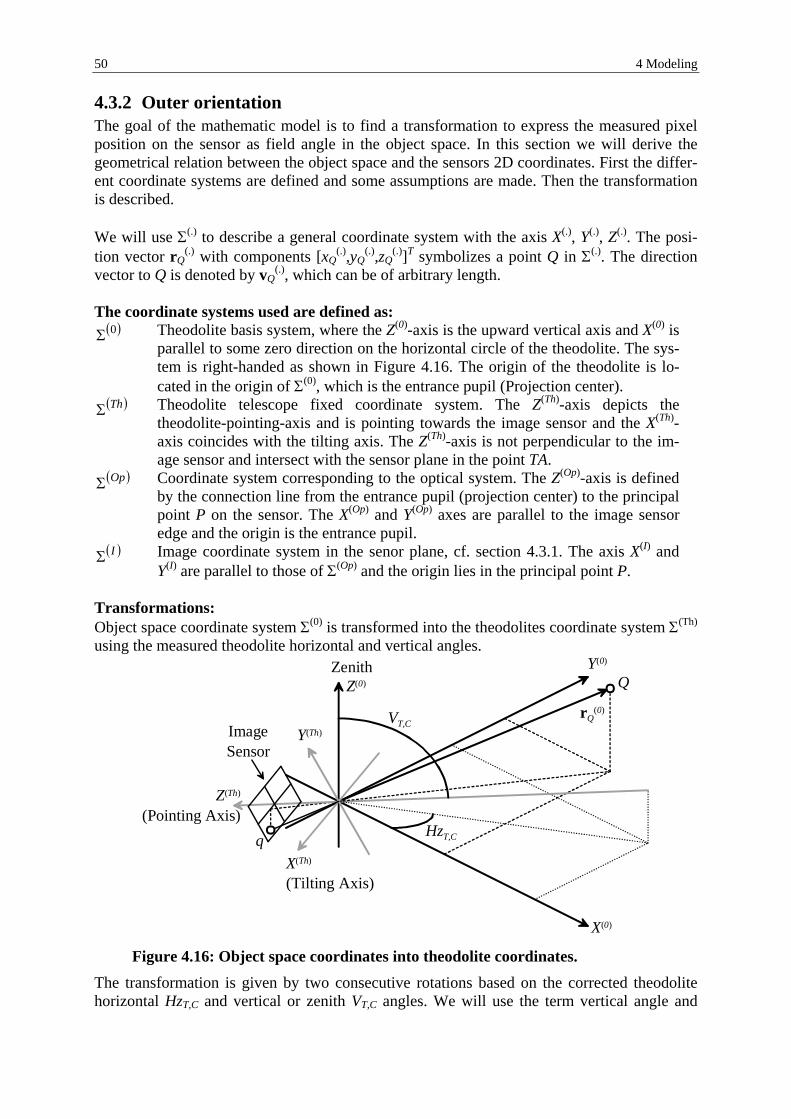
50 4 Modeling

4.3.2 Outer orientation The goal of the mathematic model is to find a transformation to express the measured pixel position on the sensor as field angle in the object space. In this section we will derive the geometrical relation between the object space and the sensors 2D coordinates. First the differ-ent coordinate systems are defined and some assumptions are made. Then the transformation is described. We will use Σ(.) to describe a general coordinate system with the axis X(.), Y(.), Z(.). The posi-tion vector rQ

(.) with components [xQ(.),yQ

(.),zQ(.)]T symbolizes a point Q in Σ(.). The direction

vector to Q is denoted by vQ(.), which can be of arbitrary length.

The coordinate systems used are defined as:

( )0Σ Theodolite basis system, where the Z(0)-axis is the upward vertical axis and X(0) is parallel to some zero direction on the horizontal circle of the theodolite. The sys-tem is right-handed as shown in Figure 4.16. The origin of the theodolite is lo-cated in the origin of Σ(0), which is the entrance pupil (Projection center).

( )ThΣ Theodolite telescope fixed coordinate system. The Z(Th)-axis depicts the theodolite-pointing-axis and is pointing towards the image sensor and the X(Th)-axis coincides with the tilting axis. The Z(Th)-axis is not perpendicular to the im-age sensor and intersect with the sensor plane in the point TA.

( )OpΣ Coordinate system corresponding to the optical system. The Z(Op)-axis is defined by the connection line from the entrance pupil (projection center) to the principal point P on the sensor. The X(Op) and Y(Op) axes are parallel to the image sensor edge and the origin is the entrance pupil.

( )IΣ Image coordinate system in the senor plane, cf. section 4.3.1. The axis X(I) and Y(I) are parallel to those of Σ(Op) and the origin lies in the principal point P.

Transformations: Object space coordinate system Σ(0) is transformed into the theodolites coordinate system Σ(Th) using the measured theodolite horizontal and vertical angles.

X(0)

QZenith Y(0)

Z(0)

Z(Th)

(Pointing Axis)

X(Th)

(Tilting Axis)

Y(Th)

rQ(0)

HzT,C

VT,C

q

ImageSensor

Figure 4.16: Object space coordinates into theodolite coordinates.

The transformation is given by two consecutive rotations based on the corrected theodolite horizontal HzT,C and vertical or zenith VT,C angles. We will use the term vertical angle and

4.3 Mapping from sensor plane into object space 51

zenith angle similarly. It describes the angle measured between the local vertical and the pointing line. The horizontal angle is positive as measured from the X(0)-axis in a clockwise direction seen from the zenith [Torge, 2001].Because of the different orientations of the two coordinate systems, we additionally have to add rotations. Thus, the rotations are defined as: 1. Rotation by −HzT,C − π/2 around the Z(0)-axis 2. Rotation by VT,C + π around the rotated X(0)-axis (by step 1) The additional terms −π/2 and π are to provide that the Z(Th)-axis points toward the image sen-sor. The rotation is calculated as: ( ) ( )

( ) ( )( ) ( )

( ) ( )( ) ( )

( )

( ) ( ) ( ) ( ) ( )( ) ( ) ( ) ( ) ( )

( ) ( )( )ThQ

CTCT

CTCTCTCTCT

CTCTCTCTCT

ThQ

CTCT

CTCT

CTCT

CTCT

ThQVHzQ

VVVHzVHzHzVHzVHzHz

VVVV

HzHzHzHz

CTCT

r

r

rRRr

⋅

−−

−−−=

⋅

−−−

⋅

−−

−=

⋅⋅= +−−−

,,

,,,,,

,,,,,

,,

,,

,,

,,

20

cossin0sinsincossincossincoscoscossin

cossin0sincos0

001

1000sincos0cossin

,,

K

ππ

(4.24)

( ) ( )ThQQ rRr ⋅=0 (4.25)

In the following we are only interested in the pointing vector towards point Q, because the distance information is not a priori available.

( )( ) ( )( ) ( )

( )

⋅−⋅

=

Q

QQ

QQ

QVVHzVHz

cossinsinsincos

0v (4.26)

And using the rotation yields: ( ) ( )

( ) ( ) ( ) ( ) ( )( ) ( ) ( ) ( ) ( )( ) ( ) ( ) ( ) ( )

+⋅−⋅+⋅−⋅+⋅−⋅

=

⋅=

QQQQQ

QQQQQ

QQQQQ

QTTh

Q

VrVHzrVHzrVrVHzrVHzrVrVHzrVHzr

coscossinsincoscoscossinsincoscoscossinsincos

332313

322212

312111

0vRv

(4.27)

where rij coefficients of the rotation matrix R The projective transformation must be performed relative to the optical axis that means the axis perpendicular to the image plane through the principal point P and the entrance pupil. From the calculation above we know the pointing direction of the theodolite given by the axis Z(Th). This coordinate system must be rotated that the Z(Th)-axis coincide with the optical axis Z(Op). The relations are defined in Figure 4.17.

52 4 Modeling

rq(I)

QrQ

(Th)

Z(Th) SensorPlane

TAY(Op)

ν

µZ(Op)

X(Op)

X(Th)

Y(Th)

-c P

ν

µ

q

X(I)

Y(I)

rTA(I)

Figure 4.17: Theodolite coordinates into optical system coordinates.

The intersection of the theodolite pointing axis Z(Th) with the image plane defines the not dis-tort position of the crosshair TA. The theodolite coordinate system Σ(Th) must be rotated, that the Z(Th)-axis coincide with the Z(Op)-axis. This rotation is given by first rotating around X(Th)-axis by angle ν followed by a rotation around the rotated Y(Th)-axis by the angle µ. ( ) ( )

( )

( ) ( )( ) ( )

( ) ( )

( ) ( )( )

( ) ( )( ) ( ) ( ) ( ) ( )( ) ( ) ( ) ( ) ( )

( )OpQ

OpQ

OpQOp

OpQ

ThQ

r

r

rR

rRRr

⋅

−−=

⋅

−⋅

−=

⋅=

⋅⋅=

µννµνµννµν

µµ

µµ

µµ

νννν

µν

coscossinsincoscossincossinsin

sin0cos

cos0sin010

sin0cos

cossin0sincos0

001

(4.28)

The position of TA can be calculated using the affine transformation without shift describing the deformation derived in section 4.3.1. ( ) ( )

( )

( )

=

⋅= ′−

ITA

ITA

IAT

ITA

yx

1Ar

(4.29)

Thus, the rotation angles are define

( )( )

cx I

TA=µtan (4.30)

( )

( )

( ) 22tan

cx

y

ITA

ITA

+

−=ν (4.31)

4.3 Mapping from sensor plane into object space 53

Because of the small field of view and the mechanical adjustment, the angles ν and µ are small. Therefore, we are allowed to do the following simplifications: ( )

( )( ) µµ

µµµ

===

tansin

1cos

( )( )( ) νν

ννν

===

tansin

1cos

The simplified parameter of the rotation are then found by:

( )

( ) ( ) ( )

( ) ( )

( )

( )

( ) ( )

−−

≈

−−

⋅−=

−−⋅≈

1

10

01

1

1

01

1101

2

cy

cx

cyc

x

cy

cx

cy

cyx

cx

ITA

ITA

ITA

ITA

ITA

ITA

ITA

ITA

ITA

ITA

Op

νµνµν

µR

(4.32)

The projective transformation of the target point Q yields the image point q in the image plane. In analogy to the collinearity equations we find:

( )

( )

( )

( )

( )ThQ

TOp

OpQ

Opq

Opq

Opq

m

m

cyx

rR

r

r

⋅⋅=

⋅=

−=

(4.33)

where ( ) ( )

( ) ( )Opq

Iq

Opq

Iq

yy

xx

=

=

54 4 Modeling

The relation ( )OpQzc

− defines the scaling factor m. Using all the formulas from above, the im-

age coordinates can be derived: ( ) ( )

( )

( )

( )

( )( )

( )

( )( )

( )( )

( )ThQ

ITATh

Q

ITATh

Q

ThQ

ITATh

Q

OpQ

OpQ

OpQ

Opq

Iq

yc

yx

cx

z

zc

xx

c

z

xc

xm

xx

⋅+⋅+

⋅−⋅−=

⋅−=

⋅=

=

(4.34)

( ) ( )

( )

( )

( )

( )( )

( )

( )( )

( )( )

( )ThQ

ITATh

Q

ITATh

Q

ThQ

ITATh

Q

OpQ

OpQ

OpQ

Opq

Iq

yc

yx

cx

z

zc

yy

c

z

yc

ym

yy

⋅+⋅+

⋅−⋅−=

⋅−=

⋅=

=

(4.35)

Those formulas can further be simplified. xQ

(Th) and yQ(Th) are at least 76 times smaller than

zQ(Th) because of a maximal field of view of 1.66 gon. Therefore, the terms

( )( )ThQ

ITA xc

x⋅ and

( )( )ThQ

ITA yc

y⋅ in the denominator can be neglected. Note this assumption is only valid for the

actual theodolite optics of the Leica TPS1100 series. If the field of view changes, this has to be checked. This simplification yields the formulas for calculating the image coordinate of the target point.

( )( )

( )( )ITATh

Q

ThQI

q xz

xcx −⋅−= (4.36)

( )

( )

( )( )ITATh

Q

ThQI

q yz

ycy −⋅−= (4.37)

As already noted, because the deformation is a linear function, the position of the principal point has no influence on the result, as can be seen in the following calculation:

4.3 Mapping from sensor plane into object space 55

( ) ( )( )

( )

( )( ) ( )( )

( ) ( )( )( )

( )

( )( )

( )ThQ

ThQI

TAq

ThQ

ThQP

TAP

q

PP

PTATh

Q

ThQP

PP

q

z

xcx

z

xcxxpsx

xxpsxz

xcxxpsx

⋅−=

⋅−=−⋅

−⋅−⋅−=−⋅

,

(4.38)

( )( )

( )ThQ

ThQI

TAq z

ycy ⋅−=, (4.39)

where ( )ITAqx , , ( )I

TAqy , Difference vector between the target point and the cross-hair position. It is directed from the crosshair to the target point.

Remark: This simplification under the assumption that the field of view is small means, that the rota-tion ROP has been replaced by a translation TOP: ( ) ( )

( )ThQOp

ThQ

TOp

Opq

m

m

rT

rRr

⋅′+≈

⋅⋅=

(4.40)

where OpT ( ) ( )[ ]TI

TAI

TA yx 0

m ( )OpQzc

−

=′m ( )ThQzc

−

Summarizing all transformations: Finally, the relation between object in the 3D space and the measured object point in the im-age is given by

( ) ( )( ) ( )

( )ThQ

ThQ

ThQTA

qI

ATq z

yaxacxx

⋅+⋅⋅−== ′′′

1211, (4.41)

( ) ( )

( ) ( )

( )ThQ

ThQ

ThQTA

qI

ATq z

yaxacyy

⋅+⋅⋅−== ′′′

2221, (4.42)

56 4 Modeling

4.3.3 Tilt correction The TPS1100 Professional Series Total Station is equipped with a two-axis tilt sensor. This sensor provides a tilt measurement relative to the current pointing direction, longitudinal tilt, and orthogonal thereto, lateral or transverse tilt. Using the tilting angles to calculate the in-cline plane:

CTT

LP

TLA

HzII

I

III

,

22

arctan −

=

+= (4.43)

where IL Longitudinal inclination angle (in pointing direction). IT Transverse inclination angle. HzT,C Horizontal angle of the pointing direction (Corrected by the axis

errors). The inclination angles for the new pointing direction HzQ is then given by: ( )

( )CQPAQT

CQPAQL

HzIII

HzIII

,,

,,

cos

sin

+⋅=

+⋅= (4.44)

And finally the corrected horizontal and vertical angles of the target can be calculated as:

( )CQQTQCQ

QLQCQ

VIHzHz

IVV

,,,

,,

cot⋅+=

+= (4.45)

The vertical angle is directly influenced by the longitudinal tilt, while the transverse tilt and the corrected vertical angle are used to correct the horizontal angle. The subscript I denotes an incline corrected angle.

4.3.4 Summarizing the transformations To determine the object polar angle in the superior coordinate system, all the transformations from the previous sections must be linked to get the transformation from image space into 3D space, which we will call back-transformation. It will only be possible to reconstruct the object polar angles and not the 3D coordinates, because the optics magnification is not known accurately enough. Hence we will derive a transformation describing the calculation of the fully corrected object polar angles HzQ,C and VQ,C given in the coordinate system Σ(0) from the measured target position rq′

(P) in the pixel coordinate system Σ(P). The direction vector vQ

(Th),which is not incline corrected, is used to derive the transformation. It is defined as shown in Figure 4.18 and expressed by the formula below

( )

( )

( )

−=

cy

xITAq

ITAq

ThQ ,

,

v

(4.46)

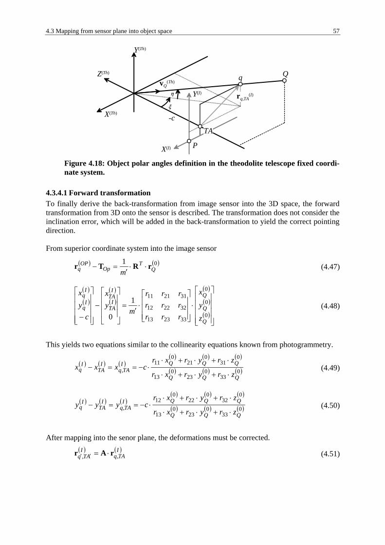
4.3 Mapping from sensor plane into object space 57

vQ(Th)

qZ(Th)

X(Th)

Y(Th)

X(I)

Y(I)

Q

-cξ

η

P

rq,TA(I)

TA

Figure 4.18: Object polar angles definition in the theodolite telescope fixed coordi-nate system.

4.3.4.1 Forward transformation To finally derive the back-transformation from image sensor into the 3D space, the forward transformation from 3D onto the sensor is described. The transformation does not consider the inclination error, which will be added in the back-transformation to yield the correct pointing direction. From superior coordinate system into the image sensor

( ) ( )01Q

TOp

OPq m

rRTr ⋅⋅′

=− (4.47)

( )

( )

( )

( )

( )

( )

( )

⋅

⋅

′=

−

− 0

0

0

332313

322212

3121111

0Q

Q

QI

TA

ITA

Iq

Iq

z

y

x

rrrrrrrrr

myx

cyx

(4.48)

This yields two equations similar to the collinearity equations known from photogrammetry.

( ) ( ) ( )( ) ( ) ( )

( ) ( ) ( )033

023

013

031

021

011

,QQQ

QQQITAq

ITA

Iq

zryrxr

zryrxrcxxx

⋅+⋅+⋅

⋅+⋅+⋅⋅−==− (4.49)

( ) ( ) ( )

( ) ( ) ( )

( ) ( ) ( )033

023

013

032

022

012

,QQQ

QQQITAq

ITA

Iq

zryrxr

zryrxrcyyy

⋅+⋅+⋅

⋅+⋅+⋅⋅−==− (4.50)

After mapping into the senor plane, the deformations must be corrected. ( ) ( )I

TAqI

ATq ,, rAr ⋅=′′ (4.51)

58 4 Modeling

( ) ( ) ( )

( ) ( ) ( )STAq

STAq

SATq

STAq

STAq

SATq

yaxay

yaxax

,22,21,

,12,11,

⋅+⋅=

⋅+⋅=

′′

′′ (4.52)

And finally the transformation into the pixel coordinate system is calculated

( ) ( ) ( ) ( )

( ) ( ) ( ) ( )IATq

PAT

Pq

PATq

IATq

PAT

Pq

PATq

ypsy

yyy

xpsx

xxx

′′′′′′

′′′′′′

⋅=−=

⋅=−=

,,

,,

1

1

(4.53)

The position (xTA′

(P), yTA′(P)) of the crosshair TA′ can be freely defined and is normally placed

in the central pixel of the image sensor.

4.3.4.2 Backward transformation The goal of the back-transformation is to find the direction vector to the target point in 3D from the measured image position. For reconstruction, only the difference vector between the crosshair and the target image point has to be used. From a position measurement in the 2D image plane only two parameter of the 3D coordi-nates can be derived. The third dimension is obtained by using the EDM. The incline cor-rected direction vector vQ,C

(0) is specified by the polar angles of the object point Q and ex-pressed by the following relation:

( )( ) ( )( ) ( )

( )

⋅−⋅

=

CQ

CQCQ

CQCQ

CQVVHzVHz

,

,,

,,0,

cossinsinsincos

v (4.54)

Pixel-to-Image coordinate transformation ( ) ( ) ( )( )P

ATP

qI

ATq xxpsxx ′′′′ −⋅=, (4.55)

( ) ( ) ( )( )PAT

Pq

IATq yypsxy ′′′′ −⋅=, (4.56)

Note, that the position of the distort crosshair AT ′ is arbitrary selected. Deformation correction ( ) ( )I

ATqITAq ′′

− ⋅= ,1

, rAr (4.57)

where ( ) ( ) ( )[ ]TIATq

IATq

IATq yx ′′′′′′ = ,,,r (4.58)

4.3 Mapping from sensor plane into object space 59

From 2D image coordinates into the 3D theodolite fixed coordinate system We are only interested in the direction vector vQ

(0). Thus, the direction vector in the theodolite fixed coordinate system is given by:

( )( )

( )Thq

ThqTh

Qr

rv = (4.59)

where ( ) ( ) ( )[ ]TITAq

ITAq

Thq cyx −= ,,r (4.60)

From the 3D theodolite fixed into the superior coordinate system The theodolites horizontal and vertical angles define this transformation. ( ) ( )Th

QQ vRv ⋅=0 (4.61)

where ( ) ( ) ( ) ( )[ ]TzQyQxQQ vvv 0,

0,

0,

0 =v

The polar angles of the object point Q are given by ( )

( )

−= 0

,

0,arctanyQ

yQQ

v

vHz (4.62)

( ) ( )

( )

+

−= 0,

20,

20,arctan

2zQ

yQxQQ

v

vvV π

(4.63)

But in case of an instrument tilt, corrections due to the inclination must be added.

( )( )CQQTQ

CQQCTT

LTLQCQ

QLQ

QCTT

LTLQCQ

VIHz

VHzHzIIIIHzHz

IV

HzHzIIIIVV

,,

,,22

,

,

,22

,

cot

cotarctancos

arctansin

⋅+=

⋅

+−

⋅++=

+=

+−

⋅++=

(4.64)

And finally, the Cartesian coordinates are given by ( ) ( ) ECQCQ StHzVdE +⋅⋅= ,, sinsin (4.65)

( ) ( ) NCQCQ StHzVdN +⋅⋅= ,, cossin (4.66)

( ) THCQ HStVdH ++⋅= ,cos (4.67)

60 4 Modeling

where iSt Station coordinates; i = {E, N, H}

TH Theodolite height over the station point d Object distance

Using these formulas, we are able to calculate 3D coordinates of any point measured in the image, provided that the distance to the object is available. If no distance information is to be used, then only the polar angles of the object can be reconstructed.

4.4 Accuracy considerations The accuracy of the system depends on the accuracy of the single sensors. The IATS has two additional sensors compared with a traditional total station, the image sensor and the focus lens motor. We will evaluate the influence of the focus lens positioning accuracy on the de-terminable accuracy of the object polar angle. The results of this evaluation are used to check the calibration parameter. Further, error propagation for the whole system is calculated to de-termine the influence of the single sensors to the final 3D error. Especially the influence of the new sensors is of interest.

4.4.1 Focus lens positioning The position of the focus lens is used to calculate the camera constant for the actual optics configuration, section 4.1. Here we will derive the influence of the focus lens position to the calculation of the camera constant and finally to the object polar angle. Further it is derived, how accurate the calibration of the mechanics and optics parameter must be to satisfy an an-gular accuracy of 0.3 mgon. The error calculation presented bases on Gaussian error propaga-tion. The camera constant equals the product of the magnification and the distance between the entrance pupil and the object.

ENPsc ⋅= β (4.68)

Further, the camera constant c can be calculated in terms of the encoder position p, the en-coder origin position OL, the gradient SL of the encoder gear and the distance LS between the rear principal plane of the front lens and the image sensor as defined in section 4.1.1. The polar angle depends on the camera constant and the object position in the image and thus is independent of the object distance. The evaluation is done in 1 dimension for the sake of sim-plicity.

ImageSensor

ENPPointing Axis ϕ

c

yI

sENP

yO

Figure 4.19: Relation between object polar angle, camera constant and object posi-tion in the image in one dimension.

4.4 Accuracy considerations 61

The object polar angle is due to the field of view smaller than 0.83 gon (Half field of view). Therefore, we are allowed to replace tan(ϕ) by ϕ. The relation between polar angle, camera constant and radial position yI in the image is given by:

cyI=ϕ

(4.69)

Using the relation above, the error propagation with respect to the polar angle ϕ is calculated:

22

⋅

∂∂

+

⋅

∂∂

= cyI cy I

σϕσϕσϕ

(4.70)

The standard deviation of the object position

Iyσ in the image depends on the image process-ing algorithms. The LSM provides an accuracy of better than 1.0 pixel in real environment [Gruen & Stallmann, 1993]. Because of the different pixel dimension this equals an accuracy of 0.7 to 1.0 µm. We are interested in the required standard deviation of the camera constant satisfying the re-quired standard deviation of the polar angle. Separating σc in the above equation we get:

222Iy

Ic c

yc σσσ ϕ −⋅⋅= (4.71)

The standard deviation of the camera constant is numerically calculated using an object point in the image at position yI = 1.8 mm, which equals the radius of the maximal possible circle on the image sensor. The calculations are done for two different assumptions for the localiza-tion accuracy of the target in the image to meet the different pixel size on both dimensions. The standard deviation of the polar angle ϕ is set to 0.3 mgon.

Figure 4.20: Maximum σc for different localization accuracies to fulfill the re-quirements of the polar angle accuracy.

In Figure 4.20 the maximal allowed standard deviation for the camera constant in terms of the target position on the image and the required polar angle accuracy is given. We can derive, that the standard deviation of the camera constant should be below 100 µm.

62 4 Modeling

The standard deviation of the camera constant is defined via the standard deviations of the optical-mechanical parameters. Error propagation for c using formula (4.8) yields: 2222

2

⋅

∂∂

+

⋅

∂∂

+

⋅

∂∂

+

⋅

∂∂

=SLLL L

SS

LO

Lpc L

cSc

Oc

pc σσσσσ (4.72)

And with numerical calculation of the derivatives we get: ( ) ( ) ( ) ( )2224242 78.207.0105.8105.8

SLLL LSOpc σσσσσ ++⋅+⋅= −− (4.73)

The result of this evaluation will be used to quantify the results of the estimation of the optics-mechanics parameters described in section 6.2. It is assumed that all parameters contribute the same amount to the variance of the camera constant. Thus, we get

jc

jc

σσ

σσ

⋅=

⋅=

2

4 22

(4.74)

where σj2 Variance of each parameter weighted with the derivative of

the camera constant function From these calculations the required standard deviation of each parameter under the assump-tion of contributing the same amount to the final error can be found.

mm018.0

step/mm8.0

step60

step60

=

=

=

=

S

L

L

L

S

O

p

σ

σ

σ

σ

Those results are used in the following to check the results of the camera constant calibration. We made the assumption, that all parameters contribute the same amount to the final error. If in the calibration of any parameter can be determined much more precisely than required in the above specification, the requirements of the other parameters can be relaxed.

4.4.2 Theodolite sensors Based on the back-transformation including the tilt correction, the distance measurement and the theodolite station setup, the error propagation related to 3D coordinate calculation is evaluated. The purpose of this is to get an idea of how the new sensors, the camera and the motorized focus lens, influence the overall measurement error. The Cartesian coordinates defined in formulas (4.65) – (4.67) are extended by the setup error due to the laser plummet variation. ( ) ( ) LPStHzVdE EICQICQ ++⋅⋅= ,,,, sinsin (4.75)

4.4 Accuracy considerations 63

( ) ( ) LPStHzVdN NICQICQ ++⋅⋅= ,,,, cossin (4.76)

( ) THICQ HStVdH ++⋅= ,,cos (4.77)

where Sti Station coordinates; i = {E, N, H} LP: Setup error in the horizontal plane due to laser plummet (LP)

deviation from the plumb line HT Theodolite height over the station point

To calculate the final error we first have to define the accuracy of the single sensors and measurement.

4.4.2.1 Definition of the sensor contributing to 3D coordinate calculation The coordinates, Easting, Northing and Height, depend on various sensor measurements, which will be described in the following. The accuracies given are extracted from [Leica, 2003] if not otherwise stated. Measuring the object position in the image The object position is determined using least squares template matching, cf. section 5.2.3, where we can assume to get an accuracy of object localization of 0.1 pixels. Because the pixel size differs in both directions by a factor 1.5, we will define the standard deviation not in pixel but in mm. The standard deviation in x- and y-direction is chosen with 1.0 µm. This equals an accuracy of 0.1 and 0.16 pixels, respectively. Camera constant In section 4.4.1 we derived that the accuracy of the camera constant should be below 100 µm to get an angular accuracy of 0.3 mgon. The online calibration of the camera constant, which is explained later in section 6.2, yields an accuracy of 60 µm. This fulfills the expectations and thus will be used to in the error propagation. Theodolite angle measurement The angular accuracy of the TPS1100 series type 1101 is given with 0.5 mgon. This accuracy is determined according the definition of [ISO 17123-3, 2001]. The accuracy is derived from manually measuring several targets in both telescope faces. Thus, the specified standard de-viation include different error sources, such as raw angle measurement, user pointing capabil-ity etc. But at the same time, the accuracy is determined by averaging using two-face meas-urement and multiple measurement of the same target. For the error propagation, we need a standard deviation describing the raw angle measurement. We will choose the raw angle accu-racy as 0.3 mgon. This value is confirmed by the theodolite calibration described later in sec-tion 6.3. Theodolite inclination measurement The setting accuracy of the dual axis compensator is given with 0.2 mgon for Leica Total Sta-tions Type 1101 and 1102. Electronic laser distance measurement (EDM) The instrument is equipped with an extended range distance measurement system based on a special frequency measurement system using a visible red laser. The accuracy for a reflector-free measurement is specified with 3 mm + 2 ppm. Beam interruptions, severe heat shimmer

64 4 Modeling

and moving objects within the beam path can result in deviations of the specified accuracy. The distance range for measuring is up to 170 m for a white target under good atmospheric conditions. Usually, the working range is up to 100 m. Because variable error of 2 ppm corre-sponds to only 0.2 mm at 100 m we will neglect it. The standard deviation used for error propagation is 3 mm. Laser plummet The laser plummet is used to setup the instrument over a defined ground point. Any deviation from the plumb line yields a setup error, which influences the 3D coordinates. The deviation from the plumb line at 1.5 m height is specified with LP = 0.75 mm. This deviation represents a radius of a circle around the ground point. Consequently we should use the term LP⋅sin(HzQ,C) in the Easting and the term LP⋅cos(HzQ,C) in the Northing calculation. But for simplicity we only use the additional term LP. Station height measurement The station height above the ground point is measured manually using a meter. Due to the bending of the meter and the height reading we assume a standard deviation of the height measurement of 0.5 mm. Summarizing Table 4.3 summarizes the single sensor measurement and the corresponding standard devia-tion to use for the error calculation. Description Symbol Standard deviation Object position in the image

x coordinate xq′ 1.00 µm y coordinate yq′ 1.00 µm

Camera constant C 0.06 mm Theodolite angle measurement

Horizontal angle HzT 0.30 mgon Vertical angle VT 0.30 mgon

Theodolite inclination measurement Longitudinal IL 0.20 mgon Transversal IT 0.20 mgon

Reflectorless distance measurement D 3.00 mm Laser plummet LP 0.75 mm Height measurement of the total station TH 0.50 mm

Table 4.3: Defining the values and their standard deviation used to calculate the 3D coordinates.

4.4.2.2 Calculating the over all error in terms of the single sensor error The variance of the single parameters E, N and H can be calculated using again Gaussian error propagation.

4.4 Accuracy considerations 65

222

222

,

2

,

22

222

,,

∂∂℘

+

∂∂℘

+

∂∂℘

∂∂℘

+

∂∂℘

+

∂∂℘

+

∂∂℘

+

∂∂℘

+

∂∂℘

+

∂∂℘

=′′

′′℘

T

TLCTCT

qqq

HT

LPd

IT

IL

VCT

HzCT

cyyq

xq

HLPd

IIVHz

cyx

σσσ

σσσσ

σσσσσ

K

K

(4.78)

where ℘ Substitute for the functions for calculating Easting, Northing and Height defined at the beginning of the section.

The standard deviation of each dimension depends differently on the parameters. To give an overall specification of the accuracy we will use the joint standard deviation, which we will define as:

222HNEENH σσσσ ++= (4.79)

Further we are also interested in the variance of the polar angles HzQ,C,I and VQ,C,I derived from the image measuring. The distance measurement and the setup error is not included there.

222

,

2

,

22

222

,,

∂∂℘

+

∂∂℘

+

∂∂℘

+

∂∂℘

+

∂∂℘

+

∂∂℘

+

∂∂℘

=′′

′′℘

TLCTCT

qqq

IT

IL

VCT

HzCT

cyyq

xq

IIVHz

cyx

σσσσ

σσσσσ K

(4.80)

where ℘ Substitute for the functions for calculating HzQ,C and VQ,C For the numerical evaluation we use the standard deviation of the single measurement pa-rameter as defined in Table 4.3. The values for the object position in the image are chosen in the sensor center and at 2.2 mm diagonally away from the center. The theodolite angles for HzT are selected in the range of 0-20 gon and for vertical angle VT in the range of 80-100 gon. Inclination is assumed to be between 0 and 100 mgon. The distance used is 100 m and the station position is set to zero in all three dimensions. We get the standard deviation for the single coordinates E, N and H, for the joint standard deviation for σENH and for the corrected horizontal and vertical errors as shown in Table 4.4. The standard deviation in Northing direction is significant higher than the others. This is be-cause the pointing direction is towards Northing and therefore, influenced mainly by the dis-tance measurement, which has the highest uncertainty. The joint error is slightly worse then the distance measurement. Also the horizontal and vertical angles are worsening only by a factor 1.5 compared with the raw angle measurement.

66 4 Modeling

Parameter Standard deviation [mm]

Parameter Standard deviation[mgon]

Eσ 1.0 – 1.3 CQHz ,

σ 0.43

Nσ 2.8 – 3.0 CQV ,

σ 0.47

Hσ 0.9 – 1.2

ENHσ 3.4

Table 4.4: Standard deviation of the 3D Cartesian coordinates and the polar angles for the numerical calculation for a distance of 100 m.

It is interesting to inspect the contribution of each parameter to the final variance. Table 4.5 shows the percentage of each parameter, where the parameters with the highest influence are marked in gray.

% xq′ yq′ c HzT VT IL IT d PL HT 2ENHσ 1.8 1.8 0.3 1.9 2.0 0.9 0.0 79.2 9.9 2.22

,CQHzσ 47.2 0.0 3.4 48.5 0.0 0.0 0.9 - - -2

,CQVσ 0.0 39.6 2.9 0.0 43.1 14.4 0.0 - - -

Table 4.5: Contribution of each parameter to the overall variance. When calculating the Cartesian coordinates E, N and H the influence of the reflectorless dis-tance measurement device becomes significant. The result of the image processing influences the horizontal and vertical angles with about 40−50%.

5 Measurement algorithms Objects of different shape and structure will be measured by the IATS. It is the underlying idea to decompose objects of high complexity into basic geometric primitives, which can be treated with algorithms of reasonable complexity. In this study, we limit our considerations to discs and objects with linear boundaries. Thus the geometric primitives will be a line or a line segment and a disc. The line is defined by an in-tensity edge in the image. The disc object is mainly used for measurements with reference targets. The disc is chosen because of its symmetry and because it can be easily identified automatically in the image, for example by cross-correlation [Lewis, 1995; Haralick & Shapiro, 1992]. The majority of objects structures are defined by line boundaries. Very often an object point can be defined by the intersection of two boundary lines in a natural scene, for example a window frame, a door or a roof. For small objects where it might be difficult to find two inter-secting lines, we use a corner as dedicated geometric primitive. Two quasi-parallel lines de-fine objects, such as tubes, street lamps or pillars. If those boundaries are found, then the cen-tral line can be extracted to specify the pole direction vector. To provide a 3D measurement, the distance to the object has to be measured in addition to the angles, for which we will use the internal reflectorless EDM. It is necessary to know exactly from where the distance is measured. In particular with objects that exhibit changes of depth information due to changes on the object boundary, the EDM laser beam must be pointed ex-actly to a well defined planar surface rather than to an edge to prevent a loss of laser energy or to avoid multiple target situations [Deumlich & Staiger, 2002]. In section 5.1 we outline the basic algorithm of measuring objects. An example of measuring a point defined by two intersecting lines on a stucco wall, Figure 5.1, will be used to illustrate the algorithms. Subsequently, we give a more detailed discussion of the algorithms in sec-tion 5.2. The chapter ends presenting some cases in section 5.3 and conclusions in section 5.4.

Corner point tobe measured

Figure 5.1: Example for measuring a corner point on a stucco wall.

68 5 Measurement algorithms

5.1 Basic approach The procedure for measuring non-cooperative, but natural objects is independent of their structure. It is based on four main tasks: • Object identification in the image • Rough localization with pixel accuracy • Accurate localization with sub-pixel accuracy → yields the Hz and V angle • Measuring the object distance → yields the third dimension There are many possibilities to detect the object in the image. A wide field of research focuses on object recognition [Castleman, 1996]. However, it is extremely difficult to automatize the object identification in a reliable way because of the wide range of different objects. Thus, this study does not deal with object recognition algorithms. Alternatively, the user selects the objects manually. Similar to the measurement with a total station, we are interested in measuring object points. We employ two possible schemes to define these points: 1. The user interactively places multiple lines or a polyline in the image to define the object.

The corners of the polyline, the line intersections or the centerline of two parallel lines specifies the point(s) to be measured in 3D.

2. The user interactively clicks on the point to be measured, and then automatic edge/line detection is performed. All possible line combinations that intersect in the proximity of the desired object point are displayed. The user selects the lines that define the desired target point.

The second approach requires basic image recognition algorithms and thus slows down the execution. Further, the possibility to produce a huge set of line connections from which the correct one must be selected complicates the interaction process. Thus, we will only focus on the simpler and more adequate first approach. The flowchart in Figure 5.2 describes the individual steps measuring non-cooperative object points. In the following, we outline those steps in detail, where the heading lines define the four main tasks described in detail in section 5.2. • Object approximation by manually placing approximate lines The user identifies the object point to be measured in the image. The intersection of

two manually placed lines or the corner point of a polyline defines the point to be measured. For a circular object, the user places a circle where the circle center defines the desired point. The manually placed lines, named approximate lines (AL), ap-proximate objects, which finally define the point.

• Rough object determination, based on edge detection An appropriate edge detection algorithm determines intensity changes near the AL.

Those edge pixels describe the object in the image. Edge pixels are linked to form continuous lines. The algorithm extracts the lines matching the object the best. If there are ambiguities

the user can select the valid lines manually. Analyzing the intensity profile perpendicular to the line results in type and thickness

of the line (not always needed).

5.1 Basic approach 69

• Accurate object reconstruction, based on matching techniques and fitting Applying matching procedures determines the object boundary with sub-pixel accu-

racy. Thus, the exact position of many object points is known. Underlying a formal description (modeling) of the object, we will only focus on linear

objects, where a geometrical structure can be fitted into the boundary points. For linear objects, a straight line is fitted. The residuals of the fit can be used for outlier detection and elimination.

The intersection or corner point, known with sub-pixel resolution, describes the object position in the image. Based on the back-transformation the horizontal and vertical angles can be found.

• Distance measurement Finally, to get the third dimension of the object point, the distance is measured. The

position where to measure the distance can be on the object point, using the Hz and V angle, or it can be defined interactively.

Calculate intersection pointof the fitted lines

=> Hz and V angles

Place approximatelines (AL) to describe

the point to be measured

Find edge pixels inthe image that

describe the object

Combine edge pixelsto lines

Determine lines thatdescribe the object best

Analyze profile perpendicularto the line to determine the

line type and thickness

Local matching to determinethe object boundary with

sub-pixel resolution

Fit straight lines intoboundary pixels

Measure distance ofobject point=> Distance

Figure 5.2: Flowchart describing the basic approach for measuring non-cooperative object points that are defined by intersecting lines or by corner points.

In the ongoing sections we will focus on details of the individual parts of the measurement procedure.

70 5 Measurement algorithms

5.2 Algorithms used for measuring objects This section describes the algorithms defined in the previous section in detail. It is divided into the four main tasks, object approximation, rough and accurate object localization and the distance measuring.

5.2.1 Object approximation The user approximates the object to be measured by manually placing lines in the image. An image is recorded and displayed on the screen. In the prototype solution we use a PC monitor, but later on it will be displayed on any graphic screen such as Handheld-PC or Tablet-PC. The user draws the line using a mouse or a pen. The result of placing a line is shown in Figure 5.3 a) b)

Figure 5.3: Image with manually placed lines approximating the object. a) Show-ing the zoom range. b) Detailed view.

5.2.2 Rough object determination Before the object position can be determined with sub-pixel accuracy, it must be roughly de-tected. Based on the knowledge of the approximate object position in the image from the AL combined with edge detection algorithms with pixel accuracy the object is localized.

5.2.2.1 Edge detection and line segment extraction The object to be measured is described by its boundary lines. Therefore, it is necessary to ex-tract those boundaries, represented as an intensity edge, in the pixel image. Much research work on edge detection was reported in the past, e.g. [Marr & Hildreth, 1980; Haralick, 1984; Perona & Malik, 1991; Heitger, 1995]. The existing approaches cover a wide variety of strategies, using different filter techniques. [Ziou & Tabbone 1998] gives an over-view about common edge detection techniques. For our approach, it is evident to know not only the edge strength but also the edge direction. Thus, we will use the Canny edge detection algorithm [Canny, 1986]. The technique developed in a previous project (AMOBE; Institute of Geodesy and Photo-grammetry, ETH Zurich) is used to extract straight lines [Henricsson, 1996]. The edge pixels are detected with the Canny operator, which will be applied only in a region of interest (ROI) around the AL (Figure 5.4). The ROI in the implemented algorithm surrounds the AL by a distance of 20 pixels in perpendicular direction on either side and is extended longitudinal to the border of the image. Edge pixels that orientation difference compared with the approxi-

5.2 Algorithms used for measuring objects 71

mate line exceeds a given value are eliminated, cf. Figure 5.4 b). The remaining edge pixels are possible points of the line to be determined. a) b)

Figure 5.4: a) Shows the results of the Canny operator with additional thinning applied in a region of interest in the neighborhood of the AL. b) Shows the results after eliminating all edges that differ in orientation compared with the approxi-mate line.

The identified edge pixels are not all linked and there are gaps between segments of con-nected parts, Figure 5.5. Therefore, an edge pixel aggregation method is applied to generate contours with small gaps bridged based on the criteria of proximity and collinearity.

Figure 5.5: Line segments in the neighborhood of the approximate lines.

A straight line is fitted into each contour segment by minimizing the orthogonal distance ei, which is also called Euclidian distance [Weisstein, 2004].

y

x

l ei

Pi

End PointStart Point

Figure 5.6: Fitting straight line into edge pixels.

72 5 Measurement algorithms

The points on the line segment nearest to the outer edge pixels are defined as the end points of the line segment, as seen in Figure 5.6. Those end points are used for calculating the line length and to connect lines. Lines are expressed by their Hessian Normal Form, which is illustrated defined in Figure 5.7 [Stöcker, 1995].

y

x

pl

ϕ

Figure 5.7: Definition of the parameters of the Hessian normal form.

The line is described by its distance to the coordinate system origin and the angle enclosed between the origin and the point nearest on the line and the positive x-axis. ( ) ( ) pyx −⋅+⋅= ϕϕ sincos0 (5.1)

where p Distance from the origin to the nearest point on the line. We use the term ‘origin-distance’ for p.

ϕ Angle measured counter clockwise from the positive x-axis. ϕ is ambiguous if the line goes through the origin. We use the term ‘line orientation’ for ϕ.

5.2.2.2 Concatenate line segments The edge linker [Henricsson, 1996] only bridges small gaps. Because the object boundary is often described by multiple line segments, an algorithm to link line segments has been devel-oped. Figure 5.8 shows an example of three line segments that can be linked. We have the possibility to link either the lines l1 (end point) and l2 (end point) or the lines l1 (end point) and l3 (start point). All other connections are useless for describing linear structures.

d(1,2)End pointStart point

l1

l2

l3 d(1,3)

Figure 5.8: Example for concatenating line segments. For each possible link, defined as connection between the start/end points of two lines, a rat-ing function is calculated. The rating is based on the distance between the points to be con-nected and the orientation difference of the two lines.

5.2 Algorithms used for measuring objects 73

( ) ( ) ( )( ) ϕϕ cjijidjiWLink ⋅∆+=

2,sin,, (5.2)

where ( )jid , End/start point distance between the lines i and j. ( )ji,ϕ∆ Orientation difference between the lines i and j

ϕc Constant to increase the influence of the angle difference. In the following evaluation this value is set to 5 pixels.

All line segments were the rating is below a certain limit are linked. A limit of 20 pixels is a reasonable choice. If multiple links are possible, the one with the smallest rating is selected. Certainly, the algorithm must provide no double linking to the same end/start point. Further no overlapping lines should be selected. The linked line segments are called lines in the fol-lowing. The Hessian Normal Form of the lines is again calculated using all edge pixels underlying the linked line segments. The similarity between the detected lines and the AL is calculated based on the angle ϕ and distance p. We allow a maximum angle deviation ∆ϕmax and maximum distance deviation ∆pmax between the approximate and the extracted line. The procedure to determine the line similarity is given below. • Calculate the orientation angle difference ∆ϕ between each line with the approximate line • Clear each line, where the difference ∆ϕ is bigger than a given value ∆ϕmax • Calculate the distance pR of the approximate line rotated by the angle ∆ϕ • Calculate the orthogonal distance ∆p between the line and the rotated AL • Calculate the maximal allowed line distance ∆pRmax for the rotated AL based on ∆pmax and

∆ϕ • Clear all lines, where the difference ∆p exceeds ∆pRmax The angle difference ∆ϕ is calculated by subtraction of the line orientations. The difference is calculated to be in the range from 0 to π/2. ϕϕϕ −=∆ 0 (5.3)

where ϕ0 Line orientation of the AL ϕ Line orientation of extracted line

When calculating the difference ∆p we have to consider, that the origin-distance p changes when a line is rotated. The new origin-distance pR for the AL rotated by ∆ϕ we get as follows: )sin()cos( 0000 ϕϕϕϕ ∆+⋅+∆+⋅= yxpR (5.4)

where x0, y0 Center of the AL ∆ϕ Orientation difference of the AL and the extracted line

Thus, the distance difference ∆p is calculated between the rotated AL and the extracted line. This means, if we have an extracted line with orientation angle ϕ, then the approximate line is rotated by ∆ϕ = ϕ0 − ϕ and the origin distance pR of the rotated line is calculated. The differ-ence ∆p = pR − p must not exceed a given value ∆pRmax depending on the angle deviation ∆ϕ.

74 5 Measurement algorithms

(x0,y0)∆ϕmax

∆pmax

∆pRmax

∆ϕ

Figure 5.9: Definition of the maximal allowed line distance for a rotated line. The gray lines indicate the limits of the line distance.

Figure 5.9 illustrates the definition of the maximal allowed distance difference ∆pRmax with respect the orientation difference. The relation is chosen that the allowed distance difference be reduced for increasing orientation difference.

( )max

maxmaxmax sin

)sin(ϕ

ϕϕ∆

∆−∆⋅∆=∆ ppR (5.5)

The similarity calculation is summarized in Figure 5.10. The AL is rotated by ∆ϕ and the dis-tance limit ∆pRmax derived. Finally the orthogonal distance is ∆p between the rotated AL and the extracted line is calculated.

Rotated AL

ϕ0

p0

∆p

∆ϕ

(x0,y0)Approximate Line

ϕ

p

Extracted Line

∆pRmax

Figure 5.10: Relation between the approximate line and the extracted line in terms of angle and distance difference.

It is likely, that this algorithm does not result in a unique line. Thus a final test is applied to determine the most likely line including the angle and distance difference and further the line length difference compared with the approximate line. The line with the smallest deviation is selected for further processing.

wp

pionLineDeviat ⋅

∆

∆+

∆∆

+=maxmax

1ϕ

ϕ

(5.6)

5.2 Algorithms used for measuring objects 75

where w Weight factor based on the line length difference between the ex-tracted and the approximate line

=

www 1,max

lineion approximat ofLength

line extracted ofLength =w

This function adds the relative errors of the angle and distance deviation and weights it with the line length. If the line length differs by a factor 2, then the sum of the deviation of the an-gle and the distance must be half to give the same line deviation. The evaluation of the example from above yields two lines (Figure 5.11), one the linked seg-ments 2 and 5 and the other the segment 1, which fulfills the line similarity criteria.

Figure 5.11: Example of two possible lines, where the line segments 2 and 5 de-scribe one possibility and the line segment 1 describes the other.

The final check (LineDeviation) will result in a single most likely line. But if the approximate line does not match the desired object well enough, there is potential for erroneous selection. Thus, we can query the user to specify which of the similar lines to choose for further proc-essing. This is a good example, where user interaction can increase the reliability of the sys-tem with minimal effort and where it is not possible to automate without increasing the initial selection process or by increasing the failure rate.

5.2.3 Accurate object determination Based on the rough object approximation using edge detection, an accurate, local object rep-resentation is determined. Image matching is a possible procedure to apply. To reconstruct the three-dimensional object surface or parts thereof from two-dimensional projections image matching algorithms are used. Overviews about image matching techniques can be found in [Heipke, 1996; Julien, 1999; Pateraki, 2000]. The term matching means the establishment of a relation between two or more images and/or the object to be reconstructed. Depending on the geometric models used for the mapping functions describing this relation, three cases can be distinguished as shown by [Rottensteiner, 2001]: • Raster or area based matching: These algorithms use a raster representation of the image,

i.e. they try to find a mapping function between image patches by directly comparing the gray levels or functions of the gray levels. They offer the highest potential for accuracy, but they are very sensitive to occlusions [Ackermann, 1984].

76 5 Measurement algorithms

• Feature based matching: In this case, a symbolic description of the images is derived first by extracting salient features from the images using some feature extraction operator [Förstner & Gülch, 1987]. After that, corresponding features from different images have to be found under certain assumptions regarding the local geometry of the object to be re-constructed and the mapping geometry. These algorithms are more flexible with respect to surface discontinuities and requirements for approximate values than raster based tech-niques [Gülch, 1994].

• Relational matching: Relational or structural matching techniques rely on the similarity of topological relations of features which are stored in feature adjacency graphs, rather than on the similarity of gray levels or the similarity of point distributions. This is motivated by the fact that topology is an image property which is invariant under perspective transfor-mation. Matching of relational descriptions or relational matching thus is a very powerful concept, which might work in rather general cases.

Least Squares Matching (LSM) is the most accurate image matching technique [Ackermann, 1984], thus this method is applied here to determine the object boundary. [Gruen, 1985] pre-sented an extension to the LSM method, that is based on the minimization of the squared dif-ferences of the gray values between two or more images. [Baltsavias, 1991; Gruen & Stallmann, 1993] presented the accuracy potential of LSM.

5.2.3.1 General framework of LSM In the following we outline the framework of the LSM algorithm as given in [Gruen, 1985] and extend it to special cases for matching linear boundary segments, corners and discs. A pattern, e.g. edge, disc, corner or part of an image, is chosen as reference template, which is to subsequently match with the image patches containing the actual object segment. Assuming f(x,y) to be the template and g(x,y) to be the actual image patch, a matching corre-spondence would be established when ( ) ( )yxgyxf ,, = (5.7)

However, considering the effects of noise in the actual image, the above equation is substi-tuted by ( ) ( ) ( )yxgyxeyxf ,,, =− (5.8)

Through linearization, the corresponding observation equation becomes

( ) ( ) ( ) ( ) ( )dy

yyxg

dxx

yxgyxgyxeyxf ⋅

∂

∂+⋅

∂

∂+=−

,,,,, 0 (5.9)

By relating template and image patch through an affine transformation

0220212

0120111

yaxabyyaxabx⋅+⋅+=

⋅+⋅+= (5.10)

where x0, y0 Grid locations of the data points of g0(x,y) b1, b2 Shift parameter to be estimated aij Affine transformation parameter to be estimated

5.2 Algorithms used for measuring objects 77

and linearization with respect to the affine transformation parameters, the observation equa-tions for all involved pixels can be written as ( ) ( ) ( ) ( )

( )2202102

12011010 ,,,

daydaxdbgdaydaxdbgyxgyxeyxf

y

x

++++++=− K

(5.11)

where gx, gy Partial derivatives of the image with respect to x and y or in matrix form as lAxe −=− ; P (5.12)

where l The observation vector containing the gray value differences of conjugate pixels (f(x,y) – g0(x,y))

x The vector of unknowns consisting of the affine transformation parameters: [db1, db2, da11, da12, da21, da22]T

A The associated design matrix including the derivatives of the ob-servation equations with respect to the unknowns

P Corresponding weight matrix The least squares matching solution is then obtained by minimizing the squared sum of gray value differences as ( ) lPAPAAx TT 1

ˆ−

= (5.13)

The radiometric adjustment is calculated as proposed by [Baltsavias, 1991] based on the Wal-lis filtering [Wallis, 1976] and oscillations in the iteration process are handled as proposed by [Bayer, 1992]. Because the imaging is not perfect due to blur, the artificial templates are also blurred by con-volution with a 2D-Gaussian filter. σ of the Gaussian function is chosen in the range of 1-2 pixels. The full set of affine parameter cannot be determined for all patterns. Therefore modifications have to be applied to the LSM for the particular patterns used, namely: • Edge segment • Disc • Corner The start parameters used in the LSM are calculated from the rough object localization. The profile perpendicular to the object boundary yields information about the edge, which can be used to set the template parameters. In derivations of the modified versions, we use the affine transformation separated into scale, shear and rotation.

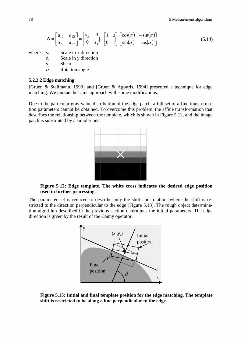
78 5 Measurement algorithms

( ) ( )( ) ( )

−⋅

⋅

=

=

αααα

cossinsincos

101

00

2221

1211 ss

saaaa

y

xA (5.14)

where sx Scale in x direction sy Scale in y direction s Shear α Rotation angle

5.2.3.2 Edge matching [Gruen & Stallmann, 1993] and [Gruen & Agouris, 1994] presented a technique for edge matching. We pursue the same approach with some modifications. Due to the particular gray value distribution of the edge patch, a full set of affine transforma-tion parameters cannot be obtained. To overcome this problem, the affine transformation that describes the relationship between the template, which is shown in Figure 5.12, and the image patch is substituted by a simpler one.

Figure 5.12: Edge template. The white cross indicates the desired edge position used in further processing.

The parameter set is reduced to describe only the shift and rotation, where the shift is re-stricted to the direction perpendicular to the edge (Figure 5.13). The rough object determina-tion algorithm described in the previous section determines the initial parameters. The edge direction is given by the result of the Canny operator.

θ

Initialposition

Finalposition

y

x

(xs,ys)

Figure 5.13: Initial and final template position for the edge matching. The template shift is restricted to be along a line perpendicular to the edge.

5.2 Algorithms used for measuring objects 79

The transformation is given by ( ) ( ) ( )

( ) ( ) ( )ααθααθ

cossinsinsincoscos

00

00

⋅+⋅+⋅+=⋅−⋅+⋅+=

yxtyyyxtxx

s

s (5.15)

where xs, ys Start position. The shift is calculated relative to this position perpendicular to the edge.

t Shift factor α Rotation angle θ Direction perpendicular to the edge

The linearized version is given as ( ) ( ) ( ) ( ) ( )( )

( )( ) ( )( )( ) ααα

θθ

dygxgygxg

dtggyxgyxeyxf

xyyx

yx

⋅−++−

+⋅⋅+⋅+=−

0000

0

cossin

sincos,,, K (5.16)

and the vector of unknowns is x = [dt, dα]T. The least squares matching solution is then obtained using the same approach as described in the previous section. This least squares edge matching yields only one object point on the boundary. But we are interested in a geometric description of the linear boundary. Thus, the edge matching is ap-plied to each edge pixel along the roughly determined line. To prevent side effects when matching at the line end (no edge pixels on either side of the template) the matching is only applied to edge pixels that are half the template size away from the line end. The eliminating of edge pixels at the line end is illustrated in Figure 5.14.

Edge Pixels

Pixels usedfor LSM

Figure 5.14: Eliminate edge pixels at line end with respect to the used template size.

Finally, the line describing the object boundary is determined by fitting a straight-line into the positions found by edge matching, cf. Figure 5.15. Based on the residuals of the fitting, out-liers can be detected and eliminated.

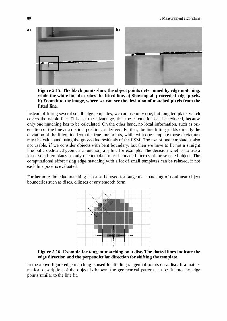
80 5 Measurement algorithms

a) b)

Figure 5.15: The black points show the object points determined by edge matching, while the white line describes the fitted line. a) Showing all proceeded edge pixels. b) Zoom into the image, where we can see the deviation of matched pixels from the fitted line.

Instead of fitting several small edge templates, we can use only one, but long template, which covers the whole line. This has the advantage, that the calculation can be reduced, because only one matching has to be calculated. On the other hand, no local information, such as ori-entation of the line at a distinct position, is derived. Further, the line fitting yields directly the deviation of the fitted line from the true line points, while with one template those deviations must be calculated using the gray-value residuals of the LSM. The use of one template is also not usable, if we consider objects with bent boundary, but then we have to fit not a straight line but a dedicated geometric function, a spline for example. The decision whether to use a lot of small templates or only one template must be made in terms of the selected object. The computational effort using edge matching with a lot of small templates can be relaxed, if not each line pixel is evaluated. Furthermore the edge matching can also be used for tangential matching of nonlinear object boundaries such as discs, ellipses or any smooth form.

Figure 5.16: Example for tangent matching on a disc. The dotted lines indicate the edge direction and the perpendicular direction for shifting the template.

In the above figure edge matching is used for finding tangential points on a disc. If a mathe-matical description of the object is known, the geometrical pattern can be fit into the edge points similar to the line fit.

5.2 Algorithms used for measuring objects 81

5.2.3.3 Disc matching The matching of a disc is needed for measuring reference markers of known size. Due to rota-tional symmetry of the disc, rotation is not estimated. The transformation is reduced to

02

001

ysbyyssxsbx

y

xx

⋅+=⋅⋅+⋅+=

(5.17)

The linearized relation between image and template with respect to the above transformation is given by ( ) ( ) ( )

( ) dssygdsygdsysxg

dbgdbgyxgyxeyxf

xxyyxx

yx

⋅⋅⋅+⋅⋅+⋅⋅+

+⋅+⋅+=−

0000

210 ,,, K

(5.18)

and the vector of unknowns is x = [db1, db2, dsx, dsy, ds]T. In the figure below, two types of disc templates are shown. a)

b)

Figure 5.17: Artificial disc template. a) Black and white template. b) Blurred ver-sion of a).

It is not necessary to use all pixels for calculating the gray values difference, especially for discs of diameter bigger than about 20 pixels. The homogenous parts, the inner of the disc and the corners of the template, don’t carry much of information and potentially contain blunders. Therefore, those parts could be explicitly excluded from the matching.

5.2.3.4 Corner matching There exist object shapes, where it is not possible to determine a corner point by matching two separate lines that intersect. If the corner is too small, edge matching in the corner region produces matching errors, because the template does not adequately correspond the reality (Figure 5.18).

82 5 Measurement algorithms

y

x

Region producingmatching error

Edgetemplate

Figure 5.18: Matching at a corner using edge template produces a localization er-ror.

Thus, we match one corner template instead of edge templates to determine the corner point, shown in Figure 5.19. Only quadratic templates are used. a)

b)

Figure 5.19: Two variations of a corner template. a) The inner part of the corner is used in the matching. b) Only the region where the edge transition occurs is used in the matching.

We can use the basic approach by applying an affine transformation as described in section 5.2.3.1 and fixing the scale in both directions to one. But this would have the drawback of scaling the length of the two sides of the corner differently. The length difference depends on the enclosed angle at the corner tip. The bigger the deviation of the angle from 90° the more is the length difference. To overcome this disadvantage, a transformation allowing to shift and to rotate the template in both directions similar to the basic approach is used, where the scale is newly applied perpendicular to the corner’s diagonal as shown in Figure 5.20 to provide a symmetrical stretching. In summing, the single transformations yield ( ) ( )

( ) ( )

++−+−+

−⋅+

=

0

0

2

1

1111

cossinsincos

5.0yx

ssss

bb

yx

dd

dd

αααα

(5.19)

where [b1, b2]T Shift vector α Rotation angle sd Scale factor perpendicular to the diagonal

The vector of unknowns is given as x = [db1, db2, dsd, dα]T.

5.2 Algorithms used for measuring objects 83

a)

b) y

x

d

d

Figure 5.20: a) Scaling of the template along the diagonal line. b) Geometric pa-rameter definition of the quadratic template.

In Figure 5.21 an example of the matching process of a corner object is shown. The initial values for the four unknown parameters are calculated from the approximate lines, because no rough boundary localization is applied.

Finalposition

Initialposition

y

x

Figure 5.21: Corner matching from initial to final position.

5.2.3.5 LSM including blur estimation [Krauth & Wrobel, 1993] describe an approach to simultaneously estimate the affine trans-formation parameter and image blur using deconvolution based on the point spread function. We want estimate the blur, which is modeled by a 2D Gaussian. There are two possibilities to determine the blur. • The relation between the image patch and the template is extended by convoluting the

basic template with a Gaussian. Thus the affine transformation parameters and σ of the Gaussian, describing the blur, are estimated simultaneously. We will call this ‘inline’ es-timation of the blur.

• In each iteration step of the LSM, σ is determined by comparing the image patch and the template. A new template is calculated by blurring the basic template with the estimated σ. This new template is used in the next iteration step of the LSM. We will call this ‘itera-tive’ estimation of the blur.

To prevent errors due to misalignment of the template and image patch, the blur is estimated after the third iteration of LSM.

84 5 Measurement algorithms

The formulas that describe the inline estimation are outlined in the following. The basic tem-plate f(x,y) is convolved with a Gaussian and the image patch g(x,y) is subtracted. Due to the symmetry of the Gaussian, the convolution can be separated in x and y. ( ) ( ) ( )yxgyxeyxf bb ,,,, =−σ (5.20)

( ) ( ) ( ) ( )∫ ∫

∞

∞−

∞

∞−

−⋅−⋅= ydyyGxdxxGyxfyxf bb ,,, σ (5.21)

where fb(x, y, σb) Template filtered with a Gaussian using σb

( ) 2

2

2

21 b

x

bexG σ

σπ

−

= Gaussian function

Through linearization, the corresponding observation equation becomes

( ) ( ) ( )

( ) ( ) ( ) dyy

yxgdxx

yxgyxg

yxedyxfyxf bb

bbbb

⋅∂

∂+⋅

∂∂

+=

−⋅∂

∂+

,,,

,,,,,

0

0 σσ

σσ

(5.22)

This can be brought to the same form as the general LSM ( ) ( ) ( ) ( ) ( )

( )b

b

bb

bb

dyxf

dyy

yxgdxx

yxgyxfyxgyxe

σσ

σ

σ

⋅∂

∂

−⋅∂

∂+⋅

∂∂

+−=−

,,

,,,,,, 00 K

(5.23)

And in matrix form: lAxe −=− ; P (5.24) The unknowns are extended by one parameter to x = [db1, db2, da11, da12, da21, da22, dσb]T. The algorithm for the iterative estimation of the blur is equivalent to the inline approach, but no affine transformation parameters are estimated. So we get the linearized form of the obser-vation equation

( ) ( ) ( ) ( )yxgyxedyxf

yxf bb

bbbb ,,

,,,,0 =−⋅

∂∂

+ σσ

σσ (5.25)

with only one unknown parameter σb to determine. The use and the benefit or drawback of this extension of the LSM is evaluated in chapter 7 by means of experiments.

5.2 Algorithms used for measuring objects 85

5.2.4 Object distance measurement The distance is the last component to measure to complete the 3D measurement. To this end, we use the reflectorless laser range finder. It is important to exactly determine the distance on the object point. But there is potential of making errors in distance measure because the laser spot on the object is finite, in the range of 15 mm × 30 mm at 100 m [Leica, 2003].

Laser Spot

Reflection fromfront surface

Reflection fromback surface

Figure 5.22: Schematic laser spot directed to the target point. Part of the laser spot is reflected from the plane behind the object plane.

Figure 5.22 schematically shows a laser spot on the corner object (Figure 5.23 a)). The laser beam is reflected from two planes different in depth. Thus, the distance measured is a combi-nation of the distance to the front and the back wall [Dzierzega, 1986; Deumlich & Staiger, 2002]. Commonly this is overcome by measuring the distance at a position slightly offset from the object to guarantee, that the full laser spot is on the same plane (Figure 5.23 b)). As we will see in chapter 7, the range finder causes the main error in IATS system. One reason for distance measurement errors is this effect of multipathing. But also the angle of incident of the laser beam influences the quality of the distance measurement. a) b) c) d)

Figure 5.23: Different methods to determine the distance to the object. a) Common approach to measure directly on the object. b) Measuring slightly offset from the object. c) Determine a plane in 3D by measuring three points on that plane. The pointing direction is intersected with the plane to get the distance. d) Line scanning towards the object point. The line is extrapolated in 3D to get the distance on the object point.

To overcome this problem, we propose an approach, where a plane is determined, given by three 3D points, Figure 5.23 c), wherein the object point lies. The pointing direction towards the object is then intersected with this plane yielding the distance and simultaneously the 3D coordinates. Figure 5.24 illustrates the procedure of intersecting the pointing direction with a plane given by three points.

86 5 Measurement algorithms

Plane

3 Points definethe plane Pointing

Direction

Figure 5.24: Intersecting the pointing direction with a plane.

The distance can be determined more precisely, while on the other hand we are faced with higher processing time, because three points are measured instead of only one. In some target situations it is not possible to determine a plane, then distance can be found by line scanning. Along a line defined by the object point and a manually set point several 3D points are measured (Figure 5.23 d)). In Figure 5.25 the principle of the line scanning is shown. At least two points have to be measured in 3D to determine the line trough the object point. The object point distance is then determined by calculating the shortest distance be-tween the scanning line and the line defined by the pointing direction. The point on the point-ing direction nearest to the scanning line defines the object distance.

Point to definethe scanning line

PointingDirection

Figure 5.25: Principle of line scanning.

These two approaches of determine a plane or a 3D line by measuring the object distance is rather cumbersome. But with the current prototype of the IATS we have no other possibility for a better solution. In future one should consider a range finder with the possibility to scan objects within the optical field of view or employ a laser beam of smaller diameter to deter-mine the distance more precisely.

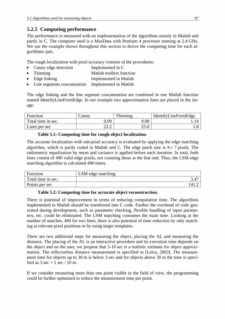
5.2 Algorithms used for measuring objects 87

5.2.5 Computing performance The performance is measured with an implementation of the algorithms mainly in Matlab and partly in C. The computer used is a MaxData with Pentium 4 processor running at 2.4 GHz. We use the example shown throughout this section to derive the computing time for each al-gorithmic part. The rough localization with pixel accuracy consists of the procedures: • Canny edge detection Implemented in C • Thinning Matlab toolbox function • Edge linking Implemented in Matlab • Line segments concatenation Implemented in Matlab The edge linking and the line segment concatenation are combined in one Matlab function named IdentifyLineFromEdge. In our example two approximation lines are placed in the im-age. Function Canny Thinning IdentifyLineFromEdge Total time in sec. 0.09 0.08 1.14Lines per sec 22.2 25.0 1.8

Table 5.1: Computing time for rough object localization. The accurate localization with sub-pixel accuracy is evaluated by applying the edge matching algorithm, which is partly coded in Matlab and C. The edge patch size is 9 × 7 pixels. The radiometric equalization by mean and variance is applied before each iteration. In total, both lines consist of 490 valid edge pixels, not counting those at the line end. Thus, the LSM edge matching algorithm is calculated 490 times. Function LSM edge matching Total time in sec. 3.47Points per sec 141.2

Table 5.2: Computing time for accurate object reconstruction. There is potential of improvement in terms of reducing computation time. The algorithms implemented in Matlab should be transferred into C code. Further the overhead of code gen-erated during development, such as parameter checking, flexible handling of input parame-ters, etc. could be eliminated. The LSM matching consumes the main time. Looking at the number of matches, 490 for two lines, there is also potential of time reduction by only match-ing at relevant pixel positions or by using larger templates. There are two additional steps for measuring the object, placing the AL and measuring the distance. The placing of the AL is an interactive procedure and its execution time depends on the object and on the user, we propose that 5-10 sec is a realistic estimate for object approxi-mation. The reflectorless distance measurement is specified in [Leica, 2003]. The measure-ment time for objects up to 30 m is below 3 sec and for objects above 30 m the time is speci-fied as 3 sec + 1 sec / 10 m. If we consider measuring more than one point visible in the field of view, the programming could be further optimized to reduce the measurement time per point.

88 5 Measurement algorithms

5.3 Algorithms for selected objects Based on the algorithms defined in the previous section a wide variety of different objects can be determined in 3D space. In this section we introduce a collection of objects, which we use for benchmarking. Measuring an object line in the image is a basic operation to determine different objects in 3D. This procedure, we call it ‘line-measuring’, works as follows: • The user places an approximate line (cf. section 5.2.1). • Valid edge pixels representing an object boundary are determined using the rough object

localization algorithm consisting of edge detection followed by line segment concatena-tion (cf. section 5.2.2).

• Apply edge matching to determine the exact local boundary position and finally fit a straight line into those boundary pixels (cf. section 5.2.3.2)

This algorithm yields an object position in the image with sub-pixels accuracy.

5.3.1 Disc measurement for reference benchmark We use circular targets to benchmark the measurement accuracy. We describe two possibili-ties to determine a disc, given by its center and radius. • Determine the disc by LSM using an artificial disc template. • Determine the disc by matching multiple edge segments (tangents) at the disc boundary

and fit an ellipse. The rough disc position in the image can be found by manually placing a circle or by normal-ized fast cross-correlation. In the latter case, the diameter of the disc in the image must be roughly known to build a template. The diameter of the disc can be determined by using the focus lens position to estimate the magnification. Based on the diameter we build the template for LSM disc matching and the disc matching delivers the disc center and the scaling to calculate the precise diameter. An edge template is used to find positions of the disc boundary. The template size for the tan-gent matching should be in the order of 9 × 9 pixel (depending on the magnification) because of discrepancy between the straight edge line and the bent disc border. Multiple tangent matching all over the disc is calculated. The start parameters for the tangent matching must be calculated relative to the disc center using the diameter. Finally, if multiple boundary points are identified, an ellipse fit is calculated to find the real center and diameter of the disc. The distance of the disc target is measured exactly in the disc center.

5.3.2 Measurement of objects defined by intersection of two lines Many types of object points are defined by two intersecting lines, e.g. house edges, window frames corners, door corners, etc. An object point defined by the intersection of two lines is determined using the following al-gorithm: • Apply the line-measuring algorithm for two lines that intersect at the desired object point • Intersect the two resulting lines and calculate the position in the image • Use the back-transformation algorithm to determine the horizontal and vertical angles of

the object point

5.3 Algorithms for selected objects 89

• Finally measure the distance to the point using any of the four approaches, described in section 5.2.4.

5.3.3 Measurement of a pole Measuring a cylinder (e.g. pole, tube or pillar) could be used for example in hidden point ap-plications using a pole of defined length or in measuring heating tubes etc. There, the coaxial vector and the radius of the cylinder are the desired parameters.

Cylinderboundary

Centerline

Figure 5.26: Example of measuring the boundary lines of a heating tube.

With the line-measuring algorithm the boundary of the cylinder in the image is determined. Then the bisecting or center line of both boundaries is calculated as illustrated in Figure 5.26. Measuring the distances of multiple points on the bisecting line yields 3D points on the cylin-der surface. Those points define the pointing direction of the coaxial vector. The pivot point of this vector is calculated by shifting a point on the bisecting line in pointing direction per-pendicular to the 3D bisecting line by the radius. The radius is calculated based on the distance between the boundary lines. But due to the im-aging, this distance represents not the real diameter as shown in Figure 5.27.

ImageSensor

Distance dγ

Cylinder

rr'

Figure 5.27: Principle of imaging a cylinder on the image plane.

The radius can be calculated easily using the equation ( )

( ) dr ⋅−

=γ

γsin1

sin (5.26)

Where

r Radius of the cylinder d Object distance γ Half the angle between the cylinder boundaries

The coaxial vector and the radius define the cylinder in 3D space.

90 5 Measurement algorithms

5.3.4 Measurement of objects defined by tangents Objects that cannot be described by linear boundaries are determined by matching tangents as described in section 5.2.3.2 using edge matching. The user therefore specifies manually points to be measured. Edge points, determined by the Canny detector, closest to the approximate points define the start parameter for the edge matching. The result of all matching yields sev-eral local boundary points of the object. To measure the distance, there exist two different methods. Either a plane is defined by measuring at least three 3D points wherein all those tangent points lie or for each point the distance is measured. Single distance measurements can be applied directly on the object point or at a predefined position. To get a 3D representa-tion of the object, a geometric model must be available.

5.3.5 Measurement of a prism plate Because the ATR (automatic object recognition) is not installed in the prototype of the IATS it is not possible to measure automatically on prisms shown in Figure 5.28 a). Such a prism is used to set up a theodolite station using known points or for measuring new ground points. Thus, an algorithm is developed to measure this type of prism using the white or yellow trian-gles on the plate around the prism. The corner points of the triangles in the image are determined using the line-measuring algo-rithm. The center of the prism is in the middle of the connection line of the two side triangles. Further, the plumb line of the upper triangle corner to the horizontal connection line should intersect at the same position, Figure 5.28 b). The average of those two positions is taken as prism center for further processing. If the deviation between those two points exceeds a cer-tain limit, then the measurement is discarded. a)

b)

PrismCenter

MatchedLines

MatchedLines

Figure 5.28: a) Prism used for measuring with traditional theodolite. b) Using the measurement algorithm two-line-intersection to determine the corner points of the three triangles and thereof the center of the prism.

The distance of the prism is measured directly in the prism center. Instead of the reflectorless range finder, the conventional range finder for prism installed in IATS must be used. This is an example on how easily the basic algorithms can be extended to measure complex objects. Instead of placing three polylines for each triangle, a pattern consisting of all triangles can be placed. Thus, using only one template decreases the execution time and makes the ob-ject approximation more comfortable for the user, because only one approximation template must be placed instead of 6 approximation lines.

5.4 Conclusions of the chapter 91

5.4 Conclusions of the chapter We have developed algorithms based on geometric primitives to measure complex objects in the 3D space using image processing and matching techniques simultaneously with a laser range finder for reflectors and reflectorless. Those algorithms can easily be extended to dif-ferent other objects by combining the particular approaches. Further developments should address the robustness. To prevent measurements on dynamic objects, a check based on image differencing could be applied. Various approaches for detec-tion of blunders are described in [Pateraki, 2000]. The potential and practical use of those algorithms will be shown in a benchmarking section.

6 Calibration The Image Assisted Total Station must be calibrated as any other theodolite. But since no visual path for direct observation is available, a new concept must be defined including the new sensors like the CCD-camera and the focus encoder. The following procedure has been chosen: First, the line of sight stability over temperature is inspected. This delivers angular correction terms. After it we measure the camera constant as function of all opto-mechanical parameters involved and finally the mapping parameter and the theodolite axis corrections are calibrated. There exist many approaches to estimate the parameters. A widely used one is a least squares estimation routine described in [Höpcke, 1980; Strang & Borre, 1997; Koch, 1999]. The ob-servation equations must be linear in terms of the unknown variables. In the following we will use a Maximum-Likelihood estimator, cf. [Stuart, Ord & Arnold, 1999].

6.1 Line of sight stability over temperature Traditional theodolites are calibrated within the specified temperature range. The instrument’s axes errors, vertical-index error and collimation error dependence is then expressed by coeffi-cients [Zeiske, 2000].

6.1.1 Framework of the temperature dependent correction Since the vertical-index error and the collimation error depend on the temperature, we will correct the formulas for the horizontal and vertical angles defined in section 4.2 by adding a temperature dependent term. Vertical angle corrected by the vertical-index error

Temp,1DeviceRef,1, eteVV TCT ⋅∆−−= (6.1)

where VT,C Vertical angle corrected by the vertical-index error VT Measured vertical angle (raw angle) e1,Ref Vertical-index error at reference temperature e1,Temp Temperature coefficient of the vertical-index error ∆tDevice Temperature difference (Instrument temperature) relative to

20°C

94 6 Calibration

Horizontal angle corrected by collimation and tilting axis error

( )CTTCT V

eteHzHz

,

3

CT,

Temp2,DeviceRef,2, tan)sin(V

e+

⋅∆+−= (6.2)

where HzT,C Horizontal angle corrected by the collimation and the tilting axis error

HzT Measured horizontal angle (raw angle) VT,C Vertical angle fully corrected e2,Ref Collimation error at reference temperature e2,Temp Temperature coefficient of the collimation error e3 Tilting-axis error (not depending on temperature) ∆tDevice Temperature difference (Instrument temperature) relative to

20°C The objective of the line of sight stability calibration is to determine the parameters e1,Ref, e1,Temp, e2,Ref and e2,Temp. The vertical-index and the collimation error at reference temperature could also be determined by the axis calibration procedure described in section 6.3.

6.1.2 Calibration procedure The calibration procedure to determine the axis error correction coefficients at different tem-peratures is outlined in the following. The theodolite is placed on a pole in a temperature chamber as shown in Figure 6.1.

Figure 6.1: Theodolite in temperature chamber mounted on a pole.

The theodolite is focused on a collimator, which is placed behind the circular window left in the figure. The reticle of the collimator is used as target to determine both axis errors. The mapping parameters of the inner orientation (affine transformation without shift) are not known. Thus they are set to initial values sx = 1 Scale in x sy = 1 Scale in y s = 0 Shear α = 0 Rotation

6.1 Line of sight stability over temperature 95

This is a valid assumption, because the theodolite positions itself iteratively until the crosshair matches with the target within ± 1 pixel. Therefore the errors based on the parameters of the inner orientation are negligibly small. The collimation error and the vertical-index error are determined by measuring the polar an-gles of the center of the collimator crosshair in both faces. The related calculations are de-scribed in section 4.2. To measure the pointing direction of the target, its image position is found by LSM and the back-transformation algorithm is applied to get the polar angles. An image patch of the initial image of the crosshair will be used as template for LSM to deter-mine the actual crosshair position relative to the initial one. This template is used throughout the calibration process. The measurement in both faces is performed rather quickly so we have not to expect any thermal deformation of the environment. The axis errors are determined first at temperature +20°C, then at -20°C and at +50°C and finally again at 20°C. There was enough time between the measurements that the theodolite reached a thermal stationary state. We expect a hystersis error, i.e. the difference of the axis errors at the initial and final meas-urement at 20°C, below 3 mgon. Experience with traditional theodolites shows that the hys-teresis error normally is in the order of 1-2 mgon.

6.1.3 Calibration results Several calibration runs were performed and the results are summarized below.

Figure 6.2: Temperature dependent collimation and vertical-index error.

Figure 6.2 shows the collimation and vertical-index error relative to the first measurement at 20°C. The dotted gray line is the regression line. The hysteresis error is found as

Collimation error: -0.5 mgonVertical-index error: -0.6 mgon

Table 6.1: Hysteresis error. The slope of the regression line corresponds to the temperature dependent coefficients e1,Temp and e2,Temp, while the mean of the measurement at 20°C yields the correction coefficients e1,Ref and e2,Ref.

96 6 Calibration

Temperature coefficient of Collimation error (e2,Temp): -1.593e-007 rad / °C -0.01 mgon / °CVertical-index error (e1,Temp): 2.113e-006 rad / °C 0.14 mgon / °C

Table 6.2: Temperature coefficients for collimation and vertical-index error. The results show that the collimation error is insensitive to temperature changes. Even tem-perature differences of 20°C cause only a change of 0.2 mgon, which is below the measure-ment accuracy of the instrument. But the influence on the vertical-index error is significantly higher. A temperature change of only 3°C causes a change of 0.5 mgon, which is in the range of the angle measurement accuracy.

6.2 Camera constant As described in section 4.1.2, the camera constant c is calculated in terms of the encoder posi-tion p, the encoder origin position OL, the gradient SL of the encoder gear and the distance LS between the rear principal plane of the front lens and the image sensor. Further, the object distance is calculated using these four parameters and additionally the distance doffset between the front vertex of the main lens and the standing axis. The parameters SL and doffset are well known from the mechanical specifications and should be confirmed within the required accu-racy by the calibration routine. The other parameters are approximately known from the me-chanical specifications. An obvious approach to determine the camera constant would be to use the magnification of the optics for the actual lens position. But in praxis it is not possible to determine the magnifi-cation directly, because the object is not known a priori. Thus, the only possibility to derive the camera constant is the use of the encoder position, which describes the optical system. Therefore, we are forced to calibrate the encoder in relation to the opto-mechanical parame-ters to be able to derive the correct camera constant for each focus lens position. During the calibration we will make use of the magnification, because the dimension of the target used are known.

6.2.1 Calibration for any focus position To determine the optics and mechanics parameters we use the relation between those parame-ters and the object distance and the optical magnification. The distance and the magnification can be measured for a known object using the range finder and LSM, while simultaneously the encoder position at the best focus position is measured. Using these measurements and the relations, an estimation problem is formulated that has to be solved. Field measurements were done, measuring the object distance, the best focus lens position and the optical magnification. The object is placed at different distances. For each object setup the best focus position is calculated using different contrast measurements. The object distance is measured using the reflectorless range finder and the magnification is found from the ratio of the real and the imaged diameter of the disc target as shown in Figure 6.3. The target consists of two discs on each side with diameter 15 mm and 150 mm, respectively. The diameter in the image is determined by matching an artificial disc template using LSM.

6.2 Camera constant 97

Figure 6.3: Target with disc of diameter 150 mm at a distance of 34 m.

The discs are printed on a laser printer and fixed between two glass plates. The radial devia-tion from a disc is smaller than 0.1 mm. Figure 6.4 shows the measured parameters from two measurement series. The encoder posi-tion and the magnification only change significantly below 50 m, for larger distances the changes are almost not detectable.

Figure 6.4: Results of the measurement series; Encoder position and magnification at different distances.

The different autofocus algorithms yield a repeatability of the focus lens positioning of ap-proximately ±13 steps with a standard deviation of 10 steps (1 step = 0.92 µm). Using the formulas defined in section 4.1.1 we can derive the mathematical model used in the estimation. ( )

( )SLL

offsetSLLd

LSOpf

dLSOpfd

,,;

,,,;

ββ =

=

(6.3)

98 6 Calibration

where pd ,, β The true values of the observations Npd ℜ∈,, β d Object distance relative to the standing axis [mm] β Magnification p Encoder position [steps] OL Offset of the encoder origin [steps] SL Gradient of the focus motor gear [steps/mm] LS Distance between image sensor and front lens [mm] doffset Distance between the standing axis and the front vertex of the

main lens [mm] Because the true values p of the encoder position are not known, they are treated as un-known variables in the estimation. Thus the vector of unknowns is given by: [ ] KNT

offsetSLL dLSO +ℜ∈= ;;;;px (6.4)

The stochastic model is given by dvdd += ( )dd Nv σ,0~

βββ v+= ( )ββ σ,0~ Nv

pvpp += ( )pp Nv σ,0~ (6.5)

The standard deviations of the observed values are derived from measurements. The joint probability density function under the above assumption is:

( )( )

++−

⋅

⋅⋅⋅

=2

2

22

2

22

22

21

23

2

1,,p

p

d

d vvv

N

pd

pd evvvDσσσ

β

ββ

β

σσσπ

(6.6)

The unknowns have to be determined by maximizing the function D(νd, νβ, νp). This is equivalent with the minimization of –log(D(νd, νβ, νp)), respectively with minimizing of

( )

( )

( )2

22

2

2

2

2

2

2

2

2

22

2

22

22

2

,,;

,,,;

,,

p

SLL

d

offsetSLLd

p

p

d

dpd

ppLSOpf

ddLSOpf

vvvvvvD

σσ

β

σ

σσσ

β

β

β

ββ

−+

−

+−

=

++=

K (6.7)

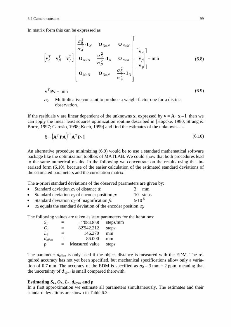
6.2 Camera constant 99

In matrix form this can be expressed as

[ ] min

2

20

2

20

2

20

=

⋅

⋅

⋅

⋅

⋅

××

××

××

p

d

Np

NNNN

NNNNN

NNNNNd

Tp

TTd

vvv

IOO

OIO

OOI

vvv ββ

β

σσ

σσ

σσ

(6.8)

min=PvvT (6.9)

σ0 Multiplicative constant to produce a weight factor one for a distinct observation.

If the residuals v are linear dependent of the unknowns x, expressed by v = A ⋅ x – l, then we can apply the linear least squares optimization routine described in [Höpcke, 1980; Strang & Borre, 1997; Carosio, 1998; Koch, 1999] and find the estimates of the unknowns as ( ) lPAPAAx ⋅=

− TT 1ˆ (6.10)

An alternative procedure minimizing (6.9) would be to use a standard mathematical software package like the optimization toolbox of MATLAB. We could show that both procedures lead to the same numerical results. In the following we concentrate on the results using the lin-earized form (6.10), because of the easier calculation of the estimated standard deviations of the estimated parameters and the correlation matrix. The a-priori standard deviations of the observed parameters are given by: • Standard deviation σd of distance d: 3 mm • Standard deviation σp of encoder position p: 10 steps • Standard deviation σβ of magnification β: 5⋅10-5 • σ0 equals the standard deviation of the encoder position σp The following values are taken as start parameters for the iterations: SL = −1'084.858 steps/mm OL = 82'942.212 steps LS = 146.370 mm doffset = 86.000 mm p = Measured value steps The parameter doffset is only used if the object distance is measured with the EDM. The re-quired accuracy has not yet been specified, but mechanical specifications allow only a varia-tion of 0.7 mm. The accuracy of the EDM is specified as σd = 3 mm + 2 ppm, meaning that the uncertainty of doffset is small compared therewith. Estimating SL, OL, LS, doffset and p In a first approximation we estimate all parameters simultaneously. The estimates and their standard deviations are shown in Table 6.3.

100 6 Calibration

Estimated parameter Estimated standard deviations

LS = −1'097.954 steps/mm LSσ = 10.443 steps/mm

LO = 8'3926.532 steps LOσ = 697.717 steps

SL = 146.444 mm SLσ = 0.291 mm

offsetd = 31.922 mm offsetdσ = 27.296 mm

pσ = 20.329 steps

Table 6.3: Results estimating all parameters. Compared with the required accuracy from section 4.4.1, all estimated standard deviations besides that of the encoder position are about a factor 12-16 too big. The absolute values of the correlation coefficients of the single parameters are shown in Figure 6.5. The assignment of the index to the parameters can be found in the list below. Parameter SL OL LS doffset p Index i 1 2 3 4 5, ..., 21

Figure 6.5: Correlation coefficients estimating all parameters.

We note a high correlation between the parameters SL and OL (0.99, variables 1 and 2) and between the parameters LS und doffset (0.93, variables 3 and 4). This is explainable by the me-chanical relation of SL and OL, and since the screen distance LS and the offset of the vertical axis from the front lens doffset are geometrically coupled. The variation of the image distance directly influences the object distance, whereof doffset is a part. Further the correlation value of the encoder positions converges to one with decreasing encoder position or equivalently with increasing distance. The reason is the small change of the encoder position at larger distances. Because the parameter doffset is known from the specification with an accuracy of

offsetdσ = 0.7 mm, which is sufficient, this parameter is fixed to 86 mm. Then the remaining

parameters are re-estimated.

6.2 Camera constant 101

Estimating SL, OL, LS, and p New estimation results, where the parameter doffset is set to a fixed value of 86.0 mm.

Estimated parameter Estimated standard deviations

LS = −1'079.342 steps/mm LSσ = 4.722 steps/mm

LO = 82'719.023 steps LOσ = 354.223 steps

SL = 145.909 mm SLσ = 0.110 mm

pσ 21.278 steps

Table 6.4: Results for estimating parameters SL, OL, LS, and p. The results are slightly better than in the previous estimation, but still not sufficient. Besides the standard deviation of the encoder position, a factor 6 is missing in the accuracy. Parameter SL OL LS p i 1 2 3 4, ..., 20

Figure 6.6: Correlation coefficients estimating parameters SL, OL, LS, and p.

The correlation between SL and OL remains high, because nothing changed between those two parameters. But the correlation between SL and LS and between OL and LS could be reduced. Estimating OL, LS and p To improve the standard deviation of the estimated parameters, SL is set to the value given by the mechanical specification (−1084.858 steps/mm).

Estimated parameter Estimated standard deviations

LO = 83'129.067 steps LOσ = 47.201 steps

SL = 145.958 mm SLσ = 0.102 mm

pσ = 21.398 steps

Table 6.5: Results for estimating parameters OL, LS and p.

102 6 Calibration

Now both parameters OL and p fulfill the requirements. SLσ , however, is still a factor 5 too

big also confirmed by the correlation coefficients (Figure 6.7). The correlation between OL and LS is almost one. The geometrical configuration can be taken as reason for this. We can-not take the estimated parameters, because their estimated standard deviation is larger than the requirements. Parameter OL LS p i 1 2 3, ..., 19

Figure 6.7: Correlation coefficients estimating parameters OL, LS and p.

The correlation chart looks similar to the results of the previous evaluations. Conclusions The evaluation has shown that the estimated parameters are highly correlated and that the estimated standard deviation is high compared with the requirements. This points to a bad conditioning of the configuration. The estimated standard deviation of the single parameters could be improved by setting those parameters to the fixed value known from the mechanical specifications. But the results are still not within the requirements. Thus, we can conclude that the above approach for calibrating the optical and mechanical parameters is not successful and we have to find another way to determine the camera constant for the actual focus lens posi-tion. First choice to determine the camera constant is to use an online camera constant calibration procedure, where the camera constant is determined for each new focus position during the measurement. This approach is described in the next section and we will use it to during the benchmarking. To omit the online calibration, the design of the opto-mechanical system should be reconsid-ered. A further possibility would be to define a calibration procedure for each individual pa-rameter independent from the others. This requires new measurement procedures and new calibration equipment. Before implementation in products this approach must be reconsid-ered.

6.2 Camera constant 103

It is possible to measure the camera constant actively using a laser diode. The laser is imaged through the optical system onto the image sensor. The angle ϕ of the laser beam relative to the plane orthogonal to the optical axis is determined by a calibration procedure. With this con-figuration the laser beam simulates an incoming ray of an object under the viewing angle ϕ. By measuring the position yI of the laser spot on the image sensor it is possible to calculate the camera constant.

( )ϕtanIy

c = (6.11)

This measurement procedure is applied whenever the focus lens has moved.

MathematicalImageSensor

c

yI

Laser Diode

ENP

ϕ

ϕ

ϕ

MirrorOptical Axis

Figure 6.8: Imaging of a laser beam of known angle of incident through the optical system on the sensor for an arbitrary focus lens position.

6.2.2 Online calibration of single focus position The goal of this calibration routine is to determine online the camera constant for the actual focus lens position during a survey.

c

Object Q

Image Sensor(Position 2)

Pointing Axis(Position 1)

Pointing Axis(Position 2)

Image Sensor(Position 1)

ϕ

∆r

ENP

q1q2

q1

Figure 6.9: Imaging configuration for online camera constant calibration.

In chapter 4 the relation between the theodolite pointing direction, the object polar angles and the object position on the sensor is derived. This relation is used to determine the camera con-stant. The same object is measured at different pointing directions of the theodolite as shown

104 6 Calibration

in Figure 6.9. For each pointing direction, the theodolite horizontal and vertical angles and the target position on the image sensor q1 and q2 are registered. The unknown parameters are the camera constant c and the polar angles HzQ and VQ of the object. These parameters are deter-mined using a least squares. In this estimation the mapping parameter must be known. Be-cause there are 3 unknown parameters, at least two pointing directions of the theodolite are needed to solve the estimation problem. The target position is determined by LSM. Therefore, an image patch containing the object is selected as template. The pointing directions are selected to cover maximal range of the an-gles.

6.3 Mapping parameter and theodolite axis error There are several possibilities to calibrate the mapping parameters described by the inner and outer orientation. For the calibration of the inner orientation parameters one can take a 2D or 3D target [Luhmann, 2000], also often used for the camera calibration in photogrammetry [Bayer, 1987; Bayer, 1992; Gruen & Huang, 2001]. Another possibility is based on scanning a fixed target with the theodolite [Huang & Harley, 1989]. The theodolite axis errors (vertical-index, collimation and tilting axis error) are determined by two-face measurements of several objects [Deumlich & Staiger, 2002; Dzierzega & Scherrer, 2003]. The difference between the angles measured in both faces defines the axis errors.

6.3.1 Photogrammetric camera calibration approach The camera calibration is performed using a 2-dimensional target. The target consists of 48 white discs on black background. The discs are arranged on an orthogonal grid as shown in Figure 6.10. The diameter of each disc is 8 mm and the distance between the disc centers is 20 mm. The numbering of the discs is from left to right and from top to bottom. The disc No. 37 is missing for unique target orientation, but it is also counted. a)

b)

1 7

43 49

20 mm

20 mm

8 mm

Figure 6.10: a) Image of the gimbals-mounted 2D target. b) Schematic description of the 2D target.

The target could be rotated around all three axes due to its gimbals-mounting, allowing to keep the theodolite (camera) fixed (Figure 6.11). The distance between the target and the theodolite is 15 m. Eight images of the target at different viewing angles were recorded. The starting values for the parameter estimation are derived from the theodolite distance meas-

6.3 Mapping parameter and theodolite axis error 105

urement and the angle readings of the target mount. The field of view of the camera at 15 m equals 1.4 (Hz) × 1.1 (V) gon. Compared with photogrammetric camera the field of view is extreme small.

X

Z

ω'

ϕ'

κ'

Y

Theodolite

Target

Figure 6.11: Setup of theodolite and 2D target for image recording.

We try to determine the parameters of the inner and outer orientation with the help of the software SGAP [Mason, 1994]. Unfortunately, the software was not able to determine esti-mates for the camera constant and the principal point. The program SGAP terminated estima-tion process with a failure, indicating a singular matrix. It was not able to solve the estimation problem due to numerical computation problems. The same problem occurred if the addi-tional parameters describing the optical distortion [Brown, 1971] are estimated. Further, we try to estimate the theodolite station coordinates, while all parameters of the inner orientations are fixed. This results in a estimated precision of the station coordinates of 33.9 mm in X, 34.1 mm in Y and 4.0 mm in Z direction, which is not to be used further. If the geometrical configuration of imaging the target onto the sensor is inspected, it becomes apparent why the stations cannot be estimated accurately. In Figure 6.12 the relations are shown. The images a and b of the target points A and B are compared with the image points a′′ and b′′ after shifting orthogonal to the pointing axis and rotating the target, where the en-trance pupil is the rotation center. The transformation (shift and rotation) is calculated such that the image of A resides at the original position. All points on the optical axis change their position on the image sensor.

ENP

Sensor

Target

A

A'

B'

A''

B'' B

b''

b∆yb

ϕ

a=a''

Figure 6.12: Image of a target after shifting and rotating.

106 6 Calibration

The difference between the image points is given by:

+⋅+−⋅⋅=∆ 22

1tytd

dd

ycyB

Bb (6.12)

where yB Distance of the point B from the pointing axis d Target distance from the entrance pupil c Camera constant t Shift orthogonal to the pointing axis Further the assumption is made, that the field of view is small and there-fore the following simplifications were made:

( )( )( ) 1cos

sintan

===

ϕϕϕϕϕ

We chose the rotation and the shift in a way, that the image of the object A is invariant in its position. This means, the object point A on the optical axis is transformed to the point A′′, which again is on the optical axis.

The angle ϕ is defined by ( )dt

=ϕtan .

If we use the results from the SGAP estimation, where the lateral uncertainty of the station is approximately 34 mm we get the following result for the image displacement: Camera constant: c = 228 mm Position in the image yB = 197 mm Distance d = 14.96 m Orthogonal shift t = 34 mm Rotation angle ϕ 0.15 gon Uncertainty in the image position ∆ yb = 0.11 µm From the calculation above we can conclude, that a shift of 34 mm of the object (or the sta-tion) can be compensated by a rotation of 0.15 gon resulting in a shift below 0.1 µm in the image. Keeping in mind, that the LSM yields localization resolution in the order of one tenth of a pixel (0.6−0.9 µm) in real environments, it is not possible to distinguish between shift and rotation of the said size. This is a result of the small angle differences between the ob-jects. The small field of view does not allow measuring objects where the angle difference is larger. Thus, this approach could not be used to determine the inner orientation of the camera system.

6.3.2 Scanning calibration approach As described in the previous section, it is not possible to use standard routines and targets from photogrammetry for calibrating the inner and outer orientation. Therefore a new calibra-tion concept is worked out and called ‘Theodolite-Sensor-Calibration’ (TSC). According to the results of the previous section we model the inner orientation as linear function and apply the affine transformation without shift not considering optical distortion as outlined in sec-tion 4.3.1.

6.3 Mapping parameter and theodolite axis error 107

We will measure an object from several pointing directions as shown in Figure 6.13 in both telescope faces. The scanning is done grid wise that the image of the object moves on the im-age sensor. For each direction the theodolite angles (horizontal and vertical) are measured and using LSM derives the object location on the sensor.

Hz

V

Hz Range

V R

ange

V

Figure 6.13: Scanning of an object with the total station.

To lower the correlation between the parameters of the inner orientation and the theodolite axis errors, several objects at different elevations are preferable for the scanning. The goal of the calibration is to deliver the following parameters A Parameter of the affine transformation without shift, also described by sx, sy, s, α e1 Theodolite vertical-index error e2 Theodolite collimation error e3 Theodolite tilting axis error Since both polar angles HzQ(i) and VQ(i) of the object i are unknown, they will be included in the estimation. We use the same estimation framework as described in the estimation process of the optics-mechanics parameters for the camera constant in section 6.2.1. The functional model is based on the mapping relations between sensor space and object space expressed by the following formulas (4.41) and (4.42) ( ) ( )

( ) ( )QQyxTTyTA

q

QQyxTTxTA

q

VHzeeesssVHzfy

VHzeeesssVHzfx

,,,,,,,,,,

,,,,,,,,,,

321

321

α

α

=

=

′

′ (6.13)

108 6 Calibration

where ( ) ( )TT

TAq

TAq VHzyx ,,, ′′ are the true values of the observations ( ) ( ) N

TTTA

qTA

q VHzyx ℜ∈′′ ,,,

Parameters:

( ) ( )TAq

TAq yx ′′ , Position of the object in the image relative to the cross-

hair position [mm] HzT, VT Measured theodolite horizontal and vertical angles (raw

angle, without any corrections) sx, sy, s, α Affine transformation parameter. For each target a scal-

ing factor in x and y direction is determined, while only one shear and one rotation angle for all measurement.

e1, e2, e3 Theodolite axis corrections HzQ, VQ Object polar angles

The values THz and TV describing the true theodolite polar angles are included in the vector of unknowns: [ ] KNT

QQyxTT VHzeeesssV,Hz +ℜ∈= 2321 ,,,,,,,,, αx (6.14)

The stochastic model is given by ( ) ( )

xTA

qTA

q vxx += ′′ ( )xyx Nv σ,0~ ( ) ( )

yTA

qTA

q vyy += ′′ ( )xyy Nv σ,0~

HzTT vHzHz += ( )AngHz Nv σ,0~

VTT vVV += ( )AngV Nv σ,0~

(6.15)

The standard deviations of the observed values are assumed to be known. The joint probabil-ity density function under the above assumption is: ( )

( )( )

+

++

−

⋅⋅⋅

=

2

22

22

2

2

222

21

22222

1

,,,

Ang

VHz

xy

yx vvvv

NAngxy

VHzyx

e

vvvvD

σσ

σσπ

K

(6.16)

The unknowns should maximize function D(νx, νy, νHz, νV) or equivalently minimize -log(D(νx, νy, νHz, νV)), respectively of

( ) 2

22

22

2

2

222

2 ,,,Ang

VHz

xy

yxVHzyx

vvvvvvvvD

σσ

++

+= (6.17)

In matrix form this can be expressed as

6.3 Mapping parameter and theodolite axis error 109

min

2

20

2

20

2

20

2

20

=

⋅

⋅

⋅

⋅

⋅

×××

×××

×××

×××

V

Hz

y

x

NAng

NNNNNN

NNNAng

NNNN

NNNNNxy

NN

NNNNNNNxy

T

V

Hz

y

x

vvvv

IOOO

OIOO

OOIO

OOOI

vvvv

σσ

σσ

σσ

σσ

(6.18)

min=PvvT (6.19)

We proceed in the same way as described in section 6.2.1. lxAv −⋅= (6.20)

( ) lPAPAAx ⋅=− TT 1

ˆ (6.21)

where A Design matrix P Weighting matrix

The a priori standard deviations of the observed parameters are obtained as: • Standard deviation σxy of the object position in the image 0.1 µm • Standard deviation σAng of the theodolite angle measurement: 0.3 mgon • σ0 equals the standard deviation of the object localization in the image σxy The rather complex design matrix is shown below:

Pos 1

Pos N

Target M

Target 1 Pos 1

Pos N

Pos 1

Pos N

Target 1

Pos 1

Pos N

Target 1

xq'(TA)

HzT

VT

Pos 1

Pos N

Pos 1

Pos N

Target 1

Target M

yq'(TA)

Pos 1

Pos N

Target M

Pos 1

Pos N

Target M

sx,1 sx,M... sy,1 sy,M... s a ... ... e1 e21 e22HzQ,1 HzQ,MVQ,1 VQ,MHzT,11... ... ... ... ... ...HzT,1N HzT,M1 HzT,MN VT,11 VT,1N VT,M1 VT,MN

0 1 Derivative Figure 6.14: Design-matrix structure.

110 6 Calibration

To verify the approach, a special measurement series to determine simultaneously the theodolite axis errors and the inner orientation and axis errors (TSC) is performed. We used a measurement setup (Figure 6.15) with a vertical collimator bench, where the illuminated crosshairs on the collimator reticles are the targets to aim at.

Figure 6.15: Setup for scanning calibration using vertical collimator bench.

Measurement for the axis calibration First, each target is aimed once to save the pointing direction and an image of the collimator crosshair of size 51 × 51 pixels us saved to use later as a template in the least squares match-ing (Figure 6.16). During the measurement the targets are aimed automatically in both faces applying LSM. The theodolite iteratively repositions itself until the crosshair matches the ob-ject within an accuracy of 1 pixel. Therefore, any effects of caused by the parameters of the inner orientation can be neglected. Finally the polar angles of the object are calculated using the back-transformation algorithm.

Figure 6.16: Template; Image of the collimator crosshair.

The theodolite angles are measured without any axis correction. 7 collimators are taken for the measurement, where each is aimed 5 times in both telescope faces. Calibration value Standard deviation Vertical-index error e1 1.021 mgon 0.081 mgon Collimation error e2 0.591 mgon 0.025 mgon Tilting axis error e3 -1.580 mgon 0.043 mgon

Table 6.6: Results of the theodolite axis error calibration. The results are compared later with the results of the TSC.

6.3 Mapping parameter and theodolite axis error 111

Measurement for the TSC The same targets and templates are used as in the axis error calibration above. The objects are scanned on a 7 × 7 grid in both faces as shown in Figure 6.13. Each target is scanned twice. In the table below, different configurations for the dataset used in the estimation are listed. This should show, how many targets and scanning points are necessary to provide accurate results.

A priori standard deviation of Evaluation Number

Number of targets

Number of scans of each target

Scanning grid Pixel position

[mm] Theodolite angles [mgon]

1 7 2 7 × 7 0.001 0.3 2 4 1 7 × 7 0.001 0.3 3 4 1 3 × 3 0.001 0.3 4 3 1 3 × 3 0.001 0.3 5 2 1 3 × 3 0.001 0.3

Table 6.7: Different datasets used for evaluation. The two tables below show the results of the estimation, the estimated parameters and the estimated standard deviations. Eval. sx sy s α e1 e2 e3 No. [1] [1] [1] [gon] [mgon] [mgon] [mgon] 1 0.99560 0.99604 1.34e-4 0.499 1.039 0.563 -1.7672 0.99559 0.99604 1.30e-4 0.500 1.031 0.580 -1.8233 0.99559 0.99622 1.18e-4 0.501 1.039 0.618 -1.7944 0.99558 0.99624 8.10e-5 0.499 1.019 0.624 -1.8005 0.99576 0.99621 1.12e-4 0.502 1.022 0.571 -1.832

Table 6.8: Estimated parameters for each evaluation. Eval.

xsσ ysσ sσ ασ

1ˆ eσ

2ˆeσ

3ˆeσ

QHzσ QVσ

No. [1] [1] [1] [mgon] [mgon] [mgon] [mgon] [mgon] [mgon] 1 6.29e-5 8.36e-5 3.89e-5 1.63 0.008 0.009 0.017 0.024 0.0222 6.47e-5 8.69e-5 5.32e-5 2.24 0.011 0.012 0.021 0.026 0.0233 1.44e-4 1.93e-4 1.18e-4 4.98 0.031 0.032 0.058 0.070 0.0624 1.50e-4 2.03e-4 1.43e-4 6.03 0.038 0.036 0.062 0.075 0.0655 1.45e-4 2.05e-4 1.73e-4 7.48 0.047 0.044 0.065 0.080 0.066

Table 6.9: Estimated standard deviations of the TSC optimization. The estimated standard deviation of the shear is in the same order as the estimated value. The standard deviation of the shear is small, its influence is below 0.04 pixels for an object posi-tion at the sensor border and thus it will neglected it. All other parameters are in the expected range. We note a high correlation between the shear s and the rotation α (Parameters 9 and 10, ρs,α = 0.66) and between the collimation error e2 and the tilting-axis error e3 (Parameters 21 and 21,

32 ,eeρ = 0.47) as shown in Figure 6.17, where the absolute correlation coefficients are displayed. As stated above, the influence of the shear is neglected due to its smallness and thus the correlation with the rotation has no negative influence. In spite of the fact that the

112 6 Calibration

correlation of the collimation error and the tilting-axis error is high, both parameters could be estimated precisely enough. All other parameters are uncorrelated. Parameter sx sy s α κQ ωQ e1 e2 e3 i 1-4 5-8 9 10 11-14 15-18 19 20 21

Figure 6.17: Absolute correlation coefficients of the estimated parameters for evaluation 3.

Concerning the rotation angle α: the maximal standard deviation for evaluation No. 5 corre-sponds to a movement of 0.04 pixel for a point in the image corner which is considered as sufficient accurate. The difference between the axis correction parameter found by the TSC and by the separate axis calibration is below 0.04 mgon for the collimation and the vertical-index and below 0.25 mgon for the tilting axis error.

Figure 6.18: Residuals of target position on the sensor for evaluation 3.

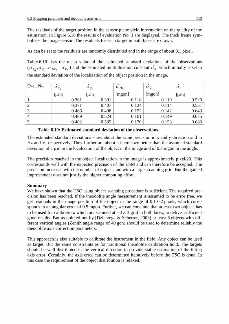
6.3 Mapping parameter and theodolite axis error 113

The residuals of the target position in the sensor plane yield information on the quality of the estimation. In Figure 6.18 the results of evaluation No. 3 are displayed. The thick frame sym-bolizes the image sensor. The residuals for each target in both faces are drawn. As can be seen: the residuals are randomly distributed and in the range of about 0.1 pixel. Table 6.10 lists the mean value of the estimated standard deviations of the observations (

qxσ ,qyσ ,

THzσ , TVσ ) and the estimated multiplication constant 0σ , which initially is set to

the standard deviation of the localization of the object position in the image. Eval. No

qxσ qyσ

THzσ TVσ 0σ

[µm] [µm] [mgon] [mgon] [µm] 1 0.361 0.391 0.118 0.110 0.5292 0.371 0.407 0.124 0.114 0.5513 0.466 0.498 0.152 0.142 0.6434 0.489 0.524 0.161 0.149 0.6755 0.482 0.535 0.170 0.153 0.683

Table 6.10: Estimated standard deviation of the observations. The estimated standard deviations show about the same precision in x and y direction and in Hz and V, respectively. They further are about a factor two better than the assumed standard deviation of 1 µm in the localization of the object in the image and of 0.3 mgon in the angle. The precision reached in the object localization in the image is approximately pixel/20. This corresponds well with the expected precision of the LSM and can therefore be accepted. The precision increases with the number of objects and with a larger scanning grid. But the gained improvement does not justify the higher computing effort. Summary We have shown that the TSC using object-scanning procedure is sufficient. The required pre-cision has been reached. If the theodolite angle measurement is assumed to be error free, we get residuals in the image position of the object in the range of 0.1-0.2 pixels, which corre-sponds to an angular error of 0.5 mgon. Further, we can conclude that at least two objects has to be used for calibration, which are scanned at a 3 × 3 grid in both faces, to deliver sufficient good results. But as pointed out by [Dzierzega & Scherrer, 2003] at least 6 objects with dif-ferent vertical angles (Zenith angle range of 40 gon) should be used to determine reliably the theodolite axis correction parameters. This approach is also suitable to calibrate the instrument in the field. Any object can be used as target. But the same constraints as for traditional theodolite calibration hold. The targets should be well distributed in the vertical direction to provide stable estimation of the tilting axis error. Certainly, the axis error can be determined iteratively before the TSC is done. In this case the requirement of the object distribution is relaxed.

7 Benchmarking To verify the capabilities of the measurement developed and to test the calibration, a bench-mark is defined. This benchmark should point out the potential of an IATS system in terms of accuracy. The limits are evaluated using well-known reference markers of circular shape. Secondly, the capability to measure non-cooperative targets is outlined. A practice related test is done by measuring parts of a historic building in Rheineck/Switzerland, the Löwenhof, and a kinematical test to determine the six degrees of freedom of an object at different positions and from different views.

7.1 Measurement of known circular reference markers To evaluate the limits of the accuracy of an IATS in a natural environment, circular reference markers are measured. Two different test approaches are used to determine the limits. The first approach consists of 19 measurement series on 10 targets spread out over 17 days, while in the second one the targets are measured during several hours. The circular, black target has a small white disc in the center and additionally a symbolized crosshair, which is used for manually aiming to get a reference measurement. The dimensions of the target are defined in Figure 7.1. The diameter of 40 mm of the inner disc assures that the laser spot of the range finder is reflected only from the white part.

150 mm 40 mm

Figure 7.1: Circular reference target.

The base of the target is an achromatically anodized aluminum plate, which is of quadratic shape with a side length of 200 mm. The discs are printed using silk-screening. The targets are mounted on two different buildings at Leica Geosystems (cf. Figure 7.2). Measurements of distances in the range of 50 – 90 m are possible. The angular range is ap-proximately 30 gon horizontally and 10 gon vertically. The aluminum plates are directly screwed on the concrete to guarantee high stability.

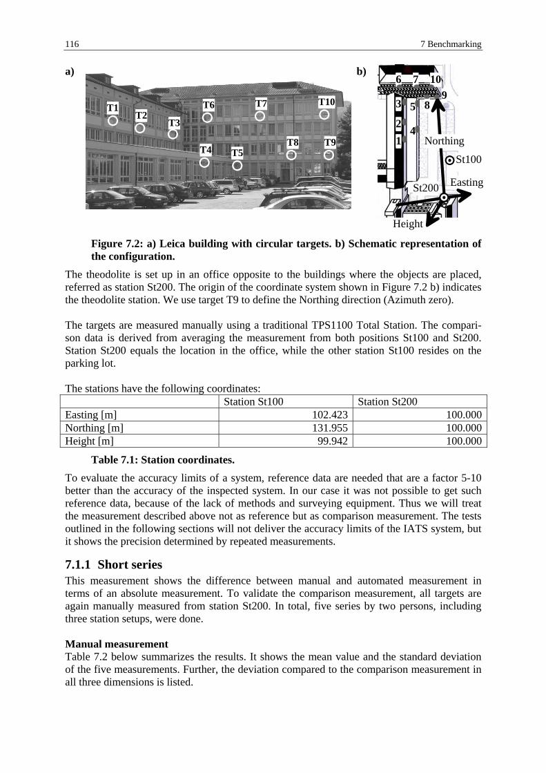
116 7 Benchmarking

a)

T1T2

T3

T6 T7 T10

T4 T5T8 T9

b)

Easting

12

3 5

4

89

10

Northing

Height

6 7

St200

St100

Figure 7.2: a) Leica building with circular targets. b) Schematic representation of the configuration.

The theodolite is set up in an office opposite to the buildings where the objects are placed, referred as station St200. The origin of the coordinate system shown in Figure 7.2 b) indicates the theodolite station. We use target T9 to define the Northing direction (Azimuth zero). The targets are measured manually using a traditional TPS1100 Total Station. The compari-son data is derived from averaging the measurement from both positions St100 and St200. Station St200 equals the location in the office, while the other station St100 resides on the parking lot. The stations have the following coordinates: Station St100 Station St200 Easting [m] 102.423 100.000Northing [m] 131.955 100.000Height [m] 99.942 100.000

Table 7.1: Station coordinates. To evaluate the accuracy limits of a system, reference data are needed that are a factor 5-10 better than the accuracy of the inspected system. In our case it was not possible to get such reference data, because of the lack of methods and surveying equipment. Thus we will treat the measurement described above not as reference but as comparison measurement. The tests outlined in the following sections will not deliver the accuracy limits of the IATS system, but it shows the precision determined by repeated measurements.

7.1.1 Short series This measurement shows the difference between manual and automated measurement in terms of an absolute measurement. To validate the comparison measurement, all targets are again manually measured from station St200. In total, five series by two persons, including three station setups, were done. Manual measurement Table 7.2 below summarizes the results. It shows the mean value and the standard deviation of the five measurements. Further, the deviation compared to the comparison measurement in all three dimensions is listed.

7.1 Measurement of known circular reference markers 117

Mean Value Standard Deviation Difference to compari-son measurement

E [m]

N [m]

H [m]

E [mm]

N [mm]

H [mm]

E [mm]

N [mm]

H [mm]

T1 73.458 156.959 108.132 1.3 0.5 0.9 -0.6 0.9 0.6T2 73.819 165.107 108.099 2.0 0.5 0.7 -1.8 1.1 1.5T3 74.404 178.459 108.213 2.5 1.2 0.9 -1.8 1.0 1.9T4 84.053 161.788 102.973 2.8 1.1 0.4 -2.2 3.9 1.3T5 84.899 181.067 102.959 2.9 0.9 0.8 -1.1 1.6 2.2T6 78.308 186.713 111.812 1.3 0.9 0.8 -4.6 10.6 4.8T7 87.904 186.303 111.814 1.5 1.1 0.8 -0.9 3.9 2.8T8 93.627 186.049 104.785 2.6 0.7 0.7 -0.7 2.5 3.0T9 100.000 185.775 104.789 2.6 1.5 1.1 -0.4 3.6 1.8T10 99.131 185.818 111.822 1.9 2.8 1.0 -0.2 3.2 2.5Avg. − − − 2.1 1.1 0.8 -1.4 3.2 2.2

Table 7.2: Result of the manual measurement on the circular targets from station St200.

The achieved standard deviation in the average is about of 2.5 mm in all three dimensions. The difference compared with the comparison measurement ranges from –5 mm up to 10 mm, while in the average we have a difference of approximately 2−3 mm. Mainly for target T6 a difference of 10 mm in the Northing is noted. The same problem occurs in the comparison measurement on T6. Thus, this effect can be explained by an erroneous distance determina-tion caused by the bad angle of incidence of the laser beam. Automatic measurement The discs are automatically measured using the measurement procedures described in sec-tion 5.3.1. The discs are determined either using disc matching or by matching several edge segments at the disc border (Tangent matching). Table 7.3 presents the summarized results of 19 single measurement series on 10 targets at different positions spread out over 17 days and under different weather conditions. One measurement procedure on a target consists of 5 sin-gle shots without moving the theodolite. The outliers are detected by comparing the results of the single shots with the median. If the deviation is bigger than 10 mm, the measurement is not accepted. The disc matching produced 1 outlier for target T5, while in the tangent match-ing we had 6 outliers for Target T3, 3 outliers for T5 and 13 outliers for T9. Those outliers have to be seen with respect to 950 single measurements (19 series × 10 targets × 5 single shots). The results for the disc matching in Easting and Height are a factor two better than those de-termined with the tangent matching (Table 7.3). Easting and Height are mainly influenced by the angular measurement, this means by image processing, while Northing mainly depends on the distance measurement, because the pointing direction is towards Northing. This explains, why no difference in the Northing coordinate between both measurements can be seen. From this test, we can derive that the disc matching approach leads to more stable results than those of the tangent matching.

118 7 Benchmarking

Standard deviation for the disc match-ing

Standard deviation for the tangent matching

Target E [mm] N [mm] H [mm] E [mm] N [mm] H [mm] T1 0.8 1.0 0.8 0.8 1.0 0.8 T2 1.4 2.4 1.4 1.5 2.4 1.5 T3 0.8 2.6 0.8 5.1 2.6 5.1 T4 1.4 2.6 1.4 1.5 2.6 1.5 T5 1.3 2.9 1.3 3.4 2.9 3.4 T6 0.6 1.0 0.6 0.7 1.0 0.7 T7 1.3 3.3 1.3 1.0 3.3 1.0 T8 1.2 3.0 1.2 1.2 3.0 1.2 T9 1.3 2.6 1.3 8.3 2.7 8.3 T10 1.5 2.6 1.5 1.4 2.6 1.4 Avg. 1.1 2.4 1.1 2.6 2.4 2.6

Table 7.3: Standard deviation of the automated measurements using disc and tan-gent matching.

The results above describe only the repeatability of the measurement. But we are also inter-ested in the deviation to the comparison measurement. Figure 7.3 shows the deviation of the mean value of each of the 19 measurements from the comparison value.

Figure 7.3 Variation of the measurement results, comparing the automated meas-urements with the comparison data.

Again, a higher variation in the Northing direction compared with Easting and Height can be noted. The deviation from the comparison measurement in general is below 10 mm and in the lateral (Easting and Height) below 5 mm. Summarizing the manual and the automated measurement Figure 7.4 summarizes the results and shows the deviation of the manual and the automatic measurement from the comparison measurement for the targets: T1, T4, T7, T8 and T9. On the left the difference is calculated using the raw measurement data and on the right, the measurements are corrected by a systematic error. The systematic error equals the mean de-viation of all measurements from the comparison measurement calculated individually in all three dimensions and can be interpret as a station position error.

7.1 Measurement of known circular reference markers 119

Figure 7.4: Summarized results of the manual and automatic measurement on cir-cular targets compared with the comparison measurement. The circles indicate an error radius of ±5 mm and the thin dashed lines describe the pointing directions of the theodolite.

The numbers in the image identify the corresponding targets; the letter T is omitted in order not to overload the image. The dashed thin black lines towards the objects symbolize the pointing direction in the horizontal plane. The circles indicate a range of ±5 mm. The lower part shows the deviation in the horizontal plane, while the upper part shows the error in the Easting-Height-plane. Most of the measurements are within a range of ±5 mm. But a systematic error in the Nor-thing is apparent, obviously indicated by the error for targets T4 and T8 in the horizontal plane. Correcting the systematic error reduces the error variation. We can conclude that this benchmark yields an accuracy of the IATS below 3 mm on well-known circular targets at an object distance up to 90 m.

7.1.2 Long series In contrary to the short series that are done in a time range of several minutes, the long meas-urement series are carried out during several hours. Further, different evaluation methods are compared, as listed below: • Least squares disc matching, as described in section 5.2.3.3. The blur applied to the tem-

plate is set to a fixed value. • Simultaneously to the discs, the position of a prism is measured with a second total sta-

tion. • Least squares disc matching, where the blur is iteratively determined and corrected. • Disc determination by local tangent matching followed by matching an ellipse.

120 7 Benchmarking

• Least squares disc matching applied to sub-sampled images. This simulates an image sen-sor of coarser resolution.

The start parameters for the LSM are determined by normalized cross-correlation using the generated disc template. The measurement consists of many repetitions measuring consecu-tively the different targets. A series of single determinations of the polar angles and the dis-tance defines a repetition. The measurement process is illustrated in Figure 7.5.

Time

T1

Ti

Tm

Repetition 1

Targ

et N

umbe

r Repetition 1

Repetition 2

Repetition 2

Repetition 3

Figure 7.5: Repeated measurement of different targets.

The measurement of a target in a single repetition corresponds to the following measurement procedure: • Set focus lens based on distance measurement • Determine camera constant by online calibration • Roughly detect target using normalized cross-correlation based on the template later used

for LSM • Measure the target several times (single measurements) without changing the focus and

using the same camera constant. Register the following parameters Theodolite pointing angles Theodolite inclination angles Internal temperature Distance Object position in the image determined by LSM

The object polar angles are determined by back-transformation. Several measurements during a day are made. Here we will present a series, where 80 repeti-tions with 5 single measurements each on targets T1, T5, T9 and T10 are done. The meas-urement started at 9 a.m. and lasted 8 hours until 5 p.m.. In the figures the deviation of the measurement value relative to the first measurement will be shown. The x-axis indicates measurement time. The displayed value is calculated as the aver-age of one repetition of the current object, after elimination of all outliers. Different types of outliers can occur. The LSM does not converge to a correct result or the number of optimiza-tion steps exceeds a certain limit. Further it is possible that the camera constant could not be found correctly by the online camera constant calibration. Finally, all measurements in a repe-tition where the deviation from the median exceeds a certain limit (for the angle measure-ments this is 2 mgon) are eliminated. The remaining values of that repetition are averaged to get the final measurement value. If the standard deviation of the remaining values exceeds a limit (for the angle measurements 1 mgon), the measurement value is not used. In the tables below, for example Table 7.4, the number of outliers are listed for each series. Further, the

7.1 Measurement of known circular reference markers 121

standard deviation of the measurements of each target is given. Additionally, the standard deviation is calculated using a moving window of size 10 samples. That means, the standard deviation is calculated for 10 consecutive values, yielding N-9 local standard deviations, cf. Figure 7.6, where N is the number of measurement samples. The average of all those local standard deviations is listed in the tables, e.g. last two columns in Table 7.4 labeled “Std Hz, Mov. window” and “Std V, Mov. window”.

Index

MeasurementValue

Standard deviation iscalculated for a subsetof the data

1 N

Moving Window Moving Window

Figure 7.6: Definition of a moving window. The window is shifted over the meas-urement samples and at each position the standard deviation of the dataset within the window is calculated.

7.1.2.1 Standard evaluation: LSM disc matching Disc matching determines the center and the diameter of the target. The radiometric parame-ters are iteratively estimated and the template is blurred using a Gaussian with σ = 2 pixel. The start parameters are calculated using normalized cross-correlation. The results of the measurements are displayed in Figure 7.7. The variation of the horizontal angle is higher than the variation in the vertical angle. This can be explained by the different pixel size. Because the pixels in vertical direction are 1.5 times smaller than in horizontal direction, the vertical object position in the image can be deter-mined more precise. The factor 1.5 is also identified if the standard deviations in Hz and V are compared, cf. Table 7.4. Target Std Hz Std V # Outliers Std Hz

Mov. window Std V Mov. window

T1 0.22 mgon 0.14 mgon 0 0.16 mgon 0.14 mgonT5 0.35 mgon 0.12 mgon 0 0.23 mgon 0.10 mgonT9 0.25 mgon 0.13 mgon 1 0.15 mgon 0.11 mgonT10 0.26 mgon 0.12 mgon 0 0.19 mgon 0.10 mgon

Table 7.4: Standard deviation and number of outliers for the disc matching. The outlier for target T9 is caused by an erroneous online camera constant calibration. No other outliers were detected. The standard deviation of the angle measurement is below the specified angle accuracy for TPS1100 Series Instruments.

122 7 Benchmarking

Figure 7.7: Measurement results for disc matching.

7.1.2.2 Simultaneously measuring with a second total station using the ATR In the previous evaluation a variation of the inclination in the range of 2 mgon can be seen. This leads to the conclusion that the buildings where the total station is set up and where the targets are mounted are not stationary. Therefore, a second theodolite (TPS1100) is placed 3 m beside the Image Assisted Total Station and 2 prisms are mounted below the targets T5 and T9. With the second total station, the prisms are measured simultaneously to the meas-urement of the IATS on the corresponding discs. The prisms are automatically measured us-ing the automatic target recognition (ATR) function.

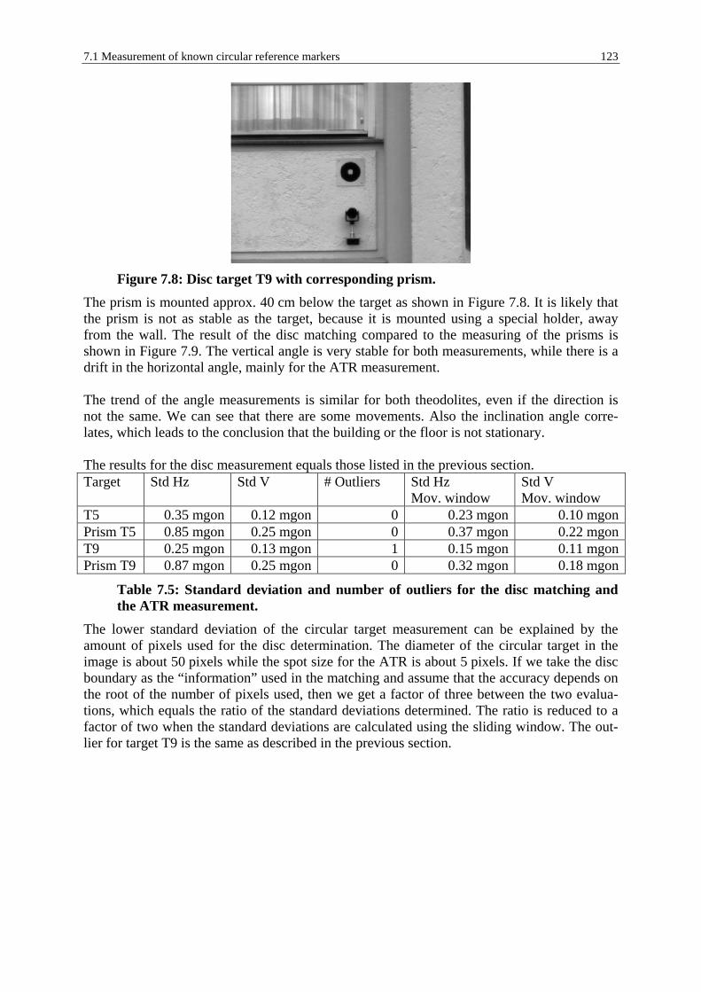
7.1 Measurement of known circular reference markers 123

Figure 7.8: Disc target T9 with corresponding prism.

The prism is mounted approx. 40 cm below the target as shown in Figure 7.8. It is likely that the prism is not as stable as the target, because it is mounted using a special holder, away from the wall. The result of the disc matching compared to the measuring of the prisms is shown in Figure 7.9. The vertical angle is very stable for both measurements, while there is a drift in the horizontal angle, mainly for the ATR measurement. The trend of the angle measurements is similar for both theodolites, even if the direction is not the same. We can see that there are some movements. Also the inclination angle corre-lates, which leads to the conclusion that the building or the floor is not stationary. The results for the disc measurement equals those listed in the previous section. Target Std Hz Std V # Outliers Std Hz

Mov. window Std V Mov. window

T5 0.35 mgon 0.12 mgon 0 0.23 mgon 0.10 mgonPrism T5 0.85 mgon 0.25 mgon 0 0.37 mgon 0.22 mgonT9 0.25 mgon 0.13 mgon 1 0.15 mgon 0.11 mgonPrism T9 0.87 mgon 0.25 mgon 0 0.32 mgon 0.18 mgon

Table 7.5: Standard deviation and number of outliers for the disc matching and the ATR measurement.

The lower standard deviation of the circular target measurement can be explained by the amount of pixels used for the disc determination. The diameter of the circular target in the image is about 50 pixels while the spot size for the ATR is about 5 pixels. If we take the disc boundary as the “information” used in the matching and assume that the accuracy depends on the root of the number of pixels used, then we get a factor of three between the two evalua-tions, which equals the ratio of the standard deviations determined. The ratio is reduced to a factor of two when the standard deviations are calculated using the sliding window. The out-lier for target T9 is the same as described in the previous section.

124 7 Benchmarking

Figure 7.9: Comparing the results of the disc matching with those of the ATR measurements.

From this experiment we can derive that movements of the floor and the buildings can explain some drifts of the measured object angle.

7.1.2.3 Disc LSM with additionally estimating the blur In the standard measurement a constant blur is applied generating the template used for LSM. Now, we want to inspect the influence, if the blur is iteratively estimated during the LSM process, cf. section 5.2.3.5.

7.1 Measurement of known circular reference markers 125

The same images and measurements as for the standard evaluation are used. The only differ-ence is that a modified LSM algorithm determines the object position, where the blur is itera-tively estimated. Again, we will compare the results of the standard evaluation, referred to as ‘T_ ref’, with the results of additionally estimating the blur, referred to as ‘T_ blur’. Figure 7.10 below shows the results for the targets T5 and T9, the same as used in the previous section.

Figure 7.10: Comparing the results of the standard disc matching with those of the disc matching extended by estimating the blur.

It is hardly possible to distinguish between the two evaluations. Both lead to the same results. If we look closer at the standard deviation, only a slight difference in the horizontal angle is noted. But we can conclude that both evaluations yield the same precision. Target Std Hz Std V # Outliers Std Hz

Mov. window Std V Mov. window

T5 ref 0.35 mgon 0.12 mgon 0 0.23 mgon 0.10 mgonT5 blur 0.40 mgon 0.14 mgon 0 0.26 mgon 0.11 mgonT9 ref 0.25 mgon 0.13 mgon 1 0.15 mgon 0.11 mgonT9 blur 0.25 mgon 0.14 mgon 1 0.15 mgon 0.11 mgon

Table 7.6: Standard deviation and number of outliers for the disc matching and the disc matching extended by estimating the blur.

For target T9 we have again the outlier caused by the erroneous camera constant determina-tion. Because both results are equal and the LSM with blur estimation increases the amount of computation, it is not recommended to iteratively estimate the blur.

7.1.2.4 Disc determination by local tangent matching followed by ellipse fitting Another method to determine the center of the disc is to match several tangents, short step edge segments, at the disc border followed by matching an ellipse into those tangent points. The results are referred to as ‘T_ edge’. In this experiment 8 matching positions, equally dis-tributed around the disc, are used. The benefit of such an approach is that the templates for the step edge have 30 times less pixel than that for the disc, which will decrease the computing time. But the occurrence of mismatches will increase, which requires robust outlier detection. For the same targets as above the results of the standard disc-matching algorithm are com-pared with the tangent matching-algorithm.

126 7 Benchmarking

Figure 7.11: Comparing the results of the standard disc matching with those of the tangent matching.

The precision of both approaches are comparable and in the same range. But according to Table 7.7 there are significantly more outliers for the tangent matching. Target Std Hz Std V # Outliers Std Hz

Mov. window Std V Mov. window

T5 ref 0.35 mgon 0.12 mgon 0 0.23 mgon 0.10 mgonT5 edge 0.47 mgon 0.13 mgon 9 0.42 mgon 0.11 mgonT9 ref 0.25 mgon 0.13 mgon 1 0.15 mgon 0.11 mgonT9 edge 0.32 mgon 0.13 mgon 9 0.21 mgon 0.11 mgon

Table 7.7: Standard deviation and number of outliers for the disc matching and the tangent matching.

The outliers are caused by a too high standard deviation between the five single measure-ments in a single repetition. We can conclude that this matching method is not to be used without developing more reliable outlier detection or by matching more local tangents. But this would increase the computing power and the benefit of smaller templates is lost.

7.1.2.5 Checking the influence of sub-sampling This experiment examines the influence of using fewer pixels on the precision. The original image is sub-sampled, meaning that n×n pixels are averaged to one new pixel. The results are calculated using the images and measurements on target T5. The object position is determined with the standard evaluation using disc matching. We will apply sub-sampling factor 1, which equals the standard measurement, and further the factors 2, 4 and 6. The maximal factor 6 corresponds to a pixel size of 59×38 µm. Using the same image sensor but widening up the field of view of the optics could cause a similar effect. Thus this experiment gives information about the precision to expect with a wider field of view.

7.1 Measurement of known circular reference markers 127

Figure 7.12: Comparing the results for different sub-sampling factors using tar-get T5.

Target Sub-samp.

Factor Std Hz Std V # Outliers Std Hz

Mov. window Std V Mov. window

T5 1 0.35 mgon 0.12 mgon 0 0.23 mgon 0.10 mgon 2 0.44 mgon 0.15 mgon 0 0.29 mgon 0.11 mgon 4 0.66 mgon 0.20 mgon 0 0.45 mgon 0.16 mgon 6 1.09 mgon 0.29 mgon 0 0.77 mgon 0.21 mgon

Table 7.8: Standard deviation and number of outliers for different sub-sampling factors using target T5.

The standard deviation increases by a factor of 2 to 3 where the number of pixels is reduced by factor 36 for sub-sampling factor 6. But we have to be careful that this can only be done if the target is of sufficient size. In case of no sub-sampling, the disc diameter is 50 pixels. For sub-sampling factor 6 the diameter is still approx. 8 pixels, which is sufficient to apply LSM. According to the results, the field of view could be extended by a factor of 2 without loosing too much precision and still fulfilling the specification of a TPS1100 Series Instrument.

7.1.3 Conclusions of the section 7.1 We compared the absolute measurements of circular targets employed with the IATS with manual measurements using a total station from the same series as the IATS prototype. The comparison of both measurements leads to a conformity of 3-5 mm, where the difference is mainly caused by the distance measurement. Further the precision of the measurement during a period of several hours satisfies the requirement of a standard deviation of the angular measurement of 0.5 mgon equal to that of a TPS1100 instrument. The disc matching approach applying a fixed blur to the template provides the best results. In this benchmark the average of five single shots is used as the final measurement value. That means, the distance measuring and the matching is performed 5 times. Even that those repeti-tions can be calculated efficiently, the distance is known from the first measurement and thus no adjustments are needed and for the matching the same start points and parameters can be used as in the previous calculation, it needs more time than a single shot. To increase the pre-cision and to detect outliers three single shots should be employed. But because no outliers due to measurement inconsistency are detected in the circle matching, measurements with only one single shot are best practice in standard applications.

128 7 Benchmarking

7.2 Measurement of non-cooperative, structured targets The measurement of non-cooperative, structured targets is the purpose of an IATS. Thus, the benchmarking is extended to non-signalized targets. We will present two different measure-ment setups. One uses the same scene outdoors as used for the disc measurement. There, points defined by two intersecting lines are evaluated and compared with a comparison meas-urement. A second benchmarking is done inside, where objects of different shape, such as corner, cylinder, bar and disc are used. For those targets the repeatability of the measurement is evaluated.

7.2.1 Point measurement results outdoors In Figure 7.13 the scene used is shown together with the four objects to be measured. All four objects are corners of windows. The station setup and comparison measurement is exactly the same as for the disc benchmark. a)

N11

N16

N9

N1

b)

Easting

N1

N9

Northing

Height

N11 N16

St200

St100

Figure 7.13: a) Leica building with natural targets specified. b) Schematic of the setup configuration with the two station positions St100 and St200 and the object labeling.

Figure 7.14 shows a detailed view of the targets. The angle of incidence of the laser beam on the targets N1 and N9 is in the range of 15−25 gon and for the targets N11 and N16 almost perpendicular in a range of 85−95 gon. The corner-like lines indicate the lines approximating the objects, while the crosses define the positions where to measure the distances.

N1 N9 N11 N16

Figure 7.14: Detailed view of all four targets with lines approximating the object to be measured and a cross indicating where to measure the distance.

The same procedure as for the long series used in the disc measurement is applied here. To-tally 42 repetitions were done and each repetition consists of five single measurements. The series lasts from 10 a.m. until 4 p.m. The horizontal and vertical angles are determined using

7.2 Measurement of non-cooperative, structured targets 129

the back-transformation algorithm. The distance is only measured at one specified point that is manually defined. The object position in the image is calculated using the measurement procedure for objects defined by the intersection of two lines explained in section 5.3. The results relative to the first measurement are shown below.

Figure 7.15: Results for all targets. There are drifts for the polar angles, but they are small and they correlate with the tempera-ture. Thus, a movement of the object could cause this, as we have seen in the evaluation of the disc targets in conjunction with the ATR measurement. The variation of the distance of the targets N1 and N9 is significantly higher than those of the other two targets. The reason for this could be the bad angle of incidence of the laser beam on these targets.

130 7 Benchmarking

Target Std Hz Std V # Outliers Std Hz Mov. window

Std V Mov. window

N1 0.24 mgon 0.17 mgon 0 0.17 mgon 0.12 mgonN9 0.27 mgon 0.18 mgon 0 0.18 mgon 0.14 mgonN11 0.39 mgon 0.18 mgon 0 0.32 mgon 0.12 mgonN16 0.34 mgon 0.17 mgon 0 0.25 mgon 0.13 mgon

Table 7.9: Standard deviation and number of outliers for natural targets. The standard deviation for horizontal and vertical angles is in the same range as evaluated in the disc benchmark. No outliers were detected. But this gives no information on the 3D coor-dinates measured. Thus, in the following we will compare with the comparison coordinates listed below.

3D Coordinates Difference between station St100 and St200 measurement

Easting [m]

Northing [m]

Height [m]

Easting [mm]

Northing [mm]

Height [mm]

N1 73.869 165.536 110.822 5 -31 -5N9 84.241 164.745 103.251 9 -26 2N11 78.030 186.513 110.706 8 -1 1N16 92.271 185.899 114.240 -4 3 1

Table 7.10: 3D coordinates of the natural targets determined by a comparison measurement.

Additionally to the 3D coordinates the difference between the manual measurement from the two stations, St100 and St200, are listed. The difference has two significant outliers for the Northing direction for the targets N1 and N9. This comes from the same effect as described above caused by the distance measurement. In Figure 7.16 the differences between manual and comparison measurements are shown. This figure has similar outline as Figure 7.4, where the dashed thin black line towards the objects symbolize the pointing direction in the horizontal plane and the circles show an error range of ±5 mm. The two targets aimed at more or less orthogonal (N11 and N16) show high accuracy, while the other two (N1 and N9) have a deviation from the comparison up to 40 mm in pointing direction. We can conclude that it is extraordinary important to measure the distance at the correct posi-tion. The angle of incidence of the EDM beam is mainly responsible for an erroneous distance measurement. Thus, the objects to be measured should be aimed at incidence angles near 90°. Otherwise, we can produce an error in pointing direction that leads to erroneous 3D coordi-nates. An approach against this effect is to measure the plane wherein the object lies and in-tersect this plane with the pointing direction. In the next section we shall evaluate this ap-proach.

7.2 Measurement of non-cooperative, structured targets 131

Figure 7.16: Difference between the manual and the comparison measurement. The circles indicate an error range of ±5 mm and the thin dashed line describes the pointing direction of the theodolite.

7.2.2 Object measurement results indoors The benchmarking done indoor focuses on the measurement of targets of different shapes. We will measure the precision in a repeated measurement on the same target during several hours. The measurement algorithms developed in section 5.3 are tested using a corner-like object and a wooden bar on a stucco wall, a heating pipe and a circular target, namely a power socket. Further, the influence of the distance measurement approach, either using only one shot at a distinct position or to measure a plane by three points and intersect it with the point-ing direction, is inspected. The numbering of the measurement is chronological and does not match the sequencing in the following sections.

7.2.2.1 Corner measurement We will point out the difference between measuring an object either using line intersection in conjunction with multiple, local edge matching or using a corner template and only matching once. For corner matching only the border part of the corner template is used. Further the in-fluence of the distance measurement is investigated. There are two possibilities to determine the object distance. One is measuring the distance by a single shot and the other is to measure three points in 3D and determine the plane wherein the object lies. Then the pointing direction is intersected with this plane yielding the distance. The four possibilities investigated of measuring the same object are illustrated in Figure 7.17. We will use an identification number of each measurement even if it is the same object. Addi-

132 7 Benchmarking

tionally to the approximation lines and the position where to measure the distance (cross) the length of the lines is given. This defines the size for the corner template and gives a relation to the number of pixels used in the match0ing. The distance to the object is 11.6 m. Line Matching and Intersecting Corner Matching Single distance measure-ment

I4

I6

Line length 174 and 122 pixels 44 and 28 pixels Plane measurement I5

I7

Line length 167 and 181 pixels 24 and 41 pixels

Figure 7.17: Definition of the four different approaches to measure a corner like object.

The results of 17 repetitions with 5 single measurements during 8 hours are listed below. We will treat the average of the 5 single measurements as the measurement result. There is a sys-tematic difference between the two-line-intersection and the corner-matching measurement for the horizontal angle, cf. Figure 7.18. The difference of 3 mgon at 11.6 m corresponds to a shift of only 0.5 mm, which thus can be caused by the different fitting procedure of the tem-plates. Further, there is a constant difference between the distance determined by a single shot (I4 and I6) and by the intersection of the pointing direction with a plane (I5 and I7). The dif-ference is in the order of 6 to 8 mm, which again points out the importance of a correct dis-tance measurement. Target Std Hz Std V # Outliers Std Hz

Mov. window Std V Mov. window

I4 0.46 mgon 0.39 mgon 0 0.36 mgon 0.27 mgonI5 0.45 mgon 0.34 mgon 0 0.36 mgon 0.22 mgonI6 0.54 mgon 0.65 mgon 0 0.37 mgon 0.40 mgonI7 0.48 mgon 0.55 mgon 0 0.35 mgon 0.40 mgon

Table 7.11: Standard deviation and number of outliers for the corner target. The standard deviation of the two-line-intersection is up to a factor 2 better than the results of the corner matching. This is explainable by the number of pixels used for the matching, which is significantly higher for the two-line-intersection.

7.2 Measurement of non-cooperative, structured targets 133

Figure 7.18: Results of the corner measurement, relative to the first measurement of repetition I4.

Talking about robustness, we can mention one important effect to consider. When measuring another object than described above, where the illumination is not this homogeneous, some outliers occur. Because of illumination effects, there were some bright spots nearby the edge. Those spots shifted the edge to the right, Figure 7.19. Line 2 is taken instead of the line 1, because it better fits the manually placed lines in terms of distance and angle between the lines.

Line 1 Line 2

Figure 7.19: Shift of an edge due to illumination effects.

This problem can be overcome by user interaction. If there are ambiguities, the user must de-cide, which line to be used for further computation. Another approach to solve the ambiguities

134 7 Benchmarking

is to use the fact that the object to be measured is a corner and thus use the properties of a line and a corner.

7.2.2.2 Space vector Not always a single point is of interest, but the orientation vector of an object. Therefore, we will measure the central line of a wooden bar, which is defined as the middle line of the two borderlines, Figure 7.20. It is about the same object as for the corner measurement discussed in the previous section.

Figure 7.20: Wooden bar on a stucco wall.

The purpose of this measurement is to determine the boundary lines of the bar in the image and thereof derive the central line. Then, five pointing directions corresponding to points on the central line are calculated and thereon the distance is measured. Finally a 3D line is fitted into the resulting five points yielding the direction vector of the central line. The results are displayed relative to the average pointing vector b0. Two different parameters are evaluated. The angle variation, meaning the angular deviation of any measurement compared with the average pointing direction, Figure 7.21 a). The difference is calculated using the dot product. Secondly the orthogonal distance s between any line and the average line as shown in Figure 7.21 b) is computed. The length of the central lines is approximately 200 mm, which equals the size of the field of view for an object distance of 11 m. a)

b0

bi

ϕ

b)

s

b0

bi

Figure 7.21: a) Definition of the variation of the pointing vector. b) Distance be-tween arbitrary pointing directions relative to the average pointing direction.

The measurement lasts 8 hours and 17 repetitions were measured. The results in Figure 7.22 show a precise repeatability of the pointing vector, as well as for the angular variation and for the distance between the pointing vectors

7.2 Measurement of non-cooperative, structured targets 135

Figure 7.22: Results of measuring the wooden bar.

The standard deviations indicate a high precision and no outliers were detected. The high pre-cision could be explained both by the small range taken into consideration and the good re-flectance of the object provide stable distance measurement. Note that the unit of the variation of the pointing direction is given in gon. Value Std Std

Mov. window #Outliers

Pointing direction 0.016 gon 0.017 gon 0Vector distance 0.024 mm 0.019 mm 0

Table 7.12: Standard deviations of the pointing direction. The result of the measurement can be compared with the one measuring corners. Figure 7.23 illustrates, how the pointing direction of the central line is determined using two separate cor-ner measurements. The left and the right corner are measured and the pointing direction is computed by the vector difference of both corners in 3D. This pointing difference is com-pared to the one obtained by measuring the central line of the bar. The vector based on the corner measurement equals the average of multiple measurements and is taken as reference.

Figure 7.23: Measuring the direction of the wooden bar by determining the center line or by measuring two corners and calculating the difference vector.

Because the distance is not measured on the same line for both measurements, we will only compare the direction vector of the measurement and not the absolute position.

136 7 Benchmarking

Figure 7.24: Pointing difference between central line and corner measurement.

From the figure above we see, that the mean difference is in the range of 0.45 gon. This equals a shift of 7 mm for a vector length of 1 m. This systematic offset between both vectors could be caused by the fact that the boundary lines of the wooden bar are not exactly parallel.

7.2.2.3 Pole measurement A heating pipe is measured similarly to the wooden bar. It is not an easy task to measure cy-lindrical objects using total stations, because first the boundary is determined by manually measuring the pointing angles and there from the middle of the cylinder is aimed to measure the distance. A second way is to continuously measure the distance and stop measuring when the nearest distance is found. This position corresponds to a point on the central line of the cylinder .The IATS simplifies this procedure. The central line of the pipe is determined by image processing and the distance is then measured at several positions on this central line (cf. Figure 7.25).

Centralline

Positionsto measurethe distance

Boundarylines

Figure 7.25: Heating pipe approximated by two lines, derived central line and posi-tions where to measure the distance.

The results are organized as those of the wooden bar. The variation of the pointing vector and the distance between the vectors is calculated and illustrated in Figure 7.26, while the stan-dard deviations are listed in Table 7.13.

7.2 Measurement of non-cooperative, structured targets 137

Figure 7.26: Results of measuring the heating pipe.

Value Std Std Mov. window

#Outliers

Coaxial pointing direction 0.042 gon 0.037 gon 0Vector distance 0.027 mm 0.022 mm 0

Table 7.13: Standard deviations of the pointing direction. The precision reached is about a factor two worse than the results of the wooden bar. The maximal error of 0.15 gon equals a shift of 2.3 mm for a pole length of 1 m. The pole measurement can be used in hidden point applications, where the direction of a pole of known length and diameter is determined to measure a ground point not in the field of view.

7.2.2.4 Circular target measurement (Socket) It is not possible to approximate all objects with linear boundaries. Thus, tangents are used to locally determine boundary points. Using those points and a geometrical model of the object, a description in 3D can be derived. The object used in this experiment is a power socket. To-tally 31 repetitions with 5 single shots each are measured. The measurement lasts 3 hours. a) I2

b) I3

Figure 7.27: Determine a disc by measuring five tangential points on the disc boundary. a) Pointing direction is intersected with a plane defined by 3 points. b) For each tangent the distance is separately measured.

Proceeding two different measurements, where once the pointing directions are intersected with a plane, I2, and secondly for each tangent the distance is measured separately, I3 (cf. Figure 7.27). The plane intersection approach will reduce measurement time because only three points have to be measured compared with multiple distance measurement for each tan-gent. Because of the object shape it is not possible to measure the distance at the front surface

138 7 Benchmarking

of the socket. Thus, the distance is measured to the wall behind the socket. This offset does not corrupt the measurement results, because it can be seen as constant for all positions.

Figure 7.28: Position of the disc center relative to the first measurement of I2 and the disc radius.

The measurement results are displayed relative to the first measurement of I2 (cf. Figure 7.28). The variation of the disc center in 3D and the radius are printed. There is a sys-tematic offset between the two series for the disc center and likewise for the disc radius. The reason for this could be that the socket sticks out the wall, which result in an offset. Disc center Std Std

Mov. window #Outliers

I2 0.07 mm 0.05 mm 0I3 0.06 mm 0.04 mm 0

Table 7.14 Standard deviation of the disc center position. Radius Std Std

Mov. window #Outliers

I2 0.02 mm 0.01 mm 0I3 0.03 mm 0.01 mm 0

Table 7.15: Standard deviation of the radius. The standard deviation of the center and the radius (Table 7.14 and Table 7.15) indicate a high repeatability, but we have to consider that a shift of 0.05 mm at an object distance of 11 m results in an angular shift of 0.3 mgon, which is the expected precision. A possible error source in object boundary detection is illustrated in Figure 7.29. If the illu-mination is not ideal, it is likely that not the correct edge is used for tangential matching. In the left image, the wrong edge where the socket is mounted on the wall is chosen, while in the right image the correct one is taken.

7.3 Application examples 139

Figure 7.29: Ambiguity and illumination problem.

To solve ambiguities user interaction is used as already mentioned in section 7.2.2.1.

7.3 Application examples The results of the above benchmarking are now verified in a practice test to outline the current limits of an IATS. Surveying of architectural parts of the Löwenhof in Rheineck (Switzer-land) defines a first test. A second one is a kinematics test, where a robot station moves around a solid test body. The total station has to determine the actual six degrees of freedom of the test body.

7.3.1 Löwenhof in Rheineck Measuring different objects on the facade of the Löwenhof should give an impression of the capabilities and limitations of the IATS in practice. Figure 7.30 a) shows an image of the front facade of the Löwenhof, while in b) the situation and the definition of the local coordinate system is given. The total station is set up on three different stations (100, 101 and 102) to provide different views of the objects. a)

b)

100

101

102

Löwenhof

N

E

Figure 7.30: a) Image of the front and parts of the east (in the local coordinate sys-tem) facade of the Löwenhof. In front the tripod is setup over station 100. b) Re-cording configuration, three stations (100, 101 and 102) and definition of the local coordinate system.

Table 7.16 lists the station coordinates and the actual height of the instrument. Station Easting [m] Northing [m] Height [m] Instrument height [m] 100 100.000 100.000 400.000 1.687101 88.496 114.829 399.695 1.616102 69.898 121.174 399.815 1.607

Table 7.16: Station coordinates.

140 7 Benchmarking

We had beautiful and warm weather during the measurement campaign. Thus, heating up ef-fects caused by the sun are likely.

50 51

60-69

20

21

22 25 27

26

2423

200 201

202203

205

206 207

204

300

- 322

400

- 422

Figure 7.31: Definition of the five objects measured in the benchmarking: Window head (200 − 207), capital (50, 51), volute (60 − 69), window frieze (20 − 26) and pil-lar (300 − 322 and 400 − 422).

In Figure 7.31 the five objects measured are defined and the distinct object points are num-bered. In the Table 7.17, the objects and the goal of the measurement is clarified. Object Point Numbers Measurement goal Capital 50 and 51 Both points are measured from all three stations Window frieze 20 − 27 All points are measured from stations 101 and 102 Window head 200 − 207 All points are measured from all three stations. The

points 202 - 205 are not geometrically defined. There-fore, different points from all three stations are meas-ured. Those points are used to define the arc.

Volute 60 − 69 The volute is measured from all three stations. The single points are chosen as tangent points on the vo-lute. They do not correspond to each other from the different stations. The goal is to get 3D points of the volute from each station to fit a curve describing the object.

Pillar 300 − 322 and 400 − 422

The pillar is only measured from station 102.

Table 7.17: Detailed description of the measured objects. In the following sections, the results of the measurements are described.

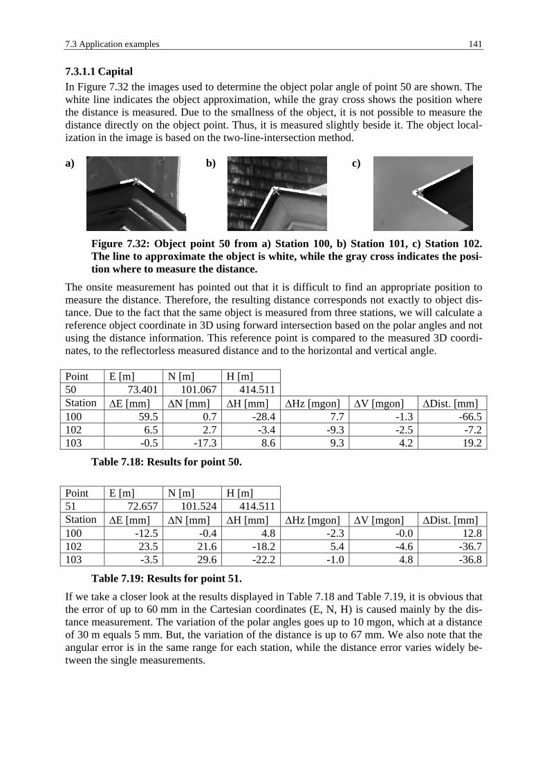
7.3 Application examples 141

7.3.1.1 Capital In Figure 7.32 the images used to determine the object polar angle of point 50 are shown. The white line indicates the object approximation, while the gray cross shows the position where the distance is measured. Due to the smallness of the object, it is not possible to measure the distance directly on the object point. Thus, it is measured slightly beside it. The object local-ization in the image is based on the two-line-intersection method. a)

b)

c)

Figure 7.32: Object point 50 from a) Station 100, b) Station 101, c) Station 102. The line to approximate the object is white, while the gray cross indicates the posi-tion where to measure the distance.

The onsite measurement has pointed out that it is difficult to find an appropriate position to measure the distance. Therefore, the resulting distance corresponds not exactly to object dis-tance. Due to the fact that the same object is measured from three stations, we will calculate a reference object coordinate in 3D using forward intersection based on the polar angles and not using the distance information. This reference point is compared to the measured 3D coordi-nates, to the reflectorless measured distance and to the horizontal and vertical angle. Point E [m] N [m] H [m] 50 73.401 101.067 414.511 Station ∆E [mm] ∆N [mm] ∆H [mm] ∆Hz [mgon] ∆V [mgon] ∆Dist. [mm] 100 59.5 0.7 -28.4 7.7 -1.3 -66.5102 6.5 2.7 -3.4 -9.3 -2.5 -7.2103 -0.5 -17.3 8.6 9.3 4.2 19.2

Table 7.18: Results for point 50. Point E [m] N [m] H [m] 51 72.657 101.524 414.511 Station ∆E [mm] ∆N [mm] ∆H [mm] ∆Hz [mgon] ∆V [mgon] ∆Dist. [mm] 100 -12.5 -0.4 4.8 -2.3 -0.0 12.8102 23.5 21.6 -18.2 5.4 -4.6 -36.7103 -3.5 29.6 -22.2 -1.0 4.8 -36.8

Table 7.19: Results for point 51. If we take a closer look at the results displayed in Table 7.18 and Table 7.19, it is obvious that the error of up to 60 mm in the Cartesian coordinates (E, N, H) is caused mainly by the dis-tance measurement. The variation of the polar angles goes up to 10 mgon, which at a distance of 30 m equals 5 mm. But, the variation of the distance is up to 67 mm. We also note that the angular error is in the same range for each station, while the distance error varies widely be-tween the single measurements.

142 7 Benchmarking

7.3.1.2 Window frieze The measurement of the window frieze is rather similar to the capital measurement, but the possibility to measure the distance is much better, because the laser beam of the range finder can be placed near the object. Two views for the object point 22 from station 101 and 102 are shown in Figure 7.33. a)

b)

Figure 7.33: Object point 22 from a) Station 101, b) Station 102.

We will use the same evaluation as above and calculate the reference point using forward in-tersection using the horizontal and vertical angle. The object point in the image is determined using the two-line-intersection method. Due to the better distance measurement possibility provided by the shape of the object, we expect a higher accuracy for the Cartesian coordi-nates. Pnt. No. Station ∆E

[mm] ∆N [mm]

∆H [mm]

∆Hz [mgon]

∆V [mgon]

∆Dist. [mm]

20 101 -2.9 -7.0 4.5 0.1 -6.5 9.2 102 9.1 -22.0 2.5 1.0 4.8 23.621 101 1.2 3.7 1.0 0.1 -5.2 -3.3 102 -3.8 8.7 -4.0 0.8 3.8 -10.022 101 0.8 1.4 1.8 0.1 -5.7 -1.4 102 2.8 -6.6 -0.2 0.8 4.2 7.023 101 2.0 5.0 0.2 0.1 -5.1 -5.3 102 2.0 -5.0 -0.8 0.7 3.8 5.124 101 4.1 8.2 -1.0 0.1 -4.6 -8.2 102 -12.9 29.2 -8.0 0.7 3.4 -32.525 101 1.4 2.8 0.3 0.1 -4.9 -2.7 102 -8.6 19.8 -6.7 0.7 3.7 -22.526 101 -0.8 -1.0 1.0 0.2 -4.1 1.0 102 1.2 -4.0 0.0 0.6 3.1 4.527 101 -2.0 -3.5 2.4 0.2 -5.0 4.3 102 -5.0 12.5 -4.6 0.8 3.9 -13.6

Table 7.20: Results for the window frieze, points 20 − 27, measured from stations 101 and 102.

The results in Table 7.20 show significantly better results than for the capital. The measure-ments with an error higher than 15 mm are marked in light gray. Again the same effect caused by the distance measurement can be noted. The horizontal location is reasonably precise, while the vertical precision of maximal 6.5 mgon equals a displacement of about 3 mm, which is still within the expected limits. The variation of the distance measurement can also be explained by the bad angle of incidence of the laser beam for station 102. In connection with the laser placement besides the object, this can lead to an erroneous object distance. The fact that higher errors only occur for measurements from station 102 emphasizes this.

7.3 Application examples 143

Due to bad illumination and the gray color of the object, it can happen that an edge cannot be identified in the image.

7.3.1.3 Window head The window head consists of two parts, the four points 200, 201, 206 and 207, which we as-sume to be on a straight line and the points 201−206 defining the arc. The image of object point 206 from the three stations is shown in Figure 7.34. a)

b)

c)

Figure 7.34: Object point 206 from a) Station 100, b) Station 101, c) Station 102

We will distinguish two different evaluations. First the points defining the straight line are compared with a reference point calculated again by forward intersection. Second a disc is fitted into the points defining the arc. The deviation of the measured points from the arc and the variation of the radius between the different measurements are compared. The results for the points on the straight line are listed in Table 7.21. The point 200 could not be measured form station 102, because no distance information is available. Pnt. No. Station ∆E

[mm] ∆N [mm]

∆H [mm]

∆Hz [mgon]

∆V [mgon]

∆Dist. [mm]

200 100 3.9 3.9 -1.6 10.8 -0.6 -3.5 101 11.9 5.9 -9.6 -15.7 3.2 -15.2 102 ---- ---- ---- ---- ---- ----201 100 -15.5 0.5 7.3 1.9 0.1 16.4 101 1.5 0.5 0.3 -2.1 -3.4 -0.2 102 2.5 -12.5 6.3 3.1 3.0 14.3206 100 16.5 3.8 -13.9 8.6 11.9 -20.5 101 6.5 -7.2 -6.9 -30.0 17.1 -3.2 102 -1.5 0.8 13.1 3.0 -30.0 6.3207 100 -2.7 2.1 3.3 5.2 -3.2 3.8 101 7.3 6.1 -4.7 -3.5 -2.4 -10.9

Table 7.21: Results for the points 200, 201, 206 and 207. Besides the point 206, the results are within the same accuracy as the previous evaluations. Measuring the false object edge for point 206 from station 101 causes a difference of 30 mgon in Hz and V, cf. Figure 7.34. The main problem in measuring the window head is that the object border is round. Thus, there is no distinct edge that defines the object. The object bor-der changes for different viewing angles. To evaluate the measurement of the arc, we project the measured points on a plane fitted into the measured 3D points. This assumes that the front of the window head lies in a plane. The orthogonal distances of the object points from the fitted plane are in the range of ±12 mm (Figure 7.35) and this confirms the assumption. The standard deviation of the orthogonal dis-tances for the measurements from all three stations is 6.8 mm.

144 7 Benchmarking

Figure 7.35: Orthogonal distance between the fitted plane and the measured 3D points of the window head for each station.

To determine the best arc, a disc is fitted into the measurement points projected on to the plane. In Figure 7.35 the results for each station are shown. The measured points are different for each station. a) b)

c) d)

Figure 7.36: Best fit of an arc and two linear parts considered in a plane for the measurement from a) Station 100, b) Station 101, c) Station 102. d) Radial devia-tion of the measurement points from the arc for all three stations.

Figure 7.35 d) describes the radial deviation of the measurement points in the plane from the fitted disc. The maximal deviation is ±11 mm and the average standard deviation over all is 6.4 mm.

7.3 Application examples 145

The orthogonal distance and the radial error are in the same range of ca. 7 mm. Thus, taking into account the measurement errors from the evaluation of the other objects, this is an ac-ceptable result.

7.3.1.4 Volute To determine the 3D position of a volute using a total station is a challenge, which will be solved by measuring local tangents and the corresponding distance to determine 3D points of the object, cf. Figure 7.37. a)

b)

c)

Figure 7.37: 10 local tangents approximate the volute. The position where the cor-responding distance is measured is marked with a white dot. The images are taken from a) Station 100, b) Station 101 and c) Station 102.

Similar to the evaluation of the window head, we will project the measured 3D points into a best-fitted plane. Thus, the calculations are reduced to a 2D case. Figure 7.38 shows the or-thogonal distances between the measured points and the fitted plane. Besides one outlier the variation is ±6 mm and the standard deviation 4.8 mm. Thus the transformation from 3D to 2D is acceptable.

Figure 7.38: Orthogonal distance between the fitted plane and the measured 3D points of the volute for each station.

The forming of the 2D points leads to the conclusion that the spiral could be logarithmic. The spiral is defined by two parameters. Using polar coordinates, we get the formula for the loga-rithmic spiral: ϕ⋅⋅= bear (7.1)

where r, ϕ Polar coordinates of points in the plane a Scaling factor b Angular offset

146 7 Benchmarking

A spiral of above defined form is fitted into the measurement points. The resulting spiral and the measured object points are shown in Figure 7.39. Depending on the station, different tan-gent points are measured. The same numbers are used for the single measurements from dif-ferent stations, even they do not describe physically the same point. a) b)

c) d)

Figure 7.39: Best fit of a logarithmic spiral considered in a plane for the measure-ment from a) Station 100, b) Station 101, c) Station 102. d) Radial deviation of the measurement points from the fitted spiral for all three stations.

Figure 7.39 d) shows the radial error between the fitted spiral and the measured points for each station. The deviation is in the range of ±11 mm, while the standard deviation is 5.4 mm. Similar to the window head evaluation, the accuracy is in the expected range. This example shows that it is possible to measure objects of non-linear shape using an IATS. To produce more reliable results, not only a few tangents should be measured but the overall boundary. It is sufficient then to measure the distance at some distinct points.

7.3.1.5 Pillar The pillar is measured solely from station 102. The aim of this measurement is to investigate the symmetry of the pillar, e.g. the symmetry of corresponding points on the left and the right side of the pillar as shown in Figure 7.40.

7.3 Application examples 147

Figure 7.40: Symmetrical points measured at the pillar.

For simplicity and for visualization purposes, the evaluation is outlined in 2D. Thus the meas-ured 3D object points are projected on to a best-fitted plane. Because the pillar points are not in this plane, it results in a variable orthogonal distance from that plane for different points. Symmetrical points should have the same deviation. Figure 7.41 a) shows the distance be-tween the plane and the points. The results for the points on the left (numbers 300−322) and on the right (numbers 400−422) are separately plotted. Both curves are similar and Figure 7.41 b) shows the difference of the orthogonal distances for symmetrical points. Besides one outlier, the variation is below ±5 mm. a)

b)

Figure 7.41: a) Distance between measured points and fitted plane. b) Distance dif-ference between symmetrical points.

In the lateral and vertical difference between symmetrical points is calculated in the plane. Figure 7.42 shows the projected points for the left and right border of the pillar. The vertical line indicates the symmetric axis of the pillar. The difference between the points is drawn from the symmetric axis. We use another scale as for the coordinate axis, which is defined below the symmetric axis for an error of 10 mm (Scale factor: 15).

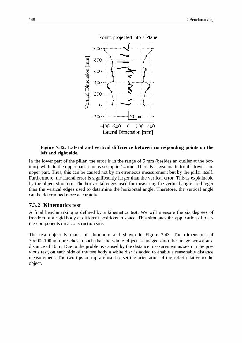
148 7 Benchmarking

Figure 7.42: Lateral and vertical difference between corresponding points on the left and right side.

In the lower part of the pillar, the error is in the range of 5 mm (besides an outlier at the bot-tom), while in the upper part it increases up to 14 mm. There is a systematic for the lower and upper part. Thus, this can be caused not by an erroneous measurement but by the pillar itself. Furthermore, the lateral error is significantly larger than the vertical error. This is explainable by the object structure. The horizontal edges used for measuring the vertical angle are bigger than the vertical edges used to determine the horizontal angle. Therefore, the vertical angle can be determined more accurately.

7.3.2 Kinematics test A final benchmarking is defined by a kinematics test. We will measure the six degrees of freedom of a rigid body at different positions in space. This simulates the application of plac-ing components on a construction site. The test object is made of aluminum and shown in Figure 7.43. The dimensions of 70×90×100 mm are chosen such that the whole object is imaged onto the image sensor at a distance of 10 m. Due to the problems caused by the distance measurement as seen in the pre-vious test, on each side of the test body a white disc is added to enable a reasonable distance measurement. The two tips on top are used to set the orientation of the robot relative to the object.

7.3 Application examples 149

a)

100 m

m

70 mm

90 m

m50 mm

b)

Figure 7.43: a) Schematic of the rigid body used in the measurement. b) Photo of the aluminum test body.

We note that the edges of the test body are somewhat rounded. Thus, the corner points are defined to an order of one tenth of a millimeter. The rigid body is mounted on a robot as shown in Figure 7.44 a). It is possible to shift and rotate the object with respect to the six degrees of freedom. The measurement configuration is shown in Figure 7.44 b), where the IATS is in the foreground and the robot in the back-ground. a) b)

Figure 7.44: a) Rigid body mounted on the robot. b) In front the theodolite with the robot behind.

The repeatability of the robot is specified as ± 0.1 mm. Additionally the error of measuring the orientation of the test body relative to the robot coordinate system must be considered. Experiments have shown that an absolute positioning accuracy in the order of ± 0.5 mm can be expected. To determine the six degrees of freedom of the object, the polar angles of several object points are measured and at least one point (disc) is determined in 3D (polar angles and dis-tance). These measurements are used to estimate the position and the rotation angles of the rigid body. The transformation is given by:

150 7 Benchmarking

0ii rr ⋅+= RT (7.2)

where ri0 Initial vector to an object point i at the rigid body R Rotation matrix. Combination of rotation around all three axes.

The rotation sequence is given by R = Rx(ω) ⋅ Ry(ϕ) ⋅ Rz(κ)

T Shift vector [x,y,z]T

The shift vector T and the rotation matrix R are known for each position from the robot posi-tioning. We will compare the results from the IATS measurement and the estimation with the reference data from the robot. The measurements are employed for ten distinct object positions at a distance between 10.188 m and 10.430 m. Images of the object at all positions are shown in Figure 7.45. a) b) c) d)

e) f) g) h)

i) j)

Figure 7.45: a)-j) Images of the rigid body at 10 different robot positions. We use the two-line-intersection method to measure the polar angles of corner points. The disc center is determined by disc matching yielding the polar angles. Additionally the distance is measured at the disc centers. The polar angles used in the estimation are derived from a two-face measurement to eliminate influences of the theodolite axis errors. Table 7.22 lists the difference of the shift vector (∆x, ∆y, ∆z) and the rotation angles (∆ω, ∆ϕ, ∆κ) between the reference data given by the robot and the measurements with the IATS. The last column denotes the number of corner points used in the position and orientation estima-tion.

7.4 Conclusions of the chapter 151

Station ∆x [mm]

∆y [mm]

∆z [mm]

∆ω [mgon]

∆ϕ [mgon]

∆κ [mgon]

# Points

1 -1.9 0.4 -0.8 -127.8 -298.1 -783.3 52 0.2 -0.1 -0.2 -275.9 -164.8 -168.5 63 0.2 -0.8 -0.4 -111.1 394.4 179.6 154 1.0 -0.3 -0.2 218.5 292.6 216.7 125 -1.0 1.1 0.0 100.0 218.5 296.3 156 -0.6 1.1 1.1 283.3 209.3 -357.4 127 0.7 -0.6 0.8 -51.9 316.7 -240.7 98 0.8 -0.9 -0.3 283.3 631.5 244.4 89 0.7 -0.6 -0.1 148.1 296.3 70.4 1510 0.2 -0.6 -0.9 -24.1 509.3 -35.2 10RMS 0.9 0.7 0.6 186.6 359.9 325.7

Table 7.22: Difference of the shift and the orientation between the robot data and the IATS measurement.

The RMS of the shift vector is below 1 mm in all three dimensions. Transforming the rotation error in a shift error considering the object length of 100 mm results in an error of 0.6 mm for 360 mgon. Thus, also the rotation error is below 1 mm. Considering the initial error of the robot positioning in the order of 0.5 mm, those results are very promising. [Aebischer & Braunecker, 2003] have shown, that the orientation of a coded circular cylinder recorded with a total station could be found with an RMS error of about 130 mgon (7 arcmin). Thus, the results with the IATS using a non-coded target are satisfactory.

7.4 Conclusions of the chapter The benchmarking tests discussed in this chapter have shown that it is possible to determine the polar angles of an object with the same precision as with a traditional total station. But at the same time those benchmarks have shown the weak points of the image-assisted approach. In the following we give a list of configurations leading to problems: • The distance measurement causes the main error in the 3D measurement. For several ob-

jects it is even not possible to measure the distance, e.g. copper roof of the Löwenhof. The reasons for the failure of the EDM are manifold: The angle of incidence of the laser on the object is far from 90°. Thus, the energy re-

turned to the receiver is too small for a correct distance measurement. The reflectivity of the object is poor, means it has a low albedo. This is the case for

dark objects. We have a multipathing situation, where parts of the laser spot are reflected from dif-

ferent surfaces. The result of the measurement is either a mix of all distances to the surfaces or a measurement error.

• Different illumination can change the visibility of an edge in the image so that it is not possible to extract the object boundary.

• The integration time of the image sensor is difficult to adjust when the illumination is not homogenous or if there is backlight.

• If the EDM is used for coarse focusing, the desired object to be measured must be in the center of the image otherwise the distance to a different object is measured for calculating the best focus position. Also, the contrast method can lead to focusing errors if multiple objects of different depths are in the field of view.

152 7 Benchmarking

• Dynamic objects such as vehicles or shadow from clouds can disturb the measurement. • It can happen that there is dirt on the lenses. This is difficult to detect and can produce

measurement errors. The MMI and the algorithmic processing are implemented on a desktop computer with Win-dows 2000 installed. The PC is placed on a trolley and situated besides the IATS, because they are wired for serial communication and for transmitting the image. Thus, the change from one position to the other took quite a long time. Further the PC need a 220V power sup-ply, which was solved by using two 12 V acid batteries and a transformer and is also not handy. But as already pointed out, this will not be the case if the IATS leaves prototype phase, where the MMI will be implemented on a palm computer or a tablet PC and the data are trans-ferred wireless. The handling of the IATS can be compared with the handling of a traditional total station. The objects to be measured are roughly aimed using the optical sight. Unfortunately, we cannot use the overview camera, because their vertical range is too small to capture the scene. This is a real disadvantage, because there are objects were a larger image of the surrounding would help to identify and select the correct object. Therefore, the overview camera must be redes-igned and fully integrated into the telescope. The placing of the approximation lines and the specification where to measure the distance using the graphical MMI is quite easy. It is also possible the assign a description and a num-ber to the object that is measured. The result of the measurement is displayed in a window, as well graphically as numerically. In case of multiple possibilities of lines describing the object, a dialog and a graphics are shown from where the correct one can be selected interactively. The handling of the interface was self explaining and easy. In average the measurement of a single point is in the range of 1 minute and 40 seconds. This is a summation of several different tasks, which are listed in Table 7.23. Task Time Coarse aiming the object: There are two ways of completing this task. Either the object is aimed using the optical sight or the image of the camera or a combination of both. It is possible to get the live image while the theodolite turns.

20-40 s

Selection of the target type and placing the approximation lines: Using the MMI the target type, e.g. “intersection of two lines” or “pole”, is specified and a description and a number are assigned to the object to be meas-ured. Further the approximation lines are placed and the position where to measure the distance specified using the actual image displayed.

20-30 s

Theodolite initialization: The theodolite is positioned as defined, the image integration time adjusted, the image grabbed and transferred to the PC, and finally the theodolite horizontal and vertical angles and the inclination angles are registered by the computer.

7 s

Algorithmic processing Detailed description of the computing performance can be found in sec-tion 5.2.5.

4-6 s

Interactive selection of the correct line if ambiguities occur 3-7 s

7.4 Conclusions of the chapter 153

Distance measurement: Theodolite is positioned to point to the object as defined for distance measure-ment and the distance is measured.

3-6 s

Online camera constant calibration: This is only needed, if the focus lens position has been changed since the last online calibration, otherwise the camera constant from the previous measure-ment can be used. As outlined in section 6.2 this will be replaced in a further development.

20 s

Table 7.23: Time consumption of the single tasks employed when measuring a sin-gle point.

Potential of reducing the time employed for a single point measurement can be seen in the multiple selection of object points within a overview image and in the elimination of the online camera constant calibration. The selection of the target type and the placing of the ap-proximation lines contains also potential for time reducing. The algorithmic processing takes only a small part of the overall time used for a single point measure. Future developments should address those problems.

8 Summary, conclusions and outlook

8.1 Summary In this thesis I present the development and the calibration of a prototype of an ‘Image As-sisted Total Station’ IATS, based on a modification of a Leica TPS 1100 Professional Series Total Station. The main goal of an IATS is to measure the 3D coordinates of non-cooperative but structured targets. The development work includes the concept layout, the hardware modi-fications, the implementation of new calibration routines and measurement algorithms and finally the benchmarking to outline the capability, but also the limits of this new system. In the following we summarize the main results of the thesis, as presented in the single chapters. Measurement concept The measurement concept of the IATS is based on a permanent interaction between the user and the instrument. This ‘hybrid’ mode will lead to a higher measurement efficiency that doubtless improves the user productivity. The user still has to select the object manually, has to define the measurement field of view and permanently controls the reliability of the results, while the instrument completes the routine work of the fine aiming and the measuring se-quence. Prototype The most important hardware modification is the integration of a coaxial looking CCD sensor with autofocus capability into the theodolite. The image data are transferred to a PC using a synchronized frame grabber. Different autofocus algorithms are examined and the one best suited for the IATS operation is selected. It is a combination of a direct distance measurement performed by the range finder, with a contrast maximization method based on a Sobel filter algorithm. Any hardware modification inside a mechanically optimized total station is risky and may lead to pointing errors, especially due to unavoidable thermal gradients in the warm-up phase. Tests were therefore undertaken to check the mechanical stability of the CCD mount, the exact linear movement of the motorized focus lens and the stress free installation of the limit switch. After switching-on the CCD, pointing errors of maximal 0.4 mgon are observed, which disappeared after one hour of operating keeping the pointing stability within the specifications. This drift has no influence on the benchmarking results where the theodolite is operated in a steady state. But these initial drifts observed must be eliminated by constructional means when going to production. Modeling An IATS is similar to a video theodolite and thus combines the typical features of a normal theodolite and a small angle photogrammetric camera. Analyzing the optical subsystem in its imaging properties shows that a pinhole model can be used to describe the overall imaging process, which allows to explain e.g. defocus phenomena. The model has to take into account all known error sources like those of the theodolite axes. The main part of this chapter de-scribes the transformation of a point on the sensor plane back to the object space. The chapter ends with a discussion of the accuracy needs for the focus lens positioning, and how the accu-racies of all sensors involved, like angle, tilt, distance, image processing, etc., contribute to the final measurement error. It becomes apparent that the main contribution to the error budget results from the ‘reflectorless’ range finder.

156 8 Summary, conclusions and outlook

Measurement algorithms Objects of different shape and structure will be measured by the IATS. In this thesis we con-centrate on objects of relatively high structural complexity, which can be sufficiently well approximated by geometrical ‘primitive’ structures. The algorithmic work is then reduced to find the best position and orientation match between the real object structure and its virtual ‘primitive’ counterpart. The algorithms are flexible enough to operate on a wide variety of object structures. The measurement sequence is as follows: After the object identification, a rough localization with pixel accuracy is performed based on an edge detection algorithm. This is followed by the localization routine using least squares matching algorithms and the back-transformation with sub-pixel accuracy. The results are the polar viewing angles of the object. Finally the object distance is measured to complete the 3D object coordinates. These procedures are cur-rently implemented for discs, for object points defined by an intersection of two lines or by tangents, for poles and also for the center of a prism plate. Calibration The IATS must be calibrated like any other theodolite, too. But since the visual path for direct observation is eliminated, the standard calibration concepts have to be revised, now including the CCD-camera and the focus encoder. We chose the following process: First the line of sight stability over temperature is measured, which delivers angular correction terms. Then the camera constant c depending on the opto-mechanical parameters is calculated. These pa-rameters vary when changing the focus. Since the accuracy achieved for c is not sufficient to fulfill the specifications needed, a newly developed ‘on-line’ calibration routine has to be per-formed at any focus lens position. Finally the mapping parameters for the back-transformation are determined by a scanning approach. The results indicate that the accuracy to localize an object in the image plane is about one tenth of a pixel, which corresponds to 0.25 mgon for a pixel size of 9 µm and a focal length of 228 mm. Benchmarking The benchmarking section is divided into three main parts: first measuring on known circular reference markers, secondly measuring on non-cooperative, but structured targets and third performing two realistic field applications. The measurements on the circular markers show an angular accuracy below 0.4 mgon. The overall positioning accuracy of about 3 mm is mainly limited by the distance measurement. The second test on non-cooperative targets is done with true objects. The accuracy obtained depends on the object and reaches from several millimeters up to 30 mm. The two field applications demonstrate the benefits, but also outline the limits of the IATS in practice. First, different objects like ‘capitals’, ‘volutes’ and ‘win-dow friezes’ on the facade of the historic ‘Löwenhof’ palace in Rheineck / Switzerland could be localized with a positioning accuracy of maximal 10 mm, depending on the illumination conditions and again on the rangefinder results. Finally a kinematical test is undertaken to determine the six degrees of freedom (6DoF) of a rigid body mounted on a robot drive, about 10 m away from the IATS. Here we found a position error of about 1 mm and an orientation error smaller than 360 mgon with respect to the robot coordinate system, which correspond to theoretical expectations. Presentations Parts of this thesis were presented, however in a rather early state, at the ‘6th Conference on Optical 3-D Measurement Techniques’ in Zurich 2003 [Walser & Braunecker, 2003].

8.2 Conclusions 157

8.2 Conclusions The results of this thesis work emphasize that the traditional high end total station, operated visually by an experienced geodetic engineer, can be substituted by a ‘pseudo-digital’ system where the coaxial looking eyepiece is replaced by a digital sensor. The classically achieved high performance is based on the human capability to interpret sceneries, even for point-like measurements. Thus our IATS solution tries to copy this process by sharing the task between the expert and the semi-automated system according to their inherent strengths: the capability of the user to distinguish between relevant and irrelevant conditions and the instrument's powerful and reliable detection mode for well defined object structures. The received point resolution of a tenth of a pixel, which is more or less the same as in the classical method, en-courages us to regard the IATS as successful demonstrator of a ‘Digital Total Station’.

8.3 Outlook Future work must be directed towards improving the hardware and software of this demon-strator. The current hardware components are commercially available add-on parts and must be properly selected and integrated on system level when going to production. The same holds for the software and the algorithms. The feedback from the application side is needed to decide about the final hardware and software layouts of a series model.

8.3.1 Software The current software implementation can handle only objects with linear boundaries. The measurement of few object points should be mostly sufficient to reconstruct the full object in 3D. Thus the possibility to match the measurement data e.g. with a CAD model of the object should be implemented as next step. Further, the instrument should also be capable to track incomplete structures like edges, if the object is only partially visible. This would enable the automatically measurement of more complicated structured objects. Introducing more sophisticated image recognition algorithms can obviously increase the de-gree of automation. The relation between user guidance and automatic task execution of the instrument can so favorably be shifted towards more automation. A great potential is seen by applying ‘knowledge-based system concepts’ as proposed by [Reiterer, Kahmen, Egly & Eiter, 2003b] or at least by integrating CAD data into the IATS similar to the work of [Streilein, 1999], from which the relevant measurement points are de-rived. Furthermore the virtual object can be layed over the image of the real object to visual-ize the matching quality. Another interesting point is the processing of spectral information [Niessner, 2003], an important information to characterize and extract special objects to ana-lyze e.g. their deformation.

8.3.2 Hardware The hardware improvement concerns not only the components like the sensor, but also their integration into the mechanical housing, the heat management and the calibration routines. The elimination of the direct visual channel will have consequences for the optics, which must be redesigned. The benchmarking experiments identified the ‘reflectorless’ range finder as main contributor, which limits the accuracy. We propose for improvement to integrate a micro-scanner in the IATS, which steers the ranging laser beam to any desired position within the field of view. The laser beam can then be directed to spots located close to the contour of the selected tem-plates. This additional local information leads to an overall better determination of the contour

158 8 Summary, conclusions and outlook

position and orientation. Furthermore the laser can be swept to areas of missing objects points to stabilize the overall object reconstruction. Due to the variable and fast pointing pos-sibility of the laser beam one can measure quasi-simultaneously several objects. Thus the use of a micro-scanner, which in its functionality is well known as fine pointing device in many optical free space communication instruments, will considerably increase the overall flexibil-ity and the operating speed of the IATS and will finally lead to a more reliable distance in-formation from the range finder. To add a small wide-angle camera helps to acquire more easily the objects. The camera should be integrated into the telescope body, looking into the same direction as the small-angle IATS sensor. A coaxial integration is not necessary, since the resulting parallactic errors can be mostly ignored in the acquisition mode and if required, can be easily corrected. Currently a PC operates the IATS and controls the image display. Later the computer and the display, preferably in color, must be integrated in the instrument.

8.3.3 Specifications of an IATS In the following we try to specify more quantitatively the IATS, based on the experience gained with the prototype. Baseline of our consideration is that all the performance data of traditional total stations must be maintained like the accuracy of the polar angle measure-ments with 0.3 mgon and of the tilt angle sensor with 0.2 mgon. Also the positioning speed of typical 50 gon/sec must be kept. The weight, the size, the power consumption, the operating and storage temperature range, all environmental tests, the integration into the mechanical theodolite structure, etc, all these features must be kept due to compatibility reasons with for-mer models. However some variations are recommended: • The measurement field of view should be variable between 1.7 gon and about 5 gon, cor-

responding to a maximum field of view of 2.4 m squared at an object distance of 30 m. It is then easier to identify and measure several objects in the field of view.

• The measurement rate for a dynamic measurement mode, means measuring the same ob-ject repeatedly, without distance measurement should be below 1 sec.

• The micro-scanner should be capable to address 10 positions randomly distributed in the field of view within 1 sec. In case of points located on a regular grid, the scan rate should be increased to about 100 points per sec.

When using the IATS to measure and track the 6DoF of a rigid object, which might be fixed on larger bodies, some requirements for the object size, structure, texture, etc would facilitate the work: • In dynamical applications the complete object or at least parts with sufficient information

like boundary lines should be visible inside the field of view. • The objects ideally should possess good visible edges that can be easily identified. Instead

of these structures also textures or even barcode pattern might be foreseen. • In order to get more reliable distance values by the range finder measurement, it is advan-

tageous to use objects with a planar patch from which the laser is reflected. Objects with rough surfaces are not well suited for the ‘reflectorless’ EDM.

8.3.4 IATS Applications The IATS is defined as upgrade of the traditional total station to measure single points with more reliability. Besides this the IATS offers more and new possibilities. In this section we

8.3 Outlook 159

will first comment the differences to scanners and photogrammetric cameras to outline appli-cations fields being unique for the IATS. Finally we will show special applications where the IATS can replace existing surveying systems. There is a wide variety of application fields where an IATS shows noticeable advantages compared to either classical theodolites or to competitive systems like photogrammetric cam-eras or laser scanners. IATS offers • A much higher pointing precision compared to laser scanning systems:

The angular accuracy of Total Stations like the TPS 1100 Professional Series is specified with 0.5 mgon, where e.g. the Cyrax HDS3000 high speed scanner is specified with 3.8 mgon and the Riegl LMS-Z360i with 2.8 mgon. The IATS operates therefore by a fac-tor 5 to 7 more precise.

• A better economy of sales: The IATS measures only points or structures with user defined relevance and must not collect those huge amounts of ‘data point clouds’ as laser scanners have to do when ana-lyzing unknown sceneries. Therefore IATS does not need extensive data handling and data storage means.

• An immediate availability of the results: Scanning and photogrammetric surveys need time intensive post-processing work to ex-tract the relevant data out of the data cloud or pictures, while the IATS measurement re-sults are immediately present, since the relevance selection is done when defining the ob-ject.

• A good depth perception: The combination of image processing with the point-wise distance measurements, which will be adaptively guided by the micro-scanner, allows dynamically performed 6DoF measurements of rigid objects without changing the instrument position.

Further IATS advantages are: • The IATS as total station is motorized and therefore allows tracking of objects moving out

of the instantaneous field of view. • The autofocus option gives the possibility to permanently focus on those object details,

describing best its position and orientation. Especially in industrial measurement applica-tions, where the object can carry a barcode, the autofocus option allows a large working volume in which the object can move.

• The IATS is much smaller and lighter than modern scanners of comparable performance, a significant advantage in daily work. The weight of the laser scanner Cyrax HDS2500 is about 15 kg, while that of total stations is about 5 - 7 kg.

• The power consumption of the Cyrax scanner is about 60-80 W, while total stations need about 5-7 W. Thus the IATS does not need the large and heavy acid batteries as laser scanners do. However, when increasing the computing power, inserting micro-scanners and adding more sensors for wide-angle optics will doubtless need more power. We esti-mated about 10 to 12 W.

We should also mention IATS related weaknesses: • The dependence on the correct definition of the object structure. This can be solved by a

better understanding and a more appropriate modeling of the object shape; by using more efficient algorithms for e.g. scale, position and rotation invariant object recognition in a pre phase.

160 8 Summary, conclusions and outlook

• The sensitivity to bad illumination profiles. Here we think to introduce an active, but cost reduced illumination set as being now installed in Leica industrial trackers.

• The limited accuracy of the range finder. As improvement we mentioned to perform rang-ing with the micro-scanner in case of natural sceneries. For tracking rigid bodies with a-priori known topology for general 6DoF applications, we mentioned as simple, but effec-tive improvements the use of planar patches for better beam reflection. Other possibilities are the installation of small retro-reflectors like in Leica T-probe scanners.

Industrial metrology Industrial metrology is in general an interesting application field of growing importance. The environmental conditions are well defined and the illumination profile can be adapted to the object structure. Since the objects are known from construction, the optimal templates to match their shape can be defined in advance and stored in the IATS databank. CAD data can also be used to drive the measurements and to compare permanently the degree of coinci-dence of the actual with the theoretical data. Construction Extending the idea of kinematical measurements will lead to general dynamic tracking appli-cations. After the object is identified, the IATS locks on and determines the actual position and orientation data. This will be done with rather coarse accuracy during track and with the required high accuracy when approaching the final destination. This dynamic mode is ex-tremely useful on large building sites, where prefabricated elements have to be placed. The instrument can track, measure and guide the total laying of these components. However, the current rather small field of view allows only small object sizes. We proposed to increase the field of view to 5 gon, since then the size of object details with sufficient information could be up to 2.4 m at a distance of 30 m. Another possibility is to perform the track with the wide-angle camera, but use the high resolution small field of view sensor to guide to the final posi-tioning. Deformation analysis Deformations of objects can be well analyzed by the IATS. The system “knows” the objects either from an initial measurement or from stored data like from CAD data bases. Due to the micro-scanner option multiple points can easily be measured in depth and angle. An update rate of the measurements for a single point of 1 Hz is desirable. If the objects are larger than the measurement field of view, the IATS will scan across the object with a maximal speed of 50 gon/sec. Forensic cases Further applications concern forensic cases, where contact-free measurements are indispensa-ble. Dedicated applications To conclude this section, we show some applications, where the IATS can replace or com-plement other surveying systems. Lots of those applications can be found in [Gruen & Kah-men, 2003]. • Traditional close range photogrammetry techniques and scanning systems need to set con-

trol points around the objects to be measured, using them as reference points to merge ad-jacent object field of views to a large observation field. It is well known that the setting of real control points is a very time consuming and labor intensive job. IATS can select and measure any structured object as virtual control point.

8.3 Outlook 161

• Many tasks require measuring the position of hidden points or of points inside tubes or cavities. By measuring the position and the orientation of a pivot point at the pointer stick and knowing the geometry of the stick allows to calculate the coordinates of its end point, where it touches e.g. the hidden surface point. This task is easily performable by the IATS. The image based calculations yield both polar angles and the ranging micro-scanner measures the distance to at least two sticker points. Applications are to obtain the depth of water holes or on construction sites to get the details behind larger components. Currently the hidden point measurements require a stick with two or three reflecting prisms. Then the stick must be kept motionless, while the TS measures sequentially to the prisms. The IATS implementation with micro-scanner allows shortening the measurement time by a factor about 5 to 10.

• Structural deformation monitoring is typically undertaken using sparse point-wise obser-vation techniques. These include contact sensors (e.g. dial gauges, LVDTs) and non-contact methods (e.g. theodolite intersection, close-range photogrammetry). IATS is a powerful alternative to these traditional sensors. An example of such a measurement is the controlled loading of a timber beam. It is easy to find planar patches there to facilitate the distance measurement. Furthermore, these objects offer enough edge structure to get re-liably the polar angles by image analysis. It would also be advantageous to add some markers, similar as done in photogrammetry.

• Another interesting possibility is the deformation monitoring of a complicated structure during its construction phase. A recent example is the measurement of the North Atrium of Federation Square in Melbourne, which consists of galvanized structural frames in tri-angular geometry, developed into a folded 3D structure that is glazed on the inside. Automated close-range photogrammetry is applied so far to provide comprehensive, high-accuracy 3D deformation data. Employing IATS would be an efficient alternative, be-cause the measurement points are well defined by the structure and the structural frame offers enough planar patches for accurate distance measurements.

• A rather special application for IATS is the gait analysis. To fulfill the high speed de-mand, the IATS tracks the person and measures the distance to only some characteristi-cally points, but saves the complete images. These are later evaluated for the polar angle determination.

• Building reconstruction is mostly done using close-range photogrammetry or laser scan-ning. But IATS could be a complementary instrument to complete this task. Thus, the IATS is not intended to replace, but to complement the ‘basket’ of surveying equipment.

Bibliography Ackermann, F., 1984. High Precision Digital Image Correlation. In Proceedings of the 39th

Photogrammetric Week, volume 9 of Schriftenreihe der Universität Stuttgart, Stuttgart. Aebischer, B. & Braunecker, B., 2003. Total Station for Measuring the 3-D Position and Ori-

entation of a rigid Body. Proceedings of 6th Conference on Optical 3-D Measurement Techniques, Zürich. Eds. Grün/Kahmen, Vol. I, pages 199 – 204.

Anai, T. & Chikatsu, H., 2000. Dynamic Analysis Of Human Motion Using Hybrid Video Theodolite. IAPRS, Vol. XXXIII; Amsterdam.

Baltsavias, E.P., 1991. Multiphoto Geometrically Constraint Matching. Mitteilungen Nr. 49, Institute of Geodesy & Photogrammetry, ETH-Zürich, Switzerland.

Bayer, H. A., 1987. Some Aspects of the Geometric Calibration of CCD-Cameras. ISPRS Conference on “Fast Processing of Photogrammetric Data”, Interlaken, June 2-4.

Bayer, H. A., 1992. Geometric and Radiometric Analysis of a CCD-Camera Based Photo-grammetric Close-Range System, Dissertation, Institute of Geodesy and Photogram-metry ETH Zurich, May 1992.

Blessing, P., 2000. Digitale Autofokus- und Beleuchtungskontrolle in der Endoskopie. Disser-tation der ETH Zürich, Diss. ETH Nr. 13615.

Brandstätter, G., 1989. Das analytische Modell der videogestützten räumlichen Zielerfassung mit panfokalem Fernrohr. Proceedings of first Conference on Optical 3-D Measurement Techniques Congress in Vienna/Austria. Eds Grün/Kahmen. Wichmann Verlag.

Brown, D.C., 1971. Close-Range Camera Calibration. Photogrammetric Engineering, 37 (8), pp. 855-866.

Burkhardt, H., 1999. Bildverarbeitungspraktikum. Albert-Ludwig-Universität, Freiburg, Insti-tut für Informatik.

Canny, J.F., 1986. A Computational Approach to Edge Detection. IEEE Transactions on Pat-tern Analysis and Machine Intelligence, 8(6):679-698.

Carosio, A., 1998. Fehlertheorie und Ausgleichsrechnung, Band 1. Auflage Oktober 1998. ETH Zürich, Departement Geodätische Wissenschafte.

Castleman, K. R., 1996. Digital Image Processing. Prentice-Hall, Inc. Chikatsu, H. & Anai, T., 2000. Development Of Hybrid Video Theodolite And Application

for 3D Modeling of Panoramic Objects. IAPRS, Vol. XXXIII; Amsterdam. Deumlich, F. & Staiger, R., 2002. Instrumentenkunde der Vermessungstechnik. 9., völlig neu

bearbeitete und erweiterte Auflage, Herbert Wichmann Verlag, Heidelberg. Dzierzega, A & Scherrer, R., 2003. Measuring with Electronic Total Stations. Survey Review,

Januray 2003, Vol. 37, No. 287. Dzierzega, A., 1986. DIOR 3002, Distanzmesser für Distanzmessung mit und ohne Reflektor.

Referet für die 7. Arbeitssitzung der ISM-Kommission 3 in Siofok, Ungarn. EPSIC, undated. Les systèmes autofocus, Ecole professionnelle de Lausanne, Technologies

Audio et Vidéo. http://www.epsic.ch/Branches/audiovideo/video/autofocus-1.html. Fabiankowitsch, J., 1990. Automatische Richtungsmessung mit digitalen Differenzbildern.

Dissertation, TU Wien. Faulhaber Group, 2000. Motion Controller, 4-Quadrant PWM for DC-Micromotors, MCDC

2805 Series, Operating Instructions. Edition 24.08.2000. Finsterwalder, R. & Hofmann, W., 1968. Photogrammetrie. 3rd edition. Walter de Gruyter &

Co, Berlin 1968.

164 Bibliography

Förstner, W. & Gülch, E., 1987. A Fast Operator for Detection and Precise Location of Dis-tinct Points, Corners and Centers of Circular Features. ISPRS International Workshop, Interlaken, June, 281-305.

Gong, D., Huang, Y. D. & Ball, S. L., undated. A Laser Scanning Videotheodolite For 3D Visualisation and Metrology. http://www.alphageofisica.com.br/mdl/06video.pdf

Gottwald, R., 1987. Kern E2-SE – Ein neues Instrument nicht nur für die Industrievermes-sung? AVN, Heft 4, S. 147 – 153.

Gruen, A. & Huang, T. S., 2001. Calibration and Orientation of Cameras in Computer Vision. Springer Verlag.

Gruen, A. & Kahmen, H., 2003. Proceedings of 6th Conference on Optical 3-D Measurement Techniques, Zürich. Vol. I & II

Gruen, A. & Stallmann, D., 1993. High accuracy edge matching with an extension of the MPGC-matching algorithm. Applications of Geodesy to Engineering, IAG Symposia, Vol. 108, Springer Verlag, pp. 339-350.

Gruen, A., 1985. Adaptive Least Squares Correlation – A Powerful Image Matching Tech-nique. South African Journal of Photogrammetry, Remote Sensing and Cartography, 14 (3), pp. 175-187.

Gruen, A., 1992. Machine Vision – Elitärer Forschungsgegenstand oder ein neues interessan-tes Arbeitsgebiet auch für den praktizierenden Vermessungsingenieur? AVN, Heft 8-9, S. 321-324.

Gruen. A, & Agouris P., 1994. Linear Feature Extraction by Least Squares Template Match-ing Constrained by Internal Shape Forces. International Archives of Photogrammetry and Remote Sensing, Vol. XXX, Part 3/1, pp. 316-323. Presented at the ISPRS Com-mission III Symposium in Munich, Germany, September 1994.

Gülch, E., 1994. Erzeugung digitaler Geländemodelle durch automatische Bildzuordnung. PhD thesis, Institute of Photogrammetry, University of Stuttgart. Deutsche Geodätische Kommission Vol. 418.

Haralick, R. M. & Shapiro, L. G., 1992. Computer and Robot Vision, Volume II, Addison-Wesley, pp. 316-317.

Haralick, R. M., 1984. Digital Step Edge from Zero Crossings of Second Derivative. IEEE Transactions on Pattern Analysis and Machine Intelligence, 6(1): 58-68.

Hecht, E., 2002. Optics. Fourth Edition, Addison Wesley, New York. Heipke, C., 1996. Overview of Image Matching Techniques. Proceedings of the OEEPE

Workshop on the Application of Digital Photogrammetric Workstations. March 4-6, Lausanne, Switzerland. http://dgrwww.epfl.ch/PHOT/workshop/wks96/art_3_1.html.

Heitger, F., 1995. Feature Detection using Suppression and Enhancement. Technical Report TR-163, Image Science Lab, ETH-Zurich, Switzerland.

Henricsson O., 1996. Analysis of Image Structure using Color Attributes and Similarity Rela-tions. Ph.D. Thesis, Report No. 59, Institute of Geodesy and Photogrammetry, ETH Zu-rich, Switzerland.

Höpcke, W., 1980. Fehlerlehre und Ausgleichsrechnung. Walter de Gruyter Verlag, Berlin. Horn, B.K.P.; 2000. Tsai’s Camera Calibration Method Revisited.

http://www.ai.mit.edu/people/bkph/papers/tsaiexplain.pdf Hovenbitzer, M. & Schlemmer, H., 1997. A Line-Scanning Theodolite-Based System for 3D

Applications in Close Range. Proceedings of 4th Conference on Optical 3-D Measure-ment Techniques, Zurich/Switzerland. Eds. Grün/Kahmen, Wichmann Verlag, pages 339–345.

Huang, Y. D., 1992. 3-D Measuring System Based on Theodolite-CCD Cameras. XVIIth ISPRS-Congress. Volume XXIX. Commission V. Part B5. Washington D.C. p. 541-544.

Bibliography 165

Huang, Y.D. & Harley, I., 1989. Calibration of Close-Range Photogrammetric Stations Using a Free Network Bundle Adjustment. Proceedings of first Conference on Optical 3-D Measurement Techniques, Vienna/Austria. Eds. Grün/Kahmen Wichmann Verlag.

Huep, W., 1988. Konzeption und Einsatzmöglichkeiten eines automatisierten Theodolit-systems. X. Internationaler Kurs für Ingenieurvermessung, September 1988, München, S. A13/1-A13/13.

ISO 17123-3, 2001. Optics and optical instruments − Field procedures for testing geodetic and surveying instruments − Part 3: Theodolites. First edition, 2001-12-01. ISO copyright office.

Julien, P., 1999. Principles of digital matching. Proceedings of the OEEPE Workshop on Automation in Digital Photogrammetric Production. Marne la Valeé, 22-24 June 1999, Ecole Nationale des Sciences Géographiques.

Juretzko, M., 2001. The System TOTAL for Recording Geometry and Image Data of Historic Buildings and Monuments. CIPA International Symposium, Potsdam.

Kahmen, H. & de Seixas, A., 1999a. Object Recognition with Video-Theodolites and without targeting the Object. Proceedings of the IWAA, 6th International Workshop on Align-ment Accelerator. Grenoble, France.

Kahmen, H. & de Seixas, A., 1999b. 3D Object Sensing with Computer controlled rotating CCD Cameras. XVII Cipa International Symposium, Recife, PE-Brasil.

Kahmen, H. & de Seixas, A., 2000. Neue Theodolitmessverfahren für die Bestimmung von Deformationen an nicht signalisierten Objekten. XIII. International Course on Engineer-ing Surveying. Munich.

Kahmen, H. & Roic, M., 1995. A New Generation of Measurement Robots for Object Recon-struction without Targeting. Proceedings of 3rd Conference on Optical 3-D Measure-ment Techniques, Vienna/Austria. Eds. Grün/Kahmen, Wichmann Verlag, pages 251 – 262.

Kahmen, H., Niessner, A. & de Seixas, A., 2001a. 3D Object Sensing Using Rotating CCD Cameras. Kropatsch, W.G., Bishof, H. (Eds.): Digital Image Analysis. Springer Verlag, Berlin.

Kahmen, H., Niessner, A. & de Seixas, A., 2001b. On-Line Deformation Measurements with Rotating Computer Controlled CCD Cameras. Proceedings of 5th Conference on Opti-cal 3-D Measurement Techniques, Vienna/Austria. Eds. Grün/Kahmen, Wichmann Ver-lag, pages 389 – 396.

Kahmen, H., 1998. Advances in Metrology with a new Generation of Measurement Robots. XXI International Congress FIG, Brighton, United Kingdom.

Kahmen, H., 2001. Knowledge Based 3 D Measurement Systems with Rotating Cameras. Fourth International Symposium “Turkish - German Joint Geodetic Days”, Berlin, April 2001.

Kessler, W. & Fischer, J., 2000. Analytical model of autofocus systems with CCD cameras. Proceedings of SPIE, Sensors and Camera Systems for Scientific, Industrial, and Digital Photography Applications, Volume 3965. 24-26 January 2000, San Jose, USA.

Koch, K.R., 1999. Parameter Estimation and Hypothesis Testing in Linear Models. Springer Verlag, Berlin Heidelberg.

Kraus, K., 1997. Photogrammetrie, Band 1, Grundlagen und Standardverfahren. 6. Auflage, Dümmler Verlag, Bonn.

Krauth, A. & Wrobel, B., 1993. Target localization by least squares image matching including the deconvolution of image blur. Proceedings of 2nd Conference on Optical 3-D Meas-urement Techniques, Zurich/Switzerland. Eds. Grün/Kahmen, Wichmann Verlag.

Leica Geosystems AG, 2000. GeoCOM Reference Manual, TPS1100 - Version 1.07. Leica Geosystems AG, 2002. Leica TPS1000 Professional Series – Technical Data.

166 Bibliography

Leica Geosystems AG, 2003. Leica TPS1000 Professional Series – User Manual, Version 2.2. Lewis, J. P., 1995. Fast normalized cross-correlation. Online, Internet, Available:

www.idiom.com/~zilla/Work/nvisionInterface/nip.pdf Liao, B., 1993. Ein Beitrag zur Kamerafokussierung bei verschiedenen Anwendungen der

Bildverarbeitung. Dissertation im Fachbereich Maschinenbau der Universität der Bun-deswehr Hamburg.

Luhmann, T., 2000. Nahbereichsphotogrammetrie. Lehrbuch, Wichmann Verlag, Heidelberg. Maas, H.-G., Nideröst, M., 1997. The accuracy potential of large format stillvideo cameras.

Videometrics V, SPIE Proceedings Series Vol. 3174, SPIE’s 42nd Annual Meeting, San Diege.

Marr, D. & Hildreth, E., 1980. Theory of edge detection. Proceedings of the Royal Society of London, B 207: 187−217.

Mason, S., 1994. SGAP: Batch Program for Bundle Adjustment Processing, Documentation and Users Guide, Institute for Geodesy and Photogrammetry ETH-Zurich, December 1994.

Matrox, 1996. Matrox Image Tutorial, Camera Interface Guide. Matrox Electronic Systems, Ltd. Printed in Canada, 01-11-1996, Rev.: $IE-4648-B.

Matrox, 2001. Matrox Meteor-II / Multi-Channel, Installation and Hardware Reference. Man-ual no. 10761-101-0101. October 29, 2001.

Mischke, A. & Kahmen, H., 1997. A New Kind of Measurement Robot System for Surveying on Non Signalized Targets. Proceedings of 4th Conference on Optical 3-D Measure-ment Techniques, Zurich/Switzerland. Eds. Grün/Kahmen, Wichmann Verlag, pages 311–318.

Mischke, A & Wieser, A., 1995. Automatic Target-Area-Collimation with Video-Theodlites. Proceedings of 3rd Conference on Optical 3-D Measurement Techniques, Vi-enna/Austria. Eds. Grün/Kahmen, Wichmann Verlag, pages 263 – 271.

Mischke, A., 1996. Distanzmessung mittels Autofokusfunktion einer CCD-Kamera. AVN, Heft 1, pages 31 – 39.

Mischke, A., 2000. Entwicklung eines Videotheodolit-Messsystems zur automatischen Rich-tungsmessung von nicht signalisierten Objektpunkten. Geowissenschaftliche Mitteilun-gen, Heft 54. Wien.

Neumann, H. & Schröder, G., 1992. Bauelement der Optik, Taschenbuch der technischen Optik. 6. neubearbeitete Auflage. Carl Hanser Verlag München Wien.

Niessner, A., 2003. Qualitative Deformationsanalyse unter Ausnutzung der Farbinformation. Geowissenschaftliche Mitteilungen, Heft 63. TU Wien.

Pateraki, M., 2000. Image Matching Methods. Internal Report IGP - June 2000. Perona, P, & Malik, J., 1991. Detecting and localizing edges composed of steps, peaks and

roofs. In International Conference on Computer Vision, p. 52−57, Osaka, Japan. Reiterer, A., Kahmen, H., Egly, U. & Eiter, Th., 2003a. 3D-Vermessung mit Videotheodoliten

und automatisierte Zielpunkterfassung mit Hilfe von Interest Operatoren. Allgemeine Vermessungs-Nachrichten (AVN), 110 (2003), 04; 150 - 156.

Reiterer, A., Kahmen, H., Egly, U. & Eiter, Th, 2003b. Knowledge-Based Image Prepro-cessing for a Theodolit Measurement System. Proceedings of 6th Conference on Optical 3-D Measurement Techniques, Zürich. Eds. Grün/Kahmen, Vol. I, pages 183 - 190.

Riechmann, W., 1992. The Accuracy of the Réseau-Scanning Camera (RSC) in Comparison with Theodolite- and Photogrammetric Systems. ISPRS-Congress, Washington D.C. Vol. 29, B5, pages 852−586.

Roic, M., 1996. Erfassung von nicht signalisierten 3D-Strukturen mit Videotheodoliten. Ge-owissenschaftliche Mitteilungen, Heft 43. Wien.

Bibliography 167

Rottensteiner, F., 2001, Semi-automatic extraction of buildings based on hybrid adjustment using 3D surface models and management of building data in a TIS. Dissertation, TU Wien.

Scherer, M., 1995. Ein Expertensystem zur Architekturaufnahme - Bausteine auf dem Weg dorthin, Zeitschrift für Vermessungswesen ZfV, 3/1995, pp. 134–143.

Scherer, M., 2002. Advantages of the Integration of Image Processing and Direct Coordinate Measurement for Architectural Surveying –Development of the System Total. FIG XXII International Congress, Washington D.C. USA, April 19−26.

Seatovic, D., 2000. Integration eines motorisierten Videotheodoliten TM3000V in das Karls-ruher Industriemesssystems. Diplomarbeit, Karlsruhe.

Sony, 1999. Monochrome Card Camera: CCB-M Series – Component/OEM. Sony, undated. ICX055BL, Diagonal 6mm (Type 1/3) CCD Image Sensor for CCIR B/W

Video Cameras .Datasheet. Stöcker, H., 1995. Taschenbuch mathematischer Formeln und moderner Verfahren. 3. überar-

beitete und erweiterte Auflage, Verlag Harri Deutsch. Strang, G. & Borre, K., 1997. Linear Algebra, Geodesy, and GPS. Wellesley-Cambridge

Press. Streilein, A. 1999. Digitale Photogrammetrie und CAAD. Mitteilungen Nr. 68, Institute of

Geodäsie & Photogrammetrie, ETH-Zürich, Switzerland. Stuart, A., Ord, J. K. & Arnold, S., 1999. Kendalls’s Advanced Theory of Statistics. Classical

Inference & the Linear Model. Sixth Edition, Volume 2A. Torge, W., 2001. Geodesy. 3., completely rev. and extended ed. Berlin, New York, de

Gruyter. Uffenkamp, V., 1993. Conception of a digital turning and tilting camera. Proceedings of 2nd

Conference on Optical 3-D Measurement Techniques, Zurich/Switzerland. Eds. Grün/Kahmen, Wichmann Verlag, pages 72 – 80.

Uffenkamp, V., 1995. Konzeption, experimentelle Realisierung und Kalibrierung einer opto-elektronischen Schwenk-Neige-Kamera mit langer Brennweite. Dissertation, TU Mün-chen.

Wallis, R., 1976. An approach to the space variant restoration and enhancement of images. Proc. of Symposium on Current Mathematical Problems in Image Science, Naval Post-graduate School, Monterey, CA, November.

Walser, B. & Braunecker, B., 2003. Automation of Surveying Systems through Integration of Image Analysis Methods. Proceedings of 6th Conference on Optical 3-D Measurement Techniques, Zürich. Eds. Grün/Kahmen, Vol. I, pages 191 – 198.

Wasmeier, P., 2002. Potential der Objekterkennung mit dem Videotheodolit TCA2003. Dip-lomarbeit, TU München.

Weisstein, E.W., 2004. “Least Squares Fitting.” From MathWorld--A Wolfram Web Re-source. http://mathworld.wolfram.com/LeastSquaresFitting.html.

Wester-Ebbinghaus, W., 1985. Bündeltriangulation mit gemeinsamer Ausgleichung photo-grammetrischer und geodätischer Beobachtungen. Zeitschrift für Vermessungswesen, 110 (3), pp. 101-111.

Wester-Ebbinghaus, W., 1988a. High Resolution Object Recording by Video-Theodolite. ISPRS-Congress, Com. V, Kyoto 1988, Vol. 27, B10, pages 219−223.

Wester-Ebbinghaus, W., 1988b. Analytics in non-topographic Photogrammetry. ISPRS-Congress, Com. V, Kyoto 1988, Vol. 27, B11, pages 380−390.

Wieser, A., 1995. Ingenieurgeodätische Überwachungsmessung mit Videotheodoliten. Dip-lomarbeit, TU Wien.

Zeiske, K., 2000. Vermessen leicht gemacht. Leica Geosystems AG, Heerbrugg, Switzerland.

168 Bibliography

Zhang, Z., Zheng, S. & Zhan, Z., 2003. Photo Total Station System an Integration of Metric Digital Camera and Total Station. Proceedings of 6th Conference on Optical 3-D Meas-urement Techniques, Zürich. Eds. Grün/Kahmen, Vol. I, pages 176 – 182.

Ziou, D. & Tabbone, S., 1998. Edge Detection Techniques − An Overview. International Journal of Pattern Recognition and Image Analysis, Vol. 8, No. 4, pp. 537-559, 1998. also Technical Report, No. 195, Dept. Math. et Informatique, Université de Sherbrooke, 41 pages, 1997.

Acknowledgement I thank Prof. Dr. Armin Grün for giving me the opportunity to do this work at his research institute as external dissertation, for providing a lot of ideas and tips during my work and for being my examiner. I also thank my two co-examiners. I am grateful for the input of Prof. Dr. Herbert Kahmen. Moreover, I am indebted to Dr. Bernhard Braunecker for providing me an excellent research environment at Leica Geosystems AG, for serving as my supervisor, for all the fruitful discus-sions and for carefully reading and correcting the thesis. Many thanks go to Richard Wenk and Pius Vorburger for giving me the chance to accomplish the dissertation at Leica Geosystems AG. Special thanks also go to Dr. Bernhard Gächter for his inputs in the periodical meetings. An experimental project such as this requires a lot of support of a large number of persons. The help of colleagues and the employees of Leica Geosystems have been of invaluable throughout my work. I would also like to thank Dr. Jürg Weilenmann, Dr. Marcel Rohner and Dr. Beat Aebischer for reading and correcting my “Swiss English” and for the critical remarks. I further will thank the Institute of Geodesy and Photogrammetry from ETH Zurich for the opportunity to use software functions from the project AMOBE. I would also thank Dr. Holger Kirschner for his help and contributions to the development of the autofocus algorithms. My acknowledgements extend to my parents who have given me the opportunity to study and who have supported me throughout the many years of my studies. My wife Nadia and my children Miro and Shana have provided me with incessable support during this long period and has put up with me working for evenings and weekends.

Curriculum Vitae Personal Data Name: Bernd Hanspeter Walser Title: Dipl. El.-Ing. ETH Data of Birth: March 10, 1972 Place of Birth: St. Gallen, Switzerland Nationality: Swiss Formation 2000−2004:

Ph.D. student Institute of Geodesy and Photogrammetry (IGP) Swiss Federal Institute of Technology (ETH), Zurich, Switzerland Ph.D. Thesis: Development and Calibration of an Image Assisted Total Station Development engineer Leica Geosystems AG, Heerbrugg

1998−2000:

Development engineer Leica Geosystems AG, Heerbrugg

1992−1998:

M.Sc. in Electrical Engineering (Eidg. Dipl. El.-Ing. ETH) Swiss Federal Institute of Technology (ETH), Zurich, Switzerland Master Thesis: Distanzmessung und Datenübertragung mit einem Laser

1992:

Compulsory military service 1987−1992

High school graduation, type C Kantonsschule Heerbrugg, Switzerland

Languages

Native language: German Foreign languages: Englisch, French