1

Developing a Best Estimate of Annual Vehicle Mileage for 2017 NHTS Vehicles

1. Introduction

From the 2001 to the 2017 NHTS, the number of miles (VMT) driven by an

NHTS household vehicle can be estimated in three different ways. First, one can use the

single odometer reading1 to compute an estimate of annual mileage. Second, a designated

household member was asked to report the total number of miles driven in each of the

household vehicles (“self-reported VMT” or ANNMILES). Finally, the amount of annual

driving can be estimated based on the amount a vehicle is driven during the designated

sample day (i.e., the travel day). Ideally, annualizing the odometer readings would

probably generate the most reliable VMT estimate, as compared to estimates based on the

other two approaches. Unfortunately, not all vehicles had an odometer reading recorded.

Furthermore, of those that had their odometer reading recorded, the quality of some of the

reported odometer readings is less than desirable. As such, ORNL was asked to estimate

the number of miles driven by each of the NHTS vehicles based on the best available data

(i.e., BESTMILE). Note that BESTMILEs are computed only for automobiles, pickup

trucks, vans, and sport utility vehicles. For motorcycles, other trucks, and recreational

vehicles (RV), the BESTMILE is equal to the value of the self-reported VMT for those

vehicles with such information available.

As with every iteration of the NHTS, the 2017 version contained changes in

which variables were asked, and in how they were asked. The 2017 NHTS featured a

change in the way mileage was calculated for each trip taken on the travel day.

Specifically, in 2009, the survey respondent was asked to self-report the miles traveled

for each individual trip, while in 2017, the respondent provided origin and destination

locations from which trip mileage was computed using Google distance APIs. Because of

this, vehicle miles of travel (VMT) based on the trip day was methodologically different

from 2009 to 2017. This difference made it vital that other measures of miles traveled,

1 In the 2001 NHTS, two odometer readings were sought from the respondent.

2

such as self-reported miles driven in each household vehicle (“the “self-reported VMT”

or ANNMILES referred to earlier), as well as the miles per vehicle estimate based on the

best available data (namely, BESTMILE), be held as consistent as possible across the

survey iterations. Thus, the method used in computing BESTMILE for the 2017 NHTS,

as well as this documentation, borrowed extensively from the 2009 documentation,2 with

changes from the 2009 method highlighted and numbers updated as appropriate.

Another big change that impacted the estimation of BESTMILE for 2017 NHTS

was in how the survey collects information regarding the length of time a vehicle was

owned by the respondent. In past surveys, the NHTS asked how long a household owned

their vehicle for every vehicle, and allowing the response to be given in days, weeks,

months, or years. In the 2017 NHTS, respondents were only asked the number of months

the vehicle was owned, and only for vehicles owned for a year or less. This limitation

negatively impacted the estimation methodology applied in computing the BESTMILE

(see Section 3).

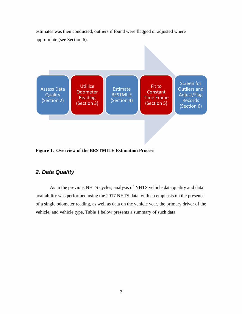
Aside from this limitation, on how long a vehicle was owned, the process of

estimating BESTMILE for vehicles in the 2017 NHTS followed what was done for the

2001 and 2009 surveys. The process, summarized in Figure 1 below, began with an initial

overview of data quality (see Section 2), which involved assessing the number of sample

vehicles that had necessary components for the BESTMILE estimation, such as an

odometer reading, vehicle year, and information on the primary driver. Next, an

investigation of how to best use the single odometer reading information was performed

(see Section 3), generally associated with adjusting for the lack of information on how

long the vehicle was owned by the household. Once that was accomplished, the

calculation of BESTMILE was performed (see Section 4). Finally, the initial

BESTMILE estimates were adjusted to fit a precise time frame - April 1, 2016 to March

31, 2017 (see Section 5). A screening process to identify potential outliers in the

2 Developing a Best Estimate of Annual Vehicle Mileage for 2009 NHTS Vehicles, included as part of the

Derived Variables documentation at https://nhts.ornl.gov/2009/pub/DerivedAddedVariables2009.pdf,

accessed June 15, 2018.

3

estimates was then conducted, outliers if found were flagged or adjusted where

appropriate (see Section 6).

Figure 1. Overview of the BESTMILE Estimation Process

2. Data Quality

As in the previous NHTS cycles, analysis of NHTS vehicle data quality and data

availability was performed using the 2017 NHTS data, with an emphasis on the presence

of a single odometer reading, as well as data on the vehicle year, the primary driver of the

vehicle, and vehicle type. Table 1 below presents a summary of such data.

Assess Data Quality

(Section 2)

Utiliize Odometer

Reading (Section 3)

Estimate BESTMILE (Section 4)

Fit to Constant

Time Frame (Section 5)

Screen for Outliers and Adjust/Flag

Records (Section 6)

4

Table 1. 2017 NHTS Vehicle Data Quality Checks

Data Quality Checks Sample Vehicles %

Total 2017 NHTS Vehicles 256,115 100.0%

No Odometer Reading 40,849 16.0%

No Vehicle Year 348 0.1%

No primary driver associated with the vehicle 3,059 1.2%

Out of Scope Vehicle Types3 8,988 3.5%

Vehicles without Data necessary for eventual BESTMILE estimation4

529 0.2%

Vehicles with Usable Odometer Data 202,342 79.0%

Vehicles with Presumed Odometer Rollovers5 5,279 2.1%

The percentage of vehicles with the complete set of needed odometer data

(odometer reading, vehicle year, primary driver, etc.), which the calculation of

BESTMILE was based on (at least in part), was 79.0%, a number far larger than the

63.9% in 2009. This increase in response was unexpected and may impact comparability

of BESTMILE estimates across surveys as more vehicles will be estimated with a

specific method than in the past. Table 2 summarizes the distribution of 2017 NHTS

vehicles in terms of key elements of data used to compute BESTMILE.

3 The out of scope vehicle types included “motorcycles,” “other trucks,” “recreational vehicles,” and

vehicles with missing vehicle type information. 4 This includes specific variables used in various regression models. For example, a vehicle may have

primary driver information, but not have a value for a specific variable, such as EDUC (Education of the

driver). Some of this was accounted for in the 2001 models; however, some variables may have specific

values in 2017 that are not present in 2001. 5 If a vehicle was at least 20 years old and the odometer reading was less than 100,000, analysis was

performed regarding a possible unrecorded odometer rollover. If adding 100,000 or 200,000 miles to the

odometer reading resulted in an average miles per year of less than the 75th percentile of miles per year for

vehicles, by age group, for those vehicles at least 20 years old with more than 100,000 miles, then the

additional 100,000 or 200,000 miles were added to the odometer reading. The 75th percentile cutoffs were

10,000 miles per year for 20-24 year old vehicles, 7,500 miles for 25-29 year old vehicles, 6,000 miles for

30-39 year old vehicles, and 4,000 miles for vehicles 40 years and older.

5

Table 2. NHTS Vehicles6 by Data Required for 2017 BESTMILE Estimation

Usable Data to Estimate Odometer-Based BESTMILE

Yes No

Usable Self-Reported VMT

Usable Self-Reported VMT

Yes No Yes No

Information on Primary Driver?

Information on Primary Driver?

Information on Primary Driver?

Yes Yes No Yes No

One driver/One vehicle HHs 31,103 174 2,877 195 119 22

Two drivers/two vehicles HHs 68,211 222 9,911 312 266 22

Other Drivers=Vehicles HHs 14,528 79 3,550 186 118 25

Drivers > Vehicles HHs 10,172 60 1,835 64 46 5

Drivers < Vehicles HHs 77,418 375 14,814 4,205 447 799

Subtotal 201,432 910 32,987 4,962 996 873

Subtotal by Usable Data 202,342 39,818

3. Initial Determination of An Annualized Odometer Estimate (ODOMMILES)

The 2009 BESTMILE estimates determined how to use a single odometer reading

instead of two via simple regression models based on vehicle age for vehicles purchased

new and used. In 2001 and 2009, since a question asking the respondent if they purchased

the vehicle new or used was not asked, for purposes of BESTMILE analysis, a vehicle

was considered purchased “used” if it was 2 or more years older (as determined through

the vehicle model year) than the amount of time it was owned by the household. In 2017,

this was complicated by the removal of the question “How long have you had the

[household vehicle]?” in all cases where a vehicle was owned by the household for longer

than a year. To compensate for the loss of this data item from 2017 NHTS, a logistic

regression model was developed for vehicles owned more than 12 months. This model

used data on vehicles and their assigned new/used status from 2009 as the dependent

variable, with independent variables including vehicle age, vehicle age squared, vehicle

6 There were 256,115 vehicles included in the 2017 NHTS survey. However, 13,955 of these vehicles were

out of scope for the BESTMILE estimate. The out of scope vehicle types included “motorcycles,” “other

trucks,” “recreational vehicles,” and vehicles with missing vehicle type information. BESTMILE for these

vehicles was set to the self-estimated annual miles driven, where available.

6

type, household income, urban/rural status, race of the household respondent, Census

region of the household, and where available, age and sex of the primary driver. The

probability �̂� that a vehicle would be assigned as new or used is described by Equation

(1):

�̂� =𝑒𝐵0+𝐵1𝑋

1+𝑒𝐵0+𝐵1𝑋 (1)

where B0 + B1X represents a linear equation with intercept B0 and the vector of

independent variables (detailed above) B1X. As hinted at above, two separate logistic

regressions were developed – one including primary driver characteristics, and one

without. The models predicted new/used status correctly 76.4% and 74.1% of the time,

respectively. With new vehicles totaling 61.8% and 61.2% of 2009 NHTS vehicles, and

the remainder assigned to used status, this improvement in prediction is better than

random chance, and adequate for randomly assigning new/used status to 2017 NHTS

vehicles in the absence of months owned data.

Once new/used status was assigned, the next step in simulating 2009 data for

vehicles in the 2017 dataset was to generate a months-owned value for each vehicle

owned more than 12 months. Different approaches were applied for new vehicles and

used vehicles. For new vehicles, months-owned was close to the age of the vehicle,

within an error of 24 months. To account for this error, the 2009 distribution of the

number of months a vehicle was owned by the household was determined for each

vehicle age, and a months-owned number was randomly assigned to each 2017 vehicle

assigned as a new vehicle. Since there was greater variability in months-owned for used

vehicles, a simple linear regression model, expressed in Equation (2), was formed:

𝑀𝑜𝑛𝑡ℎ𝑠 𝑂𝑤𝑛𝑒𝑑 = 𝛽0 + 𝛽1𝑋 (2)

where X is the same vector of independent variables used in Equation (1). After this step

was completed, the data available for vehicles in the 2017 set was now equivalent to

those of 2009 in terms of completeness. Thus, the method for computing both the

7

initialized odometer estimate (ODOMMILES) and BESTMILE was the same as in the

2009 documentation from this point forward.

Using data on self-reported miles driven by new/used status and vehicle age, three

regressions (one for new vehicles, one for used, and one for all vehicles – for use on

vehicles where new/used status is unknown) were run to determine the relationship

between vehicle age and annual miles driven. These three regressions, calculated

separately but taking the same form, are summarized by Equation (3)7:

2

21 )()( Miles Annual Reported-Self VehicleAgeVehicleAge ++= (3)

Predicted values for each regression were computed for each vehicle age, which

in the 2001 NHTS data ranges from 1 to 40. The predicted values by age are summarized

in Figure 2.

7 Note that regressions for 2001 and 2009, while taking the same form, were computed separately, leading

to slightly different parameter estimates between surveys. To minimize year-to-year differences, 2017

vehicles were computed using the 2009 model. Admittedly, for both 2001 and 2009, the R-squared values

of all models are low (in the .04-.07 range). However, all model terms and the models themselves are

statistically significant, and given the large amount of variation among vehicles in both surveys, one would

expect R-squared values to be somewhat low.

8

Figure 2. Average Self-Reported Miles (Smoothed via Regression Modeling) by

Vehicle Age and New/Used Status, 2001 NHTS National Sample Vehicles

For each vehicle in the NHTS data, these predicted values were used to determine

the percentage of travel that a given vehicle took in the most recent year, given the

vehicle age and its subsequent cumulative mileage. Equation 4 shows the mathematical

relationship of the percentage of the single odometer reading and the current year mileage

for new vehicles8:

=

=t

1i

i

t

i

Miles Reported Self Estimated

Miles Reported Self Estimated Percent Mileage New x 100% (4)

where t is the vehicle age, and the numbers for Estimated Self-Reported Miles are

estimated using the regression for new vehicles from Equation 3. This percentage is then

multiplied by the odometer reading to compute the estimated annual mileage

(ODOMMILES) in the most recent year.

8 This method is also used for vehicles with an unknown new/used status, although the parameter estimates

for these vehicles were different from those for new vehicles.

9

For a more concrete example, assume that we want to determine the miles driven

for a vehicle with an age of 5 that was determined to be purchased new and an odometer

reading of 75,000 miles. Table 3 below shows the first step in the calculation:

Table 3. Example Computation of Percent Mileage by Vehicle Year for a New

Vehicle Vehicle Year Annual Miles Cumulative Miles Percent of Total

1 15,163 15,163 22.3%

2 14,356 29,520 21.1%

3 13,573 43,093 20.0%

4 12,815 55,908 18.8%

5 12,080 67,987 17.8%

Numbers in the Annual Miles column represent the predicted values from the

model computed using Equation (3). Percentages for all years are computed using the

Cumulative Miles for the last year as a denominator. Remember, we are using these

predicted values from the model to simply determine the percentage of miles for the most

recent year, and then multiplying that percentage by the reported odometer reading. Since

the vehicle is 5 years old, the Year 5 percent of 17.8%9 is multiplied by 75,000 to obtain

the initial estimate for odometer miles in the most recent year (13,326 miles).

The estimation of used vehicles required a slightly more complex calculation.

The first owner originally purchased the vehicle new, so for the period prior to the

household respondent owning the vehicle, the mileage figures are estimated from the new

vehicle regression model. At the point that the current owner (the household respondent)

took ownership of the vehicle, the used regression model is utilized to generate mileage

figures10. Equation 5 below summarizes the formula for computing the percentage of the

single odometer reading assumed to be the current year mileage for used vehicles:

9 This number is presented for simplicity’s sake. The 75,000 value is multiplied by the full percentage

obtained by dividing 12,080/67,987. 10 Lack of data precludes adjustments for vehicles with more than one owner before the survey respondent.

For purposes of this analysis, a single previous owner is assumed for vehicles determined to be “used.”

10

i

t

i

s

=

−

=

+

=

si

1

1i

t

i

Miles Vehicle UsedMiles Vehicle New

Miles Vehicle Used Percent Mileage Used x 100% (5)

where s is the vehicle age minus the number of years the household has owned the

vehicle (i.e., the vehicle age at which the household obtained the vehicle), t is the vehicle

age, New Vehicle Miles numbers are estimated using Equation 3 for new vehicles, and

Used Vehicle Miles numbers are also estimated based on Equation 3 but for used

vehicles.

To modify the previous example, assume that a 5-year-old vehicle with an

odometer reading of 75,000 miles has been owned by the household for 2 years. To

illustrate the mileages used for each year in terms of Figure 2, the figure below shows

which estimates are applied/utilized for each year the vehicle was in use:

Figure 3. 5-Year-Old Used Car Example of Average Self-Reported Miles

(Smoothed via Regression Modeling) by Vehicle Age and New/Used Status, 2001

NHTS National Sample Vehicles

11

As described in Equation (3), the first three years rely on the new vehicle mileage,

while the next two shift to the used averages. These are then applied to calculate the

percentage of mileage driven in the most recent year. Table 4 shows the first step in this

calculation.

Table 4. Example Computation of Percent Mileage by Vehicle Year for a Used

Vehicle

Owner Vehicle Year Annual Miles Cumulative Miles Percent of Total

1 (presumably non-NHTS)

1 15,163 15,163 21.0%

2 14,356 29,520 20.0%

3 13,573 43,093 18.9%

2 (NHTS respondent)

4 14,719 57,812 20.5%

5 14,062 71,874 19.6%

Numbers in the Annual Miles column (Table 4) for Owner 1 are predicted values

from the New Car model computed using Equation (3), and from the Used Car model for

Owner 2. Again, since the vehicle is 5 years old, the Year 5 percent of 19.6%11 is

multiplied by 75,000 to obtain the initial estimate for odometer miles (14,674 miles).

According to this calculation, the annual miles increase when ownership of the car is

transferred and the used car, given the same mileage, was driven more in the most recent

year. Intuitively this makes sense. If a person sells a car, that car may be more likely to

be either in disrepair or underutilized. A person purchasing a used car, however, will

tend to treat that car as if it were new, which it is from their usage perspective.

In 2001 a key component of calculating BESTMILE was the use of a crude daily

estimated odometer mileage, calculated from the difference in the two odometer readings

and dividing that by the difference in the dates of when those readings were taken. The

calculation of ODOMMILES for 2009 and 2017 should be viewed as an approximation

of this crude method. The ODOMMILES calculation is subject to assumptions in driving

patterns – mainly that driving of a given vehicle declines over time - that may lead to bias

in the estimates. Thus, ODOMMILES is merely used as a piece in the BESTMILE

estimation process, and not an end in itself.

11 Again, this number is presented for simplicity’s sake. The 75,000 value is multiplied by the full

percentage obtained by dividing 14,062/71,874.

12

4. Calculation of BESTMILE for Vehicles in the 2017 NHTS

As with the 2001 and 2009 BESTMILE, estimation of 2017 BESTMILE utilized

six different approaches, depending on data availability for each vehicle. A seventh

approach involved merely assigning self-estimated miles to vehicles of out-of-scope

types, where no other information was present. Odometer readings are a key part of

Approaches 1 and 4 (detailed below in this section), and the estimate from the previous

section (ODOMMILES) was integrated into the BESTMILE methodology for 2017.

Approach 1. For vehicles with a usable odometer reading, self-reported VMT, and

information on the primary driver.

Estimation

As shown in Table 2 previously (Section 2), there were 201,432 vehicles in this

category. This approach assumes that the daily driving of a vehicle is a function of:

• the daily driving based on self-reported VMT,

• characteristics of the primary drivers, and

• other household characteristics and geographical attributes.

In the 2001 computation12, the annualized estimate was computed using Equation

(6) mathematically expressed as:

RXY += , (6)

where Y was the difference in the two odometer readings divided by the difference in the

dates of those readings (essentially a crude daily estimated mileage), X is a vector of

independent variables, β is the matrix of model parameter estimates, and R is the vector

of residuals containing the differences between the observed crude daily mileage and the

12 More fully described in the 2001 NHTS User’s Guide, Appendix J.

13

estimates daily mileage. The vector of independent variables, X, included annual self-

reported VMT (ANNMILES), education level (EDUC), age class of the primary driver

(R_AGEC), vehicle age class (VEHAGEC), vehicle type (VEHTYPE), area size

(MSASIZE), Census division (CENSUS_D), life cycle of the household (LIF_CYC),

worker status and gender of the primary driver (WORKER and R_SEX, respectively), and

size of the household (HHSIZE). The model for the case with an unequal number of

drivers and vehicles also used a categorical variable for the driver to vehicle ratio

(DRVEH).

In order to approximate the data available in 2017, this model substituted

ODOMMILES (as computed in Section 3) as the dependent variable Y in Equation (6).

This differs slightly from the 2001 method in that the dependent variable for 2001 was

daily rather than annual miles. However, such an adjustment would merely affect

parameter estimates but have no effect on predicted values for each vehicle; thus,

ODOMMILES was left in annual terms and not divided by 365. In addition, the

independent variable EDUC was modified to match those levels provided in 2009 and

2017. If one odometer reading is truly enough to provide an adequate estimate of annual

mileage, one would expect similarities in the results when compared to actual 2001

BESTMILE estimates. In addition to demonstrating the similarities of the approaches,

such consistency would be desirable for comparison purposes by data users.

Note that, similar to what was done for 2009 estimates, the models using 2001

data were “transferred” to the 2017 data in order to create BESTMILE estimates. In other

words, these models were developed using 2001 data, then applied to the 2017 data to

produce estimates.

Like 2001 computations, models were estimated separately for three different

types of households, as classified by the driver to vehicle relationship. These types

consist of (1) households with one vehicle and one driver, (2) multi-driver households

with an equal number of vehicles and drivers, and (3) households with unequal numbers

of vehicles and drivers. The models are represented in Equation (4) shown earlier, where

14

Y is the vector of BESTMILE estimates from 2001, X is the vector of independent

variables, β is the matrix of model parameter estimates, and R is the vector of residuals.

The vector of independent variables, X, includes the initial annualized odometer estimate

based on the first odometer reading as described in Section 3 (ODOMMILES), as well as

the other independent variables detailed in the model with ODOMMILES as the

dependent variable.

Residuals

In estimating 2001 BESTMILE, the residual from Equation (6) was retained since

the goal was to create annualized estimates, as opposed to predictions completely free

from random noise. Based on the assumption that the residuals from these new models

derived from 2001 data would be similar in distribution to residuals for 2017 data

(assuming 2017 data could be used to create such models), the residuals for vehicles from

these new models were randomly assigned to the 2017 NHTS vehicles (referred to

hereafter as “pseudo-residuals”)13.

If, after adding the pseudo-residual, the estimated ŷ was less than 0 or greater than

200,000 miles per year14, then a second randomly assigned residual was used. In this

process for the 2001 BESTMILE computation, a third randomly assigned residual was

used if the second residual also resulted in a ŷ less than 0 or greater than 200,000 miles

per year15. However, after this point, if ŷ was still outside this range, then BESTMILE

was set at 0 or 200,000. The percentage of total values in 2001 that was set to 0 or

200,000 after pseudo-residual assignment was approximately 0.2-0.5%, depending on the

modeling approach used. A comparable percentage in the 2017 ŷ estimates was obtained

only when using an additional fourth residual, when needed. Thus, for Approach 1 and

all other approaches in 2017, a fourth pseudo-residual was used when necessary.

13 All sampling was done with replacement. 14 Cutting off mileage at 200,000 miles per year has been standard in the NHTS/NPTS series. This amounts

to approximately 550 miles per day, which is a practical maximum for a single driver. 15 Note that if the sole purpose was to find a residual that led to an estimate within 0 to 200,000, a more

efficient method could have been chosen. However, the main point was to assure that assignment of

residuals was random in nature.

15

Approach 2. For vehicles with self-reported VMT, and information on the primary

driver, but without a usable odometer reading.

Estimation

In the 2001 calculation of BESTMILE, the equivalent to Equation (6) was used to

estimate vehicles with self-reported VMT and information on the primary driver but

without usable odometer readings. In terms of estimation of 2009 BESTMILE, this subset

of vehicles can be calculated using Equation (6), excluding the annualized single

odometer reading term (ODOMMILES). The same setup was used as in Approach 1,

with an initial model fitted using 2001 NHTS vehicles in two groups. As with Approach

1, pseudo-residuals were assigned, with the process repeated if the resulting ŷ was below

0 or above 200,000 annual miles per vehicle.

Approach 3. For vehicles with self-reported VMT, but without a usable odometer

reading and information on the primary driver.

Estimation

There were 4,962 vehicles in this category (see Table 2). Although the single

odometer reading was missing for these vehicles, the strong relationship between self-

reported VMT and odometer readings (and thus, the BESTMILE estimate from 2001)

suggested the following estimation approach:

iii RANNMILESBESTMILE ++= ˆˆ (7)

where ̂ is the intercept and ̂ is the estimated coefficient for ANNMILES. The

pseudo-residuals were assigned in a similar fashion as Approaches 1 and 2.

16

Approach 4. For vehicles with a usable odometer reading and information on the

primary driver, but without self-reported VMT.

Estimation

As summarized in Table 2, there were 910 vehicles in this category. The

estimation model under this approach was similar to Equation (6), except for the

omission of the self-reported VMT term. For consistency with the approach used in

creating the 2001 BESTMILE, the DRVEH variable was included in the model in lieu of

estimating separate models for households with different ratios of vehicles to drivers.

Approach 5. For vehicles with usable information on the primary driver, but without

odometer readings and self-reported VMT.

Estimation

There were 996 vehicles in this group (see Table 2). Again, the estimation model

for this approach was similar to Equation (6), except for the exclusion of both self-

reported VMT and the annualized single odometer term (ODOMMILES). As with all

approaches, pseudo-residuals were assigned to develop the final BESTMILE estimate.

Approach 6. For vehicles with no driving information except that collected on the

travel day.

Estimation

The 873 remaining vehicles of usable vehicle types had no usable odometer

readings, self-reported VMT, or information on the primary driver. Of these, 174 were

used on the travel day. Thus, for these 174 vehicles, the total miles driven on the travel

day were adjusted by simple annualization and probability factors. Equation (8) shows

how the BESTMILE estimate for these vehicles was computed:

17

BESTMILE = 365 x (Miles driven on the travel day) (8)

x Prob (vehicle was driven on weekday)

x [Mean (miles driven in a day)]/[Mean (miles driven on a weekday)]

where Prob (vehicle was driven on weekday) is the weighted proportion of vehicles

driven on a weekday travel day to all vehicles (essentially, the probability that a vehicle

was driven on a weekday); and [Mean (miles driven in a day)]/[Mean (miles driven on a

weekday)] is a factor to adjust the average of miles per vehicle, for vehicles driven on a

weekday travel day, to average miles for any day of the week. A similar approach was

applied for vehicles that were driven on a travel day that was on a weekend. This is the

same computation as was done for the 2001 and 2009 BESTMILE variables. Note that, an

adjusted mileage measure16 was utilized in this approach to maximize comparability with

2001 and 2009 estimates.

Approach 7. For vehicles not assigned a BESTMILE estimate using the other

approaches, or for out of scope vehicle types

All remaining vehicles with a self-reported mileage estimate (ANNMILES) were simply

assigned values of BESTMILE equal to ANNMILES. This includes out of scope vehicles

as well, and accounts for 10,631 vehicles.

5. Adjustment to a Fixed Time Frame

In the 2001 BESTMILE computations, the estimates were adjusted in the

modeling stage such that they represented annual travel from May 1, 2001 to April 30,

2002. For the 2009 estimates, the time frame of April 1, 2008 to March 31, 2009 was

chosen. These time frames were selected because they contained the largest proportion of

odometer readings compared to all other possible time spans beginning on the first day of

16 Computation of this trip mileage measure is detailed in the appendix of Summary of Travel Trends, 2017

National Household Travel Survey.

18

a given month. For 2017, the time frame chosen for the same reasons was April 1, 2016

to March 31, 2017.

Furthermore, an adjustment factor was computed for each vehicle based upon the

date of the household’s travel day. This adjustment factor was applied to the final

BESTMILE estimate – not in the modeling stage – and before any screening was

performed. Information from Traffic Volume Trends (see Table 5) published by FHWA

was used as the basis for this adjustment. The numbers highlighted in green represent

those in the chosen time frame.

Table 5. Monthly VMT Estimates (in millions) from Traffic Volume Trends17

Month 2015 2016 2017

Jan

239,679 244,573

Feb

223,011 226,938

Mar

265,147 267,356

Apr 262,817 269,653 272,900

May 270,839 277,972 Jun 270,574 276,991 Jul 278,372 285,160 Aug 272,209 279,213 Sep 255,090 262,039 Oct 268,469 275,610 Nov 248,843 255,154 Dec 259,424 264,778

Since the purpose of the adjustment factor was to adapt a BESTMILE estimate so

that it reflects the April 2016 to March 2017 time period, this time period’s total VMT

(3,185,437 million miles) was used as a fixed numerator in the adjustment for all

vehicles. The denominator was computed separately for each vehicle using VMT from

Table 5, which reflected the year ending with each vehicle’s travel day. The adjustment

can be summarized by Equation 9 below:

17https://www.fhwa.dot.gov/policyinformation/travel_monitoring/tvt.cfm, Feb 2018 trends accessed Apr.

23, 2018.

19

BESTMILEadjusted = BESTMILEoriginal * TVT VMT from Apr. 1, 2016 to Mar. 31, 2017

, (9) TVT VMT from X to Y

where X is the date a year prior to the travel day plus one, and Y is the travel day date.

Thus, the adjustment factor will always have one year’s worth of VMT in both the

denominator and the numerator, and the adjustment factor will be exactly 1 for vehicles

where the travel day is March 31, 2017.

As an example to describe how travel days that were not the last day of the month

were handled, let us assume a household’s travel day falls on September 13, 2016. The

denominator of the adjustment factor would be computed using 13/30 of September

2016’s TVT VMT (according to Table 5), 17/30 of September 2015’s TVT VMT, and the

entire amount of VMT from October 2016 to August 2017. Table 6 illustrates this

example.

Table 6. Computation of the Denominator of the Adjustment Factor for a Vehicle

with a September 13, 2016 Travel Day

Month Fraction TVT VMT (millions) Denom VMT (millions)

Sep-15 17/30 255,090 144,551

Oct-15 1 268,469 268,469

Nov-15 1 248,843 248,843

Dec-15 1 259,424 259,424

Jan-16 1 239,679 239,679

Feb-16 1 223,011 223,011

Mar-16 1 265,147 265,147

Apr-16 1 269,653 269,653

May-16 1 277,972 277,972

Jun-16 1 276,991 276,991

Jul-16 1 285,160 285,160

Aug-16 1 279,213 279,213

Sep-16 13/30 262,039 113,550

TOTAL

3,151,663

20

So if a vehicle with a Sep. 13, 2016 travel day had a BESTMILE value of 12,000, the

adjustment factor would be calculated by dividing the generic total of 3,185,437 by the

total from Table 6 (3,151,663), which is 1.011, and the adjusted BESTMILE would then

be 12,000*1.011, or 12,129 miles.

The adjustment factors for the 2017 NHTS ranged from 0.998 to 1.020. Once

the adjustments were made, screening of the results was performed.

6. Screening of BESTMILE Estimates

Table 7 below shows a comparison of the results of BESTMILE computations for

2009 and 2017 datasets. Highway Statistics shows a mixed trend from 2009 to 2017, with

Light Duty short wheelbase vehicles increasing in miles per vehicle, while those with a

long wheelbase saw a decline. Similarly, in the NHTS, autos saw increases in both self-

reported and BESTMILE miles per vehicle, with other vehicle types declining in both

measures, except for Vans in the BESTMILE measure. Overall miles per Light Duty

vehicle declined according to Highway Statistics, with the NHTS self-reported mileage

conflicting, showing a slight increase, while BESTMILE showed a slight decline similar

to Highway Statistics numbers.

21

Table 7. Comparison of 2009 and 2017 Average Miles per Vehicle,

Highway Statistics and NHTS Self-Reported (ANNMILES) and Best Available

(BESTMILE) Estimates

2009 2017* % diff

Highway Statistics

Light Duty Vehicles Short Wheelbase 10,380 11,370 9.5%

Light Duty Vehicles Long Wheelbase 15,237 11,991 -21.3%

All Light-Duty Vehicles 11,507 11,218 -2.5%

NHTS ANNMILES (Self-Reported Mileage)

Automobile/car/station wagon 9,905 10,346 4.5%

Van (mini, cargo, passenger) 11,300 10,972 -2.9%

Sports utility vehicle 11,765 11,690 -0.6%

Pickup truck 9,868 9,375 -5.0%

All 10,088 10,164 0.8%

NHTS BESTMILE

Automobile/car/station wagon 11,117 11,128 0.1%

Van (mini, cargo, passenger) 12,525 12,594 0.6%

Sports utility vehicle 12,790 12,343 -3.5%

Pickup truck 11,326 10,673 -5.8%

All 11,271 11,131 -1.2%

* The most recent data for Highway Statistics is for the year 2016. Data can be found at

https://www.fhwa.dot.gov/policyinformation/statistics.cfm (accessed June 5, 2018).

Once calculation of the BESTMILE estimates was completed, they were checked

for reasonableness at the individual vehicle level. Negative estimates were set to zero,

while estimates over 200,000 miles were capped at 200,000. A further quality check,

comparing the single odometer reading to the best estimate, was also performed. If the

annualized BESTMILE estimate was greater than the odometer reading, and the vehicle

age was greater than 1, the estimate was set to the initiate annual estimate

(ODOMMILES) computed in Section 3. These adjustments are summarized in Table 8.

To identify potential outliers, each BESTMILE estimate was compared to the

initial annual estimate (ODOMMILES) as well as the self-reported estimate

(ANNMILES). Outlier codes were assigned based on subjective criteria. Specifically, if

BESTMILE was different from either ODOMMILES or ANNMILES by a factor of 4, with

an absolute difference of more than 10,000 miles, an outlier code was assigned. These

outlier codes are defined in Table 9.

22

Table 8. Adjustments to BESTMILE

Adjustment Code Frequency Percent Criteria Adjustment

No Code 250,629 97.86% No adjustment

01 4,495 1.76% BESTMILE > Odometer Reading, BESTMILE > Self-Reported VMT, and Vehicle Age > 1

BESTMILE set to ODOMMILES value

02 835 0.33% BESTMILE > Odometer Reading and Vehicle Age > 1 (for vehicles without Self-Reported VMT)

BESTMILE set to ODOMMILES value

03 0 0.00% BESTMILE < 0 BESTMILE = 0

04 42 0.02% BESTMILE > 200,000 BESTMILE = 200,000

05 114 0.04% BESTMILE > 200,000 after Adjustment #1 or #2

BESTMILE = 200,000

Total 256,115 100.00%

Table 9. Outlier Codes for BESTMILE

BEST_OUT Frequency Percent Criteria

No Code 238,404 93.08%

01 5,758 2.25% milesODOMMILESBESTMILEand

ODOMMILESBESTMILE 000,10||

4−

02 906 0.35% milesANNMILESBESTMILEand

ANNMILESBESTMILE 000,10||

4−

03 3,549 1.39%

milesODOMMILESBESTMILEand

ODOMMILESBESTMILE

000,10||

4*

−

04 7,498 2.93%

milesANNMILESBESTMILEand

ANNMILESBESTMILE

000,10||

4*

−

Total 256,115 100.00%