determination of rotor and stator loss coefficients for an ... · calhoun: the nps institutional...
TRANSCRIPT

Calhoun: The NPS Institutional Archive
DSpace Repository
Theses and Dissertations Thesis and Dissertation Collection
1976
Determination of rotor and stator loss
coefficients for an axial turbine with
supersonic stator exit conditions.
Robbins, Edward Franklin
Monterey, California. Naval Postgraduate School
http://hdl.handle.net/10945/17728
Downloaded from NPS Archive: Calhoun

DETERMINATION OF ROTOR AND STATOR LOSSCOEFFICIENTS FOR AN AXIAL TURBINE
WITH SUPERSONIC STATOR EXITCONDITIONS
Edward Franklin Robbins

NAVAL POSTGRADUATE SCHOOL
Monterey, California
THESISDETERMINATION OF ROTOR AND STATOR
LOSS COEFFICIENTS FOR AN AXIAL TURBINEWITH SUPERSONIC STATOR EXIT CONDITIONS
by
Edward Franklin Robbins
June 1976
Thesis Advisor: R.P. Shreeve
Approved for public release; distribution unlimited.
T 174156

UNCLASSIFIEDSECURITY CLASSIFICATION OF THIS PACE (When Dmlm Bnlormd)
REPORT DOCUMENTATION PAGE READ INSTRUCTIONSBEFORE COMPLETING FORM
t. REPORT NUMBER 2. GOVT ACCESSION NO, 1. RECIPIENT'S CATALOG NUMBER
4. T|TLEi«dSu4(ltlt)
Determination of Rotor and Stator LossCoefficients for an Axial Turbine withSupersonic Stator Exit Conditions
S. TYPE OF REPORT * PERIOD COVERED
Master's Thesis;June 1976
• PERFORMING ORG. REPORT NUMBER
7. AUTHORf«>
Edward Franklin Robbins
S. CONTRACT OR GRANT NUMBERS)
9. PERFORMING ORGANIZATION NAME AND AOORESS
Naval Postgraduate SchoolMonterey, California 93940
10. PROGRAM ELEMENT, PROJECT, TASKAREA * WORK UNIT NUMBERS
II. CONTROLLING OFFICE NAME AND ADDRESS
Naval Postgraduate SchoolMonterey, California 93940
12. REPORT DATE
June 197 6
13. NUMBER OF PAGES
13814. MONITORING AGENCY NAME * AOORESSfl/ dllldrmnt from Controlling Otllco) IS. SECURITY CLASS, (ol thlm rdport)
Unclassified
15a. DECLASSIFICATION/ DOWNGRADINGSCHEDULE
16. DISTRIBUTION STATEMENT (ol thlt Report)
Approved for public release; distribution unlimited.
17. DISTRIBUTION STATEMENT (ol th* obaumct mntmrmd In Block 20, II diit»rm\t from Report)
IS. SUPPLEMENTARY NOTES
19. KEY WORDS (Confirm* on rovorco cido It nmcoocmrr end idonilty by Woe* numbot)
Axial turbine
20. ABSTRACT (Continue on uido II i imry and identity by block m—tbor)
The results of seven different tests of a single stage axialturbine with converging-diverging stator nozzle are reported.From measurements in a special test rig, losses occurring in thestator and rotor blade rows were separately calculated and theperformance of the stage was also determined. The rotor speedsvaried from 9,500 to 18,600 r.p.m. and the pressure ratiosvaried from 1.75 to 3.25. The Mach numbers at the stator exit
DD, JAT7, 1473(Page 1)
EDITION OF 1 NOV «• IS OBSOLETES/N 0102-014' 6601
!
UNC.LASSTFTF.r)SECURITY CLASSIFICATION OF THIS PAOE (Whon Dmta Knldtod)

UNCLASSIFIEDJftCUWlTv CLASSIFICATION OF THIS P*GEC>*^«n Dot. Btttmrad
(20. ABSTRACT Continued)
varied from 0.79 to 1.38. The results for this turbine areappraised and a procedure is demonstrated for smoothing losscoefficient data from the turbine rig. Test rig improvementsreported include the design and construction of a new flownozzle and the revision of the data reduction programs toaccess a Hewlett-Packard Model 9867B Mass Memory unit.
DD Form 14731 Jan 73 TTNrT.ASSTFTttn
5/ N 0102-014-6601 SECuSITY CLASSIFICATION OF THIS P»OEf»*»n Dtn Enttwd)

Determination of Rotor and StatorLoss Coefficients for an Axial TurbineWith Supersonic Stator Exit Conditions
by
Edward Franklin RobbinsLieutenant, United States NavyB.A. , St. Joseph College, 1968
Submitted in partial fulfillment of therequirements for the degree of
MASTER OF SCIENCE IN AERONAUTICAL ENGINEERING
from the
NAVAL POSTGRADUATE SCHOOLJune 1976
J

ABSTRACT
The results of seven different tests of a single stage
axial turbine with converging-diverging stator nozzle are
reported. From measurements in a special test rig, losses
occurring in the stator and rotor blade rows were separately
calculated and the performance of the stage was also deter-
mined. The rotor speeds varied from 9,500 to 18,600 r.p.m.
and the pressure ratios varied from 1.75 to 3.25. The Mach
numbers at the stator exit varied from 0.79 to 1.38. The
results for this turbine are appraised and a procedure is
demonstrated for smoothing loss coefficient data from the
turbine rig. Test rig improvements reported include the
design and construction of a new flow nozzle and the revision
of the data reduction programs to access a Hewlett-Packard
Model 9867B Mass Memory unit.

TABLE OF CONTENTS
I. INTRODUCTION 11
II. TURBINE TEST RIG 14
A. DESCRIPTION 14
B. TEST MEASUREMENTS AND ACCURACY 15
C. TESTING AND DATA REDUCTION 15
III. RESULTS 17
A. INTRODUCTION 17
B. TORQUE 17
C. EFFICIENCY TOTAL- T) -STATIC 17
D. THEORETICAL DEGREE OF REACTION 18
E. EFFECTIVE DEGREE OF REACTION '— 19
F. STATOR LOSS COEFFICIENT 19
G. ROTOR LOSS COEFFICIENT 20
H. FLOW ANGLES 21
I. FLOW RATE 22
IV. DISCUSSION 23
A. RESOLUTION OF PREVIOUS ANOMALIES 23
B. FLOW RATE 23
C. LOSS COEFFICIENTS 24
V. CONCLUSIONS AND RECOMMENDATIONS 28
APPENDIX A: FLOW RATE DETERMINATION 78
A-l INTRODUCTION 78
A-2 MEASUREMENT OF THE TOTAL FLOW RATE 78
A-2.1 FLOW NOZZLE DESIGN 78

A-2.2 FLOW NOZZLE CALIBRATION 81
A-2.3 FLOW NOZZLE APPLICATION 85
A- 3 MEASUREMENT OF THE LABYRINTH LEAK RATE - 86
A- 3.1 LABYRINTH LEAK RATECALIBRATION TEST 86
A- 3. 2 CALCULATION OF THE LEAKAGEFLOW RATE 87
A-3.3 ANALYSIS OF THE TEST RESULTS 88
A-3.3.1 SIMPLE METHOD 88
A-3.3. 2 USE OF THE KINETICENERGY FACTOR 89
APPENDIX B: TURBINE TEST RIG (TTR) DATA REDUCTIONAND PROCESSING 107
A. INTRODUCTION 107
B. DESCRIPTION OF PROGRAMS : 107
C. PROCEDURE FOR DATA REDUCTIONPROGRAM USING MASS MEMORY 107
LIST OF REFERENCES 136
INITIAL DISTRIBUTION LIST 138
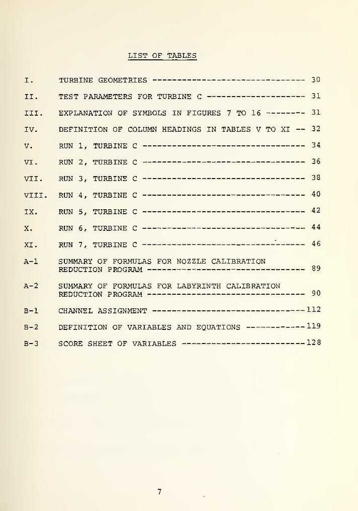
LIST OF TABLES
I. TURBINE GEOMETRIES 30
II. TEST PARAMETERS FOR TURBINE C 31
III. EXPLANATION OF SYMBOLS IN FIGURES 7 TO 16 31
IV. DEFINITION OF COLUMN HEADINGS IN TABLES V TO XI — 32
V. RUN 1, TURBINE C 34
VI. RUN 2, TURBINE C 36
VII. RUN 3, TURBINE C 38
VIII. RUN 4, TURBINE C 40
IX. RUN 5, TURBINE C 42
X. RUN 6, TURBINE C 44
XI. RUN 7 , TURBINE C ' 46
A-l SUMMARY OF FORMULAS FOR NOZZLE CALIBRATIONREDUCTION PROGRAM 89
A- 2 SUMMARY OF FORMULAS FOR LABYRINTH CALIBRATIONREDUCTION PROGRAM 90
B-l CHANNEL ASSIGNMENT 112
B-2 DEFINITION OF VARIABLES AND EQUATIONS 119
B-3 SCORE SHEET OF VARIABLES 128

LIST OF FIGURES
1. Turbine Test Rig 47
2. Turbine Blading Arrangement 48
3. The Floating Stator Assembly 49
4. Turbine C 50
5. Pressure Tap Location for TTRConverging-Diverging Nozzles 51
6
.
Turbine Test Rig Geometry for TurbineConfiguration C 52
7. Ref. Rotor Torque vs. Ref. Speed 53
8. Efficiency vs. Ref. Speed 55
9. Efficiency vs. Isentropic Head Coefficient 57
10. Theoretical Degree of Reaction vs.Isentropic Head Coefficient 59
11. Effective Degree of Reaction vs.Isentropic Head Coefficient 61
12. Stator Loss vs. Isentropic Head Coefficient 63
13. Rotor Loss vs. Isentropic Head Coefficient 65
14. Flow Angles vs. Isentropic Head Coefficient 67
15. Flow Angle (Alpha 1) vs. Isentropic HeadCoefficient 68
16. Ref. Flow Rate vs. Isentropic Head Coefficient - 70
17. Calculated and Measured Interstage Pressures 72
18. Calculated Interstage Pressure as a Fractionof the Hub-to-tip Pressure Difference 73
19. Effect of Smoothing Interstage Pressureon Loss Coefficients 74
20. Effect of Assuming Constant Referred FlowRate on Loss Coefficients 76

A-l Test Rig Piping Installation 94
A-2 Flow Nozzle Geometry 95
A-3 Views of the Flow Nozzle 96
A-4a Piping Arrangement For Labyrinth LeakageCalibration Tests 97
A-4b Piping Arrangement For Flow NozzleCalibration Tests 98
A-5 Flow Nozzle Calibration Data ReductionFlow Chart 99
A-6 Flow Nozzle Calibration 100
A-7 ASME Discharge Coefficient 101
A-8 Plenum Labyrinth Seal Leak Rate 102
A-9 Plenum Labyrinth 103
A-10 Labyrinth Seal Kinetic Energy Factor 104
A-ll Labyrinth Calibration Data ReductionFlow Chart 105
B-l Data Reduction Schematic 131
B-2 Control Volume a 133
B-3 Control Volume b 133
B-4 Thermodynamic Process of Fluid in anAxial Turbine 134
B-5 Velocity Diagram 135

ACKNOWLEDGMENT
For the many hours of counseling and assisting me, I
want to thank Professor R. P. Shreeve who showed a genuine
interest and concern in my research. Without his analy-
tical brilliance and expertise my research would have been
impossible.
Secondly, without the technical assistance and advice
of Mr. J. E. Hammer the experimental part of my research
work would not have been feasible. His countless hours
spent in preparing and running the turbine test rig for
my experiments are greatly appreciated.
Lastly, I want to thank my wife, Peg, who spent many
hours in typing my original manuscript.
10
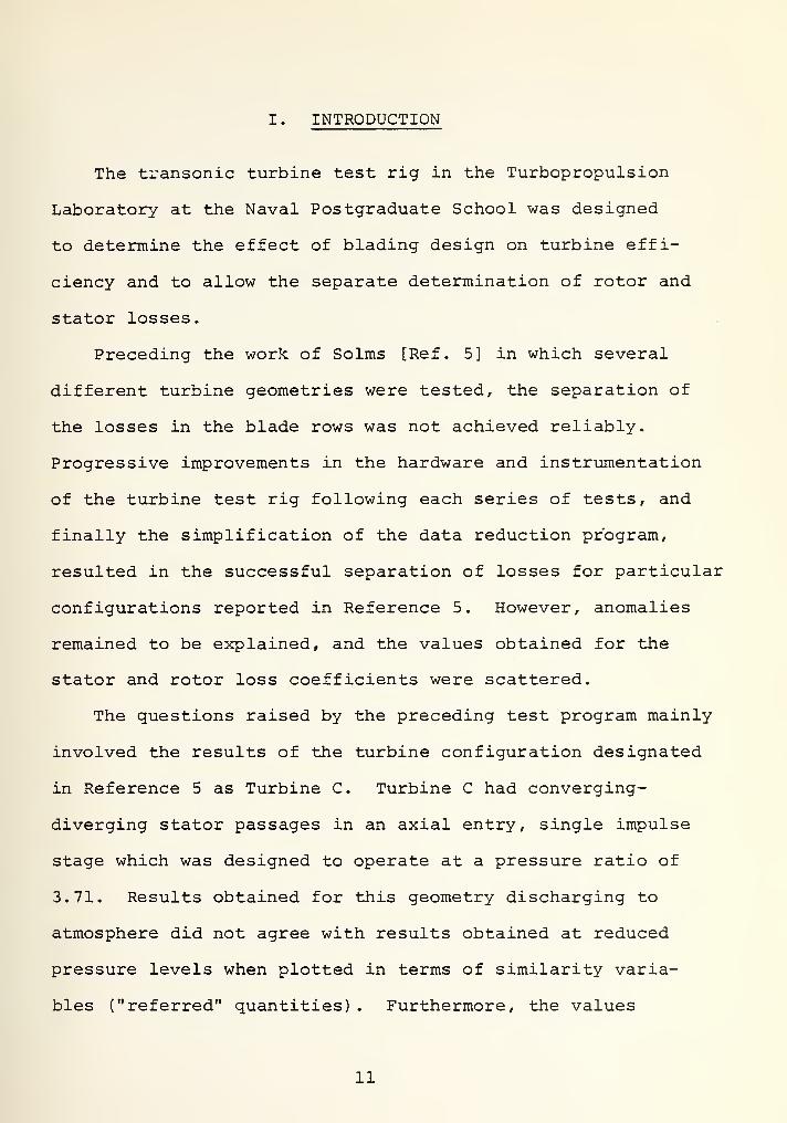
I. INTRODUCTION
The transonic turbine test rig in the Turbopropulsion
Laboratory at the Naval Postgraduate School was designed
to determine the effect of blading design on turbine effi-
ciency and to allow the separate determination of rotor and
stator losses.
Preceding the work of Solms [Ref . 5] in which several
different turbine geometries were tested, the separation of
the losses in the blade rows was not achieved reliably.
Progressive improvements in the hardware and instrumentation
of the turbine test rig following each series of tests, and
finally the simplification of the data reduction program,
resulted in the successful separation of losses for particular
configurations reported in Reference 5. However, anomalies
remained to be explained , and the values obtained for the
stator and rotor loss coefficients were scattered.
The questions raised by the preceding test program mainly
involved the results of the turbine configuration designated
in Reference 5 as Turbine C. Turbine C had converging-
diverging stator passages in an axial entry, single impulse
stage which was designed to operate at a pressure ratio of
3.71. Results obtained for this geometry discharging to
atmosphere did not agree with results obtained at reduced
pressure levels when plotted in terms of similarity varia-
bles ("referred" quantities) . Furthermore, the values
11

obtained for flow rate were of questionable accuracy since
the existing flow nozzle was too large. Also the correction
for a labyrinth leak rate became a more significant fraction
of the turbine flow rate.
The goal of the present work was to determine the blade
row and stage performances of Turbine C, while resolving the
anomalies reported in Reference 5. This would allow the use
of the test rig to investigate effects of geometrical changes
(stator-rotor separation and tip clearance for example) on
the losses. The first step was to design and construct a new
flow nozzle for the range of flow rates required by Turbine
C. The flow nozzle was carefully calibrated against three
different nozzles operating choked. The leakage rate for
the labyrinth seal was also measured and a semi-analytic
representation of the leakage rate as a function of pressure
ratio was obtained which should apply at different tempera-
tures. These developments are reported in Appendix A. The
existing data reduction program [Ref. 5] was revised to
access a Hewlett-Packard Model 9 867B Mass Memory unit. The
revised program is described fully in Appendix B.
In the results of the test program given here in Section
III, the effect of pressure level reported in Reference 5
was not observed. The scatter in the loss coefficient however
was not removed by the improvements in the accuracy of the
measurements. In the discussion in Section IV, a method
for smoothing the loss coefficient data is demonstrated
12

which will then allow a useful study of the effect of axial
and tip clearances to be carried out.
13

II. TURBINE TEST RIG INSTALLATION
A. DESCRIPTION
The test installation consists of three major components:
an Allis Chalmers twelve stage axial flow compressor, an
exhauster assembly, and the turbine test rig (TTR) itself.
The compressor is the source of driving air for the TTR
and for the exhauster assembly. Fig. A-l shows the piping
arrangement. Turbine air passes through the first settling
tank into an eight-inch pipe containing a flow nozzle, into
the second settling tank and into the turbine.
Fig. 1 shows the plenum, the floating stator assembly,
the rotor, and the dynamometer [Ref. 5], Pressure -ratios of
6:1 can be achieved when the system is hooded. The hood
was needed to achieve near design pressure ratios in the
tests reported here. Fig. 2 shows the turbine blading
arrangement of the stator and rotor. Ref. 8 contains detailed
description of the test rig hardware.
The floating stator assembly depicted in Fig. 3 permits
measurements of the stator torque while axial and rotational
movements are detected by calibrated force transducers that
are heat insensitive. These measurements allow the deter-
mination of the axial and tangential velocity components
at the stator exit [Appendix A, Ref. 5].
In this report one configuration designated Turbine C
was tested, the geometry of which is shown in Fig. 4; Table
14
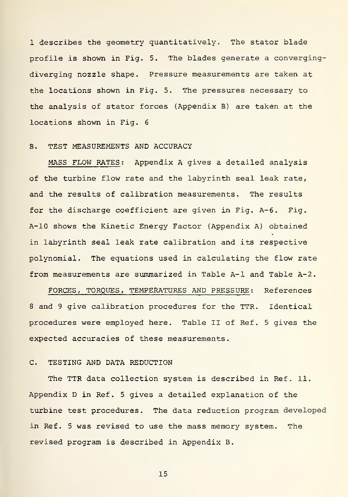
1 describes the geometry quantitatively. The stator blade
profile is shown in Fig. 5. The blades generate a converging-
diverging nozzle shape. Pressure measurements are taken at
the locations shown in Fig. 5. The pressures necessary to
the analysis of stator forces (Appendix B) are taken at the
locations shown in Fig. 6
B. TEST MEASUREMENTS AND ACCURACY
MASS FLOW RATES : Appendix A gives a detailed analysis
of the turbine flow rate and the labyrinth seal leak rate,
and the results of calibration measurements. The results
for the discharge coefficient are given in Fig. A-6. Fig.
A-10 shows the Kinetic Energy Factor (Appendix A) obtained
in labyrinth seal leak rate calibration and its respective
polynomial. The equations used in calculating the flow rate
from measurements are summarized in Table A-l and Table A-2.
FORCES, TORQUES, TEMPERATURES AND PRESSURE : References
8 and 9 give calibration procedures for the TTR. Identical
procedures were employed here. Table II of Ref. 5 gives the
expected accuracies of these measurements.
C. TESTING AND DATA REDUCTION
The TTR data collection system is described in Ref. 11.
Appendix D in Ref. 5 gives a detailed explanation of the
turbine test procedures. The data reduction program developed
in Ref. 5 was revised to use the mass memory system. The
revised program is described in Appendix B.
15

Seven tests were conducted of Turbine C at pressure
ratios from 1.75 to 3.25. The parameters and conditions
of the tests are summarized in Table II.
16

III. RESULTS
A. INTRODUCTION
The reduced data from seven tests of Turbine C are
listed in Table V to XI. Table IV gives a listing of the
symbols and meanings of the Table headings used in Table V
to XI. Plots of the reduced data are presented in Figures
7 to 16. Table III gives an explanation of symbols used in
these figures.
Tests 1 and 2 were conducted with the hood off. Tests
3, 4, 5, 6 and 7 were made with the hood installed. Tests
5 and 6 were repeats of tests 3 and 4 respectively. The
results are discussed in the following paragraphs. '
B. TORQUE
Fig. 7a and 7b give the results of the referred torque
versus referred speeds at a constant pressure ratio. A
nearly linear dependency exists for all seven runs with
consistency in performance for the 1.75 and 2.25 hooded and
unhooded pressure ratios.
The results from the unhooded tests (Fig. 7a) agree with
the results of the hooded tests (Fig. 7b) , at the same
pressure ratio, to within 1 percent.
C. EFFICIENCY (TOTAL-TO-STATIC)
Figures 8a and 8b give the results of the total-to-static
efficiency versus referred R.P.M. Figures 9a and 9b show
plots of efficiency versus isentropic head. The maximum
17

efficiency occurred at similar values of the isentropic
head for all pressure ratios. Ref. 17 relates efficiency
to isentropic head. The peak efficiency was achieved at an
isentropic head coefficient between 4.0 and 4.5 for both the
hooded and unhooded tests.
The efficiency is seen to increase as the pressure
ratio is increased, approaching 80 percent at the pressure
ratio of 3.25. The efficiency would be expected to increase
to the design pressure ratio of 3.71, at which the stator
nozzles should be just correctly expanded.
D. THEORETICAL DEGREE OF REACTION
Figures 10a and 10b give the results of theoretical
degree of reaction versus isentropic head coefficient at
different pressure ratios. Ref. 5 and Ref. 17 give the
equation for the theoretical degree of reaction. For all
runs the theoretical degree of reaction was negative at
lower speeds. For a negative value, P2/P. must be greater
than P./P . The values become positive only at high r.p.m.
in both the hooded and unhooded configurations, passing
through the design value of zero at a value of the isentropic
head coefficient corresponding to the maximum in efficiency.
Thus, negative values of the theoretical degree of reaction
occur at speeds lower than the design speed at a given
pressure ratio. Typically, there is seen to be also a loss
of three to five percent in efficiency from the maximum
value as the isentropic head coefficient is increased 100
percent above the design value.
18

Results from hooded and unhooded tests are seen to
agree with the exception of Run 3 in Figure 10b for which
the values are low. Lack of agreement for the data of this
test was found in all but the overall stage performance
measurements
.
E. EFFECTIVE DEGREE OF REACTION
Figures 11a and lib give the results for the effective
degree of reaction versus isentropic head coefficient. At
all pressure ratios, hooded and unhooded, the effective
degree of reaction was negative at lower speeds. Ref. 17
states that the effective degree of reaction is a means for
judging whether the flow is being accelerated or decelerated
in the rotating cascade. The negative degree of reaction
in Fig. 11a and lib show that the flow is decelerated at
lower r.p.m. and becomes accelerated as r.p.m. is increased
(Isentropic head is decreased) . In no case should the design
value of the effective degree of reaction be less than zero.
As stated above, operation at speeds less than design speed
results in a loss in stage efficiency, partially due to the
undesirable deceleration in the rotor.
The results for Run 4 (at a pressure ratio of 3.2 5) in
Figure lib reflect the marked improvement in efficiency at
pressure ratios approaching design.
F. STATOR LOSS COEFFICIENT
The results for the stator loss coefficient are shown
in Fig. 12a and Fig. 12b. While there is some scatter in
19

the data, the results from hooded and unhooded tests are
seen to be in reasonable agreement. There is a slight
increase in the stator loss as speed is increased at any
pressure ratio. The stator loss for the highest pressure
ratio (3.25) is significantly lower (13-17 percent) than for
the lower pressure ratios (18-25 percent). This reflects
the poor performance of a converging-diverging nozzle at
pressure ratios less than design.
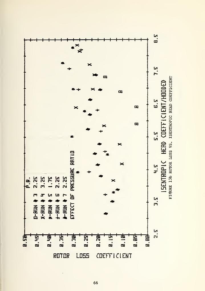
G. ROTOR LOSS COEFFICIENT
The results for rotor loss coefficient are shown in
Figure 13a and Figure 13b. For completeness, the results of
Run 3 have been included where the rotor loss coefficients
were evaluated to be positive. Negative loss coefficients
were obtained at higher speeds in Run 3, indicating an
error in at least one element of the primary data.
The rotor loss coefficient is the performance parameter
most sensitive to small errors (and possibly unsteadiness)
in the measurements. The sensitivity arises because it
involves most of the parameters (see Ref. 5) previously
calculated in the form of a ratio of small differences. In
view of this, if the results of Run 3 in Fig. 13b are excluded
from consideration, the rotor loss coefficient for the tests
are reasonably consistent. The results for hooded and
unhooded tests agree to within 20 percent at corresponding
pressure ratios. There is also a definite decrease in the
rotor loss coefficient as pressure ratio is increased toward
20

the design value, and a consistent decrease as the speed
is increased at a fixed pressure ratio. The simultaneous
reduction observed in the rotor and stator loss coefficients
at higher pressure ratios is consistent with the increase
measured in the stage efficiency (Fig. 8 and Fig. 9)
.
H. FLOW ANGLES
An example of the variation in the flow angles at the
stator and rotor exits as a function of the isentropic
head coefficient is shown in Fig. 14. As was found in all
cases tested in Ref. 5, the variations in stator exit flow
angle and rotor exit relative flow angle are very small.
Also, the total variation of the relative flow angle into
the rotor is only about 6 degrees for a 50 percent change
in r.p.m. The results in Fig. 14 are qualitatively repre-
sentative of the results for each of the seven tests. The
exact variations in the measured angles can be seen in
Tables V to XI
.
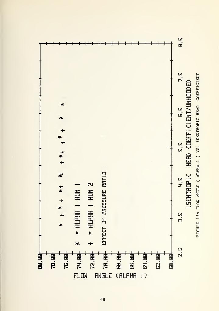
The stator exit flow angle is shown in Fig. 15a and
Fig. 15b as a function of isentropic head coefficient for
the seven tests. It can be seen that the measurements are
in the range of 75 to 77 degrees, with the lower value
occurring at the highest pressure ratio (3.25). It can be
seen in Fig. 5 that the suction surface of the stator blade
is designed to exit at 75 degrees, and the pressure surface
at a smaller angle. Thus the measured stator exit angle
appears to be slightly larger than would be expected; however,
21

the measured values when the nozzle passages are nearly
correctly expanded approach the geometrical angle.
The large values of stator exit flow angle at lower
pressure ratios, and the higher values of stator loss
coefficient are probably the results of the presence of flow
separation. The effect of flow separation would be reflected
in two ways. Firstly, the flow angle of the separated flow
could depart significantly from the trailing-edge angle.
Secondly, the existence of a region of separated flow could
seriously affect the averaging process which is implicit
in the data reduction.
I. FLOW RATE
The referred flow rate is shown as a function of the
isentropic head coefficient for the seven tests in Fig.
16a and Fig. 16b. The referred flow rate was constant at
1.02 lbs/sec to within the accuracy of the measurements
for all speeds and all pressure ratios when operating
hooded (Fig. 16b). During unhooded operation (Fig. 16a),
the results gave a constant value of 1.01 lbs/sec.
22

IV. DISCUSSION
A. RESOLUTION OF PREVIOUS ANOMALIES
In the results presented above, the difference in the
turbine performance operating hooded compared with unhooded,
is seen to be small. This is in contrast to the results pre-
sented in Reference 5. Three factors contributed to the
resolution of this anomaly; the accurate measurement of the
turbine flow rate, installation of temperature insensitive
load cells within the hood to measure stator loads, and
corrections that were made to the data reduction program.
There remains to be explained a difference of 1% in the
flow rate between hooded and unhooded operation. More data
are needed from unhooded tests to confirm that this differ-
ence is repeatable. Because of the sensitivity of the perfor-
mance parameters to the flow rate, the residual disagreement
between hooded and unhooded results might be resolved if
the difference in flow rates were explained.
B. FLOW RATE
The use of a choked nozzle to calibrate a large flow
nozzle was successful (Appendix A) . With the blockage
factor correction applied, the results for different sizes
of the choked nozzle agreed in the range for which the flow
rates overlapped.
The labyrinth leak rate calibration measurements were
well represented by the analysis given in Reference 7. The
23
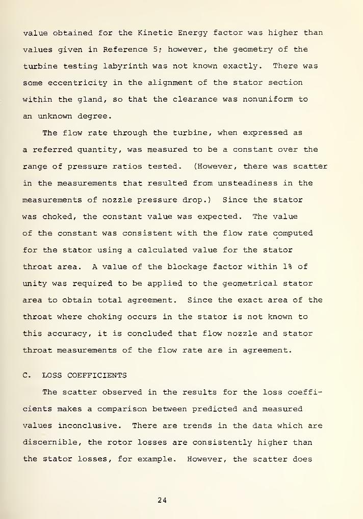
value obtained for the Kinetic Energy factor was higher than
values given in Reference 5; however, the geometry of the
turbine testing labyrinth was not known exactly. There was
some eccentricity in the alignment of the stator section
within the gland, so that the clearance was nonuniform to
an unknown degree
.
The flow rate through the turbine, when expressed as
a referred quantity, was measured to be a constant over the
range of pressure ratios tested. (However, there was scatter
in the measurements that resulted from unsteadiness in the
measurements of nozzle pressure drop.) Since the stator
was choked, the constant value was expected. The value
of the constant was consistent with the flow rate computed
for the stator using a calculated value for the stator
throat area. A value of the blockage factor within 1% of
unity was required to be applied to the geometrical stator
area to obtain total agreement. Since the exact area of the
throat where choking occurs in the stator is not known to
this accuracy, it is concluded that flow nozzle and stator
throat measurements of the flow rate are in agreement.
C. LOSS COEFFICIENTS
The scatter observed in the results for the loss coeffi-
cients makes a comparison between predicted and measured
values inconclusive. There are trends in the data which are
discernible, the rotor losses are consistently higher than
the stator losses, for example. However, the scatter does
24

not allow the effect of parameter changes on the separate
loss coefficients to be determined. The scatter is the
result of the extreme sensitivity of the loss coefficient to
the separate measurements on which they depend. For
example, the stator loss coefficient (z; ) is given by
s. = 1 ~ET (1)
where X, is the non-dimensional velocity and p, is the
calculated pressure ratio (P-./P. ) at station 1. Differ-
entiation of Eq. (1) gives, if X-, is constant,
IIId^S ^S Y-l P
lY dP
l2. = -r( E.) (lZ±.)
(i ± (7)
C sU
C sM
YM Y-D 3 PX
U)
1 - P. y
Taking the sonic condition of P, = 0.532, with y = 1 . 4 and
r = 0.2, the quantity in brackets has the value 5.78. Thus
a 1% error in calculating P, produces -6% error in the stator
loss coefficient. Since P, is derived (as is X,) from
measurements scanned over a period of more than a minute,
with some variation in operating point (as well as an
observable fluctuation in the flow nozzle pressure drop)
occurring during the data scan, the scatter in the loss
coefficient data is understandable.
25

Before the loss coefficient can be used as a measure
of performance, a method of smoothing the data while
retaining accuracy is needed. Two attempts were made
here. First, an attempt was made to smooth the calculated
values of the interstage pressure (p, ) , by comparing p,
to the pressures measured at the hub and tip. Figure 17
shows the variation p, and the measured pressure with
isentropic head coefficient for one particular test.
Clearly, the calculated average pressure at station 1 must
be smoothly behaved if the hub and the tip pressures are
smoothly behaved. An attempt to derive a smoothing function
for the interstage pressure is shown in Fig. 18, where the
data from several tests at the same pressure ratio are
plotted in a dimensionless form. The figure clearly shows
the degree of scatter in the values of P, . On the basis of
these data above, however, the use of a single polynomial
for the quantity (P,-P,1_)/(P J_ -P. ,) as a function of^ J 1 hub tip hub
isentropic head coefficient cannot be justified. When a
polynomial was derived from the data of a single test, and
the loss coefficients for the stator and rotor were recomputed,
the results shown in Fig. (19a) and (19b) were obtained.
The second attempt to smooth the loss coefficient
data involved effectively the elimination of scatter in the
input data from which the interstage pressure and velocity
were calculated. The referred flow rate was determined to
be constant when the stator was choked. By setting the
referred flow rate equal to the constant value (1.02 or 1.01,
26

hooded and unhooded, respectively) and continuing the data
reduction as before, the results shown in Fig. 2 0a and 20b
for the loss coefficient were obtained. A considerable
reduction in scatter is evident, with the major benefit in
the rotor loss coefficient. Further data must be examined
to fully appraise the benefit of this smoothing technique.
A third technique, so far not attempted, is to calcu-
late P, in the data reduction before calculating the axial
velocity component at station 1. The values of P, could
be smoothed using a polynomial curve fit and the smoothed
values of P, used to calculate the velocity. An application
of all three techniques should produce loss coefficient
distributions which are smooth and yet accurate.
27

V. CONCLUSIONS AND RECOMMENDATIONS
The following conclusions are made for turbine configura-
tion C.
1. The loss coefficients are extremely sensitive to
input data, especially the rotor loss coefficient. Repeata-
bility in calculating the loss coefficient directly from
measurements was poor.
2. Methods were demonstrated to smooth the loss coef-
ficient data without sacrificing, and possibly improving,
the accuracy.
3. For all pressure ratios there was a velocity
deceleration through the rotor and a pressure rise 'across
the rotor at lower r.p.m., indicating perhaps a shock wave
at or in the rotor.
The following recommendations are made:
1. Apply the three data smoothing techniques described
above to all data from Turbine C in sequence: input constant
referred flow rate, calculate interstage pressure and smooth
using measured hub and tip pressures, then calculate
interstage velocity.
2. Determine a more accurate input for K, , the ratio
of the momentum average velocity to the mass-average velocity
and examine the effect on the calculated stator exit flow
angle.
28

3. Program the quadratic curves for the theoretical
loss coefficient in references 16 and 18 in order to reduce
the input error.
Finally, it is concluded that following the recommenda-
tions listed here, the effect of parameter variations on
the blade row losses could be examined satisfactorily using
the turbine test rig.
29

TABLE I
TURBINE GEOMETRY
TURBINE STATOR ROTOR
C 1 1
DESCRIPTION A* 2(in?
NUMBEROFBLADES
\ix) (in.)
STATOR 1
CONVERGINGDIVERGINGNOZZLES
2.9058 31 4.184 0.5775
ROTOR 1 CIRCULARARC
7.119 60
Rm1
=4.193
Rm2
=4.2 5
h 1=0.732
h2=0.8475
30

wS3HPQ04
< enft w zH hi HH e_5 ^ O
Oi—
i
ooI—
I
oo
or-
1
oo
oI—
I
oo
o.—I
oo
o1—
I
oo
oI—
I
o©
J M /-» O O<!<![/] CM CMHW2 CM CM
< o ^ o o
oCMCM
oCMCM
oCMCM
oCMCM
oCMCM
wptf
S CMtn O ft
63 13 °ft < -uft ft ft
<|-
CM
CO
UCO
c
T3OO
4J
CO
Uo3
fl
OO
<L>
Ucu
5
m
CO
C3ft
CMmCM
m mCM
mCM
CU
C•r-l
.DU3
<4-l
O
>,UUcu
eocu
Ml
CO
cu
>•H
CO
H
CM CM co CM CM
>»CJ
acu
•HCM o
ft4-1
o 14-4
4J wft
v_^
^>II
o.—
1
O •H•H 4-1
o 4J CO
H CO 4-1
ft C/2
r-- 1
CU oc/) o h uW s 3 i
ft M CO i—
i
3 g CO CO
O 5 cu 4-1
HH H J-l oft s ft H
enl-J
OPQ
Cn
fto
OHH<
t-4
ftXm
oPQ
en
ft
ft
en
H
ft" CM CO m v£>
HO
ft
31
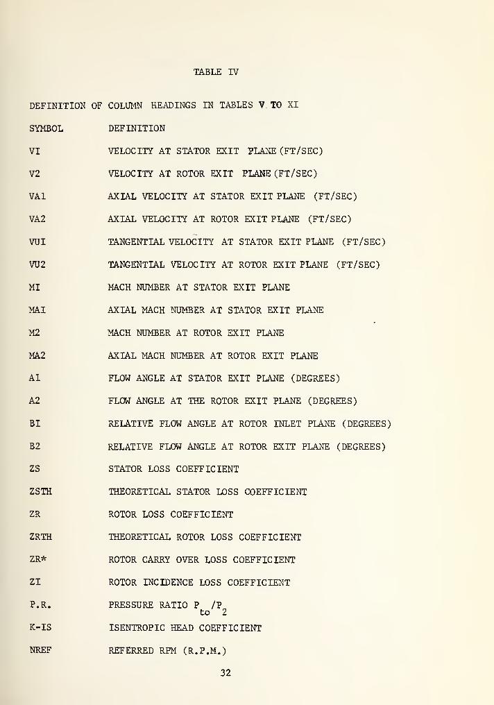
TABLE IV
DEFINITION OF COLUMN HEADINGS IN TABLES V TO XI
SYMBOL DEFINITION
VI VELOCITY AT STATOR EXIT PLANE (FT/SEC)
V2 VELOCITY AT ROTOR EXIT PLANE (FT/SEC)
VA1 AXIAL VELOCITY AT STATOR EXIT PLANE (FT/SEC)
VA2 AXIAL VELOCITY AT ROTOR EXIT PLANE (FT/SEC)
VUI TANGENTIAL VELOCITY AT STATOR EXIT PLANE (FT/SEC)
VU2 TANGENTIAL VELOCITY AT ROTOR EXIT PLANE (FT/SEC)
MI MACH NUMBER AT STATOR EXIT PLANE
MAI AXIAL MACH NUMBER AT STATOR EXIT PLANE
M2 MACH NUMBER AT ROTOR EXIT PLANE
MA2 AXIAL MACH NUMBER AT ROTOR EXIT PLANE
Al FLOW ANGLE AT STATOR EXIT PLANE (DEGREES)
A2 FLOW ANGLE AT THE ROTOR EXIT PLANE (DEGREES)
BI RELATIVE FLOW ANGLE AT ROTOR INLET PLANE (DEGREES)
B2 RELATIVE FLOW ANGLE AT ROTOR EXIT PLANE (DEGREES)
ZS STATOR LOSS COEFFICIENT
ZSTH THEORETICAL STATOR LOSS COEFFICIENT
ZR ROTOR LOSS COEFFICIENT
ZRTH THEORETICAL ROTOR LOSS COEFFICIENT
ZR* ROTOR CARRY OVER LOSS COEFFICIENT
ZI ROTOR INCIDENCE LOSS COEFFICIENT
P.R. PRESSURE RATIO P /Pto 2
K-IS ISENTROPIC HEAD COEFFICIENT
NREF REFERRED RPM (R.P.M.)
32

WREF
ETA
HPREF
RTH
REFF
PI
P2
P3
P4
P5
P6
P7
P8
P9
KBLOCK
STPR
RPM
REFERRED FLOW RATE ( LBM/SEC )
TOTAL TO STATIC EFFICIENCY
REFERRED HORSEPOWER ( H.P. )
THEORETICAL DEGREE OF REACTION
EFFECTIVE DEGREE OF REACTION
PRESSURE RATIOS CORRESPONDING TO TAP LOCATIONS
IN FIGURE 5. PRESSURES ARE REFERRED TO STATOR
INLET TOTAL PRESSURE
STATOR BOCKKAGE FACTOR
PRESSURE RATIO ACROSS THE STATOR P /P,to 1
ROTOR SPEED ( R.P.M. )
33

'AB L E
•-i V j. 'i j-
9 2 1 = 7
'-< !•-' 1 _'.'
9 3 9
«
E
4 n fi . ?
159
ELOCITY TRIANGLE: n i
'i
": 4
2 O >'. 4
i
V i-1 ::.
140. 2
i 3 7 » 9
£ o h- 3 ;:
284, G
! I ! !
V u
O -J :i J
y y
3 e 9
r i =
:
ir-n. Pi U i i b c I-
M2
J , 1 d i-i
nNLbt
b
FI.. 1 ?6 e, 1 1 ;-i
1 C T U.
- ' T < t
Fi . 1 Fi7 1
M .. -
.i~ i n:
!-i
,:, i- i
i-:.' » c 4 p' L
i-1
4
— L
i , Fi F - Fi
!r:
—i-J
— Fi
-Fir
34

RUN i.
F'T.n r.r . K .
1 . ?f
TRBLE JRB1NL
i . ?
-t » c ~
K : „ ;
i . 4 b b''
'. i r« r- r-i"1 r, h r L'l R E F ETfl -...j
f.
'"j- P ,';
., - ,-. .--. —i —
.
1.91 tij
r;-__
';_,
1 ;-"; i 1-,
,j-" j \.' 1 -"* ;' j
-'
|
:
* '"•u * -
1 y .:' £ y . 1 1.81 3 L:> 1. 6 o '!•
i 8 . 3 1... jj 8
"
jkj ."*( kT sf a i' 1 ; 8 6 3 i. j
.-. -1 18. 47 ,... ija
j| i
i 1359,
8
1 :. O^'t 8 . 6 9 7 1 . c 5 ,." .. . ~.!
'!. :
, _ .. „ _.: •- - i- „, • -
!! ! M !~! , H • . K 1 1- ."'
i £ £ 8S , 1 j a 8 i * 7 8 . 7 9 5 1 3 , 8 4 i"i p ;
s ';•. cr,
.-
•
1 . 885 8 .7' 8 7 8
;-; -
• •+ "i Kf •"*f~; i ">
i"-
j. i~'
1
1
j Q ,'-' C: ,~j
fl
"
HOZZL.£ P R E S 3 i' F E RRT i:
P3 P4 P 5 P b P |
.-, q <
w-': i.j. u.- v'J
8
8,
8 . :-! :-
t> i i. iZi U
.
/! .;!.!...
8 . 7 1
2
kl 448i.
:
. r' I b 8
,
„'i •.!(,':
i; .bi ..'bi/ q T P
tin 9 9 ? ^ i . 8 3
{.-jT
-i:
-H id 3 1 a C ^.
8 , 9 S 4 j.
i
a O ..
8, 937 _:
; I 7 3
y * :? 4
•J 4 J 9 9
u « b ig LJ
:•'! - n 8 :•
.-,-
1
;»"
-I'-,
"i
i U 5 U ti . -.1
11 98b .8
i 4888 , 8i ~S^H L~i
r ::•
9 , 5 8 3
y . - 1 b .•
8 ^ b 3 I
1 . h l'i
35

! p ! n r- tILL !
!'
D 1
J 9 3 r 9
1094.
4
1091.01088.21050.
5
1071 .
g
i r
ihiiU
i b ;', 4-
1 6 7 - 6 1 D I n 3
I 938 , 31 006 9
I."'!
i
'
mhl>M H N2
1 J.
!!!!._ !.J U •.
;
1 i.J .'
] 0191.010
1 4 b - i-1 . :•:.. I
0. 193*
. ' 9 F i
= 207
0, 10710a 1071
8 , 1 7
1
i" - iTi *?1 L7h -•; 1 O "'
H. ::
! h4
j . L O
36

1
"'
T R t \_ E. V I 1" JRE-INE
\ r\ r- —! -
!
h ! L !~ ETf1 . 9 U ::
:
• *
i y --> .." I , 9 1 4 I'J ,
:'._
cr .,7
1 . i
... ..., -
'l! a 71
I . 6 8 U i
:' H lj . 'H1
Buj lj c
» :'' .'.
516. 5 1 . :
::
'"' ""'
'
r~ "7 d 1,00
;
kl ,.;''
' f :" . '+] , U
'
"!. ; u i' ...
. b u b
,-.:;! i
:
- 1.
, :
•fi. fld
T O
y :, y i•• y ,
•!•
2', 00 -0 .
I~J .-i -
KJ- • *+i'
NIL: 1 ]
r, :
_ ,,. r, .j , , ..
i"' ~J F';-•
8
.
'+ 3 5 :*r -~i
'
g 4 :
'' Q*>
:: t ! .!•
',
i „ 4 r! H
J .. -i- k ! .:.
J . t d i
;-1 . H 4
M
a c
,-, cr.
r ?
.:.* J"_ \.:
-L-1
B
IT I .
..' i. .
M ••' '-'. A
7 , a
C -: ;":
».;;' y rj
d r * "J.! y a w J."' V ;
-; k ' by b y j
LH.
cr r
-->.-j 1 i
",
910, n •_i J. !' !^i a
. ! 'j -
37

p I. V 1
I 133.7
1 !S 4
1! i = o
J —I@.
.-.
i. i'-.'
1 f, Q . i"i
•-'i I
i U 1 i V "i" R I::
i II G [ ... E
V R
1
V hi 2 VU1. : S. > y 163. c-
i 183=
T
•"' "j Q 1 j£j ;-. 4 1
I8 . ]
- ' —' . •
•_- 3 - 1 ." : ' t 1083.1:f.
:
-: q 1 6 8 a 3 1073.
5
.': _" ;_.. a : ._' 1 C ."." a 1043,
i
. ;— —
,
.< .•• —
P
( •* •"• ~1 **«
'
\J :"* O L ~ :
i ~ T .!. fc.1 J b = £
56. 3 1 6 7 a 1021 ,
t
j .—, —
i
.: .— "
1
^ n , "i j.
:
-f rj = i .1 b b ! i y y • .
!
M 1
r j H i• " NI i-m
•IR 1
"i ] 4
i 4 4
A i .
u .?by
J 4
9 .14'
b = i j I-,
3 , 1371~i -I ,7- ~ 1
1 R7 1
i Q. 7 1
iK
~i . 976
:-' O O ll b .-
7 k 7' '-~
' V • i- 7 T
0.5535 -. 1:
'
:i 4 :
-
J
1 . 0E-:7-j -—' ;™ ;
"'
3 . 1 4 2 3 3. 4E-0cn i*r*i
. 3 8 6 5 5. 4E -0
i"-j--
fj ..:: ^ ;"i f-i
";
" "? "> : c ... Ci
M . 44 •
0. 03648, 1361
fa :.; 1 c H
.
38

TABLE
1 -i JCiiTh
i vi.•"' i~: i ;-;
1 » @ 1 9
1,81 8i . 9 1 5I .. 1 f,
;.: y pj
8 , P 8 4
8 ,?' 1 4
8 » ,1 P
n :• ': 1
, 1!.'
:
! f
H L ^ F E i
t6 Si!
Jh
•1A
i" -1 .-!'.' j -f T .
ki . 44 K> a O
8
.
:i
.
• i .;•;;-.;;
. i-
p r ;! I H
H Q "X 1
L. ...;
-i4 7:-
? r l -r
3 , !
'd 4 ] b
'_ a ..." T .'..
9 . 3 ^:
' S
Sj > T j. C
3 . 4 :"-;i"
39

I" I
'•.' i
Q,i
1 3CTy a y
1•~j
5 £i B U
I•~i
ill
ET "7
":-: y
TURB [NE
1
h i~
:-"1 , o
5"?
4 1 3 I F" . 6
i 3 I y . 3i
•":i v ~
i2
'•-: i
'inL-n :iu
; t
pKi :
fc'
34
!•! .
k!
.
,ii i
1 i L
i 17 'O
A '.'
r i , °^-0 C6 \ H
8 . 1243 :"j i" '!i ~5 H
K) O X r_' i' i.
8 , 1 3 3 9 9, 1971@ . 141
8
:~i 1 L~- / 1
!~ "! ' ! ~ ~ -j Jl~4
™? 1U a W : I
8 a 13 7 9 9 - 1 9 7
1
;.". j= fs f. 1 fi? 1
p 1 £j.i^i
9, 19719. 1371
m
v,.-\
9,
fcj =. i t" 4 Ofi 1
' 5 Q 1
j. i R d .1 1
•i .-' '--i -A -:
y: , c -+ t! :.-
9 2 3 3 ?
3 = 1 8 6 7
9 . 1 I- :
' C
3 , 3 9 9 9
9= 9977
-:f~ -j.-r
-• rv.""
5E-0:
40

KU-i 4 T:;
5
;
v= j_ cE '/III n. i'- r i h -
r « r.
3. 1
:~i - .*i >2- i £ ~i ,;
t 3,r - i:.1
.1 H
8 . 1 4 1 € £":„ :
:^|„ d 2 L
-" —• -"Ij .
-?'!"'.I-,
1 ,';:,; , ,.*
—| J .-,i
: ~>::-. i
"• '"' 1 1!
" "I'~ J. ...' .1 hJ rJ . '-: 3
6 = 9 7 .-. ..',' '-.i --
|.1 •j 6
'
: i 9
h -4 ! 1 4 i 3 9 = R @ 1:
';
r- : - sr1 4 3 8 .
4 ^i~i
>1
--' ,• O -J -- .L = -j i. i
b = £ b 15644. ~'j
; 3 2.-1 ^r o
l"i! !" ; h
< 1 -> , -j .- j .-. 4j 1
"i'
"
: :'"it I i • 1 i' _' i ".' 5 .'. 1;..! £ l:J
iH . 74
i r i\ fc. i~
i Q -0I
•
'
•,l.i - 6 !'"
'
a •„' "T - 9 I
;-iy , 4
40, I
4 ':.' a J
'1 , • I-
'
. H •. ,' -.' ..
'
I .. I"'
k1 .
kl . 4 4 :•'
,
ki .44 i
,-:__
;..: ;_; ij
i- 1 , h'j :•
; ;i .n.
:"'> '. it
i ;~: ~.'i is crrr-i-Ti1 - t ;*_' V a -' '_'
.
'
- .*! ~\ "i E" 1 |~j
_~ i£i - i-J 9 . 5 1
3 ; . 5 ? -:;
"' "' 4
-:. !
:
-i
41

' |M TRBL!
1 4 U * .
:.'
'-i i. f j-. J.
8 5 3 . 9
1 1-.
14':). f
\ 4 ':'] « :
/
I 4 . B J
• ; - ! - i .
1— ;.— '- • - J. I
::. ibi o
2 y 7 . a
r:"
fl j..
1
1-j^
jr
V fl £
i 4 1
.
9i i i
"'. .—
,
1.'".
i 4 y :, sC.
1 4 U ,-'-
I •.:''r.:
1
.. •J
i .-• -i•~:
1 "T I ;i kl
1 3 7
.
Q> >
i 4
J. t .!. „u.
-: d -I
-it -l!-;
78.4
•J O v. 1 7
i!n!
MR 1
eV'ii?9 , 19 3
L; 1
1 ";d
MM
-_' a i
HIRNLGE:'-;
|_, ;..
i
-' t . -'J d . y j~.
J—,'
"
O i''.': i r . y :
" £"i
:;
i '~ E l_ £6. 4 !li: O u •..."
r r . y O fel n D b '
. i
76.9 4 4 . 5 5 7, i
a „ t!
y = i." yo u
h cL ft -I £ r% *
7
1
y 3344 ( ;:. t ,i .
37 @ '.: J £ i
•
"7 i
y .
": .^ C -~t :~ -i ~ •
::2 v! .;' 4 y '"
i i Ci~ 1 |7h '
.
:
) t
". 7j y » l
J . 1671 k! .
'
!
3 1 7 1 fl 1
, :
|
.;...,,,-
3. =:+y :' ;• U. Lb-l-
5.4014 : 3 _. ;>':.
i. 3 6 1-'' S.ll 9
.. 6E-
42

KL HELL T ! ; P R T !-.! P
r . K
.
1 = 75>IS
d 1
L+ = 'r1 ('
i t!.-; "••*!-,
N i "! c h pI i"1
i [•j
£ '|~, - .;. u.j.
1 „ 1 4
t' £' ' .'
, 1.j
i , 2 6 * g 7 7! f i !
'"' [";
t 6 J !
:'
1 . 2 S S a 6 S
, 'i-t :-: !
„
.„.,
|
... ^
1 p v 3 : ,-,
1"7
.1. I u
13.
--;•'! . kl _!
£1 a fc3
i , ft
. n _.; u r . .. i :
h' !
0. 4
p-3
kl .. .j . ~i
i1 = J ~r O
H . 5 1: y • H i
= y y t<
i.eei;
1 . 907n '7* I-
1 7 '
1 = 014-
0,4-
1 I O il hJ O
1. 313111 3 ! Q i •-'
1. 1 >' "-! O1. 7304i a
"7 1 ."• O
•yJ
1 ..: :_! . i H
« Q < 1 1 '.
|7; 6 5 <
:
:
0, 6 1 5
pC|
•^:
» 5 64 * J t'
. 5 1
p Q
43

RUN ! MDL.C
i L
-. i
-;.. h
1
!1
1; B I NE
.....
r...
lr
L I C " --
1 7 '!
M ':
vui1 8 9 9 u ]
lie?.
i
1891.41873,
9
1 851.6I iT-t.-i i .;•!
i 1J -r -r a '•..'
i L"i !"i R 1
-1. H ' >
' \\'\ RNLGE
n ,:::
;.-]~
.
7j i D 3
r
_i v!
I- I 4 _i
. , j r " • v
44

p p k''~
, i y
Z :, 66
TflBL
NREF£ ( c i - i
i 111.51 '-'
i 3 »c
.-! :% -1 —
T i" ; D ? ! : - i
'
S- a ;:
kik'GF
1 • ,:. 3
• 9 ;
: : '• '. :
1,823':
,;J d. S-
l , 0^0i = @
'
i . 2 i
. b :-!
6 , 7 8 '•;
6 . 7 Q P
, 786
i , i''jy
?2 ;
5
1-1 O IS
2 6 ..
h 1 i
'
0,1! ....
;
El.; -0
. 08 •- 8
a S 7 - Of :
; i':
i
r". ...
i "l':: s U •
.
! M
» 6 3 ~8..
:
- i/j
iT-j .4
p p p p q ;:. j i p ;.:.
r •.•:•
.-; ! .' J
L- ;. T .
,~
. ~T -1 -,
rJ - ! t'
'•_':. "t L J.
., 4 9 i'"'
,. 496"'
„ f,;' 7
y l i* r"i
9 9 1 6
0800 It- 2
1
~! 7 tr
-. -. j -7
ts u i
Q.Q :M y
:i>' y L i 6 9 *
l#.i
fcl Z' I''?
.
... i._j .i
. 09 i 4 4 il! rj •J.' . nj qq
~! u/1 28 4 .
i"-i—
' 'i~
3 i 8
i i 1 3 4 9 =M j~H 519 . 3 3 5
1 r. £ 1 4 3 d 9 = jj , 5 1 9 hj j -.Jr-r o
It 1. 15290. 8 , '—' j. ••
T-i w i' b""7 1
1 b b 6 .:""-i
i
CTi
i,j
., 4 3
45

XI
i,,-4 -j-
2Q I ..
'
,_;. i;
I
{} I b
1 , 8 1 8
!. . 094y 990
„ * 7 ":
L„ :' 'i 1
1HUH i!URblyj j
3. 146J :: .!.
ktO
'..'. i
'-! ..
~. I n cl :.
. i., L fj _._
ii
•+ >
: , L ..
'
;;!,
:..' 5 ' >
l( i ! '
:•
• :-' 1
'' y
_
|.J
'
i
*"
.: i 4 j.
.....
I I"
! I
'
fa ii c
40. i
•. i
•j1 D ,. i.
i. i i
j..j '..,
I . h
-• '~: y a 8£ 00 ''
'
' '
k ;;. i
i
i ' - |.-'i
1 b hJ „ 0000 i-.i! • "'
"
:; ! !
'; ' i
i ;
': bE -ki
•013 K_. ,. 3 i: 3 ]
.
, !000 i
ti-
.954 rj K!
i 2 3 4
!
P 000 i
i.-i! 4 ., . j iE- fa
.
' r
:
fa KJ B £ 'J >.'. 1 :»' k i
•
..'ii 507
* M ^ "? r_: 0000 ;. i 195 i i 0000 1.
1
:8 ••'i
!"•" 8,7: !
'
!-_! „ 8 9 i !
j !
.
'. 000 i'". 1
: 90 . :( '0
:i
9
~
:"a 3000 ! d t? il". i! , 00! i
„ :. 2,2E '
;;i
1 1 3 ?!~H
|i
. 1394 00I-J0 1i
,
'i
' !.
..': vp ...:',
5:-84 --.' n 8800 :
j. L b" 8 80 fa;i 045 :,
;
.1 £ O L 8000 ;.:i 42b 8 0098 .. : 849 : . 9 E (
!
i i y r' '- u 8 I! ' 8 0000 8 .. : 065 ,. 01: 9
_ _
.
.. _ ..... » .. .... . ... ., ... .. ... . . „
46

9cr
to
UJ»-
UJ
a:
3
o(6
<
a
UJ
c3©
47

^m

Li
IZH *m a:
tr2
Ui— ZJin GSz trUin_ h-inDin
49

FIGURE 4 TURBINE C
50

JH^nd -!V/dV#*"
CD<DCM
d
3nvij iviavh
mUJ
=3
tfl
7c
* "i
J~Si
~L K°~l R< vK U z
U h >a^ 2
51
(30 ;>
* 2(Y1 sa k \J
51

I .SB
PRESSURE TP.F5
0.1 IN. BETWEEN CENTERS
FIGURE 6 TURBINE TEST RIG GEOMETRY FORTURBINE CONFIGURATION C
52

—1—1
—
1—1
—
1—1
—
1 1 1—1—1—1—1—1—1-—
H
—
1
. , X
••
X
Xco
LJXXX
UNHDOO
XtoX
CO
*—ccCK
CO
CO
LJ01=3inin
• * LJQSU1X m OS
• r- rvj—4
CLCu • •— (M CO Ll.a
CO— Pi
J*» 4r Ld
zz Ll.
Z3 Z3 mcr cri ia x
• 1 1 1 1 1 I • i
& ' cs da cs ' da i ' i ' cb 1 ck 1 cs
csCOCOen
COCOCOLa
csca —
-
— OS
o:COCOCO
QWwCMCO
En
CO>
fOH«5OH
COCOCOCO
Mfa
dtrvi
cs coCO
COCD
csLa
cs3" IM
COCO
COCO
COLa
COCOCOCD
RET RDTDR TORQUE: (in-lbs)
53

\—I—
h
9 csi cs
csin
rf"
at-
*XX
QSLrll/lLrlt/lt/1•rvjnjr^rvirvj
o.
ma-uitnr^
QSCCOSOSQlI I I I I
Ld£>aa
os
Ldac=iininuasCL
Lua
idLuLulu
us'cs'us'us'us ' esiea'es
cscscsCD
CScs __CS 2EJ" Q-
Lu,UJOS
cscscs
cscscscs
Qwwfain
fa
zn>
tOHPi!
OH§
fa
fa
CSX csHirvi
cscs
CSCD
CSLD
CS csrvi cs
cs03
CSCS
ca cs• 03
csLG
RET RDTDR TDRQUE tn-uB)
54

(S
XXX
m
•t/iar
• •
q.— rvi
—P4
era:i iax
03Xen
03
oa
CD
CxUaax
ECOS
uOS
inin
a.
u.a
LULi_
ux
*en m
cs cs
La
cscscsm
cs•
cscscsLa
cs•
cscs __cs apa- ex.— q:
LL-
CS lj. . crcscscs
cs
cs4- cs
cscs
CO
00
oM
CSCS
CS cs1/1 CO
EFFICIENCY <T - 5>
55

H h H H
°J*
m
V
osrvirvir^rvjrj
cuVjpi— hjhj
t
z:
OSEg06OSPStill
*
UJ
aax
cas
uas
ininuasa.
u.a
UJu.u.ux
01 m *
cacacam
ca•
cacacaID
ca
S 2F3" CL.— OS
Ldas;
w
ca•
cacacaca
ca•
caca
ca caLrl CD
ca
awwP-l
CO
U->
00>
oWh-l
oMfafaw
J3oo
OMfa
EFFICIENCY (T- 5)
56

1/1
m
i/i*
t/i
in
LJ
n
Li
rvi
fa
aV*» ?
a*
Lw UU. ^LJ w
Lrt a w
Lrtv^ HI
^ >a: !HLJ O
!<5wHO
v^»M
t/1^— |X4
• a- UJ
X aOS
ctf»— o^gLJ gLn 3
E=4
ernaoicf or-S)
57

H H
asrvjnJt^rurvi
aTwrf—-nirvi
nxuitnr*
Z3Z1Z3Z13dsqsqsqids1111DXJfcHHIl
x of
xa?*
>c en
tfr *
as
of*
o
CEOS
a:
ininLdasa.
a
LdLuL.LU
* 14—'—Sr
Id
m
Lrt
r-
Ln En
LOH- EnWOLd O—
—
Q«s^« sLu
LJOMEn
l/i 1=3 O• V^ H
S5bl
a:En"
MLJ31 CO
>
v^«
t/l—
^
W• a.
3T a Mas En
EnH- Ed"9^
LJLn J3
CT»
in EDOn l-l
En
E3
IIIst/1
t/i
CM*
emciaitt a- 5)
58

8
ECOS
Lias
•uizrinasr-rjin
• • *ljD-—nJDS
EL
—hjl.a
33UaatL.
I L.*3XU
m
m
xCD
X
Xm
S
aa
xS3
C9
rvi
srvj
*
CD
LI•
1^-
HLI H- S
ID LJU4MOl-l
«N*» |X4
aaa Wu. ou.LJa
LI v^ PS
LI >
cc S3OLJ M
H
V^ 2LI —
^
b• a. O
3- o Wa: s*— a-^. ta
LJ olti •
BL1
•fl
PI O
csin
LI
PJ
s1
THEDH. DEE. Dr REHCTION
59

i*.
..
LJ
aa•a
isIDS
E•UlLrlLrtUILn
ccnjrvir-njuiua.
ri3~LltDU.
QSQSQSOSu.I I ML
cs
4** m
m
*—'—4"rvi
* *
•
m
iii
SI
sLD
B1
t/1
THEDR • DCB • DF REHCT I ON
a
fat/1 I—• ^^ fa
ID UJ oa o«^ qKM <j
u. 3u. SB
Ul eno >til v^ 53
• o1/1
l-l
H<£a yCC SLd31 fao
fa
V-^ yLI —
•
o• DL
J* aas
Bh-~^.
Ul ,nin o—
*
1-4
LI
m 9fa
60

•i—
h
H 1 1 H H h
aax
muas
a.
—rviu.aCO
33Unr.vr,u.
1 1LcxuCD
*eg
a ' *hj
i
i ' A ' A i
SI
LO
E5I
msi
Lrt
CD
Lrt
r-
wMMfa
Lrt *— o• ~^L a
LD UJ p
u. wu. >UJ Za o
Lrt v^«MH
• ULrt
ccS
UJ o31
3
Lrt
v^ oUlQ
• a.3" a •
U*as u<
h- W^^UlLn r-t—
•
i-«
Lrt S•
81-4
Lrt
HJ
EFFECTIVE DEE. DF REACTION
b
61

-\1 1 b H h H 1 1 1 H
h. 1/1
ci
03
03
Ld
a
ICCas
i
idOS
•t/it/it/U/iinosiMCMr-rMm
KLIMn—PIOCa.
pist/itou.a
03
zzzzv 03
irrrrrrrt!i t i id.
1 DXJK-hUJ 03
i ' AC9 PJ
cs1
* w
effective: dee. df REHCT I ON
*C31
1/1
m
lit H-
Ldun
n
i/»
pj
H
fafawo
U.en>
Ld 2Oa M
l/i ^ H
tn<s*
1cc fa
Ld o32 fa
1/1
<s*» faa• a. •^ CZ3 fa
faas w
faerf
§fa
62

I I I I I I 1 I I 1 1 I I I I I
m
d
a: r-Ld 3"
aaa:
a;
Ldo:Z3in
Q
ca
x
X
X
X
•a. — pa
im inLJ
a.
— pj L-a4*. *•
t—Z Z V^ZD 3 taJEELI I Lua x ui
GJ
X[23
X
Q3
A ' di ' A '
ili' A'ili ' A'A ' A'tli 1
Ld zr 3T n m PJ nj — —
•
Ss s EJ (S KJ S £3 IS EJ s
C3
L/1
m
Ld•
Ld• i—
LD 3UI
v^u
, fa
u.Lx. oLd u
Ld Qf V^ 1
Ld(£*
S3
CC CO>
Ldn: CO
COo
k^ oiLd —
•
O• a-
s3- act: CO
i—•^Ld CO
CNLn i-l
t
Lrl•
3
n
Ld
rvi
fa
ts
STflTDR LEE5 COEFFICIENT
63

I 1 I 1 I I I I I I I I I
XX
X
Ca.
LJ
aa
LJas
• i/i isi t/i lji i/i ink w n r- n w inLJ
a. w n - n n ka.
m 3- w to r* u.a
ff B ff E K kt I 1 I I Urna x « -h <* La
*»x
«n *
* x
» H
t/1 Xs s
3"rnnrvjrj — — cs
C9 CS C9 C9 ^9 C9 ^9 S
5THTDR LD55 COEFFICIENT
as
Li
LI
LI w• *— M
OHtil
UJ^^ W^ OuLu QU.
S3LJLI OLi*
V^ CO>
<£i CO
cc COoLul h4=
OH^ nLI •^ CO
• D-3" CZ3
as CM
•^LU 3LTI PoM
LI
m
LI
rvi
64

I I I 1 I I I I I I I I I I I I
aa
m
X
ECcr
Ldas
• in x inK h w in
a. — na osa.
- W Laz z ^3 3 Ucr cr u.
t Li.a x m
xm
m
CO
Lrtsrsrnnrunj — — ca• •••••••••CSC9C9C9C9CSC9C9C9C9
til
CD
Lrt
LD
wMCJHpt,
Woa
Lug
• tJ en
1/1 H
Ld >
Ln
3"
LI
n
Ld
s rwcs
^ ptf
LiJ _.
in §oH
RDTDR LD55 aEFTICIENT
65
I I I I I I I I I I I I 1 I I I I
*H- X «* m
CD
ta
.1
ccas
t/1
OS *• in t/i 1/1 1/1
Z3inB hj rvi r- HJ n in
• • • • • • UJ•a. n m ^^ ru r\j as
a.
n 3"* t/i ID r*- U.a•
2 2 -g 2 z C^3 *~n J3 ^3 ^3 UJOS OS OS OS as u.1 1 1 1 i Lu
. a X * -H 4k Ui
*
cb'di ' cg'il.'cs ' ik ' A ' tti'Ai '
ilii/io-a-pinnm — — csSSSSSSSSCSCS
t/1
ca
t/i
LU
caai/i
10
t/1
LU
1/1
n
t/i
cs
H55wMUHfafafaO
fa
V^ Sfa
HfaCO
CC. >"T" tQ-** CO
w IT 8
r— co
LU M
Mfa
RDTDR LD55 COEFFICIENT
66

\—I—I—I—I—I—I—I—I-
* X* X
* X
* X
* X
* X
* X
* X
H—I—I—I—I—
h
i/irvi
ias
a.
mCD
ca
ca
ca
m
m
uas
m— pj — pj aas
3: n: cc ccCLQ.HI- Lj juu acc cc ta to
II II ti ti §u.
co
03
s s caA ' A ' ^ '
eb' A ' Ai
1
m
bi
r-
Ldtf2a wC3 1-4
C3 M
LI ^*.
I*P*
• h- oU uLd 9V^»
1x4
s- -•
u. !—
1
u. PM
UJ at/l C3
• <^ §Lrt w
COc£s MCCLd •
CO= >
l/i
V^
• CL^ a3a:
t— p=i
"Z, v+Ld I-l
un§R
in M• P=4n
S IS03S
isi
oa S3 ca oa S oa oa S3 cam LD 3" IM P4 X LD1
CD1
F10W rngle degrees
67
I I 1 I I 1
— PJ
ccZ3q:
— —a: cc
—Jcc
ri ri
LJas
ininuasCL
LuO
uI*.
LuLi
(S A ' A'A'A'A ' lk'db'A ' Alcs cs B3
CD La ru CDID LD
XLD
rvi
LDCSLQ
FLDM ANGLE (RLPHH I)
Lrt
CD
til H• Z
r*- «C»—
LxJ o£* 1—
1
a PC4
C33:
oozLrl v. 5
LDt—
LJ HPu^ Otm
U-H2
u. WLJ c/3
MLd a
• «^CO>til
*2»nzLJ r-t
3:1
33P-.
<^ 3Lrl—
•
• CL.N—
3- wOS
LJ r-B
i_n bi-5
LrtCOmi—in
Lrl
68

1 I I I I
XCQ *
-Kn *
G3
4*G3
%
en
ca *
-K3- L/1 in i— CC
m Z z. z: zz. Ldm 33 33 =i ~~i CC
CE OS as as =3LTI
% — — — —LJ
>c CCCC cc cc cc a-
B3 n: ni DC T*.
CL, a. CL a. L-—
1
-j —I -j
encc
tl
cc CC
(1
cc
LJ
*.
LuLi.
Li
ISCS
csm
cs ' is'is'cs'cs ' cs ' cs'cs ' cs
Lrt
CD
LTI H• z
r* Edi-i
CJ
es HI
LJ fafa
C^J Wcn O
CJ
oz 3Lrt \
• H- paLEJ u
LJ H, eu
«^ oOSH
L*.Li. CO
LJ h-l
Lrt cn• ^ CO
Lrt
CC
>
LJ f—
1
= <33fa
^ si
Lrt— V—
*
• CL,3" fa
faOS uI— 5zLJ 3:
lh O
Lrt in• i-4
n
Lrt
CS CS cs CS CScs rwCS
LD or cs CDLD
LOLD
3-LD
ruLD
CSLD
FLOH RNGLE CRLPHR I)
fa
69

4—H 1 1 1 h H 1 h H 1 H
Ul
aax
m
to
xmx
Xm
CEas
Ulas3
• LQ a- inas r- rvi in
• • . Uia. ™ nj as
a.
— ro u.a*i-Z z v>3 =3 Uia as u.
i 1 u.a X Ul
Xm
xQX23
HJ — CS 01
Ul
ui
Ul
in
LJ
U.UJ
ui aui
ui —• a.
as;
ui
ui
wMUMfafawoo
w9CJMfa
HzwCOl-l
CO>
3fa
•
fa
at
uj-
!£1 §
fa
Lh rvai
REX. FLDH RHTC (lbs/sec)
70

H 1 H H 1 h H 1 1 1 H
-C
Ui
a
*
as
x
Ui05
)
ui ui ui
» • • •
a» n — rv
ui inrvi in
a*
3* U1 LD r» ti-cs-
3 Uias u.
-+t Ui
4ra 3 acr cc oi
i tax*
as
' ' ' UI 'H h * ' A ' ' '
UI
03
UI
I-
UI
UL
WMOMfaEdOO
9WPC
Ui a
51
1
U. gU. [i]
Ld en
ut a M
CO>
- tA^
ui — *» n
,
as £
Uiin
ui
-a
Oi-i
E=4
UI
01 m
REF* FLDH RHTET (lbs/sec)
71

I I 1 1 1 I 1 I I 1 I 1 I 1 1
>C -4-
>S -K
ca
** *
-*• *
m
m
m
LYtn*
rvK
•> <aas UA• 1—
B. cc
r» n-T-i
S^g1 I —1f^
n
-+* m
'Ja'ja'^'ja'^'t^'^'ja
Lrt
03
Lrt
CO
C/3
Lri 1— COw
• fe PSLQ Ld 0*
«*>^^
<JU. E-»
u. CO
Ld wa gLrt k** MLrt
<£>
1 a
cc COLd
ur
l/r
FT
aH
Ln g
aM
Lrt
LrtfU fAJ w S3 cn 03
ni — —
ca niss
LD
RDTDR PRESSURES
72

—1—I—H 1 1 h-H 1 H—
1
1
*X
*
? x * •
*
m03
-
-
'
*go x
DO
KT
*
OS
POO>
alt **
OXmm
m
|I
1—
O.
|
-
SBox*
* £
Sb! B3 i ca s cb I da I S ' flD
L/1
03
1/1
t/t I—to* S
Li.Li-LdCI
in v*»
uf
CCUJ
Ul
l/r»
in ut pi fM
in
P4
cao
to&4
gCO01MasPu
eu
KS
w
2O
Ito
03
8* -i
Cft. 5CU -">
Eh03
w
g
(3.MiP
g
St.
PRESSURE RRTIO
73

I I I I 1 I I I ) I I I I I 1
EX
A/-* LdA XUl 1—X oI— asa in^j zin =3\~r »-»
to La
41* *Z •z.
=2 =2as a:i iX
ISLrl
Htil 53
• wm M
OMfafafaOCJ
COCOo
Ld -J
•OSo<HCO
Ofa
t/i• h- CO
COLU ^^ Ed
Ld OSPUl'—^
^ faO<
u. Hu. CO
OSLd w
Ld ^• KS i—
i
Ld<0 o
Pien MUJ B
o3iosCO
<v*
Ld —
•
faO
• a~X a Ha: U
fat— fa
UJfafa
LTl <0
r-l
Ld•
• Mm fa
Ld
a* 3~ n m ro ni -— — b ea
5THTDR LD55 CDCFF 1 C I ENT
74

I I I I I 1 I I I I I I 1 I I I I
xn
X El
E3X
ca x
QSX
/-» L»J
Cx XUJ I-x ah- asa in
in Z3
to ld
z zcc asi ia x
xn
?C3
a 'di ' A'di ' A'ili'A'di ' A'ili' mt/ia-j-nirnpjrvi — — s s
i/i
CD
Lrt H• 85
r*»
oMfafaEdoc_>
COto
Lrt• H- s
LD Pi
UJ oHr o
V^» <*
u» O
Lrt
u.LJCI
w
• KJ COCOEdLrt
£h PS
nz P-i
Ul w
CO
v^ 03Ed
Lrt— H
• a- i—
i
J"
*—OM
LdLT1 8
2ca
Lrt•
fao
m HUEdfafaEd
-Q<J\
r-l
Lrt•
• Mrvi fa
eg ts is ts cs cs ca
RDTDR LD55 OEFFICENT
75

1 1 I 1 I I I 1 1 I 1 1 I 1 I I 1 I I
a...
>— UJa ^^;a h-
iaa;
* j§ s* trt trts m ru
a. rv rvt
IB U3
«M
; 15as. DCi I
* C3- X3
i
xox
ut r a- m n A ' A ' ttt ' A ' ftru m — — hi
lit
03
U1-4
E«*
111»
Ed
8r-
COCO
3
1w CO
•i
—
55UJ O
Ul EdH*-** 2MM»
U-U_ SUJ pE4
trt C3 a• V^
trt CS<*^» Edz fH
3UJ32
ks HCO
trt » SB» a. O
ar CJ
as. CD
H- 55i—
i
UJm COCO
™^*
irt o»
nr uEdEwfaEd
•OCM
trth4
ru ft.
5THTDR L055 COEFFICIENT
76

1 1 1 I 1 I 1 1 I 1 1 1 I 1 I I I 1 I
CD
UI
CD
CD X Ui
01 >c
AE3~r~ Q .
»— UJ ,a rea h-sz a !
ui ag»,Ui Uiw ru
1
ru wUj ui
as ccir a >;
xa
x ax
IDUJ
Ut
iA
XCD
UI
UI
UI
ax x
UJLTT
Ui
.' A ' A ' ili'A ' di'A'ili ' i'il.utSTD-nmrvirvj — — s
ui
H+fafaEdOUCOCO
01
8
25a
Br: 3
3:
3
QEd
fafa
E-»
ICO25OuC325
COCO<J
faoE-t
fafafafa
o
C3h+fa
RDTDR L055 COEFFICIENT
77

APPENDIX A
FLOW RATE DETERMINATION
A-l INTRODUCTION
A precise measurement of the flow rate is necessary
if the performance of an individual blade row is to be
determined accurately from measurements made with the turbine
test rig. Anomalies that occurred in the results from the
first tests of the present supersonic turbine (Turbine C
in Ref. 5) were possibly due to inaccuracies in the speci-
fied flow rates. Since the flow rate for Turbine C was
smaller than for the turbines previously tested in the rig,
small pressure differentials were measured with the existing
nozzle. Also, the higher pressure ratios at which Turbine
C was operated resulted in increased leakage through the
labyrinth seals , the geometry of which might have change
slightly on reassembly. Therefore, before new tests of
Turbine C were begun, a new flow nozzle was provided and
careful measurements were made of the labyrinth leak rate.
The flow nozzle design and calibration are described in
Section A-2. The labyrinth leak rate determination is given
in Section A- 3.
A-2 MEASUREMENTS OF THE TOTAL FLOW RATE
A-2.1 FLOW NOZZLE DESIGN
The flow nozzle is positioned in a pipe through which
air is supplied to the turbine (Fig. A-l) . The nozzle
78

generates a differential pressure to which the flow rate
is related.
For a one-dimensional steady flow, the mass flow rate,
W, is given by
W = p AV (A-l)
where p is the density, V is the velocity, and A is the
cross sectional area.
Using the perfect gas equation of state
pt
p = ss- (A-2)t
and Bernoulli equation
Pt
" P = \ P V2
(A-3)
Eq. (A-l) for low velocities becomes
(A-4)
The symbols P and T are pressure and temperature, respec-
tively, and the subscript t denotes stagnation conditions.
This equation, with explicit corrections for compressibility
and thermal expansion, is used to calculate the flow rate
through a flow nozzle from measurements of temperature and
79

pressures. Withe the addition of the correction factors and
with conversion factors added to account for the units of
measurements [Ref . 1] , Eq. (A- 4) becomes
0.16384 _ 2 _ v v /
PN
Ah... , . ,_ _,W = D A^ K^ Y /—5— (lbs/sec.) (A-5)
/2.036 N w w xJ
lt
where
DN = Diameter of nozzle (inches)
A., = Thermal expansion coefficient
Y. = Compressibility coefficient
PN = Pressure at the nozzle (psia)
Ah = Water differential (in. H20)
T. = Temperature (°R)
0.16384 = Conversion factor/2.036
and lastly, KN is the discharge coefficient.
The discharge coefficient accounts for the fact that the
flow is not one-dimensional, and that the pressures measured
are not P. and (P. - P) . Generally, the discharge coefficient
has a value above 0.95 for a standard ASME nozzle at high
Reynolds numbers. Establishing the relationship between
Reynolds number and the discharge coefficient is what con-
stitutes the calibration.
80

The flow rates expected in the supersonic turbines were
1.3 to 3.5 lbm/sec. A flow nozzle with a diameter of 3.25
inches was chosen (by applying Eq. (A-5) with unity for the
coefficients) to give sutiable water column measurements of
approximately 9.8 to 58.1 inches. The nozzle design followed
the criteria given in Ref. 1 for "Low Beta series" designs.
The geometry of the flow nozzle is shown in Fig. A-2 and
views are given in Fig. A-3. The locations of the pressure
taps are shown in Fig. A-2. Four throat taps are located
1.5 nozzle diameters from the nozzle face and are manifolded
together. The upstream pressure is measured using taps in
the upstream flange.
A-2. 2 FLOW NOZZLE CALIBRATION
The discharge coefficient is given in terms of measure-
ments, if the flow rate is determined by independent means.
One of the most accurate methods of determining the flow
rate of a gas is by choking the flow at a known area. This
is because the mass flux is nearly uniform where choking
occurs , and because the boundary layer can be kept thin in
a rapid smooth contraction from a relatively large pipe.
Hence, in order to determine the discharge coefficient of the
new flow nozzle as a function of Reynolds number, the
arrangement shown in Fig. A-4 was used.
A-2. 2.1 Method
Flow nozzle calibration runs were made at con-
trolled supply pressures from 15 psia to 45 psia. Three
81

different orifice plates with diameters of 1.6, 2.065, and
2.24 inches were mounted in turn to provide choked flows
over the desired range of Reynolds numbers. The differen-
tial pressure at the flow nozzle was varied in increments
of 2 to 4 inches of water. The range of flow rates over
which the orifice plates were choked at the supply pressure
was from 1.33 to 3.55 lbm/sec. The maximum pressure ratio
obtained was 2.92.
A-2.2.2 Analysis
The discharge coefficient was given by Eq. (A-5)
,
and the Reynolds number was determined by
48 W 3
i% = ^— (A-6)7T D li
P
where \i is the viscosity and 3 is the ratio of the diameter
of the nozzle to the diameter of the pipe. The flow rate,
which was the same for the nozzle as for the choked plate,
was determined by the following equation
where
rP A K
W„ = r t B(A-7)
N /RT7?
P. = pressure at choked nozzle (psia)
2A = area of choked nozzle (in )
82

K_ = blockage factor
R = gas constant (ft-lbf/lbm - °R)
T = Temperature at choked nozzle (°R)
The function r is a known function of the specific heats and
is given by
=p~<&W (A- 8)
The blockage factor K_ accounts for the boundary-
layer and for the axisymmetric surface; K„ is given by
[Ref. 3]
46*'B DK„ = 1 - =£- (A-9)
N
where the star on D„ signifies sonic conditions, and 6*N
is the boundary layer displacement thickness.
The boundary layer growth was estimated using
the method of Falkner and Garner given in Ref . 6 . The
displacement thickness, 6*, is given by
nHTT
i--5*__ ^n+1
(A-10)sl
Reln+1
83

where s, is the distance from the stagnation point to the
choking station. H is the form factor, and a and n are
empirical constants. ^ is a factor which depends on the
pressure gradient along the surface. Re, is the Reynolds
number based on conditions at the throat and s,
.
It is shown in Ref. 6 that the value of ty for
a similar contraction was 0.38. With ip = 0.38, and with
H = 1.4, a = 0.0076 and n = 6 for air, Eq. (A-10) becomes
m 0.09321746 I 0.1429 S
l{A 1L)
K6 ,
The Reynolds number is given by
W s.
Re, = 12 ^ — (A-12)1 A
x y x
where y, is the viscosity at the throat where the tempera-
ture is 5/6 times the stagnation temperature.
For each operating condition for each orifice
plate, Re, was calculated from Eq. (A-12) using W calculated
from Eq. (A-7) with K_ = 1.0. 6* was then calculated usinga
Eq. (A- 11) and K_ obtained from Eq. (A- 9) . W was recalcu-
lated from Eq. (A-7) . It was found that the blockage factor
could be taken to be constant with pressure for each choked
plate at the following values:
84

PLATE # THROAT DIAMETER Sl
(ins.
)
KB
1. 1.6 3.51 0.9928
2. 2.065 3.10 0.9935
3. 2.24 3.22 0.9901
The flow chart for the analysis of the calibra-
tion test results is given in Fig. A- 5 and the equations
used are summarized in Table A-l.
A-2.2.3 Results
The nozzle calibration extended over a range
5 5of Reynolds numbers from 0.081 x 10 to 0.213 x 10 . The
results are given in Fig. A-6, where the data for three
different orifices are shown for the range of pressures
for which the flow was choked. A second order polynomial
was found to represent the flow nozzle coefficient as a
function of the Reynolds number.
K., = 1.0272 - 0.1598 (—S) + 0.3805 (—5)2
(A-13)* 10* 106
where Re is given by Eq. (A-6) , was used to reduce data
from tests of the turbine test rig.
A-2.3 APPLICATION
The discharge coefficient is a function of Reynolds
number. However, in application the flow rate is to be
determined and therefore the Reynolds number is unknown.
The determination of the flow rate from measurements requires
the solution of three equations which have the general forms:
85

WN
= ax
KN (A-14)
Kg = KN
(ReN ) (A-15)
ReN
= a2WN (A_16)
These equations represent Eq. (A-5) , Eq. (A-13) , and Eq.
(A- 6) , respectively, where a, and a~ are known in terms of
the geometry and measurements for any operating point.
Clearly, by substituting for Re and K using Eq. (A-15)
,
and Eq. (A-16) in Eq. (A-14) , a single function for the
unknown W is obtained.
An iterative procedure is used to solve the three
equations for the unknown flow rate. The procedure is
given in Appendix B.
A- 3 MEASUREMENT OF THE LABYRINTH LEAK RATE
A- 3 . 1 Labyrinth Leak Rate Calibration Test
Since the leak rate of the plenum labyrinth cannot be
measured during turbine operations, the relationship of the
leakage flow rate to supply and hood pressures and supply
temperature was determined in a separate calibration test.
For this test, the main flow through the turbine was blocked
by a plate and the labyrinth was allowed to leak into the
hood as in normal operation. The flow was passed through a
two- inch pipe (Fig. A-4b & Fig. A-l) , containing an ASME
standard sharp-edged orifice. The usual supply pipe was
86

blocked. The flow was discharged through the labyrinth
seal into the hood in which the pressure was controlled
by the ejector.
In determining the leakage rate using the ASME orifice,
vena contracta taps were used. The differential pressure
was measured in inches of water on a manometer which had
0.1-inch graduations. The upstream pressures in the lab-
yrinth and in the nozzle were measured in inches of mercury
on U-tube manometers with atmospheric pressure as a refer-
ence. The supply pressure was varied from 14 to 83 psia,
while the differential pressure across the vena contracta
taps varied from 2.75 to 37.3 inches of water. The maximum
pressure ratio across the labyrinth was 5.6.
A- 3 . 2 Calculation of the Leakage Flow Rate
Since the flow orifice was in a standard installation
according to the criteria given in Ref. 1, Table 5 of Ref. 1
was used to obtain the discharge coefficient as a function
of Reynolds number. In order to program the data reduction,
the data of Table 5, for the appropriate values of Beta,
were first approximated in the range of Reynolds numbers
from 8,000 to 1,000,000 by a polynomial as shown in Fig.
A-7. The discharge coefficient at each operating point was
then given by
87

105
K__ = 0.603698259 + 0.004688755 (—-) (A-17)N ReN
5 5- 1.250025 x 10~ 3 (^—)
2+ 2.0320771882 x 10~ 4 {——) 3
ReN Re
N
5 5-5 10 4 -7 10 5- 1.56980769 x 10
D(£*—) + 4.5277098 x 10 (~~)ReN Re
N
The flow rate was calculated at each point using Eq.
(A-5) , using the expressions for the compressibility and
thermal expansion coefficients given in Table A-2, and the
discharge coefficient given by Eq. (A-17)
.
A- 3 . 3 Analysis of the Results
A- 3 . 3 . 1 Simple Method
A non-dimensional flow rate, or flow function,
for the flow through the labyrinth can be defined as
WT
/(R/g) TT
During the calibration tests, the stagnation
pressure (P ) was varied in steps for constant values of theLi
hood pressure (P,) . The stagnation temperature was approxi-
mately constant. The flow function was calculated for each
operating point using Eq. (A-18) and the values plotted as
a function of the pressure ratio (P./P.) . The results are
given in Fig. A- 8.
A second order polynomial was found to fit the
data to an accuracy of ± 4% as shown in Fig. A- 8:
88

$ = 0.2721 + 0.0365 (Pj/PL ) - 0.2357 (Pj/P
L )
2(A-19)
While Eq. (A-19) represents the calibration tests
results quite well, it is an empirical result for a limited
variation in test parameters. Operation at different
temperatures, for example, could give a different behavior.
A-3.3.2 Use of the Kinetic Energy Factor
It is shown in Ref. 7 that, under reasonable
assumptions, the flow through a labyrinth with many teeth
(N) can be represented by
$ = 3 Ke (A-20)
where
1-(P,/P_)2
* = / N-Ln(Ph/P
L )
(A~ 21)
and Ke is the "Kinetic Energy Factor". Here, the dependence
of the leak rate on the upstream and downstream pressures
(3) has been obtained analytically. The Kinetic Energy
Factor is a measure of how much kinetic energy is recovered
as stagnation pressure as the flow passes successive teeth.
It is expected to be a function of Reynolds number, and
hence would include the correct behavior with stagnation
temperature.
89

The geometry of the labyrinth is given in Fig.
A- 9. Using the notation in Fig. A- 9, the Reynolds number
for the leakage flow is given by
12 W CReT = — (A-22)
L*L yL
where
L = 2 i D C (A-23)
and y is the viscosity based on the labyrinth supply
temperature, T .
Li
For the flow rates obtained in the calibration
tests, $ was obtained from Eq. (A-18) . $ was calculated
using Eq. (A-21) and Ke determined using Eq. (A-20) . The
Reynolds number was obtained using Eq. (A-22) with Eq. (A-23)
The Kinetic Energy Factor was plotted as a function of the
Reynolds number and the result is shown in Fig. A- 10. A
fourth order polynomial was found to fit the data to an
accuracy of ± 2%:
Ke = 0.601373889 + 4.36695141 x 10~ 4 (-—)10
- 2.4530860 x 10 ' (-^|) + 6.5672233 x 10x
(-^|)10 10
- 6.086573 x 10¹⁵
(-^1)4
(A-24)10
90

It is noted that the use of Eq. (A-24) and Eq.
(A-21) gives a factor of two improvement in accuracy over
the use of the purely empirical result given as Eq. (A-19)
.
Also, the dependence of the Kinetic Energy Factor on the
supply temperature is at least partially included in the
representation as a function of Reynolds number.
The flow chart for the calibration data reduction
is given in Fig. A-ll and a summary of the equations is
given in Table A-2.
A-3.2 APPLICATION
In order to use Eq. (A-24) to calculate the leak rate
at a given operating point, an iterative procedure is
necessary since the Reynolds number is again a function of
the flow rate. The procedure is similar to that followed
in calculating the total flow rate (Section A-2. 3) and is
described in Appendix B.
91

SUMMARY OF FORMULAS FOE
TABLE A-l
. NOZZLE CALIBRATION DATA REDUCTION PROGRAM
FLOW
RATE% =
0.16384
/ 2.036 '
THEMALEXPANSIONCOEFFICIENT
\ = 1+0.00193
1" *N- 528 1
100
COMPRESSIBILITYCOEFFICIENT
Y1
= 1 - 0.05246 0.41 + 0.35^Ah
PN
BETA e =DN D = 3.25 ins., D = 7.975 ins
N P7
°P
VISCOSITY /*=
-51.153 x 10 x 0.06333 TL,
198.72 / TN+ 1
REYNOLDSNUMBER:
ReN
=48 W @nD
P/"
FLOWFUNCTION: r =H
2
y+r
BLOCKAGE
FACTOR:KB
= 1
*DN
BOUNDARYLAYERTHICKNESS
v m0.21364
(0.38 ) ' s.
Re^' 129 1
REYNOLDS
NUMBER:* Rel=
W s1
12
PlowRATE
CHOKED
NOZZLE
W =pt a k B r
1 11
J RTt / g
92

SUIMARY OF ]FORMULAS
TABLE A-
2
FOR LABYRINTH CALIBRATION REDUCTION PROGRAM
FLOW
FUNCTION: £. / RT
t"
= z -030 wl J' g "
"
PL AL
FLOW
RATE: »L
0.16384. „ 2' „ „ /
pt4h"
/ 2.036 * """^J Tt
BETA: P/ i - <3i/
-/ PL N = 10
i N- Lff (Ph / PL )
REYNOLDS
NUMBERS: Rel
12WL
C
KMAREA
LAB: *t= 2TTd p
KINETICENERGYFACTOR:
Ke . IP
THERMALEXPANSIONCOEFFICIENT:
AN •
= 1 + 0.00193
" % -5281
100J
COMPRESSIBILITY
COEFFICIENT:Yi
- 1-0.05246 ( 0.41 + 0.350* )
PN
BETA:fi
DN= * » D = 3.25 ins., D„ = 7.975 ins.
D pP
VISCOSITY: M-5
1.153 x 10
198.72
x 0.06333/ TN
*
/TN+1
93

94

Tap me h"
-ELEL
ZBNUtCTlONWTffl'K
Vl
EZZ5ZZS ;
n«w:
/'./'.
7-»?0- rt .ffi/^ r.n,
«z& imnmrnmnnm
^wrmrij^-4 PlEXuRE TAE£ rnuXLLZ SPKfD
LrCffTEn RFTWEEM &OCT HOLES
V
\\vk^\Y\V>\jy,
3«'0 j-5'o 4.es*o 6*0
iz:fN^r-^i^tl
'//'// SSZzZZZ '• hTTTf-'mr^ IV
4 PPFCSUPETflP;
FQtlfll I t/SfflCFn
-l' m i"
fl HOLES EQPFUlV SPACED
FIG. A- 2 FLOW NOZZLE GEOMETRY
95

sSsSSbsSshhH
FIG. A- 3 VIEWS OF THE FLOW NOZZLE
96

>
a uwow^ m h
OOP*
-L_L
cs
s
En PU
N
w
oerf enHO H
COHCO
(3
53OMHd03M.-J
<Uwo
S5
a
O
H55
1
a
MPUHPh
«
I
<
OMfa
97

J K.
P-l
CM
a
CO
cowHZOMH
pqIH
I
15
Oft.
H
o3
egsaHeuMPM
J3
I
<S
2
aHfa
as coHO H
98

INPUT
DATA
ASSIGN
VARIABLES
DEFINECONSTANT
(FROM GEOMETRY)
DEFINEENGINEERING
VARIABLES(TABLE A-l)
CALCULATEW CHOKED
ASSUME K =1B
1
1
CALCULATE W
BASED ON KB
W. T= * CHOKED
N
CALCULATE KN
STORE DATA
PRINT DATA
FIG. A-5 FLOW NOZZLE CALIBRATION DATA REDUCTION FLOW CHART
99

1 1 1
—
t'
'
K
Is
l1 1 1
•C
K
• •
i »,
,
* ;
*9*
* *
* HI•*•
OS*Lrt
afi* a
91n
1* CB3* -h*r ex*] JK *
/ CD1 01
t/1
1.
•
cs1 .
.
1 "
»
rwas
rw;*
•
*l T^
1 1 h^H 11 i 1 1 1
rwrw
.. rw
m
3oMm
caLP
icq
• UJ HIl-J
S X <oEd
os hJ
UJ Csl
Nto O
3" US" ^3 rs
ca
in
o
^» vO—j 1
en <J
rw ^y; •—
•
>- o•
caUJOS
Mft*
n
COca
Lrt n rwas
— ca enen
CDcn cn
LQcn
t/1cn
- — — — CS 33 S3
DISCHARGE COEFFICIENT
100

pj•Cg*t/irvi
CBBBLfl
PJ
1
eg
t/i
mCDLOXB
mLrtpjmmLOmalo
•
au
en*t/i
csI
LJcnLO
caCD01ID1/1
I
PI l/l
eg eg* *J* r-B B1 1
LJ LJCD CD«» ««t
a mr- cnr- aa r-pi r*pi pja Ln
PJ 3-
&
rvi
as
:U3
gil
OS>sLrlca
LJ
DC
HS5fa"
fafafa"
OaHaerf
oCO
CO
i
<
oMfa
PJ
m s E? J9
DISCHARGE CDEFF I C I ETNT
101

LD
Sm
ta03
S3
IS ZD
Lrl >-
OB yja:
caUJ
• DCca |""1
unmUJ
04m•
OSQ-
cac2aaa
ca T*IN 11
• a.
n Ln ca Lnrvj rvi — ca Lrt
ca
ca ca ca ca ca
FLDW FUNCTION
H
Hzh-l
03
W-3
00I
aM
102

LABYRINTH SEALTRANSONIC TURBINE TEST RIG
1. D=6.4in.
2. E=?0.5925in.
3. L=0.031in.
4. S=0.221in.
5. C=0.0075in.
D » 6.4" D
FIG. A-9 PLENUM LABYRINTH
103

—
H
—J 1 at-*X
\ * eaiu
nsit
Sfc^V 01,, J* W
X TLJ
*V —«• r-LI L/i
oi LrtLD LDLD nm n • *
• PJ* X
-*• p-
* Vcs1
Ld
LDL/l
LD*
* \ * m rvi Xn *• *-PJ DC DCoi * sit
\ * CD r- Lrt
*\* CD cs ^n i I
. > r- UJ Ui ..n Lrt —m• X Xsit \ ca Lrt n* \
• r- sLD cs —•U LD n*
V * DC CD r-.
,
sit a CS Lrt •
*\*j-
CILDCD
EC X CS
* N, * • P4 LD
*^v Id•
1 L.
>v*
1—
1
1 1—Lrt
01C9Dl
LrtCD
•
CS
CSED
CSLD
rvi
PI
P4 nCS1
UJcsCS XPJ DC
UJCD
cs 5p- z— in
eC*
?*
. UJ
cs ZZ~! DC— >-
toex
CS r^.CD *
CSLrt
a;o
En
wwCJIHHWM
SICO
PCHM»S
«2
i
Lrt
KINETIC ENERGY ERCTDR
104

INPUT
DATA
**
ASSIGN
VARIABLES
\/
DEFINECONSTANTS(GEOMETRY)
^ '
DEFINE
ENGINEERINGVARIABLES
(TABLE A- 2)
N '
GUESS KN
a f
CALCULATE
\, f , ReNA
::
J
1
FIG. A- 11 LABYRINTH CALIBRATION DATA REDUCTION FLOW CHART
105

1
1>
CALCULATE
K = f (Re#
)N
CALCULATE
W2
Wl - W2
CALCULATE
|, Re , K.E.
STORE DATE PRINT RESULT
FIG. A- 11 LABYRINTH CALIBRATION DATA REDUCTION FLOW CHART
106

APPENDIX B
TURBINE TEST RIG (TTR) DATA REDUCTION AND PROCESSING
B-l INTRODUCTION:
This appendix documents the current data reduction
program which was revised and updated from the program used
in Ref. 5. The present program uses the "Mass Memory" disc
storage unit attached to the Hewlett-Packard Model 9 830A
Calculator. The equations developed in Ref. 5 apply to
the present program.
A description of the programs is given in Section
B-2 and the variables are listed and defined. Procedures
for running the program are given in Section B-3.
B-2 DESCRIPTION OF PROGRAMS:
The reduction program is divided into eight separate
sub-programs. Fig. B-l shows the contents of each sub-
program. Table B-l gives the channel and port numbers for
each of the test measurements and the respective matrix
elements assigned in the data reduction program. Table B-2
defines the variables and equations (Ref. 5 & 16) used in
the program. Table B-3 is a record or score sheet of the
variables used in the program.
B-3 PROCEDURE FOR DATA REDUCTION PROGRAM USING MASS MEMORY:
1 . CHECK
:
a.) Mass Memory to UNLOAD Positionb.) ROM installedc.) NO cassettes in transport
107

2. Turn on HP 9830A Calculator
3. Turn on HP9866A Printer
4. Turn on HP 9868A I/O Expander
5. Turn on HP9863A Tape Reader
6. Turn on HP 9 867B Mass Memory
7. Turn on HP 11305A Controller
8. Load platter number TTR when the DOOR UNLOCKED light is
lit.
9. Switch to LOAD position; wait 30 seconds until DRIVE
READY light is lit.
10. Key in: GET "TTR 1:" Wait for completion
11. Press "RUN EXECUTE."
12. The display will read "ENTER NEXT RECORD # ON DATA FILE."
Input your next record number for raw data storage and
press "EXECUTE."
13. The display will read "TAPE: 1ST HOLE7-ON START? :-CONT.
"
By pressing "CONTINUE, EXECUTE" the paper tape will be
read.
14. After the paper tape is read, the display will read
"CORRECTIONS TO DATA? YES=1, NO=0;" This option permits
you to correct any erroneous corrections. PRESS "1
EXECUTE" if you have corrections. Press "0 EXECUTE"
if no corrections; go to step 19.
15. With Corrections to be made, the display will read
"PRESS PRT ALL KEY FOR RECORD." This enables you to
have a record of your data points.
108

16. The display will read "ENTER CORRECTION AS MATRIX
ELEMENTS." When a scanivalve is detected to have given
an erroneous value, the manometer board can be read
and correct value recorded. See Table B-2 for the
appropriate matrix identification.
17. The display will read "ENTER CORRECT VALUE = ?;"
Input the correct value and press "EXECUTE."
18. The display will read "ANY MORE CORRECTIONS? YES=1,
NO=0." Press "1 EXECUTE" if more corrections; go to
step 17.
19. 1.5 inches of paper will emerge from the printer and
the raw data will be printed. Afterwards the display
will read "STORE DATE? ENTER YES=1, NO=0." If. raw
data is to be stored in Mass Memory press "1 Execute."
The raw data is stored. Below the tables will be
printed the words "THE RAW DATA IS STORED IN RAW DAT
FILE #? Along with the file number that was input in
step 12. If data is not to be stored press "0 EXECUTE"
and the words "THIS DATA WAS NOT STORED" will be printed.
20. The calculator will automatically CHAIN with "TTR 2."
21. Temperatures of the nozzle, labyrinth and T will be
printed in degrees Rankine. The labyrinth seal flow
rate, its Reynolds number and kinetic energy factor
will be printed. Also, the nozzle discharge coefficient,
nozzle flow rate, its Reynolds number, and flow rate
will be printed.
109

22. The display will read "CALC NEW W-DOT? YES=1, NO=0."
If you elect to calculate a new theoretical flow rate,
based on a stator blockage factor of 0.965, and employ
this value in^ the remainder of the program, press "1
EXECUTE." However, if you use the original flow rate,
press "0 EXECUTE." Go to step 24.
23. The election for a new calculation of flow rate was
chosen; a new flow rate, the stator flow function and
blockage factor will be printed out. Note that the
flow function and blockage factor were employed to
calculate the new flow rate. Go to step 25.
24. The original flow rate is used. The stator flow function
and blockage factor based on the flow rate and measure-
ment are printed.
25. The display will read "INPUT ALPHA 1 (DEG) , OR 0."
Inputing any number other than will fix the stator
exit flow angle in degrees. This method assumes VU,
is calculated from the stator torque and adjusts the
value of VA, to agree with the elected stator exit angle.
By pressing "0 EXECUTE" the stator exit angle is not
chosen. Go to step 27.
26. By choosing to fix the stator exit flow angle, the
value you selected will be printed. The value of K,
which is the ratio of VA, determined by the momentum
equation to VA, determined by continuity, will be
printed. VAlues from 1.0 to 1.2 are within acceptable
limits. Go to step 29.
110

27. The value of the stator exit as calculated from
measurements will be used. The display will read "ENTER
K." Values between 1.0 and 1.2 are within acceptable
limits. Press " (K) EXECUTE." This value will be
printed and the program will CHAIN with "TTR 3."
28. TTR 3 will evaluate Control Volume B and will CHAIN
with "TTR 4."
29. The display will read "CALC THEOR. LOSSES ? YES = 1,
NO = . " This program option permits you to calculate
both the theoretical rotor and stator loss coefficients.
Copies of REF. 16 and 18 will be needed. By pressing
'1 EXECUTE," you have elected to calculate the losses.
Press "0 EXECUTE" if you do not desire to calculate
the losses. Go to step 37.
30. The display will read "DEL ALPHA = (SOME NUMBER) ."
Note the number and press "CONTINUE EXECUTE."
31. The display will read "BETA 1 = (SOME NUMBER)." Note
the number and press "CONTINUE EXECUTE."
32. The display will read "INPUT ZETA PO, FIG. 15, 1174
VA-j?" Turn to Fig. 15 in Ref. 16. Select the value of
ZETA PO which corresponds to the values of DEL ALPHA,
BETA 1; and ALPHA EXIT. press ("ZETA PO) EXECUTE."
33. The display will read "RE ROTOR = (SOME NUMBER)."
Note this number and press "CONTINUE EXECUTE."
34. The display will read "INPUT K-RE, FIG. 23, GA1074VA2."
Turn to Fig. 23 in Ref. 18 and select the value of K_,„Kb
that corresponds to the rotor blade Reynolds number
given in step 33. Press "(K-RE) EXECUTE."
Ill

35. The display will read "M2 (IS) = (SOME NUMBER)."
Note this number and press "CONTINUE EXECUTE."
36. The display will read "INPUT KM, FIG. 18, 1174VA1."
Turn to Fig. 18 in Ref. 16, and select the value of KM
that corresponds to the blade exit Mach Number as
calculated from isentropic conditions. Press "(KM)
EXECUTE."
38. The program will CHAIN with "TTR 6." The display will
read "ENTER NEXT RED REC. #." Input the same record
number from step 12 and press "EXECUTE."
39. The display will read "STORE RED. DATA ? YES = 1,
NO = 0." Press "1 EXECUTE" if you desire reduced data
to be stored and used for plotting and tabulation.
Press "0 EXECUTE" if you do not desire to store reduced
data. Go to step 41.
40. You have elected to store the reduced data in the Mass
Memory, and the words "REDUCED DATA IS STORED IN FILE/
REDDAT/RECORD (NUMBER FROM STEP 12)." will be printed.
41. Electing not to store the reduced data the words "THIS
DATA WAS NOT STORED" will be printed.
42. The display will read " (CONT) (EXEC) MORE DATA - OR
(END) ."
43. If more data points are to be reduced, press "CONTINUE
EXECUTE." The display will read "TAB RAW DATA ? YES = 1
NO = 0." If you desire not to tabulate raw data, press
"0 EXECUTE." Then the display will read "TAB REDUCED
112

DATA ? YES = 1, NO = 0." If you desire not to tabulate
reduced data, press "0 EXECUTE." By inputting zeros
for both of these tabulation questions the program will
display "REDUCE NEXT POINT," and will CHAIN with "TTR
1." Go to step 12. Note: Tabulation is usually
elected after all points are reduced for a run.
44. To tabulate the raw data press "1 EXECUTE." The program
will GET "TTR 7." The display will read "EXECUTE RECORD
#'S: LOWEST, HIGHEST." Input your first and last
record numbers and press "EXECUTE." The display will
read "OMIT 4 RECORDS. ENTER #'S OR f S." This option
permits you to omit any points. Input the record
numbers and press "EXECUTE."
45. The display will read, read "REQUEST DATA CH # : 0,1
OR 10." Press "1 EXECUTE" will cause the 4 8 measurements
to be tabulated under the heading: TTR INPUT DATA .
Afterwards, the calculator will request the next channel
number. Press "10 EXECUTE" will cause all other channels
to be tabulated and printed with the same heading. Next,
press "0 EXECUTE." The display will read "TAB REDUCED
DATA ? YES = 1, NO = 0." Press "1 EXECUTE" and the
program will GET "TTR 8." Go to step 46. Press "0
EXECUTE" and the program will GET "TTR 1." Go to step
12.
46. By electing to tabulate the reduced data, the program
will GET "TTR 8." The display will read "ENTER LOWEST,
113

HIGHEST REC. #." Input the first and last record
numbers, and press "EXECUTE."
47. The display will read "ENTER 1ST AND LAST PT. #."
Input the two points, and press "EXECUTE.'
48. The display will read "ENTER RUN #." Input the run
number, and press "EXECUTE."
49. The velocities, Mach Number, and losses will be tabu-
lated and printed. The tabulation will stop to allow
the page to be removed from the printer. Then press
" CONTINUE EXECUTE .
"
50. Tabulation and printing will resume until "DATA TABULATION
COMPLETE" is printed. The display will read "CHAIN
WITH TAPE READER." There is a 3 second pause , and the
program will GET "TTR 1." Go to step 12.
114

or
nco i-i CO ^O t^.
CN r» TSi 60 O* Q Q Q Q>-) 04 c >
H «J II II II II II
Z II II II
r-l CM CO •vf
r™
*
o IT>
CO r-t CM co <r m vO r^ 00 CT>
HCOCO
< <: <: <J < <J < <J < <J <J <J < < <c
CO CO co CO CO CO CO OB CO CO CO CO CO CO CO
ja ja x> X> XI X) JQ X> x> X> XI X> X> X> X»<! <U <: < < < < <J <U <J <J <: <: < <!
&o 00 00 60 60 60 60 60 60 60 60 60 60 *P 6035 35 33 33 35 35 35 35 35 35 35 w 35 35 35
HMz C C C a CS C a C C e c C C c3> •H •H 1-4 •H •H •H •H 1-4 •H 1-4 •H •H •H •H •H
I
pea
aPQ
i
s
ooooooooooooax**********
0)
3CO
CO
<u
u
u
X5aCO
!
oo
M
uft
•
CO
ua>
o3T)CO
3to
CNo
oo
i
uuCO
a3)
NNoz
13-1
i-t
o
MNozCM
Ot
g3cCD
I-t
CO
04
<N CO m
a.
ouQjk
o4J
o4J
CU CM
o4J
eu
o4J
0)
u3CO
CO
<D
S-.
cu
TJoo35
T335
1-4
CO
C5
o•H•u
o3CO
NNozJ-.
ouCO
uCO
COo
oo
o
oo
mo
oo
o
oo
o
oo
00o
oo
ONo
oo oo oo
CM
oo
o
CM
CO
co1-1
J-J
u3CO
Mozuo4-1
CO
uCO
CO
oo
o
CO
0)
T31-1
CO
co1-1
ua3CO
NNozuoucd
JJCO
o
a»
•HCO
ao•H4JCJ
3CO
NMoz
o4-1
CO•u
CO
oo
m
oo
115

en IS. CM <t CO oo m o> <t oo o>w s Q Q Q oS Q Q cr Z Z
HZ II II II II II II II II n II II
1 vO t^. oo <T> O r-t CN CO ^- m vO r»» oo ON oCfl t-i 1-1 i-t i-t CN CM CN CM CM CM CM CM CM CM COh-l
COCO<: <: <J <3 «! < «U < <! < < < < < <J <:
CO CO CO CO CO CO CO CO CO CO CO CO CO CO CO
X X X X X X X) XI X XI X X X X X< <U <: <J < < < < < <J <J <t! <s < <60 GO 00 00 00 00 00 00 00 00 00 00 00 00 00
HK w 33 33 33 33 33 33 33 33 33 33 33 33 33
Z 3 c 3 3 (3 (3 (3 (3 3 (3 C3 3 (3 (33 •H t4 •H •H •H •H •H •H •H •H •H •H •H •H •H
I
CO.
s
a
o
m
vO
oo
oooooooo o o o oX X X X
CM
CO
ax
•HCO
X333
COd) <u CD
1
£3
OU3
u3
u3
CM co r-T CM CO
CO
CO
CO
CO
COCO
=ft==S= =fe =s= =S=
O3CO
CD
HCm
UO-i
CD
uX X
333
•HH
•HH
O-•HH
CD
3
o•H4-i V* CM
1 1 1 • I ,
i
-CO CO
1
CO 4-1 =H= *<U CD eu <U CD CD CD CD CD CD COr-i t-t i-i i-i i-l r-l i-( i-( i-l u •3 T3
H N N N N N N N N N <u 4J 3 3Z N N N N N N N N N CJ CD O O
O O o O O O O O O •H CD X i-l u U§ S5 z z z z z z z z (-1 O 4J 3 X X§
4-1 c 3 H-l CO COH (4 u M M u n M u CD CD •H
33 O o o O O o o o o i U M 1 u MCO 4J 4J u 4J 4-1 4-1 4J 4J 4J O CD >> o O
c0 ctJ CO CO c0 CO CO CO CO M C4-I X o 4J a->
w 4-1 4-1 4-1 4J 4J 4-1 4J 4J 4-1 CO CD CO CO o os CO CO CO CO CO CO CO CO CO « OS hJ Pm erf OS
oo
oo
oo
o>
oo
oCM
oo
CM
oo
CMCM
oo
COCM
oo
CM
oo
mCM
Oo
CM
Oo
1^.
CM
oo
ooCM
oo
CM
Oo
oCO
Oo
116

i-l COO co co
mco CO co
00CO
CT\
CO
oMCOCO<3
I-l
COCMCO
COCO CO
mCO CO CO
COCO
enco
o I—
1
4-CM-it
CO
<U <tj <3 < <J <J < < <! «! < < < < <
CO
<CO
jaCO
X*CO
<3
CO
<CO
<CO CO
Xi<3
CO
Xi<
CO
ja<3
CO
<co CO
Xi<
co
jaCO
HH
00as
00PS
00PS
00PS
GOPS
00PS
00PS
00PS
oOPS
oOPS
00PS
00PS
00PS
00PS
60PS
I
oa
w
o
S3
II
CN53
CO55 S3 S3
•H
ooooooooooooooo
CO in
u "O *dS 3 3o o oJ+ M HJS J3 JSCO CO CO
o4-1
oos
o4-1
ooS
o4-1
oos
vO
133o.cCO
uouoos
T33oM
co
o4J
oos
00
•3
3ou
CO
uo4-1
CO m vOo>
133ouJSCO
o4->
oos
T33ouXiCO
o4-1
oOS
133OuxiCO
i-l
o4J
oos
-3
3O
J3CO
uo4-1
oos
133OUXico
o4J
oos
-a3OI-i
x:CO
i-l
oJ-J
oOS
133OI-i
JCCO
I-l
o4J
oos
-3 T33 3O OU UXi JSCO CO
uo4-1
OOS
oOS
H i—
i
CN CO <f m vO r^ oo (Ti o 1—1 CN co *d- mOSO
CO CO CO CO CO CO CO CO CO «* >fr <t -* -3- *tf
U-i
1 1 1 1 1 i 1 l 1 1 1 1 1 1 1 1a 1—1 1-1 1-1 i-l i—i i-l i-i I-l 1-1 1—1 I-l I—
1
I—
1
r-l 1—1
<^ o o o o o o o o o o o o o o oPS o o o o o o o o o o o o o o o
117

r*» TS St tn vO m53 5d Pn fe s S
H II II II II II II
ZW /•
\
/-N /^N /-\ /*-\ /—
\
g vO CM VO r^ CO OxO sf rH r-4 i-H 1-1 i-(
HCO >»• s-/ •>«• N—
•
>»• ^«•
CO< <! u CJ a o o
CO • •
,0 0) <u CO CO
<sj o y x> .ao M u 1-4 i-i
00 CM o o
Hm X fo tn 1 i
• • CO CO • •
53 e c J3 •O ti cS3 H •H i-H i-l t-4 •h
I
pq
a
u
HII
inH
CN
O
o T34-1 XI
H HII II erf
CN v£> oH H r^
II II •
•-N /—s qor-l
>fr CO mCN CM
II
v-/ N^TS
o o H
oo oo oo oo oo oo oo
o o o oX
o o o o o o o o o
oo
T3
o
CO
uo
M
2 Is En
CJ
s-<
ofa
CO
i-l
X<uouCO
4J
CO
0)
CJ
o
CU
ucd
CU
=1CO
o1-t
O
0)
oE-t
oi-l
cd
uCO
CU
3cruoH)-i
O4J
oOS
Nnj
O53
Or-4
fa
CU
i-l
CO
Or-l
4-)
CU1-1
G
4J
•H
w
ou J3CO
•J
14-4
CU
erf
H vO o o o O o o o o O o o O Oerf <* o o o o o o o o o o o o oOP-.
1 1 1 1 1 t 1 1 1 1 1 1 1 1 1
z i—l m vO r» co (Ti o 1-+ CM CO <* m vO f^S O t-4 i-4 i-i 1-4 i-t CN e* CM CM CM CM CM CMP3 o
118

TABLE B-2
DEFINITION OF VARIABLES AND EQUATIONS
A Array
AO Area of Control Volume (Fig. B-2, B-3)
Al Area of Control Volume
A3 Alpha 1
A4 Alpha 2
A5 Decision Variables
A8 Rotor Shroud Pressure Integrated Over Area
A9 Rotor Shroud Pressures Integrated Over Area
BO EQ A (8) Ref. 5
Bl B2 Eq. A (16) Ref. 5
B2 Beta 1
B3 Beta 2
B4 Units (2*CP*g)
B5 Rotor Shroud Pressures Integrated Over Area
B6 Rotor Shroud Pressures Integrated Over Area
B7 Rotor Shroud Pressures Integrated Over Area
B8 Del Alpha
B9 Mixing Loss Coefficient, Referred to Average KineticEnergy, Eq. 71, Ref. 16
C Array
CO Gas constant (ft-lbf/lbm-R)
CI Specific Heat (BTU/lbm-R)
C2 Nozzle Diameter (in.)
119

2C3 Gravitational Constant (32.174 lbm-ft/lbf-sec )
C4 Pipe Diameter (upstream)
C5 Ratio (Dnoz/D
p)
* 4. 0.16384C6 Conversion factor: —
/2.036
C7 Discharge Coefficient
C8 Thermal Expansion Coefficient
C9 Compressibility Coefficient
D Array
DO See Table B-l
Dl See Table B-l
D2 See Table B-l
D3 See Table B-l
D4 See Table B-l
D5 See Table B-l
D6 See Table B-l
D7 See Table B-l
D8 See Table B-l
D9 See Table B-l
E0 Effective Total-to-Static Efficiency Eq. A (18) Ref . 5
El Next record Number
E2 Input Variables
E3 See TRble B-l
E4 Profile Loss Coefficient of Turbine At Design Point
E5 Profile Loss Coefficient (C ) Eq. 46, Ref. 16
E6 Secondary Flow Loss (s ) Eq. 63, Ref. 16S3
E7 Mixing Loss Coefficient (<; ) Eq. 74, Ref. 16
120
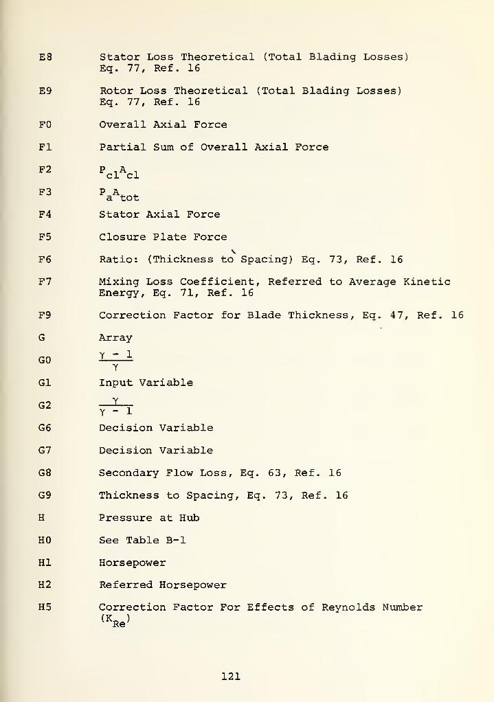
E8 Stator Loss Theoretical (Total Blading Losses)Eq. 77, Ref. 16
E9 Rotor Loss Theoretical (Total Blading Losses)Eq. 11, Ref. 16
FO Overall Axial Force
Fl Partial Sum of Overall Axial Force
F2 P n A ,cl cl
a tot
F4 Stator Axial Force
F5 Closure Plate Force
F6 Ratio: (Thickness to Spacing) Eq. 73, Ref. 16
F7 Mixing Loss Coefficient, Referred to Average KineticEnergy, Eq. 71, Ref. 16
F9 Correction Factor for Blade Thickness, Eq. 47, Ref. 16
G Array
GO 1^-1Y
Gl Input Variable
G2 —^rY - 1
G6 Decision Variable
G7 Decision Variable
G8 Secondary Flow Loss, Eq. 63, Ref. 16
G9 Thickness to Spacing, Eq. 73, Ref. 16
H Pressure at Hub
HO See Table B-l
HI Horsepower
H2 Referred Horsepower
H5 Correction Factor For Effects of Reynolds Number(KRe>
121

H6 Correction Factor For Blade Thickness (K. ) Eq. 47,Ref. 16
H8 Density Appendix B, Ref. 5
H9 Reynolds Number of Rotor, Table B-2, Ref. 5
I First Point (Used in Tabulation Program)
10 Ratio: Non-Dimensional Pressures At Various TapLocations In Stator (Fig. 5) - DO in Table B-l
II Ratio: Non-Dimensional Pressures at Various TapLocations In Stator (Fig. 5) - Dl in Table B-l
12 Ratio: Non-Dimensional Pressures At Various TapLocations In Stator (Fig. 5) - D2 in Table B-l
13 Ratio: Non-Dimensional Pressures At Various TapLocations In Stator (Fig. 5) - D3 in Table B-l
14 Ratio: Non-Dimensional Pressures At Various TapLocations In Stator (Fig. 5) - D4 in Table B-l
15 Ratio: Non-Dimensional Pressures At Various TapLocations In Stator (Fig. 5) - D5 in Table B-l
16 Ratio: Non-Dimensional Pressures At Various TapLocations In Stator (Fig. 5) - D6 in Table B-l
17 Ratio: Non-Dimensional Pressures At Various TapLocations In Stator (Fig. 5) - D7 in Table B-l
18 Ratio: Non-Dimensional Pressures At Various TapLocations In Stator (Fig. 5) - D8 in Table B-l
19 Ratio: Non-Dimensional Pressures At Various TapLocations In Stator (Fig. 5) - D9 in Table B-l
J Mach # At Station 9 In Stator
JO Joules Constant (778.16 Ft-lbf/BTU)
J2 See Table B-l
J4 Input Variable
J5 Profile Loss Coefficient Eq. 46, Ref. 16
J6 Velocity at Station 9 in Stator
J7 Non-Dimensional Stator Pressure
122

J8 Velocity at EX-TIP
J9 Velocity at Station 5 in Stator
K Fourth Degree Polynomial For K.E Factor (Fig. 4)
KO Viscosity (Sutherland Formula)
Kl Kinetic Energy Factor (G. E. Report)
K2 Beta (G. E. Report)
K3 K x B x h^ x PL
(KxK2xk6xQ0)
K4 Isentropic Head Coefficient Eq. a (22) , Ref . 5
K5 Slope of K. E. Curve (Newtonian Method)
K6 Area of Labyrinth
K7 K. E. Factor (Convergence)
K8 Second Degree Polynomial K (R ) For Nozzle (Fig. 5)
K9 See Table B-l
L Counter
LO X2
a2
+ (Xu2 - U2)2
Eq. A (21), Ref. 5
LI Rotor Loss Coefficient Eq. A (21) , Ref. 5
L2 Mach # At Various Pressure Tap Locations in Stator(Fig. 5)
L3 Mach # At Various Pressure Tap Locations in Stator(Fig. 5)
L4 Mach # At Various Pressure Tap Locations in Stator(Fig. 5)
L5 Mach # At Various Pressure Tap Locations in Stator(Fig. 5)
L6 Mach # At Various Pressure Tap Locations in Stator(Fig. 5)
L7 Mach # At Various Pressure Tap Locations in Stator(Fig. 5)
L8 Mach # At Various Pressure Tap Locations in Stator(Fig. 5)
123

L9 Mach # At Various Pressure Tap Locations in Stator(Fig. 5)
MO Referred Moment
Ml Mach # At Station 1
M2 Axial Mach # At Station 1
M3 Mach # At Station 2
M4 Axial Mach # At Station 2
M5 See Table B-l
M6 See Table B-l
M7 Referred Stator Moment
M8 Mach # At Exit - Tip
M9 Mach # At SS - Aft
NO See Table B-l
Nl See Table B-l
N2 See Table B-l
N3 See Table B-l
N4 See Table B-l
N5 See Table B-l
N6 See Table B-l
N7 See Table B-l
N8 See Table B-l
N9 See Table B-l
00 Incidence Loss Coefficient
01 See Table B-l
02 Velocities at Various Pressure Tap Locations InStator (Fig. 5)
03 Velocities at Various Pressure Tap Locations InStator (Fig. 5)
124

04
05
06
07
08
09
PO
PI
P2
P3
P4
P5
P6
P7
P9
QO
Ql
Q2
Q3
Q4
Q5
R
Re
Velocities at Various Pressure Tap Locations InStator (Fig. 5)
Velocities at Various Pressure Tap Locations InStator (Fig. 5)
Velocities at Various Pressure Tap Locations InStator (Fig. 5)
Velocities at Various Pressure Tap Locations InStator (Fig. 5)
Velocities at Various Pressure Tap Locations InStator (Fig. 5)
Velocities at Various Pressure Tap Locations InStator (Fig. 5)
Reference Pressure (29.92 in. Hg)
P-HOOD/P-LAB (RATIO)
o
Xul
(sin a,)]/xal
P,/P Eq. A (10) Ref. 51 ro
P2
P1/Pt
1
Pressure Ratio (P /V2 )
See Table B-l
Average Pressure At Rotor Exit
See Table B-l
See Table B-l
P /Pto' atm
See Table B-l
See Table B-l
Decision Variable
Array
Reynolds Number (Nozzle)
(Alpha Input)
(K Input)
125
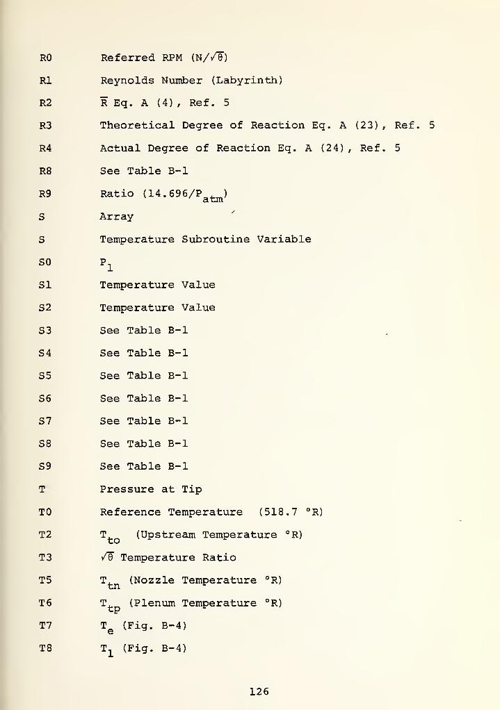
RO Referred RPM (N//6)
Rl Reynolds Number (Labyrinth)
R2 REq. A (4), Ref . 5
R3 Theoretical Degree of Reaction Eq. A (23) , Ref. 5
R4 Actual Degree of Reaction Eq. A (24) , Ref. 5
R8 See Table B-l
R9 Ratio (14 . 696/Patm )
S Array
S Temperature Subroutine Variable
50 p1
51 Temperature Value
52 Temperature Value
53 See Table B-l
54 See Table B-l
55 See Table B-l
56 See Table B-l
57 See Table B-l
58 See Table B-l
59 See Table B-l
T Pressure at Tip
TO Reference Temperature (518.7 °R)
T2 T (Upstream Temperature °R)
T3 /e" Temperature Ratio
T5 T (Nozzle Temperature °R)
T6 T (Plenum Temperature °R)
T7 Te
(Fig. B-4)
T8 Tx
(Fig. B-4)
126

T9 T2is
(Fig. B-4)
U Array
UO Mixing Loss Coefficient, Eq. 74, Ref. 16
Ul (DQ
+ Di)/48
U2 (DQ
+ Di)/48
U3 Dimensionless Velocity
U4 Dimensionless Velocity
U5 Factor %, P. 37, Ref. 16
U6 Loss Due to Tip Clearance Flow, Eq. 75, Ref. 16
U7 Tip Clearance Loss Coefficient, Referred To Isen-
tropic Conditions Eq. 76, Ref. 16
08 Pto/
pi
U9 Stator Flow Function
V Array
Tangential Rotor Velocity (V ,)VO
VI Limiting Velocity (V )
V2 V2Average Tangential Velocity Eq. A (11) , Ref. 5
V3 Val
V4 Va2
V5 V2
V6 V±
V7 Eq. A (10) , Ref. 5
V8 Stator Blockage Factor
W Array
WO Total Flow Rate (W = W - W, . )noz lab
Wl Labyrinth Flow Rate Based on K. E. Factor (G. E.Report)
127

W2 Labyrinth Convergence Flow Rate
W3 Flow Rate (ASME Equation)
W4 Ratio (WO/g)
W5 Referred Flow Rate
W6 W^^ (See Fig. B-5)
W2
(See Fig. B-5)W7
W8 W* = W, Cos {B1
- 62)
W9 W2
(See Fig. B-5)
X Array
XO Dimensionless Velocity X ,
1- Eq. A (7) , Ref . 5 (K Input)XI X
XI X , (Alpha Input)
X2 X = X + X2
u2 a
X3 1/A PdA
X4 X2
Eq. A (7) , Ref. 5
X5 X^ Eq. A (15) , Ref. 5
X6 X2
X7 R/PtQA (Alpha Input)
X8 Y(2K-1) + 1
X9 Denominator of Eq. 63, Ref. 16
Y Array
HiYO / 1 "Cp^-) y For 10
to
Yl / 1 -(^— ) y For IIto
1EPY2 / 1 "Cn 1-) Y For I2
V to
128

F-/ (f-) Y For 13to
/Y4 / 1 - (-£-) Y For 14Fto
A7 P HiY5 ^ / 1 CpM Y For 15
/ V *to
F P SY6 / 1 - (=£-) Y For 16
to
/—p—ET
I 1 - C~-) Y For 17to
/P 1^
Y8 /l - (^—) Y For 18to
P Izi1
Y9 /l - (——) Y For 19to/
Z Array
ZO CI Eq. A (8a) , Ref. 5
Zl Stator Loss Coefficient
Z2 C2 Eq. A (16) , Ref. 5
Z3 Rotor Loss Coefficient Eq. A (21) , Ref. 5
Z6 Non-Dimensional Pressure At Exit - Hub
Z7 Loss Due Tip Clearance, Eq. 75, Ref. 16
Z8 Rotor Loss Coefficient (Other Factors)
129

PRDGRRM
:
: 1:able b- 3
RRR
5IMPLE VRRIRBLE
SUBSCRIPT
¥ i 2 1 H E 6 7 9 a
H
E
C
D
E
F
E XH
-
1
J
K
L
M
N
D
P XQ
R •X
5
T
U
V s\w
X
Y
Z
5CDRE SHEET: RECDRD DF VRRIRBLE5 USED.
130
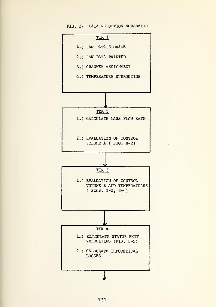
FIG. B-l DATA REDUCTION SCHEMATIC
TTR 1
1.) RAW DATA STORAGE
2.) RAW DATA PRINTED
3.) CHANNEL ASSIGNMENT
4.) TEMPERATURE SUBROUTINE
\t
TTR 2
1.) CALCULATE MASS FLOW RATE
2.) EVALUATION OF CONTROLVOLUME A ( FIG. B-2)
* r
TTR 3
1.) EVALUATION OF CONTROLVOLUME B AND TEMPERATURES( FIGS. B-3, B-4)
* '
TTR 4
U) CALCULATE STATOR EXITVELOCITIES (FIG. B-5)
2.) CALCULATE THEORETICALLOSSES
i
I
131

FIG. B-l DATA REDUCTION SCHEMATIC
J,
TTR 5
1.) PRINT REDUCED DATA
\f
TTR 6
1.) STORE REDUCED DATA
> f -1
TTR 7
1.) TABULATION OF RAW DATA
v /
TTR 8
I.) TABULATION OF REDUCED DATi
132

FIGURE B-2 CONTROL VOLUME a
STATOR
FIGURE B-3 CONTROL VOLUME b
133

FIGURE B-4 THERMODYNAMIC PROCESS OF FLUID
IN AN AXIAL TURBINE STAGE
134
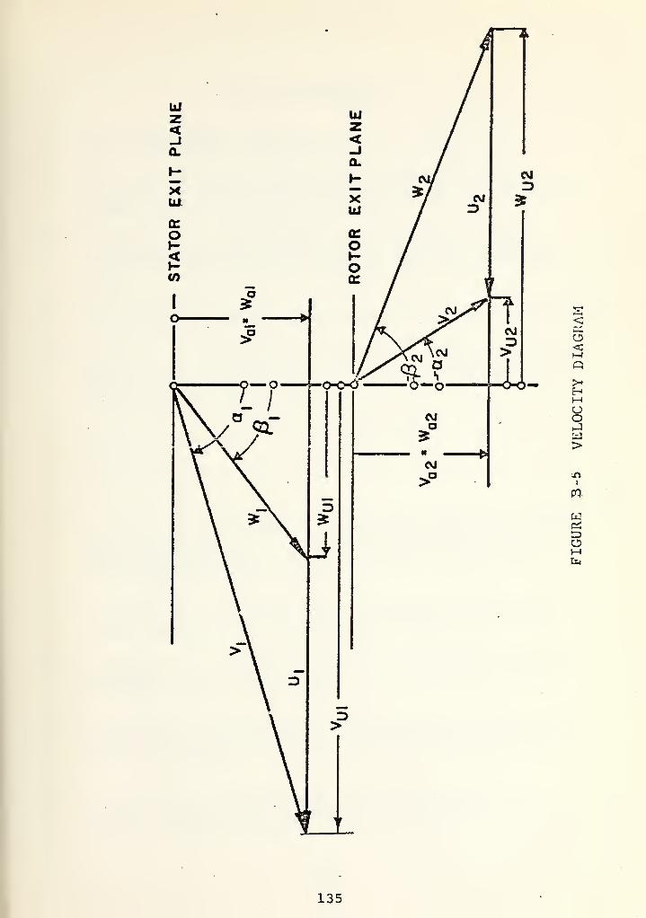
<
H1-1
o
>
i
8Mfa
135

LIST OF REFERENCES
1. Flow Measurement , Chapter 4, Part , Supplement to ASMEPower Test Codes, ASME, 1959.
2. Naval Postgraduate School Report, NPS-57SF37071A,Calibration of Flow Nozzle Using Traversing Pitot-StaticProbes , by R. P. Shreeve, July 1973.
3. Shreeve, R. P., Estimation of the Rotor-Face InletConditions and Blockage Factor for the General AtomicCorp. Helium Compression . Memo GA-RPS7405-1, February1973.
4. Hewlett-Packard 9830A, Model 30, Operating and Programming ,
Hewlett-Packard Part Number 09830-90001, January 1973.
5. Solms, W. R. , Measurement of Stage and Blade Row Perfor-mances of Axial Turbines with Subsonic and SupersonicStator Exit Condition , M. S. A. E. Thesis, NavalPostgraduate School, Monterey, California, 1975.
6. Schlichting, H., Boundary Layer Theory , P. 572-581,McGraw Hill, 1968.
7. General Electric, Duct System , Section 405.7, P. 1-15,October, 1973.
8. Commons, P.M., Instrumentation of the Transonic TurbineTest Rig To Determine The Performance of Turbine InletGuide Vanes by the Application of the Momentum andMoment of Momentum Equations , M.S.A.E. Thesis, NavalPostgraduate School, Monterey, California, 1967.
9. Lenzini, M. J., Calibration of Turbine Test Rig withImpulse Turbine at High Pressure Ratios , A.E. Thesis,Naval Postgraduate School, Monterey, California 1968.
10. Esdaile, S. G. , An Investigation of a Transonic TurbineTest Rig , M.S.A.E. Thesis, Naval Postgraduate School,Monterey, California 1969.
11. DeThomas, J. B., On-Line Data Acquisition and Instrumen-tation Improvements for the Transonic Turbine Test Rig ,
M.S.A.E. Thesis, Naval Postgraduate School, Monterey,California 1972.
12. Donovan, S. J., Performance of a High Pressure RatioImpulse Turbine With a Converging Nozzle , M.S.A.E.Thesis, Naval Postgraduate School, Monterey, California1973.
136
13. Naval Postgraduate School Report, NPS-57Va7209lA, ADescription of the Turbopropulsion Laboratory in theAeronautics Department at the Naval PostgraduateSchool , by M.H. Vavra and R.P. Shreeve, September 1972.
14. Stearns, R. F., and others, Flow Measurement withOrifice Meters , P. 65-212, D. Van Norstrand, 1951.
15. Andrews, J. and others, Turbine Test Rig Data, NavalPostgraduate School Turbopropulsion Laboratory , reportsubmitted as partial fulfillment of the requirementsfor Course No. AE 4831, Monterey, California, March,1974.
16. Vavra, M. H., Axial Turbine Design Data , Report 1174VA1,M.H. Vavra, (consultant) , Pebble Beach, California,November , 1974.
17. Vavra, M. H. , Aero-Thermodynamics and Flow in Turbo-machines , Wiley, 1960.
18. Vavra, M. H., Estimated Performance of Main Circulator ,
Report GA-1074VA2, M.H. Vavra, (consultant), PebbleBeach, California, October, 1974.
19. Vavra, M.H., Axial Flow Turbines , Lecture Series 15,Von Karman Institute for Fluid Dynamics, Brussels,1969.
137

INITIAL DISTRIBUTION LIST
No. Copies
1. Defense Documentation Center 2
Cameron StationAlexandria, Virginia 22314
2. Library, Code 0212 2
Naval Postgraduate SchoolMonterey, California 93940
3. Chairman, Department of Aeronautics 1Naval Postgraduate SchoolMonterey, California 93940
4. Associate Professor R.P. Shreeve, Code 57SfDepartment of AeronauticsNaval Postgraduate SchoolMonterey, California 93940
5. Mr. J. E. Hammer, Code 57 1Department of AeronauticsNaval Postgraduate SchoolMonterey, California 93940
6. Turbopropulsion Laboratory 12Department of AeronauticsNaval Postgraduate SchoolMonterey, California 93940
7. Lt. E. F. Robbins, USN 1VQ-2 NAVSTA ROTARota, SpainF.P.O. New York 09540
138

thesR5915
3 2768 001 95887 9DUDLEY KNOX LIBRARY