determination of genetic coefficients from field crop
TRANSCRIPT

DETERMINATION OF GENETIC COEFFICIENTS FROM FIELD
EXPERIMENTS FOR CERES-MAIZE AND SOYGRO
CROP GROWTH MODELS
A DISSERTATION SUBMITTED TO THE GRADUATE DIVISION OF THE UNIVERSITY OF HAWAII IN PARTIAL FULFILLMENT OF THE
REQUIREMENTS FOR THE DEGREE OF
DOCTOR OF PHILOSOPHY
IN
AGRONOMY AND SOIL SCIENCE
MAY 1995
By
Richard M. Ogoshi
Dissertation Committee:
Goro Uehara, Chairman Duane Bartholomew
Robert Caldwell Kent Kobayashi Douglas Friend

11
We certify that we have read this dissertation and that, in our opinion, it is
satisfactory in scope and quality as a dissertation for the degree of Doctor
of Philosophy in Agronomy and Soil Science.
DISSERTATION COMMITTEE
y c T U ) .Chairman r—'
C U U &
^ J * .

ACKNOWLEDGMENTS
Over the life of this project many people contributed to the completion and
integrity of this work, and the well-being of the author. Dr. Goro Uehara exercised
great patience and gave invaluable advice for this research work. Dr. Gordon Tsuji
was instrumental in executing the experiment with his administrative and
psychological expertise. The IBSNAT project staff cheerfully gave valuable support:
Valentine Ah Loy, Pam Brooks, Horatio Chan, Ada Chu, Tony Denault, Lori Higa,
Daniel Imamura, Connie Kerley, Earl Kim, Richard and Teri Jacintho, Luis
Manrique, Robbie Melton, Karen Nakama, Sue Sakumoto, Susan Sato, Agnes
Shimamura, and Agatha Tang. Dr. L. Anthony Hunt gave crucial direction and
impetus to this entire project. The dissertation committee provided astute suggestions
that made this work scientific and comprehendible: Drs. Duane Bartholomew, Robert
Caldwell, Douglas Friend, and Kent Kobayashi. Fellow graduate students were
helpers and commiserators; Hui Feng Chang, Phoebe Kilham, Hemant Prasad, and
Surya Tewari. The NifTAL Project and Kula Experiment Station extended gracious
cooperation with land, equipment, and labor. The U.S. Agency for International
Development generously lent financial support. Pioneer Hibred International and Dr.
Randall Nelson, USD A, courteously provided seed. My family and friends provided
constant encouragement and prayers. My mother and father believed without seeing.
To all these fine people, I extend my deepest appreciation.
Ill
IV
ABSTRACT
Lack of genetic coefficients is a reason crop models are not widely used. A
project was therefore developed to evaluate a field method to calculate genetic
coefficients for crop models.
The phenology models fi-om SOYGRO v. 5.42 and CERES-Maize v. 2.1, with
the existing genetic coefficients, were tested using data for soybean and maize grown
under extreme photoperiods. Identical experiments were performed at two sites on
Maui Island, Hawaii, over three years. The treatment design was a factorial of
photoperiods (natural, natural + 0.5 h, 14-, 17-, and 20-h) and cultivars ('Bragg',
'Evans', 'Jupiter', and 'Williams' for soybean and Pioneer hybrids X304C, 3165, 3324,
3475, and 3790 for maize). Observations included development stage dates, yield,
yield components, aboveground biomass weight, soil chemical analysis, and weather.
Comparisons between observed and simulated results showed that soybean and maize
development was well simulated. However, soybean yield and maize growth and
yield were not well simulated. Further analysis suggested that model bias and
parameter uncertainty accounted for nearly equal proportions of variation in soybean
grain yield, whereas most maize growth and yield variation was due to model bias.
SOYGRO and CERES-Maize genetic coefficients were calculated from the
data in the above experiments. One method to recalculate genetic coefficients was to
incrementally change the genetic coefficients until simulated matched observed

results. Another method was performed according to the maize modeler's suggestion.
The fitting method adequately established development genetic coefficients, whereas
growth coefficients had similar biases as the original genetic coefficients. The
explicit method did not well simulate maize growth.
Using the fitted genetic coefficient means ± standard error, a sensitivity
analysis was done. The genetic coefficient error that caused the greatest variation in
simulated yield and aboveground biomass was identified. The most problematic
genetic coefficients and associated model routines for yield and growth was the pod
production relationship to nightlength in SOYGRO and juvenile phase duration in
CERES-Maize.
V
TABLE OF CONTENTS
Acknowledgements........................................................................................................... iiiAbstract............................................................................................................................... ivList o f Tables................................................................................................................... viiiList o f Figures.................................................................................................................. xiiiChapter 1: Review of Literature........................................................................................ 1
Introduction..............................................................................................................1Genetic control of crop development and grow th...............................................2Interaction of genotype and environment on crop development and growth . . 8
Physiology of environmental effects on crop development and growth . . . . 14SOYGRO and CERES-Maize description.........................................................28Genetic coefficients in crop models...................................................................31Determining genetic coefficients....................................................................... 34
Chapter 2: Simulating soybean and maize development and growth underextreme artificial photoperiods with SOYGRO and CERES-Maize cropsimulation m odels............................................................................................... 36Introduction.......................................................................................................... 36Methods and materials.........................................................................................37Results................................................................................................................. 49Discussion........................................................................................................... 84
Chapter 3: Evaluating methods to estimate genetic coefficients in SOYGROand CERES-Maize.............................................................................................98Introduction.........................................................................................................98Methods and materials.....................................................................................101Results................................................................................................................110Discussion.........................................................................................................203
Chapter 4: Sensitivity analysis of derived genetic coefficients for SOYGROand CERES-Maize...........................................................................................207Introduction.......................................................................................................207Methods and materials.................................................................................... 208Results............................................................................................................... 216Discussion.........................................................................................................227
Chapters: Summary and conclusion.........................................................................240Appendix A: Soybean data, summer 1988 ................................................................ 243Appendix B: Soybean data, winter 1988 .................................................................. 263Appendix C: Soybean data, summer 1989................................................................ 271Appendix D: Soybean data, summer 1990................................................................ 291Appendix E: Maize data, summer 1988 ................................................................... 311Appendix F: Maize data, winter 1988 ........................................................................331Appendix G: Maize data, summer 1989 ................................................................... 339
VI

Vll
Appendix H: Maize data, summer 1990 ................................................................... 359Appendix I: Maize data, winter 1990...................................................................... 379Appendix J: Weather da ta ..........................................................................................387References.....................................................................................................................433

LIST OF TABLESTable Page
1. Genetic coefficients of soybean cuitivars for SOYGRO v.5.42........................ 44
2. Genetic coefficients of Pioneer hybrids for CERES-Maize v.2.1 ......................45
3. Mean squares from analyses of variance for number of nodes onmainstem and days from planting to flowering for soybean...............................50
4 . Mean squares from analyses of variance for grain weight plant’',seeds plant’*, and seed weight for soybean........................................................... 54
5 . Mean squares from analysis of variance for total leaf number in m aize 58
6 . Mean squares from analysis of variance for days to silking in m aize................61
7. Mean squares from analyses of variance for grain weight plant’’,kernel number plant’', and single kernel weight in m aize................................63
8 . Regression and error analysis for SOYGRO phenology using original genetic coefficients................................................................................................ 69
9. Regression and error analysis for SOYGRO growth using originalgenetic coefficients.................................................................................................7 3
10. Regression and error analysis for CERES-Maize development usingoriginal genetic coefficients...................................................................................80
11. Regression and error analysis for CERES-Maize growth usingoriginal genetic coefficients...................................................................................85
12. Developmental and growth genetic coefficients in SOYGRO........................ 99
13. Developmental and growth genetic coefficients in CERES-Maize............... 100
14. Original and fitted SOYGRO genetic coefficients for cuitivars 'Bragg'and 'Evans'.............................................................................................................I l l
15. Original and fitted SOYGRO genetic coefficients for cuitivars'Jupiter' and 'W illiams'......................................................................................... 112
• Vlll

Tablg16. Original, explicit, and fitted CERES-Maize genetic coefficients for
Pioneer hybrids X304C and 3165.......................................................................114
17. Original, explicit, and fitted CERES-Maize genetic coefficients forPioneer hybrids 3324 and 3475 ......................................................................... 114
18. Original, explicit, and fitted CERES-Maize genetic coefficients forPioneer hybrid 3790 ............................................................................................. 115
19. Mean squares firom analyses of variance for fitted SOYGRO genetic coefficients PHTHRS(l), PHTHRS(2), and PHTHRS(4)............................... 118
20. Mean squares fi'om analyses of variance for fitted SOYGRO genetic coefficients VARTH, VARNl, and VARNO.....................................................121
21. Mean squares tfom analyses of variance for fitted SOYGRO genetic coefficients PHTHRS(6 ), PHTHRS(7), and PHTHRS(8 ) ............................... 123
22. Mean squares from analyses of variance for fitted SOYGRO genetic coefficients PHTHRS(9) and PHTHRS(IO)......................................................124
23. Mean squares from analyses of variance of fitted SOYGRO genetic TRIFOL for soybean cultivars 'Bragg' and 'Evans'........................................... 130
24. Mean squares from analyses of variance for fitted SOYGRO genetic coefficients SIZELF and SLA V A R ....................................................................131
25. Mean squares from analyses o f variance for fitted SOYGRO genetic coefficients SDPDVR, FLWMAX, and PODVAR.......................................... 133
26. Mean squares from analyses of variance for fitted SOYGRO genetic coefficients SHVAR, SDVAR, and PHFAC3...................................................134
27. Mean squares from analyses of variance for explicit CERES-Maizegenetic coefficients PI and P 5 ............................................................................ 136
28. Mean squares from analysis of variance for explicit CERES-Maizegenetic coefficient P 2 ........................................................................................... 139
IX

la h le Pqgg29. Mean squares from analyses of variance for explicit CERES-Maize
genetic coefficients G2 and G 3 ........................................................................... 142
30. Mean squares from analyses of variance for fitted CERES-Maizegenetic coefficients PI and P 5 ............................................................................ 146
31. Mean squares from analysis of variance for fitted CERES-Maizegenetic coefficient P I ........................................................................................... 149
32. Mean squares from analyses of variance for fitted CERES-Maizegenetic coefficients G2 and G 3 ........................................................................... 153
33. Mean squares from analysis of variance for fitted CERES-Maizecrop coefficient P 9 .............................................................................................. 157
34. Mean squares from analyses of variance for fitted CERES-Maizecrop coefficients XLPGDD and PCHRON...................................................... 159
35. Regression and error analysis comparing control and naturalphotoperiod treatments for soybean development............................................. 164
36. Regression and error analysis comparing control and naturalphotoperiod treatments for soybean growth.....................................................165
37. Regression and error analysis comparing control and naturalphotoperiod treatments for maize development................................................167
38. Regression and error analysis comparing control and naturalphotoperiod treatments for maize growth.........................................................168
39. Regression and error analysis of simulated soybean developmentusing fitted genetic coefficients.........................................................................170
40. Regression and error analysis of simulated soybean growth usingfitted genetic coefficients................................................................................... 174
41. Regression and error analysis of simulated maize development using explicit genetic coefficients............................................................................... 181
X
Table Page42. Regression and error analysis of simulated maize development using
fitted genetic coefficients....................................................................................185
43. Regression and error analysis of simulated maize growth using fitted genetic coefficients.............................................................................................. 189
44. Regression and error analysis of simulated maize growth usingexplicit genetic coefficients................................................................................ 195
45. Mean and standard error of 16 SOYGRO genetic coefficients forsoybean cultivars 'Bragg' and 'Evans'................................................................ 211
46. Mean and standard error of 16 SOYGRO genetic coefficients forsoybean cultivars 'Jupiter' and 'Williams'..........................................................212
47. Mean and standard error of five CERES-Maize genetic coefficientsand three variables for Pioneer hybrids X304C, 3165, and 3324.................. 214
48. Mean and standard error of five CERES-Maize genetic coefficientsand three variables for Pioneer hybrids 3475 and 3790..................................215
49. Sums of squares for yield of 'Bragg' soybean.................................................. 217
50. Sums of squares for yield of 'Evans' soybean.................................................. 218
51. Sums of squares for yield of 'Jupiter' soybean................................................. 219
52. Sums o f squares for yield of'Williams' soybean...............................................220
53. Sums of squares for aboveground biomass weight of 'Bragg'soybean................................................................................................................. 2 2 1
54. Sums of squares for aboveground biomass weight of 'Evans'soybean................................................................................................................. 2 2 2
55. Sums of squares for aboveground biomass weight of 'Jupiter'soybean................................................................................................................. 223
56. Sums of squares for aboveground biomass weight of'Williams'soybean................................................................................................................. 224
XI
Tabk Page57. Sums of squares for grain yield of Pioneer hybrid X304C m aize..................228
58. Sums of squares for grain yield of Pioneer hybrid 3165 m aize.................... 228
59. Sums of squares for grain yield of Pioneer hybrid 3324 m aize.................... 229
60. Sums of squares for grain yield of Pioneer hybrid 3475 m aize.................... 229
61. Sums of squares for grain yield of Pioneer hybrid 3790 m aize.................... 230
62. Sums of squares for aboveground biomass weight of Pioneer hybridX304C m aize........................................................................................................230
63. Sums of squares for aboveground biomass weight of Pioneer hybrid3165 m aize............................................................................................................ 231
64. Sums of squares for aboveground biomass weight of Pioneer hybrid3324 m aize............................................................................................................ 231
65. Sums of squares for aboveground biomass weight of Pioneer hybrid3475 m aize............................................................................................................ 232
6 6 . Sums of squares for abovegroimd biomass weight of Pioneer hybrid3790 m aize............................................................................................................ 233
XII

LIST OF FIGURESFisurg
1. Photoperiod extension effect on number of main stem nodes in soybean . . . 51
2. Photoperiod extension effect on days to flowering in soybean........................52
3. Photoperiod extension effect on grain yield plant'' in soybean........................55
4. Photoperiod extension effect on seed number plant' in soybean.....................56
5. Photoperiod extension effect on single seed weight in soybean.......................57
6 . Photoperiod extension effect on total leaf number in m aize........................... .60
7. Photoperiod extension effect on days to silking in m aize.................................62
8 . Photoperiod extension effect on grain yield plant' in m aize............................ 64
9. Photoperiod extension effect on kernel weight in m aize...................................65
10. Photoperiod extension effect on kernels plant' in m aize..................................67
11. Observed vs. simulated plot of days to flowering for soybean using original genetic coefficients................................................................................70
12. Observed vs. simulated plot of days to full pod for soybean usingoriginal genetic coefficients................................................................................71
13. Observed vs. simulated plot o f days to physiological maturityfor soybean using original genetic coefficients..................................................72
14 . Observed vs. simulated plot of grain yield for soybean using originalgenetic coefficients............................................................................................... 74
15. Observed vs. simulated plot of single seed weight for soybean using original genetic coefficients.................................................................................75
16. Observed vs. simulated plot of seed number for soybean using originalgenetic coefficients...............................................................................................76
X lll

Fisprg Page17. Observed vs. simulated plot of aboveground biomass weight for
soybean using original genetic coefficients.........................................................78
18. Observed vs. simulated plot of stem weight for soybean using original genetic coefficients................................................................................................ 79
19. Observed vs. simulated plot of tassel initiation for maize usingoriginal genetic coefficients...................................................................................81
20. Observed vs. simulated plot of silking for maize using originalgenetic coefficients.................................................................................................82
21. Observed vs. simulated plot of physiological maturity for maizeusing original genetic coefficients........................................................................83
22. Observed vs. simulated plot of grain yield for maize using originalgenetic coefficients.................................................................................................8 6
23. Observed vs. simulated plot of single kernel weight for maizeusing original genetic coefficients........................................................................87
24. Observed vs. simulated plot of number of kernels for maize usingoriginal genetic coefficients....................................................................... ; . . . 8 8
25. Observed vs. simulated plot of abovegroimd biomass weight formaize using original genetic coefficients............................................................ 89
26. Observed vs. simulated plot o f stover weight for maize usingoriginal genetic coefficients................................................................................. 90
27. Photoperiod extension effect on estimating PHTHRS(2) genetic coefficient for SOYGRO....................................................................................120
28. Photoperiod extension effect on estimating PHTHRS(6 ) genetic coefficient for SOYGRO....................................................................................125
29. Photoperiod extension effect on estimating PHTHRS(7) genetic coefficient for SOYGRO....................................................................................126
XIV

Figurg30. Photoperiod extension effect on estimating PHTHRS(8 ) genetic
coefficient for SOYGRO....................................................................................127
31. Photoperiod extension effect on estimating PHTHRS(9) geneticcoefficient for SOYGRO....................................................................................128
32. Photoperiod extension effect on estimating PHTHRS( 10) geneticcoefficient for SOYGRO....................................................................................129
33. Photoperiod extension effect on estimating SIZELF geneticcoefficient for SOYGRO....................................................................................132
34. Year effect on estimating explicit PI genetic coefficient forCERES-Maize.....................................................................................................138
35. Photoperiod effect on estimating explicit P5 genetic coefficientfor CERES-Maize................................................................................................140
36. Photoperiod effect on estimating explicit G2 genetic coefficientfor CERES-Maize................................................................................................143
37. Photoperiod effect on estimating explicit G3 genetic coefficientfor CERES-Maize................................................................................................144
38. Year effect on estimating fitted PI genetic coefficient forCERES-Maize......................................................................................................147
39. Photoperiod effect on estimating fitted P5 genetic coefficient forCERES-Maize......................................................................................................148
40. Photoperiod effect on estimating fitted P2 genetic coefficient forCERES-Maize...................................................................................................... 150
41. Effect of decreased threshold photoperiod on fitted P2 values....................... 151
42. Photoperiod effect on estimating fitted G2 genetic coefficient forCERES-Maize...................................................................................................... 154
43. Photoperiod effect on estimating fitted G3 genetic coefficient forCERES-Maize...................................................................................................... 155
XV

Figure44. Year effect on estimating fitted P9 crop coefficient for
CERES-Maize...................................................................................................... 158
45. Photoperiod effect on estimating fitted XLPGDD crop coefficientfor CERES-Maize................................................................................................160
46. Photoperiod effect on estimating fitted PCHRON crop coefficientfor CERES-Maize................................................................................................162
47. Observed vs. simulated plot of days to flowering for soybean usingfitted genetic coefficients....................................................................................171
48. Observed vs. simulated plot of days to full pod for soybean usingfitted genetic coefficients....................................................................................172
49. Observed vs. simulated plot of days to physiological maturity forsoybean using fitted genetic coefficients.......................................................... 173
50. Observed vs. simulated plot of grain yield for soybean using fittedgenetic coefficients..............................................................................................175
51. Observed vs. simulated plot of weight seed*' for soybean usingfitted genetic coefficients...................................................................................176
52. Observed vs. simulated plot of seeds m’ for soybean using fittedgenetic coefficients............................................................................................ 177
53. Observed vs. simulated plot o f aboveground biomass weight forsoybean using fitted genetic coefficients......................................................... 178
54. Observed vs. simulated plot of stem weight for soybean using fitted genetic coefficients............................................................................................ 179
55. Observed vs. simulated plot of days to tassel initiation for maizeusing explicit genetic coefficients.....................................................................182
56. Observed vs. simulated plot of days to silking for maize usingexplicit genetic coefficients................................................................................183
XVI

XVll
Figure Page57. Observed vs. simulated plot of days to physiological maturity for
maize using explicit genetic coefficients......................................................... 184
58. Observed vs. simulated plot of days to tassel initiation for maizeusing fitted genetic coefficients....................................................................... 186
59. Observed vs. simulated plot of days to silking for maize using fitted genetic coefficients..............................................................................................187
60. Observed vs. simulated plot of days to physiological maturity formaize using fitted genetic coefficients..............................................................188
61. Observed vs. simulated plot of grain yield for maize using explicitgenetic coefficients............................................................................................. 190
62. Observed vs. simulated plot of single kernel weight for maize using explicit genetic coefficients................................................................................191
63. Observed vs. simulated plot of kernels m‘ for maize using explicitgenetic coefficients............................................................................................. 192
64. Observed vs. simulated plot of aboveground biomass weight formaize using explicit genetic coefficients.......................................................... 193
65. Observed vs. simulated plot of stover weight for maize using explicit genetic coefficients............................................................................................. 194
66. Observed vs. simulated plot o f grain yield for maize using fittedgenetic coefficients............................................................................................. 196
67. Observed vs. simulated plot of single kernel weight for maize usingfitted genetic coefficients................................................................................... 197
6 8 . Observed vs. simulated plot of kernels m’ for maize using fittedgenetic coefficients............................................................................................. 198
69. Observed vs. simulated plot of aboveground biomass weight formaize using fitted genetic coefficients............................................................. 199

XVlll
Eigiire Page70. Observed vs. simulated plot of stover weight for maize using fitted
genetic coefficients............................................................................................. 2 0 0
71. Approximate relationship between pod production nightlength factorand nightlength for 'Bragg' soybean................................................................. 236
CHAPTER 1
REVIEW OF LITERATURE
Introduction
One approach to efficiently produce crops is to match crop requirements to
land characteristics. Crop development and growth depend on land characteristics
such as temperature, solar radiation, photoperiod, rainfall, and soil nutrients. Weather
factors are especially variable among years. To characterize crop production at a
location, the effect of the variable weather on crop yield must be recognized. A
whole probability distribution on yield can be used to assess crop production because
the shape of the disribution characterizes the risk of crop failure. Developing the
probability distribution requires observing yield over many years so that a wide range
of weather has affected the crop. In addition, probability distributions for each
genotype need defining since genotypes differently respond to environment. A
quicker method to develop the probability distribution is to use crop simulation
models. Crop simulation models can define whole probability distributions because
they quantify environment-by-genotype interactions. After estimating the risk of crop
failure from the probability distributions, the crop and genotype suited for the land
area can be selected.
Some crop models were developed to quickly assess the crop production
potential under specified management practices for different locations. Simulation

models were designed to account for genotype response to major environmental
factors. The basis for these responses came from research in disciplines such as
meteorology, soil science, plant physiology, agronomy, and plant breeding. These
responses were converted to equations that described growth and development. With
this description of plant response to its environment, the modeled factors are
manipulated to find better management practices or location.
Crop models simulate genotype-by-environment interactions based on
physiological principles. Genes control plant growth and development. The genetic
potential for growth and development is modified by environmental conditions and
results in genotype-by-environment interactions. The genotype-environment
interactions can be simplified if physiological principles are known. The
physiological principles can explain the genotype-by-environment interaction. The
following review of published literature shows these connections between genetics,
genotype-environment interaction, and plant physiology and its application to
modeling crop growth and development.
Genetic Control of Crop Development and Growth
Development and growth of soybean and maize depend on the genetic
constitution of the plant. Genes are known to control photoperiodism, phase duration,
yield, yield components, and seed growth rate in both crops.
Five loci have been found to control photoperiod sensitivity of flowering and
2

maturation in soybean: namely E,, Ej, E3 , E4 , and E, (Saindon et al., 1989b). The five
loci have two alleles each. Alleles E,, Ej, E3 (McBlain et al., 1987), E4 (Saindon et
al., 1989a; Saindon et al., 1990), and E5 (McBlain and Bernard, 1987) were
responsible for photoperiod sensitivity that caused late flowering and late maturation
under long photoperiod. In addition, the alleles e„ ej, e3 , e4 , and generally did not
affect photoperiod response. Partially dominant gene action (i.e., an intralocus action
where heterozygous progeny's phenotype was between the parents but closer to one or
the other) was exhibited at loci Ej (Saindon et al., 1990), Ej and Ej (McBlain and
Bernard, 1987). Dominant gene action, an intralocus action that gives heterozygous
progeny's phenotype the same as the homozygous dominant parent, occurred at loci
E3 and E4 (Saindon et al., 1989a), The photoperiod sensitive alleles E,, Ej, E3 , E4 , and
E5 were dominant to the photoperiod insensitive alleles e,, ej, e3 , e4 , and ej
Interactions among alleles, known as epistasis, accounted for a large range of
photoperiod sensitivities observed in soybean cultivars. Epistatic interaction occurred
between loci E, and E4 (Saindon et al., 1990). In the presence of allele E4 , allele E,
delayed flowering and maturity more than twice as long than its effect in the presence
of allele e4 . Similarly, in the presence of Ej, E4 delayed flowering and maturity more
than twice than its effect in the presence of allele e,. Other epistatic interactions
occurred with alleles Ej, Ej, and E3 (McBlain et al., 1987). The delay in flowering
was greater for allele E 3 when E, and Ej were present. Saindon et al. (1989b)
deduced that allele E4 had epistatic interaction with other unidentified maturation
3

alleles. Thus, these five known loci accounted for most of the variation in soybean
photoperiod sensitivity (McBlain and Bernard, 1987; Saindon et al., 1989b; Saindon
et al., 1990) and adaptability to a wide range of latitudes.
The response of days to anthesis to photoperiod in maize is under control of
several loci. Photoperiod response has been documented as a fimction of three
parameters: basic vegetative phase, maximum optimal photoperiod, and photoperiod
sensitivity (Rood and Major, 1981). Basic vegetative phase was defined as the time
to anthesis under optimum photoperiod. Maximum optimal photoperiod was the
longest photoperiod that did not delay time to anthesis. Photoperiod sensitivity was
the time anthesis delayed per hour of photoperiod beyond the maximum optimal
photoperiod. The basic vegetative phase was shown to be under partial dominant
gene action where short basic vegetative phase was dominant to long (Rood and
Major, 1981). The gene action for maximum optimal photoperiod was variable and
no conclusions were made (Rood and Major, 1981). Photoperiod sensitivity was
observed to be under control of several loci (Brewbaker, 1981; Russell and Stuber,
1983) with additive gene action (Brewbaker, 1981; Russell and Stuber, 1983; Russell
and Stuber, 1985), basically interlocus action among several loci where an allele at
each locus added or subtracted a unit of phenotypic value. Broad sense heritabilities
(i.e., the proportion of phenotypic variation due to genetics of all gene action types)
were very high for the three parameters. Heritability was 96.5% for basic vegetative
phase, 70.8% for maximum optimal photoperiod, and 70.6% (Rood and Major, 1981)
4

or 94.7% (Brewbaker, 1981) for photoperiod sensitivity. Therefore, photoperiod
response in maize was mainly under genetic control.
Genes control the time between two developmental stages (i.e., a phase) in
soybean. The genes that control flowering in soybean similarly control maturation.
Flowering and maturation is controlled by non-additive gene action with non-additive
interaction between alleles (McBlain and Bernard, 1987). Other evidence for the
genetic control of phases came from heritability studies. The results of these broad
sense heritability studies showed that most of the phenotypic variation was under
genetic control. In soybean experiments conducted across locations and years, broad
sense heritability for days to flowering ranged from 71 to 91% and for days to
maturity from 71 to 87% (Chan et al., 1986; Kwon and Torrie, 1964; Bartley and
Weber, 1952; Anand and Torrie, 1963; Johnson et al., 1955). The reproductive phase
from flowering to maturity had estimated heritabilities between 43 and 82% with a
mean of 62% ( Kwon and Torrie, 1964; Bartley and Weber, 1952; Anand and Torrie,
1963; Johnson et al., 1955). Another measure of genetic control of phenotype was
narrow sense heritability. Narrow sense heritability is the proportion of phenotypic
variance attributed to additive gene action. Narrow sense heritability measures how
amenable a trait is to breeding methods because additive gene action is stable and
passed from generation to generation unlike dominance or epistatic gene action. Seed
filling phase, from beginning seed fill to physiological maturity, had heritabilities
-20% to 24% (Smith and Nelson, 1987) and 16% to 63% (Pfeiffer and Egli, 1988).
5
Thus, while soybean vegetative and reproductive phases were under genetic control,
manipulating the phases with breeding methods may be difficult for some phases
because of the low narrow sense heritability.
The phase emergence to silking and the grain filling phase was under genetic
control in maize. In a six by six diallel cross experiment over two years and two
locations, days to silk had a broad sense heritability of 96.6% and narrow sense
heritability of 68.5% (Dhillon et al., 1990). The heritability showed that gene action
was predominantly additive for days to silking. In a similar experiment, Bonaparte
(1977) found that days to silk was under additive gene action with incomplete
dominance where early silking was dominant. Furthermore, at least four genes
regulated days to silk. Grain filling period had broad sense heritability of 84.2%
(Perenzin et al., 1980) which suggests the importance of genetics over environment
for this phase. The effective grain filling period, defined as the ratio of final kernel
weight to kernel growth rate or duration of the linear kernel growth, is almost
equivalent to the grain filling period. Effective grain fill period was shown to be
under additive gene action (Ottaviano and Camussi, 1981). Two studies showed that
the effective grain filling period in progeny was much longer than either parent
demonstrating that heterosis may have occurred (Poneleit and Egli, 1979; Djisbar and
Gardner, 1989). These experiments showed that the phase emergence to silking and
grain filling phase were under genetic control.
Environment affects soybean yield and yield components more than the
6
genotype. Soybean yield per plant had a broad sense heritability of -1.7 to 67% with
a mean of 32% (Chan et al., 1986; Faluyi, 1990; Anand and Torrie, 1963; Johnson et
al., 1955; Kwon and Torrie, 1964; Bartley and Weber, 1952). The yield components
of pods per plant, seeds per pod, and seed size had broad sense heritabilities of 0 to
71%, 0 to 60%, and 44 to 92% (Bartley and Weber, 1952; Kwon and Torrie, 1964;
Johnson et al., 1955; Anand and Torrie, 1963; Chan et al., 1986; Faluyi, 1990). The
wide range in heritabilities for yield and yield components may be attributed to
differences in environment (Anand and Torrie, 1963; Chan et al., 1986) and
genotypes (Faluyi, 1990). In general, genes contributed to the phenotypic variation,
but environment was the major determinant for yield and yield components in
soybean.
Genes affect maize yield, yield components and kernel growth rate, but the
gene action was fully described for all traits. Broad sense heritability for grain yield
was shown to be 96.7% (Perenzin et al., 1980), but narrow sense heritability ranged
from 23.3% to 67.0% (Singh et al., 1989). The low narrow sense heritability showed
the gene action for yield was non-additive. The non-additive gene action for yield
had been identified as dominance in earlier experiments (Gamble, 1962a; Gamble,
1962b; Stuber et al., 1966). The yield components kernel weight, kernels per ear row,
and rows per ear had fairly low narrow sense heritabilities: 33.8 to 34.9%, 48.9%, and
28.2% (Singh et al., 1989). The low narrow sense heritabilities supported the studies
that found the yield components kernel weight and rows per ear were under dominant

gene action (Gamble, 1962b; Gamble 1962c). Contrary to these results, Russell
(1976) showed kernel weight and rows per ear were under additive gene control. The
difference in results may be attributed to the use of material that had undergone
selection for yield that imparted stability to additive effects (Gamble, 1962c). Kernel
growth rate had broad sense heritability of 97% (Perenzin et al., 1980). There are
indications that gene action for kernel growth rate may be dominant (Poneleit and
Egli, 1979), additive (Ottaviano and Camussi, 1981), and heterotic (Poneleit and Egli,
1979). The mixed results in gene action may be due to environmental effects that
influenced phenotype (Singh et al., 1989). While the gene action for yield and yield
components had been characterized as dominance, the gene action for kernel growth
rate has not been well established.
Thus, the evidence shows that genes are important contributors to phenotypic
variation in development and growth of soybean and maize. The genetics of
photoperiodism and the large broad sense heritabilities of vegetative and reproductive
phases, yield, yield components, and growth supported the importance of genetics in
phenotypic variation. However, environment substantially contributed to the
phenotypic variation and cannot be ignored.
Interaction of Genotype and Environment on Crop Development and Growth
Environment differently influences phase duration, yield, yield components,
and growth among genotypes. Environmental factors such as temperature, daylength,
8

soil moisture, and soil fertility modify development and growth among crop varieties.
The distinct environmental modification among genotypes is manifest in the
genotype-by-environment interaction in an analysis of variance.
In soybean, environment factors differently influence the time to flowering,
maturity, and flowering to maturity among cultivars. Days from planting to
flowering have been observed in field experiments that altered environment through
varying the year, location, and for planting date. The genotype-year interaction was
significant in an experiment conducted over two years and two locations (Kwon and
Torrie, 1964). The interaction was presumably caused by differences in temperature
and moisture among the years. Kaw and Madhava Menon (1978) found the
genotype-location interaction highly significant and suggested the cause was
difference in soil texture, fertility, moisture, and salinity. In a study of 8 6 cultivars
and 96 locations over three years, Schutz and Bernard (1967) found significant
genotype-year and genotype-location interactions, but the variance for
genotype-location was larger than genotype-year interaction. The genotype-planting
date interaction was found significant and attributed to differing photoperiod
sensitivity among cultivars (Pathak and Nema, 1988; Kaw and Madhava Menon,
1978). The genotype-environment interaction for time from planting to maturity was
determined from field experiments that altered environment through different
planting dates, locations, and years. In experiments where planting date was varied
over one, three, and 1 0 months, genotype-planting date interactions were significant

(Raymer and Bernard, 1988; Pathak and Nema, 1988; Kaw and Madhava Menon,
1978). Examination of the genotype-planting date interaction revealed that the
variation in time to maturity was much less for early than for the late maturing
varieties (Pathak and Nema, 1988; Raymer and Bernard, 1988). The supposed cause
of the significant interaction was different photoperiod sensitivity among genotypes
(Kaw and Madhava Menon, 1978). The phase from flowering to maturity exhibited
significant genotype-environment interaction. Kwon and Torrie (1964) showed that
location and year differently affected genotypes for this phase. In an experiment
where the genotype-planting date interaction was significant, as planting date was
delayed, the early varieties flowering to maturity phase was shortened more than the
late varieties (Pathak and Nema, 1988). Thus, environment distinctly affected the
phases emergence to flowering, emergence to maturity, and flowering to maturity
according to genotype.
Soybean yield and yield components display genotype-environment
interactions. Environment was varied in several studies by conducting the same
experiment over different years, locations, or planting. The variation in yield across
years was significantly different among genotypes, that is, the genotype-year
interaction was significant (Kwon and Torrie, 1964; Khadem et al., 1985a; Raymer
and Bernard, 1988; Kang et al., 1989). The genotype-year interaction variance was
much larger than the genotype variance (Kwon and Torrie, 1964; Schutz and Bernard,
1967) implied that yield response to environment among genotypes was greater than
10

the differences in yield among genotypes. Genotype-location interaction was found
significant for yield (Kwon and Torrie, 1964; Schutz and Bernard, 1967; Kang et al.,
1989; Kaw and Madhava Menon, 1978). Kang et al. (1989) attributed the
genotype-location interaction to differences among genotypes in their response to
fertility, cultural practices, and rainfall but not temperature or relative humidity. The
significance of the genotype-planting date interaction for yield was variable. In one
experiment the genotype-planting date interaction was significant (Konwar and
Talukdar, 1986), in two others it was not significant (Raymer and Bernard, 1988;
Kaw and Mahava Menon, 1978). Raymer and Bernard (1988) found that
genotype-planting date interactions were significant in two of three years. However,
when the experiments were combined, the genotype-planting date interaction was not
significant. Therefore, the significance and non-significance of the
genotype-planting date interaction among the different experiments may be due to
years. Nevertheless, soybean yield response to environment varies among genotypes.
The yield components number-of-pods-per-plant, number-of-seeds-per-pod,
and mass-per-100-seeds showed significant genotype-environment interactions. The
response in number-of-pods-per-plant to environment was different among genotypes
where environment was varied over years (Khadem et al., 1985b), locations (Kaw and
Madhava Menon, 1978), and planting dates (Konwar and Talukdar, 1986). Seeds per
pod also showed significant genotype-environment interaction (Konwar and
Talukdar, 1986). While 100-seed-mass was shown to have a significant
11

genotype-environment interaction (Khadem et al., 1985b; Raymer and Bernard, 1988;
Konwar and Talukdar, 1986), the magnitude of the interaction variance was smaller
than the genotype variance (Kwon and Torrie, 1964; Schutz and Bernard, 1967). The
difference in variance magnitudes indicated that the genotype effect was more
important than genotype-environment interaction in determining 1 0 0 -seed-mass.
Thus, yield component response to environment was significantly different among
genotypes.
In maize, genotype-environment interactions are significant for
photoperiodism, phase durations, yield, and yield components. The significant
interactions demonstrated that genotypes responded differently to their environment.
Photoperiod sensitivity displays significant genotype-environment interaction
in maize. Photoperiod sensitivity, measured as days to tassel initiation or total leaf
number, has shown significant genotype-environment interaction in multi-location
experiments (Russell and Stuber, 1985; Russell and Stuber, 1983a). Photoperiod
sensitivity decreased as temperature increased (Hunter et al., 1974; Russell and
Stuber, 1983b) and may partially account for the differences in sensitivity among
locations.
Phase durations in maize are subject to significant genotype-environment
interactions. The phase from planting to flowering has displayed significant
genotype-environment interaction as environment was varied by location (Russell and
Stuber, 1985; Bonaparte and Brawn, 1976), planting date (Brewbaker, 1981), or year
12

(Ottaviano and Camussi, 1981; Dhillon et al., 1990). The phase from silking to
maturity in days had significant genotype-environment interaction in an experiment
o f 36 genotypes and six locations (Jha et al., 1986). Similarly, effective fill period
duration, the duration of linear kernel growth rate in days, was found to have large
genotype-environment interaction (Ottaviano and Camussi, 1981). So, the phase
planting to flowering and the grain filling period differently responded to the
environment among genotypes.
Maize yield and yield components respond to environment according to their
genotype. Genotype-environment interaction was highly Significant for yield in
multi-location and -year studies (Jha et al., 1986; Ottaviano and Camussi, 1981). The
observed interaction was mostly attributed to differences in soil fertility and cultural
practices (Kang and Gorman, 1989). However, while genotypes from temperate
climates had significant genotype-environment interaction, hybrids of temperate by
tropical origin displayed stable yields across environments and no significant
genotype-environment interaction (Brewbaker, 1981). The yield components kernel
weight, kernel number per row, and row number per ear showed variable
genotype-environment interactions. Kernel weight had significant
genotype-environment interactions in experiments where environment was varied by
planting date, year, and location (Brewbaker, 1981; Carter and Poneleit, 1973;
Ottaviano and Camussi, 1981). Kernel number per row and row number per ear had
significant and non-significant genotype-environment interactions (Ottaviano and
13

Camussi, 1981; Brewbaker, 1981). Nevertheless, genotype-environment interactions
were present for yield and yield components in maize.
Grain fill rate in maize has significant genotype-environment interaction. In
two experiments that varied environments across locations and years, significant
genotype-environment interaction for grain fill rate was determined (Jha et al., 1986;
Carter and Poneleit, 1973). However, Ottaviano and Camussi (1981) did not observe
significant genotype-environment interaction for grain fill rate in an experiment with
45 genotypes and three environments. While grain fill rate may be stable across
environments among genotypes, change may occur under certain conditions.
Thus, genotype-environment interactions were present in development and
growth of soybean and maize. The significant genotype-environment interactions
observed for photoperiod sensitivity, phase durations, yield, yield components, and
grain fill rate demonstrated that distinct response to environmental factors existed
among genotypes. Hence, plant growth and development is contingent on both
genetic and environmental factors.
Physiology of Environmental Effects on Crop Development and Growth
Plant physiology gives insight into the dependence of growth and
development on environmental factors and genetics. While an analysis of variance
can identify factors that affect plant traits, it cannot explain the mechanisms involved
in the crop's response to the environment. Soybean and maize growth and
14

development respond to photoperiod, temperature, available moisture, and soil
fertility. These factors were known to affect photoperiodism, phase duration, yield,
yield components, and grain growth rate.
Temperature affects soybean time to flowering, but not photoperiod
sensitivity. Soybean plants had two phases that constituted the time from sowing to
flowering; a pre-floral initiation phase that was relatively photoperiod-insensitive and
a post-floral initiation phase that was more photoperiod-sensitive. Board and Settimi
(1988) foimd that soybean plants were completely insensitive to photoperiod for 8 to
16 days after emergence. Once the soybean plants became photoperiod-sensitive, the
phase from floral initiation to flowering was found much more sensitive to
photoperiod than pre-floral initiation phase and caused most of the flowering delay
under long photoperiod (Thomas and Raper, 1983). The pre-floral initiation phase
was sensitive mostly to temperature (Thomas and Raper, 1983). Most studies have
not separated the pre- and post-floral initiation phases in determining time to flower.
Instead of time to flower, Hadley et al. (1984) used the inverse of time to flower, the
rate of development to flower, that gave a linear relation between rate of development
on photoperiod. The rate of development to flower was photoperiod dependent and
had three components (Hadley et al., 1984). When photoperiods were shorter than a
threshold photoperiod, rate of development to flowering proceeded at maximum. The
threshold photoperiod was defined as the shortest photoperiod that delayed flowering.
At photoperiods greater than the threshold, the rate of development to flowering
15

decreased linearly with increasing photoperiod. A minimum rate of development
existed and was independent of photoperiod (Hadley et al., 1984; Thomas and Raper,
1983; Cregan and Hartwig, 1984). At photoperiods less than the threshold, rate of
development increased linearly with increasing temperature (Hadley et al., 1984).
Also, the threshold photoperiod increased by approximately 11 minutes per “C with
increasing temperature. At photoperiods greater than the threshold, the consequent
reduction in rate of development linearly decreased with decreasing temperature.
Thus, decreasing temperature reduced the rate of development to flowering, but there
was no interaction with the photoperiod response, i.e., temperature did not change
photoperiod sensitivity (Hadley et al., 1984; McBlain et al., 1987).
Environmental factors modify soybean phase durations. The vegetative phase
from emergence to flowering is affected by photoperiod, temperature, drought stress,
and nitrogen fertilization. Long photoperiod delays flowering in photoperiod
sensitive genotypes. In addition, inadequate number of short photoperiods can delay
flowering. In a photoperiod experiment where plants were switched from short to
long photoperiod, nine days of short photoperiod showed delayed flowering, while 18
days of short photoperiod did not (Mann and Jaworski, 1970). This suggested that
flowering have a requirement for photoperiod length and number of photoperiod
cycles. The time to flower was delayed under low temperature and was similar
among genotypes (Brown and Chapman, 1960). Flowering delay seemed to depend
on when the lowered temperature occurs during the day or night. Lowering night
16

temperature from 24 to 19 °C delayed flowering 11 days while lowering day
temperature from 33 to 27 °C only delayed flowering two days (Huxley et al., 1976).
However, Hadley et al. (1984) concluded that development rate to flowering was
dependent on mean daily temperature rather than night temperature alone. Moisture
stress during vegetative growth delayed flowering 10 days in Phaseolus vulgaris (L.)
(Robins and Domingo, 1956) and was likely to be similar in soybean (Brown and
Chapman, 1960). Low nitrogen fertilization slightly delayed flowering two days
(Huxley et al., 1976). Thus, inadequate photoperiod, temperature, moisture, and
nitrogen fertilization delayed flowering. The reproductive phase from flowering or
pod set to maturity was modified by the same environmental factors. Photoperiod
affected the phase from flowering to maturity. Short photoperiod hastened flowering
to maturity (Major et al., 1975). The photoperiod effect may be dependent on
genotype (Constable and Rose, 1988). Two photoperiod characteristics other than
length that seemed to affect the reproductive phase were rate of change in
photoperiod and non-changing photoperiod. In a multiple regression analysis study,
the variable rate of change in photoperiod from one day to another significantly
reduced the variation in predicting maturity in a planting date and location
experiment (Constable and Rose, 1988). Long constant photoperiod prolonged the
phase from pod set to maturity, but long naturally changing photoperiod did not
increase the phase length (Johnson et al., 1960). The difference in response to
constant and naturally changing photoperiod may be attributed to the alleles E, and
17

E 3 . McBlain et al. (1987) found that soybean isolines with the alleles E, and E 3 had
delayed maturity under long constant photoperiod, but had little effect under long
naturally changing photoperiod. Temperature did not affect the reproductive phase
from flowering to maturity. The days from flowering to maturity were fairly constant
for soybean grown in temperatures from 21 to 30 °C (Hesketh et al., 1973).
Similarly, the seed growth duration was unaffected by increasing night temperature
from 10 to 24 °C (Seddigh and Jolliff, 1984). Brown and Chapman (1960) observed
development rate became less responsive to temperature as soybean plants progressed
from vegetative stages to reproductive stages to maturity. Hence, the reproductive
phase was relatively unresponsive to temperature irrespective of genotype (Brown
and Chapman, 1960; Major et al., 1975). Drought stress and low nitrogen availability
hastened the reproductive phase. Drought stress imposed during seed filling
shortened the phase 2 to 11 days (Meckel et al., 1984; Dombos et al., 1989)
depending on the severity of the stress. Removing nitrogen fertilization from
non-inoculated soybean during pod filling or seed filling stage hastened maturity 12
and seven days (Egli et al., 1978). Thus, inadequate photoperiod prolongs vegetative
and reproductive development, non-optimal temperature prolongs vegetative
development, and inadequate moisture and nitrogen fertilization prolongs vegetative
development but hastens reproductive development.
Environmental factors affected grain yield through its effects on yield
components in soybean. Photoperiod differently affected the yields of early and late
18
cultivars. Long photoperiod did not affect yield from a late soybean variety, but
decreased yield from an earlier variety. Huxley et al. (1976) found that increasing
photoperiod did not affect yield because pods-per-plant increased but was offset by
slight decreases in seeds-per-pod and mass-per-seed. However, Raper and Thomas
(1978) observed that increasing photoperiod reduced yield through decreased pods-
per-plant and mass-per-seed. The differences in photoperiod effects on yield may be
attributed to better compensating ability in late than early varieties (Schweitzer and
Harper, 1985). Temperature effects on yield resulted from its effects on yield
components. Mass-per-seed seemed to have an optimum temperature of 27 °C
(Hesketh et al., 1973). So, increasing day temperature from 27 to 33 °C reduced
weight per seed (Huxley et al., 1976) while increasing night temperature from 17 to
24 °C increased weight per seed (Huxley et al., 1976; Saito, 1961). Temperature did
not affect seeds-per-pod (Huxley et al., 1976). Pods-per-plant response to
temperature interacted with photoperiod and genotype. Raper and Thomas (1978)
observed increased pods-per-plant as temperature increased under short photoperiod,
but pods-per-plant decreased as temperature increased under long photoperiod. Other
researchers observed an opposite effect on pods-per-plant. Pods-per-plant decreased
as temperature increased under short photoperiod (Huxley et al., 1976; Saito, 1961)
and pods-per-plant increased as temperature increased under long photoperiod
(Hesketh et al., 1973). The two opposite effects of increasing temperature on pods-
per-plant under short and long photoperiods were observed in two different genotypes
19
(van Schaik and Probst, 1958). So, the temperature effects on pods-per-plant seemed
dependent on photoperiod and genotype. Generally, grain yield per plant decreased
as temperature increased. Increasing day temperature from 27 to 33 °C reduced yield
regardless of genotype (Huxley et al., 1976; Saito, 1961). Increasing night
temperature above 16 °C reduced yield (Huxley et al., 1976; Peters et al., 1971; Saito,
1961; Seddigh and Jolliff, 1984). The yield reduction with increased temperature was
attributed to a large decrease in pods per plant (Huxley et al., 1976). The effect of
drought stress on grain yield and yield components depended on the severity and
timing of the stress. Drought stress significantly reduced grain yield (Hunt et al.,
1983). The yield reduction increased as drought severity increased (Momen et al.,
1979) and was attributed to decreased photosynthetic rate (Dombos et al., 1989).
Yield reduction was also dependent on the stage of development that drought stress
occurred. Drought stress during pod-formation or pod-fill reduced yield more than
stress at flower induction or flowering (Sionit and Kramer, 1977; Momen et al.,
1979). Drought stress at pod-formation or pod-fill reduced mass-per-seed (Wien et
al., 1979; Sionit and Kramer, 1977; Dombos et al., 1989; Meckel et al., 1984). The
reduced mass-per-seed resulted because the number of pods-per-plant and seeds-per-
pod was already set at the time that stress was imposed. So, drought reduced
photosynthetic rate or photosynthate transport that reduced seed size (Momen et al.,
1979). Drought stress at flowering reduced pods per plant (Wien et al., 1979; Sionit
and Kramer, 1977), but did not reduce seeds-per-pod (Wien et al., 1979; Momen et
20
al., 1979) or mass-per-seed (Sionit and Kramer, 1977). Hence, the yield reduction
induced at flowering resulted from the decrease in number of pods. Soybean grain
yield increased with increasing nitrogen availability. Fertilizer N application
increased yield in nodulated (Hanway and Weber, 1971) and non-nodulated (Weber,
1966; Ashour and Thalooth, 1983) soybean. Increasing N availability increased
mass-per-seed (Hanway and Weber, 1971; Weber, 1966) and pods-per-plant (Huxley
et al., 1976; Ashour and Thalooth, 1983), but not seeds-per-pod (Huxley et al., 1976;
Ashour and Thalooth, 1983). Thus, environmental effects on yield are governed by
the effects on pods-per-plant and mass-per-seed since seeds-per-pod is relatively
stable.
Soybean seed growth rate depends on photoperiod and temperature, but not
drought stress. Short photoperiod increased seed growth rate (Thomas and Raper,
1976; Raper and Thomas, 1978). The increased seed growth rate was attributed to an
oxygen dependent process, not photosynthesis or dark respiration (Raper and
Thomas, 1978). One possible explanation was that under short photoperiod the
cambium produced more xylem than phloem cells (Thomas and Raper, 1976). The
relative reduction in phloem may have reduced export of photosynthate from leaf to
stem or root and, consequently, more likely to seeds, while the relative increase in
xylem increased the N transported from the roots to seeds. So, the overall effect was
increased seed growth under short photoperiod. Increased temperature increased seed
growth rate, but at high temperature seed growth rate decreased. As day/night
21

temperature increased from 18/13 °C to 27/22 °C seed growth rate increased, and
decreased when temperature continued increasing to 33/28 °C (Egli and Wardlaw,
1980). Similarly, increasing night temperatme from 10 to 16 °C increased seed
growth rate, and decreased when night temperature increased to 24 °C (Seddigh and
JollifF, 1984). The increased seed growth rate was attributed to direct effects on the
seed, possibly photosynthate unloading to the seed, rather than on increased
photosynthate supply (Egli and Wardlaw, 1980; Seddigh and Jolliff, 1984).
Interestingly, seed growth was also dependent on temperature during flowering and
pod development (Egli and Wardlaw, 1980). Supposedly, high temperature during
flowering and pod development raised the potential seed growth and increased seed
growth rate during seed-fill. Drought stress did not affect seed growth rate. Drought
stress reduced photosynthesis, but mobilized carbohydrate reserves from vegetative
organs were able to support seed growth rate (Meckel et al., 1984; Westgate et al.,
1989). However, when the carbohydrate reserves were depleted, seed fill duration
was shortened and seed size was reduced (Meckel et al., 1984). So, while seed fill
duration was sensitive to drought stress, seed growth rate was conserved (Westgate et
al., 1989).
The relationship between photoperiod and the time to tassel initiation is
dependent on genotype in maize. The photoperiod response for tassel initiation was
defined with two parts: a photoperiod-insensitive phase, also called the juvenile
phase, and a photoperiod sensitive phase (Kiniry et al., 1983a). The photoperiod
22

insensitive phase after emergence varied among three cultivars between six and 24 d
(Kiniry et al., 1983b). The photoperiod sensitive phase began at the end of the
photoperiod-insensitive phase and ended at tassel initiation (Kiniry et al., 1983a).
When maize plants became photoperiod sensitive, tassel initiation delay was
dependent on the photoperiod, threshold photoperiod, and photoperiod sensitivity.
Threshold photoperiod was defined when delay in tassel initiation occurred at
photoperiod greater than the threshold. Threshold photoperiod varied from 10.0 to
13.5 h for cultivars of diverse maturity groups (Kiniry et al., 1983a). The delay in
tassel initiation was linearly related to photoperiod hours greater than the threshold
photoperiod. The slope of the line was photoperiod sensitivity in °C days-h '.
Photoperiod sensitivity values for the cultivars ranged from four, for relatively
photoperiod insensitive, to 36 (Kiniry et al., 1983a). Bonhomme et al. (1994) found
temperate adapted cultivars relatively photoperiod insensitive while tropically
adapted cultivars were highly photoperiod sensitive with sensitivities from 24 to 110
°C days-h"'. So, tassel initiation delay in response to photoperiod is dependent on
genotype.
Temperature, photoperiod, soil fertility, and drought stress modifies the length
of the phases from planting to tassel or silk emergence, and silking to maturity. In
general, warm temperature shortened the planting to tassel emergence phase as much
as 27 to 53 days (Bonaparte, 1975; Cooper, 1979; Shaw and Thom, 1951). The
shortened planting to tassel emergence may be due to increased leaf emergence rate
23

and respiration (Bonaparte, 1975). Long photoperiod increased the time from
planting to tassel emergence that was cultivar dependent (Bonaparte, 1975). Long
photoperiod affected planting to tassel emergence mainly through its delaying effect
on tassel initiation (Ellis et al., 1992). Interestingly, long photoperiod prior to tassel
initiation shortened the tassel initiation to tassel emergence duration. This
photoperiod effect was attributed to the greater leaf number, hence greater leaf area,
produced when tassel initiation was delayed under long photoperiod. Presumably,
greater leaf area resulted in increased photosynthate production for growth and tassel
extrusion (Ellis et al, 1992). However, photoperiod had little true effect on the tassel
initiation to tassel emergence phase and may be ignored (Breuer et al., 1976; Ellis et
al., 1992). High soil fertility shortened the planting to tassel or silk emergence phase
(Bonaparte, 1975). High N fertilization reduced the planting to silk emergence
interval 14 days (Bhatnagar and Jain, 1989), while high P or K fertilization reduced
the interval 4 to 7 days (Peaslee et al., 1971). Drought stress increased the length of
the planting to tassel emergence phase. Drought stress applied sometime during
vegetative growth increased the planting tassel emergence phase 2 to 4 days
(NeSmith and Ritchie, 1992c), and 5.1 days (Bonaparte, 1975). Generally, the
planting to tassel or silk emergence phase is increased when low temperature, long
photoperiod, and soil fertility or drought stress is applied to maize plants during
vegetative growth.
Temperature, soil fertility, and drought stress modifies the silk emergence to
24

maturity and grain filling phases, but photoperiod effects are minimal. Warm
temperature hastens the silk emergence to maturity phase. Temperature affected the
silk emergence to maturity phase more than photoperiod, but a temperature by
photoperiod interaction has been observed (Breuer et al., 1976). At 20 °C, silk to
maturity phase was shorter under 10 h than 20 h photoperiod. However, at 30 °C,
silk to maturity phase was longer under 10 h photoperiod. This interaction may not
be a true photoperiod effect, but may be carryover effect from photoperiod on the
planting to tassel initiation phase (Breuer et al., 1976). Soil fertility had mixed effects
on the grain filling phase. N fertilization increased the grain filling period about 6
days (Bhatnagar and Jain, 1989). P fertilization shortened the grain filling phase and
was suggested that P actually accelerated grain development (Peaslee et al., 1971). In
contrast to N and P effects, K fertilization lengthened the grain filling phase, possibly
through a similar mechanism as its effect on delaying leaf senescence (Peaslee et al.,
1971). Drought stress reduced the grain filling phase 5 to 8 days (NeSmith and
Ritchie, 1992b). So, warm temperature, drought stress, and P fertilization shortens
the grain filling phase while N and K fertilization lengthen the phase.
Temperature, soil fertility, and drought stress affect com grain yield
components and yield. In an experiment conducted on maize at 1268, 1890 and 2250
m elevation, grain yield was reduced with decreasing altitude, i.e., increasing
temperature (Cooper, 1979). The yield reduction was mostly attributed to decreased
kernel number, but also decreased kernel weight. N, P, and K fertilization increased
25
maize yield (Bhatnagar and Jain, 1989; Peaslee et al., 1971). Drought induced yield
reduction are related to kernel number or kernel weight depending on the timing of
the stress. Drought stress before anthesis reduced yield 15 to 25% because kernel
weight or kernel number was decreased (NeSmith and Ritchie, 1992c). Drought
stress from tassel emergence to 18 days after silk extrusion reduced yield 22 to 92%
and was primarily caused by reduced kernel number (NeSmith and Ritchie, 1992a).
The reduced kernel number may be a result of drought stress depressing
photosynthetic activity during the time of endosperm cell division (Hunter, 1980;
Kiniry and Ritchie, 1985). The limited photosynthate availability during endosperm
cell division may reduce the number of cells in kernels, especially in kernels near the
ear tip, and thereby preventing maximum filling. When applied later in the grain
filling period, drought stress reduced yield 21 to 40% through decreased kernel
weight (NeSmith and Ritchie, 1992b). The reduced yield was attributed to shortened
grain-fill duration, 5 to 8 days shorter, and not change in grain-fill rate. So, stress
affects maize yield through its effects on yield components.
Maize kernel growth rate is a relatively stable attribute, but temperature does
modify it. Reduced photosynthate production, obtained from drought or reduced leaf
area, did not affect kernel growth rate (NeSmith and Ritchie, 1992b; NeSmith and
Ritchie, 1992c; Frey, 1981). The conservation of kernel growth rate under low
photosynthate supply may be attributed to compensating effects of reduced kernel
number, shortened grain-fill period, and increased carbohydrate translocation from
26

stem tissue. When low photosynthate production occurred, kernels near the ear tip
did not fill, had reduced fill rate, or shortened fill duration. So, basal and mid ear
kernels were able to maintain normal grain fill rates because of the reduced
photosynthate demand (Frey, 1981). Temperature modifies grain-fill rate.
Temperature may affect photosynthate absorption capacity of the kernel and the
conversion rate fi-om sugar to starch within a kernel that resulting in modified grain-
fill rate. Low or high temperature, 15 or 35 °C, during the lag phase when endosperm
cell division occurred, may have reduced the number of endosperm cells in the kernel
(Jones et al., 1984). The reduced endosperm cell number would have reduced the
photosynthate capacity and decreased grain fill rate. Low temperature has also been
conjectured to reduce the conversion of sugar to starch within the kernel (Jones et al.,
1981). The slowed conversion rate accounted for the reduced kernel growth rate in
low temperature despite adequate photosynthate supply.
Environment greatly affects crop development and growth. Photoperiod,
temperature, soil fertility, and drought stress modify the timing o f developmental
stages, yield, yield components, and grain growth rate. In some cases, the
mechanisms of environmental sensitivity were shown to be different among
genotypes. Thus, the genotype-environment interactions can be partitioned into
through the physiological processes that can be quantified through genotype-specific
parameters.
27

SOYGRO and CERES-Maize Description
SOYGRO simulates soybean development as a function of temperature and
photoperiod (Jones et al., 1986). SOYGRO simulates development from planting
through emergence, unifoliolate, end of juvenile phase, floral initiation, flowering,
beginning pod, full pod, end of leaf production, end of flower set, and physiological
maturity. The duration from one stage to the next is dependent on temperature or
temperature and photoperiod. Temperature sensitive phases have development rates
that linearly increase from 7.0 to 30.0 °C, remains at maximum between 30.0 and
35.0 °C, and linearly decreases from 35.0 to 45.0 °C. The developmental progress is
accumulated each day until a threshold is reached, then the next growth stage is
attained. The temperature sensitive phases include planting to emergence, planting to
unifoliolate, unifoliolate to end of juvenile phase, and floral induction to flowering.
Temperature and photoperiod regulate the development rate for the remaining phases.
Development rate is maximum above a given critical night length. Below the critical
night length, development rate decreases with decreasing night length until a second
critical night length is reached where rate is constant. The development rate based on
night length is modulated by the temperature function described above. The next
growth stage is realized when the accrued daily development reaches a threshold
value.
Soybean growth is simulated by partitioning carbohydrate to plant organs
(Jones et al., 1986). When no drought or nutrient stress is present, carbohydrate is
28

produced from intercepted solar radiation, a function of leaf area and daily solar
radiation. The carbohydrate fraction directed to a plant organ depends on the
development stage. As development progresses from planting to maturity, the
carbohydrate fraction to stem increases while leaf and root fractions decrease. From
V5 stage onward, stem fraction is greater than leaf and root fractions. Though the
carbohydrate fractions differ among plant organs, carbohydrate is partitioned to leaf
before being distributed to other organs. When pod growth starts, carbohydrate is
first supplied to satisfy pod demand, then the remaining carbohydrate is given to
other organs.
During the pod growth phase, numbers of pods and seeds, and their growth
rates are simulated from the amount of available carbohydrate and temperature (Jones
et al., 1986; Boote et al., 1987). Pods are added to soybean plants during the podding
phase. Each day, the maximum pod addition rate is modified by the available
carbohydrate amount and temperature. Pod shell growth is given priority on
carbohydrate distribution. After all shells have been given their portion o f the
carbohydrate pool, the remaining amount is directed to adding new pods. If
inadequate carbohydrate remains, the maximum pod addition rate is proportionally
attenuated. Temperature modifies the number of pods added each day. Maximum
pod addition rate occurs between 20 and 27 °C. These same factors that affect pod
addition also modify shell growth. The number of seeds set depends on the average
photosynthetic production during shell growth. The number of pods that set seed is
29

proportional to the average carbohydrate production when less than 0 . 6 of the
potential production during that time. Once seeds are set, seed growth rate is a
function of the maximum seed growth rate, carbohydrate availability, and
temperature. For seed growth, optimum temperature is 23.2 °C. Seed growth
continues until the seed:pod weight ratio reaches 0.8. Physiological maturity occurs
when the given photothermal threshold value is reached.
CERES-Maize simulates maize development using temperature and
photoperiod functions (Jones et al., 1986). Development from one growth stage to
another is based on temperature with one exception. The quantity average
temperature minus base temperature 8 °C is daily summed until a pre-determined
value is matched. At this time, the next growth stage occurs. The temperature
dependent phases include planting to emergence, emergence to end of juvenile phase,
tassel initiation to silk appearance, and silk appearance to physiological maturity.
The end of juvenile phase to tassel initiation duration is the only phase dependent on
photoperiod. Photoperiod greater than 12.5 h increases the duration o f the phase in
proportion to the number of hours day length is over 12.5. Then, temperature and
photoperiod control the simulated maize lifecycle.
Maize growth simulation is based on partitioning photosynthate to plant
organs (Jones et al., 1986). Under no drought or nutrient stress, the
photosynthetically produced carbohydrate is a function of intercepted solar radiation
calculated from leaf area and daily incident solar radiation. The optimum
30

temperature for simulated photosynthesis is 26 °C. Before silking, the carbohydrate
is first used to grow leaf area that intercepts more solar radiation. Stem and roots
receive the remaining carbohydrate. After silking, leaf growth stops and grain growth
is given priority in carbohydrate partitioning. The grain carbohydrate demand is
calculated from a temperature function with optimum at 26 °C, and a pre-determined
maximum kernel growth rate and kernel number plant'. The remaining carbohydrate
is used for stem and root growth. When the accumulated thermal time value is
attained, physiological maturity occurs and growth stops.
Genetic Coefficients in Crop Models
Genetic coefficients are used in SOYGRO and CERES-Maize (Ritchie et al.,
1986; Jones et al., 1986) to describe the genetically controlled development and
growth characteristics of a particular genotype. The phenological genetic coefficients
quantitatively express a plant's physiological response to its environment, including
photoperiodism and phase durations. The genetic coefficients for growth quantify
maximum growth rates and other plant variables such as seed growth rate, seed
number, and leaf area. Both types of genetic coefficients describe plant growth and
development according to its genetic constitution. From these genetic coefficients,
yield and ontogeny can be simulated based on the physiological sensitivities of a
genotype.
Many crop models use principles of photoperiodism to simulate plant
31

development. The com growth model CERES-maize utilizes a genotype specific
photoperiod sensitivity coefficient to calculate time of tassel initiation (Ritchie et al.,
1986). Threshold photoperiod is assumed to be 12.5 hours, civil twilight inclusive.
When daylength is greater than 12.5 hours, tassel initiation is delayed in direct
proportion to the difference between daylength and the threshold photoperiod, as
prescribed by the photoperiod sensitivity coefficient. Similarly, in the soybean
growth model SOYGRO, the photoperiod sensitivity coefficient regulates simulation
of the timing of flowering stage R1 (Jones et al., 1986). However, unlike CERES-
Maize, the threshold photoperiod is genotype specific. The model requires accurately
determined photoperiod characteristics to correctly simulate plant development.
The simulation models measure developmental progress with phase durations
based on temperature and photoperiod. CERES-maize utilized growing degree days
to govern the duration of two temperature dependent phases: namely emergence to
end of juvenile phase, and silking to maturity (Ritchie et al., 1986). The summed
growing degree days between the two pairs of development stages are genetic
coefficients. SOYGRO employed a night length accumulator and a physiological day
accumulator to quantify time between stages (Jones et al., 1986). The night length
dependent phases based the rate of development on the current night length. Long
nights (i.e., the same as short days) developed at a high rate and were given a high
night length accumulator value. The night length accumulator values were summed
over successive nights until a threshold value was attained. When the threshold value
32

was reached, the next growth stage occurred. The night time accumulator threshold
determines the length of the phases end of juvenility to floral initiation, and first
flower to beginning-pod, full-pod, last-leaf-fully-opened, last-flower-produced, and
physiological maturity. The remaining phases were temperature dependent. The
temperature dependent phases based development rate on temperature where plants
developed fastest under optimal temperature, 30 to 35 °C. Under optimal
temperature, one physiological day, the temperature dependent unit, accumulated in
one chronological day. When a threshold number of physiological days are
accumulated, the next development stage occurs. The threshold number of
physiological days is a genetic coefficient. The phases that use the physiological day
units are planting to emergence, planting to unifoliolate, unifoliolate to end of
juvenile stage, and floral initiation to first flower bloom. Although the genetic
coefficients are calculated in different ways for SOYGRO and CERES-Maize, both
models require inputs for effects of temperature and photoperiod phase duration.
The genetic coefficients in CERES-Maize include one for maximum limit for
kernel number (G2) and kernel growth rate (G3). The number of kernels in maize
plants depended upon conditions a few days before and just after silking (Kiniry and
Ritchie, 1985). Therefore, the genetic coefficient G2 represents the maximum
number of kernels a plant produces under optimal conditions that the model modifies
according to calculated stresses. The G3 genetic coefficient represents the maximum
kernel growth rate that a cultivar would produce under optimal condition.
33
SOYGRO growth genetic coefficients encompass seed, pod shell, and leaf
growth (Jones et al., 1986). Maximum seed growth rate, in mg-seed’May'*, and
number of seeds per pod are genetic coefficients that describe seed growth. Pod
growth is characterized with maximum rate of pod addition under optimal night
length and photosynthetic rate, and maximum shell growth rate. Leaf growth has
three genetic coefficients: number of trifoliolates produced in a physiological day,
leaf area of a normal leaf at nodes 8 to 1 0 , and specific leaf area of a leaf later than
the fifth node. These seven characteristics define the major growth differences
among soybean cultivars.
Determining Genetic Coefficients
Researchers have estimated genetic coefficients in several ways. Howell et al.
(1989) obtained the coefficients from the model developer. Others adjusted the
coefficients imtil simulated data fitted the observed field data (du Pisani, 1987;
Hodges et al., 1987; Liu et al., 1989). However, genetic coefficients are usually
determined explicitly wdth a combination of controlled-environment chamber and
field experiments (Ritchie et al., 1986; Wilkerson et al., 1989). Coefficients obtained
by these methods were used successfully to simulate crop yields (Howell et al., 1989;
du Pisani, 1987; Hodges et al., 1987; Liu et al., 1989; Ritchie et al., 1986).
The existing procedures for determining genetic coefficients have
disadvantages. Researchers recognize that adjusting the coefficients to fit observed
34
data may make the model only applicable to the location where the data were
collected (Hodges et al., 1987; Liu et al., 1989). Thus, experiments at many locations
must be conducted (Hodges et al., 1987), or else model results may be applicable to
only the specific location where the genetic coefficients were estimated. Using
controlled-environment chambers to determine the genetic coefficients for contrasting
temperatures and photoperiods may make the model applicable to a wider range of
environments, but only researchers with access to growth chambers can use this
method. So, only experimenters with access to multi-location fields or growth
chambers can estimate genetic coefficients.
Estimating genetic coefficients in developing countries is difficult. There are
many locally grown cultivars for which genetic coefficients have not been estimated.
The estimation methods mentioned above may not be applicable. Researchers in
developing countries may not have access to growth chambers, or the field
experiment method may not have photoperiod differences great enough to well
estimate cultivar photoperiod sensitivity, especially if the fields are located in the
tropics. So, a method to estimate genetic coefficients in developing countries is
necessary.
The purpose of this study is to estimate genetic coefficients for SOYGRO and
CERES-Maize crop simulation models using a field experiment that can be done in
developing countries.
35
CHAPTER 2
SIMULATING SOYBEAN AND MAIZE DEVELOPMENT AND GROWTH
UNDER EXTREME ARTIFICIAL PHOTOPERIODS WITH SOYGRO AND
CERES-MAIZE CROP SIMULATION MODELS
Introduction
The crop models SOYGRO (Wilkerson et al., 1983) and CERES-maize
(Jones and Kiniry, 1986) are process-oriented models for soybean IGlvcine max L.)
and com tZea mavs L.) that have simulated phenology and growth in many
environments. SOYGRO accurately simulated yield and phenology in a study on
irrigated soybean (Swaney et al., 1983) and in many environments across Taiwan
(AVRDC, 1991). CERES-maize was used to simulate yield in studies on drought
assessment in South Africa (du Pisani, 1986), irrigation system design in Texas
(Howell et al., 1989), and yield forecasting in the U.S. mid-West (Hodges et al.,
1987). These experiments demonstrate the applicability o f the models to many
locations.
An implicit presumption is that the models can simulate crop development
and growth anywhere in the world given the proper input data. While the above
mentioned experiments were separately conducted at several locations, the purposes
and results of those experiments were localized. The simulation models have been
applied to several locations, but there have been no experiments to test whether
36
SOYGRO and CERES-Maize crop simulation models can simulate crop development
and growth anywhere in the world. Therefore, the simulation models are presumed to
be able to simulate any environment.
The objective of this experiment was to test the development and growth of
soybean and maize xmder extreme artificial photoperiod and whether SOYGRO and
CERES-Maize crop simulation models can simulate these conditions. Photoperiod
and temperature are two important factors that change with environments, especially
among environments at different latitudes. Field experiments were conducted at two
elevations in Hawaii, where photoperiod was artificially extended using incandescent
lights to create a broad range of environments. If soybean and maize development
and growth were normal, then the models should be able to simulate the artificial
field conditions that mimic many latitudes. Thus, the hypotheses are soybean and
maize will develop and grow under artificial photoperiod extensions as they would at
the corresponding latitudes, and SOYGRO and CERES-Maize can simulate
development and growth under these conditions.
Methods and Materials
The field experiments were conducted at two sites on Maui island, Hawaii.
The sites, the Haleakala Experiment Station and Kuiaha Experiment Site, were
located at 20.85° N, 156.30° W and 20.90° N, 156.30° W at 640 m and 282 m
elevation. The soils were clayey, oxidic, isothermic Humoxic Tropohumult at the
37
Haleakala Experiment Station and clayey, ferritic, isohyperthermic Humoxic
Tropohumult at Kuiaha.
Identical experiments were conducted at both sites. The experimental design
was a modified split-plot with photoperiod treatments as the main-plot, cultivars as
the sub-plot, and sites as the replicate. Due to possible effects of light leakage onto
adjacent plots, the photoperiod treatments were arranged systematically from short to
long daylengths. Five photoperiod treatments were established each on 13.5 by 14.0
m plots separated by 100% black saran partitions 2.1 m high (Manrique and Hodges,
1991). The photoperiod treatments were natural day length (control), natural
daylength + 0.5 h, and constant 14-, 17-, and 20-h. The natural daylength was
extended with four quartz lamps (American Electric, stock no. 570-61), each with 500
W capacity, in a photoperiod treatment plot. The lamps produced a minimum
irradiance of 4 W m'^ at the soil surface that was approximately equal to 132 lux. The
threshold illuminance for soybean to detect photoperiod was approximately 2 to 1 0 0
lux (Summerfield and Roberts, 1985).
Two sub-plots per cultivar were randomly assigned within a photoperiod
treatment. Each sub-plot was 1.5 by 3 m. There were four soybean and five maize
cultivars used in this experiment that represented a broad range of maturity types.
The soybean cultivars were 'Evans', 'Bragg', 'Jupiter', and 'Williams' that belonged to
maturity groups 0, VII, IX, and III. The maize cultivars were Pioneer hybrids
X304C, 3165, 3324, 3475 and 3790 that had maturity ratings of 142, 136, 121, 114,
38

and 95 days. Because genetic coefficients were available for the four soybean
cultivars and Pioneer hybrids X304C and 3475, only these cultivars were considered
in the simulations.
The crops were planted over three years. Soybean was planted 3 June 1988 in
all photoperiod treatments at both sites. A small experiment that used only the
control and control + 0.5 h photoperiod treatments were planted on 19 January 1989
at both sites. The small experiment was to obtain plant development data from an
environment with a very short photoperiod to ensure that the threshold photoperiod
can be estimated. Due to the crop duration of this planting, the planting date for the
experiment conducted in summer 1989 was staggered. The 14-, 17-, and 20-h
photoperiod treatments were planted on 16 June 1989 at both sites, while the control
and control + 0.5 h main plots were planted on 8 September and 9 September at
Kuiaha Experiment Site and Haleakala Experiment Station. The last soybean
planting was on and 2 July 1990. The maize hybrids were planted 23 June 1988. A
small experiment, similar to the soybean, was planted 28 and 29 December 1988 at
Haleakala and Kuiaha to obtain data on development in a short photoperiod
environment. Again, the summer 1989 planting was staggered 15 June and 8 or 9
September for the 14-, 17-, and 20-h photoperiod treatments and the control and
control + 0.5 h at both sites. All maize hybrids were planted on 17 May 1990 at both
sites. Maize hybrids were planted on 12 January 1990 in only the control and control
+ 0.5 h at both sites to estimate development imder short photoperiod. This
39
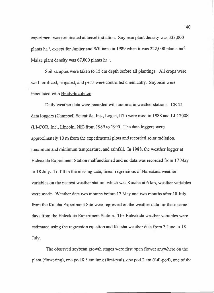
experiment was terminated at tassel initiation. Soybean plant density was 333,000
plants ha‘‘, except for Jupiter and Williams in 1989 when it was 222,000 plants ha‘‘.
Maize plant density was 67,000 plants ha’*.
Soil samples were taken to 15 cm depth before all plantings. All crops were
well fertilized, irrigated, and pests were controlled chemically. Soybean were
inoculated with Bradvrhizobium.
Daily weather data were recorded with automatic weather stations. CR 21
data loggers (Campbell Scientific, Inc., Logan, UT) were used in 1988 and LI-1200S
(LI-COR, Inc., Lincoln, NE) from 1989 to 1990. The data loggers were
approximately 1 0 m from the experimental plots and recorded solar radiation,
maximum and minimum temperature, and rainfall. In 1988, the weather logger at
Haleakala Experiment Station malfunctioned and no data was recorded from 17 May
to 18 July. To fill in the missing data, linear regressions of Haleakala weather
variables on the nearest weather station, which was Kuiaha at 6 km, weather variables
were made. Weather data two months before 17 May and two months after 18 July
from the Kuiaha Experiment Site were regressed on the weather data for these same
days from the Haleakala Experiment Station. The Haleakala weather variables were
estimated using the regression equation and Kuiaha weather data from 3 June to 18
July.
The observed soybean growth stages were first open flower anywhere on the
plant (flowering), one pod 0.5 cm long (first-pod), one pod 2 cm (flill-pod), one of the
40
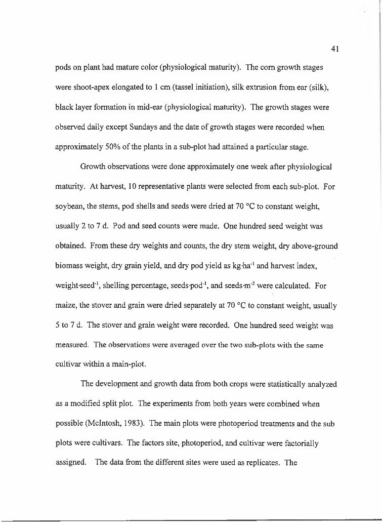
pods on plant had mature color (physiological maturity). The com growth stages
were shoot-apex elongated to 1 cm (tassel initiation), silk extrusion from ear (silk),
black layer formation in mid-ear (physiological maturity). The growth stages were
observed daily except Sundays and the date of growth stages were recorded when
approximately 50% of the plants in a sub-plot had attained a particular stage.
Growth observations were done approximately one week after physiological
maturity. At harvest, 10 representative plants were selected from each sub-plot. For
soybean, the stems, pod shells and seeds were dried at 70 °C to constant weight,
usually 2 to 7 d. Pod and seed counts were made. One hundred seed weight was
obtained. From these dry weights and counts, the dry stem weight, dry above-ground
biomass weight, dry grain yield, and dry pod yield as kg-ha*' and harvest index,
weight-seed'', shelling percentage, seeds-pod'', and seedsm'^ were calculated. For
maize, the stover and grain were dried separately at 70 °C to constant weight, usually
5 to 7 d. The stover and grain weight were recorded. One hundred seed weight was
measured. The observations were averaged over the two sub-plots with the same
cultivar within a main-plot.
The development and growth data from both crops were statistically analyzed
as a modified split plot. The experiments from both years were combined when
possible (McIntosh, 1983). The main plots were photoperiod treatments and the sub
plots were cuitivars. The factors site, photoperiod, and cultivar were factorially
assigned. The data from the different sites were used as replicates. The
41

experimental data was unbalanced because only control and natural photoperiod
treatments were planted in the winter 1988, the 1989 plantings among photoperiod
treatments were staggered, and in the longer photoperiod treatments some cultivars
did not flower. To correct for the imbalance, the winter 1988 and 1989 data, and the
non-flowering cultivars were not included in the analysis of variance for development
and growth of the crops. Then, one of these experimental designs was used for
analysis of variance: 1 ) randomized complete block with site as block and
photoperiod as treatment when data from only one year and one cultivar were
available, 2) combined year randomized complete block (McIntosh, 1983) with site as
block and photoperiod as treatment when data from two years and one cultivar were
available, 3) split-plot with site as replicate, photoperiod treatment as main plot, and
cultivar as sub plot when data from one year and more than one cultivar was
available, and 4) combined year split plot (McIntosh, 1983) with photoperiod
treatment as main plot and cultivar as sub plot when data from two years and more
than one cultivar were available. However, because the photoperiod treatments were
systematically assigned, the photoperiod source of variation cannot be tested for
significance (LeClerg et al., 1962).
Simulations of the field experiments were made using modified SOYGRO
v.5.42 and CERES-Maize v.2.1. The modification made on both models was to keep
photoperiod at a constant 14-, 17-, or 20-h when appropriate. In the models, the night
length or photoperiod values are functions of latitude and day of year. The variable
42

names that retain the nightlength or day length values are DURNIT in SOYGRO and
HRLT in CERES-Maize. To create constant photoperiod in the models, the variables
DURNIT and HRLT were set to the nightlength or daylength value corresponding to
the photoperiod treatment. The input parameters were set according to the soil
analysis results and management practices. The genetic coefficients were those
provided with the models (Tables 1 and 2; see definitions in Tables 7 and 8 ). With
CERES-Maize, the simulations were done with nitrogen balance subroutine
operating, but the water balance was not used because no water stress in the field was
assumed. With SOYGRO, the simulations were performed assuming no water stress.
The simulation results were compared with the results from the field.
Observed and simulated data were plotted for several growth and phonological
variables. Plots were made of simulated values on observed values. The data were
obtained specific to year, site, photoperiod treatment, and cultivar. A simple linear
regression was fitted through the data to estimate a trend. To estimate the trend, the
observed values were assumed to have little error so that linear regression may be
applied. Furthermore, the method of determining the structural relation between
observed and simulated data can affect the estimated slope and y-intercept. The
preferred method is reduced major axis. However, if the correlation coefficient (r)
between the observed and simulated results was greater than 0.7, the slope and y-
intercept would be similar whether ordinary least squares, reduced major axis, or
43
44
Table 1. Genetic coefficients of soybean cvs. 'Bragg', 'Evans', 'Jupiter', and 'Williams' for SOYGRO v.5.42.
Geneticcoefficient 'Bragg' 'Evans' 'Jupiter' 'Williams'
VARNl 5.0 5.0 5.0 5.0
VARNO 1 1 . 8 9.5 1 2 . 0 10.43
VARTH 13.5 2 . 0 18.62 6 . 0
VARDH 1 . 0 1 . 0 1 . 0 1 . 0
PHTHRS(l) 5.0 5.0 5.0 5.0
PHTHRS(2) 9.0 9.0 9.0 9.0
PHTHRS(3) 0 . 0 0 . 0 5.0 0 . 0
PHTHRS(4) 4.0 3.5 5.5 7.4
PHTHRS(5) 1 2 . 8 6 1 2 . 8 6 1 2 . 8 6 1 2 . 8 6
PHTHRS(6 ) 6.5 7.0 8.5 6 . 0
PHTHRS(7) 9.74 10.67 9.5 11.44
PHTHRS(8 ) 9.0 25.5 9.5 17.0
PHTHRS(9) 34.0 34.0 34.0 34.0
PHTHRS(IO) 47.5 44.0 42.0 43.0
PHTHRS(ll) 1 2 . 0 1 2 . 0 1 2 . 0 1 2 . 0
SHVAR 1 1 . 6 9.5 13.0 1 1 . 0
SDVAR 6 . 0 6 . 0 6 . 0 6 . 0
SDPDVR 2.05 2 . 2 2 . 1 2 . 2
PODVAR 2 0 0 . 0 160.0 2 0 0 . 0 1 2 0 . 0
FLWVAR 450.0 320.0 400.0 240.0
TRIFOL 0.33 0.38 0.34 0.35
SIZELF 171.4 173.47 173.7 188.37
SLAVAR 350.0 360.0 350.0 350.0
45
Table 2. Genetic coefficients of Pioneer hybrids 3475 and X304C for CERES- Maize v.2.1.
PI P2 P5 G2 G3Cultivar GDD' dh-‘ GDD' kernels plant’' mg-kernel’' -d’'
3475 2 0 0 0.70 800 725 8 . 6
X304C 320 0.52 980 625 6
' Growing degree days with base temperature 8 ° C.
some other fitting method was used (Flavelle, 1992). The means and standard
deviations for the observed and simulated variables were calculated (Little and Hill,
1978). Further statistical analyses were calculated according to equations by
Willmott (1981,1982). Mean square error (MSE), systematic mean square error
(MSE(s)), unsystematic mean square error (MSE(u)) were calculated.
MSE = /■I

46
MSE{u) = [ I ] • «-'/-I
where and were the simulated and observed values, P, bar equaled a + b ■ 0„ and n was the number o f observations.
The MSE(s) was partitioned into additive (MSE(a)) and proportional
(MSE(p)) components. These two components reflect the magnitude of the
systematic error as being additive or proportional. A third component,
interdependence (MSE(i)), was related to the correlation between MSE(a) and
MSE(p). The three components o f MSE(s) were calculated as,
MSE(a) =
MSE(p) = (6 - 1 )' • [«-' E O/]

47
MSE{i) = 2a • (6-1) • O
where a is the y-intercept of the fitted regression line, b is the slope of the line, and O is the mean of all observed values. The following relations hold for the mean square
errors,
MSE = MSE{s) + MSEiu)
MSE{s) = MSE{a) + MSE{p) + MSE{})
The mean absolute error (MAE) was calculated as,
MAE = \P-0,\ ] ■/-I
Lastly, the index of agreement {d) indicated the correspondence between the observed
and simulated values. Index o f agreement was calculated.
I [ \PrO)\ + \OrO\ V
The index of agreement varies from 0 to 1 where 0 signifies complete disagreement
between the observation and simulation and 1 means complete agreement.

A model that perfectly simulated the field experiments would produce a
linear regression with slope of 1 and y-intercept of 0 when simulated values were
regressed on observed. Any simulation that did not perfectly match the observed
value would change the regression line's slope, y-intercept, or increase error about the
regression line. The total deviation of simulation fi-om observation is mean square
error, MSE. The MSE can be partitioned into unsystematic error, MSE(u), and
systematic error, MSE(s) (Willmott, 1981; Willmott, 1982). Unsystematic error is
manifested in deviation about the regression line in a simulated vs. observed plot and
is a result of uncertainty in model parameters (Flavelle, 1992). Systematic error is
revealed in a slope other than 1 and/or y-intercept other than 0 (Willmott, 1981;
Willmott, 1982), that is, the deviation of the regression line from the expected line
with slope 1 and y-intercept 0. The systematic error results from a biased model or
biased input parameters (Flavelle, 1992). The systematic error can be further
partitioned into additive and proportional errors, MSE(a) and MSE(p) (Willmott,
1981). MSE(a) and MSE(p) quantify the deviations due to y-intercept and slope.
Because a change in slope can necessarily cause a change in y-intercept, the
deviations in slope and y-intercept can be interdependent. The interdependence error,
MSE(i), is the third partition in the systematic error. When MSE(i) becomes large,
MSE(a) and MSE(p) become meaningless, that is MSE(a) and MSE(p) are so greatly
interdependent that the systematic error cannot be readily attributed to additive or
proportional. While the systematic error can be partitioned into MSE(a), MSE(p),
48

and MSE(i), the relative magnitude of these deviations cannot identify the flaw in the
model or input parameters that caused the systematic error (Flavelle, 1992),
49
Results
Soybean cultivars displayed the expected sensitivity to photoperiod in the
field experiments. The analysis of variance indicated that cultivars 'Bragg' and
'Evans' had significantly different number of mainstem nodes (Table 3). Despite not
being allowed to test the significance of photoperiod on number of nodes, figure 1
indicated that node number increased with photoperiod. The increased number of
nodes indicated that vegetative development was prolonged at longer photoperiod.
The analysis of variance showed a significant cultivar-by-photoperiod interaction for
days to flowering (Table 3). Long photoperiod differently increased the days from
planting to flowering among the cultivars 'Bragg', 'Evans', and 'Williams' (Figure 2).
Orthogonal linear trend comparisons resolved the high latitude adapted cultivar
'Evans' had the smallest increase in days to maturity as photoperiod increased while
the low latitude adapted cultivar 'Bragg' had the greatest increase. Photoperiod had
intermediate effect on days to flowering for the mid-latitude adapted cultivar
'Williams'. In general low latitude adapted soybean are more photoperiod sensitive
than high latitude adapted plants, so artificial photoperiod extension was expected to
prolong soybean vegetative development.
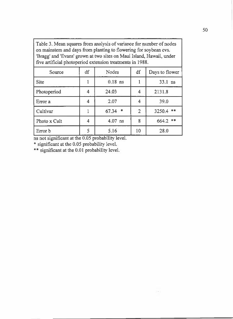
50
Table 3. Mean squares from analysis of variance for number of nodes on mainstem and days from planting to flowering for soybean cvs. 'Bragg' and 'Evans' grown at two sites on Maui Island, Hawaii, under five artificial photoperiod extension treatments in 1988.
Source df Nodes df Days to flower
Site 1 0.18 ns 1 33.1 ns
Photoperiod 4 24.03 4 2131.8
Error a 4 2.07 4 39.0
Cultivar 1 67.34 * 2 3250.4
Photo X Cult 4 4.07 ns 8 664.2 **
Error b 5 5.16 1 0 28.0ns not significant at the 0.05 probability level. * significant at the 0.05 probability level.** significant at the 0 . 0 1 probability level.
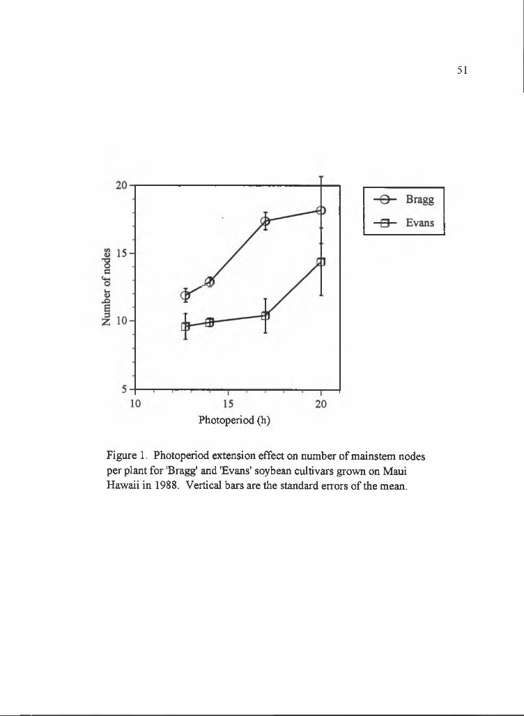
51
Photoperiod (h)
Figure 1. Photoperiod extension effect on number of mainstem nodes per plant for 'Bragg' and 'Evans' soybean cultivars grown on Maui Hawaii in 1988. Vertical bars are the standard errors of the mean.
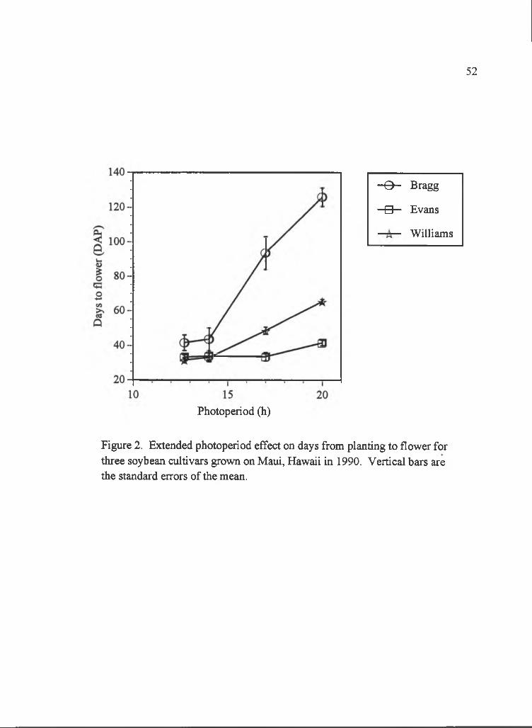
52
- e - Bragg
- a - Evans
Williams
Photoperiod (h)
Figure 2. Extended photoperiod effect on days from planting to flower for three soybean cultivars grown on Maui, Hawaii in 1990. Vertical bars are the standard errors of the mean.

Photoperiod effect on grain weight plant'* seemed related to the latitude that
cultivars were adapted. Analysis of variance did not indicate a significant
cultivar-by-photoperiod interaction for grain weight plant'* (Table 4), but orthogonal
linear trend comparison showed a significant (p>0.05) difference between 'Bragg' and
'Evans' over photoperiods. The plot of grain weight on photoperiod displayed the
greatest grain weight for the low latitude adapted cultivar 'Bragg' was at the shorter
photoperiod, while the greatest grain weight was at 2 0 h photoperiod for the high
latitude adapted cultivar 'Evans' (Figure 3). Grain weight plant'* seemed related more
to seed number plant'* than single seed weight. The seed number plant'* had
significantly different linear trends over photoperiods between the two cultivars
(p>0.05) and a plot of photoperiod effect on cultivar similar to grain weight plant'*
(Figure 4). The linear trend over photoperiods for single seed weight was
significantly different between the two soybean cultivars (p>0.05). Single seed
weight for 'Evans' was relatively constant across photoperiods, while 'Bragg' had
single seed weight that decreased as photoperiod increased (Figure 5). The closer
relation between grain weight plant'* and seed number plant'* suggested that yield was
more dependent on the number of seeds produced. The number of seeds plant'*
produced was greatest at the photoperiod the plants were supposingly adapted.
Maize hybrids were distinctly sensitive to photoperiod. The total number of
leaves, an indicator of the vegetative phase duration, had significant cultivar-by-
photoperiod interaction (Table 5). The leaf number increase with photoperiod was
53
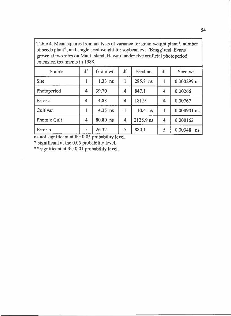
54
Table 4. Mean sqirares from analysis of variance for grain weight plant"', number o f seeds plant"', and single seed weight for soybean cvs. 'Bragg' and 'Evans' grown at two sites on Maui Island, Hawaii, under five artificial photoperiod extension treatments in 1988.
Source df Grain wt. df Seed no. df Seed wt.
Site 1 1.33 ns 1 285.8 ns 1 0.000299 ns
Photoperiod 4 39.70 4 847.1 4 0.00266
Error a 4 4.83 4 181.9 4 0.00767
Cultivar 1 4.35 ns 1 10.4 ns 1 0.000901 ns
Photo X Cult 4 80.80 ns 4 2128.9 ns 4 0.000162
Error b 5 26.32 5 880.1 5 0.00348 nsns not significant at the 0.05 probability level. * significant at the 0.05 probability level.** significant at the 0 . 0 1 probability level.
55
Photoperiod (h)
Figure 3. Photoperiod extension effect on grain dry weight per plant for 'Bragg' and 'Evans' soybean cultivars grown on Maui, Hawaii in 1988. Vertical bars are the standard errors of the mean.
56
- e - Bragg
- 0 - Evans
Photoperiod (h)
Figure 4. Photoperiod extension effect on seed number per plant for 'Bragg' and 'Evans' soybean cultivars grown on Maui, Hawaii in 1988. Vertical bars are standard errors of the mean.
57
0.25- e - Bragg
- a - Evans
15Photoperiod (h)
Figure 5. Photoperiod extension effect on single seed weight for 'Bragg' and 'Evans' soybean cultivars grown on Maui, Hawaii in 1988. Vertical bars are the standard errors of the mean.
58
Table 5. Mean squares from analysis of variance for total number of leaves plant'* for five maize hybrids grown at two sites on Maui Island, Hawaii, under five photoperiod treatments in 1990.
Source df Leaf number
Site 1 2.33 *
Photoperiod 4 25.11
Error a 4 0.31
Hybrid 4 108.73 **
Photo X Hybrid 16 3.51 **
Error b 2 0 0.51ns not significant at the 0.05 probability level. * significant at the 0.05 probability level.** significant at the 0 . 0 1 probability level.
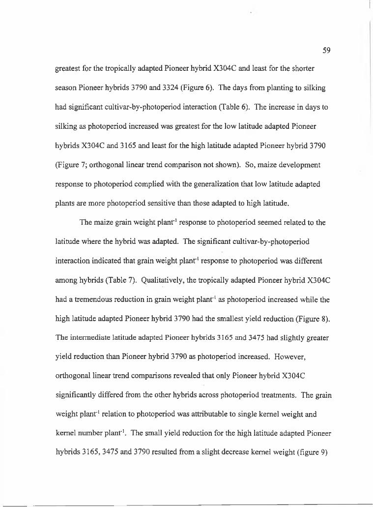
greatest for the tropically adapted Pioneer hybrid X304C and least for the shorter
season Pioneer hybrids 3790 and 3324 (Figure 6 ). The days from planting to silking
had significant cultivar-by-photoperiod interaction (Table 6 ). The increase in days to
silking as photoperiod increased was greatest for the low latitude adapted Pioneer
hybrids X304C and 3165 and least for the high latitude adapted Pioneer hybrid 3790
(Figure 7; orthogonal linear trend comparison not shown). So, maize development
response to photoperiod complied with the generalization that low latitude adapted
plants are more photoperiod sensitive than those adapted to high latitude.
The maize grain weight plant'' response to photoperiod seemed related to the
latitude where the hybrid was adapted. The significant cultivar-by-photoperiod
interaction indicated that grain weight plant ' response to photoperiod was different
among hybrids (Table 7). Qualitatively, the tropically adapted Pioneer hybrid X304C
had a tremendous reduction in grain weight plant ' as photoperiod increased while the
high latitude adapted Pioneer hybrid 3790 had the smallest yield reduction (Figure 8 ).
The intermediate latitude adapted Pioneer hybrids 3165 and 3475 had slightly greater
yield reduction than Pioneer hybrid 3790 as photoperiod increased. However,
orthogonal linear trend comparisons revealed that only Pioneer hybrid X304C
significantly differed from the other hybrids across photoperiod treatments. The grain
weight plant' relation to photoperiod was attributable to single kernel weight and
kernel number plant'. The small yield reduction for the high latitude adapted Pioneer
hybrids 3165, 3475 and 3790 resulted from a slight decrease kernel weight (figure 9)
59
60
10 15Photoperiod (h)
20
X304C
■O- 3165
- S - 3324
3475
- A - 3790
Figure 6 . Photoperiod extension effect on total leaf number per plant for Pioneer hybrids X304C, 3165, 3324, 3475, and 3790 grown on Maui, Hawaii in 1990. Bars are standard errors of mean.
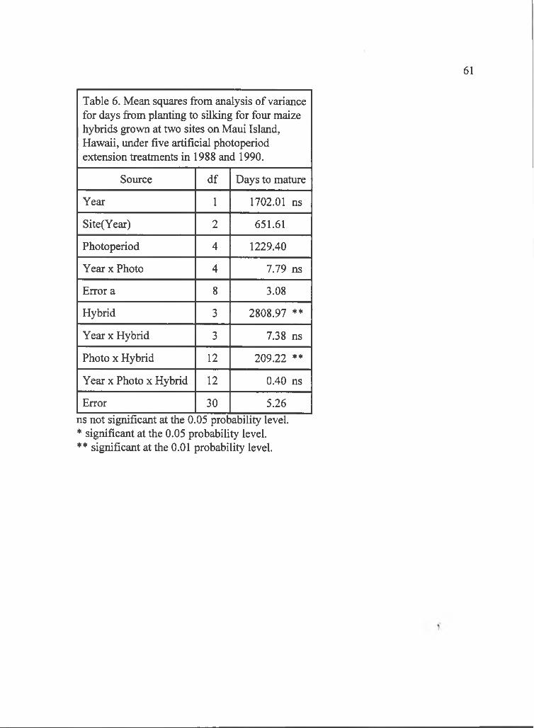
61
Table 6 . Mean squares from analysis of variance for days from planting to silking for four maize hybrids grown at two sites on Maui Island, Hawaii, under five artificial photoperiod extension treatments in 1988 and 1990.
Source df Days to mature
Year 1 1702.01 ns
Site(Year) 2 651.61
Photoperiod 4 1229.40
Year X Photo 4 7.79 ns
Error a 8 3.08
Hybrid 3 2808.97 **
Year X Hybrid 3 7.38 ns
Photo X Hybrid 1 2 209.22 **
Year X Photo x Hybrid 1 2 0.40 ns
Error 30 5.26ns not significant at the 0.05 probability level. * significant at the 0.05 probability level.** significant at the 0 . 0 1 probability level.
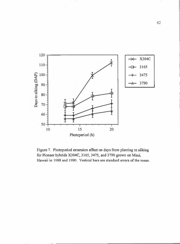
62
- X - X304C
- 0 - 3165
3475
- A - 3790
Photoperiod (h)
Figure 7. Photoperiod extension effect on days from planting to silking for Pioneer hybrids X304C, 3165, 3475, and 3790 grown on Maui, Hawaii in 1988 and 1990. Vertical bars are standard errors o f the mean.
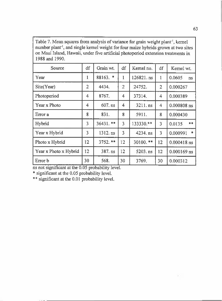
63
Table 7. Mean squares from analysis of variance for grain weight p lant', kernel number plant', and single kernel weight for four maize hybrids grown at two sites on Maui Island, Hawaii, under five artificial photoperiod extension treatments in 1988 and 1990.
Source df Grain wt. df Kernel no. df Kernel wt.
Year 1 88163. * 1 126821. ns 1 0.0605 ns
Site(Year) 2 4434. 2 24752. 2 0.000267
Photoperiod 4 8767. 4 37314. 4 0.000389
Year X Photo 4 607. ns 4 3211. ns 4 0.000808 ns
Error a 8 831. 8 5911. 8 0.000430
Hybrid 3 36431. ** 3 133330.** 3 0.0135 **
Year X Hybrid 3 1312. ns 3 4234. ns 3 0.000991 *
Photo X Hybrid 1 2 3752.** 1 2 30100. ** 1 2 0.000418 ns
Year X Photo x Hybrid 1 2 387. ns 1 2 5203. ns 1 2 0.000169 ns
Error b 30 568. 30 3769. 30 0.000312ns not significant at the 0.05 probability level. * significant at the 0.05 probability level.** significant at the 0 . 0 1 probability level.
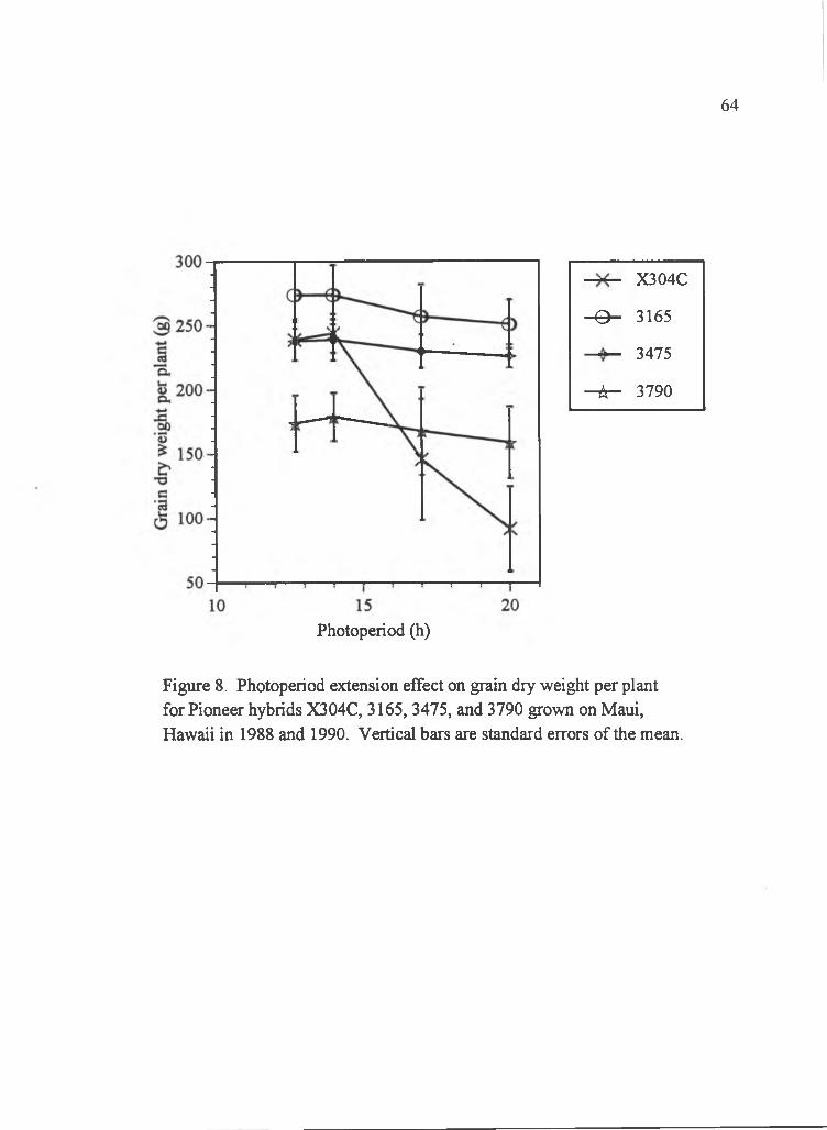
64
X304C
- 0 - 3165
3475
- A - 3790
Photoperiod (h)
Figure 8 . Photoperiod extension effect on grain dry weight per plant for Pioneer hybrids X304C, 3165, 3475, and 3790 grown on Maui, Hawaii in 1988 and 1990. Vertical bars are standard errors of the mean.
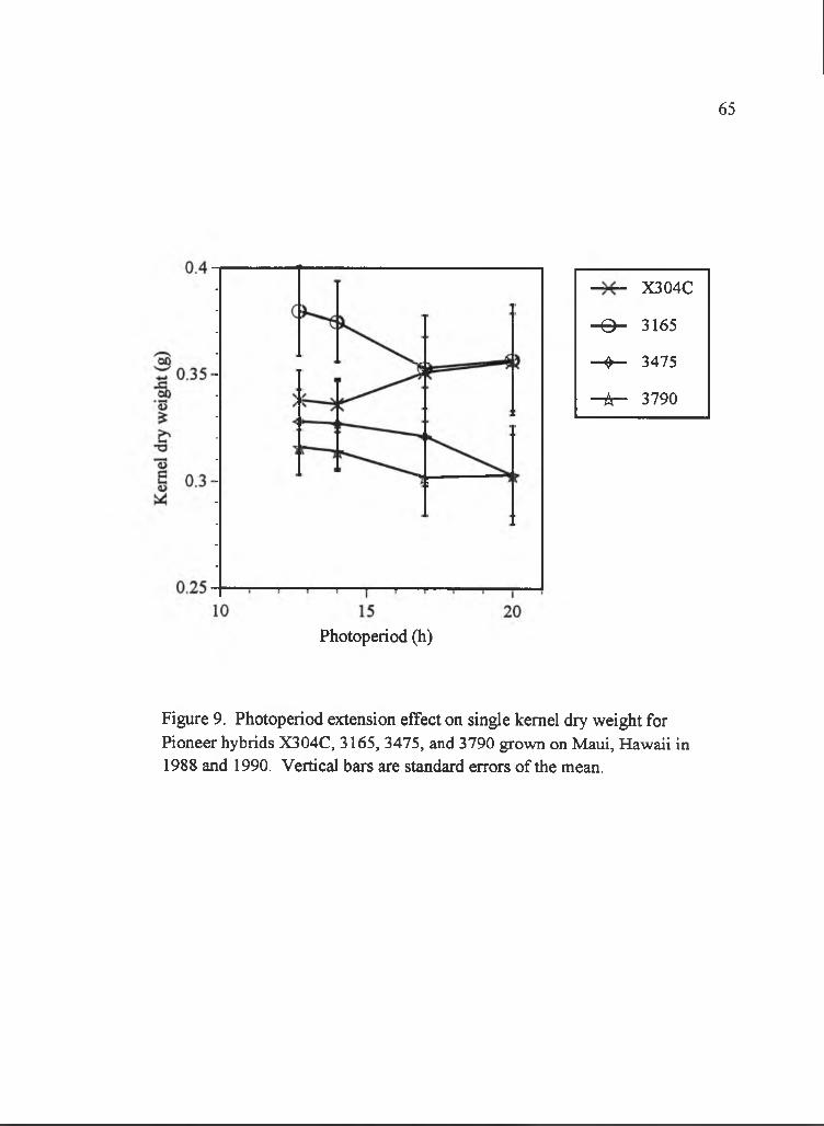
65
X304C
- 0 - 3165
0 — 3475
- i r - 3790
Photoperiod (h)
Figure 9. Photoperiod extension effect on single kernel dry weight for Pioneer hybrids X304C, 3165, 3475, and 3790 grown on Maui, Hawaii in 1988 and 1990. Vertical bars are standard errors of the mean.
rather than kernel number plant' which remained stable across photoperiod (figure
10). The yield components of the tropical adapted Pioneer hybrid X304C had a
unique response to photoperiod. The kernel number plant' greatly decreased as
photoperiod was increased from 14 to 20 h (Figure 9). The decrease in kernel number
for Pioneer hybrid X304C may be attributed to the increase in the tassel-silk interval
from 2.5 to 15 days as photoperiod increased from 12.7 to 20 h. Photoperiod
sensitivity of the tasseling-silking interval may be characteristic o f tropical adapted
genotypes (Bonhomme et al., 1994). The other hybrids had tassel-silk intervals 4 d or
less even at 20 h photoperiod. The increased interval for Pioneer hybrid X304C
could have resulted in few viable pollen falling on the silk, so fewer kernels were
produced (Manrique and Hodges, 1991). As a result of the few kernels produced, the
single kernel weight increased (Figure 10) presumably due to increased assimilate
supply (Schoper et al., 1982). So, the large yield reduction in Pioneer hybrid X304C
and only slight yield reduction in Pioneer 3790 as photoperiod increased
demonstrated that the high latitude adapted hybrids tolerated long photoperiods better
than the low latitude adapted hybrids.
The validation statistics (Willmott, 1981; Willmott, 1982) in tables 8 to 14
help to interpret the deviations of the simulated values from the observed values in
figures 11 to 25.
SOYGRO was able to simulate soybean development across wide ranges of
photoperiods and cultivars. The index of agreement (d) for days to flowering was
66
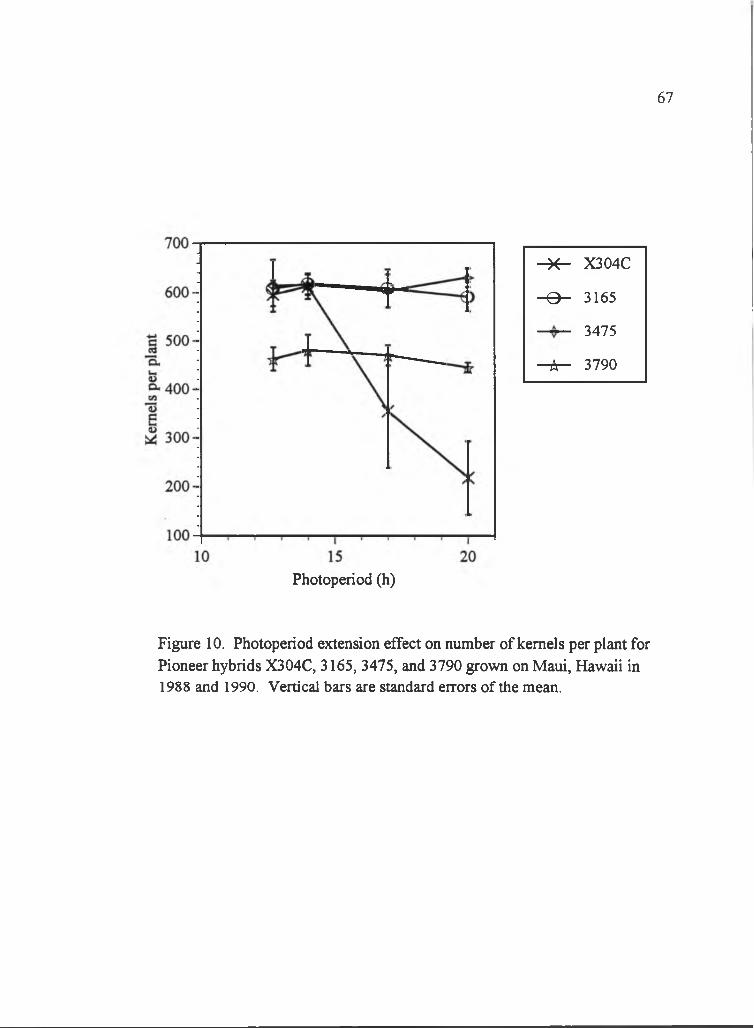
67
0 ^ X304C
- 0 - 3165
3475
-A - 3790
Photoperiod (h)
Figure 10. Photoperiod extension effect on number of kernels per plant for Pioneer hybrids X304C, 3165, 3475, and 3790 grown on Maui, Hawaii in 1988 and 1990. Vertical bars are standard errors of the mean.
relatively high and lower for full pod and physiological maturity (Table 8 ). The
observed vs. simulated plots (Figure 11 to 13) illustrate the relationships. The low
proportion of systematic error (MSE(s) • MSE"') in flowering, 19%, suggests that
improving the model or input parameter precision will not greatly improve the
simulation result. However, the higher proportion of unsystematic error in time to
full pod and maturity, 48% and 62% respectively, indicated that model or input
parameter bias correction can greatly improve the simulation of development for
these stages.
The very low d statistic for yield and the yield components weight-seed’' and
seed numberm’ (Table 9) indicates that these attributes were not well simulated
(Figures 14 to 16). Yield had a high proportion of systematic error, 82%, and only
18% unsystematic error. Partitioning the systematic error in yield revealed that
proportional error was much larger than additive error. The high proportional error
indicated that flaws within the model were multiplicative and should be corrected to
increase the slope of the observed vs. simulated plot. Weight-seed"' had mean square
error that was equally attributable to unsystematic and systematic error. The
systematic error was due to additive and proportional error. Improving the simulation
for weight-seed'* requires reducing the bias in the model or input parameters.
However, both yield and weight-seed"' had correlation coefficients lower than 0.7, so
the accuracy of this interpretation is questionable. Seed number m'^ had more
systematic than the unsystematic error, 60% versus 40%. The systematic error can be
68
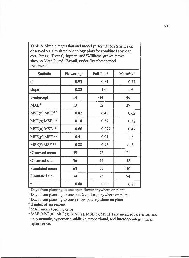
69
Table 8 . Simple regression and model performance statistics on observed vs. simulated phenology plots for combined soybean CVS. 'Bragg', 'Evans', 'Jupiter', and 'Williams' grown at two sites on Maui Island, Hawaii, vmder five photoperiod treatments.
Statistic Flowering' Full Pod^ Maturity'
d 0.93 0.81 0.77
slope 0.83 1 . 6 1 . 6
y-intercept 14 -14 -46
MAE' 13 32 39
M SE(u)M SE-'« 0.82 0.48 0.62
M SE(s)M SE-'" 0.18 0.52 0.38
MSE(a)MSE-'‘' 0 . 6 6 0.077 0.47
MSE(p)-MSE-'^ 0.41 0.91 1.5
MSE(i)M SE-'' 0 . 8 8 -0.46 -1.5
Observed mean 59 72 1 2 1
Observed s.d. 36 41 48
Simulated mean 63 99 150
Simulated s.d. 34 73 94
r 0 . 8 8 0 . 8 8 0.83
Days from planting to one pod 2 cm long anywhere on plant Days from planting to one yellow pod anywhere on plant d index of agreement
MAE mean absolute error® MSE, MSE(u), MSE(s), MSE(a), MSE(p), MSE(i) are mean square error, and
unsystematic, systematic, additive, proportional, and interdependence mean square error.
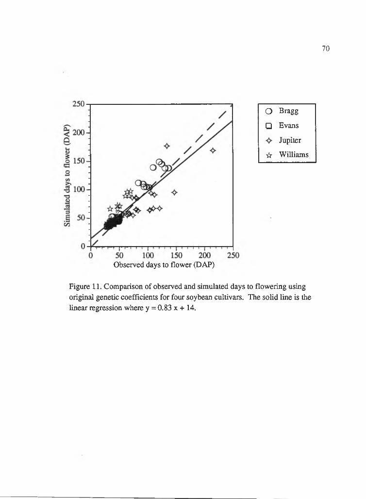
70
o Bragg
□ Evans
Jupiter
☆ Williams
Observed days to flower (DAP)
Figure 11. Comparison of observed and simulated days to flowering using original genetic coefficients for four soybean cultivars. The solid line is the linear regression where y = 0.83 x + 14.
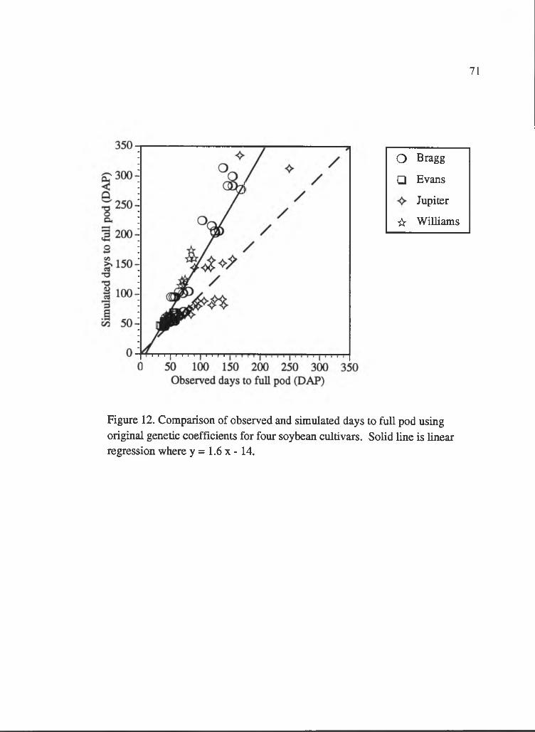
71
o Bragg
□ Evans
Jupiter
☆ Williams
Figure 12. Comparison of observed and simulated days to full pod using original genetic coefficients for four soybean cuitivars. Solid line is linear regression where y = 1.6 x - 14.
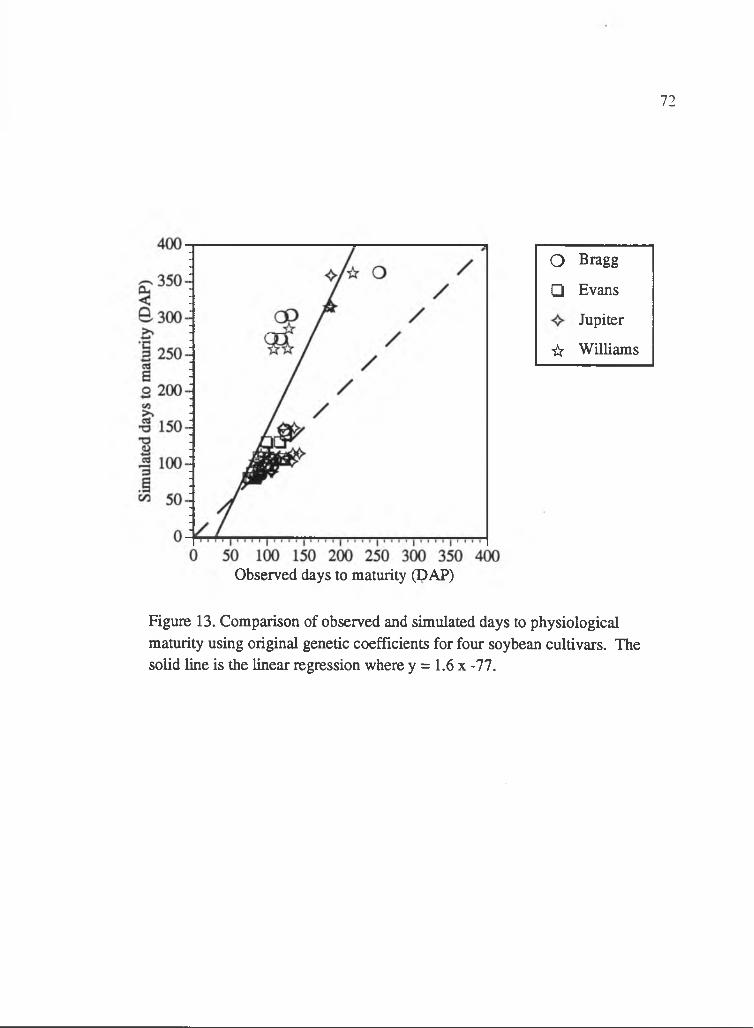
72
o Bragg
□ Evans
Jupiter
☆ Williams
Observed days to maturity (DAP)
Figure 13. Comparison of observed and simulated days to physiological maturity using original genetic coefficients for four soybean cultivars. The solid line is the linear regression where y = 1 . 6 x -7 7 .
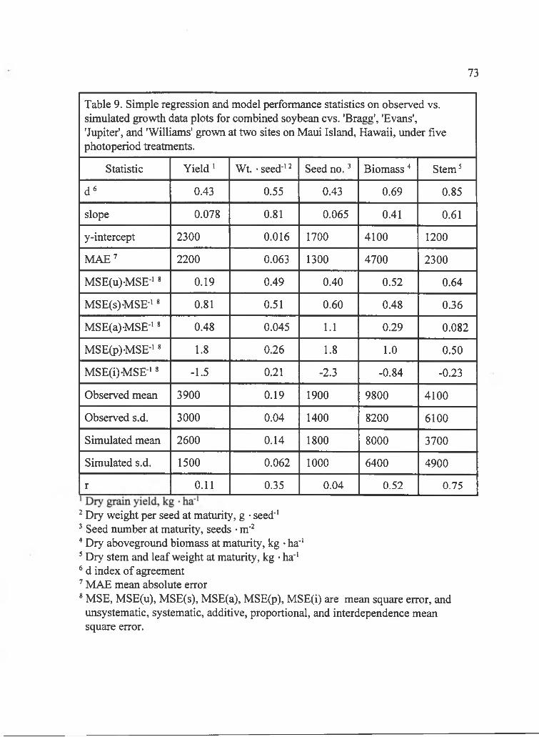
73
Table 9. Simple regression and model performance statistics on observed vs. simulated growth data plots for combined soybean cvs. 'Bragg', 'Evans', 'Jupiter', and 'Williams' grown at two sites on Maui Island, Hawaii, under five photoperiod treatments.
Statistic Y ield ' Wt. • seed"' ’ Seed no. ^ Biomass “ Stem^
d '' 0.43 0.55 0.43 0.69 0.85
slope 0.078 0.81 0.065 0.41 0.61
y-intercept 2300 0.016 1700 4100 1 2 0 0
M A E’ 2 2 0 0 0.063 1300 4700 2300
MSE(u)-MSE-'« 0.19 0.49 0.40 0.52 0.64
M SE(s)M SE-'« 0.81 0.51 0.60 0.48 0.36
MSE(a)-MSE-'» 0.48 0.045 1 . 1 0.29 0.082
MSE(p)-MSE-'« 1 . 8 0.26 1 . 8 1 . 0 0.50
MSE(i)-MSE-'« -1.5 0 . 2 1 -2.3 -0.84 -0.23
Observed mean 3900 0.19 1900 9800 4100
Observed s.d. 3000 0.04 1400 8200 6100
Simulated mean 2600 0.14 1800 8000 3700
Simulated s.d. 1500 0.062 1 0 0 0 6400 4900
r 0 . 1 1 0.35 0.04 0.52 0.75
Dry weight per seed at maturity, g • seed"' Seed number at maturity, seeds • m'^ Dry aboveground biomass at maturity, kg • ha"‘ Dry stem and leaf weight at maturity, kg • ha''
* d index of agreement’ MAE mean absolute error* MSE, MSE(u), MSE(s), MSE(a), MSE(p), MSE(i) are mean square error, and
unsystematic, systematic, additive, proportional, and interdependence mean square error.
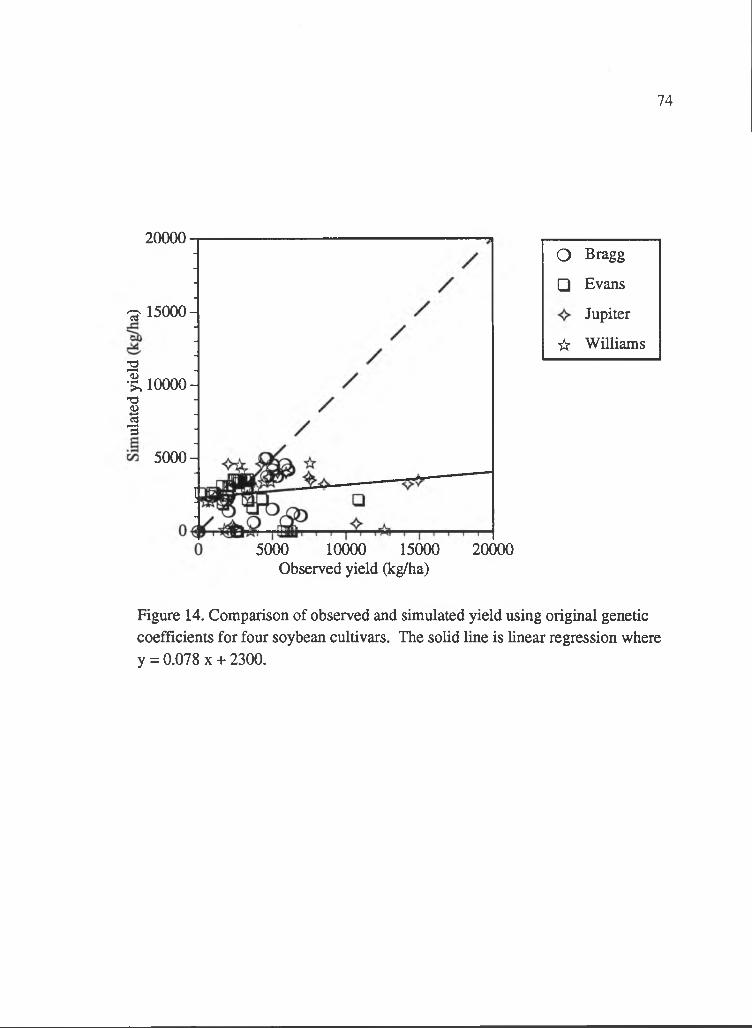
74
20000
a 15000-
2
1 . 10000-jT3
I35000-^
o Bragg
□ Evans
Jupiter
☆ Williams
5000 10000 15000Observed yield (kg/ha)
20000
Figure 14. Comparison of observed and simulated yield using original genetic coefficients for four soybean cultivars. The solid line is linear regression where y = 0.078 X + 2300.
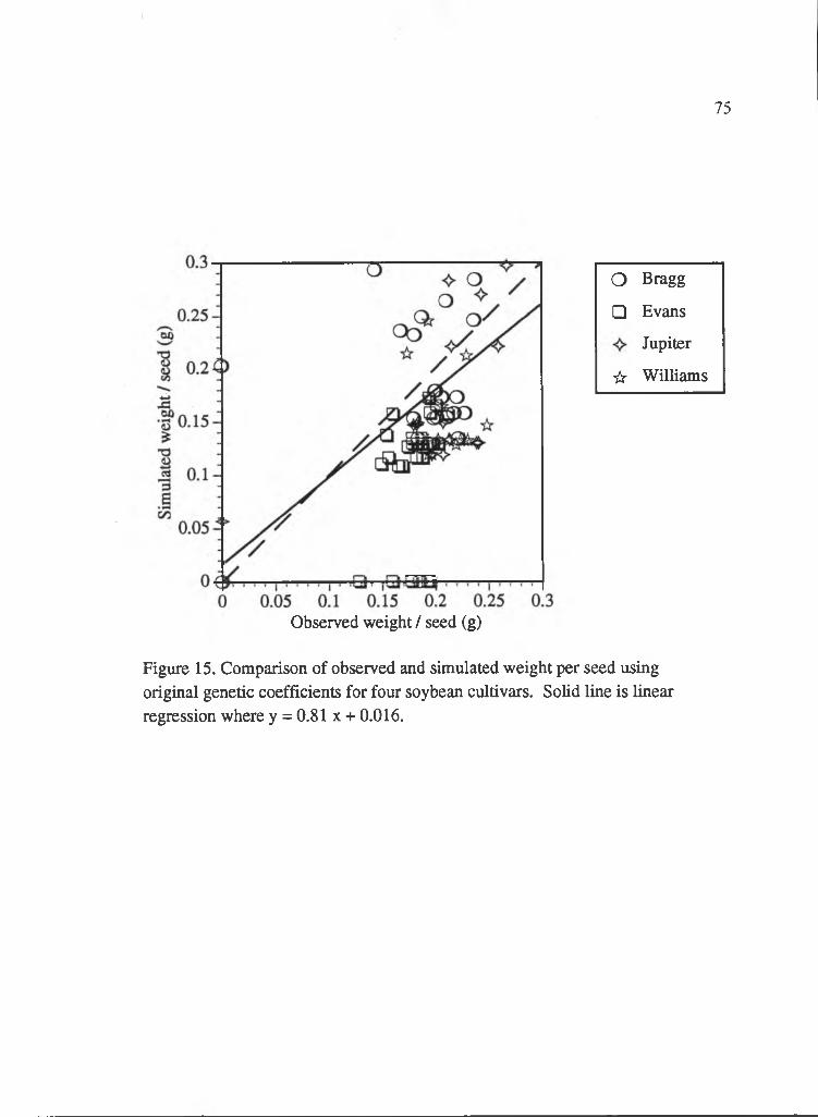
75
o Bragg
□ Evans
Jupiter
☆ Williams
Observed weight / seed (g)
Figure 15. Comparison of observed and simulated weight per seed using original genetic coefficients for four soybean cuitivars. Solid line is linear regression where y = 0.81 x + 0.016.
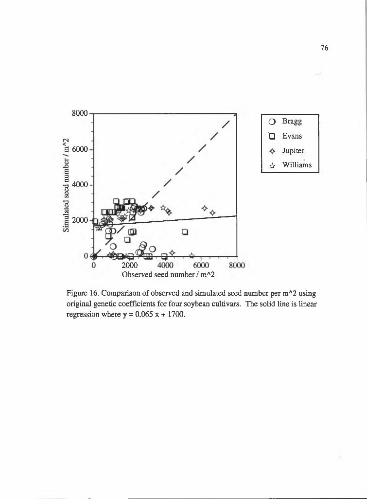
76
8000
cs 6 6000
Bsc'ST3
433
iz!
4000-
2000
o Bragg
□ Evans
Jupiter
☆ Williams
2000Observed seed number / m'^2
Figure 16. Comparison of observed and simulated seed number per m'^2 using original genetic coefficients for four soybean cultivars. The solid line is linear regression where y = 0.065 x + 1700.

partitioned, but the partitioned error would be difficult to interpret because of the high
interdependence error, MSE(i). Nevertheless, emphasis on correcting the model or
input parameter bias should improve the simulation of seed numberm'^.
The index of agreement for aboveground biomass at maturity was fairly low,
but higher for stem weight at maturity (Table 9) and was confirmed in the observed
vs. simulated plots (Figures 17 and 18). Biomass had mean square error evenly split
between systematic and unsystematic errors, but since the correlation coefficient was
below 0.7 the precision of the partitioned mean square error may be questionable.
The proportion of unsystematic mean square error was 64% for stem weight. So,
reducing input parameter bias or model correction should improve biomass and stem
weight simulation.
For CERES-Maize simulation of maize development, the low index of
agreement (d) for days to tassel initiation and high d for days to silking and
physiological maturity (Table 10) suggested that the simulations were inaccurate for
tassel initiation (Figure 19), but fairly accurate for silking and maturity (Figures 20
and 21). Tassel initiation had 64% of its mean square error as systematic, but again
the correlation coefficient was less than 0.7. Silking had high systematic error, and
high interdependence error that made interpretation of the partitioned systematic error
unreliable. Systematic and unsystematic errors were approximately equal for days to
maturity. The maturity interdependence was also very high. So, correcting model
77
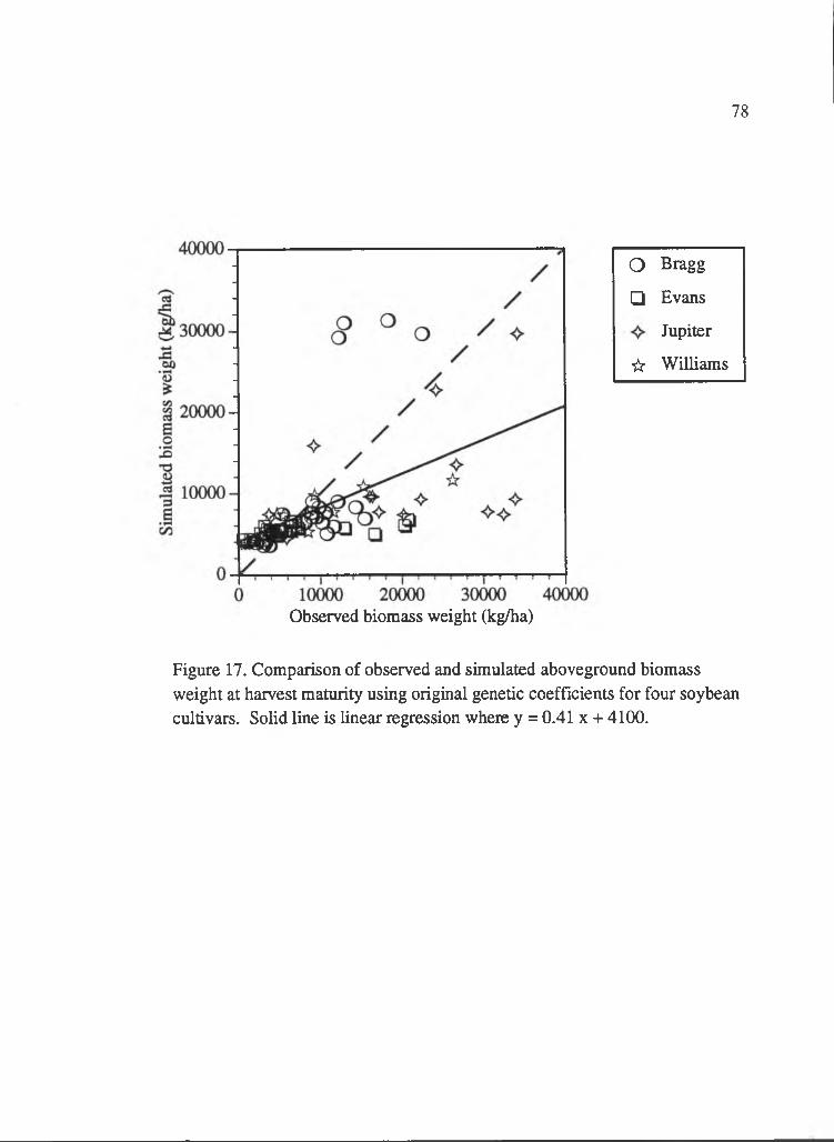
78
o Bragg
□ Evans
Jupiter
☆ Williams
Observed biomass weight (kg/ha)
Figure 17. Comparison of observed and simulated aboveground biomass weight at harvest maturity using original genetic coefficients for four soybean cultivars. Solid line is linear regression where y = 0.41 x + 4100.
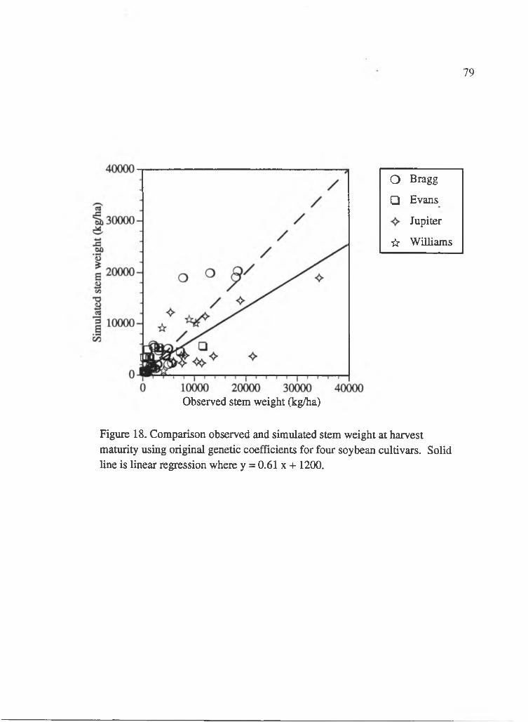
79
o Bragg
□ Evans
Jupiter
☆ Williams
Observed stem weight (kg/ha)
Figure 18. Comparison observed and simulated stem weight at harvest maturity using original genetic coefficients for four soybean cultivars. Solid line is linear regression where y = 0.61 x + 1 2 0 0 .
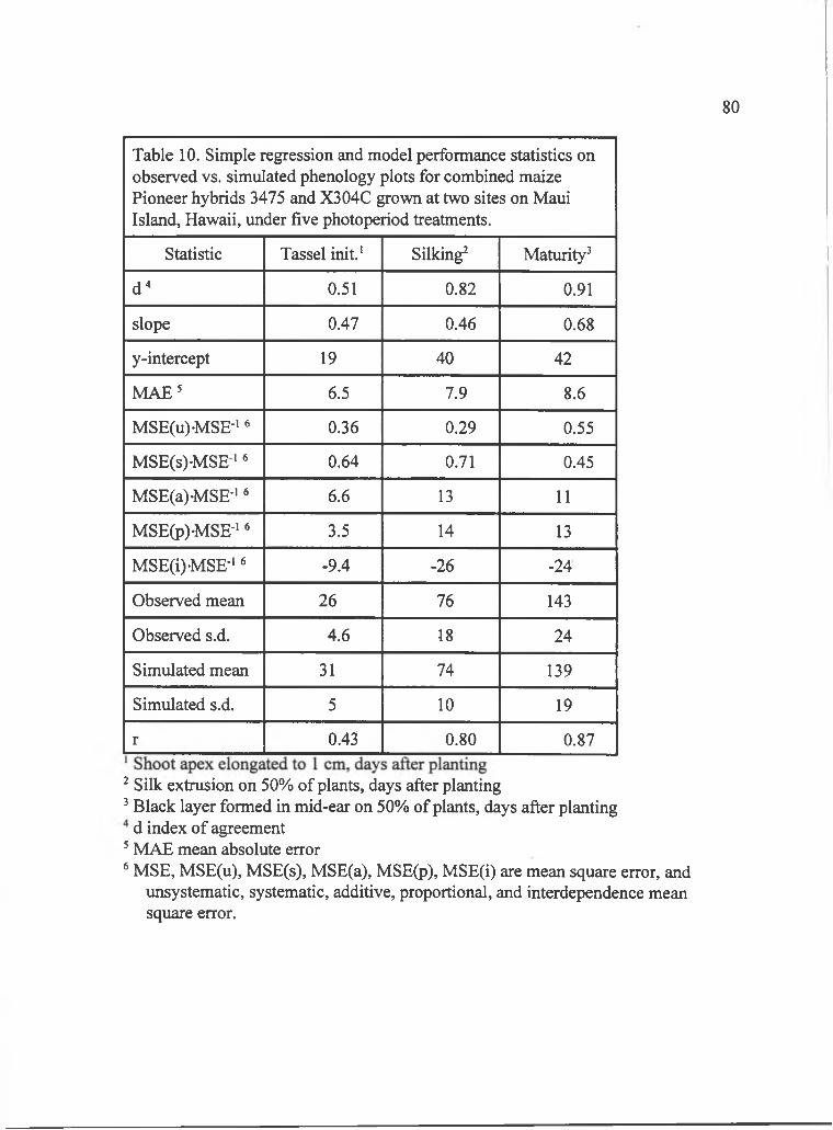
80
Table 10. Simple regression and model performance statistics on observed vs. simulated phenology plots for combined maize Pioneer hybrids 3475 and X304C grown at two sites on Maui Island, Hawaii, under five photoperiod treatments.
Statistic Tassel init.' Silking^ Maturity'
d" 0.51 0.82 0.91
slope 0.47 0.46 0 . 6 8
y-intercept 19 40 42
M A E ' 6.5 7.9 8 . 6
MSE(u)MSE-‘ ® 0.36 0.29 0.55
MSE(s)MSE * ® 0.64 0.71 0.45
M SE(a)M SE-'' 6 . 6 13 1 1
MSE(p)MSE-’ « 3.5 14 13
MSE(i)MSE-* ® -9.4 -26 -24
Observed mean 26 76 143
Observed s.d. 4.6 18 24
Simulated mean 31 74 139
Simulated s.d. 5 1 0 19
r 0.43 0.80 0.87
Silk extrusion on 50% of plants, days after planting Black layer formed in mid-ear on 50% of plants, days after planting d index of agreement
MAE mean absolute error® MSE, MSE(u), MSE(s), MSE(a), MSE(p), MSE(i) are mean square error, and
unsystematic, systematic, additive, proportional, and interdependence mean square error.
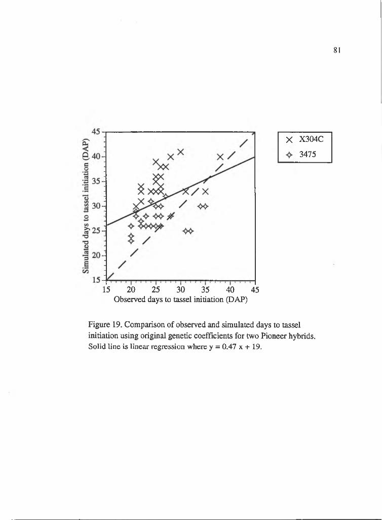
81
X X304C
3475
15 20 25 30 35 40 45Observed days to tassel initiation (DAP)
Figure 19, Comparison of observed and simulated days to tassel initiation using original genetic coefficients for two Pioneer hybrids. Solid line is linear regression where y = 0.47 x + 19.
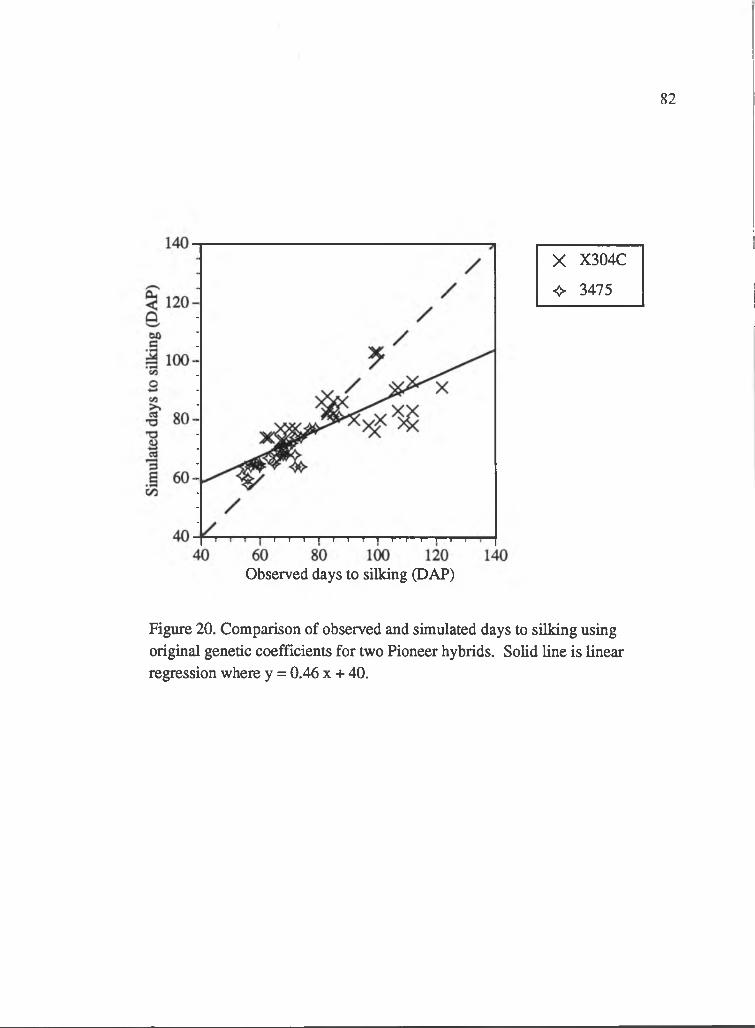
82
Observed days to silking (DAP)
X X304C
<> 3475
Figure 20. Comparison of observed and simulated days to silking using original genetic coefficients for two Pioneer hybrids. Solid line is linear regression where y = 0.46 x + 40.
83
X X304C
3475
Observed days to maturity (DAP)
Figure 21. Comparison of observed and simulated days to physiological maturity using original genetic coefficients for two Pioneer hybrids. Solid line is linear regression where y = 0.68 x + 42.
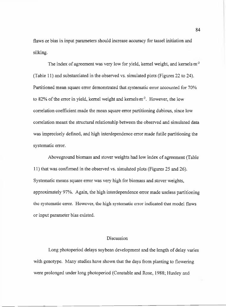
flaws or bias in input parameters should increase accuracy for tassel initiation and
silking.
The index of agreement was very low for yield, kernel weight, and kernels m '
(Table 11) and substantiated in the observed vs. simulated plots (Figures 22 to 24).
Partitioned mean square error demonstrated that systematic error accounted for 70%
to 82% of the error in yield, kernel weight and kernels-m"'. However, the low
correlation coefficient made the mean square error partitioning dubious, since low
correlation meant the structural relationship between the observed and simulated data
was imprecisely defined, and high interdependence error made futile partitioning the
systematic error.
Aboveground biomass and stover weights had low index of agreement (Table
11) that was confirmed in the observed vs. simulated plots (Figures 25 and 26).
Systematic means square error was very high for biomass and stover weights,
approximately 97%. Again, the high interdependence error made useless partitioning
the systematic error. However, the high systematic error indicated that model flaws
or input parameter bias existed.
Discussion
Long photoperiod delays soybean development and the length of delay varies
with genotype. Many studies have shown that the days from planting to flowering
were prolonged under long photoperiod (Constable and Rose, 1988; Huxley and
84
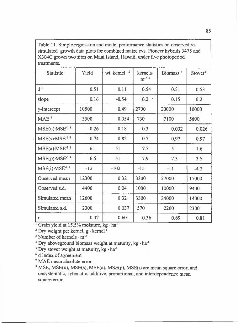
85
Table 11. Simple regression and model performance statistics on observed vs. simulated growth data plots for combined maize cvs. Pioneer hybrids 3475 and X304C grown two sites on Maui Island, Hawaii, under five photoperiod treatments.
Statistic Yield * wt. kernel'*’ kernels-m’“
Biomass '* Stover^
d^ 0.51 0 . 1 1 0.54 0.51 0.53
slope 0.16 -0.54 0 . 2 • 0.15 0 . 2
y-intercept 10500 0.49 2700 2 0 0 0 0 1 0 0 0 0
M A E’ 3500 0.054 730 7100 5600
MSE(u)-MSE’* * 0.26 0.18 0.3 0.032 0.026
MSE(s)MSE’*« 0.74 0.82 0.7 0.97 0.97
MSE(a)MSE’* * 6 . 1 51 7.7 5 1 . 6
MSE(p)-MSE'* * 6.5 51 7.9 7.3 3.5
MSE(i)MSE * * - 1 2 - 1 0 2 -15 - 1 1 -4.2
Observed mean 12300 0.32 3300 27000 17000
Observed s.d. 4400 0.04 1 0 0 0 1 0 0 0 0 9400
Simulated mean 12600 0.32 3300 24000 14000
Simulated s.d. 2300 0.037 570 2 2 0 0 2300
r 0.32 0.60 0.36 0.69 0.81Grain yield at 15.5% moisture, kg • ha‘
Dry weight per kernel, g • kernel’* Number of kernels • m’* Dry aboveground biomass weight at maturity, kg • ha * Dry stover weight at maturity, kg • ha'*
* d index of agreement’ MAE mean absolute error* MSE, MSE(u), MSE(s), MSE(a), MSE(p), MSE(i) are mean square error, and
unsystematic, sytematic, additive, proportional, and interdependence mean square error.
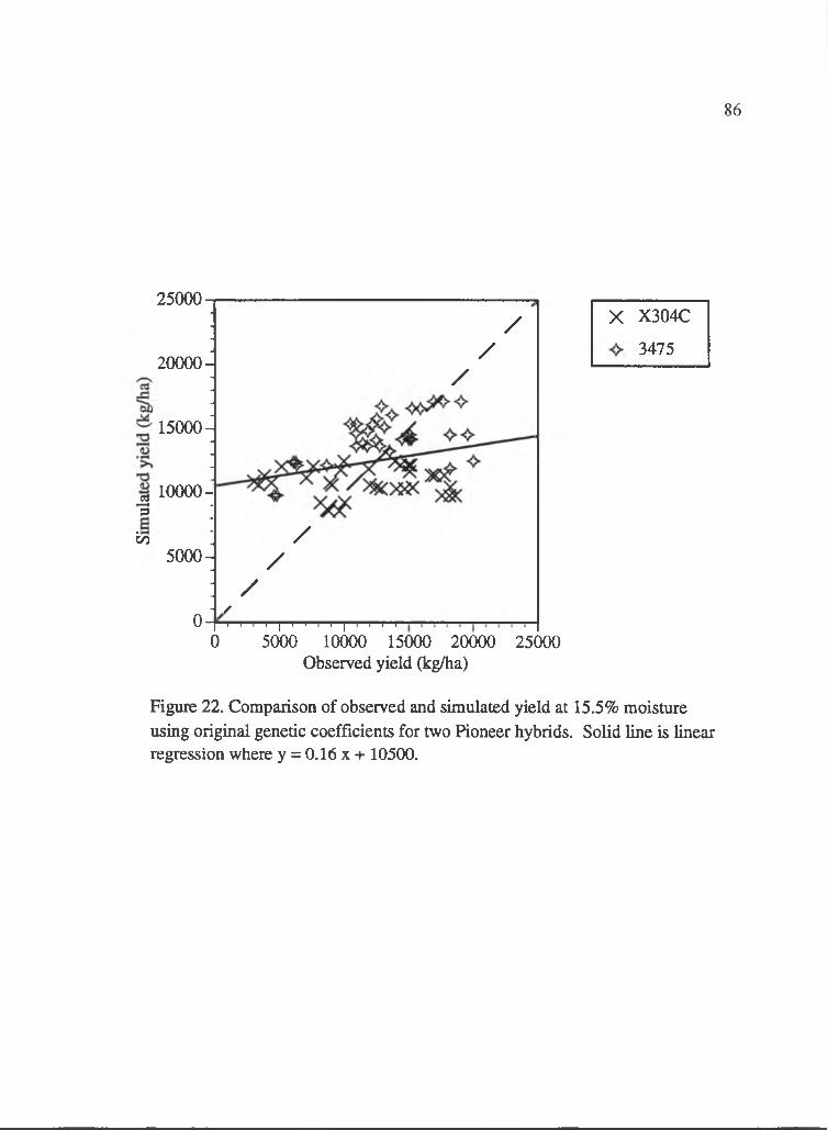
86
25000-
20000 -
15000-
23
i/3
10000-
5000-
//
/
/
0 -
0
///
I I I I I I I I I I I I I I
5000 10000 15000 20000Observed yield O^g/ha)
X X304C
3475
25000
Figure 22. Comparison of observed and simulated yield at 15.5% moisture using original genetic coefficients for two Pioneer hybrids. Solid line is linear regression where y = 0.16 x + 10500.
87
X X304C
3475
Observed kernel weight (g)
Figure 23. Comparison of observed and simulated kernel weight using original genetic coefficients for two Pioneer hybrids. Solid line is linear regression where y = -0.54 x + 0.49.
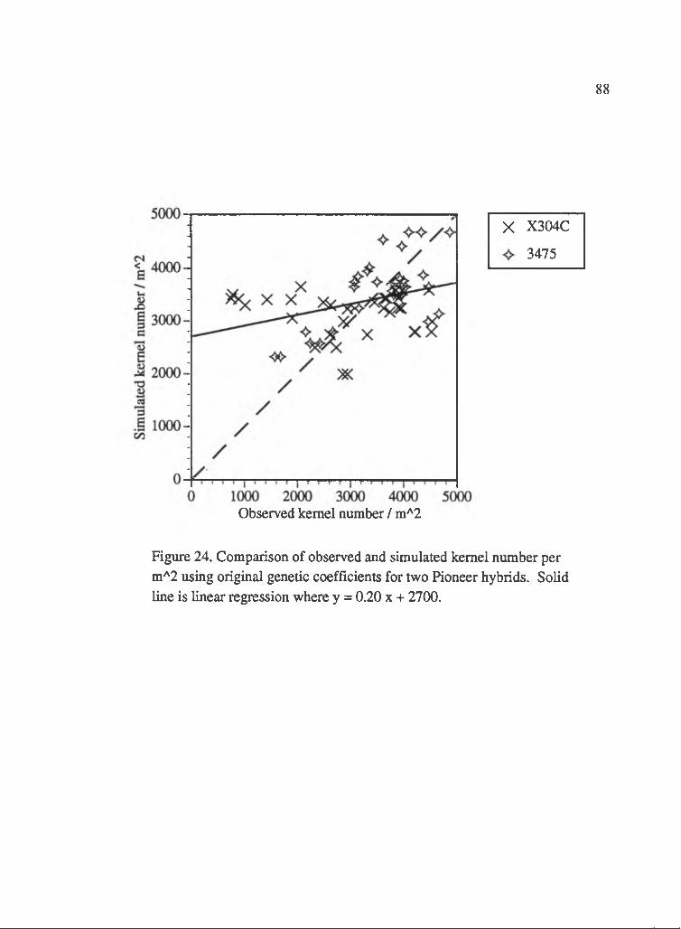
88
X X304C
3475
Observed kernel number / m'^2
Figure 24. Comparison of observed and simulated kernel number per m^ 2 using original genetic coefficients for two Pioneer hybrids. Solid line is linear regression where y = 0.20 x + 2700.
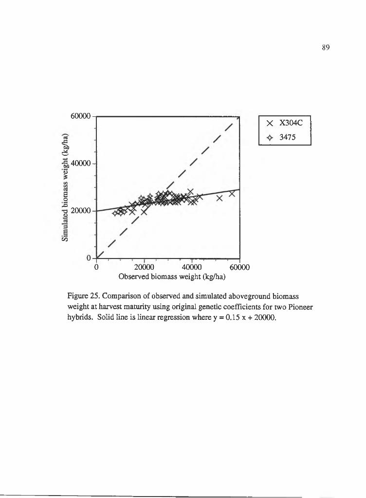
89
60000
ea
I-Sj 40000-]
%Boja
20000
e/3
X X304C
3475
0 20000 40000 60000Observed biomass weight (kg/ha)
Figure 25. Comparison of observed and simulated aboveground biomass weight at harvest maturity using original genetic coefficients for two Pioneer hybrids. Solid line is linear regression where y = 0.15 x + 20000.
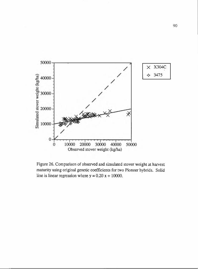
90
X X304C
<0> 3475
Observed stover weight (kg/ha)
Figure 26. Comparison of observed and simulated stover weight at harvest maturity using original genetic coefficients for two Pioneer hybrids. Solid line is linear regression where y = 0.20 x + 10000.

Summerfield, 1974; Summerfield et al., 1993). The magnitude of the delay to
flowering was generally greater for cultivars adapted to low latitude than cultivars
adapted to high latitude (Cregan and Hartwig, 1984; Major et al., 1975). The high
latitude adapted cultivars were presumed to be photoperiod insensitive, or had a very
high photoperiod threshold that prevented any delaying effect (Cregan and Hartwig,
1984). Hence, soybean development delay was greater for low latitude adapted
cultivars under long photoperiod (Parvez and Gardner, 1987).
Soybean cultivar differences in yield and yield components showed adaptation
to latitude or photoperiod. Soybean cultivars 'Clark' and 'Midwest', grown in Indiana,
had greater number of pods plant"' when grown under 16 h photoperiod than 12 or 20
h (van Schaik and Probst, 1958). Presumably, the two cultivars produced the most
pods in the photoperiod that was usual for Indiana. Similarly, soybean cultivars
adapted to lower latitude, maturity group VIII, produced the greatest number of pods
when grown at normal planting date in Florida (Parvez and Gardner, 1987).
However, pod number decreased 34 to 95% when photoperiod was shortened to 10 h
by covering plants with opaque plastic sheets or lengthened by planting at a later date.
Yield among cultivars from maturity groups II to IV grown in Illinois showed that the
early maturing cultivars do not tolerate short photoperiod (Schweitzer and Harper,
1985). Photoperiod was shortened to 10 h by covering plants with opaque plastic
sheets. The shortened photoperiod significantly reduced the yield for cultivars in
maturity group II, but did not significantly affect yield among the later maturing
91
cultivars. Furthermore, the soybean cultivar 'Ransom', maturity group VII, had
significantly reduced yield, pods planf', and single seed weight when grown in long
than short photoperiod (Raper and Thomas, 1978). So, similar to the results from the
field experiments with artificial photoperiod extension, soybean seems to produce
greater yield under photoperiod normally encountered at the latitude of adaptation.
Long photoperiod prolongs maize development. The time from planting to
tassel initiation was lengthened, with concomitant increase in total leaf number, when
maize was grown under long versus short photoperiod (Coligado and Brown, 1975;
Hunter et al., 1974; Warrington and Kanemasu, 1983c). Generally, tropical adapted
genotypes were more photoperiod sensitive than the temperate adapted in total leaf
number and time to tassel initiation (Warrington and Kanemasu, 1983c; Francis et al.,
1970). Photoperiod had no direct effect on the period from tassel initiation to silking
(Breuer et al., 1976; Warrington and Kanemasu, 1983a). Photoperiod affected the
phase from silking to physiological maturity, but the effect depended on temperature
(Breuer et al., 1976; Hunter et al., 1977). At 30 °C, silking to physiological maturity
duration decreased from 42 to 36 days when photoperiod was increased from 10 to 20
h. However, at 20 °C, silking to physiological maturity increased from 51 to 64 days
when photoperiod increased from 10 to 20 h (Breuer et al., 1976). So, the
photoperiod effect on prolonging maize development is mainly during the pre-tassel
initiation phase and, depending on temperature, the silking to physiological maturity
phase.
92
Photoperiod affects yield and yield components in temperate and tropical
hybrids. Twenty h versus 10 h photoperiod increased grain yield when a temperate
maize hybrid adapted to Ontario was grown at 20 °C in a growth chamber, but had no
effect at 30 °C (Hunter et al., 1977). At 20 °C, both single kernel weight and kernel
number plant"' increased under long photoperiod. Conversely, in a field trial,
photoperiod extended to over 18 h decreased yield of a temperate hybrid adapted to
Kentucky (Ragland et al., 1966). The yield decline was mainly attributed to
decreased single kernel weight in an April planting and decreased kernel number
plant"' in a June planting. Photoperiod extension of 15 h in the field reduced the yield
of a tropical maize hybrid (McClelland, 1928). The low yield was assumed to be a
result o f decreased kernel number plant"' caused by desychronization of tasseling and
silking (Ragland et al., 1966). For temperate and tropical maize hybrids, non-optimal
photoperiod reduced yield through decreased kernel number plant"' or single kernel
weight. Thus, these studies indicate that maize hybrid yield is greatest at its
photoperiod of adaptation.
SOYGRO generally simulated soybean development well, but improvements
in simulating days to maturity are possible. The error analysis statistics suggest that
errors in full pod and maturity simulation are due to model or input parameter error.
So, work is needed to correct the model or reduce the bias in input parameters that
affect days to maturity. Input parameters that affect days to maturity include the
genetic coefficients for photoperiod sensitivity and the post-flowering phase
93

durations. Bias in the genetic coefficients can be reduced by re-determining the
values through experiment or a calibration-type process.
The error in simulated soybean grain yield and aboveground biomass seems to
be related to the error in seed numberm'^. The simulated yield is dependent on the
yield components weight-seed* and seed number-m'^. Any error in the yield
components will be reflected in the yield unless the errors are offsetting.
Furthermore, any error in yield or stem weight will be reflected in aboveground
biomass because the aboveground biomass is the sum of grain yield and stem weight.
The dependence of yield on seed number and the dependence of biomass on yield
implies that improving the accuracy of seed number would improve the accuracy of
yield and biomass. The error analysis in the present experiment showed that seed
number deviation was attributed mainly to model or input parameter bias. So,
concentrating effort primarily on correcting the model or input parameter bias in seed
number should ameliorate simulation of yield and biomass.
CERES-Maize was able to simulate maize development well for days to
silking and maturity, but not for tassel initiation. Error in simulated tassel initiation
was mostly systematic. So, to improve the simulated com development, model or
input parameter correction is needed. Input parameters that may be corrected include
the genetic coefficients that control photoperiod sensitivity and the juvenile phase
duration.
94

Changes in CERES-Maize may be needed to correct the simulated growth
attributes yield and aboveground biomass. The yield components kernel weight and
kernels-m"' had very high systematic errors that require model or input parameter
change to correct. Then with the yield components corrected, improvement in yield
simulations would result. Stover weight also had large systematic error indicating the
necessity to change the model or input parameters. Changes in the model or input
parameters to correct the stover weight, with concomitant changes to correct yield,
would improve simulated aboveground biomass because aboveground biomass is the
sum of grain yield and stover weight.
The problem that caused the inaccurate simulation of stover weight in
CERES-Maize may be related to leaf area. One possibility to account for the
incorrect stover simulation may be the total carbohydrate production. Carbohydrate
production in CERES-Maize is a fimction of leaf area, solar radiation, water stress,
temperature, and soil nitrogen (Jones and Kiniry, 1986). In the simulations, no water
stress was assumed across photoperiod treatments, locations, and years. While solar
radiation, temperature, and soil nitrogen changed over time and space, the effects
were not likely to be large enough to accovmt for the large differences between the
observed and simidated stover weights. CERES-Maize calculates leaf area as a
fimction of leaf number-plant'' and area-leaf' (Jones and Kiniry, 1986). In turn, leaf
number is a fimction of leaf initiation rate, assumed constant, and thermal time from
sowing to tassel initiation. Hence, any bias in simulating time to tassel initiation will
95
result in bias in leaf area and, ultimately, stover weight. Also, area-leaf' may increase
with increasing photoperiod (Manrique and Hodges, 1991), but this is not simulated
in CERES-Maize. So, the inaccurate stover weight may be a result of the
imprecision in days to tassel initiation and area-leaf.
SOYGRO and CERES-Maize, with the present set of genetic coefficients and
for the varieties tested, were able to simulate development, but not growth. The
problems with simulating growth may not be in the genetic coefficients, but in the
model itself
Modification to SOYGRO may be required to correct growth. The growth
attributes, especially weight-seed"' and seed number-m‘ , require both change in input
parameters and the model to improve the simulation of yield and biomass. The
possible inputs to change include the genetic coefficients, soil properties, soil initial
conditions, weather variables, and crop parameters. The changes in the input
parameters should be tried first to determine whether change in the model is
absolutely necessary to improve the growth simulation.
CERES-Maize simulated maize development fairly well, but growth was not.
Days to silking and maturity were fairly well simulated across the various
photoperiods, years, sites, and cultivars. However, tassel initiation was not well
simulated and the model may need changing to correct the problem. The growth
attribute kernel weight obviously needs change because the observed vs. simulated
plot has negative slope. Kernels-m'^ was not well simulated because the model over
96

estimated the number of kernels for Pioneer hybrid X304C. Manrique and Hodges
(1991) noted that in very long photoperiod, Pioneer hybrid X304C had fewer kernels
per ear due to de-synchronization of pollen-shed and silking. The model does not
have the ability to simulate kernel number in very long photoperiod for the tropically
adapted variety Pioneer hybrid X304C. With the poor simulation of kernel weight
and kernels m '’, yield was not accurately simulated. Further work may be needed to
improve the total carbohydrate production for better stover and biomass simulation.
The improvements may include changes in the calculation of leaf number and
area-leaf*.
97

CHAPTER 3
EVALUATING METHODS TO ESTIMATE GENETIC COEFFICIENTS IN
SOYGRO AND CERES-MAIZE
Introduction
Crop models contain genetic coefficients that quantify the genotype effects on
development and grovrih. Genetic coefficients describe either the development rate
response to environmental factors such as temperature and photoperiod, or potential
growth rates and quantities. The development and growth genetic coefficients for
SOYGRO and CERES-Maize are listed in tables 12 and 13 (Jones et al., 1986; Jones
and Kiniry, 1986). The crop models assume temperature and photoperiod are the
major environmental factors that affect development. Hence, the duration from stage
to stage is based on thermal time concept and photoperiod sensitivity. The growth
genetic coefficients define the genetic potential for characteristics such as yield
components, growth rates, and leaf area. These genetic potentials are modified within
the model through estimated water, temperature, nitrogen, or reduced photosynthate
stresses. Therefore, the genetic coefficients are critical in simulating crop response to
its environment.
There are two approaches to estimating genetic coefficients. One approach is
to incrementally change the genetic coefficients until the simulation and observed
crop characteristics match (Jones et al., 1989; Ritchie et al., 1992). This fitting
98

99
Table 12. Developmental and growth genetic coefficients in SOYGRO.
Genetic coefficient name Description
VARNl A threshold for night length that sets the night time accumulator at the minimum rate when night length is less than this value, in h.
VARNO A threshold for night length that sets the night time accumulator at the maximum rate when night length is greater than this value, in h.
VARTH Number of nights needed to accrue one unit of night time accumulator when night length is less than VARNl, the minimum development rate.
VARDH Number of nights needed to accrue one unit o f night time accumulator when night length is greater than VARNO, the maximum development rate set at 1.
PHTHRS (1) Physiological days from planting to emergence.
PHTHRS (2) Physiological days from emergence to unifoliolate stage.
PHTHRS (3) Physiological days from unifoliolate to end of juvenile stage.
PHTHRS (4) Units of night time accumulator from end of juvenile stage to floral induction.
PHTHRS (5) Number of physiological days from floral induction to flowering.
PHTHRS (6) Units of night time accumulator from flowering to beginning pod stage.
PHTHRS (7) Units of night time accumulator from flowering to full pod stage.
PHTHRS (8) Units of night time accumulator from flowering to expanded last leaf
PHTHRS (9) Night time accumulator units from flowering to last flower.
PHTHRS (10) Night time accumulator imits from flowering to physiological maturity.
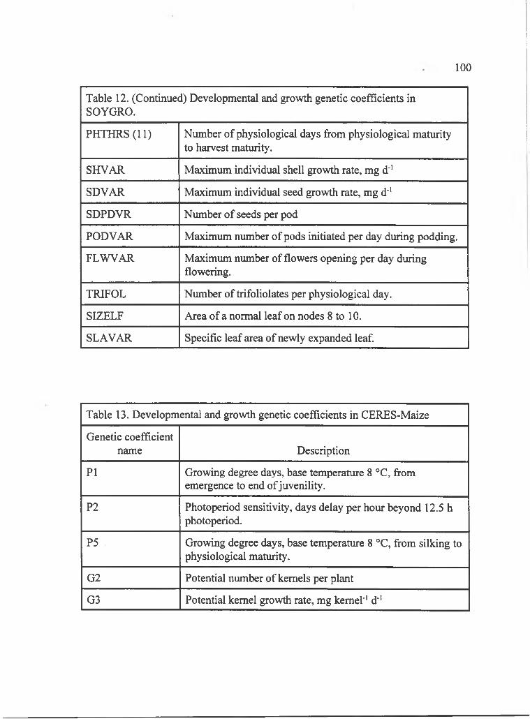
100
Table 12. (Continued) Developmental and growth genetic coefficients in SOYGRO.
PH T H R S(ll) Number of physiological days from physiological maturity to harvest maturity.
SHVAR Maximum individual shell growth rate, mg d"'
SDVAR Maximum individual seed growth rate, mg d'*
SDPDVR Number of seeds per pod
PODVAR Maximum number of pods initiated per day during podding.
FLWVAR Maximum number of flowers opening per day during flowering.
TRIFOL Number of trifoliolates per physiological day.
SIZELF Area of a normal leaf on nodes 8 to 10.
SLAVAR Specific leaf area of newly expanded leaf.
Table 13. Developmental and growth genetic coefficients in CERES-Maize
Genetic coefficient name Description
PI Growing degree days, base temperature 8 °C, from emergence to end of juvenility.
P2 Photoperiod sensitivity, days delay per hoin beyond 12.5 h photoperiod.
P5 Growing degree days, base temperature 8 °C, from silking to physiological maturity.
G2 Potential number of kernels per plant
G3 Potential kernel growth rate, mg kernel"' d"'

method has been lised to successfully simulate maize production in diverse climates
as South Africa, Mid-west U.S., and Brazil (du Pisani, 1987; Hodges et al., 1987; Liu
et al., 1989). The other approach requires detailed measurements of crop
development and growth in growth chamber or field experiments (Ritchie et al.,
1986).
The objective of this experiment is to determine the suitability of the two
methods for calculating genetic coefficients in SOYGRO and CERES-Maize. If the
models truly simulate the response of plant processes to the environment, the fitting
or experimental method to estimate genetic coefficients should be stable when
estimated across different environments. Stability of genetic coefficients estimated
across environments implies that the coefficients established in one environment can
be used to simulate crop growth and development in another environment.
Methods and Materials
The field experiments were described in the previous chapter, but the
procedures are briefly explained here. Identical experiments were conducted at two
sites on Maui Island, Hawaii. The site elevations were 640 m at Haleakala
Experiment Station (clayey, oxidic, isothermic Humoxic Tropohumult) and 282 m at
Kuiaha (clayey, ferritic, isohyperthermic Humoxic Tropohumult). The experimental
design was a split-plot where photoperiod was the main-plot and cultivar was the sub
plot. The natural photoperiod was extended with quartz lamps (minimum 4 W m’’ at
101

soil surface) to produce 20-, 17-, 14-, and natural + 0.5 h treatments. Natural
photoperiod was used as a control treatment. Four soybean cultivars ('Bragg', 'Evans',
'Jupiter', and 'Williams') and five maize hybrids (Pioneer hybrids X304C, 3165, 3324,
3475, and 3790) were planted in 1.5 by 3.0 m sub-plots. The plots were fertilized,
well irrigated, and pests were chemically controlled. These experiments were planted
four times over three years.
Data on weather, date of development stages, and growth characters were
observed. Daily maximum and minimum air temperature, rainfall, and solar radiation
were recorded on automatic weather stations (LI-1200S, LI-COR, Inc., Lincoln, NE).
Dates were observed when 50% of soybean plants within a plot reached the
development stages planting, emergence, unifoliolate, first flower, first 0.5 cm pod,
first 2 cm pod (full pod), last flower opened, last leaf fully expanded, and
physiological maturity. The area of a single leaf on the upper 5 nodes from 10 plants
and its dry weight was obtained between first flower and 2 cm pod growth stages. At
harvest maturity, the pod number, seed number, shell dry weight, seed dry weight,
stem dry weight, and number of nodes on the mainstem from 20 plants were
determined. Dates were recorded when com development stages were observed.
These stages were planting, emergence, apex elongated 1 cm (tassel initiation),
silking, and physiological maturity. Leaves 5 and 10 were marked with indelible ink
on 10 plants to obtain total leaf number. At harvest maturity, the grain and stover dry
weights, and kernel number were recorded. For each cultivar, each measurement was
1 0 2

made on two plots that were randomized within a photoperiod treatment. The mean
measurement for each cultivar within a photoperiod plot was lised to generate genetic
coefficients.
Two methods were used to estimate the genetic coefficients for SOYGRO and
CERES-Maize. The first method was to calculate genetic coefficients that describe
the rates of development and growth based on field observations of growth stages,
weights, and sizes. This method was considered as an explicit method. The second
method involved manipulating the genetic coefficient values until crop development
and growth fi-om the simulations matched those from the field experiments. This
method was called fitting.
An explicit method to determine the SOYGRO v.5.42 genetic coefficients was
not possible because the proper data were not collected. In the model, shell and seed
growth are dependent on the number of shells. Shell number, in turn, is dependent on
the number of flowers and pods produced per day during reproductive development.
The actual number o f flowers and pods produced per day during the flowering to
podding phase was not recorded. So, most of the growth genetic coefficients could
not be calculated. Most of the development genetic coefficients were related to
photoperiod or photothermal time. Estimating the photoperiod genetic coefficients
would be very similar to the fitting procedure and so was not done.
SOYGRO genetic coefficients were determined with a fitting method. Before
the fitting procedure was done, the model was modified. The night length variable
103
DURNIT was set to mimic the photoperiod treatments in the field. The genetic
coefficient PHTHRS(5), which was normally set to 12.86 (Jones et al., 1986), was
changed to 6.20 as derived from the data of Thomas and Raper (1983). The array
sizes for seed number, seed weight, shell number, shell weight, and flower number
were increased from 200 to 365. These changes were necessary to match simulation
results to the observations in the field experiments.
SOYGRO genetic coefficients were manipulated until simulated target data
were within 1% of the observed. PHTHRS(l) and PHTHRS(2) were changed until
simulated emergence and unifoliolate dates matched the observed dates. The juvenile
phase genetic coefficient PHTHRS(3) was set to 0.0 for cultivars 'Bragg', 'Evans', and
'Williams' and assumed 5.0 for 'Jupiter'. While VARDH was assumed to be 1.0, the
following was done to fit the photoperiod sensitivity genetic coefficients VARNO,
VARNl, and VARTH. Using only the control and natural photoperiod treatments
that had night length greater than 12 h (Jones et al., 1989), PHTHRS(4) was changed
until simulated flowering date matched the observed. The fitted PHTHRS(4) value
was used to simulate flowering date in the 14-, 17-, and 20-h photoperiod treatments.
VARNO and VARTH were modified until the simulated and observed flowering
dates for the 14- and 20-h treatments agreed. To fit the 17-h photoperiod treatment,
VARNO and VARNl were concurrently changed until simulated and observed
flowering dates matched. This fitting procedure was inadequate for 'Evans' because
VARNl was less than 4 h. So, VARNl was set to 0.0. After photoperiod sensitivity
104

was determined, PHTHRS(6), PHTHRS(7), PHTHRS(8), PHTHRS(9), and
PHTHRS(IO) were incrementally altered until the dates for first 0.5 cm pod, first 2
cm pod, last flower opened, last fully expanded leaf, and physiological maturity from
the simulation coincided with the observed. The growth genetic coefficient TRIFOL
was adjusted until the simulated number of nodes on the mainstem at harvest maturity
agreed with the observed. SIZELF and SLAVAR were calculated from the observed
leaf area and weight, and temperature (TPHFAC) and solar radiation (PARSLA)
correction in SOYGRO. The growth genetic coefficients for maximum pod addition
rate (PODVAR), maximum flower addition rate (FLWVAR), seeds per pod
(SDPDVR), maximum shell growth rate (SHVAR), maximum seed growth rate
(SDVAR), and photosynthetic correction (PHFAC3) were concurrently determined.
PODVAR was adjusted until simulated pod number plant'' at harvest maturity
matched the observed data. As PODVAR was adjusted, FLWVAR was
simultaneously adjusted to 2 times PODVAR (Jones et al., 1989). SDPDVR was set
equal to the observed seeds per pod at harvest maturity. Seed growth rate and shell
growth rate were changed to match simulated and observed single seed weight and
total pod weight at harvest maturity. PHFAC3 was modified to match simulated and
observed above ground biomass and stem weights at harvest maturity. Because the
photosynthetic rate was changed, the fitting process for PODVAR, FLWVAR,
SDVAR, and SHVAR was repeated until all simulated target data were within 1% of
observed. The genetic coefficients derived from this procedure were called fitted.
105
Genetic coefficients for CERES-Maize v2.10 were calculated for each maize
hybrid according to the assumptions in the model. PI was the sum of growing degree
days from emergence to four days before tassel initiation when photoperiod was less
than 12.5 h. Therefore, PI was estimated from the winter planting, the only period
when photoperiod was less than 12.5 h. If photoperiod was greater than 12.5 h, then
the phase from emergence to tassel initiation was assumed to be partly prolonged by
photoperiod sensitivity and the juvenile phase would be confoimded with photoperiod
sensitivity. The equation for growing degree days (GDD) was,
GDD = [ ( Tmax + Tmin ) / 2 ] - 8
where Tmax and Tmin were the daily maximum and minimum air temperature and 8
was the base temperature. The genetic coefficient P2 controls the duration of the
phase from the end of juvenile phase to tassel initiation based on photoperiod. P2 was
the slope of the regression of days from planting to tassel initiation on photoperiod
(h) using data within a site from the Mavii experiments. P5 was the cumulative GDD
from silking to physiological maturity. The potential ntimber of kernels per plant,
G2, was determined as the number of kernels per plant at harvest maturity. The
kernel growth rate, G3, was calculated as the ratio kernel weight at harvest maturity:
days from 170 GDD after silk to 95% physiological maturity. The genetic
coefficients estimated in this manner were called explicit genetic coefficients.
106

The fitting method was used to determine genetic coefficients for CERES-
Maize. Before the fitting procedure was attempted, the model was modified by
changing the simulated photoperiod to accommodate the different photoperiod
treatments. Further, the variables that define the GDD from germination to
emergence, the GDD to produce a leaf primordia, and the GDD for the expansion of
one leaf were put into a model input file to allow easy access for modifications.
These variables are crop coefficients that normally do not vary among varieties. This
modification prevented the deviation in time to emergence to be incorporated into the
PI value, accounted more accurately for the number of leaves and ultimately leaf
area, and allowed better fitting for silking date and growth. The inclusion of these
variables allowed more flexibility to better fit observations and will be analyzed with
the other genetic coefficients.
The fitting strategy for CERES-Maize was to change the genetic coefficients
until a target characteristic was within 1% of the observed. P9 was incrementally
changed until the simulated emergence date matched the observed. When
photoperiod was approximately 12.5 h or less (i.e., the winter planting), PI was
changed until the simulated tassel initiation date matched the observed. This PI
value was used for subsequent fittings of P2 to tassel initiation in control and natural
photoperiod treatments for the summer plantings and all 14 h, 17 h, and 20 h
photoperiod treatments. P2 was changed until the simulated and observed tassel
initiation dates matched. Further, because PI seemed to be associated with season.
107

the PI value developed during the summer was only used for summer plantings.
Once the tassel initiation was fitted, the total leaf number was matched by
modification of ODD to produce a leaf primordia. Likewise, ODD to expand one leaf
and P5 were changed to match silking and physiological maturity dates. G2 and G3
were altered to fit observed kernel number per plant and kernel weight. No attempt
was made to fit above ground biomass and stover weight through modification of the
carbohydrate production equation because increasing the carbohydrate production
would depress G2. Further, increasing the carbohydrate production was not adequate
to match the biomass and stover to the 1% criteria. The genetic coefficients derived
from this procedure were called fitted.
Simulations that used the fitted and explicit genetic coefficients were
compared to the same data set from which the coefficients were derived. Genetic
coefficient means for each cultivar were calculated for explicit and fitted sets. The
results from the simulations were compared to the observed values from the
photoperiod experiment. To compare the genetic coefficient derivation methods'
effect on simulations, the error statistics from Willmott (1981) were calculated.
Crop growth and development was compared between the control and natural
photoperiod treatments to detect any effects of light quality. The natural photoperiod
treatment had 15 minutes of artificial light added before sunrise and after sunset,
approximately equivalent to civil twilight. Error statistics (Willmott, 1981) were
108

calculated for observed growth and development data between the paired control and
natural treatments.
Analysis of variance was performed on the explicit and fitted genetic
coefficients. The experiment was analyzed as a modified split-plot with photoperiod
as the main-plots and cultivar as the sub-plots and sites as replications. F-tests for
photoperiod treatments were not examined for statistical significance because these
treatments were not randomized in the field, but interactions with photoperiod were
tested (LeClerg et al., 1962). Because of the imbalanced nature o f the data, certain
planting years and cuitivars were eliminated to create a balanced data set. Then, one
o f the four experimental designs was used for analysis of variance: 1) randomized
complete block with site as block and photoperiod as treatment when data from only
one year and one cultivar were available, 2) combined year randomized complete
block (McIntosh, 1983) with site as block and photoperiod as treatment when data
fi-om two years and one cultivar were available, 3) split-plot with site as replicate,
photoperiod treatment as main plot, and cultivar as sub plot when data from one year
and more than one cultivar was available, and 4) combined year split plot (McIntosh,
1983) with photoperiod treatment as main plot and cultivar as sub plot when data
from two years and more than one cultivar were available.
Interaction sums of squares were partitioned into orthogonal trend
comparisons over photoperiod. Coefficients for linear and quadratic orthogonal
polynomials were calculated for unequally spaced independent variables, i.e..
109
photoperiod (Gomez and Gomez, 1976). The sample variance was calculated
according to Gomez and Gomez (1976). From the sample variance, the standard error
o f the mean was calculated from the two subsamples within a cultivar.
Results
The fitted SOYGRO development genetic coefficients were different from the
original (Tables 14 and 15). The night length sensitivity and development genetic
coefficients VARNl, VARNO, VARTH, and PHTHRS 4 to 9 were usually lower for
fitted than the original. This was most likely a result of assuming that PHTHRS(5)
was 6.2 rather than the original 12.86. This assumption would increase PHTHRS(4)
to compensate for the reduced PHTHRS(5) since both genetic coefficients are
addends for the phase from end of juvenility to flowering. The increased
PHTHRS(4) forced a reduction in VARTH, the genetic coefficient that determined
the night length sensitivity. When VARTH was reduced, PHTHRS 6 to 10 were
expected to increase to accommodate the faster development rate that a small
VARTH caused. So, the fitted PHTHRS 6 to 9 were larger than the originals
indicating that post-flowering development was less sensitive to nightlength than pre
flowering.
Differences between original and fitted growth genetic coefficients for
SOYGRO were also apparent (Tables 14 and 15). The fitted pod and flower addition
rate genetic coefficients, PODVAR and FLWVAR, were much higher than the
1 1 0
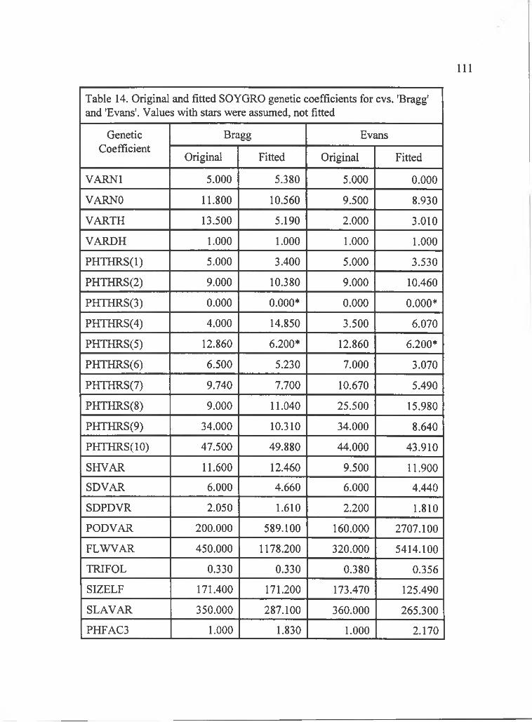
I l l
Table 14, Original and fitted SOYGRO genetic coefficients for cvs, 'Bragg' and 'Evans'. Values with stars were assumed, not fitted
GeneticCoefficient
Bragg Evans
Original Fitted Original Fitted
VARNl 5.000 5.380 5.000 0.000
VARNO 11.800 10.560 9.500 8.930
VARTH 13.500 5.190 2.000 3.010
VARDH 1.000 1.000 1.000 1.000
PHTHRS(l) 5.000 3.400 5.000 3.530
PHTHRS(2) 9.000 10.380 9.000 10.460
PHTHRS(3) 0.000 0.000* 0.000 0.000*
PHTHRS(4) 4.000 14.850 3.500 6.070
PHTHRS(5) 12.860 6.200* 12.860 6.200*
PHTHRS(6) 6.500 5.230 7.000 3.070
PHTHRS(7) 9.740 7.700 10.670 5.490
PHTHRS(8) 9.000 11.040 25.500 15.980
PHTHRS(9) 34.000 10.310 34.000 8.640
PHTHRS(IO) 47.500 49.880 44.000 43.910
SHVAR 11.600 12.460 9.500 11.900
SDVAR 6.000 4.660 6.000 4.440
SDPDVR 2.050 1.610 2.200 1.810
PODVAR 200.000 589.100 160.000 2707.100
FLWVAR 450.000 1178.200 320.000 5414.100
TRIFOL 0.330 0.330 0.380 0.356
SIZELF 171.400 171.200 173.470 125.490
SLAVAR 350.000 287.100 360.000 265.300
PHFAC3 1.000 1.830 1.000 2.170
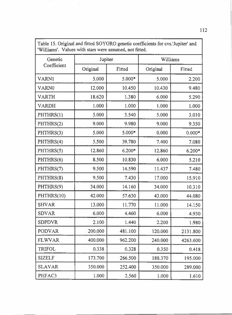
1 1 2
Table 15. Original and fitted SOYGRO genetic coefficients for cvs.'Jupiter' and 'Williams'. Values with stars were assumed, not fitted.
GeneticCoefficient
Jupiter Williams
Original Fitted Original Fitted
VARNl 5.000 5.000* 5.000 2.200
VARNO 12.000 10.450 10.430 9.480
VARTH 18.620 1.380 6.000 5.290
VARDH 1.000 1.000 1.000 1.000
PHTHRS(l) 5.000 3.540 5.000 3.010
PHTHRS(2) 9.000 9.980 9.000 9.350
PHTHRS(3) 5.000 5.000* 0.000 0.000*
PHTHRS(4) 5.500 39.780 7.400 7.080
PHTHRS(5) 12.860 6.200* 12.860 6.200*
PHTHRS(6) 8.500 10.830 6.000 5.210
PHTHRS(7) 9.500 14.590 11.437 7.480
PHTHRS(8) 9.500 7.430 17.000 15.910
PHTHRS(9) 34.000 14.160 34.000 10.310
PHTHRS(IO) 42.000 57.630 43.000 44.080
SHVAR 13.000 11.770 11.000 14.150
SDVAR 6.000 4.460 6.000 4.930
SDPDVR 2.100 1.440 2.200 1.980
PODVAR 200.000 481.100 120.000 2131.800
FLWVAR 400.000 962.200 240.000 4263.600
TRIFOL 0.338 0.328 0.350 0.418
SIZELF 173.700 266.500 188.370 195.000
SLAVAR 350.000 252.400 350.000 289.000
PHFAC3 1.000 2.560 1.000 1.610
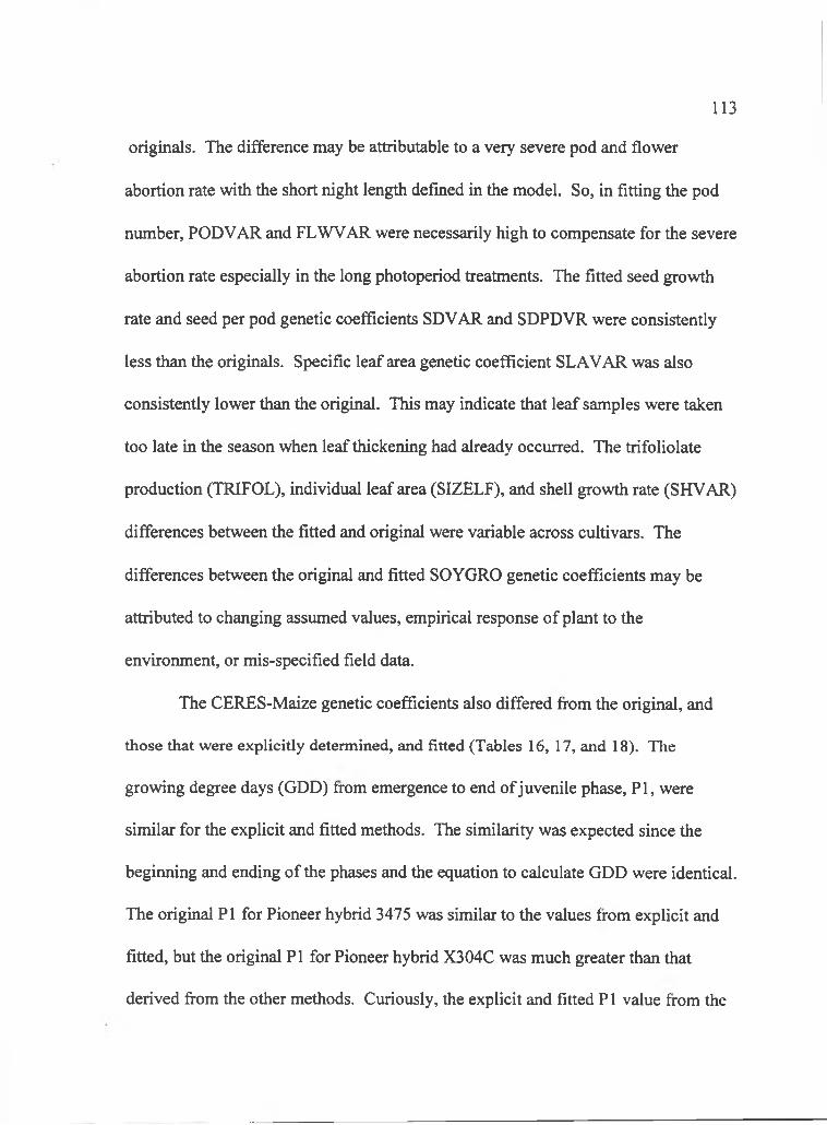
originals. The difference may be attributable to a very severe pod and flower
abortion rate with the short night length defined in the model. So, in fitting the pod
number, PODVAR and FLWVAR were necessarily high to compensate for the severe
abortion rate especially in the long photoperiod treatments. The fitted seed growth
rate and seed per pod genetic coefficients SDVAR and SDPDVR were consistently
less than the originals. Specific leaf area genetic coefficient SLAVAR was also
consistently lower than the original. This may indicate that leaf samples were taken
too late in the season when leaf thickening had already occurred. The trifoliolate
production (TRIFOL), individual leaf area (SIZELF), and shell growth rate (SHVAR)
differences between the fitted and original were variable across cultivars. The
differences between the original and fitted SOYGRO genetic coefficients may be
attributed to changing assmned values, empirical response of plant to the
environment, or mis-specified field data.
The CERES-Maize genetic coefficients also differed from the original, and
those that were explicitly determined, and fitted (Tables 16, 17, and 18). The
growing degree days (GDD) from emergence to end of juvenile phase, PI, were
similar for the explicit and fitted methods. The similarity was expected since the
beginning and ending of the phases and the equation to calculate GDD were identical.
The original PI for Pioneer hybrid 3475 was similar to the values from explicit and
fitted, but the original PI for Pioneer hybrid X304C was much greater than that
derived fi-om the other methods. Curiously, the explicit and fitted PI value from the
113
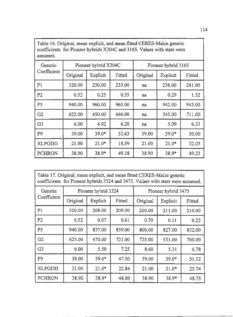
114
Table 16. Original, mean explicit, and mean fitted CERES-Maize genetic coefficients for Pioneer hybrids X304C and 3165. Values with stars were assumed.
GeneticCoefficient
Pioneer hybrid X304C Pioneer hybrid 3165
Original Explicit Fitted Original Explicit Fitted
PI 320.00 230.00 235.00 na 238.00 241.00
P2 0.52 0.25 0.35 na 0.29 1.52
P5 940.00 960.00 965.00 na 942.00 943.00
G2 625.00 450.00 646.00 na 545.00 711.00
G3 6.00 4.92 6.20 na 5.09 6.33
P9 39.00 39.0* 52.63 39.00 39.0* 50.00
XLPGDD 21.00 21.0* 18.59 21.00 21.0* 22.03
PCHRON 38.90 38.9* 49.18 38.90 38.9* 49.23
Table 17. Original, mean explicit, and mean fitted CERES-Maize genetic coefficients for Pioneer hybrids 3324 and 3475. Values with stars were assumed.
GeneticCoefficient
Pioneer hybrid 3324 Pioneer hybrid 3475
Original Explicit Fitted Original Explicit Fitted
PI 320.00 208.00 209.00 200.00 211.00 210.00
P2 0.52 0.07 0.61 0.70 0.11 0.22
P5 940.00 837.00 859.00 800.00 827.00 832.00
G2 625.00 470.00 721.00 725.00 531.00 760.00
G3 6.00 5.50 7.25 8.60 5.31 6.78
P9 39.00 39.0* 47.50 39.00 39.0* 51.32
XLPGDD 21.00 21.0* 22.84 21.00 21.0* 25.74
PCHRON 38.90 38.9* 48.80 38.90 38.9* 48.75
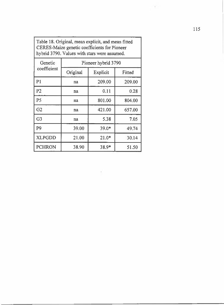
115
Table 18. Original, mean explicit, and mean fitted CERES-Maize genetic coefficients for Pioneer hybrid 3790. Values with stars were assumed.
Geneticcoefficient
Pioneer hybrid 3790
Original Explicit Fitted
PI na 209.00 209.00
P2 na 0.11 0.28
P5 na 801.00 804.00
G2 na 421.00 657.00
G3 na 5.38 7.05
P9 39.00 39.0* 49.74
XLPGDD 21.00 21.0* 30.14
PCHRON 38.90 38.9* 51.50

winter planting was very similar to the original PI for Pioneer hybrid X304C (data
not shown). The photoperiod sensitivity genetic coefficient, P2, was highly variable
among the three types of genetic coefficients. Generally, the original P2 had the
highest value, followed by the fitted, then explicit. The explicit may have been
lowest because the regression line was not forced through an intercept, whereas the
fitted method effectively forced a line through the point at 12.5 h. The GDD from
silking to physiological maturity, P5, was similar among those that were explicit and
fitted. The similarity may be that the beginning and ending stages, and the GDD
calculation for both methods were the same. The potential number o f kernels per
plant and the kernel growth rate, G2 and G3, were lower for the explicit than the
fitted. The lower explicit G2 and G3 may indicate that there were non-ideal
conditions for kernel development in the field, at least in some cases. A possible non
ideal condition may be temperature. Linear regression of G3 on mean daily
temperature during kernel growth was described as y = 0.45 x - 4.51, r = 0.55
(n=158), where y was G3 and x was temperature. This indicates G3 varies as a
function of temperature and is not an environment independent constant. The GDD
from germination to emergence and to fully expand one leaf, P9 and PCHRON, was
greater for fitted than the original values. GDD to produce a leaf primordia during
the phase from germination to tassel initiation, XLPGDD, varied from 18.59 to 30.14
among the hybrids while the original value was a constant 21.
116

The factors that affected the SOYGRO and CERES-Maize genetic
coefficients derived from the fitting and explicit method were identified with analysis
o f variance. If the genetic coefficients and the model well simulated the soybean
growth and development and the genetic coefficient derivation method was sound,
then the only significant source of variation would be the difference among cuitivars.
Any other significant source of variation would indicate shortcomings of the field
data, genetic coefficient estimation method, or the model.
The SOYGRO development genetic coefficients PHTHRS 1 and PHTHRS 2,
the thermal time from planting to emergence and planting to unifoliolate, had site and
cultivar as significant sources of variation (Table 19). The PHTHRS 1 value was
higher at the warmer site, Kuiaha, than the cooler site, Haleakala, 3.33 compared to
2.65. The opposite effect of site was observed in PHTHRS 2 values: 9.5 at the warm
site and 10.1 at the cool site. The paradoxical results may be an artifact of where
temperature was measured versus the temperature that was more related to
development. From planting to emergence, development rate should be related to soil
temperature, but air temperature was used to calculate thermal time. The mean soil
and air temperature was 24.26 and 20.24 °C at the cool site, and 23.50 and 21.73 °C
at the warm site. The difference in soil and air temperature suggested that the plant
was developing quickly at the cool site, but the thermal time was accumulating
relatively slowly due to the much lower air temperature. Hence, the thermal time
from planting to emergence was greater at the cool than at the warm site. However,
117
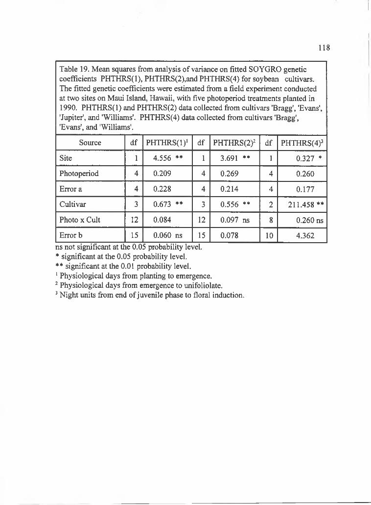
118
Table 19. Mean squares from analysis of variance on fitted SOYGRO genetic coefficients PHTHRS(l), PHTHRS(2),and PHTHRS(4) for soybean cultivars. The fitted genetic coefficients were estimated from a field experiment conducted at two sites on Maui Island, Hawaii, with five photoperiod treatments planted in 1990. PHTHRS(l) and PHTHRS(2) data collected from cultivars 'Bragg', 'Evans', 'Jupiter', and 'Williams'. PHTHRS(4) data collected from cultivars 'Bragg', 'Evans', and 'Williams'.
Source df PHTHRS(l)* df PHTHRS(2)2 df PHTHRS(4)^
Site 1 4.556 ** 1 3.691 ** 1 0.327 *
Photoperiod 4 0.209 4 0.269 4 0.260
Error a 4 0.228 4 0.214 4 0.177
Cultivar 3 0.673 ** 3 0.556 ** 2 211.458 **
Photo X Cult 12 0.084 12 0.097 ns 8 0.260 ns
Error b 15 0.060 ns 15 0.078 10 4.362ns not significant at the 0.05 probability level.* significant at the 0.05 probability level.** significant at the 0.01 probability level.‘ Physiological days from planting to emergence.’ Physiological days from emergence to unifoliolate. Night units from end o f juvenile phase to floral induction.
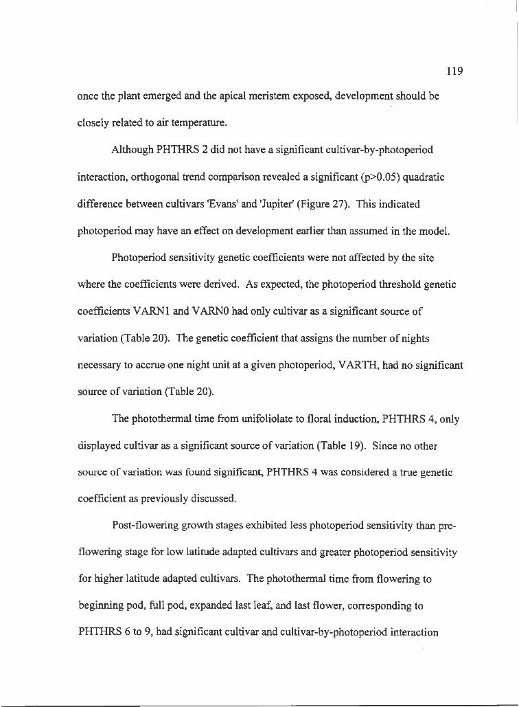
once the plant emerged and the apical meristem exposed, development should be
closely related to air temperature.
Although PHTHRS 2 did not have a significant cultivar-by-photoperiod
interaction, orthogonal trend comparison revealed a significant (p>0.05) quadratic
difference between cultivars 'Evans' and 'Jupiter' (Figure 27). This indicated
photoperiod may have an effect on development earlier than assumed in the model.
Photoperiod sensitivity genetic coefficients were not affected by the site
where the coefficients were derived. As expected, the photoperiod threshold genetic
coefficients VARNl and VARNO had only cultivar as a significant source of
variation (Table 20). The genetic coefficient that assigns the number of nights
necessary to accrue one night unit at a given photoperiod, VARTH, had no significant
source of variation (Table 20).
The photothermal time from unifoliolate to floral induction, PHTHRS 4, only
displayed cultivar as a significant source of variation (Table 19). Since no other
source of variation was found significant, PHTHRS 4 was considered a true genetic
coefficient as previously discussed.
Post-flowering growth stages exhibited less photoperiod sensitivity than pre
flowering stage for low latitude adapted cultivars and greater photoperiod sensitivity
for higher latitude adapted cultivars. The photothermal time from flowering to
beginning pod, full pod, expanded last leaf, and last flower, corresponding to
PHTHRS 6 to 9, had significant cultivar and cultivar-by-photoperiod interaction
119
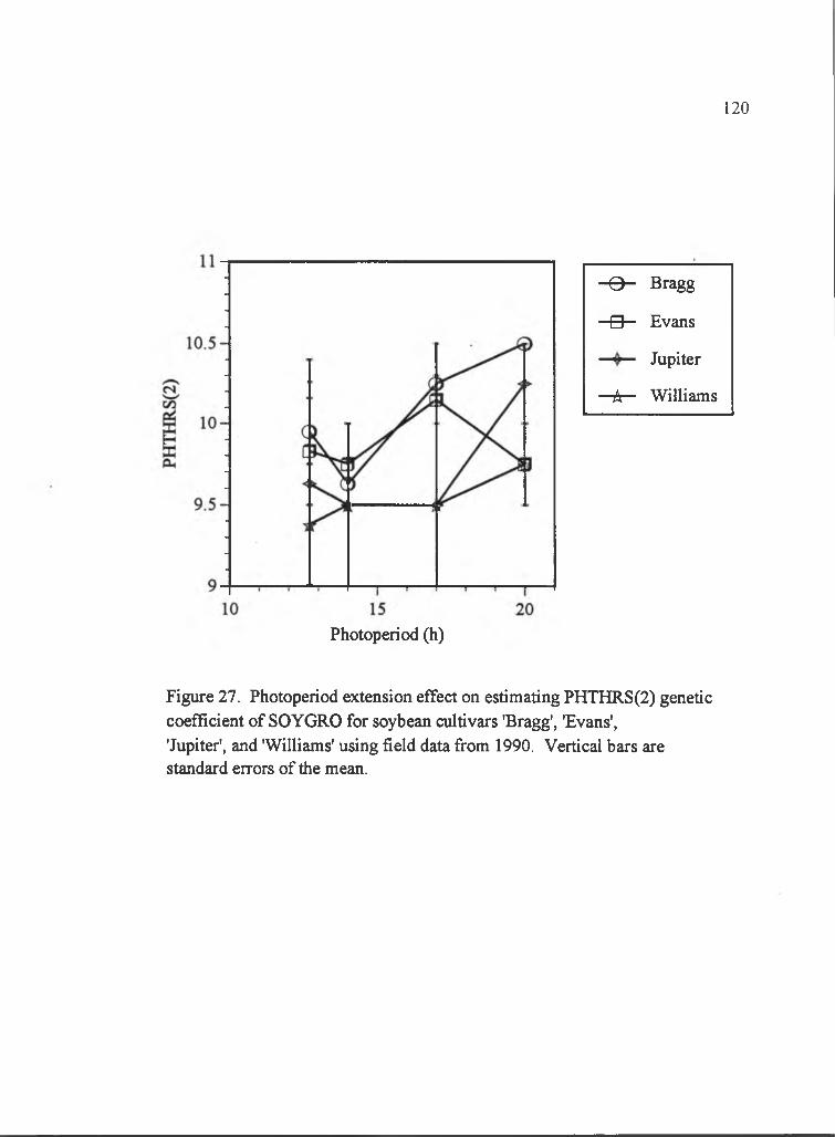
120
- 0 - Bragg
- e - Evans
Jupiter
- A - Williams
Photoperiod (h)
Figure 27. Photoperiod extension effect on estimating PHTHRS(2) genetic coefficient of SOYGRO for soybean cultivars 'Bragg', 'Evans','Jupiter', and 'Williams' using field data from 1990. Vertical bars are standard errors of the mean.
121
Table 20. Mean squares from analysis of variance on fitted SOYGRO genetic coefficients VARTH, VARNl, VARNO for soybean cultivars 'Bragg', 'Evans', and 'Williams' estimated from two sites on Maui Island, Hawaii, under five photoperiod treatments in 1990.
Source df VARTH ' df VARNl 2 df VARNO^
Site 1 0.928 ns 1 0.180 ns 1 0.470 ns
Cultivar 2 2.060 ns 2 14.618 * 2 7.007 **
Error 2 0.461 ns 2 0.802 2 0.077ns not significant at the 0.05 probability level.* significant at the 0.05 probability level.' Maximum night units threshold, night accumulator units. Lower nightlength threshold, h. Upper nightlength threshold, h.

sources of variation (Tables 21 and 22). Orthogonal trend comparisons showed that
cultivar 'Bragg', 'Evans', and 'Williams' had significantly (p>0.05) different linear
trends one from another. The general trend was the low latitude adapted cultivar
'Bragg' had decreased photothermal time value as photoperiod increased, while the
high latitude adapted cultivar 'Evans' had increased photothermal time value (figures
28 to 31). The mid-latitude adapted cultivar 'Williams' had intermediate linear trend.
The decreased photothermal time value as photoperiod increased indicated the
photoperiod sensitivity in the model was too great for the particular phase, so a
decreased photothermal value was needed to correctly estimate the stage occurrence
in the field. Similarly, the increased photothermal time value indicated photoperiod
sensitivity was too small in the model.
Photothermal time from flowering to physiological maturity, PHTHRS(IO),
was related to photoperiod. The cultivar-by-photoperiod interaction was a significant
source of variation for PHTHRS(IO) (Table 22). The interaction resulted from a
highly significant (p>0.01) difference in quadratic trends between soybean cuitivars
'Evans' and 'Williams' (Figure 32). The trend with photoperiod indicated the pre
flowering photoperiod sensitivity did not adequately describe sensitivity in the
present phase.
Site had an effect on the number of trifoliolates produced in one physiological
day, TRIFOL, for soybean cultivar 'Bragg', but no effect for cultivar 'Evans' (Table
23). The TRIFOL value for the cool site was greater than at the warm site for cultivar
1 2 2
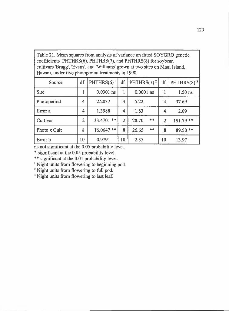
123
Table 21. Mean squares from analysis of variance on fitted SOYGRO genetic coefficients PHTHRS(6), PHTHRS(7), and PHTHRS(8) for soybean cultivars 'Bragg', 'Evans', and 'Williams' grown at two sites on Maui Island, Hawaii, under five photoperiod treatments in 1990.
Source df PHTHRS(6)‘ df PHTHRS(7)' df PHTHRS(8) ^
Site 1 0.0301 ns 1 0.0001 ns 1 1.50 ns
Photoperiod 4 2.2037 4 5.22 4 37.69
Error a 4 1.3988 4 1.63 4 2.09
Cultivar 2 33.4701 ** 2 28.70 ** 2 191.79**
Photo X Cult 8 16.0647 ** 8 26.65 ** 8 89.50 **
Error b 10 0.9791 10 2.35 10 13.97ns not significant at the 0.05 probability level. * significant at the 0.05 probability level.** significant at the 0.01 probability level.' Night units from flowering to beginning pod. Night units from flowering to full pod. Night units fi-om flowering to last leaf
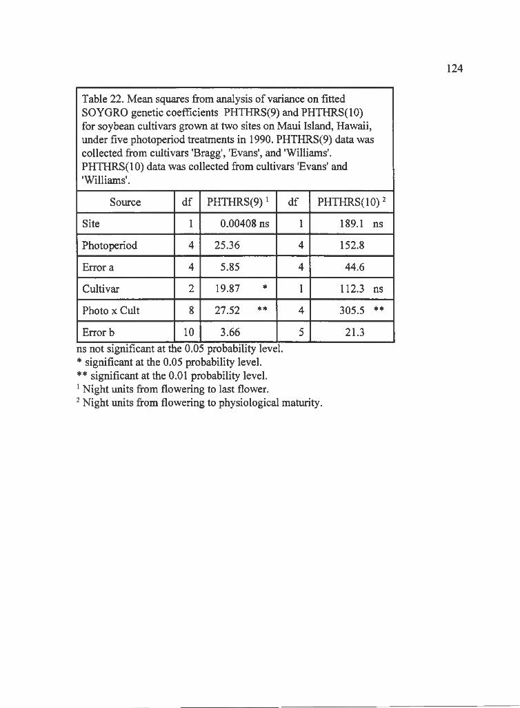
124
Table 22. Mean squares fi-om analysis of variance on fitted SOYGRO genetic coefficients PHTHRS(9) and PHTHRS(IO) for soybean cultivars grown at two sites on Maui Island, Hawaii, under five photoperiod treatments in 1990. PHTHRS(9) data was collected from cultivars 'Bragg', 'Evans', and 'Williams'. PHTHRS(IO) data was collected fi-om cultivars 'Evans' and 'Williams'.
Source df PHTHRS(9) * df PHTHRS(IO)’
Site 1 0.00408 ns 1 189.1 ns
Photoperiod 4 25.36 4 152.8
Error a 4 5.85 4 44.6
Cultivar 2 19.87 * 1 112.3 ns
Photo X Cult 8 27.52 ** 4 305.5 **
Error b 10 3.66 5 21.3ns not significant at the 0.05 probability level.* significant at the 0.05 probability level.** significant at the 0.01 probability level.‘ Night units from flowering to last flower.’ Night units from flowering to physiological maturity.
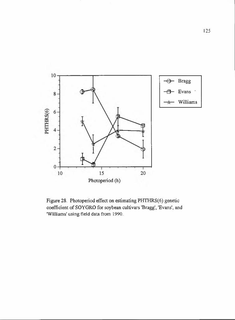
125
- 0 - Bragg
- 9 — Evans '
- k ~ Williams
Photoperiod (h)
Figure 28. Photoperiod effect on estimating PHTHRS(6) genetic coefficient of SOYGRO for soybean cultivars 'Bragg', 'Evans', and 'Williams' using field data from 1990.
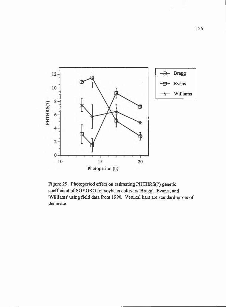
126
- 0 - Bragg
- 9 — Evans
-k— Williams
Photoperiod (h)
Figure 29. Photoperiod effect on estimating PHTHRS(7) genetic coefficient of SOYGRO for soybean cultivars 'Bragg', 'Evans', and 'Williams' using field data from 1990. Vertical bars are standard errors of the mean.
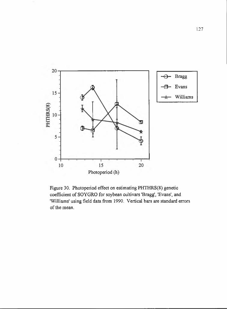
127
- 0 - Bragg
- 0 Evans
- A - Williams
Photoperiod (h)
Figure 30. Photoperiod effect on estimating PHTHRS(8) genetic coefficient of SOYGRO for soybean cultivars 'Bragg', 'Evans', and 'Williams' using field data from 1990. Vertical bars are standard errors of the mean.
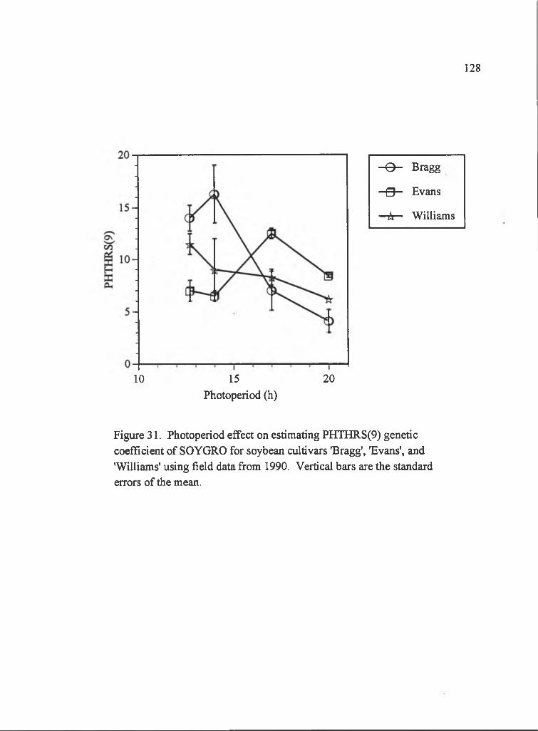
128
10 15Photoperiod (h)
20
- 0 - Bragg
- 9 — Evans
-A— Williams
Figure 31. Photoperiod effect on estimating PHTHRS(9) genetic coefficient of SOYGRO for soybean cultivars 'Bragg', 'Evans', and 'Williams' using field data from 1990. Vertical bars are the standard errors of the mean.
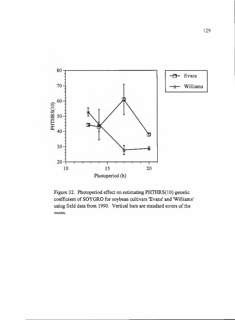
129
oS '
10
- 0 - Evans
-A— Williams
15Photoperiod (h)
20
Figure 32. Photoperiod effect on estimating PHTHRS(IO) genetic coefficient of SOYGRO for soybean cultivars 'Evans' and 'Williams' using field data from 1990. Vertical bars are standard errors of the mean.
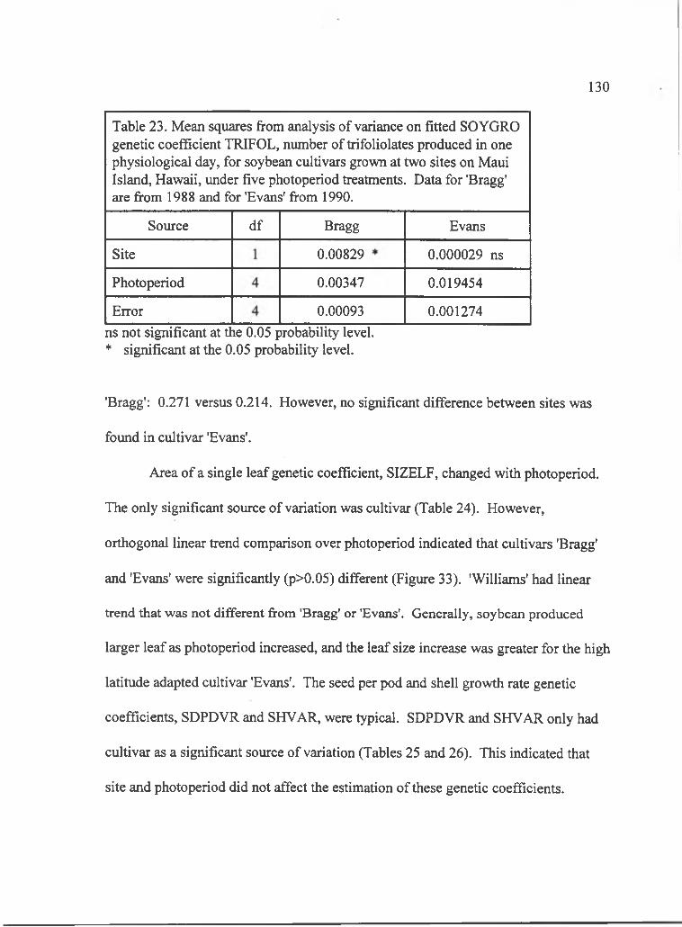
130
Table 23. Mean squares from analysis of variance on fitted SOYGRO genetic coefficient TRIFOL, number of trifoliolates produced in one physiological day, for soybean cultivars grown at two sites on Maui Island, Hawaii, under five photoperiod treatments. Data for 'Bragg' are from 1988 and for 'Evans' from 1990.
Source df Bragg Evans
Site 0.00829 0.000029 ns
Photoperiod 0.00347 0.019454
Error 0.00093 0.001274ns not significant at the 0.05 probability level. * significant at the 0.05 probability level.
'Bragg': 0.271 versus 0.214. However, no significant difference between sites was
found in cultivar 'Evans'.
Area of a single leaf genetic coefficient, SIZELF, changed with photoperiod.
The only significant source of variation was cultivar (Table 24). However,
orthogonal linear trend comparison over photoperiod indicated that cultivars 'Bragg'
and 'Evans' were significantly (p>0.05) different (Figure 33). 'Williams' had linear
trend that was not different from 'Bragg' or 'Evans'. Generally, soybean produced
larger leaf as photoperiod increased, and the leaf size increase was greater for the high
latitude adapted cultivar 'Evans'. The seed per pod and shell growth rate genetic
coefficients, SDPDVR and SHVAR, were typical. SDPDVR and SHVAR only had
cultivar as a significant source of variation (Tables 25 and 26). This indicated that
site and photoperiod did not affect the estimation of these genetic coefficients.
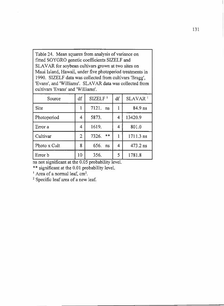
131
Table 24. Mean squares firom analysis of variance on fitted SOYGRO genetic coefficients SIZELF and SLAVAR for soybean cultivars grown at two sites on Maui Island, Hawaii, under five photoperiod treatments in 1990. SIZELF data was collected from cultivars 'Bragg', 'Evans', and 'Williams'. SLAVAR data was collected from cultivars 'Evans' and 'Williams'.
Source df SIZELF ' df SLAVAR'
Site 1 7121. ns 1 84.9 ns
Photoperiod 4 5873. 4 13420.9
Error a 4 1619. 4 801.0
Cultivar 2 7326. ** 1 1711.3 ns
Photo X Cult 8 656. ns 4 473.2 ns
Error b 10 356. 5 1781.8ns not significant at the O.C5 probability level.** significant at the 0.01 probability level. ' Area of a normal leaf, cm’.’ Specific leaf area of a new leaf.
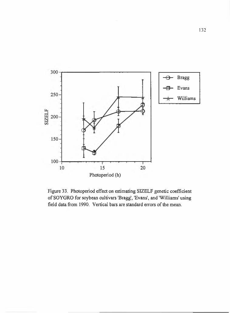
132
■O- Bragg
- 9 - Evans
-k— Williams
Photoperiod (h)
Figure 33. Photoperiod effect on estimating SIZELF genetic coefficient of SOYGRO for soybean cultivars 'Bragg', 'Evans', and 'Williams' using field data from 1990. Vertical bars are standard errors of the mean.
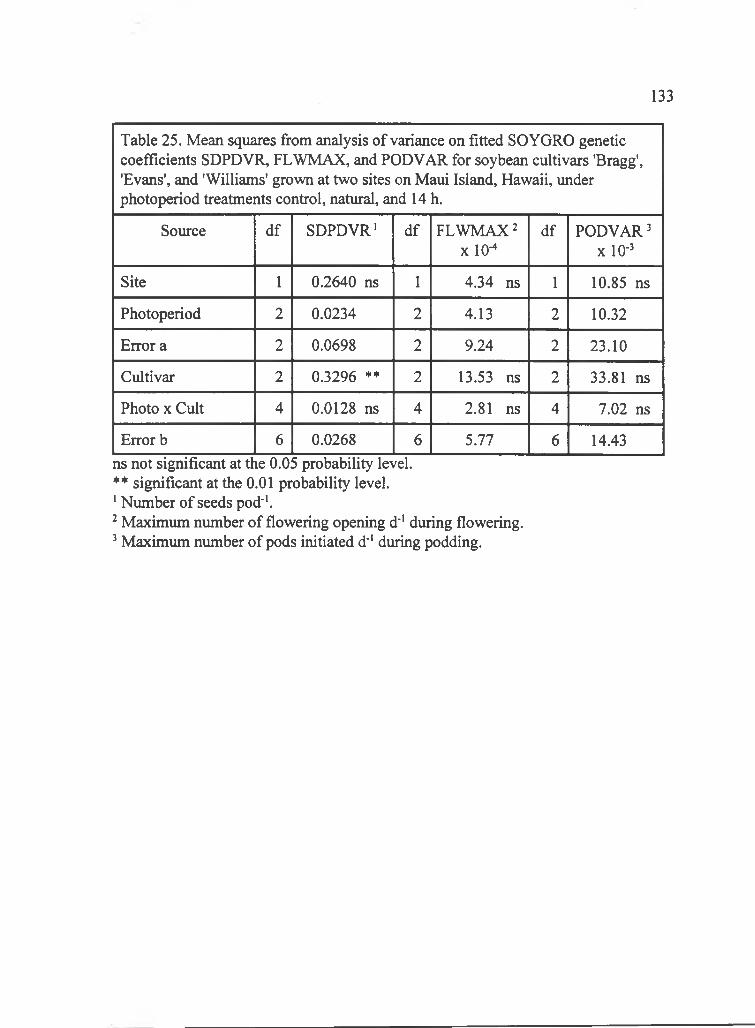
133
Table 25. Mean squares from analysis of variance on fitted SOYGRO genetic coefficients SDPDVR, FLWMAX, and PODVAR for soybean cultivars 'Bragg', 'Evans', and 'Williams' grown at two sites on Maui Island, Hawaii, under photoperiod treatments control, natural, and 14 h.
Source df SDPDVR' df FLWMAX 2X 10-
df PODVAR ^X 10-'
Site 1 0.2640 ns 1 4.34 ns 1 10.85 ns
Photoperiod 2 0.0234 2 4.13 2 10.32
Error a 2 0.0698 2 9.24 2 23.10
Cultivar 2 0.3296 ** 2 13.53 ns 2 33.81 ns
Photo X Cult 4 0.0128 ns 4 2.81 ns 4 7.02 ns
Error b 6 0.0268 6 5.77 6 14.43ns not significant at the 0.05 probability level.** significant at the 0.01 probability level.' Number o f seeds pod''. Maximum number of flowering opening d'' during flowering. Maximum number of pods initiated d'' during podding.
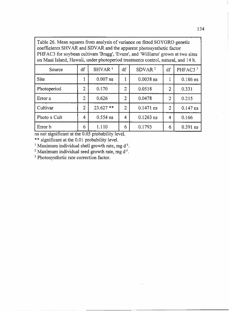
134
Table 26. Mean squares from analysis of variance on fitted SOYGRO genetic coefficients SHVAR and SDVAR and the apparent photosynthetic factor PHFAC3 for soybean cuitivars 'Bragg', 'Evans', and 'Williams' grown at two sites on Maui Island, Hawaii, under photoperiod treatments control, natural, and 14 h.
Source df SHVAR* df SDVAR 2 df PHFAC3'
Site 1 0.007 ns 1 0.0038 ns 1 0.186 ns
Photoperiod 2 0.170 2 0.0518 2 0.331
Error a 2 0.626 2 0.0478 2 0.215
Cultivar 2 23.627 ** 2 0.1471 ns 2 0.147 ns
Photo X Cult 4 0.554 ns 4 0.1263 ns 4 0.166
Error b 6 1.110 6 0.1793 6 0.391 nsns not significant at the 0.05 probability level. ** significant at the 0.01 probability level.' Maximum individual shell growth rate, mg d '. Maximum individual seed growth rate, mg d’*.
' Photosynthetic rate correction factor.

Site, photoperiod, and cultivar did not affect the estimation of the genetic
coefficients that determine specific leaf area (SLAVAR), maximum number of
flowers per day (FLWVAR), maximum number of pods per day (PODVAR), and
seed growth rate (SDVAR), and the photosynthetic rate factor (PHFAC3). In the
analysis of variance, SLAVAR, FLWVAR, PODVAR, SDVAR, and PHFAC3 were
not significantly different among sites, cultivars, and interaction between cultivar and
photoperiod (Tables 24, 25,26). The lack of significance may be due to
independence of these coefficients from environmental and genotype factors, or
imprecision in the experimental results.
Explicitly estimated genetic coefficients for CERES-Maize displayed some
dependence on environment. The genetic coefficient that determined the thermal
time from emergence to end of juvenile phase, PI, had significant year, cultivar, and
cultivar-by-year interaction sources of variation (Table 27). The significant effect of
year resulted from PI values of 168 and 270 in 1989 and 1991, respectively. The
difference in PI values may be attributed to where temperature was measured. Air
temperature was used to calculate thermal time for development from emergence to
end of juvenile phase. However, soil temperature may be more closely related to
development rate during this phase. Then, using the current calculation for PI, the
difference in soil and air temperature can cause variation in PI because thermal time
will accumulate according to air temperature while soil temperature determines
development rate. The soil temperature at 10 cm depth and air temperaPire was 23.4
135
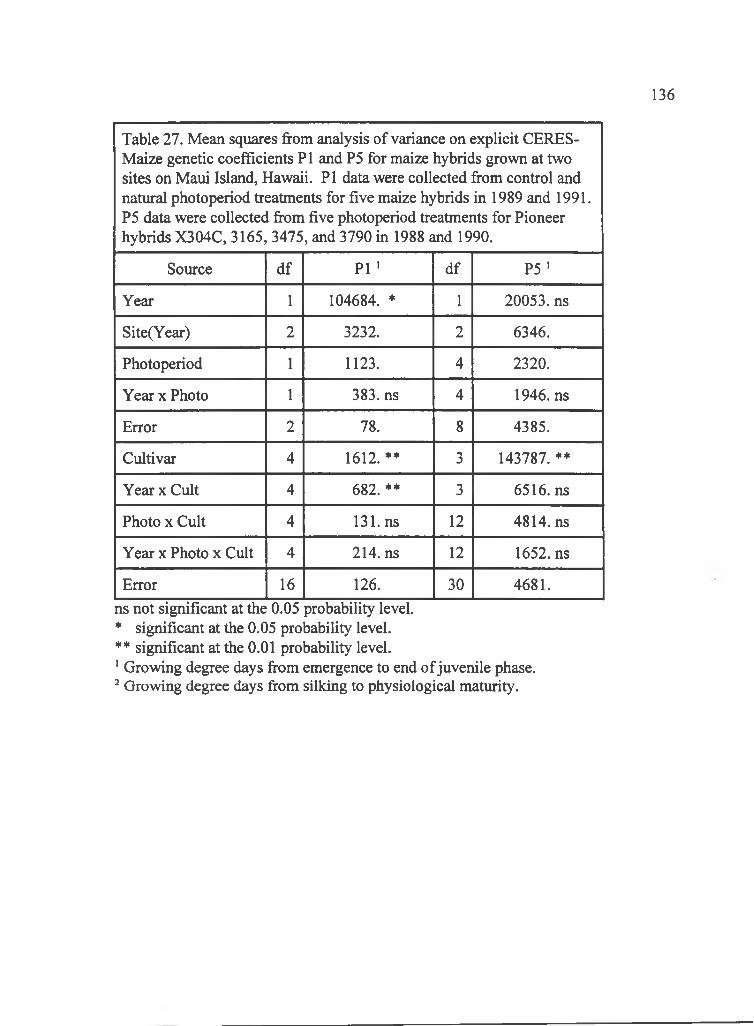
136
Table 27. Mean squares from analysis of variance on explicit CERES- Maize genetic coefficients PI and P5 for maize hybrids grown at two sites on Maui Island, Hawaii. PI data were collected from control and natural photoperiod treatments for five maize hybrids in 1989 and 1991. P5 data were collected from five photoperiod treatments for Pioneer hybrids X304C, 3165, 3475, and 3790 in 1988 and 1990.
Source df PI ' df P5 '
Year 1 104684. ♦ 1 20053. ns
Site(Year) 2 3232. 2 6346.
Photoperiod 1 1123. 4 2320.
Year x Photo 1 383. ns 4 1946. ns
Error 2 78. 8 4385.
Cultivar 4 1612.** 3 143787. **
Year X Cult 4 682.** 3 6516. ns
Photo X Cult 4 131. ns 12 4814. ns
Year X Photo x Cult 4 214. ns 12 1652. ns
Error 16 126. 30 4681.ns not significant at the 0.05 probability level.* significant at the 0.05 probability level.** significant at the 0.01 probability level.' Growing degree days from emergence to end of juvenile phase. Growing degree days from silking to physiological maturity.

°C and 21.3 °C in 1989 and 19.7 °C and 18.5 °C in 1991 during the first month after
planting. The larger difference between soil and air temperatures indicated that less
thermal time was accumulating while development was proceeding at a high rate in
1989. Therefore, the PI value was less in 1989 than in 1991. There was a cultivar-
by-year interaction that seemed to result from Pioneer hybrid 3165 accumulating
more thermal time in 1991 than the other hybrids (figure 34).
The explicitly estimated photoperiod sensitivity genetic coefficient for
CERES-Maize, P2, did not display any significant source of variation (Table 28).
The lack o f any significant factor to affect P2 may have been due to imprecision in
the experimental design.
Explicitly calculated genetic coefficient that determined thermal time from
silking to physiological maturity, P5, showed dependence on genotype. The
significantly different P5 values among hybrids indicated that the time from silking to
physiological maturity was only dependent on genotype (Table 27). However,
orthogonal linear trend comparisons over photoperiod indicated that Pioneer hybrid
X304C was different from Pioneer hybrids 3165 and 3475 (Figure 35). Yet, Pioneer
hybrids 3165, 3475, and 3790 did not have significantly different linear trends over
photoperiods.
The explicitly estimated number of kernels per plant genetic coefficient, G2,
for the tropically adapted hybrid was highly sensitive to photoperiod. The significant
sources of variation for G2 were cultivar and photoperiod-by-cultivar interaction
137
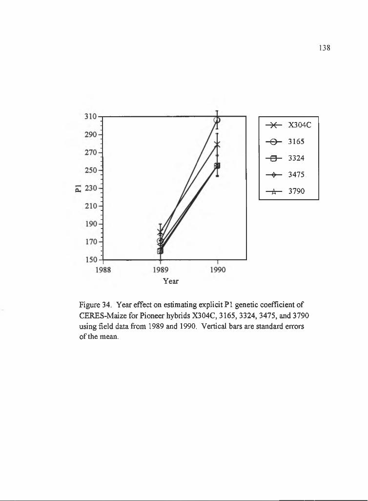
138
- X - X304C
- 0 - 3165
- g - 3324
0 — 3475
T$r- 3790
Year
Figure 34. Year effect on estimating explicit PI genetic coefficient of CERES-Maize for Pioneer hybrids X304C, 3165, 3324, 3475, and 3790 using field data from 1989 and 1990. Vertical bars are standard errors of the mean.
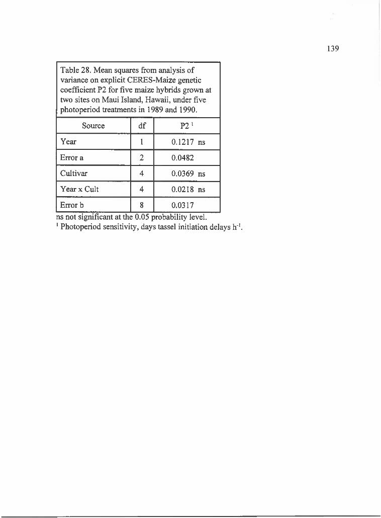
139
Table 28. Mean squares from analysis of variance on explicit CERES-Maize genetic coefficient P2 for five maize hybrids grown at two sites on Maui Island, Hawaii, under five photoperiod treatments in 1989 and 1990.
Source df P 2 '
Year 1 0.1217 ns
Error a 2 0.0482
Cultivar 4 0.0369 ns
Year x Cult 4 0.0218 ns
Error b 8 0.0317ns not significant at the 0.05 probability level.' Photoperiod sensitivity, days tassel initiation delays h'*.
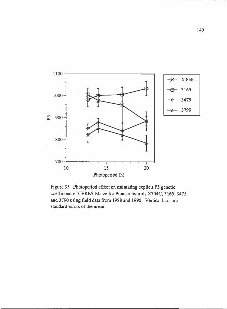
140
-X“ X304C
- 0 - 3165
■ 0 - 3475
-A - 3790
10 15Photoperiod (h)
20
Figure 35. Photoperiod effect on estimating explicit P5 genetic coefficient of CERES-Maize for Pioneer hybrids X304C, 3165, 3475, and 3790 using field data from 1988 and 1990. Vertical bars are standard errors of the mean.

(Table 29). Orthogonal linear trends over photoperiod indicated that the negative
slope for Pioneer hybrid X304C was highly significantly different (p>0.01) from the
other three hybrids that were fairly constant (Figure 36). The decreasing number of
kernels was attributable to the increasing silking-tasseling interval with longer
photoperiod that disrupted pollination for Pioneer hybrid X304C (Manrique and
Hodges, 1991).
The kernel number response to photoperiod affected the explicitly estimated
kernel growth rate genetic coefficient, G3. Although no significant sources of
variation were found for G3 (Table 29), orthogonal linear trend over photoperiod
revealed that only Pioneer hybrid X304C was different (p>0.01, p>0.05) compared to
Pioneer hybrid 3165 and 3475 (Figure 37). While Pioneer hybrids 3165, 3475, and
3790 had reduced G3 as photoperiod increased. Pioneer hybrid X304C had increased
G3. The increase in kernel growth rate for Pioneer hybrid can be due to the decrease
in kernel number that allowed more available photosynthate to increase the size of
the fewer pollinated kernels (Schoper et al., 1982) in a shorter filling period (Figure
35). Then, the effect photoperiod on kernel growth rate would be related to the
photoperiod effect on kernel number.
The fitted CERES-Maize genetic coefficients that determine the thermal time
from planting to emergence, PI, and from silking to physiological maturity, P5,
showed similar dependence on environment as the explicitly calculated ones. Fitted
PI had significant year, cultivar, and year-by-cultivar interaction sources of variation
141
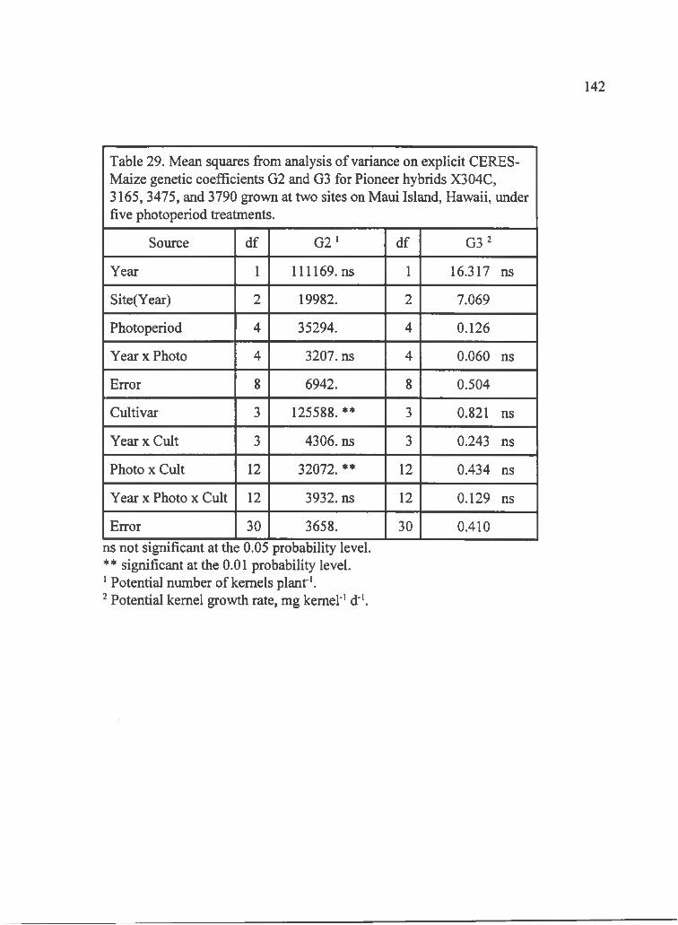
142
Table 29. Mean squares from analysis of variance on explicit CERES- Maize genetic coefficients G2 and G3 for Pioneer hybrids X304C,3165, 3475, and 3790 grown at two sites on Maui Island, Hawaii, under five photoperiod treatments.
Source df G 2 ' df G3^
Year 1 111169. ns 1 16.317 ns
Site(Year) 2 19982. 2 7.069
Photoperiod 4 35294. 4 0.126
Year x Photo 4 3207. ns 4 0.060 ns
Error 8 6942. 8 0.504
Cultivar 3 125588. ** 3 0.821 ns
Year x Cult 3 4306. ns 3 0.243 ns
Photo X Cult 12 32072. *♦ 12 0.434 ns
Year X Photo x Cult 12 3932. ns 12 0.129 ns
Error 30 3658. 30 0.410ns not significant at the 0.05 probability level. ** significant at the 0.01 probability level.' Potential number of kernels plant"'. Potential kernel growth rate, mg kernel"' d"'.
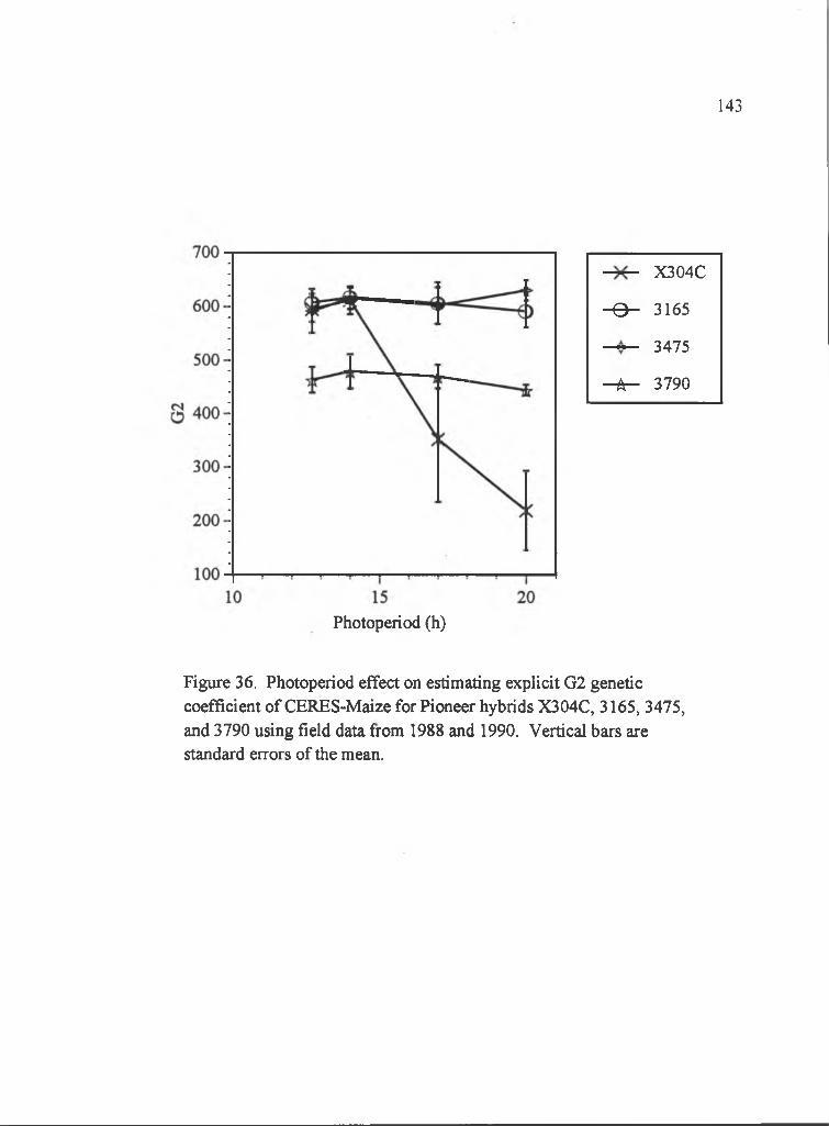
143
X304C
- 9 - 3165
3475
- A - 3790
Photoperiod (h)
Figure 36. Photoperiod effect on estimating explicit G2 genetic coefficient of CERES-Maize for Pioneer hybrids X304C, 3165, 3475, and 3790 using field data from 1988 and 1990. Vertical bars are standard errors of the mean.
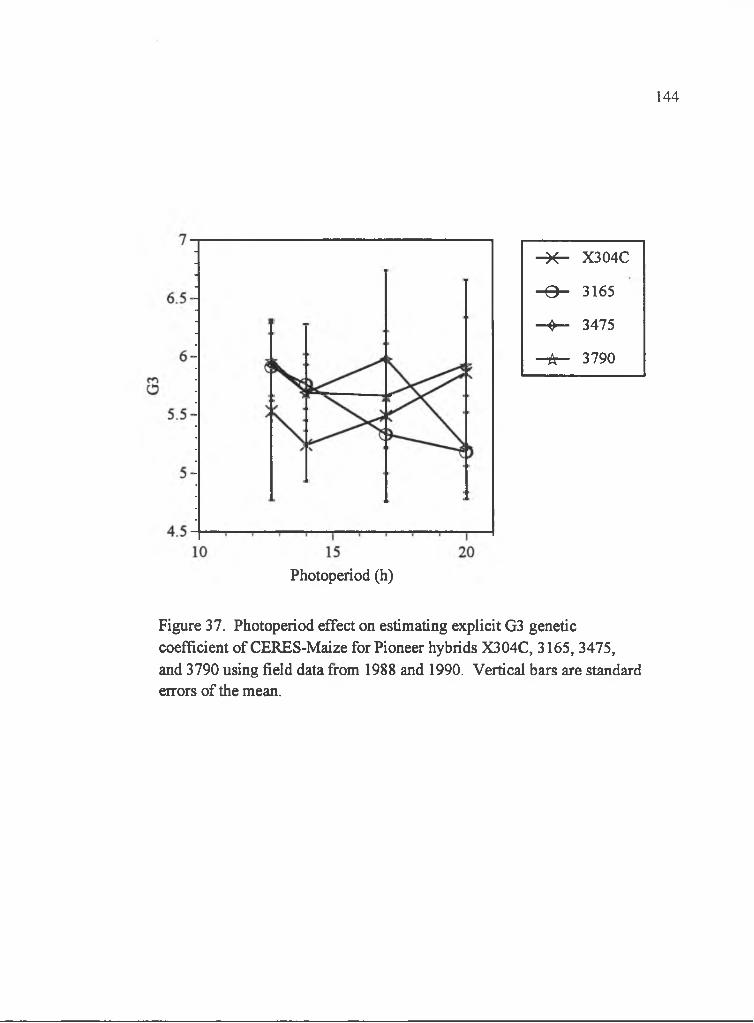
144
- 0 - X304C
- 0 - 3165
0 - 3475
-k- 3790
Photoperiod (h)
Figure 37. Photoperiod effect on estimating explicit G3 genetic coefficient of CERES-Maize for Pioneer hybrids X304C, 3165, 3475, and 3790 using field data from 1988 and 1990. Vertical bars are standard errors of the mean.

(Table 30). The year-by-cultivar interaction resulted from Pioneer hybrid 3165
responding differently to year from the other hybrids (figure 38). Fitted P5 had
cultivar as a significant source of variation (Table 30). While there was no significant
photoperiod-by-cultivar interaction, orthogonal linear trend comparison over
photoperiod revealed that Pioneer hybrid X304C was highly significantly (p>0.01)
different from Pioneer hybrids 3165 and 3475 (figure 39). These results for the fitted
PI and P5 are almost identical to the explicitly calculated genetic coefficients. The
similar results between the two methods were a consequence of using the same
thermal time equation, temperature data, and dates to calculate the genetic
coefficients.
Values for the fitted photoperiod sensitivity genetic coefficient, P2, were
dependent on photoperiod. P2 had a highly significant (p>0.01) cultivar effect (Table
31). There was no significant photoperiod-by-cultivar interaction effect, but
orthogonal linear trend over photoperiod comparisons showed significant differences
between Pioneer hybrids X304C and 3165, 3165 and 3475, and 3165 and 3790
(figure 40). The P2 trend over photoperiod may be caused by the model assumption
that the threshold photoperiod for delaying tassel initiation is 12.5 h. If the true
threshold photoperiod were less than 12.5 h, then fitting the P2 value to match tassel
initiation would be very large to correct for the delay already imposed by photoperiod
below 12.5 h (figure 41). Furthermore, photoperiods close to 12.5 h would have large
P2 values and decrease as photoperiod increased. This relationship of decreasing P2
145
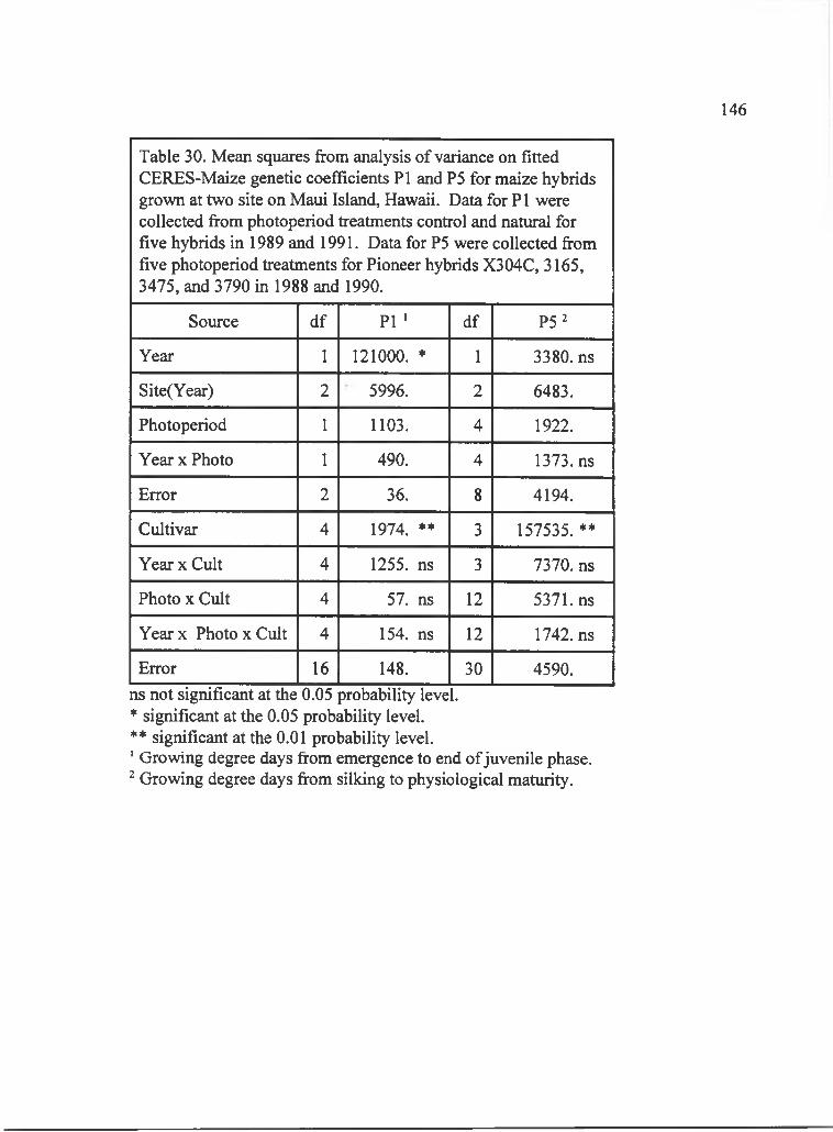
146
Table 30. Mean squares from analysis of variance on fitted CERES-Maize genetic coefficients PI and P5 for maize hybrids grown at two site on Maui Island, Hawaii. Data for PI were collected from photoperiod treatments control and natural for five hybrids in 1989 and 1991. Data for P5 were collected from five photoperiod treatments for Pioneer hybrids X304C, 3165, 3475, and 3790 in 1988 and 1990.
Source df PI ' df P5^
Year 1 121000. * 1 3380. ns
Site(Year) 2 5996. 2 6483.
Photoperiod 1 1103. 4 1922.
Year X Photo 1 490. 4 1373. ns
Error 2 36. 8 4194.
Cultivar 4 1974. ** 3 157535. **
Year X Cult 4 1255. ns 3 7370. ns
Photo X Cult 4 57. ns 12 5371. ns
Y earx Photo x Cult 4 154. ns 12 1742. ns
Error 16 148. 30 4590.ns not significant at the 0.05 probability level.* significant at the 0.05 probability level.** significant at the 0.01 probability level.' Growing degree days from emergence to end of juvenile phase. Growing degree days from silking to physiological maturity.

147
X304C
- 0 - 3165
- e - 3324
0 - 3475
-A - 3790
Year
Figure 38. Year effect on estimating fitted PI genetic coefficient of CERES-Maize for Pioneer hybrids X304C, 3165, 3324, 3475, and 3790 using field data from 1989 and 1991. Vertical bars are standard errors of the mean.
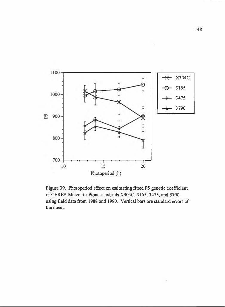
148
X304C
- 9 - 3165
3475
- A - 3790
10 15Photoperiod (h)
20
Figure 39. Photoperiod effect on estimating fitted P5 genetic coefficient of CERES-Maize for Pioneer hybrids X304C, 3165, 3475, and 3790 using field data from 1988 and 1990. Vertical bars are standard errors of the mean.
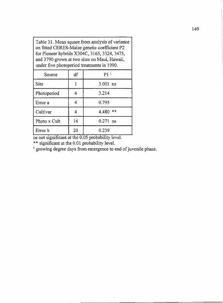
149
Table 31. Mean square from analysis of variance on fitted CERES-Maize genetic coefficient P2 for Pioneer hybrids X304C, 3165, 3324, 3475, and 3790 grown at two sites on Maui, Hawaii, under five photoperiod treatments in 1990.
Source df PI '
Site 1 3.001 ns
Photoperiod 4 3.214
Error a 4 0.795
Cultivar 4 4.480 **
Photo X Cult 16 0.271 ns
Error b 20 0.239ns not significant at the 0.05 probability level.** significant at the 0.01 probability level.' growing degree days from emergence to end of juvenile phase.
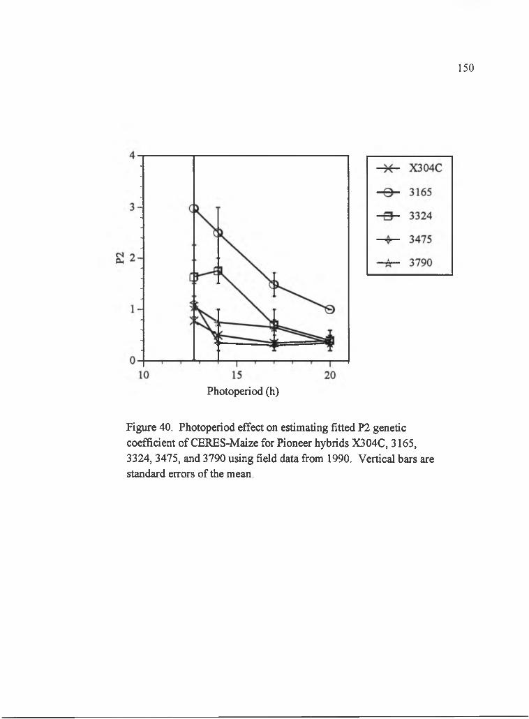
150
Photoperiod (h)
Figure 40. Photoperiod effect on estimating fitted P2 genetic coefficient of CERES-Maize for Pioneer hybrids X304C, 3165, 3324, 3475, and 3790 using field data from 1990. Vertical bars are standard errors of the mean.
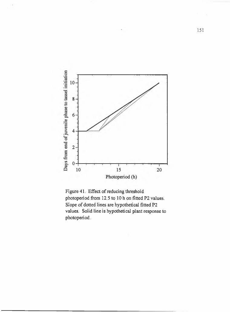
151
Figure 41. Effect of reducing threshold photoperiod from 12.5 to 10 h on fitted P2 values. Slope of dotted lines are hypothetical fitted P2 values. Solid line is hypothetical plant response to photoperiod.

value with increasing photoperiod was seen in the fitted P2 genetic coefficient (figure
40).
The fitted kernel number per plant and kernel growth rate genetic coefficients,
G2 and G2, showed photoperiod dependence for some cultivars. G2 had highly
significant cultivar and photoperiod-by-cultivar interaction sources of variation
(Table 32). Linear trend over photoperiod comparisons revealed that Pioneer hybrid
X304C was highly significantly (p>0.01) different from the other hybrids (figure 42).
Pioneer hybrid X304C had decreased number of kernels per plant as photoperiod
increased while the other hybrids had relatively stable kernel number as photoperiod
increased. The decreased kernels per plant for Pioneer hybrid X304C were probably
due to desynchronization of tassel and silk growth stages. G3 had significant cultivar
effect. There was no significant photoperiod-by-cultivar effect, but linear trends over
photoperiod indicated that Pioneer hybrid X304C was significantly different from the
others and Pioneer hybrid 3475 was different from 3790 (Table 32). Pioneer hybrid
X304C had increased G3 as photoperiod increased while G3 values for Pioneer
hybrids 3165, 3324, and 3475 decreased (figure 43). Pioneer hybrid 3790 had G3
that remained relatively stable as photoperiod increased. The relationship between
photoperiod and fitted G2 and G3 values were similar to the explicitly calculated G2
and G3 values. So, similar causes for these relationships can be assumed.
Curiously, year-by-cultivar interaction was significant for the crop coefficient
that determines the thermal time from planting to emergence, P9. Analysis of
152
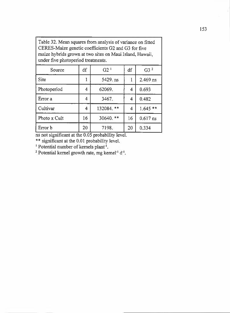
153
Table 32. Mean squares from analysis of variance on fitted CERES-Maize genetic coefficients G2 and G3 for five maize hybrids grown at two sites on Maui Island, Hawaii, under five photoperiod treatments.
Source df G 2 ' df G 3 '
Site 1 5429. ns 1 2.469 ns
Photoperiod 4 62069. 4 0.693
Error a 4 3467. 4 0.482
Cultivar 4 132084. ** 4 1.645 **
Photo X Cult 16 30640. ** 16 0.617 ns
Error b 20 7198. 20 0.334ns not significant at the 0.05 probability level. ** significant at the 0.01 probability level.' Potential number of kernels plant'.' Potential kernel growth rate, mg kernel'd ''.
154
-k- 3790
Photoperiod (h)
Figure 42. Photoperiod effect on estimating fitted G2 genetic coefficient of CERES-Maize for Pioneer hybrids X304C, 3165, 3324, 3475, and 3790 using field data from 1990. Vertical bars are standard errors of the mean.
155
- 0 - X304C
- 0 - 3165
- g - 3324
0 - 3475
-A - 3790
10 15Photoperiod (h)
20
Figure 43. Photoperiod effect on estimating fitted G3 genetic coefficient of CERES-Maize for Pioneer hybrids X304C, 3165, 3324, 3475, and 3790 using field data from 1990. Vertical bars are standard errors o f the mean.
variance showed no cultivar differences for P9, but a highly significant year-by-
cultivar interaction effect was present (Table 33). Pioneer hybrid X304C had a
constant P9 value across years while the other hybrids had lower P9 values in 1990
(figure 44). The soil-air temperature difference was almost identical for the maize
plantings in 1988 and 1990. Soil temperature was 23.6 and 22.6 °C in 1988 and 1990
which would not cause differences in emergence due to differing cold tolerance.
Hence, soil-air temperature difference and hybrid temperature tolerance cannot
account for these results.
Photoperiod affected the fitted thermal time to add a leaf primordia,
XLPGDD. XLPGDD was significantly different among cultivars (Table 34). There
was no significant photoperiod-by-cultivar interaction, but orthogonal linear trend
over photoperiods indicated that Pioneer hybrid X304C and 3324 were different
(p>0.05). Pioneer hybrid X304C had XLPGDD that decreased as photoperiod
increased while Pioneer hybrid 3324 showed a slighter decrease (figure 45).
Generally, leaf primordia seemed to initiate faster under longer photoperiod that
caused the significant linear trends.
The thermal time to fully expand one leaf, PCHRON, seemed related to
photoperiod. PCHRON had no significant sources of variation (Table 34). However,
orthogonal linear trend over photoperiods indicated that Pioneer hybrid X304C was
significantly different from Pioneer hybrids 3165, 3475, and 3790. Pioneer hybrid
X304C required more thermal time to expand a leaf as photoperiod increased, but
156
157
Table 33. Mean squares from analysis of variance on fitted CERES-Maize crop coefficient P9 for Pioneer hybrids X304C, 3165, 3475, and 3790 grown at two sites on Maui Island, Hawaii, under five photoperiod treatments.
Source df P 9 '
Year 1 1805.00 ns
Site(Year) 2 342.50
Photoperiod 4 14.38
Year X Photo 4 14.38 ns
Error 8 14.38
Cultivar 3 6.67 ns
Year X Cult 3 165.00 **
Photo X Cult 1 2 3.54 ns
Year X Photo x Cult 1 2 3.54 ns
Error 30 13.33ns not significant at the 0.05 probability level. ** significant at the 0 . 0 1 probability level.
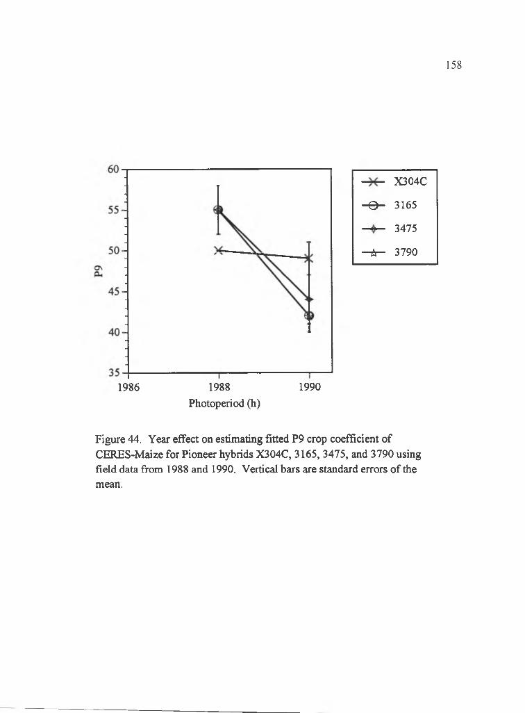
158
X304C
- 9 - 3165
3475
-A - 3790
1986 1988 Photoperiod (h)
1990
Figure 44. Year effect on estimating fitted P9 crop coefficient of CERES-Maize for Pioneer hybrids X304C, 3165, 3475, and 3790 using field data from 1988 and 1990. Vertical bars are standard errors of the mean.
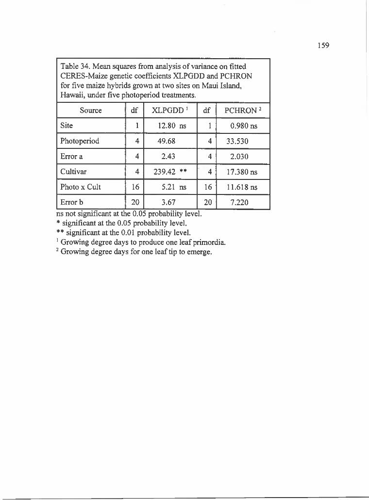
159
Table 34. Mean squares from analysis of variance on fitted CERES-Maize genetic coefficients XLPGDD and PCHRON for five maize hybrids grown at two sites on Maui Island, Hawaii, under five photoperiod treatments.
Source df XLPGDD' df PCHRON'
Site 1 12.80 ns 1 0.980 ns
Photoperiod 4 49.68 4 33.530
Error a 4 2.43 4 2.030
Cultivar 4 239.42 ** 4 17.380 ns
Photo X Cult 16 5.21 ns 16 11.618 ns
Error b 2 0 3.67 2 0 7.220ns not significant at the 0.05 probability level.* significant at the 0.05 probability level.** significant at the 0 . 0 1 probability level.' Growing degree days to produce one leaf primordia. Growing degree days for one leaf tip to emerge.
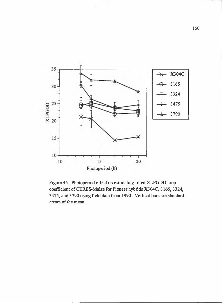
160
-0 - X304C
- 0 - 3165
-a- 3324
0 - 3475
-A - 3790
Photoperiod (h)
Figure 45. Photoperiod effect on estimating fitted XLPGDD crop coefficient of CERES-Maize for Pioneer hybrids X304C, 3165, 3324, 3475, and 3790 using field data from 1990. Vertical bars are standard errors of the mean.

Pioneer hybrids 3165, 3475, and 3790 did not (figure 46). The thermal time to
expand a leaf was related to photoperiod, but the relation was cultivar dependent.
The significant environment-by-genotype interactions for the genetic
coefficients may be attributable to errors in field data, genetic coefficient estimation
method, or model assumptions. One cause of field data error may be that the light
quality difference between artificial and sun light may have affected growth or
development. The natural photoperiod treatment had the same photoperiod length as
the control. In the natural photoperiod treatment, the artificial light extension before
sunrise and after sunset was equivalent to the civil twilight, so differences between
the natural and control may be due to different light quality not photoperiod.
The error analysis for soybean comparison between the control and natural
photoperiod treatments showed little differences for development, but growth
characteristics displayed some difference especially for weight seed"' and seeds pod"'.
Because the light quality of the artificial light may have affected development and
growth, a test comparing the control and natural photoperiod treatments was
conducted with Willmott's (1981) error analysis statistics where model predictions
were plotted against observed values. Soybean development did not seem to be
affected by light quality. The time to growth stages emergence, flowering, and
physiological maturity and the number of nodes on the mainstem were not greatly
affected when exposed to artificial lights. The time to emergence, flowering,
physiological maturity, and node number had indices of agreement of 0.94 or greater
161
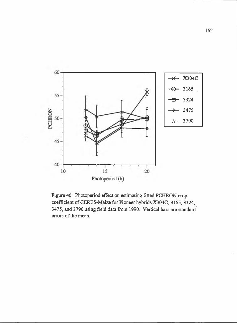
162
0 9 X304C
- 9 - 3165
- g - 3324
9 - 3475
-A - 3790
Photoperiod (h)
Figure 46. Photoperiod effect on estimating fitted PCHRON crop coefficient of CERES-Maize for Pioneer hybrids X304C, 3165, 3324, 3475, and 3790 using field data from 1990. Vertical bars are standard errors of the mean.

(Table 35). Further, for the phase durations, a greater proportion of mean square error
(MSE) was unsystematic that signified most of the variation between the two
treatments was random. Aboveground biomass, seed yield, and pod number m"’ were
strongly related despite artificial light exposure. The indices of agreement for the
three characteristics were 0.86 to 0.91 despite a relatively high mean absolute error
(Table 36). Abovegroimd biomass and pod number m ’ had high proportions of
systematic MSE that was indicative of a multiplicative bias rather than additive. Seed
yield had MSE equally partitioned between systematic and unsystematic (Table 36).
The yield components weight seed * and seeds pod * had relatively low indices of
agreement, 0.79 and 0.76 (Table 36). Both yield components had very high
proportions o f unsystematic error compared to systematic. However, the relatively
poor relation between the photoperiod treatments for weight seed * and seeds pod *
seemed to be caused by the data from the cultivar 'Bragg' at Kuiaha in 1989. When
this data point was eliminated, the indices of agreement increased from 0.79 to 0.83
and 0.76 to 0.85 for weight seed'* and seeds pod"'. So, while not firmly substantiated,
light quality in the artificially extended photoperiod treatments may have affected the
growth characteristics weight seed'* and seeds pod'*, but not biomass, seed yield, pod
number m"’ , and development.
Light quality effects on maize development and growth seemed minimal.
Error analysis between the control and natural photoperiod treatments for the
development characteristics days to tassel initiation, silking, and physiological
163
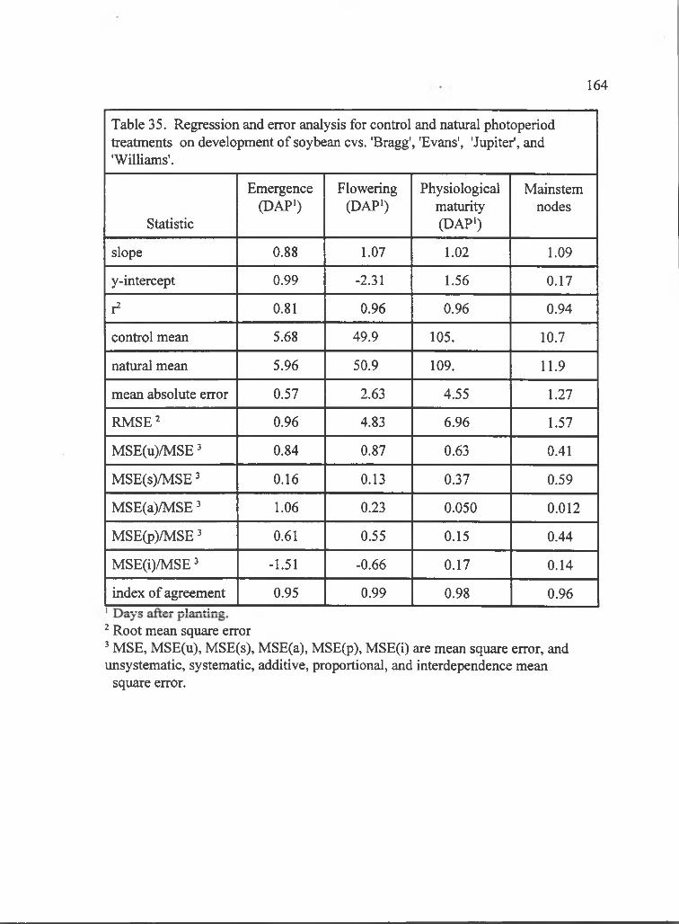
164
Table 35. Regression and error analysis for control and natural photoperiod treatments on development of soybean cvs. 'Bragg', 'Evans', 'Jupiter', and 'Williams'.
Statistic
Emergence(DAP')
Flowering(DAP')
Physiologicalmaturity(DAP')
Mainstemnodes
slope 0 . 8 8 1.07 1 . 0 2 1.09
y-intercept 0.99 -2.31 1.56 0.17
r2 0.81 0.96 0.96 0.94
control mean 5.68 49.9 105. 10.7
natural mean 5.96 50.9 109. 11.9
mean absolute error 0.57 2.63 4.55 1.27
RM SE 2 0.96 4.83 6.96 1.57
MSE(u)/MSE ^ 0.84 0.87 0.63 0.41
MSE(s)/MSE ^ 0.16 0.13 0.37 0.59
MSE(a)/MSE ^ 1.06 0.23 0.050 0 . 0 1 2
MSE(p)/MSE' 0.61 0.55 0.15 0.44
MSE(i)/MSE ^ -1.51 -0 . 6 6 0.17 0.14
index of agreement_______ _____________-.1______ 4. : - ^ 0.95 0.99 0.98 0.96
Root mean square error MSE, MSE(u), MSE(s), MSE(a), MSE(p), MSE(i) are mean square error, and
unsystematic, systematic, additive, proportional, and interdependence mean square error.
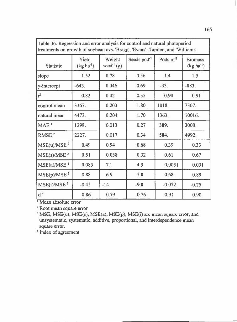
165
Table 36. Regression and error analysis for control and natural photoperiod treatments on growth of soybean cvs. 'Bragg', 'Evans', 'Jupiter', and 'Williams'.
StatisticYield
(kg ha-')Weight
seed-' (g)Seeds pod'' Pods m- Biomass
(kg ha-')
slope 1.52 0.78 0.56 1.4 1.5
y-intercept -643. 0.046 0.69 -33. -883.
0.82 0.42 0.35 0.90 0.91
control mean 3367. 0.203 1.80 1018. 7307.
natural mean 4473. 0.204 1.70 1363. 10016.
M A E' 1298. 0.013 0.27 389. 3000.
RMSE^ 2227. 0.017 0.34 584. 4992.
MSE(u)/MSE' 0.49 0.94 0 . 6 8 0.39 0.33
MSE(s)/MSE ^ 0.51 0.058 0.32 0.61 0.67
MSE(a)/MSE ^ 0.083 7.1 4.3 0.0031 0.031
MSE(p)/MSE' 0 . 8 8 6.9 5.8 0 . 6 8 0.89
MSE(i)/MSE' -0.45 -14. -9.8 -0.072 -0.25
d^ 0 . 8 6 0.79 0.76 0.91 0.90' Mean absolute error Root mean square error MSE, MSE(u), MSE(s), MSE(a), MSE(p), MSE(i) are mean square error, and unsystematic, systematic, additive, proportional, and interdependence mean square error.
* Index of agreement

maturity and total leaf number showed high agreement. The index of agreement was
0.97 to 0.99 for development attributes (Table 37). Further, the mean absolute errors
were very low compared to the means, the regression lines had slopes were nearly one
and the y-intercepts close to zero, and unsystematic mean square errors dominated
systematic for most characteristics (Table 37). Similarly, high agreement between the
two photoperiod treatments was present for maize growth attributes. The indices of
agreement for yield, kernel weight, kernels m"’ , and aboveground biomass were 0.94
to 0.98 (Table 38). The regression line slope and y-intercept, mean absolute error,
and unsystematic error were also indicated high agreement between the photoperiod
treatments. So, light quality of incandescent lamps before sunrise and after sunset did
not seem to affect maize development and growth.
Subsamples within photoperiod treatments indicated that measurement error
and within plot heterogeneity in a photoperiod treatment was small. The subsample
variance represents the accumulation of errors in measurement in the field and
laboratory, and plot heterogeneity. The subsample variance was used to estimate the
precision of the within plot cultivar means for development and growth
characteristics, i.e., the standard error. The standard error was very low in relation to
the overall range of values for days to development stages, yield, yield components,
and aboveground biomass weight (Figures 47 to 70). The small measurement errors
would not fully account for differences between observed and simulated
characteristics.
166
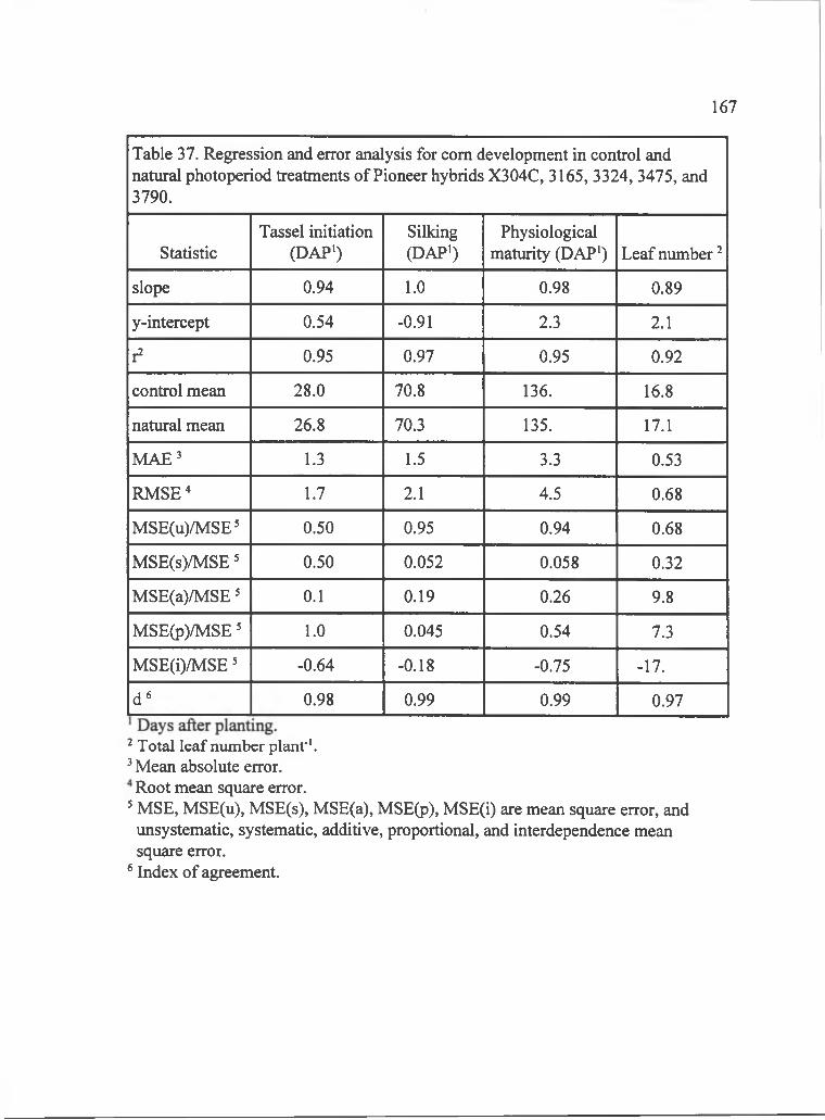
167
Table 37. Regression and error analysis for com development in control and natural photoperiod treatments of Pioneer hybrids X304C, 3165, 3324, 3475, and 3790.
StatisticTassel initiation
(DAP*)Silking(DAP*)
Physiological maturity (DAP*) Leaf num ber'
slope 0.94 1 . 0 0.98 0.89
y-intercept 0.54 -0.91 2.3 2 . 1
r 0.95 0.97 0.95 0.92
control mean 28.0 70.8 136. 16.8
natural mean 26.8 70.3 135. 17.1
M A E ' 1.3 1.5 3.3 0.53
RMSE^ 1.7 2 . 1 4.5 0 . 6 8
MSE(u)/MSE' 0.50 0.95 0.94 0 . 6 8
MSE(s)/MSE' 0.50 0.052 0.058 0.32
MSE(a)/MSE' 0 . 1 0.19 0.26 9.8
MSE(p)/MSE' 1 . 0 0.045 0.54 7.3
MSE(i)/MSE' -0.64 -0.18 -0.75 -17.
d« 0.98 0.99 0.99 0.97
' Total leaf number plant'*.' Mean absolute error.
Root mean square error.' MSE, MSE(u), MSE(s), MSE(a), MSE(p), MSE(i) are mean square error, and
unsystematic, systematic, additive, proportional, and interdependence mean square error.
* Index of agreement.
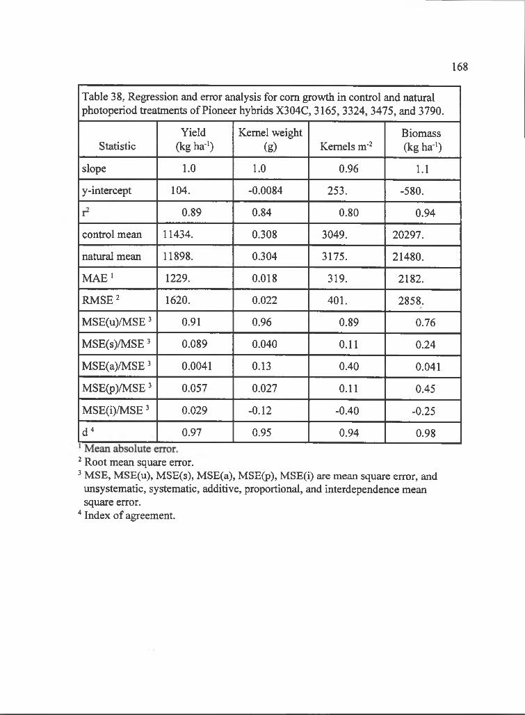
168
Table 38, Regression and error analysis for com growth in control and natural photoperiod treatments of Pioneer hybrids X304C, 3165, 3324, 3475, and 3790.
StatisticYield
(kg ha-*)Kernel weight
(g) Kernels m'^Biomass (kg ha-*)
slope 1 . 0 1 . 0 0.96 1 . 1
y-intercept 104. -0.0084 253. -580.
0.89 0.84 0.80 0.94
control mean 11434. 0.308 3049. 20297.
natural mean 11898. 0.304 3175. 21480.
MAE* 1229. 0.018 319. 2182.
R M SE' 1620. 0 . 0 2 2 401. 2858.
MSE(u)/MSE' 0.91 0.96 0.89 0.76
MSE(s)/MSE' 0.089 0.040 0 . 1 1 0.24
MSE(a)/MSE' 0.0041 0.13 0.40 0.041
MSE(p)/MSE' 0.057 0.027 0 . 1 1 0.45
MSE(i)/MSE' 0.029 -0 . 1 2 -0.40 -0.25
d^ 0.97 0.95 0.94 0.98
Root mean square error.' MSE, MSE(u), MSE(s), MSE(a), MSE(p), MSE(i) are mean square error, and
unsystematic, systematic, additive, proportional, and interdependence mean square error.
* Index of agreement.
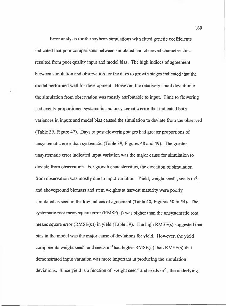
Error analysis for the soybean simulations with fitted genetic coefficients
indicated that poor comparisons between simulated and observed characteristics
resulted from poor quality input and model bias. The high indices of agreement
between simulation and observation for the days to growth stages indicated that the
model performed well for development. However, the relatively small deviation of
the simulation from observation was mostly attributable to input. Time to flowering
had evenly proportioned systematic and unsystematic error that indicated both
variances in inputs and model bias caused the simulation to deviate from the observed
(Table 39, Figure 47). Days to post-flowering stages had greater proportions of
unsystematic error than systematic (Table 39, Figures 48 and 49). The greater
unsystematic error indicated input variation was the major cause for simulation to
deviate from observation. For growth characteristics, the deviation of simulation
from observation was mostly due to input variation. Yield, weight seed ', seeds m"’,
and aboveground biomass and stem weights at harvest maturity were poorly
simulated as seen in the low indices of agreement (Table 40, Figures 50 to 54). The
systematic root mean square error (RMSE(s)) was higher than the unsystematic root
means square error (RMSE(u)) in yield (Table 39). The high RMSE(s) suggested that
bias in the model was the major cause of deviations for yield. However, the yield
components weight seed"' and seeds m'^had higher RMSE(u) than RMSE(s) that
demonstrated input variation was more important in producing the simulation
deviations. Since yield is a function of weight seed"' and seeds m ’ , the underlying
169
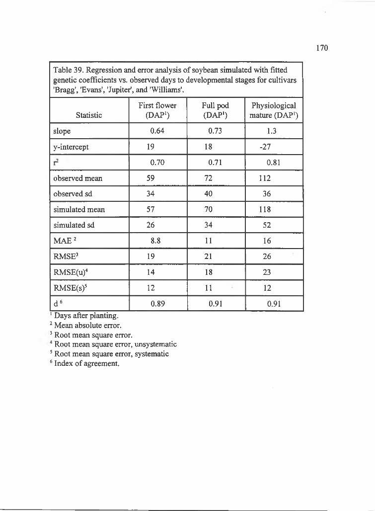
170
Table 39. Regression and error analysis of soybean simulated with fitted genetic coefficients vs. observed days to developmental stages for cultivars 'Bragg', 'Evans', 'Jupiter', and 'Williams'.
StatisticFirst flower
(DAP')Full pod (DAP')
Physiological mature (DAP')
slope 0.64 0.73 1.3
y-intercept 19 18 -27
0.70 0.71 0.81
observed mean 59 72 1 1 2
observed sd 34 40 36
simulated mean 57 70 118
simulated sd 26 34 52
MAE^ 8 . 8 1 1 16
RMSE^ 19 2 1 26
RMSECu)-* 14 18 23
RMSE(s)5 1 2 1 1 1 2
d '' 0.89 0.91 0.91' Days after planting. Mean absolute error.
3 Root mean square error.Root mean square error, unsystematic
* Root mean square error, systematic ® Index of agreement.
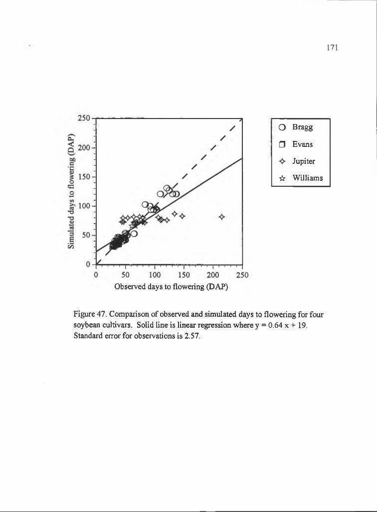
171
o Bragg
□ Evans
Jupiter
☆ Williams
Observed days to flowering (DAP)
Figure 47. Comparison of observed and simulated days to flowering for four soybean cultivars. Solid line is linear regression where y = 0.64 x + 19. Standard error for observations is 2.57.
172
o Bragg
□ Evans
Jupiter
☆ Williams
Observed days to full pod (DAP)
Figure 48. Comparison of observed and simulated days to full pod using fitted genetic coefficients for four soybean cultivars. Solid line is linear regression where y = 0.73 x + 18. Standard error for obervations is 2.42.
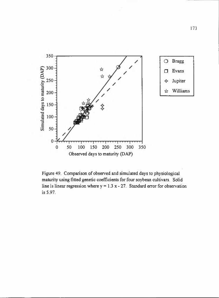
173
o Bragg
□ Evans
Jupiter
☆ Williams
Observed days to maturity (DAP)
Figure 49. Comparison of observed and simulated days to physiological maturity using fitted genetic coefficients for four soybean cultivars. Solid line is linear regression where y = 1 .3 x - 27. Standard error for observation is 5.97.
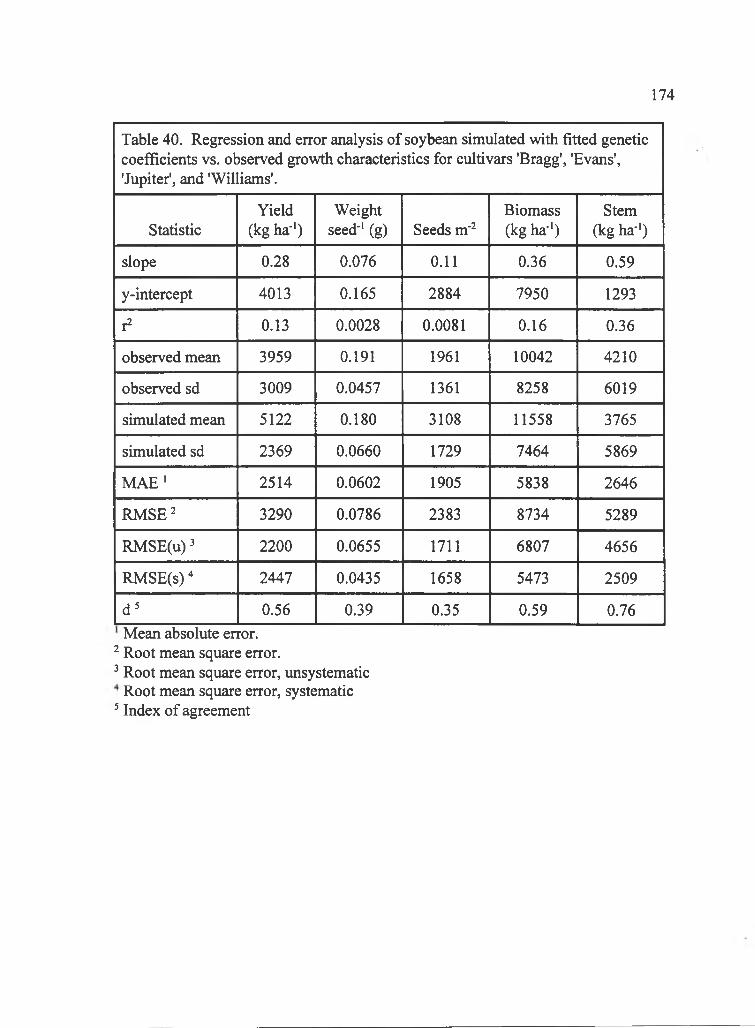
174
Table 40. Regression and error analysis of soybean simulated with fitted genetic coefficients vs. observed growth characteristics for cultivars 'Bragg', 'Evans', 'Jupiter', and 'Williams'.
StatisticYield
(kg ha-')Weight
seed-' (g) Seeds m-Biomass (kg ha-')
Stem (kg ha-')
slope 0.28 0.076 0 . 1 1 0.36 0.59
y-intercept 4013 0.165 2884 7950 1293
r2 0.13 0.0028 0.0081 0.16 0.36
observed mean 3959 0.191 1961 10042 4210
observed sd 3009 0.0457 1361 8258 6019
simulated mean 5122 0.180 3108 11558 3765
simulated sd 2369 0.0660 1729 7464 5869
M A E' 2514 0.0602 1905 5838 2646
RMSE^ 3290 0.0786 2383 8734 5289
RMSE(u) ^ 2 2 0 0 0.0655 1711 6807 4656
RMSE(s)" 2447 0.0435 1658 5473 2509
d^ 0.56 0.39 0.35 0.59 0.76Mean absolute error.
Root mean square error. Root mean square error, unsystematic Root mean square error, systematic
Index of agreement
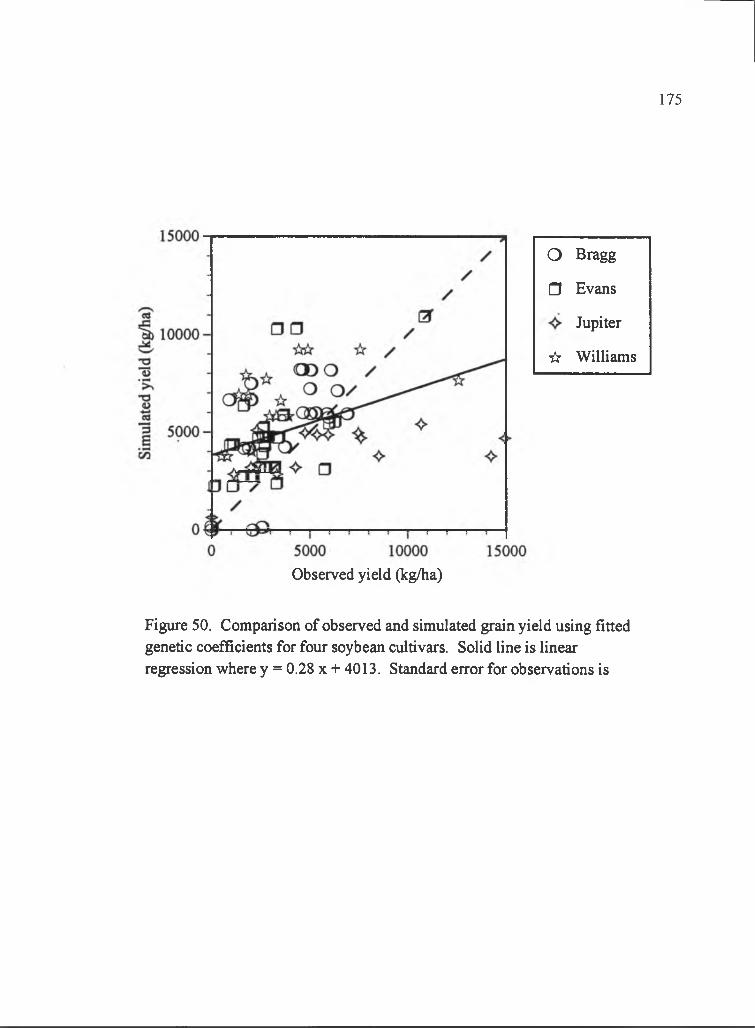
175
o Bragg
□ Evans
Jupiter
☆ Williams
Observed yield (kg/ha)
Figure 50. Comparison of observed and simulated grain yield using fitted genetic coefficients for four soybean cuitivars. Solid line is linear regression where y = 0.28 x + 4013. Standard error for observations is
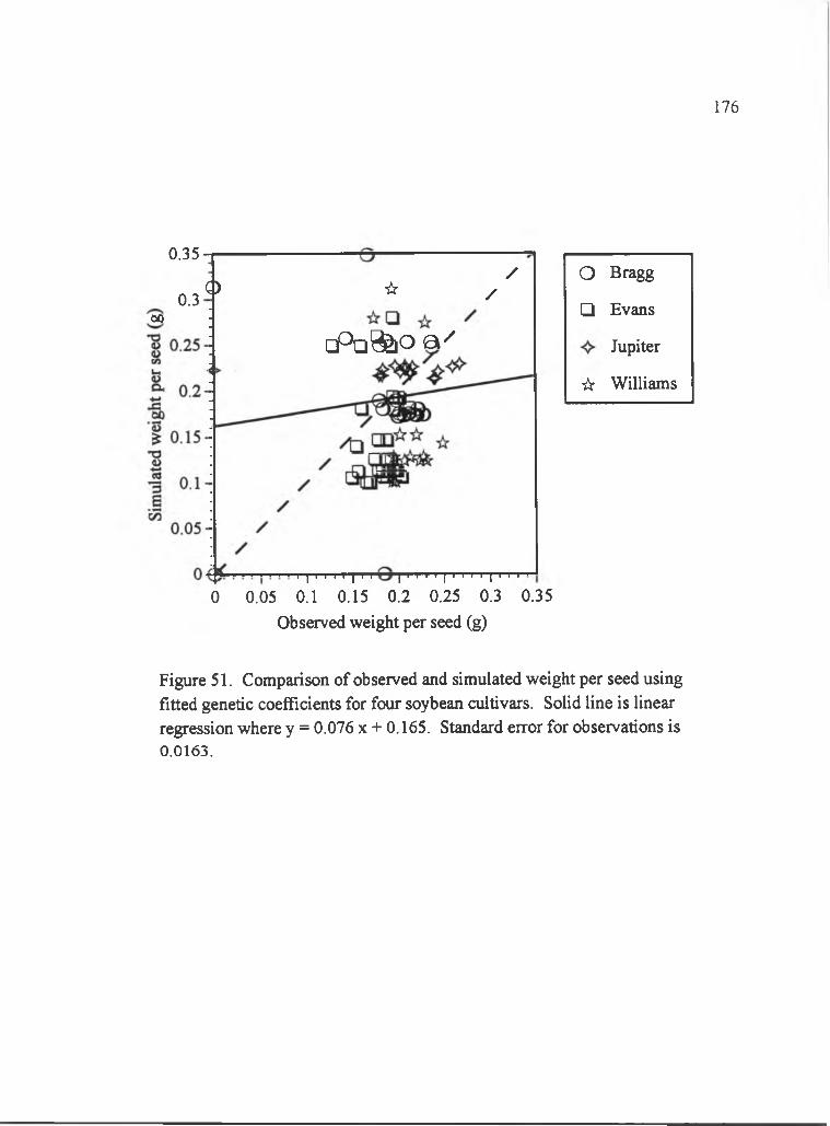
176
0.35
0 .3 *00
☆ /
□ P o Q i i o a ' '
/
I I I I I I I I I I I I I I I I I I I I I I I
0 0.05 0.1 0.15 0.2 0.25 0.3 0.35Observed weight per seed (g)
o Bragg
□ Evans
Jupiter
☆ Williams
Figure 51. Comparison of observed and simulated weight per seed using fitted genetic coefficients for four soybean cultivars. Solid line is linear regression where y = 0.076 x + 0.165. Standard error for observations is 0.0163.
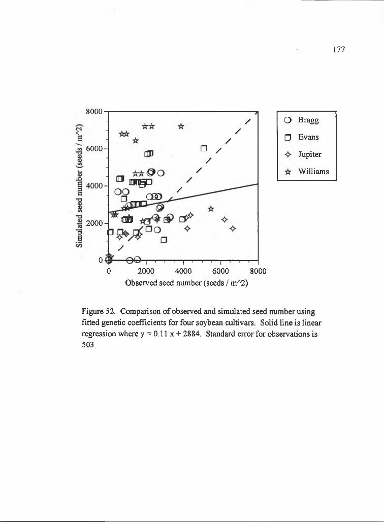
8000'
a6000
u
2000-
I
//
a / /
/
/m s^
_ o o o ^
0 ^
(nil
/I Q O I I I I I I I
0 2000 4000 6000 8000Observed seed number (seeds / m ' 2)
177
o Bragg
□ Evans
Jupiter
Williams
Figure 52. Comparison of observed and simulated seed number using fitted genetic coefficients for four soybean cultivars. Solid line is linear regression where y = 0.11 x + 2884. Standard error for observations is 503.
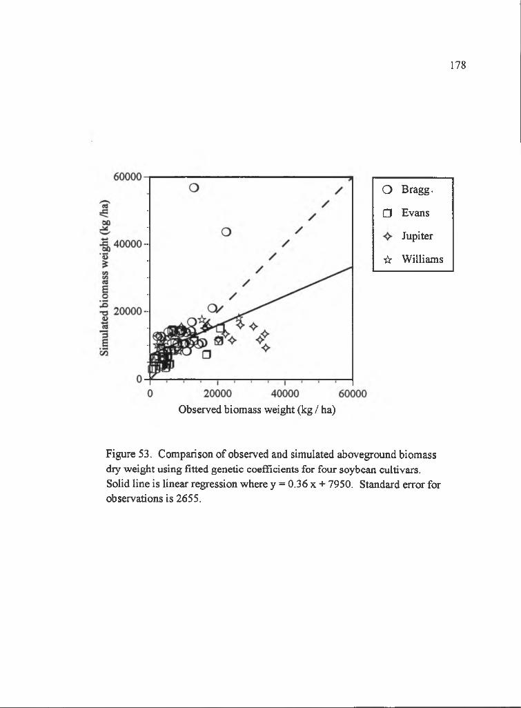
178
o Bragg.
□ Evans
Jupiter
☆ Williams
Observed biomass weight (kg / ha)
Figure 53. Comparison of observed and simulated aboveground biomass dry weight using fitted genetic coefficients for four soybean cultivars. Solid line is linear regression where y = 0.36 x + 7950. Standard error for observations is 2655.
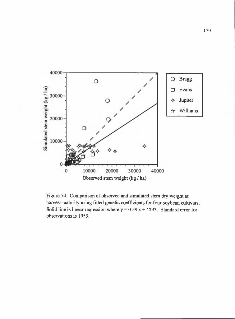
179
o Bragg
□ Evans
Jupiter
☆ Williams
Observed stem weight (kg / ha)
Figure 54. Comparison of observed and simulated stem dry weight at harvest maturity using fitted genetic coefficients for four soybean cultivars. Solid line is linear regression where y = 0.59 x + 1293. Standard error for observations is 1953.

error for yield may be considered unsystematic, too. Simulated aboveground biomass
and stem weights deviated from observed weights and were more attributable to
input variation. Input variation, more than model bias, may be responsible for
deviations since RMSE(u) was greater than RMSE(s) (Table 40). While the deviation
o f simulated soybean development and growth from observations resulted from input
variation and model bias, input variation was the greater cause.
Maize simulations showed that model bias produced deviations from observed
development and growth more than input variations. Regardless of the genetic
coefficient determination method, RMSE(s) was generally greater than or equal to
RMSE(u) for days to development stages (Tables 41 and 42, Figures 55 to 57 and 58
to 60). The greater RMSE(s) suggested that model bias was the greater cause for
simulation deviation from observation. Similarly, the growth characteristics yield,
yield components, above ground biomass and stover weights at harvest maturity had
higher RMSE(s) than RMSE(u) regardless of genetic coefficient determination
method (Tables 43 and 44, Figures 61 to 65 and 6 6 to 70). The high RMSE(s)
suggested that model bias was the major contributor to the growth simulation
deviation from observation for maize. Hence, the error in simulated development and
growth resulted mostly from model bias, but uncertainty in the input parameters also
contributed to the error.
Error analysis for maize simulation vs. observation demonstrated that fitted
genetic coefficients, including leaf number modifications, could correct some model
180
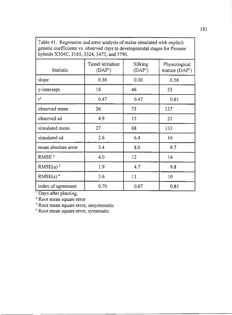
181
Table 41. Regression and error analysis of maize simulated with explicit genetic coefficients vs. observed days to developmental stages for Pioneer hybrids X304C, 3165, 3324, 3475, and 3790.
StatisticTassel initiation
(DAP')Silking(DAP')
Physiological mature (DAP')
slope 0.36 0.30 0.58
y-intercept 18 46 53
r 0.47 0.47 0.61
observed mean 26 73 137
observed sd 4.9 15 2 1
simulated mean 27 6 8 133
simulated sd 2 . 6 6.4 16
mean absolute error 3.4 8 . 0 9.7
RMSE^ 4.0 1 2 14
RM SE(u)' 1.9 4.7 9.8
RMSE(s) ^ 3.6 1 1 1 0
index of agreement 0.70 0.67 0.85Days after planting.
Root mean square error ' Root mean square error, unsystematic
Root mean square error, systematic
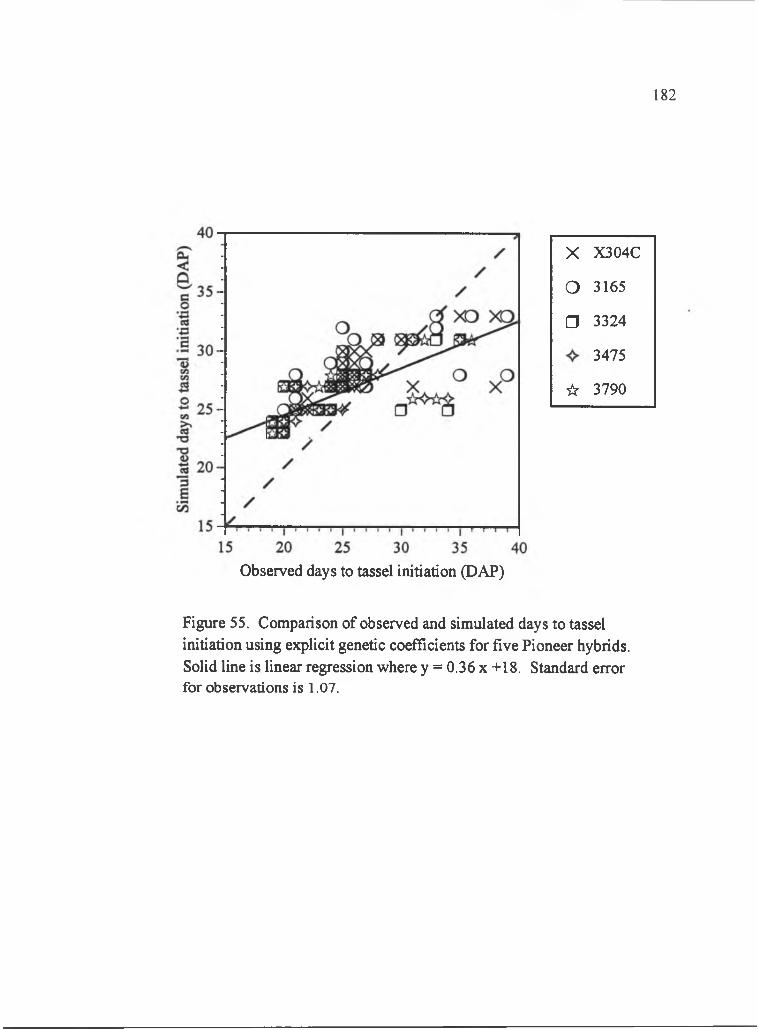
182
X X304C
o 3165
□ 3324
3475
☆ 3790
Observed days to tassel initiation (DAP)
Figure 55. Comparison of observed and simulated days to tassel initiation using explicit genetic coefficients for five Pioneer hybrids. Solid line is linear regression where y = 0.36 x +18. Standard error for observations is 1.07.
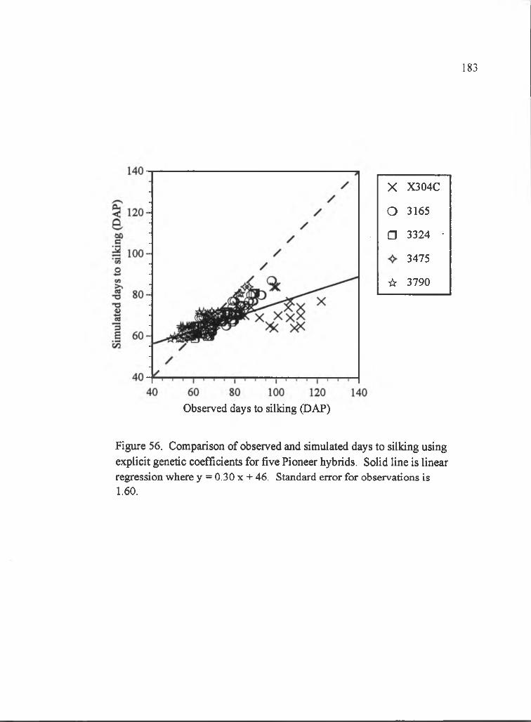
183
X X304C
o 3165
□ 3324 •
3475
☆ 3790
Observed days to silking (DAP)
Figure 56. Comparison of observed and simulated days to silking using explicit genetic coefficients for five Pioneer hybrids. Solid line is linear regression where y = 0.30 x + 46. Standard error for observations is 1.60.
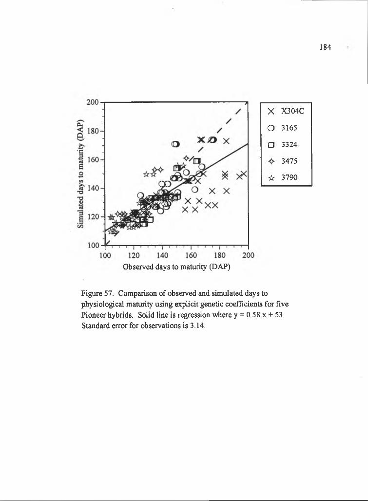
184
X X304C
o 3165
□ 3324
3475
☆ 3790
Observed days to maturity (DAP)
Figure 57. Comparison of observed and simulated days to physiological maturity using explicit genetic coefficients for five Pioneer hybrids. Solid line is regression where y = 0.58 x + 53. Standard error for observations is 3.14.
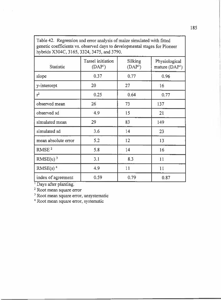
185
Table 42. Regression and error analysis of maize simulated with fitted genetic coefficients vs. observed days to developmental stages for Pioneer hybrids X304C, 3165, 3324, 3475, and 3790.
StatisticTassel initiation
(DAP')Silking(DAP‘)
Physiological mature (DAP')
slope 0.37 0.77 0.96
y-intercept 2 0 27 16
r2 0.25 0.64 0.77
observed mean 26 73 137
observed sd 4.9 15 2 1
simulated mean 29 83 149
simulated sd 3.6 14 23
mean absolute error 5.2 1 2 13
RM SE’ 5.8 14 16
RMSE(u) ’ 3.1 8.3 1 1
RMSE(s) 4.9 1 1 1 1
index of agreement 0.59 0.79 0.87Days after planting.
’ Root mean square error ’ Root mean square error, unsystematic “* Root mean square error, systematic
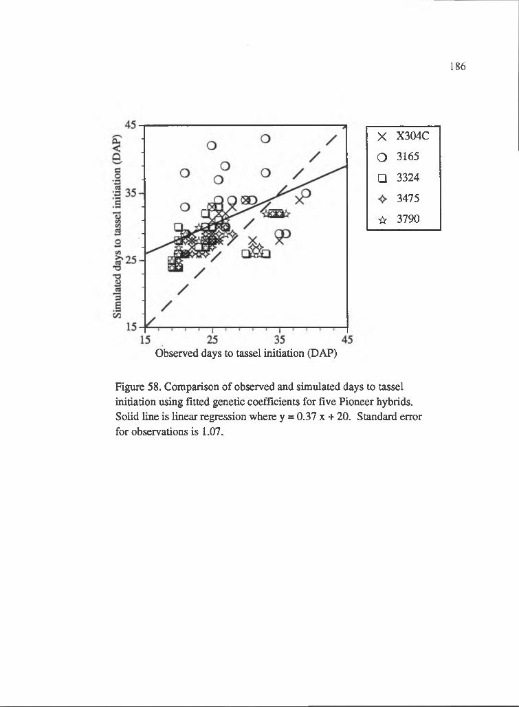
186
X X304C
o 3165
□ 3324
3475
☆ 3790
Observed days to tassel initiation (DAP)
Figure 58. Comparison of observed and simulated days to tassel initiation using fitted genetic coefficients for five Pioneer hybrids. Solid line is linear regression where y = 0.37 x + 20. Standard error for observations is 1.07.
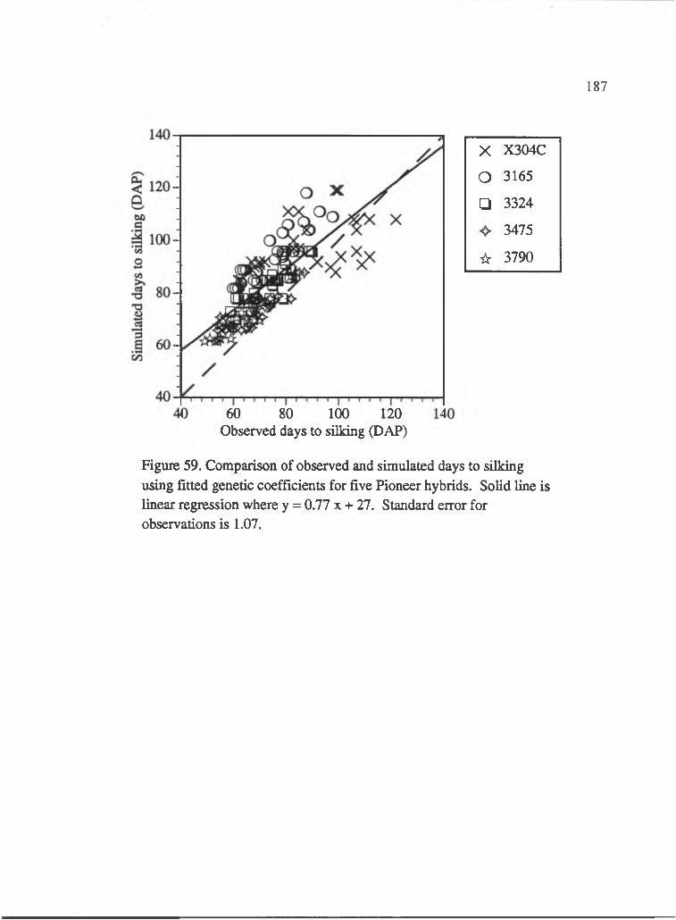
187
X X304C
o 3165
□ 3324
3475
☆ 3790
60 80 1 0 0 1 2 0
Observed days to silking (DAP)
Figure 59, Comparison of observed and simulated days to silking using fitted genetic coefficients for five Pioneer hybrids. Solid line is linear regression where y = 0.77 x + 27. Standard error for observations is 1.07,
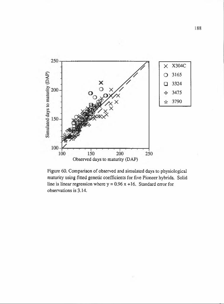
188
X X304C
o 3165
□ 3324
3475
☆ 3790
Observed days to maturity (DAP)
Figure 60. Comparison of observed and simulated days to physiological maturity using fitted genetic coefficients for five Pioneer hybrids. Solid line is linear regression where y = 0.96 x +16. Standard error for observations is 3.14.
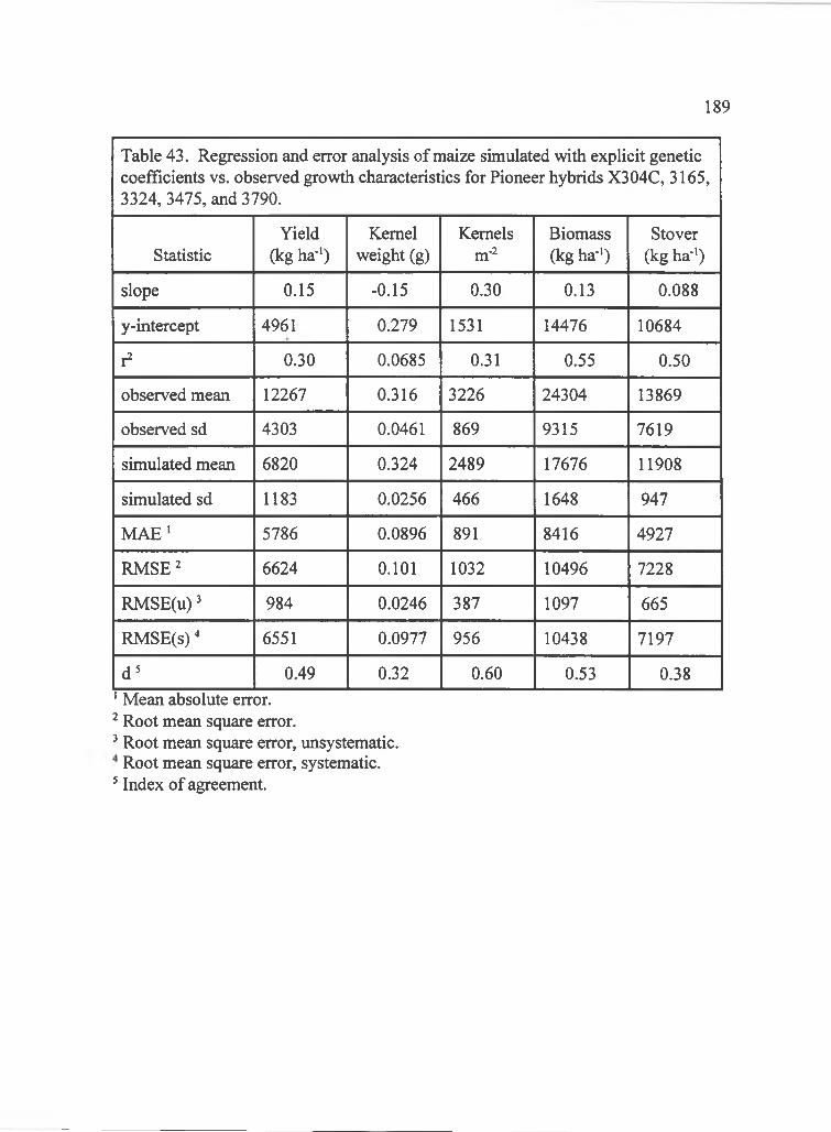
189
Table 43. Regression and error analysis of maize simulated with explicit genetic coefficients vs. observed growth characteristics for Pioneer hybrids X304C, 3165, 3324, 3475, and 3790.
StatisticYield
(kg ha-')Kernel
weight (g)Kernels
m'^Biomass (kg ha-')
Stover (kg ha-')
slope 0.15 -0.15 0.30 0.13 0.088
y-intercept 4961 0.279 1531 14476 10684
r 0.30 0.0685 0.31 0.55 0.50
observed mean 12267 0.316 3226 24304 13869
observed sd 4303 0.0461 869 9315 7619
simulated mean 6820 0.324 2489 17676 11908
simulated sd 1183 0.0256 466 1648 947
M A E' 5786 0.0896 891 8416 4927
RMSE^ 6624 0 . 1 0 1 1032 10496 7228
RMSE(u)' 984 0.0246 387 1097 665
RMSE(s) ^ 6551 0.0977 956 10438 7197
d^ 0.49 0.32 0.60 0.53 0.38' Mean absolute error. Root mean square error. Root mean square error, unsystematic.Root mean square error, systematic.
Index of agreement.
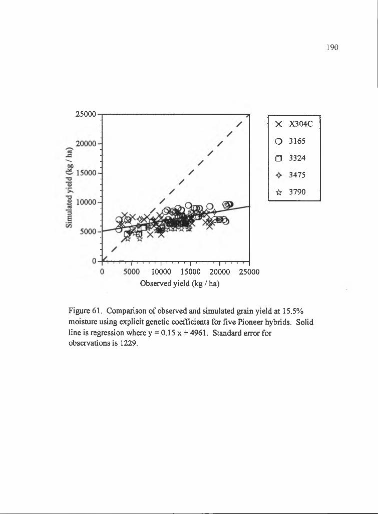
190
25000X X304C
o 3165
□ 3324
3475
☆ 3790
I ' ' ' ' I ' ' ' ' I
10000 15000 20000 25000Observed yield (kg / ha)
Figure 61. Comparison of observed and simulated grain yield at 15.5% moisture using explicit genetic coefficients for five Pioneer hybrids. Solid line is regression where y = 0.15 x + 4961. Standard error for observations is 1229.
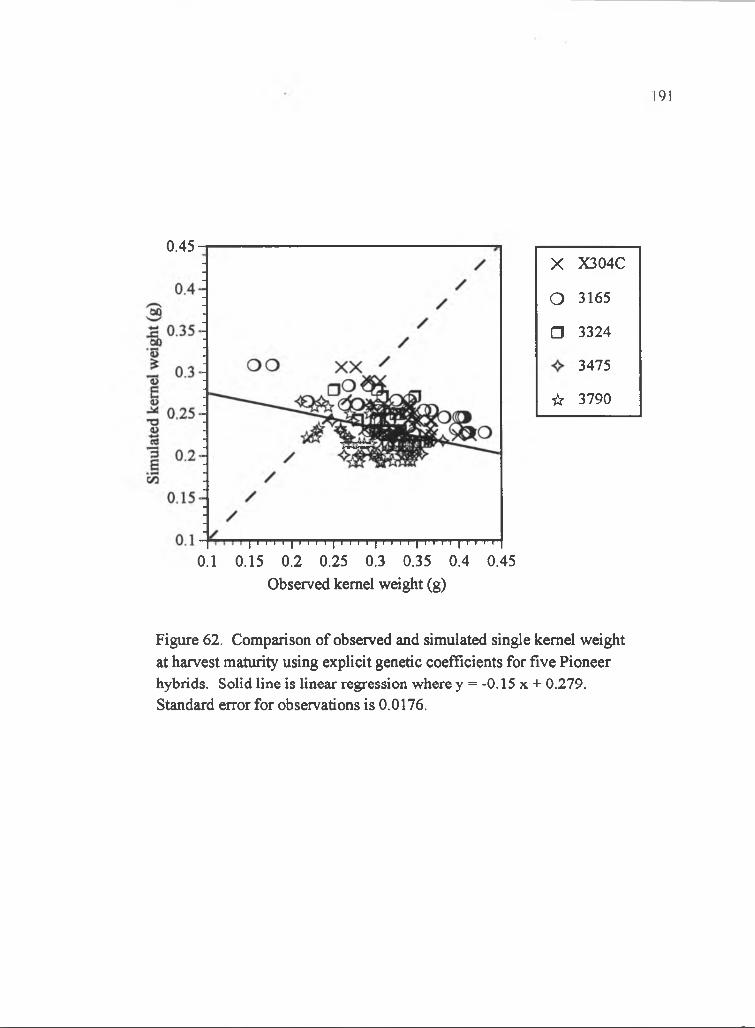
191
0.45
I I I I I I I I I I I I I I I I ' I T I I I I I I I I I I I I
0.1 0.15 0.2 0.25 0.3 0.35 0.4 0.45Observed kernel weight (g)
X X304C
o 3165
□ 3324
3475
☆ 3790
Figure 62. Comparison of observed and simulated single kernel weight at harvest maturity using explicit genetic coefficients for five Pioneer hybrids. Solid line is linear regression where y = -0.15 x + 0.279. Standard error for observations is 0.0176.
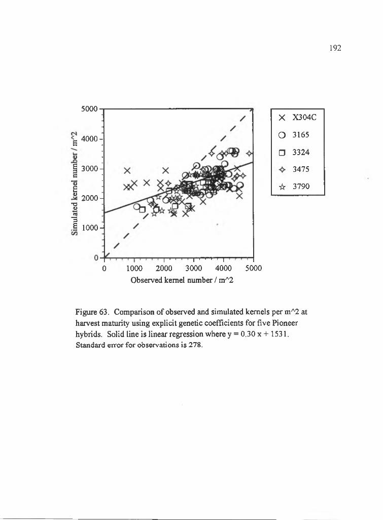
192
5000
a
Va3a"vg’T3I3a
4000-
3000-
2000 -
3 1000 -
I I I I I [ I I I I I
0 1000 2000 3000 4000 5000Observed kernel number / m^2
X X304C
o 3165
□ 3324
3475
☆ 3790
Figure 63. Comparison of observed and simulated kernels per m^2 at harvest maturity using explicit genetic coefficients for five Pioneer hybrids. Solid line is linear regression where y = 0.30 x + 1531. Standard error for observations is 278.

193
60000X X304C
o 3165
□ 3324
3475
☆ 3790
20000 40000 60000Observed biomass weight (kg / ha)
Figure 64. Comparison of observed and simulated aboveground biomass dry weight at harvest maturity using explicit genetic coefficients for five Pioneer hybrids. Solid line is linear regression where y = 0.13 x + 14476. Standard error for observations is 2493.

194
50000
I■4~*ja00
I
40000-
2P 30000-
o>
I13BK
20000 -
10000
I I I I I I I I I I I0 10000 20000 30000 40000 50000
Observed stover weight (kg / ha)
X X304C
o 3165
□ 3324
3475
☆ 3790
Figure 65. Comparison of observed and simulated stover dry weight at harvest maturity using explicit genetic coefficients for five Pioneer hybrids. Solid line is linear regression where y = 0.088 x + 10684. Standard error for observations is 1805.
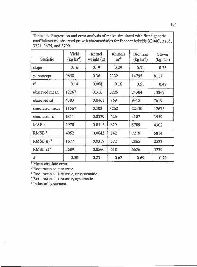
195
Table 44. Regression and error analysis of maize simulated with fitted genetic coefficients vs. observed growth characteristics for Pioneer hybrids X304C, 3165, 3324, 3475, and 3790.
StatisticYield
(kg ha-')Kernel
weight (g)Kernels
m-Biomass (kg ha-')
Stover (kg ha-')
slope 0.16 -0.19 0.29 0.31 0.33
y-intercept 9658 0.36 2332 14795 8117
r 0.14 0.068 0.16 0.51 0.49
observed mean 12267 0.316 3226 24304 13869
observed sd 4303 0.0461 869 9315 7619
simulated mean 11567 0.303 3262 22450 12673
simulated sd 1811 0.0329 626 4107 3559
M A E' 2970 0.0515 629 5789 4302
RM SE 2 4052 0.0643 842 7219 5814
RMSE(u) ^ 1677 0.0317 572 2865 2523
RMSE(s) ^ 3689 0.0560 618 6626 5239
d ' 0.50 0.23 0.62 0.69 0.70Mean absolute error.
Root mean square error. Root mean square error, unsystematic.
“ Root mean square error, systematic. Index of agreement.

196
25000
20000 -
ed
12uTD
3
c/3
15000^
10000 -
5000-
' ' ' I ' ' ' ■ I ' ' ' ' I ' ' ' ' I0 5000 10000 15000 20000 25000
Observed yield (kg/ha)
X X304C
o 3165
□ 3324
3475
☆ 3790
Figure 6 6 . Comparison of observed and simulated yield at 15.5% mositure using fitted genetic coefficients for five Pioneer hybrids. Solid line is linear regression where y = 0.16 x + 9658. Standard error for observations is 1229.
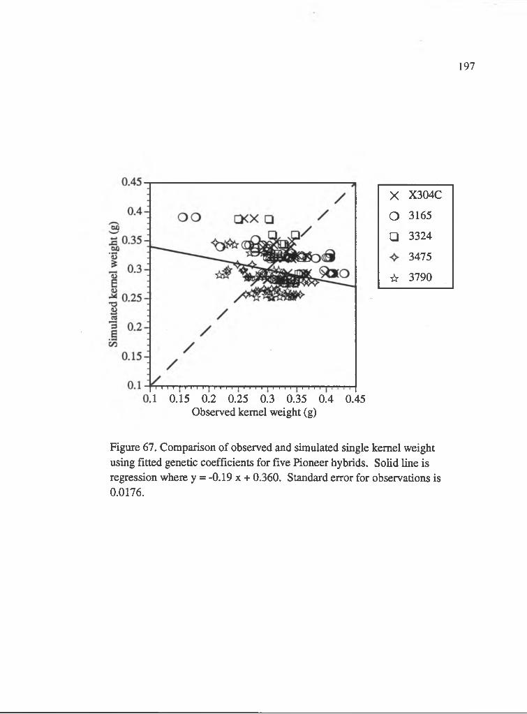
197
X X304C
o 3165
□ 3324
3475
☆ 3790
.1 0.15 0.2 0.25 0.3 0.35 0.4 0.45 Observed kernel weight (g)
Figure 67. Comparison of observed and simulated single kernel weight using fitted genetic coefficients for five Pioneer hybrids. Solid line is regression where y = -0.19 x + 0.360. Standard error for observations is 0.0176.

198
5000X X304C
o 3165
□ 3324
3475
☆ 3790
1000 2000 3000 4 ^ 5000Observed kernel number / m 2
Figure 6 8 . Comparison of observed and simulated kernel number per m'^2 at harvest maturity using fitted genetic coefficients for five Pioneer hybrids. Solid line is linear regression where y = 0.29 x + 2332. Standard error for observations is 278.

199
60000
I•1^40000-
IaoIS
20000 -
3
c/3
20000 40000 60000
X X304C
o 3165
□ 3324
3475
☆ 3790
Observed biomass weight (kg/ha)
Figure 69. Comparison of observed and simulated aboveground biomass weight at harvest maturity using fitted genetic coefficients for five Pioneer hybrids. Solid line is linear regression where y = 0.31 x + 14795.Standard error for observations is 2493.
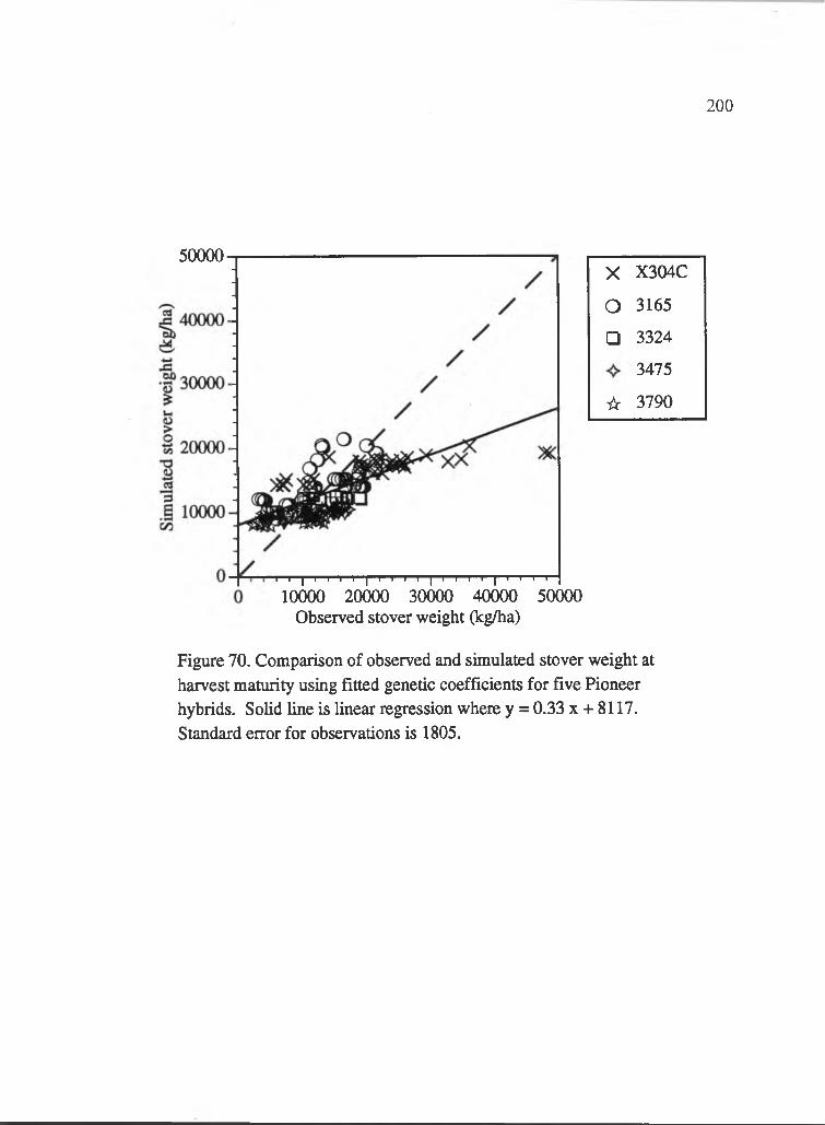
200
50000X X304C
o 3165
□ 3324
3475
☆ 3790
I I I I I I I I I I I I I I I ■ T I I I I I I
10000 20000 30000 40000 50000 Observed stover weight O^g/ha)
Figure 70. Comparison of observed and simulated stover weight at harvest maturity using fitted genetic coefficients for five Pioneer hybrids. Solid line is linear regression where y = 0.33 x + 8117. Standard error for observations is 1805.

bias for development and characteristics. Generally, the fitted genetic coefficients
and leaf number modifications gave simulations that fit the observed data better than
explicit. One exception to this generalization was the days to tassel initiation which
was better simulated when explicit genetic coefficients, rather than fitted, genetic
coefficients were used (Tables 41 and 44, Figures 55 and 58). The over-estimate of
days to tassel initiation for fitted genetic coefficients may be attributed to the
determination method. Since P2 is the slope of the regression line of days to tassel
initiation on photoperiod, in fitting the P2 genetic coefficient so that simulated tassel
initiation date matched the observed, the regression line was forced through the point
at 4 days and 12.5 h. However, the explicitly determined P2 was not forced through
any point, so fitted P2 was generally higher than explicit P2. The result o f the higher
fitted P2 was over estimating tassel initiation, hence lower index of agreement than
explicit. The indices of agreement for days to silking and maturity were slightly
higher for the fitted than explicit genetic coefficients despite having higher root mean
square error (Tables 41 and 44). Furthermore, the fitted genetic coefficients gave a
slope closer to unity and y-intercept nearer zero than explicit so the proportion of
RMSE(s) was smaller, but RMSE and mean absolute error (MAE) were larger. The
smaller proportions of RMSE(s) for days to tassel initiation and silking, the slopes
nearer unity and y-intercept nearer zero for days to silking and maturity indicated a
lesser model bias when fitted genetic coefficients and leaf modifications were used.
201

The growth characteristics yield and yield components were not substantially
affected when fitted genetic coefficients and leaf modifications were used while
stover weight was. The regression of simulated yield and yield components on
observed showed little differences in slope between fitted and explicit genetic
coefficients (Tables 43 and 44). Fitted genetic coefficients reduced the RMSE and
the proportion of RMSE(s), and increased the overall mean simulated yield and its
components when compared to the explicit genetic coefficients. The null effect on
regression slope and increased overall mean suggested that fitted genetic coefficients
increased additively increased y-intercept of the linear regression for these growth
characteristics. The result of the increased y-intercept was to reduce the RMSE(s)
with a concomitant increase in RMSE(u). So, fitting genetic coefficients was able to
increase the model response, i.e., y-intercept, to the environmental conditions in the
field experiment, but some other model component must be changed to increase the
model response, i.e., slope, to these same environmental factors. Stover weight, and
consequently aboveground biomass, showed that fitted genetic coefficients and leaf
modifications were able to decrease model bias. The regression line of simulated
stover weight on observed had increased slope when fitted genetic coefficients and
leaf modifications were used compared to explicit (Tables 43 and 44, Figures 65 and
70). Furthermore, the fitted genetic coefficients when compared to explicit genetic
coefficients brought the y-intercept closer to zero, decreased RMSE, decreased the
proportion of RMSE(s), and increased the overall simulated mean. So, the fitted
202

genetic coefficients affected the model results more for stover weight than yield and
its components, but further corrections were still necessary for all growth
characteristics.
Discussion
A major question, as yet unresolved, is whether incandescent light quality and
constant photoperiod are similar to naturally occurring conditions for soybean and
maize development and growth. Incandescent light quality may be similar to natural
light quality in its effect on soybean development. Delayed development was
observed imder long photoperiods of incandescent or natural light quality when the
genes E3 and E4 were present (Saindon, et al., 1989a; Saindon, et al., 1989b).
However, the three other loci that control development response to photoperiod have
not been determined to cause similar effects under incandescent and natural light
quality. Development rate in soybean was different under constant or shortening
photoperiod depending on stage of development (McBlain et al., 1987). In time to
flowering for soybean, the alleles E„ Ej, and E3 delayed flowering regardless of
constant or shortening photoperiods. However, in time from flowering to maturity,
the gene E, slightly delayed maturity under constant photoperiod and hastened
maturity under shortening photoperiod while gene E3 delayed maturity under constant
photoperiod and slightly delayed maturity under shortening photoperiod. The effect
of light quality and changing photoperiod on maize growth and development is not
203

well understood. While this experiment did not detect any effect of light quality on
growth and development of soybean and maize, the effect of constant photoperiod has
not been determined.
In CERES-Maize, fitting genetic coefficients seemed to correct some model
bias. There was less bias in the observed vs. simulated plots for maize development
and growth when fitted genetic coefficients were used compared to explicit. The
genetic coefficients seemed to have the ability to compensate for over- or under
response of the model's growth and development to the environment, or be able to
compensate for bias in the input parameters. This compensating effect may make the
model only suited to simulate crop development and growth under similar
environmental conditions. Hence, the assertion that fitted genetic coefficients made
CERES-Maize only applicable to the locations where the genetic coefficients were
determined (Hodges et al., 1987; Liu et al., 1989) may be caused by genetic
coefficients that uniquely adjusted crop growth and development to the environment
where they were fitted.
Genetic coefficients for crop models SOYGRO and CERES-Maize can be
determined with a fitting method, but the application of these models must be
restricted. The fitted development genetic coefficients from both models displayed
linear trends that depended on the environment where they were estimated. This
indicates that the models caimot use the fitted genetic coefficients estimated in one
environment to simulate development in a different environment. Instead, the fitted
204

genetic coefficients should be used to simulate development in an environment
similar to the one where the coefficients were estimated. Fitted growth genetic
coefficients exhibited trends over the environments from which they were estimated.
Again, this indicates that simulations with fitted genetic coefficients would be
accurate only under environments similar in which the coefficients were estimated.
So, the application of the fitted growth genetic coefficients must be restricted to the
environments where they were determined.
Explicit determination of genetic coefficients for CERES-Maize was not an
acceptable method. The simulated vs. observed comparisons showed that biases
occurred for development and growth characteristics. These biases were indicative of
problems within the model. When genetic coefficients were determined apart from
the model, the model imperfections will result in biased simulations. The simulation
bias was generally over-estimating development time and under-estimating growth
under the present experimental conditions. So, genetic coefficients and its
determination cannot be considered separately from the whole-model predictions.
One of the major problems with SOYGRO and CERES-Maize seemed to be
their inability to well simulate the components of yield. In soybean, pods plant '
response to photoperiod and temperature depended on genotype. Apparently, as
temperature increased, pods plant"' can increase under short photoperiod and
decrease in long photoperiod (Raper and Thomas, 1978), or decrease under short
photoperiod and increase in long photoperiod (Huxley et al., 1976; Saito, 1961;
205

Hesketh et al, 1973). The difference in response to temperature and photoperiod may
be related to differences in genotype (van Schaik and Probst, 1958). The complexity
o f the pods p lant' response to photoperiod may not be adequately addressed in
SOYGRO which assumes that only pod abortion occurs as photoperiod increases. In
maize, photoperiod may reduce kernel number by increasing the tassel-silk interval so
that pollination is incomplete. Pioneer hybrid X304C had increased tassel-silk
interval as photoperiod increased that resulted in lesser kernels plant'. However,
CERES-Maize does not account for decreased kernel number due to delayed silking.
In CERES-Maize, kernel number is mainly dependent on photosynthetic rate prior to
silking (Jones et al., 1986). So, under certain conditions of long photoperiod,
SOYGRO and CERES-Maize may not be able to well simulate yield components
and, consequently, yield.
Genetic coefficients for SOYGRO and CERES-Maize are environment
dependent under the present experimental conditions. The cause o f the environment
dependency may be related to model mis-specification or input parameter bias.
Whether changes in the model mechanisms, philosophy, or input parameters can
overcome the deficiency in estimating genetic coefficients are not well understood at
this time.
206

CHAPTER 4
SENSITIVITY ANALYSIS OF DERIVED GENETIC COEFFICIENTS FOR SOYGRO AND CERES-MAIZE
Introduction
Results shown in Chapter 3 indicate that SOYGRO and CERES-Maize crop
models did not accurately simulate growth and yield of soybean and maize under a
range of environments and photoperiods. Fitted genetic coefficients displayed linear
trends on photoperiod. The trends indicated that the genetic coefficients were
compensating for over- or under-predicting crop response to the environment.
Furthermore, error analysis suggested that model bias accounted for part o f the poor
match. However, specific model routines that caused the poor growth simulation
were not readily identified.
Fitted genetic coefficients for SOYGRO and CERES-Maize displayed
significant cultivar-by-photoperiod effects. The CERES-Maize genetic coefficients
P2, P5, G2, and G3 and leaf production coefficients XLPGDD and PCHRON had
significant cultivar-by- photoperiod interaction effect. SOYGRO genetic coefficients
PHTHRS 6 to 9 and SDPDVR also showed significant cultivar-by-photoperiod
interaction. The significant interaction indicated that the genetic coefficients had
different linear relations to photoperiod among varieties. The instability o f the fitted
genetic coefficients suggested that the routines in the model associated with these
genetic coefficients were possible sources of the model bias.
207

To prioritize further work on the model, the routines that have the greatest
effect on biasing the simulation results must be identified. Each fitted genetic
coefficient mean has an associated error that can be quantified by the standard error.
A genetic coefficient may have a large standard error, but if the model is insensitive
to that parameter, the variation in simulation results attributed to the input error
would be relatively small and unimportant. Therefore, the magnitude of the standard
error alone cannot indicate the importance of the genetic coefficient to prioritize
further work since the model sensitivity to that coefficient is unknown.
The objective of this experiment was to determine'which genetic coefficients,
and presumably their associated routines, are important in causing model bias.
Methods and Materials
The SOYGRO and CERES-Maize genetic coefficient means and standard
errors were obtained from a previously described fitting procedure. A field
experiment was conducted with four soybean cuitivars ('Bragg', 'Evans', 'Jupiter', and
'Williams') and five maize hybrids (Pioneer hybrids X304C, 3165, 3324, 3475, and
3790) over four planting dates. The soybean and maize were planted at two sites on
Maui Island, Hawaii, elevation 282 and 640 m, where natural photoperiod was
extended to natural + 0.5-, 14-, 17-, and 20-h with quartz lamps. Data collected
included yield and yield components, plant dry weight, and dates of growth stages.
Model inputs were produced to duplicate field weather, soil, and management
208

conditions in each photoperiod treatment at each site for each year. The models were
iteratively run with adjustments to the genetic coefficients until the model output on
yield, yield components, plant dry weight, and growth stage dates were within 1 % of
the observed field data. For maize, three other coefficients besides the genetic
coefficients were concurrently fitted. The arithmetic means and standard errors of the
fitted genetic coefficients were calculated over the photoperiod treatment, site, and
year combinations.
Sixteen SOYGRO genetic coefficients were selected to undergo sensitivity
analysis. For the following reasons, seven genetic coefficients were not included in
the analysis: VARDH, PHTHRS(l), PHTHRS(2), PHTHRS(3), PHTHRS(5), and
FLWMAX. By definition, VARDH must be set to 1.0 (Jones et al., 1986) and
PHTHRS(5) was earlier redefined as 6.20 (Thomas and Raper, 1983). The standard
errors for PHTHRS(l) and PHTHRS(2) were very small. PHTHRS(3) values were
not determined and so no associated variation was estimated. FLWMAX was not
considered important as a genetic coefficient (Jones et al., 1989), and was simply set
to two times PODVAR. The remaining 16 genetic coefficients used in the analysis
were: SHVAR, SDVAR, SDPDVR, PODVAR, TRIFOL, SIZELF, SLAVAR,
VARNl, VARNO, VARTH, and PHTHRS(4) through PHTHRS(IO).
The sensitivity of model output to SOYGRO genetic coefficients was
analyzed with an unreplicated fractional factorial experiment. A 2'^* resolution V
fractional factorial design from Statistical Engineering Laboratory (1957), plan
209

256.16.8, was used for treatment combination selection. The 16 chosen genetic
coefficients in SOYGRO were varied ± one and two standard errors from the mean
(Tables 45 and 46; see Table 12 for genetic coefficient definitions) to give two sets of
two levels of each genetic coefficient. The sets of values for one and two standard
errors were used in separate analyses. Using the mean minus standard error as a low
value and mean plus standard error as a high value, 16 paired values were combined
according to the fractional factorial plan to create 256 'genotypes' that were put into
the genetic files for simulation. The simulation conditions included Makawao soil
series (clayey, oxidic, isothermicHumoxic Tropohumult), 1 April planting date, and
no water or nitrogen stress. Weather observations over five years was averaged from
the Haleakala Experiment Station, Maui, Hawaii, and a synthetic weather file was
made that had constant daily 24.0 °C maximum air temperature, 15.5 °C minimum air
temperature, 17.85 MJ m‘ solar radiation, and 5.8 mm rainfall. PHFAC3 was set to
1.80 for only SOYGRO simulations. The Haleakala Experiment Station was located
at 20.85° N latitude. A second fractional factorial simulation was performed,
identical to the first except latitude was changed to 40.85 ° N. The difference in
latitude implied a change in photoperiod with civil twilight exclusive. At 20.85°
latitude, photoperiod was 12.22 and 13.26 h on 1 April and 21 June, and 12.50 and
14.93 h at 40.85°, as calculated by SOYGRO. The factorial experiment was to
determine which genetic coefficient contributed to the bias in simulation
210
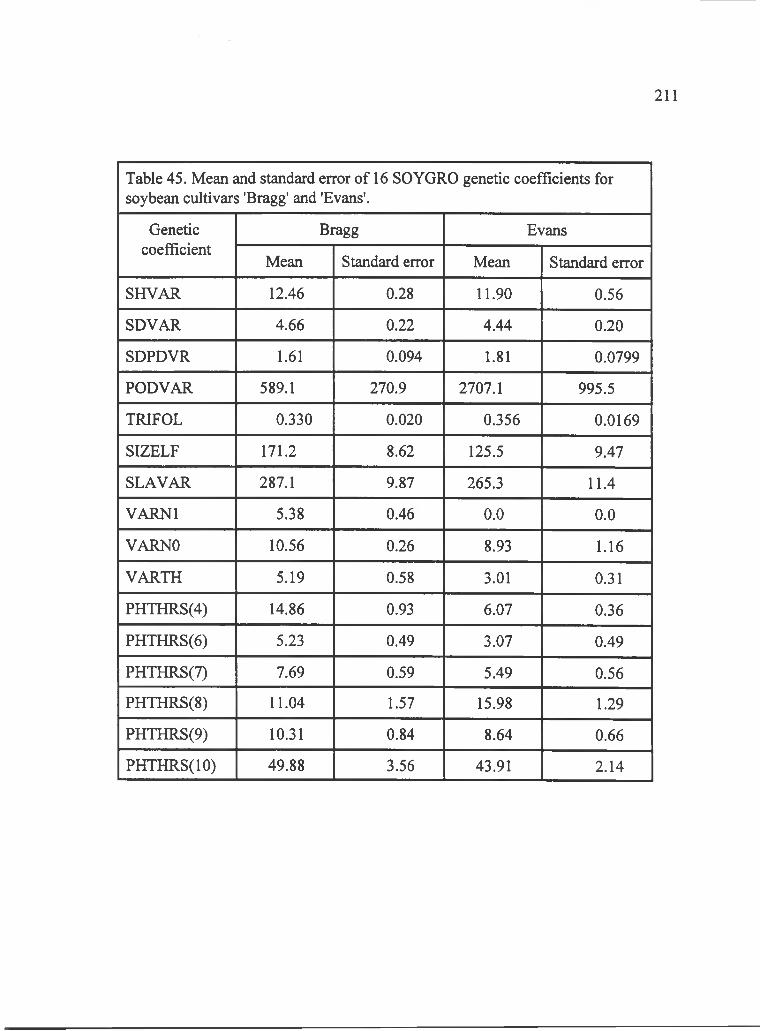
211
Table 45. Mean and standard error of 16 SOYGRO genetic coefficients for soybean cultivars 'Bragg' and 'Evans'.
Geneticcoefficient
Bragg Evans
Mean Standard error Mean Standard error
SHVAR 12.46 0.28 11.90 0.56
SDVAR 4.66 0 . 2 2 4.44 0 . 2 0
SDPDVR 1.61 0.094 1.81 0.0799
PODVAR 589.1 270.9 2707.1 995.5
TRIFOL 0.330 0 . 0 2 0 0.356 0.0169
SIZELF 171.2 8.62 125.5 9.47
SLAVAR 287.1 9.87 265.3 11.4
VARNl 5.38 0.46 0 . 0 0 . 0
VARNO 10.56 0.26 8.93 1.16
VARTH 5.19 0.58 3.01 0.31
PHTHRS(4) 14.86 0.93 6.07 0.36
PHTHRS(6 ) 5.23 0.49 3.07 0.49
PHTHRS(7) 7.69 0.59 5.49 0.56
PHTHRS(8 ) 11.04 1.57 15.98 1.29
PHTHRS(9) 10.31 0.84 8.64 0 . 6 6
PHTHRS(IO) 49.88 3.56 43.91 2.14

212
Table 46. Mean and standard error of 16 SOYGRO genetic coefficients for soybean cultivars 'Jupiter' and 'Williams'.
Geneticcoefficient
Jupiter Williams
mean standard error mean standard error
SHVAR 11.77 0.45 14.15 0.61
SDVAR 4.46 0.46 4.93 0.14
SDPDVR 1.44 0.083 1.98 0.13
PODVAR 481.1 94.0 2131.8 1749.6
TRIFOL 0.328 0.019 0.418 0.0240
SIZELF 266.5 15.4 195.0 16.2
SLAVAR 252.4 11.9 289.0 11.9
VARNl na na 2 . 2 0 1.28
VARNO 10.45 0.45 9.48 0.64
VARTH 1.38 0 . 0 5.29 0.92
PHTHRS(4) 39.78 5.12 7.08 0.46
PHTHRS(6 ) 10.83 1.49 5.21 0.80
PHTHRS(7) 14.59 1.75 7.48 0.84
PHTHRS(8 ) 7.43 1.40 15.91 1.67
PHTHRS(9) 14.16 1.52 10.31 0.91
PHTHRS(IO) 57.63 3.64 44.08 2.58
results, while the second factorial experiment was included to determine whether
photoperiod affected the importance of genetic coefficient contribution.
A sensitivity analysis for CERES-Maize genetic coefficients was performed
using a 2* unreplicated full factorial design. Eight coefficients in CERES-Maize were
varied ± one and two standard errors from the mean (Tables 47 and 48; see Table 13
for genetic coefficient definitions) in separate analyses. The mean minus standard
error and mean plus standard error of the eight coefficients was combined in a full
factorial to create 256 'genotypes' that were put into the genetic files for simulation.
The genetic file was modified to accommodate the extra coefficients P9, XLPGDD,
and PCHRON. The simulation conditions were identical to the conditions for
SOYGRO described above. However, the photoperiod calculations in CERES-Maize
included civil twilight. Therefore, photoperiods on 1 April and 21 June were 13.06
and 14.23 h at 20.85° latitude, and 13.52 and 16.23 h at 40.85° latitude.
Results from the simulation of the 256 'genotypes' for SOYGRO and CERES-
Maize were subjected to analysis o f variance to determine the genetic coefficients that
were associated with model bias. Yield and aboveground biomass were selected as
dependent variables from the simulation output for analysis of variance. These two
variables were considered important because they integrate many of the processes in
the models (Furbringer and Borchiellini, 1993). In the analysis o f variance for
SOYGRO, all main effects and two-factor interactions were specified in the statistical
model, the remaining sums of squares were pooled as experimental error. For
213
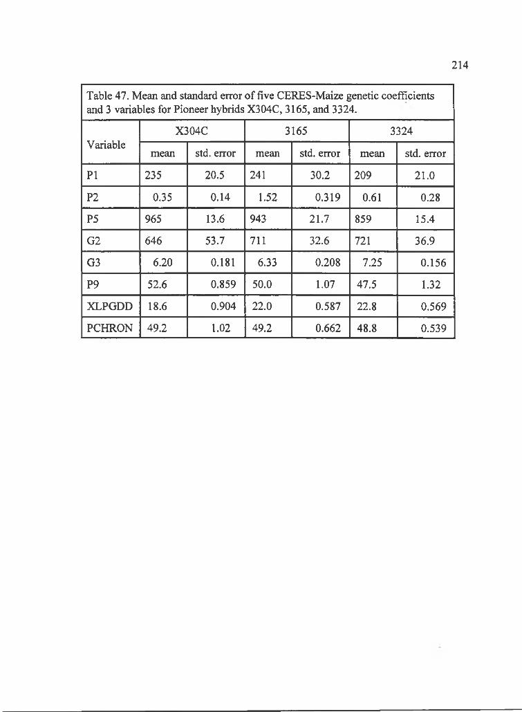
214
Table 47. Mean and standard error of five CERES-Maize genetic coefficients and 3 variables for Pioneer hybrids X304C, 3165, and 3324.
VariableX304C 3165 3324
mean std. error mean std. error mean std. error
PI 235 20.5 241 30.2 209 2 1 . 0
P2 0.35 0.14 1.52 0.319 0.61 0.28
P5 965 13.6 943 21.7 859 15.4
G2 646 53.7 711 32.6 721 36.9
G3 6 . 2 0 0.181 6.33 0.208 7.25 0.156
P9 52.6 0.859 50.0 1.07 47.5 1.32
XLPGDD 18.6 0.904 2 2 . 0 0.587 2 2 . 8 0.569
PCHRON 49.2 1 . 0 2 49.2 0.662 48.8 0.539
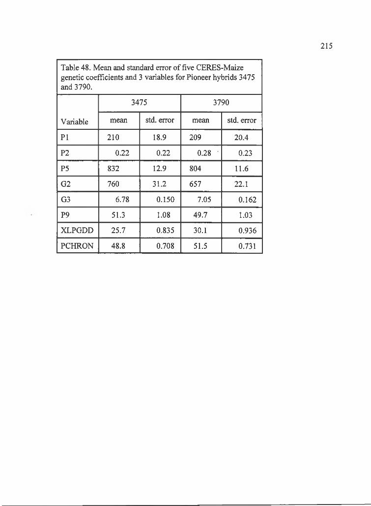
215
Table 48. Mean and standard error of five CERES-Maize genetic coefficients and 3 variables for Pioneer hybrids 3475 and 3790.
Variable
3475 3790
mean std. error mean std. error
PI 2 1 0 18.9 209 20.4
P2 0 . 2 2 0 . 2 2 0.28 ■ 0.23
P5 832 12.9 804 1 1 . 6
G2 760 31.2 657 2 2 . 1
G3 6.78 0.150 7.05 0.162
P9 51.3 1.08 49.7 1.03
XLPGDD 25.7 0.835 30.1 0.936
PCHRON 48.8 0.708 51.5 0.731
CERES-Maize, all four- to eight-factor interactions were assumed negligible and,
therefore, were pooled to estimate experimental error (Milliken and Johnson, 1989).
As an additional indicator of importance to model bias, the percentage of total
variation was calculated for each effect as.
216
% o f total variation = x 100SmS. total
where s.s. effect was an effect sum of squares and s.s. total was the total sum of
squares (Jain, 1991). The effects that were significant and accounted for a large
portion of the variation in yield or biomass was considered important to model bias.
Results
Results from the analysis of variance for the sensitivity analysis simulations
are in Tables 49 to 6 6 . The reported values are sum of squares for effects that
accounted for 2 % or greater of the total sums of squares.
The percentage of total variation was used to interpret the results. The
sensitivity analysis for yield and aboveground biomass performed on SOYGRO
genetic coefficients at ± two standard errors cannot be interpreted using classical
sensitivity analysis. All cuitivars showed that main effects decreased in percentage of
total sums of squares for yield and aboveground biomass while interaction effect
percentages increased as the level of each factor increased (Tables 49 to 56). The
increase in interactions indicated that the relation between the effect input values and
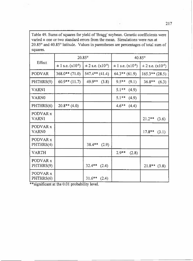
217
Table 49. Sums of squares for yield of'Bragg' soybean. Genetic coefficients were varied ± one or two standard errors from the mean. Simulations were run at 20.85° and 40.85° latitude. Values in parentheses are percentages of total sum of squares.
Effect20.85° 40.85°
± 1 s.e. (xlO-^) ± 2 s.e. (xlO- ') ± 1 s.e. (xlO"^) ± 2 s.e. (xlO-®)
PODVAR 368.0** (71.0) 547.4** (41.4) 64.3** (61.9) 165.3** (28.5)
PHTHRS(9) 60.9** (11.7) 49.9** (3.8) 9.5** (9.1) 36.8** (6.3)
VARNl 5.1** (4.9)
VARNO 5.1** (4.9)
PHTHRS(6 ) 20.8** (4.0) 4.6** (4.4)
PODVAR X VARNl 21.2** (3.6)
PODVARX VARNO 17.8** (3.1)
PODVARX PHTHRS(4) 38.4** (2.9)
VARTH 2.9** (2.8)
PODVARX PHTHRS(9) 32.4** (2.4) 21.8** (3.8)
PODVAR X PHTHRS(6 ) 31.6** (2.4)
♦♦significant at the 0 . 0 1 probability level.
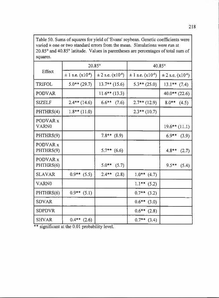
218
Table 50. Sums of squares for yield of'Evans' soybean. Genetic coefficients were varied ± one or two standard errors from the mean. Simulations were run at 20.85° and 40.85° latitude. Values in parentheses are percentages o f total sum of squares.
Effect20.85° 40.85°
± 1 s.e. (xlO"*) ± 2 s.e. (xlO'*) ± 1 s.e. (xlO-®) ± 2 s.e. (xlO"*)
TRIFOL 5.0** (29.7) 13.7** (15.6) 5.3** (25.0) 13.1** (7.4)
PODVAR 11.6** (13.3) 40.0** (22.6)
SIZELF 2.4** (14.6) 6 .6 ** (7.6) 2.7** (12.9) 8.0** (4.5)
PHTHRS(4) 1 .8 ** ( 1 1 .0 ) 2.3** (10.7)
PODVARX VARNO 19.6** (11.1)
PHTHRS(9) 7.8** (8.9) 6.9** (3.9)
PODVAR X PHTHRS(9) 5.7** (6 .6 ) 4.8** (2.7)
PODVARX PHTHRS(6 ) 5.0** (5.7) 9.5** (5.4)
SLAVAR 0.9** (5.5) 2.4** (2.8) 1.0** (4.7)
VARNO 1.1** (5.2)
PHTHRS(6 ) 0.9** (5.1) 0.7** (3.2)
SDVAR 0.6** (3.0)
SDPDVR 0 .6 ** (2 .8 )
SHVAR 0.4** (2.6) 0.7** (3.4)** significant at the 0 . 0 1 probability level.
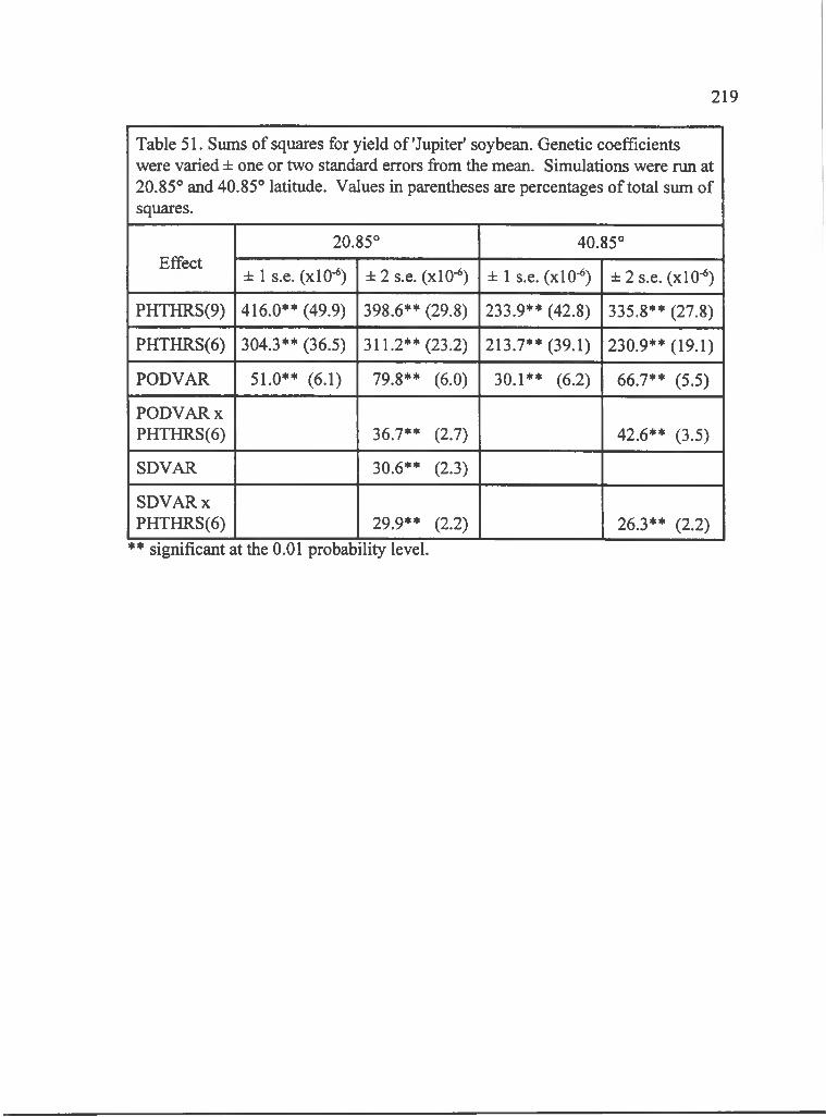
219
Table 51. Sums of squares for yield of'Jupiter' soybean. Genetic coefficients were varied ± one or two standard errors from the mean. Simulations were run at 20.85° and 40.85° latitude. Values in parentheses are percentages of total sum of squares.
Effect20.85° 40.85°
± 1 s.e. (xlO-*) ± 2 s.e. (x 1 0 - ) ± 1 s.e. (xlO-") ± 2 s.e. (xlO-*)
PHTHRS(9) 416.0** (49.9) 398.6** (29.8) 233.9** (42.8) 335.8** (27.8)
PHTHRS(6 ) 304.3** (36.5) 311.2** (23.2) 213.7** (39.1) 230.9** (19.1)
PODVAR 51.0** (6.1) 79.8** (6.0) 30.1** (6.2) 66.7** (5.5)
PODVARX PHTHRS(6 ) 36.7** (2.7) 42.6** (3.5)
SDVAR 30.6** (2.3)
SDVARX PHTHRS(6 ) 29.9** (2.2) 26.3** (2.2)
** significant at the 0 . 0 1 probability level.
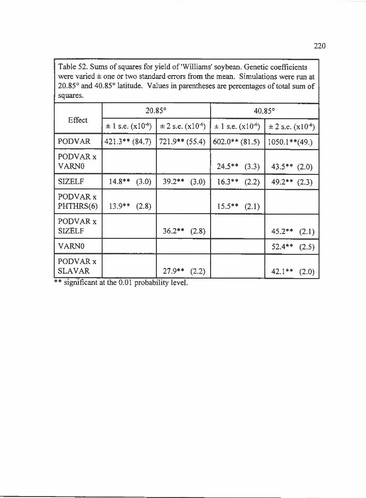
220
Table 52. Sums of squares for yield of'Williams' soybean. Genetic coefficients were varied ± one or two standard errors from the mean. Simulations were run at 20.85° and 40.85° latitude. Values in parentheses are percentages o f total sum of squares.
Effect20.85° 40.85°
± 1 s.e. (xlO-^) ± 2 s.e. (xlO-*') ± 1 s.e. (xlO-^) ± 2 s.e. (xlO- ')
PODVAR 421.3** (84.7) 721.9** (55.4) 602.0** (81.5) 1050.1**(49.)
PODVARX VARNO 24.5** (3.3) 43.5** (2.0)
SIZELF 14.8** (3.0) 39.2** (3.0) 16.3** (2.2) 49.2** (2.3)
PODVARX PHTHRS(6 ) 13.9** (2.8) 15.5** (2.1)
PODVARX SIZELF 36.2** (2.8) 45.2** (2.1)
VARNO 52.4** (2.5)
PODVARX SLAVAR 27.9** (2.2) 42.1** (2.0)
** significant at the 0 . 0 1 probability level.
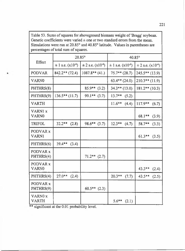
221
Table 53. Sums of squares for aboveground biomass weight of'Bragg' soybean. Genetic coefficients were varied ± one or two standard errors from the mean. Simulations were run at 20.85° and 40.85° latitude. Values in parentheses are percentages of total sum of squares.
Effect20.85° 40.85°
± 1 s.e. (xlO"*) ± 2 s.e. (xlO- ') ± 1 s.e. (xlO-«) ± 2 s.e. (xlO-'')
PODVAR 842.2** (72.4) 1087.8** (41.) 75.7** (28.7) 245.5** (13.9)
VARNO 63.4** (24.0) 210.3** (11.9)
PHTHRS(8 ) 85.9** (3.2) 34.3** (13.0) 181.2** (10.3)
PHTHRS(9) 136.5** (11.7) 99.1** (3.7) 13.7** (5.2)
VARTH 11.6** (4.4) 117.9** (6.7)
VARNl X VARNO 68.1** (3.9)
TRIFOL 32.2** (2.8) 98.6** (3.7) 12.3** (4.7) 58.7** (3.3)
PODVARX VARNl 61.3** (3.5)
PHTHRS(6 ) 39.4** (3.4)
PODVARX PHTHRS(4) 71.2** (2.7)
PODVARX VARNO 43.3** (2.4)
PHTHRS(4) 27.0** (2.4) 20.3** (7.7) 43.5** (2.5)
PODVAR X PHTHRS(9) 60.5** (2.3)
VARNOX VARTH 5.6** (2.1)
significant at the 0 . 0 1 probability level.
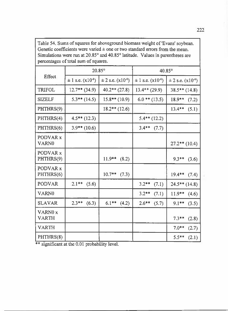
222
Table 54. Sums of squares for aboveground biomass weight of'Evans' soybean. Genetic coefficients were varied ± one or two standard errors from the mean. Simulations were run at 20.85° and 40.85° latitude. Values in parentheses are percentages of total sum of squares.
Effect20.85° 40.85°
± 1 s.e. (xlO"®) ± 2 s.e. (x l 0 ‘®) ± 1 s.e. (xlO'®) ± 2 s.e. (xlO"*)
TRIFOL 12.7** (34.9) 40.2** (27.8) 13.4** (29.9) 38.5** (14.8)
SIZELF 5.3** (14.5) 15.8** (10.9) 6.0 ** (13.5) 18.9** (7.2)
PHTHRS(9) 18.2** ( 1 2 .6 ) 13.4** (5.1)
PHTHRS(4) 4.5** (12.3) 5.4** (12.2)
PHTHRS(6 ) 3.9** (10.6) 3.4** (7.7)
PODVARX VARNO 27.2** (10.4)
PODVARX PHTHRS(9) 11.9** (8.2) 9.3** (3.6)
PODVAR X PHTHRS(6 ) 10.7** (7.3) 19.4** (7.4)
PODVAR 2.1** (5.6) 3.2** (7.1) 24.5** (14.8)
VARNO 3.2** (7.1) 11.9** (4.6)
SLAVAR 2.3** (6.3) 6.1** (4.2) 2.6** (5.7) 9.1** (3.5)
VARNO X VARTH 7.3** (2.8)
VARTH 7.0** (2.7)
PHTHRS(8 ) 5.5** (2.1)**significant at the 0 . 0 1 probability level.
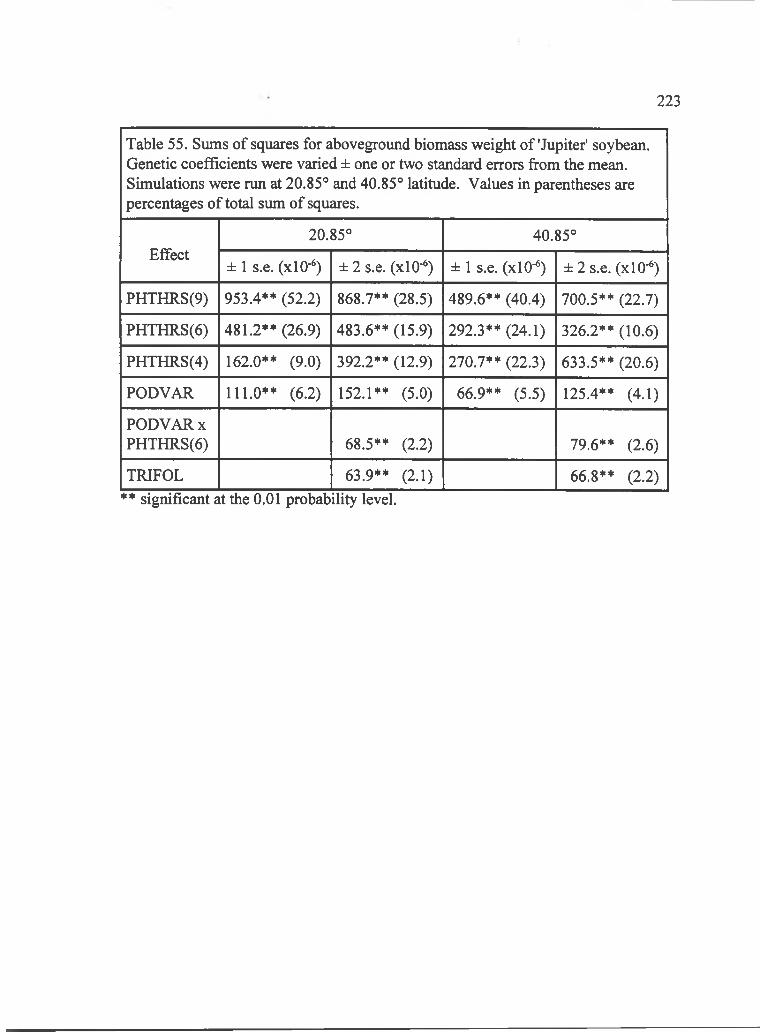
223
Table 55. Sums of squares for aboveground biomass weight of'Jupiter' soybean. Genetic coefficients were varied ± one or two standard errors from the mean. Simulations were run at 20.85° and 40.85° latitude. Values in parentheses are percentages of total sum of squares.
Effect20.85° 40.85°
± 1 s.e. (xlO"*) ± 2 s .e .(x l 0 -") ± 1 s.e. (xlO-®) ± 2 s.e. (xlO-^)
PHTHRS(9) 953.4** (52.2) 868.7** (28.5) 489.6** (40.4) 700.5** (22.7)
PHTHRS(6 ) 481.2** (26.9) 483.6** (15.9) 292.3** (24.1) 326.2** (10.6)
PHTHRS(4) 162.0** (9.0) 392.2** (12.9) 270.7** (22.3) 633.5** (20.6)
PODVAR 1 1 1 .0 ** (6 .2 ) 152.1** (5.0) 66.9** (5.5) 125.4** (4.1)
PODVARX PHTHRS(6 ) 68.5** (2.2) 79.6** (2.6)
TRIFOL 63.9** (2.1) 6 6 .8 ** (2 .2 )** significant at the 0 . 0 1 probability level.
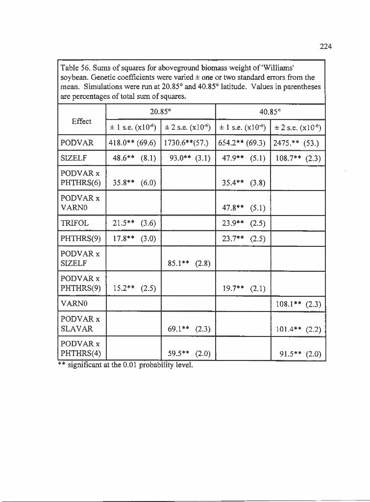
224
Table 56. Sums of squares for aboveground biomass weight of'Williams' soybean. Genetic coefficients were varied ± one or two standard errors from the mean. Simulations were run at 20.85° and 40.85° latitude. Values in parentheses are percentages of total sum of squares.
Effect20.85° 40.85°
± 1 s.e. (xlO- ') ± 2 s.e. (xlO-") ± 1 s.e. (xlO"*) ± 2 s.e. (X1 0 - )
PODVAR 418.0** (69.6) 1730.6**(57.) 654.2** (69.3) 2475.** (53.)
SIZELF 48.6** (8.1) 93.0** (3.1) 47.9** (5.1) 108.7** (2.3)
PODVARX PHTHRS(6 ) 35.8** (6.0) 35.4** (3.8)
PODVAR X VARNO 47.8** (5.1)
TRIFOL 21.5** (3.6) 23.9** (2.5)
PHTFIRS(9) 17.8** (3.0) 23.7** (2.5)
PODVAR X SIZELF 85.1** (2.8)
PODVARX PHTHRS(9) 15.2** (2.5) 19.7** (2.1)
VARNO 108.1** (2.3)
PODVARX SLAVAR 69.1** (2.3) 101.4** (2.2)
PODVAR X PHTHRS(4) 59.5** (2.0) 91.5** (2.0)
** significant at the 0 . 0 1 probability level.
the simulation output, yield and biomass, was non-linear. Hence, classical sensitivity
analysis would not be applicable for SOYGRO genetic coefficients (Havens and
Fontaine, 1991). Furthermore, analysis of variance showed that all reported effects
were highly significant for SOYGRO and CERES-Maize, probably because of the
very small experimental error. Since classical sensitivity analysis cannot be applied
and analysis of variance was too sensitive, percentage of total sums of squares was
the basis for effect differentiation.
Generally, latitude did not affect the proportion of variation that SOYGRO
genetic coefficients had on yield or aboveground biomass. The percentage of total
sums of squares for each effect showed little difference when simulated latitude was
changed fi-om 20.85° to 40.85° (Tables 49 to 56). In some cases, the photoperiod
sensitivity genetic coefficients VARNO, VARTH and VARNl became prominent at
40.85°, but the proportion of variation was small, typically less than 5% points. The
one exception was aboveground biomass for 'Bragg' where the proportion of variation
drastically changed with latitude (Table 53). Otherwise, latitude was not a factor that
would change the results of the sensitivity analysis.
The SOYGRO genetic coefficients that account for most of the variation in
yield were PODVAR and PHTHRS(9). For cuitivars 'Bragg' (Table 49) and
'Williams' (Table 52), PODVAR accounted for most of the variation in yield, up to
85%. PODVAR was a major contributor to variation in yield at high latitude and ±
two standard errors for 'Evans' (Table 50), but was a minor contributor to variation in
225

yield for 'Jupiter' (Table 51). PHTHRS(9) contributed up to 50% of yield variation
for 'Jupiter', but was a minor contributor for the other cultivars. 'Evans' had TRIFOL
as a major source of variation for yield, 7 to 30%, and 'Jupiter' had PHTHRS(6 ), 19 to
39%, as a major contributor. However, no other cultivar had these effects as major
contributors in yield variation. Generally, PODVAR and PHTHRS(9) were the
greatest contributor to variation in yield over most cultivars.
A pattern similar to yield was foimd for effect contribution to aboveground
biomass variation. PODVAR was an important contributor to aboveground biomass
variation for 'Bragg' and 'Williams', 29 to 72% and 69%, respectively (Tables 53 and
56). For 'Evans', the major contributor to variation was TRIFOL, 15 to 35% (Table
53). PHTHRS(9) was the major source of aboveground biomass variation for
'Jupiter', 23 to 52%. Generally, PODVAR was the major source of aboveground
biomass variation, but TRIFOL and PHTHRS(9) were also contributors for some
cultivars.
Latitude did not affect the proportions of yield or aboveground biomass
variation in CERES-Maize. Comparing various effects that accounted for the
proportion of yield and aboveground biomass variation, the difference among
latitudes was typically less than 5% points (Tables 57 to 6 6 ). Therefore, latitude was
considered a negligible factor in the sensitivity analysis.
The CERES-Maize genetic coefficient G2 was consistently the greatest
contributor to yield variation. Over all Pioneer hybrids, G2 accounted for 33 to 65%
226
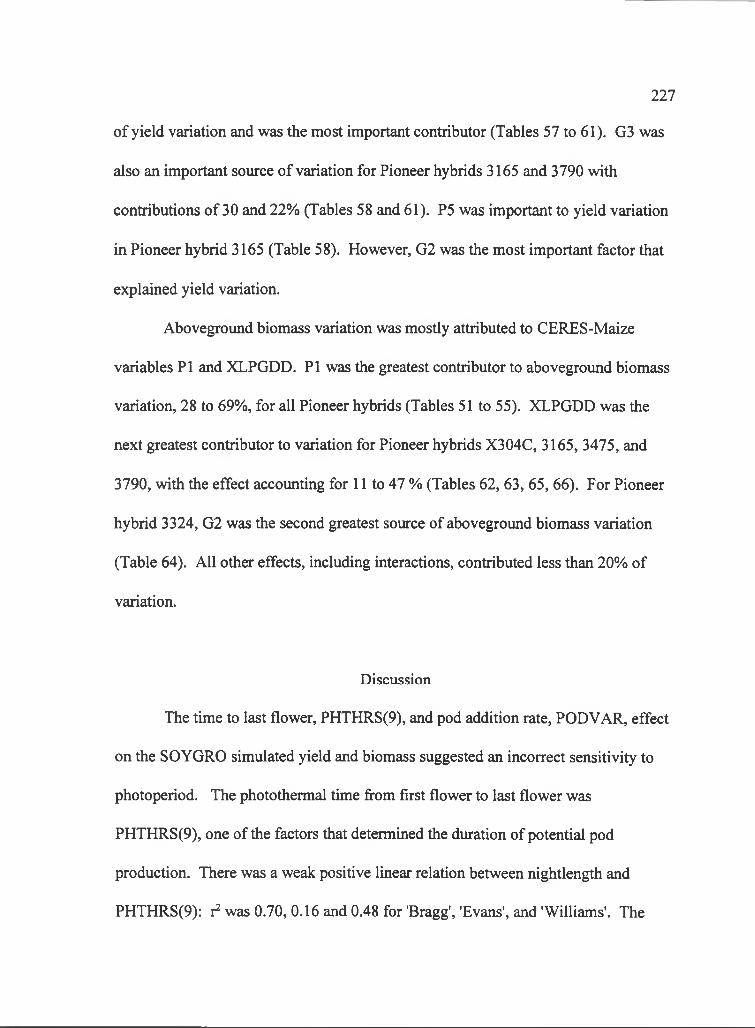
of yield variation and was the most important contributor (Tables 57 to 61). G3 was
also an important source of variation for Pioneer hybrids 3165 and 3790 with
contributions o f 30 and 22% (Tables 58 and 61). P5 was important to yield variation
in Pioneer hybrid 3165 (Table 58). However, G2 was the most important factor that
explained yield variation.
Aboveground biomass variation was mostly attributed to CERES-Maize
variables PI and XLPGDD. PI was the greatest contributor to aboveground biomass
variation, 28 to 69%, for all Pioneer hybrids (Tables 51 to 55). XLPGDD was the
next greatest contributor to variation for Pioneer hybrids X304C, 3165, 3475, and
3790, with the effect accoimting for 11 to 47 % (Tables 62, 63, 65, 6 6 ). For Pioneer
hybrid 3324, G2 was the second greatest source of aboveground biomass variation
(Table 64). All other effects, including interactions, contributed less than 20% of
variation.
Discussion
The time to last flower, PHTHRS(9), and pod addition rate, PODVAR, effect
on the SOYGRO simulated yield and biomass suggested an incorrect sensitivity to
photoperiod. The photothermal time from first flower to last flower was
PHTHRS(9), one of the factors that determined the duration of potential pod
production. There was a weak positive linear relation between nightlength and
PHTHRS(9): r 'w as 0.70, 0.16 and 0.48 for'Bragg','Evans', and'Williams'. The
Ill
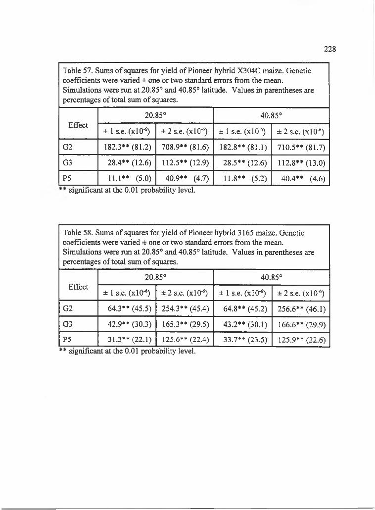
228
Table 57. Sums of squares for yield of Pioneer hybrid X304C maize. Genetic coefficients were varied ± one or two standard errors from the mean. Simulations were run at 20.85° and 40.85° latitude. Values in parentheses are percentages of total sum of squares.
Effect20.85° 40.85°
± 1 s.e. (xlO"^) ± 2 s.e. (xlO"^) ± 1 s.e. (xlO-*) ± 2 s.e. (xlO-")
G2 182.3** (81.2) 708.9** (81.6) 182.8** (81.1) 710.5** (81.7)
G3 28.4** (12.6) 112.5** (12.9) 28.5** (12.6) 112.8** (13.0)
P5 11.1** (5.0) 40.9** (4.7) 11.8** (5.2) 40.4** (4.6)significant at the 0 . 0 1 probability level.
Table 58. Sums of squares for yield of Pioneer hybrid 3165 maize. Genetic coefficients were varied ± one or two standard errors from the mean. Simulations were run at 20.85° and 40.85° latitude. Values in parentheses are percentages of total sum of squares.
Effect20.85° 40.85°
± 1 s.e. (xlO-^) ± 2 s.e. (xlO- *) ± 1 s.e. (xlO- ') ± 2 s.e. (xlO-")
G2 64.3** (45.5) 254.3** (45.4) 64.8** (45.2) 256.6** (46.1)
G3 42.9** (30.3) 165.3** (29.5) 43.2** (30.1) 166.6** (29.9)
P5 31.3** (22.1) 125.6** (22.4) 33.7** (23.5) 125.9** (22.6)** significant at the 0 . 0 1 probability level.
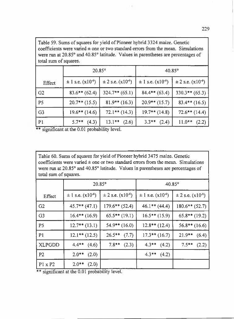
229
Table 59. Sums of squares for yield of Pioneer hybrid 3324 maize. Genetic coefficients were varied ± one or two standard errors from the mean. Simulations were run at 20.85° and 40.85° latitude. Values in parentheses are percentages of total sum of squares.
Effect
20.85° 40.85°
± 1 s.e. (xlO-^) ± 2 s.e. (xlO-*) ± 1 s.e. (xlO-^) ± 2 s.e. (xlO-^)
G2 83.6** (62.4) 324.7** (65.1) 84.4** (63.4) 330.3** (65.3)
P5 20.7** (15.5) 81.9** (16.3) 20.9** (15.7) 83.4** (16.5)
G3 19.6** (14.6) 72.1** (14.3) 19.7** (14.8) 72.6** (14.4)
PI 5.7** (4.3) 13.1** (2.6) 3.3** (2.4) 1 1 .0 ** (2 .2 )significant at the 0 . 0 1 probability level.
Table 60. Sums of squares for yield of Pioneer hybrid 3475 maize. Genetic coefficients were varied ± one or two standard errors from the mean. Simulations were run at 20.85° and 40.85° latitude. Values in parentheses are percentages of total sum of squares.
Effect
20.85° 40.85°
± 1 s.e. (xlO''^) ± 2 s.e. (xlO-®) ± 1 s.e. (xlO- ') ± 2 s.e. (xlO-^)
G2 45.7** (47.1) 179.6** (52.4) 46.1** (44.4) 180.6** (52.7)
G3 16.4** (16.9) 65.5** (19.1) 16.5** (15.9) 65.8** (19.2)
P5 12.7** (13.1) 54.9** (16.0) 12.8** (12.4) 56.8** (16.6)
PI 12.1** (12.5) 26.5** (7.7) 17.3** (16.7) 21.9** (6.4)
XLPGDD 4.4** (4.6) 7.8** (2.3) 4.3** (4.2) 7.5** (2.2)
P2 2 .0 ** (2 .0 ) 4.3** (4.2)
PI xP2 2 .0 ** (2 .0 )** significant at the 0 . 0 1 proba uility level.
230
Table 61. Sums of squares for yield of Pioneer hybrid 3790 maize. Genetic coefficients were varied ± one or two standard errors from the mean. Simulations were run at 20.85° and 40.85° latitude. Values in parentheses are percentages of total sum of squares.
Effect
20.85° 40.85°
± 1 s.e. (xlO- *) ± 2 s.e. (xlO-^) ± 1 s.e. (xlO- ') ± 2 s.e. (xlO-'')
G2 20.0** (36.3) 79.2** (33.5) 20.4** (38.6) 82.1** (36.3)
G3 1 2 . 1 ** (2 2 .0 ) 47.1** (19.9) 12.4** (23.4) 48.6** (21.5)
P5 7.6** (13.7) 33.6** (14.2) 7.4** (14.1) 34.1** (15.1)
PI 6 .6 ** ( 1 2 .0 ) 56.2** (24.2) 5.9** (11.2) 35.8** (15.8)
XLPGDD 6.9** (12.5) 13.5** (5.7) 1.7** (3.3) 12.5** (5.5)
P2 1.7** (3.3) 7.0** (3.1)
P 2xXLPGDD 1.7** (3.3)
significant at the 0 . 0 1 probability level.
Table 62. Sums of squares for aboveground biomass weight of Pioneer hybrid X304C maize. Genetic coefficients were varied ± one or two standard errors from the mean. Simulations were run at 20.85° and 40.85° latitude. Values in parentheses are percentages o f total sum o f squares.
Effect
20.85° 40.85°
± 1 s.e. (xlO-^) ± 2 s.e. (xlO-®) ± 1 s.e. (xlO-^) ± 2 s.e. (xlO"*)
PI 775.2** (52.5) 1276.7**(33.5) 484.5** (39.0) 1410.7**(35.5)
XLPGDD 537.0** (36.4) 1802.1 **(47.2) 544.1** (43.8) 1720.4**(43.3)
G2 130.2** (8 .8 ) 506.2** (13.3) 130.5** (10.5) 507.3** (12.8)
PI xP2 34.0** (2.7)
G3 80.3** (2.1) 80.5** (2.0)** significant at the 0 . 0 1 probalrility level.
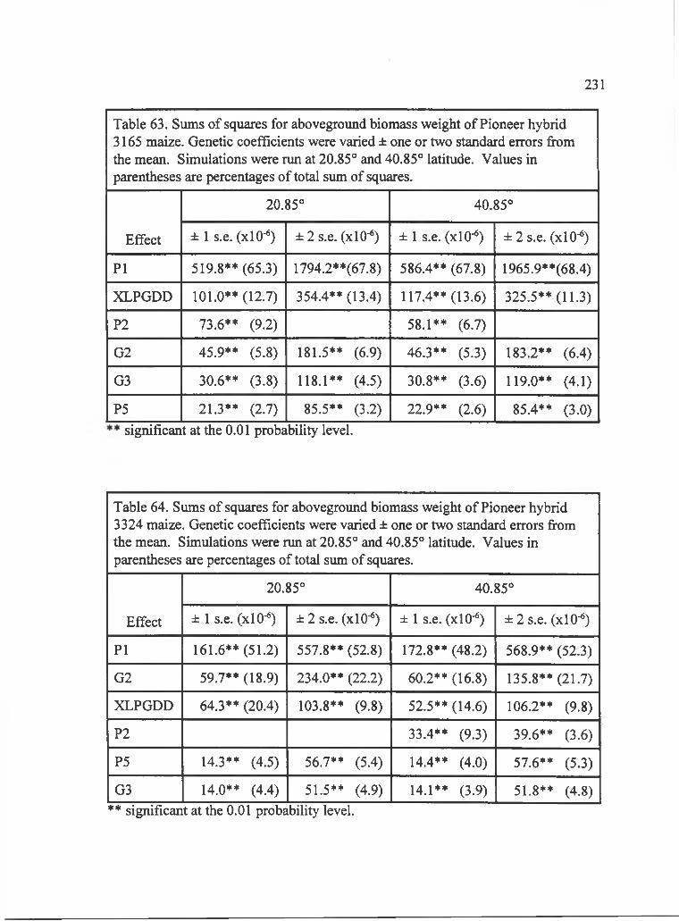
231
Table 63. Sums of squares for aboveground biomass weight of Pioneer hybrid 3165 maize. Genetic coefficients were varied ± one or two standard errors from the mean. Simulations were run at 20.85° and 40.85° latitude. Values in parentheses are percentages of total sum of squares.
Effect
20.85° 40.85°
± 1 s.e. (xlO- *) ± 2 s.e. (xlO- ') ± 1 s.e. (xlO-^) ± 2 s.e. (xlO-^)
PI 519.8** (65.3) 1794.2**(67.8) 586.4** (67.8) 1965.9**(68.4)
XLPGDD 101.0** (12.7) 354.4** (13.4) 117.4** (13.6) 325.5** (11.3)
P2 73.6** (9.2) 58.1** (6.7)
G2 45.9** (5.8) 181.5** (6.9) 46.3** (5.3) 183.2** (6.4)
G3 30.6** (3.8) 118.1** (4.5) 30.8** (3.6) 119.0** (4.1)
P5 21.3** (2.7) 85.5** (3.2) 22.9** (2.6) 85.4** (3.0)significant at the 0 . 0 1 probability level.
Table 64. Sums of squares for abovegroimd biomass weight of Pioneer hybrid 3324 maize. Genetic coefficients were varied ± one or two standard errors from the mean. Simulations were run at 20.85° and 40.85° latitude. Values in parentheses are percentages of total sum of squares.
Effect
20.85° 40.85°
± 1 s.e. (xlO-*) ± 2 s.e. (x 1 0 - ) ± 1 s.e. (xlO-'') ± 2 s.e. (xlO- ')
PI 161.6** (51.2) 557.8** (52.8) 172.8** (48.2) 568.9** (52.3)
G2 59.7** (18.9) 234.0** (22.2) 60.2** (16.8) 135.8** (21.7)
XLPGDD 64.3** (20.4) 103.8** (9.8) 52.5** (14.6) 106.2** (9.8)
P2 33.4** (9.3) 39.6** (3.6)
P5 14.3** (4.5) 56.7** (5.4) 14.4** (4.0) 57.6** (5.3)
G3 14.0** (4.4) 51.5** (4.9) 14.1** (3.9) 51.8** (4.8)** significant at the 0 . 0 1 probability level.
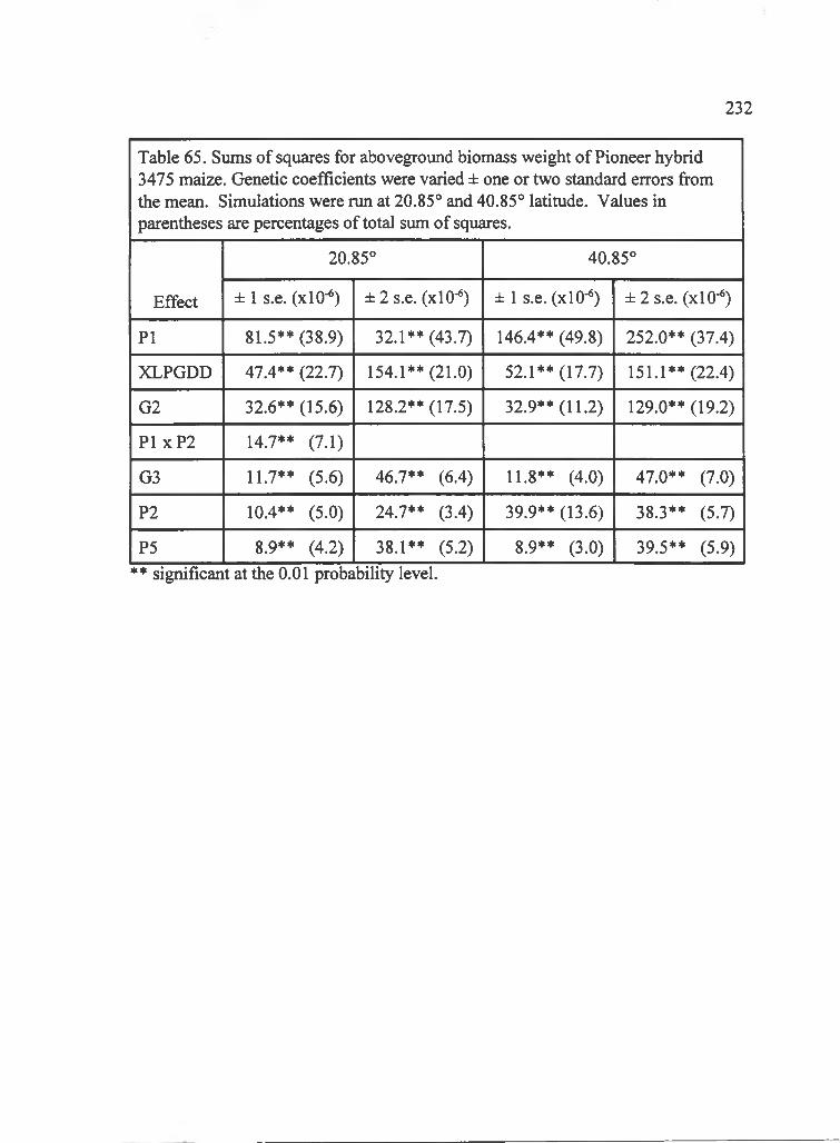
232
Table 65. Sums of squares for aboveground biomass weight of Pioneer hybrid 3475 maize. Genetic coefficients were varied ± one or two standard errors from the mean. Simulations were run at 20.85° and 40.85° latitude. Values in parentheses are percentages of total sum of squares.
Effect
20.85° 40.85°
± 1 s.e. (xlO-") ± 2 s.e. (xlO-*) ± 1 s.e. (xlO-'') ± 2 s.e. (xlO-*')
PI 81.5** (38.9) 32.1** (43.7) 146.4** (49.8) 252.0** (37.4)
XLPGDD 47.4** (22.7) 154.1** (21.0) 52.1** (17.7) 151.1** (22.4)
G2 32.6** (15.6) 128.2** (17.5) 32.9** (11.2) 129.0** (19.2)
PI xP2 14.7** (7.1)
G3 11.7** (5.6) 46.7** (6.4) 11.8** (4.0) 47.0** (7.0)
P2 10.4** (5.0) 24.7** (3.4) 39.9** (13.6) 38.3** (5.7)
P5 8.9** (4.2) 38.1** (5.2) 8.9** (3.0) 39.5** (5.9)** significant at the 0 . 0 1 probability level.
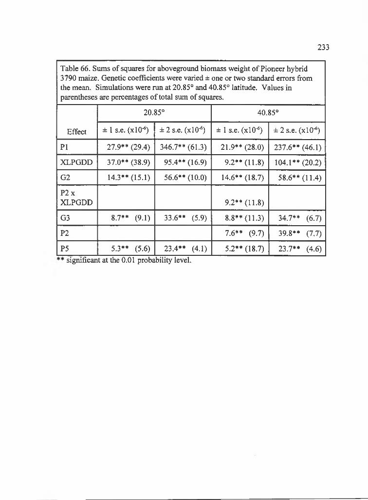
233
Table 6 6 . Sums of squares for abovegroimd biomass weight of Pioneer hybrid 3790 maize. Genetic coefficients were varied ± one or two standard errors from the mean. Simulations were run at 20.85° and 40.85° latitude. Values in parentheses are percentages of total sum of squares.
Effect
20.85° 40.85°
± 1 s.e. (xlO-< ) ± 2 s.e. (xlO-^) ± 1 s.e. (xlO-**) ± 2 s.e. (xlO-*)
PI 27.9** (29.4) 346.7** (61.3) 21.9** (28.0) 237.6** (46.1)
XLPGDD 37.0** (38.9) 95.4** (16.9) 9.2** (11.8) 104.1** (20.2)
G2 14.3** (15.1) 56.6** (10.0) 14.6** (18.7) 58.6** (11.4)
P 2xXLPGDD 9.2** (11.8)
G3 8.7** (9.1) 33.6** (5.9) 8 .8 ** (11.3) 34.7** (6.7)
P2 7.6** (9.7) 39.8** (7.7)
P5 5.3** (5.6) 23.4** (4.1) 5.2** (18.7) 23.7** (4.6)significant at the 0 . 0 1 probability level.

positive linear relation suggested that although PHTHRS(9) was in photothermal
units, the photoperiod sensitivity calculation underestimated the true effect. This
would result in a high PHTHRS(9) at long nightlength and low PHTHRS(9) at short
nightlength when fitting the PHTHRS(9) values to field observations. Grimm et al.
(1994) noted that soybean became more sensitive to photoperiod as plants developed
toward maturity and suggested that a new photothermal relation to soybean
development would be needed. This suggests that a different sensitivity to
photoperiod would be needed for flowering and post-flowering phases instead of the
same photoperiod sensitivity in all phases currently used in SOYGRO. The incorrect
specification for photothermal time likely caused the variation in PHTHRS(9), hence
the variation in time for potential pod production, that ultimately was manifested in
variation in yield and aboveground biomass.
The other important factor that affected yield and aboveground biomass, the
maximum rate of pod addition or PODVAR, may have be the pod abortion
relationship to photoperiod in SOYGRO. Once the number of flowers was set
according to the time of flowering and the flower production rate, pod number was
determined by multiplying the potential number of pod production, PODVAR, by
factors such as available amount of photosynthate, temperature, and photoperiod.
The photoperiod factor, called PODNIT, was defined as.
234
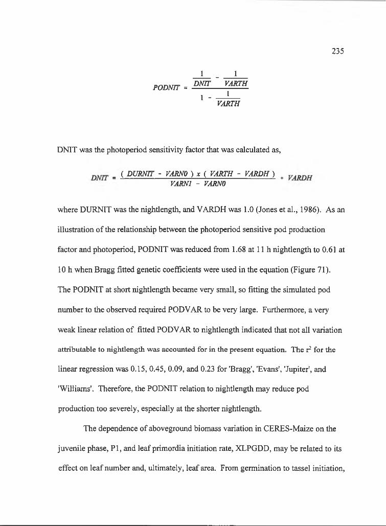
235
PODNTT =
1 _ 1 DNTT VARTH
1 - 1VARTH
DNIT was the photoperiod sensitivity factor that was calculated as,
_ ( DURNTT - VARNO ) x ( VARTH - VARDH ) VARNl - VARNO
where DURNIT was the nightlength, and VARDH was 1.0 (Jones et al., 1986). As an
illustration of the relationship between the photoperiod sensitive pod production
factor and photoperiod, PODNIT was reduced from 1.68 at 11 h nightlength to 0.61 at
10 h when Bragg fitted genetic coefficients were used in the equation (Figure 71).
The PODNIT at short nightlength became very small, so fitting the simulated pod
number to the observed required PODVAR to be very large. Furthermore, a very
weak linear relation of fitted PODVAR to nightlength indicated that not all variation
attributable to nightlength was accounted for in the present equation. The r’ for the
linear regression was 0.15, 0.45, 0.09, and 0.23 for 'Bragg', 'Evans', 'Jupiter', and
'Williams'. Therefore, the PODNIT relation to nightlength may reduce pod
production too severely, especially at the shorter nightlength.
The dependence of abovegroimd biomass variation in CERES-Maize on the
juvenile phase, PI, and leaf primordia initiation rate, XLPGDD, may be related to its
effect on leaf number and, ultimately, leaf area. From germination to tassel initiation.
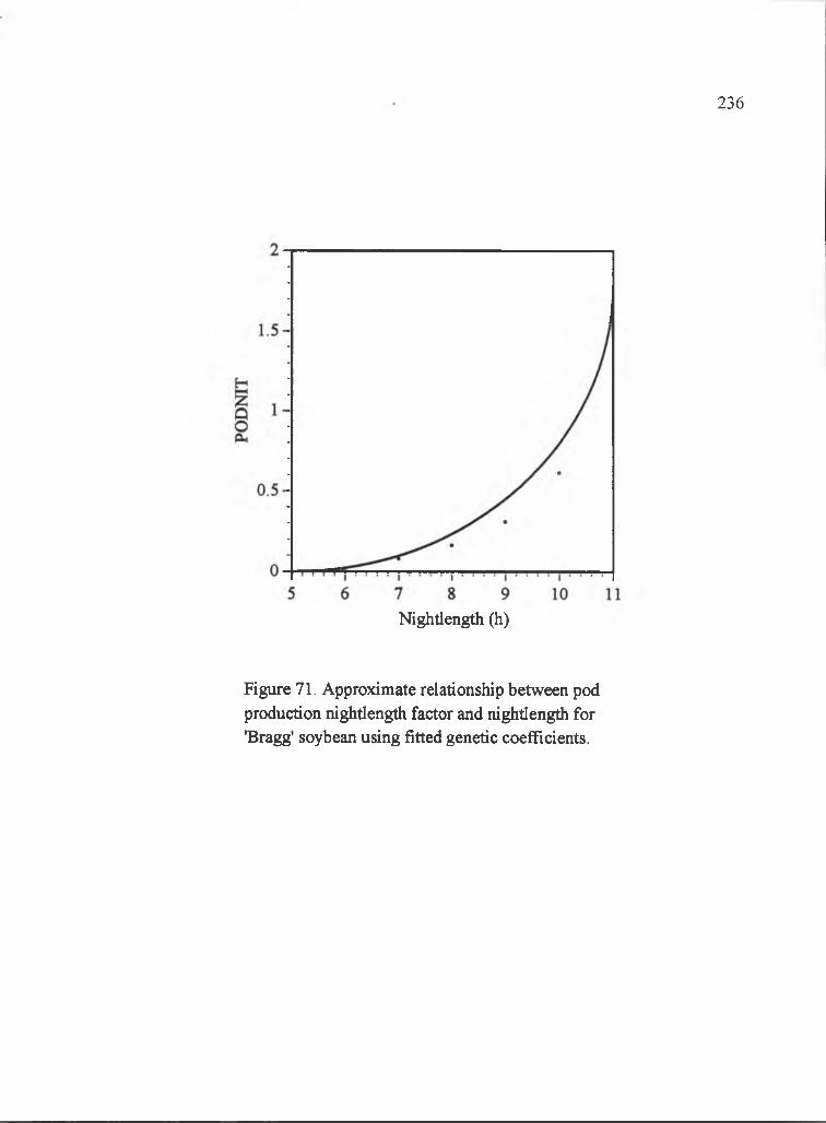
236
Nightlength (h)
Figure 71. Approximate relationship between pod production nightlength factor and nightlength for 'Bragg' soybean using fitted genetic coefficients.

CERES-Maize calculated that one leaf primordia was initiated every 21 growing
degree days (base temperature 8 °C) in addition to six leaf primordia already present
in the seed (Jones et al., 1986). The juvenile phase, PI, was a portion of the
germination to tassel initiation phase. Therefore, changing PI changes the leaf
number and leaf area. Likewise, changing the leaf primordia initiation rate would
change leaf number and area. Because potential carbohydrate production is
dependent on light interception, which in turn is dependent on leaf area, leaf area
influenced aboveground biomass accumulation.
The variation in PI may be partly attributable to the CERES-Maize
assumption that the photoperiod inductive phase began four days prior to tassel
initiation. In CERES-Maize, the photoperiod sensitive phase is assumed to start four
days prior to tassel initiation when photoperiod is less than the threshold, 1 2 . 5 h
(Jones et al., 1986). However, Kiniry et al. (1983) found that the photoperiod
sensitive phase started 4 to 8 days prior to tassel initiation. If the actual beginning of
the photoperiod sensitive phase was greater than the assumed four days, the
determined PI would vary with the ambient temperature: PI would be less in low
temperature than in high. The mean fitted PI determined at the cool site, Haleakala,
was 215.5 while at the warmer site PI was 226.0. The difference in PI between the
two sites indicated that the end of juvenile phase to tassel initiation may not be four
days. However, this difference was relatively small and can only partly account for
PI variation.
237
The leaf primordia initiation rate in CERES-Maize may also account for
aboveground biomass variation. CERES-Maize assumes leaf primordia initiation rate
is only dependent on temperature. Hence, the leaf primordia is calculated to initiate
at a set interval of growing degree days. However, photoperiod is known to affect
leaf primordia initiation rate (Grant, 1989). Warrington and Kanemasu (1983b)
found that leaf initiation rate increased as photoperiod increased, as much as 25%
faster, and that the effect was more pronounced under cool temperature. The fitted,
leaf primordia initiation rate, XLPGDD, showed a weak linear relation to
photoperiod. Linear regression o f XLPGDD on photoperiod had r of 0.66,0.33,
0.13, 0.46, and 0.35 for Pioneer hybrids X304C, 3165, 3324, 3475, and 3790. So,
specifying a photoperiod effect on leaf primordia initiation rate may increase the leaf
area and aboveground biomass response to daylength.
G2 was the factor that most affected yield in CERES-Maize and may be partly
related to leaf area problems discussed above. In CERES-Maize, the yield
component kernel number is a function o f the potential kernel nvimber, G2, and
photosynthate production from silking to beginning kernel growth (Jones et al.,
1986). Since photosynthate production is a function of leaf area, any bias in leaf area
calculation would be compensated for in the fitted G2, giving G2 greater variation.
So, G2 seemed to be a large factor in yield variation. Another factor in G2 variation
was its photoperiod dependence observed in Pioneer hybrid X304C. Photoperiod
238

effect on tassel-silking interval and kernel number is not a function in CERES-Maize,
so any effect would be absorbed in the fitted G2 causing variation.
Little work on the SOYGRO and CERES-Maize may produce much effect on
the applicability of these models to environments that differ especially in
photoperiod. The potential problems in SOYGRO and CERES-Maize that seemed
photoperiod related were identified. In SOYGRO, the relation between photoperiod
and photothermal time and the relations between nightlength and pod production
were important contributors to model bias in yield and biomass. CERES-Maize yield
and abovegroimd biomass bias seemed to be related to when the photoperiod
sensitive phase starts and the relation of leaf primordia initiation to photoperiod.
With the specification of these effects, the model bias should be reduced and the
applicability of the model increased to sites that widely differ in photoperiod.
239

CHAPTER 5
SUMMARY AND CONCLUSIONS
As model refinements are made, a standard set of data over many
environments will be needed to test the modifications. One of the major drawbacks
in modeling crop plants is the shortage of data sets to test a modified model. Usually,
modelers must develop data through field experimentation or borrow data sets.
However, the number and range of environments that these data sets represent are
usually limited, especially early in the development cycle. Hence, the models are not
well tested. A standard set of data to validate models should be developed from
environments that include extremes in temperature, photoperiod, solar radiation,
rainfall, soil water holding capacity, and soil pH. The standard data set to test models
against will not only allow quicker testing, but make comparisons among alternate
models uniform. Presently, judging the utility of alternate models is difficult because
the models are tested against different observed data sets. Therefore, data sets that
reflect the extremes in agricultural systems will be needed as models are refined to
simulate crop response to marginal conditions.
To increase the utility of the simulation model, genetic coefficients should be
easily determinable. Two methods to determine genetic coefficients for SOYGRO
and CERES-maize were evaluated. An explicit method to determine CERES-Maize
genetic coefficients worked fairly well for development, but not for growth. The
240

procedure to determine the growth coefficients from the real-system may have been
inadequately defined. The fitting method to determine genetic coefficients was able
to generate adequate development coefficients, but not growth coefficients for
SOYGRO and CERES-Maize. The problem may have been that the relations within
the model were not well validated in extreme conditions, so the model did not truly
reflect the real system. Then, fitting coefficients to match the real system resulted in
genetic coefficients that compensated for model biases. Seemingly, in a simple
method to derive genetic coefficients, the coefficients cannot be considered apart
from the model. Therefore, refinements in SOYGRO and CERES-Maize are needed
to improve this method to determine genetic coefficients.
Currently, the genetic coefficients for SOYGRO and CERES-Maize are
environment dependent. The growth genetic coefficients for SOYGRO and CERES-
Maize were dependent on environment as seen in the trends over photoperiods and
sites. This implies that the genetic coefficients determined in one environment cannot
be used to simulate crop growth in another environment, especially when the
environments greatly differ in photoperiod. To improve the models, more knowledge
of the interaction between environment and plant growth and development is
necessary. Under natural conditions, temperature and photoperiod are correlated.
Then, an empirical model based on field data would contain photoperiod or
temperature sensitivity with concomitant effects of the other built into the
environmental effects on crop development and growth. This model would not well
241

simulate crop development and growth where temperature and photoperiod are not
closely correlated such as along a mountain slope or tropical regions. Other
implications of the genetic coefficient dependency on environment are not well
understood at this time.
242

243
APPENDIX A Soybean data, summer 1988
Table A. 1 Soybean data from Haleakala Experiment Station, control photoperiod treatment.
INFORMATION REQUIRED FOR DETAILED DATA ANALYSIS
SOYBEAN GENETIC COEFFICIENT NURSERIES
INSTITUTENAME( INNAME) : IBSNATID (IN S T ID ): IB
RESEARCHER(S)NAME(RENAME) : R . OGOSHIID (R E SID ): RO
EXPERIMENTNAME (EXNAME): SOYBEAN CONTROL (PO) DAYLENGTH STUDYID (EXPN): IDSS88H0
LOCATIONNAME: HALEAKALAID (LO C ): HK
SEEDINGYEAR (lYR ) 1988DATE (ISOW;JULIAN DATE) 155SEED DEPTH (SDEPTH;CM) 4ESTABLISHED PLANT POPULATION (PLANTS;M-2) 3 3 .3 ROW WIDTH (ROW;CM) 75
PHOTOPERIOD (HOURS) NATURAL
IRRIGATION.JULIAN DATE OF J,TH IRRIGATION (JD A Y (J))
AMOUNT OF WATER ADDED FOR J,TH IRRIGTION (A IR R (J ) ; MM)
NITROGEN FERTILIZATIONJULIAN DATE OF J,TH FERTILIZATION(JFDAY)
AMMOUNT OF NITROGEN ADDED FOR J,TH FERTILIZATION (AFERT;KG N/HA)0 _______________________________________________________________________________________________
DEPTH OF INCORPORATION OF J,TH FERTILIZATION (D FE R T(J); CM,SURFACE APPLIED =1)
CODE NUMBER OF FERTILIZER TYPE FOR J,TH FERTILIZATION (UREA = 1;AMMONIUM NITRATE = 2;ANHYDRANE =3;CA AMMONIUM NITRATE = 4;M.NITRATE = 5) (IFTYPE(J))
244
Table A .l (continued)
PLOTDATA - PHENOLOGY * * * * * * * * * * * * * * * * * * * *
NOTES TAKEN WHEN 50% OF PLANTS ARE AT THE APPROPRIATE STAGE. DATES RECORDED AS DAYS FROM JANUARY 1 . EMRG=EMERGENCE; UNIFE=UNIFOLIATE FULLY EXPANDED;4 ND=4 NODES INCL.UNIFOLIATE; LLFE=LAST LEAF ON MAIN STEM FULLY EXPANDED; FFLW=FIRST FLOWER; LFLW=LAST FLOWER ON MAIN AXES; SDGR=START OF SEED GROWTH AT UPPER NODES; MTUR=50% PODS YELLOW
REP ENT PLT EMRG UNIFE 4 ND LLFE FFLW LFLW PODO.5 P0D2 SDGR MTURFEHR STAGE: VO VI V4 R1 R2 R3 R4 R7
1 1 4 1 1 360 1 _____ 1 8 9 1 29 1 ] 2 3 5 ] 2 3 8 ] 2 5 9 ] 2 6 6 ] 2 6 7 1 3 4 7 ]1 1 2 2 1 16 0 1 ----- 1 8 9 ] . . . 1 1 8 9 ] . . . ] -----1 194 ] 2 0 1 1 2 4 7 11 1 3 3 1 16 0 1 -------- 18 9 ] 2 9 1 1 26 8 ] 2 7 5 ] 2 7 5 j 2 8 0 ] 2 8 6 1 3 4 5 ]1 1 1 4 1 160 1 -------- 18 9 ] 2 2 9 ] -----1 2 0 8 ] -----1 2 2 6 j 2 2 9 ] 2 7 7 ]
1 2 1 1 1 160 1 _____ 1 8 9 ] 22 9 ] ----- ] 2 0 8 ] _____ 1 2 2 6 ] 2 2 9 ] 2 7 7 ]1 2 3 2 I 160 1 ----- 1 8 9 ] 2 7 1 ] 2 6 1 ] 2 7 2 ] 2 7 5 1 27 8 j 28 1 1 3 4 7 ]1 2 4 3 I 160 1 ----- 1 8 9 ] 26 6 ] 2 3 5 j 23 8 j 253 I 2 6 6 j 27 2 1 3 4 7 11 2 2 4 1 16 0 1 ----- 1 8 9 j . . . ] 1 8 9 1 . . . 1 — 1 19 4 1 20 1 1 2 4 0 j
PLOTDATA -- LEAF,SHOOT AND JSEED MEASUREMENTS
LEAF DIMENSIONS FROM 10 REPRESENTATIVE LEAVES (ALL TRIFOLIATES)AT FLOWERING. 'OTHER MEASUREMENTS ON 10 PLANTS HARVESTED AT RANDOMFROM THE PLOTS AT MATURITY.
REP ENT PLT LEAVES PODS NODES COMPONENTS(G/PLANT)1 SEEDAREA WT PER PER AT MATURITY WT N
MM2 MG PLANT PLANT M. STEM PODS STEM GRAIN MG %
1 1 4 1 I l 8 3 1 0 | 518 1 6 6 . 5 ] 6 3 . 0 ] 2 1 . 9 ] 7 . 2 4 1 4 9 . 0 ] 1 5 . 4 7 ] 2 1 1 1 11 1 2 2 1 9 3 6 1 4 0 0 1 2 7 . 3 ] 1 1 . 9 ] 1 1 . 3 ] 5 . 1 6 1 1 - 7 0 ] 6 . 7 8 ] 1 71 1 7 . 5 2 ]1 1 3 3 1 2 2 2 7 6 ] 946 1 1 1 3 . 2 ] 6 5 . 7 ] 2 1 . 0 ] : 1 3 . 9 2 1 4 2 . 4 ] 1 8 . 0 5 ] 1 99 1 11 1 1 4 1160001 71 5 1 4 5 . 0 ] 3 1 . 0 ] 1 3 . 1 ] 6 . 1 5 ] 8 . 8 7 ] 1 6 . 3 5 ] 198 1 4 . 6 4 ]
1 2 1 1 1 1 | 1 2 3 6 0 | 503 1 3 6 . 5 ] 2 8 . 0 ] 1 2 . 2 ] 5 . 4 1 ] 8 . 3 2 ] 1 4 . 0 5 ] 2 1 6 1 6 . 6 9 ]1 2 1 3 1 2 11 84 03 1 6 1 5 1 6 9 . 0 ] 5 6 . 5 ] 1 9 . 6 ] 9 . 3 5 ] 3 9 . 7 ] 1 0 . 5 4 ] 166 1 11 2 1 4 1 3 1 1 9 9 6 0 ] 6 9 9 1 3 9 . 1 ] 4 9 . 4 1 23 . 4 j 3 . 5 4 ] 2 7 . 4 ] 8 . 8 5 ] 20 1 1 11 2 1 2 1 4 1 1 1 2 0 ] 4 0 0 1 2 5 . 9 ] 9 . 7 ] 8 . 3 ] 4 . 5 0 ] 2 . 0 0 ] 9 . 8 7 ] 196 1 7 . 5 2 ]
E n t. n o . : l= B ra g g ; 2=E vans; 3 = J u p ite r ; 4= P adre .
GENERAL OBSERVATIONS * * * * * * * * * * * * * * * * * * * *
D i f f i c u l t t o d e t e c t p h y s i o l o g i c a l m a tu r ity b e ca u s e o f d is e a s e on p o d s .

245
INFORMATION REQUIRED FOR DETAILED DATA ANALYSIS
SOYBEAN GENETIC COEFFICIENT NURSERIES
Table A.2 Soybean data from Haleakala Experiment Station, natural photoperiodtreatment.
INSTITUTENAME(INNAME): ID (IN S T ID ):
IBSNATIB
RESEARCHER (S)NAME(RENAME): ID (R E SID ):
R.OGOSHIRO
EXPERIMENTNAME (EXNAME): ID (EXPN):
SOYBEAN NATURAL (P I) DAYLENGTH STUDY IDSS88H1
LOCATIONNAME:ID (LOO :
HALEAKALAHK
SEEDINGYEAR (lYR ) 1988DATE (ISOW;JULIAN DATE) 155SEED DEPTH (SDEPTH;CM) 4ESTABLISHED PLANT POPULATION (PLANTS;M-2) 3 3 .3 ROW WIDTH (ROW;CM) 75
PHOTOPERIOD (HOURS) NATURAL+0.5H
IRRIGATION.JXHilAN DATE OF J,TH IRRIGATION (JD A Y (J))
AMOUNT OF WATER ADDED FOR J,TH IRRIGTION (AIRR(J ) ; MM)
NITROGEN FERTILIZATIONJULIAN DATE OF J,TH FERTILIZATION(JFDAY)
AMMOUNT OF NITROGEN ADDED FOR J,TH FERTILIZATION (AFERT;KG N/HA)0 _________________________________________________________________________________________
DEPTH OF INCORPORATION OF J,TH FERTILIZATION (D FE R T(J); CM,SURFACE APPLIED =1)
CODE NUMBER OF FERTILIZER TYPE FOR J,TH FERTILIZATION (UREA = 1;AMMONIUM NITRATE = 2;ANHYDRANE =3;CA AMMONIUM NITRATE = 4;M.NITRATE = 5)(IFTYPE(J))
246
Table A.2 (continued)
PLOTDATA - PHENOLOGY * * * * * * * * * * * * * * * * * * * *
NOTES TAKEN WHEN 50% OF PLANTS ARE AT THE APPROPRIATE STAGE. DATES RECORDED AS DAYS FROM JANUARY 1 . EMRG=EMERGENCE; UNIFE=UNIFOLIATE FULLY EXPANDED;4 ND=4 NODES INCL.UNIFOLIATE; LLFE=LAST LEAF ON MAIN STEM FULLY EXPANDED; FFLW=FIRST FLOWER; LFLW=LAST FLOWER ON MAIN AXES; SDGR=START OF SEED GROWTH AT UPPER NODES; MTUR=50% PODS YELLOW
REP ENT PLT EMRG UNIFE 4 ND LLFE FFLW LFLW PODO. 15 P0D2 SDGR MTURFEHR STAGE: VO VI V4 R1 R2 R3 R4 R7
1 1 3 1 1 160 ___ 1 8 9 1 2 8 0 1 2 8 0 1 2 8 9 28 9 2 9 2 1 29 6 1 3 4 7 11 1 2 1 2 160 ----- 1 8 9 1 -----1 1 8 9 1 ----- ----- 194 1 2 0 1 1 2 4 7 11 1 1 1 3 160 ----- 1 8 9 1 2 2 9 1 -----1 20 8 223 2 2 8 1 2 3 5 I 3 0 2 11 1 4 1 4 160 ----- 1 8 9 1 2 9 6 1 2 3 6 1 238 250 2 5 8 1 26 6 1 3 3 6 1
1 2 1 1 1 160 ----- 1 8 9 1 2 2 8 1 1 8 9 1 20 8 223 2 2 8 1 2 3 6 1 2 9 6 11 2 3 1 2 160 ----- 1 8 9 1 27 5 1 2 7 2 1 2 8 9 28 9 2 9 2 1 2 9 6 1 3 4 7 11 2 2 1 3 160 ----- 1 8 9 1 -----1 -----1 ----- ----- 19 4 1 2 0 1 1 2 4 71 2 4 1 4 160 ----- 1 8 9 1 258 1 2 2 9 1 2 3 5 25 0 2 5 8 I 2 6 6 1 32 3 i
PLOTDATA - LEAF,SHOOT AND SEED MEASUREMENTS
LEAF DIMENSIONS FROM 10 REPRESENTATIVE LEAVES (ALL TRIFOLIATES)AT FLOWERING. OTHER MEASUREMENTS ON 10 PLANTS HARVESTED AT RANDOMFROM THE PLOTS AT MATURITY.
REP ENT PLT LEAVES PODS NODES COMPONENTS(G/PLANT) SEEDAREA WT PER PER AT MATURITY WT N
MM2 MG PLANT PLANT M.STEM PODS STEM GRAIN MG %
1 1 3 1 1 1| 1 8 8 4 0 | 726 1 6 1 . 0 | 1 2 7 . 8 | 2 3 . 7 | 1 7 . 9 3 1 1 6 8 . 1 | 2 7 . 7 4 | 168 1 7 . 8 8 11 X 2 1 2 11 7 0 1 1 30 0 3 2 . 1 1 1 3 . 2 | 1 0 . 9 | 7 . 2 1 1 1 1 . 7 5 1 8 . 8 2 | 190 1 6 . 5 4 |1 1 1 1 3 1| 1 6 5 8 0 | 8 1 9 5 7 . Oj 3 5 . 7 | 1 1 . 6 | 1 1 . 1 3 | | 1 4 . 3 7 | 1 5 . 5 1 | 1 9 9 1 6 . 8 1 |1 1 4 1 4 118 76 01 5 6 7 8 9 . oj 5 8 . 7 | 2 1 . 9 | 1 0 . 1 9 j 4 2 . 7 11 1 . 4 0 | 146 1 6 . 6 2 |
1 2 1 1 1 !11 6 2 4 0 | 849 54 , 5 | 3 6 . 4 | 1 2 . 6 11 0 . 0 7 | 1 1 5 . 4 8 11 9 . 9 1 | 2 42 1 7 . 1 1 11 2 3 1 2 121 65 31 8 30 8 7 . 6 | 9 1 . 3 1 2 4 . oj 1 3 . 0 2 5 9 . 9 | 1 7 . 1 0 | 192 1 7 . 9 2 |1 2 2 1 3 1 95 0 1 4 0 0 3 1 . 1 | 1 4 . 6 | 1 1 . 5 1 5 . 0 8 1 . 6 8 | 1 0 . 5 8 | 2 1 7 1 7 . 2 4 11 2 4 1 4 | 2 0 7 2 0 | 70 5 5 9 . 6 | 4 1 . 5 | 1 7 . 3 1 7 . 1 7 24 . 8 1 9 - 6 9 | 2 1 0 1 7 . 0 0 1
E n t. n o . : l= B ra g g ; 2=E vans; 3 = J u p it e r ; 4= P adre .
GENERAL OBSERVATIONS
D i f f i c u l t t o d e t e c t p h y s i o l o g i c a l m a tu r ity b e ca u s e o f d is e a s e on p o d s .

247
INFORMATION REQUIRED FOR DETAILED DATA ANALYSIS
SOYBEAN GENETIC COEFFICIENT NURSERIES
Table A.3 Soybean data from Haleakala Experiment Station, 14 h photoperiodtreatment.
INSTITUTENAME( INNAME) : IBSNATID (IN S T ID ): IB
RESEARCHER (S)NAME(RENAME) : R . OGOSHIID (R E SID ): RO
EXPERIMENTNAME (EXNAME): SOYBEAN 14H (P2) DAYLENGTH STUDYID (EXPN): IDSS88H2
LOCATIONNAME: HALEAKALAID (LOO : HK
SEEDINGYEAR (lYR ) 1988DATE (ISOW;JULIAN DATE) 155SEED DEPTH (SDEPTH;CM) 4ESTABLISHED PLANT POPULATION (PLANTS; M -2) 3 3 .3ROW WIDTH (ROW;CM) 75
PHOTOPERIOD (HOURS) 14
IRRIGATION.JULIAN DATE OF J,TH IRRIGATION (JDAY(J ) )
AMOUNT OF WATER ADDED FOR J,TH IRRIGTION (AIRR(J);M M )
NITROGEN FERTILIZATIONJULIAN DATE OF J,TH FERTILIZATION(JFDAY)
AMMOUNT OF NITROGEN ADDED FOR J,TH FERTILIZATION (AFERT;KG N/HA)0 _______________________________________________________________________________________________
DEPTH OF INCORPORATION OF J,TH FERTILIZATION (D FE R T(J); CM,SURFACE APPLIED =1)
CODE NUMBER OF FERTILIZER TYPE FOR J,TH FERTILIZATION (UREA = 1;AMMONIUM NITRATE = 2;ANHYDRANE =3;CA AMMONIUM NITRATE = 4;M.NITRATE = 5)(IFTYPE(J))
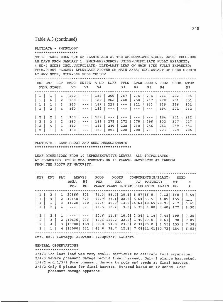
248
Table A.3 (continued)
PLOTDATA - PHENOLOGY ********************NOTES TAKEN WHEN 50% OF PLANTS ARE AT THE APPROPRIATE STAGE. DATES RECORDED AS DAYS FROM JANUARY 1 . EMRG=EMERGENCE; UNIFE=UNIFOLIATE FULLY EXPANDED;4 ND=4 NODES INCL.UNIFOLIATE; LLFE=LAST LEAF ON MAIN STEM FULLY EXPANDED; FFLW=FIRST FLOWER; LFLW=LAST FLOWER ON MAIN AXES; SDGR=START OF SEED GROWTH AT ANY NODE; MTUR=50% PODS YELLOW
REP ENT PLT EMRG UNIFE 4 ND LLFE FFLW LFLW PODO.5 P0D2 SDGR MTURFEHR STAGE: VO VI V4 R1 R2 R3 R4 R7
1 1 3 1 1 1 360 1 ----- 189 266 1 267 1 275 275 1 281 1 292 1 006 11 1 4 1 2 1 360 1 ----- 189 266 1 240 1 250 267 1 278 1 281 1 351 11 1 1 1 3 1 360 1 ----- 189 228 1 -----1 211 223 1 229 1 236 1 301 11 1 2 1 4 1 360 1 ----- 189 -----1 -----1 ----- -----1 194 1 201 1 242 1
1 2 2 1 1 1 360 1 ___ 189 ___ 1 ___ 1 ___ ___ 1 194 1 201 1 242 11 2 3 1 2 1 360 1 ----- 189 275 1 272 1 278 296 1 302 1 307 1 027 11 2 4 1 3 1 360 1 ----- 189 280 1 228 1 230 246 1 253 1 259 1 351 11 2 1 1 1 360 1 ----- 189 229 1 228 1 208 211 1 223 1 229 1 296 1
PLOTDATA - LEAF,SHOOT AND SEED MEASUREMENTS
LEAF DIMENSIONS FROM 10 REPRESENTATIVE LEAVES (ALL TRIFOLIATES)AT FLOWERING. OTHER MEASUREMENTS ON 10 PLANTS HARVESTED AT RANDOMFROM THE PLOTS AT MATURITY
REP ENT' PLT LEAVES PODS NODES COMPONENTS(G/PLANT) SEEDAREA WT PER PER AT MATURITY WT N
MM2 MG PLANT PLANT M. STEM PODS STEM GRAIN MG %
1 1 3 1 1 |20866| 503 7 4 . 0| 8 8 .7| 20 .51 8.871 5 6 .8 1 7 .121 168 1 8 .5 9 ]1 1 4 1 2 |19140| 670 72 .91 73 .11 22 .51 6 .6 4 15 3 .5 1 4 .051 155 1 11 1 1 1 3 1143201 660 6 9 .4| 45 .01 1 3 .6 1 1 4 .6 3 118 .691 28.91| 237 1 6 .4 1 ]1 1 2 1 4 1 — 1 ----- 23.51 1 0 .2 1 9.0| 3 .751 1 .081 7 .4 0 j 177 1 6 .90|
1 2 2 1 1 1 — 1 ___ 2 0 .6| 1 1 .6 1 10.21 3.34| 3 .1 4 1 7 .4 8 1 199 1 7 .2 6 ]1 2 3 1 2 |l9135 l 776 4 6 .6| 119.21 2 2 . 8 1 3.40| 3 7 .0 1 0.67| 98 1 7.89|1 2 4 1 3 |13700| 489 8 7 .oj 9 1 .0| 2 3 . o j 2 .331|75.0 1 1 .511 353 1 7.38|1 2 1 1 4 |13060| 631 4 3 . 6| 3 2 .7| 1 2 . 8 1 7.08|111 .O il 1 2 .7 2 ] 184 1 6.02|
E n t. n o . : l= B ra g g ; 2=E vans; 3 = J u p ite r ; 4= P adre .
GENERAL OBSERVATIONS * * * * * * * * * * * * * * * * * * * *
2 /4 / 3 The l a s t l e a f was v e r y s m a ll , d i f f i c u l t t o e s t im a te f u l l e x p a n s io n . 2 /4 / 3 S e v e re p h e a sa n t damage b e f o r e f i n a l h a r v e s t . O n ly 2 p la n t s h a r v e s t e d . 1 /4 / 2 and 1 /3 /1 Some p h ea sa n t damage t o p od s and s e e d s a t f i n a l h a r v e s t . 2 /3 / 2 O n ly 5 p la n t s f o r f i n a l h a r v e s t . W t/se e d b a se d on 10 s e e d s . Some
p h e a sa n t damage a p p a r e n t .

249
INFORMATION REQUIRED FOR DETAILED DATA ANALYSIS
SOYBEAN GENETIC COEFFICIENT NURSERIES
Table A.4 Soybean data from Haleakala Experiment Station, 17 h photoperiodtreatment.
INSTITUTENAME( INNAME) : IBSNATID (IN S T ID ): IB
RESEARCHER (S)NAME{RENAME) : R . OGOSHIID (R E SID ): RO
EXPERIMENTNAME {EXNAME) : SOYBEAN 17H (P3) DAYLENGTH STUDYID (EXPN): IDSS88H3
LOCATIONNAME: HALEAKALAID (LO C ): HK
SEEDINGYEAR (lYR) 1988DATE (ISOW;JULIAN DATE) 155SEED DEPTH (SDEPTH;CM) 4ESTABLISHED PLANT POPULATION (PLANTS; M -2) 3 3 .3ROW WIDTH (ROW;CM) 75
PHOTOPERIOD (HOURS) 17
IRRIGATION.JULIAN DATE OF J,TH IRRIGATION (JD AY (J))
AMOUNT OF WATER ADDED FOR J,TH IRRIGTION (AIRR(J);M M )
NITROGEN FERTILIZATIONJXHilAN DATE OF J,TH FERTILIZATION(JFDAY)
AMMOUNT OF NITROGEN ADDED FOR J,TH FERTILIZATION (AFERT;KG N/HA)0 _____________________________________________________________________________________________________
DEPTH OF INCORPORATION OF J,TH FERTILIZATION (D FE R T(J); CM,SURFACE APPLIED =1)
CODE NUMBER OF FERTILIZER TYPE FOR J,TH FERTILIZATION (UREA = 1;AMMONIUM NITRATE = 2;ANHYDRANE =3;CA AMMONIUM NITRATE = 4;M.NITRATE = 5)(IFTYPE(J))
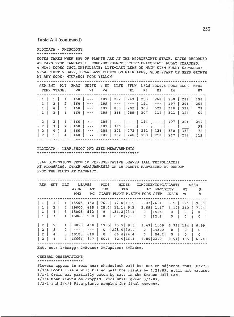
250
Table A.4 (continued)
PLOTDATA - PHENOLOGY * * * * * * * * * * * * * * * * * * * *
NOTES TAKEN WHEN 50% OF PLANTS ARE AT THE APPROPRIATE STAGE. DATES RECORDED AS DAYS FROM JANUARY 1 . EMRG=EMERGENCE; UNIFE=UNIFOLIATE FULLY EXPANDED;4 ND=4 NODES INCL.UNIFOLIATE; LLFE=LAST LEAF ON MAIN STEM FULLY EXPANDED; FFLW=FIRST FLOWER; LFLW=LAST FLOWER ON MAIN AXES; SDGR=START OF SEED GROWTH AT ANY NODE; MTUR=50% PODS YELLOW
REP ENT PLT EMRG UNIFE 4 ND LLFE FFLW LFLW PODO.5 P0D2 SDGR MTURFEHR STAGE: VO VI V4 R1 R2 R3 R4 R7
1 1 1 1 1 1 160 ___ 1 189 1 292 1 247 1 250 268 1 280 1 282 1 358 11 1 2 1 2 1 160 -----1 189 1 -----1 -------- 1 194 -----1 197 1 201 1 258 11 1 4 1 3 1 160 -----1 189 1 003 1 292 1 308 322 1 336 1 339 1 71 11 1 3 1 4 1 160 -----1 189 1 315 1 289 1 307 317 1 321 1 324 1 SO 1
1 2 2 1 1 1 160 -----1 189 1 -----1 -------- 1 194 ___ 1 197 1 201 1 249 11 2 11 3 1 2 1 160 ----1 189 1 336 1 1 1 1 1 93 11 2 !1 4 1 3 1 160 ----1 189 1 301 1 272 1 292 324 1 330 1 338 1 72 11 2 !1 1 1 4 1 160 ----1 189 1 292 1 246 1 250 258 1 267 1 272 1 312 1
PLOTDATA - LEAF,SHOOT AND SEED MEASUREMENTS
LEAP DIMENSIONS FROM 10 REPRESENTATIVE LEAVES (ALL TRIFOLIATES)AT FLOWERING. iOTHER MEASUREMENTS ON 10 PLANTS HARVESTED AT RANDOMFROM THE PLOTS AT MATURITY.
REP ENT■ PLT LEAVES PODS NODES COMPONENTS(G/PLANT) SEEDAREA WT PER PER AT MATURITY WT N
MM2 MG PLANT PLANT M.STEM PODS STEM GRAIN MG %
1 1 1 1 1 1155051 460 1 7 6 .6 1 7 2 .0 | 1 7 .0 1 5.07| 2 4 .1 1 5.55| 171 1 9-57|1 1 2 1 2 1196001 615 1 2 5 .2 ] 1 1 .1| 9 .3 1 3.69| 1.17| 4.19| 210 1 7.64|1 1 4 1 3 |15005| 512 1 0 | 1 3 1 .2 | 2 3 .1 1 0 16 5 .5 1 0 1 0 1 0 11 1 3 1 4 115068 1 538 1 0 1 6 0 .0 | 2 3 .8 1 0 16 2 .6 1 0 1 0 1 0 1
1 2 2 1 1 1 8890| 468 1 1 9 .5| 1 0 .7| 8 .8 1 3 .47| 1.05| 5.75| 194 1 6-99|1 2 3 1 2 1 — 1 ----1 0 12 2 8 .0 | 3 0 .0 1 0 11 4 3 .o j 0 1 0 1 0 11 2 4 1 3 Il8183| 618 1 0 1 6 6 . 8 1 2 4 .4 1 0 1 5 4 .2 0 1 0 1 0 11 2 1 1 4 1166661 547 1 5 0 . 6 1 4 2 .0 | 1 6 .4 1 6 .8 9 | 2 3 .0 1 9 .91| 165 1 6 .24|
E n t. n o . : l= B ra g g ; 2=E vans; 3 = J u p ite r ; 4= P adre .
GENERAL OBSERVATIONS * * * * * * * * * * * * * * * * * * * *
F lo w e rs a p p ea r in row s n ea r s h a d e c lo t h w a l l b u t n o t on a d ja c e n t row s ( 8 /2 7 ) . 1 /3 /4 Loolcs l i ) t e a w i l t ) c i l l e d h a l f th e p la n t s b y 1 /2 3 /8 9 , s t i l l n o t m atu re . 1 /1 / 1 G ra in was p a r t i a l l y e a te n b y r a t s in th e K rauss H a ll Lab.1 /3 / 4 M ost le a v e s on d ro p p e d . Pods s t i l l g r e e n 3 /3 /8 9 .1 /3 / 1 and 2 /4 /3 F iv e p la n t s sam pled f o r f i n a l h a r v e s t .

251
INFORMATION REQUIRED FOR DETAILED DATA ANALYSIS
SOYBEAN GENETIC COEFFICIENT NURSERIES
Table A. 5 Soybean data from Haleakala Experiment Station, 20 h photoperiodtreatment.
INSTITUTENAME( INNAME) : IBSNATID (IN S T ID ): IB
RESEARCHER (S)NAME(RENAME) : R . OGOSHIID (R E SID ): RO
EXPERIMENTNAME (EXNAME): SOYBEAN 2 OH (P4) DAYLENGTH STUDYID (EXPN): IDSS88H4
LOCATIONNAME: HALEAKALAID (L O C ): HK
SEEDINGYEAR (lYR ) 1988DATE (ISOW,-JULIAN DATE) 155SEED DEPTH (SDEPTH;CM) 4ESTABLISHED PLANT POPULATION (PLANTS,-M-2) 3 3 .3ROW WIDTH (ROW;CM) 75
PHOTOPERIOD (HOURS) 20
IRRIGATION.JULIAN DATE OF J,TH IRRIGATION (JD A Y (J))
AMOUNT OF WATER ADDED FOR J,TH IRRIGTION (AIRR(J),-MM)
NITROGEN FERTILIZATIONJULIAN DATE OF J,TH FERTILIZATION(JFDAY)
AMMOUNT OF NITROGEN ADDED FOR J,TH FERTILIZATION (AFERT,-KG N/HA)0 _________________________________________________________________________________________
DEPTH OF INCORPORATION OF J,TH FERTILIZATION (DFERT (J) ,-CM, SURFACE APPLIED =1)
CODE NUMBER OF FERTILIZER TYPE FOR J,TH FERTILIZATION (UREA = 1;AMMONIUM NITRATE = 2,-ANHYDRANE =3,-CA AMMONIUM NITRATE = 4;M.NITRATE = 5)(IFTYPE(J))
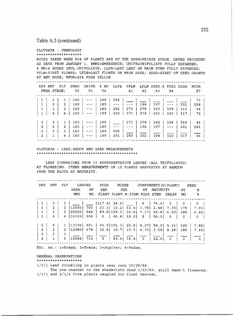
PLOTDATA - PHENOLOGY ********************NOTES TAKEN WHEN 50% OF PLANTS ARE AT THE APPROPRIATE STAGE. DATES RECORDED AS DAYS FROM JANUARY 1 . EMRG=EMERGENCE; UNIFE=UNIFOLIATE FULLY EXPANDED;4 ND=4 NODES INCL.UNIFOLIATE; LLFE=LAST LEAF ON MAIN STEM FULLY EXPANDED; FFLW=FIRST FLOWER; LFLW=LAST FLOWER ON MAIN AXES; SDGR=START OF SEED GROWTH AT ANY NODE; MTUR=50% PODS YELLOW
252
Table A. 5 (continued)
REP ENT PLT EMRG UNIFE 4 ND LLFE FFLW LFLW PODO.5 P0D2 SDGR MTURFEHR STAGE: VO VI V4 R1 R2 R3 R4 R7
1 1 3 1 1 1 160 1 --- 1 189 1 006 1 1 1 73 11 1 2 1 2 1 160 1 --- 1 189 1 ----- --- 1 194 197 1 ----- 201 1 2581 1 1 1 3 1 160 1 --- 1 189 1 292 270 1 278 303 1 308 310 441 1 4 1 4 1 160 1 --- 1 189 1 292 271 1 278 303 1 310 317 1 72 I
1 2 4 1 1 1 160 1 __ 1 189 1 271 1 279 302 1 336 345 1 44 11 2 2 1 2 1 160 1 - - - 1 189 1 . . . -----1 194 197 1 ----- 201 1 261 11 2 3 I 3 1 160 1 -----1 189 1 005 1 , 1 1 11 2 1 1 4 1 160 1 -----1 189 1 291 289 1 302 308 1 310 317 1 44 1
PLOTDATA - LEAF,SHOOT AND SEED MEASUREMENTS
LEAF DIMENSIONS FROM 10 REPRESENTATIVE LEAVES (ALL TRIFOLIATES)AT FLOWERING. OTHER MEASUREMENTS ON 10 PLANTS HARVESTED AT RANDOMFROM THE PLOTS AT MATURITY.
REP ENT PLT LEAVES PODS NODES COMPONENTS(G/PLANT) SEEDAREA WT PER PER AT MATURITY WT N
MM2 MG PLANT PLANT M.STEM PODS STEM GRAIN MG %
1 1 3 1 1 1 1 117.41 2 4 . 6 1 1 0 1 7 4 .4| 0 1 0 1 0 11 1 2 1 2 I 126601 703 1 23 .31 12.21 1 0 .4| 3 .7 8 1 2 .481 7 .351 175 1 7 .031j 1 1 1 3 1 201001 542 1 6 9 .6| 1 3 6 .3 1 2 2 . 8 1 7 .1 7 1 56 .81 6 .301 185 1 6.85|1 1 4 1 ^ 1141941 559 1 0 1 6 6 .8 1 1 9 .3| 0 1 5 0 .0| 0 1 0 1 0 1
1 2 4 1 1 1131941 461 1 4 1 .9 | 1 0 1 .3 | 2 5 .8 1 4 .3 7 1 5 4 .2| 5 .411 190 1 7.89|1 2 2 1 2 |12980| 674 1 32 .51 1 6 .7| 13.31 4 .7 6 1 3.58| 8 .2 8 1 180 1 7.45|1 2 3 1 3 1 1 1 1 , 1 1 1 1 1 11 2 1 1 4 1155881 714 1 0 1 8 9 .4j 18 .4 1 0 1 5 2 .0| 0 1 0 1 0 1
E n t. n o . : l= B ra g g ; 2=E vans; 3 = J u p ite r ; 4= P adre .
GENERAL OBSERVATIONS * * * * * * * * * * * * * * * * * * * *
1 /3 / 1 L e a f c r i n k l i n g on p la n t s n ea r co rn 1 0 /2 8 /8 8 .The row n e a r e s t t o th e s h a d e c lo t h d ie d 1 /2 3 /8 9 , s t i l l h a s n 't f l o w e r e d .
1 /3 / 1 and 2 /1 / 4 F iv e p la n t s sam pled f o r f i n a l h a r v e s t .

253
INFORMATION REQUIRED FOR DETAILED DATA ANALYSIS
SOYBEAN GENETIC COEFFICIENT NURSERIES
Table A.6 Soybean data from Kuiaha Experiment Site, control photoperiodtreatment.
INSTITUTENAME(INNAME): ID (IN S T ID ):
IBSNATIB
RESEARCHER (S)NAME(RENAME): ID (R E SID ):
R.OGOSHI RO
EXPERIMENTNAME (EXNAME): ID (EXPN):
SOYBEAN CONTROL (PO) DAYLENGTH STUDY IDSS88K0
LOCATIONNAME:ID (LO C ):
KUIAHAKU
SEEDINGYEAR (lYR ) 1988DATE (ISOW;JULIAN DATE) 155SEED DEPTH (SDEPTH;CM) 4ESTABLISHED PLANT POPULATION (PLANTS;M-2) 3 3 .3 ROW WIDTH (ROW;CM) 75
PHOTOPERIOD (HOURS) NATURAL
IRRIGATION.JULIAN DATE OF J,TH IRRIGATION (JD A Y (J))
AMOUNT OF WATER ADDED FOR J,TH IRRIGTION (AIRR(J);M M )
NITROGEN FERTILIZATIONJULIAN DATE OF J,TH FERTILIZATION(JFDAY)
AMMOUNT OF NITROGEN ADDED FOR J,TH FERTILIZATION (AFERT;KG N/HA)0 _______________________________________________________________________________________________
DEPTH OF INCORPORATION OF J,TH FERTILIZATION (D FE R T(J); CM,SURFACE APPLIED =1)
CODE NUMBER OF FERTILIZER TYPE FOR J,TH FERTILIZATION (UREA = 1;AMMONIUM NITRATE = 2;ANHYDRANE =3;CA AMMONIUM NITRATE = 4;M.NITRATE = 5)(IFTYPE(J))
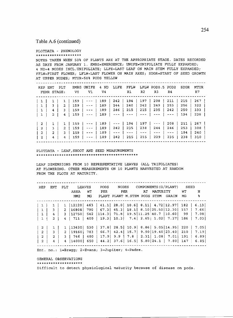
254
Table A.6 (continued)
PLOTDATA - PHENOLOGY * * * * * * * * * * * * * * * * * * * *
NOTES TAKEN WHEN 50% OF PLANTS ARE AT THE APPROPRIATE STAGE. DATES RECORDED AS DAYS FROM JANUARY 1 . EMRG=EMERGENCE; UNIFE=UNIFOLIATE FULLY EXPANDED;4 ND=4 NODES INCL.UNIFOLIATE; LLFE=LAST LEAF ON MAIN STEM FULLY EXPANDED; FFLW=FIRST FLOWER; LFLW=LAST FLOWER ON MAIN AXES; SDGR=START OF SEED GROWTH AT UPPER NODES; MTUR=50% PODS YELLOW
REP ENT PLT EMRG UNIFE 4 ND LLFE FFLW LFLW POD0.5 P0D2 SDGR MTURFEHR STAGE: VO VI V4 R1 R2 R3 R4 R7
1 1 1 1 1 1 159 1 - - - 1 189 1 242 1 194 1 197 208 1 211 1 215 1 267 11 1 3 1 2 1 159 1 - - - 1 189 1 244 1 240 1 242 249 1 253 1 256 1 322 11 1 4 1 3 1 159 1 - - - 1 189 1 246 1 215 1 215 235 1 242 1 250 1 333 11 1 2 1 4 1 159 1 - - - 1 189 1 — 1 -----1 . . . . . . 1 . . . 1 194 1 236 1
1 2 1 1 1 1 159 1 - - - 1 189 1 — 1 194 1 197 . . . 1 208 1 211 1 267 11 2 3 1 2 1 159 1 - - - 1 189 1 242 1 235 1 238 244 1 246 1 253 1 308 11 2 2 1 3 1 159 1 - - - 1 189 1 . . . 1 -----1 ----- ----- 1 -----1 194 1 240 11 2 4 1 4 1 159 1 ----- 1 189 1 242 1 215 1 215 229 1 235 1 238 1 310 1
PLOTDATA - LEAF,SHOOT AND SEED MEASUREMENTS
LEAF DIMENSIONS FROM 10 REPRESENTATIVE LEAVES (ALL TRIFOLIATES)AT FLOWERING. OTHER MEASUREMENTS ON 10 PLANTS HARVESTED AT RANDOMFROM THE PLOTS AT MATURITY.
REP ENT' PLT LEAVES PODS NODES COMPONENTS(G/PLANT) SEEDAREA WT PER PER AT MATURITY WT N
MM2 MG PLANT PLANT M.STEM PODS STEM GRAIN MG %
1 1 1 1 1 1 1121201 463 1 4 1 . l| 2 8 .0| 1 0 . 6 1 8 . I l l j 4 .7 2 l l 2 . 9 7 l 182 1 6 .1 3 11 1 1 3 1 2 1168081 790 1 6 7 .3| 4 5 .3 1 1 8 . l| 8 .1 0 2 5 .5 0 l l2 .3 0 | 157 1 7 . 66 11 1 1 4 1 3 1127501 542 |114.3| 7 1 .8| 19 .51 1 1 .2 5 |40.7 |10.60| 99 1 7.08|1 1 1 2 1 4 1 711 1 400 I 1 9 .3| 1 0 .3 1 7 .41 2 .6 5 1 1 .02| 7 .37| 186 1 7 .0 3 1
1 2 1 1 1 1 1Il3630| 530 1 37 .81 2 8 .5| 10.91 8 .8 6 1 5 .0 5 1 1 4 .9 5 1 220 1 7 .0511 2 1 3 1 2 119160| 783 1 6 6 .7| 4 2 .4| 15 .71 9 .9 0 1 1 9 .4 0 1 2 3 .4 0 1 210 1 7 .1911 2 1 2 1 3 11 746 1 400 1 1 7 .9| 9 .9 1 7 .8 1 2 .3 1 1 1 .08| 7 .01| 191 1 6 .8911 2 1 4 1 4 1|14000| 650 1 4 4 .2| 3 7 .6| 1 6 .5| 5 .8 0 |24.1 1 7 .80| 147 1 6 .851
E n t. n o . : l= B ra g g ; 2=E vans; 3 = J u p ite r ; 4= P adre .
GENERAL OBSERVATIONS * * * * * * * * * * * * * * * * * * * *
D i f f i c u l t t o d e t e c t p h y s i o l o g i c a l m a tu r ity b e ca u s e o f d i s e a s e on p o d s .
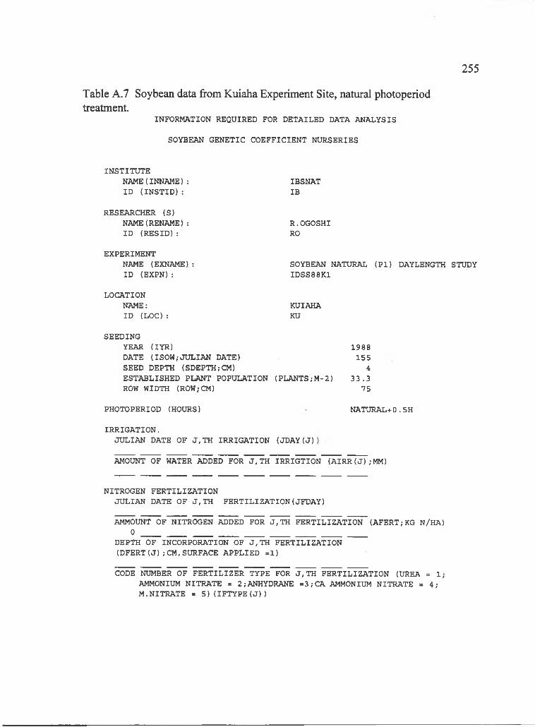
255
INFORMATION REQUIRED FOR DETAILED DATA ANALYSIS
SOYBEAN GENETIC COEFFICIENT NURSERIES
Table A.7 Soybean data from Kuiaha Experiment Site, natural photoperiodtreatment.
INSTITUTENAME(INNAME): ID (IN S T ID ):
IBSNATIB
RESEARCHER (S)NAME(RENAME): ID (R E SID ):
R.OGOSHI RO
EXPERIMENTNAME (EXNAME): ID (EXPN):
SOYBEAN NATURAL (P I) DAYLENGTH STUDY IDSS88K1
LOCATIONNAME:ID (LO C ):
KUIAHAKU
SEEDINGYEAR (lYR) 1988DATE (ISOW;JULIAN DATE) 155SEED DEPTH (SDEPTH;CM) 4ESTABLISHED PLANT POPULATION (PLANTS;M-2) 3 3 .3 ROW WIDTH (ROW;CM) 75
PHOTOPERIOD (HOURS) NATURAL+0.5H
IRRIGATION.JULIAN DATE OF J,TH IRRIGATION (JDAY(J)
AMOUNT OF WATER ADDED FOR J,TH IRRIGTION (AIRR(J);M M )
NITROGEN FERTILIZATIONJULIAN DATE OF J,TH FERTILIZATION(JFDAY)
AMMOUNT OF NITROGEN ADDED FOR J,TH FERTILIZATION (AFERT;KG N/HA)0 _________________________________________________________
DEPTH OF INCORPORATION OF J,TH FERTILIZATION (D FE R T(J); CM,SURFACE APPLIED =1)
CODE NUMBER OF FERTILIZER TYPE FOR J,TH FERTILIZATION (UREA = 1;AMMONIUM NITRATE = 2;ANHYDRANE =3;CA AMMONIUM NITRATE = 4;M.NITRATE = 5)(IFTYPE(J))
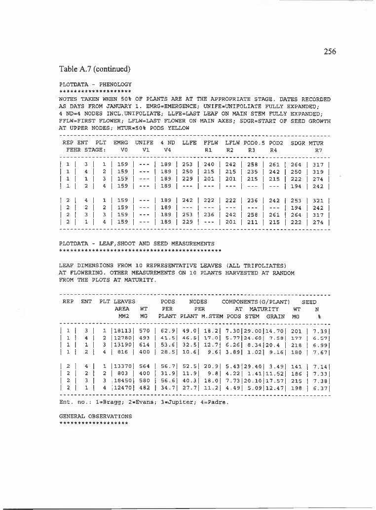
256
Table A.7 (continued)
PLOTDATA - PHENOLOGY ********************NOTES TAKEN WHEN 50% OF PLANTS ARE AT THE APPROPRIATE STAGE. DATES RECORDED AS DAYS FROM JANUARY 1 . EMRG=EMERGENCE; UNIFE=UNIFOLIATE FULLY EXPANDED;4 ND=4 NODES INCL.UNIFOLIATE; LLFE=LAST LEAF ON MAIN STEM FULLY EXPANDED; FFLW=FIRST FLOWER; LFLW=LAST FLOWER ON MAIN AXES; SDGR=START OF SEED GROWTH AT UPPER NODES; MTUR=50% PODS YELLOW
REP ENT PLT EMRG UNIFE 4 ND LLFE FFLW LFLW PODO. 5 P0D2 SDGR MTURFEHR STAGE: VO VI V4 R1 R2 R3 R4 R7
1 1 3 1 1 1 5 9 1 ____ 1 8 9 ] 253 ] 24 0 ] 2 4 2 ] 2 5 8 ] 2 6 1 ] 2 6 4 3 1 7 ]I 1 4 1 2 1 5 9 1 -------- 1 8 9 1 2 5 0 j 2 1 5 j 2 1 5 1 2 3 5 j 2 4 2 j 2 5 0 3 1 9 jI 1 1 1 3 1 5 9 I -------- 1 8 9 ] 2 2 9 j 2 0 1 j 2 0 1 j 2 1 5 ] 2 1 5 j 2 2 2 2 7 4 jI 1 2 1 4 1 5 9 I -------- 1 8 9 j -----1 -----1 -----1 --------] ------------- 1 194 2 4 2 j
1 2 4 1 1 1 5 9 1 ___ 1 8 9 ] 2 4 2 ] 2 2 2 ] 2 2 2 ] 23 6 ] 2 4 2 ] 2 5 3 3 2 1 ]1 2 2 1 2 1 5 9 I -------- 1 8 9 ] -----1 -----J -----1 --------1 -------------I 194 2 4 2 ]I 2 3 I 3 1 5 9 1 -------- 1 8 9 j 253 j 23 6 j 2 4 2 j 25 8 j 2 6 1 ] 2 6 4 3 1 7 j1 2 1 1 4 1 5 9 I -------- 1 8 9 ] 22 9 j -----1 2 0 1 j 2 1 1 j 2 1 5 ] 2 2 2 2 7 4 j
PLOTDATA - LEAF,SHOOT AND SEED MEASUREMENTS
LEAF DIMENSIONS FROM 10 REPRESENTATIVE LEAVES (ALL TRIFOLIATES)AT FLOWERING. OTHER MEASUREMENTS ON 10 PLANTS HARVESTED AT RANDOMFROM THE PLOTS AT MATURITY.
REP ENT PLT LEAVES PODS NODES COMPONENTS(G/PLANT) SEEDAREA WT PER PER AT MATURITY WT N
MM2 MG PLANT PLANT M.STEM PODS STEM GRAIN MG %
1 1 3 1 1 11181131 570 6 2 . 9 ] 4 9 . 0 ] 18 . 2 ] 7 . 3 0 ] 2 9 . 0 0 ] 1 4 . 7 0 ] 20 1 7 . 3 9 ]1 1 4 1 2 112 78 01 4 93 4 1 . 5 ] 4 6 . 5 ] 1 7 . 0 ] S . 7 7 ] 2 4 . G 0 7 . 5 8 1 7 7 6 . 57 j1 1 1 1 3 11 3 1 9 0 I G14 53 .6 j 3 2 . 5 ] 1 2 . 7 ] 6 . 2 6 ] 8 . 3 4 ] 2 0 . 4 ] 2 1 8 6 . 9 9 ]1 1 2 1 4 11 816 1 4 0 0 2 8 . 5 ] 1 0 . 6 ] 9 . 6 ] 3 . 8 9 ] 1 . 0 2 ] 9 . 1 6 ] 180 7 . 6 7 ]
1 2 4 1 1 i1 1 3 3 7 0 ] 564 5 6 . 7 ] 5 2 . 5 ] 2 0 . 9 ] 5 . 4 3 ] 2 9 . 4 0 ] 3 . 4 9 ] 141 7 . 1 4 )I 2 2 1 2 11 803 ] 40 0 3 1 . 9 ] 1 1 . 9 ] 9 . 8 ] 4 . 2 2 j 1 . 4 1 ] 1 1 . 5 2 ] 186 7 . 3 3 ]1 2 3 1 3 ] 1 8 4 5 0 ] 580 5 6 . 6 ] 4 0 . 3 ] 1 8 . 0 ] 7 . 7 3 ] 2 0 . 1 0 ] 1 7 . 5 7 ] 2 1 5 7 . 3 8 ]1 2 1 1 4 1 12 47 0] 48 2 3 4 . 7 ] 2 7 . 7 ] 1 1 . 2 ] 4 . 4 9 ] 5 . 0 9 ] 1 2 . 4 7 ] 198 6 . 3 7 ]
E n t. n o . : l= B ra g g ; 2=E vans; 3 = J u p ite r ; 4= P adre .
GENERAL OBSERVATIONS * * * * * * * * * * * * * * * * * * *

257
Table A. 8 Soybean data from Kuiaha Experiment Site, 14 h photoperiod treatment.INFORMATION REQUIRED FOR DETAILED DATA ANALYSIS
SOYBEAN GENETIC COEFFICIENT NURSERIES
INSTITUTENAME( INNAME) : IBSNATID (IN S T ID ): IB
RESEARCHER (S)NAME(RENAME): R . OGOSHIID (R E SID ): RO
EXPERIMENTNAME (EXNAME): SOYBEAN 14H (P2) DAYLENGTH STUDYID (EXPN): IDSS88K2
LOCATIONNAME: KUIAHAALAID (LO C ): KU
SEEDINGYEAR (lYR) 1988DATE (ISOW;JXmiAN DATE) 155SEED DEPTH (SDEPTH;CM) 4ESTABLISHED PLANT POPULATION (PLANTS;M-2) 3 3 .3 ROW WIDTH (ROW;CM) 75
PHOTOPERIOD (HOURS) 14
IRRIGATION.JULIAN DATE OF J,TH IRRIGATION (JD AY (J))
AMOUNT OF WATER ADDED FOR J,TH IRRIGTION (AIRR(J);M M )
NITROGEN FERTILI2ATI0NJULIAN DATE OF J,TH FERTILIZATION(JFDAY)
AMMOUNT OF NITROGEN ADDED FOR J,TH FERTILIZATION (AFERT;KG N/HA)0 _______________________________________________________________________________________________
DEPTH OF INCORPORATION OF J,TH FERTILIZATION (D FE R T(J); CM,SURFACE APPLIED =1)
CODE NUMBER OF FERTILIZER TYPE FOR J,TH FERTILIZATION (UREA = 1;AMMONIUM NITRATE = 2;ANHYDRANE =3;CA AMMONIUM NITRATE = 4;M.NITRATE = 5)(IFTYPE(J))
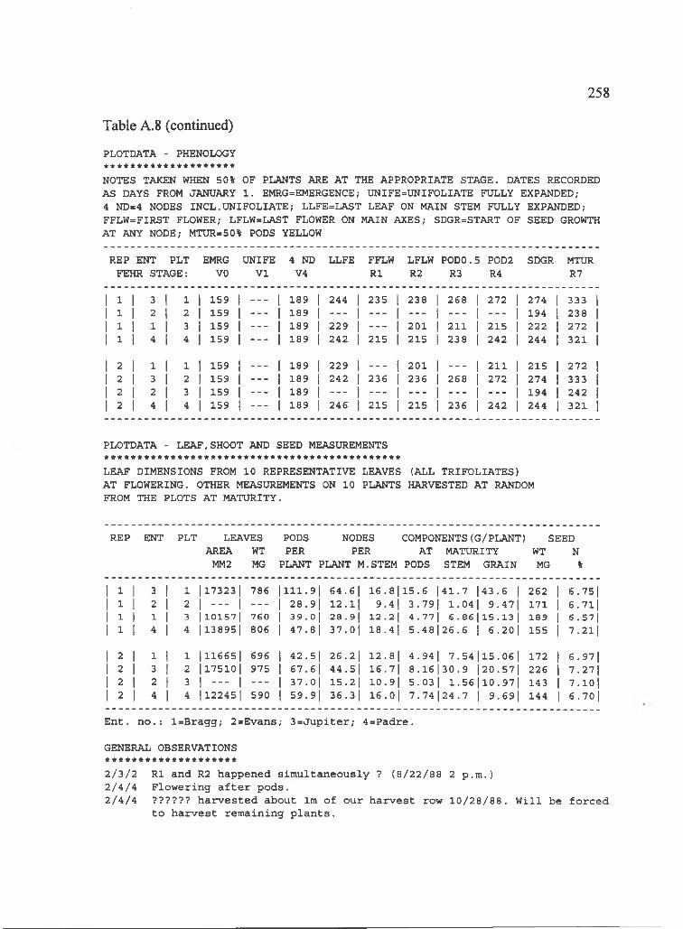
258
Table A. 8 (continued)
PLOTDATA - PHENOLOGY * * * * * * * * * * * * * * * * * * * *
NOTES TAKEN WHEN 50% OF PLANTS ARE AT THE APPROPRIATE STAGE. DATES RECORDED AS DAYS FROM JANUARY 1 . EMRG=EMERGENCE; UNIFE=UNIFOLIATE FULLY EXPANDED;4 ND=4 NODES INCL. UNIFOLIATE; LLFE=LAST LEAF ON MAIN STEM FULLY EXPANDED; FFLW=FIRST FLOWER; LFLW=LAST FLOWER ON MAIN AXES; SDGR=START OF SEED GROWTH AT ANY NODE; MTUR=50% PODS YELLOW
REP ENT PLT EMRG UNIFE 4 ND LLFE FFLW LFLW PODO.5 P0D2 SDGR MTURFEHR STAGE: VO VI V4 R1 R2 R3 R4 R7
1 1 3 1 1 1 359 1 ___ 1 189 1 244 235 1 238 268 1 272 1 274 1 333 11 1 2 1 3 1 359 1 ----- 1 389 1 ----- -----1 ----- -----1 -------- j 194 I 238 11 1 1 1 3 1 359 1 ----- 1 389 1 229 -----1 201 211 1 215 1 222 1 272 11 1 4 1 4 1 359 1 ----- 1 389 1 242 215 1 215 238 1 242 1 244 1 321 1
1 3 1 1 1 1 359 1 ___ 1 389 1 229 ___ 1 201 - - - 1 211 1 215 1 272 1I 3 3 1 3 1 359 1 ----- 1 389 I 242 236 1 236 268 1 272 1 274 1 333 j1 3 2 1 3 1 359 1 ----- 1 389 1 ----- -----1 ----- -----1 -------- 1 194 1 242 jI 3 4 1 4 1 359 1 ----- I 389 1 246 215 1 215 236 1 242 1 244 1 321 j
PLOTDATA - LEAF,SHOOT AND SEED MEASUREMENTS
LEAF DIMENSIONS FROM 10 REPRESENTATIVE LEAVES (ALL TRIFOLIATES)AT FLOWERING. OTHER MEASUREMENTS ON 10 PLANTS HARVESTED AT RANDOMFROM THE PLOTS AT MATURITY •
REP ENT' PLT LEAVES PODS NODES COMPONENTS(G/PLANT) SEEDAREA WT PER PER AT MATURITY WT N
MM2 MG PLANT PLANT M.STEM PODS STEM GRAIN MG %
1 1 3 1 1 1173231 786 |331.9| 6 4 .6 1 1 6 .8 1 1 5 .6 |41 .7 143 .6 1 262 6 .7511 3 2 1 2 1 — 1 ----- 1 2 8 .9| 1 2 .1 1 9.41 3 .79 1 1 .0 4 j 9 .4 7 171 6 . 7 l jI 1 1 1 3 11 0 1 5 7 1 7 60 1 3 9 - 0 | 28 . 9 1 12 .21 4 . 7 7 ] 6 . 8 6 ] 1 5 . 1 3 ] 1 89 6 .5 7 j1 1 4 1 4 113895| 806 1 4 7 . 8| 3 7 .0 1 38.41 5 .4 8 | 2 6 .6 1 6 .2 o j 1 5 5 7.211
1 3 1 1 1 111665 1 696 1 42 .51 2 6 .2 1 32 .81 4 .9 4 1 7 .5 4 | l5 .0 6 l 172 6 .9 7 11 2 3 1 2 117510 1 975 1 6 7 .6| 44 .51 36 .71 8 .1 6 | 30 .9 |20.57| 226 7 .2711 2 2 1 3 1 — 1 ----- 1 3 7 . o j 1 5 .2 1 30.91 5 .0 3 1 1 .5 6 j l 0 . 9 7 j 143 7 .1 0 ]1 3 4 1 4 112245 I 590 1 5 9 . s j 3 6 .3 1 1 6 .0| 7 .7 4 |24.7 1 9 .6 9 j 144 6 . 70 I
E n t. n o . : l= B ra g g ; 2=E vans; 3 = J u p it e r ; 4= P adre .
GENERAL OBSERVATIONS * * * * * * * * * * * * * * * * * * * *
I / I l l R1 and R2 happened s im u lta n e o u s ly ? ( 8 /2 2 /8 8 2 p .m .)2 / i / i F lo w e r in g a f t e r p o d s .2 /4 / 4 ? ? ? ? ? ? h a r v e s te d a b ou t Im o f o u r h a r v e s t row 1 0 /2 8 /8 8 . W il l be f o r c e d
t o h a r v e s t rem a in in g p l a n t s .

259
Table A.9 Soybean data from Kuiaha Experiment Site, 17 h photoperiod treatment.INFORMATION REQUIRED FOR DETAILED DATA ANALYSIS
SOYBEAN GENETIC COEFFICIENT NURSERIES
INSTITUTENAME( INNAME) : IBSNATID (IN S T ID ): IB
RESEARCHER (S)NAME(RENAME) : R . OGOSHIID (R E SID ): RO
EXPERIMENTNAME (EXNAME): SOYBEAN 17H (P3) DAYLENGTH STUDYID (EXPN): IDSS88K3
LOCATIONNAME: KUIAHAID (LO C ): KU
SEEDINGYEAR (lYR ) 1988DATE (ISOW;JULIAN DATE) 155SEED DEPTH (SDEPTH;CM) 4ESTABLISHED PLANT POPULATION (PLANTS;M-2) 3 3 .3 ROW WIDTH (ROW;CM) 75
PHOTOPERIOD (HOURS) 17
IRRIGATION.JULIAN DATE OF J,TH IRRIGATION (JD A Y (J))
AMOUNT OF WATER ADDED FOR J,TH IRRIGTION (AIRR(J);M M )
NITROGEN FERTILIZATIONJULIAN DATE OF J,TH FERTILIZATION(JFDAY)
AMMOUNT OF NITROGEN ADDED FOR J,TH FERTILIZATION (AFERT;KG N/HA)0 _______________________________________________________________________________________________
DEPTH OF INCORPORATION OF J,TH FERTILIZATION (D FE R T(J); CM,SURFACE APPLIED =1)
CODE NUMBER OF FERTILIZER TYPE FOR J,TH FERTILIZATION (UREA = 1;AMMONIUM NITRATE = 2;ANHYDRANE =3;CA AMMONIUM NITRATE = 4;M.NITRATE = 5)(IFTYPE(J))
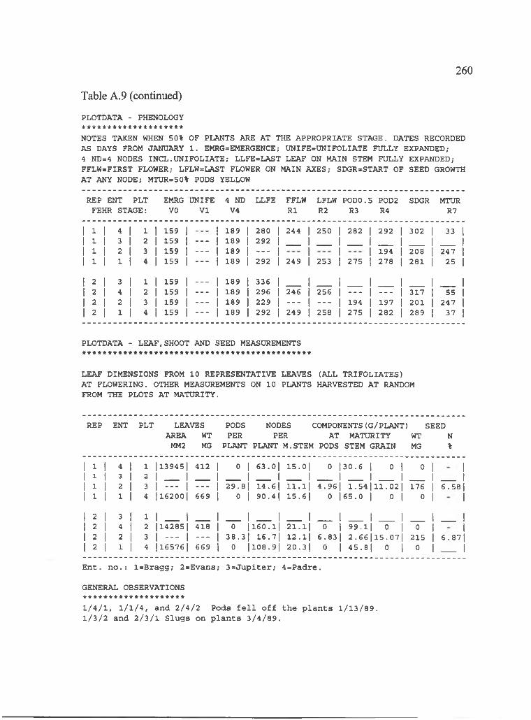
260
Table A.9 (continued)
PLOTDATA - PHENOLOGY ********************NOTES TAKEN WHEN 50% OF PLANTS ARE AT THE APPROPRIATE STAGE. DATES RECORDED AS DAYS FROM JANUARY 1 . EMRG=EMERGENCE; UNIFE=UNIFOLIATE FULLY EXPANDED;4 ND=4 NODES INCL.UNIFOLIATE; LLFE=LAST LEAF ON MAIN STEM FULLY EXPANDED; FFLW-FIRST FLOWER; LFLW=LAST FLOWER ON MAIN AXES; SDGR=START OF SEED GROWTH AT ANY NODE; MTUR=50% PODS YELLOW
REP ENT PLT EMRG UNIFE 4 ND LLFE FFLW LFLW PODO.!5 P0D2 SDGR MTURFEHR STAGE: VO VI V4 R1 R2 R3 R4 R7
1 1 4 1 1 1 159 1 ----- 189 1 280 1 244 1 250 1 282 1 292 1 302 1 33 11 1 3 1 2 1 159 1 ----- 189 1 292 1 1 1 1 1 11 1 2 1 3 1 159 1 ----- 189 1 -----1 1 194 1 208 1 247 11 1 1 1 4 1 159 1 ----- 189 1 292 1 249 1 253 1 275 1 278 1 281 1 25 1
1 2 3 1 1 1 159 1 __ 189 1 336 1 1 1 1 1 11 2 4 1 2 1 159 1 ----- 189 1 296 1 246 1 256 1 - - - 1 -----1 317 1 55 11 2 2 1 3 1 159 1 ----- 189 1 229 1 -----1 - - - 1 194 1 197 1 201 1 2471 2 1 1 4 1 159 1 ----- 189 1 292 1 249 1 258 1 275 1 282 1 289 1 37 1
PLOTDATA - LEAF,SHOOT AND SEED MEASUREMENTS
LEAF DIMENSIONS FROM 10 REPRESENTATIVE LEAVES (ALL TRIFOLIATES)AT FLOWERING. OTHER MEASUREMENTS ON 10 PLANTS HARVESTED .AT RANDOMFROM THE PLOTS AT MATURITY.
REP ENT' PLT LEAVES PODS NODES COMPONENTS(G/PLANT) SEEDAREA WT PER PER AT MATURITY WT N
MM2 MG PLANT PLANT M. STEM PODS STEM GRAIN MG %
1 1 4 1 1 |13945| 412 0 1 6 3 .0| 1 5 .0| 0 130 .6 1 0 1 0 1 11 1 3 1 2 1 1 1 1 1 1 1 1 , , 11 1 2 1 3 1 — 1 ----- 2 9 .8| 1 4 .6 1 11 .11 4.96| 1 .5 4 | 1 1 .0 2 | 176 1 6.58|1 1 1 1 4 1162001 669 0 1 9 0 .4| 1 5 .6| 0 |65.0 1 0 1 0 1 1
1 2 3 1 1 1 1 1 1 1 1 1 1 11 2 4 1 2 |14285| 418 0 11 6 0 .l| 2 1 . 1| 0 1 9 9 .1 1 0 1 0 11 2 2 1 3 1 — 1 ----- 3 8 .3| 16 . 7 1 1 2 .1| 6.83| 2 .6 6 |15.07| 215 1 6 .8 7 ]1 2 1 1 4 1165761 669 0 |108.9| 2 0 .3| 0 1 4 5 .8 1 0 1 0 1 1
E n t. n o . : l= B ra g g ; 2=E vans; 3 = J u p it e r ; 4= P adre .
GENERAL OBSERVATIONS ********************1 / 4 / 1 , 1 /1 / 4 , and 2 /4 / 2 Pods f e l l o f f th e p la n t s 1 /1 3 /8 9 . 1 /3 /2 and 2 /3 / 1 S lu g s on p la n t s 3 /4 /8 9 .
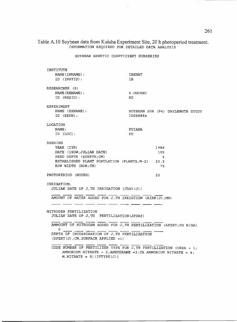
Table A. 10 Soybean data from Kuiaha Experiment Site, 20 h photoperiod treatment.INFORMATION REQUIRED FOR DETAILED DATA ANALYSIS
SOYBEAN GENETIC COEFFICIENT NURSERIES
261
INSTITUTENAME(INNAME): IBSNATID (IN S T ID ): IB
RESEARCHER (S)NAME(RENAME) : R . OGOSHIID (R E SID ): RO
EXPERIMENTNAME (EXNAME): SOYBEAN 2 OH (P4) DAYLENGTH STUDYID (EXPN): IDSS88K4
LOCATIONNAME: KUIAHAID (LO C ): KU
SEEDINGYEAR (lYR) 1988DATE (ISOW;JULIAN DATE) 155SEED DEPTH (SDEPTH;CM) 4ESTABLISHED PLANT POPULATION (PLANTS;M-2) 3 3 .3 ROW WIDTH (ROW;CM) 75
PHOTOPERIOD (HOURS) 20
IRRIGATION.JULIAN DATE OF J,TH IRRIGATION (JD AY (J))
AMOUNT OF WATER ADDED FOR J,TH IRRIGTION (AIRR(J);M M )
NITROGEN FERTILIZATIONJULIAN DATE OF J,TH FERTILIZATION(JFDAY)
AMMOUNT OF NITROGEN ADDED FOR J,TH FERTILIZATION (AFERT;KG N/HA)0 _________________________________________________________
DEPTH OF INCORPORATION OF J,TH FERTILIZATION (D FE R T(J); CM,SURFACE APPLIED =1)
CODE NUMBER OF FERTILIZER TYPE FOR J,TH FERTILIZATION (UREA = 1;AMMONIUM NITRATE = 2;ANHYDRANE =3;CA AMMONIUM NITRATE = 4;M.NITRATE = 5)(IFTYPE(J))
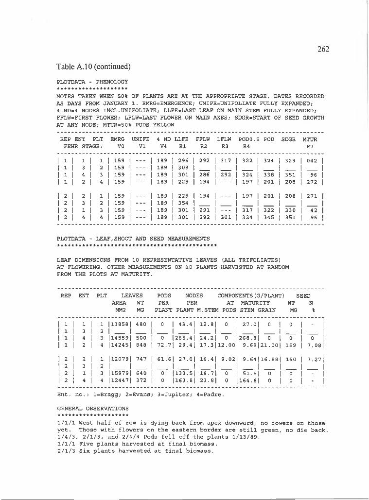
262
Table A. 10 (continued)
PLOTDATA - PHENOLOGY * * * * * * * * * * * * * * * * * * * *
NOTES TAKEN WHEN 50% OF PLANTS ARE AT THE APPROPRIATE STAGE. DATES RECORDED AS DAYS FROM JANUARY 1 . EMRG=EMERGENCE; UNIFE=UNIFOLIATE FULLY EXPANDED;4 ND=4 NODES INCL.UNIFOLIATE; LLFE=LAST LEAF ON MAIN STEM FULLY EXPANDED; FFLW=FIRST FLOWER; LFLW=LAST FLOWER ON MAIN AXES; SDGR=START OF SEED GROWTH AT ANY NODE; MTUR=50% PODS YELLOW
REP ENT PLT EMRG UNIFE 4 ND LLFE FFLW :LFLW PODO.15 POD SDGR MTURFEHR STAGE: VO VI V4 R1 R2 R3 R4 R7
1 1 1 1 1 1 159 1 ___ 1 189 296 1 292 1 317 322 324 1 329 1 042 11 1 3 1 2 1 159 1 -----1 189 308 1 1 1 , 11 1 4 1 3 1 159 1 -----1 189 301 1 286 1 292 324 338 1 351 1 96 11 1 2 1 4 1 159 1 -----1 189 229 1 194 1 ----- 197 201 1 208 1 272 1
1 2 2 1 1 1 159 1 ___ 1 189 229 1 194 1 ----- 197 201 1 208 1 271 11 2 3 1 2 1 159 1 -----1 189 354 1 1 1 11 2 1 1 3 1 159 1 -----1 189 301 1 291 1 ----- 317 322 1 330 1 42 11 2 4 1 4 1 159 1 -----1 189 301 1 292 1 301 324 345 1 351 1 56 1
PLOTDATA - LEAF,SHOOT AND SEED MEASUREMENTS* * * * * * * * * * * * * * * * * * * * * * * * * * * * * * * * * * * * * * * * * * * * *
LEAF DIMENSIONS FROM 10 REPRESENTATIVE LEAVES (ALL TRIFOLIATES)AT FLOWERING. 'OTHER MEASUREMENTS ON 10 PLANTS HARVESTED AT RANDOMFROM THE PLOTS AT MATURITY.
REP ENT' PLT LEAVES PODS NODES COMPONENTS(G/PLANT) SEEDAREA WT PER PER AT MATURITY WT N
MM2 MG PLANT PLANT M.STEM PODS STEM GRAIN MG %
1 1 1 1 1 1 |13858| 480 1 0 1 43 .41 1 2 .8 1 0 1 2 7 .0 1 0 0 1 - 11 1 1 3 1 2 1 1 1 1 1 1 1 1 11 1 1 4 1 3 114559| 500 1 0 1265.41 24 .21 0 12 6 8 .8 1 0 0 1 0 11 1 1 2 1 4 1142451 848 1 72 .71 2 9 .4 1 17 .31 12.00| t 9 .6 9 1 21 .00 159 1 7 .081
1 2 1 2 1 1 |12079| 747 1 61 .61 27 .01 16 .4 1 9.02|1 9 .6 4 1 16 .88 160 1 7 .2711 2 1 3 1 2 1 1 1 1 1 11 1 1 . , 11 2 1 1 1 3 115979| 640 1 0 1133.51 18 .71 0 11 5 1 .5 1 0 0 1 - 11 2 1 4 1 4 1124471 372 1 0 11 6 3 .8 1 2 3 . 8 1 0 1164.61 0 0 1 - 1
E n t. n o . : l= B ra g g ; 2=E vans; 3 = J u p ite r ; 4= P adre .
GENERAL OBSERVATIONS * * * * * * * * * * * * * * * * * * * *
1 /1 / 1 West h a l f o f row i s d y in g b a ck from ap ex downward, no fo w e r s on th o s e y e t . T hose w ith f l o w e r s on th e e a s t e r n b o r d e r a r e s t i l l g r e e n , no d i e b a ck . 1 / 4 / 3 , 2 / 1 / 3 , and 2 /4 /4 Pods f e l l o f f th e p la n t s 1 /1 3 /8 9 .1 /1 / 1 F iv e p la n t s h a r v e s te d a t f i n a l b io m a s s .2 /1 / 3 S ix p la n t s h a r v e s te d a t f i n a l b io m a ss .
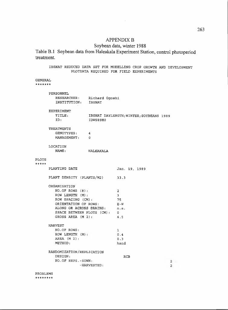
263
APPENDIX B Soybean data, winter 1988
Table B.l Soybean data from Haleakala Experiment Station, control photoperiod treatment.
IBSNAT REDUCED DATA SET FOR MODELLING CROP GROWTH AND DEVELOPMENT PLOTDATA REQUIRED FOR FIELD EXPERIMENTS
GENERAL* * * * * * *
PERSONNELRESEARCHER: INSTITUTION:
R ich a rd O gosh i IBSNAT
EXPERIMENT TITLE: ID :
IBSNAT DAYLENGTH/WINTER/SOYBEANS 1989 IDWS89H0
TREATMENTSGENOTYPES: 4MANAGEMENT: 0
LOCATIONNAME: HALEAKALA
PLOTS* * * * *
PLANTING DATE
PLANT DENSITY (PLANTS/M2)
Jan . 19 , 1989
33 .3
ORGANISATIONNO.OF ROWS ( # ) : 2ROW LENGTH (M ): 3ROW SPACING (CM ): 75ORIENTATION OF ROWS: E-WALONG OR ACROSS DRAINS: n .a .SPACE BETWEEN PLOTS (CM ): 0GROSS AREA ( M 2 ) : 4 .5
HARVESTNO.OF ROWS:ROW LENGTH (M) AREA ( M 2 ) : METHOD:
10 .40 .3hand
RANDOMIZATION/REPLICATIONDESIGN:NO.OF REPS.-SOWN:
-HARVESTED:
RCB
PROBLEMS* * * * * * * *
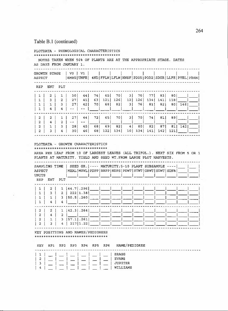
264
PLOTDATA - PHENOLOGICAL CHARACTERISTICS
Table B.l (continued)
NOTES TAKEN WHEN 50% OF PLANTS ARE AT THE APPROPRIATE STAGE. DATES AS DAYS FROM JANUARY 1 .
GROWTH STAGE | VO | VI | | | | | | | | | | |ASPECT |EMRG|UNFE| 4NDjFFLW|LFLWjNNSF1PDO5 jP0D2|SDGRjLLFEjPYEL1PBRNj
REP ENT PLT
30| 44| 74| 65| 7 0 1 3| 7 0 1 7 7 1 8 3 1 8 0 1______|27| 41| 63| 121| 126| 1 2 j 1 2 6 j 1 3 4 j 14l| 1 1 8 j______j'27| 42| 70| 68| 8 2 j 3| 7 6 j 8l| 8 2 | 80| 146|
-- I - I____I____I____I____I____I____I___I_____I____L
2413
1 I2 I3 I4 I
8927| 44| 72| 65l 7 0 |- I - I I I I.28| 45| 68| 69| 8 2 | 4| 8 0 | 8 2 | 87| 8l| 142|.30| 46| 68| 122| 1 3 4 j 1 0 j 1 3 4 j 1 4 l j 1 4 2 j 12l|
3| 70| 74| 81|J .
PLOTDATA - GROWTH CHARACTERISTICS
AREA PER LEAF FROM 10 OF LARGEST LEAVES (ALL T R IF O L .). NEXT SIX FROM 5 OR 1 PLANTS AT MATURITY. YIELD AND SEED WT.FROM LARGE PLOT HARVESTS.
SAMPLING TIME | SEED GR. | MATURITY; 5 -1 0 PLANT SUBSAMPLE |.ASPECT IMXAL|MXWL j PDPP|BRPP[NDPS|PDWT|STWT|GRWT|SDWT|SDN% ju n it s I I I I I I I I I I i;
REP ENT PLT
1 l44 .7| .296|2 I 2 2 2 l l .3 8 | '3 | 5 0 .5 | .2 6 0 | '4 I I L
. l _ l .J ____I.J ____I.
J I.
2413
1 |42.3| .264|2 I 1 L3 |57.1| .261|_4 I 217|l.22|^
.1____I.J ____!.
KEY POSITIONS AND NAMES/PEDIGREES
KEY RPl RP2 RP3 RP4 RP5 RP6 NAME/PEDIGREE
| l | _ l _ l _ l _ l _ l _ l BRAGG | 2 | _ | _ | _ 1 _ 1 _ | _ | EVANS | 3 | _ 1 _ | _ | _ | _ | _ | JUPITER | 4 | __ I I I I I I WILLIAMS
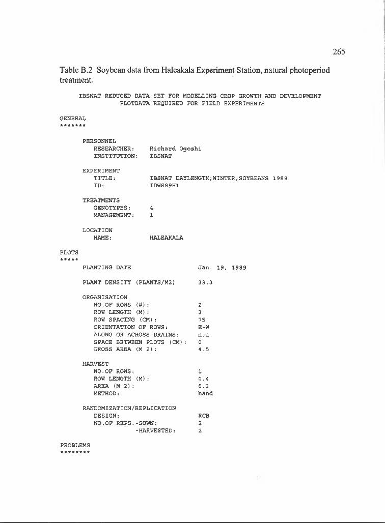
265
IBSNAT REDUCED DATA SET FOR MODELLING CROP GROWTH AND DEVELOPMENT PLOTDATA REQUIRED FOR FIELD EXPERIMENTS
GENERAL* * * * * * *
Table B.2 Soybean data from Haleakala Experiment Station, natural photoperiodtreatment.
PERSONNELRESEARCHER:INSTITUTION:
R ich a rd O gosh i IBSNAT
EXPERIMENT TITLE: ID :
IBSNAT DAYLENGTH;WINTER/SOYBEANS 1989 IDWS89H1
TREATMENTSGENOTYPES: 4MANAGEMENT: 1
LOCATIONNAME: HALEAKALA
PLOTS* * * * *
PLANTING DATE
PLANT DENSITY (PLANTS/M2)
Jan . 19 , 1989
3 3 .3
ORGANISATIONNO.OF ROWS ( # ) : 2ROW LENGTH (M ): 3ROW SPACING (CM ): 75ORIENTATION OF ROWS: E-WALONG OR ACROSS DRAINS: n .a .SPACE BETWEEN PLOTS (CM ): 0GROSS AREA ( M 2 ) : 4 .5
HARVESTNO.OF ROWS:ROW LENGTH (M ): AREA (M 2 ) : METHOD:
10 .40 .3hand
RANDOMIZATION/REPLICATIONDESIGN: RCBNO.OF REPS.-SOWN: 2
-HARVESTED: 2
PROBLEMS********
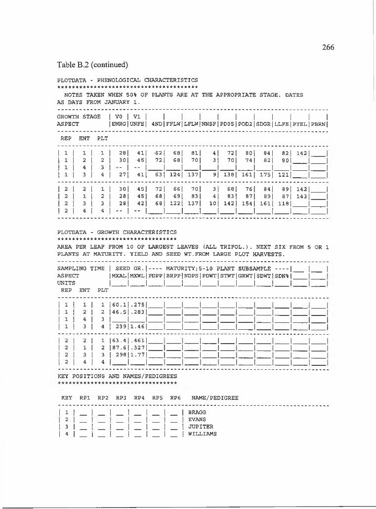
266
Table B.2 (continued)
PLOTDATA - PHENOLOGICAL CHARACTERISTICS ***************************************
NOTES TAKEN WHEN 50% OF PLANTS ARE AT THE APPROPRIATE STAGE. DATES AS DAYS FROM JANUARY 1 .
GROWTH STAGE ASPECT
I VO I VI I I I 1 I I I I I I I IEMRGIUNFE| 4ND|FFLW|LFLW|NNSF|PD05|P0D2|SDGR|LLFE|PYEL|PBRN|
REP ENT PLT
1234
28| 4l| •62{ 68| 8l| 4|3 o j 45] 72) 68| 7 0 j 3 |
- I - I I I I.
72 I 80 I70 I 74 I
J I.
84 I82 I
82 I 80]
142 I
I 27| 41] 63| 124| 137| 9j 138| 16l| 1 7 5 | 121]
1 I 30| 45| 72| 66| 7 0 | 3|2 I 28| 45| 68| 69| 8 3 j 4|3 I 28| 42| 68| 1 2 2 | 137| 1 0 j4 I - I - I____I____I____1____I.
68 I83 I
1421
76 I 87|
154 I
84 I 89|
161
89| 142| 87| 143|
118 1 IJ I.
PLOTDATA - GROWTH CHARACTERISTICS
AREA PER LEAF FROM 10 OF LARGEST LEAVES (ALL T R IF O L .). NEXT SIX FROM 5 OR 1 PLANTS AT MATURITY. YIELD AND SEED WT.FROM LARGE PLOT HARVESTS.
SAMPLING TIME | SEED GR. | MATURITY; 5 -1 0 PLANT SUBSAMPLE |_ASPECT IMXAL|MXWL j PDPP|BRPP|NDPS|PDWT|STWT|GRWT|SDWT|SDN% j 'u n it s I I I I I I I I I I i;
REP ENT PLT
1 | 60 .1| .275|2 |46.5| .283 j
3 I I I4 1 239|1.46|
J ____I.J ____I.
J .
J 1. J ___ IJ ___ I
1 | 63 .4| .461|2 | 8 7 .6 | .3 2 7 | ‘3 I 298|1.77|4 I I L
J ____I____I____ I.J ____I_I I.
.1 I I I.
KEY POSITIONS AND NAMES/PEDIGREES
KEY RPl RP2 RP3 RP4 RP5 RP6 NAME/PEDIGREE
| l | _ l _ l _ l _ l _ l _ l BRAGGEVANS
| 3 | __ 1 I I I I I JUPITER| 4 | _ 1 _ | _ | _ | _ | _ | WILLIAMS
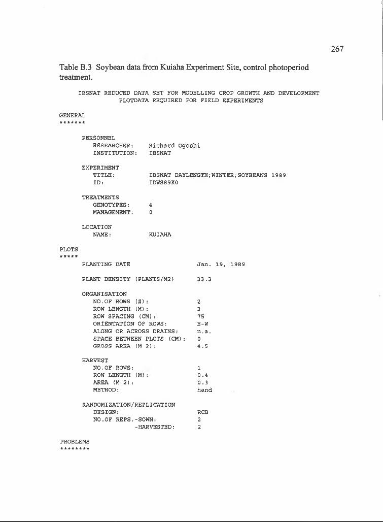
267
IBSNAT REDUCED DATA SET FOR MODELLING CROP GROWTH AND DEVELOPMENT PLOTDATA REQUIRED FOR FIELD EXPERIMENTS
GENERAL* * * * * * *
Table B.3 Soybean data from Kuiaha Experiment Site, control photoperiodtreatment.
PERSONNELRESEARCHER: INSTITUTION:
R ich a rd O gosh i IBSNAT
EXPERIMENT TITLE: ID :
IBSNAT DAYLENGTH/WINTER/SOYBEANS 1989 IDWS89K0
TREATMENTSGENOTYPES: 4MANAGEMENT: 0
LOCATIONNAME: KUIAHA
PLOTS* * * * *
PLANTING DATE
PLANT DENSITY ( PLANTS/M2)
Jan . 19 , 1989
3 3 .3
ORGANISATIONNO.OF ROWS ( # ) : 2ROW LENGTH (M ): 3ROW SPACING (CM ): 75ORIENTATION OF ROWS: E-WALONG OR ACROSS DRAINS: n .a .SPACE BETWEEN PLOTS (CM ): 0GROSS AREA ( M 2) : 4.5
HARVESTNO.OF ROWS: ROW LENGTH (M) AREA ( M 2 ) : METHOD:
10 .40 .3hand
RANDOMIZATION/REPLICATIONDESIGN: RCBNO.OF REPS.-SOWN: 2
-HARVESTED: 2
PROBLEMS* * * * * * * *
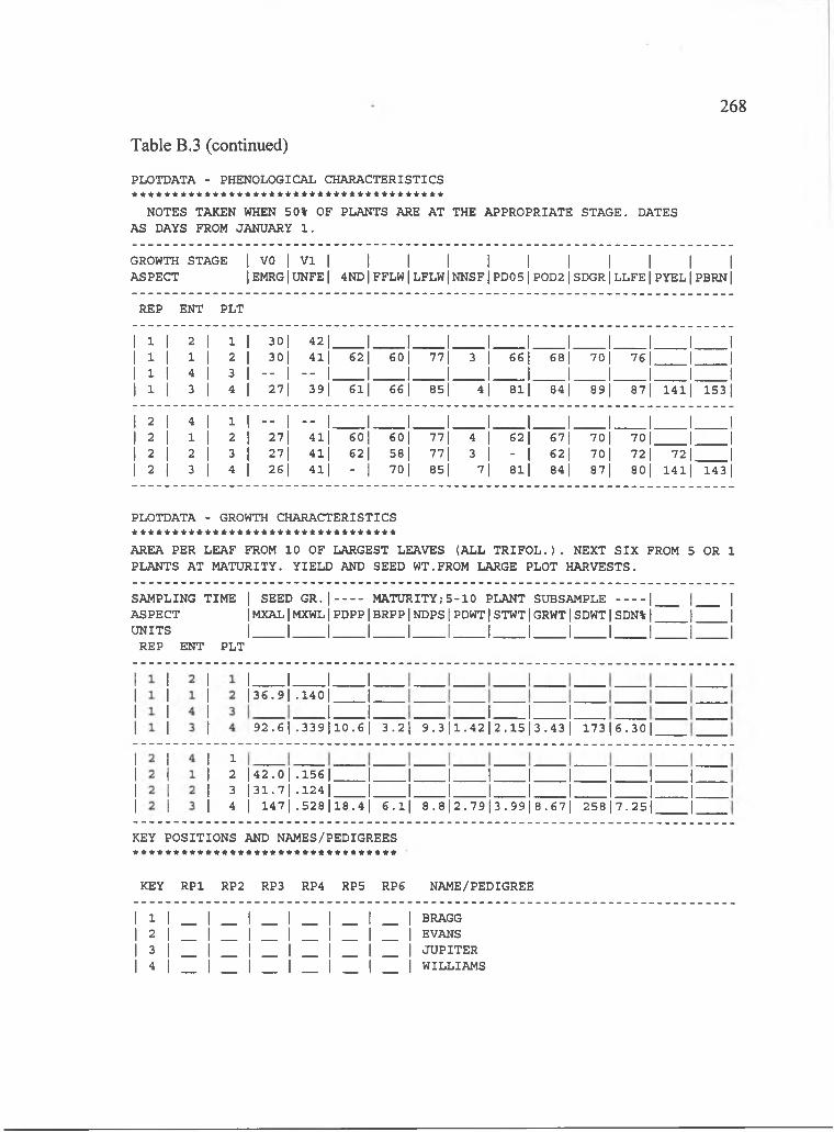
268
PLOTDATA - PHENOLOGICAL CHARACTERISTICS
Table B.3 (continued)
NOTES TAKEN WHEN 50% OF PLANTS ARE AT THE APPROPRIATE STAGE. DATES AS DAYS FROM JANUARY 1 .
GROWTH STAGE [ VO | V I | | | | | | | | | | |ASPECT lEMRGlUNFEl 4ND|FFLW|LFLW|NNSF|PDO5 jP0D 2jSDG RjLLFE|PYEL|PBR Nj
REP ENT PLT
1 3 1 2 1 1 1 30| 42| 1 1 1 1 1 1 1 1 1 11 1 1 1 1 2 1 30| 41| 62 1 60| 77| 3 1 66 1 68 1 70 1 76| 1 11 3 1 4 I 3 1 - 1 - 1 1 1 1 1 1 1 1 1 1 1I 1 I 3 1 4 1 27| 39| 611 66 1 85| 4| 81| 84 1 89| 87| 1411 1531
1 2 1 4 1 1 1 - - 1 - - 1 1 1 1 1 1 1 1 1 1 11 2 I 1 I 2 1 27| 41| 60 1 60| 77| 4 1 62 1 67 1 70| 70 1 1 1I 2 1 2 1 3 1 27| 41| 62 1 58 1 77| 3 1 - 1 62| 70| 72 1 72| 1I 2 I 3 1 4 1 26| 41| - 1 70 1 85| 7| 81| 84 1 87| 80| 141| 143|
PLOTDATA - GROWTH CHARACTERISTICS
AREA PER LEAF FROM 10 OF LARGEST LEAVES (ALL T R IF O L .). NEXT SIX FROM 5 OR 1 PLANTS AT MATURITY. YIELD AND SEED WT.FROM LARGE PLOT HARVESTS.
SAMPLING TIME | SEED G R .|------- MATURITY;5 -1 0 PLANT SUBSAMPLE -------- |ASPECT IMXAL|MXWL j PDPP|BRPP|NDPS|PDWT|STWT|GRWT|SDWT|SDN%|'u n it s I______I______I______I______I______I______I______I______I______I______i;
REP ENT PLT
I I I I.|36.9| .140| ______1.
.1____I. J I. J .| 9 2 .6 l .3 3 9 | 1 0 .6 | 3 .2 ] 9 . 3 |1 .4 2 |2 .1 5 |3 . 4 3 | 173|6.30|
I IJ ____I.1____I
1234
|42.0| .1 5 6 1 ______ I_____ I____ I_______I______I______I_____ I______I______I|31.7| .1 2 4 1 ______ I______I____ 1_______I______I______I_____ I______I______ 1_I 147| .528| 18 .4| 6 .l| 8 . 8 1 2 .7 9 |3 . 9 9 |8 . 6 7 | 2 5 8 | 7 .2 5 | ______|_
KEY POSITIONS AND NAMES/PEDIGREESit********************************KEY RPl RP2 RP3 RP4 RP5 RP6 NAME/PEDIGREE
| l | _ l _ l _ l _ l _ l _ l BRAGG | 2 | _ | _ | _ | _ 1 _ | _ | EVANS | 3 | _ | _ | _ | _ | _ | _ | JUPITER | 4 | __ I I I I I I WILLIAMS
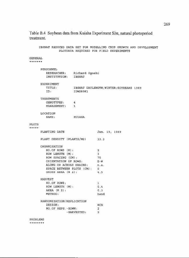
269
IBSNAT REDUCED DATA SET FOR MODELLING CROP GROWTH AND DEVELOPMENT PLOTDATA REQUIRED FOR FIELD EXPERIMENTS
GENERAL
Table B.4 Soybean data from Kuiaha Experiment Site, natural photoperiodtreatment.
PERSONNELRESEARCHER:INSTITUTION:
R ich a rd O gosh i IBSNAT
EXPERIMENT TITLE: ID :
IBSNAT DAYLENGTH;WINTER/SOYBEANS 1989 IDWS89K1
TREATMENTSGENOTYPES: 4MANAGEMENT: 1
LOCATIONNAME: KUIAHA
PLOTS* * * * *
PLANTING DATE
PLANT DENSITY (PLANTS/M2)
Jan . 19 , 1989
33 .3
ORGANISATIONNO.OF ROWS ( # ) : 2ROW LENGTH (M ): 3ROW SPACING (CM ): 75ORIENTATION OF ROWS: E-WALONG OR ACROSS DRAINS: n .a .SPACE BETWEEN PLOTS (CM): 0GROSS AREA ( M 2) : 4.5
HARVESTNO.OF ROWS: ROW LENGTH (M) AREA ( M 2 ) : METHOD:
10 .40 .3hand
RANDOMIZATION/REPLICATIONDESIGN: RCBNO.OF REPS.-SOWN: 2
-HARVESTED: 2
PROBLEMS
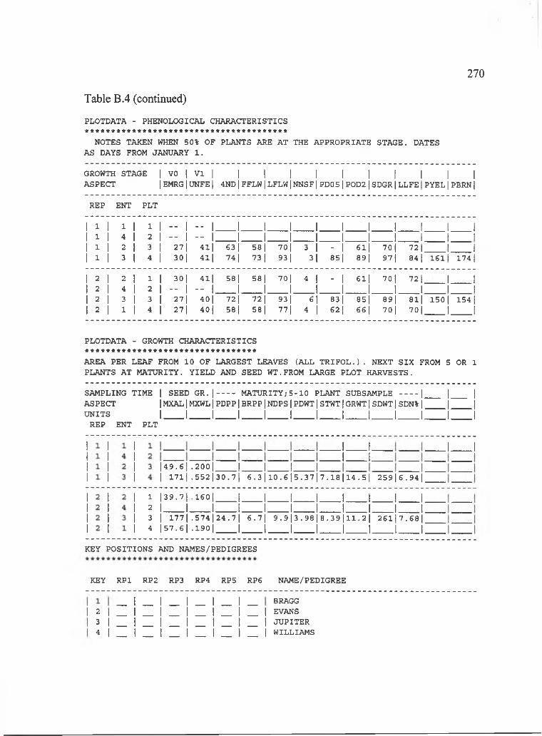
270
PLOTDATA - PHENOLOGICAL C3IARACTERISTICS
NOTES TAKEN WHEN 50% OF PLANTS ARE AT THE APPROPRIATE STAGE. DATES AS DAYS FROM JANUARY 1 .
Table B.4 (continued)
GROWTH STAGE | VO | VI | | | | | | | | | | |ASPECT |EMRG|UNFEl 4NDjFFLW jLFLW jNNSF|PD05jP0D2|SDGR|LLFEjPYEL|PBRNj
REP ENT PLT
1 3. 1 1 1 1 1 - 1 - 1 1 1 1 1 1 1 1 1 1 11 3. 1 4 1 2 1 - 1 - 1 1 1 1 1 1 1 1 1 1 11 3. 1 2 1 3 I 27| 41| 63 1 58 1 70 1 3 1 - 1 61| 70 1 721 1 11 3. 1 3 1 4 1 30| 41| 74 1 73 1 93 1 3| 85| 89| 97 1 84l 1 6 l l 1741
1 2 1 2 1 1 1 30| 41| 58| 58 1 70 1 4 1 - 1 61| 70 1 721 1 1I 2 I 4 1 2 1 - 1 - 1 1 1 1 1 1 1 1 1 1 11 2 1 3 I 3 1 27| 40| 72 1 72 1 93 1 6| 83 1 85| 89| 8 l l 1501 3B4l1 2 I 1 1 4 1 27| 40{ 58| 58| 77 1 4 1 62 1 66| 701 701 1 1
PLOTDATA - GROWTH CHARACTERISTICS * * * * * * * * * * * * * * * * * * * * * * * * * * * * * * * * *
AREA PER LEAF FROM 10 OF LARGEST LEAVES (ALL T R IF O L .). NEXT SIX FROM 5 OR 1 PLANTS AT MATURITY. YIELD AND SEED WT.FROM LARGE PLOT HARVESTS.
SAMPLING TIME | SEED GR. | MATURITY; 5 -1 0 PLANT SUBSAMPLE |___ |____ |ASPECT IMXAL|MXWL j PDPP|BRPP|NDPS|PDWT|STWT|GRWT|SDWT|SDN%|_____ | ______|u n it s I I I I I I I I I 1 I I I
REP ENT PLT
J ____I.J ____ I.
| 4 9 .6 | .2 0 0 | I I I I . __________________I 1 7 1 | .5 5 2 | 3 0 .7 l 6 .3 | 1 0 .6 | 5 .3 7 | 7 .1 8 | 1 4 .5 | 259|6.94|
J I
1 I 3 9 .7 t .1 6 0 l_____ I______I______I______I______ I______I_____ I______ I2 I I I I 1 I I I I I I.3 I 177| .5 7 4 |24.7| 6.7| 9 .9 | 3 . 9 8 |8 .3 9 |1 1 . 2 | 2 6 l| 7 .6 8 |4 | 5 7 .6 | .1 9 0 | _____ I______1______I______I______ I______I_____ 1______ i;
KEY POSITIONS AND NAMES/PEDIGREES
KEY RPl RP2 RP3 RP4 RP5 RP6
_ I _ I _ I _ I _ I _
NAME/PEDIGREE
BRAGG2 | _ l _ l _ l _ l _ l _ l EVANS3__I __ I I I 1 I I JUPITER4__I __ I I I 1 I I WILLIAMS
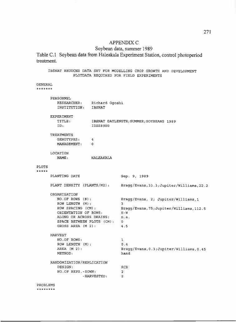
271
APPENDIX C Soybean data, summer 1989
Table C. 1 Soybean data from Haleakala Experiment Station, control photoperiod treatment.
IBSNAT REDUCED DATA SET FOR MODELLING CROP GROWTH AND DEVELOPMENT PLOTDATA REQUIRED FOR FIELD EXPERIMENTS
GENERAL
PERSONNELRESEARCHER:INSTITUTION:
R ich a rd O gosh i IBSNAT
EXPERIMENT TITLE: ID :
IBSNAT DAYLENGTH/SUMMER;SOYBEANS 1989 IDSS89H0
TREATMENTSGENOTYPES: 4MANAGEMENT: 0
LOCATIONNAME: HALEAKALA
PLOTS* * * * *
PLANTING DATE
PLANT DENSITY (PLANTS/M2):
ORGANISATIONNO.OF ROWS { # ) :ROW LENGTH (M ):ROW SPACING (CM ): ORIENTATION OF ROWS: ALONG OR ACROSS DRAINS: SPACE BETWEEN PLOTS (CM) GROSS AREA ( M 2 ) :
S ep . 9 , 1989
B r a g g /E v a n s ,3 3 .3 /J u p i t e r /W i l l i a m s ,2 2 .2
B ra gg /E v a n s , 2 ; J u p i t e r /W i l l i a m s , !3B r a g g /E v a n s ,7 5 ;J u p i t e r /W i l l i a m s ,1 1 2 .5E-Wn .a .0
4 .5
HARVESTNO.OF ROWS:ROW LENGTH (M ): AREA (M 2 ) : METHOD:
10 .4B r a g g /E v a n s ,0 . 3 /J u p i t e r /W i l l i a m s ,0 .4 5 hand
RANDOMIZATION/REPLICATIONDESIGN: RCBNO.OF REPS.-SOWN: 2
-HARVESTED: 2
PROBLEMS********
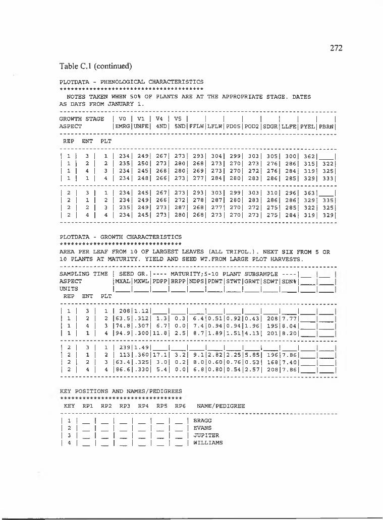
272
Table C.l (continued)
PLOTDATA - PHENOLOGICAL CHARACTERISTICS * * * * * * * * * * * * * * * * * * * * * * * * * * * * * * * * * * * * * * *
NOTES TAKEN WHEN 50% OF PLANTS ARE AT THE APPROPRIATE STAGE. DATES AS DAYS FROM JANUARY 1 .
GROWTH STAGE 1 VO 1 VI 1 V4 1 V5 1 1 1 1 1 1 1 1 1ASPECT 1EMRG1UNFE| 4ND| 5ND| FFLW| LFLW 1PD05|POD21SDGR1LLFE1PYEL| PBRNj
REP ENT PLT
1 1 1 3 1 1 1 234 1 249| 267| 273 1 293 1 304 1 299| 303 1 305| 300| 362| 11 1 1 2 1 2 1 235| 250| 273 1 280| 268| 273 1 270| 273 1 276 1 286| 315| 322|1 1 1 4 1 3 1 234 1 245 1 268 1 280| 269| 273 1 270| 272 1 276 1 284 1 319| 325|1 1 1 1 1 4 1 234 1 248 1 266 1 273 1 277| 284 1 280| 283 1 286| 285| 329| 333 1
1 2 1 3 1 1 1 234 1 245| 267| 273 1 293 1 303 1 299| 303 1 310 1 296| 363| 11 2 1 1 1 2 1 234 1 249| 266 1 272 1 278 1 287| 280| 283 1 286| 286| 329| 335|1 2 1 2 1 3 1 235| 249| 273 1 287| 268 1 277| 270 1 272 1 275| 285| 322 1 325|1 2 1 4 1 4 1 234 1 245| 273 1 280| 268| 273 1 270 1 273 1 275| 284 I 319| 329|
PLOTDATA - GROWTH CHARACTERISTICS * * * * * * * * * * * * * * * * * * * * * * * * * * * * * * * * *
AREA PER LEAF FROM 10 OF LARGEST LEAVES (ALL T R IF O L .). NEXT SIX FROM 5 OR 10 PLANTS AT MATURITY. YIELD AND SEED WT.FROM LARGE PLOT HARVESTS.
SAMPLING TIME | SEED G R .] ------- MATURITY;5 -1 0 PLANT SUBSAMPLE -------- \ASPECT 1MXAL|MXWL|PDPP|BRPP|NDPS|PDWT|STWT|GRWT|SDWT|SDN%|u n it s I______1______I______I______I______I______I______I______I______I______I
REP ENT PLT
1 1 3 1 1 1 208|1.12| 1 1 1 1 1 1 1 11 1 2 1 2 |63 .5| .312| 1.3| 0.3| 6 .4 l0 .5 l| 0 .9 2 | 0 .4 3 | 208|7.77|1 1 4 1 3 |74.8| .307| 6.7| 0.0| 7 .4 l0 .9 4 | 0 .9 4 | l .9 6 | 1 9 5 l8 .0 4 |1 1 1 1 4 |94.9| .3 0 0 | l l . 8 l 2.5| 8 .7 | 1 .8 9 | 1 .5 1 | 4 .1 3 1 201|8.20|
2 1 3 1 1 1 239|1.49| I 1 1 1 1 1 1 12 1 1 1 2 1 113| .360| 17 .1| 3.2| 9 .1 | 2 .8 2 | 2 .2 5 | 5 .8 5 | 1 9 6 l7 .8 6 |2 1 2 1 3 |63.4| .325| 3.0| 0.2| 8 .0 | 0 .6 0 | 0 .7 6 | 0 .5 3 | 168|7.40|2 1 4 1 4 |86 .6| .330| 5 . 4 l 0.0| 6 .8 | 0 .8 0 | 0 .5 4 | 2 .5 7 | 208|7.86|
KEY POSITIONS AND NAMES/PEDIGREES
KEY RPl RP2 RP3 RP4 RP5 RP6 NAME/PEDIGREE
| l | _ l _ l _ l _ l _ l _ l BRAGG | 2 | _ | _ | _ | _ 1 _ | _ | EVANS | 3 | _ | _ | _ | _ | _ | _ | JUPITER | 4 | _ | _ | _ | _ | _ 1 _ | WILLIAMS

273
IBSNAT REDUCED DATA SET FOR MODELLING CROP GROWTH AND DEVELOPMENT PLOTDATA REQUIRED FOR FIELD EXPERIMENTS
GENERAL
Table C.2 Soybean data from Haleakala Experiment Station, natural photoperiodtreatment.
PERSONNELRESEARCHER: INSTITUTION:
R ich a rd O gosh i IBSNAT
EXPERIMENT TITLE: ID :
IBSNAT DAYLENGTH/SUMMER/SOYBEANS 1989 IDSS89H1
TREATMENTSGENOTYPES: 4MANAGEMENT: 1
LOCATIONNAME: HALEAKALA
PLOTS* * * * *
PLANTING DATE
PLANT DENSITY (PLANTS/M2)
ORGANISATIONNO.OF ROWS (# ) :ROW LENGTH (M ):ROW SPACING (CM): ORIENTATION OF ROWS: ALONG OR ACROSS DRAINS: SPACE BETWEEN PLOTS (CM) GROSS AREA ( M 2 ) :
HARVESTNO.OF ROWS:ROW LENGTH (M ):AREA ( M 2 ) :METHOD:
RANDOMIZATION/REPLICATIONDESIGN:NO.OF REPS.-SOWN:
-HARVESTED:
S ep . 9 , 1989
B r a g g /E v a n s ,3 3 .3 /J u p i t e r /W i l l i a m s ,2 2 .2
B ra gg /E v a n s , 2 ; J u p i t e r /W i l l ia m s , 1 3B r a g g /E v a n s ,7 5 ;J u p i t e r /W i l l i a m s ,1 1 2 .5E-Wn .a .04 .5
10 .4B r a g g /E v a n s ,0 . 3 ; J u p i t e r /W i l l i a m s ,0 .4 5 hand
RCB22
PROBLEMSIt*******
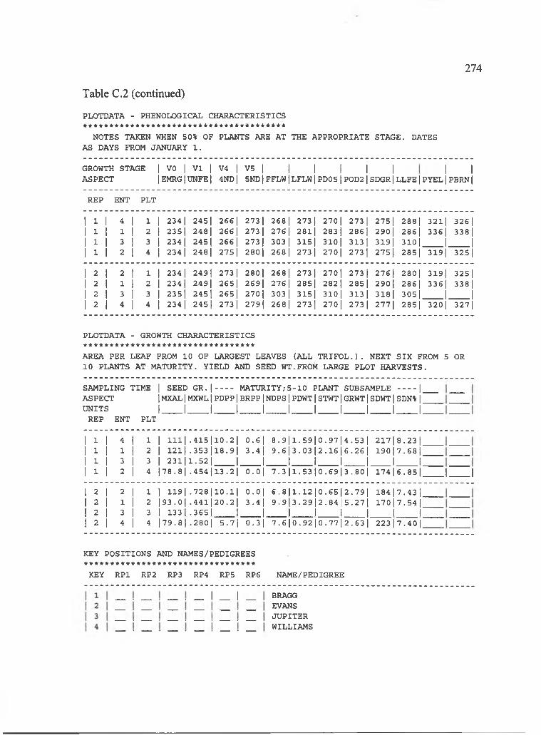
274
Table C.2 (continued)
PLOTDATA - PHENOLOGICAL CHARACTERISTICS * * * * * * * * * * * * * * * * * * * * * * * * * * * * * * * * * * * * * * *
NOTES TAKEN WHEN 50% OF PLANTS ARE AT THE APPROPRIATE STAGE. DATES AS DAYS FROM JANUARY 1 .
GROWTH STAGE 1 VO 1 VI 1 V4 1 V5 1 1 1 1 1 1 1 1ASPECT 1EMRG 1UNFE| 4ND| 5NDl FFLWl LFLWl PDOSl P0D21SDGR1LLFE1PYEL1PBRN1
REP ENT PLT
1 1 1 4 1 1 1 234 1 245| 2661 273 1 2681 273 1 270 1 273 1 2751 288 1 3211 32611 1 1 1 1 2 1t 2351 248| 266 I 273 1 276 I 2811 283 I 2861 290| 286 1 3361 338|1 1 1 3 I 3 1I 234 1 245 I 266 I 273 I 303 I 3151 310| 3131 319| 310 1 1 11 1 1 2 1 4 1! 234 1 248| 275 I 280 I 268 I 273 1 270| 273 1 2751 285| 3191 3251
1 2 1 2 1 1 11 234 1 249| 273 1 280 1 268 1 273 1 2701 273 1 2761 2801 3191 32511 2 1 1 I 2 11 234 1 249| 2651 269| 276 I 2851 282| 285| 290] 286| 336| 338 11 2 1 3 I 3 11 2351 2451 265| 270 I 303 I 315| 310| 3131 318| 305| 1 11 2 1 4 1 4 11 234 1 245 1 273 1 279| 268| 273 1 270 I 273 1 277 I 285| 3201 3271
PLOTDATA - GROWTH CHARACTERISTICS * * * * * * * * * * * * * * * * * * * * * * * * * * * * * * * * *
AREA PER LEAF FROM 10 OF LARGEST LEAVES (ALL T R IF O L .) . NEXT SIX FROM 5 OR 10 PLANTS AT MATURITY. YIELD AND SEED WT.FROM LARGE PLOT HARVESTS.
SAMPLING TIME | SEED GR. | MATURITY; 5 -1 0 PLANT SUBSAMPLE |ASPECT 1MXAL|MXWL j PDPP(BRPP|NDPS|PDWT|STWT|GRWT|SDWT|SDN%|u n i t s I I I I I I I I I I I
REP ENT PLT
1 1 4 1 1 1 m l . 4 1 5 1 1 0 . 2l 0 . 6 l 8 . 9 l 1 . 5 9 1 0 . 97 | | 4 . 5 3 l 2 1 7 | | 8 . 2 3 l1 I 1 1 2 I 1 2 1 1 . 3 5 3 1 1 8 . 9 | 3 . 4 1 9 . 61 | 3 . 0 3 | 2 . 1 6 | | 6 . 2 6 l 1 9 0 1| 7 . 6 8 l1 I 3 1 3 1 2 3 1 1 1 . 5 2 1 1 1 11 1 11 1 11 11 I 3 1 4 178 . 8 1 . 4 5 4 1 1 3 .21 o . o l 7 . 3 | | l . 5 3 l 0 . 6 9 | | 3 . 8 0 l 1 7 4 i| 6 . 8 5 l
3 1 3 1 1 1 1 1 9 1 . 7 2 8 | 1 0 . 1 1 O.Ol 6 . 8 | | 1 . 1 2 l 0 . 6 5 | | 2 . 7 9 l 1 8 4 j1 7 . 43 12 I 1 1 2 1 9 3 . o j . 4 4 1 | 2 0 . 2 | 3 . 4 1 9 .9 3 . 2 9 | 2 . 8 4 | 5 . 2 7 l 170 | 7 . 5 4 1 ,2 I 3 1 3 1 1 3 3 1 . 3 6 5 1 1 1 11 1 !1 1 1 13 1 4 1 4 l 7 9 . 8 1 . 2 8 0 1 5 . 7 l 0 . 3 1 7 . 6 | 1 0 . 9 2 1 0 . 7 7 ] | 2 . 6 3 l 2 2 3 1 7 . 4 0 l
J I
KEY POSITIONS AND NAMES/PEDIGREES * * * * * * * * * * * * * * * * * * * * * * * * * * * * * * * * *
KEY RPl RP2 RP3 RP4 RP5 RP6 NAME/PEDIGREE
I _ I BRAGGEVANSJUPITERWILLIAMS
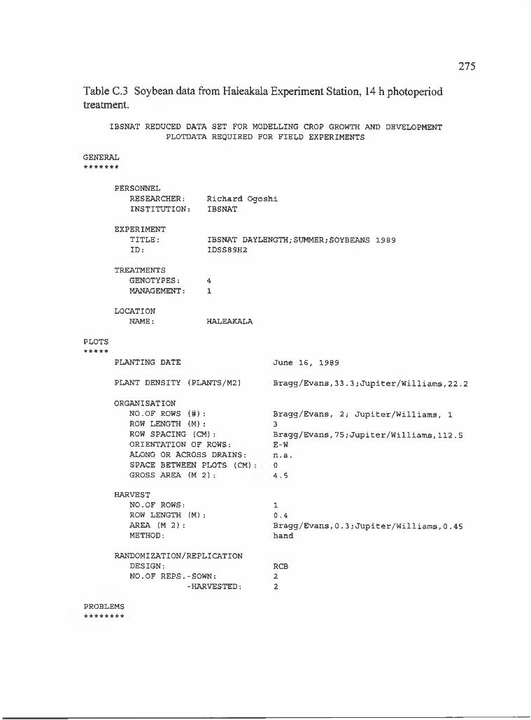
275
IBSNAT REDUCED DATA SET FOR MODELLING CROP GROWTH AND DEVELOPMENT PLOTDATA REQUIRED FOR FIELD EXPERIMENTS
GENERAL*******
Table C.3 Soybean data from Haleakala Experiment Station, 14 h photoperiodtreatment.
PERSONNELRESEARCHER:INSTITUTION:
R ich a rd O gosh i IBSNAT
EXPERIMENT TITLE: ID :
IBSNAT DAYLENGTH;SUMMER/SOYBEANS 1989 IDSS89H2
TREATMENTSGENOTYPES: 4MANAGEMENT: 1
LOCATIONNAME: HALEAKALA
PLOTS* * * * *
PLANTING DATE
PLANT DENSITY (PLANTS/M2)
ORGANISATIONNO.OF ROWS ( # ) :ROW LENGTH (M ):ROW SPACING (CM ): ORIENTATION OF ROWS: ALONG OR ACROSS DRAINS: SPACE BETWEEN PLOTS (CM) GROSS AREA ( M 2 ) :
June 16 , 1989
B r a g g /E v a n s ,3 3 . 3 ; J u p i t e r /W i l l ia m s , 2 2 .2
B ra gg /E v a n s , 2 ; J u p i t e r /W i l l ia m s , 1 3B r a g g /E v a n s ,7 5 ;J u p i t e r /W i l l i a m s ,1 1 2 .5E-Wn .a .04 .5
HARVESTNO.OF ROWS:ROW LENGTH (M ): AREA (M 2 ) : METHOD:
10 .4B r a g g /E v a n s ,0 . 3 ; J u p i t e r /W i l l i a m s ,0 .4 5 hand
RANDOMIZATION/REPLICATIONDESIGN: RCBNO.OF REPS.-SOWN: 2
-HARVESTED: 2
PROBLEMS
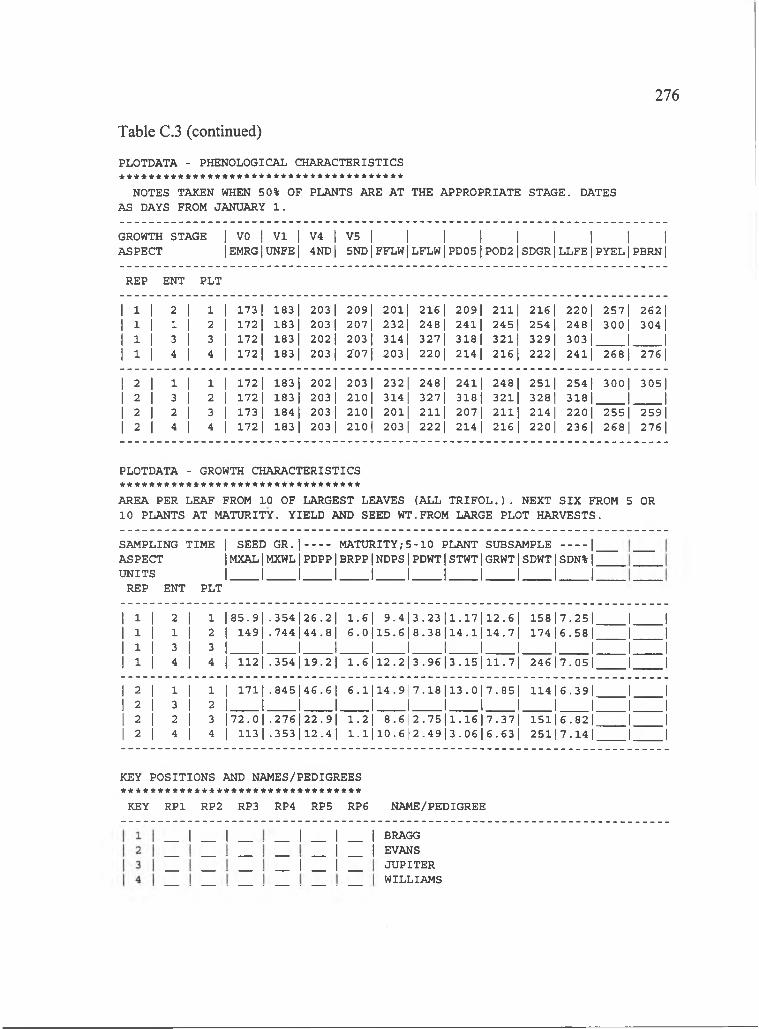
276
Table C.3 (continued)
PLOTDATA - PHENOLOGICAL CHARACTERISTICS * * * * * * * * * * * * * * * * * * * * * * * * * * * * * * * * * * * * * * *
NOTES TAKEN WHEN 50% OF PLANTS ARE AT THE APPROPRIATE STAGE. DATES AS DAYS FROM JANUARY 1 .
GROWTH STAGE 11 VO 1 VI 1 V4 1 V5 1 1 1 1 1 1 1 1 1ASPECT 1[EMRGj UNFEj 4ND| 5ND| FFLW| LFLW| PD05| P0D2| SDGR| LLFE| PYEL| PBRN|
REP ENT PLT
1 3 1 2 1 1 11 173 1 183 1 203 1 209| 201| 216| 209| 211| 216 1 220 1 257| 262|1 3. 1 1 1 2 11 172 1 183 1 203 1 207| 232| 248| 241| 245| 254 1 248 I 300 1 304 j1 3 1 3 j 3 11 172 1 183 I 202 1 203 1 314 I 327| 318 I 321| 329| 303| 1 11 1 1 4 1 4 !1 172 1 183 I 203 I 207 I 203 1 220 1 214 I 216 1 222 1 241| 268 1 276 1
1 2 1 1 1 1 1 172 1 183 1 202 1 203 1 232| 248 1 2411 248 1 251| 254 1 300 1 305 11 2 1 3 I 2 1 172 1 183 1 203 I 210| 314 1 327| 318| 321| 328 I 318| 1 11 2 1 2 I 3 1 173 1 184 I 203 I 210| 201| 211| 207| 211| 214 I 220| 255| 259|1 2 1 4 1 4 1 172 1 183 1 203 I 210| 203 I 222 1 214 I 216 1 220 I 236| 268 1 276 1
PLOTDATA - GROWTH CHARACTERISTICS * * * * * * * * * * * * * * * * * * * * * * * * * * * * * * * * *
AREA PER LEAF FROM 10 OF LARGEST LEAVES (ALL T R IF O L .). NEXT SIX FROM 5 OR 10 PLANTS AT MATURITY. YIELD AND SEED WT.FROM LARGE PLOT HARVESTS.
SAMPLING TIME | SEED GR. | MATURITY;5 -1 0 PLANT SUBSAMPLE |ASPECT IMXAL|MXWL|PDPP|BRPP|NDPS|PDWT|STWT|GRWT|SDWT|SDN% ju n it s I I I I I I I I I I I
REP ENT PLT
1 1 1 2 1 1 |85.9| .354| 26 .2| 1 .61 9-4|| 3 . 2 3 l l . l 7 l l 2 . 6 l 15817 .251 1 11 1 1 1 I 2 1 149| .744| 44 .8| 6 .0 l l5 .6 | | 8 .3 8 | l 4 . l | l 4 .7 l 17416 .581 1 11 1 1 3 1 3 1 1 1 1 1 11 1 1 1 1 1 1 11 1 1 4 1 4 ! 1 1 2 1.3 5 4 1 1 9 .2| 1 .6 112.2]| 3 . 9 6 l 3 .1 5 l l l . 7 l 2 4 617 .051 1 1
1 2 1 1 1 1 1 1711 .845| 46 .6| 6 .1 1 1 4 .9 | 7 .1 8 1 1 3 .0 1 7 .8 5 1 11416 .391 1 11 2 1 3 I 2 1, 1 1 1 ,1 ..... J 1 ... 1 1 1 1 1 1 11 2 1 2 1 3 |72.0| .276| 22 .9| 1 .2 l 8 .6 | 2 . 7 5 l l . l 6 l 7 . 3 7 l 1 5116 .821 1 11 3 I 4 1 4 1 113 1 .353| 12 .4| 1 .1 | 1 0 .6 | 2 .4 9 | 3 .0 6 | 6 .6 3 1 25117 .141 1 1
KEY POSITIONS AND NAMES/PEDIGREES * * * * * * * * * * * * * * * * * * * * * * * * * * * * * * * * *
KEY RPl RP2 RP3 RP4 RP5 RP6 NAME/PEDIGREE
I _ I I _ I
I _ II _ I
I BRAGG EVANS JUPITER WILLIAMS
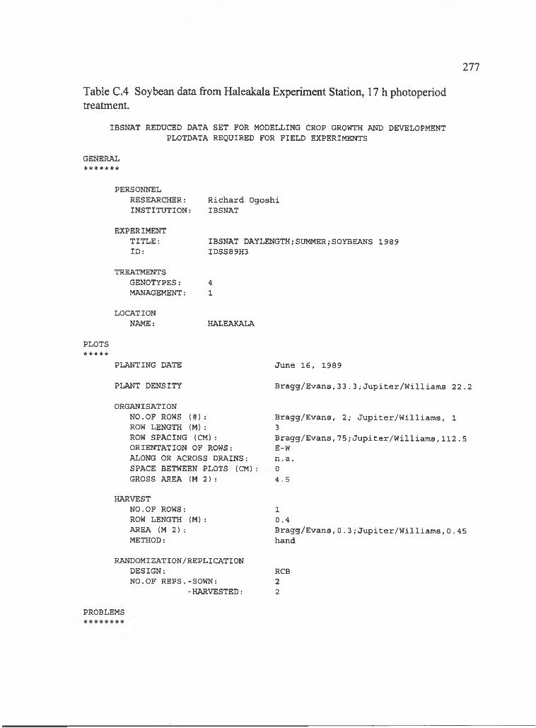
277
IBSNAT REDUCED DATA SET FOR MODELLING CROP GROWTH AND DEVELOPMENT PLOTDATA REQUIRED FOR FIELD EXPERIMENTS
GENERAL
Table C.4 Soybean data from Haleakala Experiment Station, 17 h photoperiodtreatment.
PERSONNELRESEARCHER: INSTITUTION:
R ich a rd O gosh i IBSNAT
EXPERIMENT TITLE: ID :
IBSNAT DAYLENGTH;SUMMER/SOYBEANS 1989 IDSS89H3
TREATMENTSGENOTYPES: 4MANAGEMENT: 1
LOCATIONNAME: HALEAKALA
PLOTS* * * * *
PLANTING DATE
PLANT DENSITY
ORGANISATIONNO.OF ROWS (#) :ROW LENGTH (M ):ROW SPACING (CM ): ORIENTATION OF ROWS: ALONG OR ACROSS DRAINS: SPACE BETWEEN PLOTS (CM) GROSS AREA ( M 2 ) :
June 16 , 1989
B r a g g /E v a n s ,3 3 .3 /J u p i t e r /W i l l i a m s 2 2 .2
B ra gg /E v a n s , 2 ; J u p i t e r /W i l l ia m s , 13B r a g g /E v a n s ,7 5 ;J u p i t e r /W i l l i a m s ,1 1 2 .5E-Wn .a .04 .5
HARVESTNO.OF ROWS:ROW LENGTH (M ):AREA (M 2 ) :METHOD:
RANDOMIZATION/REPLICATIONDESIGN:NO.OF REPS.-SOWN:
-HARVESTED:
10 .4B r a g g /E v a n s ,0 . 3 /J u p i t e r /W i l l i a m s ,0 .4 5 hand
RCB22
PROBLEMS
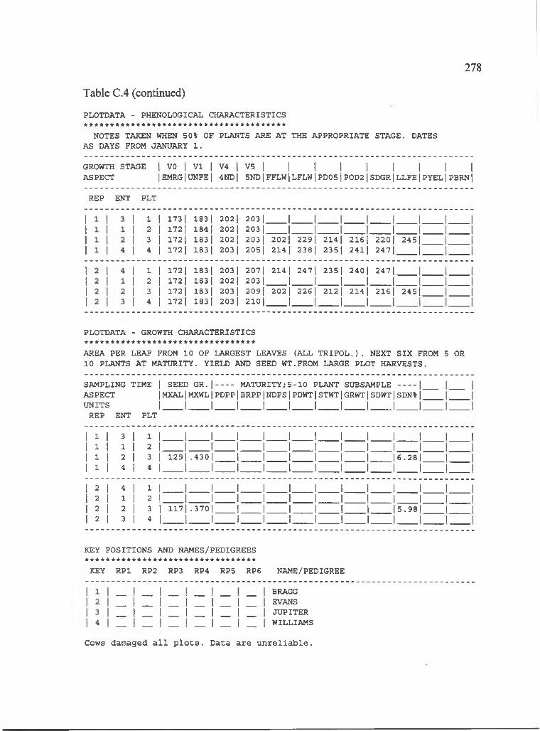
278
Table C.4 (continued)
PLOTDATA - PHENOLOGICAL CHARACTERISTICS
NOTES TAKEN WHEN 50% OF PLANTS ARE AT THE APPROPRIATE STAGE. DATES AS DAYS FROM JANUARY 1 .
GROWTH STAGE j VO | VI | V4 | V5 | | \ \ \ \ \ \ |ASPECT |EMRG|UNFE| 4ND| 5NDjFFLW|LFLW|PDO5 jP0D2jSDGRjLLFEjPYELjPBRNj
REP ENT PLT
1 I 173| 183| 2021 2031______1.2 1 172| 184] 202| 203 j______j_____ 1 .L3 1 1721 1831 2021 2031 2021 2291 2141 2161 2201 24514 I 172| 183| 203| 205| 2 1 4 j 2381 235| 24l| 247|______j
1 1 1721 1831 2031 2071 2141 2471 2351 240l 24712 1 1721 1831 2021 203 1____ 1______1______1______1_____ L3 1 1721 1831 2031 2091 2021 2261 2121 2141 2161 245l_4___ I 172| 183| 203| 210|____ j______j______j______j______| _____
PLOTDATA - GROWTH CHARACTERISTICS * * * * * * * * * * * * * * * * * * * * * * * * * * * * * * * * *AREA PER LEAF FROM 10 OF LARGEST LEAVES (ALL T R IF O L .). NEXT SIX FROM 5 10 PLANTS AT MATURITY. YIELD AND SEED WT.FROM LARGE PLOT HARVESTS.
OR
SAMPLING TIME 1 SEED GR. | MATURITY;5 -1 0 PLANT SUBSAMPLE 1ASPECT IMXAL1MXWL j PDPP1BRPP1NDPS1PDWT1STWT1GRWT1SDWT1SDN% jUNITS 1_____ 1______I______1______1______1______1______1______1______1______ 1
REP ENT PLT
1 1 1 3 1 1 1 1 1 1 1 1 1 1 1 1 1 1 1
1 1 1 1 1 2 1 1 1 1 1 1 1 1 1 1 1 1 1
1 1 1 2 3 1 1 2 9 1 . 4 3 0 1 1 1 1 1 1 1 1 6 . 2 8 1 1 1
1 1 1 4 1 4 1 1 1 1 1 1 1 1 1 1 1 1 1
1 2 1 4 1 1 1 J 1 1 1 1 1 1 1 1 1 1 1
1 2 1 1 1 2 1 J 1 1 1 1 1 1 1 1 1 1 I
1 2 1 2 1 3 11 1 1 7 1 . 3 7 0 1 1 1 1 1 1 1 1 5 . 9 8 1 1 1
1 2 1 3 1 4 1I 1 1 1 1 1 1 1 1 1 1 1 1
KEY POSITIONS AND NAMES/PEDIGREES * * * * * * * * * * * * * * * * * * * * * * * * * * * * * * * * *
KEY RPl RP2 RP3 RP4 RP5 RP6 NAME/PEDIGREE
I_ I _ I _ I _ I _ I __ I _ I _ I _ I _ I _
I _ 1
BRAGGEVANSJUPITERWILLIAMS
Cows damaged a l l p l o t s . Data a re u n r e l i a b l e .
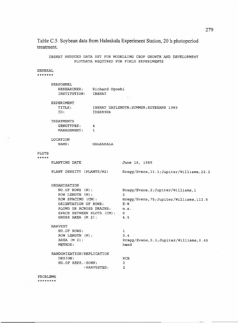
279
IBSNAT REDUCED DATA SET FOR MODELLING CROP GROWTH AND DEVELOPMENT PLOTDATA REQUIRED FOR FIELD EXPERIMENTS
GENERAL
Table C.5 Soybean data from Haleakala Experiment Station, 20 h photoperiodtreatment.
PERSONNELRESEARCHER:INSTITUTION:
R ich a rd O gosh i IBSNAT
EXPERIMENTTITLE:ID :
IBSNAT DAYLENGTH;SUMMER/SOYBEANS 1989 IDSS89H4
TREATMENTSGENOTYPES: 4MANAGEMENT: 1
LOCATIONNAME: HALEAKALA
PLOTS*****
PLANTING DATE
PLANT DENSITY (PLANTS/M2)
June 16 , 1989
B r a g g /E v a n s ,3 3 .3 /J u p i t e r /W i l l i a m s ,2 2 .2
ORGANISATIONNO.OF ROWS ( # ) :ROW LENGTH (M ):ROW SPACING (CM ): ORIENTATION OF ROWS: ALONG OR ACROSS DRAINS: SPACE BETWEEN PLOTS (CM) GROSS AREA ( M 2 ) :
B r a g g /E v a n s ,2 /J u p i t e r /W i l l i a m s ,1 3B r a g g /E v a n s ,7 5 ;J u p i t e r /W i l l i a m s ,1 1 2 .5E-Wn .a .04 .5
HARVESTNO.OF ROWS:ROW LENGTH (M ): AREA ( M 2 ) : METHOD:
10 .4B r a g g /E v a n s ,0 . 3 /J u p i t e r /W i l l i a m s ,0 .4 5 hand
RANDOMIZATION/REPLICATIONDESIGN: RCBNO.OF REPS.-SOWN: 2
-HARVESTED: 2
PROBLEMS
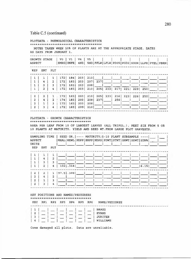
280
Table C.5 (continued)
PLOTDATA - PHENOLOGICAL CHARACTERISTICS * * * * * * * * * * * * * * * * * * * * * * * * * * * * * * * * * * * * * * *
NOTES TAKEN WHEN 50% OF PLANTS ARE AT THE APPROPRIATE STAGE. DATES AS DAYS FROM JANUARY 1 .
GROWTH STAGE | VO | V I | V4 | V5 | ] ] | | \ | | [ASPECT |EMRG|UNFE| 4ND| 5ND|FFLWjLFLWjPDO5 jP0D2jSDGRjLLFEjPYELjPBRNj
REP ENT PLT
1 1 1 1 1 1 11 1721 184 1 203 1 210 1 1 1 1 1 1 1 1 11 3. 1 4 1 2 11 1721 183 I 203 1 207| 2371 1 1 ..................................................1 3. 1 3 I 3 11 172 1 183 I 203 1 208 I 1 1 1 1 1 1 1 11 3. 1 2 1 4 11 172 1 183 I 203 I 210 I 2051 233 1 2171 2 2 l l 229| 250| | |
1 2 1 2 1 1 1 172 1 183 1 203 1 2101 2051 233 1 216 1 2231 2261 2501 | |1 2 1 4 I 2 1 174 1 183 1 203 I 208| 2371 1 250 I 1 1 1 1 11 2 1 1 1 3 1 172 1 183 I 203 I 208 1 1 1 1 1 1 1 1 11 2 1 3 I 4 1 172 1 183 1 209| 210| 1 1 1 1 1 1 1 1
PLOTDATA - GROWTH CHARACTERISTICS
AREA PER LEAF FROM 10 OF LARGEST LEAVES (ALL T R IF O L .). NEXT SIX FROM 5 OR 10 PLANTS AT MATURITY. YIELD AND SEED WT.FROM LARGE PLOT HARVESTS.
SAMPLING TIME | SEED GR. | MATURITY; 5 -1 0 PLANT SUBSAMPLE |ASPECT IMXAL|MXWL j PDPP|BRPP|NDPS|PDWT|STWT|GRWT|SDWT|SDN% ju n it s I I I I I I I 1 I I i;
REP ENT PLT
I__ IJ ___ IJ ___ I
J I.
I I____I.1 0 2 | . 3 1 4 1 ______I.
J .
6 .1 5
1 | 9 7 .5 l .30812 I_I I3 I_I I4 I I I
KEY POSITIONS AND NAMES/PEDIGREES * * * * * * * * * * * * * * * * * * * * * * * * * * * * * * * * *
KEY RPl RP2 RP3 RP4 RP5 RP6 NAME/PEDIGREE
I
_ I _ I _ I _
Cows damaged a l l p l o t s .
BRAGGEVANSJUPITERWILLIAMS
Data a re u n r e l i a b l e .
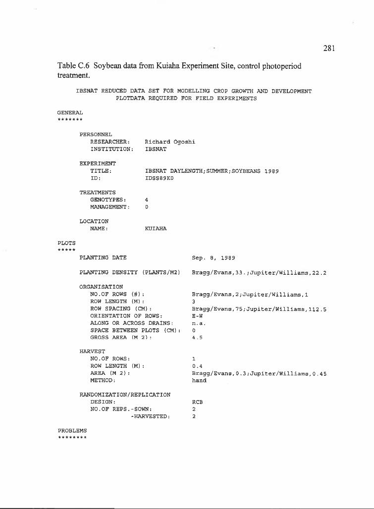
281
IBSNAT REDUCED DATA SET FOR MODELLING CROP GROWTH AND DEVELOPMENT PLOTDATA REQUIRED FOR FIELD EXPERIMENTS
GENERAL
Table C.6 Soybean data from Kuiaha Experiment Site, control photoperiodtreatment.
PERSONNELRESEARCHER:INSTITUTION:
R ich a rd O gosh i IBSNAT
EXPERIMENT TITLE: ID :
IBSNAT DAYLENGTH/SUMMER/SOYBEANS 1989 IDSS89K0
TREATMENTSGENOTYPES: 4MANAGEMENT: 0
LOCATIONNAME: KUIAHA
PLOTS* * * * *
PLANTING DATE
PLANTING DENSITY (PLANTS/M2)
ORGANISATIONNO.OF ROWS ( # ) :ROW LENGTH (M ):ROW SPACING (CM ): ORIENTATION OF ROWS: ALONG OR ACROSS DRAINS: SPACE BETWEEN PLOTS (CM ): GROSS AREA ( M 2 ) :
S ep . 8 , 1989
B r a g g /E v a n s ,3 3 . ; J u p i t e r /W i l l i a m s ,2 2 .2
B ra g g /E v a n s , 2 ; J u p i t e r /W i l l i a m s ,1 3B r a g g /E v a n s ,7 5 ;J u p i t e r /W i l l i a m s ,1 1 2 .5E-Wn . a .04 . 5
HARVESTNO.OF ROWS:ROW LENGTH (M ):AREA ( M 2 ) :METHOD:
RANDOMIZATION/REPLICATIONDESIGN:NO.OF REPS.-SOWN:
-HARVESTED:
10 .4B r a g g /E v a n s ,0 . 3 ; J u p i t e r /W i l l i a m s ,0 .4 5 hand
RCB22
PROBLEMS********

282
Table C.6 (continued)
PLOTDATA - PHENOLOGICAL CHARACTERISTICS * * * * * * * * * * * * * * * * * * * * * * * * * * * * * * * * * * * * * * *NOTES TAKEN WHEN 50% OF PLANTS ARE AT THE APPROPRIATE STAGE. DATES AS DAYS FROM JANUARY 1 .
GROWTH STAGE 1 VO 1 VI 1 V4 1 V5 1 1 1 1 1 1 1 1 1ASPECT 1EMRG1UNFE] 4ND| 5ND| FFLW| LFLW| PD05| P0D2j SDGR| LLFE1:PYEL| PBRNj
REP ENT PLT
1 1 1 3 1 1 1 256 1 265 1 284 1 293 1 296 1 307| 304 1 307| 311| 307| 356| 362|1 1 1 1 1 2 1 256 1 266 1 281| 292 I 284 I 293 1 289| 291| 294 1 296 1 337| 340|1 1 1 2 1 3 1 257 1 265| 286| - 1 279| 290 1 282| 285| 289| 286] 326] 332|1 1 1 4 1 4 1 256 1 265| 286| - 1 28l| 294 1 284 I 287| 289| 293 I 3331 338|
1 2 1 2 1 1 1 256 1 265| 286| - 1 278 1 290| 282 1 286 1 291| 291| 326| 33211 2 1 3 1 2 1 256 1 264 I 280| 285| 294 1 307| 303 I 305| 310| 306| 356| 362|1 2 1 1 I 3 11 2561 265 1 280| 285| 2811 290{ 288| 291| 292| 292| 338| 342 I1 2 1 4 1 4 1 256 1 264 j 280| 286{ 278 1 290 I 283 I 287| 291| 303| 335| 338|
PLOTDATA - GROWTH CHARACTERISTICS *********************************AREA PER LEAF FROM 10 OF LARGEST LEAVES (ALL T R IF O L .). NEXT SIX FROM 5 OR 10 PLANTS AT MATURITY. YIELD AND SEED WT.FROM LARGE PLOT HARVESTS.
SAMPLING TIME | SEED G R .|------- MATURITY;5 -1 0 PLANT SUBSAMPLE -------- |ASPECT IMXAL|MXWL j PDPP|BRPP|NDPS|PDWT|STWT|GRWT|SDWT|SDN% ju n it s I______I______I______I______I______I______I______t______I______I______I
REP ENT PLT
1 1 1 3 1 1 1 115| .376| 10 .3| 1 .91 9.8|11.55 | 1 .33|3.33| 188 1|6.67|1 1 1 1 I 2 | 8 5 .9 | .3 5 2 | 1 0 .6 | 2 .41 8.5|11.61 | l.3 5 | 4 .4 6 | 209||7.10|1 1 1 2 I 3 |49 .2| .139| 9.6| 0.5| 6.2| 1 .1 9 | 0 .50|3.43| 164 116.82|1 1 1 4 1 4 1 - 1 - 1 7.0| 0.3| 6.4| 1 .0 8 | 0 .35|3.19| 199 17.001
1 2 1 2 1 1 |45 .9| .141| 6.9| 0.0| 5 .5 !10.76 |0.66| 2 .33| 1671|6.61|1 3 1 3 I 2 1 179| .986| 23 .7| 4.3| 1 1 .5 ! 3 .67 | 3 .3 3 | 6 .8 l| 205 | 7.49(1 3 1 1 1 3 I 105| .523 I15.7| 2.3| 8.2| 2 .6 7 l2 .0 9 | 7 .7 2 | 234 | 7 .52 lI 2 1 4 1 4 |74.9| .206| 19 .5| 1.0| 1 0 .6 | 3 .3 9 | 1 .7 7 | 9 .3 5 | 189 16.331
KEY POSITIONS AND NAMES/PEDIGREES * * * * * * * * * * * * * * * * * * * * * * * * * * * * * * * * *
KEY RPl RP2 RP3 RP4 RP5 RP6 NAME/PEDIGREE
| l | _ l _ l _ l _ l _ l _ l BRAGG | 2 | _ | _ | _ | _ | _ 1 _ | EVANS I 3 l _ | _ | _ | _ | _ | _ l JUPITER | 4 | __ I 1 1 I I___ I WILLIAMS
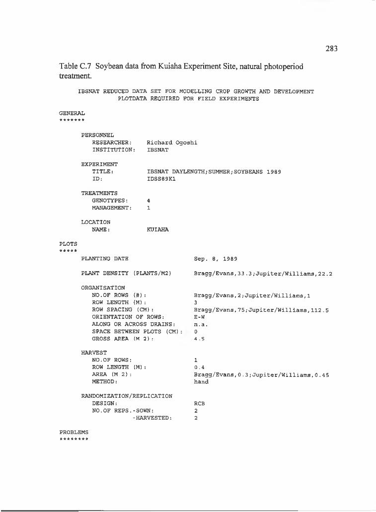
283
IBSNAT REDUCED DATA SET FOR MODELLING CROP GROWTH AND DEVELOPMENT PLOTDATA REQUIRED FOR FIELD EXPERIMENTS
GENERAL
Table C.l Soybean data from Kuiaha Experiment Site, natural photoperiodtreatment.
PERSONNELRESEARCHER:INSTITUTION:
R ich a rd O gosh i IBSNAT
EXPERIMENT TITLE: ID :
IBSNAT DAYLENGTH;SUMMER/SOYBEANS 1989 IDSS89K1
TREATMENTSGENOTYPES: 4MANAGEMENT: 1
LOCATIONNAME: KUIAHA
PLOTS* * * * *
PLANTING DATE
PLANT DENSITY (PLANTS/M2)
ORGANISATIONNO.OF ROWS { # ) :ROW LENGTH (M ):ROW SPACING (CM): ORIENTATION OF ROWS: ALONG OR ACROSS DRAINS: SPACE BETWEEN PLOTS (CM) GROSS AREA ( M 2 ) :
S ep . 8 , 1989
B r a g g /E v a n s ,3 3 . 3 ; J u p i t e r /W i l l i a m s ,2 2 .2
B r a g g /E v a n s ,2 ; J u p i t e r /W i l l i a m s ,1 3B r a g g /E v a n s ,7 5 ;J u p i t e r /W i l l i a m s ,1 1 2 .5E-Wn .a .04.5
HARVESTNO.OF ROWS:ROW LENGTH (M ):AREA ( M 2 ) :METHOD:
RANDOMIZATION/REPLICATIONDESIGN:NO.OF REPS.-SOWN:
-HARVESTED:
10 .4B r a g g /E v a n s ,0 . 3 ; J u p i t e r /W i l l i a m s ,0 .4 5 hand
RCB22
PROBLEMS*««■****■*
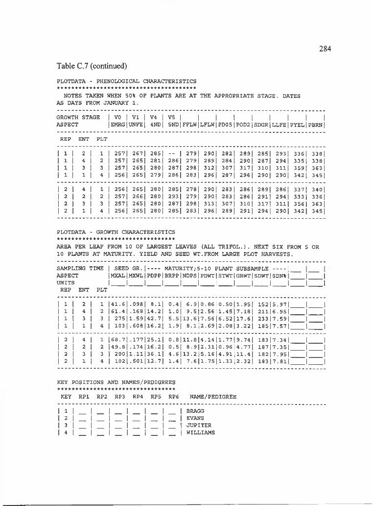
284
Table C.7 (continued)
PLOTDATA - PHENOLOGICAL CHARACTERISTICS * * * * * * * * * * * * * * * * * * * * * * * * * * * * * * * * * * * * * * *
NOTES TAKEN WHEN 50% OF PLANTS ARE AT THE APPROPRIATE STAGE. DATES AS DAYS FROM JANUARY 1 .
GROWTH STAGE 1 VO 1 V3 1 V4 1 V5 1 1 1 1 1 1 1 1 1ASPECT 1EMRGj UNFE| 4ND| 5ND| FFLW| LFLW| PD05| P0D21SDGR1LLFE|PYEL|PBRN|
REP ENT PLT
1 3 1 3 1 3 1 257| 267| 285| - 1 279| 290 1 282| 289 1 385| 293| 336| 338 11 3 I 4 1 3 1 257| 265| 281| 286 1 279| 289| 284 I 290 1 287| 294 I 3351 338|1 3 1 3 1 3 1 257 1 265| 280| 287| 298| 312 1 307| 317 1 310| 331| 3591 363 11 3 I 1 I 4 1 256 1 265| 279| 286 I 283 I 296 1 287| 296 1 290| 290| 3421 345|
1 3 1 4 1 3 1 256 1 265| 280| 285| 278 1 290{ 283 1 286 1 289| 286| 3371 340 11 3 1 2 I 2 11 3571 266| 280| 293 1 279| 290| 283 1 286 1 391| 294 3331 336|1 3 1 3 1 3 11 3571 265| 280| 287| 298| 3331 307| 310 1 317| 331| 356 1 363 I1 3 1 1 I 4 1 356 1 265| 280| 285| 283 I 296 1 289| 291 1 394 1 290| 342| 345|
PLOTDATA - GROWTH CHARACTERISTICS * * * * * * * * * * * * * * * * * * * * * * * * * * * * * * * * *AREA PER LEAF FROM 10 OF LARGEST LEAVES (ALL T R IF O L .). NEXT SIX FROM 5 OR 10 PLANTS AT MATURITY. YIELD AND SEED WT.FROM LARGE PLOT HARVESTS.
SAMPLING TIME | SEED GR. | MATURITY; 5 -1 0 PLANT SUBSAMPLE IASPECT 1MXAL1MXWL11PDPP1BRPP1NDPS1PDWT|STWT|GRWT1SDWT|SDN%| | |UNITS 1 1 11 1 .,1, 1 1 11 1 1 1 1 1
REP ENT PLT
1 3 1 3 1 1 l4 1 .6 l .0 9 8 | 1 8-31 0 .4 l 6.9||0.86 10.50|| 3 .95 l 1 5 2 | 5 .9 7 l 1 11 3 1 4 1 2 | 6 1 .4 | .168 |34.2l l . o j 9.5|[2.56| 3.45|| 7 .18 l 31116 .951 1 11 3 1 3 I 3 1 2 7 5 l l .5 9 l 4 2 .7 l 5 .5 | 1 3 .6 | |7.56|16.52|| 37 .6 l 3 3 3 | 7 .5 9 l 1 11 3 1 1 I 4 1 1 0 3 1 .6 0 8 j136.21 1.9| 8 .1 |3.69|12.08 !13.221 1 8 5 | 7 .5 7 l 1 1
1 3 1 4 1 1 1 6 8 .7 1 .1 7 7 1 2 5 . l l 0 . 8 l l l . 8 l 4 . 1 4 | I3 .7 7 j| 9 .74 l 1 8 3 | 7 .3 4 l 1 11 3 1 3 1 2 l 4 9 . 8 l .174 |16.21 0 .5 l 8.9||3.31|10.96 | 4 .77 l 18717 .351 1 11 3 1 3 I 3 I 2 0 0 l l . l l | 3 6 .l l 4 .6 | 1 3 .2 |5.16|14.91 131.41 18217 .951 1 11 3 1 1 I 4 1 1 0 2 1 .5 0 1 1 1 2 .7l 1 .41 7.6||3.75||3.33 12.321 18317 .811 1 1
KEY POSITIONS AND NAMES/PEDIGREES
KEY RPl RP2 RP3 RP4 RP5 RP6 NAME/PEDIGREE
| l | _ l _ l _ l _ l _ l _ l BRAGG | 2 | _ | _ | _ | _ | _ | _ | EVANS | 3 | _ | _ | _ | _ | _ | _ | JUPITER | 4 | __ I I I 1 I 1 WILLIAMS
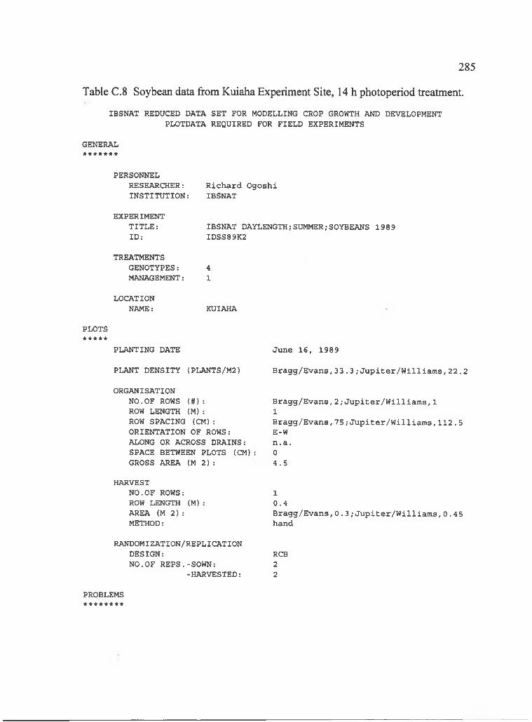
285
IBSNAT REDUCED DATA SET FOR MODELLING CROP GROWTH AND DEVELOPMENT PLOTDATA REQUIRED FOR FIELD EXPERIMENTS
Table C.8 Soybean data from Kuiaha Experiment Site, 14 h photoperiod treatment.
GENERAL
PERSONNELRESEARCHER: INSTITUTION:
R ich a rd O gosh i IBSNAT
EXPERIMENT TITLE: ID :
IBSNAT DAYLENGTH/SUMMER/SOYBEANS 1989 IDSS89K2
TREATMENTSGENOTYPES: 4MANAGEMENT: 1
LOCATIONNAME: KUIAHA
PLOTS* * * * *
PLANTING DATE
PLANT DENSITY (PLANTS/M2)
ORGANISATIONNO.OF ROWS ( # ) :ROW LENGTH (M ):ROW SPACING (CM): ORIENTATION OF ROWS: ALONG OR ACROSS DRAINS: SPACE BETWEEN PLOTS (CM) GROSS AREA ( M 2 ) :
HARVESTNO.OF ROWS:ROW LENGTH (M ):AREA ( M 2 ) :METHOD:
June 16 , 1989
B r a g g /E v a n s ,3 3 .3 /J u p i t e r /W i l l i a m s ,2 2 .2
B r a g g /E v a n s ,2 /J u p i t e r /W i l l i a m s ,1 1B r a g g /E v a n s ,7 5 ;J u p i t e r /W i l l i a m s ,1 1 2 .5E-Wn .a .0
4 .5
10 .4B r a g g /E v a n s ,0 . 3 /J u p i t e r /W i l l i a m s ,0 .4 5 hand
RANDOMIZATION/REPLICATIONDESIGN: RCBNO.OF REPS.-SOWN: 2
-HARVESTED: 2
PROBLEMS********
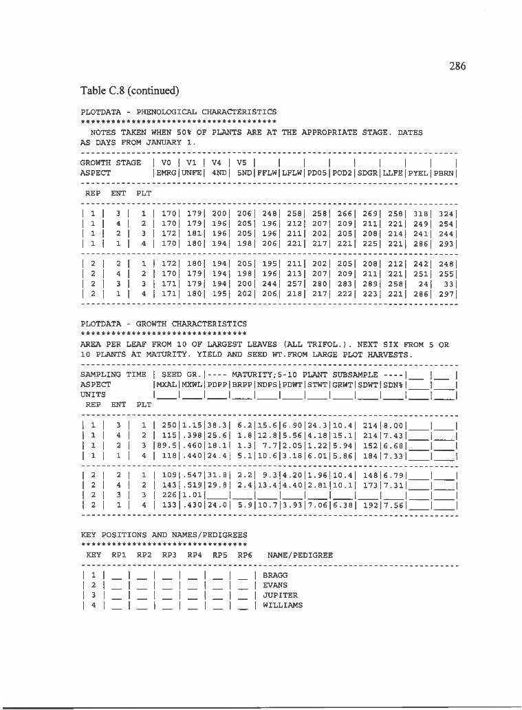
286
Table C.8 (continued)
PLOTDATA - PHENOLOGICAL CHARACTERISTICS * * * * * * * * * * * * * * * * * * * * * * * * * * * * * * * * * * * * * * *
NOTES TAKEN WHEN 50% OF PLANTS ARE AT THE APPROPRIATE STAGE. DATES AS DAYS FROM JANUARY 1 .
GROWTH STAGE 1 VO 1 VI 1 V4 1 V5 1 1 1 1 1 1 1 1 1ASPECT 1EMRG1UNFE| 4ND| 5ND1FFLW1LFLW1PDO 51P0D21SDGR1LLFE1PYELl PBRNl
REP ENT PLT
1 1 1 3 1 1 1 170 1 179 1 200| 206 1 2481 258 1 258| 266 1 2691 2581 3181 324 11 1 1 4 1 2 1 170 1 179 I 19G| 205| 1961 212 1 207| 209| 2111 221| 249| 254 11 1 1 2 1 3 1 172 1 181| 196| 205| 196 1 211| 202 I 205| 2081 214 1 241| 244 I1 1 1 1 1 4 1 170 1 180| 194 I 198 I 206| 2211 2171 2211 225| 2211 286| 293 1
1 2 1 2 1 1 1i 1721 180| 194 1 2051 1951 2111 202 1 2051 2081 212 1 242 1 24811 2 1 4 I 2 1! 170 1 179 I 194 1 198 I 196 I 213 1 207| 209| 2111 221| 2511 255|1 2 1 3 1 3 1I 1711 179 1 194 1 200| 244 I 257| 280| 283 I 2891 2581 24 1 33|1 2 1 1 I 4 1i 1711 180| 195 1 202 I 206 1 218 I 217 I 222 I 223 I 2211 286 1 2971
PLOTDATA - GROWTH CHARACTERISTICS * * * * * * * * * * * * * * * * * * * * * * * * * * * * * * * * *
AREA PER LEAF FROM 10 OF LARGEST LEAVES (ALL T R IF O L .). NEXT SIX FROM 5 OR 10 PLANTS AT MATURITY. YIELD AND SEED WT.FROM LARGE PLOT HARVESTS.
SAMPLING TIME 1 SEED G R .1------- MATURITY;5 -1 0 PLANT SUBSAMPLE - - - 1 1 1ASPECT 1MXAL1MXWL1PDPP1BRPP1NDPS|PDWT|STWT|GRWT1SDWT1SDN%| | |UNITS 1 1 1 11 - .... ............................................... 1 1 1 1
REP ENT PLT
1 I 1 3 1 1 1 2 5 0 l l . l 5 l 3 8 .3 | 1 6 . 2 | l 5 . 6 l 6 . 9 0 l 2 4 . 3 l l 0 . 4 l 214 |8.00| 1 11 I I 4 1 3 I 115| .3 9 8 | 2 5 .6 1 .8 11 2 .8 I 5 .5 6 I 4 .1 8 11 5 . 1 1 214 |7.43| 1 11 3 1 2 1 3 I 8 9 .5 | .4 6 0 | 1 8 .1 1.3| 7 .7 | 2 .0 5 | l.2 2 | 5 .9 4 | 152 16.681 1 11 I 1 1 1 4 I 118| .4 4 0 | 2 4 .4 i 5 .1 | 1 0 .6 | 3 .1 8 | 6 .0 1 | 5 .8 6 | 184 |7.33| 1 1
1 3 1 2 1 1 1 1 0 9 1 .5 4 7 1 3 1 .8|1 2 .21 9 . 3 l 4 . 2 0 l l . 9 6 l l 0 . 4 l 148 16.791 1 11 3 1 4 1 3 I 1 4 3 | .5 1 9 | 2 9 .8 I 2 . 4 l l 3 . 4 l 4 . 4 0 | 2 . 8 l l l 0 . l | 173 |7.31| 1 11 3 1 3 1 3 1 22611 .011 1 L . 1. 1 1 1 1 1 11 3 1 1 1 4 1 133| .4 3 0 1 2 4 .0 1 5 .9 | l0 .7 l3 .9 3 | 7 .0 6 l6 .3 8 | 19217 .561 1 1
KEY POSITIONS AND NAMES/PEDIGREES * * * * * * * * * * * * * * * * * * * * * * * * * * * * * * * * *
KEY RPl RP2 RP3 RP4 RP5 RP6 NAME/PEDIGREE
| l | _ l _ l _ l _ l _ l _ l BRAGG | 2 | _ | _ | _ | _ | _ | _ | EVANS 1 3 | _ | _ 1 _ | _ | _ | _ | JUPITER | 4 I __ I I I I I I WILLIAMS

287
IBSNAT REDUCED DATA SET FOR MODELLING CROP GROWTH AND DEVELOPMENT PLOTDATA REQUIRED FOR FIELD EXPERIMENTS
Table C.9 Soybean data from Kuiaha Experiment Site, 17 h photoperiod treatment.
GENERAL
PERSONNELRESEARCHER:INSTITUTION:
R ich a rd O gosh i IBSNAT
EXPERIMENT TITLE: ID :
IBSNAT DAYLENGTH;SUMMER;SOYBEANS 1989 IDSS89K3
TREATMENTSGENOTYPES: 4MANAGEMENT: 1
LOCATIONNAME; KUIAHA
PLOTS** * * *
PLANTING DATE
PLANT DENSITY (PLANTS/M2)
ORGANISATIONNO.OF ROWS ( # ) :ROW LENGTH (M ):ROW SPACING (CM ): ORIENTATION OF ROWS: ALONG OR ACROSS DRAINS: SPACE BETWEEN PLOTS (CM) GROSS AREA ( M 2 ) :
June 16 , 1989
B r a g g /E v a n s ,3 3 . 3 ; J u p i t e r /W i l l i a m s ,2 2 .2
B r a g g /E v a n s ,2 ; J u p i t e r /W i l l i a m s ,1 3B r a g g /E v a n s ,7 5 ;J u p i t e r /W i l l i a m s ,1 1 2 .5E-Wn .a .04 .5
HARVESTNO.OF ROWS:ROW LENGTH (M ): AREA (M 2 ) : METHOD:
10 .4B r a g g /E v a n s ,0 . 3 ; J u p i t e r /W i l l i a m s ,0 .4 5 hand
RANDOMIZATION/REPLICATIONDESIGN: RCBNO.OF REPS.-SOWN: 2
-HARVESTED: 2
PROBLEMS
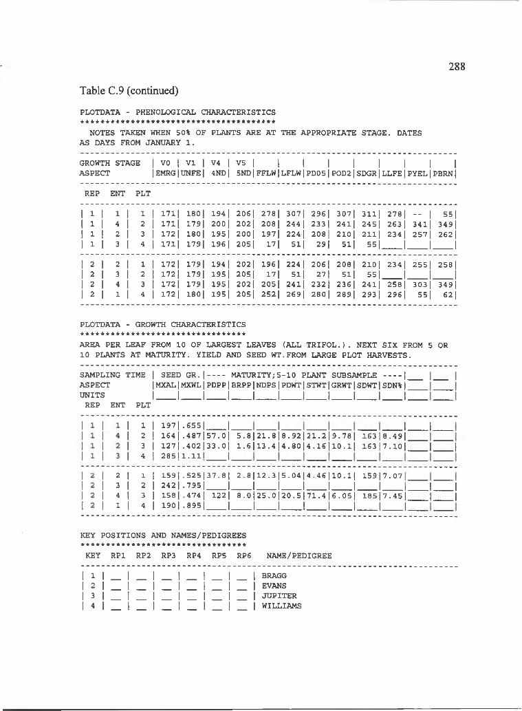
288
PLOTDATA - PHENOLOGICAL CHARACTERISTICS
NOTES TAKEN WHEN 50% OF PLANTS ARE AT THE APPROPRIATE STAGE. DATES AS DAYS FROM JANUARY 1 .
GROWTH STAGE | VO | VI | V4 | V5 | | | | | | | | |ASPECT |EMRG|UNFE| 4ND| 5NDjFFLWjLFLWjPDO5 jP0D2jSDGRjLLFEjPYELjPBRNj
Table C.9 (continued)
REP ENT PLT
1 1 1 1 1 1 1 1711 180 1 194 1 206| 278 1 307| 296 1 307| 311| 278| - 1 55 11 1 1 4 1 2 1 1711 179| 200| 202 1 208 I 244| 233 I 241| 245| 263 1 341| 349|1 1 1 2 1 3 11 172 1 180| 195| 200| 1971 224 I 208| 210 I 211| 234| 257| 262|1 1 1 3 I 4 11 1711 179| 196| 205| 17 1 511 29| 51| 55 1 1 1 1
1 2 1 2 1 1 1I 172 1 179| 194 1 202 1 196 1 224 1 206 1 208| 210| 234 1 255| 258|1 2 1 3 1 2 11 1721 179| 195| 205| 17 1 511 27| 511 55 1 1 J, 11 2 1 4 1 3 11 1721 179| 195 I 202| 205| 2411 232 1 236 1 241| 258 1 303 1 349|1 2 1 1 1 4 11 1721 180| 195| 205| 2521 269| 280| 289| 293 I 296 1 55| 62 1
PLOTDATA - GROWTH CHARACTERISTICS * * * * * * * * * * * * * * * * * * * * * * * * * * * * * * * * *AREA PER LEAF FROM 10 OF LARGEST LEAVES (ALL T R I F O L . ) . NEXT S IX FROM 5 OR 10 PLANTS AT MATURITY. YIELD AND SEED WT.FROM LARGE PLOT HARVESTS.
SAMPLING TIME | SEED GR. | MATURITY; 5 - 1 0 PLANT SUBSAM PLE |_ASPECT IMXAL|MXWL j PDPP|BRPP|NDPS|PDWT|STWT|GRWT|SDWT|SDN% j'u n i t s I I I I I I I 1 I I i;
REP ENT PLT
1 I 197 | .6 5 5 | I2 I 164| .487| 57 .0|3 I 127| .402| 33 .0|4 I 2 8 5 1 1 .I l l I
5 .8 | 2 1 .8 | 8 .9 2 | 2 1 .2 | 9 .7 8 | 1 . 6 j l 3 .4 | 4 .8 0 | 4 .1 6 | l0 . l|
163 I 8 .4 9 | . 163 |7.10|^
.1 I.
J ___ I
234 1
1 I 159| .5 2 5 | 3 7 .8 | 2 . 8 |1 2 . 3 |5 . 0 4 |4 . 4 6 |1 0 . 1 | 159|7.07|2 I 2 4 2 | .7 9 5 | ____ |______|______|______j______|______j______|______|3 I 158|.474| 122| 8 . 0 |2 5 .0 |2 0 . 5 |7 1 . 4 |6 . 0 5 | 185|7.45|4 I 19 0 | .8 9 5 | ____ I______I______I______I______I______I_____ 1______I
J IJ I
KEY POSITIONS AND NAMES/PEDIGREES * * * * * * * * * * * * * * * * * * * * * * * * * * * * * * * * *
KEY RPl RP2 RP3 RP4 RP5 RP6 NAME/PEDIGREE
| l | _ l _ t _ l _ l _ l _ l BRAGG | 2 | _ | _ | _ | _ | _ | _ | EVANS | 3 | _ 1 _ | _ | _ | _ | _ | JUPITER | 4 | _ | _ | _ | _ | _ | _ | WILLIAMS

IBSNAT REDUCED DATA SET FOR MODELLING CROP GROWTH AND DEVELOPMENT PLOTDATA REQUIRED FOR FIELD EXPERIMENTS
GENERAL
289
Table C.IO Soybean data from Kuiaha Experiment Site, 20 h photoperiod treatment.
PERSONNELRESEARCHER:INSTITUTION:
R ich a rd O gosh i IBSNAT
EXPERIMENT TITLE: ID :
IBSNAT DAYLENGTH;SUMMER;SOYBEANS 1989 IDSS89K4
TREATMENTSGENOTYPES: 4MANAGEMENT: 1
LOCATIONNAME: KUIAHA
PLOTS** * * *
PLANTING DATE
PLANT DENSITY (PLANTS/M2)
ORGANISATIONNO.OF ROWS ( # ) :ROW LENGTH (M ):ROW SPACING (CM ): ORIENTATION OF ROWS: ALONG OR ACROSS DRAINS: SPACE BETWEEN PLOTS (CM) GROSS AREA ( M 2 ) :
June 1 6 , 1989
B r a g g /E v a n s ,3 3 . 3 ; J u p i t e r /W i l l i a m s ,2 2 .2
B ra gg /E v a n s , 2 ; J u p i t e r /W i l l ia m s , 1 3B r a g g /E v a n s ,7 5 ;J u p i t e r /W i l l i a m s ,1 1 2 .5E-Wn .a .04 .5
HARVESTNO.OF ROWS:ROW LENGTH (M ): AREA ( M 2 ) : METHOD:
10 .4B r a g g /E v a n s ,0 . 3 ; J u p i t e r /W i l l i a m s ,0 .4 5 hand
RANDOMIZATION/REPLICATIONDESIGN: RCBNO.OF REPS.-SOWN: 2
-HARVESTED: 2
PROBLEMS
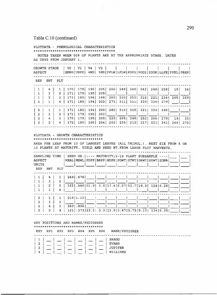
290
Table C.IO (continued)
PLOTDATA - PHENOLOGICAL CHARACTERISTICS ***************************************
NOTES TAKEN WHEN 50% OF PLANTS ARE AT THE APPROPRIATE STAGE. DATES AS DAYS FROM JANUARY 1 .
GROWTH STAGE 11 VO 1 V3 1 V4 1 V5 1 1 1 1 1 1 1 1 1ASPECT 1IEMRG1UNFE| 4ND| 5ND|FFLW|LFLW|PD05| P0D2| SDGR| l l f e |PYEL| PBRN]
REP ENT PLT
1 3 1 4 1 3 11 3701 179 1 196 1 205| 226| 248 1 240 1 243 1 248| 258| 39| 24 11 3 I 3 1 2 11 371| 179 1 195 1 205 I J 1 1 1 1 1 1 11 3 1 2 1 3 11 373 1 180 I 194 1 198 I 200| 230| 212| 216 1 221| 234| 265| 269|1 3 1 1 I 4 11 3711 180 I 194 I 202 I 273 1 331| 331| 320| 324 1 279| 1 1
1 2 1 1 1 3 i1 3711 180 1 194 1 200 1 280| 310 1 315| 32l| 324 1 290| 1 J1 2 1 3 2 11 1711 179| 195 I 202 j 1 1 1 1 1 1 1 11 2 1 4 1 3 1 1701 179 I 195| 205| 229| 265 1 248| 252 1 266 1 279| 39| 33|I 2 1 2 I 4 11 372 1 180| 195 I 204 1 202 I 2351 212 1 2171 221| 241| 268{ 272 1
PLOTDATA - GROWTH CHARACTERISTICS * * * * * * * * * * * * * * * * * * * * * * * * * * * * * * * * *AREA PER LEAF FROM 10 OF LARGEST LEAVES (ALL T R IF O L .). NEXT SIX FROM 5 OR 10 PLANTS AT MATURITY. YIELD AND SEED WT.FROM LARGE PLOT HARVESTS.
SAMPLING TIME | SEED GR. | MATURITY; 5 -1 0 PLANT SUBSAMPLE |ASPECT IMXAL|MXWL j PDPP|BRPP|NDPS|PDWT|STWT|GRWT|SDWT|SDN% ju n it s I I I I I I I I I I I
REP ENT PLT
249| .878| ______I. 1 _ _ _ _ L
162 I .540 I 5 1 .9 I 3 .6 11 7 .4 I 6 .5 7 11 2 .7 I 1 0 .9 I I 1 I I I I 1 I
I____I. I____I.124|6.26|
I____L1 I 2 1 0 | 1 .1 3 | _____ I2 I I_____ I____I3 I 260| .896| ______I4 1 121| .373| 23 .3|
J ____I.J ____I.
3 . 3 I 1 3 .6 I 3 .4 7 I 5 .7 2 I 5 .1 3 I 1 3 4 |6 . 2 5 |.1 I
KEY POSITIONS AND NAMES/PEDIGREES * * * * * * * * * * * * * * * * * * * * * * * * * * * * * * * * *
KEY RPl RP2 RP3 RP4 RP5 RP6 NAME/PEDIGREE
I 1 I 2 I 3 I 4
I _ IBRAGGEVANSJUPITERWILLIAMS

291
APPENDIX D Soybean data, summer 1990
Table D.l Soybean data from Haleakala Experiment Station, control photoperiod treatment.
IBSNAT REDUCED DATA SET FOR MODELLING CROP GROWTH AND DEVELOPMENT PLOTDATA REQUIRED FOR FIELD EXPERIMENTS
GENERAL
PERSONNELRESEARCHER:INSTITUTION:
R ich a rd O gosh i IBSNAT
EXPERIMENT TITLE: ID :
IBSNAT DAYLENGTH/SUMMER;SOYBEANS 1990 IDSS90H0
TREATMENTSGENOTYPES: 4MANAGEMENT: 0
LOCATIONNAME; HALEAKALA
PLOTS* * * * *
PLANTING DATE
PLANT DENSITY (PLANTS/M2)
J u ly 2 , 1990
33 .3
ORGANISATIONNO.OF ROWS ( # ) : 2ROW LENGTH (M ): 3ROW SPACING (CM ): 75ORIENTATION OF ROWS: E-WALONG OR ACROSS DRAINS: n .a .SPACE BETWEEN PLOTS (CM ): 0GROSS AREA ( M 2 ) : 4 .5
HARVESTNO.OF ROWS: ROW LENGTH (M) AREA ( M 2 ) : METHOD:
10 .40 .3hand
RANDOMIZATION/REPLICATIONDESIGN: RCBNO.OF REPS.-SOWN: 2
-HARVESTED: 2
PROBLEMS
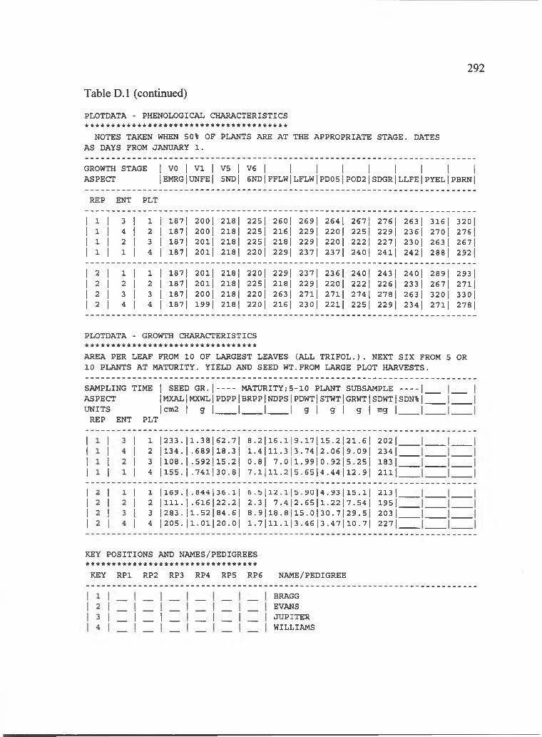
292
PLOTDATA - PHENOLOGICAL CHARACTERISTICS
Table D.l (continued)
NOTES TAKEN WHEN 50% OF PLANTS ARE AT THE APPROPRIATE STAGE. DATES AS DAYS FROM JANUARY 1 .
GROWTH STAGE | VO | V I | V5 j V6 | | | | | | | | |ASPECT |EMRG|UNFE| 5ND| 6NDjFFLW|LFLWjPDO5 jP0D2jSDGRjLLFEjPYELjPBRNj
REP ENT PLT
1 1 1 3 1 1 1 1871 200| 218 1 225 1 260| 269| 264 1 267| 276 1 263 1 316 1 320|1 1 1 4 1 2 1 1871 200| 218| 225 1 216| 229| 220 I 2251 229 I 236 1 270 I 276 I1 1 1 2 I 3 1 187| 201| 218 I 225| 218| 229| 220 1 222 1 227| 230 I 263 I 267|1 1 1 1 1 4 1 187| 20l| 218 1 220 I 229| 237| 237| 240 I 241| 242 1 288 I 292)
1 3 1 1 1 1 1 187| 20l| 218 1 220 1 229| 237| 236 1 240| 243 1 240| 289| 293 11 2 1 2 I 2 1 187| 20l| 218 I 225| 218| 229| 220 1 222 I 226 1 2331 267| 271)1 3 1 3 I 3 1 187| 200| 218 1 220 1 263 I 2711 271| 274 1 278 I 263| 320 330|1 2 j 4 1 4 1 187| 199 I 218 I 220 1 216| 230| 221| 225 1 229| 234| 271| 278 I
PLOTDATA - GROWTH CHARACTERISTICS * * * * * * * * * * * * * * * * * * * * * * * * * * * * * * * * *AREA PER LEAF FROM 10 OF LARGEST LEAVES (ALL T R I F O L . ) . NEXT SIX FROM 5 OR 10 PLANTS AT MATURITY. YIELD AND SEED WT.FROM LARGE PLOT HARVESTS.
SAMPLING TIME | SEED GR. | MATURITY; 5 - 1 0 PLANT SUBSAM PLE |ASPECT IMXAL|MXWL|PDPP|BRPP|NDPS|PDWT|STWT|GRWT|SDWT|SDN% jUNITS I cm2 I g | _____ | ______| | g | g | g | mg | ______ |
REP ENT PLT
1 | 2 3 3 .| 1 .3 8 | 6 2 .7 | 8 . 2 11 6 .1 19 .1 7 11 5 .2 |2 1 . 6 | 202|_2 |134.I .689| 18 .3| 1 . 4 j 1 1 .3 |3 . 7 4 |2 . 0 6 j 9 . 0 9 j 234|^3 | 1 0 8 .I .5 9 2 | 1 5 .2 | 0.8| 7 . 0 |1 . 9 9 j 0 .9 2 j 5 . 2 5 j 183|^4 |155. I .7 4 l| 3 0 .8 l 7 . 1 j 1 1 .2 j 5 . 6 5 |4 . 4 4 j 1 2 . 9 j 2 1 l| '
1 I 169. 1 .844 I 3 6 . 1 1 6 . 5 [ 1 2 . 1 15 . 9 0 |4 . 9 3 |1 5 . 1 1 213l_2 j l l l . I . 6 1 6 | 2 2 . 2 | 2 .3| 7 . 4 j 2 . 6 5 j 1 . 2 2 j 7 . 5 4 | 195|'3 | 2 8 3 . | 1 . 5 2 | 8 4 . 6 | 8 . 9 j 1 8 . 8 11 5 . 0 j 3 0 . 7 j 2 9 . 5 j 203 | ^4 | 2 0 5 .| 1 .0 1 | 2 0 .0 | 1 .7 | 1 1 .1 | 3 .4 6 | 3 .4 7 | 1 0 .7 | 227|'
KEY POSITIONS AND NAMES/PEDIGREES * * * * * * * * * * * * * * * * * * * * * * * * * * * * * * * * *
KEY RPl RP2 RP3 RP4 RP5 RP6 NAME/PEDIGREE
I _ I I _ I
BRAGGEVANSJUPITERWILLIAMS

293
IBSNAT REDUCED DATA SET FOR MODELLING CROP GROWTH AND DEVELOPMENT PLOTDATA REQUIRED FOR FIELD EXPERIMENTS
GENERAL
Table D.2 Soybean data from Haleakala Experiment Station, natural photoperiodtreatment.
PERSONNELRESEARCHER:INSTITUTION:
R ich a rd O gosh i IBSNAT
EXPERIMENT TITLE: ID :
IBSNAT DAYLENGTH;SUMMER/SOYBEANS 1990 IDSS90H1
TREATMENTSGENOTYPES: 4MANAGEMENT: 0
LOCATIONNAME: HALEAKALA
PLOTS* * * * *
PLANTING DATE
PLANT DENSITY (PLANTS/M2)
J u ly 2 , 1990
33 .3
ORGANISATIONNO.OF ROWS ( # ) : 2ROW LENGTH (M ): 3ROW SPACING (CM ): 75ORIENTATION OF ROWS: E-WALONG OR ACROSS DRAINS: n .a .SPACE BETWEEN PLOTS (CM ): 0GROSS AREA ( M 2 ) : 4 .5
HARVESTNO.OF ROWS: ROW LENGTH (M) AREA (M 2 ) : METHOD:
10 .40 .3hand
RANDOMIZATION/REPLICATIONDESIGN: RCBNO.OF REPS.-SOWN: 2
-HARVESTED: 2
PROBLEMS********
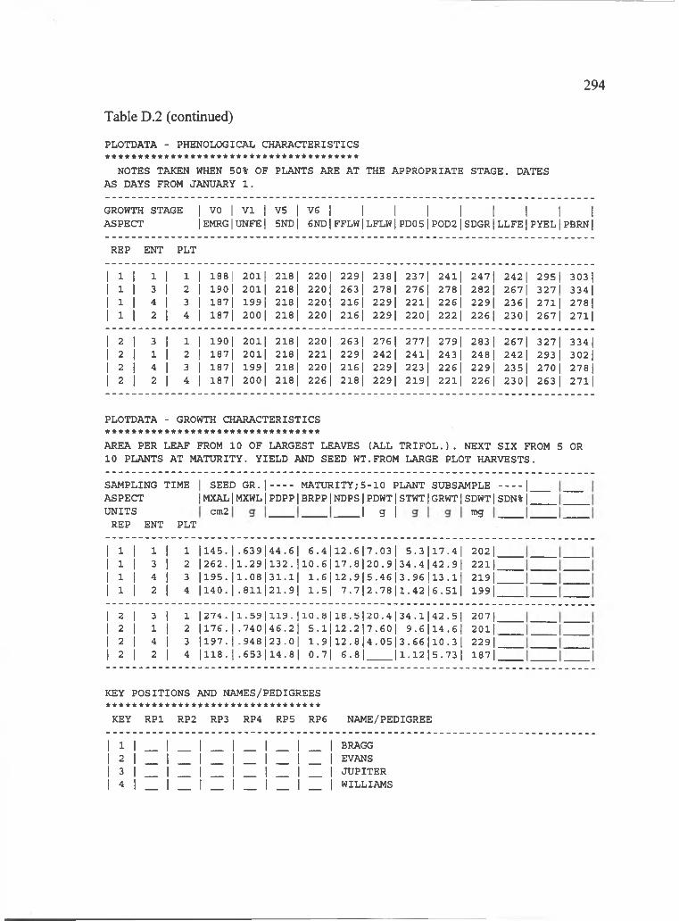
294
Table D.2 (continued)
PLOTDATA - PHENOLOGICAL CHARACTERISTICS ***************************************
NOTES TAKEN WHEN 50% OF PLANTS ARE AT THE APPROPRIATE STAGE. DATES AS DAYS FROM JANUARY 1 .
GROWTH STAGE 1 VO 1 VI 1 V5 1 V6 1 1 1 1 1 1 1 1 1ASPECT 1EMRG| UNFE| 5ND| 6ND| FFLW ILFLW| PD05| P0D2| SDGR| LLFE 1PYELl PBRN|
REP ENT PLT
1 1 1 1 1 1 1 188 1 201| 218 1 220 1 229| 238| 237| 24l| 247| 242 1 295| 303 11 1 1 3 1 2 1 190 11 201| 218 1 220| 263 1 278 1 276 1 278| 282 1 267| 3271 334|1 1 1 4 1 3 1 187 1! 1991 218 1 220| 216 1 229| 22l| 226 1 229| 236| 271| 278 11 1 1 2 1 4 1 187|1 200| 218| 220| 216 1 229| 220 1 222 1 226 1 230| 267| 271|
1 2 I 3 1 1 1 190 11 201| 218| 220 1 263 1 276 1 277 1 279| 283 I 267| 327| 334 11 2 1 1 1 2 1 187|1 201| 218 1 221| 229| 242 1 24l| 243 1 248| 242 1 293 1 302|1 2 1 4 1 3 1 187|1 1991 218 1 220 1 216| 229| 223 1 226 1 229 1 235| 270 1 278|1 2 I 2 1 4 1 187|1 200| 218| 226 1 218 I 229| 219| 221| 226 1 230| 263 1 271|
PLOTDATA - GROWTH CHARACTERISTICS * * * * * * * * * * * * * * * * * * * * * * * * * * * * * * * * *AREA PER LEAF FROM 10 OF LARGEST LEAVES (ALL T R IF O L .). NEXT SIX FROM 5 OR 10 PLANTS AT MATURITY. YIELD AND SEED WT.FROM LARGE PLOT HARVESTS.
SAMPLING TIMEASPECTUNITS
I SEED G R .] MATURITY;5-10 PLANT SUBSAMPLE -------- |IMXAL1MXWL1PDPP|BRPP|NDPS|PDWT|STWT|GRWT|SDWT|SDN%|
cm2 .1 g I mgR E P E N T P L T
1 1 1 1 1 |145. 1-639||44.6| 6 .4 | 1 2 .6 | 7 .0 3 1 5.3||17.4| 202 11 1 3 1 2 |262. |1.29|1132.1 1 0 .6| 17 .8|20 .9| 34 .4 1|42.9| 221|1 1 4 1 3 1195. |1.08||31.1| 1 .6 1 1 2 .9|5 .46| 3 .9 6 |13.1| 219|1 1 2 1 4 |140. 1.8111|21.9| 1.5| 7 .7|2 .78| 1 .4 2 |6.51| 199|
2 1 3 1 1 1 27 4 . |1.59|1119-1 1 0 . 8 1 1 8 .5|20 .4| 3 4 .1||42.5| 207|2 1 1 1 2 |176. 1 -740||46.2| 5 .1 | 12 .2|7 .60| 9.6|114.61 201|2 1 4 1 3 1 197 . 1 .9 4 8 j|23.0| 1 .9 | 12 .8|4 .05| 3.66||10.31 229|2 1 2 1 4 1 118 . 1 -6531114.81 0.7| 6 •8| 11.12115.731 187|
KEY POSITIONS AND NAMES/PEDIGREESA * * * * * * * * * * * * * * * * * * * * * * * * * * * * * * * *
KEY RPl RP2 RP3 RP4 RP5 RP6 NAME/PEDIGREE
| l | _ l _ l _ l _ l _ l _ l BRAGG | 2 | _ | _ | _ | _ | _ 1 _ | EVANS | 3 | _ | _ | _ | _ | _ | _ | JUPITER l 4 | __ I I 1 1 I __ 1 WILLIAMS

295
IBSNAT REDUCED DATA SET FOR MODELLING CROP GROWTH AND DEVELOPMENT PLOTDATA REQUIRED FOR FIELD EXPERIMENTS
GENERAL* * * * * * *
PERSONNELRESEARCHER: R ich a rd O gosh iINSTITUTION: IBSNAT
EXPERIMENTTITLE: IBSNAT DAYLENGTH;SUMMER;SOYBEANS 1990ID : IDSS90H2
TREATMENTSGENOTYPES: 4MANAGEMENT: 0
LOCATIONNAME: HALEAKALA
Table D.3 Soybean data from Haleakala Experiment Station, 14 h photoperiodtreatment.
PLOTS*****
PLANTING DATE J u ly 2 , 1990
PLANT DENSITY (PLANTS/M2) 3 3 .3
ORGANISATIONNO.OF ROWS ( # ) : 2ROW LENGTH (M ): 3ROW SPACING (CM ): 75ORIENTATION OF ROWS: E-WALONG OR ACROSS DRAINS: n .a .SPACE BETWEEN PLOTS (CM ): 0GROSS AREA ( M 2 ) : 4 .5
HARVESTNO.OF ROWS: 1ROW LENGTH (M ): 0 .4AREA ( M 2 ) : 0 .3METHOD: hand
RANDOMIZATION/REPLICATIONDESIGN: RCBNO.OF REPS.-SOWN: 2
-HARVESTED: 2
PROBLEMS********
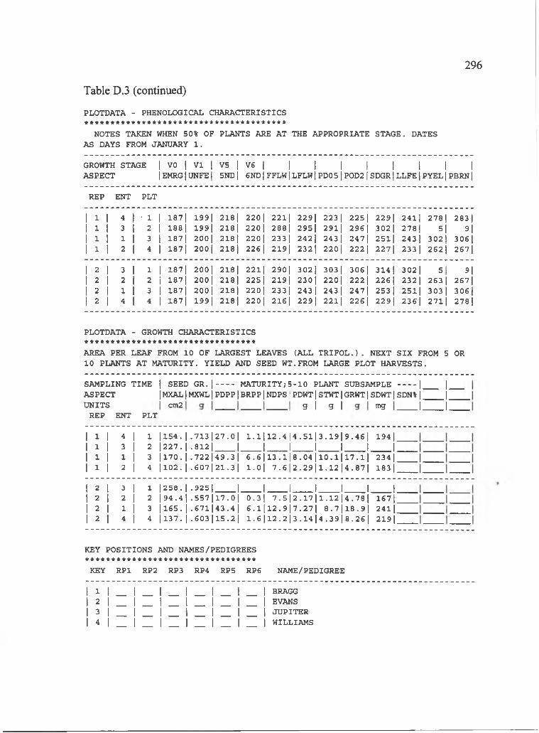
296
Table D.3 (continued)
PLOTDATA - PHENOLOGICAL CHARACTERISTICS ***************************************
NOTES TAKEN WHEN 50% OF PLANTS ARE AT THE APPROPRIATE STAGE. DATES AS DAYS FROM JANUARY 1 .
GROWTH STAGE 11 VO 1 V3 1 V5 1 V6 1 1 1 1 1 1 1 1 1ASPECT 1EMRG| UNFEl 5NDl 6NDl FFLW1LFLW1PD051P0D21SDGR1LLFE1PYELl PBRNl
REP ENT PLT
1 3 1 4 1 • 3 !1 387| 1991 218 1 220 1 2211 2291 223 1 2251 2291 2 4 ll 278 1 283 11 3 1 3 1 3 11 388 1 199 I 218 I 220 I 2881 295| 2911 2961 302| 2781 5| 9|I 3 1 1 I 3 11 387| 200 1 218 1 220 I 2331 242| 243 I 247 1 2511 243 1 3021 306 11 3 I 3 1 4 11 3871 200 I 218| 226 1 219| 2321 220 I 222 I 2271 233 1 262| 267|
1 3 1 3 1 3 1 3871 2001 218 1 2211 2901 3021 303 1 3061 314 1 3021 51 9|1 3 1 3 1 3 1 387 1 200| 218 I 2251 219 1 230j 220 1 222 1 226 I 232 1 263 1 26711 3 1 1 1 3 1 3871 200| 218 1 2201 233 1 243 I 243 I 2471 253 1 251| 303 1 306 j1 3 1 4 1 4 1 3871 199 I 218 I 2 2 oj 216 I 229| 2211 226| 2291 236| 2711 278 I
PLOTDATA - GROWTH CHARACTERISTICS * * * * * * * * * * * * * * * * * * * * * * * * * * * * * * * * *AREA PER LEAF FROM 10 OF LARGEST LEAVES (ALL T R IF O L .). NEXT SIX FROM 5 OR 10 PLANTS AT MATURITY. YIELD AND SEED WT.FROM LARGE PLOT HARVESTS.
SAMPLING TIMEASPECTUNITS
1 SEED G R .| MATURITY;5-10 PLANT SUBSAMPLE ------- |____ |_IMXALIMXWLIPDPP|BRPP|NDPS|PDWT|STWT|GRWT|SDWT|SDN% j______j'
cm2 g I g I mg J I.REP ENT PLT
1 1 4 1 1 1154.1 .7 1 3 1 2 7 .0 1 1 .1 1 1 2 .4 l 4 . 5 l l 3 . 1919 .461 194 11 1 3 1 2 1227.1 .8121 1 1 .... ..J 1 1 1 1 11 1 1 1 3 1170.1 .7 2 2 1 4 9 .3 1 6 .6 1 1 3 .1 | 8 . 0 4 l l 0 . l l l 7 . l l 234 11 1 2 1 4 1102.1 .6 0 7 1 2 1 .3l l . o j 7 .6 2 .2 9 | 1 .1 2 | 4 .8 7 | 183 1
2 1 3 1 1 1258.1 .9251 1 1 1 1 1 1 12 1 2 1 2 194.41 .5 5 7 1 1 7 .0 1 0 .31 7 .5 I 2 . 1 7 l l . l 2 l 4 . 7 8 l 16712 1 1 I 3 1165.1 .6 7 1 | 4 3 .4 I 6 .1 1 1 2 .9 |7.27| 8 .7 | l 8 .9 l 24l|2 I 4 1 4 1137.1 .603| 15 .2| 1 .6 112 .2 | 3 .1 4 | 4 .3 9 | 8 .2 6 | 219|
KEY POSITIONS AND NAMES/PEDIGREES * * * * * * * * * * * * * * * * * * * * * * * * * * * * * * * * *
KEY RPl RP2 RP3 RP4 RP5 RP6 NAME/PEDIGREE
l l | _ l _ l _ l _ l _ l _ l BRAGG | 2 | _ | _ | _ 1 _ 1 _ | _ | EVANS | 3 | _ l _ l _ l _ l _ l _ l JUPITER | 4 | _ | _ | _ | _ | _ | _ | WILLIAMS

297
IBSNAT REDUCED DATA SET FOR MODELLING CROP GROWTH AND DEVELOPMENT PLOTDATA REQUIRED FOR FIELD EXPERIMENTS
GENERAL
Table D.4 Soybean data from Haleakala Experiment Station, 17 h photoperiodtreatment.
PERSONNELRESEARCHER: INSTITUTION:
R ich a rd O gosh i IBSNAT
EXPERIMENT TITLE: ID :
IBSNAT DAYLENGTH/SUMMER/SOYBEANS 1990 IDSS90H3
TREATMENTSGENOTYPES: 4MANAGEMENT: 0
LOCATIONNAME: HALEAKALA
PLOTS*****
PLANTING DATE
PLANT DENSITY (PLANTS/M2)
J u ly 2 , 1990
3 3 .3
ORGANISATIONNO.OF ROWS ( # ) : 2ROW LENGTH (M ): 3ROW SPACING (CM ): 75ORIENTATION OF ROWS: E-WALONG OR ACROSS DRAINS: n .a .SPACE BETWEEN PLOTS (CM ): 0GROSS AREA ( M 2 ) : 4 .5
HARVESTNO.OF ROWS: ROW LENGTH (M) AREA ( M 2 ) : METHOD:
10 .40 .3hand
RANDOM IZATI ON/REPLI CAT I ONDESIGN: RCBNO.OF REPS.-SOWN: 2
-HARVESTED: 2
PROBLEMS********
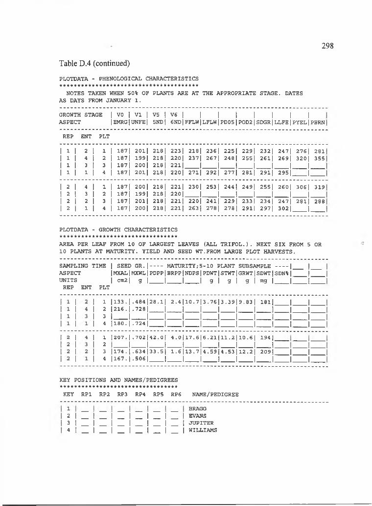
298
PLOTDATA - PHENOLOGICAL CHARACTERISTICS
NOTES TAKEN WHEN 50% OF PLANTS ARE AT THE APPROPRIATE STAGE. DATES AS DAYS FROM JANUARY 1 .
Table D.4 (continued)
GROWTH STAGE 1 VO 1 VI 1 V5 1 V6 1 1 1 1 1 1 1 1ASPECT 1EMRGl UNFE I 5ND1 6ND1FFLW1LFLW1PDO 5 |P0D21SDGR1LLFE|PYEL1PBRN
REP ENT PLT
1 3 1 2 1 1 1 1871 2011 2181 223 1 2181 236 1 2251 2291 232 1 2471 276 1 2811 3 1 4 1 2 1 187| 199 1 218 1 220 1 2371 267| 248 I 2551 26l| 269| 320| 3551 I 1 3 1 3 1 1871 200 I 218 I 2 2 1 1 1 1 1 1 1 1 J1 I 1 1 I 4 1 1871 201| 218 1 2201 2711 2921 277 1 2811 2911 2951 1
1 2 1 4 1 1 1 187| 200 1 218 1 2211 2301 253 1 244 1 2491 2551 2601 306 1 3191 2 1 3 1 2 1 187| 199| 218| 220 1 1 1 1 1 1 J 11 2 1 2 1 3 1 1871 201| 218| 2211 2201 2411 229| 233 1 234 1 2471 2811 2881 2 1 1 1 4 1 1871 200| 218| 221| 2631 278 I 278 1 2911 2971 302| 1
PLOTDATA - GROWTH CHARACTERISTICS * * * * * * * * * * * * * * * * * * * * * * * * * * * * * * * * *AREA PER LEAF FROM 10 OF LARGEST LEAVES (ALL T R IF O L .). NEXT SIX FROM 5 OR 10 PLANTS AT MATURITY. YIELD AND SEED WT.FROM LARGE PLOT HARVESTS.
SAMPLING TIME | SEED G R .|------- MATURITY;5 -1 0 PLANT SUBSAMPLE --------|____ |ASPECT IMXAL|MXWL j PDPP|BRPP|NDPS|PDWT|STWT|GRWT[SDWT|SDN% j j'UNITS I cm2 I g |______|______|______ | g | g 1 g | mg |______|______f
REP ENT PLT
1 |133.I.484|28.1| 2 .4|10.7|3.76|3.39|9.83| 18lj2___ | 2 1 6 .| .7 2 8 | ____ I______I______I______I______I______I_____ 13 I I I I I I I I I I4___ 1 1 8 0 .| .7 2 4 | ____ I______I______I______I______I______I_____ I
J ____ I.J ____ I.J ____ I..1____ I.
1 | 2 0 7 . I . 7 0 2 | 4 2 . 0 | 4 . 0 |1 7 . 6 1 6 . 2 1 |1 1 . 2 |1 0 . 6 | 1 9 4 |
2 1 I I I I 1 I I I 13 |174.I.634|33.5| 1 .6|13.7|4.59|4.53|12.2| 209|4 |167. 1 .5 0 6 1 I I 1 I 1_____ 1______I
J ____ I.J ____ I.
KEY POSITIONS AND NAMES/PEDIGREES * * * * * * * * * * * * * * * * * * * * * * * * * * * * * * * * *
KEY RPl RP2 RP3 RP4 RP5 RP6 NAME/PEDIGREE
BRAGG2 | _ l _ l _ l _ l _ l _ l EVANS3 l __ 1 1 1 1 1 1 JUPITER4 | __ I I I I 1 1 WILLIAMS
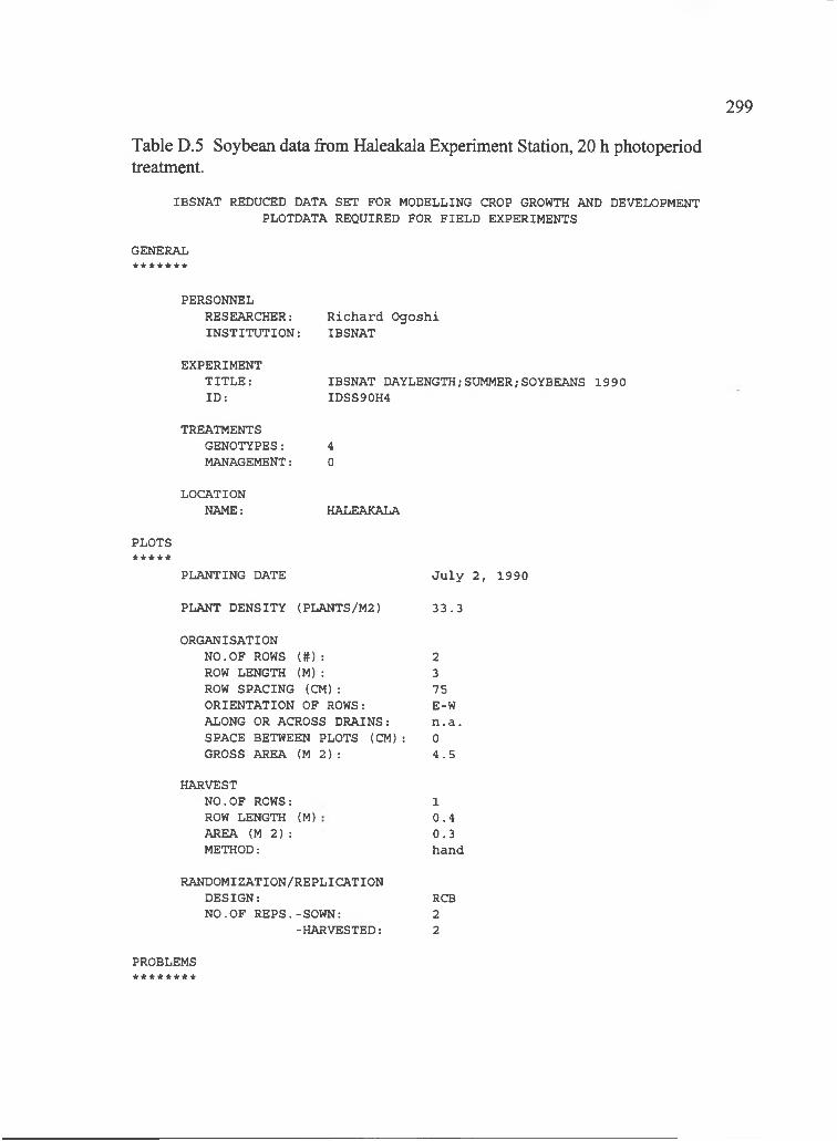
299
IBSNAT REDUCED DATA SET FOR MODELLING CROP GROWTH AND DEVELOPMENT PLOTDATA REQUIRED FOR FIELD EXPERIMENTS
GENERAL
Table D.5 Soybean data from Haleakala Experiment Station, 20 h photoperiodtreatment.
PERSONNELRESEARCHER:INSTITUTION:
R ich a rd O gosh i IBSNAT
EXPERIMENT TITLE: ID :
IBSNAT DAYLENGTH/SUMMER/SOYBEANS 1990 IDSS90H4
TREATMENTSGENOTYPES: 4MANAGEMENT: 0
LOCATIONNAME: HALEAKALA
PLOTS* * * * *
PLANTING DATE
PLANT DENSITY {PLANTS/M2)
J u ly 2 , 1990
3 3 .3
ORGANISATIONNO.OF ROWS ( # ) : 2ROW LENGTH (M ): 3ROW SPACING (CM ): 75ORIENTATION OF ROWS: E-WALONG OR ACROSS DRAINS: n .a .SPACE BETWEEN PLOTS (CM ): 0GROSS AREA ( M 2 ) : 4 .5
HARVESTNO.OF ROWS: ROW LENGTH (M) AREA ( M 2 ) : METHOD:
10 .40 .3hand
RANDOMIZATION/REPLICATIONDESIGN: RCBNO.OF REPS.-SOWN: 2
-HARVESTED: 2
PROBLEMS********

300
Table D.5 (continued)
PLOTDATA - PHENOLOGICAL CHARACTERISTICS ***************************************
NOTES TAKEN WHEN 50% OF PLANTS ARE AT THE APPROPRIATE STAGE. DATES AS DAYS FROM JANUARY 1 .
GROWTH STAGE 1 VO 1 V3 1 V5 1 V6 1 1 1 1 1 1 1 1 1ASPECT 1EMRG1UNFE| 5ND| 6ND| FFLW| LFLW| PD05| P0D2| SDGR| LLFE| PYEL| PBRN|
REP ENT PLT
1 3 1 4 1 3 1 187 1 200| 218| 222 1 249| 277 1 267| 271| 277| 269| 2| 9|1 3 I 1 I 2 1 187| 201| 218 1 223 1 316 I 330| 318| 322| 330| 327| 1 11 3 1 2 1 3 1 187| 200| 218 1 220| 2231 2411 235| 240| 243 I 261| 320| 322|1 3 I 3 I 4 1 187] 200| 218 I 225 I 1 1 1 1 1 1 1 1
1 2 1 1 1 3 1 187| 201| 218 1 220 1 291| 320| 317| 319| 330| 306 1 1 11 2 1 3 1 2 1 188 I 200 I 218 I 222 1 1 1 1 1 J 1 11 2 I 2 1 3 1 187| 199 I 218 I 221| 229| 240{ 236 1 241| 245| 260| 298 1 320|1 2 1 4 1 4 1 187| 199 I 218 I 2 2 1 1 245| 271| 257| 262| 271| 281| 2| 9|
PLOTDATA - GROWTH CHARACTERISTICS * * * * * * * * * * * * * * * * * * * * * * * * * * * * * * * * *AREA PER LEAF FROM 10 OF LARGEST LEAVES (ALL T R IF O L .). NEXT SIX FROM 5 OR 10 PLANTS AT MATURITY. YIELD AND SEED WT.FROM LARGE PLOT HARVESTS.
SAMPLING TIME | SEED G R .| ------- MATURITY;5 -1 0 PLANT SUBSAMPLE -------- |ASPECT IMXAL|MXWL j PDPP|BRPP|NDPS|PDWT|STWT|GRWT|SDWT|SDN% j 'UNITS I cm2| g 1______|______|______ | g | g | g | mg |______ |;
REP ENT PLT
| 1 7 1 .1 .560|_ | 1 61 .I .509| _
J ____ I.J ____I.
|179. I .703| 71 .2| 4 .3 | 2 1 .6 | 1 0 .5 | 2 2 .2 | 1 7 .4 | 1 9 3 jI I I I I I I 1 I !
13 24
1 |175. I .626| _I2 I___I____ I____I3 |187.I .6 8 8 j8 3 .0 |4 l l 5 1 .1 .4 4 7 | _____I
.1. .1 I.
4 .2 | 1 9 .7 | 1 1 .7 | 2 1 .5 | 1 7 .2 | I I I I I
197|
KEY POSITIONS AND NAMES/PEDIGREES * * * * * * * * * * * * * * * * * * * * * * * * * * * * * * * * *
KEY RPl RP2 RP3 RP4 RP5 RP6 NAME/PEDIGREE
| l | _ l _ l _ l _ l _ l _ l BRAGG | 2 | _ | _ | _ | _ | _ | _ | EVANS | 3 | _ | _ | _ | _ | _ | _ 1 JUPITER I 4 I I I I I I I WILLIAMS
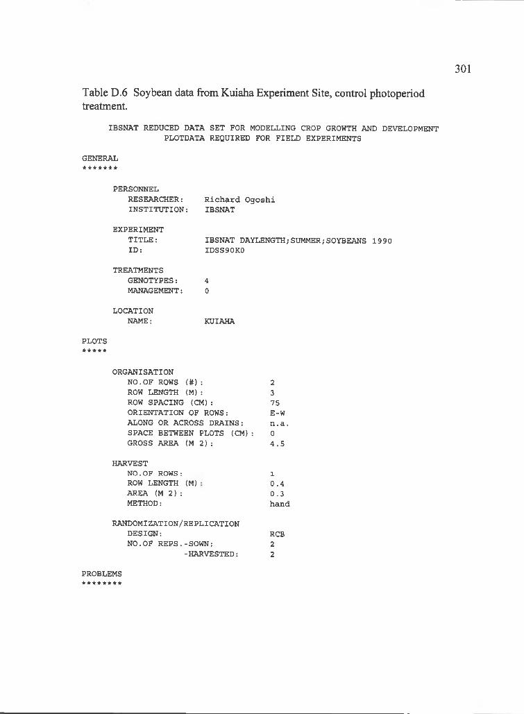
301
IBSNAT REDUCED DATA SET FOR MODELLING CROP GROWTH AND DEVELOPMENT PLOTDATA REQUIRED FOR FIELD EXPERIMENTS
GENERAL
Table D.6 Soybean data from Kuiaha Experiment Site, control photoperiodtreatment.
PERSONNELRESEARCHER:INSTITUTION:
R ich a rd O gosh i IBSNAT
EXPERIMENT TITLE: ID :
IBSNAT DAYLENGTH/SUMMER/SOYBEANS 1990 IDSS90K0
TREATMENTSGENOTYPES: 4MANAGEMENT: 0
LOCATIONNAME: KUIAHA
PLOTS* * * * *
ORGANISATIONNO.OF ROWS ( # ) : 2ROW LENGTH (M ): 3ROW SPACING (CM ): 75ORIENTATION OF ROWS: E-WALONG OR ACROSS DRAINS: n .a .SPACE BETWEEN PLOTS (CM ): 0GROSS AREA ( M 2 ) : 4 .5
HARVESTN O . O F R O W S : ROW LENGTH (M) AREA ( M 2 ) : METHOD:
1
0 .40 .3hand
RANDOMIZATION/REPLICATIONDESIGN: RCBNO.OF REPS.-SOWN: 2
-HARVESTED: 2
PROBLEMS********
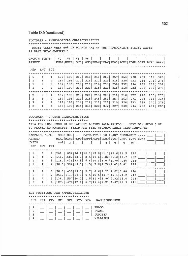
302
Table D.6 (continued)
PLOTDATA - PHENOLOGICAL CHARACTERISTICS ***************************************
NOTES TAKEN WHEN 50% OF PLANTS ARE AT THE APPROPRIATE STAGE. DATES AS DAYS FROM JANUARY 1 .
GROWTH STAGE ASPECT
I VO 1 VI 1 V5 I V6 I I I 1 I I I I I IEMRG1UNFE| 5ND| 6ND|FFLW|LFLW|PDO 5 |P0D2|SDGR j LLFE|PYEL|PBRN|
REP ENT PLT
1 1 1 3 1 1 11 187| 1951 2151 218 1 248 1 263 1 257) 263 1 270) 253 1 3121 320 11 1 1 4 I 2 !1 187| 195 I 212 1 216| 212 1 223 1 218 1 220 I 223 1 234) 2711 276 I1 1 1 1 I 3 i1 187| 196| 213 1 216| 218) 233 1 230| 2321 234 1 232 I 283 1 292 I1 1 1 2 1 4 11 187| 197| 218 1 220| 2151 2211 216 I 218 1 222 I 227| 260| 270|
1 2 1 2 1 1 11 187| 196) 218 1 220) 215 1 223 1 216 1 218 1 222 1 226 1 260 1 270)1 2 1 3 1 2 1 1871 196 1 216 I 218| 248 1 263 1 2571 263 I 2711 254 I 311| 314|1 2 1 4 I 3 11 1871 196 I 214 I 218 I 213 1 222 I 2191 220 1 223 1 234 I 270 1 276 11 2 1 1 1 4 1 188| 198 I 214 I 216 1 220 1 232 I 2271 230 I 234) 230| 281| 285 I
PLOTDATA - GROWTH CHARACTERISTICS *********************************AREA PER LEAF FROM 10 OF LARGEST LEAVES (ALL T R IF O L .). NEXT SIX FROM 5 OR 10 PLANTS AT MATURITY. YIELD AND SEED WT.FROM LARGE PLOT HARVESTS.
SAMPLING TIME | SEED G R .|------- MATURITY;5 -1 0 PLANT SUBSAMPLE -------- |ASPECT IMXAL|MXWL j PDPP|BRPP|NDPS|PDWT|STWT|GRWT|SDWT|SDN% ju n it s I cm 21 g j_______ j______j______j g j g | g | mg |______j
REP ENT PLT
1 1 3 1 1 1208. 1 .854||76.2l 1 0 .1 ) 1 5 .8 ) 1 1 .1 ) 1 8 .6 121.51 230)1 1 4 1 2 | 1 4 8 .1 .683 |28.8l 2 .5 | 1 1 .5 | 5 .0 2 | 3 .1 2 113.71 22711 1 1 1 3 1 1 1 5 .1 .4 3 1 1 3 3 .5 1 6 .6 | 1 0 .3 | 5 .0 7 | 6 .7 0 | 7 .5 6 l 21511 1 2 1 4 l9 8 .9 l .504 ]119-81 1.5| 7 . 6 | 2 .7 6 1 1 .4 2 | 8 .4 l l 197)
2 1 2 1 1 1 7 8 .6 1 .430||18.31 2 .7 ) 6 .6 1 2 .2 3 1 1 .0 2 1 7 .4 8 ) 194 12 1 3 1 2 1 2 5 1 .l l . 1 7 ) 6 9 . l l 9 . 5 | 1 5 .6 | 1 0 .7 )1 7 .1 | 2 4 .2 l 247)3 1 4 1 3 ) 1 3 6 . 1 .597 ]124.21 1 .5 | l l . 4 l 3 .8 6 | 2 .3 2 113.01 228)2 1 1 1 4 j l 2 7 . 1 .470 | 47.0 l 6 .7 ) 1 1 .4 ) 7 . 2 1 ) 4 . 4 7 ) 2 2 .9 ) 241)
J I.J I
J I
KEY POSITIONS AND NAMES/PEDIGREES * * * * * * * * * * * * * * * * * * * * * * * * * * * * * * * * *
KEY RPl RP2 RP3 RP4 RP5 RP6 NAME/PEDIGREE
| l | _ l _ l _ l _ l _ l _ l BRAGG | 2 | _ | _ | _ | _ | _ | _ | EVANS | 3 | _ 1 _ | _ | _ | _ 1 _ | JUPITER | 4 | __ I I I I I __ I WILLIAMS

303
IBSNAT REDUCED DATA SET FOR MODELLING CROP GROWTH AND DEVELOPMENT PLOTDATA REQUIRED FOR FIELD EXPERIMENTS
GENERAL
Table D.7 Soybean data from Kuiaha Experiment Site, natural photoperiodtreatment.
PERSONNELRESEARCHER:INSTITUTION:
R ich a rd O gosh i IBSNAT
EXPERIMENT TITLE: ID :
IBSNAT DAYLENGTH/SUMMER/SOYBEANS 1990 IDSS90K1
TREATMENTSGENOTYPES: 4MANAGEMENT: 0
LOCATIONNAME: KUIAHA
PLOTS* * * * *
PLANTING DATE
PLANT DENSITY (PLANTS/M2)
J u ly 2 , 1990
3 3 .3
ORGANISATIONNO.OF ROWS ( # ) : 2ROW LENGTH (M ): 3ROW SPACING (CM ): 75ORIENTATION OF ROWS: E-WALONG OR ACROSS DRAINS: n .a .SPACE BETWEEN PLOTS (CM ): 0GROSS AREA ( M 2 ) : 4 .5
HARVESTNO.OF ROWS: ROW LENGTH (M) AREA ( M 2 ) : METHOD:
10 .40 .3hand
RANDOMIZATION/REPLICATIONDESIGN: RCBNO.OF REPS.-SOWN: 2
-HARVESTED: 2
PROBLEMS********
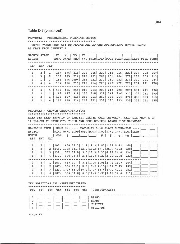
304
Table D.7 (continued)
PLOTDATA - PHENOLOGICAL CHARACTERISTICS ***************************************
NOTES TAKEN WHEN 50% OF PLANTS ARE AT THE APPROPRIATE STAGE. DATES AS DAYS FROM JANUARY 1 .
GROWTH STAGE 1 VO 1 VI 1 V5 1 V6 1 1 1 1 1 1 1 1 1ASPECT 1EMRG1UNFE| 5NDl 6NDl FFLWl LFLWl PD051P0D21SDGR1LLFE1PYEL| PBRNl
REP ENT PLT
1 3 1 2 1 1 1 187| 1961 218 1 220 1 215| 222 1 2151 2161 222 1 2271 262 1 26711 3. 1 3 I 2 1 188| 195 1 214 I 216 I 251| 2671 2 6 ll 264 1 2711 2561 309| 31311 3- 1 1 1 3 1 188 1 196 I209^ I 216 I 221| 232| 230| 233 1 234 1 230| 281| 284 11 3. 1 4 I 4 1 187| 196 I 216 1 219| 214 1 223 1 220| 222 I 228 I 234 1 2711 276 1
1 2 1 4 1 1 11 3.871 1961 216 1 2181 213 1 223 1 218 1 222 1 2271 234 1 2711 276 11 2 1 2 1 2 11 1871 197| 218 1 220| 2151 223 1 2151 2161 2221 227| 2 6 l l 269|1 2 1 3 1 3 1I 188| 197| 2151 218 I 251| 2671 2601 264 1 2711 2551 309| 31311 2 1 1 1 4 11 188| 198| 214 I 218| 22l| 232 1 230| 2331 2351 2321 28l| 2851
PLOTDATA - GROWTH CHARACTERISTICS *********************************AREA PER LEAF FROM 10 OF LARGEST LEAVES (ALL T R IF O L .). NEXT SIX FROM 5 OR 10 PLANTS AT MATURITY. YIELD AND SEED WT.FROM LARGE PLOT HARVESTS.
SAMPLING TIME | SEED G R .|------- MATURITY;5 -1 0 PLANT SUBSAMPLE -------- |_ASPECT IMXAL|MXWL j PDPP|BRPP|NDPS|PDWT|STWT|GRWT|SDWT|SDN% j 'u n i t s . 1 cm 2 1 g | _______ j______j______| g j g j g | mg j______|_
REP ENT PLT
1 |102.I .474| 26 .2| 1.9| 8 . 3 |2 . 8 3 11 . 3 2 |9 . 2 2 | 169|2 | 2 4 5 .| 1 .2 9 | 1 3 1 .| l2 .9 | l9 .3 l l7 .3 | 3 5 .7 | 4 8 .3 | 230|3 | 1 3 8 . I . 5 6 2 | 5 2 . 8 | 9 . 0 j 1 1 . 3 j 7 . 3 3 j 6 . 2 9 j 2 4 . 0 j 2 2 4 j4 |133.I .660| 24 .6| 2 . 1 11 1 .0 j 4 . 2 2 j 2 . 5 2 j 1 3 . 8 j 2 2 2 |
1 |150.I .657| 30 .7| 2 . 5 112 . 4 |5 . 0 5 |2 . 7 2 |15 . 7 | 204|_2 I 1 0 7 . I . 5 3 6 | 1 9 . 1 | 0 . 9 | 7 . 5 j 2 . 1 5 11 . 0 2 j 7 . 4 3 j 1 8 9 | '3 | 2 2 3 .| 1 .2 3 | 9 6 .2 | 1 0 .2 | 1 7 .6 | 1 3 .8 | 2 7 .0 | 4 1 .4 | 2 5 l| '4 |107. I .334| 34 .0| 6 . 6 j 1 0 .6 j 3 . 9 3 j 3 . 1 2 112 . 6 j 2 1 l| '
KEY POSITIONS AND NAMES/PEDIGREES
KEY RPl RP2 RP3 RP4 RP5 RP6 NAME/PEDIGREE
| l | _ l _ l _ l _ l _ l _ l BRAGG | 2 | _ | _ | _ | _ | _ | _ | EVANS | 3 | _ | _ | _ | _ | _ | _ | JUPITER | 4 | __ I I I I I I WILLIAMS
♦ t r u e V4

305
IBSNAT REDUCED DATA SET FOR MODELLING CROP GROWTH AND DEVELOPMENT PLOTDATA REQUIRED FOR FIELD EXPERIMENTS
Table D.8 Soybean data from Kuiaha Experiment Site, 14 h photoperiod treatment.
GENERAL
PERSONNELRESEARCHER:INSTITUTION:
R ich a rd O gosh i IBSNAT
EXPERIMENT TITLE: ID :
IBSNAT DAYLENGTH/SUMMER/SOYBEANS 1990 IDSS90K2
TREATMENTSGENOTYPES: 4MANAGEMENT: 0
LOCATIONNAME: KUIAHA
PLOTS*****
PLANTING DATE
PLANT DENSITY (PLANTS/M2)
J u ly 2 , 1990
33 .3
ORGANISATIONNO.OF ROWS ( # ) : 2ROW LENGTH (M ): 3ROW SPACING (CM ): 75ORIENTATION OF ROWS: E-WALONG OR ACROSS DRAINS: n .a .SPACE BETWEEN PLOTS (CM ): 0GROSS AREA ( M 2 ) : 4 .5
HARVESTNO.OF ROWS:ROW LENGTH (M ):AREA (M 2 ) :METHOD:
RANDOMIZATION/REPLICATIONDESIGN:NO.OF REPS.-SOWN:
-HARVESTED:
10 .40 .3hand
RCB22
PROBLEMS********
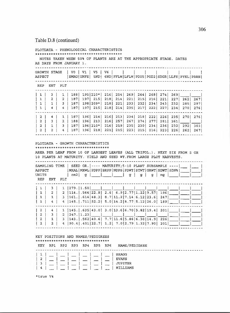
306
Table D.8 (continued)
PLOTDATA - PHENOLOGICAL CHARACTERISTICS * * * * * * * * * * * * * * * * * * * * * * * * * * * * * * * * * * * * * * *
NOTES TAKEN WHEN 50% OF PLANTS ARE AT THE APPROPRIATE STAGE. DATES AS DAYS FROM JANUARY 1 .
GROWTH STAGE 1 VO 1 VI 1 V5 1 V6 1 1 1 1 1 1 1 1 1ASPECT 1EMRG IUNFE| 5ND| 6ND| FFLWl LFLW1PD051P0D21SDGR1LLFE1PYEL|PBRN1
REP ENT PLT
1 1 1 3 1 1 1 188 1 195 1210^| 216 1 254 1 2691 264 1 2681 274 1 2691 1 11 1 1 2 1 2 1 187| 197 I 215| 218 1 214 1 2211 215 1 216| 221| 2271 2621 26711 1 1 1 I 3 1 187| 1981209^1 218 I 22l| 233 1 232 I 234 I 243 1 232 1 285 I 297|1 1 1 4 I 4 1 187 1 197| 215| 218 1 214 I 235 1 217| 222 1 227| 234 1 270 I 276 1
1 2 1 4 1 1 1i 18V| 196| 214 1 216 1 213 1 234 1 218 1 222 1 2261 2351 270 1 27611 2 1 3 1 2 11 188| 196| 213 1 216 I 2571 267| 274 I 2771 28l| 2 6 l l 1 11 2 1 1 I 3 11 187| 196| 210^1 216 1 2191 2351 230| 234 1 236 1 232| 292 1 303 11 2 1 2 1 4 11 187| 196| 218| 22l| 215 I 223 1 215 I 216| 223 I 226| 262 I 267|
PLOTDATA - GROWTH CHARACTERISTICS *********************************AREA PER LEAF FROM 10 OF LARGEST LEAVES (ALL T R IF O L .). NEXT SIX FROM 5 OR 10 PLANTS AT MATURITY. YIELD AND SEED WT.FROM LARGE PLOT HARVESTS.
SAMPLING TIME | SEED G R .[ ------- MATURITY;5 -1 0 PLANT SUBSAMPLE -------- |ASPECT IMXAL j MXWL j PDPP|BRPP|NDPS|PDWT|STWT|GRWT|SDWT|SDN% ju n i t s I cm2| g j______j______j______j g j g j g | mg j______|
REP ENT PLT
1 1 3 1 1 1279. | l .5 0 l 1 1 11 11 1 1 11 1 2 I 2 1114. 1 .5 6 4 1 2 2 .8 1 2.6|1 6.9||2.77|j l . 2219 .571 196 11 I 1 I 3 |161. I.6 1 4 | 4 8 .3 | 8.7||11.2||7.14| 6 .1 2 I 2 3 . 6 1 247|1 I 4 1 4 I l4 5 . I .7 1 l| 5 2 .2 | 5.0||14.2||8.77| 5 .1 2 | 2 6 .0 | 1891
2 1 4 1 1 1145. 1 .6 3 5 1 4 3 .0 1 3.0||13.6||6.70|| 3 .8 2 l l9 .4 l 20113 I 2 |247. 1 1 .2 3 ! 1 11 11 11 1 1 1
2 I 1 1 3 1 143 . 1 .5 6 2 1 4 0 .6 1 7 .7 j|11.6||5.86|| 6 .3 0 l l4 .9 l 226 12 1 2 1 4 l 9 0 . 4 l .4 0 1 1 2 2 .7l 1.2|1 7.0||2.79j 1 .3 2 | 7 .9 0 | 2 0 l l J I.
KEY POSITIONS AND NAMES/PEDIGREES * * * * * * * * * * * * * * * * * * * * * * * * * * * * * * * * *
KEY RPl RP2 RP3 RP4 RP5 RP6 NAME/PEDIGREE
BRAGG2 | _ l _ l _ l _ l _ l _ l EVANS3 | __ 1 I I I I 1 JUPITER4 | __ I I I I I I WILLIAMS
♦ t r u e V4

307
IBSNAT REDUCED DATA SET FOR MODELLING CROP GROWTH AND DEVELOPMENT PLOTDATA REQUIRED FOR FIELD EXPERIMENTS
Table D.9 Soybean data from Kuiaha Experiment Site, 17 h photoperiod treatment.
GENERAL
PERSONNELRESEARCHER:INSTITUTION:
R ich a rd O gosh i IBSNAT
EXPERIMENT TITLE: ID :
IBSNAT DAYLENGTH/SUMMER;SOYBEANS 1990 IDSS90K3
TREATMENTSGENOTYPES: 4MANAGEMENT: 0
LOCATIONNAME: KUIAHA
PLOTS* * * * *
PLANTING DATE
PLANT DENSITY (PLANTS/M2)
J u ly 2 , 1990
3 3 .3
ORGANISATIONNO.OF ROWS { # ) : 2ROW LENGTH (M ): 3ROW SPACING (CM ): 75ORIENTATION OF ROWS: E-WALONG OR ACROSS DRAINS: n .a .SPACE BETWEEN PLOTS (CM): 0GROSS AREA ( M 2 ) : 4 .5
HARVESTNO.OF ROWS:ROW LENGTH (M ): AREA (M 2 ) : METHOD:
10 .40 .3hand
RANDOMIZATION/REPLICATIONDESIGN: RCBNO.OF REPS.-SOWN: 2
-HARVESTED: 2
PROBLEMS********
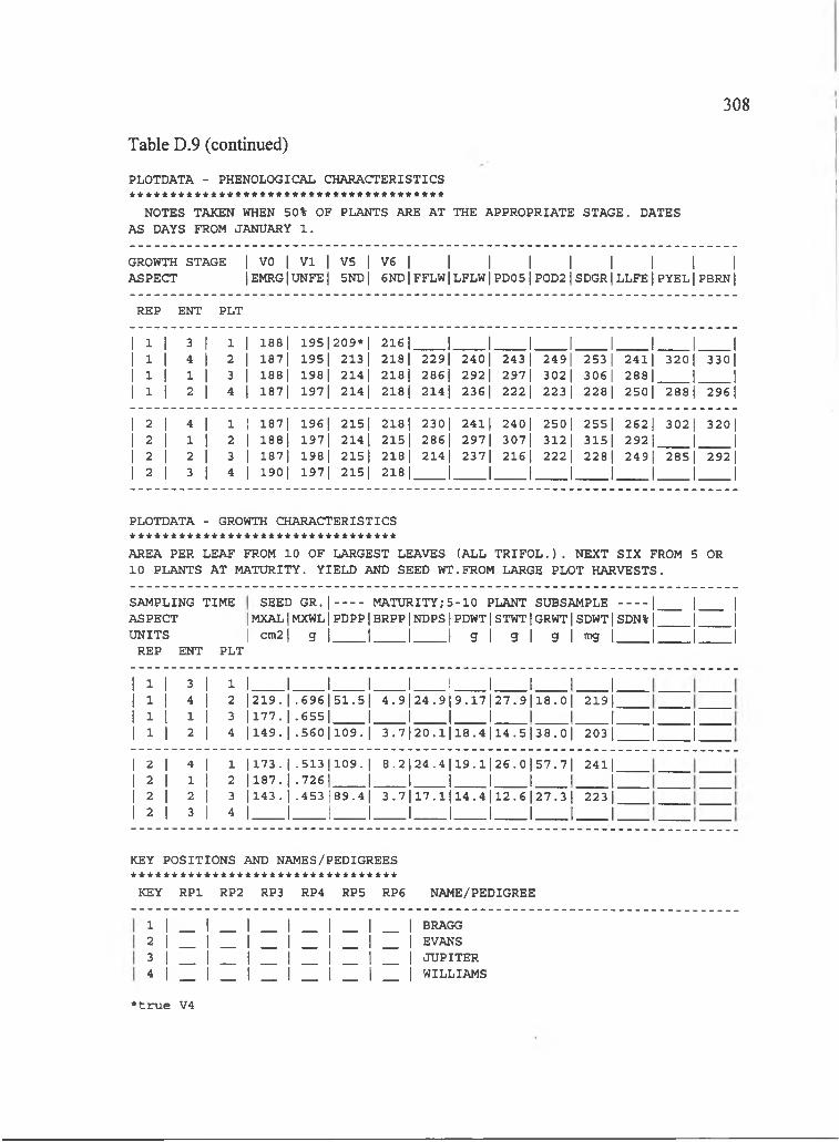
308
Table D.9 (continued)
PLOTDATA - PHENOLOGICAL CHARACTERISTICS ***************************************
NOTES TAKEN WHEN 50% OF PLANTS ARE AT THE APPROPRIATE STAGE. DATES AS DAYS FROM JANUARY 1 .
GROWTH STAGE | VO | V I | V5 | V6 | | | | | | | [ |ASPECT |EMRG|UNFE| 5ND| 6NDjFFLWjLFLWjPDO5 jP0D2jSDG RjLLFEjPYELjPBRN|
REP ENT PLT
1 1 3 1 1 11 188 1 195 1209^ 1 216 1 1 1 1 J, 1 1 1 11 1 4 1 2 11 187| 195 I 213 1 218| 229| 240 1 243 1 2491 253 1 2411 320 1 33011 1 1 I 3 11 188 1 198 I 214 1 218| 286| 292 I 297 1 3021 3061 288| 1 11 1 2 1 4 !1 187| 197 I 214 I 218| 214 I 236 1 222 I 223 1 2281 2501 2881 296 1
2 1 4 1 1 1 187| 196 1 215 1 218| 230| 2 4 l l 240| 250 1 2551 2621 3021 32012 I 1 1 2 1 188| 197 I 214 1 215| 286| 297| 307| 3121 315| 292| 1 12 1 2 1 3 1 187| 198 1 215 I 218 1 214 I 237| 2161 222 1 228 1 2491 2851 292 12 1 3 I 4 1 190| 197| 215 1 218| 1 1 1 1 1 1 1 1
PLOTDATA - GROWTH CHARACTERISTICS * * * * * * * * * * * * * * * * * * * * * * * * * * * * * * * * *AREA PER LEAF FROM 10 OF LARGEST LEAVES (ALL T R I F O L . ) . NEXT SIX FROM 5 OR 10 PLANTS AT MATURITY. YIELD AND SEED WT.FROM LARGE PLOT HARVESTS.
SAMPLING TIME ASPECT UNITS
REP ENT PLT
SEED G R . | MATURITY;5 - 1 0 PLANT SUBSAMPLE -------- |t MXALIMXWLIPDPP|BRPP|NDPS|PDWT|STWT\ GRWT|SDWT|SDN% j I cm2 l g I 1 I I g I g j g j mg j j.
I__ IJ ___ IJ ___ I
1 1 3 1 1 1 1 11 1 1 1 !1 1 1 11 I 4 1 2 1 2 1 9 .1 .6 9 6 1 5 1 .5l 4 .9 l 2 4 .9 j|9.17|! 2 7 . 9 l l 8 . 0 l 21911 1 1 1 3 1 1 7 7 .1 .655|1 1 1 11 11 1 1 11 I 3 1 4 1 1 4 9 .1 .5 6 0 1 1 0 9 .1 3 .7 l2 0 . l| |18.4|! l 4 . 5 l 3 8 . 0 l 203 1
2 1 4 1 1 1173. 1 .51311109-1 8 . 2124.41|19.1|!2 6 .0 l5 7 .7 l 24113 1 1 1 2 1187. 1 .726 ]1 1 1 i1 11 1 1 12 I 2 I 3 1143 .1 .453 |89.4l 3 . 7 l l 7 . l j 114 .4 !! 1 2 .6 1 2 7 .3 1 223 12 I 3 I 4 1, ,,l 1 1 1 1 11 1, 1 1
J ____ I.J ____ I.
KEY POSITIONS AND NAMES/PEDIGREES * * * * * * * * * * * * * * * * * * * * * * * * * * * * * * * * *
KEY R P l RP2 RP3 RP4 RP5 RP6 NAME/PEDIGREE
l | _ l _ l _ l _ l _ l _ l BRAGG 2 | _ l _ l _ l _ l _ l _ l EVANS3 | __ I I I I 1 I JUPITER4 | __ I 1 I 1 I I WILLIAMS
♦ t r u e V4

IBSNAT REDUCED DATA SET FOR MODELLING CROP GROWTH AND DEVELOPMENT PLOTDATA REQUIRED FOR FIELD EXPERIMENTS
GENERAL
309
Table D.IO Soybean data from Kuiaha Experiment Site, 20 h photoperiod treatment.
PERSONNELRESEARCHER:INSTITUTION:
R ich a rd O gosh i IBSNAT
EXPERIMENTTITLE:ID :
IBSNAT DAYLENGTH/SUMMER/SOYBEANS 1990 IDSS90K4
TREATMENTSGENOTYPES: 4MANAGEMENT: 0
LOCATIONNAME: KUIAHA
PLOTS* * * * *
PLANTING DATE
PLANT DENSITY (PLANTS/M2)
J u ly 2 , 1990
3 3 .3
ORGANISATIONNO.OF ROWS ( # ) : 2ROW LENGTH (M ): 3ROW SPACING (CM ): 75ORIENTATION OF ROWS: E-WALONG OR ACROSS DRAINS: n .a .SPACE BETWEEN PLOTS (CM ): 0GROSS AREA ( M 2 ) : 4 . 5
HARVESTNO.OF ROWS: ROW LENGTH (M) AREA ( M 2 ) : METHOD:
10 .40 .3hand
RANDOMIZATION/REPLICATIONDESIGN: RCBNO.OF REPS.-SOWN: 2
-HARVESTED: 2
PROBLEMS********
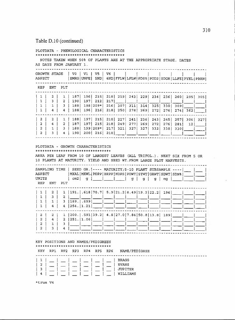
310
PLOTDATA - PHENOLOGICAL CHARACTERISTICS
Table D.IO (continued)
NOTES TAKEN WHEN 50% OF PLANTS ARE AT THE APPROPRIATE STAGE. DATES AS DAYS FROM JANUARY 1 .
GROWTH STAGE 11 VO 1 VI 1 V5 1 V6 1 1 1 1 1 1 1 1 1ASPECT 1EMRG1UNFE1 5NDl 6ND1FFLW1LFLW1PDO 51P0D21SDGR1LLFE|PYEL j PBRN|
REP ENT PLT
1 3. 1 3 1 1 11 1871 1961 2151 218 1 219| 243 1 2291 2341 236 1 2601 2951 30511 1 1 3 I 2 1I 1901 197 I 212 1 2171 1 1 1 1 1 1 11 1 1 1 1 3 1I 188| 1981 209^1 2161 3071 3111 3141 325| 3301 3091 1 11 3 I 4 1 4 11 188| 196 1 216 I 218| 2501 278 1 269| 272 1 276 1 274 1 3621 1
1 2 1 3 1 1 1i 188| 197 1 215 1 2181 227 1 24l| 2361 243 1 2451 2571 306 1 32711 2 1 4 1 2 1I 1871 197| 215 1 218 1 249 1 2771 269| 272 I 276 1 2 8 l l 12 1 11 3 1 1 I 3 11 1881 199| 209+ 1 217| 3211 3271 3271 332 1 338| 330| 1 11 2 1 3 I 4 11 1901 200| 216 1 218| 1 1 1 1 1 1 1 1
PLOTDATA - GROWTH CHARACTERISTICS * * * * * * * * * * * * * * * * * * * * * * * * * * * * * * * * *AREA PER LEAF FROM 10 OF LARGEST LEAVES (ALL T R IF O L .). NEXT SIX FROM 5 OR 10 PLANTS AT MATURITY. YIELD AND SEED WT.FROM LARGE PLOT HARVESTS.
SAMPLING TIME | SEED G R .|------- MATURITY;5 -1 0 PLANT SUBSAMPLE -------- |ASPECT IMXAL|MXWL|PDPP|BRPP|NDPS|PDWT|STWT|GRWT|SDWT|SDN%|UNITS I cm 21 g |_____ |______| | g | g | g | mg |______ |
REP ENT PLT
1 |191.I .618| 70 .7| 5 .9 | 2 1 .2 | 8 .4 9 | 1 9 .2 | 2 2 .2 | 1 9 6 12 I I 1 I I I I I I I3 |189. 1 .6 9 9 1 _____1_____ 1______1______1______1______1_____I4 1254.11.211___ I____I____I____I____I_I I
1 1200.1.591139.21 4 . 8 | 27.017.84150.8113.8| 18912 1251.11.061 I I I I 1___ 1____L3 I____I____I____I____ I____I____I____1____1____1.4 I____I____I____I____ I____I____I____I____I____1.
KEY POSITIONS AND NAMES/PEDIGREES * * * * * * * * * * * * * * * * * * * * * * * * * * * * * * * * *
KEY RPl RP2 RP3 RP4 RP5 RP6 NAME/PEDIGREE
BRAGG2 | _ l _ l _ l _ l _ l _ l EVANS3 1 __ 1 1 1 1 1 1 JUPITER4 I __ I I I I 1 I WILLIAMS
♦ t r u e V4
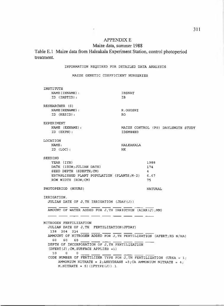
311
APPENDIX E Maize data, summer 1988
Table E.l Maize data from Haleakala Experiment Station, control photoperiod treatment.
INFORMATION REQUIRED FOR DETAILED DATA ANALYSIS
MAIZE GENETIC COEFFICIENT NURSERIES
INSTITUTENAME(INNAME): ID (IN S T ID ):
IBSNATIB
RESEARCHER (S)NAME(RENAME): ID (R E SID ):
R . OGOSHI RO
EXPERIMENTNAME (EXNAME): ID (EXPN):
MAIZE CONTROL (PO) DAYLENGTH STUDY IDSM88H0
LOCATIONNAME:ID (LO C ):
HALEAKALAHK
SEEDINGYEAR (lYR) 1988DATE (ISOW;JULIAN DATE) 174SEED DEPTH (SDEPTH;CM) 4ESTABLISHED PLANT POPULATION (PLANTS;M-2) 6 .6 7 ROW WIDTH (ROW;CM) 75
PHOTOPERIOD (HOURS) NATURAL
IRRIGATION.JULIAN DATE OF J,TH IRRIGATION (JD AY(J))
AMOUNT OF WATER ADDED FOR J,TH IRRIGTION (AIRR(J);M M )
NITROGEN FERTILIZATIONJULIAN DATE OF J,TH FERTILIZATION(JFDAY)
138 204 234AMMOUNT OF NITROGEN ADDED FOR J,TH FERTILIZATION (AFERT;KG N/HA)
60 60 60 ______________________________________________DEPTH OF INCORPORATION OF J,TH FERTILIZATION (D FE R T(J); CM,SURFACE APPLIED =1)10 0 0
CODE NUMBER OF FERTILIZER TYPE FOR J,TH FERTILIZATION (UREA = 1;AMMONIUM NITRATE = 2;ANHYDRANE =3;CA AMMONIUM NITRATE = 4;M.NITRATE = 5)(IFTYPE(J)) 1
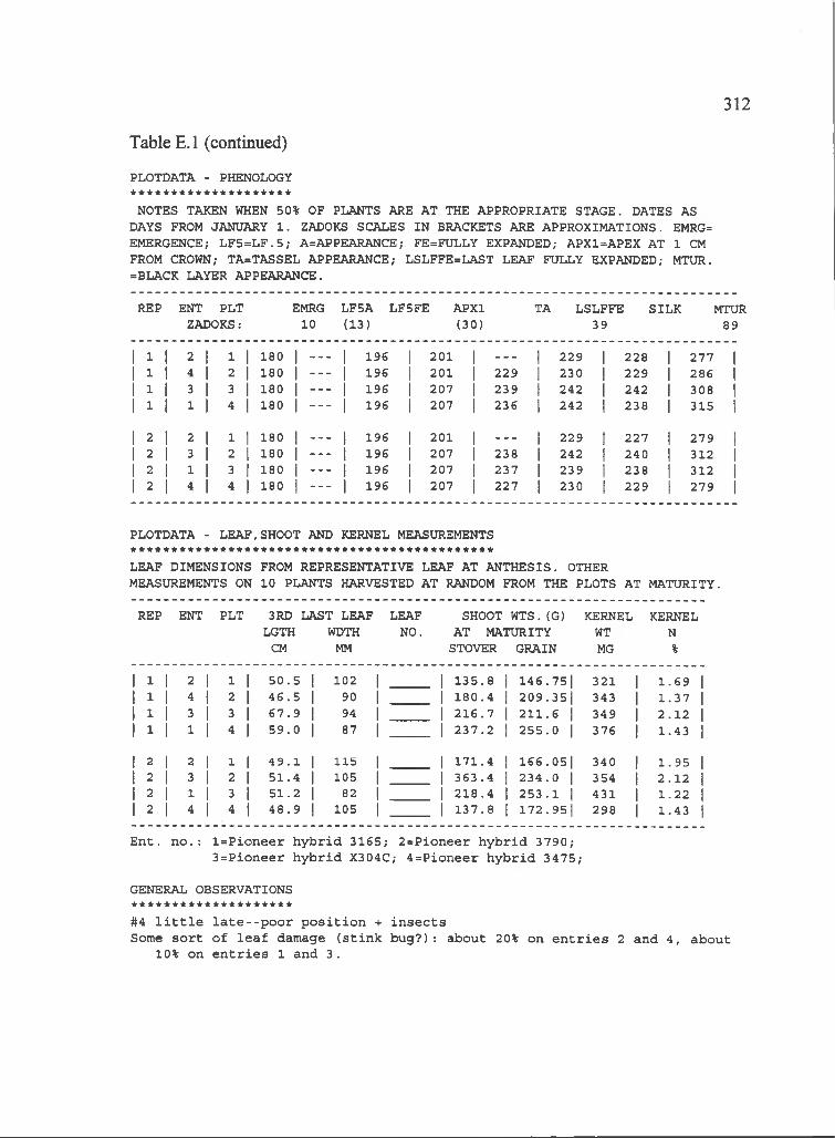
312
Table E.l (continued)
PLOTDATA - PHENOLOGY ********************
NOTES TAKEN WHEN 50% OF PLANTS ARE AT THE APPROPRIATE STAGE. DATES AS DAYS FROM JANUARY 1 . ZADOKS SCALES IN BRACKETS ARE APPROXIMATIONS. EMRG= EMERGENCE; L F5=LF .5 ; A=APPEARANCE; FE=FULLY EXPANDED; APX1=APEX AT 1 CM FROM CROWN; TA=TASSEL APPEARANCE; LSLFFE=LAST LEAF FULLY EXPANDED; MTUR. =BLACK LAYER APPEARANCE.
REP ENT PLT ZADOKS:
EMRG LF5A LF5FE APXl 10 (13) (30)
TA LSLFFE39
SILK MTUR89
1 1 2 1 1 180 ___ 1 196 201 ___ 229 228 2771 1 4 I 2 180 -----1 196 201 229 230 229 2861 1 3 I 3 180 -----1 196 207 239 242 242 3081 1 1 1 4 180 -----1 196 207 236 242 238 315
2 1 2 1 1 180 ___ j 196 201 ___ 229 227 2792 I 3 1 2 180 -----I 196 207 238 242 240 3122 I 1 I 3 180 -----I 196 207 237 239 238 3122 I 4 I 4 180 -----1 196 207 227 230 229 279
PLOTDATA - LEAF,SHOOT AND KERNEL MEASUREMENTS
LEAF DIMENSIONS FROM REPRESENTATIVE LEAF AT ANTHESIS. OTHER MEASUREMENTS ON 10 PLANTS HARVESTED AT RANDOM FROM THE PLOTS AT MATURITY.
REP ENT PLT 3RD LAST LEAF LGTH WDTH
CM MM
LEAFNO.
SHOOT WTS.(G) AT MATURITY
STOVER GRAIN
KERNELWTMG
KERNELN%
1 I 3 1 1 1 5 0 .5 1 102 1 1 1 3 5 .8 146 .751 321 1 1 .6 91 1 4 1 2 1 4 6 .5 90 I 1 8 0 .4 2 0 9 .35| 343 I 1 .3 71 I 3 1 3 6 7 .9 94 1 2 1 6 .7 2 1 1 .6 I 349 I 2 .1 21 1 1 I 4 I 5 9 .0 1 87 I 1 2 3 7 .2 2 5 5 .0 I 376 I 1 .4 3
2 1 2 1 1 1 4 9 .1 1 115 1 1 1 7 1 .4 1 6 6 .05| 340 1 1 .9 52 I 3 I 2 I 5 1 .4 105 1 3 6 3 .4 2 3 4 .0 I 354 I 2 .1 23 1 1 3 5 1 .2 82 1 2 1 8 .4 2 5 3 .1 1 431 I 1 .2 22 I 4 I 4 I 4 8 .9 1 105 1 I 1 3 7 .8 172 .951 298 1 .4 3
E n t. n o . : l= P io n e e r h y b r id 3 1 6 5 ; 2 = P io n e e r h y b r id 3 7 9 0 ;3 = P io n e e r h y b r id X304C; 4 = P io n e e r h y b r id 3 4 7 5 ;
GENERAL OBSERVATIONS * * * * * * * * * * * * * * * * * * * *
#4 l i t t l e l a t e - - p o o r p o s i t i o n + i n s e c t sSome s o r t o f l e a f damage (s t in )c b u g ? ) : a b ou t 20% on e n t r i e s 2 and 4 , a b ou t
10% on e n t r i e s 1 and 3 .
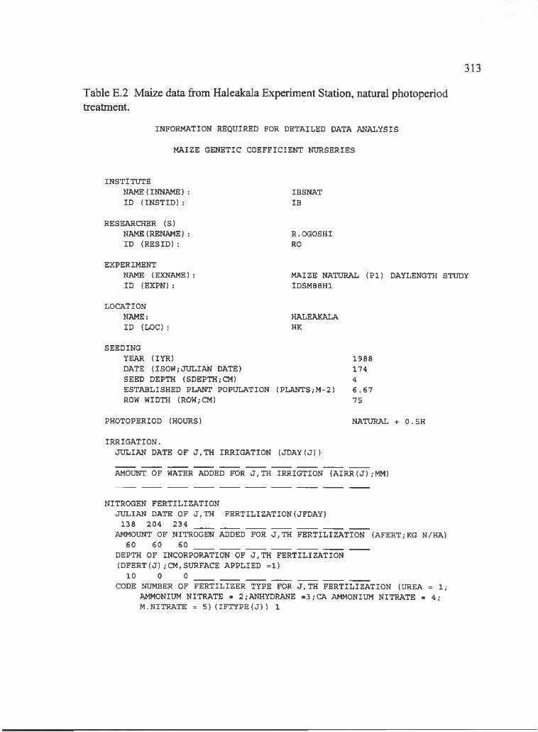
313
INFORMATION REQUIRED FOR DETAILED DATA ANALYSIS
MAIZE GENETIC COEFFICIENT NURSERIES
Table E.2 Maize data from Haleakala Experiment Station, natural photoperiodtreatment.
INSTITUTENAME(INNAME): ID (IN S T ID ):
IBSNATIB
RESEARCHER (S)NAME(RENAME): ID (R E SID ):
R.OGOSHI RO
EXPERIMENTNAME (EXNAME): ID (EXPN):
MAIZE NATURAL (P I) DAYLENGTH STUDY IDSM88H1
LOCATIONNAME:ID (LOO :
HALEAKALAHK
SEEDINGYEAR (lYR ) 1988DATE (ISOW;JULIAN DATE) 174SEED DEPTH (SDEPTH;CM) 4ESTABLISHED PLANT POPULATION ( PLANTS;M-2) 6 .6 7ROW WIDTH (ROW;CM) 75
PHOTOPERIOD (HOURS) NATURAL + 0.5H
IRRIGATION.JULIAN DATE OF J,TH IRRIGATION (JD AY(J))
AMOUNT OF WATER ADDED FOR J,TH IRRIGTION (AIRR(J);M M )
NITROGEN FERTILIZATIONJULIAN DATE OF J,TH FERTILIZATION(JFDAY)
138 204 234AMMOUNT OF NITROGEN ADDED FOR J,TH FERTILIZATION (AFERT;KG N/HA)
60 60 60 ______________________________________________DEPTH OF INCORPORATION OF J,TH FERTILIZATION (D FE R T(J); CM,SURFACE APPLIED =1)10 0 0
CODE NUMBER OF FERTILIZER TYPE FOR J,TH FERTILIZATION (UREA = 1;AMMONIUM NITRATE = 2;ANHYDRANE =3;CA AMMONIUM NITRATE = 4;M.NITRATE = 5)(IFTYPE(J)) 1
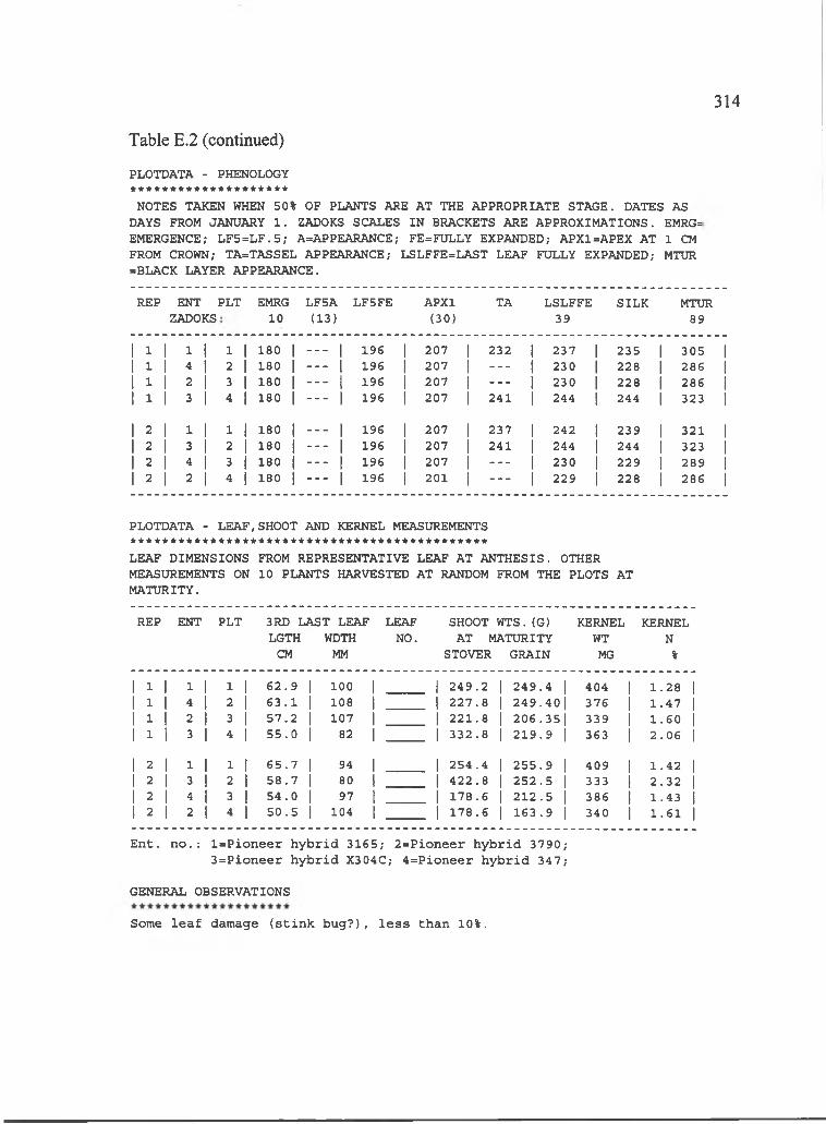
314
Table E.2 (continued)
PLOTDATA - PHENOLOGY * * * * * * * * * * * * * * * * * * * *
NOTES TAKEN WHEN 50% OF PLANTS ARE AT THE APPROPRIATE STAGE. DATES AS DAYS FROM JANUARY 1 . ZADOKS SCALES IN BRACKETS ARE APPROXIMATIONS. EMRG= EMERGENCE; L F5=L F .5 ; A=APPEARANCE; FE=FULLY EXPANDED; APX1=APEX AT 1 CM FROM CROWN; TA=TASSEL APPEARANCE; LSLFFE=LAST LEAF FULLY EXPANDED; MTUR =BLACK LAYER APPEARANCE.
REP ENTZADOKS
PLT EMRG10
LF5A(13)
LF5FE APXl(30)
TA LSLFFE39
SILK MTUR89
1 1 1 1 1 1 180 1 -----1 196 1 207 1 232 1 237 1 235 1 305 11 1 4 I 2 I 180 1 -----1 196 1 207 I ----- 1 230 I 228 I 286 Ij 1 2 1 3 I 180 I -----1 196 I 207 I ----- I 230 I 228 1 286 11 1 3 1 4 1 180 I -----1 196 I 207 I 241 1 244 1 244 1 323 1
1 2 1 1 1 1 180 1 ___ 1 196 1 207 1 237 1 242 1 239 1 321 11 3 3 1 2 1 180 I -----1 196 I 207 I 241 1 244 j 244 j 323 I1 2 4 I 3 I 180 I -----1 196 I 207 I ----- 1 230 I 229 1 289 11 2 2 I 4 I 180 1 -----1 196 I 201 I ----- 1 229 1 228 I 286 I
PLOTDATA - LEAF,SHOOT AND KERNEL MEASUREMENTS
LEAF DIMENSIONS FROM REPRESENTATIVE LEAF AT ANTHESIS. OTHER MEASUREMENTS ON 10 PLANTS HARVESTED AT RANDOM FROM THE PLOTS AT MATURITY.
REP ENT PLT 3RD LAST LEAF LGTH WDTH
CM MM
LEAFNO.
SHOOT WTS.(G) AT MATURITY
STOVER GRAIN
KERNELWTMG
KERNELN%
1 1 1 1 1 1 1 6 2 .9 1 100 1 1 2 4 9 .2 1 2 4 9 .4 1 404 1 1 .2 8 11 1 1 4 1 2 1 6 3 .1 I 108 I 1 2 2 7 .8 1 2 4 9 .40| 376 I 1 .4 7 I1 1 1 2 1 3 I 5 7 .2 I 107 1 1 2 2 1 .8 1 2 0 6 .35| 339 I 1 .6 0 I1 1 1 3 1 4 1 5 5 .0 I 82 I 1 3 3 2 .8 1 2 1 9 .9 1 363 I 2 .0 6 1
1 2 1 1 1 1 I 6 5 .7 1 94 1 1 2 5 4 .4 1 2 5 5 .9 1 409 1 1 .4 2 11 2 1 3 1 2 1 5 8 .7 1 80 1 1 4 2 2 .8 1 2 5 2 .5 1 333 1 2 .3 2 11 2 1 4 1 3 I 54 .0 I 97 1 1 1 7 8 .6 1 2 1 2 .5 1 386 1 1 .4 3 11 2 1 2 1 4 1 5 0 .5 1 104 I 1 1 7 8 .6 1 1 6 3 .9 1 340 I 1 .6 1 I
E n t. n o . : l= P io n e e r h y b r id 3 1 6 5 ; 2 = P io n e e r h y b r id 3 7 9 0 ;3 = P io n e e r h y b r id X304C; 4 = P io n e e r h y b r id 3 47 ;
GENERAL OBSERVATIONS
Some l e a f damage ( s t in k b u g ? ) , l e s s than 10%.

315
INFORMATION REQUIRED FOR DETAILED DATA ANALYSIS
MAIZE GENETIC COEFFICIENT NURSERIES
Table E.3 Maize data from Haleakala Experiment Station, 14 h photoperiodtreatment.
INSTITUTENAME( INNAME) : IBSNATID (IN S T ID ): IB
RESEARCHER (S)NAME(RENAME) : R . OGOSHIID (R E SID ): RO
EXPERIMENTNAME (EXNAME): MAIZE 14H (P2) DAYLENGTH STUDYID (EXPN): IDSM88H2
LOCATIONNAME: HALEAKALAID (L O C ): HK
SEEDINGYEAR (lYR ) 1988DATE (ISOW;JULIAN DATE) 174SEED DEPTH (SDEPTH;CM) 4ESTABLISHED PLANT POPULATION (PLANTS;M-2) 6 .6 7ROW WIDTH (ROW;CM) 75
PHOTOPERIOD (HOURS) 14
IRRIGATION.JULIAN DATE OF J,TH IRRIGATION (JD AY(J))
AMOUNT OF WATER ADDED FOR J,TH IRRIGTION (AIRR(J);M M )
NITROGEN FERTILIZATIONJULIAN DATE OF J,TH FERTILIZATION(JFDAY)
138 204 234AMMOUNT OF NITROGEN ADDED FOR J,TH FERTILIZATION (AFERT;KG N/HA)
60 60 60 ______________________________________________DEPTH OF INCORPORATION OF J,TH FERTILIZATION (D FE R T(J); CM,SURFACE APPLIED =1)10 0 0
CODE NUMBER OF FERTILIZER TYPE FOR J,TH FERTILIZATION (UREA = 1;AMMONIUM NITRATE = 2;ANHYDRANE =3;CA AMMONIUM NITRATE = 4;M.NITRATE = 5)(IFTYPE(J)) 1
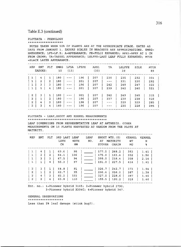
316
Table E.3 (continued)
PLOTDATA - PHENOLOGY * * * * * * * * * * * * * * * * * * * *
NOTES TAKEN WHEN 50% OF PLANTS ARE AT THE APPROPRIATE STAGE. DATES AS DAYS FROM JANUARY 1 . ZADOKS SCALES IN BRACKETS ARE APPROXIMATIONS. EMRG= EMERGENCE; L F5=LF .5 ; A=APPEARANCE; FE=FULLY EXPANDED; APX1=APEX AT 1 CM FROM CROWN; TA=TASSEL APPEARANCE; LSLFFE=LAST LEAF FULLY EXPANDED; MTUR =BLACK LAYER APPEARANCE.
REP ENT ZADOKS1
PLT EMRG10
LF5A(13)
LF5FE APXl(30)
TA LSLFFE39
SILK MTUR89
1 1 1 4 1 1 1 180 1 ___ 1 196 1 207 1 230 1 235 1 232 1 301 11 1 1 2 I 2 1 180 I -----1 201 I 207 I ----- 1 231 1 230 I 292 jI 1 1 3 I 3 I 180 I -----I 196 I 207 I 242 1 249 I 247 I 3221 1 1 3 I 4 1 180 I -----1 201 I 207 I 239 1 242 I 240 1 321 1
1 2 1 3 1 1 1 180 1 -----1 201 1 207 1 242 1 249 1 245 1 335 11 2 1 3 1 2 1 180 1 -----1 196 1 207 I 237 1 239 1 238 1 3101 2 1 4 I 3 1 180 I -----1 196 1 207 1 ----- 1 229 I 229 I 285 11 2 1 2 I 4 1 180 1 -----1 196 1 207 1 ----- 1 230 I 228 I 285 I
PLOTDATA - LEAF,SHOOT AND KERNEL MEASUREMENTS
LEAF DIMENSIONS FROM REPRESENTATIVE LEAF AT ANTHESIS. OTHER MEASUREMENTS ON 10 PLANTS HARVESTED AT RANDOM FROM THE PLOTS AT MATURITY.
REP ENT PLT 3RD LAST LGTH
CM
LEAFWDTH
MM
LEAFNO.
SHOOT WTS.(G) AT MATURITY
STOVER GRAIN
KERNELWTMG
KERNELN%
1 3 1 4 1 1 1 6 9 .6 1 98 1 1 7 7 .5 1 2 6 8 .2 353 i 1 .4 1 11 3 I 2 1 2 1 6 4 .1 I 106 1 1 7 5 .0 I 1 8 3 .4 352 1 1 .5 6 I1 3 1 3 1 3 1 6 7 .5 1 94 I 3 9 9 .0 1 2 1 8 .4 358 1 2 .1 4 I1 3 1 1 1 4 1 5 5 .3 1 97 I 1 9 1 .0 I 2 2 7 .5 414 1 1 .4 1 1
1 2 1 3 1 1 1 6 4 .8 1 93 1 3 2 6 .7 1 2 4 2 .7 373 1 1 .9 4 1I 2 I 1 I 2 1 6 2 .7 I 95 I 2 9 6 .6 1 2 5 8 .2 387 I 1 .3 8 I1 2 1 4 1 3 1 6 5 .2 1 103 1 2 2 7 .0 1 2 2 8 .6 387 I 1 .4 6 1I 2 I 2 1 4 1 6 3 .8 I 110 I 1 5 5 .5 I 1 9 2 .2 318 I 1 .4 6 1
E n t. n o . : l= P io n e e r h y b r id 31S 5 ; 2 = P io n e e r h y b r id 3790 ;3 = P io n e e r h y b r id X304C; 4 = P io n e e r h y b r id 347 .
GENERAL OBSERVATIONS * * * * * * * * * * * * * * * * * * * *L e ss th an 5% l e a f damage ( s t in k bu g?)
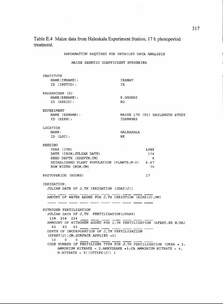
317
INFORMATION REQUIRED FOR DETAILED DATA ANALYSIS
MAIZE GENETIC COEFFICIENT NURSERIES
Table E.4 Maize data from Haleakala Experiment Station, 17 h photoperiodtreatment.
INSTITUTENAME( INNAME) : IBSNATID (IN S T ID ): IB
RESEARCHER (S)NAME(RENAME) : R . OGOSHIID (R E SID ): RO
EXPERIMENTNAME (EXNAME): MAIZE 17H (P3) DAYLENGTH STUDYID (EXPN): IDSM88H3
LOCATIONNAME: HALEAKALAID (LOO : HK
SEEDINGYEAR (lYR) 1988DATE (ISOW,-JULIAN DATE) 174SEED DEPTH (SDEPTH,-CM) 4ESTABLISHED PLANT POPULATION (PLANTS,-M -2) 6 .6 7ROW WIDTH (ROW;CM) 75
PHOTOPERIOD (HOURS) 17
IRRIGATION.JXmiAN DATE OF J,TH IRRIGATION (JD AY (J))
AMOUNT OF WATER ADDED FOR J,TH IRRIGTION (AIRR(J),-MM)
NITROGEN FERTILIZATIONJULIAN DATE OF J,TH FERTILIZATION(JFDAY)
138 204 234AMMOUNT OF NITROGEN ADDED FOR J,TH FERTILIZATION (AFERT,-KG N/HA)
60 60 60 ______________________________________________DEPTH OF INCORPORATION OF J,TH FERTILIZATION (D FE R T(J); CM,SURFACE APPLIED =1)10 0 0
CODE NUMBER OF FERTILIZER TYPE FOR J,TH FERTILIZATION (UREA = 1;AMMONIUM NITRATE = 2,-ANHYDRANE =3;CA AMMONIUM NITRATE = 4;M.NITRATE = 5)(IFTYPE(J)) 1
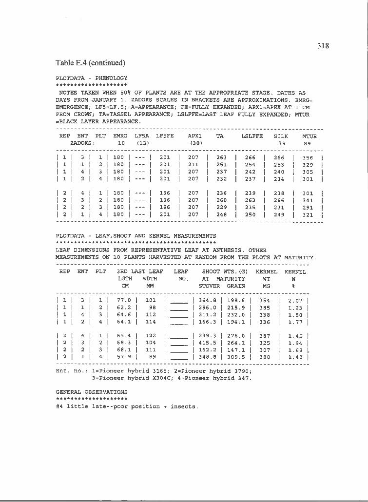
318
Table E.4 (continued)
PLOTDATA - PHENOLOGY ********************
NOTES TAKEN WHEN 50% OF PLANTS ARE AT THE APPROPRIATE STAGE. DATES AS DAYS FROM JANUARY 1 . ZADOKS SCALES IN BRACKETS ARE APPROXIMATIONS. EMRG= EMERGENCE; L F5=LF .5 ; A=APPEARANCE; FE=FULLY EXPANDED; APX1=APEX AT 1 CM FROM CROWN; TA=TASSEL APPEARANCE; LSLFFE=LAST LEAF FULLY EXPANDED; MTUR =BLACK LAYER APPEARANCE.
REP ENTZADOKS:
PLT EMRG10
LF5A(13)
LF5FE APXl(30)
TA LSLFFE SILK39
MTUR89
1 1 1 2 1 1 1 180 1 ___ 1 201 1 207 1 263 1 266 1 266 1 356 11 1 1 1 2 1 180 1 -----1 201 I 211 I 251 1 254 1 253 1 329 11 1 1 4 I 3 1 180 1 -----1 201 I 207 I 237 1 242 I 240 1 305 I1 1 1 2 j 4 1 180 I -----1 201 I 207 I 232 1 237 I 234 j 301 1
1 2 1 4 1 1 1 180 1 ___ 1 196 1 207 1 236 1 239 1 238 1 301 11 2 1 2 I 2 1 180 1 -----1 196 I 207 I 260 1 263 I 266 I 341 11 2 1 2 I 3 1 180 1 - - - 1 196 1 207 I 229 1 235 I 231 I 2911 2 1 1 1 4 1 180 1 -----1 201 I 207 I 248 1 250 I 249 1 321 I
PLOTDATA - LEAF,SHOOT AND KERNEL MEASUREMENTS
LEAF DIMENSIONS FROM REPRESENTATIVE LEAF AT ANTHESIS. OTHER MEASUREMENTS ON 10 PLANTS HARVESTED AT RANDOM FROM THE PLOTS AT MATURITY.
REP ENT PLT 3RD LAST LEAF LGTH WDTH
CM MM
LEAFNO.
SHOOT WTS.(G) AT MATURITY
STOVER GRAIN
KERNELWTMG
KERNELN%
1 1 1 3 1 1 1 7 7 .0 1 101 1 3 6 4 .8 1 9 8 .6 1 354 1 2 .0 7 11 1 1 1 1 2 1 6 2 .2 1 98 I 2 9 6 .0 2 1 5 .9 I 385 I 1 .2 3 I1 1 4 1 3 1 64 .6 I 112 I 2 1 1 .2 2 3 2 .0 I 338 I 1 .5 0 I1 1 1 2 1 4 1 6 4 .1 I 114 I 1 6 6 .3 1 9 4 .1 I 336 I 1 .7 7 I
1 2 1 4 1 1 1 65 .4 1 122 1 2 3 9 .3 2 7 6 .0 1 387 1 1 .4 5 11 2 1 3 1 2 1 6 8 .3 1 104 I 4 1 5 .5 2 6 4 .1 1 325 1 1 .9 4 I1 2 1 2 1 3 I 6 8 .1 I 111 I 1 6 2 .2 1 4 7 .1 1 307 1 1 .6 9 11 2 1 1 1 4 1 5 7 .9 1 89 I 3 4 8 .8 3 0 9 .5 I 380 1 1 .4 0 1
E n t. n o . : l= P io n e e r h y b r id 3 1 6 5 ; 2 = P io n e e r h y b r id 3 7 9 0 ;3 = P io n e e r h y b r id X304C; 4 = P io n e e r h y b r id 3 4 7 .
GENERAL OBSERVATIONS * * * * * * * * * * * * * * * * * * * *#4 l i t t l e l a t e - - p o o r p o s i t i o n + i n s e c t s .
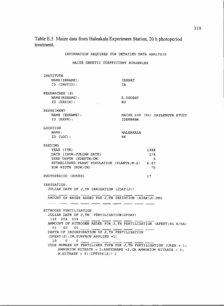
319
INFORMATION REQUIRED FOR DETAILED DATA ANALYSIS
MAIZE GENETIC COEFFICIENT NURSERIES
Table E.5 Maize data from Haleakala Experiment Station, 20 h photoperiodtreatment.
INSTITUTENAME(INNAME): IBSNATID (IN S T ID ): IB
RESEARCHER (S)NAME(RENAME) : R . OGOSHIID (R E SID ): RO
EXPERIMENTNAME (EXNAME): MAIZE 20H (P4) DAYLENGTH STUDYID (EXPN): IDSM88H4
LOCATIONNAME: HALEAKALAID (LO C ): HK
SEEDINGYEAR (lYR ) 1988DATE (ISOW;JULIAN DATE) 174SEED DEPTH (SDEPTH;CM) 4ESTABLISHED PLANT POPULATION (PLANTS;M-2) 6 .6 7 ROW WIDTH (ROW;CM) 75
PHOTOPERIOD (HOURS) 17
IRRIGATION.JULIAN DATE OF J,TH IRRIGATION (JD AY (J))
AMOUNT OF WATER ADDED FOR J,TH IRRIGTION (AIRR(J);M M )
NITROGEN FERTILIZATIONJULIAN DATE OF J,TH FERTILIZATION(JFDAY)
138 204 234AMMOUNT OF NITROGEN ADDED FOR J,TH FERTILIZATION (AFERT;KG N/HA)
60 60 60 ______________________________________________DEPTH OF INCORPORATION OF J,TH FERTILIZATION (D FE R T(J); CM,SURFACE APPLIED =1)10 0 0
CODE NUMBER OF FERTILIZER TYPE FOR J,TH FERTILIZATION (UREA = 1;AMMONIUM NITRATE = 2;ANHYDRANE =3;CA AMMONIUM NITRATE = 4;M.NITRATE = 5)(IFTYPE(J)) 1
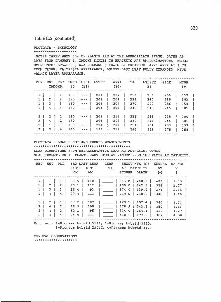
320
Table E.5 (continued)
PLOTDATA - PHENOLOGY * * * * * * * * * * * * * * * * * * * *
NOTES TAKEN WHEN 50% OF PLANTS ARE AT THE APPROPRIATE STAGE. DATES AS DAYS FROM JANUARY 1 . ZADOKS SCALES IN BRACKETS ARE APPROXIMATIONS. EMRG= EMERGENCE; L F5=LF .5 ; A=APPEARANCE; FE=FULLY EXPANDED; APX1=APEX AT 1 CM FROM CROWN; TA=TASSEL APPEARANCE; LSLFFE=LAST LEAF FULLY EXPANDED; MTUR =BLACK LAYER APPEARANCE.
REP ENT PLT ZADOKS:
EMRG10
LF5A(13)
LF5FE APXl(30)
TA LSLFFE39
SILK MTUR89
I 3 1 1 1 1 1 180 1 ___ 1 201 1 207 253 1 256 256 i 337 11 3 1 2 1 3 1 180 I -----1 201 1 207 236 I 240 239 1 303 I1 3 1 3 I 3 I 180 I -----1 201 I 207 270 I 272 286 1 359 11 3 1 4 I 4 1 180 I -----1 201 I 207 242 1 246 246 1 305 I
1 2 1 2 1 1 1 180 1 ___ 1 201 1 211 235 1 238 238 1 300 11 2 1 4 j 2 I 180 I -----1 201 1 207 239 I 244 244 1 305 11 2 1 1 1 3 1 180 I -----1 201 1 207 251 1 254 253 1 337 I1 3 1 3 1 4 1 180 I -----1 196 1 211 266 I 269 275 1 358 1
PLOTDATA - LEAF,SHOOT AND KERNEL MEASUREMENTS
LEAF DIMENSIONS FROM REPRESENTATIVE LEAF AT ANTHESIS. OTHER MEASUREMENTS ON 10 PLANTS HARVESTED AT RANDOM FROM THE PLOTS AT MATURITY.
REP ENT PLT 3RD LAST LEAF LGTH WDTH
CM MM
LEAFNO.
SHOOT WTS.(G) AT MATURITY
STOVER GRAIN
KERNELWTMG
KERNELN%
1 3 1 1 1 1 1 6 6 .5 1 110 1 3 1 5 .8 2 6 8 .8 1 403 1 1 .3 5 11 3 1 3 1 3 1 7 0 .1 1 112 I 1 6 6 .0 1 4 2 .5 I 356 I 1 .7 7 11 3 I 3 I 3 1 6 5 .4 1 93 I 5 7 4 .0 1 3 9 .0 I 374 I 2 .8 5 11 3 I 4 1 4 1 7 7 .4 I 333 1 2 3 9 .0 2 1 8 .5 1 340 I 1 .4 6 1
1 3 1 3 1 1 1 6 7 .2 1 107 1 1 2 9 .5 1 5 2 .4 1 340 1 1 .6 4 11 3 I 4 1 3 1 6 5 .9 1 105 I 2 7 8 .9 2 4 3 .5 1 350 1 1 .5 31 3 1 1 1 3 1 6 2 .1 1 95 1 3 3 4 .0 2 6 4 .4 I 410 1 1 .2 7 I1 3 1 3 I 4 1 7 4 .9 I 311 1 4 1 0 .2 1 7 7 .6 I 362 1 4 .58 I
E n t. n o . : l= P io n e e r h y b r id 3 1 6 5 ; 2 = P io n e e r h y b r id 3 7 9 0 ;3 = P io n e e r h y b r id X304C; 4 = P io n e e r h y b r id 3 4 7 .
GENERAL OBSERVATIONS * * * * * * * * * * * * * * * * * * * *

321
INFORMATION REQUIRED FOR DETAILED DATA ANALYSIS
MAIZE GENETIC COEFFICIENT NURSERIES
Table E.6 Maize data from Kuiaha Experiment Site, control photoperiod treatment.
INSTITUTENAME(INNAME): ID (IN S T ID ):
IBSNATIB
RESEARCHER (S)NAME(RENAME): ID (R E SID ):
R.OGOSHI RO
EXPERIMENTNAME (EXNAME): ID (EXPN):
MAIZE CONTROL (PO) DAYLENGTH STUDY IDSM88K0
LOCATIONNAME:ID (LO C ):
KUIAHAKU
SEEDINGYEAR (lYR) 1988DATE (ISOW,-JULIAN DATE) 174SEED DEPTH (SDEPTH,-CM) 4ESTABLISHED PLANT POPULATION (PLANTS,-M -2) 6 .6 7ROW WIDTH (ROW;CM) 75
PHOTOPERIOD (HOURS) NATURAL
IRRIGATION.JULIAN DATE OF J,TH IRRIGATION (JD AY (J))
AMOUNT OF WATER ADDED FOR J,TH IRRIGTION (AIRR(J);M M )
NITROGEN FERTILIZATIONJULIAN DATE OF J,TH FERTILIZATION(JFDAY)
138 204 234AMMOUNT OF NITROGEN ADDED FOR J,TH FERTILIZATION (AFERT,-KG N/HA)
60 60 60 ______________________________________________DEPTH OF INCORPORATION OF J,TH FERTILIZATION (DFERT (J ) ,-CM, SURFACE APPLIED =1)10 0 0
CODE NUMBER OF FERTILIZER TYPE FOR J,TH FERTILIZATION (UREA = 1;AMMONIUM NITRATE = 2,-ANHYDRANE =3,-CA AMMONIUM NITRATE = 4 ,-M.NITRATE = 5)(IFTYPE(J)) 1

322
Table E.6 (continued)
PLOTDATA - PHENOLOGY ********************
NOTES TAKEN WHEN 50% OF PLANTS ARE AT THE APPROPRIATE STAGE. DATES AS DAYS FROM JANUARY 1 . ZADOKS SCALES IN BRACKETS ARE APPROXIMATIONS. EMRG= EMERGENCE; LF5=LF .5; A=APPEARANCE; FE=FULLY EXPANDED; APX1=APEX AT 1 CM FROM CROWN; TA=TASSEL APPEARANCE; LSLFFE=LAST LEAF FULLY EXPANDED; MTUR =BLACK LAYER APPEARANCE.
REP ENT ZADOKS;
PLT EMRG10
LF5A(13)
LF5FE APXl(30)
TA LSLFFE39
SILK MTUR89
1 1 1 3 1 1 1 180 1 ___ 1 194 1 201 1 232 1 335 1 236 1 296 11 1 1 1 1 3 1 180 I -----I 196 I 207 I 230 1 335 1 232 I 301 I1 1 1 2 I 3 1 180 I -----1 201 I 201 I ----- 223 I 280 I1 1 1 4 I 4 1 180 I -----1 201 I 207 I ----- 1 229 1 228 I 285 1
1 2 1 2 1 1 1 180 1 ___ 1 196 1 201 1 ___ 1 ___ 1 223 1 280 11 2 1 3 1 3 1 180 1 -----I 194 I 201 I 234 1 337 1 236 I 296 I1 2 1 4 1 3 1 180 1 -----1 196 I 201 I ----- I 229 j 228 I 286 I1 2 1 1 j 4 I 180 1 -----1 196 I 201 I 232 1 337 I 235 I 301 I
PLOTDATA - LEAF,SHOOT AND KERNEL MEASUREMENTS
LEAF DIMENSIONS FROM REPRESENTATIVE LEAF AT ANTHESIS. OTHER MEASUREMENTS ON 10 PLANTS HARVESTED AT RANDOM FROM THE PLOTS AT MATURITY.
REP ENT PLT 3RD LAST LEAF LGTH WDTH
CM MM
LEAFNO.
SHOOT WTS.(G) AT MATURITY
STOVER GRAIN
KERNELWTMG
KERNELN%
1 1 1 3 1 1 1 5 0 .7 1 98 1 1 3 1 9 .9 2 1 4 .45| 366 1 1 .9 9 11 1 1 1 I 3 1 4 9 .5 I 89 I 1 2 2 8 .7 2 7 6 .60| 401 I 1 .4 1 jI 1 I 3 1 3 I 4 7 .2 I 95 I 1 1 5 5 .0 1 3 7 .05| 323 I 1 .8 9 j1 1 1 4 I 4 1 5 2 .2 I 90 I 1 1 6 8 .7 2 1 0 .65| 357 I 1 .5 6 1
1 3 1 3 1 1 1 4 7 .0 1 104 1 1 1 7 9 .3 1 8 6 .85| 364 1 1 .6 5 11 3 I 3 I 3 1 54 .0 I 95 I I 2 4 9 .0 2 1 7 .35| 357 2 .1 4 I1 3 1 4 1 3 1 5 5 .9 I 100 I I 2 7 6 .0 2 3 8 .25| 333 I 1 .5 6 I1 3 1 1 1 4 1 6 3 .4 I 90 I 1 2 4 2 .0 2 5 6 .80| 422 I 1 .4 3 I
E n t. n o . : l= P io n e e r h y b r id 3 1 6 5 ; 2 = P io n e e r h y b r id 3 7 9 0 ;3 = P io n e e r h y b r id X304C; 4 = P io n e e r h y b r id 3 47 .
GENERAL OBSERVATIONS * * * * * * * * * * * * * * * * * * * *

323
INFORMATION REQUIRED FOR DETAILED DATA ANALYSIS
MAIZE GENETIC COEFFICIENT NURSERIES
Table E.7 Maize data from Kuiaha Experiment Site, natural photoperiod treatment.
INSTITUTENAME(INNAME): ID (IN S T ID ):
IBSNATIB
RESEARCHER (S)NAME(RENAME): ID (R E SID ):
R . OGOSHI RO
EXPERIMENTNAME (EXNAME): ID (EXPN):
MAIZE NATURAL (P I) DAYLENGTH STUDY IDSM88K1
LOCATIONNAME:ID (LO C ):
KUIAHAKU
SEEDINGYEAR (lYR) 1988DATE (ISOW;JULIAN DATE) 174SEED DEPTH (SDEPTH;CM) 4ESTABLISHED PLANT POPULATION (PLANTS;M-2) 6 .6 7 ROW WIDTH (ROW;CM) 75
PHOTOPERIOD (HOURS) NATURAL + 0.5H
IRRIGATION.JULIAN DATE OF J,TH IRRIGATION (JD AY(J))
AMOUNT OF WATER ADDED FOR J,TH IRRIGTION (AIRR(J);M M )
NITROGEN FERTILIZATIONJULIAN DATE OF J,TH FERTILIZATION(JFDAY)
138 204 234AMMOUNT OF NITROGEN ADDED FOR J,TH FERTILIZATION (AFERT;KG N/HA)
60 60 60 ______________________________________________DEPTH OF INCORPORATION OF J,TH FERTILIZATION (D FE R T(J); CM,SURFACE APPLIED =1)10 0 0
CODE NUMBER OF FERTILIZER TYPE FOR J,TH FERTILIZATION (UREA = 1;AMMONIUM NITRATE = 2;ANHYDRANE =3;CA AMMONIUM NITRATE = 4;M.NITRATE = 5)(IFTYPE(J)) 1
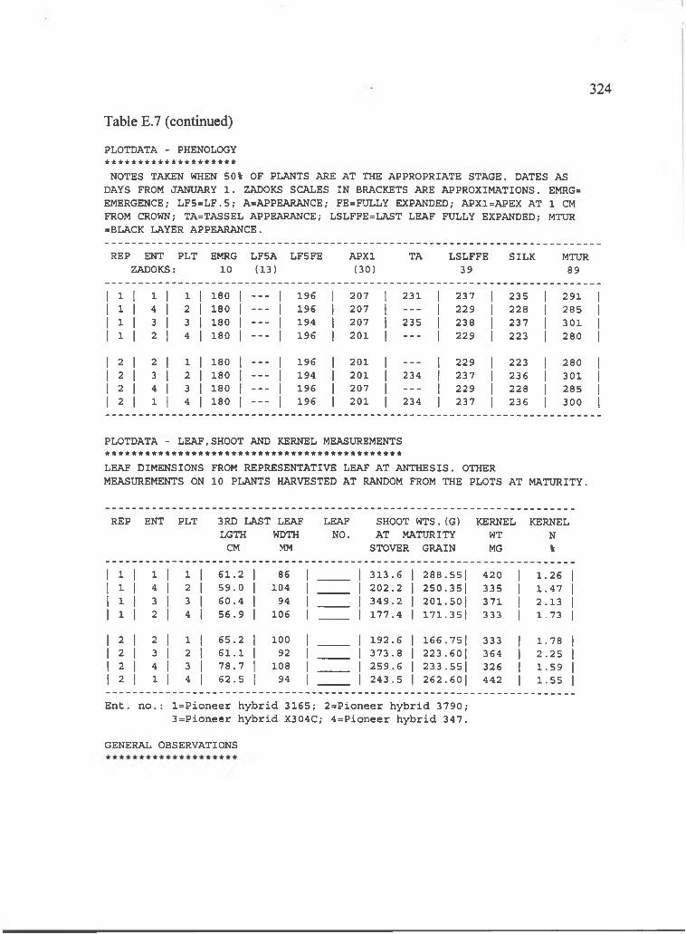
324
Table E.7 (continued)
PLOTDATA - PHENOLOGY ********************NOTES TAKEN WHEN 50% OF PLANTS ARE AT THE APPROPRIATE STAGE. DATES AS
DAYS FROM JANUARY 1 . ZADOKS SCALES IN BRACKETS ARE APPROXIMATIONS. EMRG= EMERGENCE; L F5=L F .5 ; A=APPEARANCE; FE=FULLY EXPANDED; APX1=APEX AT 1 CM FROM CROWN; TA=TASSEL APPEARANCE; LSLFFE=LAST LEAF FULLY EXPANDED; MTUR =BLACK LAYER APPEARANCE.
REP ENT ZADOKS:
PLT EMRG10
LF5A(13)
LF5FE APXl(30)
TA LSLFFE39
SILK MTUR89
1 1 1 1 1 1 1 180 1 ___ 1 196 1 207 1 231 1 237 1 235 1 291 11 1 1 4 I 2 1 180 I -----1 196 1 207 I ----- 1 229 1 228 I 285 11 1 1 3 1 3 I 180 1 -----1 194 I 207 I 235 1 238 I 237 I 301 11 1 1 2 1 4 1 180 I -----I 196 1 201 I ----- I 229 1 223 1 280 I
1 2 1 2 1 1 1 180 1 ___ 1 196 1 201 1 ___ 1 229 1 223 1 280 11 2 1 3 j 2 1 180 I -----1 194 I 201 I 234 1 237 I 236 I 301 II 2 1 4 1 3 1 180 1 -----1 196 I 207 I ----- I 229 I 228 I 285 I1 2 1 1 j 4 1 180 1 -----1 196 I 201 I 234 I 237 I 236 I 300 1
PLOTDATA - LEAF,SHOOT AND KERNEL MEASUREMENTS
LEAF DIMENSIONS FROM REPRESENTATIVE LEAF AT ANTHESIS. OTHER MEASUREMENTS ON 10 PLANTS HARVESTED AT RANDOM FROM THE PLOTS AT MATURITY.
REP ENT PLT 3RD LAST LEAF LGTH WDTH
CM MM
LEAFNO.
SHOOT WTS.(G) AT MATURITY
STOVER GRAIN
KERNELWTMG
KERNELN%
1 ^ 1 1 1 1 1 6 1 .2 1 86 1 313 .6 2 8 8 .55| 420 1 1 .2 6 11 1 t 4 1 2 1 5 9 .0 I 104 I 2 0 2 .2 2 5 0 .35| 335 1 .4 71 1 1 3 1 3 1 6 0 .4 I 94 I 3 4 9 .2 2 0 1 .50| 371 2 .1 31 1 1 2 1 4 1 5 6 .9 1 106 1 1 7 7 .4 171 .351 3 3 3 j 1 . 73 I
1 2 1 2 1 1 1 6 5 .2 1 100 1 1 9 2 .6 1 6 6 .75| 333 1 1 .7 8 11 2 1 3 1 2 1 6 1 .1 1 92 1 3 7 3 .8 2 2 3 .60| 364 I 2 .2 5 I1 2 1 4 1 3 1 7 8 .7 I 108 1 2 5 9 .6 2 3 3 .55| 326 I 1 .5 91 2 1 1 I 4 1 6 2 .5 1 94 1 243 .5 2 6 2 .60| 442 I 1 .5 5 1
E n t. n o . : l= P io n e e r h y b r id 3 1 6 5 ; 2 = P io n e e r h y b r id 3 7 9 0 ;3 = P io n e e r h y b r id X304C; 4 = P io n e e r h y b r id 3 47 .
GENERAL OBSERVATIONS

INFORMATION REQUIRED FOR DETAILED DATA ANALYSIS
MAIZE GENETIC COEFFICIENT NURSERIES
325
Table E.8 Maize data from Kuiaha Experiment Site, 14 h photoperiod treatment.
INSTITUTENAME( INNAME) : IBSNATID (IN S T ID ): IB
RESEARCHER (S)NAME(RENAME) : R . OGOSHIID (R E SID ): RO
EXPERIMENTNAME (EXNAME): MAIZE 14H (P2) DAYLENGTH STUDYID (EXPN): IDSM88K2
LOCATIONNAME: KUIAHAID (LO C ): KU
SEEDINGYEAR (lYR ) 1988DATE (ISOW,-JULIAN DATE) 174SEED DEPTH (SDEPTH,-CM) 4ESTABLISHED PLANT POPULATION (PLANTS,-M-2) 6 .6 7ROW WIDTH (ROW;CM) 75
PHOTOPERIOD (HOURS) 14
IRRIGATION.JULIAN DATE OF J,TH IRRIGATION (JD AY (J))
AMOUNT OF WATER ADDED FOR J,TH IRRIGTION (AIRR(J),-MM)
NITROGEN FERTILIZATIONJULIAN DATE OF J,TH FERTILIZATION(JFDAY)
138 204 234AMMOUNT OF NITROGEN ADDED FOR J,TH FERTILIZATION (AFERT,-KG N/HA)
60 60 60 ______________________________________________DEPTH OF INCORPORATION OF J,TH FERTILIZATION (D FE R T(J); CM,SURFACE APPLIED =1)10 0 0
CODE NUMBER OF FERTILIZER TYPE FOR J,TH FERTILIZATION (UREA = 1;AMMONIUM NITRATE = 2,-ANHYDRANE =3,-CA AMMONIUM NITRATE = 4 ,-M.NITRATE = 5)(IFTYPE(J)) 1
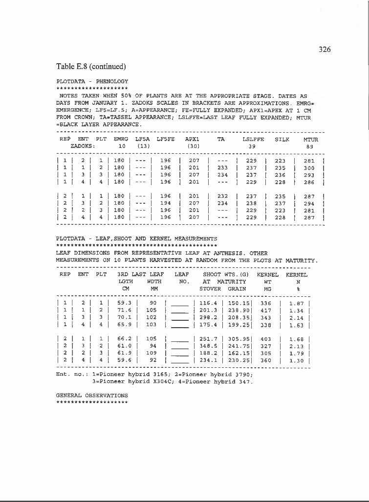
326
Table E.8 (continued)
PLOTDATA - PHENOLOGY ********************
NOTES TAKEN WHEN 50% OF PLANTS ARE AT THE APPROPRIATE STAGE. DATES AS DAYS FROM JANUARY 1 . ZADOKS SCALES IN BRACKETS ARE APPROXIMATIONS. EMRG= EMERGENCE; L F5=L F .5 ; A=APPEARANCE; FE=FULLY EXPANDED; APX1=APEX AT 1 CM FROM CROWN; TA=TASSEL APPEARANCE; LSLFFE=LAST LEAF FULLY EXPANDED; MTUR =BLACK LAYER APPEARANCE.
REP ENT ZADOKS:
PLT EMRG10
LF5A(13)
LF5FE APXl(30)
TA LSLFFE39
SILK MTUR89
1 3 1 2 1 1 1 180 1 ___ 1 196 207 ___ 1 229 1 223 1 281 11 3 I 1 I 2 1 180 1 ---- 1 196 201 233 1 237 I 235 1 300 1I 3 I 3 I 3 I 180 1 ---- 1 196 207 234 1 237 I 236 I 293 I1 3 1 4 I 4 I 180 j ---- 1 196 201 ----- 1 229 1 228 I 286 I
1 2 1 1 1 1 1 180 1 ---- 1 196 201 232 1 237 1 235 1 287 11 2 I 3 I 2 1 180 I . . . I 194 207 234 1 238 1 237 I 294 1I 2 I 2 1 3 1 180 I -----1 196 201 ----- 1 229 1 223 1 281 11 2 I 4 I 4 I 180 I -----1 196 207 ----- 1 229 I 228 I 287 I
PLOTDATA - LEAF,SHOOT AND KERNEL MEASUREMENTS
LEAF DIMENSIONS FROM REPRESENTATIVE LEAF AT ANTHESIS. OTHER MEASUREMENTS ON 10 PLANTS HARVESTED AT RANDOM FROM THE PLOTS AT MATURITY.
REP ENT PLT 3RD LAST T,EAF LGTH WDTH
CM MM
LEAFNO.
SHOOT WTS. (G) AT MATURITY
STOVER GRAIN
KERNELWTMG
KERNELN%
1 3 1 2 1 1 1 5 9 .3 1 90 1 1 1 6 .4 150 .151 336 1 1 .8 7 11 1 1 1 I 2 1 7 1 .6 I 105 j 2 0 1 .3 2 3 8 .90| 417 I 1 .3 4 I1 3 I 3 1 3 I 7 0 .1 I 102 I 2 9 8 .2 208.35,1 343 I 2 .1 4 II 1 I 4 I 4 1 6 5 .9 I 103 1 1 7 5 .4 1 9 9 .25| 338 I 1 .6 3 I
1 2 1 1 1 1 1 6 6 .2 1 105 1 2 5 1 .7 3 0 5 .95| 403 1 1 .6 8 11 2 1 3 I 2 1 6 1 .0 1 94 I 3 4 8 .5 241 .751 327 I 2 .1 3 11 2 1 2 1 3 1 6 1 .9 I 109 I 1 8 8 .2 1 6 2 .15| 305 I 1 .7 9 I1 2 1 4 1 4 I 5 9 .6 1 92 I 234 .1 2 3 0 .25| 360 I 1 .3 0 I
E n t. n o . : l= P io n e e r h y b r id 3 1 6 5 ; 2 = P io n e e r h y b r id 3 7 9 0 ;3 = P io n e e r h y b r id X304C; 4 = P io n e e r h y b r id 3 47 .
GENERAL OBSERVATIONSI t * * * * * * * * * * * * * * * * * * *

INFORMATION REQUIRED FOR DETAILED DATA ANALYSIS
MAIZE GENETIC COEFFICIENT NURSERIES
327
Table E.9 Maize data from Kuiaha Experiment Site, 17 h photoperiod treatment.
INSTITUTENAME( INNAME) : IBSNATID (IN S T ID ): IB
RESEARCHER (S)NAME(RENAME) : R . OGOSHIID (R E SID ): RO
EXPERIMENTNAME (EXNAME): MAIZE 17H (P3) DAYLENGTH STUDYID (EXPN): IDSM88K3
LOCATIONNAME: KUIAHAID (LO C ): KU
SEEDINGYEAR (lYR ) 1988DATE (ISOW;JULIAN DATE) 174SEED DEPTH (SDEPTH;CM) 4ESTABLISHED PLANT POPULATION (PLANTS;M-2) 6 .6 7 ROW WIDTH (ROW;CM) 75
PHOTOPERIOD (HOURS) 17
IRRIGATION.JULIAN DATE OF J,TH IRRIGATION (JD AY (J))
AMOUNT OF WATER ADDED FOR J,TH IRRIGTION (AIRR(J);M M )
NITROGEN FERTILIZATIONJULIAN DATE OF J,TH FERTILIZATION(JFDAY)
138 204 234AMMOUNT OF NITROGEN ADDED FOR J,TH FERTILIZATION (AFERT;KG N/HA)
60 60 60 ______________________________________________DEPTH OF INCORPORATION OF J,TH FERTILIZATION (D FE R T(J); CM,SURFACE APPLIED =1)10 0 0
CODE NUMBER OF FERTILIZER TYPE FOR J,TH FERTILIZATION (UREA = 1;AMMONIUM NITRATE = 2;ANHYDRANE =3;CA AMMONIUM NITRATE = 4;M.NITRATE = 5)(IFTYPE(J)) 1
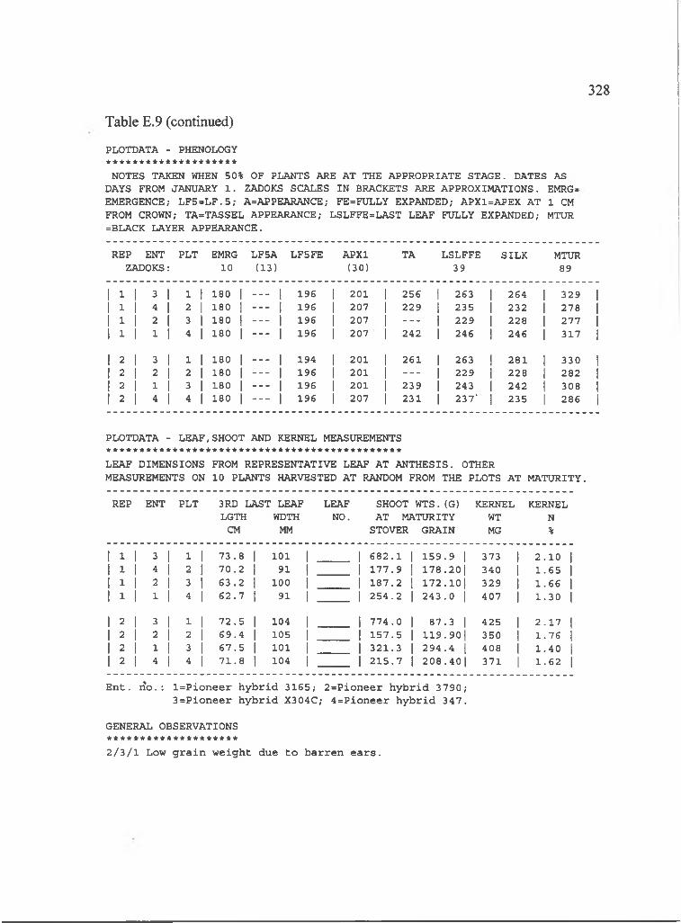
328
Table E.9 (continued)
PLOTDATA - PHENOLOGY * * * * * * * * * * * * * * * * * * * *
NOTES TAKEN WHEN 50% OF PLANTS ARE AT THE APPROPRIATE STAGE. DATES AS DAYS FROM JANUARY 1 . ZADOKS SCALES IN BRACKETS ARE APPROXIMATIONS. EMRG= EMERGENCE; L F5=LF .5 ; A=APPEARANCE; FE=FULLY EXPANDED; APX1=APEX AT 1 CM FROM CROWN; TA=TASSEL APPEARANCE; LSLFFE=LAST LEAF FULLY EXPANDED; MTUR =BLACK LAYER APPEARANCE.
REP ENT ZADOKS:
PLT EMRG10
LF5A(13)
LF5FE APXl(30)
TA LSLFFE39
SILK MTUR89
1 1 1 3 1 1 1 180 1 -----1 196 201 256 1 263 264 1 329 11 1 1 4 I 2 1 180 1 -----I 196 207 229 1 235 232 1 278 I1 1 1 2 1 3 I 180 1 ----- I 196 207 ---- I 229 228 I 277 I1 1 1 1 1 4 I 180 1 -----1 196 207 242 1 246 246 1 317 1
1 2 I 3 1 1 1 180 1 __ 1 194 201 261 1 263 281 1 330 11 2 1 2 1 2 I 180 I -----1 196 201 ---- 1 229 228 1 282 11 2 1 1 1 3 1 180 I ----1 196 201 239 I 243 242 I 308 I1 2 1 4 I 4 I 180 I ----1 196 207 231 1 237- 235 1 286 1
PLOTDATA - LEAF,SHOOT AND KERNEL MEASUREMENTS
LEAF DIMENSIONS FROM REPRESENTATIVE LEAF AT ANTHESIS. OTHER MEASUREMENTS ON 10 PLANTS HARVESTED AT RANDOM FROM THE PLOTS AT MATURITY.
REP ENT PLT 3RD LAST LEAF LGTH WDTH
CM MM
LEAFNO.
SHOOT WTS. (G) AT MATURITY
STOVER GRAIN
KERNELWTMG
KERNELN%
1 3 1 3 1 1 1 7 3 . 8 1 101 1 6 8 2 . 1 1 5 9 . 9 1 3 7 3 1 2 . 1 0 11 3 1 4 I 3 1 7 0 . 2 I 91 I 1 7 7 . 9 1 7 8 . 2 0 | 3 4 0 i 1 . 6 5 II 1 I 3 1 3 1 6 3 . 2 I 100 1 1 8 7 . 2 1 7 2 . 1 0 1 3 2 9 I 1 . 6 6 I1 3 1 1 I 4 I 6 2 . 7 1 91 1 2 5 4 . 2 2 4 3 . 0 I 4 0 7 I 1 . 3 0 I
1 3 1 3 1 1 1 7 2 . 5 1 104 1 7 7 4 . 0 8 7 . 3 1 4 2 5 1 2 . 1 7 11 3 1 3 1 3 1 6 9 . 4 I 1 0 5 1 1 5 7 . 5 1 1 9 . 9 0 | 3 5 0 I 1 . 7 6 I1 3 1 1 1 3 I 6 7 . 5 I 1 0 1 I 3 2 1 . 3 2 9 4 . 4 1 40 8 1 . 4 0 11 3 1 4 I 4 I 7 1 . 8 I 104 1 2 1 5 . 7 2 0 8 . 4 0 | 3 7 1 I 1 . 6 2 I
E n t. l i o . : l= P io n e e r h y b r id 3 1 6 5 ; 2 = P io n e e r h y b r id 3790 ;3 = P io n e e r h y b r id X304C; 4 = P io n e e r h y b r id 3 47 .
GENERAL OBSERVATIONS **■****■*■*♦■*■*******■***2 /3 / 1 Low g r a in w e ig h t due t o b a rre n e a r s .
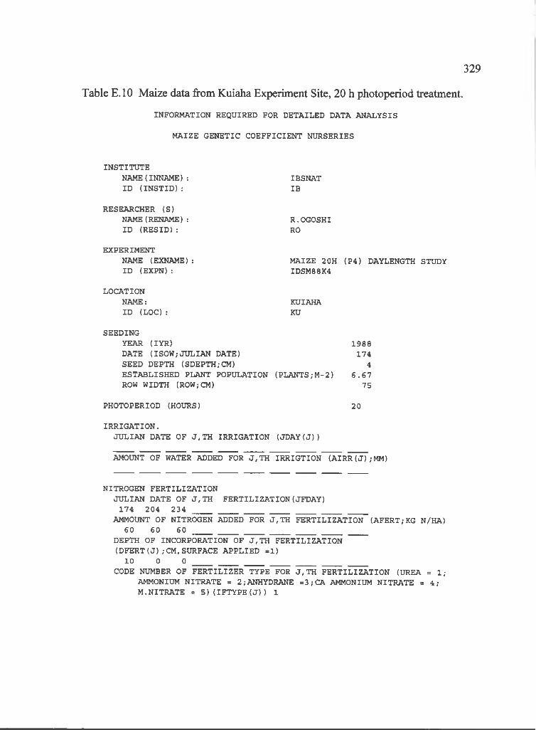
INFORMATION REQUIRED FOR DETAILED DATA ANALYSIS
MAIZE GENETIC COEFFICIENT NURSERIES
329
Table E.IO Maize data from Kuiaha Experiment Site, 20 h photoperiod treatment.
INSTITUTENAME( INNAME) : IBSNATID (IN S T ID ): IB
RESEARCHER (S)NAME(RENAME) : R . OGOSHIID (R E SID ): RO
EXPERIMENTNAME (EXNAME): MAIZE 2 OH (P4) DAYLENGTH STUDYID (EXPN): IDSM88K4
LOCATIONNAME: KUIAHAID (LO C ): KU
SEEDINGYEAR (lYR ) 1988DATE (ISOW,-JULIAN DATE) 174SEED DEPTH (SDEPTH,-CM) 4ESTABLISHED PLANT POPULATION (PLANTS,-M-2) 6 .6 7ROW WIDTH (ROW;CM) 75
PHOTOPERIOD (HOURS) 20
IRRIGATION.JULIAN DATE OF J,TH IRRIGATION (JD AY(J))
AMOUNT OF WATER ADDED FOR J,TH IRRIGTION (AIRR (J) ,-MM)
NITROGEN FERTILIZATIONJULIAN DATE OF J,TH FERTILIZATION(JFDAY)
174 204 234AMMOUNT OF NITROGEN ADDED FOR J,TH FERTILIZATION (AFERT,-KG N/HA)
60 60 60 ______________________________________________DEPTH OF INCORPORATION OF J,TH FERTILIZATION (DFERT (J ) ,-CM, SURFACE APPLIED =1)10 0 0
CODE NUMBER OF FERTILIZER TYPE FOR J,TH FERTILIZATION (UREA = 1;AMMONIUM NITRATE = 2,-ANHYDRANE =3;CA AMMONIUM NITRATE = 4;M.NITRATE = 5)(IFTYPE(J)) 1
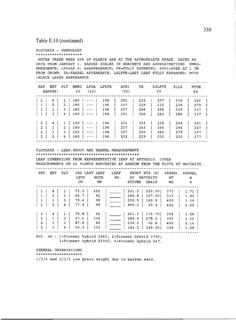
330
Table E.IO (continued)
PLOTDATA - PHENOLOGY * * * * * * * * * * * * * * * * * * * *
NOTES TAKEN WHEN 50% OF PLANTS ARE AT THE APPROPRIATE STAGE. DATES AS DAYS FROM JANUARY 1 . ZADOKS SCALES IN BRACKETS ARE APPROXIMATIONS. EMRG= EMERGENCE; L F5=LF .5 ; A=APPEARANCE; FE=FULLY EXPANDED; APX1=APEX AT 1 CM FROM CROWN; TA=TASSEL APPEARANCE; LSLFFE=LAST LEAF FULLY EXPANDED; MTUR =BLACK LAYER APPEARANCE.
REP ENT ZADOKS:
PLT EMRG10
LF5A(13)
LF5FE APXl(30)
TA LSLFFE39
SILK MTUR89
1 1 1 4 1 1 1 180 1 ----1 196 1 201 1 232 1 237 236 1 292 11 1 1 2 1 2 1 180 1 ----1 196 I 207 1 229 I 230 230 I 279 I1 1 1 1 1 3 I 180 I ----1 196 I 207 I 246 1 250 249 1 317 I1 1 1 3 I 4 1 180 I ----1 194 t 201 I 256 I 263 286 1 337 I
1 2 1 4 1 1 1 180 1 __ 1 196 1 201 1 233 1 238 238 1 301 11 2 1 1 1 2 1 180 I ----1 196 I 207 I 243 I 246 246 1 317 I1 2 1 3 I 3 I 180 1 ----1 194 1 207 I 256 1 263 279 1 337 1I 2 I 2 1 4 I 180 1 ----1 196 1 201 I 229 1 232 230 I 277 1
PLOTDATA - LEAF,SHOOT AND KERNEL MEASUREMENTS
LEAF DIMENSIONS FROM REPRESENTATIVE LEAF AT ANTHESIS. OTHER MEASUREMENTS ON 10 PLANTS HARVESTED AT RANDOM FROM THE PLOTS AT MATURITY.
REP ENT PLT 3RD LASI LGTH
CM
' LEAF WDTH
MM
LEAFNO.
SHOOT WTS.(G) AT MATURITY
STOVER GRAIN
KERNELWTMG
KERNELN%
1 1 1 4 1 1 I 7 3 .3 1 102 1 2 9 1 .0 2 2 9 .00| 373 1 1 .7 1 11 1 1 2 1 2 1 6 4 .7 1 92 I 1 8 5 .8 1 6 7 .00| 313 1 1 .9 0 I1 1 1 1 I 3 I 7 5 .4 1 98 1 2 0 8 .5 1 8 9 .9 1 400 I 1 .3 4 11 1 1 3 I 4 I 7 7 .9 I 99 I 4 4 9 .0 2 9 .9 I 422 I 2 .2 9 I
1 3 1 4 1 1 1 7 9 .8 1 92 1 2 0 1 .3 174 .701 304 1 1 .5 8 11 3 1 1 I 2 I 6 7 .6 I 102 1 2 8 9 .9 2 7 5 .0 1 393 1 1 .3 5 I1 3 1 3 I 3 I 8 7 .8 I 86 I 6 3 6 .0 6 6 .8 I 406 I 2 .1 6 I1 2 1 3 1 4 1 6 5 .9 I 103 1 1 4 1 .3 1 2 8 .20| 328 I 1 .8 8 I
E n t. n o . : l= P io n e e r h y b r id 3 1 6 5 ; 2 = P io n e e r h y b r id 3 7 9 0 ;3 = P io n e e r h y b r id X304C; 4 = P io n e e r h y b r id 3 4 7 .
GENERAL OBSERVATIONS
1 /3 /4 and 2 /3 /3 Low g r a in w e ig h t due t o b a r r e n e a r s .

331
APPENDIX F Maize data, winter 1988
Table F.l Maize data from Haleakala Experiment Station, control photoperiod treatment.
IBSNAT REDUCED DATA SET FOR MODELLING CROP GROWTH AND DEVELOPMENT PLOTDATA REQUIRED FOR FIELD EXPERIMENTS
GENERAL
PERSONNELRESEARCHER:INSTITUTION:
R ich a rd O gosh i IBSNAT
EXPERIMENT TITLE: ID :
IBSNAT DAYLENGTH;WINTER;MAIZE 1989 IDWM89H0
TREATMENTSGENOTYPES: 5MANAGEMENT: 0
LOCATIONNAME: HALEAKALA
PLOTS*****
PLANTING DATE
PLANT DENSITY (PLANTS/M2)
D ec. 2 8 , 1988
6 .6 7
ORGANISATIONNO.OF ROWS { # ) : 2ROW LENGTH (M ): 3ROW SPACING (CM): 75ORIENTATION OF ROWS: E-WALONG OR ACROSS DRAINS: n .a .SPACE BETWEEN PLOTS (CM ): 0GROSS AREA ( M 2 ) : 4 .5
HARVESTNO.OF ROWS: ROW LENGTH (M) AREA ( M 2 ) : METHOD:
121 .5hand
RANDOMIZATION/REPLICATIONDESIGN: RCBNO.OF REPS.-SOWN: 2
-HARVESTED: 2
PROBLEMS********
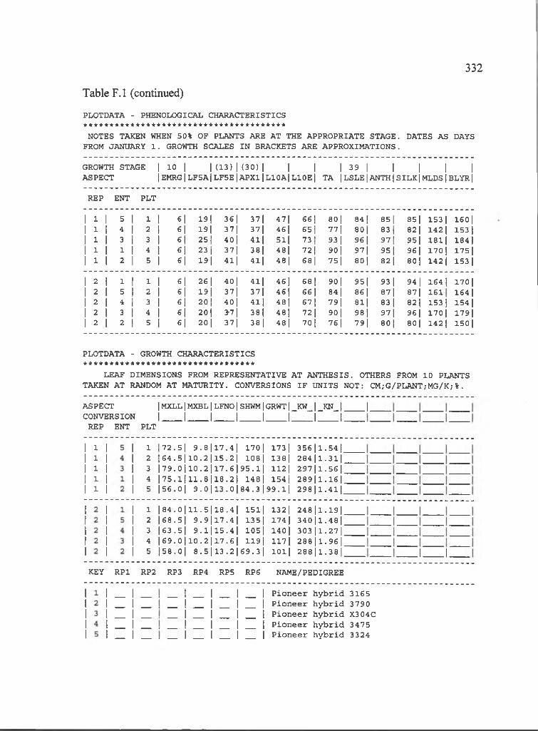
332
PLOTDATA - PHENOLOGICAL CHARACTERISTICS
NOTES TAKEN WHEN 50% OF PLANTS ARE AT THE APPROPRIATE STAGE. DATES AS DAYS FROM JANUARY 1 . GROWTH SCALES IN BRACKETS ARE APPROXIMATIONS.
GROWTH STAGE | 10 | |( 1 3 ) |( 3 0 ) | | | 1 39 | | | | |ASPECT |EMRG|LF5A|LF5E|APX1|L10A|L10E| TA |LSLE|ANTH|SILK|MLDS|BLYR|
REP ENT PLT
Table F.l (continued)
1 1 1 5 1 1 1 6| 19 1 36| 37| 47| 66 1 80 1 84 1 85| 851 153 1 160 11 1 1 4 I 2 1 6| 19| 37| 37| 46| 651 77 1 80l 831 821 142 1 153 11 1 1 3 1 3 1 6| 25 1 40| 41| 51| 73 1 93 1 961 971 951 181| 184 11 1 1 1 I 4 1 6| 23 1 37| 38| 48| 721 90 1 971 951 96 1 170 I 175 11 1 1 2 j 5 1 6| 19| 41| 41| 48| 68| 751 80l 82 1 80 1 142 1 153 1
1 2 1 1 1 1 1 6| 26 1 40 1 41| 461 68 1 90 1 951 93 1 94 1 164 1 170 11 2 1 5 I 2 1 6| 19 1 37| 37| 46| 66 I 84 1 86l 871 871 161 164 I1 3 1 4 1 3 1 6| 20 1 40 1 41| 481 67 1 791 81| 83 1 82 1 153! 154 I1 3 1 3 I 4 1 6| 20 I 37 1 38| 481 721 90 1 98l 97 1 96 1 1701 179 I1 2 1 2 1 5 1 6| 20| 37| 38| 481 70 1 76 1 79| 80l 80 1 142 1 150 I
PLOTDATA - GROWTH CHARACTERISTICS *********************************
LEAF DIMENSIONS FROM REPRESENTATIVE AT ANTHESIS. OTHERS FROM 10 PLANTS TAKEN AT RANDOM AT MATURITY. CONVERSIONS IF UNITS NOT: CM;G/PLANT;MG/K;%.
ASPECT IMXLL|MXBL|LFNO|SHWM|GRWT|_KW_|_KN_|CONVERSION I I I I I I I I
REP ENT PLT
J .
1 |72.5| 9 .8 | 1 7 .4 | 1 7 0 | 1 7 3 | 3 5 6 | l.5 4 |2 1 6 4 .5 | 1 0 .2 | 1 5 .2 | 1 0 8 j 138| 2 8 4 | l.3 l|3 | 7 9 .0 | 1 0 .2 | 1 7 .6 | 9 5 .1 | 1 1 2 | 2 9 7 | l.5 6 |4 | 7 5 . l | l l . 8 i l 8 .2 | 148| 1 5 4 j 2 8 9 | l.l6 |5 |56.0| 9 .0 | l 3 .0 | 8 4 .3 | 9 9 . l l 2 9 8 | l.4 l|
1 | 8 4 .0 | 1 1 .5 | 1 8 .4 | 15l| 132| 2 4 8 l l . l 9 |2 |68.5| 9 .9 | 1 7 .4 | 135| 1 7 4 j 3 4 0 | l.4 8 |3 |63.5| 9 .1 | 1 5 .4 | 105| 1 4 0 j 3 0 3 | l.2 7 |4 | 6 9 .0 | 1 0 .2 | 1 7 .6 | 1 1 9 j 1 1 7 j 2 8 8 | l.9 6 |5 |58.0| 8 .5 | 1 3 .2 | 6 9 .3 | lO l j 2 8 8 | l.3 8 | J I.
KEY RPl RP2 RP3 RP4 RP5 RP6 NAME/PEDIGREE
1 __ I I I P io n e e r h y b r id 3165I __ I I I P io n e e r h y b r id 3790I __ I I I P io n e e r h y b r id X304CI __ I I I P io n e e r h y b r id 3475I __ I I I P io n e e r h y b r id 3324
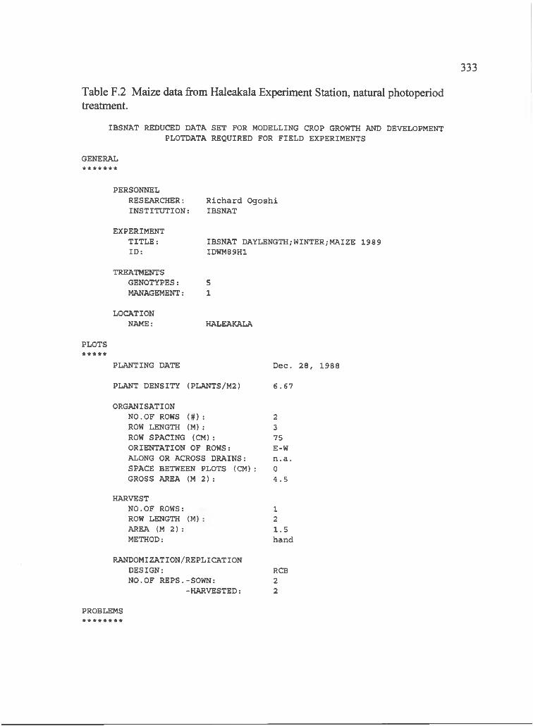
333
IBSNAT REDUCED DATA SET FOR MODELLING CROP GROWTH AND DEVELOPMENT PLOTDATA REQUIRED FOR FIELD EXPERIMENTS
GENERAL
Table F.2 Maize data from Haleakala Experiment Station, natural photoperiodtreatment.
PERSONNELRESEARCHER:INSTITUTION:
R ich a rd O gosh i IBSNAT
EXPERIMENT TITLE: ID :
IBSNAT DAYLENGTH;WINTER;MAIZE 1989 IDWM89H1
TREATMENTSGENOTYPES: 5MANAGEMENT: 1
LOCATIONNAME: HALEAKALA
PLOTS* * * * *
PLANTING DATE
PLANT DENSITY (PLANTS/M2)
D ec. 2 8 , 1988
6 .6 7
ORGANISATIONNO.OF ROWS ( # ) : 2ROW LENGTH (M ): 3ROW SPACING (CM ): 75ORIENTATION OF ROWS: E-WALONG OR ACROSS DRAINS: n .a .SPACE BETWEEN PLOTS (CM ): 0GROSS AREA ( M 2 ) : 4 .5
HARVESTNO.OF ROWS: ROW LENGTH (M) AREA ( M 2 ) : METHOD:
121 .5hand
RANDOMIZATION/REPLICATIONDESIGN: RCBNO.OF REPS.-SOWN: 2
-HARVESTED: 2
PROBLEMS********
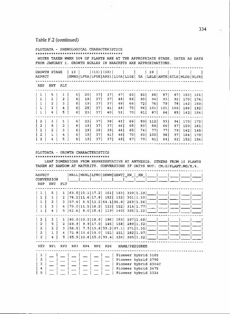
334
PLOTDATA - PHENOLOGICAL CHARACTERISTICS
Table F.2 (continued)
NOTES TAKEN WHEN 50% OF PLANTS ARE AT THE APPROPRIATE STAGE. DATES AS DAYS FROM JANUARY 1 . GROWTH SCALES IN BRACKETS ARE APPROXIMATIONS.
GROWTH STAGE | 10 | |( 1 3 ) |( 3 0 ) | | | | 39 | | | | |ASPECT |EMRG|LF5A|LF5E|APXljL10A|L10E| TA |LSLEj ANTH|SILK|MLDSjBLYR|
REP ENT PLT
1 1 1 5 1 1 1 e| 20 1 37| 371 471 651 83 1 881 871 87 1 153 1 16111 1 1 1 I 2 1 6| 19| 371 371 481 66 1 90 1 94 1 93 1 93 1 1701 174 11 1 1 2 1 3 1 6| 19 1 371 37| 481 66 1 72 1 76 1 791 78 1 142 I 150 11 1 1 3 I 4 1 6| 251 371 41| 481 701 96 1 1011 lO ll 100 1 188 1 192 11 1 1 4 I 5 1 6| 23 1 371 40l 51| 701 81| 871 84 1 851 142 1 154 I
1 2 1 3 1 1 1 6| 221 371 38| 41| 661 89l 112 1 93 1 94 1 1701 172 11 2 1 5 1 2 1 6| 19 I 371 371 46 1 651 83 1 88| 86 1 871 159 I 16111 2 1 2 1 3 1 6| 19 1 381 391 46 1 651 74 1 771 771 791 142 1 145|1 2 1 1 1 4 1 6| 19| 371 41| 481 70 1 93 1 lOOl 96 1 97 1 164 I 170 11 2 1 4 1 5 1 6| 19| 371 371 481 671 791 81| 84 1 821 152 1 154 1
PLOTDATA - GROWTH CHARACTERISTICS *********************************
LEAF DIMENSIONS FROM REPRESENTATIVE AT ANTHESIS. OTHERS FROM 10 PLANTS TAKEN AT RANDOM AT MATURITY. CONVERSIONS IF UNITS NOT: CM;G/PLANT;MG/K;%.
AS PECT IMXLL|MXBL|LFNO|SHWM|GRWT|_KW_|_KN_|CONVERSION I I I I I I I I
REP ENT PLT
.1
1 | 6 9 .5 | 1 0 .1 | 1 7 .2 | 161| 183| 3 2 9 | l.3 9 |2 | 7 8 .2 | l l .6 | l 7 .8 l 1 5 2 j 132| 3 0 l| l .3 3 |3 | 5 7 .4 l 8 .5 l l3 .2 | 6 4 . l| 9 6 .8 | 2 6 9 | l.3 6 |4 | 7 9 .0 | l l .5 | l 8 .2 i 123| 152| 3 1 4 | l.7 7 |5 [ 6 2 .6| 8 .0 | 1 5 .4 1 119| 140| 3 0 5 | l.3 3 |
1 | 8 0 .0 | 1 0 .2 | 1 8 .6 | 1861 1531 2 9 7 l l .6 8 l2 |69.9| 9 .9 | 1 7 .0 | 1451 1 5 8 j 2 8 9 | l.3 2 |3 |56.5| 7 .5 | 1 3 .6 | 5 9 .2 | 9 7 .1 | 2 7 l| l .3 5 |4 | 7 3 .8 | 1 0 .6 | 1 8 .0 | 1 5 1 j 15l| 2 8 2 | l.0 7 |5 | 6 5 .5 | l0 .6 | l5 .0 l9 9 .4 | 1261 2 8 5 | l.3 2 |
J I.
1 __ 1 1 1 P io n e e r h y b r id 3165I __ I I I P io n e e r h y b r id 3790I __ I 1 I P io n e e r h y b r id X304CI __ 1 I I P io n e e r h y b r id 3475I __ 1 I 1 P io n e e r h y b r id 3324
KEY RPl RP2 RP3 RP4 RP5 RP6 NAME/PEDIGREE

335
IBSNAT REDUCED DATA SET FOR MODELLING CROP GROWTH AND DEVELOPMENT PLOTDATA REQUIRED FOR FIELD EXPERIMENTS
Table F.3 Maize data from Kuiaha Experiment Site, control photoperiod treatment.
GENERAL
PERSONNELRESEARCHER:INSTITUTION:
R ich a rd O gosh i IBSNAT
EXPERIMENT TITLE: ID :
IBSNAT DAYLENGTH;WINTER;MAIZE 1989 IDWM89K0
TREATMENTSGENOTYPES: 5MANAGEMENT: 0
LOCATIONNAME: KUIAHA
PLOTS** * * *
PLANTING DATE
PLANT DENSITY (PLANTS/M2)
D ec. 2 9 , 1988
6 .6 7
ORGANISATIONNO.OF ROWS ( # ) : 2ROW LENGTH (M ): 3ROW SPACING (CM ): 75ORIENTATION OF ROWS: E-WALONG OR ACROSS DRAINS: n .a .SPACE BETWEEN PLOTS (CM ): 0GROSS AREA ( M 2 ) : 4 .5
HARVESTNO.OF ROWS: ROW LENGTH (M) AREA ( M 2 ) : METHOD:
121 .5hand
RANDOMIZATION/REPLICATIONDESIGN: RCBNO.OF REPS.-SOWN: 2
-HARVESTED: 2
PROBLEMS********
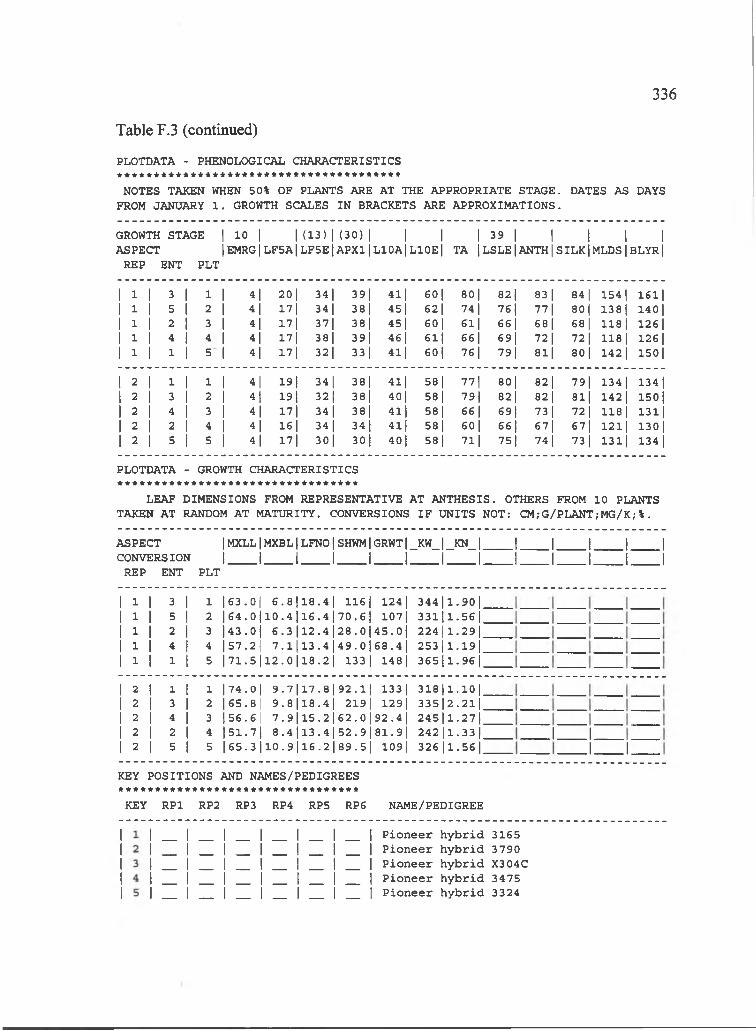
336
PLOTDATA - PHENOLOGICAL CHARACTERISTICS
Table F.3 (continued)
NOTES TAKEN WHEN 50% OF PLANTS ARE AT THE APPROPRIATE STAGE. DATES AS DAYS FROM JANUARY 1 . GROWTH SCALES IN BRACKETS ARE APPROXIMATIONS.
GROWTH STAGE | 10 | |( 1 3 ) |( 3 0 ) | | | | 39 | | j [ |ASPECT lEMRG|LF5A|LF5ElAPXl|L10A|L10E| TA jLSLEjANTH|SILK|MLDSjBLYRj
REP ENT PLT
1 1 3 1 1 1 4| 20| 341 391 411 60 1 80 1 821 83 1 84 1 154 1 16111 1 5 1 2 1 4| 17 1 341 38| 451 62 1 74 1 761 771 80l 1381 140 I1 1 2 1 3 1 4| 17 1 371 381 451 60| 611 66l 68 1 68 I 118 1 126 11 1 4 1 4 1 4| 17 1 381 391 46 1 611 661 691 72 1 721 118 1 126 I1 1 1 1 5 | 4| 17 1 321 33 1 411 60| 76 1 791 811 80| 142 I 150 I
2 1 1 1 1 1 4| 191 34 1 381 411 581 77| 80l 82 1 791 134 1 134 12 I 3 1 2 1 41 191 321 38| 40| 581 791 821 82 1 811 142 I 150 12 1 4 1 3 1 4| 17 1 34| 38| 411 58| 66 1 69| 73 1 72 1 118 I 13112 1 2 I 4 1 4| 16 1 34 1 34 1 411 581 60 I 66l 671 67| 1211 130 12 1 5 j 5 1 4| 17 1 301 301 40| 581 711 75| 74 1 73 1 1311 134 I
PLOTDATA - GROWTH CHARACTERISTICS * * * * * * * * * * * * * * * * * * * * * * * * * * * * * * * * *
LEAF DIMENSIONS FROM REPRESENTATIVE AT ANTHESIS. OTHERS FROM 10 PLANTS TAKEN AT RANDOM AT MATURITY. CONVERSIONS IF UNITS NOT: CM; G/PLANT;MG/K;%.
AS PECT I MXLL | MXBL | LFNO | SHWM | GRWT | _KW_ | _KN_ |______|______|______ |______|_____ |CONVERSION 1 I I I I 1 I I______1______I______ I______I_____ I
REP ENT PLT
1 1 3 1 1 |63.0| 6 .8 | 1 8 .4 | 116{1 124 1 3 4 4 | l.9 0 |1 1 5 I 2 |64.0|jlO .4 | 1 6 .4 | 7 0 .6 | 1 107| 331||1.56|1 1 2 1 3 |43.0|1 6 .3 | 1 2 .4 | 2 8 .0 | 4 5 .0 | 224 I1.29|1 1 4 1 4 157.21 7 . l j l 3 .4 | 4 9 .0 l 6 8 .4 | 253 11.19|1 I 1 1 5 | 7 1 .5 | 1 2 .0 | 1 8 .2 | 133|I 148| 365||1.96|
2 1 1 1 1 |74.0|1 9 .7 | 1 7 .8 | 9 2 .1 | j 133 1 318|( i . i o l2 1 3 1 2 |65.8| 9 .8 | 1 8 .4 | 219 1 129| 335||2.21|2 1 4 1 3 |56.6| 7 .9 | 1 5 .2 | 6 2 .0 |92.4| 245|| l.2 7 l2 1 2 1 4 |51.7|I 8 .4 | 1 3 .4 | 5 2 .9 181.91 242 |1.33|2 1 5 1 5 |65.3|| 1 0 .9 | 1 6 .2 | 8 9 .5 1 109 1 326 |1.56|
J I.J I.
KEY POSITIONS AND NAMES/PEDIGREES *********************************
KEY RPl RP2 RP3 RP4 RP5 RP6 NAME/PEDIGREE
P io n e e rP io n e e rP io n e e rP io n e e rP io n e e r
h y b r id 3165 h y b r id 3790 h y b r id X304C h y b r id 3475 h y b r id 3324

337
IBSNAT REDUCED DATA SET FOR MODELLING CROP GROWTH AND DEVELOPMENT PLOTDATA REQUIRED FOR FIELD EXPERIMENTS
Table F.4 M aize data from Kuiaha Experiment Site, natural photoperiod treatment.
GENERAL
PERSONNELRESEARCHER:INSTITUTION:
R ich a rd O gosh i IBSNAT
EXPERIMENT TITLE: ID :
IBSNAT DAYLENGTH/WINTER;MAIZE 1989 IDWM89K1
TREATMENTSGENOTYPES: 5MANAGEMENT: 1
LOCATIONNAME: KUIAHA
PLOTS* * * * *
PLANTING DATE
PLANT DENSITY (PLANTS/M2)
D ec. 2 9 , 1988
6 .6 7
ORGANISATIONNO.OF ROWS ( # ) : 2ROW LENGTH (M ): 3ROW SPACING (CM ): 75ORIENTATION OF ROWS: E-WALONG OR ACROSS DRAINS: n .a .SPACE BETWEEN PLOTS (CM) : 0GROSS AREA ( M 2 ) : 4 .5
HARVESTNO.OF ROWS: ROW LENGTH (M) AREA ( M 2 ) : METHOD:
121 .5hand
RANDOMIZATION/REPLICATIONDESIGN: RCBNO.OF REPS.-SOWN: 2
-HARVESTED: 2
PROBLEMS********
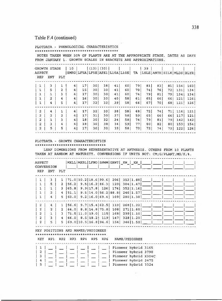
338
Table F.4 (continued)
PLOTDATA - PHENOLOGICAL CHARACTERISTICS
NOTES TAKEN WHEN 50% OF PLANTS ARE AT THE APPROPRIATE STAGE. DATES AS DAYS FROM JANUARY 1 . GROWTH SCALES IN BRACKETS ARE APPROXIMATIONS.
GROWTH STAGE | 10 | | (1 3 )1 (3 0 ) | I I ! 3 9 | | 1 | |ASPECT |E M R G |L F 5A |L F 5E |A P X 1|L 10A |L 10E | TA jLSLE|ANTHjSILK|M LDSjBLYRj
REP ENT PLT
1 1 3 1 1 1 4| 17 1 301 381 4 l l 60l 791 811 83 1 81| 154 1 160 11 1 5 1 2 1 4| 15 1 301 301 411 60| 701 74 1 76 1 72 1 1311 134 11 1 1 I 3 1 4| 17 1 301 301 411 60| 74 1 791 8 l l 791 134 1 134 11 1 2 1 4 1 4| 161 30l 331 40l 58! 61| 651 66 1 66 1 121! 126 11 1 4 I 5 1 4| 17! 321 33 1 391 58 1 66l 671 70 1 68| 1211 126 I
2 1 1 1 1 4| 17| 32| 33| 381 58 1 68l 721 74 1 711 116 1 121|2 1 2 1 2 1 4| 17| 31| 30! 371 581 59| 65| 661 66 1 117| 12112 1 1 1 3 1 4| 18 1 301 321 34 1 581 74 1 791 811 791 142 I 142 12 1 3 1 4 1 4| 18 1 301 381 341 59| 771 80l 82| 80l 153 1 154 I2 1 5 1 5 1 4| 17 1 301 301 391 581 70 1 721 74 1 72 1 122 1 126 I
PLOTDATA - GROWTH CHARACTERISTICS * * * * * * * * * * * * * * * * * * * * * * * * * * * * * * * * *
LEAF DIMENSIONS FROM REPRESENTATIVE AT ANTHESIS. OTHERS FROM 10 PLANTS TAKEN AT RANDOM AT MATURITY. CONVERSIONS IF UNITS NOT: CM;G/PLANT;MG/K;%.
ASPECT IMXLL|MXBL|LFNO|SHWM|GRWT|_KW_|_KN_|CONVERSION I I I I I I I I
REP ENT PLT
J ____I.J ____ I.
1 1 3 1 1 1 7 1 .o l i o . 2 l l 8 . 6 l 9 0 . 6 l 2061 3 5 3 1 1 .88l1 1 5 I 2 156.21 9 . 5 l l 6 . 2 l 8 6 . 3 l 120 1 3 0 4 l l .4 7 l1 1 1 1 3 165.81 9 .9 | l 7 .8 l 126] 1741 3 5 2 l l . l 6 l1 1 2 I 4 |51.1| 9 .5 11 4 .0 156 .2 I8 8 .8| 2 4 6 1 1 .57l1 1 4 1 5 160.01 9 .2 | 1 6 .0 | 6 9 .4 | 109| 2 8 0 l l .3 0 l
2 1 4 1 1 156.61 9 .7 1 1 5 .4 1 6 2 .5 1 i i o l 2 6 8 l l .2 2 l2 1 2 1 2 164.01 8 .8 11 4 .8 I 75 .81 108| 2 7 l l l . 6 0 l2 1 1 1 3 | 71 .5 l 1 1 .0 l l9 .0 | 115| 168 I 2 9 9 1 1 .lO l2 1 3 1 4 1 66 .01 8 .5 | l 8 .2 t 119| 147| 3 2 8 1 1 .20l2 1 5 1 5 I 6 9 . 0 l l 0 . 5 l l 6 . 8 l 9 4 . 6 l 154 I 3 4 6 l l .5 0 l
.1____ I.J ____I.J ____I.J ____I.
KEY POSITIONS AND NAMES/PEDIGREES * * * * * * * * * * * * * * * * * * * * * * * * * * * * * * * * *
KEY RPl RP2 RP3 RP4 RP5 RP6 NAME/PEDIGREE
P io n e e rP io n e e rP io n e e rP io n e e rP io n e e r
h y b r id 3165 h y b r id 3790 h y b r id X304C h y b r id 3475 h y b r id 3324

339
APPENDIX G Maize data, sununer 1989
Table G.l Maize data from Haleakala Experiment Station, control photoperiod treatment.
IBSNAT REDUCED DATA SET FOR MODELLING CROP GROWTH AND DEVELOPMENT PLOTDATA REQUIRED FOR FIELD EXPERIMENTS
GENERAL
PERSONNELRESEARCHER: INSTITUTION:
R ich a rd O gosh i IBSNAT
EXPERIMENT TITLE: ID :
IBSNAT DAYLENGTH;SUMMER;MAIZE 1989 IDSM89H0
TREATMENTSGENOTYPES: 5MANAGEMENT: 0
LOCATIONNAME: HALEAKALA
PLOTS*****
PLANTING DATE
PLANT DENSITY (PLANTS/M2)
S ep . 9 , 1989
6 .6 7
ORGANISATIONNO.OF ROWS ( # ) : 2ROW LENGTH (M ): 3ROW SPACING (CM ): 75ORIENTATION OF ROWS: E-WALONG OR ACROSS DRAINS: n .a .SPACE BETWEEN PLOTS (CM ): 75GROSS AREA ( M 2 ) : 4 .5
HARVESTNO.OF ROWS: ROW LENGTH (M) AREA (M 2 ) : METHOD:
121 .5hand
RANDOM IZATI ON/RE PL I CAT I ONDESIGN: RCBNO.OF REPS.-SOWN: 2
-HARVESTED: 2
PROBLEMS********
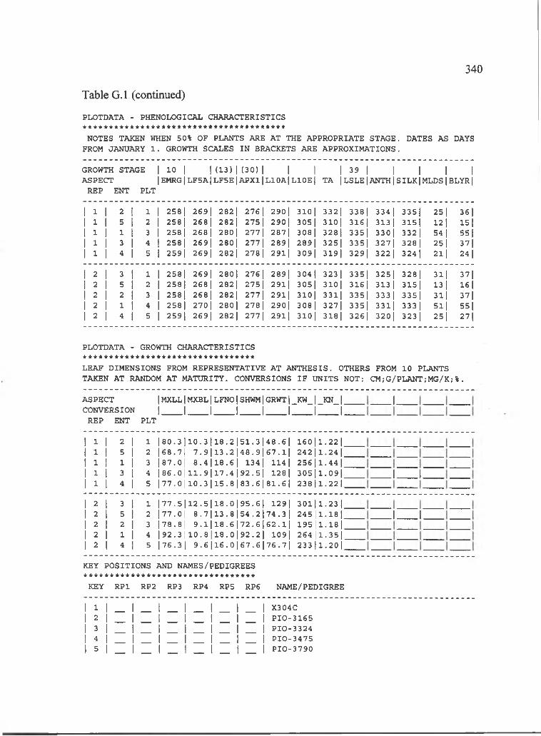
340
Table G.l (continued)
PLOTDATA - PHENOLOGICAL CHARACTERISTICS ***************************************
NOTES TAKEN WHEN 50% OF PLANTS ARE AT THE APPROPRIATE STAGE. DATES AS DAYS FROM JANUARY 1 . GROWTH SCALES IN BRACKETS ARE APPROXIMATIONS.
GROWTH STAGE | 10 | | (13) | (30) | | | | 39 | | | | |ASPECT |EMRG|LF5AlLF5E|APXl|L10A|L10E| TA jLSLEjANTH|SILKjMLDSjBLYRj
REP ENT PLT
1 1 2 1 1 1 258 1 269) 282) 276) 290) 310) 3321 338) 334 1 3351 251 36|1 1 5 1 2 1 258 1 268 I 282| 275) 290 I 305| 310) 316| 313 1 3151 12 1 15 11 1 1 1 3 1 258 1 268 I 280 I 277) 287| 308| 328) 3351 3301 3321 54 1 5511 1 3 1 4 1t 258 1 269| 280| 2771 289| 289| 3251 3351 3271 328) 25 1 3711 1 4 I 5 11 259| 269| 282 1 278) 29l| 309| 319) 329) 322 1 324 I 21| 24 1
2 1 3 1 1 11 258| 269) 280) 276) 289) 304) 323 1 3351 325) 328 1 31| 3713 1 5 1 2 11 258| 268| 282 I 275| 291| 305| 310) 3161 313 1 315| 13 1 1612 1 2 j 3 11 258 1 268 1 282 I 277 I 291| 310| 3311 3351 3331 3351 31| 3712 I 1 I 4 11 258| 270 I 280 1 278| 290| 308| 327) 3351 331| 3331 511 55 12 I 4 1 5 11 2591 269| 282 I 277 I 2 9 l l 310] 318| 326) 320) 323 1 251 271
PLOTDATA - GROWTH CHARACTERISTICS
LEAF DIMENSIONS FROM REPRESENTATIVE AT ANTHESIS. OTHERS FROM 10 PLANTS TAKEN AT RANDOM AT MATTOITY. CONVERSIONS IF UNITS NOT: CM;G/PLANT;MG/K;%.
ASPECT CONVERSION
REP ENT
IMXLLIMXBL|LFNO|SHWM|GRWT|_KW_|_KN_|I I I I I I I I
PLT
J .
1 1 3 1 1 1 8 0 .3|l l O .3 ) 1 8 .2 )5 1 .3 ) 4 8 .6 1 160| 1.2211 I 5 I 2 1 6 8 .7| 7 .9 | l3 .2 l 4 8 .9 | 6 7 . l | 242 11.3411 1 1 1 3 1 8 7 .0| 8 .4 | 1 8 .6 | 134| 114| 256 I| l-4 4 l1 1 3 I 4 l86 .0| 1 1 .9 | 1 7 .4 | 9 2 .5 | 128) 305||1.09|1 1 4 1 5 177.01 1 0 .3 | 1 5 .8 | 8 3 .6 | 8 1 .6 | 238|11.221
2 1 3 1 1 |77.5|| 1 2 .5 ) 1 8 .0 ) 9 5 .6 ) 129) 301|11 .33 )3 1 5 I 2 1 7 7 .0| 8 .7 11 3 .8 1 5 4 .2 )7 4 .3 I 245 11 .18 )3 1 3 1 3 1 7 8 .8| 9 . l | l 8 .6 | 7 2 .6 l 6 2 . l | 195 |1.1813 1 1 I 4 |93.3| 1 0 .8 | 1 8 .0 | 9 2 .2 | 109| 264 11-3513 1 4 1 5 |76.3 I 9 .6 l l6 .0 l6 7 .6 | 7 6 .7 | 2331|1.30|
J I.
J I.
KEY POSITIONS AND NAMES/PEDIGREES * * * * * * * * * * * * * * * * * * * * * * * * * * * * * * * * *
KEY RPl RP2 RP3 RP4 RP5 RP6 NAME/PEDIGREE
12345
X304CPIO -3165PIO -3324P IO -3475PIO -3790

341
IBSNAT REDUCED DATA SET FOR MODELLING CROP GROWTH AND DEVELOPMENT PLOTDATA REQUIRED FOR FIELD EXPERIMENTS
GENERAL* * * * * * *
Table G.2 Maize data from Haleakala Experiment Station, natural photoperiodtreatment.
PERSONNELRESEARCHER:INSTITUTION:
R ich a rd O gosh i IBSNAT
EXPERIMENT TITLE: ID :
IBSNAT DAYLENGTH/SUMMER;MAIZE 1989 IDSM89H1
TREATMENTSGENOTYPES: 5MANAGEMENT: 1
LOCATIONNAME: HALEAKALA
PLOTS* * * * *
PLANTING DATE
PLANT DENSITY (PLANT/M2)
S ep . 9 , 1989
6 .6 7
ORGANISATIONNO.OF ROWS ( # ) : 2ROW LENGTH (M ): 3ROW SPACING (CM ): 75ORIENTATION OF ROWS: E-WALONG OR ACROSS DRAINS: n .a .SPACE BETWEEN PLOTS (CM ): 0GROSS AREA ( M 2 ) : 4 .5
HARVESTNO.OF ROWS: ROW LENGTH (M) AREA (M 2 ) : METHOD:
121 .5hand
RANDOMIZATION/REPLICATIONDESIGN: RCBNO.OF REPS.-SOWN: 2
-HARVESTED: 2
PROBLEMS********
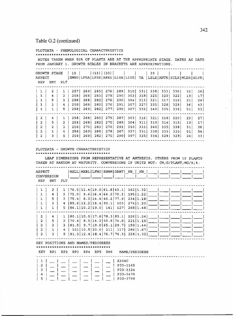
342
PLOTDATA - PHENOLOGICAL CHARACTERISTICS
Table G.2 (continued)
NOTES TAKEN WHEN 50% OF PLANTS ARE AT THE APPROPRIATE STAGE. DATES AS DAYS FROM JANUARY 1 . GROWTH SCALES IN BRACKETS ARE APPROXIMATIONS.
GROWTH STAGE | 10 | | (1 3 )| (3 0 )| | | | 39 | | | | |ASPECT |EMRG|LF5A|LF5E|APX1|L10A|L10E| TA jLSLEjANTHjSILK|MLDSjBLYR|
REP ENT PLT
1 1 2 1 1 1 257 1 269| 283 1 276 1 2891 310| 3311 338| 3331 335| 32| 3611 1 4 I 2 1 258 1 268 I 283 I 278| 290 1 303| 3181 3251 3201 3221 19| 17 11 1 5 I 3 11 258 1 268 1 282 1 2761 290 1 304 1 313 1 321| 3171 3181 21| 24 11 1 3 1 4 11 258 1 268 1 280| 276] 291| 3071 3271 3351 328 1 328 I 36| 4311 1 1 1 5 11 258| 269| 282 I 277| 290 I 3071 3321 3401 3351 338 1 51| 53 1
2 1 4 1 1 11 258 1 268| 283 1 275| 2871 303 1 3161 3211 3181 3201 23 1 27 12 I 5 1 2 11 258| 268| 282| 275 I 289| 304 I 311| 319| 314 I 315| 19| 1712 I 2 I 3 11 258| 270 I 283 I 276 I 291| 310| 333 1 340| 3351 3381 31| 36|2 I 1 I 4 11 258 1 269| 280| 278 I 2871 3071 3311 338 I 3331 3351 51| 54 12 1 3 1 5 i1 258 1 269| 282| 275| 290| 3071 3251 334 I 328 1 329 1 24 1 33 1
PLOTDATA - GROWTH CHARACTERISTICS *********************************
LEAF DIMENSIONS FROM REPRESENTATIVE AT ANTHESIS. OTHERS FROM 10 PLANTS TAKEN AT RANDOM AT MATURITY. CONVERSIONS IF UNITS NOT: CM; G/PLANT;M G/K;%.
ASPECT IMXLL|MXBL|LFNO|SHWM|GRWT|_KW_|_KN_|CONVERSION I I I I I I I I
REP ENT PLT
J
245 3 1
1 | 7 6 .5 | 1 1 .4 | 1 9 .0 | 6 1 .8 | 4 3 .1 | 1 6 2 | l.3 2 |2 |75.0| 9 .6 | 1 6 .4 | 6 4 .2 | 7 0 .3 | 1 9 5 | l.2 2 |3 |75.4| 8 .3 | 1 4 .4 | 4 6 .2 | 7 7 .9 | 2 3 4 | l.l8 |4 | 8 5 .6 | 1 2 .2 | 1 8 .4 | 9 0 .1 | 1 0 3 | 2 7 4 | l.2 0 |5 | 8 6 .1 | 1 0 .2 | 1 9 .0 | 141| 1 2 7 j 2 6 8 | l.4 6 |
1 | 8 0 .1 | 1 0 .0 | 1 7 .6 | 7 8 .3 | 8 3 .1 | 226| l.24| _2 |70.4| 8 .5 | 1 4 .2 | 5 5 .8 | 7 4 .8 | 2 2 l i l . l 9 | ^3 |81.5| 9 .7 | 1 9 .0 | 6 5 .1 | 2 9 .7 | 1 5 0 | l.4 4 | '4 1 1 0 1 | 1 0 .5| 20 .0| 211| 117| 2 8 6 | l.6 7 | ’5 | 8 1 .3 | 1 2 .4 | 1 8 .4 | 7 6 .7 | 7 6 .3 | 228|l.32|^
J ____ I.J ____I.
KEY POSITIONS AND NAMES/PEDIGREES * * * * * * * * * * * * * * * * * * * * * * * * * * * * * * * * *
KEY RPl RP2 RP3 RP4 RP5 RPG NAME/PEDIGREE
X304CP IO -3165PIO -3324PIO -3475PIO -3790

343
IBSNAT REDUCED DATA SET FOR MODELLING CROP GROWTH AND DEVELOPMENT PLOTDATA REQUIRED FOR FIELD EXPERIMENTS
GENERAL*******
Table G.3 Maize data from Haleakala Experiment Station, 14 h photoperiodtreatment.
PERSONNELRESEARCHER:INSTITUTION:
R ich a rd O gosh i IBSNAT
EXPERIMENT TITLE: ID :
IBSNAT DAYLENGTH;SUMMER;MAIZE 1989 IDSM89H2
TREATMENTSGENOTYPES: 5MANAGEMENT: 1
LOCATIONNAME: HALEAKALA
PLOTS*****PLANTING DATE
PLANT DENSITY (PLANTS/M2)
June 15 , 1989
6 .6 7
ORGANISATIONNO.OF ROWS ( # ) : 2ROW LENGTH (M ): 3ROW SPACING (CM ): 75ORIENTATION OF ROWS: E-WALONG OR ACROSS DRAINS: n .a .SPACE BETWEEN PLOTS (CM ): 0GROSS AREA ( M 2 ) : 4 .5
HARVESTNO.OF ROWS: ROW LENGTH (M) AREA (M 2 ) : METHOD:
121 .5hand
RANDOMIZATION/REPLICATIONDESIGN: RCBNO.OF REPS.-SOWN: 2
-HARVESTED: 2
PROBLEMS********
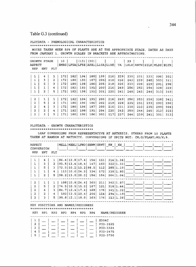
PLOTDATA - PHENOLOGICAL CHARACTERISTICS
Table G.3 (continued)
344
NOTES TAKEN WHEN 50% OF PLANTS ARE AT THE APPROPRIATE STAGE. DATES AS DAYS FROM JANUARY 1 . GROWTH SCALES IN BRACKETS ARE APPROXIMATIONS.
GROWTH STAGE | 10 | | (1 3 )| (3 0 )| | | | 39 | | | | [ASPECT |EMRG|LF5A|LF5E|APXllL10A|L10E| TA |LSLEjANTHjSILKjMLDS|BLYR|
REP ENT PLT
1 1 1 4 1 1 11 172 1 1821 194 1 188 1 1991 2161 2291 2351 2311 233 1 2961 3 0 ll1 1 1 3 1 2 11 1721 180| 193 1 187| 205 1 218| 236| 243 1 2391 240 I 303 1 311|1 1 1 5 I 3 11 172 1 180 I 198 1 186 I 205| 218 I 226 I 2331 228| 229| 2911 296 11 1 1 1 I 4 11 172 1 182 1 193 1 19l| 200 1 216| 249| 256 1 252 1 254 1 328 329|1 1 1 2 1 5 11 1721 182 1 198| 1 9 1 1 201| 220 I 241| 248| 243 1 244 I 313 1 319 I
1 2 1 1 1 1 11 172 1 182 1 194 1 1 9 ll 200 1 2161 2491 256 1 253 1 254 1 3381 34111 2 I 5 1 2 11 1711 180 1 196 1 186 1 202 I 219| 228 I 235| 2311 233 1 292 I 296]1 2 1 4 I 3 !1 172 1 180 1 196 1 1871 200| 216 I 2311 238| 233 1 2351 299| 304 I1 2 I 2 1 4 11 1711 182 1 198 I 1 9 l j 204 I 220| 2421 250 1 244 1 2451 313 1 31511 2 1 3 1 5 11 1711 180| 196 I 186 1 202 1 2171 2371 244 I 239| 241| 3011 313 1
PLOTDATA - GROWTH CHARACTERISTICS *********************************
LEAF DIMENSIONS FROM REPRESENTATIVE AT ANTHESIS. OTHERS FROM 10 PLANTS TAKEN AT RANDOM AT MATURITY. CONVERSIONS IF UNITS NOT: CM;G/PLANT;MG/K;%.
ASPECT IMXLL|MXBL|LFNO j SHWM|GRWT|_KW_|_KN_|CONVERSION I I I 1 I I I I
REP ENT PLT
J ____ I..1____ I.
1 1 8 6 .4 | 1 2 .8 | 1 7 .4 | 1 5 4 | 15l| 314|l.3G |2 | 9 3 .5 i l3 .4 | l8 .4 | 147| 160| 3 2 2 | l.3 3 |3 | 7 2 .5 | l0 .2 | l5 .2 | 9 8 .5 i 112| 2 8 5 | l.l9 |4 I 113| 1 0 .6 | 2 4 .2 | 334| 1721 3 3 8 ll .8 0 |5 | 9 8 .2 l l3 .0 | 2 0 .2 | 1 5 4 j 1541 2 6 4 ll .0 4 |
J ____I.J ____I.
1 1 1 0 8 1 1 0 .8 1 2 4 .4 1 3601 2 1 l l 3 4 2 l l .8 7 l2 | 7 4 .5 | 1 0 .5 | 1 5 .2 | 107| 12l| 3 1 8 | l .4 4 l ’3 | 8 4 .7 | 1 2 .4 | 1 7 .4 | 1 6 8 j 1 7 6 j 3 4 l| l.3 2 | ^4 1 1 0 2 | l2 .5 l2 0 .4 l 2 0 6 j 1 5 4 j 2 9 4 | l . l9 | '5 | 9 5 .8 | l 2 . l l l 8 . 0 l 169| 1 7 6 j 3 1 3 l l .3 8 | '
KEY POSITIONS AND NAMES/PEDIGREES * * * * * * * * * * * * * * * * * * * * * * * * * * * * * * * * *
KEY RPl RP2 RP3 RP4 RP5 RP6 NAME/PEDIGREE
12345
X304CP IO -3165PIO -3324PIO -3475PIO -3790
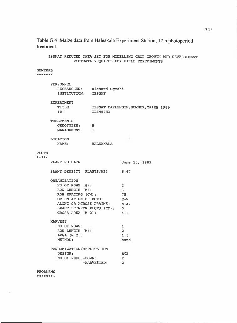
345
IBSNAT REDUCED DATA SET FOR MODELLING CROP GROWTH AND DEVELOPMENT PLOTDATA REQUIRED FOR FIELD EXPERIMENTS
GENERAL
Table G.4 Maize data from Haleakala Experiment Station, 17 h photoperiodtreatment.
PERSONNELRESEARCHER: INSTITUTION:
R ich a rd O gosh i IBSNAT
EXPERIMENT TITLE: ID :
IBSNAT DAYLENGTH;SUMMER;MAIZE 1989 IDSM89H3
TREATMENTSGENOTYPES: 5MANAGEMENT: 1
LOCATIONNAME: HALEAKALA
PLOTS* * * * *
PLANTING DATE
PLANT DENSITY (PLANTS/M2)
June 15 , 1989
6 .S 7
ORGANISATIONNO.OF ROWS ( # ) : 2ROW LENGTH (M ): 3ROW SPACING (CM ): 75ORIENTATION OF ROWS: E-WALONG OR ACROSS DRAINS: n .a .SPACE BETWEEN PLOTS (CM ): 0GROSS AREA ( M 2 ) : 4 .5
HARVESTNO.OF ROWS: ROW LENGTH (M) AREA ( M 2 ) : METHOD:
121 .5hand
RANDOMIZATION/REPLICATIONDESIGN: RCBNO.OF REPS.-SOWN: 2
-HARVESTED: 2
PROBLEMS********
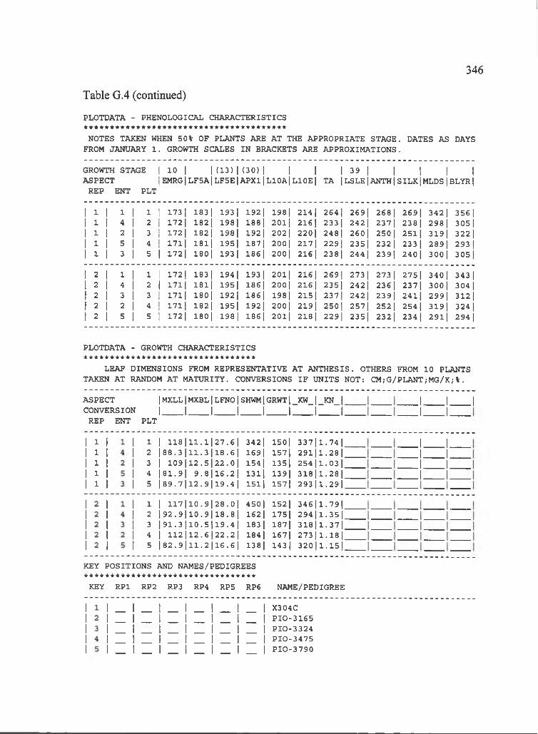
346
PLOTDATA - PHENOLOGICAL CHARACTERISTICS
Table G.4 (continued)
NOTES TAKEN WHEN 50% OF PLANTS ARE AT THE APPROPRIATE STAGE. DATES AS DAYS FROM JANUARY 1 . GROWTH SCALES IN BRACKETS ARE APPROXIMATIONS.
GROWTH STAGE 1 10 1 1 (13 ) 1 (30) 1 1 1 1 39 1 1 1 1 1ASPECT 1EMRG 1LF5A|LF5E|APX1|L10A|L10E| TA 1LSLElANTHl SILKl MLDSl BLYRl
REP ENT PLT
1 1 1 1 1 1 1 173 1 183 1 193 1 192 1 198 1 214 1 264 1 2691 268| 2691 342 1 356 11 1 1 4 I 2 1 172 1 182 I 198 I 188 I 201| 216 I 233 I 242 I 237| 238| 298 I 305 11 1 1 2 1 3 1 172 1 182 1 198| 192 I 202 I 220| 248 1 260 I 250| 2511 319| 322 11 1 1 5 I 4 1 1711 181| 195| 187| 200| 217| 229| 2351 232| 233 1 289| 293 11 1 1 3 1 5 11 1721 180| 193 I 186 I 200 1 216 1 238| 244 1 2391 240 1 300| 305|
1 2 1 1 1 1 1 172 1 183 1 194 1 193 1 201| 216 1 2691 273 1 273 1 2751 340 1 343 1I 2 I 4 I 2 11 1711 181| 195| 186 I 200| 216 1 235| 242| 236 1 2371 300| 304 II 2 1 3 I 3 1 1711 180| 192 I 186 I 198 I 2151 2371 242| 2391 2411 299| 312 1I 2 1 2 1 4 1 1711 182| 195| 192 I 200| 2191 2501 257| 252 I 254 I 319 I 3241I 2 1 5 1 5 1 172 1 180| 198 I 186 I 201| 218 I 229| 235| 232 I 234| 291| 294 I
PLOTDATA - GROWTH CHARACTERISTICS * * * * * * * * * * * * * * * * * * * * * * * * * * * * * * * * *
LEAF DIMENSIONS FROM REPRESENTATIVE AT ANTHESIS. OTHERS FROM 10 PLANTS TAKEN AT RANDOM AT MATURITY. CONVERSIONS IF UNITS NOT: CM;G/PLANT;MG/K;%.
ASPECT IMXLL|MXBL|LFNO|SHWM|GRWT[_KW_|_KN_|_CONVERSION I I I I I I I j'
REP ENT PLT
J ____I..1____ I.
.1
1 I 1 1 8 | 1 1 .1| 27 .6|2 | 8 8 .3 | 1 1 .3 | 1 8 .6 |3 I 1 09| 12 .5| 22 .0|4 |81.9| 9 .8 | 1 6 .2 |5 | 8 9 .7 | 1 2 .9 | 1 9 .4 |
342| 150| 337|1.74|_ 169| 157| 2 9 l l l . 2 8 | ' 154| 135| 254| l.03| _ 1 3 l j 139| 318|1.28|_ 15l| 157| 2 9 3 | 1 .2 9 | '
.1____I.J ____ I.J ____I.J ____I.
1 1 1 17| 10 .9| 28 .0|2 | 9 2 .9 | 1 0 .9 | 1 8 .8 |3 | 9 1 .3 t l0 .5 | l9 .4 |4 I 1 12| 12 .6| 22 .2|5 1 8 2 .9 1 1 1 .2|16.6|
450 I 152 I 162| 175| 183| 187| 184| 167| 138| 143|
3 4 6 | l.7 9 l_ 2 9 4 | l.3 5 | ' 3 1 8 | 1 .3 7 | ‘ 273 11 .1 8 I. 320 1 .1 5 l '
KEY POSITIONS AND NAMES/PEDIGREES * * * * * * * * * * * * * * * * * * * * * * * * * * * * * * * * *
KEY RPl RP2 RP3 RP4 RP5 RP6 NAME/PEDIGREE
X304CPIO -3165PIO -3324PIO -3475PIO -3790

347
IBSNAT REDUCED DATA SET FOR MODELLING CROP GROWTH AND DEVELOPMENT PLOTDATA REQUIRED FOR FIELD EXPERIMENTS
GENERAL*******
Table G.5 Maize data from Haleakala Experiment Station, 20 h photoperiodtreatment.
PERSONNELRESEARCHER:INSTITUTION:
R ich a rd O gosh i IBSNAT
EXPERIMENT TITLE: ID :
IBSNAT DAYLENGTH;SUMMER;MAIZE 1989 IDSM89H4
TREATMENTSGENOTYPES: 5MANAGEMENT: 1
LOCATIONNAME: HALEAKALA
PLOTS*****PLANTING DATE
PLANT DENSITY (PLANTS/M2)
June 15 , 1989
6 .67
ORGANISATIONNO.OF ROWS ( # ) : 2ROW LENGTH (M ): 3ROW SPACING (CM ): 75ORIENTATION OF ROWS: E-WALONG OR ACROSS DRAINS: n .a .SPACE BETWEEN PLOTS (CM ): 0GROSS AREA ( M 2 ) : 4 .5
HARVESTNO.OF ROWS: ROW LENGTH (M) AREA ( M 2 ) : METHOD:
121 .5hand
RANDOMIZATION/REPLICATIONDESIGN: RCBNO.OF REPS.-SOWN: 2
-HARVESTED: 2
PROBLEMS********

348
PLOTDATA - PHENOLOGICAL CHARACTERISTICS
Table G.5 (continued)
NOTES TAKEN WHEN 50% OF PLANTS ARE AT THE APPROPRIATE STAGE. DATES AS DAYS FROM JANUARY 1 . GROWTH SCALES IN BRACKETS ARE APPROXIMATIONS.
GROWTH STAGE | 10 | |( 1 3 ) |( 3 0 ) | | | | 39 | | | | |ASPECT 1EMRG|LF5A|LF5E|APX1|L10A|L10E| TA |LSLEjANTHjSILKjMLDS|BLYRj
REP ENT PLT
1 1 2 1 1 11 172| 183 1 198 1 19l| 202 1 221| 2511 258 1 253 1 254 1 325| 33311 1 5 1 2 11 172 1 18l| 198 1 1911 203| 219| 231| 24l| 2331 235| 29l| 294 11 1 3 I 3 11 1711 182 I 196 I 192 I 202| 219| 242 I 249| 244 1 247| 300| 318 11 1 4 I 4 11 172 1 182 1 198 I 192 I 205| 220 1 238| 245 1 241| 244 1 312 1 314 11 1 1 I 5 11 172 1 183 1 196 1 193 1 20l| 216 1 270 I 279| 2751 277| 342 1 363 1
2 1 5 1 1 11 1711 180| 194 1 186 1 198| 216 1 231| 236| 2321 234| 291| 296|2 I 2 I 2 1 1 7 1 1 183 1 198 1 191| 200| 219 j 252 1 2 6 l j 254 1 254 1 325| 335|2 I 3 I 3 1 1711 180| 193 1 188 1 200| 216| 242 1 248 1 244 I 245| 312| 31512 I 4 I 4 1 172 1 1 8 l j 195| 187| 200| 2161 237| 244 I 240| 241| 300| 304 12 I 1 1 5 1 172 1 183 1 196 I 193 I 201| 217| 273 1 279| 276 1 278| 341| 363 1
PLOTDATA - GROWTH CHARACTERISTICS * * * * * * * * * * * * * * * * * * * * * * * * * * * * * * * * *
LEAF DIMENSIONS FROM REPRESENTATIVE AT ANTHESIS. OTHERS FROM 10 PLANTS TAKEN AT RANDOM AT MATURITY. CONVERSIONS IF UNITS NOT: CM;G/PLANT;MG/K;%.
ASPECT CONVERSION
REP ENT
IMXLLIMXBL|LFNO|SHWM|GRWT|_KW_|_KN_| . 1. J
PLT
1 1 2 1 1 1 1 0 6 | 1 3 .3| 21 .6| 176 1 149| 266|1.13|1 1 5 1 2 | 8 3 .4 | 1 1 .1 | 1 6 .4 | 143 1 134 j 308|1.13|1 1 3 I 3 j 94 . 9 j i 2 . 0 j i 9 . 0 j 167j 159j 3 0 2 | l .2 6 l1 I 4 1 4 j 93 . 5 j i 2 . 0 j l 8 . 6 j 117 1 147 j 2 4 9 | l.2 9 |1 I 1 I 5 1 i 25 j l l . 5 j 27 . 4 j 29l| 120 j 312 I1 . 53 I
2 1 5 1 1 | 8 9 .4 l l l . 2 l l 7 .0 | 1411 154 1 314|1.28|3 1 2 1 2 j lO 9 j l l . 4 j22 . 4 l 221| 168 j 29411 .1612 1 3 1 3 j 93 . 7 j i 3 . 6 j i 9 . 8 j 184 1 1711 3 0 0 | l.4 5 |3 1 4 1 4 j 99 . 4 j i 2 . 6 j i 9 . 2 j 143 j 153 1 269|1.21|2 1 1 I 5 1 i 20 j l l . 2 j 27 . 2 j 378 j 5 9 .2| 3 1 8 | l .7 4 l
J I.
KEY POSITIONS AND NAMES/PEDIGREES *********************************
KEY RPl RP2 RP3 RP4 RP5 RP6 NAME/PEDIGREE
X304CPIO -3165PIO -3324PIO -3475PIO -3790

349
IBSNAT REDUCED DATA SET FOR MODELLING CROP GROWTH AND DEVELOPMENT PLOTDATA REQUIRED FOR FIELD EXPERIMENTS
Table G.6 Maize data from Kuiaha Experiment Site, control photoperiod treatment.
GENERAL
PERSONNELRESEARCHER: INSTITUTION:
R ich a rd O gosh i IBSNAT
EXPERIMENT TITLE: ID :
IBSNAT DAYLENGTH/SUMMER;MAIZE 1989 IDSM89K0
TREATMENTSGENOTYPES: 5MANAGEMENT: 0
LOCATIONNAME: KUIAHA
PLOTS* * * * *
PLANTING DATE
PLANT DENSITY (PLANTS/M2)
S ep . 8 , 1989
6 .S 7
ORGANISATIONNO.OF ROWS { # ) : 2ROW LENGTH (M ): 3ROW SPACING (CM ): 75ORIENTATION OF ROWS: E-WALONG OR ACROSS DRAINS: n .a .SPACE BETWEEN PLOTS (CM ): 0GROSS AREA ( M 2 ) : 4 .5
HARVESTNO.OF ROWS: ROW LENGTH (M) AREA (M 2 ) : METHOD:
121 .5hand
RANDOMIZATION/REPLICATIONDESIGN: RCBNO.OF REPS.-SOWN: 2
-HARVESTED: 2
PROBLEMS********
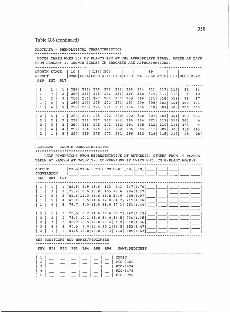
350
Table G.6 (continued)
PLOTDATA - PHENOLOGICAL CHARACTERISTICS ***************************************
NOTES TAKEN WHEN 50% OF PLANTS ARE AT THE APPROPRIATE STAGE. DATES AS DAYS FROM JANUARY 1 . GROWTH SCALES IN BRACKETS ARE APPROXIMATIONS.
GROWTH STAGE | 10 | |( 1 3 ) | ( 3 0 ) | | | | 39 | [ | | |ASPECT |EMRG|LF5A|LF5E|APX1|L10A|L10E| TA j LSLE j ANTH|SILKjMLDSjBLYRj
REP ENT PLT
1 1 1 1 1 1 356 1 264 1 276 1 272 1 282 1 298 1 314 1 321| 317| 319] 31| 34]1 1 3 1 3 1 356 1 263 I 275 1 271| 283 I 296 1 310 1 314] 311| 312 I 4| 10 11 1 3 1 3 1 356| 266| 277 1 272 1 280| 299| 316 1 321| 318 1 319| 16| 17]1 1 5 I 4 11 356] 263 1 2751 270] 280| 293 I 299| 308| 302] 304 I 359] 363 11 1 4 1 5 11 356] 265 1 276] 271| 281| 296 I 304| 310| 307| 308| 359| 363 I
2 1 5 1 1 11 356] 264 1 275| 270 1 280| 292] 300| 307| 303 1 304 1 359 1 363 13 1 3 1 3 11 356] 266 I 277| 272 1 282| 296 I 314] 321| 317| 319| 363 1 4|3 1 3 I 3 11 357] 265| 275| 271| 282 I 294 I 308| 313 1 310| 3111 363 1 4|3 1 4 1 4 11 357] 264 I 276 I 271| 282 1 296 I 305 1 311| 307 I 308] 359| 363 13 1 1 I 5 !1 357] 265| 275 1 272 1 28l| 296 1 312 1 318 1 3151 317] 251 28)
PLOTDATA - GROWTH CHARACTERISTICS *********************************
LEAF DIMENSIONS FROM REPRESENTATIVE AT ANTHESIS. OTHERS FROM 10 PLANTS TAKEN AT RANDOM AT MATURITY. CONVERSIONS IF UNITS NOT: CM;G/PLANT;MG/K;%.
ASPECT IMXLL|MXBL|LFNO|SHWM|GRWT|_KW_|_KN_|CONVERSION I I I I I I I I
REP ENT PLT
J .
1 |82.8| 9 .9 | l 8 .6 l 1 1 3 j 1 4 3 | 3 1 7 | l.7 0 |2 | 7 5 .2 | 1 0 .6 1 1 6 .8 ] 105|77.6| 2 9 4 | l.3 7 |3 1 8 1 .8 1 1 1 .0 il8 .6 | 4 9 .8 | 3 7 .9 | 2 0 9 | l.0 7 |4 |65.1| 9 .6 | l4 .6 | 3 2 .0 | 6 4 .2 l 2 1 5 | l.3 6 |5 |76.7| 9 .0 | 1 5 .0 | 9 1 .9 | 5 7 .3 | 2 6 3 | l.4 4 |
J 1.
5234 1
1 |70.5| 9 .2 | 1 4 .6 | 3 7 .6 | 9 7 .2 | 2 4 2| l.32| _2 | 7 8 .0 | 1 0 .1 | 1 8 .8 1 6 4 .9 1 3 4 .5 1 2 3 0 | l.3 5 |3 I 8 0 .9 | l0 .5 i l7 .0 | 7 7 .4 | 8 1 .2 | 310|l.36|^4 | 8 0 .5 l 9 .0 | 1 5 .4 | 9 0 .1 | 6 4 .5 | 2 5 3 | l .4 7 l '5 | 8 4 .5 | 1 0 .0 | 1 9 .0 | 9 7 .3 | 1 1 2 j 3 0 5 | l.6 3 | '
J I.
KEY POSITIONS AND NAMES/PEDIGREES * * * * * * * * * * * * * * * * * * * * * * * * * * * * * * * * *
KEY RPl RP2 RP3 RP4 RP5 RP6 NAME/PEDIGREE
12345
X304CPIO -3165PIO -3324P IO -3475PIO -3790

351
IBSNAT REDUCED DATA SET FOR MODELLING CROP GROWTH AND DEVELOPMENT PLOTDATA REQUIRED FOR FIELD EXPERIMENTS
Table G.7 Maize data from Kuiaha Experiment Site, natural photoperiod treatment.
GENERAL
PERSONNELRESEARCHER:INSTITUTION:
R ich a rd O gosh i IBSNAT
EXPERIMENT TITLE: ID :
IBSNAT DAYLENGTH/SUMMER;MAIZE 1989 IDSM89K1
TREATMENTSGENOTYPES: 5MANAGEMENT: 1
LOCATIONNAME: KUIAHA
PLOTS** * * *
PLANTING DATE
PLANT DENSITY (PLANTS/M2)
S ep . 8 , 1989
6 .5 7
ORGANISATIONNO.OF ROWS ( # ) : 2ROW LENGTH (M ): 3ROW SPACING (CM ): 75ORIENTATION OF ROWS: E-WALONG OR ACROSS DRAINS: n .a .SPACE BETWEEN PLOTS (CM ): 0GROSS AREA ( M 2 ) : 4 .5
HARVESTNO.OF ROWS: ROW LENGTH (M) AREA ( M 2 ) : METHOD:
121 .5hand
RANDOMIZATION/REPLICATIONDESIGN: RCBNO.OF REPS.-SOWN: 2
-HARVESTED: 2
PROBLEMS********
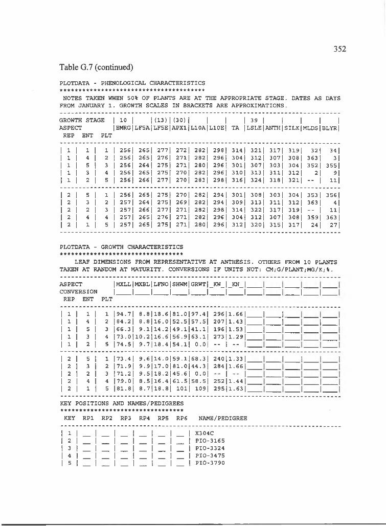
352
Table G.7 (continued)
PLOTDATA - PHENOLOGICAL CHARACTERISTICS ***************************************
NOTES TAKEN WHEN 50% OF PLANTS ARE AT THE APPROPRIATE STAGE. DATES AS DAYS FROM JANUARY 1 . GROWTH SCALES IN BRACKETS ARE APPROXIMATIONS.
GROWTH STAGE | 10 | | (1 3 )| (3 0 )| | | | 39 | | | | |ASPECT |EMRG|LF5A|LF5E|APXllL10AiL10E| TA jLSLEjANTHjSILKjMLDSjBLYR|
REP ENT PLT
1 1 1 1 1 1 256| 265| 277 1 272 1 282 1 298| 3141 3211 3171 3191 321 34 11 1 4 I 2 1 256| 265| 276 I 271| 282 I 296 I 304 1 312 1 3071 308| 363 1 311 1 5 1 3 1 256| 264 1 275 1 2711 280| 296| 3 0 1 1 3071 303 1 304 I 352| 35511 1 3 1 4 1 2561 265 I 275 1 270 1 282| 296| 310 I 313 1 311| 3121 2| 9|1 1 2 1 5 1 256 1 266 1 277 1 270 1 283 I 298| 316| 324 1 318 1 3211 - 1 111
2 1 5 1 1 1 256 1 265| 2751 270 1 2821 294 1 3011 3081 303 1 3041 353 1 356 12 1 3 1 2 1 2571 264 1 275| 269| 282| 294 1 309| 3131 311| 312 I 363 1 4|2 1 2 1 3 1 257| 266 1 2771 2711 2821 298 1 314 I 3221 3171 3191 - 1 1112 1 4 I 4 1 257| 265| 276 1 2711 282| 296 1 304 1 312 1 3071 308| 3591 363 12 1 1 I 5 1 257| 265| 2751 2711 280| 296 I 312| 3201 3151 3171 24 1 271
PLOTDATA - GROWTH CHARACTERISTICS * * * * * * * * * * * * * * * * * * * * * * * * * * * * * * * * *
LEAF DIMENSIONS FROM REPRESENTATIVE AT ANTHESIS. OTHERS FROM 10 PLANTS TAKEN AT RANDOM AT MATURITY. CONVERSIONS IF UNITS NOT: CM;G/PLANT;MG/K;%.
ASPECT CONVERSION
REP ENT
IMXLLIMXBLILFNOISHWMIGRWTI_KW_I_KN_II I I I I I I I J I.
PLT
1 1 1 1 1 194.71 8 . 8 l l 8 . 6 l 8 1 . 0 l 9 7 . 4 l 29611 .6611 1 4 1 2 | 84 .2 l 8 .8 | 1 6 .0 | 5 2 .5 | 5 7 .5 | 2 0 7 l l .4 3 l1 1 5 1 3 166.31 9 .1 | 1 4 .2 | 4 9 .1 | 4 1 .1 | 1 9 6 1 1 .5 3 11 1 3 1 4 | 73 .0 l 1 0 .2 l l6 .6 | 5 6 .9 | 6 3 . l| 2 7 3 l l .2 9 l1 I 2 1 5 | 74 .5 l 9 .7 l l 8 .4 | 5 4 . l | 0 .0 - - 1 - 1
2 1 5 1 1 | 73 .4 l 9 . 6 l l 4 . 0 l 5 9 . l l 6 8 . 3 l 2 4 0 l l .3 3 l2 1 3 1 2 |71.9| 9 .9 | l7 .0 | 8 1 .0 | 4 4 .3 l 2 8 4 l l .6 6 l2 1 2 1 3 171.21 9 .5 | l8 .2 | 4 5 .6 l O .o j - 1 - 1,2 1 4 1 4 179.01 8 .5 | 1 6 .4 | 6 1 .5 | 5 8 .5 | 2 5 2 l l .4 4 l2 1 1 1 5 181.81 8 .7 | l 8 .8 l lO l j 109| 2 9 5 l l .6 3 l
J ____ 1.J ____ I..1____ I.
.1 I
J 1.
J ____ I.J ____ I.
KEY POSITIONS AND NAMES/PEDIGREES * * * * * * * * * * * * * * * * * * * * * * * * * * * * * * * * *
KEY RPl RP2 RP3 RP4 RP5 RP6 NAME/PEDIGREE
12345
X304CPIO -3165PIO -3324PIO -3475PIO -3790
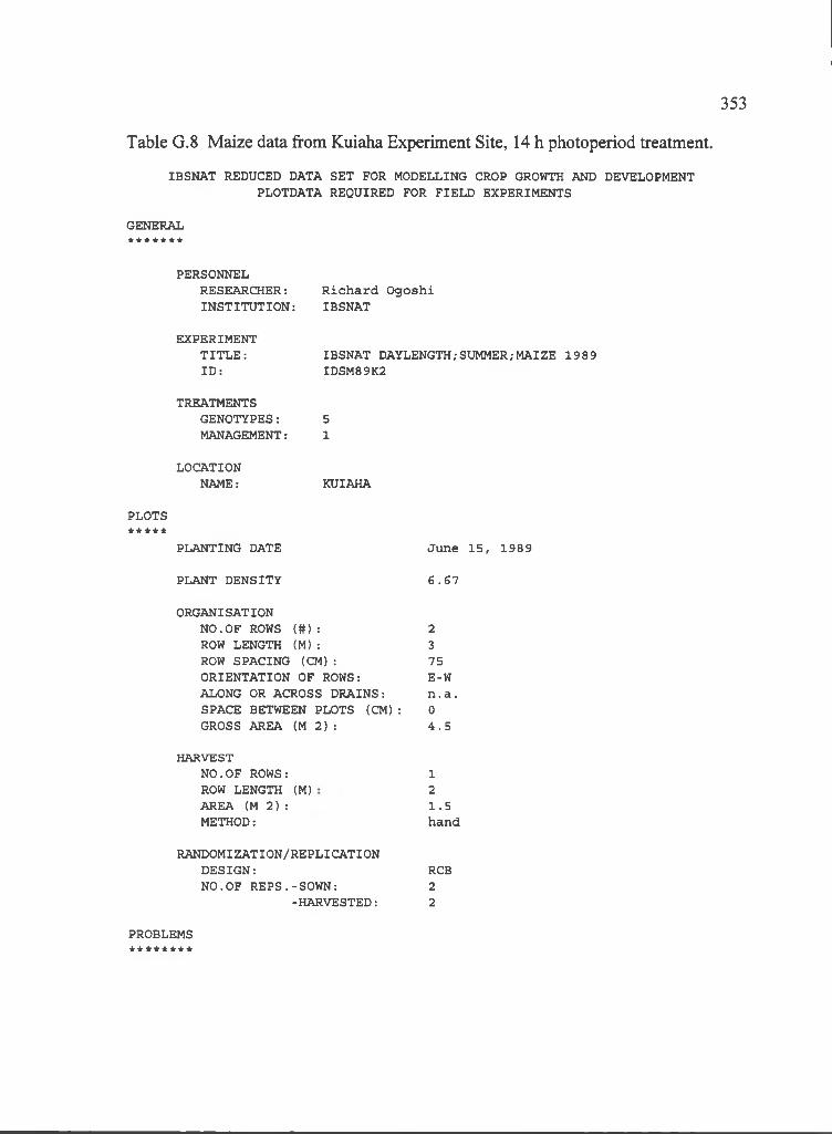
353
IBSNAT REDUCED DATA SET FOR MODELLING CROP GROWTH AND DEVELOPMENT PLOTDATA REQUIRED FOR FIELD EXPERIMENTS
Table G.8 Maize data from Kuiaha Experiment Site, 14 h photoperiod treatment.
GENERAL
PERSONNELRESEARCHER: INSTITUTION:
R ich a rd O gosh i IBSNAT
EXPERIMENT TITLE: ID :
IBSNAT DAYLENGTH/SUMMER;MAIZE 1989 IDSM89K2
TREATMENTSGENOTYPES: 5MANAGEMENT: 1
LOCATIONNAME: KUIAHA
PLOTS* * * * *
PLANTING DATE
PLANT DENSITY
June 15 , 1989
6 .6 7
ORGANISATIONNO.OF ROWS ( # ) : 2ROW LENGTH (M ): 3ROW SPACING (CM ): 75ORIENTATION OF ROWS: E-WALONG OR ACROSS DRAINS: n .a .SPACE BETWEEN PLOTS (CM ): 0GROSS AREA ( M 2 ) : 4 .5
HARVESTNO.OF ROWS: ROW LENGTH (M) AREA ( M 2 ) : METHOD:
121 .5hand
RANDOMIZATION/REPLICATIONDESIGN: RCBNO.OF REPS.-SOWN: 2
-HARVESTED: 2
PROBLEMS********
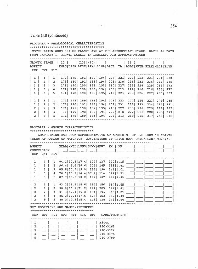
354
Table G.8 (continued)
PLOTDATA - PHENOLOGICAL CHARACTERISTICS ***************************************
NOTES TAKEN WHEN 50% OF PLANTS ARE AT THE APPROPRIATE STAGE. DATES AS DAYS FROM JANUARY 1 . GROWTH SCALES IN BRACKETS ARE APPROXIMATIONS.
GROWTH STAGE j 10 | | ( 1 3 ) 1 ( 3 0 ) | I I I 39 1 1 1 1 1ASPECT 1E M R G |L F5A |L F5E|A PX 1|L10A 1l 1 0E | TA jLSLEjANTH1 SILKjMLDSjBLYRj
REP ENT PLT
1 1 1 4 1 1 1! 1721 179| 1911 1861 194 1 2071 2211 223 1 223 1 223 1 2711 278 11 1 1 1 I 2 1! 173 1 180| 1911 188| 194 I 208| 2301 2351 232 1 2341 296 1 299|1 1 1 2 1 3 11 1711 180 1 190 I 186 I 1951 210 I 2271 2321 228 1 229| 289| 293 11 1 1 5 1 4 11 1711 178 I 190 I 1851 194 I 208 I 213 1 2221 216 1 216 I 268 1 272 11 1 1 3 1 5 11 1711 178 1 190 1 185| 195| 210 I 224 1 2351 226 I 2271 283 I 2871
1 2 1 3 1 1 !1 1711 178 1 1891 1851 1941 2061 223 1 2271 2261 223 1 2791 285|1 2 1 1 I 2 i1 173 1 180| 19l| 188 I 194 I 208 1 231| 2351 233 1 234 1 284 1 2 9 l j1 2 1 2 1 3 11 1711 179| 190| 187| 195| 210] 2271 2351 228 1 229| 289| 292 I1 2 1 4 1 4 11 1711 179 I 190| 185| 1941 209| 218 1 2221 220 I 220| 2751 279|1 2 1 5 I 5 1 1711 178 1 1891 184 I 194 1 206 I 213 1 2191 216 I 2171 2681 272 1
PLOTDATA - GROWTH CHARACTERISTICS *********************************
LEAF DIMENSIONS FROM REPRESENTATIVE AT ANTHESIS. OTHERS FROM 10 PLANTS TAKEN AT RANDOM AT MATURITY. CONVERSIONS IF UNITS NOT: CM,-G/PLANT;MG/K;%.
ASPECTCONVERSION
1MXLL1MXBL1LFNO1SHWM1GRWT1_KW_1_K N _1_J I. .1.
REP ENT PLT
1 1 4 1 1 l 8 4 . l l l 0 .3 | |17.41 127 1 1371 3 0 0 l l . l 5 l1 1 1 I 2 196.4| 9.61 20 .61 202 1 185 1 3 1 8 | l.4 l|1 1 2 1 3 |85.6|10.7| [19 .01 1371 190 I 3 4 l| l .0 l|1 1 5 1 4 | 7 6 .l l l 0 .9 | |14.41 87 .21 114 I 3 2 4 | l.5 l|1 1 3 1 5 | 8 7 .7 | 1 0 .3 1 1 8 .2l 1571 1371 3 5 7 11 . 4 1 1
2 1 3 1 1 l 8 3 . 2 l l l . 6 | 118.61 152 1 156 1 3 6 7 l l .6 5 l3 1 1 I 2 l 9 8 . 6 l l 0 . 7121 .21 224 I 203 1 3 4 4 | l.4 l|2 1 2 I 3 l 9 1 . 3 l l 2 . l | 119.21 194 I 194 1 3 4 0 | l .0 l l2 I 4 1 4 | 8 5 .2 | 1 0 .4 |17.61 123 1 153 1 3 3 0 ll .3 0 |2 1 5 1 5 1 8 0 .o l i o . 8 l l 5 . 4 l 118 1 130 1 343 11 .6 6 I
.1____ I.
.1____ I.
J I.J ____IJ ____I
KEY POSITIONS AND NAMES/PEDIGREES * * * * * * * * * * * * * * * * * * * * * * * * * * * * * * * * *
KEY RPl RP2 RP3 RP4 RP5 RP6 NAME/PEDIGREE
X304CP IO -3165PIO -3324PIO -3475PIO -3790

355
IBSNAT REDUCED DATA SET FOR MODELLING CROP GROWTH AND DEVELOPMENT PLOTDATA REQUIRED FOR FIELD EXPERIMENTS
Table G.9 Maize data from Kuiaha Experiment Site, 17 h photoperiod treatment.
GENERAL
PERSONNELRESEARCHER:INSTITUTION:
R ich a rd O gosh i IBSNAT
EXPERIMENT TITLE: ID :
IBSNAT DAYLENGTH/SUMMER;MAIZE 1989 IDSM89K3
TREATMENTSGENOTYPES: 5MANAGEMENT: 1
LOCATIONNAME: KUIAHA
PLOTS* * * * *
PLANTING DATE
PLANT DENSITY (PLANTS/M2)
June 1 5 , 1989
6 .67
ORGANISATIONNO.OF ROWS ( # ) : 2ROW LENGTH (M ): 3ROW SPACING (CM ): 75ORIENTATION OF ROWS: E-WALONG OR ACROSS DRAINS: n .a .SPACE BETWEEN PLOTS (CM ): 0GROSS AREA ( M 2 ) : 4 .5
HARVESTNO.OF ROWS: ROW LENGTH (M) AREA (M 2 ) : METHOD:
121 .5hand
RANDOMIZATION/REPLICATIONDESIGN: RCBNO.OF REPS.-SOWN: 2
-HARVESTED: 2
PROBLEMS********
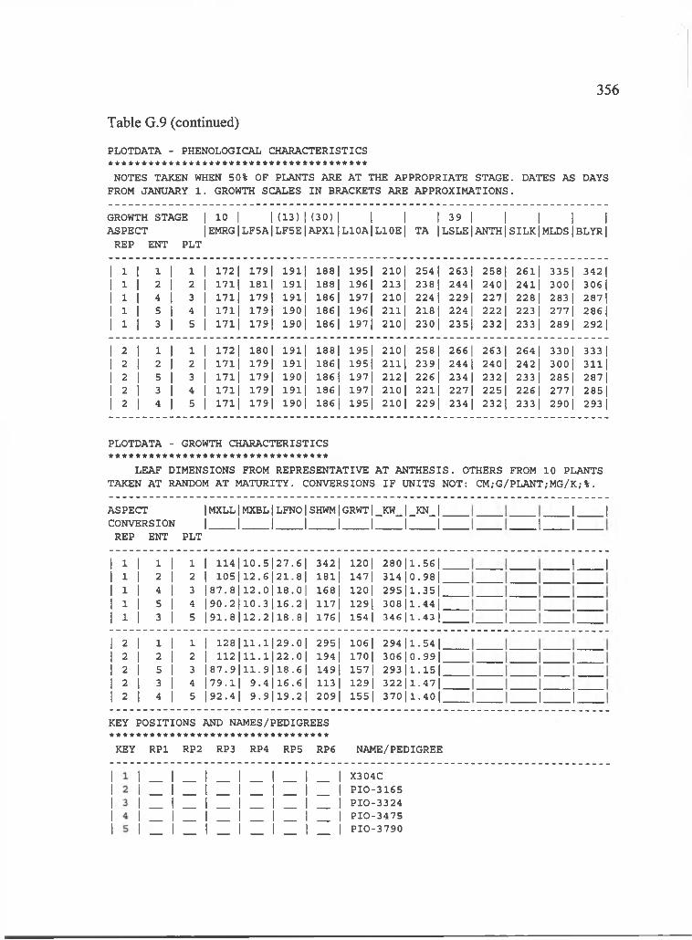
356
PLOTDATA - PHENOLOGICAL CHARACTERISTICS
NOTES TAKEN WHEN 50% OF PLANTS ARE AT THE APPROPRIATE STAGE. DATES AS DAYS FROM JANUARY 1 . GROWTH SCALES IN BRACKETS ARE APPROXIMATIONS.
GROWTH STAGE | 10 | 1 (1 3 )| (3 0 )| [ | | 39 | | | [ |ASPECT |EMRG|LF5A|LF5E|APXllL10A|L10E| TA |LSLE|ANTHjSILKjMLDSjBLYR|
REP ENT PLT
Table G.9 (continued)
1 1 1 1 1 11 172 1 179| 191| 188 1 195| 210 1 254 1 263 1 258 1 2611 3351 342 11 1 2 I 2 11 1711 I S l j 19l| 188 I 196 I 213 1 238 I 244 I 240 1 24l| 3001 306|1 1 4 1 3 11 1711 179] 191| 186| 197 I 210 1 224 1 229| 227 1 228 I 283 I 287]1 1 5 I 4 11 1711 179| 190 I 186| 196 1 21l| 218| 224 I 222 1 223 1 277| 286 I1 1 3 1 5 11 1711 179 I 190 1 186| 197| 210| 230| 2351 232 1 233 1 2891 292 I
2 1 1 1 1 11 172 1 180 1 1911 188| 1951 210| 258| 2661 263 1 264 1 3301 33312 1 2 1 2 11 1711 179 I 1911 186 1 195| 211| 239| 244 1 240| 242 I 300| 311|3 1 5 1 3 11 1711 179 I 190 I 186 I 197| 212 1 226 I 234 1 232 1 233 1 285 I 28712 I 3 1 4 11 1711 179| 19l| 186 I 197| 210 1 221| 227| 2251 226 1 2771 285|2 1 4 1 5 11 1711 179 I 190 1 186 I 195| 210 I 229| 234| 232| 233 1 290 1 293 1
PLOTDATA - GROWTH CHARACTERISTICS *********************************
LEAF DIMENSIONS FROM REPRESENTATIVE AT ANTHESIS. OTHERS FROM 10 PLANTS TAKEN AT RANDOM AT MATURITY. CONVERSIONS IF UNITS NOT: CM;G/PLANT;MG/K;%.
ASPECT CONVERSION
REP ENT
IMXLLIMXBLILFNOISHWMIGRWTI_KW_I_KN_II I I I 1 I I I
PLT.1 I.
.1 I
1 1 1 1 1 1 1 1 4 l l 0 .5 l 2 7 .6 l 3421 120 1 280 | l.5 6 l1 1 3 1 2 1 1 05| 12 .6| 21 .8| 18l| 147 I 314 10.9811 1 4 1 3 | 8 7 .8 | 1 2 .0 | 1 8 .0 | 168| 120| 295 11.3511 1 5 I 4 | 9 0 .2 t l 0 .3 l l 6 . 2 l 1171 1291 308 | l.4 4 l1 1 3 I 5 | 9 1 .8 l l 2 .2 l l 8 .8 | 1761 154 1 346 | l .4 3 l
3 1 1 1 1 1 1 2 8 l l l . l l 2 9 . 0 l 2951 1061 294 | l .5 4 l3 1 3 1 2 I 1 12| 11 .1| 22 .0| 194 I 170| 306 10.9913 1 5 1 3 | 8 7 .9 | 1 1 .9 | 1 8 .6 | 149| 1571 293 11.1513 1 3 1 4 |79.1| 9 .4 | 1 6 .6 | 113 1 1291 3 2 2 l l .4 7 l3 1 4 1 5 |92.4| 9 .9 | 1 9 .2 | 2091 1551 3 7 0 l l .4 0 l
.1 I
J I.
KEY POSITIONS AND NAMES/PEDIGREES * * * * * * * * * * * * * * * * * * * * * * * * * * * * * * * * *
KEY RPl RP2 RP3 RP4 RP5 RP6 NAME/PEDIGREE
X304CPIO -3165PIO -3324PIO -3475PIO -3790

357
IBSNAT REDUCED DATA SET FOR MODELLING CROP GROWTH AND DEVELOPMENT PLOTDATA REQUIRED FOR FIELD EXPERIMENTS
Table G.IO Maize data from Kuiaha Experiment Site, 20 h photoperiod treatment.
GENERAL
PERSONNELRESEARCHER:INSTITUTION:
R ich a rd O gosh i IBSNAT
EXPERIMENT TITLE: ID :
IBSNAT DAYLENGTH/SUMMER;MAIZE 1989 IDSM89K4
TREATMENTSGENOTYPES: 5MANAGEMENT: 1
LOCATIONNAME: KUIAHA
PLOTS* * * * *
PLANTING DATE
PLANT DENSITY (PLANT/M2)
June 15 , 1989
6 .6 7
ORGANISATIONNO.OF ROWS ( # ) : 2ROW LENGTH (M ): 3ROW SPACING (CM ): 75ORIENTATION OF ROWS: E-WALONG OR ACROSS DRAINS: n .a .SPACE BETWEEN PLOTS (CM): 0GROSS AREA ( M 2 ) : 4 .5
HARVESTNO.OF ROWS: ROW LENGTH (M) AREA ( M 2 ) : METHOD:
121 .5hand
RANDOMIZATION/REPLICATIONDESIGN: RCBNO.OF REPS.-SOWN: 2
-HARVESTED: 2
PROBLEMS

358
PLOTDATA - PHENOLOGICAL CHARACTERISTICS
Table G.IO (continued)
NOTES TAKEN WHEN 50% OF PLANTS ARE AT THE APPROPRIATE STAGE. DATES AS DAYS FROM JANUARY 1 . GROWTH SCALES IN BRACKETS ARE APPROXIMATIONS.
GROWTH STAGE | 10 | |( 1 3 ) | ( 3 0 ) \ \ \ 1 39 | ] | | |ASPECT |EMRGlLF5A|LF5ElAPXl|L10A|L10E| TA |LSLEjANTH|SILKjMLDSjBLYR|
REP ENT PLT
1 1 1 3 1 1 I 1711 179 1 189| 186 1 196 1 2101 2301 2341 2321 234 1 290 1 293 11 1 1 4 1 2 1 171| 179| 192 I 187| 198 j 213 1 2271 234| 2311 233 1 290 I 293 11 1 1 3 1 3 1 1711 180| 191| 188 I 196 1 2111 2371 244 I 2391 24l| 310 I 31311 1 1 1 I 4 1I 172 1 179| 191| 188| 195| 210 1 2571 267| 263 1 277| 3351 343 11 1 1 5 I 5 11 1711 179| 190| 186 1 195 1 210 I 2211 2251 223 1 225 1 276 1 285|
1 3 1 5 1 1 11 1711 179 1 190 1 186 1 197 1 2101 2221 2271 224 1 2261 276 1 28011 2 1 3 1 2 11 1711 179 I 190| 186 1 195| 210 1 231| 2361 233 1 234 1 290] 294 I1 2 1 4 1 3 11 1711 179| 19l| 186 I 195| 210| 2271 234 I 2311 233 1 286 1 287|1 2 I 1 I 4 11 1721 179| 1911 188| 194 I 210| 258 1 2671 264 1 2791 3351 342 I1 2 1 2 1 5 11 1711 180| 191| 1861 196 1 2111 242 I 2511 244 I 248] 304 1 307|
PLOTDATA - GROWTH CHARACTERISTICS
LEAF DIMENSIONS FROM REPRESENTATIVE AT ANTHESIS. OTHERS FROM 10 PLANTS TAKEN AT RANDOM AT MATURITY. CONVERSIONS IF UNITS NOT: CM;G/PLANT;MG/K;%.
ASPECT I_MXLL 1 MXBL I LFNO I SHWM I GRWT I _KW_ I _KN_ I______|______|______|______|______|CONVERSION______I I 1 I I I I I______I______I______I______I______I
REP ENT PLT
1 | 9 2 .3 | 1 2 .4 | 1 9 .2 |2 1 9 0 .6 | 1 2 .6 | 1 8 .6 |3 1 105 I 1 2 .0 I 2 2 .0 I4 I 119| 9 .1 | 2 6 .2 |5 | 8 1 .6 | 1 0 .4 | 1 6 .6 {
176| 134| 344|1.51|_ 183| 1441 3 0 3 | 1 .2 8 | ' 212| 156| 3 0 8 | 1 .2 5 L 853|60.0| 374|2.02|^l io j 112| 30oil.54|^
1 | 8 4 .6 | 1 0 .0 | 1 6 .6 | 125| 127| 2 9 4 | l.5 3 | .2 | 9 5 .2 | 1 2 .4 | 1 9 .2 | 1 6 6 j 168| 3 6 3 | l.4 0 | '3 | 9 4 .6 | 1 1 .9 | 1 9 .4 | 1 8 0 j 1 6 6 j 3 1 l| l.2 8 | ^4 I 113| 9 .8 | 2 9 .6 | 584|50.9| 357|l.88|^5 I 1 1 3 | 1 3 .2| 22 .0| 182| 117| 276|l.25|^
KEY POSITIONS AND NAMES/PEDIGREES *********************************
KEY RPl RP2 RP3 RP4 RP5 RP6 NAME/PEDIGREE
X304CPIO -3165PIO -3324PIO -3475PIO -3790

359
APPENDIX H Maize data, summer 1990
Table H.l Maize data from Haleakala Experiment Station, control photoperiod treatment.
IBSNAT REDUCED DATA SET FOR MODELLING CROP GROWTH AND DEVELOPMENT PLOTDATA REQUIRED FOR FIELD EXPERIMENTS
GENERAL
PERSONNELRESEARCHER; INSTITUTION:
R ich a rd O gosh i IBSNAT
EXPERIMENT TITLE: ID :
IBSNAT DAYLENGTH/SUMMER;MAIZE 1990 IDSM90H0
TREATMENTSGENOTYPES: 5MANAGEMENT: 0
LOCATIONNAME: H a le a k a la E xperim en t S t a t io n
PLOTS* * * * *
PLANTING DATE May 1 7 , 1990
PLANTING DENSITY ( PLANTS/M2) 6 .6 7
ORGANISATIONNO.OF ROWS ( # ) : 2ROW LENGTH (M ): 3ROW SPACING (CM ): 75ORIENTATION OF ROWS: E-WALONG OR ACROSS DRAINS: n .a .SPACE BETWEEN PLOTS (CM ): 0GROSS AREA ( M 2 ) : 4 .5
HARVESTNO.OF ROWS: ROW LENGTH (M) AREA (M 2 ) : METHOD:
121 .5hand
RANDOM IZATI ON/RE PL I CAT I ONDESIGN: RCBNO.OF REPS.-SOWN: 2
-HARVESTED: 2
PROBLEMS********
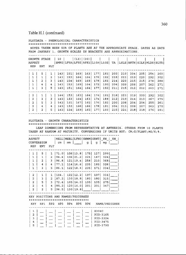
360
PLOTDATA - PHENOLOGICAL CHARACTERISTICS
Table H.l (continued)
NOTES TAKEN WHEN 50% OF PLANTS ARE AT THE APPROPRIATE STAGE. DATES AS DAYS FROM JANUARY 1 . GROWTH SCALES IN BRACKETS ARE APPROXIMATIONS.
GROWTH STAGE | 10 | |( 1 3 ) |( 3 0 ) | | | | | | | | |ASPECT |EMRG|LF5A|LF5E|APX1|L10A|L10E| TA jLSLEjANTH|SILKjMLDSjBLYRj
REP ENT PLT
1 1 5 1 1 1 143 1 1511 1691 163 1 1771 193 1 2001 2101 204 1 205 1 254 1 260 11 1 1 1 2 1 143 1 153 1 164 1 164 1 176 1 1921 218 1 223 1 219| 220 j 292 I 302 11 1 2 I 3 11 143 1 154 1 169| 168 I 178 I 193 1 214 1 220 1 215| 2151 278 I 288 11 1 4 I 4 11 143 1 153 1 169| 164 I 172 I 190| 204 I 209| 2081 2071 262| 27111 1 3 1 5 11 143 1 1511 164 I 164 I 177 1 192 I 2111 215 I 212 I 212 1 263 1 2711
2 1 1 1 1 11 144 1 153 1 163 1 164 1 174 1 1911 218 1 223 1 2191 220 1 292| 302 12 I 3 1 2 11 143 1 153 1 164 I 163 1 174 I 189| 212 1 2191 214 I 213 1 267 1 27512 1 5 1 3 11 143 1 1511 167| 165| 176 I 192 I 2001 208| 204 I 204 1 255 1 26112 1 4 1 4 11 143 1 153 1 166 1 166 1 178 I 1911 204 I 213 1 208 I 207| 263 1 270|2 I 2 1 5 i1 143 1 154 1 169| 165| 1771 193 1 2151 2211 218 1 218 I 276 I 281|
PLOTDATA - GROWTH CHARACTERISTICS *********************************LEAF DIMENSIONS FROM REPRESENTATIVE AT ANTHESIS’ OTHERS FROM 10 PLANTS
TAKEN AT RANDOM AT MATURITY. CONVERSIONS IF UNITS NOT: CM;G/PLANT;MG/K;%.
AS PECT IMXLL|MXBL|LFNO|SHWM|GRWT|_KW_|_KN_|CONVERSION I cm I mm j j g [ g j mg | j
REP ENT PLT
5 1 1 | 71 .0 l 106 113.81 1751 1271 29911 I 2 194.41 106 121.21 3211 187| 324 I2 1 3 196.81 121 |19.41 2581 210| 368 I4 1 4 | 7 7 .l l 114 116.61 2351 185| 326|3 1 5 1 8 6 .l l 122 118.41 2351 1711 334|
2 1 1 1 1 1104.1 122 112.21 1971 1971 33112 I 3 1 2 187.21 130 118.81 180| 18oj 31512 1 5 1 3 | 72 .4 l 105 114.01 1351 1351 27512 1 4 1 4 185.21 1 2 0 1 1 6 .Ol 2011 2011 347|2 1 2 1 5 | 96 .5 l 130|19.8| 1 1 1
KEY POSITIONS AND NAMES/PEDIGREES *********************************
KEY RPl RP2 RP3 RP4 RP5 RP6 NAME/PEDIGREE
12345
X304CPIO -3165PIO -3324P IO -3475P IO -3790

361
IBSNAT REDUCED DATA SET FOR MODELLING CROP GROWTH AND DEVELOPMENT PLOTDATA REQUIRED FOR FIELD EXPERIMENTS
GENERAL
Table H.2 Maize data from Haleakala Experiment Station, natural photoperiodtreatment.
PERSONNELRESEARCHER:INSTITUTION:
R ich a rd O gosh i IBSNAT
EXPERIMENT TITLE: ID :
IBSNAT DAYLENGTH;SUMMER;MAIZE 1990 IDSM90H1
TREATMENTSGENOTYPES: 5MANAGEMENT: 0
LOCATIONNAME: H a lea k a la E xperim ent S t a t io n
PLOTS*****PLANTING DATE
PLANT DENSITY (PLANTS/M2)
May 17 , 1990
6 .6 7
ORGANISATIONNO.OF ROWS ( # ) : 2ROW LENGTH (M ): 3ROW SPACING (CM ): 75ORIENTATION OF ROWS: E-WALONG OR ACROSS DRAINS: n .a .SPACE BETWEEN PLOTS (CM): 0GROSS AREA ( M 2 ) : 4 .5
HARVESTNO.OF ROWS: ROW LENGTH (M) AREA (M 2 ) : METHOD:
121 .5hand
RANDOMIZATION/REPLICATIONDESIGN: RCBNO.OF REPS.-SOWN: 2
-HARVESTED: 2
PROBLEMS********
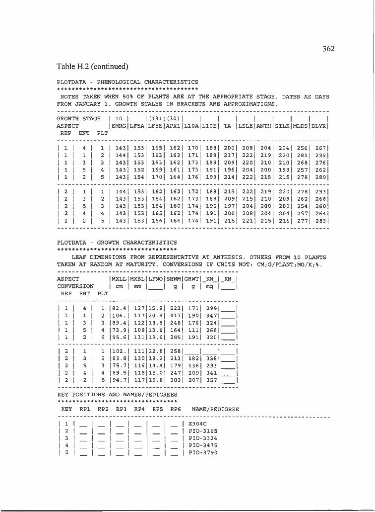
362
PLOTDATA - PHENOLOGICAL CHARACTERISTICS
Table H.2 (continued)
NOTES TAKEN WHEN 50% OF PLANTS ARE AT THE APPROPRIATE STAGE. DATES AS DAYS FROM JANUARY 1 . GROWTH SCALES IN BRACKETS ARE APPROXIMATIONS.
GROWTH STAGE | 10 | 1 (1 3 )1 (3 0 )| I I I I I I I IASPECT |EMRG|LF5A|LF5E|APX1|L10A|L10E| TA jLSLE[ANTHjSILK|MLDS|BLYRj
REP ENT PLT
1 1 1 4 1 1 1 143 1 153 1 165| 162 1 170 1 1881 2001 2081 204 1 204 1 256 1 26711 1 1 1 I 2 1 144 1 153 1 163 I 163 I 1711 188 I 217| 222 1 219| 220 1 2 8 1 1 299|1 1 1 3 1 3 1 143 1 153 1 163 I 162 I 173 1 189| 2091 2201 210| 210 I 268 I 276 I1 1 1 5 1 4 11 143 1 152 1 169| 161| 173 1 1 9 l j 196 I 204 I 200| 199| 257| 262|1 1 1 2 1 5 11 143 1 154 I 170 I 164 1 176'| 193 1 214 I 222| 2151 2151 278 1 289|
1 2 1 1 1 1 11 144 1 153 1 1621 1621 172 1 188 1 2151 222 1 2191 2201 2781 293 11 2 1 3 1 2 11 143 1 153 1 164 I 162 1 173 1 188 I 209| 2151 210| 209| 262| 268|I 2 1 5 1 3 11 143 1 1531 164 I 160 I 174 1 190| 197| 204 1 200| 200 I 254 I 260|1 2 1 4 1 4 11 143 1 153 1 165| 162 1 174 I 1 9 1 1 200| 208| 204 I 204 I 257] 264 I1 2 I 2 1 5 11 143 1 153 1 166 I 166 I 174 1 19l| 215| 2211 215| 216 I 277 1 283 I
PLOTDATA - GROWTH CHARACTERISTICS * * * * * * * * * * * * * * * * * * * * * * * * * * * * * * * * *
LEAF DIMENSIONS FROM REPRESENTATIVE AT ANTHESIS. OTHERS FROM 10 PLANTS TAKEN AT RANDOM AT MATURITY. CONVERSIONS IF UNITS NOT: CM,-G/PLANT,-MG/K;%.
ASPECT IMXLL|MXBL|LFNO|SHWM|GRWT|_KW_ j _KN_|CONVERSION I cm I mm j j g | g | mg | j
REP ENT PLT
1 1 1 4 1 1 | 82 .4 l 127115 .81 223 1 171| 2991 11 1 1 1 I 2 1106.1 1171 20.81 417 I 1901 347| 11 1 1 3 1 3 189.41 1221 1 8 .8| 248| 176 I 324| 11 1 1 5 1 4 | 73 .9 l 1091 1 3 .6| 164 I 111| 268 1 11 1 1 3 1 5 | 95 .6 l 131| 1 9 .6| 285 1 1911 3201 1
1 3 1 1 1 1 |102. 1 111| 2 2 .8 1 258 1 1 1 11 2 1 3 I 2 183.81 1301 1 8 .2| 213 1 1821 3381, 11 2 1 5 1 3 | 75 .7 l 116 I1 4 .4 I 179 1 136 I 2931, 11 2 1 4 1 4 | 89 .5 l 118| 1 5 .0| 247| 209| 3411 1I 2 I 2 I 5 |94.7| 1 1 7 | l9 .8 l 303 I 207 1 3571 1
KEY POSITIONS AND NAMES/PEDIGREES * * * * * * * * * * * * * * * * * * * * * * * * * * * * * * * * *
KEY RPl RP2 RP3 RP4 RP5 RP6 NAME/PEDIGREE
12345
X304CPIO -3165PIO -3324PIO -3475PIO -3790
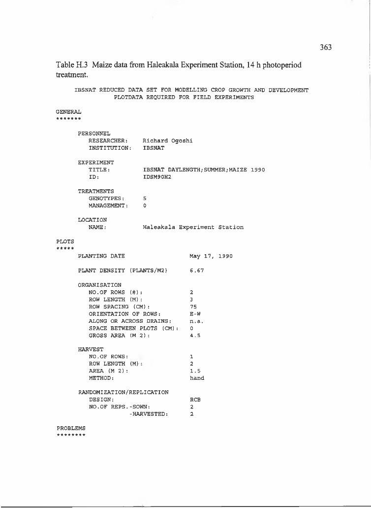
363
IBSNAT REDUCED DATA SET FOR MODELLING CROP GROWTH AND DEVELOPMENT PLOTDATA REQUIRED FOR FIELD EXPERIMENTS
GENERAL
Table H.3 Maize data from Haleakala Experiment Station, 14 h photoperiodtreatment.
PERSONNELRESEARCHER:INSTITUTION:
R ich a rd O gosh i IBSNAT
EXPERIMENT TITLE: ID :
IBSNAT DAYLENGTH/SUMMER;MAIZE 1990 IDSM90H2
TREATMENTSGENOTYPES: 5MANAGEMENT: 0
LOCATIONNAME: H a le a k a la E xperim ent S t a t i o n
PLOTS* * * * *
PLANTING DATE
PLANT DENSITY (PLANTS/M2)
May 17 , 1990
6 .6 7
ORGANISATIONNO.OF ROWS ( # ) : 2ROW LENGTH (M ): 3ROW SPACING (CM ): 75ORIENTATION OF ROWS: E-WALONG OR ACROSS DRAINS: n .a .SPACE BETWEEN PLOTS (CM ): 0GROSS AREA ( M 2 ) : 4 .5
HARVESTNO.OF ROWS: ROW LENGTH (M) AREA ( M 2 ) : METHOD:
121 .5hand
RANDOMIZATION/REPLICATIONDESIGN: RCBNO.OF REPS.-SOWN: 2
-HARVESTED: 2
PROBLEMSIt * * -k * * * *
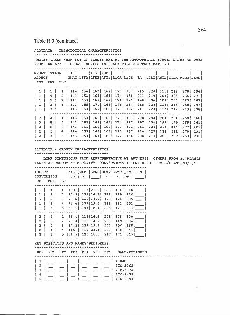
364
Table H.3 (continued)
PLOTDATA - PHENOLOGICAL CHARACTERISTICS ***************************************
NOTES TAKEN WHEN 50% OF PLANTS ARE AT THE APPROPRIATE STAGE. DATES AS DAYS FROM JANUARY 1 . GROWTH SCALES IN BRACKETS ARE APPROXIMATIONS.
GROWTH STAGE | 10 | | ( 1 3 ) | ( 3 0 ) | | | | | | | | |ASPECT |E M R G |L F 5A |L F 5E |A P X 1|L 10A |L 10E | TA jLSLE|ANTH |SILK jM LDSjBLYR]
REP ENT PLT
1 1 1 1 1 1 1 144 1 154 1 162] 162] 170] 187] 215] 220] 216 1 218] 278 1 296]1 1 1 4 1 2 1I 143 1 153 1 166 1 164 I 174 I 188 1 203 1 210| 204 I 205) 264 1 271]1 1 1 5 I 3 1i 143 1 153 1 169| 162 I 174 I 1 9 1 1 198) 206 I 204 I 204| 260) 267]1 1 1 3 1 4 11 143 1 1551 171| 169| 176 1 194 I 215 1 228 I 216 I 218] 288 I 297|1 1 1 3 1 5 11 143 1 153 1 166) 166 I 173] 192 I 211) 220 I 213] 212) 269) 278 1
1 3 1 4 1 1 11 143 1 153 1 165] 162 1 173] 187] 200] 208] 204 1 204 1 260 1 268 11 3 1 5 1 2 11 143 1 153 1 164 I 1 6 1 1 174 1 187| 197 I 204 I 199) 199| 255] 26111 3 1 2 I 3 11 143 1 155 1 169| 166| 173] 192| 211] 220) 213] 214 I 277] 2 8 l j1 3 I 1 I 4 11 144 1 153] 162 I 163 1 170] 187] 218] 227] 222] 221| 278] 29111 3 1 3 1 5 11 143 1 153 1 163 1 162 1 172] 188 I 208 I 214 1 209] 209| 263 I 278|
PLOTDATA - GROWTH CHARACTERISTICS * * * * * * * * * * * * * * * * * * * * * * * * * * * * * * * * *
LEAF DIMENSIONS FROM REPRESENTATIVE AT ANTHESIS. OTHERS FROM 10 PLANTS TAKEN AT RANDOM AT MATURITY. CONVERSIONS IF UNITS NOT: CM;G/PLANT;MG/K;%.
ASPECT ]MXLL] MXBL] LFNO] SHWM] GRWT)__KW_1_KN_1CONVERSION 1 cm 1 mm 1 1 g I g 1 mg 1 I
REP ENT PLT
1 1 1 1 1 1 |110.| 118 12 1 .2 ] 289) 184] 318] 11 1 1 4 1 2 ]8 0 .9 l 124 11 6 .2 ] 233] 189| 316| 11 1 1 5 I 3 173.51 n i l 1 4 .0 ] 178] 125] 385] 11 1 1 3 1 4 | 96 .4 ) 133 1|19.8| 311] 211] 352] 11 1 1 3 I 5 1 8 6 .4 ] 143 1|18.41 223 1 173 1 3331 1
1 3 1 4 1 1 ]8 6 .4 ] 119 1|16.8] 208 1 178 1 300] 11 3 1 5 1 2 | 73 .0 ] 120 |14.2] 209| 149| 304) 11 2 I 3 1 3 ]8 7 .2 ] 129 |19.4| 274 I 196 1 3651 11 3 1 1 I 4 ] 1 0 6 . 1 119 |33.4] 293] 180 1 341| 11 3 1 3 1 5 1 8 6 .5 ] 120 |18.0) 217] 171] 313 1 1
KEY POSITIONS AND NAMES/PEDIGREES * * * * * * * * * * * * * * * * * * * * * * * * * * * * * * * * *
KEY RPl RP2 RP3 RP4 RP5 RP6 NAME/PEDIGREE
X304CPIO -3165PIO -3324PIO -3475PIO -3790
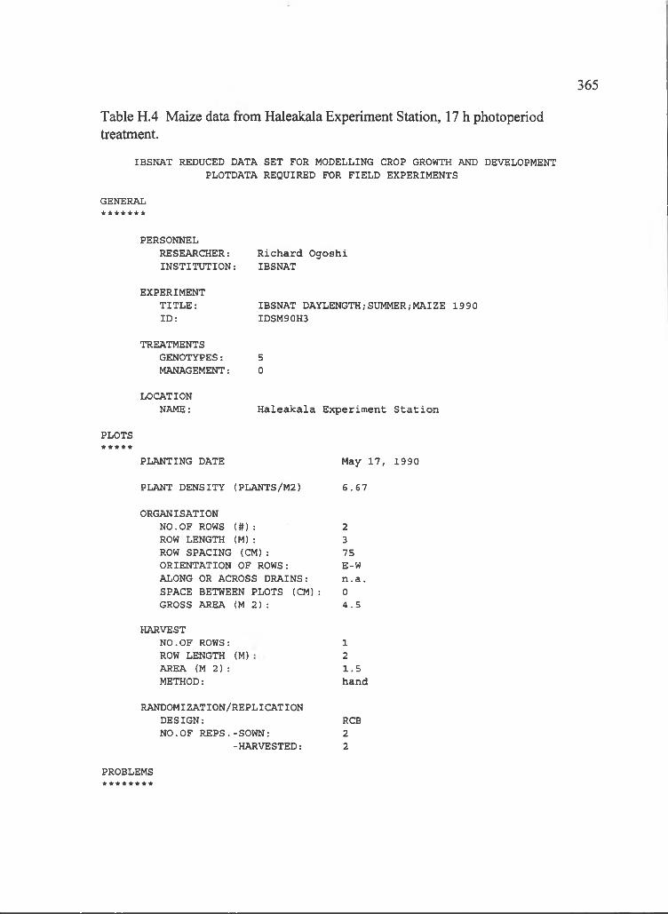
365
IBSNAT REDUCED DATA SET FOR MODELLING CROP GROWTH AND DEVELOPMENT PLOTDATA REQUIRED FOR FIELD EXPERIMENTS
GENERAL
Table H.4 Maize data from Haleakala Experiment Station, 17 h photoperiodtreatment.
PERSONNELRESEARCHER: INSTITUTION:
R ich a rd O gosh i IBSNAT
EXPERIMENT TITLE: ID :
IBSNAT DAYLENGTH;SUMMER;MAIZE 1990 IDSM90H3
TREATMENTSGENOTYPES: 5MANAGEMENT: 0
LOCATIONNAME: H a le a k a la E xperim ent S t a t i o n
PLOTS* * * * *
PLANTING DATE
PLANT DENSITY (PLANTS/M2)
May 17 , 1990
6 .6 7
ORGANISATIONNO.OF ROWS ( # ) : 2ROW LENGTH (M ): 3ROW SPACING (CM ): 75ORIENTATION OF ROWS: E-WALONG OR ACROSS DRAINS: n .a .SPACE BETWEEN PLOTS (CM ): 0GROSS AREA ( M 2 ) : 4 .5
HARVESTNO.OF ROWS: ROW LENGTH (M) AREA ( M 2 ) : METHOD:
121 .5hand
RANDOMIZATION/REPLICATIONDESIGN: RCBNO.OF REPS.-SOWN: 2
-HARVESTED: 2
PROBLEMS********
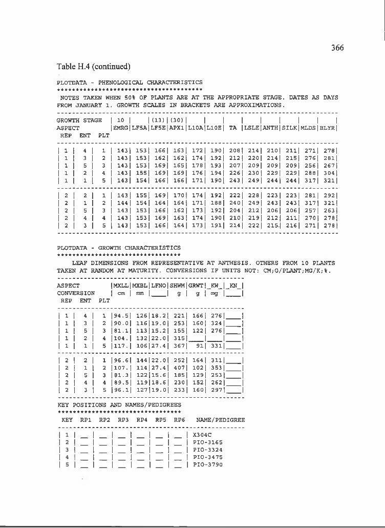
366
Table H.4 (continued)
PLOTDATA - PHENOLOGICAL CHARACTERISTICS ***************************************NOTES TAKEN WHEN 50% OF PLANTS ARE AT THE APPROPRIATE STAGE. DATES AS DAYS
FROM JANUARY 1 . GROWTH SCALES IN BRACKETS ARE APPROXIMATIONS.
GROWTH STAGE | 10 | | (1 3 )| (3 0 )| I I I I I I I IASPECT |EMRG|LF5A|LF5E|APX1|L10A1l 10E| TA jLSLEjANTHjSILK|MLDSjBLYRj
REP ENT PLT
1 1 4 1 1 1 143 1 153 1 166 1 163 1 172 1 190 1 2081 214 1 210 1 2111 2711 278 11 1 3 I 2 1 143 1 153 1 162 I 162 1 174 1 192 1 212| 220 I 214 1 215| 276 1 28l|1 1 5 I 3 1 143 1 153 1 169| 165 1 178 I 193 1 207| 209| 209| 209| 256 1 267|1 1 2 1 4 1 143 1 1551 169| 169| 176 I 194 1 226 1 230 1 229 I 229| 288 I 304 11 1 1 1 5 11 143 1 154 1 166 I 166 I 1711 1901 243 1 249| 244 1 244 I 3171 3211
2 1 2 1 1 11 143 1 155 1 1691 1701 174 1 192 1 222 1 228 1 223 1 223 1 2811 292 12 I 1 I 2 11 144 1 154 1 164 I 164 1 1711 188 1 240| 2491 243 1 243 1 3171 32112 1 5 I 3 11 143 1 153 1 166 I 162 1 173 1 192 I 204 1 212 1 206| 206| 2571 263 12 1 4 1 4 !1 143 1 153 1 169| 163 I 174 1 190 I 210 I 2191 212 I 2111 270| 278|2 1 3 1 5 11 143 1 153 1 166 I 164 I 173 1 191| 214 I 222 I 215.1 216 1 2711 2781
PLOTDATA - GROWTH CHARACTERISTICS
LEAF DIMENSIONS FROM REPRESENTATIVE AT ANTHESIS. OTHERS FROM 10 PLANTS TAKEN AT RANDOM AT MATURITY. CONVERSIONS IF UNITS NOT: CM;G/PLANT;MG/K;%.
ASPECT CONVERSION
REP ENT
IMXLLIMXBL|LFNO|SHWM|GRWT|_KW_|_KN_| I cm I mm j j g j g | mg j j
PLT
1 1 1 4 1 1 | 9 4 .5 l 126 118.21 2211 166 1 276 1 11 1 1 3 1 2 190.01 116 119.01 253 1 160 1 324 1 11 1 1 5 I 3 |81.1| 113 115.21 1551 122 1 276| 11 1 1 2 I 4 1104.1 132 122.01 315| 1 1 11 1 1 1 I 5 1117.1 106 | 27 .4 l 3671 911 3311 1
1 2 1 2 1 1 196.61 144 122.01 252 1 164 1 311| 1I 2 1 1 1 2 1107.1 114 | 27 .4 l 407| 102 I 3531 11 2 1 5 1 3 | 81 .3 l 122 |15.6| 185| 1291 253 1 11 2 1 4 1 4 | 89 .5 l 1 1 9 1 1 8 .6l 2301 152 1 262 1 11 2 1 3 1 5 |96.1| 127 |19.0| 233 1 160l 2971 1
KEY POSITIONS AND NAMES/PEDIGREES * * * * * * * * * * * * * * * * * * * * * * * * * * * * * * * * *
KEY RPl RP2 RP3 RP4 RP5 RP6 NAME/PEDIGREE
1 X304C I P IO -3165 I PIO -3324 I PIO -3475 I PIO -3790

367
IBSNAT REDUCED DATA SET FOR MODELLING CROP GROWTH AND DEVELOPMENT PLOTDATA REQUIRED FOR FIELD EXPERIMENTS
GENERAL
Table H.5 Maize data from Haleakala Experiment Station, 20 h photoperiodtreatment.
PERSONNELRESEARCHER:INSTITUTION:
R ich a rd O gosh i IBSNAT
EXPERIMENT TITLE: ID :
IBSNAT DAYLENGTH/SUMMER;MAIZE 1990 IDSM90H4
TREATMENTSGENOTYPES: 5MANAGEMENT: 0
LOCATIONNAME: H a le a k a la E xperim ent S t a t i o n
PLOTS*****
PLANTING DATE
PLANT DENSITY (PLANTS/M2)
May 17 , 1990
6 .6 7
ORGANISATIONNO.OF ROWS ( # ) :ROW LENGTH (M ):ROW SPACING (CM ): ORIENTATION OF ROWS: ALONG OR ACROSS DRAINS: SPACE BETWEEN PLOTS (CM) GROSS AREA ( M 2 ) :
HARVESTNO.OF ROWS:ROW LENGTH (M ):AREA ( M 2 ) :METHOD:
2375E-Wn .a .04 .5
121 .5hand
RANDOMIZATION/REPLICATIONDESIGN: RCBNO.OF REPS.-SOWN: 2
-HARVESTED: 2
PROBLEMS********
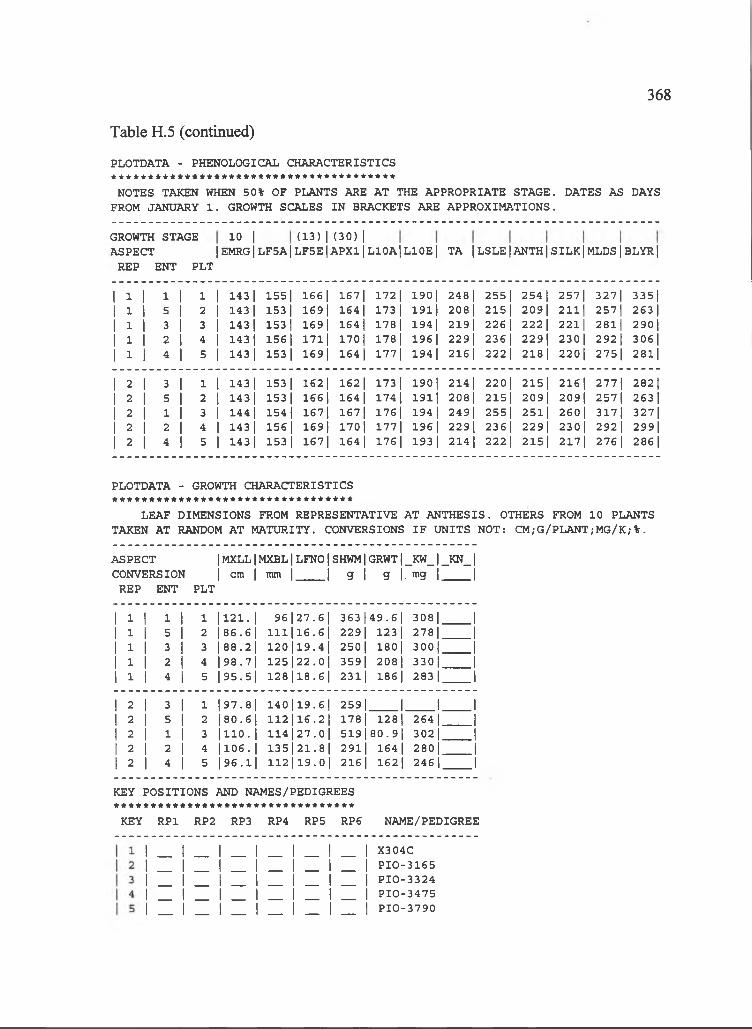
368
Table H.5 (continued)
PLOTDATA - PHENOLOGICAL CHARACTERISTICS ***************************************
NOTES TAKEN WHEN 50% OF PLANTS ARE AT THE APPROPRIATE STAGE. DATES AS DAYS FROM JANUARY 1 . GROWTH SCALES IN BRACKETS ARE APPROXIMATIONS.
GROWTH STAGE 10 I (13) I (30 ) IASPECT !1EMRG1LF5A|LF5E|APXl|LlOA]LIOE| TA 1LSLE1ANTH1SILK 1MLDS1BLYRl
REP ENT PLT
1 1 1 1 1 1 1 143 1 1551 166 1 1671 172 1 190 1 248 1 2551 254 1 2571 3271 33511 1 1 5 1 2 1 143 1 153 1 169| 164 I 173 1 19l| 208 I 215 1 209| 2111 2571 263 11 1 1 3 I 3 1 143 1 153 1 169 1 164 I 1781 194 I 219| 226 1 222 1 2211 2 8 l l 290 11 1 1 2 I 4 1 143 1 1561 1711 170 1 178 1 196 1 2291 236 I 2291 2301 292 1 306|1 1 1 4 1 5 1 143 1 153 1 1691 164 1 1771 194 1 216 1 222 1 218 1 220| 2751 28l|
1 2 1 3 1 1 1 143 1 153 1 162 1 162 1 173 1 1901 214 1 2201 2151 2161 2771 28211 2 1 5 1 2 1 143 1 153 1 166 1 164 I 174 1 1 9 l j 208| 215 1 2091 209| 2571 263 I1 3 1 1 1 3 1 144 1 154 1 1671 167 I 176 I 194 I 249| 255 1 2511 260| 3171 32711 2 1 2 I 4 1 143 1 156 1 169 1 170 1 1771 196 1 229 1 2361 2291 2301 2921 29911 2 1 4 I 5 1 143 1 153 1 167 I 164 1 176 I 193 I 214 I 2221 215| 217| 276 1 286|
PLOTDATA - GROWTH CHARACTERISTICS *********************************
LEAF DIMENSIONS FROM REPRESENTATIVE AT ANTHESIS. OTHERS FROM 10 PLANTS TAKEN AT RANDOM AT MATURITY. CONVERSIONS IF UNITS NOT: CM;G/PLANT;MG/K;%.
ASPECT IMXLL|MXBL|LFNO|SHWM|GRWT|_KW_|_KN_|CONVERSION I cm I mm j | g j g |. mg j j
REP ENT PLT
1 1 1 1 1 1 |121.| 96127.61 363 149 .61 3081 11 1 1 5 1 2 186.61 l l l j 1 6 . 6 | 2291 123 1 278 1 11 1 1 3 I 3 |88.2| 120|1 9 .4 1 250 I 180 1 3001 11 1 1 2 1 4 | 98 .7 l 1 2 5 1 2 2 .o j 359| 208 1 3301 11 1 1 4 1 5 | 95 .5 l 128 118 .6 I 2311 186 1 283 1 1
1 2 1 3 1 1 197.81 1 4 0 1 1 9 .6l 2591 1 1 11 2 1 5 I 2 180.61 I I 2 I I 6 . 2 I 178 I 1281 264 1 11 2 1 1 I 3 | 1 1 0 .1 114|27.0| 5191 80.91 3021 11 2 I 3 1 4 1106.1 135|21.8| 291| 164 I 2801 11 2 1 4 1 5 1 9 6 .1| 1 1 2 | l9 .0 l 216 I 162 I 2461 1
KEY POSITIONS AND NAMES/PEDIGREES * * * * * * * * * * * * * * * * * * * * * * * * * * * * * * * * *
KEY RPl RP2 RP3 RP4 RP5 RP6 NAME/PEDIGREE
X304CPIO -3165PIO -3324PIO -3475PIO -3790

369
IBSNAT REDUCED DATA SET FOR MODELLING CROP GROWTH AND DEVELOPMENT PLOTDATA REQUIRED FOR FIELD EXPERIMENTS
Table H.6 Maize data from Kuiaha Experiment Site, control photoperiod treatment.
GENERAL
PERSONNELRESEARCHER: INSTITUTION:
R ich a rd O gosh i IBSNAT
EXPERIMENT TITLE: ID :
IBSNAT DAYLENGTH;SUMMER;MAIZE 1990 IDSM90K0
TREATMENTSGENOTYPES: 5MANAGEMENT: 0
LOCATIONNAME: K uiaha E xp er im en ta l S i t e
PLOTS*****
PLANTING DATE
PLANT DENSITY (PLANTS/M2)
May 1 7 , 1990
6 .6 7
ORGANISATIONNO.OF ROWS ( # ) :ROW LENGTH (M ):ROW SPACING (CM): ORIENTATION OF ROWS: ALONG OR ACROSS DRAINS: SPACE BETWEEN PLOTS (CM) GROSS AREA ( M 2 ) :
HARVESTNO.OF ROWS:ROW LENGTH (M ):AREA ( M 2 ) :METHOD:
2375E-Wn .a .04 .5
121 .5hand
RANDOMIZATION/REPLICATIONDESIGN: RCBNO.OF REPS.-SOWN: 2
-HARVESTED: 2
PROBLEMS********

370
Table H.6 (continued)
PLOTDATA - PHENOLOGICAL CHARACTERISTICS * * * * * * * * * * * * * * * * * * * * * * * * * * * * * * * * * * * * * * *
NOTES TAKEN WHEN 50% OF PLANTS ARE AT THE APPROPRIATE STAGE. DATES AS DAYS FROM JANUARY 1 . GROWTH SCALES IN BRACKETS ARE APPROXIMATIONS.
GROWTH STAGE 1I 10 1 1 (13) 1 (30 ) 1 1 1 1 11 1 1 1 1ASPECT 1EMRG1LF5A|LF5E1APXl|L10A|LlOE| TA 1LSLEjlANTHl-SILKl MLDSl BLYRl
REP ENT PLT
1 1 1 5 1 1 11 142 1 150 1 1651 160 1 170 1 1851 1901 199|1 193 1 194 1 243 1 25111 1 1 4 1 3 1 142 1 153 1 164 I 164 I 174 1 188 I 206| 223 11 2081 208| 263 1 273 11 1 1 3 1 3 1I 142 1 152 1 162 1 162 1 170 I 184 I 193 1 200|1 196 1 197| 250 I 254]1 1 1 1 I 4 11 142 1 152 1 1611 163 I 173 1 184 I 205| 214 1 2081 207| 267| 274 I1 1 1 3 1 5 11 142 1 150 1 159| 1571 168 1 181'j 197 1 204 1 198 1 197| 2551 263 I
1 3 1 3 1 1 1i 1421 153 1 163 1 164 1 173 1 1871 205 1 223 11 2071 2071 263 1 27111 3 1 5 I 3 11 142 1 150 1 1621 159 I 170 1 184 I 190 I 199 1 192 1 193 I 243 1 25111 3 1 3 I 3 11 142 1 151| 164 1 164 I 169| 188| 202 I 207 1 304 1 205| 2551 263 11 3 1 4 1 4 11 1421 153 1 162 I 160 I 173 1 184 1 194 I 200 1 197 1 197| 2471 25111 3 1 1 j 5 11 142 1 150 I 159 1 163 1 1701 184 1 204 1 214 1 3051 207| 256 I 263 1
PLOTDATA - GROWTH CHARACTERISTICS
LEAF DIMENSIONS FROM REPRESENTATIVE AT ANTHESIS. OTHERS FROM 10 PLANTS TAKEN AT RANDOM AT MATURITY. CONVERSIONS IF UNITS NOT: CM;G/PLANT;MG/K;%.
ASPECT IMXLL|MXBL|LFNO|SHWM|GRWT|_KW_|_KN_|CONVERSION I cm I mm j j g j g | mg j j
REP ENT PLT
1 1 1 5 1 1 170.71 92 1|14.21 1611 114 1 2951 11 1 1 4 1 2 |88.6| 107 |18.61 243 I 1811 3431 11 1 1 3 1 3 | 74 .6 l 113 1115.21 190 1 145 I 3131, 11 1 1 1 1 4 | 93 .8 l 100 1|19.81 262| 155 1 3071 11 1 1 3 1 5 | 83 .5 l 124 |18.21 2521 186 1 343 1 1
1 3 1 3 1 1 187.51 1211|18.81 2591 193 1 3151 11 3 1 5 I 2 | 75 .3 l 111!|14.01 159| 130 1 3141 11 3 1 3 1 3 | 74 .7 l 110||17.21 2111 163 1 353 1 11 3 1 4 1 4 174.61 106 |15.41 1791 133 1 3881 11 3 1 1 1 5 1102.1 106 | 20.0 l 336| 1711 2921 1
KEY POSITIONS AND NAMES/PEDIGREES *********************************
KEY RPl RP2 RP3 RP4 RP5 RP6 NAME/PEDIGREE
X304CP IO -3165PIO -3324P IO -3475PIO -3790

371
IBSNAT REDUCED DATA SET FOR MODELLING CROP GROWTH AND DEVELOPMENT PLOTDATA REQUIRED FOR FIELD EXPERIMENTS
Table H.7 Maize data from Kuiaha Experiment Site, natural photoperiod treatment.
GENERAL
PERSONNELRESEARCHER:INSTITUTION:
R ich a rd O gosh i IBSNAT
EXPERIMENT TITLE: ID:
IBSNAT DAYLENGTH/SUMMER;MAIZE 1990 IDSM90K1
TREATMENTSGENOTYPES: 5MANAGEMENT: 0
LOCATIONNAME: K uiaha E xp er im en ta l S i t e
PLOTS* * * * *
PLANTING DATE
PLANT DENSITY (PLANTS/M2)
May 17 , 1990
6 .6 7
ORGANISATIONNO.OF ROWS ( # ) : 2ROW LENGTH (M ): 3ROW SPACING (CM ): 75ORIENTATION OF ROWS: E-WALONG OR ACROSS DRAINS: n .a .SPACE BETWEEN PLOTS (CM ): 0GROSS AREA ( M 2 ) : 4 .5
HARVESTNO.OF ROWS: ROW LENGTH (M) AREA (M 2 ) : METHOD:
121 .5hand
RANDOMIZATION/REPLICATIONDESIGN: RCBNO.OF REPS.-SOWN: 2
-HARVESTED: 2
PROBLEMS********
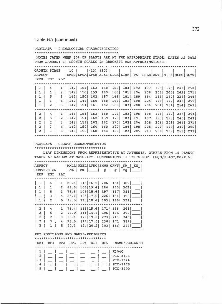
372
PLOTDATA - PHENOLOGICAL CHARACTERISTICS
Table H.7 (continued)
NOTES TAKEN WHEN 50% OF PLANTS ARE AT THE APPROPRIATE STAGE. DATES AS DAYS FROM JANUARY 1 . GROWTH SCALES IN BRACKETS ARE APPROXIMATIONS.
GROWTH STAGE | 10 | | ( 1 3 ) | ( 3 0 ) | I I I I I I | |ASPECT |E M R G |L F 5A |L F 5E |A P X 1|L 10A |L 10E | TA jL SL E|A N TH jSIL K [MLDS|BLYRj
REP ENT PLT
1 1 4 1 1 1 142 1 1511 162 1 160 1 169| 183 1 192 1 197 1 195 1 195 1 240| 250 11 1 1 1 2 1 142 1 150 1 159 1 160| 166| 18l| 204 1 208| 206 1 205| 262 1 271|1 1 5 I 3 1 142 1 150 I 162 I 157 1 166| 181| 189( 194 I 191| 190 1 239| 244 11 1 3 1 4 1I 142 1 149| 160 I 160| 169| 182| 198 1 204 1 199| 199| 248 1 255|1 1 2 1 5 11 1421 151| 1 6 1 1 162 1 169| 183 1 200 I 206 1 204 I 204 I 254 I 263 1
2 1 4 1 1 11 143 1 1511 163 1 160| 174 1 183 1 196 1 198 1 198 1 197 1 248| 254 12 1 5 1 2 11 142| 151| 162 1 159 1 170 1 183 1 1911 197 I 193 1 193 1 240| 243 12 1 2 1 3 11 1421 153 1 162 1 162 1 170| 183 I 204 1 208 I 206| 205| 261| 271|2 1 3 I 4 11 1421 150 1 160 1 160 I 170 I 184 I 198 I 205| 200| 199| 247| 250 12 1 1 I 5 11 143 1 150 1 160 I 164 I 169| 183 I 205| 213 1 208| 209| 263 I 272 1
PLOTDATA - GROWTH CHARACTERISTICS
LEAF DIMENSIONS FROM REPRESENTATIVE AT ANTHESIS. OTHERS FROM 10 PLANTS TAKEN AT RANDOM AT MATURITY. CONVERSIONS IF UNITS NOT: CM;G/PLANT;MG/K;%.
ASPECT IMXLL|MXBL|LFNO|SHWM|GRWT|_KW_|_KN_|CONVERSION I cm I mm j | g j g | mg j j
REP ENT PLT
1 1 1 4 1 1 |80.6| 1 1 8 1 1 6 .2l 206 1 1611 3021 11 1 1 1 1 2 |89.5| 106|19.4| 266 I 170 I 3031 11 1 1 5 1 3 |78.8| 101|15.6| 197 I 1171 311| 11 1 1 3 1 4 |85.0| 125|17.6| 226 1 1861 3501 J1 1 1 2 1 5 |98.5| 130|18.6| 303| 195 1 3511 1
1 3 1 4 1 1 1 7 8 .4| 111115.61 1711 138 1 2651 J1 2 1 5 1 2 | 76 .0 l 111|14.8| 196 1 1351 3021 11 2 1 2 1 3 | 85 .6 l 127|19.6| 273 1 213 1 343 1 11 2 1 3 1 4 |78.5| 1 1 6 1 1 7 .Ol 2381 1711 3291 1I 2 1 1 I 5 |90.3| 124|20.2| 303| 1861 2991 1
KEY POSITIONS AND NAMES/PEDIGREES * * * * * * * * * * * * * * * * * * * * * * * * * * * * * * * * *
KEY RPl RP2 RP3 RP4 RP5 RP6 NAME/PEDIGREE
X304CP IO -3165PIO -3324PIO -3475PIO -3790

373
IBSNAT REDUCED DATA SET FOR MODELLING CROP GROWTH AND DEVELOPMENT PLOTDATA REQUIRED FOR FIELD EXPERIMENTS
Table H.8 Maize data from Kuiaha Experiment Site, 14 h photoperiod treatment.
GENERAL
PERSONNELRESEARCHER:INSTITUTION:
R ich a rd O gosh i IBSNAT
EXPERIMENT TITLE: ID :
IBSNAT DAYLENGTH/SUMMER;MAIZE 1990 IDSM90K2
TREATMENTSGENOTYPES: 5MANAGEMENT: 0
LOCATIONNAME: K uiaha E xp er im en ta l S i t e
PLOTS* * * * *
PLANTING DATE
PLANT DENSITY (PLANTS/M2)
May 17 , 1990
6 .6 7
ORGANISATIONNO.OF ROWS ( # ) : 2ROW LENGTH (M ): 3ROW SPACING (CM ): 75ORIENTATION OF ROWS: E-WALONG OR ACROSS DRAINS: n .a .SPACE BETWEEN PLOTS (CM ): 0GROSS AREA ( M 2 ) : 4 .5
HARVESTNO.OF ROWS: ROW LENGTH (M) AREA ( M 2 ) : METHOD:
121 .5hand
RANDOMIZATION/REPLICATIONDESIGN: RCBNO.OF REPS.-SOWN: 2
-HARVESTED: 2
PROBLEMS********
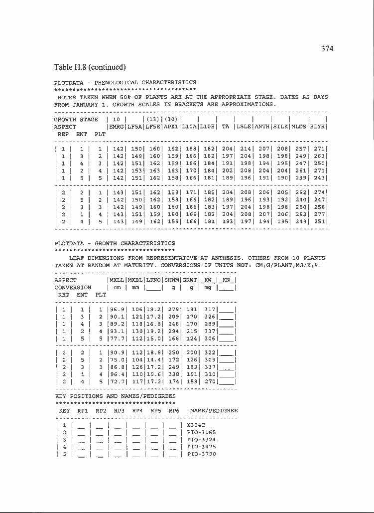
374
Table H,8 (continued)
PLOTDATA - PHENOLOGICAL CHARACTERISTICS ***************************************
NOTES TAKEN WHEN 50% OF PLANTS ARE AT THE APPROPRIATE STAGE. DATES AS DAYS FROM JANUARY 1 . GROWTH SCALES IN BRACKETS ARE APPROXIMATIONS.
GROWTH STAGE | 10 | | (1 3 )| (3 0 )| I I I I I I I IASPECT |EMRGtLF5AlLF5E|APXl|L10A|L10E| TA |LSLEjANTH|SILKjMLDSjBLYRj
REP ENT PLT
1 1 1 1 1 1 142 1 150 1 160 1 1621 168 1 182 1 204 1 214 1 2071 2081 2571 27111 1 3 1 2 1 142 1 149| 160 I 159 1 166 I 182 I 197| 204 I 198 I 198 I 249| 263 11 1 4 1 3 11 142 1 151| 162 I 159 I 166 1 184 I 1 9 l j 198 I 194 I 195 I 247| 250|1 1 2 1 4 11 142] 153 1 163 1 163 1 170 I 184 1 202 I 208| 204 1 204 1 261| 27111 1 5 1 5 11 142 1 1511 162 I 158 1 166 1 181| 189| 196 1 1 9 1 1 190| 2391 243 1
2 1 2 1 1 !1 143 1 1511 162 1 1591 1711 185 1 204 1 208 1 206 1 2051 262 1 274 12 1 5 1 2 11 1421 150 1 162 1 158 1 166 1 182 1 189| 196 I 193 1 192 I 240 I 24712 1 3 1 3 1 142 1 149| 160 I 160 I 166 I 183 1 197| 204 I 198 I 198 1 250 I 256 12 1 1 I 4 1 143 1 151| 1591 160 I 1661 182| 204 1 2081 207| 206| 263 1 27712 1 4 1 5 1 143 1 1491 162 I 159 I 166 I 1811 193 1 1971 194 I 195| 243 1 2511
PLOTDATA - GROWTH CHARACTERISTICS *********************************
LEAF DIMENSIONS FROM REPRESENTATIVE AT ANTHESIS. OTHERS FROM 10 PLANTS TAKEN AT RANDOM AT MATURITY. CONVERSIONS IF UNITS NOT: CM;G/PLANT;MG/K;%.
ASPECT IMXLL|MXBL|LFNO|SHWM|GRWT|_KW_|_KN_|CONVERSION 1 cm I mm j | g j g j mg j j
REP ENT PLT
1 1 1 1 1 1 | 96 .9 l 1 0 6 1 1 9 .2l 2791 1811 3171 11 1 1 3 1 2 | 9 0 .l l 121|17.2| 2091 170 I 3261 11 1 1 4 1 3 189.21 118|16.8| 248 1 170 I 2891 11 1 1 2 1 4 | 9 3 .l l 1 3 0 1 1 9 .2| 294 I 2151 3371 11 1 1 5 1 5 177.71 112|15.0| 168 1 124 1 3061 1
1 2 1 2 1 1 190.91 112118.81 250 1 200 1 3221 11 2 1 5 I 2 | 75 .0 l 104|14.4| 172 1 126 1 3091 1I 2 1 3 1 3 l8 6 .8 l 1 2 6 1 1 7 .2| 2491 1891 3371 11 3 1 1 1 4 | 96 .4 l 110|19.6| 3381 1911 3101 11 2 1 4 1 5 172.71 117|17.2| 174 I 153 1 2701 1
KEY POSITIONS AND NAMES/PEDIGREES * * * * * * * * * * * * * * * * * * * * * * * * * * * * * * * * *
KEY RPl RP2 RP3 RP4 RP5 RP6 NAME/PEDIGREE
I 1 I 21 3I 4I 5
I X304C I P IO -3165 I PIO -3324 1 P IO -3475 I P IO -3790

375
IBSNAT REDUCED DATA SET FOR MODELLING CROP GROWTH AND DEVELOPMENT PLOTDATA REQUIRED FOR FIELD EXPERIMENTS
Table H.9 Maize data from Kuiaha Experiment Site, 17 h photoperiod treatment.
GENERAL
PERSONNELRESEARCHER:INSTITUTION:
R ich a rd O gosh i IBSNAT
EXPERIMENT TITLE: ID :
IBSNAT DAYLENGTH;SUMMER;MAIZE 1990 IDSM90K3
TREATMENTSGENOTYPES: 5MANAGEMENT: 0
LOCATIONNAME: K uiaha E xp er im en ta l S i t e
PLOTS* * * * *
PLANTING DATE
PLANT DENSITY (PLANTS/M2)
May 17 , 1990
6 .6 7
ORGANISATIONNO.OF ROWS ( # ) :ROW LENGTH (M ):ROW SPACING (CM ): ORIENTATION OF ROWS: ALONG OR ACROSS DRAINS: SPACE BETWEEN PLOTS (CM) GROSS AREA ( M 2 ) :
HARVESTNO.OF ROWS:ROW LENGTH (M ):AREA ( M 2 ) :METHOD:
2375E-Wn .a .04 .5
121 .5hand
RANDOMIZATION/REPLICATIONDESIGN: RCBNO.OF REPS.-SOWN: 2
-HARVESTED: 2
PROBLEMS********
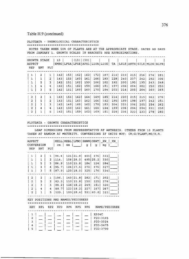
376
PLOTDATA - PHENOLOGICAL CHARACTERISTICS
Table H.9 (continued)
NOTES TAKEN WHEN 50% OF PLANTS ARE AT THE APPROPRIATE STAGE. DATES AS DAYS FROM JANUARY 1 . GROWTH SCALES IN BRACKETS ARE APPROXIMATIONS.
GROWTH STAGE | 10 | | (13) | (30 ) | | | | { | | | |ASPECT |EMRG|LF5AlLF5E|APXl|L10AiL10El TA jLSLE|ANTH|SILKjMLDS|BLYR|
REP ENT PLT
1 1 2 1 1 !1 142 1 153 1 162 1 162 1 172 1 187| 214 1 219| 215| 216 1 274 1 281|1 1 1 1 2 11 143 1 153 1 160 1 1611 166 1 183 1 228| 240 1 237| 242 1 292| 306 I1 1 5 1 3 1 1421 1511 162 1 159 1 166 1 182 I 192 1 200| 195 1 195| 243 i 248|1 1 4 1 4 1 1421 151| 162 1 159 1 166 1 18l| 197| 206 I 204 1 202 1 250 1 255|1 1 3 1 5 1 1421 1511 160 I 160 I 170 I 184 1 203 1 214 1 205| 204 1 260| 265|
2 1 2 1 1 1 143 1 153 1 162 1 164 1 169| 185| 214 1 220| 215| 215| 263 1 276 12 1 5 I 2 1 143 1 1511 162 I 162 1 166 1 182| 195 I 199| 198 1 197 I 242 I 251|2 1 3 I 3 1 142 1 149| 160| 162 1 170 I 183 I 204 1 223 1 206| 205 I 254 I 262 12 1 4 1 4 1 143 1 150 1 162 1 161| 168 1 184 1 199| 206 1 204 I 204 1 251| 256 I2 1 1 I 5 1 142 1 1511 159 1 162 I 169 1 181| 228 I 236 I 233 1 233 1 278| 283 1
PLOTDATA - GROWTH CHARACTERISTICS *********************************
LEAF DIMENSIONS FROM REPRESENTATIVE AT ANTHESIS. OTHERS FROM 10 PLANTS TAKEN AT RANDOM AT MATURITY. CONVERSIONS IF UNITS NOT: CM;G/PLANT;MG/K;%.
ASPECT CONVERSION
REP ENT
IMXLLIMXBL|LFNO|SHWM|GRWT|_KW_|_KN_| I cm I mm j | g j g | mg j j
PLT
1 1 1 2 1 1 |94.4| 121|21.8| 4011 1761 3331 11 1 1 1 1 2 |114.| 108|28.0| 495125 .21 3301 11 1 1 5 1 3 |86.9| 1 1 0 | l5 .8 i 184 1 124 1 2841 11 1 1 4 1 4 |95.7| 1 2 4 1 1 7 .6| 272 1 176 I 3271 11 1 1 3 I 5 |87.9| 120|18.0| 3251 176 1 3341 1
1 2 1 2 1 1 1106.1 1 4 0 1 2 1 .8l 2821 1711 2921 11 2 1 5 1 2 | 8 3 .3 l 110|15.8| 150 1 1251 2781 11 2 1 3 1 3 |88.2| 126|18.2| 249 I 1511 3201 11 2 j 4 1 4 |88.7| 1 2 3 1 1 8 .2l 2271 1671 2671 11 2 I 1 I 5 1 1 2 9 .1 10 9 | 28 .4 I 5511 6 0 .8| 3151 1
KEY POSITIONS AND NAMES/PEDIGREES * * * * * * * * * * * * * * * * * * * * * * * * * * * * * * * * *
KEY RPl RP2 RP3 RP4 RP5 RP6 NAME/PEDIGREE
X304CPIO-31G5PIO -3324PIO -3475PIO -3790

377
IBSNAT REDUCED DATA SET FOR MODELLING CROP GROWTH AND DEVELOPMENT PLOTDATA REQUIRED FOR FIELD EXPERIMENTS
Table H.IO Maize data from Kuiaha Experiment Site, 20 h photoperiod treatment.
GENERAL* * * * * * *
PERSONNELRESEARCHER:INSTITUTION:
R ich a rd O gosh i IBSNAT
EXPERIMENTTITLE:ID :
IBSNAT DAYLENGTH/SUMMER;MAIZE 1990 IDSM90K4
TREATMENTSGENOTYPES: 5MANAGEMENT: 0
LOCATIONNAME: K uiaha E xp er im en ta l S i t e
PLOTS
ORGANISATIONNO.OF ROWS ( # ) : 2ROW LENGTH (M ): 3ROW SPACING (CM ): 75ORIENTATION OF ROWS: E-WALONG OR ACROSS DRAINS: n .a .SPACE BETWEEN PLOTS (CM): 0GROSS AREA ( M 2 ) : 4 .5
HARVESTNO.OF ROWS: ROW LENGTH (M) AREA (M 2 ) : METHOD:
124 .5hand
RANDOMIZATION/REPLICATIONDESIGN: RCBNO.OF REPS.-SOWN: 2
-HARVESTED: 2
PROBLEMS* * * * * * * *
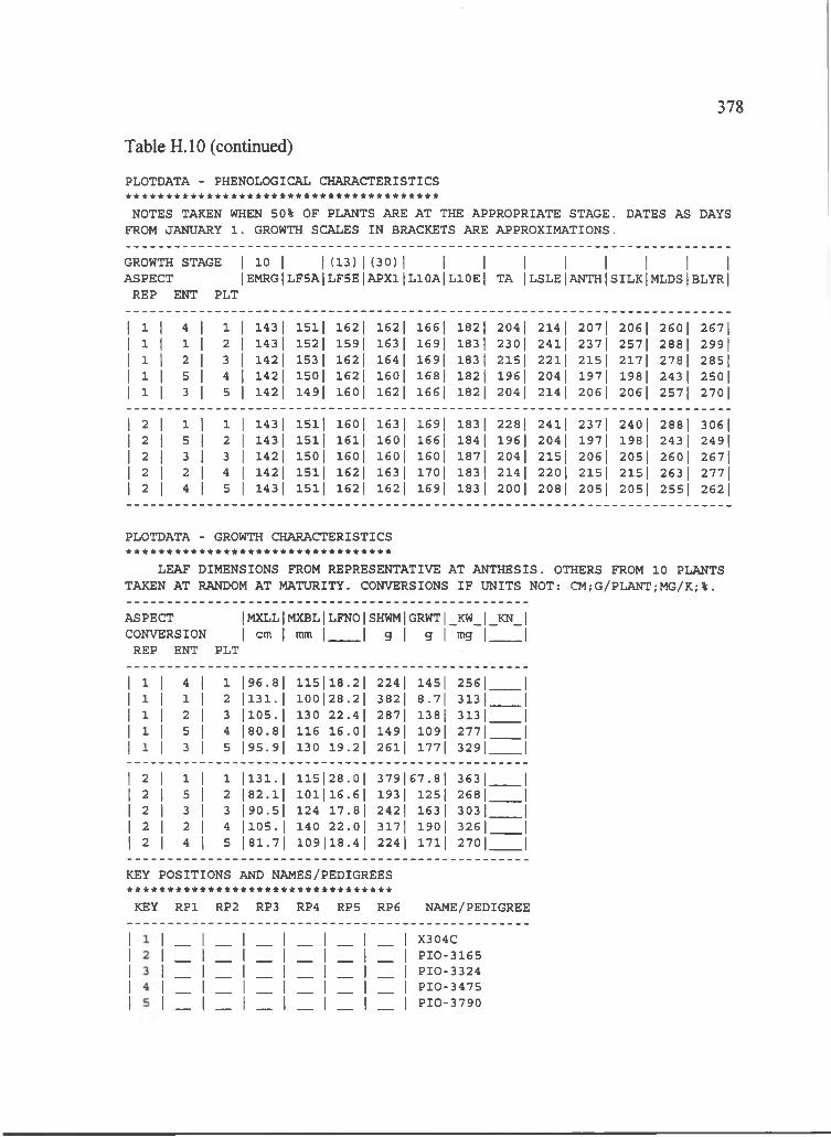
378
PLOTDATA - PHENOLOGICAL CHARACTERISTICS
Table H.IO (continued)
NOTES TAKEN WHEN 50% OF PLANTS ARE AT THE APPROPRIATE STAGE. DATES AS DAYS FROM JANUARY 1 . GROWTH SCALES IN BRACKETS ARE APPROXIMATIONS.
GROWTH STAGE 1 10 | | (1 3 ) | (3 0 ) | I | | | | | | |ASPECT |E M R G |L F 5A |L F 5E |A P X 1|L 10A |L 10E | TA |L S L E 1ANTHjSILK|MLDS|BLYRj
REP ENT PLT
1 1 1 4 1 1 11 143 1 1511 1621 162 1 1661 1821 2 0 4 1 2 1 4 1 2071 2061 2601 26711 1 1 1 I 2 11 143 1 152 1 1 5 9 | 163 I 1 6 9 | 1 8 3 | 2 3 0 | 2 4 1 | 2371 2 5 7 | 2 8 8 | 29911 1 1 2 1 3 11 142 1 153 1 162 I 164 I 1 6 9 | 183 1 2151 2211 2151 2 1 7 | 2 7 8 | 2 8 5 |1 1 1 5 1 4 11 142 1 1501 1621 16 0 I 1 6 8 | 1 8 2 ] 1 9 6 1 2 0 4 1 1971 1 9 8 | 24 3 1 2 5 0 11 1 1 3 j 5 11 1421 1 4 9 | 16 0 I 16 2 I 1 6 6 | 1 8 2 1 2 0 4 I 2 1 4 1 2 0 6 1 2 0 6 | 2571 2 7 0 1
1 2 1 1 1 1 1 143 1 1511 160 1 163 1 1691 183 1 2 2 8 1 2411 2371 2401 2881 3 0 6 11 2 1 5 I 2 1 143 1 1511 1 6 1 1 16 0 I 1 6 6 | 1 8 4 I 1 9 6 1 2 0 4 I 1971 19 8 1 24 3 1 2 4 9 |1 2 I 3 I 3 1 142 1 15 0 1 1 6 0 | 160 I 1 6 0 | 1 8 7 | 2 0 4 I 2151 2 0 6 | 2 0 5 | 2 6 0 I 2 6 7 ]1 2 I 2 1 4 1 142 1 1511 162 I 163 I 17 0 I 1 8 3 | 2 1 4 I 2201 2151 2151 26 3 I 2 7 7 11 2 j 4 j 5 1 143 1 1511 162 I 162 I 1 6 9 | 183 I 2 0 0 | 2 0 8 1 2051 2051 2 5 5 | 2 6 2 1
PLOTDATA - GROWTH CHARACTERISTICS
LEAF DIMENSIONS FROM REPRESENTATIVE AT ANTHESIS. OTHERS FROM 10 PLANTS TAKEN AT RANDOM AT MATURITY. CONVERSIONS IF UNITS NOT: CM;G/PLANT;MG/K;%.
ASPECT IMXLLIMXBLILFNOISHWMIGRWTI_KW_I_KN_ICONVERSION I cm I mm j j g j g | mg j j
REP ENT PLT
1 1 1 4 1 1 196.81 1151|18,.2| 224 1 1451 2561 11 1 1 1 I 2 1131.1 100 1|28,.2| 382| 8.71 3131 11 1 1 2 I 3 | 1 0 5 .1 130 |22,•41 287| 138 1 3131 11 1 1 5 I 4 180.81 116 |16,•o| 149 1 109| 2771 11 1 1 3 1 5 195.91 130 |19,.21 261| 1771 3 2 9 l _ _ l
1 2 1 1 1 1 1131.1 115 1|28,•01 3791 6 7 .8 1 3631 11 2 1 5 I 2 182.11 101||16,.61 193 I 125| 2681 11 2 1 3 1 3 190.51 124 |17,.81 242 I 163 I 3031 11 2 1 2 I 4 | 1 0 5 .1 140 |22,•o| 3171 190 1 326| 1I 2 I 4 1 5 | 81 .7 l 109 |18 •4| 224 1 1711 270 1 1
KEY POSITIONS AND NAMES/PEDIGREES * * * * * * * * * * * * * * * * * * * * * * * * * * * * * * * * *
KEY RPl RP2 RP3 RP4 RP5 RP6 NAME/PEDIGREE
X304CP IO -3165PIO -3324PIO -3475PIO -3790
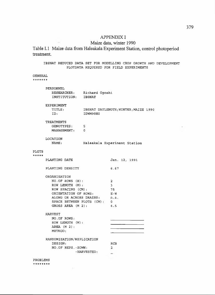
379
APPENDIX I Maize data, winter 1990
Table I.l Maize data from Haleakala Experiment Station, control photoperiod treatment.
IBSNAT REDUCED DATA SET FOR MODELLING CROP GROWTH AND DEVELOPMENT PLOTDATA REQUIRED FOR FIELD EXPERIMENTS
GENERAL
PERSONNELRESEARCHER:INSTITUTION:
R ich a rd O gosh i IBSNAT
EXPERIMENT TITLE: ID :
IBSNAT DAYLENGTH/WINTER;MAIZE 1990 IDWM90H0
TREATMENTSGENOTYPES: 5MANAGEMENT: 0
LOCATIONNAME: H a le a k a la E xperim en t S t a t io n
PLOTS* * * * *
PLANTING DATE
PLANTING DENSITY
Jan . 12 , 1991
6 .6 7
ORGANISATIONNO.OF ROWS ( # ) : 2ROW LENGTH (M ): 3ROW SPACING (CM ): 75ORIENTATION OF ROWS: E-WALONG OR ACROSS DRAINS: n .a .SPACE BETWEEN PLOTS (CM ): 0GROSS AREA ( M 2 ) : 4 .5
HARVESTNO.OF ROWS:ROW LENGTH (M ): AREA ( M 2 ) : METHOD:
RANDOMIZATION/REPLICATIONDESIGN:NO.OF REPS.-SOWN:
-HARVESTED:
RCB2
PROBLEMS********

380
PLOTDATA - PHENOLOGICAL CHARACTERISTICS
Table I.l (continued)
NOTES TAKEN WHEN 50% OF PLANTS ARE AT THE APPROPRIATE STAGE. DATES AS DAYS FROM JANUARY 1 . GROWTH SCALES IN BRACKETS ARE APPROXIMATIONS.
GROWTH STAGE | 10 [ [ (13) | (30) | | | | | | | | |ASPECT |EMRG|LF5A|LF5E|APX1|L10A|L10E| TA |LSLE1ANTHjSILK|MLDS|BLYR|
REP ENT PLT
1 1 3 1 1 1 19 11 32 1 50 1 46 11 1 4 1 2 1 19 11 35 1 50 1 47 11 1 5 1 3 1 19 11 33 1 51 1 49 11 1 2 1 4 1 19 !1 36 1 50 11 50 11 1 1 1 5 1 20 11 36 1 51 11 50 1
2 1 4 1 1 1 19 !1 33 1 50 1 46 12 1 2 I 2 1 19 i1 34 1 51 1t 52 12 1 5 1 3 1 19 11 33 1 52 1 46 12 1 3 I 4 1 19 11 32 1 50 1 48 12 1 1 1 5 1 20 !1 35 1 51 1 50 1
J I.J I
J I
PLOTDATA - GROWTH CHARACTERISTICS * * * * * * * * * * * * * * * * * * * * * * * * * * * * * * * * *
LEAF DIMENSIONS FROM REPRESENTATIVE AT ANTHESIS. OTHERS FROM 10 PLANTS TAKEN AT RANDOM AT MATURITY. CONVERSIONS IF UNITS NOT: CM;G/PLANT;MG/K;%.
ASPECT CONVERSION
REP ENT PLT
IMXLLIMXBL|LFNO|SHWM|GRWT|_KW_|_KN_|
12345
KEY POSITIONS AND NAMES/PEDIGREES * * * * * * * * * * * * * * * * * * * * * * * * * * * * * * * * *
KEY RPl RP2 RP3 RP4 RP5 RP6 NAME/PEDIGREE
X304CP IO -3165PIO -3324P IO -3475P IO -3790
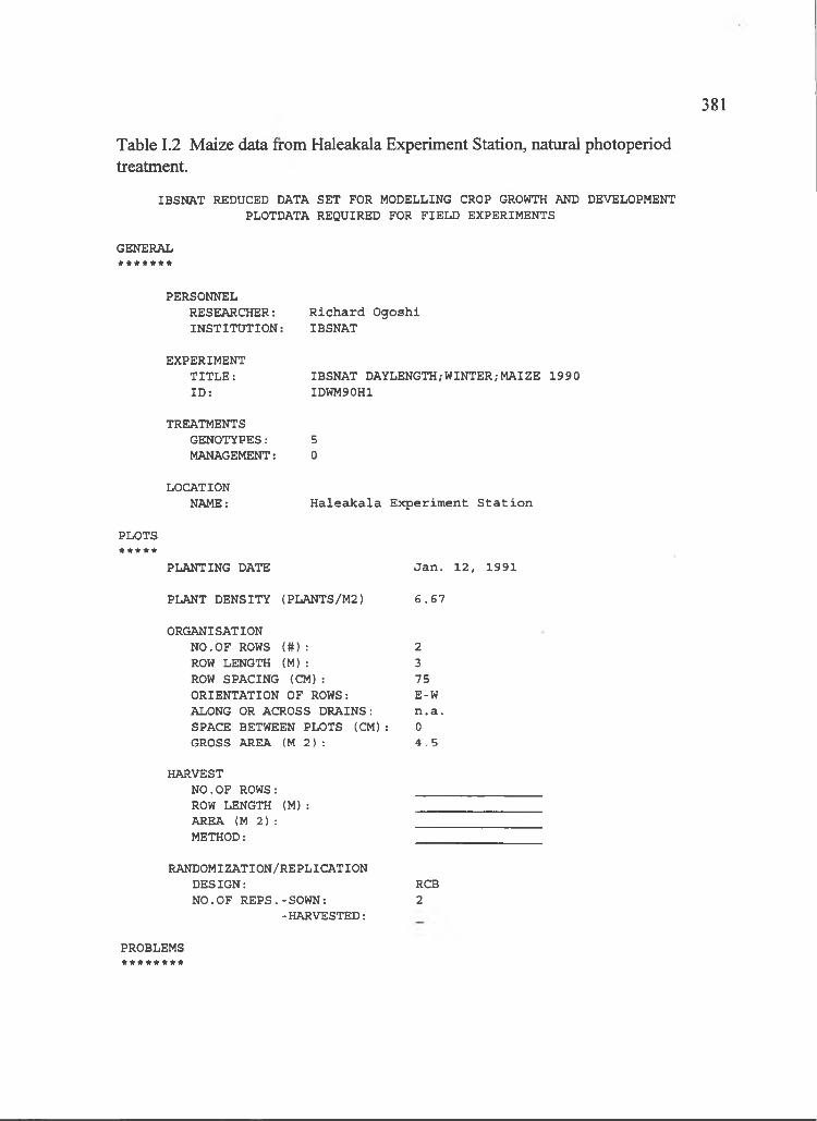
381
IBSNAT REDUCED DATA SET FOR MODELLING CROP GROWTH AND DEVELOPMENT PLOTDATA REQUIRED FOR FIELD EXPERIMENTS
GENERAL
Table 1.2 Maize data from Haleakala Experiment Station, natural photoperiodtreatment.
PERSONNELRESEARCHER:INSTITUTION:
R ich a rd O gosh i IBSNAT
EXPERIMENT TITLE: ID :
IBSNAT DAYLENGTH/WINTER;MAIZE 1990 IDWM90H1
TREATMENTSGENOTYPES: 5MANAGEMENT: 0
LOCATIONNAME: H a lea k a la E xperim ent S t a t io n
PLOTS* * * * *
PLANTING DATE
PLANT DENSITY (PLANTS/M2)
Jan . 12 , 1991
6 .6 7
ORGANISATIONNO.OF ROWS { # ) : 2ROW LENGTH (M ): 3ROW SPACING (CM ): 75ORIENTATION OF ROWS: E-WALONG OR ACROSS DRAINS: n .a .SPACE BETWEEN PLOTS (CM): 0GROSS AREA ( M 2 ) : 4 .5
HARVESTNO.OF ROWS:ROW LENGTH (M) :AREA (M 2) :METHOD:
RANDOMIZATION/REPLICATIONDESIGN:NO.OF REPS.-SOWN:
-HARVESTED:
RCB2
PROBLEMS********

382
Table 1.2 (continued)
PLOTDATA - PHENOLOGICAL CHARACTERISTICS * * * * * * * * * * * * * * * * * * * * * * * * * * * * * * * * * * * * * * *
NOTES TAKEN WHEN 50% OF PLANTS ARE AT THE APPROPRIATE STAGE. DATES AS DAYS FROM JANUARY 1 . GROWTH SCALES IN BRACKETS ARE APPROXIMATIONS.
GROWTH STAGE ASPECT
I 10 I I (13) I (30) I I I I I I I I I|EMRG|LF5A|LF5E|APX1|L10A|L10E| TA 1LSLE[ANTHIsILKIMLDSIBLYRl
REP ENT PLT
1 1 3 1 1 1 19 i1 35 1 51 1 50 11 1 4 1 3 1 19 11 34 1 50 1 45 11 1 1 1 3 1 19 !1 35 1 50 1 50 11 1 3 1 4 1 19 i1 33 1 50 1 46 11 1 5 1 5 1 19 j1 33 1 51 1 44 1
2 1 4 1 1 1 19 1 33 1 50 1 46 12 I 2 1 2 1 19 11 35 1 50 11 51 12 1 3 1 3 1 19 1 32 1 50 11 45 12 1 1 I 4 1 19 11 36 1 50 11 50 12 1 5 1 5 1 19 i1 33 1 52 11 46 1
J I.
J I.
J I.
J I.
PLOTDATA - GROWTH CHARACTERISTICS
LEAF DIMENSIONS FROM REPRESENTATIVE AT ANTHESIS. OTHERS FROM 10 PLANTS TAKEN AT RANDOM AT MATURITY. CONVERSIONS IF UNITS NOT: CM; G/PLANT;M G/K;%.
ASPECT CONVERSION
REP ENT
1MXLL1MXBL1LFNO1SHWM1GRWT1_KW_1_KN _1
PLT
4 2 3 15
12345
J I.
KEY POSITIONS AND NAMES/PEDIGREES * * * * * * * * * * * * * * * * * * * * * * * * * * * * * * * * *
KEY RPl RP2 RP3 RP4 RP5 RP6 NAME/PEDIGREE
X304CPIO -3165PIO -3324PIO -3475PIO -3790

383
IBSNAT REDUCED DATA SET FOR MODELLING CROP GROWTH AND DEVELOPMENT PLOTDATA REQUIRED FOR FIELD EXPERIMENTS
Table 1.3 Maize data from Kuiaha Experiment Site, control photoperiod treatment.
GENERAL
PERSONNELRESEARCHER:INSTITUTION:
R ich a rd O gosh i IBSNAT
EXPERIMENT TITLE: ID :
IBSNAT DAYLENGTH/WINTER;MAIZE 1990 IDWM90K0
TREATMENTSGENOTYPES: 5MANAGEMENT: 0
LOCATIONNAME: Kuiaha E xp er im en ta l S i t e
PLOTS* * * * *
PLANTING DATE
PLANT DENSITY (PLANTS/M2)
Jan . 1 2 , 1991
6 .6 7
ORGANISATIONNO.OF ROWS ( # ) : 2ROW LENGTH (M ): 3ROW SPACING (CM ): 75ORIENTATION OF ROWS: E-WALONG OR ACROSS DRAINS: n .a .SPACE BETWEEN PLOTS (CM ): 0GROSS AREA ( M 2 ) : 4 .5
HARVESTNO.OF ROWS:ROW LENGTH (M ):AREA (M 2 ) :METHOD:
RANDOMIZATION/REPLICATIONDESIGN:NO.OF REPS.-SOWN:
-HARVESTED:
RCB2
PROBLEMS* * * * * * * *
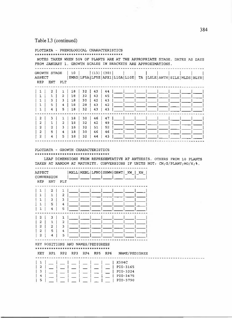
384
PLOTDATA - PHENOLOGICAL CHARACTERISTICS
NOTES TAKEN WHEN 50% OF PLANTS ARE AT THE APPROPRIATE STAGE. DATES AS DAYS FROM JANUARY 1 . GROWTH SCALES IN BRACKETS ARE APPROXIMATIONS.
Table 1.3 (continued)
GROWTH STAGE | 10 | | (1 3 )| (3 0 )| I I I I I I | |ASPECT |EMRG|LF5A|LF5E|APXl|L10A|L10Ei TA jLSLEjANTH|SILK1MLDS|BLYRj
REP ENT PLT
1 1 2 1 1 11 18 1 32 11 43 i1 44 11 1 1 I 2 11 18 1 32 11 43 i1 45 11 1 3 1 3 11 18 I 30 11 42 !1 43 11 1 5 1 4 11 18 1 1 28 j 1 43 i 1 42 11 1 4 1 5 1 18 1i 32 11 43 11 43 1
2 1 3 1 1 1 18 11 30 1 46 1 47 12 I 1 1 2 1 18 11 32 1 42 1 49 12 1 2 I 3 1 18 11 32 1 51 1 52 12 I 5 1 4 1 18 11 30 1 46 1 46 1,2 1 4 1 5 1 18 11 32 1 44 1 43 1
J I.
J ____ I.J ____ I.J ____ I.J ____ I.J ____ I.
PLOTDATA - GROWTH CHARACTERISTICS *********************************LEAF DIMENSIONS FROM REPRESENTATIVE AT ANTHESIS. OTHERS FROM 10 PLANTS
TAKEN AT RANDOM AT MATURITY. CONVERSIONS IF UNITS NOT; CM;G/PLANT;MG/K;%.
ASPECT IMXLL|MXBL|LFNO|SHWM|GRWT|_KW_|_KN_|CONVERSION I I I I I I I I
REP ENT PLT
12345
.1 I. J ..1 I.J I.J I..1 I.
3 1 2 54
1 1 .2 I.3 I.4 I.5 I J I.
KEY POSITIONS AND NAMES/PEDIGREES * * * * * * * * * * * * * * * * * * * * * * * * * * * * * * * * *
KEY RPl RP2 RP3 RP4 RP5 RP6 NAME/PEDIGREE
12345
X304CPIO -3165PIO -3324PIO -3475PIO -3790
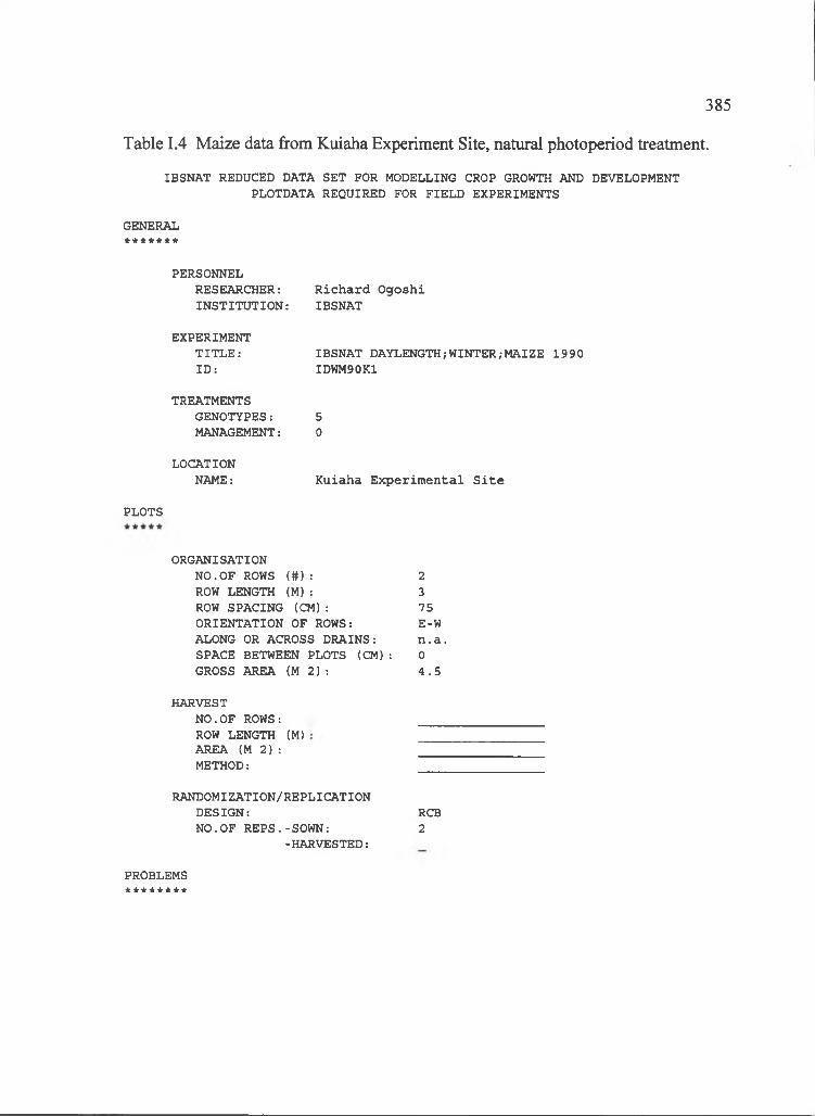
385
IBSNAT REDUCED DATA SET FOR MODELLING CROP GROWTH AND DEVELOPMENT PLOTDATA REQUIRED FOR FIELD EXPERIMENTS
Table 1.4 Maize data from Kuiaha Experiment Site, natural photoperiod treatment.
GENERAL
PERSONNELRESEARCHER: INSTITUTION:
R ich a rd O gosh i IBSNAT
EXPERIMENTTITLE:ID :
IBSNAT DAYLENGTH;WINTER;MAIZE 1990 IDWM90K1
TREATMENTSGENOTYPES: 5MANAGEMENT: 0
LOCATIONNAME: Kuiaha E xp er im en ta l S i t e
PLOTS
ORGANISATIONNO.OF ROWS ( # ) : 2ROW LENGTH (M ): 3ROW SPACING (CM ): 75ORIENTATION OF ROWS: E-WALONG OR ACROSS DRAINS: n .a .SPACE BETWEEN PLOTS (CM): 0GROSS AREA ( M 2 ) : 4 .5
HARVESTNO.OF ROWS: ROW LENGTH (M) AREA (M 2 ) : METHOD:
RANDOMIZATION/REPLICATIONDESIGN:NO.OF REPS.-SOWN:
-HARVESTED:
RCB2
PROBLEMS********

386
Table 1.4 (continued)
PLOTDATA - PHENOLOGICAL CHARACTERISTICS * * * * * * * * * * * * * * * * * * * * * * * * * * * * * * * * * * * * * * *
NOTES TAKEN WHEN 50% OF PLANTS ARE AT THE APPROPRIATE STAGE. DATES AS DAYS FROM JANUARY 1 . GROWTH SCALES IN BRACKETS ARE APPROXIMATIONS.
GROWTH STAGE | 10 | | (1 3 )| (3 0 )| I I I I I I | IASPECT |EMRG|LF5A|LF5E|APXl|L10A|L10E| TA jLSLEjANTH|SILK|MLDSjBLYR|
REP ENT PLT
1 1 3 1 1 11 18 i1 31 11 44 1 42 11 1 2 1 2 11 18 11 32 1 44 1 42 11 1 4 1 3 11 18 11 31 11 43 1 43 11 1 5 1 4 11 18 11 30 1I 44 1 42 t1 1 1 1 5 11 18 1 31 1 43 1 42 1
2 1 2 1 1 11 18 i1 33 11 51 1 52 12 1 3 1 2 11 18 11 30 1t 43 1 42 12 1 1 1 3 11 18 i1 31 11 42 1 43 12 1 5 1 4 11 18 11 30 1! 46 1 43 12 1 4 1 5 11 18 1 32 11 46 1 44 1
J .
PLOTDATA - GROWTH CHARACTERISTICS * * * * * * * * * * * * * * * * * * * * * * * * * * * * * * * * *
LEAF DIMENSIONS FROM REPRESENTATIVE AT ANTHESIS. OTHERS FROM 10 PLANTS TAKEN AT RANDOM AT MATURITY. CONVERSIONS IF UNITS NOT: CM;G/PLANT;MG/K;%.
ASPECT IMXLL|MXBL|LFNO|SHWM|GRWT|_KW_|_KN_|CONVERSION I I I I 1 I I 1
REP ENT PLT
3 245 1
1 I.2 I.3 I.4 I.5 I
J ____ I____ I.J ____ I____ 1.J ____ I____ I.J ____ I____ I.J ____ I____ I.
23 1 54
J I.
KEY POSITIONS AND NAMES/PEDIGREES * * * * * * * * * * * * * * * * * * * * * * * * * * * * * * * * *
KEY RPl RP2 RP3 RP4 RP5 RP6 NAME/PEDIGREE
X304CP IO -3165P IO -3324PIO -3475PIO -3790
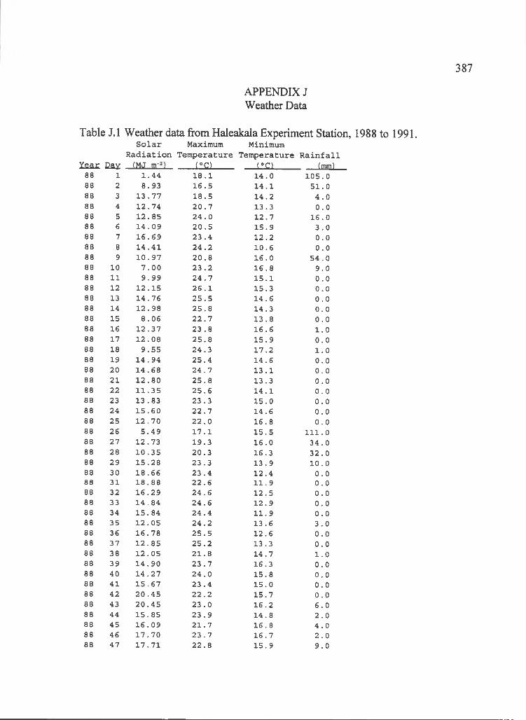
387
a p p e n d ix ; Weather Data
Table J.l Weather data from Haleakala Experiment Station, 1988 to 1991.S o la r Maximum Minimum
R a d ia t io n T em peratu re T em perature R a in f a l l I s a r C a y ( M J _________ ( ° c ) ( ° o ____________(mm)
88 1 1 .4 4 1 8 .1 1 4 .0 1 0 5 .088 2 8 .9 3 1 6 .5 1 4 .1 5 1 .088 3 1 3 .7 7 1 8 .5 1 4 .2 4 .088 4 1 2 .7 4 2 0 .7 1 3 .3 0 .088 5 1 2 .8 5 2 4 .0 1 2 .7 1 6 .088 6 1 4 .0 9 2 0 .5 1 5 .9 3 .088 7 1 6 .6 9 2 3 .4 1 2 .2 0 .088 8 1 4 .4 1 2 4 .2 1 0 .6 0 .088 9 1 0 .9 7 2 0 .8 1 6 .0 5 4 .088 10 7 .0 0 2 3 .2 1 6 .8 9 .088 11 9 .9 9 2 4 .7 1 5 .1 0 .088 12 1 2 .1 5 2 6 .1 1 5 .3 0 .088 13 1 4 .7 6 2 5 .5 1 4 .6 0 .088 14 1 2 .9 8 2 5 .8 1 4 .3 0 .088 15 8 .0 6 2 2 .7 1 3 .8 0 .088 16 1 2 .3 7 2 3 .8 1 6 .6 1 .088 17 1 2 .0 8 2 5 .8 1 5 .9 0 .088 18 9 .5 5 2 4 .3 1 7 .2 1 .088 19 1 4 .9 4 2 5 .4 1 4 .6 0 .088 20 1 4 .6 8 2 4 .7 1 3 .1 0 .088 21 1 2 .8 0 2 5 .8 1 3 .3 0 .088 22 1 1 .3 5 2 5 .6 1 4 .1 0 .088 23 1 3 .8 3 2 3 .3 1 5 .0 0 .088 24 1 5 .6 0 2 2 .7 1 4 .6 0 .088 25 1 2 .7 0 2 2 .0 1 6 .8 0 .088 26 5 .4 9 1 7 .1 1 5 .5 1 1 1 .088 27 1 2 .7 3 1 9 .3 1 6 .0 3 4 .088 28 1 0 .3 5 2 0 .3 1 6 .3 3 2 .088 29 1 5 .2 8 2 3 .3 1 3 .9 1 0 .088 30 1 8 .6 6 2 3 .4 1 2 .4 0 .088 31 1 8 .8 8 2 2 .6 1 1 .9 0 .088 32 1 6 .2 9 2 4 .6 1 2 .5 0 .088 33 1 4 .8 4 2 4 .6 1 2 .9 0 .088 34 1 5 .8 4 2 4 .4 1 1 .9 0 .088 35 1 2 .0 5 2 4 .2 1 3 .6 3 .088 36 1 6 .7 8 2 5 .5 1 2 .6 0 .088 37 1 2 .8 5 2 5 .2 1 3 .3 0 .088 38 1 2 .0 5 2 1 .8 1 4 .7 1 .088 39 1 4 .9 0 2 3 .7 1 6 .3 0 .088 40 1 4 .2 7 2 4 .0 1 5 .8 0 .088 41 1 5 .6 7 2 3 .4 1 5 .0 0 .088 42 2 0 .4 5 2 2 .2 1 5 .7 0 .088 43 2 0 .4 5 2 3 .0 1 6 .2 6 .088 44 1 5 .8 5 2 3 .9 1 4 .8 2 .088 45 1 6 .0 9 2 1 .7 1 6 .8 4 .088 46 1 7 .7 0 2 3 .7 1 6 .7 2 .088 47 1 7 .7 1 2 2 .8 1 5 .9 9 .0
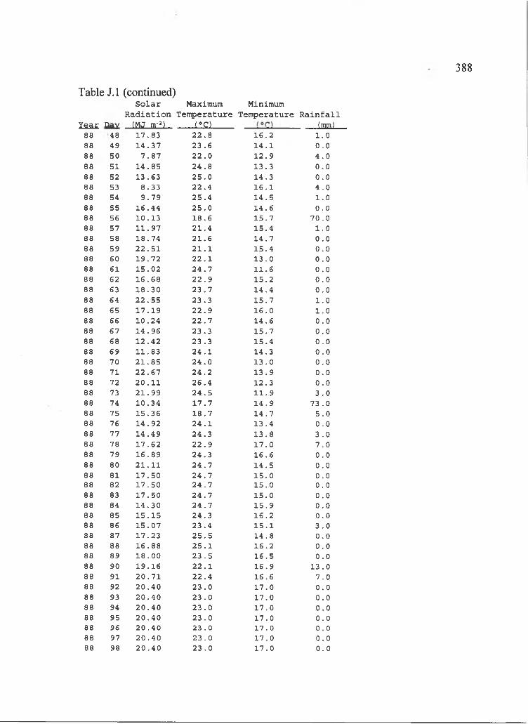
388
Table J. 1 (continued)S o la r Maximum Minimum
R a d ia t io n T em peratu re T em peratu re R a in f a l lY ear Day (MJ m' )________LiiU______ (mm)
88 48 1 7 .8 3 2 2 .8 I S . 2 1 .088 49 1 4 .3 7 2 3 .6 1 4 .1 0 .088 50 7 .8 7 2 2 .0 1 2 .9 4 .088 51 1 4 .8 5 2 4 .8 1 3 .3 0 .088 52 1 3 .6 3 2 5 .0 1 4 .3 0 .088 53 8 .3 3 2 2 .4 1 6 .1 4 .088 54 9 .7 9 2 5 .4 1 4 .5 1 .088 55 1 6 .4 4 2 5 .0 1 4 .6 0 .088 56 1 0 .1 3 1 8 .6 1 5 .7 7 0 .088 57 1 1 .9 7 2 1 .4 1 5 .4 1 .088 58 1 8 .7 4 2 1 .6 1 4 .7 0 .088 59 2 2 .5 1 2 1 .1 1 5 .4 0 .088 60 1 9 .7 2 2 2 .1 1 3 .0 0 .088 61 1 5 .0 2 2 4 .7 1 1 .6 0 .088 62 1 6 .6 8 2 2 .9 1 5 .2 0 .088 63 1 8 .3 0 2 3 .7 1 4 .4 0 .088 64 2 2 .5 5 2 3 .3 1 5 .7 1 .088 65 1 7 .1 9 2 2 .9 1 6 .0 1 .088 66 1 0 .2 4 2 2 .7 1 4 .6 0 .088 67 1 4 .9 6 2 3 .3 1 5 .7 0 .088 68 1 2 .4 2 2 3 .3 1 5 .4 0 .088 69 1 1 .8 3 2 4 .1 1 4 .3 0 .088 70 2 1 .8 5 2 4 .0 1 3 .0 0 .088 71 2 2 .6 7 2 4 .2 1 3 .9 0 .088 72 2 0 .1 1 2 6 .4 1 2 .3 0 .088 73 2 1 .9 9 2 4 .5 1 1 .9 3 .088 74 1 0 .3 4 1 7 .7 1 4 .9 7 3 .088 75 1 5 .3 6 1 8 .7 1 4 .7 5 .088 76 1 4 .9 2 2 4 .1 1 3 .4 0 .088 77 1 4 .4 9 2 4 .3 1 3 .8 3 .088 78 1 7 .6 2 2 2 .9 1 7 .0 7 .088 79 1 6 .8 9 2 4 .3 1 6 .6 0 .088 80 2 1 .1 1 2 4 .7 1 4 .5 0 .088 81 1 7 .5 0 2 4 .7 1 5 .0 0 .088 82 1 7 .5 0 2 4 .7 1 5 .0 0 .088 83 1 7 .5 0 2 4 .7 1 5 .0 0 .088 84 1 4 .3 0 2 4 .7 1 5 .9 0 .088 85 1 5 .1 5 2 4 .3 1 6 .2 0 .088 86 1 5 .0 7 2 3 .4 1 5 .1 3 .088 87 1 7 .2 3 2 5 .5 1 4 .8 0 .088 88 1 6 .8 8 2 5 .1 1 6 .2 0 .088 89 1 8 .0 0 2 3 .5 1 6 .5 0 .088 90 1 9 .1 6 2 2 .1 1 6 .9 1 3 .088 91 2 0 .7 1 2 2 .4 1 6 .6 7 .088 92 2 0 .4 0 2 3 .0 1 7 .0 0 .088 93 2 0 .4 0 2 3 .0 1 7 .0 0 .088 94 2 0 .4 0 2 3 .0 1 7 .0 0 .088 95 2 0 .4 0 2 3 .0 1 7 .0 0 .088 96 2 0 .4 0 2 3 .0 1 7 .0 0 .088 97 2 0 .4 0 2 3 .0 1 7 .0 0 .088 98 2 0 .4 0 2 3 .0 1 7 .0 0 .0
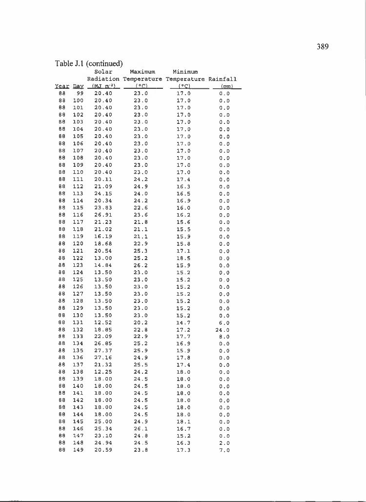
389
Table J.l (continued)S o l a r Maximum Minimum
R a d i a t i o n Temperatur e Temperature R a i n f a l lY ear Dav (MJ m' )__________________ LliHj______(mm)
88 99 2 0 . 4 0 2 3 . 0 1 7 . 0 0 . 088 100 2 0 . 4 0 2 3 . 0 1 7 . 0 0 . 088 101 2 0 . 4 0 2 3 . 0 1 7 . 0 0 . 088 102 2 0 . 4 0 2 3 . 0 1 7 . 0 0 . 088 103 2 0 . 4 0 2 3 . 0 1 7 . 0 0 . 088 104 2 0 . 4 0 2 3 . 0 1 7 . 0 0 . 088 105 2 0 . 4 0 2 3 . 0 1 7 . 0 0 . 088 106 2 0 . 4 0 2 3 . 0 1 7 . 0 0 . 088 107 2 0 . 4 0 2 3 . 0 1 7 . 0 0 . 088 108 2 0 . 4 0 2 3 . 0 1 7 . 0 0 . 088 109 2 0 . 4 0 2 3 . 0 1 7 . 0 0 . 088 110 2 0 . 4 0 2 3 . 0 1 7 . 0 0 . 088 111 2 0 . 1 1 2 4 . 2 1 7 .4 0 . 088 112 2 1 . 0 9 2 4 . 9 1 6 .3 0 . 088 113 2 4 . 1 5 2 4 . 0 1 6 . 5 0 .088 114 2 0 . 3 4 2 4 . 2 1 6 . 9 0 .088 115 2 3 . 8 3 2 2 . 6 1 6 . 0 0 . 088 116 2 6 . 9 1 2 3 . 6 1 6 . 2 0 . 088 117 2 1 .2 3 2 1 . 8 1 5 . 6 0 . 088 118 2 1 . 0 2 2 1 . 1 1 5 . 5 0 . 088 119 1 6 . 1 9 2 1 . 1 1 5 . 9 0 . 088 120 1 8 . 6 8 2 2 . 9 1 5 . 8 0 . 088 121 2 0 . 5 4 2 5 . 3 1 7 . 1 0 . 088 122 1 3 . 0 0 2 5 . 2 1 8 . 5 0 . 088 123 1 4 . 8 4 2 6 . 2 1 5 . 9 0 . 088 124 1 3 . 5 0 2 3 . 0 1 5 .2 0 . 088 125 1 3 . 5 0 2 3 . 0 1 5 . 2 0 . 088 126 1 3 . 5 0 2 3 . 0 1 5 . 2 0 . 088 127 1 3 . 5 0 2 3 . 0 1 5 . 2 0 . 088 128 1 3 . 5 0 2 3 . 0 1 5 . 2 0 . 088 129 1 3 . 5 0 2 3 . 0 1 5 . 2 0 . 088 130 1 3 . 5 0 2 3 . 0 1 5 . 2 0 . 088 131 1 2 . 5 2 2 0 . 2 1 4 . 7 6 . 088 132 1 8 . 8 5 2 2 . 8 1 7 . 2 2 4 . 088 133 2 2 . 0 9 2 2 . 9 1 7 . 7 8 . 088 134 2 6 . 8 5 2 5 . 2 1 6 . 9 0 . 088 135 2 7 . 3 7 2 5 . 9 1 5 . 9 0 . 088 136 2 7 . 1 6 2 4 . 9 1 7 . 8 0 . 088 137 2 1 . 3 2 2 5 . 5 1 7 .4 0 . 088 138 1 2 . 2 5 2 4 . 2 1 8 . 0 0 . 088 139 1 8 . 0 0 2 4 . 5 1 8 . 0 0 . 088 140 1 8 . 0 0 2 4 . 5 1 8 . 0 0 . 088 141 1 8 . 0 0 2 4 . 5 1 8 . 0 0 . 088 142 1 8 . 0 0 2 4 . 5 1 8 . 0 0 . 088 143 1 8 . 0 0 2 4 . 5 1 8 . 0 0 . 088 144 1 8 . 0 0 2 4 . 5 1 8 . 0 0 . 088 145 2 5 . 0 0 2 4 . 9 1 8 . 1 0 . 088 146 2 5 . 3 4 2 6 . 1 1 6 . 7 0 . 088 147 2 3 . 1 0 2 4 . 8 1 5 . 2 0 . 088 148 2 4 . 9 4 2 4 . 5 16 . 3 2 . 088 149 2 0 . 5 9 2 3 . 8 1 7 .3 7 . 0
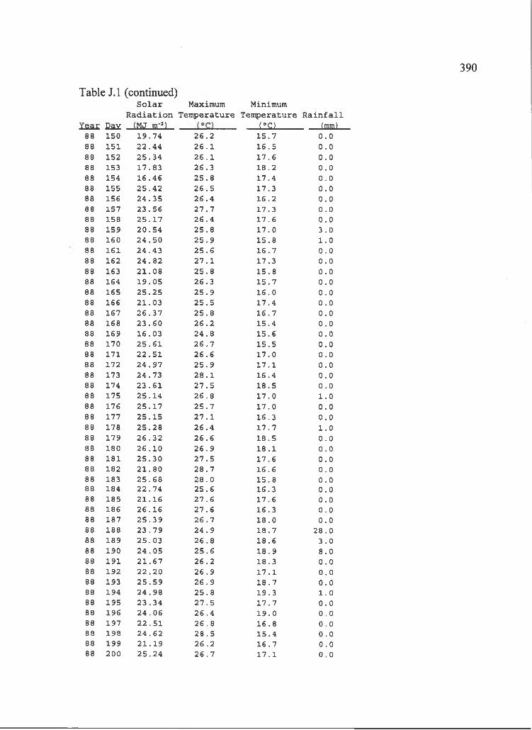
390
l a a c g a y IMJ m-')__________________ L isn______(mm)88 150 1 9 .7 4 2 6 . 2 1 5 . 7 0 . 088 151 2 2 . 4 4 2 6 . 1 1 6 . 5 0 . 088 152 2 5 . 3 4 2 6 . 1 1 7 . 6 0 . 088 153 1 7 .8 3 2 6 . 3 1 8 . 2 0 . 088 154 1 6 . 4 6 2 5 . 8 1 7 . 4 0 . 088 155 2 5 . 4 2 2 6 . 5 1 7 .3 0 . 088 156 2 4 . 3 5 2 6 . 4 1 6 . 2 0 . 088 157 2 3 . 5 6 2 7 . 7 1 7 .3 0 . 088 158 2 5 . 1 7 2 6 . 4 1 7 . 6 0 . 088 159 2 0 . 5 4 2 5 . 8 1 7 . 0 3 . 088 160 2 4 . 5 0 2 5 . 9 1 5 . 8 1 . 088 161 2 4 . 4 3 2 5 . 6 1 6 . 7 0 . 088 162 2 4 . 8 2 2 7 . 1 1 7 .3 0 . 088 163 2 1 . 0 8 2 5 . 8 1 5 . 8 0 . 088 164 1 9 . 0 5 2 6 . 3 1 5 . 7 0 . 088 165 2 5 . 2 5 2 5 . 9 1 6 . 0 0 . 088 166 2 1 . 0 3 2 5 . 5 1 7 .4 0 . 088 167 2 6 . 3 7 2 5 . 8 1 6 . 7 0 . 088 168 2 3 . 6 0 2 6 . 2 1 5 .4 0 . 088 169 1 6 . 0 3 2 4 . 8 1 5 . 6 0 . 088 170 2 5 . 6 1 2 6 . 7 1 5 . 5 0 . 088 171 2 2 . 5 1 2 6 . 6 1 7 . 0 0 . 088 172 2 4 . 9 7 2 5 . 9 1 7 . 1 0 . 088 173 2 4 . 7 3 2 8 . 1 1 6 .4 0 . 088 174 2 3 . 6 1 2 7 . 5 1 8 . 5 0 . 088 175 2 5 . 1 4 2 6 . 8 1 7 . 0 1 . 088 176 2 5 . 1 7 2 5 . 7 1 7 . 0 0 . 088 177 2 5 . 1 5 2 7 . 1 1 6 .3 0 . 088 178 2 5 . 2 8 2 6 . 4 1 7 . 7 1 . 088 179 2 6 . 3 2 2 6 . 6 1 8 . 5 0 . 088 180 2 6 . 1 0 2 6 . 9 1 8 . 1 0 . 088 181 2 5 . 3 0 2 7 . 5 1 7 . 6 0 . 088 182 2 1 . 8 0 2 8 . 7 1 6 . 6 0 . 088 183 2 5 . 6 8 2 8 . 0 1 5 . 8 0 . 088 184 2 2 . 7 4 2 5 . 6 1 6 .3 0 . 088 185 2 1 . 1 6 2 7 . 6 1 7 . 6 0 . 088 186 2 6 . 1 6 2 7 . 6 1 6 .3 0 . 088 187 2 5 . 3 9 2 6 . 7 1 8 . 0 0 . 088 188 2 3 . 7 9 2 4 . 9 1 8 . 7 2 8 . 088 189 2 5 . 0 3 2 6 . 8 1 8 .6 3 . 088 190 2 4 . 0 5 2 5 . 6 1 8 . 9 8 . 088 191 2 1 . 6 7 2 6 . 2 1 8 .3 0 . 088 192 2 2 . 2 0 2 6 . 9 1 7 . 1 0 . 088 193 2 5 . 5 9 2 6 . 9 1 8 . 7 0 . 088 194 2 4 . 9 8 2 5 . 8 1 9 .3 1 . 088 195 2 3 . 3 4 2 7 . 5 1 7 . 7 0 . 088 196 2 4 . 0 6 2 6 . 4 1 9 . 0 0 . 088 197 2 2 . 5 1 2 6 . 8 1 6 .8 0 . 088 198 2 4 . 6 2 2 8 . 5 1 5 .4 0 . 088 199 2 1 . 1 9 2 6 . 2 1 6 . 7 0 . 088 200 2 5 . 2 4 2 6 . 7 1 7 . 1 0 . 0
Table J.l (continued)S o l a r Maximum Minimum
R a d i a t i o n T e m p e r a tu r e T e m p e r a tu r e R a i n f a l l
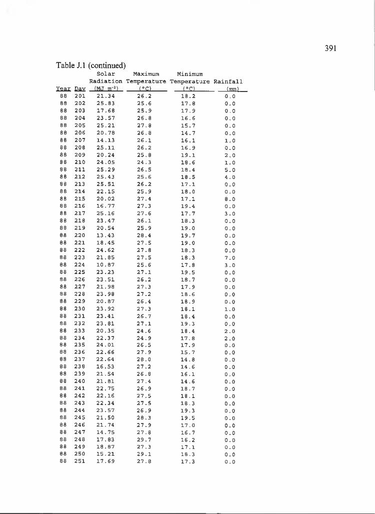
391
X s a r D a x ________L isn______ (mm)88 201 2 1 . 3 4 2 6 . 2 1 8 . 2 0 . 088 202 2 5 . 8 3 2 5 . 6 1 7 . 8 0 . 088 203 1 7 . 6 8 2 5 . 9 1 7 . 9 0 . 088 204 2 3 . 5 7 2 6 . 8 1 6 . 6 0 . 088 205 2 5 . 2 1 2 7 . 8 1 5 . 7 0 . 088 206 2 0 . 7 8 2 6 . 8 1 4 . 7 0 . 088 207 1 4 .1 3 2 6 . 1 1 6 . 1 1 . 088 208 2 5 . 1 1 2 6 . 2 1 6 . 9 0 . 088 209 2 0 . 2 4 2 5 . 8 1 9 . 1 2 . 088 210 2 4 . 0 5 2 4 . 3 1 8 . 6 1 . 088 211 2 5 . 2 9 2 6 . 5 1 8 . 4 5 . 088 212 2 5 . 4 3 2 5 . 6 1 8 . 5 4 . 088 213 2 5 . 5 1 2 6 . 2 1 7 . 1 0 . 088 214 2 2 . 1 5 2 5 . 9 1 8 . 0 0 . 088 215 2 0 . 0 2 2 7 . 4 1 7 . 1 8 . 088 216 1 6 . 7 7 2 7 . 3 1 9 . 4 0 . 088 217 2 5 . 1 6 2 7 . 6 1 7 . 7 3 . 088 218 2 3 . 4 7 2 6 . 1 1 8 .3 0 . 088 219 2 0 . 5 4 2 5 . 9 1 9 . 0 0 . 088 220 1 3 .4 3 2 8 . 4 1 9 . 7 0 . 088 221 1 8 . 4 5 2 7 . 5 1 9 . 0 0 . 088 222 2 4 . 6 2 2 7 . 8 1 8 .3 0 . 088 223 2 1 . 8 5 2 7 . 5 1 8 . 3 7 . 088 224 1 0 . 8 7 2 5 . 6 1 7 . 8 3 . 088 225 2 3 . 2 3 2 7 . 1 1 9 . 5 0 . 088 226 2 3 . 5 1 2 6 . 2 1 8 . 7 0 . 088 227 2 1 . 9 8 2 7 . 3 1 7 . 9 0 . 088 228 2 3 . 9 8 2 7 . 2 1 8 . 6 0 . 088 229 2 0 . 8 7 2 6 . 4 1 8 . 9 0 . 088 230 2 3 . 9 2 2 7 . 3 1 8 . 1 1 . 088 231 2 3 . 4 1 2 6 . 7 1 8 . 4 0 . 088 232 2 3 . 8 1 2 7 . 1 1 9 .3 0 . 088 233 2 0 . 3 5 2 4 . 6 1 8 .4 2 . 088 234 2 2 . 3 7 2 4 . 9 1 7 . 8 2 . 088 235 2 4 . 0 1 2 6 . 5 1 7 . 9 0 . 088 236 2 2 . 6 6 2 7 . 9 1 5 . 7 0 . 088 237 2 2 . 6 4 2 8 . 0 1 4 . 8 0 . 088 238 1 6 .5 3 2 7 . 2 1 4 . 6 0 . 088 239 2 1 . 5 4 2 6 . 8 1 6 . 1 0 . 088 240 2 1 . 8 1 2 7 . 4 1 4 . 6 0 . 088 241 2 2 . 7 5 2 6 . 9 1 8 . 7 0 . 088 242 2 2 . 1 6 2 7 . 5 1 8 . 1 0 . 088 243 2 2 . 3 4 2 7 . 5 1 8 .3 0 . 088 244 2 3 . 5 7 2 6 . 9 1 9 .3 0 . 088 245 2 1 . 5 0 2 8 . 3 1 9 . 5 0 . 088 246 2 1 . 7 4 2 7 . 9 1 7 . 0 0 . 088 247 1 4 . 7 5 2 7 . 8 1 6 . 7 0 . 088 248 1 7 .8 3 2 9 . 7 1 6 .2 0 . 088 249 1 8 . 8 7 2 7 . 3 1 7 . 1 0 . 088 250 1 5 . 2 1 2 9 . 1 1 8 .3 0 . 088 251 1 7 . 6 9 2 7 . 8 1 7 .3 0 . 0
Table J.l (continued)S o l a r Maximum Minimum
R a d i a t i o n T e m p e r a tu r e T e m p e ra tu r e R a i n f a l l

392
Xaa£ Eay (MJ _____ LI5U____ __Lisn________ (mm)88 252 2 2 . 2 3 2 7 . 6 1 6 . 9 0 . 088 253 1 1 . 6 0 2 7 . 5 1 5 . 9 0 . 088 254 1 0 . 7 5 2 5 . 5 1 6 .3 3 . 088 255 1 3 . 6 6 2 5 . 0 1 6 . 9 0 . 088 256 2 0 . 7 3 2 6 . 9 1 5 .3 0 . 088 257 1 9 . 4 7 2 7 . 4 1 6 .3 0 . 088 258 1 5 . 5 3 2 7 . 3 1 5 . 4 0 . 088 259 1 6 . 3 5 2 9 . 0 1 7 . 3 0 . 088 260 1 9 . 4 7 2 7 . 4 1 7 . 4 0 . 088 261 2 2 . 3 3 2 8 . 6 1 8 . 7 0 . 088 262 1 9 . 5 7 2 6 . 3 1 8 .3 3 . 088 263 2 0 . 8 1 2 7 . 6 1 8 . 0 0 . 088 264 1 8 . 3 1 2 5 . 6 1 8 . 5 1 . 088 265 2 1 . 2 4 2 6 . 2 1 8 . 3 1 . 088 266 2 1 . 5 8 2 6 . 5 1 8 . 5 5 . 088 267 1 8 .4 3 2 5 . 7 1 8 .3 4 . 088 268 1 7 . 6 7 2 6 . 0 1 7 . 7 0 . 088 269 1 7 . 6 5 2 6 . 6 1 6 . 8 0 . 088 270 1 6 . 0 9 2 8 . 2 1 8 . 1 1 1 . 088 271 1 3 . 3 0 2 8 . 4 1 8 .4 5 . 088 272 1 3 . 9 9 2 6 . 2 1 8 .3 0 . 088 273 1 5 . 7 7 2 7 . 9 1 7 . 5 0 . 088 274 2 0 . 4 4 3 0 . 2 1 6 . 7 0 . 088 275 2 0 . 3 0 3 0 . 0 1 5 . 5 0 . 088 276 1 8 . 2 8 2 9 . 6 1 5 . 1 0 . 088 277 1 7 . 6 4 2 8 . 2 1 5 . 1 0 . 088 278 1 6 . 5 5 2 9 . 6 1 4 . 7 0 . 088 279 1 9 . 8 1 2 6 . 5 1 6 . 9 0 . 088 280 1 7 . 6 3 2 5 . 8 1 8 . 1 0 . 088 281 1 8 . 2 8 2 6 . 0 1 9 .3 1 . 088 282 1 7 . 5 6 2 8 . 0 1 7 . 5 0 . 088 283 1 3 . 9 1 2 7 . 8 1 6 .4 0 . 088 284 1 4 .1 3 2 7 . 9 1 5 .4 0 . 088 285 1 5 . 7 7 2 7 . 6 1 6 . 5 0 . 088 286 1 6 .0 3 2 7 . 6 1 8 .3 1 8 .088 287 1 8 .6 3 2 7 . 0 1 9 . 1 0 . 088 288 1 3 . 0 0 2 7 . 0 1 6 . 9 0 . 088 289 1 2 . 2 0 2 7 . 4 1 6 . 7 0 . 088 290 1 0 . 2 2 2 5 . 7 1 7 . 9 1 .088 291 1 1 . 0 4 2 1 . 1 1 7 . 3 0 . 088 292 9 . 6 7 2 3 . 5 1 7 . 0 0 . 088 293 1 0 . 0 6 2 3 . 3 1 7 . 0 0 . 088 294 1 4 .0 3 2 6 . 6 1 5 . 6 0 . 088 295 1 4 . 3 0 2 5 . 4 1 7 . 2 0 . 088 296 1 1 . 9 0 2 7 . 9 1 6 . 2 0 . 088 297 7 . 5 8 2 7 . 8 1 6 . 4 3 . 088 298 9 . 7 0 2 6 . 7 1 6 .2 2 7 . 088 299 1 2 . 1 9 2 5 . 3 1 5 . 2 0 . 088 300 8 . 9 3 2 3 . 8 1 7 .4 1 . 088 301 1 2 . 6 2 2 5 . 1 1 7 .4 0 .088 302 1 1 . 0 9 2 4 . 9 1 7 .4 0 . 0
Table J. 1 (continued)S o l a r Maximum Minimum
R a d i a t i o n T e m p e r a tu r e T e m p e ra tu r e R a i n f a l l
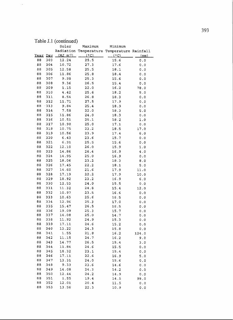
393
I s a x e a y (MJ ________tiil]______ L isn__________ (mm)88 303 1 2 . 2 4 2 5 . 5 1 5 . 6 0 . 088 304 1 0 . 7 2 2 7 . 3 1 7 . 6 0 . 088 305 1 2 . 5 8 2 5 . 5 1 8 . 1 0 . 088 306 1 1 . 8 6 2 5 . 8 1 8 . 4 0 . 088 307 9 . 9 8 2 5 . 3 1 5 . 6 0 . 088 308 9 . 3 6 2 6 . 5 1 5 . 4 0 . 088 309 1 . 1 5 2 2 . 0 1 6 . 2 7 8 . 088 310 4 . 4 2 2 5 . 6 1 8 . 2 5 . 088 311 8 . 5 4 2 6 . 8 1 8 .3 0 . 088 312 1 1 . 7 1 2 7 . 5 1 7 . 9 0 . 088 313 9 . 8 4 2 5 . 4 1 8 . 9 0 . 088 314 7 . 5 8 2 2 . 0 1 8 .3 5 . 088 315 1 1 . 8 6 2 4 . 0 1 8 .3 0 . 088 316 1 0 . 5 1 2 5 . 1 1 8 . 2 1 . 088 317 1 0 . 9 0 2 5 . 0 1 7 . 1 0 . 088 318 1 0 . 7 5 2 3 . 2 1 8 . 5 1 7 .088 319 1 0 . 5 6 2 3 . 9 1 7 . 4 6 . 088 320 6 . 4 3 2 3 . 6 1 5 . 7 0 . 088 321 6 . 9 1 2 5 . 5 1 5 . 6 0 . 088 322 1 2 . 1 0 2 6 . 0 1 5 . 9 1 .088 323 1 4 . 8 6 2 6 . 4 1 6 . 9 4 . 088 324 1 4 . 9 5 2 5 . 0 1 6 . 9 0 . 088 325 1 8 . 0 6 2 3 . 2 1 8 .3 8 . 088 326 1 7 . 4 5 2 2 . 2 1 8 . 1 5 . 088 327 1 4 . 6 0 2 1 . 6 1 7 . 9 1 1 .088 328 1 7 . 1 9 2 2 . 2 1 7 . 9 1 0 .088 329 1 8 . 9 2 2 3 . 2 1 6 . 9 6 . 088 330 1 2 .5 3 2 4 . 0 1 5 . 5 0 . 088 331 1 1 . 3 2 2 4 . 8 1 5 . 4 1 2 .088 332 1 0 . 9 7 2 3 . 5 1 6 . 6 0 . 088 333 1 0 .6 3 2 5 . 6 1 6 . 5 0 . 088 334 1 2 . 9 6 2 5 . 3 1 7 . 0 0 . 088 335 1 5 . 4 7 2 6 . 5 1 6 . 5 0 . 088 336 1 9 . 0 9 2 5 . 3 1 5 . 7 0 . 088 337 1 4 . 0 8 2 5 . 0 1 4 . 7 0 . 088 338 1 1 . 9 2 2 4 . 9 1 5 .3 0 . 088 339 1 7 . 1 1 2 4 . 6 1 5 . 2 0 . 088 340 1 3 . 2 2 2 4 . 3 1 5 . 8 0 . 088 341 1 . 5 5 2 1 . 8 1 6 . 2 1 2 4 .088 342 1 1 . 1 5 2 4 . 7 1 6 .2 9 . 088 343 1 4 . 7 7 2 6 . 5 1 5 . 4 3 . 088 344 1 1 . 8 4 2 4 . 6 1 5 . 5 0 . 088 345 1 8 . 3 2 2 3 . 1 1 5 .4 0 . 088 346 1 7 . 1 1 2 2 . 6 1 6 . 9 5 . 088 347 1 3 . 3 1 2 4 . 0 1 5 . 6 0 . 088 348 9 . 3 3 2 3 . 6 1 4 . 6 0 . 088 349 1 4 . 0 8 2 4 . 3 1 4 . 2 0 . 088 350 1 2 .4 4 2 4 . 2 1 4 . 9 0 . 088 351 1 . 5 5 1 9 . 4 1 4 . 5 9 8 . 088 352 1 2 . 0 1 2 0 . 4 1 1 . 5 0 . 088 353 1 3 . 5 6 2 2 . 3 1 0 . 9 0 . 0
Table J.l (continued)S o l a r Maximum Minimum
R a d i a t i o n T e m p e r a tu r e T e m p e r a tu r e R a i n f a l l
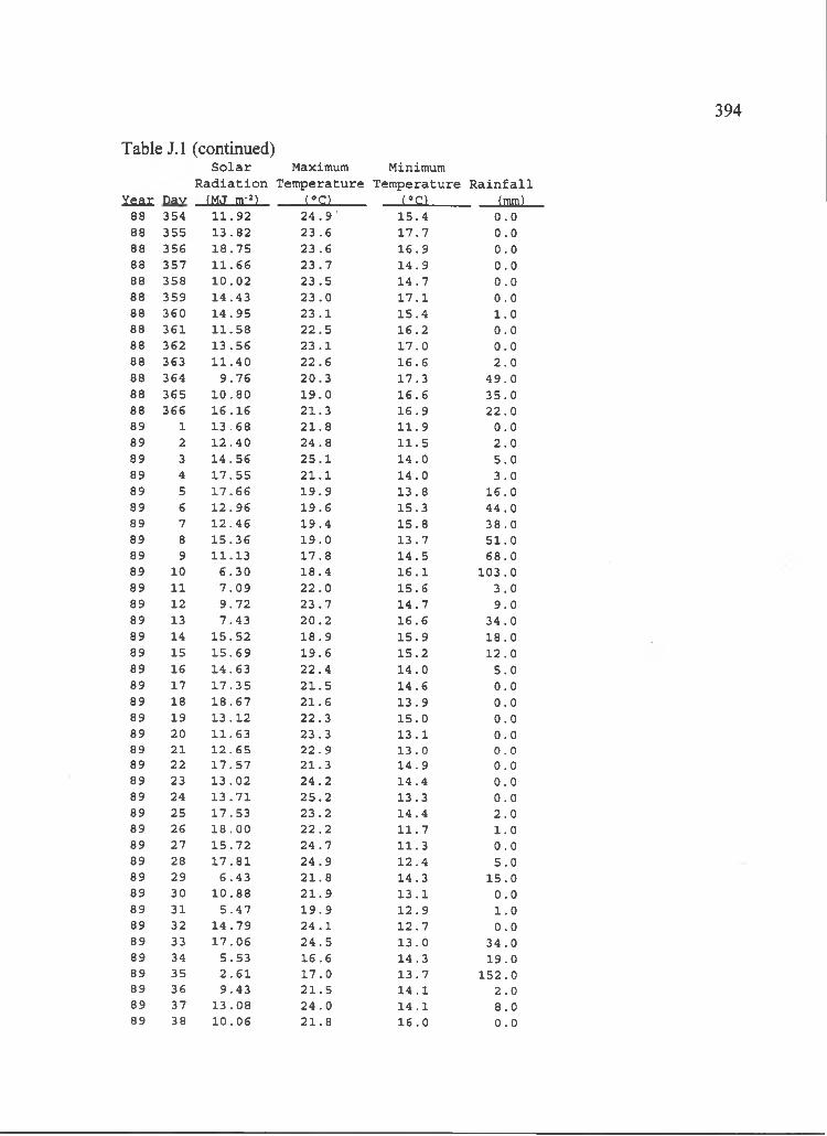
394
Yea r Dav (MJ m' )________ LlSn_____ (°C)____________(mm)88 354 1 1 . 9 2 2 4 . 9 ’ 1 5 .4 0 . 088 355 1 3 . 8 2 2 3 . 6 1 7 . 7 0 . 088 356 1 8 . 7 5 2 3 . 6 1 6 . 9 0 . 088 357 1 1 . 6 6 2 3 . 7 1 4 . 9 0 . 088 358 1 0 . 0 2 2 3 . 5 1 4 . 7 0 . 088 359 1 4 .4 3 2 3 . 0 1 7 . 1 0 . 088 360 1 4 . 9 5 2 3 . 1 1 5 . 4 1 . 088 361 1 1 . 5 8 2 2 . 5 1 6 . 2 0 . 088 362 1 3 . 5 6 2 3 . 1 1 7 . 0 0 . 088 363 1 1 . 4 0 2 2 . 6 1 6 . 6 2 . 088 364 9 . 7 6 2 0 . 3 1 7 .3 4 9 . 088 365 1 0 . 8 0 1 9 . 0 1 6 . 6 3 5 . 088 366 1 6 . 1 6 2 1 . 3 1 6 . 9 2 2 . 089 1 1 3 . 6 8 2 1 . 8 1 1 . 9 0 . 089 2 1 2 . 4 0 2 4 . 8 1 1 . 5 2 . 089 3 1 4 . 5 6 2 5 . 1 1 4 . 0 5 . 089 4 1 7 . 5 5 2 1 . 1 1 4 . 0 3 . 089 5 1 7 . 6 6 1 9 . 9 1 3 . 8 1 6 . 089 6 1 2 . 9 6 1 9 . 6 1 5 .3 4 4 . 089 7 1 2 . 4 6 1 9 . 4 1 5 . 8 3 8 . 089 8 1 5 . 3 6 1 9 . 0 1 3 . 7 5 1 . 089 9 1 1 .1 3 1 7 . 8 1 4 . 5 6 8 . 089 10 6 . 3 0 1 8 . 4 1 6 . 1 1 0 3 .089 11 7 . 0 9 2 2 . 0 1 5 . 6 3 . 089 12 9 . 7 2 2 3 . 7 1 4 . 7 9 . 089 13 7 . 4 3 2 0 . 2 1 6 . 6 3 4 . 089 14 1 5 . 5 2 1 8 . 9 1 5 . 9 1 8 . 089 15 1 5 . 6 9 1 9 . 6 1 5 . 2 1 2 . 089 16 1 4 .6 3 2 2 . 4 1 4 . 0 5 . 089 17 1 7 . 3 5 2 1 . 5 1 4 .6 0 . 089 18 1 8 . 6 7 2 1 . 6 1 3 . 9 0 . 089 19 1 3 . 1 2 2 2 . 3 1 5 . 0 0 . 089 20 1 1 .6 3 2 3 . 3 1 3 . 1 0 . 089 21 1 2 . 6 5 2 2 . 9 1 3 . 0 0 . 089 22 1 7 . 5 7 2 1 . 3 1 4 . 9 0 . 089 23 1 3 . 0 2 2 4 . 2 1 4 . 4 0 . 089 24 1 3 . 7 1 2 5 . 2 1 3 . 3 0 . 089 25 1 7 .5 3 2 3 . 2 1 4 .4 2 . 089 26 1 8 . 0 0 2 2 . 2 1 1 . 7 1 . 089 27 1 5 . 7 2 2 4 . 7 1 1 .3 0 . 089 28 1 7 . 8 1 2 4 . 9 1 2 . 4 5 . 089 29 6 . 4 3 2 1 . 8 1 4 .3 1 5 . 089 30 1 0 . 8 8 2 1 . 9 1 3 . 1 0 . 089 31 5 . 4 7 1 9 . 9 1 2 . 9 1 . 089 32 1 4 . 7 9 2 4 . 1 1 2 . 7 0 . 089 33 1 7 . 0 6 2 4 . 5 1 3 . 0 3 4 . 089 34 5 . 5 3 1 6 . 6 1 4 .3 1 9 .089 35 2 . 6 1 1 7 . 0 1 3 . 7 15 2 .089 36 9 . 4 3 2 1 . 5 1 4 . 1 2 . 089 37 1 3 .0 8 2 4 . 0 1 4 . 1 8 .089 38 1 0 . 0 6 2 1 . 8 1 6 . 0 0 . 0
Table J.l (continued)S o l a r Maximum Minimum
R a d i a t i o n T e m p e r a tu r e T e m p e ra tu r e R a i n f a l l
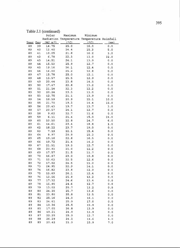
395
Year Bay Lisn_ _____ (mm)89 39 1 4 . 7 5 2 5 . 0 1 6 . 0 0 . 089 40 1 2 . 4 0 2 4 . 4 1 5 .3 5 . 089 41 1 0 . 0 5 2 1 . 8 1 6 . 2 3 . 089 42 6 . 7 8 2 2 . 3 1 3 . 0 3 2 . 089 43 1 4 . 5 1 2 4 . 1 1 3 . 9 0 . 089 44 1 5 .5 3 2 5 . 9 1 2 . 7 0 . 089 45 1 9 . 1 6 2 6 . 1 1 2 . 4 0 . 089 46 1 6 . 0 0 2 5 . 2 1 2 . 8 0 . 089 47 1 5 . 7 8 2 5 . 0 1 2 . 1 0 . 089 48 1 5 . 5 7 2 5 . 5 1 2 . 9 0 . 089 49 2 0 . 4 4 2 3 . 8 1 4 . 5 0 . 089 50 1 7 . 4 7 2 2 . 8 1 3 . 2 0 . 089 51 2 1 . 1 4 2 2 . 3 1 2 . 2 0 . 089 52 2 0 . 2 4 2 3 . 3 1 3 . 0 0 . 089 53 1 2 . 7 5 2 1 . 1 1 3 . 9 0 . 089 54 1 8 . 5 9 2 0 . 9 1 5 . 1 1 0 .089 55 2 1 . 7 0 1 9 . 3 1 4 . 4 1 5 .089 56 2 0 . 4 3 1 9 . 7 1 3 . 7 3 . 089 57 2 0 . 5 7 2 4 . 1 1 2 . 7 0 . 089 58 9 . 6 2 2 2 . 7 1 1 . 6 0 .089 59 6 . 1 1 2 1 . 4 1 5 . 0 2 1 . 089 60 1 0 . 5 0 2 2 . 8 1 4 . 7 6 . 089 61 1 4 . 6 1 2 3 . 4 1 8 . 8 1 . 089 62 1 8 . 2 2 2 3 . 7 1 9 . 0 0 . 089 63 7 . 1 9 2 2 . 1 1 5 . 4 0 . 089 64 8 . 9 7 2 0 . 9 1 5 .3 0 . 089 65 1 9 . 1 6 2 2 . 8 1 6 . 5 0 . 089 66 1 9 . 7 2 2 1 . 4 1 4 . 2 0 . 089 67 2 1 . 5 1 1 9 . 3 1 2 . 7 0 . 089 68 2 0 . 9 3 2 1 . 0 1 2 . 2 0 . 089 69 1 7 . 5 7 2 1 . 5 1 1 . 7 0 . 089 70 1 6 . 8 7 2 3 . 0 1 0 . 8 0 . 089 71 1 5 .6 3 2 2 . 5 1 2 . 6 0 . 089 72 1 7 . 0 2 2 4 . 5 1 1 . 0 0 . 089 73 2 4 . 9 5 2 2 . 9 1 4 . 1 0 . 089 74 1 6 . 8 2 2 3 . 8 1 2 . 9 0 . 089 75 1 5 . 6 9 2 6 . 1 1 2 . 4 0 . 089 76 1 3 . 5 6 2 5 . 8 1 3 . 2 0 . 089 77 1 7 . 3 2 2 4 . 6 1 3 .4 0 . 089 78 1 5 . 9 0 2 4 . 6 1 2 . 7 0 . 089 79 1 3 . 0 2 2 5 . 7 1 3 . 2 0 . 089 80 2 4 . 3 0 2 5 . 7 1 3 . 6 0 . 089 81 2 3 . 8 0 2 5 . 8 1 3 . 5 0 . 089 82 2 5 . 1 6 2 4 . 3 1 6 . 1 0 . 089 83 2 4 . 6 1 2 5 . 9 1 7 . 0 0 . 089 84 1 0 . 3 6 2 5 . 5 1 5 . 9 0 . 089 85 1 7 . 0 5 2 6 . 8 1 3 . 9 0 . 089 86 1 9 . 2 1 2 4 . 9 1 3 . 9 0 . 089 87 2 2 . 2 5 2 5 . 9 1 3 . 7 0 .089 88 2 6 . 2 9 2 4 . 3 1 4 . 6 1 . 089 89 2 0 . 4 2 2 1 . 9 1 5 . 9 7 . 0
Table J.l (continued)S o l a r Maximum Minimum
R a d i a t i o n T e m p e r a tu r e T e m p e r a tu r e R a i n f a l l
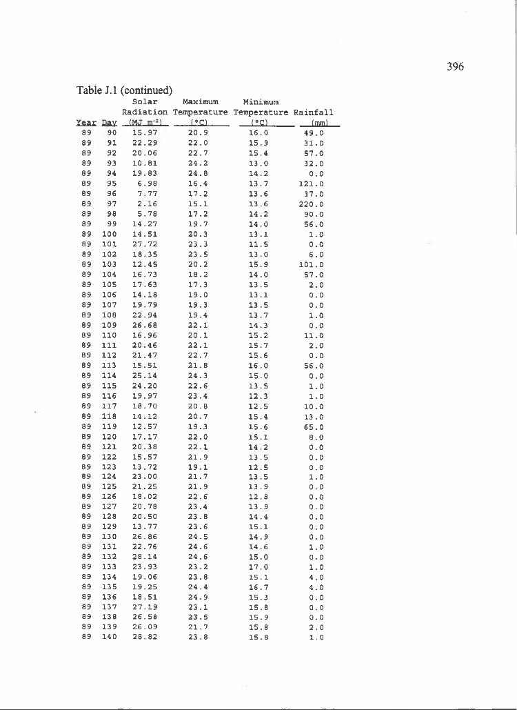
396
Table J.l (continued)S o l a r Maximum Minimum
R a d i a t i o n Temperatur e Temperature R a i n f a l l Y e a r I > a x ( M J ilSl L l i l l ______________ (mm)
89 90 1 5 . 9 7 2 0 . 9 1 6 .0 4 9 . 089 91 2 2 . 2 9 2 2 . 0 1 5 .9 3 1 . 089 92 2 0 . 0 6 2 2 . 7 1 5 .4 5 7 . 089 93 1 0 . 8 1 24 .2 1 3 .0 3 2 . 089 94 19 .8 3 2 4 . 8 1 4 .2 0 . 089 95 6 . 9 8 16 .4 1 3 . 7 1 2 1 .089 96 7 . 7 7 1 7 . 2 1 3 .6 3 7 . 089 97 2 . 1 6 1 5 . 1 13 .6 2 2 0 . 089 98 5 . 7 8 1 7 .2 1 4 .2 9 0 . 089 99 14 .27 1 9 . 7 1 4 .0 56 .089 100 14 .51 2 0 . 3 1 3 . 1 1 . 089 101 2 7 . 7 2 23 .3 1 1 .5 0 . 089 102 1 8 . 3 5 2 3 . 5 1 3 . 0 6 . 089 103 1 2 .4 5 2 0 . 2 1 5 .9 1 0 1 .089 104 1 6 .7 3 1 8 . 2 1 4 .0 5 7 . 089 105 1 7 .6 3 1 7 .3 13 .5 2 . 089 106 1 4 . 1 8 1 9 . 0 1 3 .1 0 . 089 107 1 9 . 7 9 1 9 .3 1 3 . 5 0 . 089 108 2 2 . 9 4 1 9 . 4 1 3 . 7 1 . 089 109 2 6 . 6 8 2 2 . 1 14 .3 0 . 089 110 1 6 .9 6 2 0 . 1 1 5 . 2 1 1 . 089 111 2 0 . 4 6 2 2 . 1 1 5 . 7 2 . 089 112 2 1 . 4 7 2 2 . 7 1 5 . 6 0 . 089 113 1 5 . 5 1 21 . 8 1 6 . 0 5 6 . 089 114 2 5 . 1 4 2 4 . 3 1 5 . 0 0 . 089 115 2 4 . 2 0 2 2 . 6 1 3 . 5 1 . 089 116 1 9 . 9 7 2 3 . 4 12 .3 1 . 089 117 1 8 .7 0 2 0 . 8 1 2 . 5 10 .089 118 1 4 .1 2 2 0 . 7 1 5 .4 13 .089 119 1 2 . 5 7 1 9 .3 1 5 .6 6 5 . 089 120 1 7 . 1 7 2 2 . 0 1 5 . 1 8 .089 121 2 0 . 3 8 2 2 . 1 1 4 .2 0 . 089 122 1 5 . 5 7 2 1 . 9 1 3 . 5 0 . 089 123 13 .72 1 9 . 1 1 2 . 5 0 . 089 124 2 3 . 0 0 2 1 . 7 1 3 . 5 1 .089 125 2 1 . 2 5 2 1 . 9 13 .9 0 . 089 126 1 8 .0 2 2 2 . 6 1 2 .8 0 . 089 127 2 0 . 7 8 2 3 . 4 1 3 . 9 0 . 089 128 2 0 . 5 0 23 .8 1 4 .4 0 . 089 129 13 .77 23 .6 1 5 .1 0 . 089 130 2 6 . 8 6 24 .5 1 4 .9 0 . 089 131 2 2 . 7 6 2 4 . 6 1 4 .6 1 . 089 132 2 8 . 1 4 2 4 . 6 1 5 .0 0 . 089 133 23 .93 23 .2 1 7 .0 1 . 089 134 1 9 .0 6 23 .8 1 5 . 1 4 . 089 135 1 9 . 2 5 24 .4 1 6 . 7 4 . 089 136 1 8 . 5 1 2 4 . 9 1 5 .3 0 . 089 137 2 7 . 1 9 2 3 . 1 1 5 .8 0 . 089 138 2 6 . 5 8 23 .5 1 5 . 9 0 . 089 139 2 6 . 0 9 2 1 . 7 15 .8 2 . 089 140 2 8 . 8 2 23 .8 1 5 .8 1 . 0
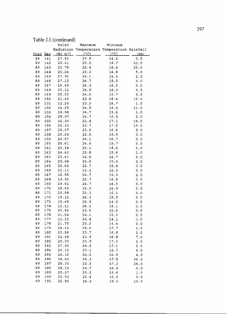
397
Table J.l (continued)S o l a r Maximum Minimum
R a d i a t i o n Temperat ure Temperature R a i n f a l lY ea r Day (MJ m' )__________________________________ (mm)
89 141 2 7 . 5 3 2 3 . 8 1 4 . 2 0 . 089 142 2 0 . 4 1 2 3 . 2 1 6 . 7 2 3 . 089 143 2 3 . 7 8 2 2 . 4 1 6 . 4 2 0 . 089 144 2 5 . 2 4 2 3 . 3 1 6 . 8 5 . 089 145 2 7 . 9 3 2 4 . 1 1 6 . 4 2 . 089 146 2 7 . 1 2 2 6 . 7 1 5 . 5 0 . 089 147 1 6 . 4 9 2 6 . 9 1 6 .3 0 . 089 148 2 5 . 1 2 2 5 . 9 1 8 . 0 0 . 089 149 2 5 . 0 3 2 4 . 0 1 6 . 7 4 . 089 150 2 1 . 4 3 2 2 . 6 1 6 . 4 1 2 .089 151 1 2 . 2 0 2 3 . 3 1 6 . 7 1 . 089 152 1 4 . 2 9 2 4 . 5 1 5 . 4 1 1 .089 153 1 9 . 9 8 2 4 . 7 1 3 . 6 1 . 089 154 2 8 . 9 7 2 4 . 7 1 6 . 5 2 . 089 155 1 6 . 3 0 2 1 . 8 1 7 . 1 1 6 .089 156 2 6 . 2 3 2 3 . 7 1 7 . 2 1 9 .089 157 2 8 . 0 7 2 3 . 2 1 6 . 6 5 . 089 158 2 0 . 2 4 2 2 . 5 1 5 . 9 2 . 089 159 2 0 . 5 7 2 4 . 1 1 6 . 7 0 . 089 160 2 8 . 6 1 2 4 . 4 1 5 . 7 0 . 089 161 2 3 . 1 8 2 3 . 1 1 5 . 6 0 . 089 162 2 4 . 6 2 2 3 . 8 1 5 . 6 1 . 089 163 2 3 . 4 1 2 2 . 5 1 6 . 7 3 . 089 164 2 9 . 4 8 2 4 . 6 1 5 . 5 2 . 089 165 2 5 . 6 0 2 2 . 7 1 5 . 4 3 . 089 166 2 2 . 1 1 2 3 . 1 1 6 . 3 0 . 089 167 1 8 . 5 5 2 4 . 7 1 5 . 9 2 . 089 168 1 9 .9 3 2 2 . 7 1 6 . 8 3 . 089 169 2 9 . 8 2 2 4 . 7 1 6 .3 0 . 089 170 2 8 . 2 0 2 5 . 2 1 6 . 9 0 . 089 171 2 0 . 0 8 2 3 . 3 1 6 . 1 1 . 089 172 1 9 . 1 2 2 6 . 1 1 5 . 9 0 . 089 173 1 5 . 4 5 2 6 . 9 1 4 . 0 0 . 089 174 1 5 . 1 1 2 6 . 1 1 5 . 1 0 . 089 175 2 6 . 8 6 2 5 . 6 1 5 . 5 0 . 089 176 2 1 . 0 4 2 4 . 1 1 5 .3 0 . 089 177 1 5 . 3 2 2 5 . 4 1 4 . 1 1 . 089 178 2 1 . 7 5 2 5 . 3 1 4 . 4 0 . 089 179 2 8 . 1 2 2 5 . 1 1 7 . 7 1 . 089 180 2 3 . 5 6 2 3 . 7 1 6 . 8 2 . 089 181 2 2 . 4 8 2 3 . 9 1 6 . 8 7 . 089 182 2 9 . 3 0 2 3 . 9 1 7 . 0 1 . 089 183 2 7 . 5 0 2 4 . 5 1 7 . 1 0 . 089 184 2 0 . 1 0 2 3 . 1 1 6 . 7 6 . 089 185 2 4 . 1 6 2 4 . 2 1 6 . 8 4 . 089 186 2 8 . 4 0 2 4 . 3 1 7 . 5 3 6 . 089 187 2 5 . 3 0 2 2 . 2 1 7 .3 2 4 . 089 188 2 8 . 1 3 2 4 . 7 1 6 . 5 0 . 089 189 2 5 . 2 7 2 5 . 2 1 5 . 6 1 . 089 190 2 3 . 5 3 2 5 . 4 1 6 . 0 0 . 089 191 2 2 . 8 0 2 4 . 2 1 8 .4 1 4 . 0
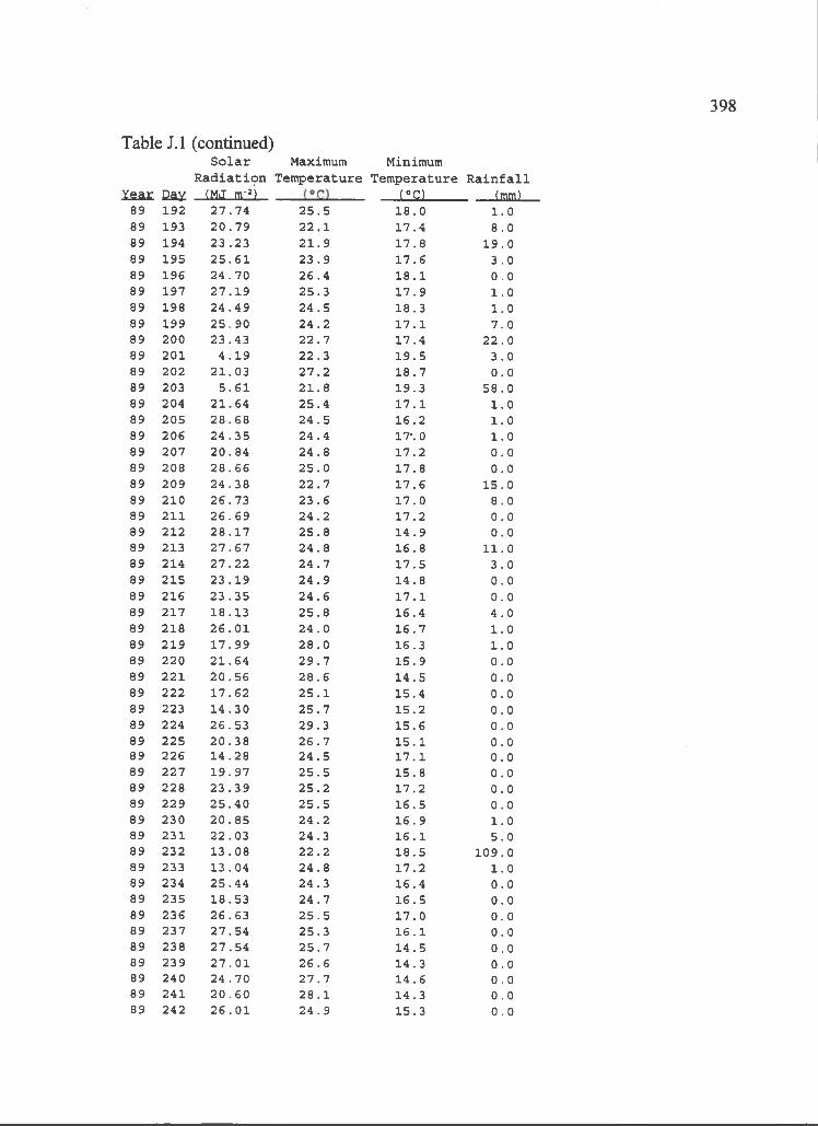
398
Year Eay ,tMJ m' i ____ (°o________ (mm)89 192 2 7 . 7 4 2 5 . 5 1 8 . 0 1 . 089 193 2 0 . 7 9 2 2 . 1 1 7 . 4 8 . 089 194 2 3 . 2 3 2 1 . 9 1 7 . 8 1 9 .089 195 2 5 . 6 1 2 3 . 9 1 7 . 6 3 . 089 196 2 4 . 7 0 2 6 . 4 1 8 . 1 0 . 089 197 2 7 . 1 9 2 5 . 3 1 7 . 9 1 . 089 198 2 4 . 4 9 2 4 . 5 1 8 .3 1 . 089 199 2 5 . 9 0 2 4 . 2 1 7 . 1 7 . 089 200 2 3 . 4 3 2 2 . 7 1 7 . 4 2 2 . 089 201 4 . 1 9 2 2 . 3 1 9 . 5 3 . 089 202 2 1 . 0 3 2 7 . 2 1 8 . 7 0 . 089 203 5 . 6 1 2 1 . 8 1 9 .3 5 8 . 089 204 2 1 . 6 4 2 5 . 4 1 7 . 1 1 . 089 205 2 8 . 6 8 2 4 . 5 1 6 . 2 1 . 089 206 2 4 . 3 5 2 4 . 4 17*. 0 1 . 089 207 2 0 . 8 4 2 4 . 8 1 7 . 2 0 . 089 208 2 8 . 6 6 2 5 . 0 1 7 . 8 0 . 089 209 2 4 . 3 8 2 2 . 7 1 7 . 6 1 5 . 089 210 2 6 . 7 3 2 3 . 6 1 7 . 0 8 . 089 211 2 6 . 6 9 2 4 . 2 1 7 . 2 0 . 089 212 2 8 . 1 7 2 5 . 8 1 4 . 9 0 . 089 213 2 7 . 6 7 2 4 . 8 1 6 . 8 1 1 . 089 214 2 7 . 2 2 2 4 . 7 1 7 . 5 3 . 089 215 2 3 . 1 9 2 4 . 9 1 4 . 8 0 . 089 216 2 3 . 3 5 2 4 . 6 1 7 . 1 0 . 089 217 1 8 .1 3 2 5 . 8 1 6 . 4 4 . 089 218 2 6 . 0 1 2 4 . 0 1 6 . 7 1 . 089 219 1 7 . 9 9 2 8 . 0 1 6 .3 1 . 089 220 2 1 . 6 4 2 9 . 7 1 5 . 9 0 . 089 221 2 0 . 5 6 2 8 . 6 1 4 . 5 0 . 089 222 1 7 . 6 2 2 5 . 1 1 5 . 4 0 . 089 223 1 4 . 3 0 2 5 . 7 1 5 . 2 0 . 089 224 2 6 . 5 3 2 9 . 3 1 5 . 6 0 . 089 225 2 0 . 3 8 2 6 . 7 1 5 . 1 0 . 089 226 1 4 . 2 8 2 4 . 5 1 7 . 1 0 . 089 227 1 9 . 9 7 2 5 . 5 1 5 . 8 0 . 089 228 2 3 . 3 9 2 5 . 2 1 7 . 2 0 . 089 229 2 5 . 4 0 2 5 . 5 1 6 . 5 0 . 089 230 2 0 . 8 5 2 4 . 2 1 6 . 9 1 . 089 231 2 2 . 0 3 2 4 . 3 1 6 . 1 5 . 089 232 1 3 . 0 8 2 2 . 2 1 8 . 5 1 0 9 .089 233 1 3 .0 4 2 4 . 8 1 7 . 2 1 . 089 234 2 5 . 4 4 2 4 . 3 1 6 . 4 0 . 089 235 1 8 .5 3 2 4 . 7 1 6 . 5 0 . 089 236 2 6 . 6 3 2 5 . 5 1 7 . 0 0 . 089 237 2 7 . 5 4 2 5 . 3 1 6 . 1 0 . 089 238 2 7 . 5 4 2 5 . 7 1 4 . 5 0 . 089 239 2 7 . 0 1 2 6 . 6 1 4 .3 0 . 089 240 2 4 . 7 0 2 7 . 7 1 4 . 6 0 . 089 241 2 0 . 6 0 2 8 . 1 1 4 .3 0 . 089 242 2 6 . 0 1 2 4 . 9 1 5 .3 0 . 0
Table J.l (continued)S o l a r Maximum Minimum
R a d i a t i o n T e m p e r a tu r e T e m p e r a tu r e R a i n f a l l
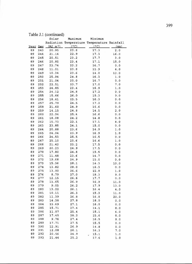
399
Table J.l (continued)S o l a r Maximum Minimum
R a d i a t i o n Temperat ure Temperature R a i n f a l lY ear Dav (MJ m~ )____________________________ (mm)
89 243 2 0 . 9 5 2 3 . 8 1 7 .3 2 . 089 244 2 1 . 1 4 2 2 . 9 1 7 .3 1 6 . 089 245 2 0 . 5 1 2 3 . 2 1 7 . 7 3 . 089 246 2 0 . 8 5 2 3 . 4 1 7 . 1 1 5 .089 247 2 3 . 7 4 2 3 . 2 1 6 . 7 0 . 089 248 1 1 . 0 1 2 3 . 8 1 5 . 9 4 . 089 249 1 0 .3 4 2 3 . 6 1 4 . 0 1 3 . 089 250 2 5 . 9 4 2 4 . 8 1 6 .3 1 . 089 251 2 1 . 0 4 2 5 . 0 1 6 . 7 0 . 089 252 2 2 . 5 1 2 3 . 7 1 7 . 0 7 . 089 253 2 4 . 8 5 2 3 . 4 1 6 . 9 1 . 089 254 2 4 . 1 2 2 4 . 8 1 7 . 2 0 . 089 255 1 5 . 6 6 2 6 . 0 1 5 .3 9 . 089 256 1 8 . 6 1 2 5 . 5 1 6 .3 0 . 089 257 2 5 . 7 9 2 4 . 5 1 7 . 2 0 . 089 258 2 1 . 6 0 2 4 . 9 1 6 . 6 0 . 089 259 1 4 . 1 5 2 4 . 8 1 4 . 5 2 . 089 260 2 2 . 9 4 2 5 . 4 1 6 . 6 0 . 089 261 1 8 . 0 8 2 4 . 2 1 4 . 8 0 . 089 262 1 5 .7 3 2 2 . 1 1 7 . 1 4 . 089 263 2 3 . 8 5 2 4 . 1 1 5 . 0 0 . 089 264 2 0 . 8 8 2 3 . 6 1 4 . 9 1 . 089 265 2 4 . 0 4 2 3 . 9 1 6 . 9 1 . 089 266 2 4 . 5 3 2 5 . 5 1 6 . 5 0 . 089 267 2 5 . 1 0 2 5 . 6 1 6 . 6 1 . 089 268 2 1 . 4 2 2 5 . 2 1 7 . 5 0 . 089 269 2 0 . 2 3 2 4 . 9 1 7 . 5 0 . 089 270 1 7 . 8 0 2 4 . 8 1 5 . 5 0 . 089 271 1 1 . 4 8 2 3 . 6 1 4 . 7 0 . 089 272 1 9 . 6 8 2 4 . 9 1 5 . 0 0 . 089 273 1 5 . 3 6 2 8 . 1 1 4 . 3 1 0 . 089 274 1 3 . 8 2 2 8 . 0 16 .3 0 . 089 275 1 3 . 9 0 2 6 . 6 1 5 . 9 1 . 089 276 8 . 7 9 2 7 . 0 1 8 .3 9 . 089 277 1 2 . 1 5 2 6 . 6 1 7 . 7 0 . 089 278 1 1 . 6 5 2 6 . 9 1 6 . 9 1 1 . 089 279 9 . 0 5 2 6 . 2 1 7 . 9 1 3 .089 280 1 3 . 2 2 2 6 . 1 1 6 . 4 4 . 089 281 1 0 . 1 1 2 6 . 3 1 5 .3 1 1 .089 282 1 1 . 3 9 2 6 . 8 1 6 . 8 2 0 . 089 283 1 4 . 3 8 2 7 . 8 1 8 . 0 0 . 089 284 1 5 . 6 9 2 7 . 1 1 6 . 0 0 . 089 285 1 5 . 7 1 2 7 . 4 1 4 . 1 0 . 089 286 1 1 . 0 7 2 5 . 4 1 5 . 1 6 . 089 287 1 7 . 4 5 2 8 . 2 1 5 . 6 0 . 089 288 9 . 7 6 2 7 . 4 1 6 . 5 8 . 089 289 1 7 . 7 1 2 7 . 5 1 5 . 5 0 . 089 290 1 2 . 9 1 2 6 . 9 1 4 . 8 0 .089 291 1 2 .0 8 2 6 . 1 1 6 .3 7 . 089 292 2 0 . 5 6 2 4 . 9 . 1 5 . 1 1 .089 293 2 1 . 4 4 2 5 . 2 1 7 . 6 1 . 0
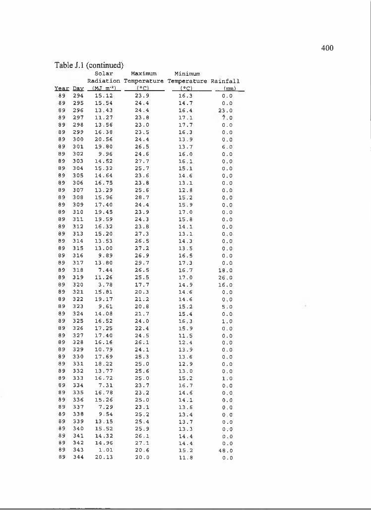
400
Table J.l (continued)S o l a r Maximum Minimum
R a d i a t i o n Tem peratur e Temperature R a i n f a l lY ear Dav (MJ m' -)__________________ (°C)______(mm)
89 294 1 5 . 1 2 2 3 . 9 1 6 .3 0 . 089 295 1 5 .5 4 2 4 . 4 1 4 . 7 0 . 089 296 1 3 .4 3 2 4 . 4 1 6 . 4 2 3 . 089 297 1 1 . 2 7 2 3 . 8 1 7 . 1 . 089 298 1 3 . 5 6 2 3 . 0 1 7 . 7 0 . 089 299 1 6 . 3 8 2 3 . 5 1 6 .3 0 . 089 300 2 0 . 5 6 2 4 . 4 1 3 . 9 0 . 089 301 1 9 . 8 0 2 6 . 5 1 3 . 7 6 . 089 302 9 . 9 6 2 4 . 6 1 6 . 0 0 . 089 303 1 4 . 5 2 2 7 . 7 1 6 . 1 0 . 089 304 1 5 . 3 2 2 5 . 7 1 5 . 1 0 . 089 305 1 4 . 6 4 2 3 . 6 1 4 . 6 0 . 089 306 1 6 . 7 5 2 3 . 8 1 3 . 1 0 . 089 307 1 3 . 2 9 2 5 . 6 1 2 . 8 0 . 089 308 1 5 . 9 6 2 8 . 7 1 5 . 2 0 . 089 309 1 7 . 4 0 2 4 . 4 1 5 . 9 0 . 089 310 1 9 . 4 5 2 3 . 9 1 7 . 0 0 . 089 311 1 9 . 5 9 2 4 . 3 1 5 . 8 0 . 089 312 1 6 . 3 2 2 3 . 8 1 4 . 1 0 . 089 313 1 5 . 2 0 2 7 . 3 1 3 . 1 0 . 089 314 1 3 .5 3 2 6 . 5 1 4 .3 0 . 089 315 1 3 . 0 0 2 7 . 2 1 3 . 5 0 . 089 316 9 . 8 9 2 6 . 9 1 6 . 5 0 . 089 317 1 3 . 8 0 2 9 . 7 1 7 .3 0 . 089 318 7 . 4 4 2 6 . 5 1 6 . 7 1 8 .089 319 1 1 . 2 6 2 5 . 5 1 7 . 0 2 6 . 089 320 3 . 7 8 1 7 . 7 1 4 . 9 1 6 .089 321 1 5 . 8 1 2 0 . 3 1 4 . 6 0 . 089 322 1 9 . 1 7 2 1 . 2 1 4 . 6 0 . 089 323 9 . 6 1 2 0 . 8 1 5 . 2 5 . 089 324 1 4 . 0 8 2 1 . 7 1 5 .4 0 . 089 325 1 6 . 5 2 2 4 . 0 1 6 .3 1 . 089 326 1 7 . 2 5 2 2 . 4 1 5 . 9 0 . 089 327 1 7 . 4 0 2 4 . 5 1 1 . 5 0 . 089 328 1 6 . 1 6 2 6 . 1 1 2 .4 0 . 089 329 1 0 . 7 9 2 4 . 1 1 3 . 9 0 . 089 330 1 7 . 6 9 2 5 . 3 1 3 . 6 0 . 089 331 1 8 . 2 2 2 5 . 0 1 2 . 9 0 . 089 332 1 3 . 7 7 2 5 . 6 1 3 . 0 0 .089 333 1 6 . 7 2 2 5 . 0 1 5 .2 1 . 089 334 7 . 3 1 2 3 . 7 1 6 . 7 0 . 089 335 1 6 . 7 8 2 3 . 2 1 4 . 6 0 . 089 336 1 5 . 2 6 2 5 . 0 1 4 . 1 0 . 089 337 7 . 2 9 2 3 . 1 1 3 . 6 0 . 089 338 9 . 5 4 2 5 . 2 1 3 . 4 0 . 089 339 1 3 . 1 5 2 5 . 4 1 3 . 7 0 . 089 340 1 5 . 5 2 2 5 . 9 1 3 .3 0 . 089 341 1 4 . 3 2 2 6 . 1 1 4 .4 0 . 089 342 1 4 . 9 6 2 7 . 1 1 4 .4 0 . 089 343 1 . 0 1 2 0 . 6 1 5 . 2 4 8 . 089 344 2 0 . 1 3 2 0 . 0 1 1 .8 0 . 0
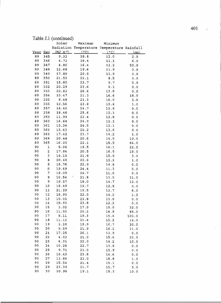
401
Year j2ay (MJ ________ (°o________ (mm)89 345 9 . 3 3 1 8 . 8 1 2 . 0 2 . 089 346 4 . 7 3 1 8 . 4 1 1 . 1 6 . 089 347 4 . 8 0 1 6 . 4 1 3 . 2 5 0 . 089 348 1 3 . 6 8 1 9 . 6 1 1 . 9 0 . 089 349 1 7 . 8 9 2 0 . 8 1 1 . 9 0 . 089 350 2 1 . 5 3 2 2 . 1 8 . 5 0 . 089 351 1 5 . 8 0 2 2 . 7 9 . 7 0 . 089 352 2 0 . 2 9 2 3 . 6 8 .3 0 . 089 353 2 0 . 8 3 2 6 . 6 1 3 . 8 0 . 089 354 1 0 . 4 7 2 1 . 3 1 6 . 6 1 8 . 089 355 8 . 4 8 2 1 . 3 1 6 . 0 5 . 089 356 1 2 . 5 6 2 3 . 8 1 3 . 4 1 . 089 357 1 4 . 4 6 2 4 . 7 1 2 . 9 0 . 089 358 1 8 . 4 6 2 5 . 6 1 2 .3 0 . 089 359 1 1 . 9 9 2 3 . 4 1 3 . 8 0 . 089 360 1 6 . 6 4 2 4 . 9 1 2 .3 0 . 089 361 1 5 . 3 4 2 4 . 5 1 2 . 1 0 . 089 362 1 5 .6 3 2 5 . 2 1 3 . 6 0 . 089 363 1 7 . 4 2 2 3 . 7 1 4 . 2 1 . 089 364 2 0 . 4 4 2 0 . 6 1 4 . 0 1 0 . 089 365 1 6 . 2 0 2 2 . 1 1 5 . 5 6 4 . 090 1 5 . 0 6 1 8 . 5 1 6 . 1 2 1 . 090 2 1 7 . 8 4 2 0 . 5 1 6 . 5 1 8 . 090 3 1 8 . 1 0 2 1 . 8 1 5 . 0 3 . 090 4 2 0 . 4 0 2 2 . 6 1 3 .3 1 . 090 5 1 8 . 7 6 2 2 . 9 1 4 . 8 0 . 090 .6 1 9 . 6 9 2 4 . 4 1 1 .3 0 . 090 7 1 8 . 0 9 2 4 . 7 1 1 . 0 0 . 090 8 1 0 . 5 4 ' 2 1 . 8 1 3 . 5 3 1 . 090 9 1 9 . 5 7 1 8 . 0 1 4 . 7 1 2 .090 10 1 8 . 4 9 1 9 . 7 1 2 . 8 0 . 090 11 2 1 . 2 9 1 9 . 5 1 3 . 7 6 . 090 ,12 1 8 . 9 5 2 2 . 0 1 4 . 2 1 . 090 13 1 5 . 0 1 2 3 . 8 1 3 . 0 0 . 090 14 1 5 .9 3 2 3 . 8 1 2 .3 0 . 090 15 3 . 0 2 1 7 . 0 1 5 . 0 3 2 . 090 16 1 1 . 5 0 2 0 . 2 1 4 . 9 4 5 . 090 17 8 . 1 1 1 9 . 3 1 5 .4 1 0 3 .090 18 1 1 . 1 2 2 1 . 4 1 5 .3 1 4 .090 19 3 . 3 8 1 9 . 9 1 6 . 7 3 0 . 090 20 5 . 5 9 2 1 . 9 1 6 . 1 1 1 .090 21 1 7 . 2 5 2 6 . 1 1 3 . 9 0 . 090 22 4 . 0 3 2 1 . 0 1 5 .4 2 3 . 090 23 6 . 9 1 2 2 . 0 1 4 . 2 1 0 .090 24 1 0 . 2 8 2 2 . 7 1 3 . 8 0 . 090 25 9 . 7 1 2 3 . 5 1 5 . 9 0 . 090 26 1 0 .4 3 2 3 . 8 1 6 . 6 0 . 090 27 1 3 . 8 8 2 3 . 0 1 6 . 8 1 . 090 28 1 5 .5 4 2 1 . 4 1 5 . 1 0 . 090 29 2 3 . 3 9 2 1 . 7 1 5 . 7 3 . 090 30 2 0 . 9 8 1 9 . 1 1 5 .3 1 0 .0
Table J.l (continued)S o l a r Maximum Minimum
R a d i a t i o n T e m p e r a tu r e T e m p e ra tu r e R a i n f a l l
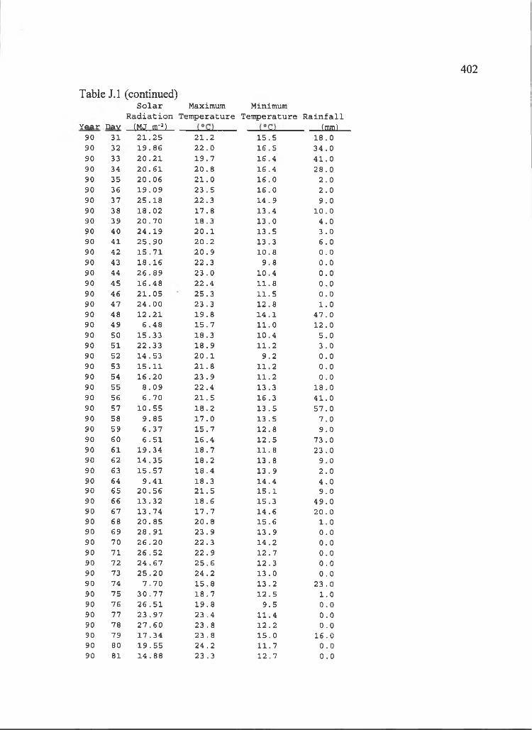
402
(MJ m- )____________________ (mm)2 1 . 2 5 2 1 . 21 9 . 8 6 2 2 . 02 0 . 2 1 1 9 . 72 0 . 6 1 2 0 . 82 0 . 0 6 2 1 . 01 9 . 0 9 2 3 . 52 5 . 1 8 2 2 . 31 8 . 0 2 1 7 . 82 0 . 7 0 1 8 .32 4 . 1 9 2 0 . 12 5 . 9 0 2 0 . 21 5 . 7 1 2 0 . 91 8 . 1 6 2 2 .32 6 . 8 9 2 3 . 01 6 . 4 8 2 2 . 42 1 . 0 5 2 5 .32 4 . 0 0 2 3 .31 2 . 2 1 1 9 . 8
6 . 4 8 1 5 . 71 5 .3 3 1 8 .32 2 . 3 3 1 8 . 91 4 .5 3 2 0 . 11 5 . 1 1 2 1 . 81 6 . 2 0 2 3 . 9
8 . 0 9 2 2 . 46 . 7 0 2 1 . 5
1 0 . 5 5 1 8 . 29 . 8 5 1 7 . 06 . 3 7 1 5 . 76 . 5 1 1 6 .4
1 9 . 3 4 1 8 . 71 4 . 3 5 1 8 .21 5 . 5 7 1 8 .4
9 . 4 1 18 .32 0 . 5 6 2 1 . 51 3 . 3 2 1 8 .61 3 . 7 4 1 7 . 72 0 . 8 5 2 0 . 82 8 . 9 1 2 3 . 92 6 . 2 0 2 2 . 32 6 . 5 2 2 2 . 92 4 . 6 7 2 5 . 62 5 . 2 0 2 4 . 2
7 . 7 0 1 5 .83 0 . 7 7 1 8 . 72 6 . 5 1 1 9 . 82 3 . 9 7 2 3 . 42 7 . 6 0 2 3 . 81 7 . 3 4 2 3 . 81 9 . 5 5 2 4 . 21 4 . 8 8 2 3 .3
Table J.l (continued)S o l a r Maximum Minimum
R a d i a t i o n T e m p e r a tu r e T e m p e ra tu r e R a i n f a l lYe ar Day
90 3190 3290 3390 3490 3590 3690 3790 3890 3990 4090 4190 4290 4390 4490 4590 4690 4790 4890 4990 5090 5190 5290 5390 5490 5590 5690 5790 5890 5990 6090 6190 6290 6390 6490 6590 6690 6790 6890 6990 7090 7190 7290 7390 7490 7590 7690 7790 7890 7990 8090 81
1 5 .5 1 8 . 01 6 .5 3 4 . 01 6 .4 4 1 . 01 6 .4 2 8 . 01 6 .0 2 . 01 6 .0 2 . 01 4 . 9 9 . 01 3 .4 1 0 . 01 3 .0 4 . 01 3 .5 3 . 01 3 .3 6 . 01 0 .8 0 . 0
9 .8 0 . 01 0 .4 0 . 01 1 .8 0 . 01 1 .5 0 . 01 2 . 8 1 . 01 4 . 1 4 7 . 01 1 .0 1 2 . 01 0 .4 5 . 01 1 .2 3 . 0
9 .2 0 . 01 1 .2 0 . 01 1 .2 0 . 01 3 .3 1 8 .01 6 .3 4 1 . 01 3 . 5 5 7 .01 3 . 5 7 . 01 2 .8 9 .01 2 . 5 73 .011. 8 2 3 . 01 3 .8 9 .01 3 . 9 2 . 014 .4 4 . 01 5 . 1 9 .01 5 .3 4 9 . 014 .6 2 0 . 01 5 . 6 1 . 01 3 . 9 0 . 01 4 . 2 0 . 01 2 . 7 0 . 012 . 3 0 . 013 .0 0 . 01 3 .2 23 .01 2 . 5 1 .0
9 .5 0 . 01 1 .4 0 . 01 2 .2 0 . 01 5 .0 1 6 .01 1 . 7 0 . 01 2 .7 0 . 0
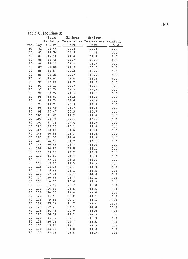
403
Table J.l (continued)S o l a r Maximum Minimum
R a d i a t i o n Temperature Temperature R a i n f a l l Y e a r E a z ( M J nr') L isn _______ (mm)
90 82 2 1 . 6 4 2 4 . 5 1 3 . 1 0 . 090 83 1 7 . 5 6 2 4 . 7 1 4 . 2 0 . 090 84 1 7 . 1 0 2 4 . 4 1 2 . 7 0 . 090 85 3 1 . 4 6 2 3 . 7 1 3 . 2 0 . 090 86 2 6 . 2 2 2 3 . 0 1 5 . 7 0 .090 87 2 9 . 8 0 2 4 . 0 1 3 . 6 5 . 090 88 3 1 . 6 7 2 0 . 2 1 3 . 9 4 . 090 89 2 8 . 2 5 2 0 . 7 1 3 . 9 1 . 090 90 2 8 . 0 1 2 1 . 0 1 3 . 8 4 . 090 91 2 8 . 2 0 2 1 . 7 1 4 . 2 0 . 090 92 2 2 . 1 0 2 2 . 7 1 2 . 7 0 . 090 93 '20 .74 2 1 . 2 1 2 . 7 2 . 090 94 2 0 . 7 2 2 1 . 5 1 2 . 1 1 . 090 95 1 5 . 8 0 2 3 . 2 1 1 . 8 0 . 090 96 2 3 . 7 4 2 5 . 6 1 1 . 5 0 . 090 97 1 4 .9 3 2 3 . 9 1 2 . 7 0 . 090 98 1 6 . 4 9 2 4 . 7 1 1 . 8 0 . 090 99 2 0 . 4 7 2 2 . 9 1 2 . 7 0 . 090 100 1 1 . 6 0 2 4 . 2 1 4 . 4 0 . 090 101 2 0 . 7 6 2 7 . 4 1 3 . 6 0 . 090 102 3 0 . 2 3 2 7 . 4 1 4 . 7 0 . 090 103 2 9 . 1 9 2 5 . 1 1 4 . 9 2 . 090 104 2 3 . 6 6 2 4 . 6 1 6 . 9 0 . 090 105 2 6 . 8 9 2 5 . 3 1 4 . 4 0 . 090 106 2 1 . 9 8 2 4 . 8 1 2 . 9 0 . 090 107 2 5 . 4 8 2 3 . 7 1 3 . 5 0 . 090 108 2 6 . 8 6 2 3 . 7 1 4 . 0 0 . 090 109 2 4 . 6 1 2 3 . 5 1 4 . 1 0 . 090 110 2 9 . 1 8 2 3 . 2 1 6 . 5 0 . 090 111 3 1 . 8 6 2 3 . 1 1 6 .3 3 . 090 112 2 9 . 1 1 2 3 . 2 1 5 .4 0 . 090 113 1 5 . 6 8 2 3 . 3 1 3 . 9 2 . 090 114 1 4 . 2 4 2 5 . 4 1 4 . 9 0 . 090 115 1 5 . 8 9 2 6 . 1 1 5 . 5 0 . 090 116 1 7 . 3 1 2 6 . 1 1 4 . 8 0 . 090 117 2 0 . 6 9 2 6 . 7 1 5 . 1 0 . 090 118 1 4 . 0 5 2 5 . 6 1 5 . 8 0 . 090 119 1 4 . 8 7 2 5 . 7 1 5 . 0 0 . 090 120 1 6 .9 3 2 4 . 5 1 4 . 6 0 . 090 121 2 4 . 7 0 2 3 . 8 1 4 . 6 0 . 090 122 2 4 . 4 8 2 5 . 2 1 3 . 1 0 . 090 123 9 . 8 3 2 1 . 3 1 4 . 1 3 2 . 090 124 2 5 . 5 4 2 1 . 7 1 3 . 4 1 4 .090 125 1 7 . 2 0 2 0 . 1 1 4 . 8 3 0 . 090 126 2 4 . 7 8 2 1 . 0 1 4 . 8 5 . 090 127 2 8 . 0 1 2 2 . 3 1 4 .3 2 . 090 128 2 4 . 7 8 2 1 . 4 1 5 .3 5 . 090 129 3 0 . 2 1 2 2 . 7 1 3 . 6 0 . 090 130 1 5 .8 6 2 3 . 1 1 3 . 9 2 . 090 131 2 3 . 5 0 2 4 . 0 1 4 .8 0 . 090 132 2 3 . 1 8 2 3 . 5 1 4 . 9 0 . 0

404
Y ea r Dav (MJ m~ )__________________ (°C)______(mm)90 133 2 5 . 1 0 2 3 . G 1 5 . 0 0 . 090 134 2 0 . 0 4 2 4 . 3 1 4 . 8 0 . 090 135 2 4 . 6 8 2 2 . 6 1 5 . 5 0 . 090 136 2 4 . 2 9 2 3 . 2 1 4 . 6 1 . 090 137 2 5 . 3 5 2 3 . 5 1 6 . 2 5 . 090 138 2 5 . 6 8 2 2 . 7 1 6 . 1 1 8 . 090 139 2 1 . 0 2 2 2 . 2 1 5 . 5 2 0 . 090 140 1 4 . 4 2 2 0 . 2 1 6 . 0 6 7 . 090 141 2 1 . 4 6 2 1 . 0 1 5 . 9 1 . 090 142 2 3 . 9 3 2 3 . 5 1 5 . 3 0 . 090 143 2 6 . 9 1 2 2 . 9 1 4 . 1 0 . 090 144 1 9 . 0 2 2 2 . 0 1 5 . 6 9 . 090 145 2 6 . 1 4 2 2 . 5 1 5 .3 1 .090 146 2 3 . 7 9 2 2 . 8 1 6 . 4 2 . 090 147 2 1 . 7 5 2 3 . 1 1 7 . 1 5 . 090 148 2 4 . 0 9 2 7 . 8 1 5 . 7 0 . 090 149 2 6 . 1 7 2 4 . 7 1 4 . 5 0 . 090 150 2 6 . 2 9 2 3 . 8 1 5 . 7 0 . 090 151 2 6 . 3 9 2 6 . 2 1 5 . 9 0 . 090 152 2 7 . 7 2 2 5 . 1 1 6 . 1 0 . 090 153 2 7 . 5 3 2 4 . 2 1 6 .3 0 . 090 154 2 5 . 3 4 2 5 . 1 1 6 . 1 1 . 090 155 2 5 . 6 2 2 5 . 3 1 7 . 1 0 . 090 156 1 9 . 6 1 2 4 . 4 1 7 . 2 2 . 090 157 1 9 .4 3 2 4 . 3 1 6 . 9 1 . 090 158 1 9 . 2 1 2 5 . 4 1 6 . 4 2 . 090 159 2 6 . 4 0 2 4 . 0 1 6 . 8 1 . 090 160 2 7 . 1 4 2 4 . 8 1 5 . 1 0 . 090 161 2 5 . 6 3 2 3 . 8 1 4 . 5 0 . 090 162 1 9 . 7 5 2 6 . 0 1 5 . 0 0 . 090 163 2 2 . 9 4 2 4 . 4 1 6 . 6 0 . 090 164 2 6 . 0 3 2 5 . 1 1 6 . 5 0 . 090 165 2 4 . 2 4 2 4 . 0 1 6 .8 1 1 . 090 166 1 6 . 7 4 2 2 . 0 1 6 . 8 2 7 . 090 167 1 5 . 4 5 2 0 . 2 1 6 . 7 5 6 . 090 168 1 9 . 2 3 2 1 . 4 1 6 . 0 1 1 . 090 169 2 0 . 6 2 2 1 . 2 1 6 . 0 2 4 . 090 170 2 2 . 2 6 2 3 . 4 1 5 . 9 1 3 . 090 171 1 5 .3 3 2 2 . 9 1 6 . 7 2 . 090 172 2 3 . 4 1 2 4 . 0 1 7 .3 0 . 090 173 2 4 . 4 9 2 2 . 5 1 6 . 5 1 .090 174 2 0 . 4 7 2 3 . 7 1 6 . 2 0 . 090 175 2 3 . 2 5 2 2 . 5 1 5 . 9 4 . 090 176 2 1 . 9 2 2 2 . 5 1 6 . 1 1 . 090 177 2 5 . 4 3 2 3 . 2 1 6 . 2 0 . 090 178 2 6 . 5 3 2 5 . 9 1 5 .4 0 . 090 179 2 6 . 4 1 2 4 . 2 1 7 . 5 0 . 090 180 2 3 . 3 9 2 3 . 8 1 7 . 5 2 . 090 181 2 1 . 3 8 2 4 . 4 1 7 .2 1 . 090 182 2 5 . 1 6 2 3 . 8 1 7 .4 1 . 090 183 2 4 . 9 2 2 4 . 0 1 7 . 5 3 . 0
Table J.l (continued)S o l a r Maximum Minimum
R a d i a t i o n T e m p e r a tu r e T e m p e r a tu r e R a i n f a l l
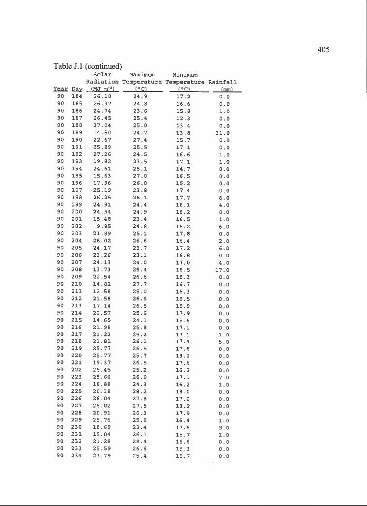
405
Xsa£ Cay (MJ nr l LlSLl _________ (mm)90 184 2 6 . 1 0 2 4 . 9 1 7 . 2 0 . 090 185 2 6 . 3 7 2 4 . 8 1 6 . 6 0 . 090 186 2 4 . 7 4 2 3 . 6 1 5 . 8 1 . 090 187 2 6 . 4 5 2 5 . 4 1 2 . 3 0 . 090 188 2 7 . 0 4 2 5 . 0 1 3 . 4 0 . 090 189 1 4 . 5 0 2 4 . 7 1 3 . 8 3 1 . 090 190 2 2 . 6 7 2 7 . 4 1 5 . 7 0 . 090 191 2 5 . 8 9 2 5 . 5 1 7 . 1 0 . 090 192 2 7 . 2 6 2 4 . 5 1 6 . 6 1 . 090 193 1 9 . 8 2 2 3 . 5 1 7 . 1 1 . 090 194 2 4 . 6 1 2 5 . 1 1 4 . 7 0 . 090 195 1 5 . 6 3 2 7 . 0 1 6 . 5 0 . 090 196 1 7 . 9 6 2 6 . 0 1 5 . 2 0 . 090 197 2 5 . 1 9 2 3 . 8 1 7 . 4 0 . 090 198 2 6 . 2 5 2 6 . 1 1 7 . 7 6 . 090 199 2 4 . 9 1 2 4 . 4 1 8 . 1 4 . 090 200 2 4 . 3 4 2 4 . 9 1 6 . 2 0 . 090 201 1 5 . 4 8 2 3 . 4 1 6 . 5 1 . 090 202 9 . 9 5 2 4 . 8 1 6 . 2 6 . 090 203 2 1 . 8 9 2 5 . 1 1 7 . 8 0 . 090 204 2 8 . 0 2 2 6 . 6 1 6 . 4 2 . 090 205 2 4 . 1 7 2 3 . 7 1 7 . 2 6 . 090 206 2 3 . 2 6 2 3 . 1 1 6 . 8 0 . 090 207 2 4 . 1 3 2 4 . 0 1 7 . 0 4 . 090 208 1 3 .7 3 2 5 . 4 1 8 . 5 1 7 .090 209 2 2 . 5 4 2 6 . 6 1 8 .3 0 . 090 210 1 4 . 8 2 2 7 . 7 1 6 . 7 0 . 090 211 1 2 . 5 8 2 5 . 0 1 6 .3 0 . 090 212 2 1 . 5 8 2 6 . 6 1 8 . 5 0 . 090 213 1 7 . 1 4 2 6 . 5 1 5 . 9 0 . 090 214 2 2 . 5 7 2 5 . 6 1 7 . 9 0 . 090 215 1 4 . 6 5 2 4 . 1 1 5 . 6 0 . 090 216 2 1 . 9 8 2 5 . 8 1 7 . 1 0 . 090 217 2 1 . 2 2 2 5 . 2 1 7 . 1 1 . 090 218 2 1 . 8 1 2 6 . 1 1 7 . 4 5 . 090 219 2 5 . 7 7 2 6 . 5 1 7 . 6 0 . 090 220 2 5 . 7 7 2 5 . 7 1 8 . 2 0 . 090 221 1 9 . 3 7 2 6 . 5 1 7 . 6 0 . 090 222 2 6 . 4 5 2 5 . 2 1 6 . 2 0 . 090 223 2 5 . 6 6 2 6 . 0 1 7 . 1 7 . 090 224 1 8 . 8 8 2 4 . 3 1 6 . 2 1 . 090 225 2 0 . 3 8 2 8 . 2 1 8 . 0 0 . 090 226 2 6 . 0 4 2 7 . 8 1 7 . 2 0 . 090 227 2 6 . 0 2 2 7 . 5 1 8 . 9 0 . 090 228 2 0 . 9 1 2 6 . 3 1 7 . 9 0 . 090 229 2 5 . 7 6 2 5 . 5 1 6 . 4 1 . 090 230 1 8 . 6 9 2 3 . 4 1 7 . 6 9 .090 231 1 5 .0 4 2 6 . 1 1 5 . 7 1 . 090 232 2 1 . 2 8 2 8 . 4 1 6 . 6 0 . 090 233 2 5 . 5 9 2 6 . 6 1 5 .3 0 .090 234 2 3 . 7 9 2 5 . 4 1 5 . 7 0 . 0
Table J.l (continued)S o l a r Maximum Minimum
R a d i a t i o n T e m p e r a tu r e T e m p e ra tu r e R a i n f a l l
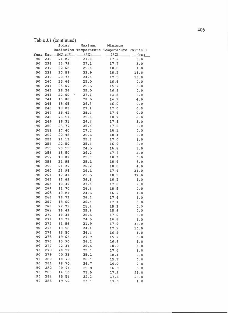
406
Y e a r Ca z (MJ __________________ m ______(mm)90 2 3 5 2 1 . 8 2 2 7 . 6 1 7 . 2 0 . 090 2 3 6 2 3 . 7 9 2 7 . 1 1 7 . 7 3 . 090 2 3 7 2 2 . 6 8 2 5 . 6 1 8 . 8 1 . 090 2 3 8 2 0 . 5 8 2 3 . 9 1 8 . 2 1 4 . 090 2 3 9 2 0 . 7 3 2 4 . 6 1 7 . 5 1 3 . 090 2 4 0 2 5 . 6 6 2 5 . 0 1 6 . 6 0 . 090 2 4 1 2 5 . 0 7 2 5 . 5 1 5 . 2 0 . 090 2 4 2 2 5 . 2 4 2 5 . 0 1 6 . 8 0 . 090 2 4 3 2 2 . 9 0 • 2 7 . 1 1 3 . 8 0 . 090 2 4 4 1 3 . 8 6 2 8 . 0 1 4 . 7 4 . 090 2 4 5 1 8 . 6 5 2 9 . 3 1 6 . 0 0 . 090 2 4 6 1 8 . 0 3 2 7 . 4 1 7 . 0 0 . 090 2 4 7 1 9 . 4 2 2 8 . 4 1 7 . 4 0 . 090 2 4 8 2 3 . 5 1 2 5 . 6 1 8 . 7 6 . 090 2 4 9 1 9 . 3 1 2 4 . 4 1 7 . 8 3 . 090 2 5 0 2 3 . 7 7 2 5 . 6 1 7 . 2 0 . 090 2 5 1 1 7 . 4 0 2 7 . 2 1 6 . 1 0 . 090 2 5 2 2 0 . 4 8 2 5 . 8 1 8 . 4 5 . 090 2 5 3 2 1 . 1 2 2 5 . 3 1 7 . 0 1 . 090 2 5 4 2 2 . 5 0 2 5 . 4 1 6 . 9 0 . 090 2 5 5 2 0 . 5 9 2 4 . 5 1 6 . 8 7 . 090 2 5 6 1 8 . 5 0 2 6 . 2 1 7 . 7 3 . 090 2 5 7 1 8 . 0 2 2 5 . 3 1 8 . 3 0 . 090 2 5 8 2 1 . 9 5 2 5 . 1 1 8 . 4 5 . 090 2 5 9 2 1 . 2 7 2 6 . 2 1 8 . 8 4 . 090 2 6 0 2 3 . 9 8 2 6 . 1 1 7 . 4 3 1 . 090 2 6 1 1 2 . 4 1 2 2 . 5 1 8 . 9 3 2 . 090 2 6 2 1 3 . 6 9 2 6 . 6 1 8 . 2 1 . 090 2 6 3 1 0 . 3 7 2 7 . 6 1 7 . 6 9 . 090 2 6 4 1 1 . 7 0 2 6 . 4 1 8 . 5 0 . 090 2 6 5 1 9 . 8 1 2 4 . 5 1 6 . 2 1 . 090 2 6 6 1 6 . 7 3 2 6 . 2 1 7 . 4 1 . 090 2 6 7 1 8 . 6 0 2 6 . 4 1 7 . 4 0 . 090 2 6 8 2 2 . 2 9 2 5 . 4 1 5 . 2 0 . 090 2 6 9 1 6 . 4 9 2 5 . 6 1 5 . 6 0 . 090 2 7 0 1 9 . 3 8 2 5 . 5 1 7 . 0 0 . 090 2 7 1 1 9 . 7 1 2 4 . 5 1 6 . 6 1 . 090 2 7 2 1 1 . 5 6 2 1 . 9 1 7 . 9 3 8 . 090 2 7 3 1 9 . 5 8 2 4 . 4 1 7 . 9 1 0 . 090 2 7 4 1 6 . 5 0 2 4 . 4 1 6 . 9 4 . 090 2 7 5 1 9 . 6 3 2 7 . 9 1 5 . 7 0 . 090 2 7 6 1 5 . 9 0 2 6 . 2 1 6 . 8 5 . 090 2 7 7 2 2 . 3 4 2 6 . 4 1 8 . 9 3 . 090 2 7 8 2 0 . 2 7 2 5 . 1 1 7 . 6 3 . 090 2 7 9 2 0 . 3 3 2 5 . 1 1 8 . 1 0 . 090 2 8 0 1 8 . 7 9 2 6 . 1 1 5 . 7 0 . 090 2 8 1 1 8 . 7 0 2 6 . 7 1 6 . 0 0 . 090 2 8 2 2 0 . 7 4 2 5 . 8 1 6 . 9 0 . 090 2 8 3 1 4 . 1 6 2 3 . 5 1 7 . 3 2 5 . 090 2 8 4 1 5 . 5 4 2 2 . 3 1 7 . 5 2 6 . 090 2 8 5 1 9 . 9 2 2 3 . 1 1 7 . 0 1 . 0
Table J .l (continued)S o l a r Maximum Minimum
R a d i a t i o n T e m p e r a tu r e T e m p e ra tu r e R a i n f a l l
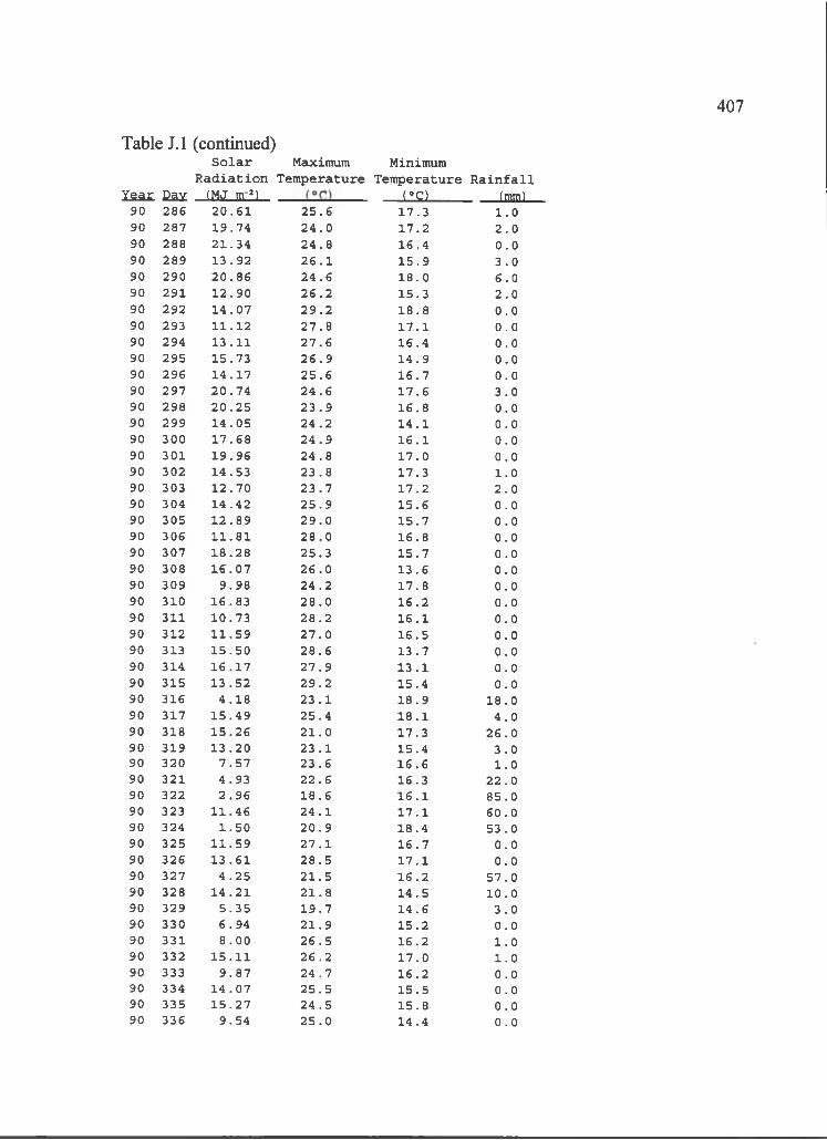
407
Y e a r C a y ( M J m '^ ) ______________________ ( ‘ O ______(mm)90 2 8 6 2 0 . 6 1 2 5 . 6 1 7 . 3 1 . 090 2 8 7 1 9 . 7 4 2 4 . 0 1 7 . 2 2 . 090 28 8 2 1 . 3 4 2 4 . 8 1 6 . 4 0 . 090 2 8 9 1 3 . 9 2 2 6 . 1 1 5 . 9 3 . 090 2 9 0 2 0 . 8 6 2 4 . 6 1 8 . 0 6 . 090 2 9 1 1 2 . 9 0 2 6 . 2 1 5 . 3 2 . 090 2 9 2 1 4 . 0 7 2 9 . 2 1 8 . 8 0 . 090 29 3 1 1 . 1 2 2 7 . 8 1 7 . 1 0 . 090 29 4 1 3 . 1 1 2 7 . 6 1 6 . 4 0 . 090 2 9 5 1 5 . 7 3 2 6 . 9 1 4 . 9 0 . 090 2 9 6 1 4 . 1 7 2 5 . 6 1 6 . 7 0 . 090 2 9 7 2 0 . 7 4 2 4 . 6 1 7 . 6 3 . 090 2 9 8 2 0 . 2 5 2 3 . 9 1 6 . 8 0 . 090 2 9 9 1 4 . 0 5 2 4 . 2 1 4 . 1 0 . 090 3 0 0 1 7 . 6 8 2 4 . 9 1 6 . 1 0 . 090 3 0 1 1 9 . 9 6 2 4 . 8 1 7 . 0 0 . 090 3 0 2 1 4 . 5 3 2 3 . 8 1 7 . 3 1 . 090 30 3 1 2 . 7 0 2 3 . 7 1 7 . 2 2 . 090 3 0 4 1 4 . 4 2 2 5 . 9 1 5 . 6 0 . 090 3 0 5 1 2 . 8 9 2 9 . 0 1 5 . 7 0 . 090 3 0 6 1 1 . 8 1 2 8 . 0 1 6 . 8 0 . 090 3 0 7 1 8 . 2 8 2 5 . 3 1 5 . 7 0 . 090 3 0 8 1 6 . 0 7 2 6 . 0 1 3 . 6 0 . 090 3 0 9 9 . 9 8 2 4 . 2 1 7 . 8 0 . 090 3 1 0 1 6 . 8 3 2 8 . 0 1 6 . 2 0 . 090 3 1 1 1 0 . 7 3 2 8 . 2 1 6 . 1 0 . 090 3 1 2 1 1 . 5 9 2 7 . 0 1 6 . 5 0 . 090 3 1 3 1 5 . 5 0 2 8 . 6 1 3 . 7 0 . 090 3 1 4 1 6 . 1 7 2 7 . 9 1 3 . 1 0 . 090 3 1 5 1 3 . 5 2 2 9 . 2 1 5 . 4 0 . 090 3 1 6 4 . 1 8 2 3 . 1 1 8 . 9 1 8 . 090 3 1 7 1 5 . 4 9 2 5 . 4 1 8 . 1 4 . 090 3 1 8 1 5 . 2 6 2 1 . 0 1 7 . 3 2 6 . 090 3 1 9 1 3 . 2 0 2 3 . 1 1 5 . 4 3 . 090 3 2 0 7 . 5 7 2 3 . 6 1 6 . 6 1 . 090 3 2 1 4 . 9 3 2 2 . 6 1 6 . 3 2 2 . 090 3 2 2 2 . 9 6 1 8 . 6 1 6 . 1 8 5 . 090 3 2 3 1 1 . 4 6 2 4 . 1 1 7 . 1 6 0 . 090 3 2 4 1 . 5 0 2 0 . 9 1 8 . 4 5 3 . 090 3 2 5 1 1 . 5 9 2 7 . 1 1 6 . 7 0 . 090 3 2 6 1 3 . 6 1 2 8 . 5 1 7 . 1 0 . 090 3 2 7 4 . 2 5 2 1 . 5 1 6 . 2 5 7 . 090 3 2 8 1 4 . 2 1 2 1 . 8 1 4 . 5 1 0 . 090 3 2 9 5 . 3 5 1 9 . 7 1 4 . 6 3 . 090 3 3 0 6 . 9 4 2 1 . 9 1 5 . 2 0 . 090 3 3 1 8 . 0 0 2 6 . 5 1 6 . 2 1 . 090 3 3 2 1 5 . 1 1 2 6 . 2 1 7 . 0 1 . 090 3 3 3 9 . 8 7 2 4 . 7 1 6 . 2 0 . 090 3 3 4 1 4 . 0 7 2 5 . 5 1 5 . 5 0 . 090 3 3 5 1 5 . 2 7 2 4 . 5 1 5 . 8 0 . 090 3 3 6 9 . 5 4 2 5 . 0 1 4 . 4 0 . 0
Table J .l (continued)S o l a r Maximum Minimum
R a d i a t i o n T e m p e r a tu r e T e m p e r a tu r e R a i n f a l l
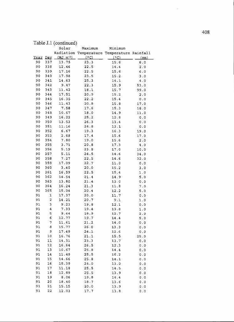
408
Y e a r C a y (MJ _____ ( » c ) ( ° o ______________(mm)90 3 3 7 1 3 . 7 5 2 3 . 3 1 5 . 6 6 . 090 3 3 8 1 2 . 4 6 2 2 . 5 1 4 . 4 2 . 090 3 3 9 1 7 . 1 6 2 2 . 5 1 5 . 6 6 . 090 3 4 0 1 7 . 9 8 2 3 . 5 1 5 . 2 3 . 090 3 4 1 1 4 . 6 3 2 5 . 3 1 4 . 1 4 . 090 3 4 2 9 . 4 7 2 2 . 3 1 5 . 9 5 3 . 090 3 4 3 1 1 . 4 2 1 8 . 1 1 5 . 7 9 9 . 090 3 4 4 1 7 . 5 1 2 0 . 9 1 5 . 2 2 . 090 3 4 5 1 6 . 3 5 2 2 . 2 1 5 . 4 0 . 090 3 4 6 1 1 . 4 3 2 0 . 8 1 5 . 8 1 7 . 090 3 4 7 7 . 5 8 1 7 . 6 1 5 . 3 1 8 . 090 3 4 8 1 0 . 6 7 1 8 . 0 1 4 . 9 1 1 . 090 3 4 9 1 6 . 2 2 2 5 . 2 1 2 . 8 0 . 090 3 5 0 1 3 . 5 3 2 6 . 3 1 3 . 4 0 . 090 3 5 1 1 1 . 1 6 2 4 . 8 1 3 . 1 0 . 090 3 5 2 6 . 6 7 1 9 . 3 1 6 . 3 1 9 . 090 3 5 3 2 . 6 8 1 7 . 4 1 5 . 6 1 7 . 090 3 5 4 7 . 8 0 1 9 . 0 1 5 . 6 2 . 090 3 5 5 3 . 7 1 2 0 . 8 1 7 . 3 4 . 090 3 5 6 5 . 1 9 2 3 . 8 1 7 . 0 1 0 . 090 3 5 7 5 . 1 1 2 4 . 5 1 4 . 6 3 4 . 090 3 5 8 7 . 2 7 2 2 . 5 1 4 . 6 3 2 . 090 3 5 9 1 7 . 0 9 2 2 . 7 1 1 . 0 0 . 090 3 6 0 3 . 4 0 2 0 . 0 1 5 . 2 3 . 090 3 6 1 1 6 . 5 9 2 2 . 5 1 5 . 4 1 . 090 3 6 2 1 4 . 5 4 2 1 . 4 1 4 . 9 5 . 090 36 3 1 3 . 8 0 2 1 . 4 1 3 . 0 0 . 090 3 6 4 1 6 . 2 4 2 1 . 3 1 1 . 8 7 . 090 3 6 5 1 5 . 0 4 2 0 . 4 1 2 . 2 5 . 091 1 1 7 . 3 7 2 0 . 0 1 1 . 7 0 . 091 2 1 4 . 2 1 2 0 . 7 9 . 1 1 . 09 1 3 9 . 2 3 1 9 . 8 1 2 . 1 0 . 09 1 4 7 . 3 3 1 9 . 4 1 3 . 8 1 . 091 5 9 . 4 4 1 8 . 9 1 2 . 7 2 . 091 6 1 2 . 7 7 1 9 . 7 1 4 . 4 5 . 09 1 7 1 1 . 6 1 2 1 . 2 1 4 . 0 0 . 091 8 1 5 . 7 7 2 6 . 0 1 3 . 3 0 . 091 9 1 7 . 4 9 2 4 . 1 1 2 . 6 0 . 091 10 1 6 . 7 6 2 1 . 1 1 5 . 5 2 5 . 091 11 1 4 . 3 1 2 3 . 3 1 3 . 7 0 . 091 12 1 6 . 6 4 2 6 . 5 1 2 . 3 0 . 09 1 13 1 0 . 6 7 2 5 . 8 1 4 . 4 0 . 091 14 1 1 . 4 9 2 5 . 5 1 6 . 2 0 . 091 15 1 4 . 6 6 2 5 . 8 1 4 . 1 0 . 091 16 1 5 . 3 9 2 4 . 0 1 3 . 0 0 . 091 17 1 1 . 1 8 2 5 . 5 1 4 . 5 0 . 091 18 1 2 . 8 9 2 5 . 5 1 3 . 9 0 . 091 19 8 . 0 6 1 9 . 8 1 4 . 4 0 . 091 2 0 1 8 . 4 0 1 8 . 7 1 3 . 6 0 . 091 21 1 5 . 1 5 2 0 . 0 1 3 . 9 0 . 091 22 1 2 . 0 3 1 7 . 7 1 3 . 8 0 . 0
Table J .l (continued)S o l a r Maximum Minimum
R a d i a t i o n T e m p e r a tu r e T e m p e ra tu r e R a i n f a l l
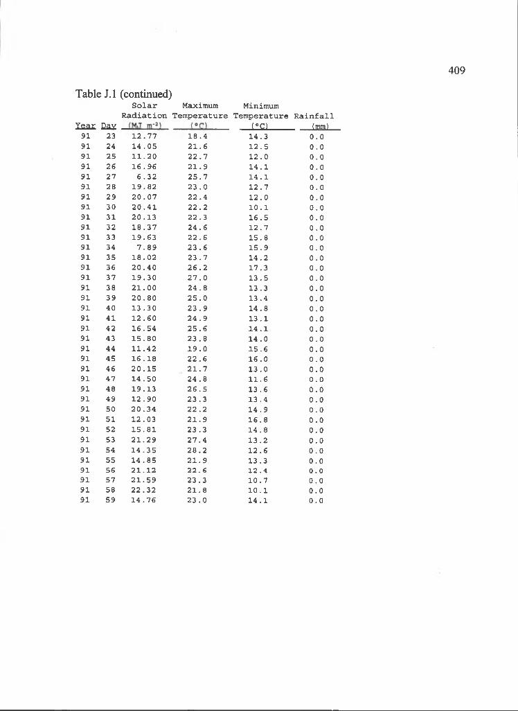
409
Y e a r C a y ( ° o _(mm)91 23 1 2 . 7 7 1 8 . 4 1 4 . 3 0 . 091 24 1 4 . 0 5 2 1 . 6 1 2 . 5 0 . 091 25 1 1 . 2 0 2 2 . 7 1 2 . 0 0 . 091 26 1 6 . 9 6 2 1 . 9 1 4 . 1 0 . 091 2 7 6 . 3 2 2 5 . 7 1 4 . 1 0 . 091 28 1 9 . 8 2 2 3 . 0 1 2 . 7 0 . 091 2 9 2 0 . 0 7 2 2 . 4 1 2 . 0 0 . 091 30 2 0 . 4 1 2 2 . 2 1 0 . 1 0 . 091 31 2 0 . 1 3 2 2 . 3 1 6 . 5 0 . 091 32 1 8 . 3 7 2 4 . 6 1 2 . 7 0 . 091 33 1 9 . 6 3 2 2 . 6 1 5 . 8 0 . 091 34 7 . 8 9 2 3 . 6 1 5 . 9 0 . 091 35 1 8 . 0 2 2 3 . 7 1 4 . 2 0 . 091 36 2 0 . 4 0 2 6 . 2 1 7 . 3 0 . 091 37 1 9 . 3 0 2 7 . 0 1 3 . 5 0 . 091 38 2 1 . 0 0 2 4 . 8 1 3 . 3 0 . 091 39 2 0 . 8 0 2 5 . 0 1 3 . 4 0 . 091 40 1 3 . 3 0 2 3 . 9 1 4 . 8 0 . 091 41 1 2 . 6 0 2 4 . 9 1 3 . 1 0 . 091 4 2 1 6 . 5 4 2 5 . 6 1 4 . 1 0 . 091 43 1 5 . 8 0 2 3 . 8 1 4 . 0 0 . 091 44 1 1 . 4 2 1 9 . 0 1 5 . 6 0 . 09 1 4 5 1 6 . 1 8 2 2 . 6 1 6 . 0 0 . 091 46 2 0 . 1 5 2 1 . 7 1 3 . 0 0 . 091 4 7 1 4 . 5 0 2 4 . 8 1 1 . 6 0 . 091 48 1 9 . 1 3 2 6 . 5 1 3 . 6 0 . 091 4 9 1 2 . 9 0 2 3 . 3 1 3 . 4 0 . 091 50 2 0 . 3 4 2 2 . 2 1 4 . 9 0 . 091 5 1 1 2 . 0 3 2 1 . 9 1 6 . 8 0 . 09 1 52 1 5 . 8 1 2 3 . 3 1 4 . 8 0 . 091 53 2 1 . 2 9 2 7 . 4 1 3 . 2 0 . 091 54 1 4 . 3 5 2 8 . 2 1 2 . 6 0 . 091 55 1 4 . 8 5 2 1 . 9 1 3 . 3 0 . 091 56 2 1 . 1 2 2 2 . 6 1 2 . 4 0 . 091 57 2 1 . 5 9 2 3 . 3 1 0 . 7 0 . 091 58 2 2 . 3 2 2 1 . 8 1 0 . 1 0 . 091 59 1 4 . 7 6 2 3 . 0 1 4 . 1 0 . 0
Table J .l (continued)S o l a r Maximum Minimum
R a d i a t i o n T e m p e r a tu r e T e m p e ra tu r e R a i n f a l l
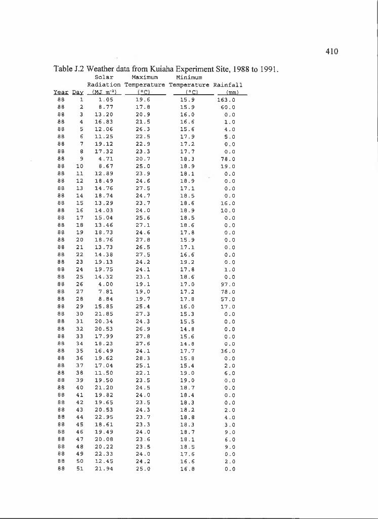
410
Table J.2 Weather data from Kuiaha Experiment Site, 1988 to 1991.S o l a r Maximum Minimum
R a d i a t i o n Temperatur e Temperature R a i n f a l l Year Cay . (MJ. nr ' ) ______ LliiLl__________ (mm)
88 1 1 . 0 5 1 9 . 688 2 8 . 7 7 1 7 . 888 3 1 3 . 2 0 2 0 . 988 4 1 6 . 8 3 2 1 . 588 5 1 2 . 0 6 2 6 . 388 6 1 1 . 2 5 2 2 . 588 7 1 9 . 1 2 2 2 . 988 8 1 7 . 3 2 2 3 . 388 9 4 . 7 1 2 0 . 788 10 8 . 6 7 2 5 . 088 11 1 2 . 8 9 2 3 . 988 12 1 8 . 4 9 2 4 . 688 13 1 4 . 7 6 2 7 . 588 14 1 8 . 7 4 2 4 . 788 15 1 3 . 2 9 2 3 . 788 16 1 4 . 0 3 2 4 . 088 17 1 5 . 0 4 2 5 . 688 18 1 3 . 4 6 2 7 . 188 19 1 8 . 7 3 2 4 . 688 20 1 8 . 7 6 2 7 . 888 2 1 1 3 . 7 3 2 6 . 588 22 1 4 . 3 8 2 7 . 588 23 1 9 . 1 3 2 4 . 288 24 1 9 . 7 5 2 4 . 188 25 1 4 . 3 2 2 3 . 188 26 4 . 0 0 1 9 . 188 2 7 7 . 8 1 1 9 . 088 28 8 . 8 4 1 9 . 788 2 9 1 5 . 8 5 2 5 . 488 30 2 1 . 8 5 2 7 . 388 31 2 0 . 3 4 2 4 . 388 32 2 0 . 5 3 2 6 . 988 33 1 7 . 9 9 2 7 . 888 34 1 8 . 2 3 2 7 . 688 3 5 1 6 . 4 9 2 4 . 188 36 1 9 . 6 2 2 8 . 388 3 7 1 7 . 0 4 2 5 . 188 38 1 1 . 5 0 2 2 . 188 39 1 9 . 5 0 2 3 . 588 40 2 1 . 2 0 2 4 . 588 4 1 1 9 . 8 2 2 4 . 088 42 1 9 . 6 5 2 3 . 588 43 2 0 . 5 3 2 4 . 388 44 2 2 . 9 5 2 3 . 788 4 5 1 8 . 6 1 2 3 . 388 4 6 1 9 . 4 9 2 4 . 088 4 7 2 0 . 0 8 2 3 . 688 48 2 0 . 2 2 2 3 . 588 4 9 2 2 . 3 3 2 4 . 088 50 1 2 . 4 5 2 4 . 288 51 2 1 . 9 4 2 5 . 0
1 5 . 9 1 6 3 . 01 5 . 9 6 0 . 01 6 . 0 0 . 01 6 . 6 1 . 01 5 . 6 4 . 01 7 . 9 5 . 01 7 . 2 0 . 01 7 . 7 0 . 01 8 . 3 7 8 . 01 8 . 9 1 9 . 01 8 . 1 0 . 01 8 . 9 0 . 01 7 . 1 0 . 01 8 . 5 0 . 01 8 . 6 1 6 . 01 8 . 9 10 . 01 8 . 5 0 . 018 . 6 0 . 01 7 . 8 0 . 01 5 . 9 0 . 01 7 . 1 0 . 01 6 . 6 0 . 01 9 . 2 0 . 01 7 . 8 1 . 01 8 . 6 0 . 01 7 . 0 9 7 . 01 7 . 2 7 8 . 01 7 . 8 5 7 . 01 6 . 0 1 7 . 01 5 . 3 0 . 01 5 . 5 0 . 014 . 8 0 . 01 5 . 6 0 . 014 . 6 0 . 01 7 . 7 3 6 . 01 5 . 8 0 . 01 5 . 4 2 . 01 9 . 0 6 . 01 9 . 0 0 . 018 . 7 0 . 018 . 4 0 . 018 . 3 0 . 01 8 . 2 2 . 01 8 . 8 4 . 01 8 . 3 3 . 01 8 . 7 9 . 01 8 . 1 6 . 01 8 . 5 9 . 01 7 . 6 0 . 016 . 6 2 . 01 6 . 8 0 . 0
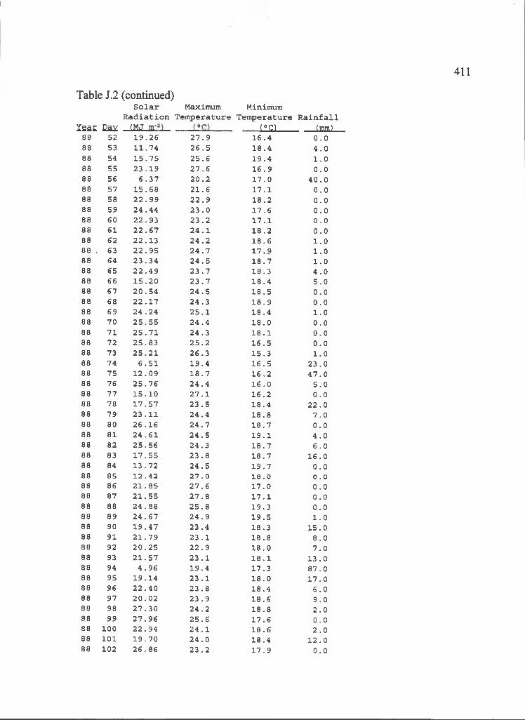
411
Table J.2 (continued)S o l a r Maximum Minimum
R a d i a t i o n Tem peratur e Temperature R a i n f a l l Year Cay (MJ _____________ (°o ____(mm)
88 52 1 9 . 2 6 2 7 . 988 53 1 1 . 7 4 2 6 . 588 54 1 5 . 7 5 2 5 . 688 55 2 3 . 1 9 2 7 . 688 56 6 . 3 7 2 0 . 288 57 1 5 . 6 8 2 1 . 688 58 2 2 . 9 9 2 2 . 988 59 2 4 . 4 4 2 3 . 088 60 2 2 . 9 3 2 3 . 288 61 2 2 . 6 7 2 4 . 188 62 2 2 . 1 3 2 4 . 288 . 6 3 2 2 . 9 5 2 4 . 788 64 2 3 . 3 4 2 4 . 588 6 5 2 2 . 4 9 2 3 . 788 6 6 1 5 . 2 0 2 3 . 788 6 7 2 0 . 5 4 2 4 . 588 68 2 2 . 1 7 2 4 . 388 6 9 2 4 . 2 4 2 5 . 188 70 2 5 . 5 5 2 4 . 488 71 2 5 . 7 1 2 4 . 388 72 2 5 . 8 3 2 5 . 288 73 2 5 . 2 1 2 6 . 388 74 6 . 5 1 1 9 . 488 75 1 2 . 0 9 1 8 . 788 76 2 5 . 7 6 2 4 . 488 77 1 5 . 1 0 2 7 . 188 78 1 7 . 5 7 2 3 . 588 79 2 3 . 1 1 2 4 . 488 80 2 6 . 1 6 2 4 . 788 81 2 4 . 6 1 2 4 . 588 82 2 5 . 5 6 2 4 . 388 83 1 7 . 5 5 2 3 . 888 84 1 3 . 7 2 2 4 . 588 85 1 2 . 4 2 2 7 . 088 86 2 1 . 8 5 2 7 . 688 87 2 1 . 5 5 2 7 . 888 88 2 4 . 8 8 2 5 . 888 89 2 4 . 6 7 2 4 . 988 90 1 9 . 4 7 2 3 . 488 91 2 1 . 7 9 2 3 . 188 92 2 0 . 2 5 2 2 . 988 93 2 1 . 5 7 2 3 . 188 94 4 . 9 6 1 9 . 488 95 1 9 . 1 4 2 3 . 188 96 2 2 . 4 0 2 3 . 888 97 2 0 . 0 2 2 3 . 988 98 2 7 . 3 0 2 4 . 288 99 2 7 . 9 6 2 5 . 688 10 0 2 2 . 9 4 2 4 . 188 1 0 1 1 9 . 7 0 2 4 . 088 10 2 2 6 . 8 6 2 3 . 2
1 6 . 4 0 . 01 8 . 4 4 . 01 9 . 4 1 . 01 6 . 9 0 . 01 7 . 0 4 0 . 01 7 . 1 0 . 01 8 . 2 0 . 01 7 . 6 0 . 01 7 . 1 0 . 01 8 . 2 0 . 01 8 . 6 1 . 01 7 . 9 1 . 01 8 . 7 1 . 01 8 . 3 4 . 01 8 . 4 5 . 01 8 . 5 0 . 01 8 . 9 0 . 01 8 . 4 1 . 01 8 . 0 0 . 01 8 . 1 0 . 01 6 . 5 0 . 01 5 . 3 1 . 01 6 . 5 2 3 . 016 . 2 4 7 . 01 6 . 0 5 . 01 6 . 2 0 . 01 8 . 4 22 . 01 8 . 8 7 . 01 8 . 7 0 . 01 9 . 1 4 . 01 8 . 7 6 . 01 8 . 7 1 6 . 01 9 . 7 0 . 018 . 0 0 . 01 7 . 0 0 . 01 7 . 1 0 . 01 9 . 3 0 . 01 9 . 5 1 . 01 8 . 3 1 5 . 01 8 . 8 8 . 01 8 . 0 7 . 01 8 . 1 13 . 01 7 . 3 8 7 . 01 8 . 0 1 7 . 01 8 . 4 6 . 018 . 6 9 . 01 8 . 8 2 . 01 7 . 6 0 . 018 . 6 2 . 018 . 4 1 2 . 01 7 . 9 0 . 0
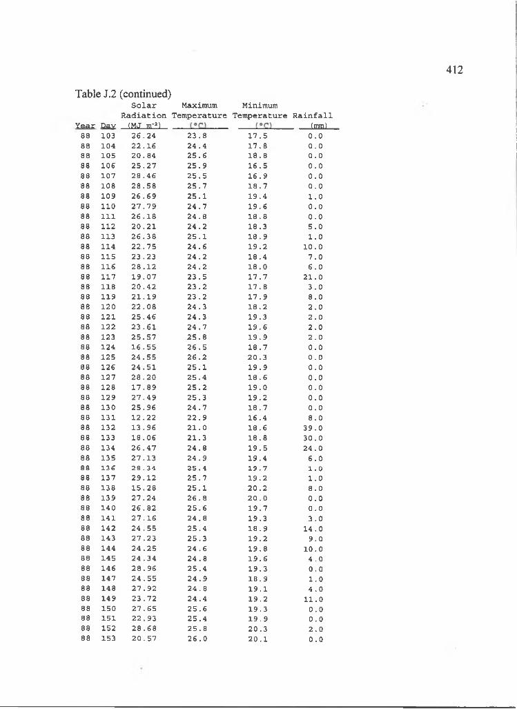
412
Table J.2 (continued)S o l a r Maximum Minimum
R a d i a t i o n Tem peratur e Temperature R a i n f a l lY ea r Dav (MJ m' )______________________________ (mm)
88 1 03 2 6 . 2 4 2 3 . 8 1 7 . 5 0 . 088 1 0 4 2 2 . 1 6 2 4 . 4 1 7 . 8 0 . 088 1 0 5 2 0 . 8 4 2 5 . 6 1 8 . 8 0 . 088 10 6 2 5 . 2 7 2 5 . 9 1 6 . 5 0 . 088 1 0 7 2 8 . 4 6 2 5 . 5 1 6 . 9 0 . 088 10 8 2 8 . 5 8 2 5 . 7 1 8 . 7 0 . 088 10 9 2 6 . 6 9 2 5 . 1 1 9 . 4 1 . 088 11 0 2 7 . 7 9 2 4 . 7 1 9 . 6 0 . 088 1 1 1 2 6 . 1 8 2 4 . 8 1 8 . 8 0 . 088 11 2 2 0 . 2 1 2 4 . 2 1 8 . 3 5 . 088 113 2 6 . 3 8 2 5 . 1 1 8 . 9 1 . 088 11 4 2 2 . 7 5 2 4 . 6 1 9 . 2 1 0 . 088 1 1 5 2 3 . 2 3 2 4 . 2 1 8 . 4 7 . 088 1 1 6 2 8 . 1 2 2 4 . 2 1 8 . 0 6 . 088 1 1 7 1 9 . 0 7 2 3 . 5 1 7 . 7 2 1 . 088 1 1 8 2 0 . 4 2 2 3 . 2 1 7 . 8 3 . 088 1 1 9 2 1 . 1 9 2 3 . 2 1 7 . 9 8 . 088 1 2 0 2 2 . 0 8 2 4 . 3 1 8 . 2 2 . 088 1 2 1 2 5 . 4 6 2 4 . 3 1 9 . 3 2 . 088 12 2 2 3 . 6 1 2 4 . 7 1 9 . 6 2 . 088 123 2 5 . 5 7 2 5 . 8 1 9 . 9 2 . 088 12 4 1 6 . 5 5 2 6 . 5 1 8 . 7 0 . 088 1 2 5 2 4 . 5 5 2 6 . 2 2 0 . 3 0 . 088 1 2 6 2 4 . 5 1 2 5 . 1 1 9 . 9 0 . 088 1 2 7 2 8 . 2 0 2 5 . 4 1 8 . 6 0 . 088 12 8 1 7 . 8 9 2 5 . 2 1 9 . 0 0 . 088 1 2 9 2 7 . 4 9 2 5 . 3 1 9 . 2 0 . 088 1 3 0 2 5 . 9 6 2 4 . 7 1 8 . 7 0 . 088 1 3 1 1 2 . 2 2 2 2 . 9 1 6 . 4 8 . 088 13 2 1 3 . 9 6 2 1 . 0 1 8 . 6 3 9 . 088 133 1 8 . 0 6 2 1 . 3 1 8 . 8 3 0 . 088 13 4 2 6 . 4 7 2 4 . 8 1 9 . 5 2 4 . 088 1 3 5 2 7 . 1 3 2 4 . 9 1 9 . 4 6 . 008 1 3 6 2 8 . 3 4 2 5 . 4 1 9 . 7 1 . 088 1 3 7 2 9 . 1 2 2 5 . 7 1 9 . 2 1 . 088 13 8 1 5 . 2 8 2 5 . 1 2 0 . 2 8 . 088 1 3 9 2 7 . 2 4 2 6 . 8 2 0 . 0 0 . 088 1 4 0 2 6 . 8 2 2 5 . 6 1 9 . 7 0 . 088 1 4 1 2 7 . 1 6 2 4 . 8 1 9 . 3 3 . 088 1 4 2 2 4 . 5 5 2 5 . 4 1 8 . 9 1 4 . 088 143 2 7 . 2 3 2 5 . 3 1 9 . 2 9 . 088 1 4 4 2 4 . 2 5 2 4 . 6 1 9 . 8 1 0 . 088 1 4 5 2 4 . 3 4 2 4 . 8 1 9 . 6 4 . 088 1 4 6 2 8 . 9 6 2 5 . 4 1 9 . 3 0 . 088 1 4 7 2 4 . 5 5 2 4 . 9 1 8 . 9 1 . 088 14 8 2 7 . 9 2 2 4 . 8 1 9 . 1 4 . 088 1 4 9 2 3 . 7 2 2 4 . 4 1 9 . 2 1 1 . 088 1 5 0 2 7 . 6 5 2 5 . 6 1 9 . 3 0 . 088 1 5 1 2 2 . 9 3 2 5 . 4 1 9 . 9 0 . 088 15 2 2 8 . 6 8 2 5 . 8 2 0 . 3 2 . 088 15 3 2 0 . 5 7 2 6 . 0 2 0 . 1 0 . 0

413
Table J.2 (continued)S o l a r Maximum Minimum
R a d i a t i o n Tem perat ure Temperature R a i n f a l lY e a r Cay (MJ ________LIO______ (mm)
88 1 54 2 0 . 8 0 2 5 . 7 2 0 . 4 3 . 088 1 5 5 2 2 . 9 6 2 5 . 2 2 0 . 1 1 . 088 15 6 2 5 . 5 3 2 5 . 0 1 9 . 7 2 . 088 1 5 7 2 9 . 5 7 2 6 . 1 2 0 . 0 4 . 088 15 8 2 8 . 2 7 2 5 . 2 1 9 . 4 0 . 088 1 5 9 2 1 . 8 4 2 5 . 3 1 9 . 9 1 1 . 088 1 6 0 2 7 . 4 1 2 4 . 9 1 9 . 3 1 0 . 088 1 6 1 2 8 . 7 0 2 5 . 5 1 9 . 5 3 . 088 1 6 2 2 8 . 5 9 2 6 . 1 1 9 . 7 1 . 0 -88 163 2 8 . 5 2 2 6 . 1 1 9 . 3 0 . 088 164 2 6 . 0 4 2 6 . 2 1 9 . 8 0 . 088 1 6 5 2 8 . 8 3 2 6 . 3 1 9 . 9 0 . 088 1 6 6 2 2 . 9 8 2 5 . 5 2 0 . 0 1 . 088 1 6 7 2 9 . 9 4 2 6 . 0 1 9 . 7 0 . 088 16 8 2 6 . 7 3 2 6 . 0 1 9 . 4 0 . 088 1 6 9 2 6 . 5 2 2 6 . 5 1 9 . 7 0 . 088 17 0 2 9 . 5 9 2 6 . 5 2 0 . 1 0 . 088 1 7 1 2 9 . 1 5 2 5 . 9 1 9 . 8 1 . 088 17 2 2 1 . 1 1 2 4 . 8 1 9 . 7 4 . 088 173 2 4 . 7 4 2 6 . 0 1 9 . 9 1 . 088 17 4 2 5 . 5 3 2 6 . 8 2 0 . 8 4 . 088 1 7 5 2 7 . 3 1 2 5 . 6 2 0 . 2 5 . 088 1 7 6 2 7 . 4 5 2 5 . 9 1 9 . 3 3 . 088 1 7 7 2 8 . 3 6 2 6 . 3 2 0 . 0 3 . 088 1 7 8 2 5 . 1 3 2 5 . 6 2 0 . 3 4 . 088 1 7 9 2 7 . 7 5 2 6 . 0 2 0 . 6 1 . 088 1 8 0 2 9 . 8 7 2 6 . 0 2 0 . 3 3 . 088 1 8 1 2 5 . 6 7 2 6 . 5 2 0 . 5 1 . 088 1 8 2 2 9 . 1 8 2 7 . 1 2 0 . 3 0 . 088 183 2 8 . 4 9 2 7 . 0 2 0 . 3 0 . 088 1 8 4 2 5 . 2 9 2 5 . 2 1 9 . 8 0 . 088 1 8 5 2 8 . 3 0 2 6 . 1 2 0 . 4 0 . 088 1 8 6 2 8 . 1 3 2 6 . 5 2 0 . 1 4 . 088 1 8 7 2 8 . 5 8 2 6 . 1 2 0 . 3 3 . 088 1 8 8 2 7 . 0 4 2 5 . 4 2 0 . 3 2 1 . 088 1 8 9 2 8 . 0 6 2 6 . 1 2 0 . 1 1 1 . 088 1 9 0 2 3 . 2 6 2 5 . 6 2 0 . 3 6 . 088 1 9 1 2 4 . 5 9 2 5 . 0 2 0 . 1 4 . 088 1 9 2 2 8 . 5 0 2 5 . 8 1 9 . 7 5 . 088 1 93 2 1 . 5 9 2 5 . 7 2 0 . 5 5 . 088 1 94 2 1 . 6 0 2 7 . 2 1 9 . 6 9 . 088 1 9 5 2 8 . 8 8 2 6 . 4 2 0 . 5 1 . 088 1 9 6 2 7 . 9 7 2 5 . 7 2 0 . 2 1 . 088 1 9 7 2 7 . 1 7 2 5 . 8 2 0 . 3 2 . 088 1 9 8 2 6 . 2 8 2 6 . 3 2 0 . 3 0 . 088 1 9 9 2 6 . 7 2 2 6 . 4 2 0 . 7 1 . 088 2 0 0 2 2 . 0 6 2 5 . 5 2 0 . 7 2 . 088 2 0 1 2 7 . 7 4 2 6 . 3 2 0 . 3 1 . 088 2 0 2 2 7 . 5 3 2 5 . 6 2 0 . 0 0 . 088 2 0 3 2 6 . 0 6 2 6 . 9 1 9 . 5 2 1 . 088 2 0 4 2 8 . 0 6 2 6 . 5 2 0 . 5 0 . 0
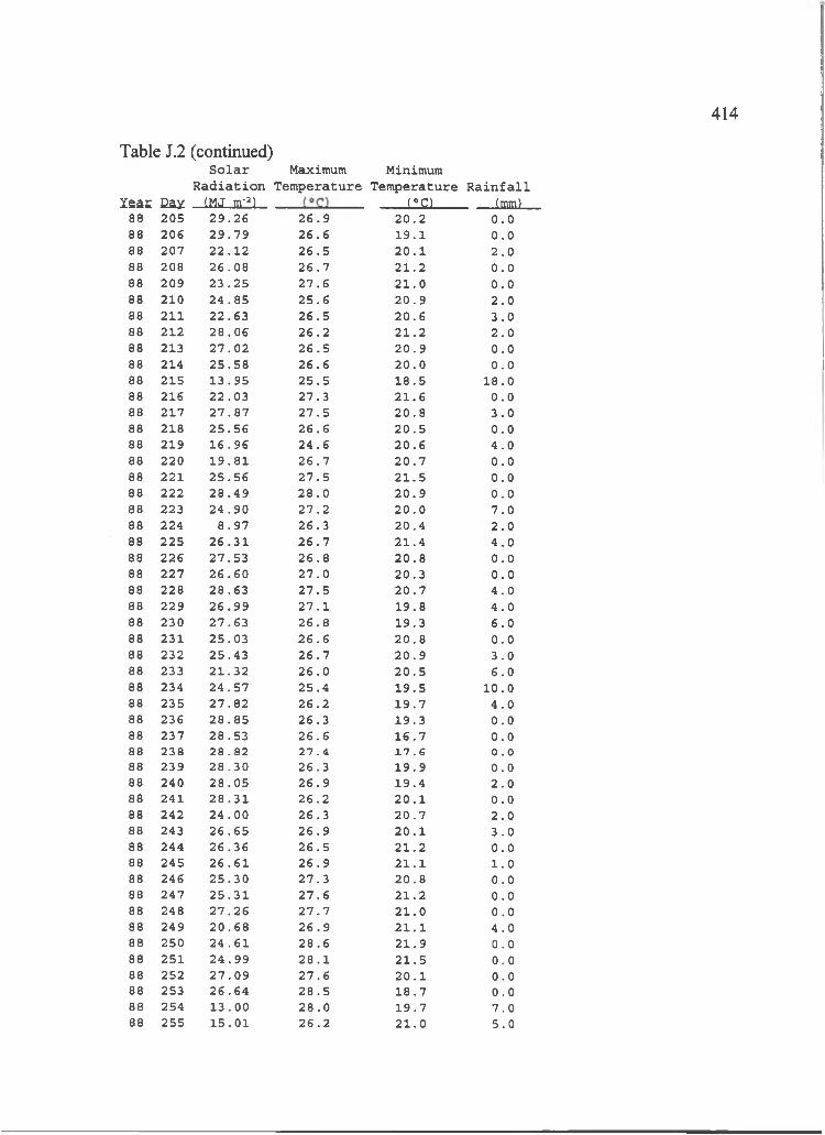
414
Table J,2 (continued)S o l a r Maximum Minimum
R a d i a t i o n Temperatur e Temperature R a i n f a l l Year Cay IMJ nr=‘l _______ (°o _______(mm)
88 2 0 5 2 9 . 2 6 2 6 . 9 2 0 . 2 0 . 088 2 0 6 2 9 . 7 9 2 6 . 6 1 9 . 1 0 . 088 2 0 7 2 2 . 1 2 2 6 . 5 2 0 . 1 2 . 088 2 08 2 6 . 0 8 2 6 . 7 2 1 . 2 0 . 088 2 0 9 2 3 . 2 5 2 7 . 6 2 1 . 0 0 . 088 2 1 0 2 4 . 8 5 2 5 . 6 2 0 . 9 2 . 088 2 1 1 2 2 . 6 3 2 6 . 5 2 0 . 6 3 . 088 2 1 2 2 8 . 0 6 2 6 . 2 2 1 . 2 2 . 088 2 13 2 7 . 0 2 2 6 . 5 2 0 . 9 0 . 088 2 14 2 5 . 5 8 2 6 . 6 2 0 . 0 0 . 088 2 1 5 1 3 . 9 5 2 5 . 5 1 8 . 5 1 8 . 088 2 1 6 2 2 . 0 3 2 7 . 3 2 1 . 6 0 . 088 2 1 7 2 7 . 8 7 2 7 . 5 2 0 . 8 3 . 088 2 1 8 2 5 . 5 6 26 . 6 2 0 . 5 0 . 088 2 1 9 1 6 . 9 6 2 4 . 6 2 0 . 6 4 . 088 2 2 0 1 9 . 8 1 2 6 . 7 2 0 . 7 0 . 088 2 2 1 2 5 . 5 6 2 7 . 5 2 1 . 5 0 . 088 2 2 2 2 8 . 4 9 2 8 . 0 2 0 . 9 0 . 088 2 2 3 2 4 . 9 0 2 7 . 2 2 0 . 0 7 . 088 2 2 4 8 . 9 7 2 6 . 3 2 0 . 4 2 . 088 2 2 5 2 6 . 3 1 2 6 . 7 2 1 . 4 4 . 088 2 2 6 2 7 . 5 3 2 6 . 8 2 0 . 8 0 . 088 2 2 7 2 6 . 6 0 2 7 . 0 2 0 . 3 0 . 088 2 2 8 2 8 . 6 3 2 7 . 5 2 0 . 7 4 . 088 2 2 9 2 6 . 9 9 2 7 . 1 1 9 . 8 4 . 088 2 3 0 2 7 . 6 3 2 6 . 8 1 9 . 3 6 . 088 2 3 1 2 5 . 0 3 2 6 . 6 2 0 . 8 0 . 088 2 3 2 2 5 . 4 3 2 6 . 7 2 0 . 9 3 . 088 2 33 2 1 . 3 2 2 6 . 0 2 0 . 5 6 . 088 2 3 4 2 4 . 5 7 2 5 . 4 1 9 . 5 1 0 . 088 2 3 5 2 7 . 8 2 2 6 . 2 1 9 . 7 4 . 088 2 3 6 2 8 . 8 5 2 6 . 3 1 9 . 3 0 . 088 2 3 7 2 8 . 5 3 2 6 . 6 1 6 . 7 0 . 088 2 3 8 28 . 82 27 . 4 1 7 . 6 0 . 088 2 3 9 28 . 3 0 2 6 . 3 1 9 . 9 0 . 088 2 4 0 2 8 . 0 5 2 6 . 9 1 9 . 4 2 . 088 2 4 1 2 8 . 3 1 2 6 . 2 2 0 . 1 0 . 088 2 4 2 2 4 . 0 0 2 6 . 3 2 0 . 7 2 . 088 2 43 2 6 . 6 5 2 6 . 9 2 0 . 1 3 . 088 2 4 4 2 6 . 3 6 2 6 . 5 2 1 . 2 0 . 088 2 4 5 26 . 6 1 2 6 . 9 2 1 . 1 1 . 088 2 4 6 2 5 . 3 0 2 7 . 3 2 0 . 8 0 . 088 2 4 7 2 5 . 3 1 2 7 . 6 2 1 . 2 0 . 088 2 4 8 2 7 . 2 6 2 7 . 7 2 1 . 0 0 . 088 2 4 9 2 0 . 6 8 2 6 . 9 2 1 . 1 4 . 088 25 0 2 4 . 6 1 2 8 . 6 2 1 . 9 0 . 088 2 5 1 2 4 . 9 9 2 8 . 1 2 1 . 5 0 . 088 25 2 2 7 . 0 9 2 7 . 6 2 0 . 1 0 . 088 253 26 . 6 4 2 8 . 5 1 8 . 7 0 . 088 25 4 1 3 . 0 0 2 8 . 0 1 9 . 7 7 . 088 2 5 5 1 5 . 0 1 2 6 . 2 2 1 . 0 5 . 0
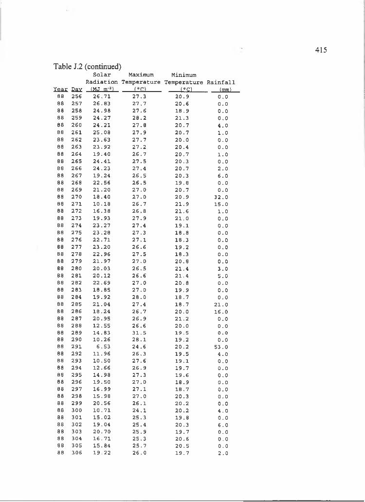
415
Y e a r g a z ( M J _______________________ L l S I l ____ (mm)88 2 5 6 2 6 . 7 1 2 7 . 3 2 0 . 9 0 . 088 2 5 7 2 6 . 8 3 2 7 . 7 2 0 . 6 0 . 088 2 5 8 2 4 . 9 8 2 7 . 6 1 8 . 9 0 . 088 2 5 9 2 4 . 2 7 2 8 . 2 2 1 . 3 0 . 088 2 6 0 2 4 . 2 1 2 7 . 8 2 0 . 7 4 . 088 2 6 1 2 5 . 0 8 2 7 . 9 2 0 . 7 1 . 088 2 6 2 2 3 . 6 3 2 7 . 7 2 0 . 0 0 . 088 26 3 2 3 . 9 2 2 7 . 2 2 0 . 4 0 . 088 2 6 4 1 9 . 4 0 2 6 . 7 2 0 . 7 1 . 088 2 6 5 2 4 . 4 1 2 7 . 5 2 0 . 3 0 . 088 2 6 6 2 4 . 2 3 2 7 . 4 2 0 . 7 2 . 088 2 6 7 1 9 . 2 4 2 6 . 5 2 0 . 3 6 . 088 2 6 8 2 2 . 5 6 2 6 . 5 1 9 . 8 0 . 088 2 6 9 2 1 . 2 0 2 7 . 0 2 0 . 7 0 . 088 2 7 0 1 8 . 4 0 2 7 . 0 2 0 . 9 3 2 . 088 2 7 1 1 0 . 1 8 2 6 . 7 2 1 . 9 1 5 . 088 2 7 2 1 6 . 3 8 2 6 . 8 2 1 . 6 1 . 088 27 3 1 9 . 9 3 2 7 . 9 2 1 . 0 0 . 088 2 7 4 2 3 . 2 7 2 7 . 4 1 9 . 1 0 . 088 2 7 5 2 3 . 2 8 2 7 . 3 1 8 . 8 0 . 088 2 7 6 2 2 . 7 1 2 7 . 1 1 8 . 3 0 . 088 2 7 7 2 3 . 2 0 2 6 . 6 1 9 . 2 0 . 088 2 7 8 2 2 . 9 6 2 7 . 5 1 8 . 3 0 . 088 2 7 9 2 1 . 9 7 2 7 . 0 2 0 . 8 0 . 088 2 8 0 2 0 . 0 3 2 6 . 5 2 1 . 4 3 . 088 2 8 1 2 0 . 1 2 2 6 . 6 2 1 . 4 5 . 088 2 8 2 2 2 . 6 9 2 7 . 0 2 0 . 8 0 . 088 28 3 1 8 . 8 5 2 7 . 0 1 9 . 9 0 . 088 28 4 1 9 . 9 2 2 8 . 0 1 8 . 7 0 . 088 2 8 5 2 1 . 0 4 2 7 . 4 1 8 . 7 2 1 . 088 2 8 6 1 8 . 2 4 2 6 . 7 2 0 . 0 1 6 . 088 2 8 7 2 0 . 9 5 2 6 . 9 2 1 . 2 0 . 088 2 8 8 1 2 . 5 5 2 6 . 6 2 0 . 0 0 . 088 2 8 9 1 4 . 8 3 3 1 . 5 1 9 . 5 0 . 088 2 9 0 1 0 . 2 6 2 8 . 1 1 9 . 2 0 . 088 2 9 1 6 . 5 3 2 4 . 6 2 0 . 2 5 3 . 088 2 9 2 1 1 . 9 6 2 6 . 3 1 9 . 5 4 . 088 29 3 1 0 . 5 0 2 7 . 6 1 9 . 1 0 . 088 2 9 4 1 2 . 6 6 2 6 . 9 1 9 . 7 0 . 088 2 9 5 1 4 . 9 8 2 7 . 3 1 9 . 6 0 . 088 2 9 6 1 9 . 5 0 2 7 . 0 1 8 . 9 0 . 088 2 9 7 1 6 . 9 9 2 7 . 1 1 8 . 7 0 . 088 2 9 8 1 5 . 9 8 2 7 . 0 2 0 . 3 0 . 088 2 9 9 2 0 . 5 6 2 6 . 1 2 0 . 2 0 . 088 3 0 0 1 0 . 7 1 2 4 . 1 2 0 . 2 4 . 088 3 0 1 1 5 . 0 2 2 5 . 3 1 9 . 8 0 . 088 3 0 2 1 9 . 0 4 2 5 . 4 2 0 . 3 6 . 088 30 3 2 0 . 7 0 2 5 . 9 1 9 . 7 0 . 088 3 0 4 1 6 . 7 1 2 5 . 3 2 0 . 6 0 . 088 3 0 5 1 5 . 8 4 2 5 . 7 2 0 . 5 0 . 088 3 0 6 1 9 . 2 2 2 6 . 0 1 9 . 7 2 . 0
Table J.2 (continued)S o l a r Maximum Minimum
R a d i a t i o n T e m p e r a tu r e T e m p e ra tu r e R a i n f a l l
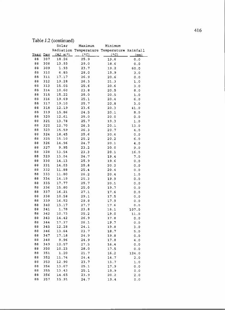
416
X a a r Cay (MJ ___________________ L isn____(mm)88 3 0 7 1 8 . 2 6 2 5 . 9 1 9 . 6 0 . 088 3 0 8 1 3 . 9 3 2 9 . 0 1 8 . 6 0 . 088 3 0 9 1 . 9 3 2 3 . 7 1 9 . 2 6 0 . 088 3 1 0 6 . 8 5 2 8 . 0 1 9 . 9 3 . 088 3 1 1 1 7 . 1 7 2 6 . 9 2 0 . 6 0 . 088 3 1 2 1 9 . 2 8 2 6 . 3 2 1 . 3 1 . 088 31 3 1 5 . 0 5 2 5 . 6 2 0 . 6 3 . 088 3 1 4 1 0 . 6 0 2 3 . 8 2 0 . 5 8 . 088 3 1 5 1 5 . 2 2 2 5 . 0 2 0 . 5 1 . 088 3 1 6 1 9 . 6 9 2 5 . 1 2 0 . 4 6 . 088 3 1 7 1 9 . 1 0 2 5 . 7 2 0 . 8 3 . 088 3 1 8 1 2 . 1 9 2 3 . 6 2 0 . 3 4 1 . 088 3 1 9 1 5 . 8 6 2 4 . 5 2 0 . 1 8 . 088 3 2 0 1 2 . 6 1 2 5 . 0 2 0 . 0 0 . 088 3 2 1 1 3 . 7 8 2 5 . 7 1 9 . 3 1 . 088 3 2 2 1 2 . 7 0 2 6 . 3 2 0 . 1 1 3 . 088 3 2 3 1 5 . 5 9 2 6 . 3 2 0 . 7 4 . 088 3 2 4 1 8 . 4 5 2 5 . 6 2 0 . 6 0 . 088 3 2 5 1 5 . 1 0 2 5 . 2 2 0 . 2 6 . 088 3 2 6 1 4 . 9 6 2 4 . 7 2 0 . 1 4 . 088 3 2 7 9 . 9 5 2 3 . 2 2 0 . 0 9 . 088 3 2 8 1 3 . 5 4 2 3 . 3 2 0 . 1 1 6 . 088 3 2 9 1 3 . 0 4 2 4 . 7 1 9 . 4 7 . 088 3 3 0 1 4 . 1 3 2 5 . 9 1 9 . 6 0 . 088 3 3 1 1 4 . 0 3 2 5 . 8 2 0 . 2 0 . 088 3 3 2 1 1 . 8 8 2 5 . 4 2 0 . 4 0 . 088 3 3 3 1 1 . 8 0 2 6 . 2 2 0 . 4 1 . 088 3 3 4 1 4 . 1 9 2 5 . 3 1 9 . 9 0 . 088 3 3 5 1 7 . 7 7 2 5 . 7 2 0 . 1 0 . 088 3 3 6 1 5 . 8 0 2 5 . 0 1 9 . 7 0 . 088 3 3 7 1 6 . 2 1 2 7 . 1 1 7 . 6 0 . 088 3 3 8 1 0 . 5 8 2 9 . 1 1 7 . 5 0 . 088 3 3 9 1 6 . 5 2 2 9 . 8 1 7 . 9 0 . 088 3 4 0 1 3 . 1 7 2 7 . 7 1 7 . 6 0 . 088 3 4 1 1 . 7 8 2 3 . 8 1 8 . 1 1 0 7 . 088 3 4 2 1 0 . 7 3 2 5 . 2 1 9 . 0 1 1 . 088 3 4 3 1 4 . 4 2 2 6 . 9 1 7 . 8 0 . 088 3 4 4 1 7 . 3 7 2 6 . 1 1 9 . 7 0 . 088 3 4 5 1 2 . 2 8 2 4 . 1 1 9 . 8 3 . 088 3 4 6 1 3 . 6 4 2 3 . 7 1 8 . 7 5 . 088 3 4 7 1 7 . 1 8 2 4 . 9 1 9 . 8 0 . 088 3 4 8 9 . 9 6 2 4 . 9 1 7 . 8 4 . 088 3 4 9 1 2 . 5 7 2 7 . 5 1 6 . 4 0 . 088 3 5 0 1 0 . 2 3 2 8 . 0 1 7 . 5 0 . 088 3 5 1 1 . 2 0 2 1 . 7 1 6 . 2 1 2 4 . 088 3 5 2 1 1 . 7 4 2 4 . 4 1 4 . 7 2 . 088 3 5 3 1 2 . 9 0 2 3 . 7 1 3 . 7 1 . 088 3 5 4 1 3 . 6 7 2 5 . 1 1 7 . 9 0 . 088 3 5 5 1 3 . 4 3 2 5 . 1 1 9 . 9 0 . 088 3 5 6 1 4 . 6 5 2 3 . 9 2 0 . 2 2 . 088 3 5 7 1 5 . 9 1 2 4 . 7 1 9 . 4 0 . 0
Table J.2 (continued)S o l a r Maximum Minimum
R a d i a t i o n T e m p e r a tu r e T e m p e r a tu r e R a i n f a l l
417
Table J.2 (continued)S o l a r Maximum Minimum
R a d i a t i o n Temperatur e Temperature R a i n f a l l Year Cax (MJ m~')___________________ ilsn____(mm)
88 358 1 7 . 5 9 2 4 . 6 1 9 . 6 4 . 088 359 1 3 . 9 1 2 4 . 1 1 9 . 2 9 . 088 360 1 5 . 9 5 2 3 . 9 1 8 . 9 2 3 . 088 361 1 5 . 6 0 2 4 . 3 1 8 .4 3 . 088 362 1 4 . 4 2 2 4 . 3 1 9 . 0 9 . 088 363 9 . 9 3 2 3 . 6 1 9 . 5 9 . 088 364 5 . 7 5 2 1 . 3 1 8 . 7 5 0 . 088 365 6 . 8 9 2 0 . 7 1 8 .3 3 2 . 088 366 9 . 5 4 2 2 . 8 1 9 . 0 1 2 . 089 1 1 5 . 8 8 2 2 . 6 1 8 . 6 8 . 089 2 1 5 .0 3 2 4 . 0 1 7 . 6 1 . 089 3 1 7 .5 3 2 4 . 6 1 8 . 7 4 . 089 4 1 7 . 5 5 2 3 . 5 1 8 .3 0 . 089 5 1 2 . 9 0 2 2 . 7 1 6 . 9 8 . 089 6 1 1 .6 3 2 2 . 8 1 8 . 2 2 6 . 089 7 1 2 . 2 6 2 2 . 1 1 8 . 6 2 9 . 089 8 1 3 . 9 0 2 2 . 8 1 7 .3 1 9 .089 9 1 0 . 4 5 2 1 . 1 1 7 .3 3 3 . 089 10 6 . 0 1 2 2 . 1 1 8 .3 5 4 . 089 11 6 . 5 7 2 4 . 1 1 9 . 0 2 3 . 089 12 1 2 . 8 7 2 5 . 0 1 8 . 6 2 2 . 089 13 5 . 9 8 2 1 . 3 1 8 . 9 2 1 . 089 14 9 . 6 3 2 0 . 3 1 8 . 7 1 9 . 089 15 1 2 . 2 8 2 1 . 2 1 8 . 3 1 9 . 089 16 1 6 .4 3 2 3 . 2 1 8 . 5 5 . 089 17 1 8 . 2 9 2 3 . 5 1 8 . 3 2 . 089 18 1 6 .5 3 2 3 . 3 1 8 . 1 0 . 089 19 1 7 . 4 1 2 3 . 4 1 8 .3 2 6 . 089 20 1 6 . 2 0 2 4 . 0 1 7 . 9 2 . 089 21 1 6 . 2 2 2 3 . 7 1 7 . 5 2 . 089 22 1 8 . 1 5 2 3 . 6 1 8 . 0 1 . 089 23 1 2 .2 3 2 3 . 7 1 8 . 4 0 . 089 24 1 7 . 6 1 2 7 . 9 1 6 .4 0 . 089 25 1 6 . 2 5 2 4 . 9 1 6 . 6 0 . 089 26 1 8 . 4 4 2 3 . 8 1 7 . 6 1 . 089 27 1 8 . 5 6 2 4 . 5 1 6 . 7 0 . 089 28 1 8 . 4 6 2 8 . 3 1 4 . 6 0 . 089 29 5 . 4 9 2 4 . 3 1 7 .3 1 7 . 089 30 1 0 .1 3 2 4 . 1 1 6 . 0 0 . 089 31 6 . 8 5 2 3 . 3 1 6 . 9 0 . 089 32 1 4 . 6 9 2 7 . 5 1 5 . 8 0 . 089 33 1 7 . 4 5 2 7 . 3 1 6 . 4 1 2 . 089 34 5 . 0 3 1 9 . 7 1 6 . 5 5 1 . 089 35 2 . 5 3 1 9 . 2 1 5 . 7 1 7 8 .089 36 1 5 . 0 6 2 4 . 7 1 7 . 1 0 . 089 37 1 2 . 4 5 2 5 . 3 1 7 . 7 3 . 089 38 1 1 . 7 5 2 6 . 6 1 8 . 6 1 . 089 39 1 8 . 3 9 2 7 . 8 1 8 . 7 0 .089 40 1 6 . 7 1 2 8 . 0 1 6 .3 3 . 089 41 8 . 9 8 2 3 . 2 1 9 .3 1 . 089 42 7 . 1 7 2 4 . 9 1 5 . 5 2 1 . 0
418
Table J.2 (continued)S o l a r Maximum Minimum
R a d i a t i o n Temperat ure Temperature R a i n f a l lX a a r Cay (MJ ________( ° o ( ° o __________ (mm)
89 43 1 2 . 6 0 2 7 . 8 1 6 . 7 0 . 089 44 1 8 . 0 8 2 9 . 2 1 6 . 2 0 . 089 45 1 7 . 6 5 2 5 . 0 1 6 . 3 0 .089 46 1 5 . 7 6 2 6 . 0 1 6 . 3 0 . 089 47 2 0 . 6 9 2 5 . 2 1 5 . 4 0 . 089 48 2 1 . 7 5 2 5 . 2 1 7 . 4 0 . 089 49 2 1 . 4 5 2 4 . 6 1 8 . 6 0 . 089 50 2 1 . 2 9 2 4 . 1 1 7 . 6 1 . 089 51 2 0 . 8 2 2 4 . 2 1 7 . 5 0 . 089 52 2 1 . 3 9 2 4 . 3 1 7 . 9 3 . 089 53 1 3 . 3 5 2 2 . 3 1 8 .3 2 . 089 54 1 2 .7 3 2 2 . 6 1 8 . 5 1 4 .089 55 1 8 . 6 4 2 2 . 8 1 7 . 2 2 . 089 56 2 1 . 4 0 2 2 . 3 1 6 . 9 3 . 089 57 2 3 . 0 1 2 3 . 1 1 6 . 9 0 . 089 58 9 . 3 1 2 6 . 5 1 5 .4 0 . 089 59 5 . 4 5 2 3 . 2 1 7 . 7 8 . 089 60 1 0 . 2 0 2 6 . 7 1 7 . 3 5 . 089 61 1 7 . 2 7 2 7 . 0 2 1 . 9 3 . 089 62 1 7 .0 4 2 8 . 2 2 2 . 0 4 . 089 63 6 . 0 8 2 4 . 4 1 9 . 0 5 0 . 089 64 7 . 9 4 2 1 . 4 1 8 . 5 6 . 089 65 6 . 7 4 2 0 . 9 1 8 . 7 2 7 . 089 66 1 7 . 0 7 2 3 . 3 1 6 . 9 1 7 . 089 67 1 6 . 9 9 2 2 . 1 1 5 . 9 0 . 089 68 1 9 . 0 9 2 2 . 9 1 4 . 3 0 . 089 69 2 2 . 3 1 2 3 . 4 1 6 . 5 0 . 089 70 2 0 . 3 7 2 3 . 6 1 4 . 0 0 . 089 71 1 9 . 0 6 2 4 . 2 1 8 . 1 4 . 089 72 2 4 . 8 5 2 4 . 4 1 6 . 8 0 . 089 73 2 5 . 3 2 2 3 . 9 1 7 . 9 0 . 089 74 1 4 . 7 9 2 4 . 5 1 8 . 9 0 . 089 75 1 7 . 9 0 2 7 . 8 1 6 . 8 0 . 089 76 1 8 . 5 4 2 8 . 3 1 6 .3 0 . 089 77 2 1 . 4 2 2 7 . 2 1 6 . 6 0 . 089 78 1 6 . 9 2 2 6 . 3 1 7 .4 0 . 089 79 2 1 . 1 3 2 6 . 1 1 6 . 6 0 . 089 80 2 5 . 0 0 2 5 . 6 1 8 . 9 0 . 089 81 2 5 . 4 6 2 5 . 0 1 9 . 2 0 . 089 82 2 5 . 6 9 2 4 . 8 1 9 . 2 0 . 089 83 2 4 . 1 7 2 5 . 3 1 9 . 2 3 . 089 84 2 3 . 0 3 2 6 . 9 1 9 .4 0 . 089 85 1 7 . 4 6 2 7 . 6 1 7 . 7 0 . 089 86 2 6 . 2 6 2 5 . 5 1 6 . 8 0 . 089 87 2 5 . 1 4 2 5 . 7 1 9 .4 1 .089 88 2 3 . 4 3 2 4 . 8 1 9 . 1 8 .089 89 1 7 . 1 6 2 3 . 6 1 9 . 2 1 .089 90 1 5 . 7 7 2 3 . 4 1 8 . 7 3 7 . 089 91 2 2 . 7 5 2 4 . 0 1 8 . 7 1 3 .089 92 1 9 . 5 8 2 4 . 7 1 8 . 6 2 5 . 089 93 1 5 . 0 9 2 6 . 7 1 6 . 9 7 . 0
419
Ysac Eay m- 1_____________ ( ° 0 ____(mm)89 94 1 5 . 1 2 2 8 . 089 95 6 . 1 8 1 9 . 589 96 7 . 2 2 1 9 . 089 97 1 . 8 4 1 7 . 589 98 3 . 8 6 1 9 . 089 99 1 4 . 2 6 2 1 . 989 100 1 5 . 4 3 2 3 . 289 101 2 3 . 3 0 2 3 . 889 102 1 3 . 2 7 2 3 . 589 103 1 0 . 0 3 2 2 . 389 104 8 . 3 9 1 8 .889 105 8 . 0 0 1 9 . 889 106 6 . 4 3 2 0 . 589 107 1 2 . 7 3 2 1 . 889 108 1 9 . 9 7 2 2 . 689 109 2 4 . 8 6 2 3 . 789 110 1 4 . 6 0 2 0 . 689 111 1 9 . 3 0 2 3 . 589 112 2 5 . 4 2 2 4 . 389 113 1 1 . 5 1 2 2 . 189 114 2 3 . 5 5 2 5 . 189 115 2 1 . 3 2 2 3 . 589 116 2 2 . 7 8 2 4 . 789 117 1 1 . 5 9 2 2 . 289 118 9 . 7 1 2 1 . 889 119 8 . 1 1 2 0 . 789 120 1 2 . 0 1 2 3 . 589 121 2 0 . 7 2 2 4 . 989 122 1 4 . 9 5 2 4 . 289 123 1 1 . 2 2 2 1 . 889 124 1 9 . 2 8 2 3 . 289 125 2 2 . 7 3 2 3 . 289 126 1 9 .6 3 2 4 . 889 127 2 2 . 0 4 2 4 . 689 128 2 3 . 1 7 2 5 . 289 129 1 3 . 1 1 2 3 . 989 130 2 4 . 3 3 2 5 . 689 131 2 2 . 2 0 2 5 . 389 132 2 6 . 4 3 2 5 . 689 133 2 1 . 2 1 2 4 . 989 134 1 5 . 7 7 2 3 . 489 135 2 0 . 6 8 2 5 . 089 136 2 0 . 5 6 2 4 . 589 137 2 2 . 3 9 2 4 . 389 138 2 6 . 8 7 2 5 . 489 139 2 0 . 1 9 2 3 . 689 140 2 4 . 5 5 2 5 . 289 141 2 3 . 5 1 2 5 . 789 142 1 5 . 2 6 2 4 . 189 143 1 9 . 4 7 2 4 . 889 144 2 1 . 6 7 2 5 . 0
Table J.2 (continued)■ S o l a r Maximum Minimum
R a d i a t i o n T e m p e r a tu r e T e m p e ra tu r e R a i n f a l l
1 6 .2 2 . 01 6 .2 14 9 .016 .1 9 1 . 01 5 . 9 2 2 4 . 016 .5 13 1 .01 6 . 5 12 7 .01 5 .6 2 . 01 5 .3 0 . 01 7 . 9 6 . 01 8 . 5 2 1 . 01 6 .6 54 .016 .3 0 . 01 7 . 1 0 . 01 6 . 9 0 . 01 7 .2 0 . 01 7 . 7 1 . 01 7 . 9 5 2 . 018 .3 3 . 01 8 . 7 4 . 019 .3 3 3 . 01 9 . 6 1 . 01 7 . 8 8 . 01 6 . 1 6 . 01 7 . 5 2 2 . 01 8 .2 3 5 . 01 7 .8 7 1 . 01 7 . 5 6 . 01 6 . 5 0 . 01 6 .8 0 . 01 5 .4 4 . 01 7 .2 0 . 01 8 .4 0 . 018 .3 1 . 018 . 8 2 . 01 9 .2 0 . 02 0 . 2 0 . 01 9 . 7 1 . 01 9 .4 1 . 01 9 . 7 1 . 01 9 . 7 6 . 01 9 . 7 8 .01 9 . 7 1 2 . 01 9 . 5 1 .01 9 . 7 0 . 01 8 . 7 2 . 01 9 . 1 6 . 01 9 . 7 7 . 01 9 .6 6 . 018 .8 46 .01 9 . 7 1 5 .01 9 .9 6 . 0
420
Xsai; Cay (mj m- )________(°o (°o__________ (mm)89 145 1 4 . 9 9 2 3 . 9 1 9 . 8 2 . 089 146 2 3 . 7 3 2 5 . 6 2 0 . 0 1 . 089 147 2 5 . 2 4 2 6 . 6 2 1 . 0 3 . 089 148 2 1 . 5 2 2 5 . 4 2 0 . 4 0 . 089 149 1 7 . 7 7 2 4 . 7 1 9 . 7 3 . 089 150 1 9 . 1 2 2 4 . 3 1 9 . 2 3 5 . 089 151 1 3 . 2 9 2 4 . 5 1 9 .3 3 . 089 152 2 7 . 7 2 2 6 . 4 1 9 .3 0 . 089 153 2 8 . 6 7 2 6 . 3 1 8 . 9 0 . 089 154 2 7 . 1 2 2 6 . 0 2 0 . 6 1 0 .089 155 1 8 . 0 4 2 4 . 5 2 0 . 2 5 . 089 156 2 2 . 7 2 2 5 . 0 1 9 . 5 8 .089 157 2 0 . 3 6 2 4 . 7 2 0 . 1 4 . 089 158 1 9 . 0 6 2 4 . 6 1 9 . 7 1 . 089 159 1 9 . 5 9 2 5 . 2 1 9 . 8 2 . 089 160 2 5 . 8 2 2 5 . 2 2 0 . 5 0 . 089 161 1 4 . 2 2 2 4 . 7 1 9 . 9 0 . 089 162 2 3 . 3 8 2 4 . 8 1 9 . 0 2 . 089 163 1 5 . 5 5 2 2 . 3 1 9 . 7 1 1 . 089 164 2 5 . 0 7 2 5 . 0 1 8 . 6 4 . 089 165 2 0 . 6 0 2 4 . 5 1 9 . 2 0 . 089 166 1 8 . 4 9 2 4 . 5 1 9 . 6 1 1 . 089 167 1 6 . 0 6 2 5 . 3 2 0 . 2 1 6 . 089 168 1 2 . 4 8 2 3 . 2 1 9 . 9 2 7 . 089 169 2 6 . 8 8 2 5 . 9 2 0 . 0 2 . 089 170 2 5 . 6 2 2 6 . 2 1 9 . 9 1 .089 171 1 7 . 9 6 2 4 . 7 2 0 . 1 6 . 089 172 2 5 . 8 8 2 6 . 7 1 9 . 4 0 . 089 173 2 7 . 2 6 2 6 . 7 1 9 . 1 0 . 089 174 2 7 . 9 8 2 5 . 9 1 9 . 8 0 . 089 175 2 4 . 7 7 2 5 . 7 1 9 . 7 0 . 089 176 2 5 . 4 6 2 4 . 9 1 9 . 4 1 . 089 177 1 9 . 9 2 2 6 . 1 1 8 . 6 0 . 089 178 2 2 . 8 0 2 5 . 5 1 9 . 8 0 . 089 179 2 5 . 1 5 2 5 . 8 1 9 . 7 3 . 089 180 2 2 . 3 2 2 5 . 5 1 9 . 8 3 . 089 181 2 2 . 0 8 2 5 . 2 1 9 . 9 1 1 .089 182 2 2 . 0 5 2 5 . 2 1 9 . 9 4 . 089 183 2 5 . 4 0 2 5 . 6 1 9 . 7 3 . 089 184 2 2 . 2 8 2 5 . 4 1 9 . 6 8 .089 185 2 5 . 5 2 2 5 . 3 1 9 . 8 1 9 . 089 186 2 7 . 4 5 2 5 . 8 1 9 . 5 2 6 . 089 187 1 9 . 0 0 2 4 . 5 1 9 . 5 2 1 . 089 188 2 7 . 5 4 2 5 . 7 1 9 . 9 0 . 089 189 2 6 . 1 2 2 5 . 6 2 0 . 1 1 . 089 190 2 2 . 2 6 2 6 . 1 2 0 . 6 4 . 089 191 2 1 . 9 1 2 5 . 9 2 0 . 6 2 3 . 089 192 2 5 . 8 5 2 5 . 9 2 0 . 3 4 . 089 193 2 1 . 2 8 2 5 . 3 2 0 . 1 7 . 089 194 1 7 . 9 9 2 4 . 2 1 9 . 9 3 9 . 089 195 2 3 . 5 4 2 5 . 3 2 0 . 3 9 . 0
Table J.2 (continued)S o l a r Maximum Minimum
R a d i a t i o n T e m p e r a tu r e T e m p e r a tu r e R a i n f a l l
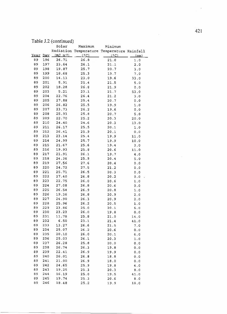
421
Year Cay -OaJ m' )______________ ( ° o ____(mm)89 19S 2 6 . 7 1 2 6 . 8 2 1 . 0 1 . 089 197 2 3 . 6 4 2 6 . 1 2 1 . 1 2 . 089 198 1 9 . 8 7 2 5 . 7 2 0 . 7 3 . 089 199 1 8 . 6 8 2 5 . 3 1 9 . 7 7 . 089 200 1 4 . 1 3 2 3 . 0 1 9 . 6 3 3 . 089 201 5 . 9 1 2 5 . 4 2 1 . 5 5 . 089 202 1 8 . 2 8 2 6 . 8 2 1 . 9 0 . 089 203 5 . 2 1 2 3 . 1 2 1 . 7 5 3 . 089 204 2 2 . 7 6 2 6 . 4 2 1 . 2 3 . 089 205 2 7 . 8 8 2 5 . 4 2 0 . 7 0 . 089 206 2 6 . 8 2 2 5 . 5 1 9 . 9 1 . 089 207 2 3 . 7 3 2 6 . 2 1 9 . 6 0 . 089 208 2 5 . 9 3 2 5 . 8 2 0 . 7 5 . 089 209 2 2 . 7 0 2 5 . 2 2 0 . 3 2 0 . 089 210 2 4 . 4 0 2 4 . 6 2 0 . 3 1 3 . 089 211 2 6 . 1 7 2 5 . 5 2 0 . 1 1 . 089 212 2 6 . 4 1 2 5 . 9 2 0 . 1 0 . 089 213 2 3 . 1 4 2 5 . 4 1 9 . 9 1 1 . 089 214 2 4 . 9 9 2 5 . 7 1 9 . 9 1 0 . 089 215 2 1 . 6 7 2 5 . 6 1 9 . 4 3 . 089 216 1 9 . 9 3 2 5 . 8 2 0 . 6 1 1 . 089 217 2 1 . 9 1 2 6 . 1 1 9 . 7 4 . 089 218 2 4 . 3 6 2 5 . 9 2 0 . 4 5 . 089 219 2 7 . 5 6 2 7 . 6 2 0 . 4 0 . 089 220 2 4 . 7 2 2 7 . 5 2 1 . 2 0 . 089 221 2 5 . 7 1 2 6 . 5 2 0 . 3 0 . 089 222 2 7 . 4 0 2 6 . 8 2 0 . 2 0 . 0 .89 223 2 2 . 7 5 2 6 . 0 2 0 . 6 1 .089 224 2 7 . 0 8 2 6 . 8 2 0 . 6 0 . 089 225 2 6 . 5 4 2 6 . 9 2 0 . 8 1 .089 226 1 9 . 3 6 2 6 . 8 2 0 . 9 2 . 089 227 2 4 . 9 0 2 6 . 3 2 0 . 9 2 . 089 228 2 5 . 9 6 2 6 . 2 2 0 . 5 1 .089 229 2 3 . 8 6 2 5 . 0 2 0 . 1 5 . 089 230 2 3 . 2 3 2 6 . 0 1 9 . 8 0 . 089 231 1 1 . 7 8 2 5 . 8 2 1 . 0 1 4 .089 232 6 . 5 0 2 3 . 1 2 1 . 4 4 1 . 089 233 1 3 . 2 7 2 6 . 6 2 1 . 5 7 . 089 234 2 5 . 0 7 2 6 . 2 2 0 . 6 0 . 089 235 2 0 . 1 0 2 6 . 0 2 0 . 1 6 . 089 236 2 5 . 0 3 2 6 . 1 2 0 . 3 1 .089 237 2 6 . 2 8 2 5 . 8 2 0 . 0 0 . 089 238 2 6 . 7 4 2 6 . 3 1 9 . 8 0 . 089 239 2 2 . 4 1 2 6 . 9 1 9 . 9 0 . 089 240 2 6 . 0 1 2 6 . 8 1 8 . 8 0 . 089 241 2 1 . 0 0 2 6 . 9 1 8 . 0 0 . 089 242 2 4 . 6 5 2 5 . 9 1 9 . 8 4 . 089 243 1 9 . 2 5 2 5 . 3 2 0 . 3 8 .089 244 1 6 . 1 9 2 5 . 0 1 9 . 5 4 1 . 089 245 1 9 .7 4 2 5 . 3 2 0 . 6 8 .089 246 1 8 . 4 8 2 5 . 2 1 9 . 9 1 8 .0
Table J.2 (continued)S o l a r Maximum Minimum
R a d i a t i o n T e m p e r a tu r e T e m p e r a tu r e R a i n f a l l
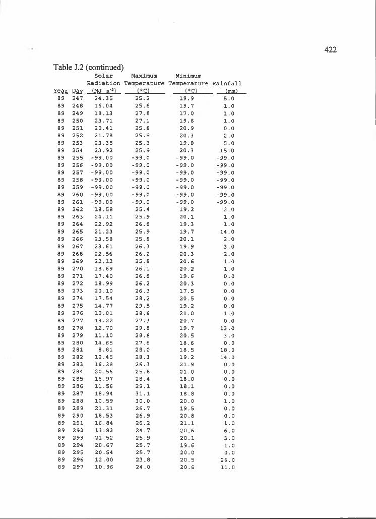
422
Year Cay (MJ nr ) _______ (mm)89 247 2 4 . 3 5 2 5 . 2 1 9 . 9 5 . 089 248 1 6 . 0 4 2 5 . 6 1 9 . 7 1 . 089 249 1 8 .1 3 2 7 . 8 1 7 . 0 1 . 089 250 2 3 . 7 1 2 7 . 1 1 9 .8 1 . 089 251 2 0 . 4 1 2 5 . 8 2 0 . 9 0 . 089 252 2 1 . 7 8 2 5 . 5 2 0 . 3 2 . 089 253 2 3 . 3 5 2 5 . 3 1 9 . 8 5 . 089 254 2 3 . 9 2 2 5 . 9 2 0 . 3 1 5 .089 255 - 9 9 . 0 0 - 9 9 . 0 - 9 9 . 0 - 9 9 . 089 256 - 9 9 . 0 0 - 9 9 . 0 - 9 9 . 0 - 9 9 . 089 257 - 9 9 . 0 0 - 9 9 . 0 - 9 9 . 0 - 9 9 . 089 258 - 9 9 . 0 0 - 9 9 . 0 - 9 9 . 0 - 9 9 . 089 259 - 9 9 . 0 0 - 9 9 . 0 - 9 9 . 0 - 9 9 . 089 260 - 9 9 . 0 0 - 9 9 . 0 - 9 9 . 0 - 9 9 . 089 261 - 9 9 . 0 0 - 9 9 . 0 - 9 9 . 0 - 9 9 . 089 262 1 8 . 5 8 2 5 . 4 1 9 . 2 2 . 089 263 2 4 . 1 1 2 5 . 9 2 0 . 1 1 . 089 264 2 2 . 9 2 2 6 . 6 1 9 .3 1 . 089 265 2 1 . 2 3 2 5 . 9 1 9 . 7 1 4 . 089 266 2 3 . 5 8 2 5 . 8 2 0 . 1 2 . 089 267 2 3 . 6 1 2 6 . 3 1 9 . 9 3 . 089 268 2 2 . 5 6 2 6 . 2 2 0 . 3 2 . 089 269 2 2 . 1 2 2 5 . 8 2 0 . 6 1 . 089 270 1 8 . 6 9 2 6 . 1 2 0 . 2 1 . 089 271 1 7 . 4 0 2 6 . 6 1 9 . 6 0 . 089 272 1 8 . 9 9 2 6 . 2 2 0 . 3 0 . 089 273 2 0 . 1 0 2 6 . 3 1 7 . 5 0 . 089 274 1 7 . 5 4 2 8 . 2 2 0 . 5 0 . 089 275 1 4 . 7 7 2 9 . 5 1 9 . 2 0 . 089 276 1 0 . 0 1 2 8 . 6 2 1 . 0 1 . 089 277 1 3 . 2 2 2 7 . 3 2 0 . 7 0 . 089 278 1 2 . 7 0 2 9 . 8 1 9 . 7 1 3 .089 279 1 1 . 1 0 2 8 . 8 2 0 . 5 3 . 089 280 1 4 . 6 5 2 7 . 6 1 8 . 6 0 . 089 281 8 . 8 1 2 8 . 0 1 8 . 5 1 8 . 089 282 1 2 . 4 5 2 8 . 3 1 9 . 2 1 4 . 089 283 1 6 . 2 8 2 6 . 3 2 1 . 9 0 . 089 284 2 0 . 5 6 2 5 . 8 2 1 . 0 0 . 089 285 1 6 . 9 7 2 8 . 4 1 8 . 0 0 . 089 286 1 1 . 5 6 2 9 . 1 1 8 . 1 0 . 089 287 1 8 . 9 4 3 1 . 1 1 8 . 8 0 .089 288 1 0 . 5 9 3 0 . 0 2 0 . 0 1 .089 289 2 1 . 3 1 2 6 . 7 1 9 . 5 0 . 089 290 1 8 .5 3 2 6 . 9 2 0 . 8 0 . 089 291 1 6 . 8 4 2 6 . 2 2 1 . 1 1 .089 292 1 3 . 8 3 2 4 . 7 2 0 . 6 6 . 089 293 2 1 . 5 2 2 5 . 9 2 0 . 1 3 . 089 294 2 0 . 6 7 2 5 . 7 1 9 . 6 1 . 089 295 2 0 . 5 4 2 5 . 7 2 0 . 0 0 . 089 296 1 2 . 0 0 2 3 . 8 2 0 . 5 2 6 . 089 297 1 0 . 9 6 2 4 . 0 2 0 . 6 1 1 .0
Table J.2 (continued)S o l a r Maximum Minimum
R a d i a t i o n T e m p e r a tu r e T e m p e r a tu r e R a i n f a l l
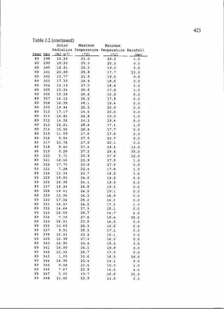
423
S o l a r Maximum Minimum R a d i a t i o n Temperatur e Temperature R a i n f a l l
X s a r Cay (MJ m~")________( ° o ( ° o __________ (mm)89 298 1 6 . 2 6 2 5 . 0 2 0 . 2 1 . 089 299 1 9 . 2 0 2 5 . 3 2 0 . 3 0 . 089 300 1 8 . 8 1 2 5 . 3 1 9 . 0 3 . 089 301 2 0 . 8 9 2 5 . 8 1 7 . 7 2 3 . 089 302 1 0 . 7 7 2 5 . 9 1 9 . 2 0 . 089 303 1 7 . 3 0 2 9 . 9 1 8 . 6 0 . 089 304 1 2 . 1 5 2 7 . 0 1 8 .4 0 . 089 305 1 3 . 2 4 2 6 . 5 1 7 . 9 1 . 089 306 1 8 . 3 9 2 6 . 6 1 6 . 2 0 . 089 307 1 6 . 1 2 2 6 . 5 1 7 . 5 0 . 089 308 1 6 . 9 5 2 8 . 1 1 9 .4 0 . 089 309 1 9 . 4 4 2 5 . 5 2 0 . 9 0 . 089 310 1 7 . 1 7 2 4 . 6 2 0 . 5 0 . 089 311 1 8 . 8 2 2 4 . 8 1 9 . 0 1 . 089 312 1 4 . 2 6 2 4 . 3 1 9 .4 5 . 089 313 1 4 . 6 1 2 8 . 4 1 7 . 1 1 . 089 314 1 5 . 5 6 2 8 . 4 1 7 . 7 0 . 089 315 1 1 . 6 9 2 7 . 6 1 7 . 6 0 . 089 316 9 . 5 4 2 7 . 5 1 9 . 7 0 . 089 317 1 0 . 7 8 2 7 . 6 2 0 . 1 0 . 089 318 8 . 4 0 2 7 . 4 1 9 . 4 1 2 . 089 319 9 . 2 8 2 7 . 2 1 9 .4 3 5 . 089 320 3 . 7 1 2 0 . 9 1 7 . 6 1 2 . 089 321 1 4 . 5 6 2 2 . 9 1 7 . 9 1 . 089 322 1 7 .7 3 2 3 . 8 1 7 . 9 0 . 089 323 7 . 3 8 2 2 . 4 1 7 . 8 1 . 089 324 1 3 . 3 4 2 3 . 7 1 8 . 2 3 . 089 325 1 5 . 8 9 2 4 . 0 1 9 . 2 5 . 089 326 1 6 . 9 5 2 4 . 1 1 9 . 9 0 . 089 327 1 8 . 3 4 2 4 . 5 1 9 .3 0 . 089 328 1 8 . 4 1 2 4 . 5 1 9 . 1 0 . 089 329 1 2 . 9 5 2 4 . 2 1 6 . 9 0 . 089 330 1 7 . 3 4 2 5 . 2 1 6 .3 0 . 089 331 1 8 . 5 7 2 4 . 5 1 7 .3 1 . 089 332 1 4 .6 4 2 7 . 9 1 5 . 1 0 . 089 333 1 6 . 0 9 2 8 . 7 1 6 . 7 4 . 089 334 7 . 3 9 2 7 . 6 1 8 . 4 2 8 . 089 335 1 6 . 9 1 2 3 . 5 1 6 . 5 0 . 089 336 1 5 . 6 9 2 5 . 3 1 6 . 6 0 . 089 337 9 . 3 1 2 5 . 2 1 7 . 1 0 . 089 338 1 6 .2 3 2 5 . 2 1 6 . 1 0 . 089 339 1 2 . 9 5 2 7 . 2 1 6 .3 0 . 089 340 1 6 . 9 6 2 5 . 4 1 5 . 2 0 . 089 341 1 6 . 8 9 2 6 . 0 1 9 . 9 0 . 089 342 1 2 .5 3 2 6 . 7 1 7 . 0 0 . 089 343 1 . 0 5 2 2 . 6 1 6 . 9 5 9 . 089 344 1 4 . 9 5 2 2 . 4 1 4 . 1 0 . 089 345 9 . 5 8 2 3 . 5 1 5 . 0 1 .089 346 7 . 6 7 2 3 . 8 1 6 . 2 4 . 089 347 3 . 5 5 1 9 . 7 1 6 . 6 3 1 . 089 348 1 2 . 4 6 2 2 . 9 1 4 . 6 0 .0
Table J.2 (continued)
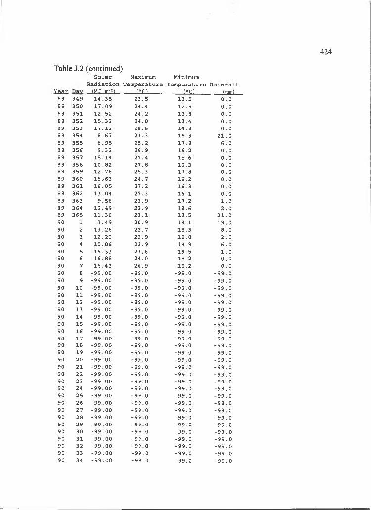
424
Year ..(MJ m-') m Lisn_______ (mm)89 349 1 4 . 3 5 2 3 . 5 1 3 . 5 0 . 089 350 1 7 . 0 9 2 4 . 4 1 2 . 9 0 . 089 351 1 2 . 5 2 2 4 . 2 1 3 . 8 0 . 089 352 1 5 . 3 2 2 4 . 0 1 3 . 4 0 . 089 353 1 7 . 1 2 2 8 . 6 1 4 . 8 0 . 089 354 8 . 6 7 2 3 . 3 1 8 .3 2 1 . 089 355 6 . 9 5 2 5 . 2 1 7 . 8 6 . 089 356 9 . 3 2 2 6 . 9 1 6 . 2 0 . 089 357 1 5 . 1 4 2 7 . 4 1 5 . 6 0 . 089 358 1 0 . 8 2 2 7 . 8 1 6 .3 0 . 089 359 1 2 . 7 6 2 5 . 3 1 7 . 8 0 . 089 360 1 5 .6 3 2 4 . 7 1 6 . 2 0 . 089 361 1 6 . 0 5 2 7 . 2 1 6 .3 0 . 089 362 1 3 . 0 4 2 7 . 3 1 6 . 1 0 . 089 363 9 . 5 6 2 3 . 9 1 7 . 2 1 . 089 364 1 2 . 4 9 2 2 . 9 1 8 . 6 2 . 089 365 1 1 . 3 6 2 3 . 1 1 8 . 5 2 1 . 090 1 3 . 4 9 2 0 . 9 1 8 . 1 1 9 . 090 2 1 3 . 2 6 2 2 . 7 1 8 . 3 8 . 090 3 1 2 . 2 0 2 2 . 9 1 9 . 0 2 . 090 4 1 0 . 0 6 2 2 . 9 1 8 . 9 6 . 090 5 1 6 . 3 3 2 3 . 6 1 9 . 5 1 . 090 6 1 6 . 8 8 2 4 . 0 1 8 . 2 0 . 090 7 1 6 . 4 3 2 6 . 9 1 6 . 2 0 . 090 8 - 9 9 . 0 0 - 9 9 . 0 - 9 9 . 0 - 9 9 . 090 9 - 9 9 . 0 0 - 9 9 . 0 - 9 9 . 0 - 9 9 . 090 10 - 9 9 . 0 0 - 9 9 . 0 - 9 9 . 0 - 9 9 . 090 11 - 9 9 . 0 0 - 9 9 . 0 - 9 9 . 0 - 9 9 . 090 12 - 9 9 . 0 0 - 9 9 . 0 - 9 9 . 0 - 9 9 . 090 13 - 9 9 . 0 0 - 9 9 . 0 - 9 9 . 0 - 9 9 . 090 14 - 9 9 . 0 0 - 9 9 . 0 - 9 9 . 0 - 9 9 . 090 15 - 9 9 . 0 0 - 9 9 . 0 - 9 9 . 0 - 9 9 . 090 16 - 9 9 . 0 0 - 9 9 . 0 - 9 9 . 0 - 9 9 . 090 17 - 9 9 . 0 0 - 9 9 . 0 - 9 9 . 0 - 9 9 . 090 18 - 9 9 . 0 0 - 9 9 . 0 - 9 9 . 0 - 9 9 . 090 19 - 9 9 . 0 0 - 9 9 . 0 - 9 9 . 0 - 9 9 . 090 20 - 9 9 . 0 0 - 9 9 . 0 - 9 9 . 0 - 9 9 . 090 21 - 9 9 . 0 0 - 9 9 . 0 - 9 9 . 0 - 9 9 . 090 22 - 9 9 . 0 0 - 9 9 . 0 - 9 9 . 0 - 9 9 . 090 23 - 9 9 . 0 0 - 9 9 . 0 - 9 9 . 0 - 9 9 . 090 24 - 9 9 . 0 0 - 9 9 . 0 - 9 9 . 0 - 9 9 . 090 25 - 9 9 . 0 0 - 9 9 . 0 - 9 9 . 0 - 9 9 . 090 26 - 9 9 . 0 0 - 9 9 . 0 - 9 9 . 0 - 9 9 . 090 27 - 9 9 . 0 0 - 9 9 . 0 - 9 9 . 0 - 9 9 . 090 28 - 9 9 . 0 0 - 9 9 . 0 - 9 9 . 0 - 9 9 . 090 29 - 9 9 . 0 0 - 9 9 . 0 - 9 9 . 0 - 9 9 . 090 30 - 9 9 . 0 0 - 9 9 . 0 - 9 9 . 0 - 9 9 . 090 31 - 9 9 . 0 0 - 9 9 . 0 - 9 9 . 0 - 9 9 . 090 32 - 9 9 . 0 0 - 9 9 . 0 - 9 9 . 0 - 9 9 . 090 33 - 9 9 . 0 0 - 9 9 . 0 - 9 9 . 0 - 9 9 . 090 34 - 9 9 . 0 0 - 9 9 . 0 - 9 9 . 0 - 9 9 . 0
Table J.2 (continued)S o l a r Maximum Minimum
R a d i a t i o n T e m p e r a tu r e T e m p e ra tu r e R a i n f a l l
425
Year Cay . (MJ nr ) (I£l (°o_______ (mm)90 35 - 9 9 . 0 0 - 9 9 . 0 - 9 9 . 0 - 9 9 . 090 36 - 9 9 . 0 0 - 9 9 . 0 - 9 9 . 0 - 9 9 . 090 37 - 9 9 . 0 0 - 9 9 . 0 - 9 9 . 0 - 9 9 . 090 38 - 9 9 . 0 0 - 9 9 . 0 - 9 9 . 0 - 9 9 . 090 39 - 9 9 . 0 0 - 9 9 . 0 - 9 9 . 0 - 9 9 . 090 40 - 9 9 . 0 0 - 9 9 . 0 - 9 9 . 0 - 9 9 . 090 41 - 9 9 . 0 0 - 9 9 . 0 - 9 9 . 0 - 9 9 . 090 42 - 9 9 . 0 0 - 9 9 . 0 - 9 9 . 0 - 9 9 . 090 43 - 9 9 . 0 0 - 9 9 . 0 - 9 9 . 0 - 9 9 . 090 44 - 9 9 . 0 0 - 9 9 . 0 - 9 9 . 0 - 9 9 . 090 45 - 9 9 . 0 0 - 9 9 . 0 - 9 9 . 0 - 9 9 . 090 46 - 9 9 . 0 0 - 9 9 . 0 - 9 9 . 0 - 9 9 . 090 47 1 9 . 3 2 2 4 . 1 1 7 . 7 3 . 090 48 6 . 3 2 2 1 . 9 1 6 . 2 3 0 . 090 49 9 . 2 1 2 1 . 5 1 3 . 7 2 . 090 50 1 4 . 4 1 2 2 . 6 1 3 . 3 5 . 090 51 1 5 . 7 1 2 1 . 7 1 3 . 2 3 . 090 52 1 3 . 9 9 2 2 . 6 1 2 . 9 0 . 090 53 1 5 . 9 1 2 5 . 7 1 3 . 7 0 . 090 54 1 7 . 9 9 2 5 . 6 1 4 . 5 0 . 090 55 7 . 1 0 2 3 . 0 1 6 .3 1 8 . 090 56 6 . 0 6 2 4 . 3 1 7 . 7 5 0 . 090 57 5 . 5 8 1 9 . 3 1 5 . 5 7 9 . 090 58 5 . 2 9 1 7 . 8 1 5 . 4 2 4 . 090 59 2 . 7 3 1 5 . 8 1 4 . 5 5 6 . 090 60 3 . 7 0 1 6 . 7 1 4 . 1 1 1 9 .090 61 1 3 . 3 1 2 1 . 1 1 4 . 4 1 9 .090 62 9 . 6 4 2 1 . 1 1 7 .3 0 .090 63 9 . 7 7 2 1 . 5 1 7 . 3 0 .090 64 4 . 1 0 1 9 . 7 1 7 . 2 2 7 . 090 65 1 3 . 1 8 2 1 . 9 1 7 . 4 5 1 . 090 66 ■ 8 . 2 4 2 0 . 6 1 7 . 5 3 0 . 090 67 8 . 4 3 2 0 . 8 1 7 . 1 2 2 . 090 68 1 5 . 0 8 2 1 . 9 1 7 . 9 5 . 090 69 2 2 . 8 6 2 3 . 3 1 8 . 9 0 . 090 70 1 5 . 9 6 2 2 . 6 1 8 . 3 1 .090 71 2 2 . 5 4 2 2 . 8 1 8 . 1 1 .090 72 1 5 . 8 9 2 7 . 1 1 7 . 9 1 .090 73 2 4 . 3 1 2 7 . 0 1 5 . 6 0 .090 74 4 . 5 9 1 7 . 9 1 6 . 0 2 4 . 090 75 2 1 . 4 0 2 1 . 2 1 5 . 9 0 . 090 76 2 4 . 3 0 2 1 . 5 1 6 . 0 0 . 090 77 2 4 . 0 3 2 3 . 2 1 7 . 0 0 . 090 78 2 0 . 5 8 2 7 . 4 1 5 . 0 0 . 090 79 1 0 . 7 2 2 6 . 4 1 6 . 0 1 0 . 090 80 1 2 . 3 0 2 3 . 1 1 5 . 5 1 . 090 81 1 6 .8 4 2 4 . 3 1 6 . 2 0 . 090 82 2 1 . 9 8 2 4 . 7 1 7 . 9 0 .090 83 2 0 . 8 4 2 4 . 8 1 8 . 7 2 . 090 84 1 8 . 5 2 2 7 . 3 1 6 . 5 0 .090 85 2 3 . 5 3 2 5 . 3 1 5 . 8 0 . 0
Table J.2 (continued)S o l a r Maximum Minimum
R a d i a t i o n T e m p e r a tu r e T e m p e r a tu r e R a i n f a l l
426
Table J.2 (continued)S o l a r Maximum Minimum
R a d i a t i o n Temperatur e Temperature R a i n f a l lY ea r Dav (MJ m'^) (°C) (°C)__________ (mm)
90 86 1 9 . 7 6 2 4 . 0 1 8 . 0 5 . 090 87 2 4 . 8 2 2 4 . 0 1 7 . 9 0 . 090 88 2 0 . 6 3 2 2 . 6 1 6 . 5 0 . 090 89 2 0 . 4 9 2 2 . 6 1 6 . 6 2 . 090 90 1 8 . 4 1 2 2 . 5 1 6 . 5 1 . 090 91 2 2 . 6 8 2 3 . 7 1 7 . 2 1 . 090 92 1 8 . 0 2 2 3 . 7 1 7 . 7 3 . 090 93 1 4 . 4 0 2 1 . 4 1 7 . 2 5 . 090 94 2 2 . 1 9 2 3 . 8 1 7 .3 0 . 090 95 2 4 . 2 1 2 3 . 9 1 6 . 6 0 . 090 96 2 1 . 0 7 2 6 . 2 1 4 . 6 0 . 090 97 1 8 . 3 1 2 5 . 0 1 5 . 1 0 . 090 98 2 0 . 0 6 2 7 . 6 1 4 . 7 0 . 090 99 1 2 . 7 7 2 5 . 6 1 5 . 6 0 . 090 100 1 1 . 3 7 2 6 . 8 1 7 . 0 0 . 090 101 2 1 . 6 1 2 8 . 3 1 6 . 4 0 . 090 102 2 5 . 7 1 2 7 . 4 1 7 . 1 0 . 090 103 ' 2 3 . 9 8 2 6 . 2 1 7 . 5 2 . 090 104 2 2 . 2 1 2 5 . 0 2 0 . 1 4 . 090 105 1 8 . 1 8 2 4 . 5 1 8 . 9 0 . 090 106 2 2 . 9 0 2 4 . 2 1 8 . 4 0 . 090 107 1 9 . 2 4 2 4 . 5 1 9 . 2 1 . 090 108 2 0 . 7 7 2 4 . 5 1 8 . 6 0 . 090 109 1 3 . 6 4 2 3 . 1 1 8 . 6 5 . 090 110 2 0 . 5 7 2 3 . 8 1 9 . 2 3 . 090 111 1 9 . 2 8 2 3 . 1 1 8 . 3 1 8 .090 112 2 3 . 4 7 2 3 . 9 1 8 . 4 6 . 090 113 1 5 . 0 4 2 4 . 2 1 8 . 2 1 . 090 114 1 7 . 1 5 2 5 . 3 1 9 . 6 1 . 090 115 2 2 . 4 0 2 5 . 9 2 0 . 3 0 . 090 116 2 1 . 4 5 2 7 . 1 1 8 . 7 0 . 090 117 2 2 . 6 5 2 8 . 7 1 7 . 9 0 . 090 118 1 1 . 0 4 2 6 . 3 1 8 . 6 0 . 090 119 2 6 . 0 9 2 7 . 2 1 8 . 2 0 . 090 120 2 7 . 3 1 2 5 . 7 1 9 .4 0 . 090 121 2 2 . 3 5 2 5 . 0 1 9 . 5 1 . 090 122 2 6 . 2 4 2 5 . 7 1 9 . 0 0 . 090 123 1 1 . 0 5 2 2 . 5 1 6 . 9 1 9 . 090 124 2 1 . 8 7 2 3 . 2 1 6 .4 5 . 090 125 1 9 . 7 8 2 2 . 9 1 7 . 2 7 . 090 126 1 9 . 2 8 2 3 . 4 1 7 . 6 4 . 090 127 2 0 . 3 0 2 3 . 0 1 8 . 8 9 .090 128 2 1 . 1 5 2 4 . 3 1 7 . 9 3 6 . 090 129 2 7 . 6 6 2 4 . 3 1 8 . 4 0 . 090 130 1 6 . 1 5 2 4 . 1 1 9 . 0 2 . 090 131 2 3 . 7 5 2 5 . 9 1 8 . 1 0 . 090 132 2 7 . 1 7 2 4 . 8 1 8 .3 0 . 090 133 1 8 . 2 2 2 6 . 0 1 7 . 1 2 . 090 134 2 2 . 0 4 2 4 . 1 1 8 . 4 4 . 090 135 2 5 . 0 3 2 4 . 1 1 8 . 9 1 . 090 136 2 6 . 6 3 2 4 . 4 1 8 . 1 0 . 0
427
Table J.2 (continued)S o l a r Maximum Minimum
R a d i a t i o n Temperat ure Temperature R a i n f a l l x s a £ Eay m- )________L?C) . ( ° o __________ (mm)
90 137 2 5 . 7 2 2 4 . 7 1 8 .8 9 .090 138 2 4 . 1 5 2 4 .3 1 8 .4 8 . 090 139 2 0 . 4 5 2 4 . 0 1 9 .0 1 0 .090 140 1 6 . 8 5 23 .0 18 .4 1 6 .090 141 1 7 . 3 7 2 3 . 4 1 8 . 9 3 . 090 142 24 .56 2 4 . 0 1 8 . 5 0 . 090 143 2 6 . 0 5 2 5 . 1 1 9 . 2 1 . 090 144 2 1 . 7 5 2 4 . 4 1 8 . 2 8 . 090 145 2 2 . 3 6 23 .7 1 8 . 6 3 . 090 146 1 7 . 0 5 2 3 . 3 1 8 . 5 5 . 090 147 2 1 . 9 6 24 .3 1 9 .2 1 9 .090 148 2 6 . 0 0 2 5 . 4 1 8 .8 5 . 090 149 23 .97 2 5 . 0 1 9 .4 1 . 090 150 2 2 . 1 7 2 4 . 7 1 9 .6 1 . 090 151 2 5 . 0 8 2 5 . 6 1 9 . 7 1 . 090 152 2 4 . 1 1 2 5 . 5 1 9 . 5 4 . 090 153 2 1 . 0 2 2 4 . 8 2 0 . 0 0 . 090 154 13 .34 2 3 . 5 1 9 . 7 3 . 090 155 2 6 . 5 5 2 5 . 7 2 0 .3 3 . 090 156 1 9 .0 6 2 5 . 1 1 9 . 9 4 . 090 157 2 5 .3 3 2 5 . 5 1 9 . 7 4 . 090 158 2 4 . 9 3 2 5 . 8 1 9 . 7 5 . 090 159 2 0 . 8 7 2 5 . 0 1 9 . 7 8 . 090 160 26 .22 2 5 . 0 1 9 . 5 0 . 090 161 22 .74 2 4 . 6 1 9 . 1 2 . 090 162 2 5 . 7 8 2 5 . 7 1 9 . 5 0 . 090 163 1 9 . 6 1 2 5 . 0 1 9 . 5 3 . 090 164 2 6 . 3 9 2 5 . 0 1 9 .4 2 . 090 165 2 2 . 0 1 2 4 . 9 1 8 . 9 1 8 . 090 166 2 1 . 8 1 2 4 . 4 1 9 .4 20 .090 167 1 3 . 2 1 2 2 . 8 1 8 .8 4 5 . 090 168 2 1 . 7 5 2 4 . 6 1 8 .4 1 7 . 090 169 1 9 . 2 5 2 2 . 8 1 8 . 9 6 . 090 170 1 9 . 5 1 2 4 . 1 1 8 .5 1 6 .090 171 14 .97 2 3 . 6 1 8 . 7 3 6 . 090 172 2 3 . 8 2 2 4 . 9 1 9 .2 2 . 090 173 2 4 . 6 0 2 4 . 2 19 .3 3 . 090 174 2 1 . 4 5 2 4 . 2 1 8 .2 5 . 090 175 1 9 .7 2 2 4 . 5 18 .7 6 . 090 176 24 .75 24 .4 1 8 .6 2 . 090 177 2 6 . 4 0 2 4 . 6 19 .3 0 . 090 178 2 7 . 3 2 2 6 . 0 1 9 .4 0 . 090 179 2 4 . 2 6 2 5 . 6 1 9 .6 1 . 090 180 1 7 . 7 1 24 .4 1 9 .2 1 1 . 090 181 1 7 . 5 6 2 4 . 6 1 9 .2 6 . 090 182 1 9 .6 8 2 5 . 1 1 9 .8 3 . 090 183 1 8 .7 2 2 5 . 0 1 9 . 7 7 . 090 184 23 .55 2 5 . 0 2 0 . 1 0 . 090 185 2 5 . 7 9 24 .7 1 9 .2 0 . 090 186 2 1 . 0 9 2 5 . 2 18 .7 1 .090 187 2 4 . 9 1 2 5 . 4 1 6 .2 0 . 0
428
Table J.2 (continued)S o l a r Maximum Minimum
R a d i a t i o n Temperature Temperature R a i n f a l lYea r Day
188(MJ m-2) (»C) C O (mm)
90 2 4 . 6 0 2 5 . 9 1 7 .4 0 . 090 189 1 5 .4 9 2 3 . 4 19 .3 1 . 090 190 2 6 . 8 3 2 6 . 2 2 0 . 0 1 . 090 191 2 5 . 3 9 2 5 . 5 2 0 .3 1 . 090 192 2 5 . 2 1 2 5 . 2 1 9 .6 4 . 090 193 2 1 . 7 7 2 5 . 4 19 .3 7 . 090 194 2 5 . 1 9 2 5 . 2 1 9 . 7 0 . 090 195 2 3 . 0 7 2 5 . 8 19 .3 1 . 090 196 2 4 .0 3 2 6 . 0 2 0 . 2 5 . 090 197 1 5 . 3 5 2 4 . 5 1 9 .8 3 . 090 198 2 4 . 2 4 2 6 . 1 2 0 . 2 3 . 090 199 2 5 . 7 4 2 5 . 9 2 0 . 7 7 . 090 200 1 5 .4 2 2 4 . 7 2 0 .4 3 . 090 201 1 6 .0 2 2 4 . 2 1 9 . 8 0 . 090 202 1 2 .7 2 2 5 . 4 1 9 . 7 1 . 090 203 2 5 . 9 1 2 6 . 3 2 0 . 5 0 . 090 204 2 5 . 0 5 2 6 . 5 2 0 . 0 2 . 090 205 2 0 . 3 2 2 5 . 2 2 0 . 2 6 . 090 206 1 9 .6 8 2 4 . 7 1 9 .0 6 . 090 207 1 8 .5 0 2 5 . 2 2 0 . 2 1 3 .090 208 2 1 . 6 9 2 6 . 7 2 0 . 6 1 5 .090 209. 1 7 . 7 0 2 5 . 5 2 0 . 6 4 . 090 210 2 6 . 3 9 2 7 . 0 2 0 . 1 0 . 090 211 1 8 .4 2 2 6 . 5 2 1 . 0 1 . 090 212 2 4 . 9 6 2 6 . 4 2 1 .3 4 . 090 213 24 .54 2 6 . 3 2 0 . 6 0 . 090 214 2 5 .4 3 2 6 . 5 2 0 .4 1 . 090 215 1 7 .2 1 2 4 . 4 1 9 . 9 6 . 090 216 23 .63 2 5 . 6 2 0 . 5 2 . 090 217 12 .44 2 4 . 7 2 0 . 2 4 . 090 218 2 0 . 0 5 2 5 . 8 1 9 .5 6 . 090 219 2 3 . 2 4 2 6 . 2 2 0 . 1 3 . 090 220 2 5 . 1 5 2 6 . 1 2 1 .4 0 . 090 221 2 0 . 9 1 25 . 8 20 . 5 0 . 090 222 2 5 . 1 2 2 5 . 8 1 9 .8 0 . 090 223 2 5 . 7 6 2 5 . 9 1 9 .8 2 . 090 224 1 9 . 0 0 2 5 . 6 1 9 . 7 1 .090 225 23 .89 2 6 . 8 2 1 . 2 1 . 090 226 23 .63 2 7 .3 2 1 . 6 0 . 090 227 2 0 . 6 6 26 .7 2 0 . 7 5 . 090 228 2 2 . 2 0 2 6 . 2 2 1 . 0 1 . 090 229 2 4 . 9 8 26 .4 1 9 .3 2 . 090. 230 2 2 . 7 1 2 6 . 1 1 9 . 7 18 .090 231 2 0 .6 4 2 6 . 6 2 0 . 1 2 1 . 090 232 2 5 . 3 8 2 6 . 9 1 9 .6 0 . 090 233 2 5 . 9 1 2 7 . 0 2 0 . 6 0 . 090 234 2 4 . 9 8 2 6 . 4 2 0 . 5 2 . 090 235 2 5 . 4 1 2 7 . 0 2 0 . 6 6 . 090 236 2 0 . 1 9 2 7 . 1 2 1 . 1 4 . 090 237 2 1 . 3 2 2 6 . 9 2 0 . 7 0 . 090 238 14 .29 2 4 . 8 2 0 .2 1 0 . 0

429
laar (MJ m' )_____________________ (mm)90 239 1 4 . 4 9 2 5 . 6 1 9 . 8 3 . 090 240 2 3 . 1 1 2 6 . 5 2 0 . 3 0 . 090 241 2 5 . 8 7 2 6 . 6 2 0 . 2 0 . 090 242 2 5 . 3 8 2 6 . 3 1 9 . 7 0 . 090 243 2 5 . 6 4 2 7 . 3 1 7 . 8 0 . 090 244 2 1 . 8 0 2 7 . 9 1 8 . 3 0 . 090 245 2 4 . 5 4 2 7 . 6 2 1 . 9 0 . 090 246 2 1 . 7 0 2 7 . 2 2 1 . 5 0 . 090 247 2 2 . 1 4 2 8 . 0 - 9 9 . 0 5 . 090 248 2 0 . 8 2 2 6 . 5 2 1 .3 8 . 090 249 2 2 . 9 1 2 6 . 1 2 0 . 8 5 . 090 250 2 0 . 5 8 2 6 . 5 2 0 . 6 5 . 090 251 2 1 . 3 6 2 6 . 9 2 1 . 3 3 . 090 252 2 4 . 3 7 2 6 . 5 2 0 . 4 2 0 . 090 253 2 1 . 8 4 2 6 . 3 1 9 . 9 2 . 090 254 2 4 . 7 0 2 6 . 5 2 0 . 7 2 . 090 255 2 1 . 0 2 2 6 . 2 1 9 . 7 6 . 090 256 2 2 . 1 2 2 6 . 9 2 1 . 2 3 . 090 257 1 8 . 4 6 2 6 . 2 2 1 . 3 7 . 090 258 1 8 . 5 0 2 6 . 4 2 0 . 9 2 . 090 259 1 6 . 2 3 2 7 . 0 2 0 . 8 1 4 . 090 260 1 9 . 9 1 2 6 . 9 2 1 . 7 7 . 090 261 1 2 . 6 5 2 5 . 3 2 1 . 3 1 3 . 090 262 1 7 . 2 9 2 6 . 6 - 9 9 . 0 0 . 090 263 1 4 . 1 7 2 7 . 1 2 2 . 6 0 . 090 264 2 3 . 8 0 2 8 . 0 1 9 . 6 0 . 090 265 1 4 . 6 7 2 5 . 8 2 0 . 8 2 . 090 266 2 3 . 0 2 2 6 . 4 2 0 . 4 4 . 090 267 2 1 . 8 8 2 6 . 8 2 1 . 1 1 . 090 268 2 4 . 2 5 2 6 . 6 2 0 . 5 0 . 090 269 2 3 . 2 3 2 6 . 2 2 0 . 5 1 . 090 270 2 3 . 4 9 2 6 . 4 2 1 . 2 0 . 090 271 1 8 . 6 8 2 5 . 6 2 0 . 7 0 . 090 272 7 . SO 2 4 . 3 2 1 . 0 6 . 090 273 2 0 . 7 8 2 6 . 8 2 0 . 6 7 . 090 274 1 6 . 9 9 2 5 . 7 1 9 . 9 8 . 090 275 2 3 . 1 0 2 6 . 9 2 0 . 6 0 . 090 276 1 5 . 8 0 2 7 . 0 2 0 . 9 1 . 090 277 2 2 . 7 8 2 6 . 9 2 0 . 8 1 . 090 278 2 2 . 1 8 2 6 . 4 2 0 . 9 1 . 090 279 2 2 . 7 3 2 6 . 3 2 1 . 5 0 . 090 280 2 2 . 8 6 2 6 . 6 2 1 . 6 0 . 090 281 2 2 . 8 8 2 7 . 0 2 0 . 9 0 . 090 282 2 1 . 7 9 2 6 . 8 2 0 . 7 0 . 090 283 1 3 .8 3 2 5 . 2 2 0 . 3 9 .090 284 1 6 .2 3 2 5 . 0 1 9 . 8 6 . 090 285 1 7 . 6 3 2 5 . 5 2 0 . 5 2 . 090 286 2 1 . 1 4 2 5 . 7 2 0 . 7 1 . 090 287 1 3 . 8 7 2 5 . 6 2 0 . 7 1 . 090 288 1 8 . 1 2 2 6 . 1 2 0 . 8 6 . 090 289 1 1 . 0 8 2 5 . 4 2 0 . 3 2 0 . 0
Table J.2 (continued)S o l a r Maximum Minimum
R a d i a t i o n T e m p e r a tu r e T e m p e r a tu r e R a i n f a l l
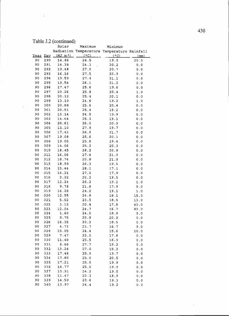
430
Table J.2 (continued)S o l a r Maximum Minimum
R a d i a t i o n Temp era ture Temperature R a i n f a l l Year Cay (MJ m' ) Lisn (°o __________ (mm)
90 290 1 4 . 8 6 2 4 . 5 1 9 . 9 2 5 . 090 291 1 4 .3 8 2 4 . 3 2 0 . 2 0 . 090 292 1 9 .4 8 2 7 . 0 2 0 . 7 0 . 090 293 1 6 . 1 6 2 7 . 5 2 0 . 9 0 . 090 294 1 9 . 5 9 2 7 . 4 2 1 . 1 0 . 090 295 1 9 .5 4 2 6 . 1 2 1 . 2 0 . 090 296 1 7 . 4 7 2 5 . 6 1 9 . 6 0 . 090 297 2 0 . 2 6 2 5 . 8 2 0 . 4 1 . 090 298 2 0 . 1 2 2 5 . 4 2 0 . 1 0 . 090 299 1 3 . 1 0 2 4 . 6 1 9 .2 1 . 090 300 2 0 . 8 8 2 5 . 6 2 0 . 4 0 . 090 301 2 0 . 5 1 2 5 . 4 1 9 .2 0 . 090 302 13 .14 2 4 . 5 1 9 . 9 0 . 090 303 1 4 .6 4 2 5 .3 1 9 . 1 0 . 090 304 2 0 . 6 1 2 6 . 0 2 0 . 9 0 . 090 305 1 5 .1 0 2 7 . 9 1 9 . 7 0 . 090 306 1 7 .4 3 2 6 . 6 2 1 . 7 0 . 090 307 1 9 .0 8 2 5 . 6 2 0 . 1 0 . 090 308 1 9 . 0 5 2 5 . 6 1 9 .4 0 . 090 309 1 4 .0 6 2 5 . 2 2 0 .3 0 . 090 310 18 .45 2 6 . 2 2 0 . 8 0 . 090 311 1 6 . 0 6 2 7 . 6 2 1 .3 0 . 090 312 18 .74 2 5 . 8 2 1 . 0 0 . 090 313 1 8 . 9 9 2 6 . 3 1 9 .5 0 . 090 314 1 5 .4 4 2 8 . 1 1 7 . 1 0 . 090 315 1 6 . 2 1 2 7 . 0 1 7 . 9 0 . 090 316 2 . 9 2 2 5 . 2 1 9 .5 0 . 090 317 1 2 .2 4 2 6 . 2 1 9 .2 1 . 090 318 9 . 7 8 2 1 . 6 1 7 .9 9 . 090 319 1 6 . 2 8 2 4 . 2 1 9 .1 1 . 090 320 1 2 .5 5 2 4 . 8 1 8 .1 1 5 . 090 321 5 . 5 2 2 3 . 5 18 .5 13 .090 322 3 .12 2 0 . 4 1 7 .8 43 .090 323 1 2 .0 4 2 4 . 7 16 .7 83 . 090 324 1 . 6 0 2 4 . 0 1 8 . 9 9 . 090 325 9 . 7 5 2 5 . 8 2 0 . 0 0 . 090 326 16 .35 3 0 . 3 18 .5 0 . 090 327 4 .73 2 3 . 7 1 6 . 7 9 .090 328 1 5 .0 5 2 4 . 4 1 5 .6 1 0 .090 329 7 . 4 7 2 2 . 5 1 7 .6 0 .090 330 1 1 .4 0 2 5 . 5 1 6 . 9 0 . 090 331 8 . 6 6 2 7 . 7 1 9 .2 0 . 090 332 13 .24 2 7 . 0 1 8 .3 0 . 090 333 1 7 . 4 6 2 5 . 9 1 9 . 7 0 . 090 334 1 7 . 8 0 2 5 . 0 2 0 . 5 0 . 090 335 1 7 .2 1 2 5 . 5 1 9 .9 0 . 090 336 14 .77 2 5 . 0 1 9 . 9 0 .090 337 1 3 . 9 1 2 4 . 2 1 9 . 5 0 .090 338 1 1 . 4 7 23 .3 1 8 . 9 0 .090 339 1 4 .5 0 23 .6 1 9 .3 0 .090 340 13 .97 24 .4 1 9 .2 0 .0
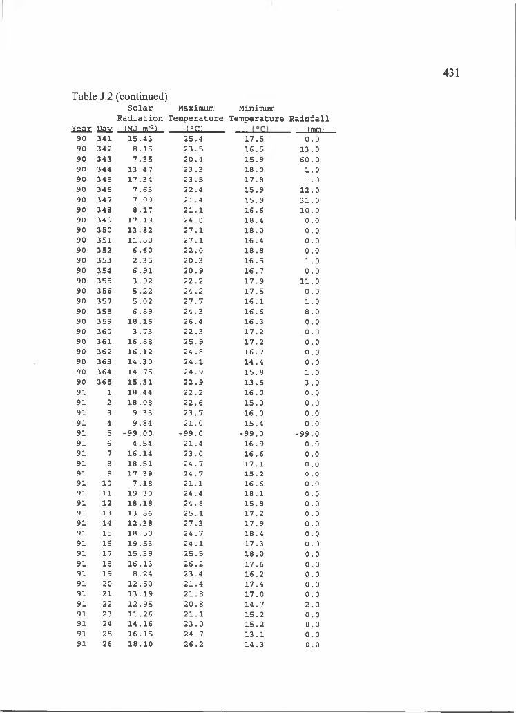
431
Y a a r C ay (MJ m~') LlCl _________ (mm)90 341 1 5 .4 3 2 5 . 4 1 7 . 5 0 . 090 342 8 . 1 5 2 3 . 5 1 6 . 5 1 3 . 090 343 7 . 3 5 2 0 . 4 1 5 . 9 6 0 . 090 344 1 3 . 4 7 2 3 . 3 1 8 . 0 1 . 090 345 1 7 . 3 4 2 3 . 5 1 7 . 8 1 . 090 346 7 . 6 3 2 2 . 4 1 5 . 9 1 2 . 090 347 7 . 0 9 2 1 . 4 1 5 . 9 3 1 . 090 348 8 . 1 7 2 1 . 1 1 6 . 6 1 0 . 090 349 1 7 . 1 9 2 4 . 0 1 8 . 4 0 . 090 350 1 3 . 8 2 2 7 . 1 1 8 . 0 0 . 090 351 1 1 . 8 0 2 7 . 1 1 6 . 4 0 . 090 352 6 . 6 0 2 2 . 0 1 8 . 8 0 . 090 353 2 . 3 5 2 0 . 3 1 6 . 5 1 . 090 354 6 . 9 1 2 0 . 9 1 6 . 7 0 . 090 355 3 . 9 2 2 2 . 2 1 7 . 9 1 1 . 090 356 5 . 2 2 2 4 . 2 1 7 . 5 0 . 090 357 5 . 0 2 2 7 . 7 1 6 . 1 1 . 090 358 6 . 8 9 2 4 . 3 1 6 . 6 8 . 090 359 1 8 . 1 6 2 6 . 4 1 6 .3 0 . 090 360 3 . 7 3 2 2 . 3 1 7 . 2 0 . 090 361 1 6 . 8 8 2 5 . 9 1 7 . 2 0 . 090 362 1 6 . 1 2 2 4 . 8 1 6 . 7 0 . 090 363 1 4 . 3 0 2 4 . 1 1 4 . 4 0 . 090 364 1 4 . 7 5 2 4 . 9 1 5 . 8 1 . 090 365 1 5 . 3 1 2 2 . 9 1 3 . 5 3 . 091 1 1 8 . 4 4 2 2 . 2 1 6 . 0 0 .091 2 1 8 . 0 8 2 2 . 6 1 5 . 0 0 . 091 3 9 . 3 3 2 3 . 7 1 6 . 0 0 .091 4 9 . 8 4 2 1 . 0 1 5 .4 0 .091 5 - 9 9 . 0 0 - 9 9 . 0 - 9 9 . 0 - 9 9 . 091 6 4 . 5 4 2 1 . 4 1 6 . 9 0 .091 7 1 6 . 1 4 2 3 . 0 1 6 . 6 0 .091 8 1 8 . 5 1 2 4 . 7 1 7 . 1 0 .091 9 1 7 . 3 9 2 4 . 7 1 5 . 2 0 .091 10 7 . 1 8 2 1 . 1 1 6 . 6 0 .091 11 1 9 . 3 0 2 4 . 4 1 8 . 1 0 .091 12 1 8 . 1 8 2 4 . 8 1 5 . 8 0 . 091 13 1 3 . 8 6 2 5 . 1 1 7 . 2 0 . 091 14 1 2 . 3 8 2 7 . 3 1 7 . 9 0 . 091 15 1 8 . 5 0 2 4 . 7 1 8 . 4 0 . 091 16 1 9 .5 3 2 4 . 1 1 7 .3 0 . 091 17 1 5 . 3 9 2 5 . 5 1 8 . 0 0 . 091 18 1 6 . 1 3 2 6 . 2 1 7 . 6 0 .091 19 8 . 2 4 2 3 . 4 1 6 . 2 0 . 091 20 1 2 . 5 0 2 1 . 4 1 7 . 4 0 . 091 21 1 3 . 1 9 2 1 . 8 1 7 . 0 0 . 091 22 1 2 . 9 5 2 0 . 8 1 4 . 7 2 . 091 23 1 1 . 2 6 2 1 . 1 1 5 . 2 0 . 091 24 1 4 . 1 6 2 3 . 0 1 5 . 2 0 .091 25 1 6 . 1 5 2 4 . 7 1 3 . 1 0 . 091 26 1 8 . 1 0 2 6 . 2 1 4 .3 0 .0
Table J.2 (continued)S o l a r Maximum Minimum
R a d i a t i o n T e m p e r a tu r e T e m p e ra tu r e R a i n f a l l
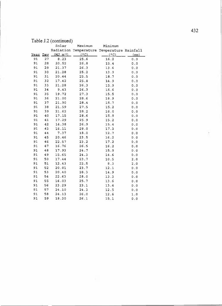
432
Table J.2 (continued)S o l a r Maximum Minimum
R a d i a t i o n Temperat ure Temperature R a i n f a l l Year Eay (MJ ___________________________________ (mm)
91 27 8 . 2 3 2 5 . G 1 6 . 2 0 . 091 28 2 0 . 5 2 2 6 . 8 1 5 .4 0 . 091 29 2 1 . 3 7 2 6 . 3 1 3 . 6 0 . 091 30 2 1 . 2 8 2 5 . 2 1 3 . 9 0 . 091 31 2 0 . 4 4 2 5 . 5 1 8 . 7 0 . 091 32 1 7 . 4 2 2 5 . 8 1 4 . 9 0 . 091 33 2 1 . 2 8 2 6 . 3 1 5 . 9 0 . 091 34 9 . 4 3 2 6 . 3 1 5 . 6 0 . 091 35 1 9 . 7 2 2 7 . 3 1 5 . 5 0 . 091 36 2 1 . 0 0 2 8 . 6 1 8 . 9 0 . 091 37 2 1 . 9 0 2 8 . 4 1 5 . 7 0 . 091 38 2 1 . 5 9 2 7 . 5 1 5 . 2 0 . 091 39 2 1 . 6 2 2 8 . 2 1 6 . 0 0 . 091 40 1 7 . 1 5 2 8 . 6 1 5 . 9 0 . 091 41 1 7 . 2 9 2 5 . 9 1 5 . 2 0 . 091 42 1 4 . 3 8 2 6 . 9 1 5 . 4 0 . 091 43 1 6 . 1 1 2 8 . 0 1 7 .3 0 . 091 44 7 . 3 7 1 8 . 0 1 2 . 7 0 . 091 45 2 0 . 4 6 2 3 . 5 1 6 . 2 0 . 091 46 2 2 . 5 7 2 3 . 2 1 7 . 2 0 . 091 47 1 6 . 7 6 2 6 . 5 1 6 . 2 0 . 091 48 1 7 . 9 3 2 4 . 7 1 5 . 9 0 . 091 49 1 5 . 6 5 2 4 . 3 1 4 . 6 0 . 091 50 1 7 . 4 4 2 3 . 7 1 0 . 5 2 . 091 51 1 2 . 4 3 2 2 . 5 8 .3 2 . 091 52 2 0 . 0 1 2 3 . 7 1 2 . 1 0 . 091 53 2 0 . 4 0 2 8 . 3 1 4 . 9 0 . 091 54 2 2 . 6 3 2 8 . 0 1 3 .3 0 . 091 55 1 6 .0 3 2 5 . 7 1 3 .6 0 . 091 56 2 3 . 2 9 2 3 . 1 1 3 . 4 0 . 091 57 2 4 . 1 0 2 4 . 3 1 2 . 5 0 . 091 58 2 4 . 1 3 2 6 . 0 1 2 . 6 1 . 091 59 1 8 . 3 0 2 6 . 1 1 5 . 1 0 . 0

REFERENCES
Anand, S.C. and J.H. Torrie. 1963. Heritability of yield and other traits andinterrelationships among traits in the Fj and F4 generations of three soybean crosses. Crop Sci. 3:508-511.
Ashour, N.I. and A.T. Thalooth. 1983. Effects of soil and foliar application ofnitrogen during pod development on the yield of soybean tGlvcine max (L.) Merr.) plants. Field Crops Res. 6:261-266.
AVRDC. 1991. 1990 Progress Report. Asian Vegetable Research and Development Center. Shanhua, Tainan.
Bartley, B.G. and C.R. Weber. 1952. Heritable and nonheritable relationships and variability of agronomic characters in successive generations of soybean crosses. Agron. J. 44:487-493.
Bhatnagar, G.S. and G.L. Jain. 1989. Effect of sowing dates and N fertilization on the phenology of maize varieties during winter. Intern. J. Trop. Ag. 7:237-242.
Board, J.E. and J.R. Settimi. 1988. Photoperiod requirements for flowering and flower production in soybean. Agron. J. 80:518-525.
Bonaparte, E.E.N.A. 1975. The effects of temperature, daylength, soil fertility andsoil moisture on leaf number and duration to tassel emergence in Zsa mavs L. Ann. Bot. 39:853-861.
Bonaparte, E.E.N.A. 1977. Diallel analysis of leaf number and duration to mid-silk in maize. Can. J. Genet. Cytol. 19:251-258.
Bonaparte, E.E.N.A. and R.I. Brawn. 1976. Effects of different environments on leaf number and duration to flowering in crops. Can. J. Plant Sci. 56:699-704.
Bonhomme, R., M. Derieux, and G.O. Edmeades. 1994. Flowering of diverse maize cuitivars in relation to temperature and photoperiod in multilocation field trials. Crop Sci. 34:156-164.
Boote, K.J., G.G. Wilkerson, and J.W. Jones. 1987. Modeling pod addition, shell growth, and seed growth, p. 17-26. In Simulation models for soybeans and other crops. Food and Fertilizer Technology Center, Tech. Bull. 106.
433
Breuer, C.M., R.B. Hunter, and L.W. Kannenberg. 1976. Effects of 10- and 20-hour photoperiod treatments at 20 and 30 C on rate of development of a singlecross maize tZea mavsl hybrid. Can. J. Plant Sci. 56:795-798.
Brewbaker, J.L. 1981. Maize improvement in relation to photoperiod sensitivity and incident solar radiation. Food and Fertilizer Technology Center, Tech. Bull, no. 59.
Brown, D.M. and L.J. Chapman. 1960. Soybean ecology II. Development-temperature-moisture relationships from field studies. Agron. J. 52:496-499.
Carter, M.W. and C.G. Poneleit. 1973. Black layer maturity and filling periodvariation among inbred lines of com (Zea mavs L.). Crop Sci. 13:436-439.
Chan, K.L., R.S. Lee, and F.S. Thseng. 1986. Genetic variation of soybean hybrid populations by natural selection in spring crop season at four locations II. Variations of heritabilities and correlations for certain agronomic characters in F2 generation. J. Agric. Res. China. 35:280-291.
Coligado, M.C. and D.M. Brown. 1975. Response of com tZea mavs L.) in the pretassel initiation period to temperature and photoperiod. Agric. Meteor. 14:357-367.
Constable, G.A. and LA. Rose. 1988. Variability of soybean phenology response to temperature, daylength and rate of change in daylength. Field Crops Res. 18:57-59.
Cooper, P.J.M. 1979. The association between altitude, environmental variables, maize growth and yields in Kenya. J. Agric. Sci. 93:635-649.
Cregan, P.B. and E.E. Hartwig. 1984. Characterization of flowering response to photoperiod in diverse soybean genotypes. Crop Sci. 24:659-662.
Dhillon, B.S., P.A. Gurrath, E. Zimmer, M. Wermke, W.G. Pollmer, and D. Klein. 1990. Analysis of diallel crosses of maize for variation and covariation in agronomic traits at silage and grain harvest. Maydica 35:297-302.
Djisbar, A. and F.P. Gardner. 1989. Heterosis for embryo size and source and sink components of maize. Crop Sci. 29:985-992.
434
Dombos, D.L., Jr., R.E. Mullen, and R.M. Shibles. 1989. Drought stress effectsduring seed fill on soybean seed germination and vigor. Crop Sci. 29:476-480.
du Pisani, A.L. 1987. The CERES-Maize model as a potential tool for drought assessment in South Africa. Water S. Africa 13:159-164.
Egli, D.B., J.E. Leggett, and W.G. Duncan. 1978. Influence of N stress on leaf senescence and N redistribution in soybeans. Agron. J. 70:43-47.
Egli, D.B., and I.E. Wardlaw. 1980. Temperature response of seed growth characteristics of soybeans. Agron. J. 72:560-564.
Ellis, R.H., R.J. Summerfield, G.O. Edmeades, and E.H. Roberts. 1992. Photoperiod, leaf number, and interval fi-om tassel initiation to emergence in diverse cultivars of maize. Crop Sci. 32:398-403.
Faluyi, M.A. 1990. Implications of selecting improved strains o f soybeans for dry- matter accumulation and grain yield. Euphytica. 50:197-201.
Flavelle, P. 1992. A quantitative measure of model validation and its potential use for regulatory purposes. Advances in Water Resources 15:5-13.
Frey, N.M. 1981. Dry matter accumulation in kernels of maize. Crop Sci. 21:118-122.
Furbringer, J.M. and R. Borchiellini. 1993. Technique of sensitivity analysis applied to an air infiltration multizone model. ASHRAE Trans. 99:683-691.
Gamble, E.E. 1962a. Gene effects in com (Zea mavs L.) I. Separation and relative importance of gene effects for yield. Can. J. Plant Sci. 42:339-348.
Gamble, E.E. 1962b. Gene effects in com tZea mavs L.) II. Relative importance of gene effects for plant height and certain component attributes of yield. Can. J. Plant Sci. 42:349-358.
Gamble, E.E. 1962c. Gene effects in com fZea mavs L.) III. Relative stability of the gene effects in different environments. Can. J. Plant Sci. 42:628-634.
Gomez, K.A. and A.A. Gomez. 1976. Statistical procedures for agricultural research, with emphasis on rice. International Rice Research Institute, Los Banos, Philippines.
435
Grant, R.F. 1989. Simulation of maize phenology. Agron. J. 81:451-457.
Grimm, S.S., J.W. Jones, K.J. Boote, and D.C. Herzog. 1994. Modeling theoccurrence of reproductive stages after flowering for four soybean cultivars. Agron. J. 86:31-38.
436
Hadley, P., E.H. Roberts, R.J. Summerfield, and F.R. Minchin. 1984. Effects of temperature and photoperiod on flowering in soya bean [Glvcine max (L.) Merrill]: a quantitative model. Ann. Bot. 53:669-681.
Hanway, J.J., and C.R. Weber. 1971. Dry matter accumulation in soybean (Glvcine max (L.) Merrill) plants as influenced by N, P, and K fertilization. Agron. J. 63:263-266.
Havens, P.L. and D.D. Fontaine. 1991. An introduction to sensitivity analysis. Aspects of Applied Biology 26:135-149.
Hesketh, J.D., D.L. Myhre, and C.R. Willey. 1973. Temperature control of timeintervals between vegetative and reproductive events in soybeans. Crop Sci. 13:250-254.
Hodges, T., D. Botner, C. Sakamoto, and J. Hay Haug. 1987. Using the CERES- Maize model to estimate production for the U.S. combelt. Agric. Forest Meteor. 40:293-303.
Howell, T.A., K.S. Copeland, A.D. Schneider, and D.A. Dusek. 1989. Sprinklerirrigation management for com - Southern Great Plain. Trans. ASAE 32:147- 160.
Hunt, P.G., T.A. Matheny, A.G. Wollum III, D.C. Reicosky, R.E. Sojka, and R.B. Campbell. 1983. Effect of irrigation and Rhizobium japonicum strain 110 upon yield and nitrogen accumulation of determinate soybean. Commun. Soil Sci. Plant Anal. 14:223-238.
Hunter, R.B. 1980. Increased leaf area (source) and yield of maize in short-season areas. Crop Sci. 20:571-574.
Hunter, R.B., L.A. Hunt, and L.W. Kannenberg. 1974. Photoperiod and temperature effects on com. Can. J. Plant Sci. 54:71-78.
Hunter, R.B., M. Tollenaar, and C.M. Breuer. 1977. Effects of photoperiod and temperature on vegetative and reproductive growth of a maize (Zea maysJ hybrid. Can. J. Plant Sci. 57:1127-1133.
Huxley, P.A., R.J. Summerfield, and A.P. Hughes. 1976. Growth and development of soyabean cv. TK5 as affected by tropical daylengths, day/night temperatures and nitrogen nutrition. Aim. Appl. Biol. 82:117-133.
Jain, R. 1991. The art of computer systems performance analysis: Techniques forexperimental design, measurement, simulation, and modeling. John Wiley and Sons, New York, NY.
Jha, P.B., A.S. Khehra, and S.A. Akhter. 1986. Stability analysis for grain development and yield in maize. Crop Improv. 13:16-19.
Johnson, H.W., H.A. Borthwick, and R.C. Leffel. 1960. Effects o f photoperiod and time of planting on rates of development of the soybean in various stages of the life cycle. Bot. Gazette 22:77-95.
Johnson, H.W., H.F. Robinson, and R.E. Comstock. 1955. Estimates of genetic and environmental variability in soybeans. Agron. J. 47:314-318.
437
Jones, C. A., and J. R. Kiniry. 1986. CERES-maize: a simulation model of maizegrowth and development. Texas A&M University Press, College Station, pp. 194.
Jones, C.A., J.T. Ritchie, J.R. Kiniry, and D.C. Godwin. 1986. Subroutine structure, p. 49-111. In C.A. Jones and J.R. Kiniry (ed.) CERES-Maize: A simulation model of maize growth and development. Texas A & M University Press, College Station, TX.
Jones, J.W., K.J. Boote, G. Hoogenboom, S.S. Jagtap, and G.G. Wilkerson. 1989.SOYGRO v5.42: Soybean crop growth simulation model user's guide. Florida Agricultural Experiment Station Journal No. 8304.
Jones, J.W., K.J. Boote, J.W. Mishoe, G.G. Wilkerson, and S.S. Jagtap. 1986. SOYGRO v5.3: Soybean crop growth and yield model IBSNAT version technical documentation, draft. Agricultural Engineering Department, University of Florida, Gainesville, FL.
Jones, R.J., B.G. Gengenbach, and V.B. Cardwell. 1981. Temperature effects on in vitro kernel development o f maize. Crop Sci. 21:761-766.
Jones, R.J., S. Ouattar, and R.K. Crookston. 1984. Thermal environment duringendosperm cell division and grain filling in maize: effects on kernel growth and development in vitro. Crop Sci. 24:133-137.
Kang, M.S., and D.P. Gorman. 1989. Genotype x environment interaction in maize. Agron, J. 81:662-664.
Kang, M.S., B.G. Harville, and D.P. Gorman. 1989. Contribution of weathervariables to genotype x environment interaction in soybean. Field Crops Res. 21:297-300.
Kaw, R.N., and P. Madhava Menon. 1978. Evaluation of soybean genotypes at Coimbatore. Madras Agric. J. 65:779-786.
Khadem, F.A., J.E. Specht, and J.H. Williams. 1985a. Soybean irrigation seriallytimed during stages R1 to R6.1. Agronomic responses. Agron. J. 77:291-298.
Khadem, F.A., J.E. Specht, and J.H. Williams. 1985b. Soybean irrigation serially timed during stages R1 to R6. II. Yield component responses. Agron. J. 77:299-304.
Kiniry, J.R., and J.T. Ritchie. 1985. Shade-sensitive interval of kernel number of maize. Agron. J. 77:711-715.
Kiniry, J.R., J.T. Ritchie, and R.L. Musser. 1983a. Dynamic nature of the photoperiod response in maize. Agron. J. 700-703.
Kiniry, J.R., J.T. Ritchie, R.L. Musser, E.P. Flint, and W.C. Iwig. 1983b. The photoperiod sensitive interval in maize. Agron. J. 75:687-690.
Konwar, B.K., and P. Talukdar. 1986. Stability analysis of yield and its components in soybean. Crop Improv. 13:172-175.
Kwon, S.H., and J.H. Torrie. 1964. Heritability o f and interrelationships among traits of two soybean populations. Crop Sci. 4:196-198.
LeClerg, E.L., W.H. Leonard, and A.G. Clark. 1962. Field plot technique. 2nd ed. Burgess Pub. Co., Minneapolis, MN.
438
Liu, W.T.H., D.M. Botner, and C.M. Sakamoto. 1989. Application of CERES-Maize model to yield prediction of a Brazilian maize hybrid. Agric. Forest Meteor. 45:299-312.
Major, D.J., D.R. Johnson, J.W. Tanner, and I.C. Anderson. 1975. Effects ofdaylength and temperature on soybean development. Crop Sci. 15:174-179.
Mann, J.D., and E.G. Jaworski. 1970. Comparison of stresses which may limit soybean yields. Crop Sci. 10:620-624.
Manrique, L.A. and T. Hodges. 1991. Development and growth of tropical maize at two elevations in Hawaii. Agron. J. 83:305-310.
McBlain, B.A., and R.L. Bernard. 1987. A new gene affecting the time of flowering and maturity in soybeans. J. Heredity 78:160-162.
McBlain, B.A., J.D. Hesketh, and R.L. Bernard. 1987. Genetic effects onreproductive phenology in soybean isolines differing in maturity genes. Can.J. Plant Sci. 67:105-115.
McClelland, T.B. 1928. Studies of the photoperiodism of some economic plants. J. Agric. Res. 37:603-628.
McIntosh, M.S. 1983. Analysis of combined experiments. Agron. J. 75:153-155.
Meckel, L., D.B. Egli, R.E. Phillips, D. Radcliffe, and J.E. Leggett. 1984. Effect of moisture stress on seed growth in soybeans. Agron. J. 76:647-650.
Milliken, G.A. and D.E. Johnson. 1989. Analysis of messy data. Volume 2; Nonreplicated experiments. Van Nostrand Reinhold, New York, NY.
Momen, N.N., R.E. Carlson, R.H. Shaw, and O. Aijmand. 1979. Moisture-stresseffects on the yield components of two soybean cuitivars. Agron. J. 71:86-90.
NeSmith, D.S., and J.T. Ritchie. 1992a. Effects of soil water-deficit during tasselemergence on development and yield component of maize fZea mavsl. Field Crops Res. 28:251-256.
NeSmith, D.S., and J.T. Ritchie. 1992b. Maize tZea mavs L.) response to a severe soil water-deficit during grain-filling. Field Crops Res. 29:23-35.
439

NeSmith, D.S., and J.T. Ritchie. 1992c. Short- and long-term responses of com to a pre-anthesis soil water deficit. Agron. J. 84:107-113.
Ottaviano, E., and A. Camussi. 1981. Phenotypic and genetic relationships between yield components in maize. Euphytica 30:601-609.
Parvez, A.Q. and P.P. Gardner. 1987. Daylength and sowing date responses of soybean lines with 'juvenile' trait. Crop Sci. 27:305-310.
Pathak, N.N., and D.P. Nema. 1988. Genotype-environment interaction for growth characteristics and yield in soybean. In Progress in ecology. Vol. 10. Advancement of crops and monitoring of environment (ed. G.P. Verma) pp.143-163. Today and Tomorrow's Printers and Publishers, New Delhi.
Peaslee, D.E., J.L. Ragland, and W.G. Dimcan. 1971. Grain filling period of com as influenced by phosphorus, potassium, and the time of planting. Agron. J. 63:561-563.
Perenzin, M,, F. Ferrari, and M. Motto. 1980. Heritabilities and relationships among grain-filling period, seed weight and quality in forty Italian varieties o f com tZea mavs L.l. Can J. Plant Sci. 60:1101-1107.
Peters, D.B., J.W. Pendleton, R.H. Hageman, and C.M. Brown. 1971. Effect of night air temperature on grain yield of com, wheat, and soybean. Agron. J. 63:809.
Pfeiffer, T.V., and D.B. Egli. 1988. Heritability o f seed filling period estimates in soybean. Crop Sci. 28:921-925.
Poneleit, C.G., and D.B. Egli. 1979. Kernel growth rate and duration in maize as affected by plant density and genotype. Crop Sci. 19:385-388.
Ragland, J.L., A.L. Hatfield, and G.R. Benoit. 1966. Photoperiod effects on the erar components of com, Zsa mavs L. Agron. J. 58:455-456.
Raper, C.B., Jr., and J.F. Thomas. 1978. Photoperiodic alteration of dry matter partitioning and seed yield in soybeans. Crop Sci. 18:654-656.
Raymer, P.L., and R.L. Bernard. 1988. Response of current midwestem soybean cultivars to late planting. Crop Sci. 28:761-764.
440

Ritchie, J.T., J.R. Kiniry, C.A. Jones, and P.T. Dyke. 1986. Model inputs, p. 37-48. In C.A. Jones and J.R. Kiniry (ed.) CERES-Maize: a simulation model of maize growth and development. Texas A«&M University Press, College Station, TX.
Ritchie, J.T., U. Singh, D.C. Godwin, and L.A. Hunt. 1989. A user's guide toCERES-Maize v2.10. International Fertilizer Development Center. Muscle Shoals, Alabama 35662, USA, 130 pp.
Rood, S.B., and D.J. Major. 1981. Diallel analysis of the photoperiodic response of maize. Crop Sci. 21:875-878.
Robins, J.S., and C.E. Domingo. 1956. Moisture deficits in relation to the growth and development o f dry beans. Agron. J. 48:67-70.
Russell, W.A. 1976. Genetic effects and genetic effects x year interactions at three gene loci in sublines of a maize inbred line. Can. J. Genet. Cytol. 18:23-33.
Russell, W.K., and C.W. Stuber. 1983a. Effects of photoperiod and temperatures on the duration of vegetative growth in maize. Crop Sci. 23:847-850.
Russell, W.K., and C.W. Stuber, 1983b. Inheritance of photosensitivity in maize.Crop Sci. 23:935-939.
Russell, W.K., and C.W. Stuber. 1985. Genotype x photoperiod and genotype x temperature interactions for maturity in maize. Crop Sci. 25:152-158.
Saindon, G., H.D. Voldeng, W.D. Beversdorf, and R.I. Buzzell. 1989a. Genetic control of long daylength response in soybean. Crop Sci. 29:1436-1439.
Saindon, G., W.D. Beversdorf, and H.D. Voldeng. 1989b. Adjustment o f the soybean phenology using the E4 locus. Crop Sci. 29:1361-1365.
Saindon, G., H.D. Voldeng, and W.D. Beversdorf. 1990. Adjusting the phenology of determinate soybean segregants grown at high latitude. Crop Sci. 30:516-521.
Saito, M. 1961. Studies on the influence of low temperature on soybean plants. I.Effects of day or night temperature on the growth and ripening of plants. Res. Bull. Hokkaido National Agric. Exp. Sta. 76:9-14.
Schoper, J.B., R.R. Johnson, and R.J. Lambert. 1982. Maize yield response to increased assimilate supply. Crop Sci. 22:1184-1189.
441

Schutz, W.M., and R.L. Bernard. 1967. Genotype x environment interactions in the regional testing of soybean strains. Crop Sci. 7:125-130.
Schweitzer, L.E., and J.E. Harper. 1985. Effect of hastened flowering on seed yield and dry matter partitioning in diverse soybean genotypes. Crop Sci. 25:995- 998.
Seddigh, M., and G.D. Jolliff. 1984. Effects of night temperature on dry matterpartitioning and seed growth of indeterminate field-grown soybean. Crop Sci. 24:704-710.
Shaw, R.H., and H.C.S. Thom. 1951. On the phenology of field com, the vegetative period. Agron. J. 43:9-15.
Singh, V.K., B.D. Singh, J.P. Shahi, and R.P. Singh. 1989. Estimates o f genetic variances in a population of maize. Crop Improv. 16:29-33.
Sionit, V., and P. J. Kramer. 1977. Effect of water stress during different stages of growth o f soybean. Agron. J. 69:274-278.
Smith, J.R., and R.L. Nelson. 1987. Predicting yield from early generation estimates of reproductive growth periods in soybean. Crop Sci. 27:471-474.
Statistical Engineering Laboratory. 1957. Fractional factorial experiment designs for factors at two levels. National Bureau of Standards Applied Mathematics Series 48. U.S. Gov. Print. Office, Washington, D.C.
Stuber, C.W., R.H. Moll, and W.D. Hanson. 1966. Genetic variances andinterrelationships of six traits in a hybrid population of Zea mavs L. Crop Sci. 6:455-458.
Summerfield, R.J. and E.H. Roberts. 1985. Glvcine max. p. 100-117. In A.H. Halevy (ed.) CRC handbook of flowering. Vol. 1. CRC Press, Boca Raton, FL.
Swaney, D. P., J. W. Jones, W. G. Boggess, G. G. Wilkerson, J. W. Mishoe. 1983.Real-time irrigation decision analysis using simulation. Trans. ASAE 26: 562- 568.
Thomas, J.F., and C.B. Raper, Jr. 1976. Photoperiodic control of seed filling for soybeans. Crop Sci. 16:667-672.
442

Thomas, J.F., and C.B. Raper, Jr. 1983. Photoperiodic and temperature regulation of floral initiation and anthesis in soya bean. Ann. Bot. 51:481-489.
van Schaik, P.H., and A.H. Probst. 1958. Effects of some environmental factors on flower production and reproductive efficiency in soybeans. Agron. J. 50:192- 197.
Warrington, I.J. and E.T. Kanemasu. 1983a. Com growth response to temperature and photoperiod. I. Seedling emergence, tassel initiation, and anthesis. Agron J. 75:749-754.
Warrington, I.J. and E.T. Kanemasu. 1983b. Com growth response to temperature and photoperiod. II. Leaf-initiation and leaf-appearance rates. Agron. J. 75:755-761.
Warrington, I.J. and E.T. Kanemasu. 1983c. Com growth response to temperature and photoperiod. III. Leaf number. Agron. J. 75:762-766.
Weber, C.R. 1966. Nodulating and nonnodulating soybean isolines: I. Agronomic and chemical attributes. Agron. J. 58:43-46.
Westgate, M.E., J.R. Schussler, D.C. Reicosky, and M.L. Brenner. 1989. Effect of water deficits on seed development in soybean. II. Conservation of seed growth rate. Plant Physiol. 91:980-985.
Wien, H.C., E.J. Littleton, and A. Ayanaba. 1979. Drought stress of cowpea and soybean under tropical conditions. In Stress physiology in crop plants, pp. 283-301. H. Mussel and R.C. Staples (ed.) John Wiley and Sons, Inc., New York.
Wilkerson, G. G., J. W. Jones, K. J. Boote, K. T. Ingram, and J. W. Mishoe. 1983. Modeling soybean growth for crop management. Trans. ASAE 26: 63-73.
Willmott, C.J. 1981. On the validation of models. Physical Geography 2:184-194.
Willmott, C.J. 1982. Some comments on the evaluation o f model performance. American Meteorological Society 63:1309-1313.
443