determinants of gross domestic savings in uganda
TRANSCRIPT
MAKERERE UNIVERSITY
COLLEGE OF BUSINESS AND MANAGEMENT SCIENCES
DETERMINANTS OF GROSS DOMESTIC SAVINGS IN UGANDA
BY
NAGAWA VIVIAN
2016/HD06/1213U
A DISSERTATION SUBMITTED TO THE DIRECTORATE OF RESEARCH AND
GRADUATE TRAINING IN PARTIAL FULFILLMENT OF THE
REQUIREMENTS FOR THE AWARD OF THE DEGREE
OF MASTER OF ARTS IN ECONOMICS OF
MAKERERE UNIVERSITY
DECEMBER 2018

i
DECLARATION
I, NAGAWA VIVIAN hereby declare that this dissertation entitled ―Determinants of Gross
Domestic Savings in Uganda” is my original work and has not been presented by anyone - for
the award of a degree in any other university or institution of higher learning.

ii
APPROVAL
This dissertation is submitted for the award of the degree of Master of Arts in Economics of
Makerere University with our approval as University Academic Supervisors.

iii
DEDICATION
This dissertation is dedicated to my family and friends for loving, caring and supporting me
during this course.

iv
ACKNOWLEDGEMENT
Praise be to the Almighty GOD for the gift of life, determination, knowledge and understanding
he has given to me while pursuing this course. I also wish to extend my sincere appreciation to
the following people who made this dissertation possible.
This dissertation would not be possible without the significant contributions of my supervisors.
Therefore, I would like to express my sincere appreciation to my dedicated supervisors,
Associate Professor. Edward Bbaale and Dr. Francis Wasswa, for their invaluable advice,
guidance and suggestions which made my dissertation a success.
I would also like to appreciate all my lecturers for their guidance during the first year of
theoretical foundation of this degree. In this regard, special thanks goes to Dr. Mukisa Ibrahim
for the fatherly love and care accorded to me during this course, may God reward you
abundantly.
I am also grateful to my family members especially my elder sister, Nakigudde Jovious; grand
mum, Ms Immaculate Namakula Nalongo; mother, Ms Nice Diana Kalungi and little sister,
Natukunda Bonny who have been my support system during the study period and dissertation
writing period.
My sincere appreciation also goes to Dr. Ibrahim Kasirye; the Principal Research Fellow at the
Economic Policy Research Centre (EPRC) for all the support and guidance given to me before
and during my course.
I extend my sincere gratitude to my classmates; Naluwooza Patricia, Sunday Nathan, Kahunde
Reheme, Atwine Blessing, Atugonza Rashid, Musiimenta Hannington, Prowd Roosevelt and
Ahebwa Devis for their significant contributions and encouragements during the whole period of
study. Thank you guys for making the course and the dissertation a success. Special thanks goes
to my friends; Titus Mataki, Pamela Eunice and Kasule Samuel for creating time in their busy

v
schedules to read through and correct my dissertation and to Madam Amiinah Balunywa for all
that she did for me during this period. God bless you all always.
I also want to acknowledge the African Economic Research Consortium (AERC) for their
sponsorship to the Joint Facility for Electives (JFE).
However, I would like to disassociate all the people and institutions acknowledged above from
any errors in this piece of work. I am solely responsible for all the mistakes you will find in this
paper.

vi
TABLE OF CONTENTS
DECLARATION............................................................................................................................. i
APPROVAL ................................................................................................................................... ii
DEDICATION.............................................................................................................................. iii
ACKNOWLEDGEMENT ............................................................................................................ iv
LIST OF FIGURES ...................................................................................................................... ix
LIST OF TABLES ......................................................................................................................... x
LIST OF ACRONYMS ................................................................................................................ xi
ABSTRACT .................................................................................................................................. xii
CHAPTER ONE ............................................................................................................................ 1
INTRODUCTION.......................................................................................................................... 1
1.0 Introduction ................................................................................................................................ 1
1.1 Background of the Study ........................................................................................................... 1
1.2 Trend of savings in Uganda ....................................................................................................... 4
1.3 Statement of the Problem ........................................................................................................... 6
1.4 Objectives of the Study .............................................................................................................. 7
1.5 Significance of the Study ........................................................................................................... 7
1.6 Scope .......................................................................................................................................... 8
1.7 Organisation of the Thesis ......................................................................................................... 8
CHAPTER TWO ........................................................................................................................... 9
LITERATURE REVIEW ............................................................................................................. 9
2.0 Introduction ................................................................................................................................ 9
2.1 Theoretical Literature ................................................................................................................. 9
2.1.1 Absolute Income Hypothesis (Keynesian Theory) ................................................................. 9
2.1.2 Relative Income Hypothesis (RIH) ....................................................................................... 10
2.1.3 Permanent Income Hypothesis (PIH) ................................................................................... 11

vii
2.1.4 Life Cycle Hypothesis (LCH) ............................................................................................... 11
2.1.5 The McKinnon-Shaw Hypothesis ......................................................................................... 12
2.2 Empirical Literature ................................................................................................................. 13
2.3 Summary and Research Gap .................................................................................................... 18
CHAPTER THREE ..................................................................................................................... 19
METHODOLOGY ...................................................................................................................... 19
3.0 Introduction .............................................................................................................................. 19
3.1 Theoretical Model .................................................................................................................... 19
3.2 Model Specification ................................................................................................................. 22
3.3 Hypotheses ............................................................................................................................... 23
3.4 Estimation Model ..................................................................................................................... 23
3.5 Variable Description, Data type and source ............................................................................ 24
3.6 Data analysis and Estimation Techniques/ Procedures ............................................................ 24
3.6.1 Graphical analysis of the data and Unit root tests ................................................................. 24
3.6.1.1 Augmented Dickey Fuller .................................................................................................. 25
3.6.1.2 Phillips-Perron ................................................................................................................... 26
3.6.2 Cointegration Test ................................................................................................................. 27
3.6.3 Diagnostic Tests .................................................................................................................... 30
3.6.3.1 Ramsey Regression Equation Specification Error Test (RESET) test: ............................. 30
3.6.3.2 The Jarque-Bera Test ......................................................................................................... 31
3.6.3.3 The Breusch–Godfrey serial correlation LM test .............................................................. 31
3.6.3.4 Breusch-Pagan test ............................................................................................................. 32
3.6.3.5 Variance inflation factor (VIF) .......................................................................................... 32
3.6.3.6 The CUSUM and CUSUMSQ test .................................................................................... 33
viii
CHAPTER FOUR ........................................................................................................................ 34
PRESENTATION, INTERPRETATION AND DISCUSSION OF RESULTS ..................... 34
4.0 Introduction .............................................................................................................................. 34
4.1 Data Description ...................................................................................................................... 34
4.2 Correlation Matrix of Variables ............................................................................................... 36
4.3 Time series properties of the data ............................................................................................ 37
4.4 Estimation Results ................................................................................................................... 39
4.4.1 Autoregressive Distributed Lag Model (ARDL) to Cointegration ....................................... 40
4.4.2 Estimation of the ARDL model ............................................................................................ 44
4.5 Discussion of Results ............................................................................................................... 46
CHAPTER FIVE ......................................................................................................................... 50
SUMMARY, CONCLUSIONS AND POLICY IMPLICATIONS ......................................... 50
5.0 Introduction .............................................................................................................................. 50
5.1 Summary of the Key Findings ................................................................................................. 50
5.2 Conclusions .............................................................................................................................. 51
5.3 Policy Implications and Recommendations ............................................................................. 52
5.4 Limitations of the Study........................................................................................................... 53
5.5 Areas for further Study ............................................................................................................ 53
REFERENCES ............................................................................................................................. 55
APPENDICES .............................................................................................................................. 59
APPENDIX 1: UGANDA‘S DEBT PERCAPITA _ 2007-2016 .................................................. 59
APPENDIX 2: Derivation of the Theoretical Framework ............................................................. 60
APPENDIX 3: Variable Description and Expected Sign .............................................................. 67
APPENDIX 4: Graphical plots of the variables ............................................................................ 69
APPENDIX 5: Variance inflation factors results (VIF) ................................................................ 71
APPENDIX 6: CUSUM and CUSUMsq control charts ................................................................ 72

ix
LIST OF FIGURES
Figure 1.1: Uganda‘s Gross Domestic Savings Rate: 1960-2017.................................................... 5

x
LIST OF TABLES
Table 4. 1: Descriptive Statistics (percentages) ............................................................................. 34
Table 4. 2: Correlation Matrix ....................................................................................................... 36
Table 4. 3: ADF and PP Unit Root Tests for Stationarity: Levels and First difference ................ 38
Table 4. 4: Results of bounds test using F-statistic (U=upper, L=lower) ...................................... 40
Table 4. 5: Breusch-Godfrey Serial Correlation Test Results ....................................................... 41
Table 4. 6: Breusch-Pagan / Cook-Weisberg test for Heteroscedasticity Results ......................... 41
Table 4. 7: Ramsey RESET Test for model specification Results ................................................ 42
Table 4. 8: Jarque-Bera test for normality Results ........................................................................ 42
Table 4. 9: Long run coefficients and short run dynamics for ARDL (1 1 1 0 3 0 0) ................... 44
Table 4. 10: Short run dynamics .................................................................................................... 46

xi
LIST OF ACRONYMS
ADF : Augmented Dickey Fuller
AIC : Alkaike Information Criterion
ARDL : Autoregressive Distributed Lag Model
BG : Breusch Godfrey
BP : Breusch-Pagan
CAB : Current Account Balance
DIR : Deposit Interest Rate
DSA : Debt Sustainability Analysis
FDI : Foreign Domestic Investment
GDP : Gross Domestic Product
GDS : Gross Domestic Savings
GMM : Generalized Method of Moments
GNE : Gross National Expenditure
GNP : Gross National Product
GOU : Government of Uganda
HIPC : Highly Indebted Poor Country
M2 : Broad money
PP : Phillips Peron
RESET : Regression Equation Specification Error Test
SBIC : Schwarz Bayesian Information Criterion
URN : Uganda Radio Network
VECM : Vector Error Correction Mechanism
WDI : World Bank Development Indicators

xii
ABSTRACT
In Uganda‘s development aspiration ―VISION 2040‖, Uganda aspires to transform its society
from a peasant to a modern and prosperous middle-income country by 2040, with per capita
income of USD 9, 567. It is a commitment that to achieve the vision, savings as a percentage of
GDP should be over 35 percent. Notwithstanding such a high commitment, GDS as a percentage
of GDP has remained below the desired target, standing at 16.5 percent in 2017. The objective of
this study was to empirically establish the determinants of gross domestic savings (GDS) in
Uganda. The study was guided by the lifecycle/permanent income hypothesis theoretical
framework. The study used time series annual data from World Development Indicators for the
period 1980 to 2017; and used Augmented Dickey Fuller and Phillips Perron tests to check time
series properties of the variables. The unit root tests revealed that variables were both integrated
of order zero and one. Accordingly, to test for both the long-run relationship and short run
dynamics of the model, ARDL bounds test was adopted. The empirical results suggested that in
the long run, Gross Domestic Product growth rate (GDPg), Broad money (M2) and Foreign
Domestic Investments (FDI) have a positive impact on savings, while Current Account Balance
(CAB) and Gross National Expenditure (GNE) have a negative effect on savings. The study also
revealed that deposit interest rate was not a statistically significant determinant of GDS in the
long run. The short run results on the other hand showed that all except CAB and GDPg have a
positive and statistically significant impact on GDS. The key policy messages of this study are
twofold that is: First, there is need for export promotion and import substitution strategies to
improve on current account balance and hence savings through their impact on GDP. Second,
there is need to ensure a stable economic environment to attract more Foreign Direct
Investments.

1
CHAPTER ONE
INTRODUCTION
1.0 Introduction
This chapter introduces the context of the study, problem statement, study objectives and the
scope of the study. In addition, it provides definitions of key terms used in this study.
1.1 Background of the Study
There is greater consensus that the accumulation of savings is one of the most important
determinants of sustainable economic growth (Nwachukwu, 2012, Perez & Muturi, 2015). A
country‘s domestic savings— defined as the total sum of savings by households, businesses and
government in a given economy—plays a very vital role in attaining rapid and sustainable
economic growth. Higher rate of savings increases funds available for investment and hence
capital formation. This in turn leads to an increase in production and employment leading to
economic growth and development. Implying that low savings rate is a hindrance to substantial
economic growth. This implies that policies to stimulate economic growth should be geared
towards increasing the level of saving (Tesha, 2013).
The positive role of savings in fostering growth is well studied in the economic literature. Harrod
Domar model (1939) suggests that the rate of growth of an economy is positively related to the
economy‘s savings ratio. For an economy to grow, it should save a percentage of its Gross
National Product (GNP)1 to facilitate capital formation. A standard neo-classical model of
economic growth developed by Robert Solow in 1956 suggests that higher savings precedes
1Gross national product (GNP) is an estimate of total value of all the final products and services produced in a given
period by the means of production owned by a country's residents.

2
economic growth. In other words, an increase in savings rate leads to an increase in investment,
which leads to higher economic growth. However, this only happens in the short run. In the long
run, the equilibrium rate of growth is due to technological progress and growth of the labour
force (Solow, 1956).
Endogenous Growth Theory as suggested by Romer (1986) and Lucas (1988), asserts that high
savings and investment rates are important due to their strong and positive association with the
GDP growth rate. Consistent with theoretical model results, there is a broad consensus in the
empirical literature that low domestic savings is one of the major factors that hinder the
attainment of higher and sustainable economic growth (Perez & Muturi, 2015; Adelakun, 2015;
Manamba, 2014; Nwachukwu, 2012; Adewuyi et al, 2007; Tesha, 2013; Keho, 2011). For
instance, East Asian economies such as China, India, Indonesia, Malaysia, Singapore, South
Korea, and Thailand, which witnessed rapid economic growth rates, are also characterized by
high saving rates (Amaresh and Suresh, 2014).
The low rates of economic growth in many Sub-Saharan African countries can to a large extent
be attributed to the low levels of domestic savings (Tesha, 2013). This makes them depend
highly on foreign assistance in form of loans and aid which makes them vulnerable to external
shocks since the foreign assistance is never certain and hence distorting the budgeting and
planning process (Imoughele, 2014). To minimize vulnerability to external political and
economic shocks, a country like Uganda should endeavour to finance its investment needs using
internally generated funds (Manamba, 2014).

3
The nexus between savings and economic growth is particularly important for a small
developing country like Uganda - whose development agenda as enshrined in the ―VISION
2040‖, aspires to transform Ugandan society from a peasant to a modern and prosperous middle-
income country by 2040, with per capita income of USD 9, 567 (GOU, 2013). To attain the
vision, the country needs to generate sufficient resources to fund the key investment needs. There
are many ways through which Uganda can raise resources for her investment needs, among
which are but not limited to, taxation, borrowing and domestic saving. However, borrowing from
abroad as a source of investment capital has its own short and long-term effects including - debt
accumulation which can affect macroeconomic stability.
The Ugandan government has for the past years, been borrowing to improve the quality of
infrastructure mainly electricity and transportation in order to lay a firm foundation for future
growth (IMF, 2016) and to help in the achievement of the Vision 2040. However, although
borrowing to finance productive sectors of the economy is known to be good, it has led to an
increase in Uganda‘s debt portfolio from 6 billion dollars in 2012 to 10 billion dollars in 2016/17
(MoFPED, 2017). The current debt portfolio represents 34% of Gross Domestic Product and is
8.1 percentage points higher than that of 2012/13 financial year (MoFPED). Although according
to the DSA indicators the debt is still sustainable, it poses a challenge of mortgaging present and
future generation to an imposed obligation to pay back the loans. That is, the per capita debt in
Uganda stood at $258 in 2016 up from $108 in 2007 (Uganda Debt Network, 2017) as can be
seen in Appendix 1.
The increased debt has also increased the risk of failure by Government to service these loans,
which has made Uganda vulnerable to defaulting (IMF, 2017) as was the case twenty years ago
when Uganda‘s debt reached unsustainable levels. Fortunately Uganda benefited from debt

4
reliefs under the Highly Indebted Poor Country (HIPC) Initiative in 1998 and later on in 2000
under the Enhanced HIPC which saw her external debt levels reduce to approximately Shs 14
billion. (UDN, 2017). While currently Uganda‘s debt level is still sustainable and not expected to
affect growth, much effort should be geared towards increasing domestic savings in order to
avoid replay of history‖ (Kasekende, 2017). High debt levels (albeit still sustainable) coupled
with low tax-GDP ratio that is tax revenue as a percentage of GDP stood at 14.05% in FY
2016/17 (URA, 2018) leave gross domestic savings as the only feasible option to facilitate
Uganda‘s investment needs and achieve the VISION 2040.
Indeed, VISION 2040 acknowledges that one of the major constraints to Uganda‘s development
is the low level of savings, which has denied the country cheap investment capital. To achieve
the vision, savings as a percentage of GDP should be over 35 percent (GOU, 2013). However,
Uganda‘s savings rate as a percentage of GDP stood at 16.5 percent in 2017 (WDI, 2018) which
is too low to foster sustainable economic growth and thus achieve the vision.
1.2 Trend of savings in Uganda
Uganda is one of the Sub Saharan Africa countries characterized by low savings rates. Its GDS
as a percentage of GDP has been fluctuating for the past 30 or so years. The highest recorded
18.89 percent in 1964. Four years later, it declined to 14.41 percent, which bounced back to
17.23 percent in 1970 due to increased private and official transfers from abroad (Rujumba,
1999) which later declined to 5.7 percent in 1975.

5
By 1980, GDS had plummeted to -0.43 percent mainly on the account of civil war declared by
then president of Uganda Iddi Amin that resulted into expulsion of Asians from Uganda which
affected Uganda‘s macroeconomic stability. By the end of the civil war in 1987, Uganda‘s GDS
as a percentage of GDP had declined further to -0.08 percent.
Figure 1.1: Uganda’s Gross Domestic Savings Rate: 1960-2017
Source: Author’s computation from World Development Indicators database for 2018
The macroeconomic stabilization efforts that started in early 1990s, which included Economic
Recovery Program (ERP) and Structural Adjustment Programs which started with currency
reform, devaluations, liberalization of domestic prices, and eventually floating exchange rate
regime by 1993 boosted GDS and by 1994 it had recovered to 4.3 percent. From 2006 to 2008,
GDS as a percentage of GDP increased from 8.04 percent to 15.3 percent. This was mainly
driven by increased private and official transfers from abroad. By the end of 2017, it stood at
16.5 percent - which is below average of 17.2 percent for the sub Saharan Africa (Trading
economies, 2017) and lower than that of neighboring countries - Tanzania (21.5 percent) and
Congo Rep (28.06 percent).
-5
0
5
10
15
20
19
60
19
62
19
64
19
66
19
68
19
70
19
72
19
74
19
76
19
78
19
80
19
82
19
84
19
86
19
88
19
90
19
92
19
94
19
96
19
98
20
00
20
02
20
04
20
06
20
08
20
10
20
12
20
14
20
16
Savi
ngs
rat
e
Years
Uganda's GDS 1960-2017
6
There are several interventions by the government of Uganda to increase domestic savings.
These include; appropriate monetary policies to ensure positive interest rates on deposits;
policies to increase domestic taxes (e.g., broadening the tax base; increasing efficiency of
collection; and ensuring equity of taxation). However, these policy reforms have yielded minimal
results. Despite the notable improvement in the gross domestic savings shown by the upward
trend from 1992 onwards, savings still remain too low to support the country‘s development
agenda (GOU, 2017).
Therefore, there is need to investigate the determinants of GDS in Uganda. Evidence based
findings from such analysis can be useful in providing guidance and informing policy makers on
appropriate interventions needed to boost the country‘s levels of internally generated resources.
1.3 Statement of the Problem
In Uganda‘s development aspiration ―VISION 2040‖, Uganda aspires to transform its society
from a peasant to a modern and prosperous middle-income country by 2040, with per capita
income of USD 9, 567 (GOU, 2013). In order to fund investments large enough to attain
sustainable economic growth and achieve the Vision, the country needs a change in individuals‘
consumption, incomes and savings behavior as well as increased generation of government
resources. Savings is one of the financing mechanisms that can drive us to the Vision.
It is a commitment that to achieve the vision, savings as a percentage of GDP should be over 35
percent (GOU, 2013). Notwithstanding such a high commitment, current trends show that GDS
as a percentage of GDP has remained below the desired target by 19 points, standing at 16.5
percent in 2017 (World Bank, 2018). Low savings coupled with huge external and domestic
debt, low taxes as a percentage of GDP plus high infrastructural developments may not spur the

7
required growth levels for the country to achieve the Vision 2040. Therefore there is need to
study the determinants of GDS in Uganda since it is the cheapest source of investment capital for
the investment needs of Uganda.
1.4 Objectives of the Study
General objective of the Study
The main objective of the study is to investigate the determinants of gross domestic savings in
Uganda. Specifically, the study aims to investigate the effect of
Gross domestic product growth rate on gross domestic savings,
Monetary policy (Deposit interest rate and broad money) on gross domestic savings,
The external sector (current account balance) on gross domestic savings ratio.
1.5 Significance of the Study
Limited empirical work has been done on the determinants of gross domestic savings for the case
of Uganda. Most of the studies on Savings have concentrated on determinants of household
savings in Uganda (Obwona and Ddumba 1998; Namanya 2011). Other studies like that of
Mpiira et al. (2014) looked at determinants of net savings deposits held in saving and credit
cooperatives in Uganda while Gina et al. (2012) studied the determinants of Saving among Low-
Income Individuals in Rural Uganda. Studies that concentrated on Determinants of Gross
Domestic Savings in Uganda like that of Kaberuka and Namubiru (2014) and that of Keino and
Kairuki (2016) did not include variables like Current Account Balance, Foreign Direct
Investment and Gross National Expenditure which may be important determinants of the
behavior of gross domestic savings in Uganda.

8
This study therefore adds to the available literature in Uganda and the overall body of knowledge
by looking at the determinants of Gross Domestic Savings in Uganda complementing on the
previous works done by adding three variables that may be good in explaining savings that is;
Foreign Direct Investment (FDI), Current Account Balance (CAB) and Absorption / Gross
National Expenditure (GNE). The study also uses a longer and more recent time series that is
1980 to 2017 in addition to using modern time series procedures in analysis.
In addition, the findings of this study will provide useful policy insights to the policy makers in
Uganda in order to address the problem of low gross domestic savings in Uganda and reduce
reliance on external funds for investment.
1.6 Scope
The study will focus on the determinants of gross domestic savings in Uganda over the period
1980-2017. The choice of the time scope was due to availability and consistency of data.
1.7 Organisation of the Thesis
The thesis comprises of five chapters. Chapter one is the introduction which contains the
Background to the study, problem statement, objective, hypotheses, significance and the scope of
the study. Chapter two presents both the theoretical and empirical literature review. Chapter
three presents the methodology of the study which includes the theoretical framework, empirical
model specification, estimation procedures and data used in the study. Chapter four provides the
study findings and discussions. Finally, chapter five presents the summary, conclusion and
policy recommendations of the study.
9
CHAPTER TWO
LITERATURE REVIEW
2.0 Introduction
This chapter presents literature review related to the subject under study. The chapter is
organized into two main sections. Section 2.1 presents the review of theoretical literature of
savings. Section 2.2 presents a review of empirical studies on determinants of savings. The
chapter concludes by highlighting the contribution of this study to the existing body of
knowledge, particularly in the Ugandan context.
2.1 Theoretical Literature
Savings and consumption are normally considered together in most theories of savings. This is
because if a decision to consume is made, it implies another decision of not saving what is
consumed (Makone, 2016). Households do not spend their entire disposable incomes on current
consumption, they save part of it for future consumption. This also applies to the economy as
part of the national income is saved to form public savings- the difference between how much
money the government collects in tax revenue (T) minus its spending (G). There are five major
theories that explain the savings and consumption behaviour of economic agents. These are
explained in proceeding sub-sections.
2.1.1 Absolute Income Hypothesis (Keynesian Theory)
The Absolute Income Hypothesis (AIH) proposed by Keynes in 1936 establish the relationship
between income, consumption and savings. According to Keynes household consumption and
savings are an increasing function of absolute/ current disposable income. Keynes postulates that
other things being constant, consumption will increase at a decreasing rate as the income
increases. This implies that as disposable income rise, part of it is saved at an increasing rate.

10
Under this theory, the marginal propensity to consume (MPC) is a parameter bounded between
zero and one while the marginal propensity to save is a positive constant less than unity, so that
higher income leads to higher savings. This implies that MPC declines with increase in income
while MPS increases as income increases. The AIH theory implies that ceteris paribus, rich
people save more than poor people.
2.1.2 Relative Income Hypothesis (RIH)
The Relative Income Hypothesis (RIH) was developed by James Duesenberry in 1949.
According to this theory, consumption does not depend on absolute income like Keynes asserted,
but rather on relative income - current income of the individual relative to income of others in
society with whom the consumer feels he is competing with which is the reference group. It is
the relative position in the income distribution among individual households that influences the
consumption decisions of the individuals (Duesenberry, 1949). A household‘s consumption is
determined by the income and the expenditure pattern of their neighbors. There is a tendency of
the individual to imitate the consumption standards of their neighbors- the so called ‗keeping up
with the joneses‘ effect implying that such individuals tend to consume more and save less
(Duesenberry, 1949).
The RIH suggests that an upward change in income of a household may not necessarily lead to a
similar upward change in consumption level than the one already achieved. This implies that the
saving rate of such a household will increase due to increase in income. In such a case, the MPS
of an individual household would be higher if his relative position in the income distribution is
higher. A decline in income on the other hand results into a less than proportionate decline in
consumption. This is because households repel changing their consumption patterns to

11
accommodate the decline. This implies that lower income households allocate their income on
consumption and higher income households save most of their income (Duesenberry, 1949).
2.1.3 Permanent Income Hypothesis (PIH)
Permanent Income Hypothesis (PIH) was developed by Milton Friedman in 1957. According to
this theory, consumption depends neither on absolute income nor on relative income but on
permanent income based on expected future income. This hypothesis divides income and
consumption into two major components; transitory and permanent components. Permanent
income is the mean income determined by the expected income to be earned over a long period.
Transitory income on the other hand is the unexpected increase or reduction in income
(Friedman, 1957). Transitory consumption is unanticipated consumption. Friedman‘s basic
assumption is that permanent consumption depends on permanent income and hence there is a
fairly constant average propensity to consume. An economic agent‘s consumption at any time t is
related with their total lifetime income/ permanent income. This means that individual
consumption behaviour does not change due to changes in the transitory income but due to
changes in permanent income. However, changes in transitory income will lead to changes in
savings, that is, the higher the transitory income, the higher the saving rate.
2.1.4 Life Cycle Hypothesis (LCH)
The Life Cycle Hypothesis (LCH) was formulated by Ando and Modigliani, in 1963. The LCH
suggests that individuals plan their consumption and saving behavior over their life-cycle. At the
beginning and end of the life-cycle, individuals have a relatively low income stream because
their productivity is low. In the middle of their Life-cycle, individuals have a high income stream
since their productivity is high. This model suggests that in the early years individuals are net
borrowers and hence they have little or no savings at all. This is attributed to their needs which

12
are mainly housing and education needs. In the middle years, they are productive so they use the
income they earn to repay earlier accumulated debts and to save for retirement. In late years that
is to say years of retirement, income declines and individuals consume out of the previously
accumulated savings (Ando and Modigliani, 1963).
According to the LCH, saving is a positive function of income growth. This implies that a higher
rate of income growth leads to an increase in the incomes of active workers which in turn
increases the permanent incomes of individuals on which both consumption and saving depend.
The increase in the permanent incomes of the active workers leads to an increase in aggregate
saving. In conclusion, countries with higher GDP growth rates are expected to have higher
savings than countries with lower growth rates.
2.1.5 The McKinnon-Shaw Hypothesis
This theory was developed by McKinnon and Shaw in 1973. The theory states that financial
markets should be liberalized to allow variables like interest rates, real money balances and
investment rates to be determined by market forces. McKinnon and Shaw argue that the rate of
return on savings measured by interest rates have a positive effect on savings rates. According to
McKinnon and Shaw, policies that lead to financial repression lead to reduced savings which in
turn result into reduction in investment and hence reduced growth rate. McKinnon (1973) and
Shaw (1973) analysed the benefits of elimination of financial repression/ restriction and
concluded that removal of financial restrictions exerts positive effects on growth rates as interest
rate rise towards their market equilibrium through market forces. Real interest rates have a
positive effect on savings. Higher interest rates prompt agents to postpone current consumption
so as to gain future interest on savings hence leading to higher savings.

13
This study however follows the life cycle/ permanent income hypothesis also known as the
random-walk model which was developed by Hall in 1978. This theory is discussed in depth in
the proceeding chapter.
2.2 Empirical Literature
There is a large strand of empirical literature on the determinants of savings in both developed
and developing countries. This has been both at household and national level. Some of these
studies include but are not limited to:
Household Level
Tesha (2011) using a co-integration and Error-Correction Methodology examined the
determinants of private savings in Tanzania for the period 1980 – 2012. Tesha found out that
private savings in Tanzania was responsive to per capita GDP and external savings and were not
responsive to real deposit rate and public savings. His study also established that economic
growth granger causes private savings and not otherwise that is to say private savings do not
granger cause economic growth. The policy implications of his paper was that if private savings
are to improve then policies geared towards real per capita GDP, external savings and real GDP
growth rates should be given priority.
In addition, Ehikioya et al., (2014) carried out an economic analysis of the determinants of
private domestic savings in Nigeria and found out that income percapita was one of the major
determinants of private domestic saving in Nigeria. Other factors they found relevant in
explaining private domestic saving in Nigeria during the period of study (1981-2012) were
inflation rate, terms of trade and financial deepening.

14
Utilizing both the first-difference and the System GMM to estimate a dynamic private saving
function for 39 Sub-Saharan African Countries, Elbadawi and Mwega (2000) found that Per
capita income growth, government consumption and terms of trade growth have a positive and
significant impact on private savings while public saving has a negative and significant impact
on private savings.
National Level
Manamba (2014) used a Cointegration Analysis and empirically examined the determinants of
Tanzania‘s National savings for the 1970-2010 period. Manamba found out that national savings
in Tanzania is positively related to factors like disposable income, Population growth rate, life
expectancy rates and GDP growth rate and negatively related to inflation.
Ndirangu and Muturi (2015) empirically examined the determinants of gross domestic savings in
Kenya using time series data of 1970 to 2013 and from the analysis they found that GDP,
inflation and age dependency ratio were significant determinants of savings while real interest
rates were not significant determinants of gross domestic savings in Kenya.
Ayetuoma and Muine (2014) studied the determinants of savings in Namibia using quarterly data
running for 1991 to 2012 through the application of cointegration and vector error correction
mechanism (VECM). Their results revealed that income, inflation rate, population growth rate
are the major determinants of savings in Namibia with mild inflation rate and income promoting
savings and population growth negatively affecting them while broad money, interest rate and
past income were insignificant that is to say not helpful in explaining savings behaviour in
Namibia.

15
Kwaka (2013) examined determinants of National savings in Ghana by employing the Johansen
cointegration technique and error correction model to determine both the short run and long run
dynamics for the period 1975-2008. His empirical results showed that in the long run, income
and terms of trade have a positive significant impact while dependency ratio, political instability
and real interest rate have a negative impact on saving. In the short run on the other hand the
study showed that only terms of trade positively affect savings. The other variables in his study
like dependency ratio, political instability, financial deepening, income and interest rate had no
significant impact on savings.
Kudaisi (2013) conducted a study on the determinants of domestic savings in West Africa during
1980-2006. The theoretical foundation of the study was anchored on Hall hypothesis of
consumption which states that consumption is a function of permanent income rather than
income in each period. The study showed that the size of the dependency ratio and interest rates
on domestic savings has negative and insignificant impact while the development of West
African financial market has a positive effect on savings. GDP growth rate though positive was
found to be statistically insignificant while other variables like the real interest rate, and terms of
trade have insignificant impact on the level of savings in West Africa.
In an empirical analysis of the determinants of domestic savings in a number of African
countries and using factors such as per capita income, commercial banks interest rates and age
dependency ratio as the explanatory variables and using cross section data from African
countries for the period 1990-1999, Ahmed (2011) established that per capita income has a
positive impact while commercial banks deposit rate and dependency ration have a negative
impact on African domestic savings.

16
Ayalew (2013) studied the determinants of domestic savings in Ethiopia using ARDL bounds
testing approach and error correction model to establish both short run and long run
relationships. The results showed that growth rate of income, budget deficit ratio and inflation
rate are statistically significant short run and long run determinants of Ethiopia‘s domestic
savings. Depositing interest rate, financial depth and current account deficit ratio are statistically
insignificant in determining domestic savings in Ethiopia. His overall findings showed that there
is need to increase the level of income, minimize the adverse impacts of budget deficit and
reduce inflation rate in order to increase domestic savings.
In the analysis of the determinants of gross national saving in Ethiopia using autoregressive
distributed lag and error correction econometric modeling using time series data of 1971-2011,
Yohannes, (2014) reveals that financial development and Current account deficit are significant
determinants of gross national saving in Ethiopia in the long run, while variables such as gross
national disposable income, dependency ratio, budget deficit, and inflation, are statistically
insignificant determinants of gross national saving in Ethiopia over the long run. In the short run
on the other hand, gross national disposable income, financial development, current account
deficit, and budget deficit were statistically significant in determining gross national saving
while consumer price index and dependency ratio are not.
Arok (2014) examined the major determinants of gross domestic savings rate (GDS) in Kenya
using secondary annual data for the period 1971-2012. Economic growth, public savings, real per
capita income, M2, current account balance and deposit interest rate were used as the
independent variables in the model and the model was estimated using the co-integration and
error correction models. The findings pointed out that in the long run, real per capita income
significantly affect the rate of domestic savings in Kenya positively. On the other hand, rate of
17
interest on deposits, public savings and current account deficit have a negative effect on
domestic savings in the long run.
Uganda
Namanya (2011) studied the determinants of household savings in Uganda using both descriptive
and ordinary least squares to estimate the household saving function. The results showed that in
Uganda there is a uniform saving rate between urban and rural households. The study also
showed that household income positively affects savings while net assets negatively affect
savings. Demographic and social factors like sex and literacy of head of household as well as
location of the household do not significantly affect household saving behaviour.
Kaberuka & Namubiru (2014) and Kariuki (2016) both empirically examined the effect of
remittances on GDS in Uganda using maximum likelihood framework. Their results showed that
remittances have a negative and significant effect on gross domestic. They found that the reason
for this was that remittances are mainly devoted to daily consumption needs. The studies also
found that foreign capital inflows have a negative and statistically significant impact on domestic
savings. Kariuki, 2016 in addition found that other variables including deposit interest rate, real
effective exchange rate, inflation and per capita GDP had a positive contribution to domestic
savings in Uganda.

18
2.3 Summary and Research Gap
From the literature above, there is no consensus on the influence of the different factors on
savings. Results show that different factors affect savings differently given the country in which
the studies are carried out. This is because there are variations across the countries in regard to
the structural and institutional factors that impact the economic factors that affect saving
(Amaresh & Suresh, 2014). The literature also shows that limited work has been done on the
determinants of gross domestic savings for the case of Uganda.

19
CHAPTER THREE
METHODOLOGY
3.0 Introduction
This chapter presents research methods used to conduct the analysis of the determinants of gross
domestic savings in Uganda. The chapter starts by specifying the theoretical model followed by
the empirical model specification then the variable description and data source, and estimation
procedure.
3.1 Theoretical Model
Basic Environment
The theoretical model for the study is derived from the Life Cycle Hypothesis/Permanent Income
Hypothesis or what is commonly referred to as Hall‘s random walk theory. However before
deriving the model and augmenting it to what the study uses, it is important to discuss the earlier
models of consumption and saving such as the classical, Keynesian and the permanent income
hypothesis. These are explained in the Appendix 2.
The Life Cycle Hypothesis/Permanent Income Hypothesis
The life cycle/ permanent income hypothesis was developed by Hall in 1978. This theory which
is also known as the random-walk model of consumption combines both the lifecycle/permanent
income variables. It is the first theory to derive the effects of rational expectations on
consumption. Hall‘s theory says that if the permanent income hypothesis is true, that is
individuals indeed try to smooth out their consumption over their life time and if the individuals

20
have rational expectations2, then any changes in consumption should be unpredictable that is to
say follow a random walk.
The theory assumes that individuals are rational and aim at maximizing the present value of
lifetime utility subject to the budget constraint. Consumers change their consumption only when
they receive new information about their lifetime resources.
The analysis by Hall as can be seen in the Appendix 2 was based on the assumption that interest
rate and discount rate are equal to zero. Romer (2012) extended the analysis to allow for non-
zero interest rate. The budget constraint is modified as shown below;
∑
( )
∑
( )
( )
Where: r is the interest rate and all variables are discounted to period 0. In the analysis, Romer
used an instantaneous utility function with constant relative risk aversion that is,
( )=
( ) ( )
Where is the coefficient of relative risk aversion that is, the inverse of the elasticity of
substitution between consumption thus the utility function becomes,
∑
( )
( ) ( )
Where e is the discount rate.
Optimization
∑
( )
( ) (∑
( )
∑
( )
) ( )
2 Rational expectation is where economic agents (Consumers in this case) make choices based on past experiences
and the information they have about the future.

21
First order condition
( )
( ) ( )
( )
( ) ( )
Optimizing requires that marginal utility is the same over time, therefore from equation 3.5 and
3.6 we get,
( )
( )
( )
( ) ( )
Implying that,
(
)
( )
Therefore from equation 3.8 above,
(
)
( )
From
(
)
( )
Taking expectations we get,
(
)
( )
If consumption follows a random walk
= and =
Therefore,
( ) = ( )
But ( ) = ( ) = therefore equation 3.35 becomes,
(
)
( )

22
Equation 3.13 above implies that saving is positively related to income, positively related to
interest rate (r) and negatively related to consumption/absorption. The study therefore picks three
variables from the theoretical model that is consumption / absorption, income and interest rate.
The model in equation 3.13 above is augmented by adding a number of variables suggested by
other empirical work that may be useful in explaining the behavior of gross domestic savings in
Uganda such as Broad Money, Current Account Balance and Foreign Direct Investments.
Higher monetary aggregates like M2 include components like money market securities, mutual
funds and other time deposits that have higher interest rates and encourage savings. Therefore
M2 enters the model through its effect on interest rates.
Current account balance has a direct effect on savings. A current account surplus implies positive
savings while a current account deficit implies negative savings.
FDI leads to an increase in domestic investments which leads to an increase in employment
opportunities, people‘s incomes and hence gross domestic product.
3.2 Model Specification
The model for the study is specified using the variables identified by life-cycle/permanent
income hypothesis plus other variables specified in other empirical studies which may be
important determinants of saving in Uganda. The functional relationship between gross domestic
savings and its determinants is expressed as:
( ) ( )

23
However, Absorption = Gross national Expenditure (GNE) and hence equation 3.38 becomes
( ) ( )
Where: GDS is Gross Domestic Saving as a percentage of GDP, GDPg is Gross Domestic
Product growth rate (%), DIR is deposit interest rate, M2 is broad money as a percentage of
GDP, CAB is current account balance as a percentage of GDP, GNE is Gross national
expenditure as a percentage of GDP (proxy for consumption/Absorption) and FDI is foreign
direct investment as a percentage of GDP. Given the kind of variables in the model, there is
threat of endogeneity in the model. However one of the advantages of the ARDL approach used
in the analysis is that it takes care of such problems - endogeneity and autocorrelation.
3.3 Hypotheses
The hypotheses to be tested in the study are:
Gross domestic product growth rate has a positive impact on Gross Domestic Savings
Monetary policy variables have positive effects on Gross Domestic Savings.
3.4 Estimation Model
The specific econometric model can be explicitly expressed as follows:
( )
Where: 0 is the intercept,
1, 2, 3, 4, 5 and 6 are coefficients associated with the independent variables to be
estimated
: Is the error term used to capture the unobserved effects and it is assumed to have zero mean
and non-serial correlation

24
3.5 Variable Description, Data type and source
The definition of variables is according to World Development Indicators. A table showing the
description of all the variables in the model can be found in Appendix B. It should be noted
however that these are not the only variables that can influence GDS in Uganda. There are other
variables such as political stability, corruption, personal remittances, inflation among others
whose exclusion is due to limited data for the selected period and avoidance of loss of too much
degrees of freedom due to limited time series.
The study used secondary annual data for Uganda for the periods 1980 to 2016. The data was
obtained from the World Bank (African Development Indicators Data Base and World
Development Indicators). The choice of this period is based on the availability and consistency
of data that is, the data for all the variables and all the years (1980-2017) was readily available.
3.6 Data analysis and Estimation Techniques/ Procedures
3.6.1 Graphical analysis of the data and Unit root tests
Graphical plots
This provides the visual inspection of each of the time series variable used in the study.
Graphical plots of each variable will be constructed against time to show the behaviour of each
of the variables as time changes. To confirm the researcher‘s conclusion on the variables in the
model made using graphs, formal stationarity tests that is, unit root tests will be conducted.
Unit root test
It is paramount to do unit root tests of all the variables in the model before estimating the model
in order to avoid the problem of spurious results which emanate from estimation of non-

25
stationary time series. Under spurious regressions, estimation results suggest presence of
significant relationships among time series variables when in reality no such relationship is
present (McCallum, 2010). The characteristics of spurious regressions are; highly significant t-
statistics of the coefficients, coefficient of determinantion ( ) close to one and very low valued
Durbin Watson (DW) statistic which all together lead to wrong inferences or misleading results /
biased conclusions (Granger and Newbolt, 1974).
Recall that, the ARDL model used in the study does not require unit root tests prior to its
estimation. However, to avoid the ARDL model crashing in presence of a variable(s) integrated
of a higher order than 1 i.e. I (>1), both Augmented Dickey Fuller (ADF), (1979 and 1981) and
Phillips Perron (PP) (1988) tests will be conducted on each of the variables included in the model
to ascertain whether they are stationary or non-stationary and if they are non-stationary, what
their order of integration is (Emeka, 2016).
3.6.1.1 Augmented Dickey Fuller
The ADF is preferred to ordinary Dickey Fuller (DF) because it is applicable even in presence of
serial correlation of any form say AR (p) process. Serial correlation is a common problem in
time series data which is employed in the study. The ADF is an augmentation of the ordinary DF
equation with lagged values of differenced variables as can be seen below:
∑
Where: is the maximum number of lags which is selected using AIC or SBIC.
In this study, Schwartz-Bayesian Information Criterion (SBIC) is used to find the optimal lag
length for each variable. SBIC is preferred to other lag selection criteria because it chooses a

26
more parsimonious model with the right amount of predictors to explain the model which
minimizes the loss of degrees of freedom.
ADF tests the null hypothesis of there is a unit root and therefore the series is non-stationary. The
alternative hypothesis of no unit root and thus the series is stationary.
3.6.1.2 Phillips-Perron
This is a non-parametric statistical method of controlling for higher order autocorrelation in a
series suggested by Phillips and Perron in 1988. The Philips Perron relaxes the assumptions of
serial correlation and heteroscedasticity. The test is advantageous over ADF because it is robust
to general forms of heteroscedasticity in the error terms without the user adding lagged
difference terms - under Philips Perron, there is no need to specify lag length for the test
regression. PP also deals with potential serial correlation by employing correction factors that
estimate the long run variance of the error process with a variant of a Newey-West formulae.
Similar to the Dickey Fuller, the PP test is based on the null hypothesis of there is a unit root
against the alternative of there is no unit root. This test is based on the following first order auto-
regressive (AR (1)) process.
Where: Is the variable of interest; is the deterministic component (constant); and is I
(0)3 which may be heteroscedastic.
In both ADF and PP tests, if the calculated statistic is greater than the tabulated (critical) value at
a given level, the time series variable is stationary at the given order.
3 An I (0) series is a time series that is stationary at levels while I (1) series contains one-unit root and becomes
stationary at first difference.

27
3.6.2 Cointegration Test
Cointegration is the statistical expression of the nature of long-run equilibrium relationships. A
Cointegration test is a test for stationarity of the residuals. It is a necessary test to ensure that
empirically meaningful relationships are modelled. The appropriate technique for cointegration
depends on the stationarity properties of the variables in the study. There are three approaches
put forward to test for cointegration that is; Engle and Granger (1987) approach, Johannsen and
Juselius (1990) procedure and the ARDL bounds test by Pesaran et al (2001).
However, the traditional methods of estimating the long run relationships among variables have
their disadvantages. Being a two-step approach, any error made in the first step of the Engle
Granger is carried forward into the second step which may lead to wrong inferences. Secondly,
the Engle Granger does not estimate more than one cointegrating vectors because it assumes that
there is a unique cointegrating variable. The alternative to Engle Granger is Johansen maximum
likelihood approach but it cannot be used when there is a mixture of variables integrated of both
order one and zero that is, it requires all variables to be integrated of order one. To solve the
weaknesses of Engle Granger and Johansen, Pesaran and Shin, 1998 introduced the ARDL
approach to cointegration.
ARDL bounds test
Autoregressive Distributed Lag (ARDL) bounds approach is a cointegration approach which was
first introduced by Pesaran and Shin, 1998 (PS, 1998) and later modified by Pesaran, Shin and
Smith, 2001(PSS, 2001). ARDL cointegration technique does not require pre-testing for unit
roots in variables in the model unlike the other two techniques. ARDL cointegration technique is
preferable when dealing with variables that are integrated of the same or different orders of
integration - I(0), I(1) or combination of the both. The technique includes lags of both the

28
dependent and independent variables as regressors, (Greene, 2008). To investigate the
determinants of Gross Domestic Savings in Uganda, the study adopted ARDL approach to
cointegration. The decision to use ARDL was based on the advantages it has over the other
cointegration estimation techniques which include;
I. ARDL model can incorporate different levels of integration that is, both I (0) and I (1)
variables unlike Johansen framework that requires all variables to be I (1).
II. ARDL method of cointegration can be used to estimate both the long-run and short-run
components of the model simultaneously while avoiding problems resulting from non-
stationary time series data like endogeneity and autocorrelation.
III. The empirical results produced by an ARDL are unbiased and efficient even in studies
with small samples like the current study.
IV. ARDL does not require all the variables to have the same lag length, that is, each variable
can have its own lag length. Caution must however be taken to ensure that none of the
variables in the model is integrated of an order greater than one since in this case the
ARDL model loses its performing powers and it crushes.
Before the estimation of the ARDL model is done, a necessary prior exercise is to apply bounds
test to establish if there is a long-run relationship between the variables included in the model.
To determine the existence of a long-run equilibrium relationship between the variables, we will
first estimate the ARDL unrestricted model which is represented by:
∑ ∑
∑
∑
∑ ∑
∑
(3.17)

29
Where: ∆=First-difference operator, = the drift component, m,n,p,q,r,s,v = lag length where
the optimal lag orders is obtained by using the Akaike information criterion (AIC) or the
Bayesian information criterion (BIC). The rest of the variables are defined as before.
To detect the existence of a long run relationship among the variables in the model, the Wald test
(F-statistics) is used. The null hypothesis for the test states that there exists no cointegration
among the variables in the mode while the alternative hypothesis states that there exists
cointegration among the variables in the model. The null and alternative hypotheses are stated as
follows:
Ho:
Ha:
The computed F-statistic is compared with the critical F-values provided by Pesaran et al.
(2001). Note, Pesaran et al. (2001) generates two sets of critical values for a given significance
level - lower bound critical value and upper bound critical values. They provide bounds critical
values for all classifications of the variables that is to say purely I (0), purely I (1) or mutually
cointegrated.
Decision rule
If the computed F-statistic exceeds the upper critical value, we reject the null hypothesis and
conclude that there exists cointegration among the variables. If the computed F-statistic is lower
than the lower bound critical value, we fail to reject the null hypothesis, and conclude absence of
cointegration. However, if the computed F-statistic falls within the lower and upper bounds, the
test is inconclusive and prior knowledge about the order of integration is needed in to make a
decision on the existence of a long run relationship.

30
Given that the long run relationship (cointegration) exists, we proceed to estimate the ARDL
model, first to estimate the long run elasticities from the equation, as given below:
( 18)
The short-run dynamic elasticities will be obtained by estimating the following Model
∑ ∑
∑
∑
∑ ∑
∑
............... (3.19)
Where: is the coefficient of speed of adjustment which is expected to have negative sign.
3.6.3 Diagnostic Tests
To check for the suitability of the model, diagnostic tests on serial correlation, parameter
stability, heteroscedasticity, multi-co linearity, normality and model specification will be carried
out. The suggested tests are discussed below:
3.6.3.1 Ramsey Regression Equation Specification Error Test (RESET) test:
RESET is a general specification test for the linear regression model. It was used to test whether
non-linear combinations of the fitted values help explain the dependent variable. The intuition
behind the RESET test is that if non-linear combinations of the explanatory variables have any
power in explaining changes in the dependent variable, the model is mis-specified. The null and
alternative hypotheses of the Ramsey RESET are given as;
H0: y = Xβ +
H1: y = Xβ + higher order powers of Xk and other terms + .

31
F-test is used to test whether the coefficients of higher order powers of Xkand other terms are
zero. If the null-hypothesis that all coefficients are zero is rejected, then we conclude that the
model is mis-specified.
3.6.3.2 The Jarque-Bera Test
This is the test for normality that was used in the study. The test matches
the skewness and kurtosis of data to see if it there is a normal distribution. This test is preferred
because it is reliable in both small and large samples unlike the Shapiro-Wilk which isn‘t reliable
in large samples. The test statistic is given by;
*(
( )
)+
Where; S, K, and N denote the sample skewness, the sample kurtosis, and the sample size,
respectively. The null hypothesis for the test is that the data is normally distributed; the alternate
hypothesis is that the data does not come from a normal distribution. This test statistic is
compared to a chi-squared distribution. Normality is rejected if the test statistic is greater than
the chi-squared value. However, it should be noted that the normality test can be ignored if the
sample is higher than the 30 as per central limit theorem.
3.6.3.3 The Breusch–Godfrey serial correlation LM test
The Breusch–Godfrey serial correlation LM test was used to test for serial correlation in the
errors. Serial correlation occurs in time-series studies when the errors associated with a given
time period carry over into future time periods. The Breusch–Godfrey test was used because it is
more general and statistically more powerful than the Durbin–Watson statistic (or Durbin's h
statistic) which is only valid for non-stochastic regressors. The BG test derives a test statistic

32
using the residuals from the regression analysis. The null hypothesis is that there is no serial
correlation of any order (P) where P =1, 2,…, P.
3.6.3.4 Breusch-Pagan test
This was used to test for heteroscedasticity. Heteroscedasticity occurs when the variance of
errors or the model is not the same for all observations. If there is heteroscedasticity in the errors,
the estimated model coefficients are neither unbiased nor efficient.
Breusch-Pagan (BP) / Cook-Weisberg test for heteroscedasticity is preferred to the white test
because it does not lose its power even when the model has many regressors like the white test
does. It is preferred to the Goldfield-Quandt test because it can choose a vector Zi of variables
causing heteroscedasticity unlike the Goldfield-Quandt test which chooses only one variable
related to heteroscedasticity.
The null hypothesis of the BP test is that residuals are homoscedastic that is,
H0:
Against the alternative that residuals are heteroscedastic that is,
Ha: ( )
If the test statistic has a p-value below any given threshold (e.g. p<0.05) then the null hypothesis
of homoscedasticity is rejected and we conclude that there is heteroscedasticity.
3.6.3.5 Variance inflation factor (VIF)
This was used to check if there is multicollinearity among independent variables in the model.
Multicollinearity refers to a state where independent variables are highly correlated. Variance
inflation factor tells us how severe the variance of the collinear parameters has been inflated due
to the problem of severe multicollinearity. In the presence of high multicollinearity, statistical

33
inferences made about the data may be unreliable. VIF is given by:
. A value of VIF
that is 10 and above implies that multicollinearity is severe and calls for correcting of the model.
3.6.3.6 The CUSUM and CUSUMSQ test
This was used to test for parameter stability of the variables in the model. CUSUM and CUSUM
of squares tests are based on recursive residuals to test if coefficients of a linear regression model
are constant over time. The power of CUSUM and CUSUMSQ tests depends on the nature of the
structural change taking place. If the break is in the intercept of the regression equation, then the
CUSUM test has higher power. On the other hand, if the structural change involves a slope
coefficient or the variance of the error term, then the CUSUMSQ test has higher power
(Ploberger and Krämer, 1992).
The null hypothesis of the CUSUM test is coefficient constancy. If the CUSUM line moves
outside the 5% critical region bands, we reject the null hypothesis implying that parameters are
not stable.

34
CHAPTER FOUR
PRESENTATION, INTERPRETATION AND DISCUSSION OF RESULTS
4.0 Introduction
This chapter presents the empirical results of the estimation of the ARDL model developed in the
section 3.5 above. It starts by presenting descriptive statistics, correlations and the time series
properties (unit roots both at level and first difference) of all the variables obtained from data
pretesting performed to show the behaviour of the variables used in the model. It then presents
the estimate the ARDL model. Before the presentation of the results of the model however, we
present the results of the post estimation diagnostic tests to show the suitability of the model.
Later estimation results are presented then discussions.
4.1 Data Description
Table 4.1 presents descriptive statistics of the variables used in the analysis.It should be noted
that the variables used in the model are all in percentages.
Table 4. 1: Descriptive Statistics (percentages)
stats mean p50 sd min max skewness kurtosis Jarque-
Bera N
Gross Domestic Savings 7.74 7.46 5.85 -0.766 18.06 0.0283 1.849 2.104 38
Deposit Interest Rate 13.86 10.67 7.755 5.565 35.83 1.516 4.296 15.83 38
Gross Domestic Product
growth rate 4.946 5.691 5.097 -18.8 11.52 -2.842 13.66 215.1 38
Broad Money (M2) 15.96 15.86 5.065 7.288 23.62 -0.108 1.814 2.301 38
Current Account
Balance -4.131 -4.684 2.92 -10.34 2.864 0.39 2.952 0.965 38
Gross National
Expenditure 110.1 110.5 3.492 101.3 115.5 -0.935 3.026 5.969 38
Foreign Direct
Investment 2.317 2.594 1.957 -0.137 6.48 0.324 2.174 1.745 38
Source of data used: World Development Indicators database for 2018

35
For a variable to be normally distributed, it should have skewness of zero or close to zero that is,
less than one in absolute value, kurtosis of at most three and Jarque-bera value of less than six.
Skewness is a measure of asymmetry of the distribution of the series around its mean. Kurtosis is
a measure of whether the data are heavy-tailed or light tailed relative to a normal distribution. It
tells the height and sharpness of the central peak, relative to that of a standard bell curve.
Gross domestic savings as a percentage of GDP has a minimum of -0.766 which is very small
and a maximum of 18.06. Its average for the study period is 7.740 which is low and not
impressive.
Descriptive statistics presented in Table 4.1 above show that Gross domestic savings (GDS),
Broad money (M2), Current account balance (CAB), Foreign direct investments (FDI) and Gross
national expenditure (GNE) are approximately normally distributed because their respective
skewness are less than one in absolute values and Jacque-bera values are less than six . This is
supported by the small differences between the mean and median values of these variables which
also implies a high level of consistency in the data.
On the other hand, Gross domestic product growth rate (GDPg) and Deposit interest rate (DIR)
are not normally distributed. GDPg is negatively skewed implying that it has a longer left tail
relative to the right one while DIR is positively skewed implying that it has a longer right tail
relative to the left tail. Though GDPg and DIR are not normally distributed, we can conclude that
they satisfy the normality assumption using the central limit theorem since the sample size in the
study is large (>30) implying that the skewedness has no effect on the estimates.

36
4.2 Correlation Matrix of Variables
Table 4. 2 shows the correlation matrix of variables used in the analysis. It shows that Gross
Domestic Savings is positively correlated with Gross Domestic Product growth rate, Broad
money and Foreign Direct Investment which is in line with economic theory but negatively
correlated with Deposit Interest Rate and Current Account Balance. The correlation matrix also
shows that the pair-wise correlations between explanatory variables are not high that is, less than
0.8. This implies that multicollinearity – dependence between two explanatory variables is not a
serious problem in this model.
Table 4. 2: Correlation Matrix
Variables DIR GDPg M2 CAB GNE FDI
Deposit Interest Rate 1
GDPg -0.0239 1
(0.887)
M2 -0.5166* 0.0732 1
(0.00090) (0.662)
CAB 0.0142 -0.170 -0.278 1
(0.933) (0.308) (0.0911)
GNE 0.0772 0.5170* 0.118 -0.4443* 1
(0.645) (0.00090) (0.479) (0.00520)
FDI -0.5166* 0.4233* 0.7620* -0.3567* 0.4132* 1
(0.00090) (0.00810) (0.000) (0.0279) (0.0099)
Source: Author’s computation from World Development Indicators database for 2018

37
4.3 Time series properties of the data
Graphical analysis of the data
Graphical plots of each variable were constructed against time as can be seen in Figure 3 in
Appendix 4. Using the graphical plots, it can be concluded that all variables used in the model
except DIR and GNE are most likely non-stationary except GDPg which exhibits stationarity.
Some of them like GDS, FDI and M2 are characterized by an upward trend, while CAB is
characterized by a down ward trend. To confirm the researcher‘s conclusion on some variables
and also to test the stationarity of the ones which are hard to conclude on using graphs, formal
stationarity tests that is, unit root tests are conducted in the section below.
Unit Root Tests
Two tests - the Augmented Dickey-Fuller (ADF) and Philips Peron (PP) tests were employed to
test for stationarity of all the variables in both levels and first difference. The results of unit root
tests both at levels and first difference are presented in Table 4.3.

38
Table 4. 3: ADF and PP Unit Root Tests for Stationarity: Levels and First difference
ADF-TEST
LEVELS FIRST DIFFERENCE
VARIABLES T-STAT T-STAT
GDS -1.448 -3.957***
DIR -2.114 -5.406***
GDPg -4.597*** ------------
M2 -0.960 -5.717***
CAB -3.071** ------------
GNE -2.482 -6.426***
FDI -1.598 -5.329***
Critical values 1% -3.675
5% -2.969
10% -2.617
1% -3.689
5% -2.975
10% -2.619
PHILLIPS PERON TEST
LEVELS FIRST DIFFERENCE
VARIABLES T-STAT T-STAT
GDS -1.293 -6.972***
DIR -2.092 -5.388***
GDPg -7.081*** ------------
M2 -0.797 -5.754***
CAB -3.242** ------------
GNE -2.497 -6.551***
FDI -1.487 -5.290***
Critical values 1% -3.668
5% -2.966
10% -2.616
1% -3.675
5% -2.969
10% -2.617
Source: Author’s computation from World Development Indicators database for 2018
** denotes significant at 5%, *** denotes significant at 1%
The ADF and PP test results in Table 4.3 above show that the null hypothesis of presence of a
unit root cannot be rejected for all variables except Gross Domestic Product growth rate (GDPg)
and Current Account Balance (CAB) which are found to be stationary at five percent level of
significance. This is because their ADF and PP t-statistics are greater than the critical values 5%
level of significance.

39
The rest of the variables which are found to be non-stationary at levels are differenced once and
the unit root tests run again to ascertain if they are stationary at first difference. When the
variables are differenced, they all become stationary and the hypothesis of presence of a unit root
is rejected. It is therefore concluded that Gross Domestic Savings (GDS), Deposit Interest Rate
(DIR), Broad money (M2), Gross National Expenditure (GNE) and Foreign Direct Investment
(FDI) are integrated of order one I(1). This implies that the model is made up of a mixture of I
(0) and I (1) variables. The results of the unit root tests above suggest that the best model for
establishing the determinants of GDS in Uganda in the current study is the ARDL approach.
4.4 Estimation Results
This section presents the estimation results of this study. It is important to note a priori that the
unit root tests in section 4.3 above showed a mixture of I(0) and I(1) variables in the model-
GDPg and CAB are integrated of order zero while GDS, DIR, M2 GNE and FDI are integrated
of order one. In addition the tests established that none of the variables in the model is integrated
of any order greater than one which is a necessary condition for running an ARDL model.
Therefore, the appropriate estimation technique used in establishing the determinants of GDS in
this study is the ARDL approach presented in Chapter 3, section 3.4.2.
One of the critical issues with the ARDL approach is selection of the approapriate number of
lags to use. ARDL model is estimated from a recursive search of the optimal number of lags
through either Akaike Information Criterion (AIC) or Schwarz Bayesian Information Criterion
(SBIC). ARDL is denoted by ARDL (p,q1,q2,q3,q4…..qk) where p is the lag of the dependent
variable and q1 through qk are the lags of the respective independent variable. The ARDL model
used in this study is chosen by SBIC because according to Pesaran and Smith (1998) a model
selected by SBIC is a more parsimonious model which helps in saving degrees of freedom

40
especially in studies with small sample size like the current study. The ARDL model selected by
SBIC using Stata 13 in the study is ARDL (1,1,1,0,3,0,0) with maximum lags of three that is,
GDS DIR GDPg M2 CAB GNE FDI
1 1 1 0 3 0 0
Source: Author’s computation from World Development Indicators database for 2018
4.4.1 Autoregressive Distributed Lag Model (ARDL) to Cointegration
To be cointegrated means that the variables do not drift too much from each other and are tied
together by a long run equilibrium. The ARDL bounds F test examines the presence of a long
run relationship under the null hypothesis that no long run relationship/cointegration exists
among variables in the model against the alternative that there exists cointegration among the
variables in the model. The results of the bounds test are presented in table 4.4 below.
Table 4. 4: Results of bounds test using F-statistic (U=upper, L=lower)
Critical values
10% 5% 1%
F-statistic L-bound U- bound L-bound U-bound L-bound U-bound
9.650 2.12 3.23 2.45 3.61 3.15 4.43
Source: Author’s computation from World Development Indicators database for 2018
From the bounds test results in table 4.9 above, the null hypothesis of no level relationship
among variables is rejected because the F-statistic is above the upper bound critical values at all
levels of significance. This implies that there exists a long run relationship among variables in
this model.
It is important a priori to presenting estimation results to present the diagnostic results to
ascertain the robustness and statistical adequacy of the model.

41
Test for Serial Correlation
To test for serial correlation, the Breusch-Godfrey LM Test (BG test) was used. BG tests the null
hypothesis of no serial correlation against the alternative hypothesis of serial correlation. The
results of this test are as seen in table 4.5 below
Table 4. 5: Breusch-Godfrey Serial Correlation Test Results
Chi2(1) Probability Value
1.950 0.1626
Source: Author’s computation from World Development Indicators database for 2018
From the results in the table above, since the probability value is greater than 0.05 (p>0.05) we
fail to reject the null hypothesis of no serial correlation implying that the residuals of the model
have not serially correlation.
Test for heteroscedasticity
The Breusch-Pagan / Cook-Weisberg test was used to test for heteroscedasticity. A null
hypothesis of homoscedasticity is tested against the alternative of heteroscedasticity. The results
are shown in table 4.6 below;
Table 4. 6: Breusch-Pagan / Cook-Weisberg test for Heteroscedasticity Results
Chi2(1) Probability Value (Prob > chi2)
0.11 0.7443
Source: Author’s computation from World Development Indicators database for 2018
From the results presented in the table 4.6 above, the probability value is greater than 0.5 level of
significance and therefore we fail to reject the null hypothesis that the residuals of the model are
homoscedastic.

42
Test for model specification
To test if the estimated model was properly specified, the Ramsey RESET test was used. The
RESET test is based on the null hypothesis that the model has no omitted variables against the
alternative that the model has omitted variables. The results from the test are presented in the
table below;
Table 4. 7: Ramsey RESET Test for model specification Results
F(3, 15) Probability Value (Prob >F)
0.71 0.5573
Source: Author’s computation from World Development Indicators database for 2018
Drawing from the results in table 4.7 above, we acceptance of the null hypothesis of no omitted
variable. This implies that the model is properly specified as shown by the highly significant
probability value which is greater than the 0.05 level of significance.
Test for normality
The Jarque-Bera test was used to test for normality of the residuals of the model. This tests the
null hypothesis that the residuals are normally distributed against the alternative hypothesis that
the residuals are not normally distributed. The results from this test are given in the table below;
Table 4. 8: Jarque-Bera test for normality Results
Chi2(2) Probability Value (Prob > F)
0. 3048 0. 8586
Source: Author’s computation from World Development Indicators database for 2018
The probability value of 0.8586 which is greater than 0.05 level of significance signals that we
cannot reject the null hypothesis that the residuals from the model are normally distributed and
therefore we conclude that the residuals are normally distributed.

43
Test for multicollinearity.
Variance inflation factors (VIF) was used to test for multicollinearity/ correlation among the
independent variables. For this model the mean VIF is 4.11 as can be seen in table 4.9 in
Appendix 5, and therefore it‘s concluded that the model does not suffer from multicollinearity.
Testing For Parameter Stability.
CUSUM6 and CUSUM squared were used to test for parameter stability. This tests the null
hypothesis of parameters are stable against the alternative of parameter are not stable. If the
CUSUM or CUSUMsq control chart moves out of the critical lines of 5 % significance level, the
null hypothesis is rejected. From the graphs, both the CUSUM and CUSUMsq control charts are
inside the critical lines of 5 % significance level hence the null hypothesis of parameter stability
cannot be rejected at the 5% critical bound. This implies that the parameters are stable (see
Figure 4 in Appendix 6)
Goodness of fit ( )
The measure of goodness of fit ( ) shows the variations in the dependent variable (GDS) that
are explained by specified independent variables in the model. The model in this study is a good
fit for the data. This is seen by a high R-squared of 0.8752 which is greater than 0.6. This implies
that, ceteris peribus, the independent variables in the model explain 87.5% of the variations in
the dependent variable (GDS).
F-statistic and the overall performance of the model
F-statistic is used to test the joint statistical performance of the model. The F-statistic tests the
null hypothesis of: All coefficients are statistically equal to zero against the alternative that all
coefficients are statistically not equal to zero. The overall F-statistic for this model is 7.54 with a

44
probability value of 0.000 which suggests rejection of the null hypothesis. It is concluded
therefore - ―all coefficients are statistically not equal to zero‖. This means that all the
independent variables jointly determine gross domestic savings in the long run.
4.4.2 Estimation of the ARDL model
The results from the bounds test indicate that there exists cointegration among variables which
prompts estimation of the long run coefficients of the ARDL model. However it should be
recalled that the ARDL gives both the long run coefficients and short run dynamics once.
Therefore, the results for both the long run and short run coefficients of the ARDL model are
presented in tables 4.10 and 4.11 below.
Table 4. 9: Long run coefficients and short run dynamics for ARDL (1 1 1 0 3 0 0)
Selected based on SBIC (Dependent variable is GDS)
Variables Coefficient
Deposit Interest Rate (DIR) 0.133
(0.078)
Gross Domestic Product growth rate (GDPg) 0.686***
(0.228)
Broad money (M2) 0.500***
(0.144)
Current Account Balance (CAB) -0.817***
(0.201)
Gross National Expenditure (GNE) -0.810***
(0.158)
Foreign Direct Investment (FDI) 0.815*
(0.413)
Standard errors in parentheses
*** p<0.01, ** p<0.05, * p<0.1
Source: Author’s computation from World Development Indicators database for 2018

45
The long-run results presented in Table 4.10 above show that indeed there is a long run
relationship between GDS and the independent variables in the model. GDPg, M2 and FDI have
statistically significant positive effects on gross domestic savings in the long run while CAB and
GNE have a statistically significant negative effect on GDS in Uganda in the long run. On the
other hand, DIR is a statistically insignificant determinant of domestic saving in Uganda.
The results of the ARDL model for short run dynamics in table 4.11 below show that all except
D.GDPg have statistically significant positive effects on GDS at five percent level of
significance. Also the coefficient of the error correction term which captures the speed of
adjustment towards the long run equilibrium is found with the correct sign and magnitude. The
results in both tables 4.10 and 4.11 are discussed in depth in chapter 5 below

46
Table 4. 10: Short run dynamics
Short run Dynamics: ARDL (1 1 1 0 3 0 0)
D.DIR -0.208**
(0.086)
D.GDPg -0.552***
(0.171)
D.CAB 0.784***
(0.230)
LD.CAB 0.865***
(0.193)
L2D.CAB 0.412***
(0.138)
Constant 77.015***
(15.832)
-0.820***
(0.132)
Observations
F (12, 22)
Prob > F
35
7.54
0.000
0.8752
0.6977
R-squared
Adj R-squared
Standard errors in parentheses
*** p<0.01, ** p<0.05, * p<0.1
Source: Author’s computation from World Development Indicators database for 2018
4.5 Discussion of Results
This chapter presents the interpretation of the estimated results in chapter 4 above in relation to
the empirical literature.
The results from the model estimation indicate that in the long run, GDPg has a statistically
significant positive impact on GDS. In other words ceteris peribus, a percentage change in GDP
growth rate leads to 0.69 percentage change in GDS in the same direction and this is statistically

47
significant at 5% level of significance. This result is consistent with the savings theories like the
life cycle hypothesis which postulates a positive relationship between savings and income and
with the Random walk hypothesis predicts that countries with higher GDP growth rates are
expected to have higher savings than countries with lower growth rates. The result is also
consistent with empirical works of Kidane (2010) and Ahmed (2011) and Ayalew (2013) who
also find that GDP growth rate has a positive and statistically significant effect on domestic
savings in their respective studies.
However in the short run, GDPg has a negative and statistically significant effect on savings at
five percent level of significance. That is, keeping other factors constant, a percentage increase in
GDPg leads to a reduction in GDS by 0.55 percent. The reasons for this could stem from the
income effect where an increase in income leads to an increase in consumption by the same
amount and hence leading to reduced savings.
In the long run, M2 has a positive and statistically significant impact on GDS at five percent
level of significance. Keeping other factors constant, a percentage change in M2 will lead to a
change in GDS by approximately 0.50 percent in the same direction. The result shows that the
availability of different financial assets like money market securities, mutual funds and other
time deposits that have higher interest rates, expansion of bank branches and improvement in the
accessibility to banking facilities motivates individuals to save. This result is consistent with
Khalil and Haider (2013); and Ahmad & Mahmood (2013) who found a positive and statistically
significant relationship between savings and broad money. However, it contradicts the findings
of Ogbokor and Obrein (2014) who found that M2 had a negative effect on GDS in Namibia.
48
As expected, Gross National Expenditure has a negative impact on Gross Domestic Savings in
Uganda which is statistically significant at five percent level of significance in the long run. The
coefficient of -0.81 implies that keeping other factors constant, a percentage change in GNE
leads to an opposite change in GDS of approximately 0.81 percent. This is consistent with the
Keynesian model of saving and consumption in which saving is a decreasing function of
consumption/ absorption.
The model estimates indicate that in the long-run, Current Account Balance has negative but
statistically significant impact on gross domestic savings at five percent significance level. The
coefficient of -0.81 implies that a percentage change in CAB induces a negative change in GDS
of approximately 0.81 percent. The negative sign of the impact of CAB on GDS can be attributed
to high indebtness of the country. Savings in Uganda are less than Uganda‘s investment needs
and hence to cover the saving investment gap Uganda borrows. In the long run, most of the debts
received by Uganda have matured and therefore need servicing. Revenues got from exports are
therefore used in the servicing of loans and hence leading to reduction in savings (Pettinger,
2017). In addition, a reduction in current account balance (deficit) implies an increase in foreign
savings and reduction in domestic savings because foreign savings act as a substitute for
domestic saving (Narayan and Seema, 2017). This result is consistent with the findings of
Narayan and Seema (2017), Arok (2012), Mahmoud (2008), and Özcan et al. (2003) who also
found a negative relationship between current account balance and GDS. In the short run
however, CAB has a positive and statistically significant impact on the savings rate.
FDI is found to have a positive and statistically significant impact on GDS at 10% level of
significance. The coefficient of 0.815 implies that a percentage increase in FDI leads to an
increase in GDS by approximately 0.81 percent. And a percentage decrease in FDI leads to a

49
0.81 percentage decrease in GDS. This result implies that an increase in FDI increases
investments in Uganda which increases the number of jobs available in the country which in turn
leads to increased employment, increased income and hence savings. The results are consistent
with the findings of Azam and Shakeel, 2012 and by Mohammad et al., 2010 who also found a
positive and statistically significant impact of FDI on savings.
Error correction term
The Error Correction term shows the speed at which a dependent variable returns to equilibrium
after a change in the independent variables. The rule of thumb is that the error correction term
should be negative and less than one in absolute terms. The coefficient of the error correction
term that captures the speed of adjustment towards the long run equilibrium for this model is
found with the right sign and magnitude and it is significant at all levels of significance. The
speed of adjustment ( ) is -0.82. This implies that around 82% of the adjustment towards
long run equilibrium takes place per year. It also suggests that if disequilibria happen, it will take
more than one year for GDS to adjust itself towards its long run equilibrium.

50
CHAPTER FIVE
SUMMARY, CONCLUSIONS AND POLICY IMPLICATIONS
5.0 Introduction
This chapter presents a brief summary of the study, conclusions and policy implications. It also
contains the study‘s limitations and areas of further research.
5.1 Summary of the Key Findings
Achieving sustainable economic growth is the primary objective of most economies. Over the
years, economists like Solow have believed that savings is one of the most important
determinants of economic growth. The objective of this study was to empirically establish the
determinants of gross domestic savings (GDS) in Uganda using annual data from World
Development Indicators for the period 1980 to 2017. The dependent variable is Gross Domestic
Savings (GDS) while the explanatory variables were Gross Domestic Product growth rate
(GDPg), Deposit Interest Rate (DIR), Current Account Balance (CAB), Gross National
Expenditure (GNE), Foreign Direct Investment (FDI) and Broad money M2. The study was
guided by the lifecycle/ permanent income hypothesis theoretical framework.
This study used both Augmented Dickey Fuller (ADF) (1979 and 1981) and Phillips Perron (PP)
(1988) tests to determine the order of integration of the variables in the model both in levels and
in first difference. The results showed that there was a combination of both I(0) and I(1)
variables in the model. That is, GDPg and CAB were found to be stationary at level while GDS,
DIR, M2, CAB and FDI became stationary after the first difference. And therefore, the ARDL
bounds testing methodology was adopted to test for both the long-run relationship and short run
51
dynamics of the model. The results of the bounds test show that there exists a long run
relationship between savings and the independent variables used in the model.
The empirical results suggest that in the long run, Gross Domestic Product growth rate (GDPg),
Broad money (M2) and Foreign Domestic Investments (FDI) have positive impacts on savings,
while Current Account Balance (CAB) and Gross National Expenditure (GNE) have negative
effects on savings. Deposit Interest Rate was found to be a statistically insignificant determinant
of GDS in Uganda. The short run results on the other hand show that all except CAB and GDPg
have a positive and significant impact on GDS.
Post- estimation diagnostic tests conducted revealed that the model was free from problems of (i)
serial correlation as reported by the Breusch-Godfrey LM test, (ii) heteroscedasticity as reported
by Breusch-Pagan-Godfrey test, (iii) multicollinearity as shown by a mean VIF of 4.17. In
addition, the errors of the model are normally distributed as reported by Jarque-Bera test for
normality. Furthermore the model has no omitted variables as reported by the Ramsey RESET
Test and the parameters are stable as shown by the CUSUM and CUSUMsq control charts.
5.2 Conclusions
The study concludes that Deposit interest rate has a positive and statistically significant effect on
GDS but only in the short run. In the long run, DIR is found to be a statistically insignificant
determinant of GDS implying that changes in deposit rates have no effect on GDS in the long
run.

52
The study also revealed a strong positive relationship between GDS and GDPg and M2 which is
found to be significant at five percent significance level. That is a one percent increase in GDPg
and M2 leads to a 0.69 percent and 0.50 percent increase in GDS respectively. This implies that
an increase in GDP growth rate and M2 leads to an increase in GDS in Uganda.
Results from the study also revealed that FDI has a positive and statistically significant effect on
GDS at ten percent level of significance. This result implies that an increase in FDI leads to an
increase in savings through its effect on people‘s incomes and employment.
Lastly the study showed that CAB and GNE had a negative and statistically significant impact on
GDS at five percent level of significance. A one percent change in CAB and GNE leads to a 0.82
percent and 0.81 percent decrease in GD respectively.
5.3 Policy Implications and Recommendations
Based on the empirical results from the study, the study recommends that policy makers in
Uganda should put more emphasis on Gross Domestic Product growth rate, Current Account
Balance and Foreign Direct Investment. The policy implications and recommendations suggested
by the study include:
Current account balance which measures how the external sector affects gross domestic saving
ratio was found to have a negative impact on gross domestic savings in Uganda. A negative
effect on GDS implies that Uganda imports more than it exports. A policy measure to reduce the
adverse effects of CAB (deficit) on GDS should focus on expanding exports through
implementing the Industrial and export strategy espoused in the NDPII and reducing over
importation especially of goods that can be produced in Uganda through import substitution.

53
Such policies will reduce imports and improve exports earnings which will in turn increase
savings.
GDPg was found to have a positive impact on savings and hence the increase in GDP will
stimulate domestic savings and reduce Uganda‘s reliance on foreign aid and loans. There is need
to formulate policies which will stimulate GDP by focusing on the sectors that are the main
drivers of the economy like the service sector, agricultural sector among others.
A stable and predictable economic environment should be availed so as to act an assurance to
investors that their investments will yield the expected returns. A stable economic environment
consists of corruption free bodies, controlled inflation and favorable interest rates. These will
help attract more FDIs into Uganda. Therefore appropriate monetary policies to curb inflation
through the control of M2 and control interest rate volatility should be the focus of policy makers
in order to attract more FDIs.
5.4 Limitations of the Study
The study period for the study would have been longer than 38 years but due to lack of data for
earlier years, a shorter time period was used in the study. On the same note we failed to include
some variables like political stability, personal remittances and corruption which the researcher
believes could have an impact on GDS in Uganda due to lack of data on these variables.
5.5 Areas for further Study
This study has investigated the determinants of gross domestic savings in Uganda for the period
1980 – 2017 using annual data from World Bank. Other studies about the same can be carried
out using quarterly data for more conclusive results about determinants of GDS in Uganda. The

54
explanatory variables examined in this study are not the only determinants of Uganda‘s domestic
savings. There are many other determinants that have not been included in the study such as
political stability, economic environment, governance, corruption and remittances whose
exclusion from the current study was due to lack of data for some of the years in the study
period. Therefore, another study like the current one including these variables would be a great
addition to the body of knowledge and to policy makers in making policies concerning GDS.

55
REFERENCES
Ahmad, F. (2015). Determinants Of Savings Behavior In Pakistan: Long Run-Short Run
Association And Causality. Timisoara Journal of Economics and Business, 103-136.
Ahmad, K. &. (2013). Macroeconomic determinants of national savings revisited: A small open
economy of Pakistan. World Applied Sciences Journal, 49-57.
Ahmad, K., & Mahmood, H. (2013). Macroeconomic determinants of national savings revisited:
A small open economy of Pakistan. World Applied Sciences Journal, 21(1), 49-57.
Ahmad, M. &. (2004). Estimation of saving behaviour in Pakistan using micro data.
Alemayehu, Y. G. (2014). An Empirical Time Series Analysis on the Determinants of Gross
National Saving in Ethiopia. ARDL Approach for Co-integration.
Ayalew, H. A. (2013). Determinants of domestic saving in Ethiopia: An autoregressive
distributed lag (ARDL) bounds testing approach. Journal of Economics and International
Finance, 5(6), 248-257.
Baharumshah, A. Z. (2003). Determinants of gross national saving in Malaysia: A
macroeconomic analysis 1960-2000. Savings and Development. 421-440.
Barro, R. J. (1990). Government Spending in a Simple Model of Endogeneous Growth,. Journal
of Political Economy, 98, no. 5, Part 2 .
Barro, R. J., & Sala-i-Martin, X. (1992). Convergence. Journal of political Economy, 100(2),
223-251.
Carroll, C. D. (2006). Consumption and Saving:Theory and Evidence. The National Bureau of
Economic Research.
Chowa, G. A., Masa, R. D., & Ansong, D. (2012). Determinants of saving among low-income
individuals in rural Uganda: evidence from assets Africa. Advances in Applied
Sociology, 2(04), 280.
Domar,Evsey (1946). "Capital Expansion, Rate of Growth, and
Employment". Econometrica. 14 (2): 137–147.
Duesenberry, J. (1949). Income, Savings and the Theory of Consumer Behavior. London:
Harvard University Press
Emeka, N. a. (2016). Autoregressive Distributed Lag (ARDL) cointegration technique:
application and interpretation. Journal of Statistical and Econometric Methods, Vol.5
(No.4), Pages 63-91.

56
Epaphra, M. (2014). Empirical investigation of the determinants of Tanzania‘s national savings.
Journal of Economics and Development Studies, 223-241.
Friedman, M. (1957). A Theory of Consumption Function. New Jersey: Princeton University
Press.
Granger, C. W. (1974). Spurious araegressions in Econometrics. Journal of Econometrics , 111-
120.
Hall, R. (1978). Stochastic Implications of the Life Cycle-Permanent Income Hypothesis:Theory
and Evidence. The Journal of Political Economy, Vol. 91 pp 249-265.
Hall, R. E. (1978). Stochastic Implications of the Life-Cycle/Permanent Income Hypothesis:
Theory and Evidence,‖. Journal of Political Economy, .
Hall, R.E., (1978), Stochastic Implications of the Life Cycle-Permanent Income Hypothesis:
Theory and Evidence, The Journal of Political Economy, Vol. 91 pp 249-265.
Harrod, Roy F. (1939). "An Essay in Dynamic Theory". The Economic Journal. 49 (193): 14–33.
Imoughele, L. E., & Ismaila, M. (2014). An Econometric Analysis of the Determinants of Private
Domestic Savings in Nigeria (1981-2012). International Journal of Humanities and
Social Science, 4(5), 12-21.
Johnson, A. O. (2015). An Investigation of the Determinants of Savings and Investment in
Nigeria. Issues in Economics and Business, 1(2), 1.
Kaberuka, W., & Namubiru, R. (2014). The effect of remittances on gross domestic savings in
Uganda (1999-2011). International Journal of Business Management and
Administration, 3(2), 29-39.
Keho, Y. (2011). Long‐Run Determinants of Savings Rates In Waemu Countries: An Empirical
Assessment From Ardl Bounds Testing Approach. South African Journal of
Economics, 79(3), 312-329.
Keynes, J. M. (1936). The general theory of employment, interest and money. London:
Macmillan
Kidane, Badeg Mirdeto (2010),‖ Determinants of Gross Domestic Saving in Ethiopia: A Time
Series Analysis (1971-2009)‖, 4th Annual Multidisciplinary Research Conference of
Alpha, University College 23-24 July 2010, Addis Ababa.
Mahmoud, A. T. (2008). Determinants of Domestic Saving Performance in Egypt: An Empirical
study. Journal of Commercial Studies and Researches.
McCallum, B. T. (2010). Is the spurious regression problem spurious? E l s ev i e r, Economics
Letters 107 (2010) 321–323.

57
Modigliani. F (n.d.). The Life Cycle Hypothesis of Saving, the Demand for Wealth and the
Supply of Capital, paper presented to the Rome Congress of the Econometric Society.
1965.
Mohammad Salahuddin, M. S. (2010). A Note on Causal Relationship between FDI and Savings
in Bangladesh. Theoretical and Applied Economics.
Mualley, S. M. (2011). Determinants of Savings : An Empirical Evidence from African
Countries, 1990-1999.
Mualley, S. M. (2011). Determinants of Savings : An Empirical Evidence from African
Countries, 1990-1999.
Muth, J. (1961). Rational Expectations and the Theory of Price Movements. 24 Econometrica,
pp 315-335.
Narayan, P. K. (2006 ). Savings behaviour in Fiji: an empirical assessment using the ARDL
approach to cointegration. International journal of social economics, 33(7), 468-480.
Ndirangu, E. &. (2015). Determinants of Gross Domestic Savings in Kenya (1970-2013),.
International Journal of Economics, Commerce and Management, pp157-178.
Ndirangu, E., & Muturi, W. (2015). Determinants of Gross Domestic Savings in Kenya (1970-
2013). International Journal of Economics, Commerce and Management, 3(7), 157-178.
Nwachukwu10, T. (2012). Determinants of Private Saving in Nigeria.
Obwona, M. B., & Ddumba-Ssentamu, J. (1998). Household Savings in Developing Economies:
Evidence from Microdata from Uganda. African Review of Money Finance and Banking,
25-39
Ogbokor, C. A., & Samahiya, O. M. (2014). A time series analysis of determinants of savings in
Namibia.
Ozcan, K. M. (2000). Determinants of Private Savings in the Arab Countries, Iran and Turkey.
Özcan, M. G. (2003). Determinants of Private Savings Behaviour inTurkey. Applied Economics,
1405-1416.
Pesaran MH, S. Y. (1999). An Autoregressive Distributed Lag Modelling Approach to
Cointegration Analysis.
Pesaran, M. S. (2001). Bounds testing approaches to the analysis of level relationships. Journal
of Applied Econometrics, Vol.16, p289-326.
Pinchawee Rasmidatta. (n.d.). The Relationship Between Domestic Saving And Economic
Growth And Convergence Hypothesis: Case Study Of Thailand.

58
Reagan, N. R. (2011). Determinants of Household Savings in Uganda.
Romer, D., & Chow, C. (1996). Advanced macroeconomic theory. Mcgraw-hill.
Romer, P. M. (1986). Increasing returns and long-run growth. Journal of political
economy, 94(5), 1002-1037.
Romer, P. M. (1990). Endogenous technological change. Journal of political Economy, 98
(5, Part 2), S71-S102.
S.O, U. (2007). ―Core Determinants of Financial Savings: An Empirical Analysis For National
Monetary Policy Formation.‖. International Review of Business Research Papers , pp
356-367.
Samantaraya, A., & Patra, S. K. (2014). Determinants of household savings in India: An
empirical analysis using ARDL approach. Economics Research International, 2014.
Sawuya, N. (2018). Micro Analysis of the Determinants of Household Savings: Empirical
Evidence from Uganda . International journal of innovative research and development.
Shawa, K. C. (2016). Drivers Of Private Saving In Sub-Saharan African Countries. Journal of
Economic Development(41(2), 77.).
Smyth, D. J. (n.d.). Towards A Theory of Saving.
Solow, R. M. (1956). A contribution to the theory of economic growth. The quarterly journal of
economics, 70(1), 65-94.
Solow, R. M. (1999). Neoclassical growth theory. Handbook of macroeconomics, 1, 637-667.
Tesha, D. M. (2013). Determinants of private saving in Tanzania. MA, University of Nairobi.
Thirlwall, A. P. (1999). The mobilization of savings for growth and development in developing
countries.
Thirlwall, A. P. (2002). The mobilization of savings for growth and development in developing
countries. University journal of applied economics, vol.1, pp730.
Todaro, P. M. and Smith, S. C. (2006). Economic Development (9th Ed.). Pearson Education
Limited, England.

59
APPENDICES
APPENDIX 1: UGANDA’S DEBT PERCAPITA _ 2007-2016
Source: Data from IMF
108 123 121 148 157
185 213
250 238 258
2007 2008 2009 2010 2011 2012 2013 2014 2015 2016
De
bt
pe
rcap
ita
Years
Debt percapita($)

60
APPENDIX 2: Derivation of the Theoretical Framework
In classical economics, savings always equals investment.
( )
Savings are believed to be an increasing function of the rate of interest while investment is a
decreasing function of interest rate. That is, when savings exceed investment, the interest rates
fall to discourage savings and encourage investment. On the other hand, when investment
exceeds savings, the interest rates increase to encourage savings and discourage investment.
However, Keynes (1936) changed this belief in his famous Keynesian model of saving. In the
Keynesian model, saving depends on disposable income rather than on interest rates, (S=F(Y)).
That is, an increase in disposable income will lead to an increase in both consumption and
savings. The increase in income will lead to an increase in savings but by a rate less than the
increase in income since individuals don‘t save all their incomes. The rate of saving is what
Keynes terms as marginal propensity to save (MPS).The Keynesian saving function takes a
linear function form with constant marginal propensity to save.
( )
Is the marginal propensity to save and it is expected to be positive, constant and less than
unity. - is a constant with value less than zero. This implies that when income is zero, the
saving rates are negative since in such a situation most people consume what they were saving
initially. The implication of the Keynesian theory is that rich people save more than the poor
people, given that marginal propensity to save is constant (Keynes, 1936). Keynes, however
failed to account for how consumption may vary depending on the position in life-cycle.

61
Developed by Milton Friedman in 1957, the permanent income hypothesis states that
consumption depends on permanent income or what the individuals call their normal income.
The core assumption of Friedman‘s permanent income hypothesis is that individuals are rational
and they seek to maximize their lifetime utility subject to the constraint of their lifetime
resources. Individuals attempt to maintain a constant standard of living even when their incomes
vary from time to time. This implies that changes in the income which people perceive as
temporary have limited or no effect on their consumption decisions. However the changes in
transitory/temporary income have an impact on saving. An increase in transitory income will
lead to an increase in savings and a reduction in transitory income will lead to a reduction in
savings. The permanent income hypothesis savings equation is given as:
( )
Where:
- Permanent income,
- Transitory/ temporary income
- Marginal propensity to save given permanent income
- Marginal propensity to save given transitory/ temporary income. is believed to be equal to
unity because Friedman says that the individual does not consume any of his transitory income.
This implies that transitory income is channeled into savings.
The Life Cycle Hypothesis/Permanent Income Hypothesis
The life cycle/ permanent income hypothesis was developed by Hall in 1978. This theory which
is also known as the random-walk model of consumption combines both the lifecycle/permanent
income variables. It is the first theory to derive the effects of rational expectations on

62
consumption. Hall‘s theory says that if the permanent income hypothesis is true, that is
individuals indeed try to smooth out their consumption over their life time and if the individuals
have rational expectations4, then any changes in consumption should be unpredictable that is to
say follow a random walk.
The theory assumes that individuals are rational and aim at maximizing the present value of
lifetime utility subject to the budget constraint. Consumers change their consumption only when
they receive new information about their lifetime resources.
The theory further assumes that the interest rate and discount rate is equal to zero. We further
assume a quadratic utility function given by;
[ ] *∑ (
)
+ , ( )
The individual is required to pay off any outstanding debts at the end of life. Thus, the budget
constraint is given by,
∑
∑
( )
To describe the individual‘s behavior, we use Euler equation approach. We assume that the
individual has chosen first-period consumption optimally given the information available. We
also assume that the individual will choose consumption in each future period optimally given
the information then available. Therefore
[ ] ( )
4 Rational expectation is where economic agents (Consumers in this case) make choices based on past experiences
and the information they have about the future.

63
Equation (3.6) implies that the expectation as of period 1 of equals . This implies that in
each period, expected next-period consumption equals current consumption, meaning that
changes in consumption are unpredictable. We can therefore write;
= [ ]+ ( )
Where is a variable whose expectation as of period t − 1 is equal to zero. This implies that,
[ ] = , and therefore we have;
= + ( )
This is Hall‘s famous result; that the permanent-income hypothesis implies that consumption
follows a random walk (Hall, 1978). In equation 3.8 current consumption is a function of only
consumption from the previous period plus the innovation term.
From equation (3.5), assuming the individual meets the budget constraint with equality, and then
taking expectations, we obtain
∑ [ ]
∑ [
] ( )
But [ ] this implies
( ∑ [ ]
) ( )
That is, the individual consumes 1/T of his or her expected lifetime Resources.
From the Keynesian consumption function, consumption equals income minus savings.
( )
From equation (3.10), saving in period one is given by;

64
( ∑ [ ]
) (3.12)
Which simplifies to, S
(
∑ [ ] )
(3.13)
Equation 13 implies that saving is a function of both current income and average lifetime income
of the individual. This indicates that saving is high when current income is high relative to its
average. Conversely, saving becomes negative when permanent income exceeds current income.
Reasoning along the same line as that used to derive (3.10) implies that C2 equals
of the
individual‘s expected remaining lifetime resources. Therefore, C2 is given as;
( ∑ [ ]
) (3.14)
Where
Therefore, saving in period two is given by
( ∑ [ ]
) ( )
This is equivalent to;
( ∑ [ ]
) ( )
It can be modified into;
( ∑ [ ]
∑ [ ]
∑ [ ]
) ( )
But from equation (3.10),
∑ [ ]
( ) ( )
Equation (3.17) becomes
( ( ) ∑ [ ]
∑ [ ]
) ( )

65
From equation (3.19), the change in savings is given by;
( )
(∑ [ ]
∑ [ ]
)
( )
From equation (3.15), it can be shown that;
(∑ [ ]
∑ [ ]
) ( )
Therefore;
( ) ( )
( )
( ) ( )
( ) ( )
( ) ( )
From Equation (3.24), changes in savings are influenced by income, consumption and wealth
accumulation.
The analysis above was based on the assumption that interest rate and discount rate are equal to
zero. Romer (2012) extended the analysis to allow for non-zero interest rate. Therefore the
budget constraint is modified as shown below;
∑
( )
∑
( )
( )
Where: r is the interest rate and all variables are discounted to period 0. In the analysis, Romer
used an instantaneous utility function with constant relative risk aversion that is,
( )=
( ) ( )
Where is the coefficient of relative risk aversion that is, the inverse of the elasticity of
substitution between consumption thus the utility function becomes,
∑
( )
( ) ( )
Where e is the discount rate.
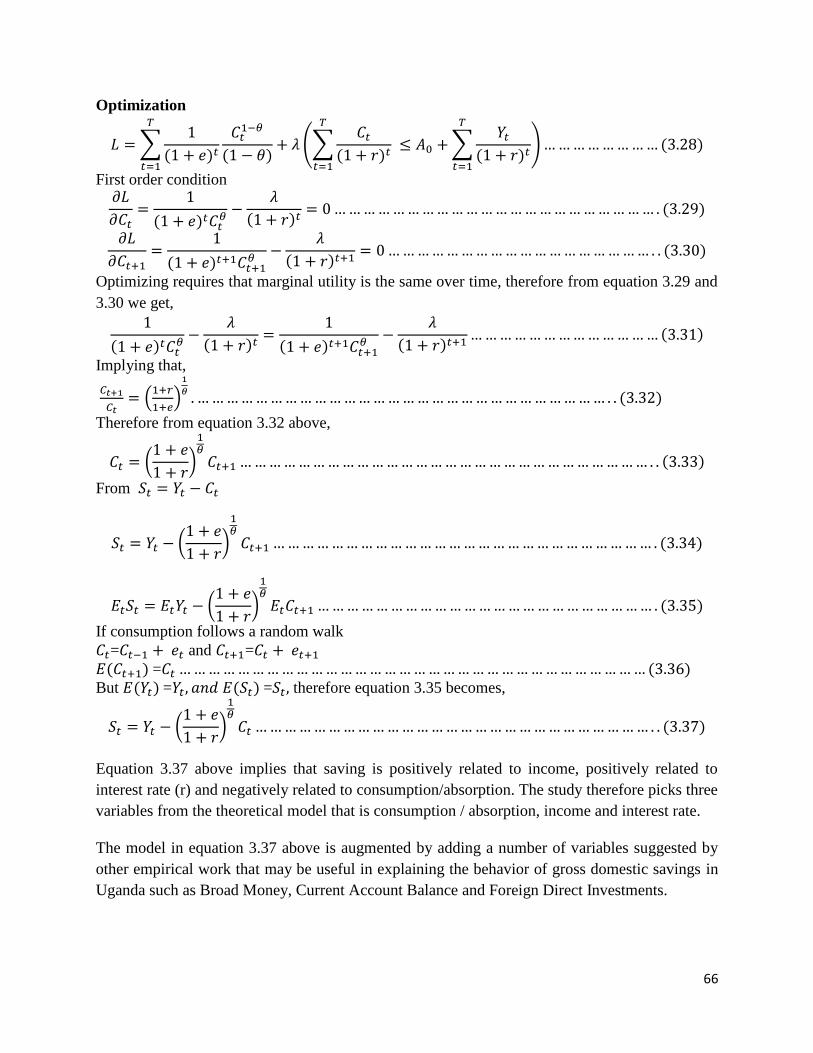
66
Optimization
∑
( )
( ) (∑
( )
∑
( )
) ( )
First order condition
( )
( ) ( )
( )
( ) ( )
Optimizing requires that marginal utility is the same over time, therefore from equation 3.29 and
3.30 we get,
( )
( )
( )
( ) ( )
Implying that,
(
)
( )
Therefore from equation 3.32 above,
(
)
( )
From
(
)
( )
(
)
( )
If consumption follows a random walk
= and = ( ) = ( ) But ( ) = ( ) = therefore equation 3.35 becomes,
(
)
( )
Equation 3.37 above implies that saving is positively related to income, positively related to
interest rate (r) and negatively related to consumption/absorption. The study therefore picks three
variables from the theoretical model that is consumption / absorption, income and interest rate.
The model in equation 3.37 above is augmented by adding a number of variables suggested by
other empirical work that may be useful in explaining the behavior of gross domestic savings in
Uganda such as Broad Money, Current Account Balance and Foreign Direct Investments.

67
APPENDIX 3: Variable Description and Expected Sign
Variable Definition Expected sign Data source
GDS GDS is the dependent variable. GDS is
defined as the total domestic savings by
Government, firms and households in a
given year. GDS equals GDP less final
consumption expenditure /total
consumption expressed as a percentage
of GDP.
Dependent variable World bank
(WDI
indicators,
2018)
GDPg
World Bank defines GDPg as the
annual percentage growth rate of GDP
at market prices based on constant local
Currency. It is a measure of economic
growth. GDP is the sum of gross value
added by all resident producers in the
economy plus any product taxes and
minus any subsidies not included in the
value of the products. GDPg is a
percentage.
A positive relationship is expected
between GDP growth rate and GDS
which is in line with predictions of
Lifecycle/ permanent income
hypothesis.
World bank
(WDI
indicators,
2018)
DIR Deposit interest rate is the rate paid by
commercial or similar banks for
demand, time, or savings deposits.
Deposit Interest rate is considered as
one of the financial variables that have
an impact on saving. DIR serves as the
relative price of current consumption in
relation to future consumption. DIR is
measured in percentage.
Classical economists, McKinnon
(1973) and Shaw (1973) all believe
that Savings is an increasing
function of the rate of interest and
therefore a positive relationship is
expected between GDS and DIR.
World bank
(WDI
indicators,
2018)
M2 This measures the degree of
monetization of the economy. It is a
proxy variable for measuring financial
sector and market development. That is,
broad money measures the amount of
monetary assets available in an
economy, accessibility to banking
facilities and extent of credit
opportunity.M2 is expressed as a
percentage of GDP.
Higher monetary aggregates like
M2 include components
like money market securities,
mutual funds and other time
deposits that have higher interest
rates and encourage savings. A
positive relationship is therefore
expected between GDS and M2.
World bank
(WDI
indicators,
2018)

68
CAB CAB is the sum of net exports of goods
and services, factor income from
investments (net primary income) and
financial transfers (interest earnings and
foreign remittances) / net secondary
income. It shows how the external
sector affects gross domestic saving
ratio. CAB is expressed as a percentage
of GDP
Depending on whether Uganda has
a Current Account Deficit or
Current Account Surplus, the
relationship between GDS and
CAB maybe negative or positive.
World bank
(WDI
indicators,
2018)
GNE GNE is absorption in the economy. It is
the combined amount of all expenses
both private and public excluding
exports. It is the sum of household final
consumption expenditure, government
final consumption expenditure and
gross capital formation. GNE is
expressed as a percentage of GDP.
Keynes, 1936 postulates that saving
is a negative function of
consumption/ absorption. That is an
increase in consumption leads to an
automatic reduction in savings. A
negative relationship is expected
between GNE and GDS.
World bank
(WDI
indicators,
2018)
FDI This series shows net inflows that is,
new investment inflows less dis-
investment in the Uganda from foreign
investors, expressed as a percentage of
GDP.
An increase in FDI leads to an
increase in domestic investments
which leads to an increase in
employment opportunities and
hence people‘s incomes which in
turn leads to increased savings. A
positive relationship between FDI
and GDS is expected.
World bank
(WDI
indicators,
2018)

69
APPENDIX 4: Graphical plots of the variables
Source: Own compilation based on the World Bank Data
05
10
15
20
GD
S
1980 1990 2000 2010 2020year
GDS
010
20
30
40
DIR
1980 1990 2000 2010 2020year
DIR
-20
-10
010
GD
Pg
1980 1990 2000 2010 2020year
GDPg
510
15
20
25
M2
1980 1990 2000 2010 2020year
M2

70
Source: Own compilation based on the World Bank Data
-10
-50
5
CA
B
1980 1990 2000 2010 2020year
CAB
02
46
FD
I
1980 1990 2000 2010 2020year
FDI100
105
110
115
GN
E
1980 1990 2000 2010 2020year
GNE

71
APPENDIX 5: Variance inflation factors results (VIF)
Source: Own computation using Stata 13
Note: Data used is from World Development Indicators (WB, 2018)
Variable VIF 1/VIF
FDI 7.37 0.135639
M2 6.34 0.157841
GDS
L1. 6.33 0.158065
GDPg 5.56 0.179796
DIR 4.41 0.226703
CAB 3.79 0.263624
GNE 3.59 0.278436
GDPg
D1. 3.15 0.216942
CAB
D1. 2.84 0.352053
LD 2.32 0.431499
DIR
D1. 1.98 0.504192
CAB
L2D. 1.59 0.628472
Mean VIF 4.11

72
APPENDIX 6: CUSUM and CUSUMsq control charts
CU
SU
M
year
CUSUM
1988 2017
0 0
CU
SU
M s
quare
d
year
CUSUM squared
1988 2017
0
1