determinants of gdp growth and the impact of … of gdp growth and the impact of austerity . arvind...

Determinants of GDP Growth and the Impact of Austerity

Arvind Jadhav University of Dallas

James P. Neelankavil

Hofstra University

David Andrews University of Dallas

Most industrialized countries are facing slower growth rates, higher unemployment levels, and unnamable national debt as a percentage of GDP and consequently incurring a high cost of servicing this debt. Among the various solutions suggested to reduce the debt burden is to undertake austerity measures to improve fiscal balance and, hence, potentially reduce debt. Growth and austerity programs appear to be inversely related during periods of downturn and slow economic recovery. It has been shown that during a period of sustained upswing, both objectives are positively correlated as higher growth enables higher austerity. To date, studies that have attempted to suggest the feasibility of attaining growth through various programs including austerity during rising national debt have not conclusively shown that this is an attainable objective for policy makers. In this paper we attempt to show that there are initiatives that government’s can implement given the right timing and well-planned initiatives could offer a reasonably successful solution. INTRODUCTION

A number of countries are making a serious effort to undertake policies to stimulate the growth of their economies. Developed countries are interested in growth in order to recover from the recession of 2008–2009 and developing countries want their economies to grow to benefit from the rewards of an industrialized economy. However, most of the developed countries are also facing an unsustainable level of national debt as a percentage of GDP and consequently incurring a high cost of servicing this debt. Among the various solutions suggested to reduce the debt burden is to undertake austerity measures to improve fiscal balance and, hence, potentially reduce debt. Growth and austerity appear to be inversely related during periods of downturn and slow economic recovery, mainly due to political pressure. It has been shown that during a period of sustained upswing, both objectives are positively correlated, that is, higher growth enables higher austerity.

Journal of Applied Business and Economics vol. 15(1) 2013 15

BACKGROUND

The growth of real GDP is a macro measure of economic growth, but it does not take into account the benefits derived by various sectors of the economy. If the growth is shared by all income groups, a balance between consumption and investment can be attained. If growth benefits higher-income segments disproportionately, consumption may not increase significantly and an increase in investment may be delayed. The factors that induce an economy’s growth also change with the economy’s changing structure. The measures that provide an impetus to an industrial economy may not be the same as those that stimulate a service economy. Growth within a country also depends on global economic conditions to the extent that a country’s economy is dependent on foreign trade. Austerity implies a reduction in fiscal deficits, primarily through expense reductions. A major reason for increases in government expenses is “entitlements,” comprised of social welfare programs such as health care, social security, and pensions. Interest groups often lobby for maintaining or increasing preferential treatment of selected sectors, thereby necessitating a reduction in services essential for long-term growth. Empirically, governments have not decreased expenditures when the economy is in a growth stage. In addition, the political will to increase revenues in times of higher deficit is found to be lacking. Interest groups often prevent the restructuring of the tax code, which could soften the revenue decrease during recessions and increase receipts during growth without requiring increases in tax rates. This paper attempts to determine the critical factors that affect an economy’s growth and determine if austerity programs positively impact economic growth. A balanced approach for the implementation of growth and austerity measures is suggested on the basis of a country’s economic structure. The analysis includes theoretical developments beginning with the Cobb-Douglas function and an empirical analysis that applies structural vector auto regression. DEFINITION OF GROWTH

The commonly accepted indicator of an economy’s growth is the change in a country’s real GDP. True growth is measured by a secular trend in real GDP. Hence, measuring real growth requires removal of cyclical movements from the data to eliminate fluctuations caused by business cycles. Some economists believe that unless technological (and productivity) growth outpaces the rate of resource depletion, secular growth reaches a steady state and the rate of growth stagnates at the steady state rate. This partly explains why developing economies grow at a rate faster than developed economies do. Up to time t, developing economies initially grow faster due to the availability of greater resources per labor input and to the faster pace of technological developments as shown by dotted line in Chart 1. After this period, all economies are expected to experience the steady state growth rate. This rate represents a combined effect of diminishing returns on per capita resources and technological enhancements (see Figure 1).

16 Journal of Applied Business and Economics vol. 15(1) 2013

FIGURE 1 REAL GDP GROWTH RATE FOR DEVELOPED AND DEVELOPING COUNTRIES

Real GDP growth rate

Time t

LITERATURE REVIEW

Stabilization of the economy is policymakers’ primary goal during periods of severe recession. But stabilization has significant distributional implications; for example, tax increases to eliminate a large budget deficit leads to jockeying for favorable position among various interest groups. For instance, some socioeconomic groups may attempt to shift the burden of stabilization onto other groups. Thus, the process leading to stabilization becomes a war of attrition, with each group attempting to wait for the other group to concede. Implementation of the stabilization policy occurs when one group concedes and bears a disproportionate share of the burden. This scenario in practice is difficult to achieve; hence, austerity programs become ineffective (Alesina and Drazen, 1991). Moreover, in exploring the difficulties of using austerity programs for achieving economic stabilization during economic downturns, Boyer concluded that these programs fail because of four wrongly held assumptions. First, is the false diagnosis that the present crisis is the outcome of a lax public spending policy, when it could be the outcome of a private credit–led speculative boom. Second, is the possibility of so-called expansionary fiscal contractions, which neglects the short-term negative effects on domestic demand. Third, is the assumption that all the countries in the European Union (EU) are the same and hence that one prescription should fit all. Fourth, is that the spillover effect will hold, that is, that a country that is doing well might resuscitate an inefficient one (Boyer, 2012). According to Brown, based on his study of twenty-five European countries, for austerity programs to work, they should be combined with increase in investments (Brown, 2012).

Austerity can be defined as a deliberate process undertaken by a government to reduce national debt. The direct impact of such a measure is elimination of selected government programs and a reduction in financial support of a few private sector projects. The result is inevitably an increase in the unemployment rate and a slowdown in the GDP growth rate. The impact is proportional to the public sector share of GDP. Austerity is incorporated in this analysis through reduction in debt-to-GDP ratio that is based more on government expense reduction and less on revenue increase. Empirical results from EU countries that have implemented austerity measures support this premise. According to Eurostat, the Eurozone unemployment rate hit a record high of 12.2 percent in April, 2013 with 19.4 million people out of work. The unemployment rate in Greece and Spain exceeded 25 percent according to Eurostat.

In spite of its unproven record, austerity programs are policymakers’ quick fix options during times of economic crisis. Research studies that have focused on the recent economic crisis, especially among EU countries, have further validated the implementation of austerity programs during severe economic downturns. But the evidence emerging from the EU example is not at all positive. For example, a study based on the recent austerity program adopted by the UK government for its recovery suggests that the recovery will take significantly longer than the political cycle, that social impacts will be greater than


expected, and that there is excessive optimism in some of the strategic tools being adopted in the UK's deficit recovery (Murray et al., 2012). Similarly, Gros and Maurer report that OECD estimates for the UK suggest that austerity will lead to another recession, which in turn may lead to a higher debt-to-GDP ratio than before (Gros and Maurer, 2012).

If the objective of policymakers were simply to achieve economic growth, there are a number of research studies that have identified specific factors that has shown to have a positive impact on the growth of an economy. Among the theories on economic growth, the one that seems to be accepted by many is the one proposed by Schumpeter. Schumpeterian theory suggests that economic growth is driven by quality-improving innovations, hence the importance of technology. Similarly, in analyzing various theories of economic growth, Nelson and Winter argue for technological change and dynamic competition, encompassing several Schumpeterian ideas to achieve economic growth. They suggest long-term solutions for long-term economic growth (Nelson and Winter, 1974). A study by Aghion also seems to support the idea that the best way to stimulate economic growth is through quality-improving innovations. The downside of the development through technological innovations is that it might contribute to income inequality among the developed economies, as they reward people with education at the cost of those with less education (Aghion, 2002)

A few researchers have also made a strong argument for the importance of human capital development in achieving economic growth. Research in this area has shown that human capital development attained through higher education can significantly contribute to higher economic growth. Using Bayesian averaging classical estimates, Sala-i-Martin, et al., were able to narrow the critical explanatory variables of economic growth from a total of sixty-seven to just three key variables. These three variables are relative price of investment, primary school enrollment, and initial level of real GDP (Sala-i-Martin et al., 2004). In a study of thirty-seven developing countries, Neelankavil, et al., demonstrated that investment in human capital was one of the three key variables that influenced real GDP over the long term, the other two being increased trade, and monetary and fiscal policy (Neelankavil et al., 2011). Similarly, in a major large-scale study covering many countries, Hanushek and Kimko found that labor-force quality, interpreted from international mathematics and science test scores, was strongly related to economic growth (Hanushek and Kimko, 2000). Lastly, in his study of public spending between education and infrastructure investments, Agénor found that the growth-maximizing share of investment in infrastructure depended on the productiveness of investments in educational technology (Agénor, 1978).

A further extension to the neoclassical theory of economic growth proposed by Harrod (1939) and Domar (1946) suggests that factors such as multiplier, accelerator, and capital efficiencies are all useful short-term tools that could be applied to achieving economic growth. Using the Harrod-Domar model for explaining economic growth, Solow concluded that the marginal productivity equation determines the time path of real wage rate (Solow, 1956). At the opposite end of the spectrum, Ayres argues that economic development is achieved through the interaction of three entities: the state, the society, and the market (Ayres, 1998). He does, however, support the Schumpeterian idea of technology’s effect on economic growth.

In recent years, other factors of economic growth have been suggested, including mechanics of growth, income equality, efficiency, FDI flows, and so on. Of the factors and theories proposed to explain economic growth, the mechanics of growth theory is one of the most difficult to apply. The basic mechanics growth theory is derived from the sciences, specifically, mathematics and physics. Whereas, economics is not necessarily driven by rationality or logic; human psychology also enters the equation. As concluded by Grattan-Guinness, “theories in economics, whether mathematical or not, do not emulate mechanics or mathematical physics” (Grattan-Guinness, 2010). On the other hand, using mechanics as an operational system definitely has some value in economics, especially in explaining growth. For example, Lucas used the mechanical approach in testing three models of growth, namely, a model emphasizing physical capital accumulation and technological change, a model emphasizing human capital accumulation through schooling, and a model emphasizing specialized human capital accumulation through learning by doing. He concluded that each model showed some impact on economic growth


(Lucas, 1988). Similarly, Dutta used the mechanics principle to study the diffusion of competition, infrastructure, and literacy levels that might be helpful in explaining economic development (Dutta, 2004).

Income inequality is another factor appears in a few studies of economic growth (Shin, 2012; Stevans, 2012; Poveda, 2011; Forbes, 2000; Barro, 1999; Deininger and Squire, 1998). Poveda makes a strong argument for reducing income inequality, using the Colombian economy as evidence. His study showed that economic development and growth could be achieved most effectively through a decrease in poverty, an increase in equality, a reduction in violence, and improved security (Poveda, 2011). On the other hand, many studies have shown that income inequality either is not a factor or in some cases could be a negative factor. In a study of economic growth, Shin found that income can be viewed as having both a positive and a negative effect on growth (Shin, 2012). That is, higher inequality can retard growth in the early stage of economic development and can encourage growth in a near steady state. In a study of the U.S. economy, Stevans found no empirical evidence to support the equity versus efficiency hypothesis, that is, the assumption that economic incentives are necessary for capital accumulation and growth. In fact, he discovered that in most cases, inequality has had little or no impact on movements in U.S. capital stock, net investment, and consequently economic growth (Stevans, 2012). Hence, from a practical standpoint, countries (especially developing countries) should be careful in utilizing income inequality as a factor in stimulating economic growth.

Some researchers have looked at equality in comparison to efficiency. In one such study, Berg and Ostry found that a trade-off between efficiency and equality may not exist in growth situations, especially in the long term. They note that there are countries that find that improving equality is a way to improve efficiency and achieve more sustainable long-run growth (Berg and Ostry, 2011). In fact, after reviewing a vast body of research, Jiménez-Buedo concluded that the literature shows conflicting results in terms of equality and efficiency. In her study of the Colombian economy, she argues that the efficiency and equality paradigm is better analyzed through the social sciences (Jiménez-Buedo, 2011). Finally, one way of looking at economic development and income inequality might be as the consequences of transaction efficiency (Wenli, 2006). If this is true, then it can be argued that there is no systematic relationship between economic growth and inequality.

In a different vein, Barro explored the relationship between the differences in current GDP/capita and potential GDP/capita. In a study of 100 countries over a 30 year period between 1960 and 1990, Barro concluded that the greater the difference between current GDP/capita and the potential GDP/capita, the faster is the growth of an economy. This also explains why less developed countries grow at a faster rate than developed countries. Moreover, Barro’s study shows that a reduction in the growth rate by 0.2 to 0.3% per year would result in a higher inflation rate of 10% which would reduce the level of real GDP by 4 to 7 percent over a 30 year period (Barro, 1996).

The literature review seems to indicate that austerity programs are the first line of defense of policy makers during times of economic crisis. But the experience of the European Union countries demonstrates that the austerity programs are ineffective and in many instances creates more structural imbalances than remedy the problem. Generally speaking, for countries to achieve sustained economic growth, factors that have an impact are technological innovations, investments in human capital, and increase in international trade. The studies in the area of economic growth, debt-to GDP ratio, factors stimulating economic growth, and austerity programs have proposed partial solutions for the problem of controlling deficits. This paper attempts to address the national debt issue and a prescription to solve it through an empirical analysis of the U.S. economy during the 1970 – 2011 period. OBJECTIVE

The objective of this paper is to analyze the U.S. economy over a 41 year period for the years 1970 to 2011 to analyze its growth in the context of the buildup of the deficits and the austerity policies that were adopted during this period. Specifically, we attempt to determine if following an austerity program in times of economic downturn reduces national debt.


METHODOLOGY

The methodology for reduction in national debt was outlined in an IMF study that proposed an adjustment process based on the relationship between fiscal balance and debt-to-GDP ratio (IMF, 2010). The debt dynamics equation used in IMF analysis to determine the fiscal adjustment required to bring the debt-to-GDP ratio to a set target ratio is as follows:

∆𝒅𝒕 = −𝒑𝒃𝒕 + (𝒓𝑫−𝒈)𝟏+𝒈

𝒅t-1

Where 𝑑𝑡 is gross debt-to-GDP ratio in period t; 𝑝𝑏𝑡 represents fiscal deficit plus net interest payments in period t; 𝑟𝐷 is the nominal interest rate on national debt; 𝑔 stands for nominal GDP growth rate; and 𝑑t–1 denotes the debt in the prior period. The two key determinants of the fiscal adjustment are the interest rate and growth differential 𝑟𝐷 − 𝑔 , and the initial debt represented by 𝑑t–1. It appears that both 𝑟𝐷 and 𝑔 are positively correlated, and both contain an inflation rate component. In the event the differential is equal to zero, the equation reduces to an identity without any additional fiscal adjustment determinant. If the differential is positive, the fiscal adjustment needed to reach the target debt-to-GDP ratio is progressively higher. It is clear that when the differential is negative, meaning the nominal growth of GDP is higher than the nominal interest rate on the national debt, the fiscal adjustment is automatic. The equation does not take into account the impact of FDI and the level of private savings, which could have a bearing on interest rates.

During an economy’s growth cycle, inflation is a consequence of an increased rate of growth, where demand outpaces supply of goods and services. Inflation, in turn, causes the interest rate and wages to rise and adds to the cost of production. Increased costs reduce profit margins, leading to a further reduction in supply and starting an inflationary spiral. As a result, demand falls substantially, thus creating an excess of inventories. Thus the inflection point that separates growth from downturn is reached. An empirical study undertaken in 1983 concluded that the correlation between growth and inflation is negative. This is primarily due to the reduced efficiency of factors of production (Fischer, 1983). This was also demonstrated in the literature review section by Barro’s study. Another study, by Smyth, suggests that both the rate of inflation and the change in the rate of inflation reduce GDP growth significantly (Smyth, 1994). That is, inflation reduces the ability of economic agents to operate efficiently in a private enterprise system. THE MODEL

The model is an expanded version of the Cobb-Douglas production function.

𝐺𝐷𝑃 = 𝐴𝐾𝛼𝐿𝛽 Equation 1

This is the Cobb-Douglas production function, where A stands for the level of technology that combines the capital (K), and labor (L) in technology-consistent proportions. The contribution of capital and labor to GDP is given by α and β, respectively. Since

K = f (Gross Private Investment, Foreign Direct Investment, Debt-to-GDP Ratio, Inflation Rate)

And

L = f (Investment per Worker, Gross Domestic Consumption, Exports)


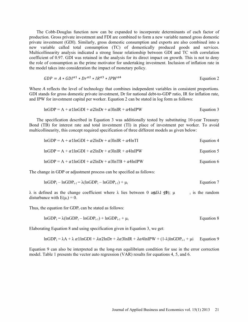
The Cobb-Douglas function now can be expanded to incorporate determinants of each factor of production. Gross private investment and FDI are combined to form a new variable named gross domestic private investment (GDI). Similarly, gross domestic consumption and exports are also combined into a new variable called total consumption (TC) of domestically produced goods and services. Multicollinearity analysis indicated a strong linear relationship between GDI and TC with correlation coefficient of 0.97. GDI was retained in the analysis for its direct impact on growth. This is not to deny the role of consumption as the prime motivator for undertaking investment. Inclusion of inflation rate in the model takes into consideration the impact of monetary policy.

𝐺𝐷𝑃 = 𝐴 ∗ 𝐺𝐷𝐼𝛼1 ∗ 𝐷𝑟𝛼2 ∗ 𝐼𝑅𝛼3 ∗ 𝐼𝑃𝑊𝑎4 Equation 2

Where A reflects the level of technology that combines independent variables in consistent proportions. GDI stands for gross domestic private investment, Dr for national debt-to-GDP ratio, IR for inflation rate, and IPW for investment capital per worker. Equation 2 can be stated in log form as follows:

lnGDP = A + 𝛼1lnGDI + 𝛼2lnDr + 𝛼3lnIR + 𝑎4lnIPW Equation 3

The specification described in Equation 3 was additionally tested by substituting 10-year Treasury Bond (TB) for interest rate and total investment (TI) in place of investment per worker. To avoid multicollinearity, this concept required specification of three different models as given below:

lnGDP = A + 𝛼1lnGDI + 𝛼2lnDr + 𝛼3lnIR + 𝑎4lnTI Equation 4

lnGDP = A + 𝛼1lnGDI + 𝛼2lnDr + 𝛼3lnIR + 𝑎4lnIPW Equation 5

lnGDP = A + 𝛼1lnGDI + 𝛼2lnDr + 𝛼3lnTB + 𝑎4lnIPW Equation 6

The change in GDP or adjustment process can be specified as follows:

lnGDPt – lnGDPt-1 = λ(lnGDPt – lnGDPt-1) + µi Equation 7

λ is defined as the change coefficient where λ lies between 0 and 1 (0≤ λ. ≤1); µ i is the random disturbance with E(µi) = 0. Thus, the equation for GDPt can be stated as follows:

lnGDPt = λ(lnGDPt – lnGDPt-1) + lnGDPt-1 + µi Equation 8 Elaborating Equation 8 and using specification given in Equation 3, we get:

lnGDPt = λA + λ 𝛼1lnGDI + 𝜆𝛼2lnDr + 𝜆𝛼3lnIR + 𝜆𝑎4lnIPW + (1-λ)lnGDPt-1 + µi Equation 9 Equation 9 can also be interpreted as the long-run equilibrium condition for use in the error correction model. Table 1 presents the vector auto regression (VAR) results for equations 4, 5, and 6.


TABLE 1 VAR RESULTS FOR 3 MODELS (EQUATIONS 4 – 6)

VAR MODEL

Variables→ GDP

Debt as % of GDP

Inflation rate (%)

10-year bond yield (%)

Total Inv.

$Billion

Investment per worker

($000) R2

lag 1 $ Billion

1 Coefficient 0.944 6.197 -3.104 359.351 0.9996 t value 29.4 3.0 -0.4 2.3

2 Coefficient 0.953 4.141 -6.402 52.338 0.9997 t value 38.8 2.2 -0.8 2.8 3 Coefficient 0.950 4.562 -6.157 54.281 0.9997

t value 30.3 2.6 10.3 2.5 ANALYSIS

The empirical results from Table 1 identify a set of variables (listed below) that have a significant impact on the economic growth of a country. Interpolated estimates are very close to the actual values for each of the three models. The coefficient of determination for each of the three model results is very high primarily due to inclusion of the lagged value of GDP.

• Debt as percent of GDP is demonstrably the most significant explanatory variable. The positive sign of the coefficient suggests that the stimulating effects of an increase in debt level reflecting mainly higher level of government spending, will persist at any level of debt. It should be noted that the impact of the level of debt is not direct, but through the impact of the investments by the government and private sector. As an example, if higher government spending leads to higher consumption at both the public and the private levels, it will encourage investments in the private sector. Investment by government in infrastructure will also encourage investments by the private sector in all related activities.

• Taken by itself, the positive causality relationship between debt-to-GDP ratio and the level of GDP appears to create an explosive series (it should be noted that in a VAR analysis with multiple explanatory variables, the coefficients are determined jointly and the impact of coefficient of one variable alone cannot be isolated). The constraints on explosive growth are brought about through consequential effects of increased inflation and an increased bond yield evident through the negative coefficients of these variables. Thus, debt-to-GDP ratio is an ‘instrument’ variable whose impact on the GDP is determined in the context of a given economic environment.

• Domestic private investment, whether measured as total or per worker, directly contributes to growth. Investment per worker embodies innovation emanating from technological advances which is also an important determinant of growth. Investment per worker also implies increased investment in human capital necessitated by technological innovations.

• Lower ‘t’ values for the coefficient of inflation rate can be partly explained by higher variability in historical values. Rate of inflation is a component in determining wage rate and bond yield. Inflation increases the cost of capital as well as the cost of operations. The coefficient of bond


yield has a higher ‘t’ value, thereby making bond yield a more appropriate explanatory variable rather than the inflation rate.

An attempt was made to improve the accuracy of models by addition of Bayesian approach of

incorporating extraneous information. Beginning with the ‘prior’ distribution as computed in the above three models, a ‘posterior’ distribution can be estimated by incorporating external information available from prior studies. The posterior function could be helpful in estimating the point of inflexion in GDP level and debt-to-GDP ratio. The external inputs available for integration in this analysis are based on previous studies as listed below.

• For advanced economies, Reinhart and Rogoff concluded that for a debt-to-GDP ratio between 30 to 90% limits the growth of GDP at a median rate of about 3 percent per year. When the ratio exceeds 90%, GDP growth declines considerably, to about 1.9%. For emerging economies, the median growth rate of GDP stays around 4 to 4.5% at a ratio below 90% and falls to 2.9% when the debt ratio exceeds 90% (Reinhart and Rogoff, 2010). This study has been criticized because of computational errors in empirical analysis and ignoring changing economic regimes.

• The IMF estimates that a 10% increase in the debt-to-GDP ratio will decrease the annual real per capita GDP growth by 0.15% for advanced economies and by 0.2% for emerging economies. A 10% increase in initial debt will also reduce investments by 0.4% of GDP and increase the ten-year bond yield by 2% in advanced economies (IMF, 2010).

• Analyzing the U.S. debt from 1970 through 2011 Jadhav, et al., 2012, identified three variables that have the greatest impact on the economy. These are: fiscal balance, prevailing long term rate of interest, and GDP growth rate. They further suggest that the U.S. should not exceed a national debt to GDP ratio level of 93%.The study also estimates an optimum level of debt to GDP ratio of 65% for the U.S. which could be reached within ten years with strong fiscal policies. The 65% level of debt suggested by Jadhav, et, al., closely corresponds to the ratio of 60% proposed by the IMF for developed countries (Jadhav, et al., 2012).

Bayesian approach, integrating the above extraneous information did not result in determining a

uniquely identifiable solution that is needed in utilizing an error correction model. Bayesian solution produces a posterior density function of α coefficients rather than a point estimate. This results in a set of simultaneous equation without a single unique equilibrium solution. Therefore, the extraneous information available in the three studies noted above (Reinhart and Rogoff, 2010), (IMF, 2010), and (Jadhav, et al., 2012) is integrated in this analysis to illustrate the relationship between debt-to-GDP ratio and growth rate of GDP in Figure 2.

The inflexion point of the curve is based on the optimum debt-to-GDP ratio as estimated in an earlier paper by Jadhav, et al. that suggested for the U.S. economy to maintain a 4% GDP growth level it should not exceed a debt-to GDP ratio of 65% (Jadhav, et al., 2012). The shape of the curve beyond the optimum debt-to-GDP ratio is based on previous studies listed above.

The question is how do austerity measures enter the equation when discussing GDP growth rates and debt-to-GDP ratios? An important lesson about austerity measures could be drawn from some recent research studies on the EU countries that had proposed austerity programs for individual countries as well as for the group as a whole. EU countries’ experience suggests that it is not the level of debt-to-GDP ratio that mattered but the timing and speed of reduction. Austerity measures undertaken prior to an economy resuming a sustained growth creates a new recessionary spiral. The speed of reduction in debt-to-GDP ratio for reaching the target ratio as recommended by the previously mentioned IMF study will have an impact on consumption and subsequently on investment level. Bad timing and excessive speed of reduction of debt could lower the peak of the curve depicted in Figure 2 down towards the X axis and lower the rate of growth of GDP at all levels of debt ratio. The studies on the EU suggest that growth of GDP should be the first priority for country’s to pursue and reduction in national debt should be a long-term objective.


FIGURE 2 DEBT-TO-GDP RATIO AND GDP GROWTH RATE

GDP growth rate

4 –

2 –

Debt-to GDP ratio

Optimum ratio

To further understand the relationship between GDP growth rate and austerity programs, an analysis of the debt-to-GDP ratio and GDP growth rate for selected EU countries for the years 2009 to 2012 was conducted. Based on this analysis it evident that for the EU countries the debt reduction programs were not very successful in stimulating the economy (see Appendix A). It appears that the deficit reduction targets were high, austerity programs were initiated prior to a sustained economic recovery and the growth in debt-to-GDP ratios was not arrested as anticipated. As a result, EU countries suffered lower or even negative rate of growth of GDP during 2011 and 2012. A number of these countries are currently in a double dip recession or on the brink of it. Moreover, unemployment rates have increased in all the EU countries except in Germany, but inflation has fallen in all these countries in 2012 as a result of a reduction in demand resulting from austerity measures.

The evidence from the EU’s policies could be utilized in arriving at a plan for both the timing and speed of fiscal consolidation. The IMF adjustment process quoted earlier in this paper defines the coefficient of prior period debt as (rD-g)/1+g, where rD stands for nominal rate of interest on government debt and g denotes nominal GDP growth. This formulation and recent experience of European countries suggests that austerity measures should not be implemented until g shows a sustained increase and exceeds rD. An additional advantage of such timing is that the required adjustment; i.e., reduction in annual budgetary deficits; will be smaller due to revenue increase brought about by increased rate of growth of GDP. There is not enough historical data to determine the speed of fiscal adjustment towards a target debt-to-GDP ratio. The target ratio and the period of adjustment are still in the realm of subjective judgments, although an estimate of an optimum ratio consistent with full employment conditions was presented in a recent study (Jadhav, et. al., 2012). Based on the recent experience of European countries, it appears that the rate of annual fiscal adjustment given in percent of GDP should be increased progressively but not to exceed g, the average expected GDP growth rate over the period of adjustment. This formulation in itself can help determine the period over which the fiscal adjustment can be stretched to bring down the current debt-to-GDP ratio to the target ratio without sacrificing economic growth.


CONCLUSIONS

The analysis of the U.S. economic data including debt as a percentage of GDP, inflation rate, investments, 10-year bond yield, and investments per worker for the years 1970 through 2011 using VAR analysis provide some interesting findings. The analysis suggests that while the fiscal deficits originated as a stop gap arrangement, over a period of time they have become an accepted source of financing government expenses that are not covered by revenues even during periods of economic growth. The specific findings of this paper are:

• An increase in national debt, measured as percent of GDP, can stimulate growth of the economy in recessionary periods by filling the void left by a decline in private consumption and investment. However, beyond an optimum level of debt, the rate of growth of the economy will diminish.

• The reduction in growth rate beyond the optimum level of debt is the result of the consequential effects of increased inflation, increased bond yield, and increased wage rate leading to an increase in the marginal private cost of operations of businesses. This translates into a decline in total investments. However, an increase in productivity through higher investment per worker as a result of technological innovations can offset some of the decline in the rate of growth. Financial policy impacts both inflation and rate of interest. Federal Reserve Bank actions enter into the analysis through these variables.

• Based on the EU’s experience, austerity initiatives and other reduction in national debt programs require establishing a country specific long term objective of the target/optimal level of debt ratio. Austerity programs should include a balance between revenue increase and expense reduction. Such programs should be combined with a progressive fiscal adjustment formula as opposed to a flat annual rate of reduction in annual deficits. The fiscal adjustment should not be initiated until after the economy experiences a sustained period of growth.

REFERENCES Agénor, Pierre-Richard, (1978), “Schooling and public capital in a model of endogenous growth,” Economica 78, no. 309: 108–132. Aghion, Philippe, (2002), “Schumpeterian growth theory and dynamics of income equality,” Econometrica 70, no. 3: 855–882. Alesina, Alberto, and Allan Drazen, (1991), “Why are stabilizations delayed?” American Economic Review 81, no. 5: 1170–1188. Ayres, Robert U., (1998), Turning Point: An End of the Growth Paradigm. New York: St. Martin's Press. Barro, Robert J., (1996), “Inflation and growth,” Review, Federal Reserve Bank of St. Louis, (May/June): 153–169. Barro, Robert J., (1999), “Inequality, growth, and investment,” NBER Working Paper 7038. Berg, Andrew G., and Jonathan D. Ostry, (2011), “Inequality and unsustainable growth: Two sides of the same coin?” IMF Staff Discussion Note, April 8, SDN/11/08. Bureau of Labor Statistics, (2012), Bureau of Labor Statistics Report (January 27). Boyer, Robert, (2012), “The four fallacies of contemporary austerity policies: The lost Keynesian legacy,” Cambridge Journal of Economics 36, no. 1: 283–312.


Brown, Duncan, (2012), “European rewards in an era of austerity: Shifting the balance from the past to the future,” Compensation and Benefits Review 44, no. 3: 131–144. Deininger, K., and L. Squire, (1998), “New ways of looking at old issues: Inequality and growth,” Journal of Development Economics 57, no. 2: 259–287. Domar, Evsey, (1946), “Capital expansion, rate of growth, and employment, Econometrica, 14, no. 2: 137-147. Dutta, Amitava, (2004), “The mechanics of growth: A developing-country perspective,” International Journal of Electronic Commerce 9, no. 2: 143–165. Fischer, Stanley, (1983), “Inflation and growth,” NBER Working Paper 1235 (November). Forbes Kristin J., (2000), “A reassessment of the relationship between inequality and growth,” American Economic Review 90, no. 4: 869–887. Grattan-Guinness, Ivor, (2010), “How influential was mechanics in the development of neoclassical economics? A small example of a large question,” International Journal of History and Economic Thought 32, no. 4: 531–558. Gros, Daniel, and Rainer Maurer, (2012), “Can austerity be self-defeating?” Intereconomics 47, no. 3: 175–184. Hanushek, Eric A., and Dennis D. Kimko, (2000), “Schooling, labor force quality, and growth of nations,” American Economic Review 90, no. 5: 1184–1208. Harrod, Roy, F., (1939), “An essay in dynamic theory, The Economic Journal, 49 (March): 14-33. Jadhav, Arvind G., Neelankavil, James P, and Andrews David (2012), “Maximum Sustainable Level of National Debt,” Journal of Accounting and Finance, 12(2): 51-64. Jiménez-Buedo, María, (2011), “The political uses of some economic ideas: The trade-off between efficiency and equality,” American Journal of Economics and Sociology 70, no. 4: 1029–1052. Lucas, Robert, Jr., (1988), “On the mechanics of economic development,” Journal of Monetary Economics 22, no. 1: 3–42. Murray, Gordon J., Andrew Erridge, and Neil Rimmer, (2012), “International lessons on austerity strategy,” International Journal of Public Sector Management 25, no. 4: 248–259. Neelankavil, J.P., L. Stevans, and F.L. Roman, (2011), “Correlates of economic growth for developing countries: A panel cointegration approach,” International Review of Applied Economics 26, no. 1: 83–96. Staff of the Fiscal Affairs Department, International Monetary Fund, (2010), “Navigating the fiscal challenges ahead,” IMF Fiscal Monitor (May 14). Nelson, Richard R., and Sidney G. Winter, (1974), “Neoclassical vs. evolutionary theories of economic growth: Critique and prospectus,” Economic Journal 84, no. 336: 886–905.


Poveda, Alexander Cotte, (2011), “Economic development and growth in Colombia: An empirical analysis with super-efficiency DEA and panel data models,” Socio-Economic Planning Sciences 45, no. 4: 154–164. Reinhart, Carmen M., and Kenneth S. Rogoff, (2010), “Growth in time of debt,” American Economic Review 100, no. 2: 573–578. Sala-i-Martin, Xavier, Gernot Doppelhofer, and Ronald I. Miller, (2004), “Determinants of long-term growth: A Bayesian averaging of classical estimates,” American Economic Review 94, no. 4: 813–835. Shin, Inyong, (2012), “Income inequality and economic growth, Economic Modelling, 29, no. 5:2049-2057. Smyth, David J., (1994), “Inflation and growth,” Journal of Macroeconomics 16, no. 2: 261–270. Solow, Robert M., (1956), “A contribution to the theory of economic growth,” Quarterly Journal of Economics 70, no. 1: 65–94. Stevans, Lonnie K., (2012), “Income inequality and economic incentives: Is there an equity-efficiency tradeoff”? Research in Economics 66, no. 2: 149–160. Stiglitz, Joseph E., (2012), The Price of Inequality. New York: W.W. Norton. Staff of the Fiscal Affairs Department, International Monetary Fund, (2009), “The state of public finances cross-country,” IMF Fiscal Monitor, November 3. OECD, (2011), “Trade union density,” OECD.StatExtracts. Wenli, Cheng, (2006), “A new perspective on economic development and income inequality,” Economic Papers 25, no. 2: 125–130. Wilkinson, Richard G., and Kate Pickett, (2009), The Spirit Level: Why More Equal Societies Almost Always Do Better. London: Allen Lane.


APPENDIX A DEBT-TO-GDP RATIOS AND GDP GROWTH RATES FOR SELECTED EU COUNTRIES

Country/zone Debt-to-GDP ratio GDP growth rate

2009 2010 2011 2012 2009 2010 2011 2012

Eurozone 80.0 85.4 88.0 93.6 -4.4 2.0 1.4 -0.6 France 79.2 82.3 86.0 90.0 -3.1 1.7 1.7 0.0 Germany 74.7 82.4 80.6 83.0 -5.1 4.2 3.0 0.7 Greece 129.0 144.6 165.4 175.7 -3.1 -4.9 -7.1 -6.4 Ireland 64.9 92.2 106.5 117.7 -5.5 -0.8 1.4 0.9 Italy 116.0 118.6 120.1 126.3 -5.5 1.8 0.4 -2.4 Portugal 83.1 93.3 107.8 119.1 -2.9 1.9 -1.6 -3.2 Spain 53.9 61.3 69.1 90.7 -3.7 -0.3 0.4 -1.4 UK 68.0 75.0 81.8 88.7 -4.0 1.8 0.9 0.3 US 89.7 98.6 102.9 107.2 -3.1 2.4 1.8 2.2 Japan 210.2 215.3 229.6 236.6 -5.5 4.7 -0.6 1.9

Country/zone

Unemploy-ment rate

Inflation rate

2009 2010 2011 2012 2009 2010 2011 2012 Eurozone 9.0 10.1 10.7 11.8 0.3 1.6 2.7 2.5 France 9.5 9.7 9.9 10.6 0.1 2.0 2.3 2.2 Germany 7.8 7.1 5.6 5.4 0.2 1.2 2.5 2.1 Greece 9.5 12.6 21.3 26.1 1.3 1.6 3.1 1.0 Ireland 11.9 13.7 15.0 14.0 -1.7 1.2 1.2 1.9 Italy 7.8 8.4 9.5 11.4 0.8 1.7 2.9 3.3 Portugal 9.6 11.0 14.6 17.3 -0.9 1.6 3.6 2.8 Spain 18.0 20.1 23.1 26.2 -0.2 4.7 3.1 2.4 UK 7.6 7.8 8.3 7.7 2.2 1.4 4.5 2.8 US 9.3 9.6 8.5 7.8 -0.4 3.3 2.9 1.8 Japan 5.1 5.1 4.5 4.3 -1.4 1.6 0.7 -0.4

Source: EUROSTAT and IMF Statistics.


determinants of gdp growth and the impact of … of gdp growth and the impact of austerity . arvind...

Documents