determinants of exchange rate volatility in south africa

Determinants of Exchange Rate

Volatility in South Africa

Desireé Dewing

201005381

A thesis submitted in fulfilment of the requirements for the degree of

Master of Commerce

In

Economics

In the Faculty of Management and Commerce

At the

University of Fort Hare

East London

Supervisor: Professor A. Tsegaye

2015

i

ABSTRACT

The rand is observed to have experienced volatility in recent times, which was particularly

pronounced during times of crises such as the East Asian Crisis of 1998 and the global

financial crisis of 2008. The purpose of this study is to identify key macroeconomic variables

that determine exchange rate volatility in South Africa, and to also determine the contribution

of each of these variables to volatility. The study makes use of quarterly data from 1994 to

2014. Volatility is measured by means of a generalized autoregressive conditional

heteroscedasticity approach. Estimation techniques employed include the Johansen Co-

integration and vector error correction model. Impulse response and variance decomposition

analysis revealed that interest rate differentials account for most of the variation in exchange

rate volatility (36%), followed by inflation rate differentials (31%), economic growth (3.5%),

trade openness (0.45%), money supply (0.25%) and government spending (0.03%). Interest

rate differentials and inflation rate differentials thus account for 67% of the 71% variation in

exchange rate volatility in South Africa, with trade openness, money supply and government

spending all being of low levels of significance. The large impact that monetary variables

have on exchange rate volatility implies that policymakers should maintain sound monetary

policies, ensuring that large unwarranted increases in interest rates do not occur in the bid to

control inflation.

.

ii

DECLARATIONS

On originality of work

I, the undersigned, …………………., student number……………, hereby declare that the

dissertation is my own original work, and that it has not been submitted, and will not be

presented at any other University for a similar or any other degree award.

Date: ……………………………….

Signature:………………………………….

On plagiarism

I, ………………….,, the undersigned, student number……………, hereby declare that I am

fully aware of the University of Fort Hare’s policy on plagiarism and I have taken every

precaution to comply with the regulations.

Signature:………………………………….

On research ethics clearance

I, ………………….,, the undersigned, student number……………, hereby declare that I am

fully aware of the University of Fort Hare’s policy on research ethics and I have taken every

precaution to comply with the regulations. I have obtained an ethical clearance certificate

from the University of Fort Hare’s Research Ethics Committee and my reference number is

the following:……..N/A………

Signature:………………………………….

iii

ACKNOWLEDGEMENTS

Firstly, I wish to extend my sincere thanks and gratitude to my supervisor, Professor Asrat

Tsegaye. Thank you Professor Tsegaye for continuously providing me with encouragement. I

have been fortunate to have been placed under the supervision of such an inspirational

mentor. Thank you for always responding quickly to my queries and for the many late nights

you have spent reading through draft chapters.

I must express my thanks to all the members of staff at the University of Fort Hare,

Department of Economics, for their support. Special mention is made to my friend and

colleague in the department, Forget Kapingura, for his invaluable advice and assistance.

Thanks also to Mishi Syden and Sibanisezwe Khumalo for their input into this research.

To my partner, William Hunter, thank you for your ongoing support and patience during this

process. I am grateful to my parents, Hansie and Heather Dewing, for teaching me that

anything is possible through hard work and dedication.

The financial assistance of the National Research Foundation (NRF) towards this research is

hereby acknowledged. Opinions expressed and conclusions arrived at, are those of the author

and are not necessarily to be attributed to the NRF.

iv

Table of Contents ABSTRACT……………………………………………………………………………………i

DECLARATIONS………………………………………………………………………….…ii

ACKNOWLEDGEMENTS…………………………………………………………………..iii

LIST OF FIGURES…………………………………………………………………………viii

LIST OF TABLES…………………………………………………………………………..viii

ACRONYMS AND ABBREVIATIONS……………………………………………………...x

CHAPTER ONE: INTRODUCTION TO THE RESEARCH ISSUE

1.1. Background to the Study ..................................................................................................... 1

1.2. Statement of the Problem .................................................................................................... 2

1.3. Objectives of the Study ....................................................................................................... 4

1.4. Hypotheses .......................................................................................................................... 4

1.5. Significance of the Study .................................................................................................... 4

1.6. Organization of the Study ................................................................................................... 5

CHAPTER TWO: AN OVERVIEW OF THE BEHAVIOUR OF THE REAL EFFECTIVE

EXCHANGE RATE AND RELATED VARIABLES

2.1. Introduction ......................................................................................................................... 6

2.2. Real Effective Exchange Rate (REER) of South Africa ..................................................... 6

2.3. Government Expenditure .................................................................................................. 10

2.4. Money Supply ................................................................................................................... 13

2.5. Trade Openness ................................................................................................................. 15

2.6. Economic Growth ............................................................................................................. 17

2.7. Inflation Rate Differential ................................................................................................. 19

2.7.1. Inflation Rate Performance (1994-2000) ................................................................... 21




2.8. Real Interest Rate (RIR) Differential ................................................................................ 25

2.8.1. Performance of Real Interest Rate (1994-2000) ........................................................ 26



v

2.8.4. Performance of Real Interest Rate (2011-2014) ......................................................... 28

2.9. Conclusion ........................................................................................................................ 29

CHAPTER THREE: LITERATURE REVIEW

3.1. Introduction ....................................................................................................................... 30

3.2. Exchange Rate Definitions ............................................................................................... 30

3.2.1. Nominal Exchange Rate ............................................................................................. 30

3.2.2. Nominal Effective Exchange Rate ............................................................................. 31

3.2.3. Real Exchange Rate ................................................................................................... 32

3.2.4. Real Effective Exchange Rate .................................................................................... 34

3.3. Theoretical Literature Review .......................................................................................... 35

3.3.1. Purchasing Power Parity Theories ............................................................................. 35

3.3.1.1. Absolute Purchasing Power Parity Theory .......................................................... 35

3.3.1.2. Relative Purchasing Power Parity Theory ........................................................... 36

3.3.2. The Monetary Models ................................................................................................ 37

3.3.2.1. The Flexible Price Monetary Model .................................................................... 38

3.3.2.2. The Dornbusch Sticky Price Monetary Model .................................................... 40

3.3.2.3. The Frankel Real Interest Rate Differential Model ............................................. 42

3.3.3. The Balance of Payments Approaches ....................................................................... 43

3.3.3.1 Elasticities Approach ............................................................................................ 43

3.3.3.2. Absorption Approach .......................................................................................... 44

3.3.4. Portfolio Balance Approach ....................................................................................... 45

3.4. Empirical Literature Review ............................................................................................. 46

3.5. Assessment of the Literature Obtained ............................................................................. 51

CHAPTER FOUR: RESEARCH METHODOLOGY

4.1. Introduction ....................................................................................................................... 53

4.2. Model Specification .......................................................................................................... 53

4.3. Definition of Variables and a Priori Expectations ............................................................. 54

4.4. Review of Estimation Techniques ..................................................................................... 59

4.4.1. Volatility Measures ..................................................................................................... 59

4.4.2. Testing for Stationarity ............................................................................................... 60

4.4.2.1. Graphical Analysis .............................................................................................. 61

vi

4.4.2.2. Dickey-Fuller Test ............................................................................................... 61

4.4.2.3. Augmented-Dickey Fuller Test ........................................................................... 62

4.4.2.4. Phillips-Perron Test ............................................................................................. 62

4.4.3. Co-integration Analysis .............................................................................................. 63

4.4.3.1. Johansen Co-integration Approach ..................................................................... 63

4.4.3.2. Vector Error Correction Model ........................................................................... 65

4.4.4. Diagnostic Tests ......................................................................................................... 66

4.4.4.1. Serial Correlation ................................................................................................. 67

4.4.4.2. Whites Heteroscedasticity Test ........................................................................... 67

4.4.4.3. Residual Normality Test ...................................................................................... 67

4.4.4.4. Impulse Response Analysis ................................................................................. 68

4.4.4.5. Variance Decomposition ..................................................................................... 68

4.5. Conclusion ........................................................................................................................ 68

CHAPTER FIVE: EMPIRICAL ANALYSIS AND FINDINGS

5.1. Introduction ....................................................................................................................... 70

5.2. Descriptive Statistics ......................................................................................................... 70

5.3. Stationarity Test ................................................................................................................ 71

5.3.1. Graphical Analysis ..................................................................................................... 71

5.3.2. Augmented Dickey Fuller Test and Phillips Perron Test ............................................ 72

5.4. Co-integration Test ............................................................................................................ 75

5.4.1. Order of Integration .................................................................................................... 75

5.4.2. Optimal Lag Length Selection Criteria ...................................................................... 76

5.4.3. Deterministic Trend Assumption ................................................................................ 76

5.4.4. Determination of the Rank of ∏ ................................................................................ 77

5.5. Vector Error Correction Modelling ................................................................................... 78

5.6. Diagnostic Checks ............................................................................................................ 81

5.6.1. AR Roots Graph ......................................................................................................... 82

5.6.2. Serial Correlation ....................................................................................................... 82

5.6.3. Heteroscedasticity ...................................................................................................... 82

5.6.4. Normality ................................................................................................................... 83

5.7. Impulse Response Analysis............................................................................................... 83

5.8. Variance Decomposition Analysis .................................................................................... 84

vii

5.9. Conclusion ........................................................................................................................ 85

CHAPTER SIX: SUMMARY, CONCLUSIONS, POLICY IMPLICATIONS AND

RECOMMENDATIONS

6.1. Summary of the Study and Conclusions ........................................................................... 87

6.2. Policy Implications and Recommendations ...................................................................... 89

6.3. Delimitations of the Study and Areas for Further Research ............................................. 90

REFERENCES ........................................................................................................................ 92

APPENDICES………………………………………………………………………………101

viii

LIST OF FIGURES

Figure 2.1: Real Effective Exchange Rate of South Africa (1994-2014)……………………..7

Figure 2.2: National Government Spending % Change for South Africa (1994-2014)……...11

Figure 2.3: Money Supply % Change for South Africa (1994-2014)………………………..13

Figure 2.4: Trade Openness of South Africa (1994-2014) ……………………………….….16

Figure 2.5: Real GDP Performance of South Africa (1994-2014)…………………………...18

Figure 2.6: Inflation Rate Performance for the United States and South Africa (1994-2014).20

Figure 2.7: Inflation Rate Differential and the REER (1994-2014) …………………………21

Figure 2.8: RIR Differential for South Africa and the United States (1994-2014) ………….25

Figure 2.9: RIR Differential and the REER (1994-2014) …………………………………...26

Figure 5.1: Graphical Presentations of the Variables in Level Form ………………………..72

Figure 5.2: Graphical Presentation of the Variables in First Difference Form ……………...75

Figure 5.3: AR Roots Graph ………………………………………………………………...82

Figure 5.4: Impulse Response Results ………………………………………………………84

LIST OF TABLES

Table 5.1: Descriptive Statistics ……………………………………………………………..71

Table 5.2: Unit Root ADF and PP Test Results in Level Form……………………………...73

Table 5.3: Unit Root ADF and PP Test Results in First Difference Form…………………...74

Table 5.4: VAR Lag Selection ………………………………………………………………76

Table 5.5: The Pantula Principle Test Results ………………………………………………77

Table 5.6: Johansen Co-integration Rank Test Results………………………………………78

Table 5.7: Long-run Co-integration Equation Results ………………………………………79

Table 5.8: Short-run Co-integration Equation Results ………………………………………81

Table 5.9: LM Test Results…………………………………………………………………..82

Table 5.10: Heteroscedasticity Test Results …………………………………………………83

Table 5.11: JB Test Results ………………………………………………………………….83

Table 5.12: Variance Decomposition Analysis Results ……………………………………..85

Table 8.1: Johansen Co-integration Test Results for Model 2……………………………...101


ix


Table 8.4: Vector Error Correction Estimates for Model One (One Lag)………………….103

Table 8.5: Vector Error Correction Estimates for Model Two (Seven Lags)………………105

Table 8.6: Variance Decomposition Analysis for Model One (One Lag)…………………..109

x

ACRONYMS AND ABBREVIATIONS

ADF – Augmented Dickey-Fuller Test

ARCH – Autoregressive Conditional Heteroscedasticity

ASGISA – Accelerated and Shared Growth Initiative for South Africa

CPI – Consumer Price Index

GARCH – Generalized Autoregressive Conditional Heteroscedasticity

GDP – Gross Domestic Product

IMF – International Monetary Fund

NEER – Nominal Effective Exchange Rate

NER – Nominal Exchange Rate

OECD – Organization for Economic Co-operation and Development

PP – Phillips-Perron Test

PPP – Purchasing Power Parity

REER – Real Effective Exchange Rate

RER – Real Exchange Rate

RIR – Real Interest Rate

SA – South Africa

SARB – South African Reserve Bank

US – United States of America

VAR – Vector Autoregressive

VECM – Vector Error Correction Model

1

Chapter One

Introduction to the Research Issue

1.1. Background to the Study

South Africa has an extensive history when it comes to foreign exchange rate regimes. The

period 1945 to 1971 was characterised by the Bretton Woods system, in which a number of

countries agreed to fix their exchange rates by linking them to the United States (US) dollar,

whilst the US dollar itself was linked to gold (Stephey, 2008). This link between the dollar

and gold provided assurance to the various countries involved in the Bretton Woods system

that the dollar was a suitably dependable currency against which to base other currencies.

However, between 1971 and 1979 South Africa begun the move towards a more managed

floating exchange rate when the link between the US dollar and gold was discontinued, thus

rendering the Bretton Woods system incompetent (Van der Merwe, 1996). This era was a

period of uncertainty, in which the South African Reserve Bank (SARB) followed the actions

of major currencies by adapting to a more flexible system.

The period 1979 to 1985 followed with the De Kock Commission being established, which

recommended that the pegging of the rand to the dollar finally be aborted and exchange

controls be further relaxed in order to bring about greater economic growth (Van der Merwe

and Mollentze, 2010). The creation of this Commission significantly altered the history of

South Africa's exchange rate market by bringing into play a number of reforms. During this

period the dual exchange rate system was abolished and a unitary system adopted, although a

number of controls were still in existence (Van der Merwe, 1996).

From 1985 to 1994 the South African foreign exchange market deteriorated in that sanctions

were placed against the country during the period of Apartheid, which resulted in SARB

having to resort to greater intervention and stricter exchange controls in the market (Van der

Merwe, 1996). A large number of the reforms that were introduced by the De Kock

Commission were therefore rendered ineffectual as more controls were introduced during this

time to assist the failing market.

During the 1990's SARB tried to stabilise the rand-dollar exchange rate as the rand was

experiencing high levels of volatility, and although the depreciation of the rand-dollar

2

exchange rate could not be deterred, volatility was lessened (Van der Merwe and Mollentze,

2012). Although the exchange rate eventually stabilised in the 1990's this volatility would

have still resulted in a huge loss of government resources and funds.

Ever since Apartheid ended in 1994, South Africa has more stringently been following the

floating exchange system with the rand exchange rate “basically determined by the forces of

demand and supply in the foreign exchange market” with little intervention from SARB

(SARB, 2014). Intervention in the forex market is minimal, with exchange rate determination

left to market forces.

At the beginning of 2014 the Reserve Bank governor stated concern regarding rand volatility,

although she admits that the Reserve Bank are unlikely to intervene in the market in this

instance due to it being such a huge market, and South Africa having rather low foreign

exchange reserves of approximately US$50 billion (Marcus, 2014). The benefits of

intervention in this case would be minimised due to the Reserve Banks limited resources.

It is necessary to understand the history of South Africa's exchange rate systems so that the

effect that the system in place has on volatility can also be understood. Many countries that

have adopted floating exchange rate regimes since the 1970's have discovered that such

systems are in fact more volatile than fixed rate regimes (Van der Merwe and Mollentze,

2010). This does not mean that volatility under fixed exchange rate systems is not

experienced, merely that it is deemed to be lower than that of floating exchange rate systems.

1.2. Statement of the Problem

In terms of historical data, the South African rand-dollar exchange rate has been shown to

experience high levels of volatility in the past. The SA cent per US dollar in December 1980

was averaged at 75.24 and by December 1981 had expanded to 96.94 (SARB, 2014). Within

less than a year the rand-dollar exchange rate had thus deteriorated by 21.4 cents, with one

dollar costing more than it did at the beginning of the year. The rand depreciated against the

dollar during this period.

Due mainly to an unstable political environment in South Africa the rand continued to

depreciate against the dollar, with a dollar costing R1.97 mid 1985 and R2.58 by the end of

1989 (Mohr and Fourie, 2008). The rand appeared to be on a steady downhill slope that did

not seem to be slowing down any time soon.

3

In the year 1998, after South Africa became a democracy, the rand depreciated against the

dollar significantly by 28%, and in 2001 it further depreciated against the dollar by 26%

(Bhundia and Ricci, 2006). These figures reflect the earlier statement regarding intervention

by the Reserve Bank in the 1990's being a necessity due to high levels of volatility being

experienced.

Between the years 2004 and 2008 the rand-dollar exchange rate seemed mainly to stay within

a range of R6.00 to R7.50, but that all changed with the introduction of the financial crisis in

the year 2008 (Mohr and Fourie, 2008). This shows that although the rand-dollar exchange

rate had depreciated over the years it seemed relatively stable during this era compared to

previous years.

From 2008 onwards however the rand begun to depreciate even further during the financial

crisis, reaching an all-time high of R10.18 to the dollar in November 2008, although this rate

gradually declined to the R6.00 to R7.50 band once again in 2009 (SARB, 2014). This shows

that the rand was volatile in 2008, but reverted back to more stable levels in 2009.

The importance and relevance of this research output relies on the fact that South Africa does

therefore experience exchange rate volatility, as indicated by the aforementioned figures. But

the impact of such volatility on South Africa’s international trade and competitiveness makes

it necessary to understand the precise determinants of such volatility. Some studies have been

carried out which have examined the effects of exchange rate volatility on the South African

economy as a whole.

Sekantsi (2011) conducted a study on “the impact of real exchange rate volatility on trade in

the context of South Africa's exports to the US” and found that a negative relationship existed

between the two variables. Thus greater volatility negatively affected outgoing trade from

South Africa. Another study conducted by Ekanayake, Thaver and Plante (2012) covered the

impact of “real exchange rate volatility on South Africa’s trade flows with the European

Union over the period 1980 to 2009”, and found similar results in that exports and volatility

have a negative correlation.

But volatility does not only affect international trade alone. A study conducted by Ogunleye

(2009) examined exchange rate volatility and foreign direct investment (FDI) inflows in Sub-

Saharan Africa, and found that for South Africa a harmful relationship exists. Exchange rate

volatility negatively affects FDI inflows.

4

Exchange rate volatility therefore does exist and has a harmful effect on South Africa’s

economy. The question which this research addresses is the precise extent to which the rand

exchange rate has been volatile and the factors that have caused this volatility.

1.3. Objectives of the Study

The main objective of the study is to determine the role of various determinants in causing

exchange rate volatility in South Africa.

The specific objectives are to:

1. Provide a background review of the behaviour of the exchange rate and related

variables such as inflation differentials, money supply and trade openness in South

Africa.

2. Empirically examine the contribution of the various determinants to exchange rate

volatility in South Africa.

3. Make policy recommendations and conclusions based on the findings of this

investigation.

1.4. Hypotheses

HO: Changes in variables such as inflation differentials, money supply and trade openness do

not contribute to exchange rate volatility in South Africa and are thus insignificant variables.

H1: Changes in variables such as inflation differentials, money supply and trade openness do

contribute to exchange rate volatility in South Africa and are thus significant variables.

1.5. Significance of the Study

The significance of this investigation lies in the effect that exchange rate volatility has on

policy choices and intervention in the market by the Reserve Bank. As previously mentioned

South Africa follows a floating exchange rate as opposed to a fixed rate regime (SARB,

2014). However, this does not necessarily mean that no intervention occurs in the financial

markets.

The governor of the Reserve Bank recently stated that South Africa was experiencing high

rand volatility and the idea of intervention in the market was examined yet deemed not to be

an effective choice (Marcus, 2014). It therefore seems plausible that exchange rate volatility

5

should be examined in order to understand all the factors affecting the rand exchange in

South Africa. In the future actions can then be taken that may target those exact factors in

order for exchange rate volatility to be reduced.

Studies for South Africa have been conducted regarding the effect that exchange rate

volatility has on trade, such as that of Sekantsi (2011) and Ekanayake, Thaver and Plante

(2012) both of whom examined the impact that volatility has on South African exports.

Studies focusing on the impact of exchange rate volatility on FDI inflows to South Africa

were conducted by Ogunleye (2009). These studies have already been discussed and therefore

will not be explained in detail here.

Some research has been orchestrated on exchange rate volatility in SA. The majority of the

research in this area has revolved around the effects that exchange rate volatility has on the

South African economy at large. The studies which have been conducted that focus on

exchange rate volatility determinants, such as Takaendesa (2006), are lacking in some areas

and do not take into account the more recent volatility experiences of the global financial

crisis. This investigation thus seeks to fill the void left in this research area of the foreign

exchange market.

1.6. Organization of the Study

The study will be organized into a number of chapters that will each focus on different areas

of interest. Following this introductory chapter, chapter two will provide a background

review and an overview of the behaviour of the exchange rate and related variables. Chapter

three focuses on a theoretical and empirical literature review of theories surrounding

exchange rate determination. Chapter four contains details pertaining to research

methodology. Chapter five covers the analysis and interpretation of the results obtained from

measurement. And finally, chapter six provides a conclusion to the study and policy

recommendations based on the final results obtained.

6

Chapter Two

An Overview of the Behaviour of the Real Effective

Exchange Rate and Related Variables

2.1. Introduction

The purpose of chapter two is to provide an overview of the behaviour of the real effective

exchange rate (REER) and related variables in South Africa between the years 1994 and

2014. Section 2.2 provides an overview of the behaviour of the REER in South Africa.

Knowledge of exchange rate movements and policies will aid in explaining volatility. The

rest of the chapter will examine the behaviour of related variables, namely: government

expenditure, money supply, trade openness, economic growth, the inflation rate differential

and the real interest rate (RIR) differential. Data is obtained for each variable and is

illustrated in tabular and/or graphical format. The chapter will then be finalised by means of a

conclusion in section 2.9.

2.2. Real Effective Exchange Rate (REER) of South Africa

Since 1995 South Africa has actively been pursuing a floating exchange rate system rather

than a dual exchange rate, wherein the rand is free to float and is determined by relative

changes in the demand for and supply of currency, with intervention sometimes being

necessary by the South African Reserve Bank (SARB) (Mpofu, 2013). The change towards a

floating exchange rate system after the Apartheid era is an indication of a movement towards

less strict exchange controls and the creation of a more conducive environment for foreign

investors. However, this market determined approach towards currency valuation has left the

rand vulnerable to both domestic and external economic shocks (Karoro, Aziakpono and

Cattaneo, 2009).

Rand volatility has been recognised as a major contributor to decreased economic growth in

the Accelerated and Shared Economic Growth Initiative for South Africa (ASGISA) (The

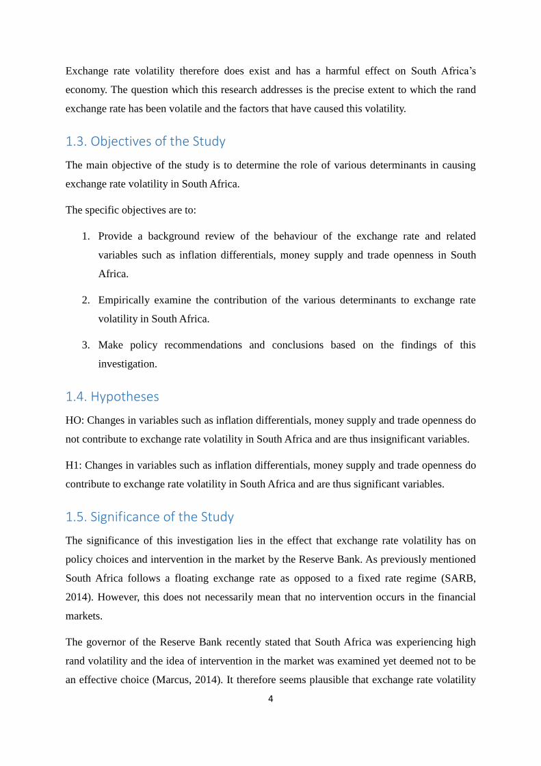
Presidency of the Republic of South Africa, 2006). Figure 2.1 indicates a somewhat

downward trend for South Africa’s REER with volatility around the trend. According to De

Jager (2010) currency depreciation may be accompanied by movements to liberalise and

reduce trade restrictions with the aims of achieving greater trade openness. The sudden

7

openness of the South African economy to the global environment after a lengthy era of

financial restrictions and trade sanctions during the Apartheid era may have affected rand

stability.

Figure 2.1: Real Effective Exchange Rate of South Africa (1994-2014)

Source: SARB, Historical Macroeconomic Time Series Information (KBP5392M)

In the years 1997 and 1998 the East Asian community was faced with a financial crisis: large

capital inflows resulting from increased economic success placed greater demands on

financial organizations, and these important role players were unable to consistently match

these demands (IMF Staff, 1998). Financial regulators and practices that were meant to

protect the financial sector were not prepared for the huge influx of financial flows and the

consequential demands of investors. Due to global interdependence, this downfall of the East

Asian community’s financial sector caused many investors to switch from emerging market

investments to the ‘safer’ currencies of developed nations (Bhundia and Ricci, 2006). Many

emerging markets or developing countries thus would have experienced a fall in foreign

investment.

According to Bhundia and Ricci (2006) the East Asian crisis resulted in a fall in demand for

internationally traded commodities, causing prices of South Africa’s exported goods and

services to decrease which resultantly led to a currency depreciation. As a result of the impact

that the 1998 crisis had on the rand, intervention was required in the form of the SARB,

which decided to “support the Rand by substantial sales of dollars out of the foreign reserves,

as well as intervention in the forward Rand-dollar market” (Matemba 2002: 2). The SARB

8

thus attempted to strengthen the rand through sales of the US dollar, which reduced the

balance of South Africa’s gold and foreign exchange reserves and assisted in meeting a

heightened demand for US currency.

In 2001 the rand once again experienced a downfall in the foreign exchange market, despite

the belief of ‘sound fundamentals’ in the form of low inflation levels and a reasonable current

account balance (Matemba, 2002). It was questionable as to what may have impacted the

rand in such a negative manner in the presence of what appeared to be a thriving economy.

The government appointed the Myburgh Commission with the task of uncovering the cause

of the rand’s demise. The Commission indicated in their final report that the rand

depreciation of 2001 was believed to be due to a number of macroeconomic issues, including

a fall in global economic activity, contagion from Argentinian events, and a deterioration in

the current account balance at the end of 2001 (Bhundia and Gottschalk, 2003).

Matemba (2002) and Bhundia and Ricci (2006) also argue that perhaps it was due to lack of

privatization in this period which resulted in currency depreciation, as plans to privatize

Telkom were put off for extended periods of time and the South African government also

sought out to re-purchase shares held by foreign entities in the airline industry. The failure of

the South African government to timeously begin privatization reforms as promised could

have obstructed the flow of foreign investment. This disruption in foreign investment flows

may have negatively impacted the spot exchange rate.

The years 2002 and 2003 saw a significant improvement in the exchange rate, with the rand

having generally appreciated during this period. Volatility in the early 2000s was therefore

considerable, with the rand initially having undergone a significant depreciation followed by

appreciations in value; this indicates instability. The behavior of the rand in 2002 and 2003

can largely be explained by means of the SARB’s inflation targeting regime. According to

Samson et al (2003) the SARB utilized high interest rates for purposes of disinflation, which

resultantly encouraged capital inflows and led to the strengthening of the rand.

The period 2004 until 2007 was characterized by mild levels of volatility, with slight

fluctuations occurring in 2004 followed with appreciations in 2005 and depreciations in 2006.

During this time period “a steady flow of savings from non-residents into rand-denominated

assets contributed to cheap financing and with a stronger currency made possible the

9

importation of considerable capital equipment, a less costly infrastructure build programme,

and improved welfare for households as imported consumer goods became less costly”

(Kganyago, 2012: 1). The rand thus experienced growth and strengthened against trading

partner currencies. Export revenue would have grown and imported goods and services

became relatively less expensive. However, at the end of 2007 the rand begun to depreciate.

In the years leading up to 2007, mortgage backed securities and collateralized debt

obligations were introduced into the financial markets (Mishkin, 2009). These types of

derivative instruments were allowed to develop within the banking framework present in the

US at the time, and can be stated to have resulted in banking and other financial institutions

to have taken on more risk than in the past. There was a lack of regulation governing the

parties creating such mortgage backed securities, in that they created these instruments and

sold them off without worrying about borrowers’ abilities to repay investors (Miskin, 2009).

The combined effects of risky assets and failure to govern ended in a financial crisis

occurring in the banking industry as debtors began defaulting on payments.

South Africa however did not feel the impact of the global crisis as much as more advanced

economies did. The reasons for this can be attributed to the following four basic

characteristics of the South African financial sector: (1) A sound regulatory framework; (2)

Conservative risk management; (3) Limited exposure to foreign sector assets; and (4) Listing

requirements (Gordhan, 2011). The financial system in South Africa is well regulated, which

led to any possible risks in financial institutions being forecasted and stopped. Risk practices

at commercial banks were also much more conservative than the past, which meant that

derivative trading was far less as compared to more advanced economies. Institutions were

also limited with respect to the level of foreign assets held, which in turn decreased risk from

abroad. And listing requirements have been stringent, ensuring that institutions were highly

transparent to shareholders at the time (Gordhan, 2011).

In 2009 the REER of South Africa improved, and this impacted the level of price

competitiveness of South Africa’s exports (SARB, 2009). With the rand having strengthened

in value, South African goods and services became more expensive in comparison to

products produced in other nations. This caused the rand to lose its competitive value, and

foreign consumers to opt for less expensive, non-South African commodities. This

10

appreciation continued well into 2010, with mild fluctuations around the trend. However, the

rand started to weaken once again in 2011.

From mid-2012 to 2013, the REER of South Africa decreased by 12 percent, which can

greatly be attributed to an increasing deficit, labour unrest and capital outflows (Kumo,

Rielandër and Omilola, 2014). The value of the rand was falling in the midst of ever

increasing national debts, and severe labour disputes resulted in a significant loss of investor

confidence and a large withdrawal of capital. Initially, South Africa only experienced labour

unrest within the platinum mining sector although this soon extended to other mining

industries (Ramutloa, 2013). The issues arising in the mining sector then evolved and began

to influence other sectors, thus providing emerging market investors with enough reason to

withdraw capital from South Africa. This depreciation continued into 2014, although the

impact on consumers was minimised by importers absorbing the added costs (Kumo et al,

2014). Large importers and retailers took on the majority of the increases with little pass

through effects to consumers.

Over the past two decades the rand has experienced significant volatility. There appears to

have been a general downward movement in the value of the rand, but this has been

accompanied by large fluctuations around the trend. These fluctuations have been due to a

number of factors, such as the effects of the East Asian crisis in 1998 and the global financial

crisis of 2008. A number of other underlying indicators have also been mentioned, such as

domestic interest rate movements in the aim of achieving inflationary goals. Rand volatility

could thus be the product of a number of domestic or foreign factors that cause shocks to the

South African economy.

2.3. Government Expenditure

This section shall examine historical changes in national government expenditure for South

Africa and will provide comparisons with respect to exchange rate movements. The relevance

of government spending on the exchange rate has been identified by studies such as Insah and

Chiaraah (2013) and Ajao and Igbekoyi (2013). For this reason, government spending has

been incorporated as a possible determinant of exchange rate volatility in South Africa.

Because of large budgetary deficits in the 1990s, the South African government had to

increase borrowing requirements, which in turn led to large interest payments (Mohr, 2012).

11

These interest payments were so big that they eventually became categorised as a separate

component of government spending. According to the SARB (2013: 8): “National

government expenditure increased at a rate of 9.8 per cent in 1993/94, a considerably lower

rate than the increase of 22.4 per cent in fiscal 1992/93”. Government spending increased at a

lower rate compared to the previous period. Fiscal authorities were shown to have exerted

fiscal restraint in order to reduce the budget deficit of earlier years. In the 1993/94 period,

not all planned expenditure programmes were implemented which aided in reducing this

deficit (SARB, 2013).

Figure 2.2: National Government Spending % Change for South Africa (1994-2014)

Source: SARB, Historical Macroeconomic Time Series Information (KBP4601E, KBP5392Q)

During the 1998/99 period, spending increased overall by a mere 7.6 %, which was

impressive in an economy experiencing low growth at the time (SARB, 2013). One would

expect that in low growth periods spending may have been increased in order to stimulate

demand, but at the time fiscal restraint was considered more prudent. A slight fall in spending

in September 1998 coincided with a large fall in the exchange rate of 15.2%. The exchange

rate thus exhibited significant volatility at the time. The rise in spending that occurred in 1999

is mainly due to non-recurrent payments such as the funding provided to provincial

government departments for debt repayment and Youth Fund transfers aimed at skills

development (SARB, 2013).

12

In the 2002/03 fiscal period government spending started to rise once more, with the focus

shifting away from restricting costs to a more growth oriented approach (SARB, 2013).

Fiscal policy took on a new stance in that increased spending was considered vital in sectors

such as education and health services in order for greater economic growth to occur. This

view continued into the 2003/04 period, with funding being centred on educational resources

rather than government employee benefits (SARB, 2013).

In 2008/09 expenditure increased by 17.4 % and was higher than the budgetary provision:

“Strong growth in national government spending was underpinned by increased voted

expenditure, mainly transfers and subsidies earmarked for social spending and infrastructure

development” (SARB, 2009: 50). Spending was thus still primarily focused on social

components as well as road and rail infrastructure. This rise in government spending was in

line with countercyclical fiscal policy (Lomahoza, Brockerhoff and Frye, 2013).

Countercyclical fiscal policy refers to increased spending during depressed economic

conditions in order to stimulate the economy. In September 2008 and June 2009 large

changes in government spending were associated with appreciations in the REER.

In the 2011/12 fiscal period, the South African governments’ interest expense had increased

from 7.48 percent of the overall budget in the previous fiscal year to 7.88 percent (Lomahoza

et al, 2013). The interest expense component has been continuously increasing since the early

1990s when funding was required. South Africa was devoting a large portion of funds to

interest costs which could have rather been utilised on important socio-economic services.

The National Treasury were employed with the task of identifying measures to ensure

sustainability of public finances in the long run (Gordhan, 2011). This was done to try and

stabilise finances and ensure that interest expenses would not continue to crowd out social

spending.

In 2012/13 national government expenditure grew to R1 trillion, doubling that of 2007/08

(Statistics South Africa, 2014). Government spending thus grew significantly following the

financial crisis. This is in accordance with the countercyclical approach adopted by fiscal

authorities, in that increased spending is needed in order for growth to occur. Spending on

infrastructure is expected to account for R827 billion over the next three years, with the focus

being on Transnet (STANLIB, 2014). In January 2012 when government spending changed

by 21.1% there appears to have been an appreciation in the exchange rate by 5.5%.

13

2.4. Money Supply

This section shall examine the relationship between changes in money supply and exchange

rate movements in South Africa between 1994 and 2014. The importance of money supply as

a possible determinant of exchange rate volatility lies in the effect that money supply has on

price levels. Should domestic money supply rise, price levels will rise and the exchange rate

would be expected to depreciate (Daniels and VanHoose, 2002).

Figure 2.3: Money Supply % Change for South Africa (1994-2014)

Source: SARB, Historical Macroeconomic Time Series Information (KBP5392Q); OECD,

MEI (MEI-ZAF_MABMM301_GPSAQ).

Towards the end of the 1980s and the early 1990s the SARB targeted money supply: “At the

end of each year it announced minimum and maximum growth rates for growth in the money

stock (nominal M3) for the coming year” (Fourie and Burger, 2015: 85). Steps were then

taken to ensure that growth rates remained within the specified levels. However, due to

increased openness of the capital account and financial liberalization money supply targeting

became increasingly difficult (Aziakpono and Wilson, 2010). As financial liberalization and

innovation occurred, it became near impossible to control the growth of money supply.

Due to the trouble experienced in targeting money supply, discussions between the SARB

and National Treasury occurred in 2000 wherein it was decided that an inflation targeting

framework would be adopted, with inflation being allowed to vary between a band of three

14

and six percent (Ricci, 2006). In order to ensure that inflation remains within acceptable

levels, intermediate policy objectives may be set. In the past, intermediate policy objectives

also involved targeting money supply, but in 1998 the SARB decided to switch to targeting

interest rates (Fourie and Burger, 2015). The interest rate that was chosen to be targeted was

the repurchase rate. It may be observed in Figure 2.3 that a small rise in money supply in

June 1995, December 1997 and June 1998 was linked with a fall in the exchange rate, with

the percentage change in 1998 being rather significant.

In the first quarter of 2002 money supply grew significantly, but this growth rate deteriorated

towards the year end; a tightening of monetary policy is partly responsible for this slowdown,

as funds flowed to and from asset markets dependent on the SARBs actions in halting

inflationary pressures and this assisted in reducing M3 growth (SARB, 2002). As the SARB

took steps to reduce inflation in line with the inflation targeting scheme, investors reacted

through influencing the flow of funds to asset markets. The level of growth that did take

place in M3 in the third quarter of 2002 was primarily due to household contributions

(SARB, 2002). Business sector holdings contributions had decreased in comparison to

previous periods.

In the 2003/04 period growth in M3 deteriorated due to the removal of stamp duty on

promissory notes: “Banks then increased their issues of negotiable promissory notes (not

included in M3) at the expense of negotiable certificates of deposits (included in M3), which

reduced the growth rate of M3” (Van der Merwe and Mollentze, 2010: 50). Stamp duties

were still implemented on NCDs which led to this substitution and slowdown in M3 growth.

However, monetary authorities soon corrected this substitution issue through the decision to

incorporate promissory notes into the definition of M3 (Van der Merwe and Mollentze,

2010). This decision meant that any substitution would only lead to a change in the

composition of M3 rather than a change in growth rates. With respect to the exchange rate,

there was a small rise in money supply in December 2003 whilst a decrease in the REER

occurred.

Due to the manifestation of the financial crisis in 2007/08 money supply growth once again

began to deteriorate, and this continued in the year thereafter. M3 growth decreased between

2008 and 2009, partly due to lower household and company income and spending as well as

strict credit conditions (SARB, 2009). Strict credit control meant that the creation of money

15

through the commercial bank lending process was reduced. Between 2007 and 2009 money

supply growth was mainly on a downward trend, with the exchange rate being observed as

having been quite volatile during this time.

Growth in M3 increased between December 2012 and the first quarter of 2013 as a reflection

of small improvements in general economic conditions in South Africa (Bhorat et al, 2013).

This growth in 2013 was mostly due to a rise in household and company income and

spending due to financial market instability (Bhorat et al, 2013). With volatility being

experienced in financial markets individuals preferred money holdings. Money holdings were

seen as a less risky asset in comparison to other financial assets. The REER during this period

appears to have been less volatile.

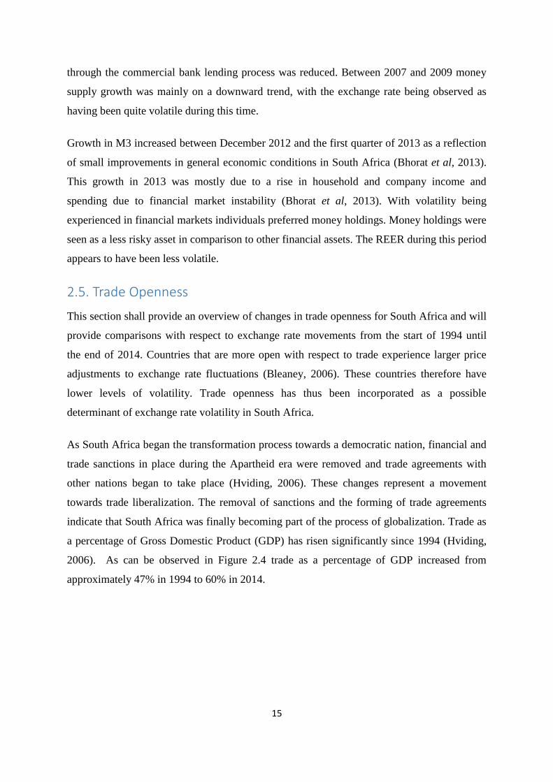
2.5. Trade Openness

This section shall provide an overview of changes in trade openness for South Africa and will

provide comparisons with respect to exchange rate movements from the start of 1994 until

the end of 2014. Countries that are more open with respect to trade experience larger price

adjustments to exchange rate fluctuations (Bleaney, 2006). These countries therefore have

lower levels of volatility. Trade openness has thus been incorporated as a possible

determinant of exchange rate volatility in South Africa.

As South Africa began the transformation process towards a democratic nation, financial and

trade sanctions in place during the Apartheid era were removed and trade agreements with

other nations began to take place (Hviding, 2006). These changes represent a movement

towards trade liberalization. The removal of sanctions and the forming of trade agreements

indicate that South Africa was finally becoming part of the process of globalization. Trade as

a percentage of Gross Domestic Product (GDP) has risen significantly since 1994 (Hviding,

2006). As can be observed in Figure 2.4 trade as a percentage of GDP increased from

approximately 47% in 1994 to 60% in 2014.

16

Figure 2.4: Trade Openness of South Africa (1994-2014)

Source: SARB, Historical Macroeconomic Time Series Information (KBP6006C; KBP6013C;

KBP6014C; KBP5392Q)

In the early 1990s protective measures actually increased, with tariffs rising to approximately

20% in 1993 (Thurlow, 2006). It was only in the latter part of the era after the first

democratic election that liberalization began to occur. In 1994 South Africa “signed the

Marrakech Agreement under the Uruguay Round of the GATT…the deal involved reducing

the number of tariff lines to six, rationalising the twelve thousand commodity lines and

replacement of quantitative restrictions on agriculture by tariff equivalents” (Mabugu and

Chitiga, 2007: 4). The Marrakech Agreement proposed the replacement of quotas on

agricultural products with tariffs, so that there would be no limit on the number of items

imported. The reduction in tariff lines would enable international comparisons. As can be

observed in Figure 2.4, a fall in trade openness in 1997 was accompanied by a more volatile

exchange rate.

In an attempt to achieve greater liberalization, South Africa also became a member of a

number of trade agreements in the post-Apartheid era. In 1994 South Africa became a

member of the Southern African Development Community (SADC) and in 1996 the country

signed a trade protocol with the intention of creating a free trade area for eight years

(Hviding, 2006). The purpose behind the trade protocol was the aim of achieving greater

international competitiveness. In 2000 the United States formed an agreement with South

17

Africa, under which free access was granted to various agricultural commodities (Hviding,

2006). South Africa could now purchase certain products at duty free rates through the

United States.

With the global financial crisis of 2008, global demand decreased and South Africa’s exports

resultantly fell by 21% in the first quarter of 2009 (SARB, 2009). South Africa faced low

demand from trading partners like the US and Japan, which ultimately impacted the level of

trade taking place. According to SARB (2009: 23): “The sharp decline in the volume of

merchandise exports together with only a moderate increase in the price of exported goods

caused the value of exports to recede by 19.4 percent, from R668.2 billion in the fourth

quarter of 2008 to R538.4 billion in the first quarter of 2009”. Due to this fall in the value of

exports, trade as a percentage of GDP also decreased. In 2009 the REER is observed as

having experienced significant fluctuations around the trend.

In 2013 exports increased from R817 to R846 billion whilst imports increased from R852 to

R921 billion (Kumo et al, 2014). The rise in exports was mainly due to the decline in the

value of the rand, which caused South African products to be relatively less expensive in

comparison to those of other countries. In 2014 exports began to fall in the second quarter,

but this reversed before year end primarily due to a rise in manufacturing and agricultural

exports (SARB, 2014). In the beginning of 2014, when this fall in trade openness occurred,

the exchange rate experienced slight volatility.

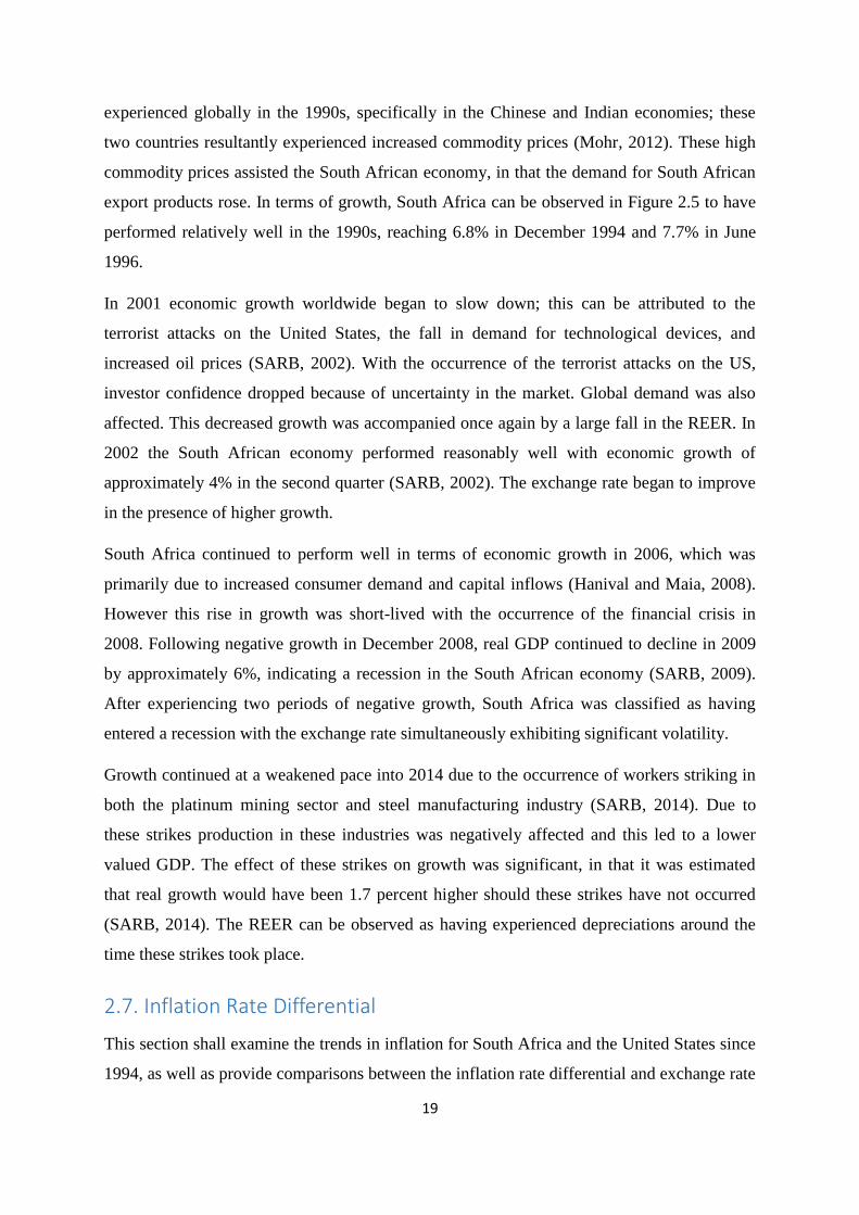
2.6. Economic Growth

This section shall examine historical movements in economic growth for South Africa as well

as provide comparisons with changes in the exchange rate. The relevance of economic

growth on exchange rate volatility has been proven by studies such as Ding (2003) who

identified that during times of increased economic growth, exchange rate volatility decreases.

Good economic performance provides a positive environment for exchange rate stability. For

this reason, economic growth (real GDP) has been included as a possible determinant of

exchange rate volatility in South Africa.

18

Figure 2.5: Real GDP Performance of South Africa (1994-2014)

Source: SARB, Historical Macroeconomic Time Series Information (KBP6006S,

KBP5392Q).

The years 1994 until 2014 may be described as a period during which sustained, moderate

growth was experienced (Mohr, 2012). This is in comparison to the periods preceding the

democratic elections. The most significant contribution to growth since 1994 can thus be

ascribed to “the abolition of financial sanctions and the restoration of free access to the

international capital markets” (Mohr, 2012: 113). After Apartheid, the bans on capital flows

were lifted and finance started to flow to South Africa. This aided in reducing budget deficits

on the balance of payments.

In 1996 South African authorities introduced the Growth, Employment and Redistribution

(GEAR) initiative, the aim of which was to achieve long-term sustained growth, increased

employment rates and to address the issues of unequal income distribution (Department of

Finance, 1996). Since the introduction of GEAR, a number of other growth policy initiatives

have been borne. This includes but is not limited to the Accelerated and Shared Growth

Initiative of South Africa (ASGISA) in 2006, the New Growth Path in 2010 and the National

Development Plan (NDP) in 2013 (Fourie and Burger, 2015).

It appears that in 1998 when a fall in growth was experienced in South Africa, the exchange

rate was quite volatile in that a large percentage change occurred in the form of a

depreciation. But other than the East Asian crisis in 1998, significant growth was

19

experienced globally in the 1990s, specifically in the Chinese and Indian economies; these

two countries resultantly experienced increased commodity prices (Mohr, 2012). These high

commodity prices assisted the South African economy, in that the demand for South African

export products rose. In terms of growth, South Africa can be observed in Figure 2.5 to have

performed relatively well in the 1990s, reaching 6.8% in December 1994 and 7.7% in June

1996.

In 2001 economic growth worldwide began to slow down; this can be attributed to the

terrorist attacks on the United States, the fall in demand for technological devices, and

increased oil prices (SARB, 2002). With the occurrence of the terrorist attacks on the US,

investor confidence dropped because of uncertainty in the market. Global demand was also

affected. This decreased growth was accompanied once again by a large fall in the REER. In

2002 the South African economy performed reasonably well with economic growth of

approximately 4% in the second quarter (SARB, 2002). The exchange rate began to improve

in the presence of higher growth.

South Africa continued to perform well in terms of economic growth in 2006, which was

primarily due to increased consumer demand and capital inflows (Hanival and Maia, 2008).

However this rise in growth was short-lived with the occurrence of the financial crisis in

2008. Following negative growth in December 2008, real GDP continued to decline in 2009

by approximately 6%, indicating a recession in the South African economy (SARB, 2009).

After experiencing two periods of negative growth, South Africa was classified as having

entered a recession with the exchange rate simultaneously exhibiting significant volatility.

Growth continued at a weakened pace into 2014 due to the occurrence of workers striking in

both the platinum mining sector and steel manufacturing industry (SARB, 2014). Due to

these strikes production in these industries was negatively affected and this led to a lower

valued GDP. The effect of these strikes on growth was significant, in that it was estimated

that real growth would have been 1.7 percent higher should these strikes have not occurred

(SARB, 2014). The REER can be observed as having experienced depreciations around the

time these strikes took place.

2.7. Inflation Rate Differential

This section shall examine the trends in inflation for South Africa and the United States since

1994, as well as provide comparisons between the inflation rate differential and exchange rate

20

movements. The use of the US inflation rate is due to the ease of data availability for this

economy. Although the United States may not be the largest trading partner, economic data

for this developed country is readily available. Trends for both the South African and United

States inflation rates may be observed in Figure 2.6.

Figure 2.6: Inflation Rate Performance for the United States and South Africa (1994-2014)

Source: IMF, International Financial Statistics (IFS-I19964__XZFQ, IFS-I11164__XZFQ).

The relevance of the inflation rate differential to this study is the impact that a rise in prices

has on international competitiveness. Should South Africa experience a higher inflation rate

in comparison to the US, a depreciation of the rand is likely to occur (Mohr, 2012). This will

result in further inflationary pressure as import prices rise. Variations in the inflation rate

differential might thus result in exchange rate fluctuations. Figure 2.7 can be used to observe

movements in the inflation rate differential in comparison to fluctuations in the REER.

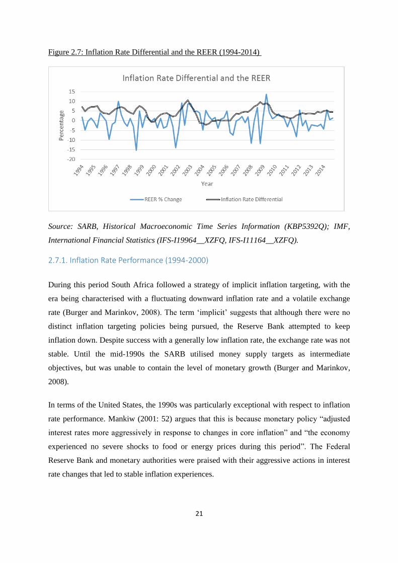
21

Figure 2.7: Inflation Rate Differential and the REER (1994-2014)

Source: SARB, Historical Macroeconomic Time Series Information (KBP5392Q); IMF,

International Financial Statistics (IFS-I19964__XZFQ, IFS-I11164__XZFQ).

2.7.1. Inflation Rate Performance (1994-2000)

During this period South Africa followed a strategy of implicit inflation targeting, with the

era being characterised with a fluctuating downward inflation rate and a volatile exchange

rate (Burger and Marinkov, 2008). The term ‘implicit’ suggests that although there were no

distinct inflation targeting policies being pursued, the Reserve Bank attempted to keep

inflation down. Despite success with a generally low inflation rate, the exchange rate was not

stable. Until the mid-1990s the SARB utilised money supply targets as intermediate

objectives, but was unable to contain the level of monetary growth (Burger and Marinkov,

2008).

In terms of the United States, the 1990s was particularly exceptional with respect to inflation

rate performance. Mankiw (2001: 52) argues that this is because monetary policy “adjusted

interest rates more aggressively in response to changes in core inflation” and “the economy

experienced no severe shocks to food or energy prices during this period”. The Federal

Reserve Bank and monetary authorities were praised with their aggressive actions in interest

rate changes that led to stable inflation experiences.

22

Changes in the inflation differential between 1994 and 2000 can mainly be attributable to

South Africa’s inflation rate changes. Despite a general downward movement in inflation,

South Africa experienced significant fluctuations around this trend whilst the United States

inflation exhibited greater consistency. In South Africa in the early 1990s interest rates were

kept at a minimum to encourage growth, but this came at the expense of higher inflation

(Ricci, 2006). The downward movement in the inflation differential in 1994 was

accompanied by a fall in the REER. Similarly, in both 1996 and 1998 a fall in the inflation

differential was accompanied by a significant depreciation in the exchange rate.


In the year 2002, after discussion with all relevant parties such as the National Treasury and

government officials, the SARB introduced an inflation targeting regime whereby inflation is

allowed to float between three and six percent (Ricci, 2006). Ultimately the goal of the SARB

is to maintain inflation within this band by allowing slight room for movement. Inflation

levels actually exceeded the 6 % ceiling at first introduction, but this can partly be attributed

to the negative after effects that the 2001 bombings in the United States had on trade

(Industrial Development Corporation, 2013). Due to the relevance of the US dollar in trade,

global prices (including South African commodity prices) were affected. The sharp

depreciation of the rand at the time could also be accountable for the rise in prices.

In terms of the United States itself, the effect that the 2001 bombings had on inflation rates

was of a short term nature: “with inflation expectations well-anchored, the Fed has been able

to provide liquidity in response to financial disruptions without causing uncertainty about the

long run goals of policy” (Poole and Wheelock, 2008: 7). The Federal Reserve Bank reacted

correctly by providing necessary funds, whilst managing to maintain the long run

expectations regarding inflation rates.

Despite numerous changes to South Africa’s inflation targeting framework since its

introduction, it has largely been successful with inflation dropping to approximately three

percent in July 2005 (Ricci, 2006). This improvement in inflationary pressures has added to

the perception of financial stability in South Africa. Some of the amendments to the inflation

targeting regime include an explanation clause and increases in the number of Monetary

Policy Committee meetings that take place (Nowak, 2006). The explanation clause by

definition merely means that monetary authorities are required to provide reasons for

23

inflation rate changes. Increasing the frequency of committee meetings allows for more open

communication.

From 2001 up until 2005 the inflation differential generally increased. This is once again

mainly attributable to the changes in South Africa’s inflation rate. Although the inflation rate

in the United States increased in 2001, this rise was slight. The combination of the effects of

the 2001 bombings in the United States, as well as the findings made by the Myburgh

Commission for instability in the exchange rate, provide a basis for explaining the high

inflation rate levels in South Africa. A slight fall in the differential in 2001 was matched with

a large descent in the exchange rate. However, when the differential began to increase once

more the exchange rate followed suit. Similarly when the differential fell in 2002 this was

matched by a general downward movement in the REER.


According to Hanival and Maia (2008: 19): “Inflationary pressures started to come to the fore

during 2006 as the low interest rate environment resulted in a massive uptake of credit,

boosting consumer demand to record levels”. The initial boom in the South African economy

during 2006 caused prices to rise, as producers were unprepared for such high demand and

shortages were experienced. This higher inflation continued into 2007 and 2008: “the global

commodity boom (including the hike in oil and food prices), aggravated by a weaker rand,

filtered through producer and consumer prices, leading to the inflation target ceiling being

overshot” (Hanival and Maia, 2008: 19). Both producers and consumers were forced to pay

higher prices for intermediate and end products, and ultimately the 3-6 % inflation band was

exceeded.

The 2007/08 global financial crisis and heightened oil and commodity prices led to inflation

in South Africa reaching 9.9% in 2008, with inflation thereafter continuing to average around

5.5% up until 2012 (Industrial Development Corporation, 2013). Despite the best efforts of

SARB to maintain inflation at lower levels, the financial crisis had a long term effect on price

levels in South Africa. Between 2009 and 2012, the SARB were however still able to

maintain figures below the 6 % ceiling.

In the United States there was actually concern regarding deflation in 2008, with inflation

falling from approximately 2% down to 1% (Neely, 2010). This fall in the general price level

24

could be seen as a deterrent to economic growth. As can be observed in Figure 2.6, there is a

distinct decrease in the United States inflation rate which started in 2008 and continued well

into 2009. According to Neely (2010: 1) “Economists debate the extent to which deflation

directly harms the economy or is merely a symptom of a negative shock, such as a financial

crisis, that reduces economic activity… regardless, deflation can be harmful”. Deflation could

have appeared as a symptom of the financial crisis or was a sign of a greater underlying

problem in the United States. Either way there are negative consequences attached with

deflation and so it was deemed unwelcome by monetary authorities.

Due to the financial crisis, the inflation differential between 2006 and 2010 was of an upward

trend. This is due to both the rise in inflation for SA and the US at the height of the crisis in

2008, and the resulting deflation experienced in the United States thereafter. In terms of the

exchange rate, when the differential began to fall in 2009 the REER also exhibited a

downward movement. Preceding this, it is not possible to observe a systematic relationship

between the two variables in the years covering 2006 until 2010.


In 2011 inflation reached a rate of more than 3% in the United States, but by mid-2012 had

once again deteriorated to well below 2% which sparked concerns regarding deflation. Sivy

(2012) argues that the problem associates with the fact that consumers may still be unwilling

to spend after the global financial crisis. With consumers spending less, there was little to

stimulate a rise in prices and a resultant rise in the overall inflation rate. As a result, deflation

occurred. In 2013 and 2014 similar incidents were experienced, with inflation decreasing to

1.2% in 2013, which was below the Federal Reserve’s 2% target (STANLIB, 2014). The

Federal Reserve aim to keep inflation at a standard of approximately 2% and thus although

well controlled, the 1.2 % inflation rate could have been an indication of low levels of

consumption expenditure.

With respect to South Africa, the inflation rate began to increase in 2014, and this was mainly

due to South Africa’s weaker exchange rate under which “the Monetary Policy Committee of

the South African Reserve Bank decided to raise interest rates…to anchor inflation

expectations” at the expense of growth (Industrial Development Corporation, 2014: 2). By

anchoring expectations due to inflationary pressures, the SARB run the risk that economic

performance and growth may be low for the coming period.

25

The inflation rate differential between South Africa and the United States from 2011 until

2014 experienced less movement in that no significant economic shocks affected price levels.

Volatility in the exchange rate may therefore be better explained by examining the effect of

other variables during this time period.

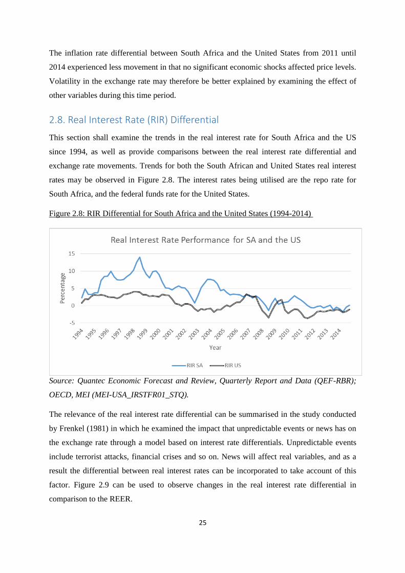
2.8. Real Interest Rate (RIR) Differential

This section shall examine the trends in the real interest rate for South Africa and the US

since 1994, as well as provide comparisons between the real interest rate differential and

exchange rate movements. Trends for both the South African and United States real interest

rates may be observed in Figure 2.8. The interest rates being utilised are the repo rate for

South Africa, and the federal funds rate for the United States.

Figure 2.8: RIR Differential for South Africa and the United States (1994-2014)

Source: Quantec Economic Forecast and Review, Quarterly Report and Data (QEF-RBR);

OECD, MEI (MEI-USA_IRSTFR01_STQ).

The relevance of the real interest rate differential can be summarised in the study conducted

by Frenkel (1981) in which he examined the impact that unpredictable events or news has on

the exchange rate through a model based on interest rate differentials. Unpredictable events

include terrorist attacks, financial crises and so on. News will affect real variables, and as a

result the differential between real interest rates can be incorporated to take account of this

factor. Figure 2.9 can be used to observe changes in the real interest rate differential in

comparison to the REER.

26

Figure 2.9: RIR Differential and the REER (1994-2014)

Source: SARB, Historical Macroeconomic Time Series Information (KBP5392Q);

QUANTEC (QEF-RBR); OECD, MEI (MEI-USA_IRSTFR01_STQ).

2.8.1. Performance of Real Interest Rate (1994-2000)

Based on comparative analyses conducted by Kahn and Farrell (2002) the average real

interest rates for South Africa up until the year 1994 were not significantly different from

those of other nations. This suggests that the RIR differential between South Africa and other

countries up until this point in time was small in nature. Some possible reasons for this

change in differentials in the 1990s are: “other countries liberalised at earlier times…the 1996

rand crisis which resulted in tighter monetary policy…the tight monetary policy reaction to

the sharp depreciation of the rand following the Asian and Russian crises in 1998” (Kahn and

Farrell, 2002: 15). Other countries across the globe liberalised interest rates before South

Africa, thus allowing them to adjust to market forces. Monetary policy reactions in both 1996

and 1998 also restricted interest rates in South Africa.

In 1999 the SARB decreased the repo rate, causing short term market interest rates to fall

(Kahn and Farrell, 2002). By reducing the repo rate the central bank affected the lending

abilities of commercial banks. These banks in turn adjusted their lending rates in line with the

repo rate. South Africa’s real interest rate appears to be both higher and more volatile than

the United States during this time period.

27

With respect to the US, the Federal Reserve adjusted reserve requirements of banks in the

1990s which led to slight volatility in the federal funds rate as commercial banks attempted to

adjust reserve balances (Hilton, 2005). As commercial banks altered their positions at the

central bank, changes in their positions at the Reserve led to these banks being either

overdrawn or holding excess reserves. This in turn impacted interest rates and caused

fluctuations in the federal funds rate.

Movements in the differential over this time period were largely due to fluctuations in South

Africa’s repo rate as volatility in the federal funds rate was not as severe. In the years 1996

and 1998 this differential is particularly high. The rise in the differential in both these years is

accompanied by a large declination in the exchange rate. And when the real interest rate

differential reached a low point in 1995 and 1997 the exchange rate is shown to have

improved.


Upon the occurrence of the 2001 terrorist attacks the Federal Reserve decreased the federal

funds rate from 3% to approximately 2.5% in order to prevent the United States from

dropping into a recession (Money CNN, 2001). Due to uncertainty regarding economic

conditions both business and household expenditure had deteriorated. In an effort to stimulate

spending the central bank reduced the federal funds rate which in turn affected other market

rates. The effect of a decrease in rates at first led to United States stock prices falling,

although this fall in prices was of a short term nature (Money CNN, 2001). Potential

investors were initially concerned regarding the country’s economic well-being.

The 2001 bombings affected South Africa’s real interest rate only slightly through the change

that occurred in inflation. In 2002 real interest rates decreased but this was mainly due to the

amendments in Monetary Policy with respect to the introduction of an inflation targeting

regime (Industrial Development Corporation, 2013). Initially inflation breached the 6%

bandwidth set out by the SARB. Due to this rise in inflation, real interest rates decreased at

the time.

Although the US real interest rate exhibits a slight downward trend during this time, changes

in South Africa’s real interest rate were mainly responsible for fluctuations in the differential.

More specifically, the rise in the differential in 2002 occurred due to Monetary Policy

28

changes in South Africa. At this time, the rise in the differential was partnered with a fall in

the exchange rate.


Moving from the financial crisis of 2008 and into 2009, the South African Monetary Policy

Committee opted to gradually decrease the repo rate by approximately 450 basis points in

accordance with the decision to undertake monetary policy easing (SARB, 2009). By

reducing the repo rate other market interest rates also declined, enabling borrowing to take

place at lower rates and thus stimulating consumer and business spending. But Kyangago

(2015) notes that low rates are unsustainable in the long run in that savers receive negative

returns. National savings will be negatively affected should real interest rates continue to

remain at low levels.

In the United States, monetary authorities took more drastic action following the 2008

financial crisis by decreasing interest rates to near-zero values (McGregor, 2012). This was in

reaction to the shock of the financial crisis to the economy in an attempt to stimulate

spending. According to McGregor (2012: 4): “the proponents of zero rates argue that they

stabilise the economy, that they relieve the pressure on highly indebted consumers and, by

making the cost of capital cheaper, encourage investment”. Zero interest rates are therefore

seen as beneficial by allowing consumers relief from high debt costs, and also by allowing

potential investors the opportunity to obtain capital at relatively low prices. But once again

the problem of negative returns to savers becomes an issue.

The real interest rate differential fluctuated only slightly between 2005 and 2010. The reason

for this lies in that both South Africa and the United States reduced rates following the

occurrence of the financial crisis. With respect to inflation rates, South Africa experienced

higher inflation in comparison to the United States. This also brought South Africa’s real

interest rate closer in value to that of the United States. A slight fall in the differential in 2009

was accompanied by an increase in the exchange rate, although there seems to be no other

significant relationship between the two variables during this time.


According to McGregor (2012: 6): “Since mid-2011 the base interest rate set by the South

African Reserve Bank has also been lower than the inflation rate” and real rates were thus

29

negative over this period of time. Looking at the broader picture, South Africa had been

fortunate with respect to achieving mainly positive real interest rate values for a number of

years in comparison to more developed nations. In 2014 the SARB raised the repo rate by 75

basis points, but real interest rates still remained negative (Maswanganyi, 2014).

The trend of zero or negative real interest rates continued for the United States throughout

this time period. It appears that the trend with respect to these rates is to maintain low values

until the economy experiences higher growth. However, the long term impact of zero rates,

specifically on those consumers dependent on interest income, needs to be carefully

considered.

The real interest rate differential revolved near zero between 2011 and 2014, in that South

Africa’s real interest rate was not significantly different from that of the United States.

Around this time there were also no significant shocks to the South African economy, and the

REER experienced mild volatility in comparison to that of previous years.

2.9. Conclusion

This chapter supplied a backdrop to the study by analysing developments in the exchange rate

and through providing an overview of related variables. After examining movements in the

REER of South Africa, it may be stated that the rand experienced significant levels of

volatility between 1994 and 2014. This volatility is particularly pronounced during times of

crises, such as the East Asian Crisis of 1998, the terrorist attacks in the United States in 2001

and the global financial crisis in 2008. Increases in government spending were observed as

being accompanied by appreciations of the REER, with the exchange rate seeming to be less

volatile at the time these expenditures occurred. Money supply increases were accompanied

primarily by depreciations in the exchange rate. During periods of lower trade openness and

decreased economic growth the REER was also observed as being more volatile. And a rise

in either the inflation or interest rate differentials resulted in greater volatility. Chapter three

shall provide a background to both theoretical and empirical literature on the exchange rate

and related variables.

30

Chapter Three

Literature Review

3.1. Introduction

The purpose of this specific chapter is to provide an overview of both theoretical and

empirical literature obtained that is relevant to the research issue at hand. Definitions

regarding exchange rates are discussed in section 3.2, and can be classified into two

categories: nominal and real exchange rates. These definitions are further expanded to

incorporate effective rates. Section 3.3 presents exchange rate theories such as the purchasing

power parity theories, the monetary model, the portfolio balance approach and the balance of

payments theory. The purpose of reviewing these traditional theories is that they will assist in

specifying a model for this investigation. Each theory provides prospective factors that could

impact exchange rate volatility for South Africa. In terms of empirical literature, studies

conducted by researchers examining determinants of exchange rate volatility are examined in

section 3.4. The chapter concludes with an assessment of all theoretical and empirical

literature obtained in section 3.5.

3.2. Exchange Rate Definitions

3.2.1. Nominal Exchange Rate

The nominal exchange rate is “merely the price of one currency in terms of another with no

reference made to what this means in terms of purchasing power of goods/services” (Pilbeam,

1998: 11). This rate is the rate that is widely used and stated on a daily basis. For example,

the rand per dollar can be expressed as R10.73. What this shows is that one dollar when

converted to the rand is equal to R10.73.

The nominal exchange rate is thus the prevailing bilateral spot rate in the foreign exchange

market, and arises through the interaction of demand for and supply of foreign currency

(Appleyard, Field and Cobb, 2010). This rate is therefore market determined, in that the

forces of demand and supply for any given currency are free to establish a general

equilibrium price and quantity. Reasons for demanding foreign currency could for example

arise through domestic consumers purchasing foreign goods and services, whilst suppliers

consist of foreign individuals who purchase domestically produced goods and services.

31

The problem with the nominal exchange rate however is that because it does not take into

account price differences between countries, it gives no indication of international

competitiveness (Pilbeam, 1998). The nominal exchange rate thus does not provide any

indication of the level of foreign goods/services that could be purchased with domestic

goods/services.

This rate is also limited in that “it does not provide information about what the spot rate

should be, given the nature and structure of the two countries” and “it does not provide any

information on the change in overall strength of the domestic currency with respect to all of

the home country’s trading partners” (Appleyard, Field, and Cobb, 2010: 482). The nominal

exchange rate thus does not give any indication as to what the prevailing rate should be, but

only indicates what the actual exchange rate is at any particular time. It is also only a measure

of the going rate between two countries, rather than an evaluation of a domestic currency

versus multiple foreign currencies.

3.2.2. Nominal Effective Exchange Rate

The nominal effective exchange rate (NEER) is explained as “a trade weighted index of the

average value of a country's currency” (Appleyard, Field and Cobb, 2010: 483). What this

shows is that instead of for example calculating the rand per dollar exchange rate, one can

compute an index in which the rand is compared to a number of currencies. This index is also

trade weighted, which means that the weights of each currency included within the basket

depends on the level of trade that each conducts with South Africa. The method to calculating

a trade weighted NEER can be shown via the following formula:

(3.1)

Where,

is the nominal effective exchange rate for period 1,

is the nominal exchange rate in foreign currencies per unit of local currency in period 1,

is the bilateral trade weights assigned to each currency (j = 1…..m), and

Π is a symbol to indicate the products of

(Weerasekera, 1992).

32

As can be observed by equation 3.1, the NEER index shows if a specific currency is either

appreciating or depreciating against a particular basket of trade weighted currencies. The

following calculation is used in calculating trade weightings:

(3.2)

Where,

are the shares of each partner country in total trade of the home country in the base year


Measurement problems that may be experienced with respect to computing an NEER index

are that decisions have to be made regarding which currencies are relevant, whether import or

export flows should be used in calculations, and the choice of a base year (Daniels and

VanHoose, 2002). The answers to these questions would all depend on each individual

situation. In most cases, trading partners that account for the majority of trade flows with the

domestic country should be considered in calculations. Trade data regarding import or export

flows (or both) would then need to be examined in order to determine whom these larger

trading partners are with respect to the home country.

It can be concluded by saying that the major benefit of creating an NEER index is that it is a

multilateral rate which indicates the overall strength of the rand against a number of

currencies instead of just one. However, this index still does not account for purchasing

power (Van der Merwe and Mollentze, 2010). Equation 3.1 indicates that no reference is

made to price indexes or inflation within the calculation of the NEER.

3.2.3. Real Exchange Rate

The real exchange rate is a bilateral rate that “adjusts the nominal exchange rate for changes

in nations' price levels and thereby measures the purchasing power of domestic goods and

services in exchange for foreign goods and services” (Daniels and VanHoose, 2002: 42). The

real exchange rate thus overcomes the main weakness associated with nominal exchange

rates, by taking into account inflation differentials between countries. This approach of

adjustment arises from the well-known purchasing power parity theories, which are explained

in section 3.3.1 below. This rate is calculated as follows:

RERppp = E x (PFC/PDC) (3.3)

33

Where,

RER is the real exchange rate as defined by purchasing power parity theories,

E is the domestic currency per unit of foreign currency,

PFC is the foreign country price level/index, and

PDC is the domestic country price level/index

(Solnik and McLeavey, 2004).

Equation 3.3 shows that the real exchange rate is a bilateral exchange rate which is

determined by multiplying the nominal exchange rate with a price index ratio. There are a

variety of price indexes available, which brings about the question of which exact index

should be used as a deflator. The overall objective or purpose of the study will be a deciding

factor in the choice of the price index, as well as the availability of accurate data on these

various indices.

The consumer price index (CPI) and world price index (WPI) have numerous limitations:

they incorporate a large proportion of non-traded items; countries base their indexes on

different baskets; and these indexes include factors that differ across borders such as price

controls (Terra and Abreu, 2005). Non-tradable items are those goods which are not traded on

an international basis. Services are a good example, in that the buyer and seller may need to

be situated in the same location. In computing CPI’s and WPI’s various countries may also

incorporate different baskets into calculations. The reason for this could for example be due

to differing consumption patterns across borders.

Unit labour costs (ULC) and GDP deflators are also considered price indexes, but ULC

measures do not incorporate other factors of production into calculations and labour is

considered immobile, whilst GDP deflators incorporate price changes in non-traded goods

and services (Lafrance, Osakwe and St-Amant, 1998). Labour represents only one of the four

factors of production, rendering this measure slightly biased by not taking into account

important variables such as capital. And GDP deflators face the same issue as CPI’s and

WPI’s in that non-traded items are included.

Based on the above, despite the number of limitations faced by the CPI, this should be the

desired price index. The reason for this choice lies in the ease of data availability of CPI’s for

34

a number of countries (Lafrance, Osakwe and St-Amant, 1998). The main problem faced with

the other price indexes is that not all countries provide adequate data on these indexes.

3.2.4. Real Effective Exchange Rate

The real effective exchange rate (REER) can be defined as “a trade weighted exchange rate

based on real exchange rates instead of on nominal rates” (Appleyard, Field and Cobb, 2010:

484). This is similar to a NEER in that a multilateral index is created based on the level of

trade each country conducts with the domestic country, except that this index is based on the

use of real exchange rates in place of nominal ones. The difference means that this index does

take into account purchasing power (Appleyard, Field and Cobb, 2010). The REER can be

calculated in the following manner:

(3.4)

Where,

is the real effective exchange rate as defined by purchasing power parity theories,

is the nominal exchange rate in foreign currencies per unit of local currency in period 1,

is the bilateral trade weights assigned to each currency (j = 1…..m),

Π is a symbol to indicate the products of , and

is the ratio of the home country’s consumer price index ( ) to foreign country’s

consumer price indices ( )


Equation 3.4 highlights the main advantage of using an REER index as compared to an

NEER index, in that price differences are taken into account. An in-depth discussion has

already been conducted regarding the appropriate price index to be chosen for this study, and

the result was that the CPI was the most commonly used due to international data availability

(Lafrance, Osakwe and St-Amant, 1998). Trade weighting for the REER index is calculated

in much the same way as an NEER index, in that equation 3.2 is utilised.

35

Lastly, it must be stated that it is common knowledge that countries conduct trade with a

number of countries, thus there is the importance of creating an effective exchange rate (or

multilateral exchange rate) as opposed to examining a single nominal or real exchange rate.

3.3. Theoretical Literature Review

3.3.1. Purchasing Power Parity Theories

3.3.1.1. Absolute Purchasing Power Parity Theory

The absolute purchasing power parity theory holds the notion of the law of one price, in that

“identical products should sell for the same price after conversion into a common currency as

a result of the process of arbitrage” (Van der Merwe and Mollentze, 2010: 126). Thus a

common product to two or more countries should cost consumers the same amount after

currency conversions have been completed. The thought behind arbitrage is that the exchange

rate itself should adjust to ensure goods and service prices remain constant across

international borders (Solnik and McLeavey, 2004). If for example a product were to be more

expensive in China than Japan, individuals would try to take advantage of the price

differential between the two countries in order to profit. Consumers would demand more of

the product from Japan and less from China, until eventually prices in China would fall due

to decreased demand and prices in Japan would rise due to increased demand. This process

would lead to the exchange rate between those countries adjusting until prices equilibrate.

The absolute purchasing power parity theory goes on to stipulate that “the exchange rate

should be equal to the ratio of the average price levels in the two economies” (Solnik and

McLeavey, 2004: 46). Thus it builds on the law of one price, in order to find a common

equation that illustrates the determination of an equilibrium exchange rate through using

average price levels. This is demonstrated in the following equation:

E = P/P* (3.5)

Where:

E is the equilibrium exchange rate,

P is the price level in country A, and

P* is the price level in country B

(Van der Merwe and Mollentze, 2010).

36

It must also be realized that absolute purchasing power parity takes into account a weighted

average of a number of goods and services, rather than focusing on the price associated with

a particular good or service (Solnik and McLeavey, 2004). Thus, a ‘basket’ containing similar

homogenous goods and services between two countries should have the same price when

denominated in a common currency. This alleviates the problem of goods in different

countries not being completely identical, so that the theory still appears relevant despite

products being slightly different amongst countries.

Certain issues or weaknesses that have risen with this particular theory cannot however be

ignored. One shortcoming that affects the relevance of the absolute model is the presence of

factors such as tariffs and transportation expenses, of which this model makes no

consideration for (Pilbeam, 1998). One cannot deny that such factors will be present,

particularly with international dealings. Another fault lies in the fact that “there are many

non-traded goods included in the price index of countries that cannot be equated with

international trade” (Van der Merwe and Mollentze, 2010: 126). For example, non-traded

goods could include the cost of visiting a dental practitioner. If such a service is slightly

cheaper in South Africa as compared to China, it is unrealistic to assume that one would

make the journey all the way to China due to the cheaper price.

3.3.1.2. Relative Purchasing Power Parity Theory

This version of purchasing power parity explains how “the appreciation or depreciation of a

currency is given by the difference between the two nations inflation rates” (Daniels and

VanHoose, 2002: 63). The relative purchasing power parity theory is of the view that the

exchange rate between two countries can be explained by inflation differentials, and the

equilibrium exchange rate should adjust to offset these inflation differences. This theory can

be demonstrated by taking into account relative price changes:

E = θP/P* (3.6)

Where,

θ represents a constant reflecting the obstacles to trade

(Dornbusch, 1985).

37

With θ being held constant, the following then holds true as a reflection of the relative

purchasing power parity theory after utilizing logs of the absolute version and differentiating:

ΔE = π – π* (3.7)

Where,

ΔE is a proportionate change in the exchange rate,

π is the inflation rate in country A, and

π* is the inflation rate in country B

(Van der Merwe and Mollentze, 2010).

The relative model is thus a weaker variety of the absolute one, as it highlights the relevance

of changes in prices as compared to absolute prices (Daniels and VanHoose, 2002). By

loosening the definition of purchasing power parity, this latter model overcomes some of the

weakness associated with the absolute model by not focusing on absolute flows but rather

highlighting the importance of the changes in these flows.

Despite this advantage, the relative purchasing power parity theory still presents some major

limitations. Both the absolute and relative models are unable to address financial flows or

money stock changes (Daniels and VanHoose, 2002). These theories thus examine only the

changes in exchange rates that occur as a result of international dealings of goods and

services. It seems inadequate to make no reference to financial flows and money stock

changes considering the overall relative importance of these items in recent years.

A second issue that must be noted is statistical problems, in that countries may associate

different weightings towards different product categories in computing price indexes

(Pilbeam, 1998). This makes it difficult in comparing baskets of goods and services that are

similar. This statistical problem becomes a greater issue in comparing first and third world

countries. Consumers in first world countries are likely to attach greater importance to higher,

more durable quality goods and services whilst consumers in third world countries find

greater significance in basic staple items.

3.3.2. The Monetary Models

There are three main monetary models that often appear in traditional literature, which are all

common in that “the supply and demand for money are the key determinants of exchange rate

38

determination” and “they assume that domestic and foreign bonds are equally risky so that

their expected rates of return are equalized” (Pilbeam, 1998:164). However, this is as far as

the similarities between these models extends. Various differences arise that distinguishes

each from the next, as shall now be discussed.

3.3.2.1. The Flexible Price Monetary Model

The flexible price monetary model for computing a floating exchange rate assumes not only

that prices are flexible, and that domestic and foreign bonds are perfect substitutes, but that

the concept of purchasing power parity holds in the long term (Södersten and Reed, 1994).

Assuming prices are flexible can be extended to say that full employment is incorporated into

the model, and that the exchange rate adjusts automatically to changes in the economy rather

than through government intervention. The concept of purchasing power parity holding in the

long term makes reference to the law of one price and homogenous items costing the same

amount after a common currency conversion.

The flexible price monetary model builds on the Cambridge equations and equilibrium

conditions for money supply and money demand:

Ms = m (D + F) (3.8)

Md = kPy (3.9)

Equilibrium condition occurring where Ms = Md (3.10)

Where,

Ms is money supply,

m is the money multiplier,

D is the domestic component of the monetary base,

F shows the foreign reserve component of the monetary base,

Md is money demand,

k is the desired ratio of nominal money balances to nominal national income,

P is the price level, and

y is real national income

(Salvatore, 2007).

39

Equations 3.8 and 3.9 illustrate the various components that constitute a nations demand for

and supply of money. As shown by equation 3.10, equilibrium occurs when a nation’s

demand for money equals a nation’s supply of money. Based on the above, the following

equations hold true for a two country model, constituting of country A and country B:

(3.11)

(3.12)

Now the absolute purchasing power parity condition E = P/P* can be substituted into the

equilibrium condition for country A, such that:

(3.13)

By incorporating the equilibrium condition, one can now solve for the exchange rate S:

So that (3.14)

(Daniels and VanHoose, 2002).

A given increase in domestic money supply, due to extended domestic credit, will result in

prices to increase and the domestic currency to depreciate (Daniels and VanHoose, 2002). In

essence, when domestic money supply increases and begins to exceed domestic money

demand, consumers are likely to induce greater expenditure, particularly on foreign products.

As this occurs, so will the local currency begin to depreciate in value until the point that

domestic money supply once again equilibrates to domestic money demand.

To state this occurrence in a general perspective, one could say that a country experiencing

higher inflationary pressures compared to other countries, will find the exchange rate

increasing (and local currency depreciates) (Salvatore, 2007). And thus it can also be said for

the reverse that a country experiencing lower inflationary pressures compared to other

countries may find the exchange rate to be decreasing (and local currency appreciating).

With respect to real domestic income, a growth in income will lead to domestic prices falling

and an appreciation of the domestic currency in order to maintain purchasing power parity

40

(Du Plessis, 1998). At the same time therefore a given decrease in real domestic income will

lead to domestic prices rising and a depreciation of domestic currency.

And lastly, a rise in domestic interest rates will cause domestic money demand to drop, and

the domestic currency to depreciate (Pilbeam, 1998). A fall in domestic interest rates will thus

result in domestic money demand to rise and the domestic currency to appreciate.

This model has shortcomings with respect to the belief that purchasing power parity holds in

the long term. The reason for this is due to the fact that the theories surrounding purchasing

power parity have not performed all that well empirically, thus resulting in the flexible price

monetary model to also have shown poor results in historical testing (Pilbeam, 1998).

However, this model is important in that it first introduced the concept of the necessity for

including money stock within exchange rate determination.

3.3.2.2. The Dornbusch Sticky Price Monetary Model

The Dornbusch sticky price monetary model makes reference to the phenomenon of

exchange rate overshooting, as it assumes that both wages and the prices of goods are ‘sticky’

in the short run but that exchange rates adjust immediately to changes in the market

(Södersten and Reed, 1994). Prices of goods or services and the price of labour is relatively

fixed in the short term. When it comes to the wage market in particular, a lot of resistance

will be faced against downward movements in workers’ wages. At the same time exchange

rates are not fixed and freely react to economic shocks.

Exchange rate overshooting can now be explained as how “prices in markets that adjust

relatively quickly to some disturbance may have to overreact (overshoot) in the short term to

compensate for the lack of (or too limited) reaction of prices in markets that adjust more

slowly” (Du Plessis, 1998: 262). In this instance, exchange rate overshooting occurs because

exchange rates overreact in the short term to make up for slow adjustments in the goods

market and labour market. It must be stated here that purchasing power parity thus only

holds in the long term, and does not necessarily hold in the short term. Deviations in

purchasing power parity in the short term can be experienced due to this phenomenon of

exchange rate overshooting occurring.

Another assumption that forms part of the Dornbusch sticky price monetary model is that

uncovered interest rate parity holds at all times, meaning that “if the domestic interest rate is

lower than the foreign interest rate then there needs to be an equivalent expected rate of

41

appreciation of the domestic currency to compensate for the lower domestic interest rate”

(Pilbeam, 1998: 168). Should the local interest rate be lower than foreign rates, local currency

needs to appreciate in order to maintain foreign investment levels. If this does not happen,

then investors will seek to utilize their funds elsewhere to earn greater returns.

How the overall model itself works can now be discussed using a simple example. Assume a

shock such as an increase in domestic money supply. Due to sticky prices in the goods and

labour market, there is now an excess of real domestic money supply. Individual consumers

would only wish to hold onto this excess supply of money should the domestic interest rate

drop (Södersten and Reed, 1994). As stated by the rule of uncovered interest rate parity, as

the domestic interest rate falls and becomes lower than that of the foreign interest rate, the

domestic currency will have to undergo an appreciation. The exchange rate will then have to

depreciate and overshoot the long term equilibrium level in order for an expected

appreciation of the domestic currency to occur that will offset the lower domestic interest

rates (Du Plessis, 1998). In the long run, the markets wherein prices are sticky will gradually

begin to adjust and return the exchange rate back to the normal equilibrium level where

purchasing power parity holds.

The Dornbusch model has been credited with a number of benefits, in that it explicitly makes

reference to returns on portfolios influencing exchange rates and it assists in explaining as to

why exchange rates can be more volatile than actual determinants (Pilbeam, 1998). In terms

of returns on portfolios, this model discusses as to how exchange rates are impacted by

investors seeking to equate their expected yields or returns on worldwide investments. With

respect to volatility, the earlier example in explaining this model made reference as to how a

determinant such as money supply when increased resulted in an even greater depreciation in

the exchange rate.

However, despite these accreditations, there is one major fault of the Dornbusch sticky price

monetary model. This theory makes no reference to specifically incorporate inflation

expectations, despite empirical evidence supporting the importance of such inflation changes

in the past having significantly contributed to exchange rate determination (Pilbeam, 1998).

As a result, further expansion into monetary theories has been conducted.

42

3.3.2.3. The Frankel Real Interest Rate Differential Model

The real interest rate differential model was brought about as an extension of monetary theory

that takes into account factors of importance from both the flexible price monetary model and

the Dornbusch sticky price monetary model. According to Frankel’s theory, the long run

exchange rate is computed in the same way as the flexible price model, whilst the short run

exchange rate on the other hand is altered in order to take into account the importance of real

interest rate differentials (Pilbeam, 1998). Thus in the long run all assumptions remain the

same as that of the flexible price model, whilst in the short run deviations from purchasing

power parity are allowed for due to sticky prices. The following equation can be used to

indicate the determination of the short run exchange rate:

S = (m – m*) – ƞ (y – y*) + σ (Pe – Pe*) – 1/ɵ [(r – Pe) – (r* - Pe*)] (3.15)

Where,

S is the short run exchange rate,

(m – m*) is the relative supply of money for Country A and Country B,

ƞ (y – y*) + σ (Pe – Pe*) is the relative demand for money for Country A and Country B, and

1/ɵ [(r – Pe) – (r* - Pe*)] is the real interest rate differential between Country A and Country

B

(Pilbeam, 1998).

According to equation 3.15, should the real local interest rate fall below the real foreign

interest rate, the real exchange rate would be undervalued in comparison to the normal

equilibrium level, such that domestic currency would be expected to appreciate to account for

this difference in valuation (Pilbeam, 1998). Therefore, in general terms, should there be a

difference in the real interest rate between two or more countries, the real exchange rate

should be expected to differ from the normal equilibrium level.

Despite the developments in monetary theories, these models still hold true to some main

criticisms. One limitation is that these models discuss changes in an exchange rate being

dependent on money demand and supply, but ignore other factors such as the holding of

assets other than money (Van der Merwe and Mollentze, 2010). This approach does not take

into account that individuals have other options in which to hold their wealth.

43

3.3.3. The Balance of Payments Approaches

3.3.3.1 Elasticities Approach

The elasticities approach is a microeconomic theory that focuses on exchange rate

determination and the balance of payments being impacted by changes in prices and the

trading of goods and services (Du Plessis, 1998). This approach focuses on the effect that

changes in trade between countries has on alleviating or improving a specific nation’s balance

of payments deficit or surplus. In terms of the concept of elasticity, this is a measure of how

responsive a change in quantity is to a change in price, with low elasticity indicating a

significant response and high elasticity indicating a minimal response (Van der Merwe and

Mollentze, 2010). For example, low elasticity could show a huge change in the volume of

imports and exports to a change in price whilst high elasticity would show a small change in

the volume of imports and exports to the same change in said price.

The basics of this theory is that a “currency appreciation or depreciation may change the

domestic currency price paid for imports and the price received for exports, thus leading to

changes in the quantity of imports demanded and the quantity of exports supplied” and the

level of which these imports and exports change being determined by elasticity measurements

(Daniels and VanHoose, 2002: 259). Should the domestic currency appreciate, the price paid

for imports will fall whilst the price received for exports rises. By how much these quantities

change depends on how sensitive or elastic import demand and export supply are to changes

in price. Whether this would lead to an improvement or reduction in a nations’ balance of

payments surplus or deficit would also depend on how responsive imports and exports are.

The Marshall Lerner condition states that “exchange rate stability results when the sum of the

absolute values of the elasticity of import demand and the elasticity of export supply exceed

one” (Daniels and VanHoose, 2002: 258). The Marshall Lerner condition in itself is quite a

complex item of economic theory, and need not be explained in detail here, it is merely worth

mentioning the existence and meaning of this said condition. Should the sum of such values

be lower than one or equal to one, what this ultimately means is that there is no stability with

respect to the current exchange rate. Instability in terms of the exchange rate simply means

that for instance, instead of an appreciation in domestic currency actually improving a trade

deficit, it may for some or other reason enhance the problem.

44

This particular approach was created in a period of fixed exchange rates, and the focus of this

theory was paid to mainly understanding the impact of currency appreciations or

depreciations on trade accounts, thus ignoring capital flows as well as ignoring the impact of

income on such trade accounts (Du Plessis, 1998). The relevance of such a theory is thus

brought into question considering the importance of trade flows at this current time. The

problem with this approach is that this theory traditionally analysed the impact of exchange

rate changes on trade balances, and did not pay extensive detail to the determination of said

exchange rate.

Another limitation to the model includes the assumption that cost conditions remain the same

even after a currency change, which is unrealistic as currency depreciations in particular will

probably place inflationary pressure upon goods prices (Van der Merwe and Mollentze,

2010). Upon a currency depreciation occurring, it is likely that prices of goods and services

will rise accordingly, unless stringent economic policies are followed.

3.3.3.2. Absorption Approach

The absorption approach is a macroeconomic theory that focuses on exchange rate

determination and the balance of payments being impacted by changes in domestic income

and expenditures (Södersten and Reed, 1994). This approach thus overcomes one of the

limitations of the elasticities approach, in that domestic income changes and their role on

trade balances are now considered significant. The main structure of this theory can be

indicated with the aid of the following equation:

Ca = Y – A (3.16)

Where,

Ca represents the current account on a nation’s balance of payments (exports less imports),

Y represents real domestic income, and

A represents absorption costs (which consists of government expenditure, consumption

expenditure, and investment expenditure)


From equation 3.16 it can be observed that the absorption approach indicates that changes in

the current account on the balance of payments arise due to differences between real domestic

45

income and absorption costs/expenditures. If for example a nations’ real domestic income

were to exceed absorption, the current account balance would indicate an increase or surplus,

ultimately causing an appreciation of domestic currency (Daniels and VanHoose, 2002). The

opposite can thus be stated in that if a nations’ absorption costs were to exceed real domestic

income, the current account balance may indicate a decrease or deficit, which would lead to a

depreciation of domestic currency.

However, as is with most theories, this particular approach is also prone to weakness. Despite

improvements on the elasticities approach by including income into the equation, the

absorption approach still neglects the relevance of capital flows by ignoring the capital

account of the balance of payments, and it also does not take any monetary factors into

account (Du Plessis, 1998). As stated under the elasticities approach, capital flows have

grown in significance and thus should be included in some form. Monetary factors such as

money supply (which is shown to be relevant in monetary theories of exchange rate

determination) have also been ignored, and thus bring the significance of the absorption

approach into question. Another limitation lies in the fact that as with the elasticities

approach, the absorption approach also assumes constant prices (Van der Merwe and

Mollentze, 2010). This is an unrealistic assumption to make.

3.3.4. Portfolio Balance Approach

The portfolio balance approach “differs from the monetary approach in that domestic and

foreign bonds are assumed to be imperfect substitutes, and by postulating that the exchange

rate is determined in the process of equilibrating or balancing the stock or total demand and

supply of financial assets (of which money is only one) in each country” (Salvatore, 2007:

545). The portfolio balance approach thus does not only consider monetary factors but

incorporates all financial assets into exchange rate determination. Domestic and foreign

bonds are also no longer considered to be perfect substitutes, implying that individuals will

not easily switch between these two types of bonds but will make decisions based on which

provides higher returns. This approach can be shown via the following wealth identity:

W = M + B + SB* (3.17)

Where,

W is household wealth,

M is wealth that is held in the form of domestic money stock,

46

B is wealth that is held in the form of domestic bonds, and

SB* is wealth that is held in the form of foreign bonds after conversion at the spot exchange

rate to domestic currency


According to equation 3.17 wealth consists of holdings of domestic money stock, as well as

holdings of both domestic and foreign bonds. Holdings of foreign money stock is likely to be

irrelevant as money in general will provide no form of return such as interest. Domestic

money holdings are utilised for transactions demand and so forth, but if individuals wished to

hold foreign money stock for foreign transactions it would be simple enough for later

conversion (Daniels and VanHoose, 2002). Greater global financial integration over more

recent years has made it possible for individuals to take hold of a variety of financial assets

and to thus diversify their financial portfolios, adjustments to these stated portfolios causing

changes in the exchange rate.

Portfolio balance theories believe the uncovered interest rate parity condition to hold due to

the level of capital mobility between nations (Appleyard, Field and Cobb, 2010). Should

domestic interest rates on bonds fall below world interest rate levels, consumers would find it

preferable to adjust their portfolios by shifting capital resources from domestic bonds to

foreign bonds which yield higher returns. As a result, the exchange rate would be affected

through depreciations in domestic currency. A significant improvement that the portfolio

balance approach therefore holds over monetary theories has to lie in the relevance this

approach places on trade flows.

A major limitation this model faces however is lack of empirical research on this particular

topic (Du Plessis, 1998). One could mainly attribute the lack of empirical work on this theory

to the level of difficulty that is accompanied with finding accurate data. To find data relating

to domestic holdings for a particular nation of both foreign and domestic bonds is no simple

task.

3.4. Empirical Literature Review

Canales-Kriljenko and Habermeier (2004) conducted a study which primarily focused on

identifying structural factors (as well as macroeconomic fundamentals) that are responsible

for causing exchange rate volatility in 85 developing and transition nations. This study

47

mainly utilised survey data obtained in 2001 by the International Monetary Fund (IMF), with

emphasis placed on a NEER.

Methodology incorporated the use of a cross-sectional analysis, with volatility of the NEER

being calculated via standard deviation techniques (Canales-Kriljenko and Habermeier,

2004). This is in contrast to studies that often utilise generalized autoregressive conditionally

heteroscedastic (GARCH) models to measure volatility.

This study discovered that inflation, fiscal deficits, real GDP and trade openness all influence

volatility (Canales-Kriljenko and Habermeier, 2004). More specifically, countries with faster

levels of growth and greater openness tend to experience lower volatility, whilst those with

higher inflation and larger fiscal deficits experience higher volatility.

Albuquerque and Portugal (2005) created a study to establish the significance of a

relationship between nominal exchange rates and inflation rate volatilities in the country of

Brazil, for the period 1999 up until 2004. First what must be noted is that nominal rather than

real exchange rates was used in testing the relationship, and secondly that the period of study

is of a short term nature.

The methodology adopted in this particular study was that of quantitative techniques, with

emphasis being placed on the use of a GARCH model (Albuquerque and Portugal, 2005).

Econometric techniques in the form of a more complex GARCH model were thus utilised,

rather than a simpler model such as Ordinary Least Squares (OLS) being used.

This investigation found that under an inflation targeting regime a strong link does exist

between the two (Albuquerque and Portugal, 2005). Therefore it can be said that inflation

rates or inflation rate volatility should be seen as a variable that impacts on exchange rate

volatility.

Kahn and Ahmad (2005) conducted a study focusing on the relevance of purchasing power

parity theories in modern society, the focus of which was based on four Asian nations’ during

the era of 1976 up until 2001. This particular investigation therefore examined a long term

period for the chosen Asian nations’ and utilised various price index data for each of these

countries to determine whether the connection between exchange rates and price levels was

significant or not.

48

Methodology utilised by Kahn and Ahmad (2005) was of a quantitative nature in the form of

Johansen’s co-integrations approach, under which three different price indexes for each of the

four Asian countries was examined with respect to nominal exchange rates. Thus under this

study nominal, rather than real exchange rates, was incorporated. Relationships between

various price indexes and nominal exchange rates was tested, rather than focus being had on

any one particular price index.

The ultimate findings of Kahn and Ahmad (2005) is that the concept of purchasing power

parity for those specific nations’ seems to hold no significance whatsoever in the long run,

with little or very weak relationships between bilateral exchange rates and price indexes

being found. However, the authors did present reasons as to why the concept of purchasing

power parity may not have held in this particular case. Financial crisis experience and shocks

to those specific economies’, as well as financial sector downfalls may have resulted in

deviations (Ahmad and Kahn, 2005).

Papell (2006) also examined the concept of purchasing power parity theories, focusing on

long run real exchange rates for the years 1973 to 1998 for mostly European countries. This

study therefore fell into the period following pegged rates and the Bretton Woods system.

Note also that real exchange rates were used, in contrast to the study conducted by Kahn and

Ahmad (2005), whom used nominal rates.

Methodology employed by Papell (2006) was also of a quantitative nature, but this time in

the form of panel unit root tests, as well as simulation tests that created artificial

circumstances to further test the relevance of the results. Thus this researcher not only

examined p-values in unit root tests, but also extended studies to simulation tests to compare

results from real data to artificially generated data.

This investigation found strong evidence of purchasing power parity to exist, although this

evidence was in favour of cyclical patterns accompanying varying levels of strength in this

relationship (Papell, 2006). For example, data tested seemed to show stronger relationships

upon currency increases and weaker relationships during currency depreciations.

Research conducted by Cushman (2007) on exchange rate determination between the US and

Canada identified the relative importance of the portfolio balance approach as compared to

the monetary model. This study thus incorporated all financial assets into a model testing the

significance of a number of possible exchange rate determinants. Monetary factors alone

49

were not the only variables incorporated into the model, but rather the effects of other

financial assets such as bonds were also allowed for.

The study made use of quantitative techniques in the form of the unit root, Johansen and

Vector Autoregressive testing for quarterly data spanning from 1970 to1999 (Cushman,

2007).The use of quarterly data allows for a greater number of observations to be tested,

which increases the accuracy of final results.

Conclusions of the investigation identified the significance of the portfolio balance approach

in explaining exchange rate movements, particularly during periods of floating exchange rate

regimes (Cushman, 2007). Therefore it could be stated that monetary factors alone have no

role in exchange rate determination, but that financial assets as a whole needs to be

examined.

An investigation modelling exchange rate volatility for the nation of Zambia was created by

Chipili (2009), the research being based on understanding the impact that various factors such

as money supply and trade openness had on the local exchange rate for the period covering

1964 to 2006. This study incorporated both monetary and real life factors such as trade

openness. This investigation also focused not only on one particular exchange rate, but rather

made use of both nominal and real rates.

The methodology utilised by Chipili (2009) made use of quantitative techniques in the form

of a GARCH model, bringing similarity between this study and that of Albuquerque and

Portugal (2005). Both of these examinations made use of GARCH models to understand the

significance between the exchange rate and specific variables.

The overall conclusion of the investigation concluded by Chipili (2009) is that money supply

and trade openness do contribute to exchange rate volatility in Zambia, with monetary factors

heeding greater relevance. The importance of incorporating some form of a monetary model

into identifying the determinants of exchange rate volatility will therefore be necessary for

the purposes of this investigation.

De Jager (2012) conducted research on examining the equilibrium REER for South Africa,

focusing on the period starting at the beginning of 1982 and ultimately ending in the second

quarter of 2011. This research thus focused on identifying which variables contributed to the

long term equilibrium of the REER. What is particularly useful is that this is also a South

50

African study, which identified crucial variables and their relationship to the REER, making

it particularly relevant to the investigation at hand.

Augmented Dickey-Fuller (ADF), Kwiatkowski Phillips-Schmidt-Shin (KPSS), Johansen and

the Vector Error Correction Model (VECM) represent the chosen methodology for this study

(De Jager, 2012). ADF and KPSS tests were utilised to examine stationarity, whilst Johansen

tests were used for specifying co-integrating relationships between the chosen variables. And

lastly, the model was run using VECM. These tests are all of a quantitative nature rather than

qualitative.

According to De Jager (2012): “The results from the model suggest that the equilibrium level

may be determined by the effects of key economic fundamentals, including an interest rate

differential, a suitable productivity measure, commodity prices, the fiscal balance and capital

flows”. It is interesting to note that some of these factors found to have a relationship with the

REER do not particularly fall into any specific traditional theory, but are empirically shown

to have affected the real exchange rate.

Ajao and Igbekoyi (2013) examined the factors involved in causing real exchange rate

volatility for the country of Nigeria for the period of 1981 up until 2008. Nigeria is deemed to

hold a number of similarities to the South African economy, bringing the findings of this

investigation to be relevant. The study was of a long term nature, spanning almost thirty

years.

Methodology included was that of econometric techniques in the form of ADF and Phillip

Perron (PP) tests, as well as Johansen co-integration tests and a VECM process (Ajao and

Igbekoyi, 2013). This is different to the method utilised by Chipili (2009), in that a VECM

process was utilised in place of a GARCH model.

Findings indicate that real exchange rate volatility was impacted via “openness of the

economy, government expenditures, interest rate movements as well as the lagged exchange

rate” (Ajao and Igbekoyi, 2013). Trade openness and interest rate changes as shown by other

studies included within the empirical literature are already deemed to be important.

Accommodation may need to be made for government expenditure.

51

3.5. Assessment of the Literature Obtained

The type of exchange rate to be incorporated into this investigation needs to be decided upon.

A REER takes into account purchasing power, whilst at the same time comparing a particular

currency against a trade-weighted index consisting of a number of other currencies

(Appleyard, Field and Cobb, 2010). A nominal rate would not take purchasing power into

account, and an effective rate is more beneficial in that the rand could be compared to a

basket of currencies instead of focus being had on one particular exchange rate. This index is

to be trade-weighted, suggesting measurement against South Africa’s main trade partners.

With respect to the purchasing power parity theories, as previously mentioned it is deemed

that the relative model would be more applicable to this investigation than the absolute

model. The absolute model makes the unrealistic assumption of “no transportation costs or

trade restrictions” and it focuses on absolute price levels, whilst the relative model focuses

rather on price changes (Daniels and VanHoose, 2002: 61). In the empirical review it was

also mentioned that inflation does play a role in exchange rate volatility. Examples of

research that identified the significance of inflation in exchange rate determination include

Albuquerque and Portugal (2005). Conflicting views between researchers such as Kahn and

Ahmad (2005) and Papell (2006) make it difficult to discern as to the relevance of purchasing

power parity theories.

In comparing the monetary model to the portfolio balance approach, it was discovered in both

the theoretical and empirical reviews that the monetary model has a number of shortcomings.

This model ignored the fact that wealth can be held in various forms other than money, and

did not make reference to a number of factors such as inflation that have been empirically

proven to impact exchange rates (Van der Merwe and Mollentze, 2010). However, before

writing monetary models off completely, one must note that interest rate differentials and

money supply do seem to play a role in exchange rate determination. The emphasis of interest

rates arises theoretically in the Frankel real interest rate differential model, which identifies

how a short run exchange rate can be affected by real interest rate differentials (Pilbeam,

1998). Furthermore, evidence of interest rate differentials has been shown in empirical

studies. De Jager (2012) identified interest rate differentials as a crucial determinant of

volatility, whilst Chipili (2009) highlighted the importance of money supply.

With respect to the portfolio balance approach, one major limitation is the lack of empirical

studies that have been conducted (Du Plessis, 1998). Although this approach seems more

52

reasonable or desirable than that of a monetary model, the lack of empirical studies as well as

the difficulty to be had in finding the necessary data to conduct such a study may result in this

approach not being suitable for this particular investigation. Cushman (2007) has in particular

praised the benefits of using a portfolio balance model, but whether this model is suitable

depends on data availability for South Africa.

The balance of payments theory was developed in the presence of a fixed exchange rate and

ignored the relevance surrounding financial flows (Van der Merwe and Mollentze, 2010). As

discussed under the literature review, this model is not of great significance to the South

African environment. This lies in the fact that South Africa has been following a floating

exchange rate regime since the early 1970's (Van der Merwe, 1996).

Empirical studies have also revealed some further variables that may need to be included

within the model for this investigation. Chipili (2009) for example found a connection

between the exchange rate and trade openness in Zambia. Ajao and Igbekoyi (2013)

identified variables such as government expenditure as playing a role in real exchange rate

volatility for Nigeria. And Canales-Kriljenko and Habermeier (2004) included a growth

measure in their study. The model for this investigation may need to be adjusted to account

for other variables such as these.

53

Chapter Four

Research Methodology

4.1. Introduction

This chapter seeks to specify models and to provide a background review to different

econometric estimation techniques that will be utilised to analyse the determinants of

exchange rate volatility in South Africa. Chapter two provided an overview of the behaviour

of relevant variables, whilst chapter three examined various definitions of the exchange rate

and provided an analysis on existing theoretical and empirical literature. Chapter four will

now build on the two preceding chapters by specifying the actual econometric model and

econometric techniques that are to be utilised in this study.

This chapter is structured as follows: section 4.2 will provide a specification of the model that

is to be used in determining the factors impacting the volatility of the real effective exchange

rate (REER) in South Africa. Section 4.3 will provide definitions of the variables chosen, the

sources from which data is to be extracted, as well as a priori expectations. Section 4.4

introduces an examination into estimation techniques and volatility measures, followed by

section 4.5 which will conclude the chapter.

4.2. Model Specification

A review of empirical studies and theoretical models in chapter three indicated a number of

possible determinants of REER volatility. This study employs the functional form utilized by

Ajao and Igbekoyi (2013) with some modifications. Specifically:

REEXRVOL = f (GEXP, MS, OPN, RGDP, INFD, RIRD) (4.1)

Where,

REEXRVOL = real effective exchange rate volatility,

GEXP = government expenditure,

MS = money supply,

OPN = trade openness,

RGDP = real GDP,

54

INFD = inflation rate differential,

RIRD = real interest rate differential.

The main difference between the model utilised by Ajao and Igbekoyi (2013) and the model

specified for this study is that the effective exchange rate has been utilised, and additional

variables in the form of an inflation differential and real interest rate (RIR) differential have

been incorporated. The choice of an effective exchange rate is that it has the advantage of

being a multilateral index wherein numerous trading partners are taken into account. Theories

developed by Dornbusch (1985) highlighted the importance of purchasing power parities and

inflation rate differentials, whilst studies conducted by Frenkel (1981) brought about the

relevance of a RIR differential.

Following Insah and Chiaarah (2013), the above generalized functional form of the model

may be expressed in log as follows (assuming a constant ; coefficients of independent

variables, and an error term :

(4.2)

4.3. Definition of Variables and a Priori Expectations

REEXRVOL - The real effective exchange rate can be defined as “a trade weighted

exchange rate based on real exchange rates instead of on nominal rates” (Appleyard, Field,

and Cobb, 2010: 484). Having already discussed the benefits of utilising the REER in chapter

three, the next step is to determine the method in which volatility is to be measured. Section

4.4.1 below provides a detailed discussion surrounding volatility measures. Data for the

REER is obtained from the SARB, where this index represents South Africa’s exchange rate

in comparison to a number of trading partners.

GEXP – Government expenditure may be described as the level of spending extended by the

government sector on purchasing goods and services, and is an important element of fiscal

policy (Fourie and Burger, 2015). The government sector has a decidedly large part to play in

the South African economy, and can impact the level of aggregate demand through altering

the level of spending and tax rates.

55

Mankiw (1987) indicates that in the case of a flexible price model, increases in government

expenditure may temporarily decrease the interest rate, which will simultaneously decrease

volatility in the exchange rate. A priori expectations for this study therefore suggest a

negative relationship between government spending and REER volatility. A rise in

government spending reduces exchange rate volatility.

Data for government spending is obtained from the SARB. The form of data utilised is

national government expenditure as a percentage of Gross Domestic Product (GDP). The

reasoning behind this is that data is available in quarterly format, and national expenditure

provides a general overview of aggregate government expenditure in the South African

economy.

MS - Money supply may be defined in terms of four monetary aggregates in South Africa.

The one deemed appropriate to this study is M3, which consists of “M2 plus long-term

deposits held by the domestic non-bank private sector with the monetary sector” (Van der

Merwe and Mollentze, 2010: 49). M3 is the broadest definition of money supply, taking into

consideration short, medium and long term deposits and currency currently in circulation. It

thus consists of assets that may have either high or low levels of liquidity.

It is the preferred monetary measurement of the SARB, one reason being that a movement in

interest rates will not affect the size of M3 (Van der Merwe and Mollentze, 2010). Should

interest rates be affected, the actual composition of M3 may be altered as individuals switch

between short or long term deposits. But the overall size of this monetary aggregate would

not be affected due to this classification having incorporated deposits of all time lengths.

With respect to the relationship between M3 and the exchange rate, a given increase in

domestic money supply, due to extended domestic credit, will result in prices rising and the

domestic currency depreciating (Daniels & VanHoose, 2002). When domestic money supply

increases and begins to exceed domestic money demand, consumers are likely to induce

greater expenditure, particularly on foreign products. As this occurs the local currency will

begin to depreciate in value until the point at which domestic money supply once again

equilibrates to domestic money demand.

56

In terms of the a priori expectations for this particular study, money supply is assumed to be

positively related to REER volatility (Chipiili, 2012). An increase in money supply will result

in an increase in volatility of the real effective exchange rate of South Africa. Data for M3 is

obtained from the International Monetary Fund (IMF) – International Financial Statistics

(IFS) database.

OPN - Trade openness is a measure which can be used to explain the overall integration of a

country into the global economy, and may be expressed by the following ratio:

(4.3)

(Ajao and Igbekoyi, 2013).

Trade ratios as a measure of trade openness can be deceiving, in that a low ratio could

suggest high entry barriers, whilst this low value could in fact be due to factors such as

remoteness or country size (OECD Science, Technology and Industry Scoreboard, 2011).

Remoteness of a country’s location from relevant trading partners could be responsible for

low levels of foreign trade taking place. The respective size of a country can also impact

trade openness, in that larger economies are likely to have higher trade volumes. Despite

these downfalls, this ratio is still the most commonly utilised measure of openness.

According to Bleaney (2006) economies with greater levels of trade openness tend to

experience lower volatility in the exchange rate as prices will adjust by greater amounts to

fluctuations in the exchange rate. Countries that are less integrated or closed tend to require

larger variability in the exchange rate in order to achieve a similar price level adjustment.

Thus economies that are more open will not experience as large a level of volatility.

In terms of a priori expectations, trade openness is thus assumed to be negatively related to

REER volatility (Ajao and Igbekoyi, 2013). An increase in the level of trade openness will

result in a decrease in the volatility of the real effective exchange rate of South Africa. Data

for trade openness is obtained from SARB.

RGDP– One of the most commonly utilised measures of economic growth is real GDP,

which refers to the amount of goods and services produced within a country after the impact

57

of inflation has been taken into account (Mohr, 2012). More specifically, it is the change in

real GDP from one period to the next that forms a basis for economic growth measurements.

Should the value of real GDP rise then this would indicate a rise in production in the South

African economy.

There are a number of criticisms associated with GDP data, as this data does not incorporate

commodities which are not sold in a market; it also does not include illegal or informal

activities, and is a weak welfare measure (Mohr, 2012). It is not possible for example to have

an accurate estimate of production from informal markets. However, despite these drawbacks

real GDP is still considered the most suitable measurement of economic growth.

Growth in real GDP is assumed to be negatively linked to exchange rate volatility (Canales-

Kriljenko and Habermeier, 2004). A rise in growth will result in a fall in the level of volatility

of the REER of South Africa. Data for real GDP shall be obtained from the SARB database.

INFD - The consumer price index (CPI) is a measure of the inflation rate and “…reflects the

prices of a representative basket of consumer goods and services” (Van der Merwe and

Mollentze, 2012: 18). The CPI for a specific country is therefore calculated by collecting data

on prices of common products and services that are utilised by average households within a

country. The term ‘representative’ is used in defining the CPI to illustrate that it is impossible

for the prices of all consumer items to be included within measurement, resulting in choices

having to be made. After obtaining the data, the respective products or services are then

weighted according to relevance. Thereafter, the index can be formed and the inflation rate

can be determined.

The importance of the inflation rate differential on REER volatility has already been

established in the preceding chapter, and is based on the purchasing power parity theories as

developed by Dornbusch (1985). Data for both South Africa and the United States inflation

rate needs to be obtained so that the effect of changes in the differential on the exchange rate

can be examined. As based on the relative purchasing power parity methodology specified by

Dornbusch (1985), the inflation rate differential for this study can be computed as follows:

ΔREER = (4.4)

Where,

58

ΔREER = change in the real effective exchange rate,

= inflation rate in South Africa,

= inflation rate in the United States.

The use of the United States data in inflation differentials (as well as real interest rate

differentials) is due to the ease of data availability for this economy. Although the US might

not be this nations’ largest trading partner, economic data for this country is readily

accessible.

With respect to a priori expectations, it is expected that a rise in the inflation rate differential

will result in a rise in the volatility of the exchange rate (Albuquerque and Portugal, 2005).

Inflation rate differentials are thus positively related to REER volatility. Data for inflation

rates shall be derived from the IMF-IFS database.

RIRD - The SARB has many functions to perform, one of which is to act as a ‘lender of last

resort’ by lending funds to commercial banks at the repurchase (repo) rate (Fourie and

Burger, 2015). Banks which fall short of reserves sometimes require assistance from the

central bank, and the price of such funding is expressed in terms of the repo rate. Essentially

the Reserve Bank can thus control the level of money supplied in the South African economy

by altering the repo rate. The repo rate thus represents an important tool of South Africa’s

monetary policy.

The US federal funds rate is “…the interest rate charged by commercial banks to other banks

who are borrowing money, usually overnight” (Koba, 2012). It therefore represents the price

or cost which commercial banks are required to pay other banks in the case of borrowing

funds that are held with the Federal Reserve. Similarly to the repo rate, this rate also

represents a cost of borrowing to commercial banks that are in need of assistance.

The relevance of the real interest rate differential can be found in the study conducted by

Stancik (2006) in which he examined the impact that unpredictable events or news has on the

exchange rate. Examples of unpredictable events include terrorist attacks and financial crises.

Both Frenkel (1981) and Stancik (2006) found that news (as measured through interest rate

differentials) affects real variables.

59

It is important to distinguish between nominal and real interest rates. The difference between

the two is that real interest rates take into account purchasing power or changes in inflation

expectations (Mohr, 2012):

RIR = Nominal interest rate – inflation (4.5)

The basis of a priori expectations is that there is assumed to be a positive relationship

between real interest rate differentials and REER volatility in the long run (Hacker, Kim and

Mansson, 2010). Data for the South African repo rate is obtained from the Quantec Economic

Forecast and Review (Quarterly Report and Data) whilst data for the federal funds rate for the

United States is obtained from the Organization for Economic Co-operation and

Development (OECD).

This research shall utilise quarterly data from the beginning of 1994 up until the end of 2014.

Quarterly periods will be utilised due to this being the frequency in which data for the

majority of variables is available. The advantage of utilising data in higher frequencies is that

there will be an adequate amount of observations for measurement. Data used in this study

shall be obtained from secondary sources. These sources are primarily the SARB, IMF-IFS,

OECD-MEI and Quantec databases. These databases are considered reliable and trustworthy

sources of economic data.

4.4. Review of Estimation Techniques

4.4.1. Volatility Measures

Before the co-integrating relationships between the exchange rate and the prospective

determinants can be assessed, it is first necessary to establish measures for volatility. Insight

into the behaviour of the exchange rate around the trend value will be obtained via two

approaches, namely standard deviation measurements and the Generalized Auto Regressive

Conditional Heteroscedasticity (GARCH) model.

Standard deviation techniques involve calculating the variability of the exchange rate around

a mean/average value. A higher calculated standard deviation reflects greater variability

around the mean. This suggests a larger level of volatility in the exchange rate. The standard

deviation measure is a historical approach that is commonly utilised, but sophisticated models

such as the GARCH process tend to provide more accurate solutions (Brooks, 2008). A study

conducted by Al Samara (2009) combined both standard deviation techniques and a form of

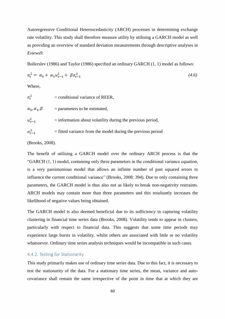
60

Autoregressive Conditional Heteroscedasticity (ARCH) processes in determining exchange

rate volatility. This study shall therefore measure utility by utilising a GARCH model as well

as providing an overview of standard deviation measurements through descriptive analyses in

Eviews9.

Bollerslev (1986) and Taylor (1986) specified an ordinary GARCH (1, 1) model as follows:

(4.6)

Where,

= conditional variance of REER,

= parameters to be estimated,

= information about volatility during the previous period,

= fitted variance from the model during the previous period

(Brooks, 2008).

The benefit of utilising a GARCH model over the ordinary ARCH process is that the

“GARCH (1, 1) model, containing only three parameters in the conditional variance equation,

is a very parsimonious model that allows an infinite number of past squared errors to

influence the current conditional variance” (Brooks, 2008: 394). Due to only containing three

parameters, the GARCH model is thus also not as likely to break non-negativity restraints.

ARCH models may contain more than three parameters and this resultantly increases the

likelihood of negative values being obtained.

The GARCH model is also deemed beneficial due to its sufficiency in capturing volatility

clustering in financial time series data (Brooks, 2008). Volatility tends to appear in clusters,

particularly with respect to financial data. This suggests that some time periods may

experience large bursts in volatility, whilst others are associated with little or no volatility

whatsoever. Ordinary time series analysis techniques would be incompatible in such cases.

4.4.2. Testing for Stationarity

This study primarily makes use of ordinary time series data. Due to this fact, it is necessary to

test the stationarity of the data. For a stationary time series, the mean, variance and auto-

covariance shall remain the same irrespective of the point in time that at which they are

61

calculated (Gujarati and Porter, 2010). Problems arise in the use of non-stationary data, in

that a model that may appear to be a good fit becomes unreliable when examined under other

time periods. The use of non-stationary data can result in what is known as a spurious

regression, in that the application of normal estimation techniques to non-stationary data

reflects a model with a large value for , whilst the model itself is in fact valueless (Brooks,

2008).

4.4.2.1. Graphical Analysis

The stationarity of a time series can be tested through using stationarity and unit root tests;

these tests may be either formal or informal. Informal tests check for stationarity by plotting

time series data and looking for evidence of trend in mean, variance, autocorrelation and

seasonality (Brooks, 2008). This method essentially involves a subjective visual analysis of

data in graphical form. However, the downfall associated with informal tests is that they do

not provide clues as to the nature of the time series. As a result, formal unit root tests will

also need to be conducted.

4.4.2.2. Dickey-Fuller Test

The Dickey-Fuller test (DF) shall be discussed in order to provide a background to the

logistics behind the Augmented Dickey-Fuller test (ADF). Following Gujarati (2004), the DF

can be estimated in three various forms:

Random walk (4.7)

Random walk with drift (4.8)

Random walk with drift around stochastic trend (4.9)

The null hypotheses for the above three models is that the series contains a unit root ( =0)

suggesting non-stationarity, with the alternative being no presence of unit roots ( <0),

suggesting a stationary time series (Gujarati, 2004). If a unit root is found to be present, the

time series is considered to be nonstationary and the use of such data could result in a

spurious regression. In this case it would not be possible to reject the null hypothesis.

62

4.4.2.3. Augmented-Dickey Fuller Test

The weakness associated with the DF test discussed above arises from the assumption of the

error term being uncorrelated; should the error term be correlated, then the model should be

adjusted with the inclusion of a lagged dependent variable (Ramanathan, 1998). This

represents the notion behind the development of ADF, in that this form of the test augments

the DF equations through adding lagged values of the dependent variable. Specifically, the

ADF test can be illustrated by the following equation:

(4.10)

Where,

= white noise error term,

= (

, etc.

(Gujarati, 2004).

As with the DF test, the null hypothesis of a unit root being present would need to be rejected

in order for the time series to be deemed stationary. If the ADF tests were to confirm the

existence of a unit root in the series, it would then be necessary to calculate as to how many

times the series may need to be differenced in order to make it stationary (Brooks, 2008).

Once the level of differencing has been determined, the regression may be run in differenced

form. If no unit roots were found to exist, differencing would not be deemed necessary as the

time series is stationary.

4.4.2.4. Phillips-Perron Test

Phillips-Perron tests (PP) are similar to the ADF, but adjust ADF methodology to allow for

the presence of auto-correlated residuals (Gujarati, 2004). The PP tests build on from the

hypotheses developed under the DF tests, in that should a unit root be present the time series

is considered to be non-stationary. The level of differencing may once again first need to be

determined before the regression is run. Both the ADF and PP tests shall be utilised within

this study.

63

4.4.3. Co-integration Analysis

Co-integration is utilised to depict whether independent and dependent variables have a

stationary linear combination that implies a long run relationship. Considering the purpose of

this study is to determine the long-run relationship between REER volatility and variables

such as money supply and trade openness, co-integration analysis presents a fundamental

component of estimation techniques.

4.4.3.1. Johansen Co-integration Approach

The Johansen Co-integration Approach is the most commonly utilised technique in co-

integration determination in financial time series literature. Before this approach can be

utilised there are a number of steps which need to be followed, the first of which is testing the

order of integration of the variables being examined. The most favoured situation would be

one where variables are integrated of the same order, although this may not necessarily occur.

For example, a model may exist wherein there are two I(1) and two I(2) variables: “There is a

possibility that the two I(2) variables co-integrate down to an I(1) relationship, and then this

relationship may further co-integrate with one of the two I(1) variables to form another co-

integrating vector” (Asteriou and Hall, 2007: 322). Having variables that are integrated of

different orders makes measurement more complicated. The ADF and PP tests as discussed in

section 4.4.2 can be utilised to determine the order of integration of the model.

After testing the order of integration, the next step would be to determine an appropriate lag

length. A Vector Autoregressive (VAR) model containing variables in level form with a large

number of lags may first be estimated, followed by re-estimations containing less lags

(Asteriou and Hall, 2007). In each re-estimated model the Akaike Information Criterion

(AIC) and the Schwarz Bayesian Information Criterion (BIC) should be examined, and the

model which minimizes these criterion should be chosen (Asteriou and Hall, 2007). This

model would represent one which has an optimal number of lags.

Under the Johansen method, a multivariate model may be expressed as an unrestricted VAR

model with k number of lags in the form of:

(4.11)

Where,

= (n x 1) vector of endogenous variables,

64

= (n x n) matrix of co-efficient,

= (n x 1) vector of white noise error terms

(Asteriou and Hall, 2007).

The third step in Johansen methodology involves choosing an appropriate model regarding

deterministic components in a multivariate system. The non-stationarity of economic time

series requires that equation 4.11 needs to be transformed into a Vector Error Correction

Model (VECM), such as:

(4.12)

Where contains information on the short run dynamics and contains information on the

long run dynamics. More specifically:

(4.13)

Where represents the speed of adjustment to disequilibrium and is a matrix of co-

integrating vectors that ensure the convergence of to their long run steady state solutions

(Asteriou and Hall, 2007). Given equation 4.12, three possible models exist. There may be “a

constant (with co-efficient ) and/or a trend (with co-efficient ) in the long run model (the

co-integrating equation (CE)), and a constant (with co-efficient ) and/or a trend (with co-

efficient ) in the short run model (VAR model)” (Asteriou and Hall, 2007: 323). In order to

determine which case is most suitable, all three models should be estimated and compared to

trace statistics.

In order to determine the presence of co-integration, the matrix coefficients are compared to

their eigenvalues. The fourth step in Johansen methodology involves determining the rank of

matrix coefficients. There are two possible methods, which can be specified as follows:

(4.14)

And

(4.15)

Where,

r = number of co-integrating vectors,

65

= estimated value for ith ordered eigenvalue

(Brooks, 2008).

The trace test thus tests the hypothesis that there are at maximum r co-integrating vectors,

whilst the maximum eigenvalue test tests the hypothesis that there are r+1 co-integrating

vectors against the hypothesis that there are r co-integrating vectors. Thus the Johansen

method has the added advantage of being able to identify more than one co-integrating

vector, which overcomes one of the main downfalls associated with the Engle Granger

approach to estimating co-integrating relationships (Brooks, 2008).

According to Brooks (2008: 352): “If the test statistic is greater than the critical value from

Johansen’s tables, reject the null hypothesis that there are r co-integrating vectors in favour of

the alternative that there are r+1 (for or more than r (for . In this manner it is

possible to identify all the co-integrating vectors present in the model. After these co-

integrating vectors have been estimated, a VECM model can then be estimated by specifying

the total number of co-integrating vectors.

Step five of the Johansen approach involves testing for weak exogeneity; if a variable is

determined to be weakly exogenous this variable may then be dropped as an endogenous part

of the multivariate system (Asteriou and Hall, 2007). The last step in Johansen methodology

is testing for linear restrictions in the co-integrating vectors. More specifically, estimates of

and are obtained through Johansen measurements and tested for any restrictions (Asteriou

and Hall, 2007).

4.4.3.2. Vector Error Correction Model

Once the presence of co-integration has been established and the number of co-integrating

vectors determined, it is then possible to specify the VECM for this study. The use of the

VECM approach is based on the study conducted by Ajao and Igbekoyi (2013). The main

reasoning behind the theory of VECM’s is that there is often a long run relationship between

variables, despite short run periods of disequilibrium (Ramanathan, 1998). What this short

run disequilibrium refers to is that these variables may deviate from their relationship in the

short run, but in the long run it still tends to hold. A VECM model can be used to correct

these short run deviations in the long term, and can generally be expressed as follows:

(4.16)

66

Where,

= error correction term,

= long run relationship between x and y,

= short run relationship between Δ x and Δ y,

= speed of adjustment back to equilibrium

(Brooks, 2008).

The VECM for this study can thus be specified as:

(4.17)

Where,

= white noise error term,

= error correction term,

= long run effects,

, , etc. = short run effects.

4.4.4. Diagnostic Tests

It is important to analyse the behaviour of each model so as to determine the extent to which

one can rely on the results that have been estimated. The diagnostic tests that have been

deemed relevant for this study are: serial correlation, heteroscedasticity, normality, impulse

response analysis and variance decomposition.

67

4.4.4.1. Serial Correlation

The LM-ARCH test may be described as a test which is utilised to detect the presence of

autocorrelation, with Ordinary Least Squares (OLS) methodology requiring that the error

terms in a time series need to be uncorrelated (Gujarati and Porter, 2010). Should

autocorrelation be present, it would thus have the resulting consequence of OLS and normal

regression techniques such as the t and F tests being unreliable.

4.4.4.2. Whites Heteroscedasticity Test

A further assumption of the classical regression model is that homoscedasticity is present,

which implies that the variance of the error terms is constant (Brooks, 2008). Should the

variance not be constant, heteroscedasticity is thus deemed to exist. In such a case ordinary

regression techniques would not be compatible. One could graphically plot the residuals to

determine whether a pattern exists, but formal testing would be more accurate rather than

relying on visual observations.

One of the methods that can be utilised to detect the presence of homoscedasticity is Whites

test. The null hypothesis of White’s test is that the error terms are homoscedastic, whilst the

alternative hypothesis is that the error terms are heteroscedastic (Brooks, 2008). Whites test is

a more commonly used measure of homoscedasticity and shall be utilised for the purposes of

this study.

4.4.4.3. Residual Normality Test

A normality test is applied to determine if the error terms are normally distributed. The

Jarque Bera (JB) tests “…whether the co-efficient of skewness and the co-efficient of excess

kurtosis are jointly zero” (Brooks, 2008: 163). If both skewness (S) and kurtosis (K-3) are

equal to zero, then the distribution of the time series data is considered to be normal. This test

can indicated by the following equation:

(4.18)

Where,

n = sample size,

S = skewness,

68

K = kurtosis

(Gujarati and Porter, 2010).

Should skewness or kurtosis be higher than zero, then the value of the JB statistic would start

to rise. The null hypothesis of normality should be rejected if the measure of the JB statistic is

higher than the critical value of two degrees of freedom (Gujarati and Porter, 2010). In such a

case, the distribution is not considered to be normal.

4.4.4.4. Impulse Response Analysis

Impulse response analysis involves observing the response of a dependent variable to shocks

in error terms (Asteriou and Hall, 2007). Impulse response functions thus illustrate the

magnitude and persistence of shocks over a specific period of time. The identification

problem from impulse response analysis arises because: “(i) one has to allow for

interdependent dynamics…and (ii) one has to identify the correct shock from unobservable

data” (Hill, Griffiths and Lim, 2012: 506). In this study impulse response analysis shall be

applied to the VECM model in the form of the Choleski approach.

4.4.4.5. Variance Decomposition

Whilst the impulse response analysis traces the sensitivity of the dependent variable to

shocks, variance decomposition analysis provides information on the relative significance of

each shock to the system (Enders, 1995). As with the impulse response analysis, the Choleski

approach is to be utilised.

4.5. Conclusion

This chapter specified the model that is to be utilised in determining factors that impact

REER volatility in South Africa. Included in this model are variables that are highly likely to

impact the level of volatility in the exchange rate. These variables include government

expenditure, money supply, trade openness, economic growth, an inflation rate differential

and a real interest rate differential.

the ADF and PP tests will be employed in testing stationarity. Volatility measures such as the

GARCH (1, 1) process and standard deviation techniques will be used. The estimation

technique to be utilised is the VECM as based on previous empirical studies, accompanied by

co-integration analysis by means of the Johansen Co-integration Approach. Lastly, the

69

chapter concluded with a discussion on diagnostic tests, such as the LM test, Whites

Heteroscedasticity test, the JB test and impulse response and variance decomposition

analyses. Chapter five will focus on an examination of the results after the regression has

been run through Eviews9.

70

Chapter Five

Empirical Analysis and Findings

5.1. Introduction

Chapter four presented the specified models and provided an analysis of various econometric

techniques that are to be utilised for the purposes of this study. This chapter presents the

results obtained from empirical analysis. These results are meant to ensure the attainment of

the study’s objectives by determining which variables are responsible for causing volatility in

the real effective exchange rate (REER). This chapter is divided into various subsections.

Section 5.2 presents an analysis of descriptive statistics. Section 5.3 indicates the results of

stationarity testing. The Generalized Autoregressive Conditional Heteroscedasticity

(GARCH) model provides a measurement for volatility, whilst the Johansen estimation

technique and the Vector Error Correction Model (VECM) explain the relationship between

the REER and related variables. In order to determine the policy implications arising from the

empirical results obtained, impulse response and variance decomposition analysis are

presented in sections 5.7 and 5.8. The chapter is concluded by means of a summarisation of

estimation techniques in section 5.9.

5.2. Descriptive Statistics

Table 5.1 shows the descriptive statistics of LREEXR. The Jarque-Bera (JB) normality test

assumes that perfectly symmetric residuals will have a skewness of 0, and that normally

distributed residuals will display kurtosis values of 3 (Hill, Griffiths and Lim, 2012). The

LREEXR value for skewness is -0.5382 which implies negative skewness. A negative skew

indicates that the tail on the left hand side is longer than the tail on the right hand side and the

bulk of the values lie to the right of the mean. The coefficient of LREEXR thus indicates that

there is slight asymmetry in LREEXR.

Kurtosis refers to the peakedness of distribution (Hill, Griffiths and Lim, 2012). The value of

kurtosis for LREEXR is 2.7916, which is only slightly different from 3. The question now

remains as to whether 2.7916 is sufficiently different from 3, and whether -0.5382 is

sufficiently different from 0 in order to conclude that the residuals are not normally

distributed. The p-value of the JB statistic is 0.1220 which is greater than 5%. Therefore it is

possible to accept the null hypothesis of normal distribution for LREEXR.

71

By examining the standard deviation value for LREEXR, it may be observed that the

exchange rate is slightly volatile. The standard deviation value is 0.1086, and although this

value is not significantly large it still illustrates the presence of slight volatility in the

exchange rate.

Table 5.1: Descriptive Statistics

Variable LREEXR

Mean 4.516

Standard

deviation

0.1086

Skewness -0.5382

Kurtosis 2.7916

J.B.

P value

4.207

0.1220

Source: Authors own computation

In order to measure volatility, Al Samara (2009) combined both standard deviation

techniques and a form of ARCH processes. The GARCH process was discussed in Section

4.4.1. Considering that the descriptive statistics in Table 5.1 indicate the need for a volatility

measure of the exchange rate, a new series LREEXRVOL was thus created using the

GARCH approach.

5.3. Stationarity Test

As discussed in the previous chapter, stationary testing is necessary to prevent spurious

regressions from occurring and to assist in determining the estimation techniques that are

applicable to the study. Both formal and informal stationarity tests were utilised. Informal

testing involves graphical analysis, whilst formal testing is conducted by means of the

Augmented Dickey-Fuller (ADF) and Phillips Perron (PP) tests.

5.3.1. Graphical Analysis

One method of determining whether or not a series is stationary is through plotting the series

against time. Should a graph cross the mean value multiple times, the variable is most likely

stationary. However, if that does not happen it would suggest that there are persistent trends

in the underlying data. In order to detect whether the exchange rate and related variables are

stationary, graphical plots of data in level form are presented in Figure5.1.

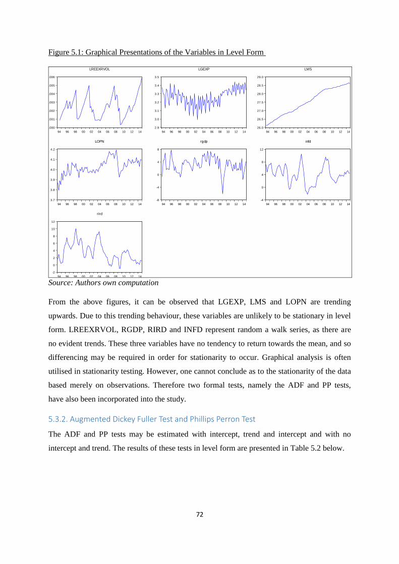
72

Figure 5.1: Graphical Presentations of the Variables in Level Form

.000

.001

.002

.003

.004

.005

.006

94 96 98 00 02 04 06 08 10 12 14

LREEXRVOL

2.9

3.0

3.1

3.2

3.3

3.4

3.5

94 96 98 00 02 04 06 08 10 12 14

LGEXP

26.0

26.5

27.0

27.5

28.0

28.5

29.0

94 96 98 00 02 04 06 08 10 12 14

LMS

3.7

3.8

3.9

4.0

4.1

4.2

94 96 98 00 02 04 06 08 10 12 14

LOPN

-8

-4

0

4

8

94 96 98 00 02 04 06 08 10 12 14

rgdp

-4

0

4

8

12

94 96 98 00 02 04 06 08 10 12 14

infd

-2

0

2

4

6

8

10

12

94 96 98 00 02 04 06 08 10 12 14

rird


From the above figures, it can be observed that LGEXP, LMS and LOPN are trending

upwards. Due to this trending behaviour, these variables are unlikely to be stationary in level

form. LREEXRVOL, RGDP, RIRD and INFD represent random a walk series, as there are

no evident trends. These three variables have no tendency to return towards the mean, and so

differencing may be required in order for stationarity to occur. Graphical analysis is often

utilised in stationarity testing. However, one cannot conclude as to the stationarity of the data

based merely on observations. Therefore two formal tests, namely the ADF and PP tests,

have also been incorporated into the study.

5.3.2. Augmented Dickey Fuller Test and Phillips Perron Test

The ADF and PP tests may be estimated with intercept, trend and intercept and with no

intercept and trend. The results of these tests in level form are presented in Table 5.2 below.

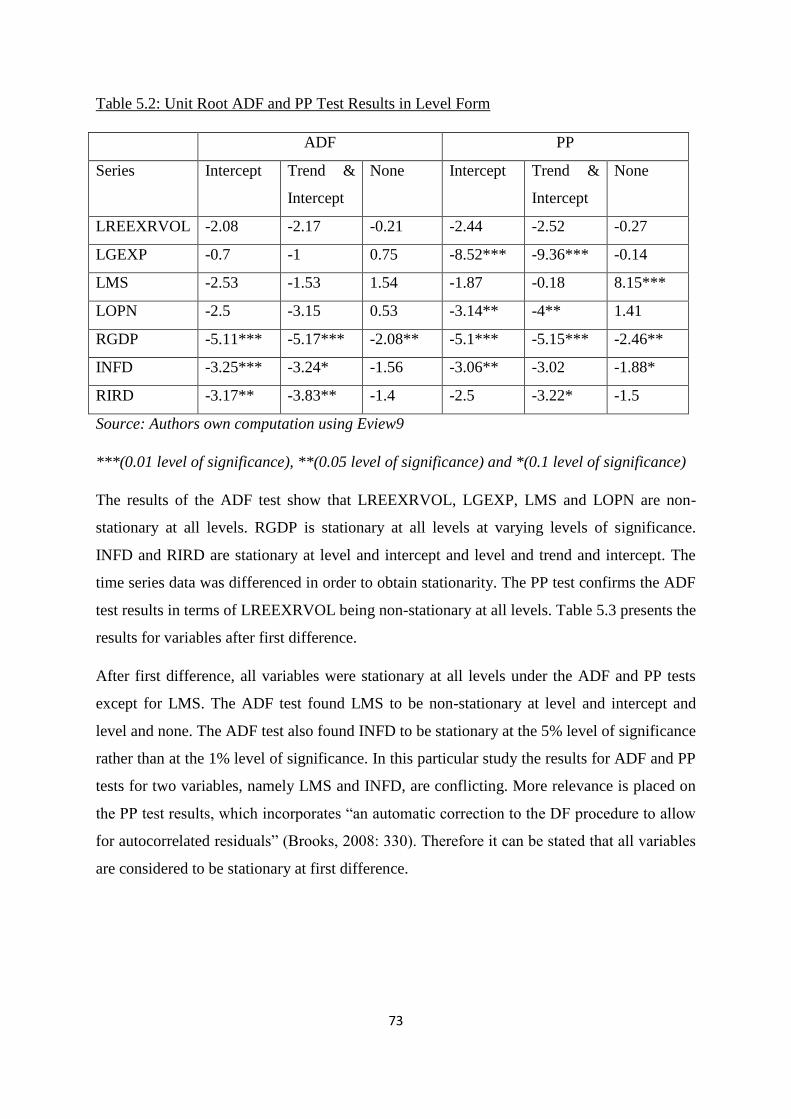
73

Table 5.2: Unit Root ADF and PP Test Results in Level Form

ADF PP

Series Intercept Trend &

Intercept

None Intercept Trend &

Intercept

None

LREEXRVOL -2.08 -2.17 -0.21 -2.44 -2.52 -0.27

LGEXP -0.7 -1 0.75 -8.52*** -9.36*** -0.14

LMS -2.53 -1.53 1.54 -1.87 -0.18 8.15***

LOPN -2.5 -3.15 0.53 -3.14** -4** 1.41

RGDP -5.11*** -5.17*** -2.08** -5.1*** -5.15*** -2.46**

INFD -3.25*** -3.24* -1.56 -3.06** -3.02 -1.88*

RIRD -3.17** -3.83** -1.4 -2.5 -3.22* -1.5

Source: Authors own computation using Eview9

***(0.01 level of significance), **(0.05 level of significance) and *(0.1 level of significance)

The results of the ADF test show that LREEXRVOL, LGEXP, LMS and LOPN are non-

stationary at all levels. RGDP is stationary at all levels at varying levels of significance.

INFD and RIRD are stationary at level and intercept and level and trend and intercept. The

time series data was differenced in order to obtain stationarity. The PP test confirms the ADF

test results in terms of LREEXRVOL being non-stationary at all levels. Table 5.3 presents the

results for variables after first difference.

After first difference, all variables were stationary at all levels under the ADF and PP tests

except for LMS. The ADF test found LMS to be non-stationary at level and intercept and

level and none. The ADF test also found INFD to be stationary at the 5% level of significance

rather than at the 1% level of significance. In this particular study the results for ADF and PP

tests for two variables, namely LMS and INFD, are conflicting. More relevance is placed on

the PP test results, which incorporates “an automatic correction to the DF procedure to allow

for autocorrelated residuals” (Brooks, 2008: 330). Therefore it can be stated that all variables

are considered to be stationary at first difference.

74

Table 5.3: Unit Root ADF and PP Test Results in First Difference Form

ADF PP

Series Intercept Trend &

Intercept

None Intercept Trend &

Intercept

None

LREEXRVOL -9.22*** -9.2*** -9.22*** -9.22*** -9.2*** -9.22***

LGEXP -4.07*** -20.88*** -4.06*** -49.7*** -67.5*** -49.48***

LMS -1.93 -7.17*** -1.04 -6.9*** -7.45*** -2.98***

LOPN -4.35*** -4.3*** -4.34*** -14.03*** -14.81*** -13.42***

RGDP -12.12*** -12.03*** -12.19*** -16.36*** -16.19*** -16.51***

INFD -3.78*** -3.76** -3.81*** -5.56*** -5.15*** -5.6***

RIRD -6.5*** -6.54*** -6.55*** -6.03*** -5.98*** -6.08***


***(0.01 level of significance), **(0.05 level of significance) and *(0.1 level of significance)

Figure 5.2 shows that all variables have a tendency to revert to mean values after first

differencing occurs. Despite fluctuations around the mean in the short term, variables are

considered to be stationary in the long run with a constant mean and constant variance.

Second differencing is therefore not required, and all variables are considered to be integrated

of the same order. All variables are integrated of order I (1). It is therefore possible to

continue with co-integration testing.

75

Figure 5.2: Graphical Presentation of the Variables in First Difference Form

-.004

-.003

-.002

-.001

.000

.001

94 96 98 00 02 04 06 08 10 12 14

Differenced LREEXRVOL

-.3

-.2

-.1

.0

.1

.2

.3

94 96 98 00 02 04 06 08 10 12 14

Differenced LGEXP

-.02

.00

.02

.04

.06

.08

.10

94 96 98 00 02 04 06 08 10 12 14

Differenced LMS

-.15

-.10

-.05

.00

.05

.10

.15

94 96 98 00 02 04 06 08 10 12 14

Differenced LOPN

-8

-6

-4

-2

0

2

4

6

94 96 98 00 02 04 06 08 10 12 14

Differenced rgdp

-6

-4

-2

0

2

4

94 96 98 00 02 04 06 08 10 12 14

Differenced infd

-3

-2

-1

0

1

2

3

4

94 96 98 00 02 04 06 08 10 12 14

Differenced rird


5.4. Co-integration Test

The co-integration analysis was conducted using the Johansen technique. This test was

utilised in order to determine whether a long run relationship exists between REER volatility

and related variables. However, before co-integrating relationships can be established, there

are a number of steps that need to be employed. These steps are: (1) Determining the order of

integration; (2) Choosing an appropriate lag length; (3) Choosing an appropriate model based

on deterministic components in a multivariate system; (4) Establishing the rank of matrix

coefficients; (5) Testing for weak exogeneity; and (6) Testing for linear restrictions in the co-

integrating vectors (Asteriou and Hall, 2007).

5.4.1. Order of Integration

The first step in the Johansen technique involves determining the order of integration of the

variables. Based on both formal (the ADF and PP tests) and informal (graphical analysis) unit

root tests, all variables may be stated as being integrated of order one. Variables were found

76

to all be stationary after first differencing. Having variables integrated of the same order

makes measurements less complicated.

5.4.2. Optimal Lag Length Selection Criteria

In this particular study Akaike Information Criterion (AIC), Schwarz Information Criterion

(SIC), Hannan Quinn Criterion (HIQ), Final Prediction Error (FPE) as well as Likelihood

Ratio Test (LR) were utilised in selecting an optimal lag length. Table 5.4 presents the results

obtained from the aforementioned criterion tests. The LR, FPE, AIC and HQ selected 7 lags,

whilst the SC selected 1 lag. Brooks (2002: 427) believes that this problem arises due to a

small sample bias. In this study it was decided to utilise both 1 and 7 lags in order to

determine which model fits theoretical priors more sufficiently.

Table 5.4: VAR Lag Selection

Lag LogL LR FPE AIC SC HQ 0 35.58254 NA 1.10e-09 -0.762201 -0.545902 -0.675835

1 542.5121 905.7142 5.51e-15 -12.97366 -11.24327* -12.28273

2 621.1645 125.8439 2.58e-15 -13.76439 -10.51990 -12.46890

3 661.3260 56.76152 3.56e-15 -13.52869 -8.770117 -11.62865

4 740.5500 97.18147 1.89e-15 -14.33467 -8.061999 -11.83006

5 812.5231 74.85198 1.39e-15 -14.94728 -7.160522 -11.83811

6 893.6895 69.26202 9.77e-16 -15.80505 -6.504201 -12.09132

7 1011.678 78.65884* 3.54e-16* -17.64474* -6.829795 -13.32645* * indicates lag order selected by the criterion

LR: sequential modified LR test statistic (each test at 5% level)

FPE: Final prediction error

AIC: Akaike information criterion

SC: Schwarz information criterion

HQ: Hannan-Quinn information criterion


5.4.3. Deterministic Trend Assumption

The Pantula Principle Test was applied in order to determine the deterministic trend that was

suitable for analysis. The Pantula Principle Test involves using the Trace test statistic in

testing the null hypothesis of zero co-integrating vectors for the most restrictive model.

Should the null be rejected, the same test is considered for less restrictive models. Should the

hypothesis be rejected for the least restrictive model, the procedure would continue through

testing the null hypothesis of at most one co-integrating vector from the most restricted model

to the least restricted model. This procedure will discontinue at the point where it is not

possible to reject the null hypothesis for the first time (Asteriou and Hall, 2007).

77

The three possible models under consideration are (1) restricted intercepts and no trend, (2)

unrestricted intercepts and no trend and (3) unrestricted intercepts and restricted trends

(Asteriou & Hall, 2007). The results for the Pantula Principle Test are displayed in Table 5.5

below.

Table 5.5: The Pantula Principle Test Results

R n-r Model 2 Model 3 Model 4

Trace

Statistic

Critical

Value

Trace

Statistic

Critical

Value

Trace

Statistic

Critical

Value

0 7 404.5961 134.6780 391.2329 125.6154 496.2795 150.5585

1 6 252.0142 103.8473 243.5047 95.75366 288.2327 117.7082

2 5 175.1637 76.97277 167.7633 69.81889 192.6685 88.80380

3 4 117.6033 54.07904 110.9245 47.85613 126.2076 63.87610

4 3 61.67606 35.19275 55.23757 29.79707 69.48688 42.91525

5 2 29.14299 20.26184 22.78140 15.49471 36.58064 25.87211

6 1 7.735554* 9.164546 2.326909 3.841466 12.33086 12.51798


Note: * indicates the first time that the null cannot be rejected

Based on the results presented in Table 5.5, the Johansen co-integration test was conducted

under the assumption of restricted intercepts and no trends. This represents Model 2, which

was chosen according to the Pantula Principle. There are at most 6 co-integrating vectors

with no deterministic trends in the data at level form. The null hypothesis was rejected at the

point where the trace statistic of 7.735554 was less than the 5% critical value of 9.164546.

5.4.4. Determination of the Rank of ∏

The next step involves determining the rank of the matrix coefficients. The top part of Table

5.6 indicates the Johansen test based on trace test statistics, whilst the bottom part illustrates

the results based on maximum eigenvalue statistics. By beginning with the trace test it is

possible to observe that the null hypothesis of no co-integrating vectors is rejected as the

trace test statistic of 404.5961 is greater than the 5% critical value of 134.6780. The null

hypothesis of there being at most 6 co-integrating vectors cannot be rejected, as the trace test

statistic of 7.735554 is less than the 5% critical value of 9.164546. Therefore the trace test

indicates that there are at most 6 co-integrating vectors (relationships) at the 5% level.

In terms of the maximum eigenvalue test, it is possible to observe that the null hypothesis of

no co-integrating vectors is rejected as the maximum eigenvalue test statistic of 152.5820 is

greater than the 5% critical value of 47.04897. The null hypothesis of there being at most 6

co-integrating vectors cannot be rejected, as the maximum eigenvalue statistic of 7.73554 is

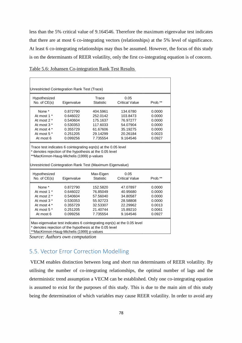
78

less than the 5% critical value of 9.164546. Therefore the maximum eigenvalue test indicates

that there are at most 6 co-integrating vectors (relationships) at the 5% level of significance.

At least 6 co-integrating relationships may thus be assumed. However, the focus of this study

is on the determinants of REER volatility, only the first co-integrating equation is of concern.

Table 5.6: Johansen Co-integration Rank Test Results

Unrestricted Cointegration Rank Test (Trace) Hypothesized Trace 0.05

No. of CE(s) Eigenvalue Statistic Critical Value Prob.** None * 0.872790 404.5961 134.6780 0.0000

At most 1 * 0.646022 252.0142 103.8473 0.0000

At most 2 * 0.540604 175.1637 76.97277 0.0000

At most 3 * 0.530353 117.6033 54.07904 0.0000

At most 4 * 0.355729 61.67606 35.19275 0.0000

At most 5 * 0.251205 29.14299 20.26184 0.0023

At most 6 0.099256 7.735554 9.164546 0.0927 Trace test indicates 6 cointegrating eqn(s) at the 0.05 level

* denotes rejection of the hypothesis at the 0.05 level

**MacKinnon-Haug-Michelis (1999) p-values

Unrestricted Cointegration Rank Test (Maximum Eigenvalue) Hypothesized Max-Eigen 0.05


At most 1 * 0.646022 76.85049 40.95680 0.0000

At most 2 * 0.540604 57.56040 34.80587 0.0000

At most 3 * 0.530353 55.92723 28.58808 0.0000

At most 4 * 0.355729 32.53307 22.29962 0.0013

At most 5 * 0.251205 21.40744 15.89210 0.0061

At most 6 0.099256 7.735554 9.164546 0.0927 Max-eigenvalue test indicates 6 cointegrating eqn(s) at the 0.05 level

* denotes rejection of the hypothesis at the 0.05 level **MacKinnon-Haug-Michelis (1999) p-values


5.5. Vector Error Correction Modelling

VECM enables distinction between long and short run determinants of REER volatility. By

utilising the number of co-integrating relationships, the optimal number of lags and the

deterministic trend assumption a VECM can be established. Only one co-integrating equation

is assumed to exist for the purposes of this study. This is due to the main aim of this study

being the determination of which variables may cause REER volatility. In order to avoid any

79

bias of regression results by measurement errors, the co-integrating regression was

considered without imposition of symmetry and proportionality restrictions.

Table 5.7 presents the VECM results for two distinguishing models. For each specification,

only co-integration equation one was considered and discussed. The two models presented

differ in that different lag lengths were applied. Model 1 presents the results when lag length

was set at 1, in accordance with the SIC test. The SIC test imposes harsher penalties for

regressions incorporating more regressors which could explain why the findings differ from

those of other tests. Model 2 presents the results when lag length was set at 7, in accordance

with the findings of the LR, FPE, AIC and HQ tests.

Table 5.7: Long-run Co-integration Equation Results

Variable Model 1 Model 2

LGEXP -0.014609

[1.96224]

0.034118

[-5.49610]

LMS 0.004347

[-3.65538]

0.002406

[-3.29185]

LOPN -0.026438

[2.39974]

-0.057854

[9.88633]

RGDP -0.01620

[5.22077]

0.000996

[-2.86903]

INFD 0.000767

[-2.82046]

-0.001151

[3.25173]

RIRD 0.000750

[-2.68907]

0.000121

[-0.57946]


LGEXP is observed as having a significant and negative relationship with LREEXRVOL for

Model 1. The t-statistic value of 1.96224 is near the critical t-statistic of 2, resulting in the

variable being significant. Based on the results for Model 1, a one percentage increase in

national government expenditure will cause REER volatility to decrease by 0.0146 percent.

This negative relationship between LGEXP and LREEXRVOL is in line with the a priori

expectations for this study, based on research conducted by Mankiw (1987). Despite the t-

80

statistic being significant in Model 2, the co-efficient illustrates a positive relationship

between the two variables which is not in accordance with a priori expectations.

In terms of LMS, both models indicate a significant and positive relationship with

LREEXRVOL. A one percentage increase in money supply (M3 definition) will result in

REER volatility increasing by either 0.0043 or 0.0024 percent. The positive relationship

between M3 and exchange rate volatility matches the a priori expectations as defined in terms

of the findings by Chipili (2012).

With respect to LOPN, both models once again present similar results. LOPN is observed as

having a significant and negative relationship with LREEXRVOL. A one percentage increase

in trade openness will lead to REER volatility decreasing by either 0.0264 or 0.0578 percent.

This negative relationship is in line with the theoretical predictions outlined in the previous

chapter. Ajao and Igbekoyi (2013) emphasised the existence of a significant negative

relationship between trade openness and exchange rate volatility.

The results for RGDP differ between the two models. Economic growth is found to be

significant and having a negative relationship with exchange rate volatility under Model 1.

This finding is in accordance with theoretical predictions based on the study conducted by

Canales-Kriljenko and Habermeier (2004). A one percentage increase in RGDP will cause

LREEXRVOL to decrease by 0.0162 percent. In terms of Model 2, a significant yet positive

relationship between the two variables is observed.

According to Model 1, INFD has a significant and positive relationship with LREEXRVOL.

A one percentage increase in the inflation differential will cause exchange rate volatility to

increase by 0.0007 percent. For Model 2, INFD is found to have a significant and negative

relationship with LREEXRVOL. A one percentage increase in the inflation differential will

cause exchange rate volatility to decrease by 0.0011 percent. The model best suited in this

case is Model 1 as empirical studies such as Albuquerque and Portugal (2005) predict a

positive relationship.

The RIRD is observed as having a significant and positive relationship with LREEXRVOL.

Both models collaborate in terms of this finding, which is also in accordance with a priori

expectations as based on the study by Hacker, Kim and Mansson (2010). A one percentage

increase in the real interest rate differential will result in exchange rate volatility increasing

by either 0.0007 or 0.0001 percent.

81

Based on the findings above, Model 1 may clearly be observed as being better suited to this

investigation. All variables are found to be significant and in line with a priori expectations.

Despite all variables being significant for Model 2, the results for LGEXP, RGDP and INFD

were not in accordance with a priori expectations. Therefore only Model 1 shall be examined

for the remainder of this chapter.

Table 5.8: Short-run Co-integration Equation Results


The speed of adjustment is shown by the co-efficient of the error correction term in Table 5.8.

A negative co-efficient indicates that a variable is expected to converge to equilibrium in the

long term. LGEXP, RGDP and RIRD all have negative co-efficients, indicating that these

three variables will all converge to equilibrium in the long run. LREEXRVOL, LMS, LOPN

and INFD may all be observed as having positive co-efficients. However, the co-efficients of

these variables becomes negative in the second co-integrating equation. This means that these

variables are likely to return to equilibrium within the second quarter. Positive co-efficients in

the first quarter may be due to incomplete specifications. In order to obtain more information

about the short run, impulse response and variance decomposition analyses is necessary.

However, before these analyses may be completed it is important to test the efficiency of the

VECM through the use of diagnostic checks.

5.6. Diagnostic Checks

The necessity of diagnostic testing involves checking residuals of the series for any problems.

Should problems be present, this may indicate that the model is inefficient, and that

parameter estimates may be biased. Diagnostic checks included for the purposes of this

investigation are tests for serial correlation, heteroscedasticity, normality and testing for

stability by means of plotting AR roots graphs.

Error Correction: D(LREEXRV

OL) D(LGEXP) D(LMS) D(LOPN) D(RGDP) D(INFD) D(RIRD)

CointEq1 0.080118 -3.020582 1.370455 1.581233 -178.9751 118.8150 -66.84411

(0.01806) (2.37855) (0.51133) (1.18022) (59.4705) (32.5600) (33.2710)

[ 4.43580] [-1.26993] [ 2.68016] [ 1.33978] [-3.00948] [ 3.64911] [-2.00908]

D(LREEXRVOL(-1)) -0.285578 10.12018 -0.326548 -1.395926 55.11825 -100.3041 305.5486

(0.11401) (15.0140) (3.22768) (7.44989) (375.395) (205.528) (210.016)

[-2.50484] [ 0.67405] [-0.10117] [-0.18738] [ 0.14683] [-0.48803] [ 1.45488]

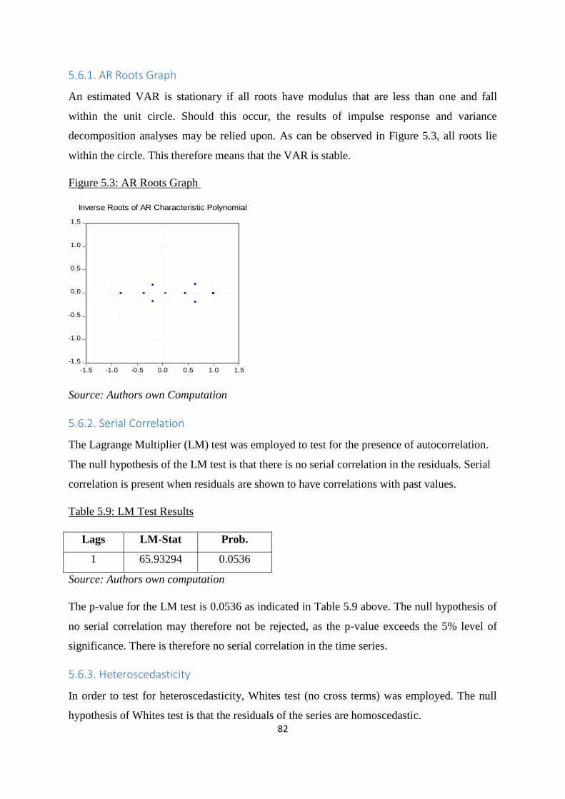
82

5.6.1. AR Roots Graph

An estimated VAR is stationary if all roots have modulus that are less than one and fall

within the unit circle. Should this occur, the results of impulse response and variance

decomposition analyses may be relied upon. As can be observed in Figure 5.3, all roots lie

within the circle. This therefore means that the VAR is stable.

Figure 5.3: AR Roots Graph

-1.5

-1.0

-0.5

0.0

0.5

1.0

1.5

-1.5 -1.0 -0.5 0.0 0.5 1.0 1.5

Inverse Roots of AR Characteristic Polynomial

Source: Authors own Computation

5.6.2. Serial Correlation

The Lagrange Multiplier (LM) test was employed to test for the presence of autocorrelation.

The null hypothesis of the LM test is that there is no serial correlation in the residuals. Serial

correlation is present when residuals are shown to have correlations with past values.

Table 5.9: LM Test Results

Lags LM-Stat Prob.

1 65.93294 0.0536


The p-value for the LM test is 0.0536 as indicated in Table 5.9 above. The null hypothesis of

no serial correlation may therefore not be rejected, as the p-value exceeds the 5% level of

significance. There is therefore no serial correlation in the time series.

5.6.3. Heteroscedasticity

In order to test for heteroscedasticity, Whites test (no cross terms) was employed. The null

hypothesis of Whites test is that the residuals of the series are homoscedastic.

83

Table 5.10: Heteroscedasticity Test Results

Joint Test:

Chi-sq. Df. Prob.

473.7271 448 0.1933


Table 5.10 illustrates the results obtained from conducting Whites test (no cross terms) for

heteroscedasticity. The p-value of 0.1933 indicates that the null hypothesis of homoscedastic

residuals cannot be rejected.

5.6.4. Normality

The Jarque-Bera (JB) tests were conducted to test for normality in the series. The null

hypothesis is that residuals are normally distributed. The results for the JB test are presented

in Table 5.11 below.

Table 5.11: JB Test Results

Chi-sq. Prob.

Skewness 26.99496 0.0000

Kurtosis 18.33756 0.0000

Jarque-Bera 45.33252 0.0000


As can be observed, the null hypothesis of normal distribution may be rejected due to the p-

value being less than 5%. This means that the residuals are not normally distributed.

Probabilities of Skewness (0.0000) and kurtosis (0.0000) corroborate this result of non-

normal distribution. However, this does not cause the results of the co-integration and VECM

tests to become invalid. The series is not normally distributed but still is efficient in terms of

no serial correlation and no heteroscedasticity being found present.

5.7. Impulse Response Analysis

The main objective of this study is to determine which variables are responsible for causing

exchange rate volatility. Therefore, only the response of exchange rate volatility to shocks in

its determinants are examined. The results of the impulse response analysis are presented in

Figure 5.4 below.

84

Figure 5.4: Impulse Response Results

-.0004

.0000

.0004

.0008

5 10 15 20 25 30 35

Response of LREEXRVOL to LREEXRVOL

-.0004

.0000

.0004

.0008

5 10 15 20 25 30 35

Response of LREEXRVOL to LGEXP

-.0004

.0000

.0004

.0008

5 10 15 20 25 30 35

Response of LREEXRVOL to LMS

-.0004

.0000

.0004

.0008

5 10 15 20 25 30 35

Response of LREEXRVOL to LOPN

-.0004

.0000

.0004

.0008

5 10 15 20 25 30 35

Response of LREEXRVOL to RGDP

-.0004

.0000

.0004

.0008

5 10 15 20 25 30 35

Response of LREEXRVOL to INFD

-.0004

.0000

.0004

.0008

5 10 15 20 25 30 35

Response of LREEXRVOL to RIRD

Response to Cholesky One S.D. Innovations


The results show that shocks to variables all die away in the long term at different rates. A

shock to LREEXRVOL causes a decrease in volatility and dies away around the 5th quarter.

A shock to LGEXP causes volatility to increase slightly but also dies away very quickly

around the 5th quarter. A shock to LMS causes volatility to immediately decrease but this dies

away before the 10th quarter is even reached. A shock to LOPN causes a moderate increase in

volatility. However, this shock dies away around the 5th quarter. A shock to RGDP causes a

rise in volatility but dies away before the 10th quarter. And a shock to either the INFD or

RIRD results in a decrease in volatility, but this dies away around the 5th quarter.

5.8. Variance Decomposition Analysis

Variance decomposition analysis may be utilised in order to determine the importance of

each shock in explaining variations in exchange rate volatility. Thirty six quarters were

examined in order to examine the relative effect of each variable on exchange rate volatility

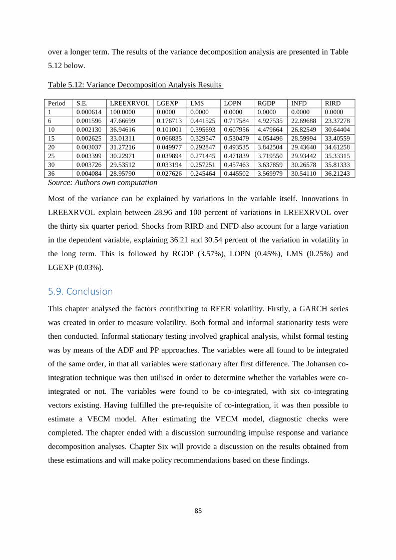
85

over a longer term. The results of the variance decomposition analysis are presented in Table

5.12 below.

Table 5.12: Variance Decomposition Analysis Results

Period S.E. LREEXRVOL LGEXP LMS LOPN RGDP INFD RIRD

1 0.000614 100.0000 0.0000 0.0000 0.0000 0.0000 0.0000 0.0000

6 0.001596 47.66699 0.176713 0.441525 0.717584 4.927535 22.69688 23.37278

10 0.002130 36.94616 0.101001 0.395693 0.607956 4.479664 26.82549 30.64404

15 0.002625 33.01311 0.066835 0.329547 0.530479 4.054496 28.59994 33.40559

20 0.003037 31.27216 0.049977 0.292847 0.493535 3.842504 29.43640 34.61258

25 0.003399 30.22971 0.039894 0.271445 0.471839 3.719550 29.93442 35.33315

30 0.003726 29.53512 0.033194 0.257251 0.457463 3.637859 30.26578 35.81333

36 0.004084 28.95790 0.027626 0.245464 0.445502 3.569979 30.54110 36.21243


Most of the variance can be explained by variations in the variable itself. Innovations in

LREEXRVOL explain between 28.96 and 100 percent of variations in LREEXRVOL over

the thirty six quarter period. Shocks from RIRD and INFD also account for a large variation

in the dependent variable, explaining 36.21 and 30.54 percent of the variation in volatility in

the long term. This is followed by RGDP (3.57%), LOPN (0.45%), LMS (0.25%) and

LGEXP (0.03%).

5.9. Conclusion

This chapter analysed the factors contributing to REER volatility. Firstly, a GARCH series

was created in order to measure volatility. Both formal and informal stationarity tests were

then conducted. Informal stationary testing involved graphical analysis, whilst formal testing

was by means of the ADF and PP approaches. The variables were all found to be integrated

of the same order, in that all variables were stationary after first difference. The Johansen co-

integration technique was then utilised in order to determine whether the variables were co-

integrated or not. The variables were found to be co-integrated, with six co-integrating

vectors existing. Having fulfilled the pre-requisite of co-integration, it was then possible to

estimate a VECM model. After estimating the VECM model, diagnostic checks were

completed. The chapter ended with a discussion surrounding impulse response and variance

decomposition analyses. Chapter Six will provide a discussion on the results obtained from

these estimations and will make policy recommendations based on these findings.

86

Chapter Six

Summary, Conclusions, Policy Implications and

Recommendations

87

6.1. Summary of the Study and Conclusions

The relevance of exchange rate volatility lies in the effect such variations have on other

important macroeconomic variables. For example, Ekanayake, Thaver and Plante (2012)

identified a harmful connection between trade flows and exchange rate volatility in South

Africa. This study examined the determinants of real effective exchange rate (REER)

volatility for South Africa. The study utilised quarterly data, beginning in 1994 and ending in

2014.

Variables for this study were chosen based on an assessment of relevant theoretical and

empirical literature. Theoretical literature included an examination of the purchasing power

parity theories, the monetary model, the portfolio balance approach and the balance of

payments theory. Empirical studies included (amongst others) those conducted by Canales-

Kriljenko and Habermeier (2004), De Jager (2012) and Ajao and Igbekoyi (2013).

The choice of the dependent variable, namely REER volatility is due to South Africa’s

numerous trading partner relations. An effective rate is able to capture volatility relating to a

number of currencies, rather than the study being based on a single bilateral exchange rate.

Explanatory variables chosen for the study were government expenditure (LGEXP), money

supply (LMS), trade openness (LOPN), economic growth (RGDP), an inflation rate

differential (INFD) and a real interest rate differential (RIRD).

After an assessment of existing literature it was then possible to specify the VAR model for

this study. In order to account for volatility in the model, it was first necessary to generate a

new volatility series (namely LREEXRVOL) using the Generalized Autoregressive

Conditional Heteroscedasticity (GARCH) approach. The time series data was then subject to

stationarity testing.

Stationarity tests conducted were both formal and informal. Informal tests were completed by

means of graphical analysis, whilst formal tests included the Augmented Dickey Fuller

(ADF) and Phillips Perron (PP) tests. The series was found to be stationary after first

difference, suggesting that all variables were also integrated of the same order. Co-integration

testing in the form of the Johansen technique was then applied, followed by regression

analysis by means of the Vector Error Correction Model (VECM) approach.

All explanatory variables were identified as being long run determinants of REER volatility

based on Model 1, which had a lag length of one. This model was chosen due to all variables

88

being significant and their respective co-efficients being of the correct sign in terms of

theoretical predictions. LGEXP, LOPN and RGDP were found to have negative relationships

with LREEXRVOL. The remaining explanatory variables LMS, INFD and RIRD all

displayed positive relationships with LREEXRVOL.

With respect to short run dynamics, LGEXP, RGDP and RIRD all return to their equilibrium

levels in the long term. On the other hand LREEXRVOL, LMS, LOPN and INFD all

displayed positive co-efficient values, meaning that disequilibrium in these variables

continues to grow. However, these variables were found to have negative co-efficient values

in the second quarter, suggesting that any disequilibrium was corrected for during this time.

Impulse response and variance decomposition analyses enabled a clearer picture of these

short run dynamics to be obtained.

According to the results of the impulse response analysis, shocks to all variables were found

to die away in the long term at different rates. Variance decomposition analysis revealed that

most of the variation in LREEXRVOL could be explained by innovations in the variable

itself. Over a thirty six quarter period, variations in LREEXRVOL caused between 28.96 and

100 percent of the variation in LREEXRVOL, followed by RIRD (36.21%), INFD (30.54%),

RGDP (3.57%), LOPN (0.45%), LMS (0.25%) and LGEXP (0.03%).

Diagnostic checks in the form of an AR roots graph revealed the VAR to be stable,

suggesting that the results of both impulse response and variance decomposition analyses

may be relied upon. The residuals were found to have no serial correlation and no

heteroscedasticity. However, the residuals were not found to be normally distributed. But this

does not render the results obtained from the co-integration and VECM approach invalid, as

the model is still considered efficient after having passed other diagnostic checks.

In summary, all explanatory variables chosen for this study were found to be significant in

having an effect on REER volatility. The relationship each variable had with LREEXRVOL

was also in alignment with theoretical predictions. As based on the empirical findings of the

study, it can be concluded that government expenditure, money supply, trade openness,

economic growth, inflation rate differentials and real interest rate differentials are all factors

significantly contributing to REER volatility.

89

6.2. Policy Implications and Recommendations

The results obtained from this study has numerous policy implications. It was found that

there exists a long term relationship between REER volatility and the chosen determinants.

This suggests that targeting any one of these explanatory variables may aid in reducing the

level of volatility experienced. One of the main objectives of the Accelerated and Shared

Economic Growth Initiative for South Africa (ASGISA) was to reduce rand volatility in order

to encourage economic growth (The Presidency of the Republic of South Africa, 2006).

Government may therefore need to practice sound macroeconomic policies in order to

achieve this objective.

The South African Reserve Bank (SARB) practice the policy of minimal intervention in the

foreign exchange market, with the rand primarily being determined by the level of demand

for and supply of foreign currency (SARB, 2014). Any deviation in the effective exchange

rate can thus be attributed to movements in one or more of the determinants. Government

spending, money supply, trade openness, economic growth, inflation rate differentials and

real interest rate differentials therefore need to be monitored in order to maintain a fair

exchange rate level.

Monetary policy in South Africa is practiced within an inflation targeting framework, with

inflation being allowed to fluctuate within a three to six percent bandwidth (Ricci, 2006). In a

bid to control inflation and maintain it within these levels, the Reserve Bank influences

variables such as money supply and/or the repurchase rate. The repo rate is considered an

operational variable, whereby an increase in the repo rate will lead to a decrease in price

levels (Van der Merwe and Mollentze, 2010). However, the downside is that this may result

in large unwarranted interest rate increases in a bid to control inflation.

According to Kahn (2008) and Du Plessis (2009) the inflation targeting regime in South

Africa has assisted in achieving both greater price stability and higher levels of economic

growth between 2000 and 2008, with the real interest rate appearing to be more stable during

this era than in previous time periods. Shocks to the inflation rate and real interest rate

differentials were found to contribute to 30.54% and 36.21% of the variation in REER

volatility. Therefore it is highly important to continue monitoring these variables in a bid to

control volatility levels. Monetary policy officials however do need to be cautious in altering

the repo rate in an effort to control inflation.

90

With respect to economic growth, a one percentage increase in growth will lead to REER

volatility decreasing by 0.0162 percent. As already stated, controlling inflation is proven to

have resulted in greater growth. Many policies aimed at higher growth rates have been

introduced into South Africa, namely: Growth, Employment and Redistribution (GEAR) in

1996; ASGISA in 2006; New Growth Path (NGP) in 2010; and more recently, the National

Development Plan (NDP) (Fourie and Burger, 2015). There is however concern regarding the

effectiveness of these growth policies. Greater attention needs to be had on implementation

and budgetary constraints in order for policies such as the NDP to be effective (Fourie and

Burger, 2015).

Trade liberalisation has been successful in terms of a reduction in tariffs and South Africa has

become a member country of a large number of trade agreements. However, Edwards and

Lawrence (2012) suggest that greater advantage needs to be taken of growth in emerging

markets and the African continent by making South African exports more accessible. By

increasing trade openness by one percent, REER volatility may be reduced by approximately

0.0264 percent.

Lastly, with respect to government spending, greater fiscal restraint needs to be exercised in

terms of re-prioritising key areas of expenditure. Government spending was found to have a

negative relationship with REER volatility, suggesting that a rise in spending will aid in

reducing volatility. However, spending needs to be allocated to areas that will result in

greater sustainability. The South African government have outlined the importance of re-

prioritising expenditure to core areas of service delivery (National Treasury, 2015).

6.3. Delimitations of the Study and Areas for Further Research

This particular study is focused on the South African economy, meaning that the model may

not necessarily be applicable to all other economies. However, despite this the study is still

relevant as it uncovers important variables that have an influence on exchange rate volatility

in the South African context. Some nations may have different economic structures and

exchange rate regimes to South Africa. Results may therefore be more relevant to countries

with flexible exchange rates (as is the South African case) rather than fixed rates.

This investigation also focuses on identifying quantitative factors or determinants that can

affect exchange rate volatility in South Africa. In stating that, non-quantifiable factors such as

political and social changes are not included within the model. For example, developments

91

such as union strikes that affect investor confidence and the exchange rate are not included

within the specified model equation.

Any lack of reliable information and data availability could affect measurement results. The

data obtained from various sources may need to be manipulated and not used in the original

format in which it was found. This could be because there is a lack of data in the form

required for the investigation, and therefore data that is available will need to be altered. For

example, this study specifically excluded the portfolio balance model as the data needed for

regression analysis was unlikely to be available.

Areas to consider for further research are:

1. Identifying the determinants of nominal effective exchange rate (NEER) volatility.

2. Determination of more efficient or suitable measures of volatility.

3. Identification of structural factors impacting volatility in South Africa.

92

REFERENCES

Ajao, M.G. & Igbekoyi, O.E. 2013. The Determinants of Real Exchange Rate Volatility in

Nigeria. Academic Journal of Interdisciplinary Studies, 2(1), 459-471.

Albuquerque, C.R. And Portugal, M. 2005. Exchange Rate and Inflation: A Case of Sulkiness

of Volatility. Available from: www.ufrgs.br/ppge/pcientifica/2005_01.pdf [Accessed: 16

May 2014]

Al Samara, M. 2009. The Determinants of Real Exchange Rate Volatility in the Syrian

Economy. Paris: Centre d’Economie de la sarbonne, universite Paris.

Appleyard, D.R., Field, A.J. & Cobb, S.L. 2010. International Economics. New York, United

States of America: McGraw-Hill/Irwin.

Asteriou, D. & Hall, S.G. 2007. Applied Econometrics A Modern Approach: Revised Edition.

New York: Palgrave Macmillan.

Asteriou, D. & Hall, S.G. 2011. Applied Econometrics A Modern Approach: Second Edition.

New York: Palgrave Macmillan.

Aziakpono, M.J. & Wilson, M.K. 2010. Interest Rate Pass-Through and Monetary Policy

Regimes in South Africa. Paper presented at CSAE Conference, 21-23 March 2010, Oxford

University UK: 1-43.

Bhorat, H., Hirsch, A., Kanbur, R. & Ncube, M. 2013. Economic Policy in South Africa Past,

Present and Future. In: Bhorat, H., Hirsch, A., Kanbur, R. & Ncube, M. eds. Oxford

Companion to the Economics of South Africa. South Africa: Oxford University Press, 1-27.

Bhundia, A. & Gottschalk, J. 2003. Sources of Nominal Exchange Rate Fluctuations in South

Africa. IMF Working Paper WP/03/252, 1-23.

Bhundia, A.J. & Ricci, L.A. 2006. The Rand Crises of 1998 and 2001: What Have We

Learned? In: Nowak, M. & Ricci, L.A. eds. Post-Apartheid South Africa: The First Ten

Years. Washington, DC: IMF, 156-173.

http://www.ufrgs.br/ppge/pcientifica/2005_01.pdf

93

Bleaney, M. 2006. Fundamentals and Exchange Rate Volatility. University of Nottingham

Discussion Papers in Economics No. 06/03, 1-16.

Brooks, C. 2008. Introductory Econometrics for Finance: Second Edition. New York, United

States of America: Cambridge University Press.

Burger, P. & Marinkov, M. 2008. Inflation targeting and inflation performance in South

Africa. Paper presented at 11th Annual Global Conference of The Competitive Institute, 29-31

October 2008, South Africa, 1-19.

Canales-Kriljenko, J. & Habermeier, K. 2004. Structural Factors Affecting Exchange Rate

Volatility: A Cross-section Study. IMF Working Paper WP/04/147, 1-13.

Chipili, J.M. 2012. Modelling Exchange Rate Volatility in Zambia. The African Finance

Journal, Africagrowth Institute, 14(2), 85-107.

Cushman, D.O. 2007. A Portfolio Balance Approach to the Canadian-US exchange rate.

Review of Financial Economics, 16(3), 305-320.

Daniels, J.P. & VanHoose, D.D. 2002. International Monetary & Financial Economics:

Second Edition. United States of America: South-Western Publishing.

Department of Finance. 1996. Growth, Employment and Redistribution. Pretoria: Department

of Finance, Republic of South Africa.

Ding, J. 2003. Exchange Rate Fluctuations and Economic Growth in Asia. World Economy,

(7), 15-22.

Dornbusch, R. 1985. Purchasing Power Parity. NBER Working Paper No. 1591, 1-34.

Du Plessis, S.P.J. 1998. International Economics: Second Edition. South Africa: Heinemann

Publishers (Pty) Ltd.

Edwards, L. & Lawrence, R. 2012. South African Trade Policy and the Future Global Trading

Environment. SAIIA Occasional Paper No. 128, 1-40.

Ekanayake, E.M, Thaver, R.L. & Plante, D. 2012. The Effects of Exchange Rate Volatility on

South Africa's Trade with the European Union. The International Journal of Business and

Finance Research, 6(3), 13-26.

Enders, W. 1995. Applied Econometric Time Series. Canada: John Wiley & Sons, Inc.

94

Fourie, F.C.N. & Burger, P. 2015. How to think and reason in Macroeconomics: Fourth

Edition. Cape Town, South Africa: Juta and Company (Pty) Ltd.

Frenkel, J.A. 1981. Flexible Exchange Rates, Prices and the Role of News: Lessons from the

1970s. Journal of Political Economy, 89(4), 665-705.

Gordhan, P. 2011. A Safer South African Sector to serve South Africa better. Available from:

http://www.treasury.gov.za/documents/national%20budget/2011/A%20safer%20financial%2

0sector%20to%20serve%20South%20Africa%20better.pdf [Accessed: 20 April 2015].

Gujarati, D.N. 2004. Basic Econometrics: Fourth Edition. New York, United States of

America: McGraw-Hill Companies.

Gujarati, D.N & Porter, D.C. 2010. Essentials of Econometrics: Fourth Edition. New York,

United States of America: McGraw-Hill/Irwin.

Hacker, R.S., Kim, H. & Mansson, K. 2010. An Investigation of the Causal Relations

between Exchange Rates and Interest Rate Differentials using Wavelets. CESIS Electronic

Working Paper Series Paper No. 215, 1-20.

Hanival, S. & Maia, J. 2008. An Overview of the Performance of the South African Economy

since 1994. Available from: http://www.thepresidency.gov.za/docs/reports/15year_review/

[Accessed: 5 June 2015].

Hill, R.C., Griffiths, W.E. & Lim, G.C. 2012. Principles of Econometrics: Fourth Edition.

United States of America: John Wiley & Sons, Inc.

Hilton, S. 2005. Trends in Federal Funds Rate Volatility. Federal Reserve Bank of New

York, Current Issues in Economics and Finance, 11(7), 1-7.

Hviding, K. 2006. Liberalizing Trade and Capital Transactions: An Overview. In: Nowak, M.

& Ricci, L.A. eds. Post-Apartheid South Africa: The First Ten Years. Washington, DC: IMF,

133-141.

IMF Staff. 1998. The Asian Crisis. World Economic Outlook, 18-21.

Industrial Development Corporation. Department of Research and Information. 2013. South

African economy: An overview of key trends since 1994. South Africa: IDC, 1-30.

http://www.thepresidency.gov.za/docs/reports/15year_review/

95

Industrial Development Corporation. Department of Research and Information. 2014.

Economic Overview: Recent Developments in the global and South African economies. South

Africa: IDC, 1-12.

Insah, B. & Chiaraah, A. 2013. Sources of real exchange rate volatility in the Ghanaian

economy. Journal of Economics and International Finance, 5(6), 232-238.

International Monetary Fund (IMF), International Financial Statistics (IFS). 2015. United

States Consumer Prices CPI% Change (IFS-I11164-XZFQ). Washington: IMF.

International Monetary Fund (IMF), International Financial Statistics (IFS). 2015. South

Africa Consumer Prices CPI% Change (IFS-I19964-XZFQ). Washington: IMF.

De Jager, S. 2010. Modelling South Africa’s equilibrium real effective exchange rate: A

VECM approach. SARB Working Paper WP/12/02, 1-23.

Kahn, B. & Farrell, G.N. 2002. South African Real Interest rates in comparative perspective:

theory and evidence. SARB Occasional Paper No. 17, 1-31.

Kahn, B. 2008. Challenges of inflation targeting for emerging market economies: The South

African case. Paper presented at SARB Conference, 29-31 October 2008, Pretoria.

Kahn, F.N. and Ahmad, E. 2005. Test of Purchasing Power Parity based on Co-integration

Technique: The Asian Evidence. Pakistan Economic and Social Review, 43(2), 167-183

Karoro, T.D., Aziakpono, M.J. & Cattaneo, N. 2009. Exchange rate pass-through to import

prices in South Africa: Is there asymmetry? South African Journal of Economics, 77(79),

380-398.

Kganyago, L. 2012. The Impact of the Eurozone and global financial crisis on South Africa.

Paper presented at Lereko Metier Capital Growth Fund Investor Conference, 1 March 2012,

Magaliesburg, South Africa, 1-6.

Kganyago, L. 2015. SA Monetary Policy Still Expansionary. Paper presented at Fedusa

Collective Bargaining Conference, 17 February 2015, Johannesburg, South Africa.

Koba, M. 2012. Federal Funds Rate. Available from: http://www.cnbc.com/id/46071997

[Accessed: 30 June 2015]

http://www.cnbc.com/id/46071997

96

Kumo, W., Rielander, J. & Omilola, B. 2014. African Economic Outlook. Available from:

http://www.africaneconomicoutlook.org/en/ [Accessed: 30 June 2015].

Lafrance, R., Osakwe, P. and St-Amant, P. 1998. Evaluating Alternative Measures of the Real

Effective Exchange Rate. Bank of Canada Working Paper No. 98-20, 1-21.

Lomahoza, K., Brockerhoff, S. & Frye, I. 2013. A Review of National and Provincial

Government Budgets in South Africa: Monitoring the Progressive Realisation of Socio-

Economic Rights Project. Studies in Poverty and Inequality Institute Working Paper 7, 1-44.

Mabugu, R. & Chitiga, M. 2007. South Africa trade liberalization and poverty in a dynamic

microsimulation CGE model. Department of Economics Working Paper Series 2007-18, 1-

43.

Mankiw, N. 2001. US monetary policy during the 1990s. National Bureau of Economic

Research Working Paper Series 8471, 1-59.

Marcus, G. 2014. Governor Gill Marcus: European Economics and Financial Centre

Distinguished Speakers Seminar. Available from:

http://www.gov.za/speeches/view.php?sid=44965 [Accessed: 1 July 2014].

Maswanganyi, N. 2014. Real interest rates “still supportive to economy.” Business Day, 13

August.

Matemba, L. 2002. Fall of the Rand. Paper presented at Southern African Catholic Bishops

Conference, February 2002, Cape Town, South Africa, 1-5.

McGregor, S. 2012. A zero interest rate world. Cape Town, South Africa: AllanGray,

Quarterly Commentary 1.

Mishkin, P. 2009. The Economics of Money, Banking and Financial Markets: Ninth Edition.

United States of America: Pearson.

Mohr, P. and Fourie, L. 2008. Economics for South African Students: Fourth Edition.

Pretoria: Van Schaik Publishers

Mohr, P. 2012. Understanding the Economy. Pretoria, South Africa: Van Schaik Publishers.

Money CNN. 2001. Fed Slashes Rates Again. Available from:

http://money.cnn.com/2001/10/02/economy/fed/ [Accessed: 8 June 2015].

http://www.africaneconomicoutlook.org/en/

http://www.gov.za/speeches/view.php?sid=44965

http://money.cnn.com/2001/10/02/economy/fed/

97

Mpofu, T.R. 2013. Real Exchange Rate Volatility and Employment Growth in South Africa:

The Case of Manufacturing. Paper presented at ECCE-USB Conference, Cape Town, South

Africa, 1-34.

National Treasury. 2015. National Budget. Available from:

http://www.treasury.gov.za/documents/national%20budget/2015/ [Accessed: 10 January

2016].

Neely, C. 2010. U.S. Historical Experience with Deflation. St Louis, America: Federal

Reserve Bank of St Louis, Economic Synopses No. 30.

Nowak, M. 2006. The First Ten Years After Apartheid: An Overview of the South African

Economy. In: Nowak, M. & Ricci, L.A. eds. Post-Apartheid South Africa: The First Ten

Years. Washington, DC: IMF, 1-10.

OECD. 2011. OECD Science, Technology and Industry Scoreboard. Available from:

doi:http://dx.doi.org/10.1787/sti_scoreboard-2011-en [Accessed: 20 October 2015].

Ogunleye, K. E. 2009. Exchange Rate Volatility and Foreign Direct Investment in Sub

Saharan Africa: Evidence from Nigeria and South Africa. Paper presented at CSAE

Conference Economic Development in Africa, 22-24 March 2009, Oxford, 1-22.

Organization for Economic Co-operation and Development (OECD), Monthly Economic

Indicators (MEI). 2015. Monetary aggregate M3 SA (MEI-ZAF_MARMM301_GPSAQ).

Paris: OECD Publishing.

Organization for Economic Co-operation and Development (OECD), Monthly Economic

Indicators (MEI). 2015. United States – Federal Funds Rate (MEI-USA_IRSTFR01_STQ).

Paris: OECD Publishing.

Papell, D.H. 2006. The Panel Purchasing Power Parity Puzzle. Journal of Money, Credit and

Banking, 38(2), 447-467.

Pilbeam, K. 1998. International Finance: Second Edition. London: MacMillan Press Ltd.

Poole, W. and Wheelock, D.C. 2008. Stable Prices, Stable Economy: Keeping Inflation in

Check Must Be No. 1 Goal of Monetary Policymakers. St Louis, America: Federal Reserve

Bank of St Louis, the Regional Economist.

http://www.treasury.gov.za/documents/national%20budget/2015/

98

Presidency of the Republic of South Africa. 2006. Accelerated and Shared Growth Initiative

for South Africa 2006 Annual Report. Available from:

http://www.thepresidency.gov.za/docs/asgisa2006.pdf [Accessed: 30 July 2015].

Ramanathan, R. 1998. Introductory Econometrics with Applications: Fourth Edition.

Orlando, Florida, United States of America: Harcourt Brace College Publishers.

Ramutloa, L. 2013. South Africa’s unemployment rate remains stubborn amidst a new

economic trajectory – Labour’s ALMB. South Africa: Department of Labour.

Ricci, L.A. 2006. Bringing Inflation under Control. In: Nowak, M. & Ricci, L.A. eds. Post-

Apartheid South Africa: The First Ten Years. Washington DC, IMF: 189-210.

Salvatore, D. 2007. International Economics: Ninth Edition. United States of America: John

Wiley & Sons, Inc.

Samson, M., Ampofo, S., Mac Quene, K., Ndlebe, A. & van Niekerk, I. 2003. The

fundamental determinants of the rand exchange rate: a historical and forward looking

analysis. Research paper commissioned by Strategy and Research Unit Trade and Investment

South Africa (TISA) Research Paper no. 36, 1-35.

SARB. 2002. Quarterly Bulletin, December 2002 no. 226. Pretoria, South Africa: SARB.

SARB. 2009. Quarterly Bulletin, June 2009 no. 252. Pretoria, South Africa: SARB.

SARB. 2013. Government Finance Statistics of South Africa: 1994-2012. Supplement to the

South African Reserve Bank Quarterly Bulletin. Pretoria, South Africa: SARB.

SARB. 2014. Quarterly Bulletin, December 2014 no. 274. Pretoria, South Africa: SARB.

SARB. 2015. Historical Macroeconomic Time Series Information (Code KBP5392M).

Pretoria, South Africa: SARB.

SARB. 2015. Historical Macroeconomic Time Series Information (Code: KBP4601E).


SARB. 2015. Historical Macroeconomic Time Series Information (Code: KBP5392Q).


http://www.thepresidency.gov.za/docs/asgisa2006.pdf

99

SARB. 2015. Historical Macroeconomic Time Series Information (Code: KBP6006S).


SARB. 2015. Historical Macroeconomic Time Series Information (Code: KBP6006C).






Sekantsi, L. 2011. The Impact of Real Exchange Rate Volatility on South African Exports to

the United States (U.S.): A Bounds Test Approach. Review of Economic and Business

Studies, 4(2), 119-139.

Sivy, M. 2012. Why Isn’t There More Inflation? TIME Magazine, 5 September.

Södersten, B. and Reed, G. 1994. International Economics: Third Edition. London:

Macmillan Press Ltd.

Solnik, B. and McLeavey, D. 2004. International Investments: Fifth Edition. United States of

America: Pearson Addison Wesley.

Stancik, J. 2006. Determinants of Exchange Rate Volatility: The Case of the New EU

Members. Czech Journal of Economics and Finance, 57(9-10), 414-432.

STANLIB. 2014. Global economic activity expected to improve. Available from:

http://www.stanlib.com/ECONOMICFOCUS/Pages/Globalecoactivityexpectedtoimprovein2

014.aspx [Accessed: 5 June 2015].

Statistics South Africa. 2014. National government spending breaks the R1 trillion mark.

Available from: http://www.statssa.gov.za/?p=2812 [Accessed: 22 June 2015].

Stephey, M.J. 2008. A Brief History of Bretton Woods System. TIME Magazine, 21 October.

Takaendesa, P.J. 2006. The Behaviour and Fundamental Determinants of the Real Exchange

Rate in South Africa. Unpublished Master’s Thesis. Grahamstown: Rhodes University.

http://www.stanlib.com/ECONOMICFOCUS/Pages/Globalecoactivityexpectedtoimprovein2014.aspx

http://www.stanlib.com/ECONOMICFOCUS/Pages/Globalecoactivityexpectedtoimprovein2014.aspx

http://www.statssa.gov.za/?p=2812

100

Terra, M.C.T. and de Abreu, A.L.V. 2005. Purchasing Power Parity: The Choice of Price

Index. Available:

http://bibliotecadigital.fgv.br/dspace/bitstream/handle/10438/785/2113.pdf?sequence=1

[Accessed: 25 January 2015].

Thurlow, J. 2006. Trade Liberalization and Pro-Poor Growth in South Africa. Trade and

Poverty Project, Southern Africa Labour and Development Research Unit, 1-24.

Van der Merwe, E.J. 1996. Exchange rate management policies in

South Africa: Recent experience and prospects. South African Reserve Bank Occasional

Paper No. 9. Pretoria: South African Reserve Bank.

Van der Merwe, E. & Mollentze, S. 2010. Monetary Economics in South Africa. Cape Town,

South Africa: Oxford University Press.

Weerasekera, Y.M.W.B. 1992. Nominal and real effective exchange rates for the SEACEN

countries. Kuala Lumpur: The South East Asian Central Banks (SEACEN) Research and

Training Centre.

QUANTEC Economic Forecast and Review (Quarterly Report and Data). 2015. Repo Rate

(SA) (QEF-RBR). Available from: http://www.easydata.co.za/data/timeseries/QEF-RBR/

[Accessed: 20 August 2015].

http://www.easydata.co.za/data/timeseries/QEF-RBR/

101

APPENDICES

Table 8.1: Johansen Co-integration Test Results for Model 2

Date: 12/13/15 Time: 15:49

Sample (adjusted): 1996Q3 2014Q4

Included observations: 74 after adjustments

Trend assumption: No deterministic trend (restricted constant)

Series: LREEXRVOL LGEXP LMS LOPN RGDP INFD RIRD

Lags interval (in first differences): 1 to 7



At most 1 * 0.646022 252.0142 103.8473 0.0000

At most 2 * 0.540604 175.1637 76.97277 0.0000

At most 3 * 0.530353 117.6033 54.07904 0.0000

At most 4 * 0.355729 61.67606 35.19275 0.0000

At most 5 * 0.251205 29.14299 20.26184 0.0023






At most 1 * 0.646022 76.85049 40.95680 0.0000

At most 2 * 0.540604 57.56040 34.80587 0.0000

At most 3 * 0.530353 55.92723 28.58808 0.0000

At most 4 * 0.355729 32.53307 22.29962 0.0013

At most 5 * 0.251205 21.40744 15.89210 0.0061





Date: 12/13/15 Time: 16:01



Trend assumption: Linear deterministic trend




No. of CE(s) Eigenvalue Statistic Critical Value Prob.**

102

None * 0.864167 391.2329 125.6154 0.0000

At most 1 * 0.640676 243.5047 95.75366 0.0000

At most 2 * 0.536103 167.7633 69.81889 0.0000

At most 3 * 0.528825 110.9245 47.85613 0.0000

At most 4 * 0.355059 55.23757 29.79707 0.0000

At most 5 * 0.241500 22.78140 15.49471 0.0034






At most 1 * 0.640676 75.74134 40.07757 0.0000

At most 2 * 0.536103 56.83884 33.87687 0.0000

At most 3 * 0.528825 55.68693 27.58434 0.0000

At most 4 * 0.355059 32.45617 21.13162 0.0009

At most 5 * 0.241500 20.45449 14.26460 0.0046





Date: 12/13/15 Time: 16:05



Trend assumption: Linear deterministic trend (restricted)





At most 1 * 0.725117 288.2327 117.7082 0.0000

At most 2 * 0.592665 192.6685 88.80380 0.0000

At most 3 * 0.535362 126.2076 63.87610 0.0000

At most 4 * 0.358970 69.48688 42.91525 0.0000

At most 5 * 0.279421 36.58064 25.87211 0.0016




Unrestricted Cointegration Rank Test (Maximum Eigenvalue)

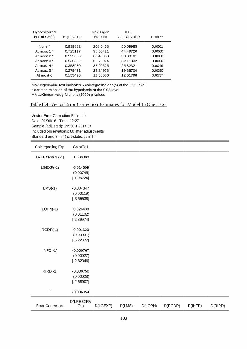
103

Hypothesized Max-Eigen 0.05


At most 1 * 0.725117 95.56421 44.49720 0.0000

At most 2 * 0.592665 66.46083 38.33101 0.0000

At most 3 * 0.535362 56.72074 32.11832 0.0000

At most 4 * 0.358970 32.90625 25.82321 0.0049

At most 5 * 0.279421 24.24978 19.38704 0.0090




Table 8.4: Vector Error Correction Estimates for Model 1 (One Lag)

Vector Error Correction Estimates

Date: 01/06/16 Time: 12:27



Standard errors in ( ) & t-statistics in [ ]

Cointegrating Eq: CointEq1

LREEXRVOL(-1) 1.000000

LGEXP(-1) 0.014609

(0.00745)

[ 1.96224]

LMS(-1) -0.004347

(0.00119)

[-3.65538]

LOPN(-1) 0.026438

(0.01102)

[ 2.39974]

RGDP(-1) 0.001620

(0.00031)

[ 5.22077]

INFD(-1) -0.000767

(0.00027)

[-2.82046]

RIRD(-1) -0.000750

(0.00028)

[-2.68907]

C -0.036054


OL) D(LGEXP) D(LMS) D(LOPN) D(RGDP) D(INFD) D(RIRD)

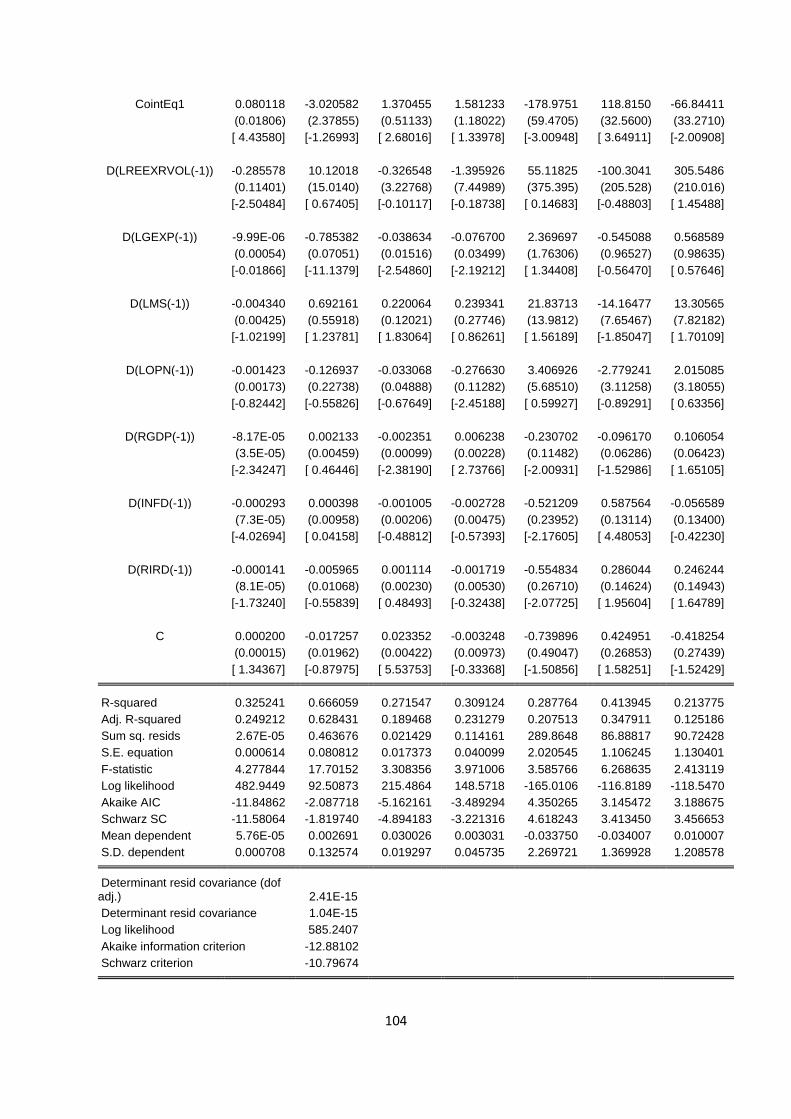
104

CointEq1 0.080118 -3.020582 1.370455 1.581233 -178.9751 118.8150 -66.84411

(0.01806) (2.37855) (0.51133) (1.18022) (59.4705) (32.5600) (33.2710)

[ 4.43580] [-1.26993] [ 2.68016] [ 1.33978] [-3.00948] [ 3.64911] [-2.00908]

D(LREEXRVOL(-1)) -0.285578 10.12018 -0.326548 -1.395926 55.11825 -100.3041 305.5486

(0.11401) (15.0140) (3.22768) (7.44989) (375.395) (205.528) (210.016)

[-2.50484] [ 0.67405] [-0.10117] [-0.18738] [ 0.14683] [-0.48803] [ 1.45488]

D(LGEXP(-1)) -9.99E-06 -0.785382 -0.038634 -0.076700 2.369697 -0.545088 0.568589

(0.00054) (0.07051) (0.01516) (0.03499) (1.76306) (0.96527) (0.98635)

[-0.01866] [-11.1379] [-2.54860] [-2.19212] [ 1.34408] [-0.56470] [ 0.57646]

D(LMS(-1)) -0.004340 0.692161 0.220064 0.239341 21.83713 -14.16477 13.30565

(0.00425) (0.55918) (0.12021) (0.27746) (13.9812) (7.65467) (7.82182)

[-1.02199] [ 1.23781] [ 1.83064] [ 0.86261] [ 1.56189] [-1.85047] [ 1.70109]

D(LOPN(-1)) -0.001423 -0.126937 -0.033068 -0.276630 3.406926 -2.779241 2.015085

(0.00173) (0.22738) (0.04888) (0.11282) (5.68510) (3.11258) (3.18055)

[-0.82442] [-0.55826] [-0.67649] [-2.45188] [ 0.59927] [-0.89291] [ 0.63356]

D(RGDP(-1)) -8.17E-05 0.002133 -0.002351 0.006238 -0.230702 -0.096170 0.106054

(3.5E-05) (0.00459) (0.00099) (0.00228) (0.11482) (0.06286) (0.06423)

[-2.34247] [ 0.46446] [-2.38190] [ 2.73766] [-2.00931] [-1.52986] [ 1.65105]

D(INFD(-1)) -0.000293 0.000398 -0.001005 -0.002728 -0.521209 0.587564 -0.056589

(7.3E-05) (0.00958) (0.00206) (0.00475) (0.23952) (0.13114) (0.13400)

[-4.02694] [ 0.04158] [-0.48812] [-0.57393] [-2.17605] [ 4.48053] [-0.42230]

D(RIRD(-1)) -0.000141 -0.005965 0.001114 -0.001719 -0.554834 0.286044 0.246244

(8.1E-05) (0.01068) (0.00230) (0.00530) (0.26710) (0.14624) (0.14943)

[-1.73240] [-0.55839] [ 0.48493] [-0.32438] [-2.07725] [ 1.95604] [ 1.64789]

C 0.000200 -0.017257 0.023352 -0.003248 -0.739896 0.424951 -0.418254

(0.00015) (0.01962) (0.00422) (0.00973) (0.49047) (0.26853) (0.27439)

[ 1.34367] [-0.87975] [ 5.53753] [-0.33368] [-1.50856] [ 1.58251] [-1.52429]

R-squared 0.325241 0.666059 0.271547 0.309124 0.287764 0.413945 0.213775

Adj. R-squared 0.249212 0.628431 0.189468 0.231279 0.207513 0.347911 0.125186

Sum sq. resids 2.67E-05 0.463676 0.021429 0.114161 289.8648 86.88817 90.72428

S.E. equation 0.000614 0.080812 0.017373 0.040099 2.020545 1.106245 1.130401

F-statistic 4.277844 17.70152 3.308356 3.971006 3.585766 6.268635 2.413119

Log likelihood 482.9449 92.50873 215.4864 148.5718 -165.0106 -116.8189 -118.5470

Akaike AIC -11.84862 -2.087718 -5.162161 -3.489294 4.350265 3.145472 3.188675

Schwarz SC -11.58064 -1.819740 -4.894183 -3.221316 4.618243 3.413450 3.456653

Mean dependent 5.76E-05 0.002691 0.030026 0.003031 -0.033750 -0.034007 0.010007

S.D. dependent 0.000708 0.132574 0.019297 0.045735 2.269721 1.369928 1.208578 Determinant resid covariance (dof

adj.) 2.41E-15

Determinant resid covariance 1.04E-15

Log likelihood 585.2407

Akaike information criterion -12.88102

Schwarz criterion -10.79674

105

Table 8.5: Vector Error Correction Estimates for Model 2 (Seven Lags)

Vector Error Correction Estimates

Date: 01/06/16 Time: 14:41



Standard errors in ( ) & t-statistics in [ ] Cointegrating Eq: CointEq1 LREEXRVOL(-1) 1.000000

LGEXP(-1) -0.034118

(0.00621)

[-5.49610]

LMS(-1) -0.002406

(0.00073)

[-3.29185]

LOPN(-1) 0.057854

(0.00585)

[ 9.88633]

RGDP(-1) -0.000996

(0.00035)

[-2.86903]

INFD(-1) 0.001151

(0.00035)

[ 3.25173]

RIRD(-1) -0.000121

(0.00021)

[-0.57946]

C -0.059330


OL) D(LGEXP) D(LMS) D(LOPN) D(RGDP) D(INFD) D(RIRD) CointEq1 0.165655 -1.228542 -3.535413 -12.25703 -186.4659 -51.10403 146.9786

(0.05871) (4.40556) (1.53059) (2.45605) (253.901) (107.662) (99.9913)

[ 2.82145] [-0.27886] [-2.30984] [-4.99054] [-0.73440] [-0.47467] [ 1.46991]

D(LREEXRVOL(-1)) -0.514558 22.76703 -0.210986 21.89749 192.8000 20.71893 62.29847

(0.20980) (15.7425) (5.46929) (8.77627) (907.270) (384.710) (357.301)

[-2.45262] [ 1.44622] [-0.03858] [ 2.49508] [ 0.21251] [ 0.05386] [ 0.17436]

D(LREEXRVOL(-2)) -0.010408 -4.356407 -1.825120 9.449344 -892.0127 204.1384 -138.6402

(0.18952) (14.2207) (4.94059) (7.92789) (819.567) (347.521) (322.762)

[-0.05492] [-0.30634] [-0.36941] [ 1.19191] [-1.08840] [ 0.58741] [-0.42954]

D(LREEXRVOL(-3)) 0.281189 29.41757 -3.450414 -5.889820 -995.7706 525.6714 -312.7149

(0.16518) (12.3945) (4.30614) (6.90982) (714.321) (302.894) (281.314)

[ 1.70231] [ 2.37343] [-0.80128] [-0.85238] [-1.39401] [ 1.73550] [-1.11162]

D(LREEXRVOL(-4)) 0.286635 -11.50307 8.107692 3.124400 -1513.366 718.8966 -409.5552

(0.17441) (13.0871) (4.54676) (7.29594) (754.237) (319.819) (297.034)

[ 1.64344] [-0.87896] [ 1.78318] [ 0.42824] [-2.00649] [ 2.24782] [-1.37882]

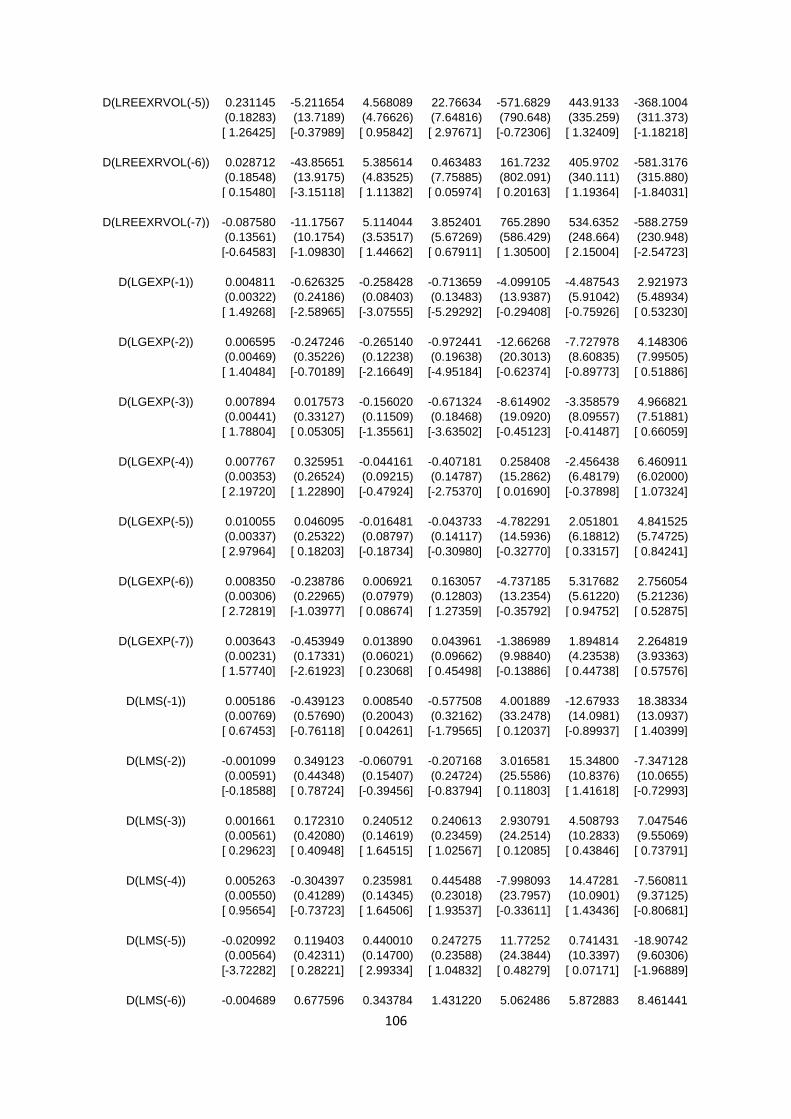
106

D(LREEXRVOL(-5)) 0.231145 -5.211654 4.568089 22.76634 -571.6829 443.9133 -368.1004

(0.18283) (13.7189) (4.76626) (7.64816) (790.648) (335.259) (311.373)

[ 1.26425] [-0.37989] [ 0.95842] [ 2.97671] [-0.72306] [ 1.32409] [-1.18218]

D(LREEXRVOL(-6)) 0.028712 -43.85651 5.385614 0.463483 161.7232 405.9702 -581.3176

(0.18548) (13.9175) (4.83525) (7.75885) (802.091) (340.111) (315.880)

[ 0.15480] [-3.15118] [ 1.11382] [ 0.05974] [ 0.20163] [ 1.19364] [-1.84031]

D(LREEXRVOL(-7)) -0.087580 -11.17567 5.114044 3.852401 765.2890 534.6352 -588.2759

(0.13561) (10.1754) (3.53517) (5.67269) (586.429) (248.664) (230.948)

[-0.64583] [-1.09830] [ 1.44662] [ 0.67911] [ 1.30500] [ 2.15004] [-2.54723]

D(LGEXP(-1)) 0.004811 -0.626325 -0.258428 -0.713659 -4.099105 -4.487543 2.921973

(0.00322) (0.24186) (0.08403) (0.13483) (13.9387) (5.91042) (5.48934)

[ 1.49268] [-2.58965] [-3.07555] [-5.29292] [-0.29408] [-0.75926] [ 0.53230]

D(LGEXP(-2)) 0.006595 -0.247246 -0.265140 -0.972441 -12.66268 -7.727978 4.148306

(0.00469) (0.35226) (0.12238) (0.19638) (20.3013) (8.60835) (7.99505)

[ 1.40484] [-0.70189] [-2.16649] [-4.95184] [-0.62374] [-0.89773] [ 0.51886]

D(LGEXP(-3)) 0.007894 0.017573 -0.156020 -0.671324 -8.614902 -3.358579 4.966821

(0.00441) (0.33127) (0.11509) (0.18468) (19.0920) (8.09557) (7.51881)

[ 1.78804] [ 0.05305] [-1.35561] [-3.63502] [-0.45123] [-0.41487] [ 0.66059]

D(LGEXP(-4)) 0.007767 0.325951 -0.044161 -0.407181 0.258408 -2.456438 6.460911

(0.00353) (0.26524) (0.09215) (0.14787) (15.2862) (6.48179) (6.02000)

[ 2.19720] [ 1.22890] [-0.47924] [-2.75370] [ 0.01690] [-0.37898] [ 1.07324]

D(LGEXP(-5)) 0.010055 0.046095 -0.016481 -0.043733 -4.782291 2.051801 4.841525

(0.00337) (0.25322) (0.08797) (0.14117) (14.5936) (6.18812) (5.74725)

[ 2.97964] [ 0.18203] [-0.18734] [-0.30980] [-0.32770] [ 0.33157] [ 0.84241]

D(LGEXP(-6)) 0.008350 -0.238786 0.006921 0.163057 -4.737185 5.317682 2.756054

(0.00306) (0.22965) (0.07979) (0.12803) (13.2354) (5.61220) (5.21236)

[ 2.72819] [-1.03977] [ 0.08674] [ 1.27359] [-0.35792] [ 0.94752] [ 0.52875]

D(LGEXP(-7)) 0.003643 -0.453949 0.013890 0.043961 -1.386989 1.894814 2.264819

(0.00231) (0.17331) (0.06021) (0.09662) (9.98840) (4.23538) (3.93363)

[ 1.57740] [-2.61923] [ 0.23068] [ 0.45498] [-0.13886] [ 0.44738] [ 0.57576]

D(LMS(-1)) 0.005186 -0.439123 0.008540 -0.577508 4.001889 -12.67933 18.38334

(0.00769) (0.57690) (0.20043) (0.32162) (33.2478) (14.0981) (13.0937)

[ 0.67453] [-0.76118] [ 0.04261] [-1.79565] [ 0.12037] [-0.89937] [ 1.40399]

D(LMS(-2)) -0.001099 0.349123 -0.060791 -0.207168 3.016581 15.34800 -7.347128

(0.00591) (0.44348) (0.15407) (0.24724) (25.5586) (10.8376) (10.0655)

[-0.18588] [ 0.78724] [-0.39456] [-0.83794] [ 0.11803] [ 1.41618] [-0.72993]

D(LMS(-3)) 0.001661 0.172310 0.240512 0.240613 2.930791 4.508793 7.047546

(0.00561) (0.42080) (0.14619) (0.23459) (24.2514) (10.2833) (9.55069)

[ 0.29623] [ 0.40948] [ 1.64515] [ 1.02567] [ 0.12085] [ 0.43846] [ 0.73791]

D(LMS(-4)) 0.005263 -0.304397 0.235981 0.445488 -7.998093 14.47281 -7.560811

(0.00550) (0.41289) (0.14345) (0.23018) (23.7957) (10.0901) (9.37125)

[ 0.95654] [-0.73723] [ 1.64506] [ 1.93537] [-0.33611] [ 1.43436] [-0.80681]

D(LMS(-5)) -0.020992 0.119403 0.440010 0.247275 11.77252 0.741431 -18.90742

(0.00564) (0.42311) (0.14700) (0.23588) (24.3844) (10.3397) (9.60306)

[-3.72282] [ 0.28221] [ 2.99334] [ 1.04832] [ 0.48279] [ 0.07171] [-1.96889]

D(LMS(-6)) -0.004689 0.677596 0.343784 1.431220 5.062486 5.872883 8.461441

107

(0.00588) (0.44137) (0.15334) (0.24606) (25.4368) (10.7860) (10.0175)

[-0.79723] [ 1.53522] [ 2.24197] [ 5.81662] [ 0.19902] [ 0.54449] [ 0.84466]

D(LMS(-7)) -0.016780 -0.333323 0.248193 0.625133 -9.452227 -4.965145 -26.66255

(0.00879) (0.65980) (0.22923) (0.36783) (38.0256) (16.1240) (14.9752)

[-1.90829] [-0.50519] [ 1.08273] [ 1.69951] [-0.24858] [-0.30794] [-1.78044]

D(LOPN(-1)) 0.000564 0.495082 -0.000154 0.126055 -3.839024 -2.776253 3.183249

(0.00328) (0.24624) (0.08555) (0.13727) (14.1910) (6.01741) (5.58871)

[ 0.17172] [ 2.01061] [-0.00180] [ 0.91828] [-0.27053] [-0.46137] [ 0.56959]

D(LOPN(-2)) 0.008787 0.157495 -0.047174 -0.257720 -29.65546 -0.906205 1.117368

(0.00259) (0.19443) (0.06755) (0.10839) (11.2052) (4.75136) (4.41285)

[ 3.39106] [ 0.81004] [-0.69837] [-2.37768] [-2.64657] [-0.19073] [ 0.25321]

D(LOPN(-3)) -0.000338 -0.314994 0.011285 -0.553607 -12.36206 -0.239311 -3.625528

(0.00312) (0.23393) (0.08127) (0.13041) (13.4817) (5.71665) (5.30937)

[-0.10829] [-1.34654] [ 0.13886] [-4.24505] [-0.91695] [-0.04186] [-0.68285]

D(LOPN(-4)) 0.009599 0.261670 -0.012593 -0.094356 -7.750276 -4.874328 9.902931

(0.00362) (0.27197) (0.09449) (0.15162) (15.6739) (6.64621) (6.17271)

[ 2.64829] [ 0.96214] [-0.13328] [-0.62233] [-0.49447] [-0.73340] [ 1.60431]

D(LOPN(-5)) 0.003668 -0.435148 -0.028254 -0.405728 -5.212017 -2.995461 -2.556017

(0.00318) (0.23862) (0.08290) (0.13303) (13.7519) (5.83124) (5.41579)

[ 1.15331] [-1.82362] [-0.34082] [-3.04998] [-0.37900] [-0.51369] [-0.47196]

D(LOPN(-6)) 0.002648 0.064429 -0.140194 -0.318897 9.345524 -5.100552 2.570157

(0.00316) (0.23747) (0.08250) (0.13239) (13.6860) (5.80329) (5.38984)

[ 0.83655] [ 0.27131] [-1.69925] [-2.40879] [ 0.68285] [-0.87891] [ 0.47685]

D(LOPN(-7)) 0.005324 -0.095297 -0.062603 -0.231720 5.312590 -8.266154 7.604983

(0.00277) (0.20759) (0.07212) (0.11573) (11.9636) (5.07294) (4.71152)

[ 1.92462] [-0.45907] [-0.86804] [-2.00229] [ 0.44406] [-1.62946] [ 1.61413]

D(RGDP(-1)) 0.000159 -0.004851 -0.005532 -0.007674 -0.886944 -0.109546 0.111224

(7.4E-05) (0.00556) (0.00193) (0.00310) (0.32056) (0.13593) (0.12624)

[ 2.14040] [-0.87204] [-2.86277] [-2.47473] [-2.76682] [-0.80591] [ 0.88102]

D(RGDP(-2)) 0.000132 -0.016092 -0.002064 -0.013164 -0.444455 -0.080388 0.086687

(8.9E-05) (0.00665) (0.00231) (0.00371) (0.38328) (0.16252) (0.15094)

[ 1.48656] [-2.41964] [-0.89341] [-3.55056] [-1.15961] [-0.49463] [ 0.57430]

D(RGDP(-3)) 0.000164 -0.003640 -0.001124 -0.009143 -0.324330 -0.057451 -0.007314

(8.1E-05) (0.00606) (0.00211) (0.00338) (0.34939) (0.14815) (0.13759)

[ 2.02933] [-0.60047] [-0.53388] [-2.70522] [-0.92829] [-0.38779] [-0.05316]

D(RGDP(-4)) 0.000316 -0.000751 -0.001649 -0.008989 -0.424523 0.040861 -0.005155

(7.5E-05) (0.00563) (0.00196) (0.00314) (0.32441) (0.13756) (0.12776)

[ 4.21229] [-0.13350] [-0.84308] [-2.86437] [-1.30860] [ 0.29704] [-0.04035]

D(RGDP(-5)) 0.000137 -0.012025 -0.000952 -0.002489 -0.323401 0.033690 -0.023651

(7.7E-05) (0.00581) (0.00202) (0.00324) (0.33466) (0.14190) (0.13179)

[ 1.76622] [-2.07077] [-0.47209] [-0.76884] [-0.96636] [ 0.23742] [-0.17946]

D(RGDP(-6)) 7.10E-05 -0.008038 0.000363 -0.000823 0.053218 -0.050955 -0.074551

(6.2E-05) (0.00465) (0.00161) (0.00259) (0.26787) (0.11358) (0.10549)

[ 1.14600] [-1.72935] [ 0.22464] [-0.31776] [ 0.19867] [-0.44861] [-0.70670]

D(RGDP(-7)) 5.50E-05 -0.014406 0.000327 0.003478 0.047767 -0.017642 -0.024894

(5.2E-05) (0.00391) (0.00136) (0.00218) (0.22554) (0.09563) (0.08882)

108

[ 1.05407] [-3.68131] [ 0.24054] [ 1.59396] [ 0.21179] [-0.18447] [-0.28027]

D(INFD(-1)) -0.000498 0.001525 0.003497 0.013172 -0.036336 0.410850 0.124842

(0.00013) (0.00986) (0.00343) (0.00550) (0.56853) (0.24107) (0.22390)

[-3.78630] [ 0.15460] [ 1.02024] [ 2.39516] [-0.06391] [ 1.70425] [ 0.55758]

D(INFD(-2)) -0.000485 0.005434 0.000955 0.017874 0.753138 -0.120124 -0.443116

(0.00019) (0.01449) (0.00503) (0.00808) (0.83500) (0.35407) (0.32884)

[-2.51195] [ 0.37505] [ 0.18980] [ 2.21294] [ 0.90196] [-0.33927] [-1.34751]

D(INFD(-3)) 7.60E-05 -0.004519 0.002855 0.000876 -0.823697 0.078038 0.220065

(0.00016) (0.01197) (0.00416) (0.00667) (0.68999) (0.29257) (0.27173)

[ 0.47651] [-0.37749] [ 0.68639] [ 0.13130] [-1.19379] [ 0.26673] [ 0.80986]

D(INFD(-4)) -8.69E-05 0.038757 -0.008195 0.011596 -5.19E-06 -0.924217 0.324235

(0.00017) (0.01289) (0.00448) (0.00718) (0.74273) (0.31494) (0.29250)

[-0.50604] [ 3.00733] [-1.83032] [ 1.61405] [-7.0e-06] [-2.93460] [ 1.10849]

D(INFD(-5)) -0.000163 -0.025743 0.012737 -0.008975 -0.224346 0.556990 -0.196740

(0.00020) (0.01514) (0.00526) (0.00844) (0.87255) (0.36999) (0.34363)

[-0.80719] [-1.70031] [ 2.42149] [-1.06333] [-0.25712] [ 1.50544] [-0.57254]

D(INFD(-6)) -0.000254 0.018600 -0.007994 0.022121 -0.001879 -0.141214 0.092435

(0.00024) (0.01815) (0.00631) (0.01012) (1.04603) (0.44355) (0.41195)

[-1.04980] [ 1.02477] [-1.26772] [ 2.18616] [-0.00180] [-0.31838] [ 0.22438]

D(INFD(-7)) 0.000393 -0.017809 -0.006873 -0.021443 -0.746966 0.107949 -0.171278

(0.00019) (0.01439) (0.00500) (0.00802) (0.82906) (0.35154) (0.32650)

[ 2.05010] [-1.23796] [-1.37515] [-2.67379] [-0.90098] [ 0.30707] [-0.52459]

D(RIRD(-1)) -1.94E-05 -0.002311 0.008574 0.008327 -0.610592 0.106830 0.790203

(0.00015) (0.01105) (0.00384) (0.00616) (0.63684) (0.27004) (0.25080)

[-0.13178] [-0.20916] [ 2.23338] [ 1.35178] [-0.95878] [ 0.39561] [ 3.15072]

D(RIRD(-2)) -0.000498 0.003998 -0.005452 0.020309 1.018823 0.018133 -0.970867

(0.00022) (0.01629) (0.00566) (0.00908) (0.93909) (0.39820) (0.36983)

[-2.29145] [ 0.24537] [-0.96312] [ 2.23573] [ 1.08491] [ 0.04554] [-2.62516]

D(RIRD(-3)) -0.000128 -0.019616 0.011680 -0.000802 -0.361437 -0.051368 0.546619

(0.00019) (0.01463) (0.00508) (0.00815) (0.84298) (0.35745) (0.33198)

[-0.65525] [-1.34107] [ 2.29838] [-0.09839] [-0.42876] [-0.14371] [ 1.64654]

D(RIRD(-4)) -0.000248 0.047553 -0.014315 0.014486 0.539539 -0.409694 -0.244581

(0.00023) (0.01741) (0.00605) (0.00971) (1.00366) (0.42558) (0.39526)

[-1.06964] [ 2.73058] [-2.36594] [ 1.49207] [ 0.53757] [-0.96267] [-0.61878]

D(RIRD(-5)) -4.79E-05 -0.027342 0.012372 -0.018502 -0.783428 0.198038 0.334711

(0.00025) (0.01859) (0.00646) (0.01036) (1.07111) (0.45418) (0.42183)

[-0.19335] [-1.47117] [ 1.91599] [-1.78573] [-0.73142] [ 0.43603] [ 0.79348]

D(RIRD(-6)) -0.000179 0.026710 -0.014084 0.020758 -0.293085 0.056142 -0.176768

(0.00026) (0.01936) (0.00673) (0.01080) (1.11596) (0.47320) (0.43949)

[-0.69493] [ 1.37937] [-2.09360] [ 1.92294] [-0.26263] [ 0.11864] [-0.40221]

D(RIRD(-7)) 0.000345 -0.018015 -0.004444 -0.023821 -1.056597 -0.060498 0.009949

(0.00022) (0.01622) (0.00564) (0.00904) (0.93488) (0.39642) (0.36818)

[ 1.59708] [-1.11055] [-0.78848] [-2.63404] [-1.13019] [-0.15261] [ 0.02702]

C 0.000875 -0.006734 -0.014879 -0.061562 -0.204410 -0.749283 0.781291

(0.00032) (0.02434) (0.00846) (0.01357) (1.40265) (0.59476) (0.55239)

[ 2.69634] [-0.27667] [-1.75970] [-4.53726] [-0.14573] [-1.25980] [ 1.41438]

109

R-squared 0.854991 0.973964 0.860402 0.928022 0.703910 0.864226 0.834116

Adj. R-squared 0.539756 0.917362 0.556927 0.771549 0.060237 0.569066 0.473500

Sum sq. resids 5.67E-06 0.031904 0.003851 0.009915 105.9660 19.05284 16.43473

S.E. equation 0.000496 0.037244 0.012939 0.020763 2.146443 0.910156 0.845313

F-statistic 2.712228 17.20752 2.835166 5.930868 1.093584 2.927993 2.313028

Log likelihood 501.2448 181.7153 259.9491 224.9543 -118.2864 -54.79805 -49.32872

Akaike AIC -12.16878 -3.532845 -5.647273 -4.701468 4.575308 2.859407 2.711587

Schwarz SC -10.58084 -1.944908 -4.059336 -3.113531 6.163245 4.447343 4.299524

Mean dependent 3.55E-05 0.001297 0.029115 0.001932 -0.048649 0.016115 -0.085034

S.D. dependent 0.000732 0.129559 0.019439 0.043441 2.214166 1.386471 1.164979 Determinant resid covariance (dof

adj.) 1.05E-17

Determinant resid covariance 2.94E-21

Log likelihood 1014.189

Akaike information criterion -17.57266

Schwarz criterion -6.239153

Table 8.6: Variance Decomposition Analysis for Model One (One Lag)

Period S.E. LREEXRVOL LGEXP LMS LOPN RGDP INFD RIRD 1 0.000614 100.0000 0.000000 0.000000 0.000000 0.000000 0.000000 0.000000

2 0.000832 87.01091 0.402417 0.801259 0.127125 0.741438 7.987984 2.928867

3 0.001046 73.69584 0.282220 0.519606 0.611111 3.756456 12.78995 8.344818

4 0.001244 62.08091 0.272831 0.437518 0.705738 4.507561 17.39914 14.59630

5 0.001428 53.61248 0.207951 0.444931 0.727216 4.894919 20.48958 19.62293

6 0.001596 47.66699 0.176713 0.441525 0.717584 4.927535 22.69688 23.37278

7 0.001748 43.51861 0.147474 0.441790 0.687627 4.865253 24.21817 26.12108

8 0.001886 40.59717 0.128040 0.427100 0.660001 4.733620 25.35006 28.10401

9 0.002013 38.49314 0.112838 0.413538 0.631315 4.608658 26.17696 29.56355

10 0.002130 36.94616 0.101001 0.395693 0.607956 4.479664 26.82549 30.64404

11 0.002239 35.77291 0.091609 0.380444 0.586585 4.371324 27.32700 31.47014

12 0.002342 34.86039 0.083766 0.364934 0.569376 4.271538 27.73889 32.11110

13 0.002441 34.12694 0.077257 0.351976 0.554077 4.189263 28.07349 32.62699

14 0.002535 33.52345 0.071654 0.339765 0.541583 4.115700 28.35886 33.04899

15 0.002625 33.01311 0.066835 0.329547 0.530479 4.054496 28.59994 33.40559

16 0.002712 32.57433 0.062612 0.320156 0.521194 3.999873 28.81132 33.71052

17 0.002797 32.18996 0.058894 0.312193 0.512863 3.953498 28.99505 33.97754

18 0.002879 31.85000 0.055590 0.304910 0.505716 3.911751 29.15919 34.21284

19 0.002959 31.54580 0.052634 0.298619 0.499229 3.875493 29.30474 34.42349

20 0.003037 31.27216 0.049977 0.292847 0.493535 3.842504 29.43640 34.61258

21 0.003112 31.02415 0.047573 0.287763 0.488318 3.813267 29.55483 34.78410

22 0.003186 30.79865 0.045390 0.283074 0.483656 3.786425 29.66294 34.93987

23 0.003259 30.59251 0.043397 0.278874 0.479353 3.762255 29.76122 35.08239

24 0.003330 30.40359 0.041572 0.274980 0.475455 3.739913 29.85157 35.21292

25 0.003399 30.22971 0.039894 0.271445 0.471839 3.719550 29.93442 35.33315

26 0.003467 30.06930 0.038346 0.268153 0.468529 3.700631 30.01104 35.44401

27 0.003533 29.92078 0.036914 0.265133 0.465445 3.683229 30.08180 35.54670

28 0.003599 29.78299 0.035585 0.262310 0.462598 3.666992 30.14758 35.64195

29 0.003663 29.65473 0.034348 0.259700 0.459937 3.651948 30.20870 35.73064

30 0.003726 29.53512 0.033194 0.257251 0.457463 3.637859 30.26578 35.81333

31 0.003788 29.42327 0.032115 0.254972 0.455143 3.624726 30.31910 35.89067

32 0.003849 29.31848 0.031104 0.252828 0.452974 3.612387 30.36911 35.96312

33 0.003909 29.22007 0.030155 0.250821 0.450933 3.600825 30.41603 36.03116

34 0.003969 29.12751 0.029262 0.248928 0.449017 3.589928 30.46020 36.09516

35 0.004027 29.04026 0.028421 0.247148 0.447207 3.579673 30.50180 36.15549

36 0.004084 28.95790 0.027626 0.245464 0.445502 3.569979 30.54110 36.21243

determinants of exchange rate volatility in south africa

Documents