Economic Research Southern Africa (ERSA) is a research programme funded by the National

Treasury of South Africa. The views expressed are those of the author(s) and do not necessarily represent those of the funder, ERSA or the author’s affiliated

institution(s). ERSA shall not be liable to any person for inaccurate information or opinions contained herein.

The Determinants of Exchange Rate

Volatility in South Africa

Trust Mpofu

ERSA working paper 604

May 2016

The Determinants of Exchange RateVolatility in South Africa�

Trust R. Mpofuy

University of Cape Town

April 14, 2016

Abstract

This paper investigates the determinants of exchange rate volatil-ity in South Africa for the period 1986�2013 using the New OpenEconomy Macroeconomics model by Obstfeld & Rogo¤ (1996) andHau (2002). The main focus of the paper is to test the hypothesisthat economic openness decreases Rand (ZAR) volatility. This followsSouth Africa�s liberalisation of its capital account in the mid-1990sand the mixed results in the literature on the relationship betweenexchange rate volatility and economic openness. Employing monthlytime series data, GARCH models are estimated. The study �nds thatswitching to a �oating exchange rate regime has a signi�cant positivee¤ect on ZAR volatility. The results also indicate that trade open-ness signi�cantly reduces ZAR volatility only when bilateral exchangerates are used, but �nds the opposite when multilateral exchange ratesare used. The study also �nds that volatility of output, commodityprices, money supply and foreign reserves signi�cantly in�uence ZARvolatility.Keywords: Exchange Rate Volatility, GARCH.JEL Classi�cation: F31, C22

�I would like to thank the session participants at the 17th Annual INFER conference inLuton, UK 2015 and the Econometric Society, Africa Region Training workshop in Lusaka,Zambia 2015 for their constructive comments and suggestions. I also bene�tted from thecomments and suggestions of an anonymous referee.

ySchool of Economics, University of Cape Town, South Africa. Email: trustm-pofu@gmail.com

1

1 Introduction

Increasing �nancial liberalisation since the collapse of the Bretton Woodssystem in the 1970s has rendered exchange rates volatile in both developedand developing countries. As a result, the causes and e¤ects of exchangerate volatility have become of particular interest to both researchers andpolicymakers. South Africa liberalised its capital account in March 1995following the abolishment of the dual exchange rate system which had been inplace since the mid-1980s. The South African currency (the Rand, henceforthZAR) has subsequently been more volatile (Arezki, Dumitrescu, Freytag &Quintyn 2014, Ricci 2005). But, one might ask, why study the performance ofthe ZAR? The answer is that the ZAR is one of the most important emergingmarket currencies according to the 2013 survey by the Bank for InternationalSettlements (BIS) (see table 1).

< Insert Table 1 Here>Given the above, the question that follows is, did economic openness

in March 1995 increase ZAR volatility? This follows �ndings by empiricalstudies. Some researchers �nd that economic openness reduces exchangerate volatility (Hau 2002, Calderón 2004, Bleaney 2008), while others �ndthe opposite or no relationship (Amor & Sarkar 2008, Caporale, Amor &Rault 2009, Grydaki & Fountas 2010, Chipili 2012, Jabeen & Khan 2014).Due to con�icting results in empirical studies, only an empirical analysiscan show the relationship between exchange rate volatility and economicopenness in a country which has experienced an institutional change in itsexchange rate regime. As such, this paper follows the modi�ed version of theNew Open Economy Macroeconomics model of Obstfeld & Rogo¤ (1996) byHau (2002). This theoretical model asserts that there should be a negativerelationship between exchange rate volatility and economic openness. Thatis, more open economies should have less exchange rate volatility. This studyalso tests the hypothesis that economic openness decreases ZAR volatility.Few studies investigate the determinants of ZAR volatility. Arezki et al.

(2014) examine the relationship between ZAR volatility and gold price volatil-ity. Farrell (2001) analyses whether the imposition of capital controls in themid-1980s a¤ected commercial ZAR variability di¤erently to �nancial ZARvariability between 1985 and 1995. This paper contributes to the literature by�nding the sources of ZAR volatility using output volatility, money supplyvolatility, foreign reserves�volatility, commodity price volatility, openness,and a dummy for capital account liberalisation, as explanatory variables.Several factors motivate this study. Firstly, many variables in�uence

the level of the ZAR (Aron, Elbadawi & Kahn 1997, MacDonald & Ricci2004, Frankel 2007, Saayman 2007, Faulkner & Makrelov 2008). Many vari-

2

ables might also cause large swings in the exchange rates. Secondly, ex-change rate volatility is important in macroeconomics literature. In SouthAfrica there is evidence of exchange rate volatility having signi�cant ef-fect on macroeconomic factors such as employment and trade (Todani &Munyama 2005, Mpofu 2013, Aye, Gupta, Moyo & Pillay 2014). Finding thesources of exchange rate volatility is relevant to policymakers and researchersto assist them to investigate how to tackle some of the e¤ects of exchangerate volatility.Thirdly, studies by Hau (2002) and Calderón (2004) attempt to �nd the

sources of exchange rate volatility in South Africa1. However, these studiesuse cross-country data and �nd aggregate results which do not isolate coun-try speci�c e¤ects. Besides, Hau (2002) states that the theoretical linkagebetween openness and real exchange rate volatility depends on the magni-tude of the monetary and real shocks of each country. This suggests thatanalysing the sources of exchange rate volatility at a country level will likelybe better for formulation of the correct type of policy response(s). Further-more, they measure exchange rate volatility using very low frequency data(i.e. yearly data) yet exchange rate volatility will be best measured usingeither very high frequency data (i.e. intraday or daily data) or low frequencydata (i.e. monthly or quarterly data).Fourthly, the ZAR is indeed volatile. Using simple standard deviations of

log real exchange rate of the domestic currency per United States dollar, table2 shows the volatility of the ZAR compared to selected emerging markets.This table indicates that the ZAR is on average more volatile than the Indian,South Korean and Russian currencies but less volatile than Turkish, Brazilianand Malaysian currencies for the period 1992 � 20132.

<Insert Table 2 Here>Using GARCHmodels for the period 1986 to 2013 and employing monthly

data, the study �nds that switching to a �oating exchange rate regime in-creases exchange rate volatility, trade openness reduces exchange rate volatil-ity using the bilateral exchange rate of ZAR/US dollar while the oppositeis found when using e¤ective exchange rate. The results suggest that tradewith some of South Africa�s trading partners is less open. The results alsoshow that volatility of output, commodity prices, money supply, and foreignreserves signi�cantly in�uence ZAR volatility.The structure of the paper is as follows: section 2 presents the literature

1This follows the fact that South Africa is included in their sample of countries analysed.2This shorter period is chosen due to lack of data for some variables used when calcu-

lating the real exchange rate prior to 1992M7. Here Real Exchange Rate is calculated asNominal exchange rate * CPI�

CPI where CPI� is the foreign price and CPI is the domesticprice.

3

review. Section 3 presents the theoretical model of exchange rate volatility.Section 4 reports the data and the descriptive statistics of the data used.Section 5 presents the econometric approach used, while section 6 reportsempirical results. Section 7 provides the conclusion.

2 Literature Review

There is no general consensus on the macroeconomic determinants of ex-change rate volatility in the literature. This is due to di¤erent approachesused based on di¤erent theoretical models of exchange rate level determina-tion. Some studies examine the sources of exchange rate volatility using aspeci�c exchange rate level model, whilst others are based on a synthesis ofexchange rate level models.Examples of speci�c models are as follows. First are studies based on the

monetary models of exchange rate level determination (Morana 2009, Gry-daki & Fountas 2009, Grydaki & Fountas 2010). These studies emphasisemonetary variables as the determinants of exchange rate volatility. Secondis the Optimum Currency Areas�model (Bayoumi & Eichengreen 1998, De-vereux & Lane 2003). These studies put emphasis on trade linkages; asym-metry or similarity of economic shocks to output, country size and geo-graphic factors, as the determinants of exchange rate volatility. Third isthe New Open Economy Macroeconomics (Hau 2002, Calderón 2004, Amor& Sarkar 2008, Caporale et al. 2009). These studies stress that monetaryvariables and non-monetary factors are important in explaining exchangerate volatility.Research which synthesises exchange rate models include studies by Chip-

ili (2012) and Jabeen & Khan (2014) to mention a few. These studies usevariables from di¤erent speci�c models considered important in explainingexchange rate movements in the countries of their studies. However, otherstudies �nd no link between macroeconomic fundamentals and exchangerate volatility (Flood & Rose 1995). Such studies support the role of non-macroeconomic determinants of exchange rate volatility. For example, mi-crostructure factors like the aggregation of a large number of news sources(Morana 2009 who cites Andersen & Bollerslev 1997).Of the di¤erent models used for �nding the determinants of exchange rate

volatility above, this study uses the New Open Economy Macroeconomicsmodel. This is due to the opening up of the �nancial system in South Africato the rest of the world in March 1995. Prior to March 1995, South Africahad followed a dual exchange rate system from September 1985 to March1995. During this period, the foreign exchange transactions of non-resident

4

portfolio investors on the capital account was separate from all other foreignexchange transactions3. This was the result of the increased volatility ofthe South African ZAR during the period 1982 to 1985 because of politicalpressure from the international community, which imposed trade sanctionsbecause of Apartheid. The uni�cation of the �nancial and commercial ZARsystems of capital controls in March 1995 make the use of New Open Econ-omy Macroeconomics model appropriate to investigate the impact of sucha change in institutional settings on the relationship between exchange ratevolatility and its fundamentals. Subsequent studies discussed in the empiricalliterature �nd the following:Arezki et al. (2014) employs a Vector Error Correction Model (VECM)

to examine the relationship between the South African ZAR and gold pricevolatility for the period 1980 � 2010, using monthly data. Their resultsindicate that gold price volatility is vital in explaining the excessive exchangerate volatility of the ZAR. However, their paper only used commodity priceswhich do not capture a larger set of fundamental relative price movements.This paper contributes to this literature by using more explanatory variablesfor the determinants of South African ZAR volatility. In addition, this papercontributes to the debate about exchange rates in South Africa by focusingon the determinants of exchange rate volatility (i.e. the second moment ofthe relationship between the exchange rate and its determinants) given thatmost studies in South Africa have analysed the determinants of the levelof the exchange rate (i.e. the �rst moment of the relationship between theexchange rate and its determinants) (see e.g. Aron et al. 1997, MacDonald& Ricci 2004, Frankel 2007, Saayman 2007, Faulkner & Makrelov 2008).Hau (2002) employs cross-sectional analysis on 48 (23 OECD and 25

non-OECD) countries over the period 1980 - 1998. He uses annual dataon real e¤ective exchange rate (REER) volatility measured as the movingsample standard deviation of REER percentage changes over three-year pe-riod. With control variables of per capita GDP, dummies for revolutions andcoups, central bank independence, and exchange rate commitments, Hau�nds a negative relationship between real exchange rate volatility and tradeopenness. That is, more open economies will have less real exchange ratevolatility. The theoretical linkage between real exchange rate volatility andopenness depends on the magnitude of monetary and real shocks of eachcountry. Hau (2002) therefore re-estimates the regression equation usingonly OECD countries, given that they are more homogeneous4. He still �nds

3The �nancial ZAR system of capital controls was imposed on non-resident portfolioinvestors while the other was the commercial ZAR system.

4This is based on the notion that these countries experience similar shocks which arerelatively of the same magnitude.

5

a negative relationship between real exchange rate volatility and trade open-ness, but the results are more pronounced (they have higher explanatorypower) than the results using 48 countries.Calderón (2004) uses a GMM method on 77 industrial and developing

countries over the period 1974 - 2003. Calderon uses annual data on REERvolatility measured as the standard deviation of changes in the REER overa 5-year period, as well as the volatility of real exchange rate fundamen-tals. Calderón (2004) �nds that there is a negative relationship between realexchange rate volatility and economic openness. He also �nds a negativerelationship between real exchange rate volatility and government spendingvolatility. He, however, �nds a positive relationship between real exchangerate volatility and output, money supply, and terms of trade volatilities re-spectively. Using the same GMM method, Amor & Sarkar (2008) also �nd anegative relationship between exchange rate volatility and trade openness forten South and South East Asia economies. Bleaney (2008) also �nds similarresults for real exchange rate volatility and trade openness.Caporale et al. (2009) �nd a similar negative relationship between real

exchange rate volatility and trade openness for the period 1979 - 2004. Theirresults show that there is a positive relationship between real exchange ratevolatility and �nancial openness for the entire sample, which comprises 39developing countries (20 from Latin America, ten from Asia, and nine fromMENA5). These results are similar to Amor & Sarkar (2008). However, theregressions for the three separate regions �nd di¤erent results. For the Asianregion, they �nd that �nancial openness causes real exchange rates to bemore volatile, but REER volatility is mainly due to domestic real shocks,while external shocks play a small role. For the MENA region, they �ndthat �nancial openness causes the real exchange rate to be less volatile, butREER volatility is mainly caused by monetary and real shocks. For theLatin American region, they �nd that external and monetary shocks are themain sources of real exchange rate volatility. The results by Hau (2002) forOECD countries only and the analysis by Caporale et al. (2009) suggestthat �nding the sources of exchange rate volatility for a single country ismore appropriate for policymakers because the results are not generalised.This study also improves on studies that use standard deviation as the proxyfor volatility, because GARCH models are able to describe the time-varyingvolatility directly which the standard deviation models are unable to do.Using daily data from 1 January 1999 to 31 December 2004, (Stanc¬k 2006,

Stanc¬k 2007) investigates the determinants of real exchange rate volatility

5The countries in the MENA region include: Algeria, Egypt, Iran, Israel, Jordan,Morocco, Syria, Tunisia and Turkey.

6

for six Central and Eastern European countries. The study focuses on tradeopenness, news factors, and exchange rate regimes as explanatory variables.Real exchange rate used is the bilateral between the Euro and the U.S. dollar.Real exchange rate volatility is measured using the threshold autoregressiveconditional heteroskedasticity (TARCH) model. The �nal model is estimatedusing Ordinary Least Squares (OLS) and the results for each country indicatethat there is a negative relationship between real exchange rate volatility andtrade openness for the four countries. The other two countries show insignif-icant coe¢ cients between real exchange rate volatility and trade openness.The news factor presents mixed results for di¤erent countries.Chipili (2012) examines the sources of volatility of the Zambian kwacha

exchange rate (real and nominal) using the GARCHmodels (GARCH, TARCHand EGARCH). He �nds that both monetary factors (money supply, in�a-tion, short-term domestic interest rate, and foreign reserves), and real factors(terms of trade, openness, and output) a¤ect exchange rate volatility. The re-sults indicate that real factors have smaller e¤ects on exchange rate volatilitythan monetary factors. This suggest that monetary policy has an importantrole in mitigating the volatility of the exchange rate. His results show thatusing the GARCH(1,1) and TARCH(1,1) models, the relationship betweenexchange rate volatility and openness is insigni�cant. Using an EGARCHmodel, he �nds a positive and signi�cant relationship between exchange ratevolatility and openness for the kwacha and 19 other currencies, except forZimbabwean dollar, which is negative and signi�cant. He asserts that thedi¤erent �ndings regarding openness for some exchange rate volatility sug-gest that the degree of openness, that is, the extent of trade linkages betweenZambia and her trading partners, is low relative to what is implied by theory.Jabeen & Khan (2014) also use various macroeconomic factors to �nd the

determinants of exchange rate volatility in Pakistan using GARCH(1,1) andTARCH(1,1) models. Their study �nds that real output volatility, foreignexchange reserves�volatility, in�ation volatility, productivity, and terms oftrade volatility are important determinants of exchange rate volatility. Theirstudy uses trade restrictions measured by the reciprocal of trade opennessand the results �nd positive and insigni�cant coe¢ cients for this variable.Morana (2009) also �nds support for macroeconomic fundamentals in in�u-encing exchange rate volatility. Morana (2009) argues that the exchangerate is an important determinant of aggregate demand, and therefore con-ducts the Granger-Causality test to establish the direction of causality. Theresults show that causality is bi-directional, but is stronger from macroeco-nomic factors to exchange rate volatility than vice-versa. This suggest thatstability in the macroeconomic variables is recommended to reduce exchangerate volatility, which contradicts the �ndings of Flood & Rose (1995) in their

7

study for G-7 countries.

3 Theoretical Model

This paper uses the New Open Economy Macroeconomics (NOEM) model asthe theoretical framework linking exchange rate volatility, economic opennessand the volatility of exchange rate fundamentals. The NOEMmodel is basedon the work of Obstfeld & Rogo¤ (1996) which formalises exchange ratedetermination in the context of dynamic general equilibrium models withexplicit microfoundation, imperfect competition, and nominal rigidities.The NOEM model is ideal for measuring economic openness and the

volatility of exchange rate fundamentals of South Africa for the followingreasons: First, South Africa is a good case study following the liberalisationof the capital account in March 1995. Such institutional change in the ex-change rate regime enables one to test the hypothesis that economic opennessleads to a reduction in exchange rate volatility, as asserted by Hau (2002),and investigate the relationship between exchange rate volatility and its fun-damentals.Secondly, this model emphasises that both monetary and non-monetary

variables are important in explaining exchange rate volatility. This is unlikemodels based only on exchange rate determination using monetary or opti-mum currency areas. Monetary variables might matter in South Africa intrying to explain the ZAR volatility because the ZAR is volatile while at thesame time the monetary authorities have not been able to stabilise in�ationrates at low levels. This follows arguments by Dornbusch (1976) and Rogo¤(1999). Dornbusch�s (1976) overshooting model shows that monetary policyshocks might lead to disproportionately large �uctuations in exchange rates.Dornbusch�s (1976) model asserts that monetary instability can lead to ex-cessive exchange rate instability, thus putting the blame for exchange ratevolatility on monetary authorities.However, Rogo¤ (1999) argues that monetary authorities cannot take

the blame for causing exchange rate volatility, as most industrial economieshave stabilised in�ation rates6 and their exchange rates are still signi�cantlyvolatile. Although South Africa is categorised as an emerging market econ-omy, its �nancial sector is well developed. At the same time, its in�ationrate has not fallen and stabilised at low levels. This supports the use ofmonetary variables as explanatory variables for exchange rate volatility inSouth Africa.

6The countries in question are the U.S.A, Japan and European countries where thein�ation rates stabilised at rates below 3 percent.

8

Other studies in South Africa (Aron et al. 1997, MacDonald & Ricci 2004,Frankel 2007, Saayman 2007, Faulkner & Makrelov 2008) show that non-monetary factors signi�cantly in�uence the level of the ZAR. This �nding,together with arguments by Meese & Rogo¤(1983) that monetary models areunable to replicate and forecast exchange rate swings, imply that monetaryvariables are only one of several factors driving exchange rate volatility. Thusthe literature that uses the NOEM model argues that non-monetary factorshave gained importance in explaining exchange rate volatility.To show the link between exchange rate volatility, economic openness,

and the volatility of exchange rate fundamentals, this study follows the workof Obstfeld & Rogo¤(1996) and Hau (2002)7. Using the �rst order conditionsderived from the basic set up of the model, trade openness is de�ned as

Openness =PTCT

PNCN + PTCT= ' (1)

Following this de�nition, the dynamics of the model are analysed takingthe log-linear approximation from the initial steady state. The temporary

percentage change from the initial steady state is denoted by X =(X1�X0)

X0while the permanent percentage change from the initial steady state is de-

noted by X =(X�X0)X0

:The model �rst analyses monetary shocks. The model assumes that the

economy encounters an unanticipated permanent monetary shock, that is,MS = MS. This assumption and log-linearizing equation 29 around thesteady state results in the following equation:

" (m� p) = pT � p+�

1� � (pT � p) (2)

Given that the prices of nontradables are �xed in the short-run, that is,PN = 0 and the long-run neutrality of money, PT =MS leads to:

PT =� + (1� �) "

� + (1� �) (1� '+ '")MS (3)

Since the law of one price holds for tradables, the short-run percentageprice change is proportional to money supply and exchange rate. That is,PT = M

S = E: Given that consumption smoothing implies a constant con-sumption of tradables, it then means CT = 0: Following this and the nominalrigid nontradables�prices implies that the real price of nontradables decreases

7See the appendix for the detailed explanation of the basic set up and steady stateanalysis of the model.

9

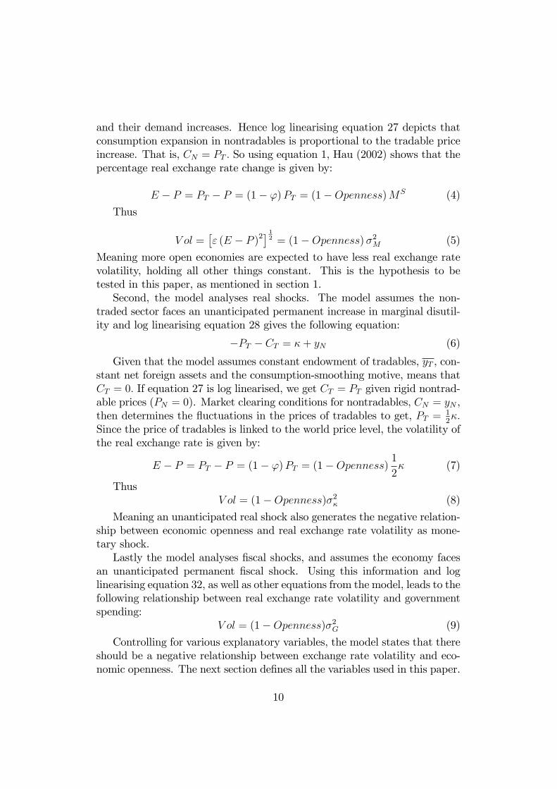
and their demand increases. Hence log linearising equation 27 depicts thatconsumption expansion in nontradables is proportional to the tradable priceincrease. That is, CN = PT : So using equation 1, Hau (2002) shows that thepercentage real exchange rate change is given by:

E � P = PT � P = (1� ')PT = (1�Openness)MS (4)

Thus

V ol =�" (E � P )2

� 12 = (1�Openness)�2M (5)

Meaning more open economies are expected to have less real exchange ratevolatility, holding all other things constant. This is the hypothesis to betested in this paper, as mentioned in section 1.Second, the model analyses real shocks. The model assumes the non-

traded sector faces an unanticipated permanent increase in marginal disutil-ity and log linearising equation 28 gives the following equation:

�PT � CT = �+ yN (6)

Given that the model assumes constant endowment of tradables, yT , con-stant net foreign assets and the consumption-smoothing motive, means thatCT = 0: If equation 27 is log linearised, we get CT = PT given rigid nontrad-able prices (PN = 0). Market clearing conditions for nontradables, CN = yN ,then determines the �uctuations in the prices of tradables to get, PT = 1

2�:

Since the price of tradables is linked to the world price level, the volatility ofthe real exchange rate is given by:

E � P = PT � P = (1� ')PT = (1�Openness)1

2� (7)

ThusV ol = (1�Openness)�2� (8)

Meaning an unanticipated real shock also generates the negative relation-ship between economic openness and real exchange rate volatility as mone-tary shock.Lastly the model analyses �scal shocks, and assumes the economy faces

an unanticipated permanent �scal shock. Using this information and loglinearising equation 32, as well as other equations from the model, leads to thefollowing relationship between real exchange rate volatility and governmentspending:

V ol = (1�Openness)�2G (9)

Controlling for various explanatory variables, the model states that thereshould be a negative relationship between exchange rate volatility and eco-nomic openness. The next section de�nes all the variables used in this paper.

10

4 Data

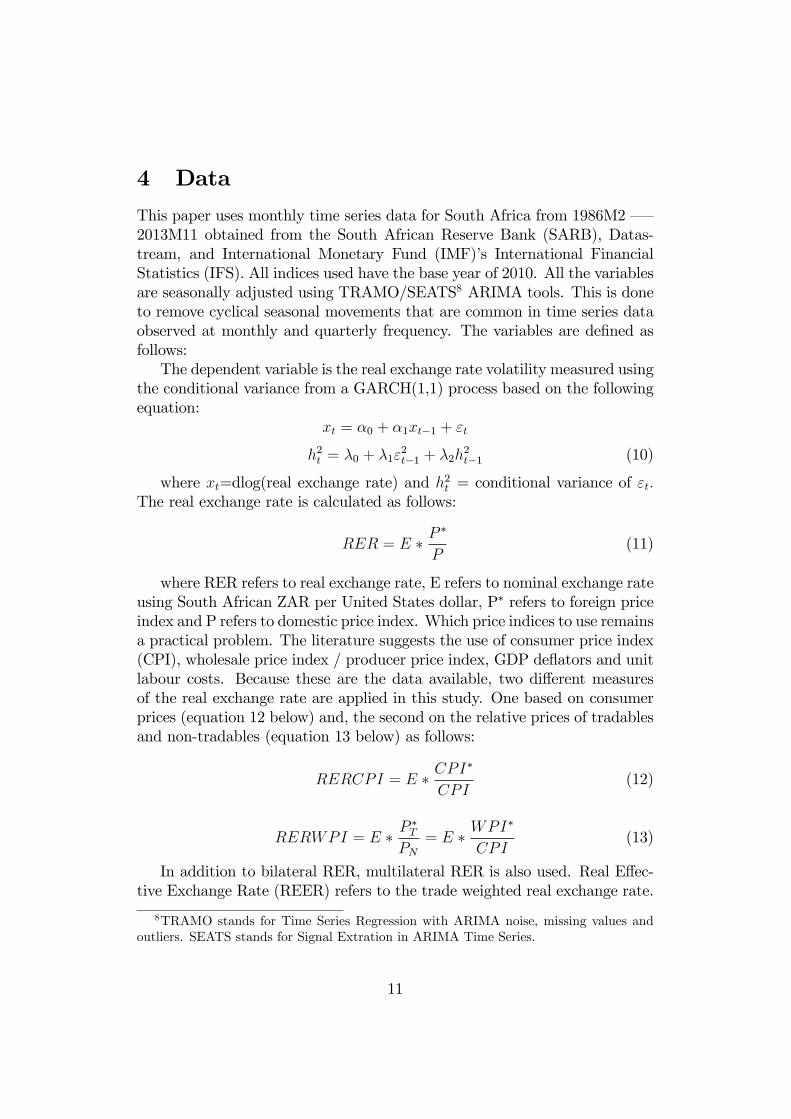
This paper uses monthly time series data for South Africa from 1986M2 � �2013M11 obtained from the South African Reserve Bank (SARB), Datas-tream, and International Monetary Fund (IMF)�s International FinancialStatistics (IFS). All indices used have the base year of 2010. All the variablesare seasonally adjusted using TRAMO/SEATS8 ARIMA tools. This is doneto remove cyclical seasonal movements that are common in time series dataobserved at monthly and quarterly frequency. The variables are de�ned asfollows:The dependent variable is the real exchange rate volatility measured using

the conditional variance from a GARCH(1,1) process based on the followingequation:

xt = �0 + �1xt�1 + "t

h2t = �0 + �1"2t�1 + �2h

2t�1 (10)

where xt=dlog(real exchange rate) and h2t = conditional variance of "t:The real exchange rate is calculated as follows:

RER = E � P�

P(11)

where RER refers to real exchange rate, E refers to nominal exchange rateusing South African ZAR per United States dollar, P� refers to foreign priceindex and P refers to domestic price index. Which price indices to use remainsa practical problem. The literature suggests the use of consumer price index(CPI), wholesale price index / producer price index, GDP de�ators and unitlabour costs. Because these are the data available, two di¤erent measuresof the real exchange rate are applied in this study. One based on consumerprices (equation 12 below) and, the second on the relative prices of tradablesand non-tradables (equation 13 below) as follows:

RERCPI = E � CPI�

CPI(12)

RERWPI = E � P�T

PN= E � WPI

�

CPI(13)

In addition to bilateral RER, multilateral RER is also used. Real E¤ec-tive Exchange Rate (REER) refers to the trade weighted real exchange rate.

8TRAMO stands for Time Series Regression with ARIMA noise, missing values andoutliers. SEATS stands for Signal Extration in ARIMA Time Series.

11

This data is for the 20 trading partners of South Africa, and based on manu-facturing goods. Both bilateral and multilateral nominal exchange rates areused. Nominal Exchange Rate (RUSNOM) refers to the nominal exchangerate for the ZAR per US dollar. Nominal E¤ective Exchange rate (NEER)refers to the trade weighted nominal exchange rate for the 20 trading partnersof South Africa.Independent variables include, �rstly Output volatility, where output is

measured using real GDP. This variable is used to proxy real productivityshocks. However, RGDP is not available in monthly frequency. As a result,monthly RGDP is interpolated using the cubic spline method from quarterlyRGDP. Secondly Money Supply volatility, which uses the narrow de�nitionof money supply, that is, M1. Openness is the third variable, in whichtrade openness (to) is measured as the ratio of exports of goods and servicesand imports of goods and services to nominal GDP. The values of the threevariables are all expressed in domestic currency. However, due to the non-existence of monthly GDP data, monthly GDP data is interpolated fromquarterly nominal series using the cubic spline method. The cubic splinemethod is common in the literature for converting either annual or quarterlyGDP data to monthly data (Chipili 2012)9.Foreign Reserves volatility is the fourth variable, and for this gross re-

serves are used. This variable is used for economic openness given thatthrough openness, central banks are able to accumulate foreign reserves.Commodity Prices volatility is the �fth variable and real gold price in do-mestic currency based on the pricing in London is used to proxy commodityprices. This study uses commodity price volatility as one of the determinantsof exchange rate volatility, unlike other studies that have used Terms of Trade(TOT) volatility. This follows the �nding by other researchers (Cashin, Ce-spedes & Sahay 2002, MacDonald & Ricci 2004, Frankel 2007) that TOTtends not to be signi�cant in most countries that are commodity exportersas one of the determinant of exchange rate, whilst commodity prices tend tobe signi�cant. MacDonald & Ricci (2004) assert two reasons for this. First,commodity prices are more accurate in terms of measurements, unlike TOT,which are based on arbitrary construction of country-speci�c export and im-port de�ators. Second, commodity prices data are frequently available foranalysis.Using real gold price volatility as an independent variable might cause

one to argue that there is reverse causality (i.e. endogeneity problem). For

9Chipili (2012) converts annual to monthly while Schneider et al.(2007), "Yemen: Ex-change Rate Policy in the Face of Dwindling Oil Exports" International Monetary FundWorking Paper No.0705, converts to quarterly.

12

example, Arezki et al. (2014) �nd that between 1979 and 1995 causalityruns from ZAR volatility to gold price volatility, but between 1995 and 2010,causality runs from gold price volatility to ZAR volatility. Accordingly, Irun Granger causality tests between ZAR volatility and gold price volatil-ity. The results for this test are shown in table 11 and indicate that for thestudy period for this paper, causality runs from gold price volatility to ZARvolatility only10. That is, gold price volatility causes ZAR volatility. Thereis therefore no issue of possible reverse causality. The sixth and last variableis Exchange Rate Regime, represented by a dummy variable. The dummyfor this variable takes the value of one from 1995M4 onwards and zero oth-erwise. Following the de�nition of the variables to be used in section 5 wheneconometric analysis is undertaken, �rst I present the preliminary tests forthe variables in the next section.

<Insert Table 11 Here>

4.1 Descriptive Statistics

Estimating empirical models using time series data requires the variablesbe stationary, implying unit root tests should be done before carrying outany analysis. Accordingly, I apply the Augmented Dickey-Fuller (ADF) andPhillips-Perron (PP) tests to �nd the order of integration of the variables.Table 3 shows that all the variables are integrated of order one {I(1)} whiletable 4 indicates that all the variables except trade openness are integratedof order one {I(1)}.

<Insert Table 3 and 4 Here>After �nding the stationarity properties of all the variables, I �nd the

summary statistics of all the stationary variables to show some key stylisedfacts. Table 5 indicates that the variables exhibit similarities to the behaviourof �nancial time series. That is, having excess kurtosis, and not following anormal distribution. For example, eight out of ten variables indicate excesskurtosis. The kurtosis of the standard normal distribution is three. Theskewness of the variables is not equal to zero, which implies the variables donot follow a standard normal distribution. Using the Jarque-Bera statistic,table 5 shows that nine out of ten variables are not normally distributed,given that they have signi�cant coe¢ cients. Furthermore, table 5 showsthat money supply and output varies less than the exchange rate (using thebilateral ZAR/US dollar and nominal e¤ective exchange rates) based on the

10The table reported in the appendix shows that one lag is used. However, I also tryusing lags from two up to 12 given that the data is monthly. The results con�rm thatcausality runs from gold price volatility to ZAR volatility only.

13

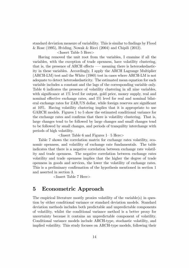
standard deviation measure of variability. This is similar to �ndings by Flood& Rose (1995), Hviding, Nowak & Ricci (2004) and Chipili (2012).

<Insert Table 5 Here>Having removed the unit root from the variables, I examine if all the

variables, with the exception of trade openness, have volatility clustering,that is, the presence of ARCH e¤ects � �meaning there is heteroskedastic-ity in these variables. Accordingly, I apply the ARCH Lagrange Multiplier(ARCH-LM) test and the White (1980) test in cases where ARCH-LM is notadequate to detect heteroskedasticity. The estimated mean equation for eachvariable includes a constant and the lags of the corresponding variable only.Table 6 indicates the presence of volatility clustering in all nine variables,with signi�cance at 1% level for output, gold price, money supply, real andnominal e¤ective exchange rates, and 5% level for real and nominal bilat-eral exchange rates for ZAR/US dollar, while foreign reserves are signi�cantat 10%. Having volatility clustering implies that it is appropriate to useGARCH models. Figures 1 to 5 show the estimated conditional variance forthe exchange rates and con�rms that there is volatility clustering. That is,large changes tend to be followed by large changes and small changes tendto be followed by small changes, and periods of tranquility interchange withperiods of high volatility.

<Insert Table 6 and Figures 1�5 Here>Table 7 shows the correlation matrix for exchange rates volatility, eco-

nomic openness, and volatility of exchange rate fundamentals. The tableindicates that there is a negative correlation between exchange rate volatil-ity and trade openness. The negative correlation between exchange ratesvolatility and trade openness implies that the higher the degree of tradeopenness in goods and services, the lower the volatility of exchange rates.This is a preliminary con�rmation of the hypothesis mentioned in section 1and asserted in section 3.

<Insert Table 7 Here>

5 Econometric Approach

The empirical literature mostly proxies volatility of the variable(s) in ques-tion by either conditional variance or standard deviation models. Standarddeviation methods includes both predictable and unpredictable componentsof volatility, whilst the conditional variance method is a better proxy foruncertainty because it contains an unpredictable component of volatility.Conditional variance models include ARCH-type, stochastic volatility, andimplied volatility. This study focuses on ARCH-type models, following their

14

introduction by Engle (1982) and their extension by Bollerslev (1986).The exchange rates exhibit volatility clustering whereby large changes

tend to be followed by large changes, and small changes by small changes.Periods of tranquility interchange with periods of high volatility, makingsuccessive exchange rate changes dependent on each other (Kwek & Koay2006, Chipili 2012). The empirical literature con�rms that exchange rates,like other �nancial time series, show non-linear behaviour (Chipili 2012).Such behaviour can be estimated using GARCH models, given that GARCHmodels are able to model and forecast time-varying variance.This study therefore utilises GARCH(1,1) and EGARCH(1,1) models to

examine the sources of exchange rate volatility in South Africa. A GARCH(1,1)model is adopted, following the literature, which shows that such a modelis parsimonious, even though higher order models do exist. The estimatedempirical equations are:Mean equation for exchange rate volatility

�xt = �0 +

qXi=1

�i�xt�1 + �1�Outputt + �2�MS1t + �3�Opent (14)

+�4�Fxrest + �5�Rgoldpt + �6ExrateRe gimet + "t

Variance equation for exchange rate volatility using a GARCH(1,1) method

h2t = �0 + �1"2t�1 + �h

2t�1 + 'ExrateRe gimet + �1�Outputt + (15)

�2�MS1t + �3�Opent + �4�Fxrest + �5�Rgoldpt + vt

Variance equation for exchange rate volatility using an EGARCH(1,1)method

ln(h2t ) = �0 + �1("t�1=h0:5t�1) + �1("t�1=h

0:5t�1) + � ln(h

2t�1) + (16)

'ExrateRe gimet + �1�Outputt + �2�MS1t +

�3�Opent + �4�Fxrest + �5�Rgoldpt + vt

where �xt is the logarithmic �rst di¤erence in the exchange rate; "t isresiduals that are used to test for the presence of ARCH e¤ects in the ex-change rate; q is the lag length; h2t is conditional variance of xt derived fromGARCH(1,1); �0; �i; �1;:::;6, �1; �0;1; �; ' and �1; :::; �5 are parameter coe¢ -cients to be estimated. Even though the objective of the study is to �ndmacroeconomic factors that drive exchange rate volatility, the explanatory

15

variables are also included in the mean equation. This is done because ex-change rate volatility is uncertain and as such the impact of exchange ratelevels should be controlled for. This is also because at monthly frequency,fundamentals matter for exchange rate movements. This di¤ers from thestudy by Fidrmuc & Horváth (2008), who do not include explanatory vari-ables in the mean equation (they only include lagged values of the exchangerate) because at daily frequency, fundamentals do not matter much in ex-plaining the movements of the exchange rate. An EGARCH model is alsoestimated because the literature shows that asset prices react di¤erentlyto bad and good news. This indicates that it is also appropriate to esti-mate GARCH models with asymmetry e¤ects. There are two models withasymmetry e¤ects namely, threshold GARCH (TGARCH) and exponentialGARCH (EGARCH) models. However, this study uses an EGARCH modelonly because, according to Enders (2010), this model has advantages over theTGARCH model. An advantage of the EGARCH model is that it does notrequire restriction of non-negativity of coe¢ cients, as in a GARCH model.

6 Results

In estimating the GARCH models, various AR(p) model speci�cations forthe mean equation are used together with the variance equation. That is,estimating equations 14 and 15 for a GARCH(1,1) model, and equations 14and 16 for an EGARCH model. The best model is chosen, based on thediagnostic tests of standardised residuals, which show the absence of ser-ial correlation and no remaining ARCH e¤ects. When both GARCH(1,1)and EGARCH(1,1) are signi�cant for a speci�c exchange rate series, thebest model is also based on the model with the larger value of log likeli-hood, and the smallest values for Akaike Information Criteria (AIC) andSchwartz Information Criteria (SIC). The exchange rate series estimated in-clude real e¤ective exchange rate (REER), nominal e¤ective exchange rate(NEER), real bilateral exchange rate for the ZAR/US dollar, measured us-ing consumer price indices for both countries (RERCPI), and one using thewholesale price index for the foreign country and consumer price index for thedomestic country (RERWPI), and nominal bilateral ZAR/US dollar (RUS-NOM). Accordingly, the Q-statistic for standardised residuals, the Q-statisticfor squared standardised residuals, and the ARCH-LM in table 10 indicatethat there is no serial autocorrelation and no ARCH e¤ects remaining, giventhe insigni�cant p-values. The results show that conditional volatility is per-sistent and mean reverting in all exchange rates, given that h2t�1 coe¢ cientis signi�cant and less than one, as shown in tables 8 and 9.

16

<Insert Tables 8, 9 and 10 Here>The results for the EGARCH models show that the asymmetric term is

insigni�cant for RERCPI, RERWPI, RUSNOM and NEER series, while itis signi�cant and negative for the REER series at 10% level. This suggeststhat there is no impact of news e¤ect on the RERCPI, RERWPI, RUSNOMand NEER series at monthly level. This is in line with the e¢ cient markethypothesis which states that the e¤ect of news on asset prices like exchangerates clears fast and is immediately re�ected in the changes of the asset pricein question. At monthly frequency therefore news might have less e¤ect.These results are similar to other studies that do not �nd signi�cant e¤ectsof asymmetric GARCH models at monthly frequency, like those of Jabeen& Khan (2014) and Chipili (2012). The signi�cance of EGARCH, usingREER suggests that negative news leads to a higher increase in exchangerate volatility, compared to positive news.In addition, the results about insigni�cance of the asymmetric term which

captures the impact of news, suggests that the behaviour of the exchangerate should also be analysed using short-term periods, for example, daily orintraday data. This follows some researchers (see e.g. Flood & Taylor 1996,MacDonald 1999, Morana 2009) who argue that exchange rate movementscannot always be explained by �ow demand and supply components, but byusing market microstructure models.Conditional volatility persists for about a month on average following a

shock in REER, NEER and RERCPI based on the half-life (HL) measure.But conditional volatility persists for about six months and 12 months onaverage following a shock in RUSNOM and RERWPI series respectively.The persistence of past shocks on conditional volatility measured by HL iscalculated as log(0.5) / log(h2t�1). HL then captures the period it takes for ashock to volatility to decrease to half its original size and h2t�1 is the speedof convergence to the steady state level. Furthermore, the results show thatREER and RUSNOM are GARCH(1,1) models, given the signi�cance of both"2t�1 and h

2t�1 terms: However, for RERCPI, RERWPI and NEER series, the

results indicate the presence of strong GARCH e¤ects, given the signi�canceof h2t�1 only, a result which is similar to the study by Singh (2002).Given the study�s objective of �nding the determinants of exchange rate

volatility, only the parameters in the variance equation(s) are analysed. Theresults show that the exchange rate regime dummy is positive and signi�-cant. This means that switching to a �oating exchange rate system leads tosigni�cantly more exchange rate volatility, which is consistent with most �nd-ings in the literature (see e.g. Canales-Kriljenko & Habermeier 2004, Stanc¬k2007, Chipili 2012) and the hypothesis of the ZAR behaviour as mentionedin section 1 by some researchers (see e.g. Arezki et al. 2014, Ricci 2005).

17

Using the exchange rate series of REER, NEER, RERWPI and RUSNOM,the results show that real gold price volatility has signi�cant and positive ef-fects on ZAR volatility. This implies that, as gold price volatility increases sodoes ZAR volatility. The signi�cance of real gold price volatility in in�uenc-ing ZAR volatility is similar to �ndings of the study by Arezki et al. (2014)who use a di¤erent method. The positive e¤ect is similar to studies that useterms of trade volatility (see e.g. Calderón 2004, Caporale et al. 2009, Jabeen& Khan 2014).The results indicate negative and signi�cant coe¢ cients for trade open-

ness using the RERWPI and RUSNOM series. This means that as tradeopenness increases, exchange rate volatility decreases. These results are inline with the theoretical model explained in section 3 and the results foundby other studies (Hau 2002, Calderón 2004, Caporale et al. 2009). However,using REER series, the results are positive and signi�cant, which is contraryto what theory indicates as mentioned in section 3. The positive and signif-icant value suggests that the degree of openness is low relative to what thetheory says. This implies that South Africa needs to increase its trading withthe 20 countries (or some of them) used in the construction of the REER bythe South African Reserve Bank. The results may also be a¤ected by the useof aggregate as opposed to bilateral trade data, as proposed by OCA theory(Hau 2002).Foreign reserves�volatility has a negative and signi�cant value for NEER.

This implies that changes in foreign reserves create con�dence in foreignmarkets, as argued by Hviding et al. (2004). This follows the argument thathigh and adequate international reserves are important for the preventionof a currency crisis, given that it signals the ability of the central bank tointervene in the foreign exchange market to stabilise the currency as well asboost con�dence for credit ratings.The results are negative and signi�cant for money supply volatility us-

ing the RERCPI series. This result is similar to Morana (2009) who �ndsa negative value in one country and Grydaki & Fountas (2010), who �ndnegative money supply volatility for Argentina and Chile. Carrera & Vuletin(2002) assert that the negative e¤ect is associated with increased interestrates, which lead to a decrease in money supply, and therefore a decline inexchange rate volatility. This suggests that the higher interest rates in SouthAfrica lead to more short-term capital in�ows, with the expectation of higherreturns, and thus increases exchange rate volatility.Output volatility has a positive and signi�cant e¤ect on RERWPI volatil-

ity. This is with the perspective of Friedman (1953) that exchange ratevolatility might be caused by macroeconomic instability. This means that,as instability increases, exchange rate volatility also increases. The coe¢ -

18

cients are insigni�cant when using RERCPI, RUSNOM and NEER seriesbut negative and signi�cant when using REER series. The negative value isalso similar to arguments presented by Friedman (1953) that it is possibleto have high output volatility leading to lower exchange rate volatility. Thismeans that there are some traders who are not concerned about instability ina country and want to invest regardless, as long as they will ultimately bene-�t. This phenomenon is widely seen in countries with many natural resources,for example, gold, or diamonds, or oil. Jabeen & Khan (2014) also �nd anegative and signi�cant relationship between output volatility and exchangerate volatility for Pakistan, using US dollar currency. The insigni�cant out-put value con�rms the claims of Flood & Rose (1995) that macroeconomicvolatility is not an important source of exchange rate volatility.

7 Conclusion

This paper investigates the determinants of real and nominal exchange ratevolatility using both bilateral (ZAR/US dollar) and e¤ective exchange ratesover the period 1986M2 � 2013M11 for South Africa. Using GARCH(1,1)and EGARCH(1,1) models, the study has two objectives: First, it teststhe hypothesis that economic openness decreases exchange rate volatility inSouth Africa. Second, it examines other macroeconomic factors that causeexchange rate volatility. The results show that switching to a �oating ex-change rate system leads to an increase in ZAR volatility, as hypothesised bysome researchers (see e.g. Arezki et al. 2014, Ricci 2005). This is informed byevidence of a positive and signi�cant e¤ect of a dummy variable post March1995 when South Africa liberalised its capital account. The results also showthat trade openness decreases ZAR volatility in South Africa using, the realand nominal bilateral ZAR/US dollar, and that other macroeconomic factorsalso in�uence ZAR volatility.The results for macroeconomic factors are summarised as follows: Real

gold price volatility increases ZAR volatility. The signi�cance of this variablein in�uencing exchange rate volatility is similar to �ndings in the study byArezki et al. (2014), who use a di¤erent method. Foreign reserves�changesreduce exchange rate volatility, which is in line with the �nding by Hvid-ing et al. (2004). Money supply volatility in�uences exchange rate volatilitynegatively, which suggest that increases in the interest rate leads to higherexchange rate volatility. The results also indicate that output volatility in-creases exchange rate volatility, using bilateral exchange rate. However, whenusing the real e¤ective exchange rate, the results between output volatilityand exchange rate volatility are the opposite. This is in line with the argu-

19

ments by Friedman (1953) and �ndings by Jabeen & Khan (2014).However, the results indicate that real factors (commodity prices volatil-

ity, output volatility, and openness) have higher magnitudes of in�uence,compared to monetary factors. An increase in exchange rate volatility mighthurt the economy via adverse e¤ects on employment growth and trade. Thissuggests that the South Africa government should focus more on real factorsif they aim to reduce exchange rate volatility. For example, it is necessaryto evaluate the costs of increasing openness and understand the relationshipbetween exchange rate volatility and fundamentals, rather than just focusingon exchange rate levels. This follows the recent debate on whether capitalcontrols are appropriate, in view of surges in capital in�ows into emergingmarkets. The fact that monetary factors also in�uence exchange rate volatil-ity implies that monetary authorities also have a part to play in reducingexchange rate volatility.

References

Amor, T. H. & Sarkar, A. U. (2008). Financial integration and real exchangerate volatility: Evidence from South and South East Asia, InternationalJournal of Business and Management 3(1): P112.

Arezki, R., Dumitrescu, E., Freytag, A. & Quintyn, M. (2014). Commodityprices and exchange rate volatility: Lessons from South Africa�s capitalaccount liberalization, Emerging Markets Review 19: 96�105.

Aron, J., Elbadawi, I. & Kahn, B. (1997). Real and monetary determinantsof the real exchange rate in South Africa, University of Oxford.

Aye, G. C., Gupta, R., Moyo, P. S. & Pillay, N. (2014). The impact ofexchange rate uncertainty on exports in South Africa, Journal of Inter-national Commerce, Economics and Policy .

Bayoumi, T. & Eichengreen, B. (1998). Exchange rate volatility and inter-vention: implications of the theory of optimum currency areas, Journalof International Economics 45(2): 191�209.

Bleaney, M. (2008). Openness and real exchange rate volatility: in search ofan explanation, Open Economies Review 19(2): 135�146.

Bollerslev, T. (1986). Generalized autoregressive conditional heteroskedas-ticity, Journal of econometrics 31(3): 307�327.

20

Calderón, C. (2004). Trade openness and real exchange rate volatility: paneldata evidence, Central Bank of Chile Working Paper 294 (294).

Canales-Kriljenko, J. I. & Habermeier, K. (2004). Structural factors a¤ectingexchange rate volatility: A cross-section study, International MonetaryFund Working Paper No.147 .

Caporale, G., Amor, T. & Rault, C. (2009). Sources of real exchange ratevolatility and international �nancial integration: A dynamic gmm paneldata approach, Brunel University West London, Working Paper Number09-21 .

Carrera, J. & Vuletin, G. (2002). The e¤ects of exchange rate regimes on realexchange rate volatility, A Dynamic Panel Data Approach. LACEA .

Cashin, P., Cespedes, L. & Sahay, R. (2002). Developing country real ex-change rates: Howmany are commodity countries?, IMFWorking Paper02/223 (Washington: Intemational Monetary Fund) .

Chipili, J. M. (2012). Modelling exchange rate volatility in Zambia, TheAfrican Finance Journal 14 (2): 85�107.

Devereux, M. B. & Lane, P. R. (2003). Understanding bilateral exchangerate volatility, Journal of International Economics 60(1): 109�132.

Dornbusch, R. (1976). Expectations and exchange rate dynamics, The Jour-nal of Political Economy pp. 1161�1176.

Enders, W. (2010). Applied Econometric Time Series, Third Edition, Vol. 9,John Wiley & Sons.

Engle, R. (1982). Autoregressive conditional heteroscedasticity with esti-mates of the variance of United Kingdom in�ation, Econometrica: Jour-nal of the Econometric Society pp. 987�1007.

Farrell, G. (2001). Capital controls and the volatility of South African ex-change rates, South African Reserve Bank Occasional Paper No.15 .

Faulkner, D. & Makrelov, K. (2008). Determinants of the equilibrium ex-change rate for South Africa�s manufacturing sector and implicationsfor competitiveness, Being a Draft of a Working Paper of the NationalTreasury of South Africa. Cited at http://www. treasury. gov. za .

21

Fidrmuc, J. & Horváth, R. (2008). Volatility of exchange rates in selected newEU members: Evidence from daily data, Economic Systems 32(1): 103�118.

Flood, R. P. & Rose, A. K. (1995). Fixing exchange rates a virtual quest forfundamentals, Journal of Monetary Economics 36(1): 3�37.

Flood, R. P. & Taylor, M. P. (1996). Exchange rate economics: what�s wrongwith the conventional macro approach?, The microstructure of foreignexchange markets, University of Chicago Press, pp. 261�302.

Frankel, J. (2007). On the rand: determinants of the South African exchangerate, South African Journal of Economics 75(3): 425�441.

Friedman, M. (1953). The case for �exible exchange rates, Essays in PositiveEconomics(pp. 157-203), Chicago: University of Chicago Press .

Grydaki, M. & Fountas, S. (2009). Exchange rate volatility and outputvolatility: A theoretical approach*, Review of International Economics17(3): 552�569.

Grydaki, M. & Fountas, S. (2010). What explains nominal exchange ratevolatility? Evidence from the Latin American countries, Department ofEconomics, University of Macedonia, Discussion Paper No.10 .

Hau, H. (2002). Real exchange rate volatility and economic openness: theoryand evidence, Journal of money, Credit and Banking pp. 611�630.

Hviding, K., Nowak, M. & Ricci, L. A. (2004). Can higher reserves helpreduce exchange rate volatility?, International Monetary Fund WorkingPaper No.189 .

Jabeen, M. & Khan, S. A. (2014). Modelling exchange rate volatility bymacroeconomic fundamentals in pakistan, International EconometricReview (IER) 6(2): 59�77.

Kwek, K. T. & Koay, K. N. (2006). Exchange rate volatility and volatilityasymmetries: an application to �nding a natural dollar currency, AppliedEconomics 38(3): 307�323.

MacDonald, R. (1999). Exchange rate behaviour: are fundamentals impor-tant?, The Economic Journal 109(459): 673�691.

22

MacDonald, R. & Ricci, L. (2004). Estimation of the equilibrium real ex-change rate for SOUTH AFRICA, South African Journal of Economics72(2): 282�304.

Meese, R. & Rogo¤, K. (1983). Empirical exchange rate models of the sev-enties: Do they �t out of sample?, Journal of international economics14(1): 3�24.

Morana, C. (2009). On the macroeconomic causes of exchange rate volatility,International Journal of Forecasting 25(2): 328�350.

Mpofu, T. R. (2013). Real exchange rate volatility and employment growthin South Africa: The case of manufacturing.

Obstfeld, M. & Rogo¤, K. (1996). Foundations of international macroeco-nomics, 1996, MIT Press, Cambridge, MA.

Ricci, L. A. (2005). South Africa�s real exchange rate performance, PostApartheid South Africa: The First Ten Years pp. 142�155.

Rogo¤, K. (1999). Perspectives on exchange rate volatility, in: Feldstein, M.,ed., International Capital Flows, Chicago: University of Chicago Press,pp. 441-453 .

Saayman, A. (2007). The real equilibrium South African rand/US dollarexchange rate: A comparison of alternative measures, International Ad-vances in Economic Research 13(2): 183�199.

Singh, T. (2002). On the garch estimates of exchange rate volatility in India,Applied Economics Letters 9(6): 391�395.

Stanc¬k, J. (2006). Determinants of exchange rate volatility: The case ofthe new EU members, Center for Economic Research and GraduateEducation-Economics Institute, Discussion Paper No.158 .

Stanc¬k, J. (2007). Determinants of exchange rate volatility: The case of thenew EU members, The Czech Journal of Economics and Finance, 57(9-10): 414�432.

Todani, K. & Munyama, T. (2005). Exchange rate volatility and ex-ports in South Africa, South African Reserve Bank, presented at theTIPS/DPRU Forum, Pretoria, South Africa .

23

White, H. (1980). A heteroskedasticity-consistent covariance matrix estima-tor and a direct test for heteroskedasticity, Econometrica: Journal ofthe Econometric Society pp. 817�838.

8 Appendix

Table 1: Selected Developed and Emerging Market Currency Distributionof global exchange market (percentage shares of average daily turnover inApril)-1998 to 2013Currency 1998 2001 2004 2007 2010 2013United States dollar 86.8(1) 89.9(1) 88.0(1) 85.6(1) 84.9(1) 87.0(1)European euro ...(32) 37.9(2) 37.4(2) 37.0(2) 39.1(2) 33.4(2)Japanese yen 21.7(2) 23.5(3) 20.8(3) 17.2(3) 19.0(3) 23.0(3)British pound 11.0(3) 13.0(4) 16.5(4) 14.9(4) 12.9(4) 11.8(4)Australian dollar 3.0(6) 4.3(7) 6.0(6) 6.6(6) 7.6(5) 8.6(5)Canadian dollar 3.5(5) 4.5(6) 4.2(7) 4.3(7) 5.3(7) 4.6(7)Mexican peso 0.5(9) 0.8(14) 1.1(12) 1.3(12) 1.3(14) 2.5(8)Chinese renminbi 0.0(30) 0.0(35) 0.1(29) 0.5(20) 0.9(17) 2.2(9)Russian rouble 0.3(12) 0.3(19) 0.6(17) 0.7(18) 0.9(16) 1.6(12)Turkish lira ...(33) 0.0(30) 0.1(28) 0.2(26) 0.7(19) 1.3(16)Korean won 0.2(18) 0.8(15) 1.1(11) 1.2(14) 1.5(11) 1.2(17)South African rand 0.4(10) 0.9(13) 0.7(16) 0.9(15) 0.7(20) 1.1(18)Brazilian real 0.2(16) 0.5(17) 0.3(21) 0.4(21) 0.7(21) 1.1(19)Indian rupee 0.1(22) 0.2(21) 0.3(20) 0.7(19) 1.0(15) 1.0(20)Polish zloty 0.1(26) 0.5(18) 0.4(19) 0.8(17) 0.8(18) 0.7(22)Malaysian ringgit 0.0(27) 0.1(26) 0.1(30) 0.1(28) 0.3(25) 0.4(25)Chilean peso 0.1(24) 0.2(23) 0.1(25) 0.1(30) 0.2(29) 0.3(28)Note:the number outside the brackets represents the share of the currency while the

number in brackets represents the rank of the currency.

Source: Bank for International Settlements, Triennial Central Bank Survey (2013).

24

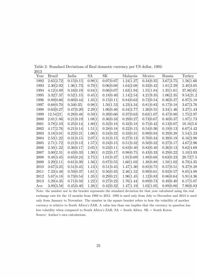
Table 2: Standard Deviations of Real domestic currency per US dollar, 1992-2013Year Brazil India SA SK Malaysia Mexico Russia Turkey1992 2.65[2.72] 0.15[0.15] 0.98[1] 0.07[0.07] 1.24[1.27] 0.34[0.35] 3.67[3.75] 1.56[1.60]1993 2.30[2.92] 1.36[1.73] 0.79[1] 0.06[0.08] 1.64[2.08] 0.33[0.42] 1.81[2.29] 2.40[3.05]1994 4.12[4.89] 0.16[0.19] 0.84[1] 0.06[0.07] 1.63[1.94] 1.55[1.84] 1.35[1.61] 37.86[45]1995 3.32[7.37] 0.52[1.15] 0.45[1] 0.18[0.40] 1.14[2.54] 4.21[9.35] 1.06[2.35] 9.54[21.2]1996 0.89[0.66] 0.60[0.44] 1.35[1] 0.15[0.11] 0.84[0.63] 0.72[0.54] 0.36[0.27] 6.97[5.18]1997 0.68[0.70] 0.340.35] 0.98[1] 1.50[1.53] 4.23[4.34] 0.81[0.83] 0.17[0.18] 3.67[3.76]1998 0.63[0.27] 0.47[0.20] 2.29[1] 1.06[0.46] 6.34[2.77] 1.26[0.55] 3.34[1.46] 3.27[1.43]1999 12.54[21] 0.28[0.48] 0.59[1] 0.39[0.66] 0.37[0.63] 0.63[1.07] 0.47[0.80] 1.75[2.97]2000 2.01[1.86] 0.21[0.19] 1.08[1] 0.36[0.33] 0.29[0.27] 0.73[0.67] 0.40[0.37] 1.87[1.73]2001 3.78[2.10] 0.25[0.14] 1.80[1] 0.32[0.18] 0.32[0.18] 0.75[0.42] 0.13[0.07] 10.16[5.63]2002 4.17[2.76] 0.21[0.14] 1.51[1] 0.28[0.18] 0.22[0.15] 0.54[0.36] 0.19[0.13] 6.67[4.42]2003 3.18[3.01] 0.22[0.21] 1.06[1] 0.34[0.32] 0.33[0.31] 0.99[0.94] 0.29[0.28] 5.54[5.23]2004 2.53[1.22] 0.31[0.15] 2.07[1] 0.31[0.15] 0.27[0.13] 0.70[0.34] 0.39[0.19] 6.16[2.98]2005 2.71[1.72] 0.21[0.13] 1.57[1] 0.24[0.15] 0.51[0.32] 0.50[0.32] 0.27[0.17] 4.67[2.96]2006 2.50[1.22] 0.36[0.17] 2.05[1] 0.23[0.11] 0.83[0.40] 0.83[0.40] 0.26[0.13] 9.62[4.69]2007 3.00[2.31] 0.43[0.33] 1.30[1] 0.22[0.17] 0.98[0.75] 0.43[0.33] 0.29[0.22] 5.10[3.93]2008 9.48[3.45] 0.65[0.24] 2.75[1] 1.01[0.37] 1.91[0.69] 1.88[0.68] 0.63[0.23] 20.72[7.54]2009 3.29[2.11] 0.61[0.39] 1.56[1] 0.87[0.55] 1.60[1.03] 1.38[0.88] 1.58[1.02] 6.79[4.35]2010 3.67[3.25] 0.51[0.45] 1.13[1] 0.51[0.45] 1.47[1.30] 0.85[0.75] 0.57[0.51] 9.37[8.28]2011 7.23[4.48] 0.59[0.37] 1.61[1] 0.56[0.35] 2.46[1.52] 0.99[0.61] 0.92[0.57] 8.05[4.98]2012 5.67[4.18] 0.73[0.54] 1.35[1] 0.29[0.21] 1.96[1.45] 1.12[0.83] 0.86[0.64] 5.91[4.36]2013 5.29[4.35] 0.71[0.58] 1.22[1] 0.27[0.22] 1.76[1.44] 0.89[0.73] 0.49[0.40] 6.17[5.07]Ave 3.89[3.58] 0.45[0.40] 1.38[1] 0.42[0.32] 1.47[1.19] 1.02[1.05] 0.89[0.80] 7.90[6.83]Note: the number not in the bracket represents the standard deviation for that year calculated using the real

exchange rate for the 12 months from 1993 to 2012. 1992 is used only from July to December and 2013 is used

only from January to November. The number in the square bracket refers to how the volatility of another

currency is relative to South Africa�s ZAR. A value less than one implies that the currency in question has

less volatility when compared to South Africa�s ZAR. SA = South Africa. SK = South Korea.

Source: Author�s own calculations.

25

Table 3: Unit Root Tests using Augmented Dickey-Fuller methodVariable ADF-statistic ADF-statistic Critical Values

levels �rst di¤erence 1% 5% 10% ProbLRERCPI -2.429 -13.356 -2.572 -1.942 -1.616 0.0000***LRERWPI -2.564 -12.680 -2.572 -1.942 -1.616 0.0000***LRUSNOM -2.172 -12.950 -2.572 -1.942 -1.616 0.0000***LREER -3.329 -13.404 -2.572 -1.942 -1.616 0.0000***LNEER -2.942 -13.295 -2.572 -1.942 -1.616 0.0000***LFXRES -3.224 -5.414 -2.572 -1.942 -1.616 0.0000***LM1 -1.450 -6.524 -2.572 -1.942 -1.616 0.0000***LOUTPUT -1.546 -2.911 -2.572 -1.942 -1.616 0.0036***LTO -3.053 -24.371 -2.572 -1.942 -1.616 0.0000***LRGOLDP -1.648 -15.421 -2.572 -1.942 -1.616 0.0000***

Notes: Variables are de�ned as in section 4. *** indicates signi�cant at 1%. The values in levels

include the constant and trend.

Source: Output using Eviews 8.

26

Table 4: Unit Root Tests using Phillips-Perron methodVariable PP-statistic PP-statistic Critical Values

levels �rst di¤erence 1% 5% 10% ProbLRERCPI -2.189 -13.172 -2.572 -1.942 -1.616 0.0000***LRERWPI -3.064 -13.785 -2.572 -1.942 -1.616 0.0000***LRUSNOM -1.746 -12.898 -2.572 -1.942 -1.616 0.0000***LREER -3.000 -12.999 -2.572 -1.942 -1.616 0.0000***LNEER -2.340 -13.185 -2.572 -1.942 -1.616 0.0000***LFXRES -2.623 -18.391 -2.572 -1.942 -1.616 0.0000***LM1 -1.070 -20.653 -2.572 -1.942 -1.616 0.0000***LOUTPUT -1.678 -6.152 -2.572 -1.942 -1.616 0.0000***LTO -7.624 -3.986 -3.423 -3.135 0.0000***LRGOLDP -1.816 -15.443 -2.572 -1.942 -1.616 0.0000***

Notes: Variables are de�ned as in section 4. *** indicates signi�cant at 1%. The values in levels

include a constant and trend.

Source: Output using Eviews 8.

Table 5: Descriptive Statistics: 1986M2 � 2013M11Variables Obs Mean Std.Dev Skewness Kurtosis Jarque-BeraDRERCPI 334 -5.24E-05 0.0339 0.6254 8.4403 433.6542***DRERWPI 334 -0.000262 0.0343 0.2981 6.6296 188.2813***DRUSNOM 334 0.004391 0.0348 0.7678 8.2241 412.6215***DREER 334 -0.000243 0.0263 -1.8816 15.266 2291.028***DNEER 334 -0.005165 0.0300 -1.1637 10.6334 8886.2750***DFXRES 334 0.018038 0.0707 2.3148 21.7178 5174.093***DM1 334 0.011719 0.0278 0.5286 4.3713 41.7200***DOUTPUT 334 0.002266 0.0091 -0.4648 2.4613 16.06644***DTO 334 -0.000512 0.0886 -0.1780 2.9423 1.8094DRGOLDP 334 0.006050 0.0428 0.7261 5.9301 148.8278***

Notes: *** indicates signi�cant at 1%. Obs = number of observation. Std.Dev = standard deviation

Source: Output using Eviews 8.

27

Table 6: Heteroskedasticity testVariable F-statistic Prob. F Obs*R-squared ProbDRERCPI 4.0457 0.0185** 7.9696 0.0186**(w)DRERWPI 4.3226 0.0140** 8.5010 0.0143**(w)DRUSNOM 4.3829 0.0132** 8.6167 0.0135**(w)DREER 14.1441 0.0002*** 13.6450 0.0002***(lm)DNEER 6.3059 0.0021*** 12.2579 0.0022***(w)DFXRES 2.3356 0.0554* 9.2209 0.0558*(lm)DM1 9.4531 0.0023*** 9.2455 0.0024***(lm)DOUTPUT 27.2892 0.0000*** 25.3576 0.0000***(lm)DRGOLDP 3.6182 0.0279** 7.1450 0.0281***(lm)

Notes:***,**,* indicates signi�cant at 1%,5% and 10% respectively. (w) indicates that the

white test is used and (lm) indicates that the ARCH-LM test is used.

Source: Output using Eviews 8.

28

Table7:Correlationmatrixforallthevariables

rercpi

rerwpi

rusnom

reer

neer

fxres

m1

output

rgoldp

Dto

rercpi

1.000

rerwpi

0.913

1.000

rusnom

0.980

0.920

1.000

reer

0.873

0.764

0.866

1.000

neer

0.928

0.865

0.909

0.938

1.000

fxres

-0.015

-0.071

-0.042

0.018

0.013

1.000

m1

0.073

0.170

0.054

0.076

0.052

0.021

1.000

output

0.028

-0.042

0.012

0.040

0.024

-0.006

-0.241

1.000

rgoldp

0.664

0.630

0.694

0.649

0.655

-0.056

-0.071

0.088

1.000

Dto

-0.072

-0.064

-0.070

-0.008

-0.023

-0.010

-0.032

-0.018

-0.024

1.000

Notes:allthevariablesexcepttradeopenness(Dto)arede�nedasvolatility.

Source:OutputusingEviews8.

29

Figure 1: Estimated Conditional Variance for RERCPI0

.002

.004

.006

.008

RERC

PI V

OLA

TIL

ITY

1985m1 1990m1 1995m1 2000m1 2005m1 2010m1 2015m1time

Source: Output using Stata 13.1

Figure 2: Estimated Conditional Variance for RERWPI

0.0

02.0

04.0

06RE

RWPI

 VO

LATI

LIT

Y

1985m1 1990m1 1995m1 2000m1 2005m1 2010m1 2015m1time

Source: Output using Stata 13.1

30

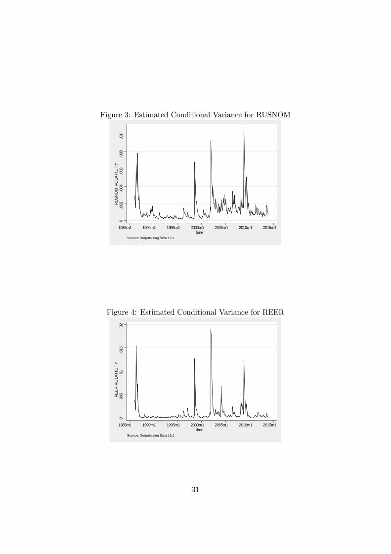
Figure 3: Estimated Conditional Variance for RUSNOM0

.002

.004

.006

.008

.01

RUSN

OM

 VO

LATI

LITY

1985m1 1990m1 1995m1 2000m1 2005m1 2010m1 2015m1time

Source: Output using Stata 13.1

Figure 4: Estimated Conditional Variance for REER

0.0

05.0

1.0

15.0

2RE

ER V

OLA

TILI

TY

1985m1 1990m1 1995m1 2000m1 2005m1 2010m1 2015m1time

Source: Output using Stata 13.1

31

Figure 5: Estimated Conditional Variance for NEER

0.0

05.0

1.0

15NE

ER V

OLA

TILI

TY

1985m1 1990m1 1995m1 2000m1 2005m1 2010m1 2015m1time

Source: Output using Stata 13.1

32

Table8:GARCH(1,1)results

Parameters

RERCPI

RERWPI

RUSNOM

REER

NEER

Meaneq.

constant

-0.0031

-0.0031*

0.0034**

0.0002

-0.0056***

OUTPUT

-0.0221

0.2601**

0.1507

-0.1238

0.0972

MS1

-0.0243

0.0268

0.0393

0.00644

0.0098

TO

-0.0143

0.0057

0.0050

-0.0058

0.0093

FXRES

0.0352

0.0229

0.0296**

-0.0352***

-0.0274**

RGOLDP

0.4236***

0.4102***

0.3828***

-0.2848***

-0.3683***

DUM95

0.0011

0.0012

-0.0026

0.0018

0.0056***

AR(1)

0.2969***

0.2763***

0.3260***

0.4518***

0.2369***

AR(2)

-0.1018**

-0.1402***

-0.0874**

-0.1456**

-0.1144***

AR(3)

-0.0546

0.0584

AR(4)

0.0120

Varianceeq.

constant

0.000425***

1.82E-05***

5.69E-06***

9.35E-05***

0.000138***

"2 t�1

0.051049

-0.008295

0.042193*

0.151845**

-0.034893

h2 t�1

0.456813***

0.945597***

0.897797***

0.418091***

0.629204***

OUTPUT

0.003226

0.003028**

0.002112

-0.005413***

-0.001911

MS1

-0.005038***

-0.000583

0.000151

-0.000181

-0.001079

TO

0.000839

-0.001149***

-0.001027***

0.000388*

-9.12E-05

FXRES

-0.000196

-2.57E-05

7.87E-05

4.62E-05

-0.000392***

RGOLDP

0.002519

0.001221**

0.001453*

0.001101***

0.002243***

DUM95

-5.58E-05

1.64E-05***

1.95E-05**

4.58E-05**

7.57E-05

"2 t�1+h2 t�1

0.5078

0.9373

0.9401

0.5699

0.5943

Notes:***,**,*indicatessigni�cantat1%,5%and10%respectively.eqstandsforequation.Thevariablesare

de�nedinsection4.Thep-valuesarebasedonBollerslev-Wooldridgerobuststandarderrorsandcovariance.

Source:OutputusingEviews8.

33

Table9:EGARCH(1,1)results

Parameters

RERCPI

RERWPI

RUSNOM

REER

NEER

Meaneq.

constant

-0.0012

-0.0036**

0.0028*

5.41E-05

-0.0048***

OUTPUT

0.0990

0.2899**

0.2521**

-0.1589**

0.1201*

MS1

-0.0059

0.0565

0.0308

-0.0012

-0.0175

TO

-0.0076

0.0081

-0.0041

0.0048

0.0238***

FXRES

0.0275*

0.0321***

0.0240*

-0.0174***

-0.0134*

RGOLDP

0.3721***

0.390450***

0.3702***

-0.2194***

-0.3588***

DUM95

-0.0015

0.000129

-0.0029

0.0023

0.0058***

AR(1)

0.3293***

0.311881***

0.3664***

0.4983***

0.3068***

AR(2)

-0.1092**

-0.155444***

-0.1072**

-0.1506***

-0.1592***

AR(3)

0.110265***

-0.0502

AR(4)

-0.106173**

0.1089***

AR(5)

-0.006562

-0.1083***

AR(6)

-0.085971**

0.0542*

Varianceeq.

constant

-0.327496***

-0.241081***

-0.163864***

-2.052698**

-0.898405***

�1{"t�1=(ht�1)0:5}-0.153281**

-0.082110

-0.086716

0.151501

-0.349279***

�1{"t�1=(ht�1)0:5}

0.015563

0.049909

0.041082

-0.127942*

-0.008927

ln(ht�1)

0.945410***

0.966386***

0.978000***

0.792796***

0.866341***

OUTPUT

10.02419**

4.311940

7.945157**

-17.36371***

1.786508

MS1

-1.453856

0.135521

1.161004

1.6748

1.814034

TO

-0.448686

-0.979166

-0.390136

0.1495

-0.632399*

FXRES

0.490851

-0.187143

0.087639

-0.387790

-1.355489***

RGOLDP

1.693462**

-0.078400

0.666949

7.983027***

5.110445***

DUM95

0.018627

0.059399***

0.040779***

0.191110

0.108753***

Notes:***,**,*indicatessigni�cantat1%,5%and10%respectively.eqstandsforequation.Thevariablesare

de�nedinsection4.

Source:OutputusingEviews8.

34

Table10:Diagnostictests

GARCH(1,1)

RERCPI

RERWPI

RUSNOM

REER

NEER

Q-test:v t

Q(2)

2.0625(0.357)

2.0334(0.362)

1.2700(0.530)

0.3042(0.859)

1.3215(0.516)

Q(4)

4.4159(0.353)

6.0916(0.192)

1.7851(0.775)

2.3602(0.670)

1.4559(0.834)

Q(6)

4.4917(0.610)

7.0069(0.320)

1.8693(0.931)

5.9833(0.425)

5.9960(0.424)

Q-test:v2 t

Q(2)

0.5023(0.778)

1.2471(0.536)

0.0247(0.988)

3.5327(0.171)

0.6145(0.735)

Q(4)

5.1905(0.268)

1.5755(0.813)

0.5093(0.973)

3.6964(0.449)

0.6742(0.954)

Q(6)

6.3759(0.382)

5.5920(0.470)

4.2332(0.645)

4.6683(0.587)

3.7986(0.704)

ARCH-LM

0.2295(0.6317)

0.0003(0.9861)

0.0004(0.9832)

2.5127(0.1129)

0.0068(0.9343)

Loglikelihood

754.1531

774.8246

774.8326

920.2729

822.4597

AIC

-4.4347

-4.5592

-4.5592

-5.4458

-4.8634

SIC

-4.2284

-4.3529

-4.3529

-5.2275

-4.6331

EGARCH(1,1)

Q-test:v t

Q(2)

0.9681(0.616)

1.0351(0.596)

0.8492(0.654)

0.3002(0.861)

1.9718(0.373)

Q(4)

3.2902(0.510)

1.3807(0.848)

2.8105(0.590)

0.9172(0.922)

4.8371(0.304)

Q(6)

3.7941(0.705)

7.6779(0.263)

3.1076(0.795)

3.3576(0.763)

7.3571(0.289)

Q-test:v2 t

Q(2)

2.0938(0.351)

1.0351(0.596)

0.0900(0.956)

3.9200(0.141)

1.9697(0.373)

Q(4)

5.0341(0.284)

1.3807(0.848)

0.8412(0.933)

5.9449(0.203)

2.7384(0.603)

Q(6)

9.4561(0.150)

7.6779(0.263)

4.6388(0.591)

8.9929(0.174)

6.3968(0.380)

ARCH-LM

0.2136(0.6440)

0.1870(0.6654)

0.0006(0.9798)

2.0755(0.1497)

1.2537(0.2628)

Loglikehood

777.5297

777.5982

786.9701

944.3293

847.5239

AIC

-4.5695

-4.6012

-4.6263

-5.6179

-4.9911

SIC

-4.3517

-4.3352

-4.4086

-5.3519

-4.7733

Notes:Q-test:v tandQ-test:v2 taretestsforthepresenceofserialcorrelationandremainingARCH/GARCHe¤ectsconductedon

Ljung-BoxQ-statisticofstandardisedandsquaredstandardisedresidualsrespectively.Thenumberinbracketsisthep-value.The

optimallaglength(k)of6fortheQ-teststatisticischosenaccordingtothesuggestionbyTsay(2002)thatk=ln(T)whereTisthe

numberofobservations.AICisAkaikeinfocriterionandSICisSchwarzcriterion.

Source:OutputusingEviews8.

35

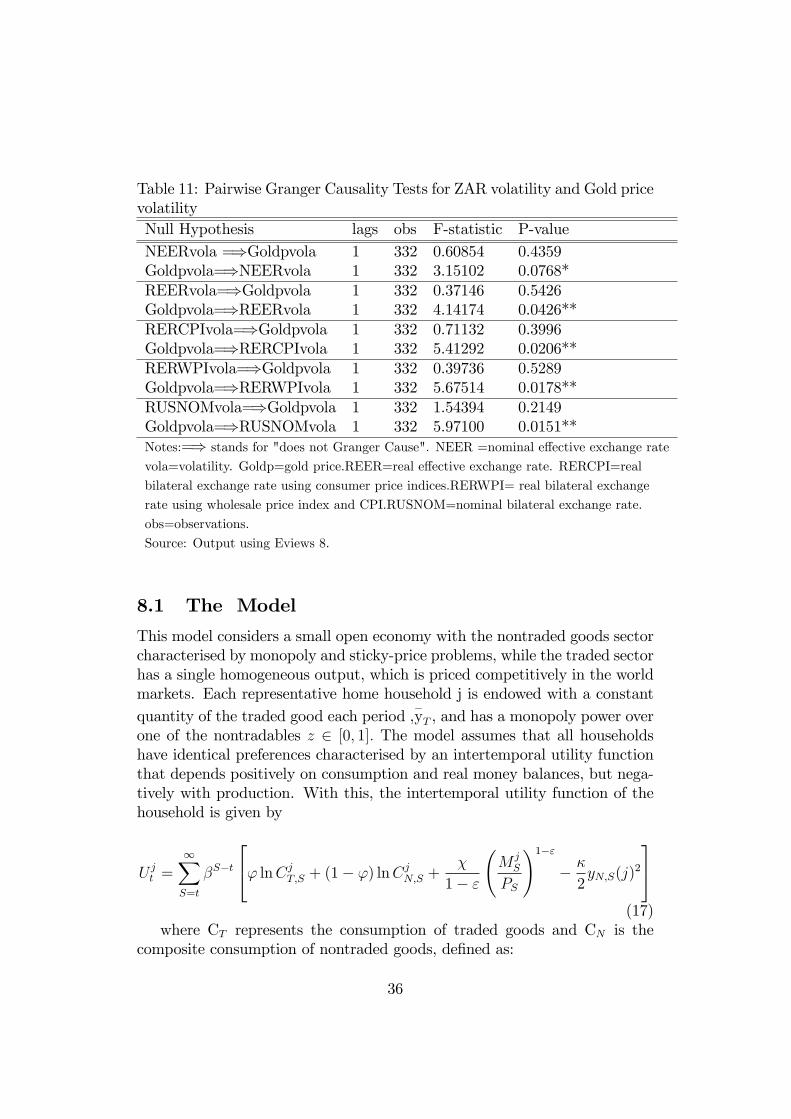
Table 11: Pairwise Granger Causality Tests for ZAR volatility and Gold pricevolatilityNull Hypothesis lags obs F-statistic P-valueNEERvola =)Goldpvola 1 332 0.60854 0.4359Goldpvola=)NEERvola 1 332 3.15102 0.0768*REERvola=)Goldpvola 1 332 0.37146 0.5426Goldpvola=)REERvola 1 332 4.14174 0.0426**RERCPIvola=)Goldpvola 1 332 0.71132 0.3996Goldpvola=)RERCPIvola 1 332 5.41292 0.0206**RERWPIvola=)Goldpvola 1 332 0.39736 0.5289Goldpvola=)RERWPIvola 1 332 5.67514 0.0178**RUSNOMvola=)Goldpvola 1 332 1.54394 0.2149Goldpvola=)RUSNOMvola 1 332 5.97100 0.0151**Notes:=) stands for "does not Granger Cause". NEER =nominal e¤ective exchange rate

vola=volatility. Goldp=gold price.REER=real e¤ective exchange rate. RERCPI=real

bilateral exchange rate using consumer price indices.RERWPI= real bilateral exchange

rate using wholesale price index and CPI.RUSNOM=nominal bilateral exchange rate.

obs=observations.

Source: Output using Eviews 8.

8.1 The Model

This model considers a small open economy with the nontraded goods sectorcharacterised by monopoly and sticky-price problems, while the traded sectorhas a single homogeneous output, which is priced competitively in the worldmarkets. Each representative home household j is endowed with a constantquantity of the traded good each period ,

�yT , and has a monopoly power over

one of the nontradables z 2 [0; 1]: The model assumes that all householdshave identical preferences characterised by an intertemporal utility functionthat depends positively on consumption and real money balances, but nega-tively with production. With this, the intertemporal utility function of thehousehold is given by

U jt =

1XS=t

�S�t

24' lnCjT;S + (1� ') lnCjN;S + �

1� "

M jS

PS

!1�"� �2yN;S(j)

2

35(17)

where CT represents the consumption of traded goods and CN is thecomposite consumption of nontraded goods, de�ned as:

36

CN =

�Z 1

0

cN (z)��1� dz

� ���1

(18)

Consumption based price index, P, is de�ned as the minimum cost ofbuying an additional unit of real consumption C'TC

1�'N : This price index is

represented as:

P =P'T P

1�'N

''(1� ')1�' (19)

where PT represents the price of tradables and PN is the nontraded goodsprice index, de�ned as

PN =

�Z 1

0

pN(z)1��dz

� 11��

(20)

where pN(z) is the price of nontraded good z: Domestic prices PT arelinked to a constant world prices P �T via the exchange rate, E. This is repre-sented as follows:

PT = EP�T (21)

In addition, the model assumes the existence of an international bondmarket with real bonds denominated in terms of tradables. The constantworld net interest rate in tradables is denoted by r and �(1 + r) = 1: Theintertemporal budget constraint for the representative household j is denotedby

PT;tBjt+1 +M

jt = PT;t(1 + r)B

jt +M

jt�1 + pN;t(j)yN;t(j) + PT;t

�yT �(22)

PN;tCjN;t � PT;tC

jT;t � PT;t� t

where � t denotes taxes per capita in terms of the tradable goods while Btrepresents the bond portfolio. Abstracting from government spending, themodel assumes that the government balances its budget in units of tradablesand its constraint is as follows:

� t +Mt �Mt�1

PT;t= 0 (23)

Finally the preferences take the Constant Elasticity of Substitution (CES)form. This results in producers of non-traded goods facing the followingdemand curve:

ydN(j) =

�pN(j)

PN

���CAN (24)

37

where CAN represents the aggregate consumption of nontraded goods.Solving the household�s optimisation problem requires maximising equa-

tion 17 subject to equations 22 and 24 with respect to the choice variablesBjt+1;Mt; CN;t and yN;t: This results in the following four �rst-order condi-tions(FOC):

CjT;t+1 = CjT;t (25)

'

CjT;t= �

PT;tPt

�Mt

Pt

��"+ �

PT;tPT;t+1

'

CjT;t+1

!(26)

CjN;t =1� ''

�PT;tPN;t

�CjT;t (27)

y�+1�

N;t =

�(� � 1) (1� ')

��

� �CAN;t

� 1�1

CjN;t(28)

Equation 25 shows the Euler condition for optimal intertemporal con-sumption smoothing for traded goods. Equation 26 shows the utility max-imising trade-o¤ between consumption spending in period t and a combina-tion of one-period money holding and consumption spending in period t+1.Equation 27 states that the marginal utility of traded and nontraded con-sumption must be equal at any given time. Equation 28 depicts the conditionfor optimal monopolistic price setting. Hau (2002) states that equation 28is used to show the marginal consumption utility of an additional unit ofnontraded good as well as the marginal disutility of production of an addi-tional unit. As a result, a mark up of �=� � 1 is added by monopolisticallycompetitive �rms.Substituting equation 25 into equation 26 leads to the following expression

for the demand for real balances:

Mt

Pt= f

�'CT;t

PT;tPt�

1� � PT;tPT;t+1

�g 1" (29)

implying the demand for real balances depends on consumption of trad-ables, CT;t, changes in the price of tradables, PT;t / PT;t+1 and changes in thereal price of tradables, PT;t / Pt:Including government spending, the model assumes that government spend-

ing, G; is dissipative and does not a¤ect productivity or private utility. Italso assumes that government�s real consumption index takes the same gen-eral form as the private sector�s. With government spending, equation 23becomes:

Gt = � t +Mt �Mt�1

Pt(30)

38

Given that preferences take the CES form, the producers of non-tradedgoods take the form:

ydN;t =

�pN;t(j)

PN;t

��� �CAN +G

AN

�(31)

where CAN is home country�s private demand for non-traded goods andGAN

is home country�s public demand for non-traded goods. Implying solving theoptimisation problem including the government spending leads to equation28 only, changing to

y�+1�

N;t =

�(� � 1) (1� ')

��

� �CAN;t +G

AN;t

� 1�1

CjN;t(32)

39