detection of carbon monoxide (co) as a furnace...
TRANSCRIPT

Equation Chapter 1 Section 1 SANDIA REPORT SAND2007-0667 Unlimited Release Printed February 2007
Detection of Carbon Monoxide (CO) as a Furnace Byproduct Using a Rotating Mask Spectrometer Kent B. Pfeifer, Jeb Flemming, Michael B. Sinclair, Raymond G. Blair Prepared by Sandia National Laboratories Albuquerque, New Mexico 87185 and Livermore, California 94550 Sandia is a multiprogram laboratory operated by Sandia Corporation, a Lockheed Martin Company, for the United States Department of Energy’s National Nuclear Security Administration under Contract DE-AC04-94AL85000. Approved for public release; further dissemination unlimited.

2
Issued by Sandia National Laboratories, operated for the United States Department of Energy by Sandia Corporation. NOTICE: This report was prepared as an account of work sponsored by an agency of the United States Government. Neither the United States Government, nor any agency thereof, nor any of their employees, nor any of their contractors, subcontractors, or their employees, make any warranty, express or implied, or assume any legal liability or responsibility for the accuracy, completeness, or usefulness of any information, apparatus, product, or process disclosed, or represent that its use would not infringe privately owned rights. Reference herein to any specific commercial product, process, or service by trade name, trademark, manufacturer, or otherwise, does not necessarily constitute or imply its endorsement, recommendation, or favoring by the United States Government, any agency thereof, or any of their contractors or subcontractors. The views and opinions expressed herein do not necessarily state or reflect those of the United States Government, any agency thereof, or any of their contractors. Printed in the United States of America. This report has been reproduced directly from the best available copy. Available to DOE and DOE contractors from U.S. Department of Energy Office of Scientific and Technical Information P.O. Box 62 Oak Ridge, TN 37831 Telephone: (865) 576-8401 Facsimile: (865) 576-5728 E-Mail: [email protected] Online ordering: http://www.osti.gov/bridge Available to the public from U.S. Department of Commerce National Technical Information Service 5285 Port Royal Rd. Springfield, VA 22161 Telephone: (800) 553-6847 Facsimile: (703) 605-6900 E-Mail: [email protected] Online order: http://www.ntis.gov/help/ordermethods.asp?loc=7-4-0#online

3
SAND2007-0667 Unlimited Release
Printed February 2007
Detection of Carbon Monoxide (CO) as a Furnace Byproduct Using a Rotating Mask Spectrometer
Kent B. Pfeifer a, Jeb Flemming a, Michael B. Sinclair b, Raymond G. Blair c
Sandia National Laboratories P.O. Box 5800
Albuquerque, NM 87185-1425
a Advanced Sensor Technologies b Microsystem Materials
c Honeywell Federal Manufacturing & Technologies
P.O. Box 5250 Albuquerque, NM 87185-5250
ABSTRACT
Sandia National Laboratories, in partnership with the Consumer Product Safety Commission (CPSC), has developed an optical-based sensor for the detection of CO in appliances such as residential furnaces. The device is correlation radiometer based on detection of the difference signal between the transmission spectrum of the sample multiplied by two alternating synthetic spectra (called Eigen spectra). These Eigen spectra are derived from a priori knowledge of the interferents present in the exhaust stream. They may be determined empirically for simple spectra, or using a singular value decomposition algorithm for more complex spectra. Data is presented on the details of the design of the instrument and Eigen spectra along with results from detection of CO in background N2, and CO in N2 with large quantities of interferent CO2. Results indicate that using the Eigen spectra technique, CO can be measured at levels well below acceptable limits in the presence of strongly interfering species. In addition, a conceptual design is presented for reducing the complexity and cost of the instrument to a level compatible with consumer products.

4
ACKNOWLEDGEMENTS The authors would like to acknowledge Ronald A. Jordan of the United States Consumer Product Safety Commission for valuable suggestions and technical discussions.

5
CONTENTS
FIGURES........................................................................................................................................ 6
TABLES ......................................................................................................................................... 8
1. INTRODUCTION.......................................................................................................... 9
2. BACKGROUND.......................................................................................................... 10 Combustion Byproducts and Their IR Spectra....................................................... 10 Furnace Integration ................................................................................................... 11 Spectrometer design ................................................................................................... 11 Mask Wafer design..................................................................................................... 12 Eigen gratings defined................................................................................................ 12 Hadamard gratings defined....................................................................................... 14 Electronics ................................................................................................................... 14
3. DATA........................................................................................................................... 17 Laboratory Detection of Carbon Monoxide ............................................................ 17 Laboratory detection of CO in 11.5% CO2.............................................................. 17
4. ROADMAP TO COMMERCIALIZED CONSUMER PRODUCT............................ 18 Example roadmap: ..................................................................................................... 18 Size Reduction and Packaging .................................................................................. 18 Gauge Capability ........................................................................................................ 19 Failure Mode & Effects Analysis (FMEA)............................................................... 20 1) Assessing potential failures (blue): ...................................................................... 20 2) Assessing potential causes (yellow):..................................................................... 21 3) Assessing current control: .................................................................................... 21 4) Risk Priority Number with Improvement Actions: ........................................... 21 Design for Manufacturability Assessment ............................................................... 21
5. CONCLUSIONS .......................................................................................................... 23
6. REFERENCES............................................................................................................. 24
7. DISTURIBUTION ....................................................................................................... 44

6
FIGURES FIGURE 1: IR ABSORBANCE OF COMBUSTION PRODUCTS AND BYPRODUCTS POSSIBLE DURING
THE OPERATION OF A FURNACE UNDER VARIOUS CONDITIONS. ...................................................25 FIGURE 2: SETUP OF FTIR EXPERIMENTS TO MEASURE IR SPECTRA THAT ARE SIMULATIONS OF
THAT FOUND IN A FULLY OPERATING FURNACE UNDER VARIOUS CONDITIONS......................26 FIGURE 3: IR SPECTRA OBTAINED THROUGH FTIR ANALYSIS OF FURNACE UNDER TEST 4
OPERATING CONDITIONS............................................................................................................................27 FIGURE 4: PHOTOGRAPH OF MODIFICATIONS MADE TO A RESIDENTIAL FURNACE THAT ALLOWS
INSTALLATION OF THE SPECTROMETER................................................................................................28 FIGURE 5.: A SCHEMATIC LAYOUT OF THE ROTATING MASK SPECTROMETER/CO DETECTOR
ILLUSTRATING THE OPTICAL COMPONENTS AND SHOWING THE RAY TRACE THROUGH THE SYSTEM............................................................................................................................................................29
FIGURE 6.: A PHOTOGRAPH OF THE OPTICAL ASSEMBLY USED FOR THE MEASUREMENTS SHOWING THE OPTICAL COMPONENTS, ROTATING DISK, AND THE OPTICAL DETECTOR. ......30
FIGURE 7: (A) A CLOSE UP OF THE SPECIFIC GRATING REGIONS AND THEIR DESIGN. (B) A PHOTOGRAPH OF A COMPLETE 5-INCH DIAMETER WAFER...............................................................31
FIGURE 8: AN EIGEN A-B MASK SET AS A FUNCTION OF WAVENUMBER POSITION. MASK SET A (BLUE) BLOCKS THE ABSORPTION PEAKS OF CO (BLACK LINES IN MIDDLE) AND IS REFERRED TO AS THE “PLUS” MASK. MASK SET B (RED) BLOCKS THE ABSORPTION VALLEYS OF CO AND IS REFERRED TO AS THE “MINUS” MASK. AS THE DISK ROTATES, THE SPECTRA (BLACK) IS ALTERNATELY FILTERED BY EACH EIGEN SPECTRA RESULTING IN A MODULATED SIGNAL SIMILAR TO FIGURE 9.........................................................................................32
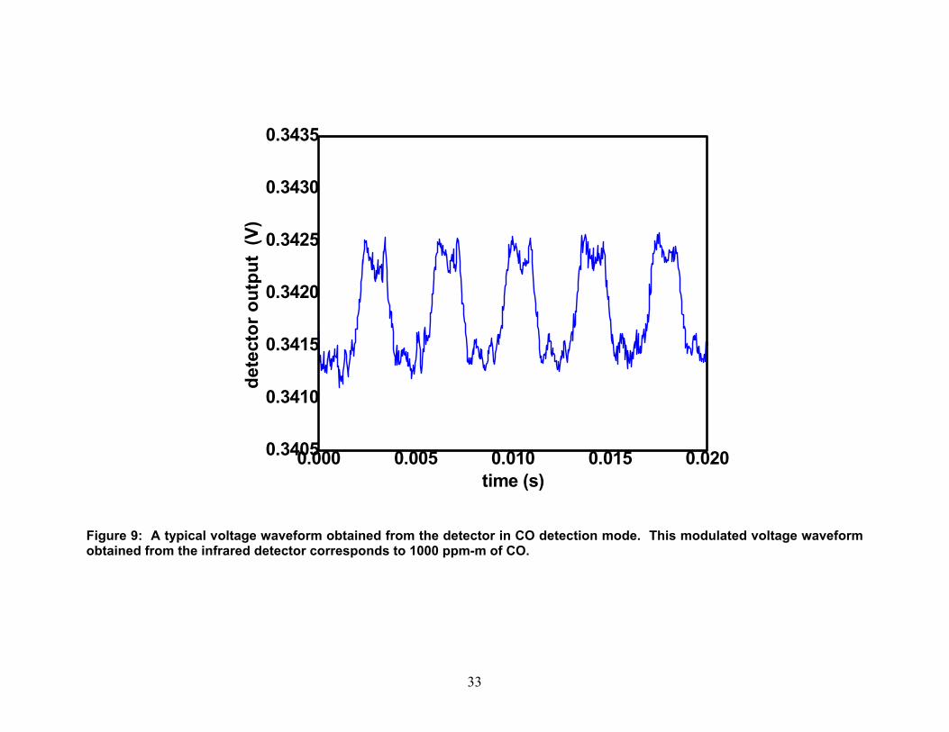
FIGURE 9.: A TYPICAL VOLTAGE WAVEFORM OBTAINED FROM THE DETECTOR IN CO DETECTION MODE. THIS MODULATED VOLTAGE WAVEFORM OBTAINED FROM THE INFRARED DETECTOR CORRESPONDS TO 1000 PPM-M OF CO................................................................................33
FIGURE 10.: THE POWER SPECTRAL DENSITY OBTAINED FROM THE FAST FOURIER TRANSFORM OF THE DETECTOR OUTPUT. THE MAGNITUDE OF THE INTEGRAL OF THE SPECTRAL PEAK IN THE VICINITY OF 260 HZ PROVIDES A MEASURE OR THE CO CONCENTRATION. ........................34
FIGURE 11: PHOTOGRAPH OF “TACHOMETER” CIRCUIT (LEFT) AND THE SYNCHRONOUS DETECTOR CIRCUIT (RIGHT). .....................................................................................................................35
FIGURE 12: SCHEMATIC DIAGRAM OF THE “TACHOMETER” CIRCUIT USED IN THE CO SENSOR. ....36 FIGURE 13: SCHEMATIC DIAGRAM OF DETECTION AND SYNCHRONOUS DETECTOR SECTION OF
DETECTOR CIRCUIT......................................................................................................................................37 FIGURE 14. : SCHEMATIC OF THE LOW-PASS FILTER SECTION OF THE SYNCHRONOUS DETECTION
CIRCUIT............................................................................................................................................................38 FIGURE 15: PLOT OF PEAK TO PEAK AMPLITUDE VS. CONCENTRATION PATHLENGTH FOR CO IN
PURE N2 (OPEN CIRCLES) AND CO IN 11.5% CO2 (FILLED TRIANGLES). DATA ILLUSTRATES THE SYSTEM’S ABILITY TO REJECT SIGNAL FROM CO2 WHILE SIMULTANEOUSLY DETECTING CO. THE NOISE FLOOR IS THE AMPLITUDE OF THE SIGNAL OBSERVED IN A PURE N2 ENVIRONMENT AND REPRESENTS A MEASUREMENT OF THE IMBALANCE BETWEEN THE PLUS AND MINUS EIGEN FUNCTIONS AS A RESULT OF MECHANICAL VARIATION IN THE ROTATION OF THE WHEEL, PROCESS VARIATIONS IN THE MANUFACTURE OF THE MASK WHEEL, SPECTRAL CONTENT OF THE SOURCE LIGHT IN THE WAVELENGTH REGION, AND ERRORS IN THE MASK CALCULATIONS. .................................................................................................39

7
FIGURE 16–: DETECTOR HOUSING MODEL ILLUSTRATING THE OVERALL SIZE AND CONFIGURATION OF THE CONSUMER VERSION OF THIS SENSOR. ALL OF THE OPTICS ARE DIRECTLY MOUNTED TO THE WALLS PROVIDING ROBUSTNESS, SIMPLICITY, AND COST REDUCTION. ...................................................................................................................................................40
FIGURE 17–: GAUGE CAPABILITY EXAMPLE ...................................................................................................41 FIGURE 18–: FMEA EXAMPLE...............................................................................................................................42 FIGURE 19–: GUIDELINES FOR RATING .............................................................................................................43

8
TABLES TABLE 1: PHYSIOLOGICAL RESULTS OF EXPOSURE TO VARIOUS LEVELS OF CO. -------------------------9 TABLE 2: CONDITIONS OF THE FOUR TESTS PERFORMED AT THE CPSC.------------------------------------ 10 TABLE 3: CO AND CO2 VALUES FOR FOUR OPERATIONAL TESTS. CO VALUES ARE IN PPM, CO2
VALUES ARE IN PERCENT-------------------------------------------------------------------------------------------- 10

9
1. INTRODUCTION Carbon monoxide (CO) is a colorless, odorless, and tasteless gas and is a byproduct of the incomplete combustion of fossil fuels such as gas, oil, coal and wood. While CO is an important commercial product used extensively in the oil industry, dangerous amounts of CO may accumulate where poor ventilation is present. This is extremely important in small confined areas such as residential utility spaces. CO poisons people by displacing oxygen in the bloodstream by bonding nearly irreversibly with hemoglobin, therefore, depleting bodily organs of oxygen and causing their subsequent death. Consumers run the risk of CO poisoning from over 15,000 different types of consumer products. Each year there are over 200 deaths caused by CO poisoning and thousands of injuries. The financial impact of CO-related problems (death, injuries, and property damage) totals more than $700 billion annually1.
Concentration of CO in air Inhalation time and toxic developed
50 parts per million (ppm) Safety level as specified by the Health and Safety Executive
200 ppm Slight headache within 2-3 hours
400 ppm Frontal headache within 1-2 hours, becoming widespread in 3 hours
800 ppm Dizziness, nausea, convulsions within 45 minutes, insensible in 2 hours
Table 1: Physiological results of exposure to various levels of CO. In response to this hazard of consumer products, Sandia National Laboratories (SNL) has partnered with the Consumer Product Safety Commission (CPSC) to develop an infrared (IR)-based spectrometer capable of meeting three major requirements. First, the spectrometer must be able to detect sub 100 ppm-meters of CO. Second, this detection must be possible in cases of high background interferents such as carbon dioxide (CO2) and water. Third, the spectrometer design must lend itself to a development path capable of developing small, cheap, and quantitative measuring systems. This final report presents the approach undertaken in developing an analytical tool, meeting these three requirements listed, and the data obtained from this analytical tool.

10
2. BACKGROUND Combustion Byproducts and Their IR Spectra Combustion efficiency of natural gas during furnace operation approaches 100%, with only a small fraction of the original constituents not being broken down into carbon dioxide, water, and other impurities. Figure 1 shows the IR absorbance spectra of combustion byproducts such as CO, CO2, NOx, and SOx. Additionally, the IR absorbance spectra of uncombusted constituents such as methane and ethane are shown. It was the goal of this project to develop a CO monitoring system that was not affected by overlapping spectra, such as CO2 and water (not shown).
Operating conditions within a 92% efficient household furnace were determined by the CPSC. Four operating conditions were tested to (1) provide a baseline of operation (normal) and (2) to mimic the incomplete oxidization of combustion byproducts, leading to elevated CO.
Test 1: Furnace working under overfired conditions. 113.3 kBTU/Hr and normal vent
Test 2: Furnace working under normal conditions. 98.9 kBTU/Hr and normal vent
Test 3: Furnace working under normal conditions. 98.5 kBTU/Hr and blocked vent
Test 4: Furnace working under overfired conditions. 111.0 kBTU/Hr and blocked vent
Table 2: Conditions of the four tests performed at the CPSC.
Below in Table 3 are the quantitative results of carbon monoxide and carbon dioxide testing inside the primary flue of a 92% efficient furnace. Notice, CO and CO2 are greatest under Test 4 conditions. The highest CO2 present in any test was 11.5%. This is important to notice, because CO2 is a possible interferent for CO monitoring. The lowest CO value obtained was 7 ppm.
Test 1
CO
Test 1
CO2
Test 2
CO
Test 2
CO2
Test3
CO
Test 3
CO2
Test 4
CO
Test 4
CO2
Avg 8.92 7.64 10.25 6.52 89.28 9.97 684.70 11.35
Max 10.57 7.7 10.97 6.72 102.32 9.88 791.39 11.44
Min 7.37 7.59 6.86 6.34 65.73 9.05 540.01 11.25
Std. Dev 0.71 0.04 0.49 0.05 8.71 0.11 73.88 0.04
Table 3: CO and CO2 values for four operational tests. CO values are in ppm, CO2 values are in percent
An important part of understanding combustion diagnostics is determining what the IR absorbance spectra of the furnace conditions, particularly under the operating conditions of Test 4. To understand the IR environment of Test 4 the measured furnace conditions were mimicked on a Fourier Transform Infrared (FTIR) spectrometer (Figure 2). Four primary conditions had to be met for successful simulation of Test 4: the matching of CO and CO2 levels, operating temperatures of 212˚F, and 98% relative humidity (RH). This was accomplished by flowing CO and CO2, of appropriate concentrations, through a hot water bath containing a water bubbler, and through a length of tubing wrapped in heat tape. The temperature at the FTIR gas cell was controlled to 212˚F. RH was measured at the end of the flow path using an RH sensor. A 10 cm long gas cell was used for all measurements.

11
Multiple experiments were run for all testing conditions stated in Table 2. The most comprehensive test ran on the FTIR comprised 500 ppm CO and 11.5% CO2, 225˚F, and 93% RH. While these conditions are not exactly the same as those present under Test 4, they were the closest simulation that could be accomplished outside of an actual furnace. Notice that the two CO peaks (represented by humps) and CO2 absorbance line in Figure 3 do not show much interference with CO absorbance lines. Water absorbance lines provide the largest interference with CO absorbance lines under Test 4 conditions.
Furnace Integration To test the spectrometer under actual conditions, a 92% efficient furnace (Figure 4) was purchased. The spectrometer is to be integrated onto the secondary flue of the heat exchanger (circled in yellow). The secondary flue is where the combustion by-product water drain pan is located indicating an expected high humidity level in this region. The spectrometer will be integrated onto the side of the furnace and the optical path for the spectrometer passes through the length of the secondary flue and is reflected back via a mirror. This double pass arrangement allows for a 36 inch (0.914 m) long detection pathlength.
Spectrometer Design Figure 5 shows a schematic layout of the rotating mask spectrometer used for measuring the infrared transmission spectrum of the sample volume. Infrared radiation from a resistively heated element is collimated using a CaF2 lens and directed through a 10 cm path-length sample volume. The transmitted radiation is then focused by a second CaF2 lens through the entrance slit of the spectrometer. An off-axis parabolic mirror collimates the light emerging from the entrance slit and directs it onto a 150 groove/mm diffraction grating. The spectrally dispersed light is then focused by a ZnSe lens. A turning mirror serves to reduce the overall dimensions of the optical package. The first mirror of a periscope assembly is used to redirect the infrared radiation so that it passes vertically (i.e. perpendicular to the base-plate) through the mask wheel. The plane of focus of the infrared radiation is adjusted to precisely coincide with the metallic patterns fabricated on the mask wheel. After being filtered by the mask pattern, the remaining radiation is redirected by the second mirror of the periscope assembly such that it once again travels parallel to the base-plate. The infrared radiation is returned along the incident path, reflecting off the turning mirror and passing through the focusing lens. The diffraction grating recombines the remaining spectral components, which are the focused by the off-axis parabolic mirror. The returning beam is slightly displaced vertically due to the periscope assembly, and a small pick-off mirror is used to direct the focused radiation onto the HgCdTe infrared detector (Figure 6).
To measure the infrared transmission spectrum of the sample volume, the mask wheel is positioned so that the position of the spectrally dispersed infrared light coincides with the position of the Hadamard masks fabricated along the outer periphery of the mask wheel (Figure 7). As the wheel rotates, the Hadamard masks are sequentially positioned in the infrared beam and the intensity corresponding to each mask is recorded. The synchronization pattern fabricated near the center of the mask wheel, in conjunction with the synchronization electronics ensure that the detector output for each mask can be identified. The sequence of Hadamard weights can then be inverted using standard Hadamard techniques to recover the infrared spectrum.
For CO detection, the grating wheel is moved laterally until the position of the detection masks coincides with the position of the focused, spectrally dispersed, infrared light. Rotation of the mask wheel causes the “plus” and “minus” masks to be alternately placed at the position of the

12
beam (Figure 8). The detector output is continuously recorded. The voltage waveform usually exhibits a square-wave like appearance due to the differences in transmission through two types of masks (Figure 9). A Fast Fourier transform is applied to the voltage waveform to determine the amplitude of modulation, which provides a measure of the concentration path-length product of the CO gas (Figure 10).
Mask Wafer design Figure 7 shows a circular mask wheel. This mask wheel can be reflective or transmissive in nature. For the spectrometer designed above, the mask was used in the transmissive state. The mask wheel incorporates three radial regions; in the center is a radial region of position fiducial markers for monitoring the mask position; in the middle of the wafer are repeated A-B pairs of chemical species-specific masks, called Eigen masks (Figure 8); on the outer edge of the wafer are Hadamard masks. The position fiducial markers comprise an alternating series of metallization (reflectance) and no metal (transmission) patterns. This synchronization region of the mask wheel is read by an optical reflectance circuit and used by the synchronous detector to associate each photo-detector measurement with the particular mask that is illuminated at that instant. The wheel is mounted onto a flat chuck that holds the wafer in place by vacuum. The wafer is turned at a desired rotation rate using a precision motor.
The IR spectrometer incorporated two methods of detection. The first method, using Hadamard masks, contains a series of masks for a given span of spectral region. These masks contain transmission and reflectance portions that block undesired light bands, while allowing light in desired bands to be detected by a photo-detector. The results of detector output are used to yield a spectral representation (such as the results obtained through FTIR). The second method was designed to contain a series of species-specific masks (Eigen masks) that likewise possess transmission and reflectance portions that block undesired light bands, while allowing desired light bands to pass onto a photo-detector. Both of these mask sets are fabricated onto a silicon wafer using standard photolithography.
Eigen gratings defined Eigen masks can be designed for reflective or transmissive operation. In work for the CPSC, transmissive Eigen mask are used to determine the presence of a chemical by employing a priori knowledge of the transmission spectra of the target species. For the case of CO detection, the eigen masks can be designed empirically. The CO absorption spectrum in the vicinity of 2150 cm-1 consists of a regular sequence of narrow absorption peaks. In this case, two masks may be designed such that the first mask contains a sequence of transmissive windows that precisely overlap the absorption peaks of the CO spectrum. The second mask contains a similar sequence of windows, however in this case the sequence is shifted slightly so that they overlap the “valleys” between the peaks of the CO spectrum. Thus, if a sample with significant CO is present, the spectrally integrated transmission obtained using the first mask will be smaller than that obtained with the second mask, and a modulation signal will be observed.
In more complex situations, a mathematical algorithm can be employed to determine the optimal mask set which maximizes the response to the species of interest, while simultaneously minimizing the response of the system to spectrally interfering compounds, such as water (Figure 3). This approach leads to a matrix equation that is solved for the appropriate reference spectra using Singular Value Decomposition (SVD). The SVD method is very general. It assumes that two spectral masks will alternately be placed in the beam, but does not assume that one mask is (B) (B)

13
simply a shifted copy of the other. In general, the two masks bear very little resemblance to one another2, 3, 4.
To formulate a mathematical description of the sensing mask, a given a set of target species (A,B,C…) is assumed that are potentially present in a sample volume, and an input radiance spectrum is assumed. The set of reference spectra (a+, a-, b+, b-…) is determined that optimizes the selectivity of correlation-based sensing of these species. When probing for species A, the radiometer will alternately produce the reference spectra a+ and a-, and the modulation of the spectrally integrated intensity reaching the detector will be measured. In a similar manner, reference spectra b+ and b- are used to detect species B. Ideally, each pair of reference spectra will produce a modulation signal only if the target species for which the pair was designed is present. The input sample spectrum is given by
( ) ( ) ( ) ( )0 a bL A c B cI I e ν νν ν − ⋅ ⋅ + ⋅ +⎡ ⎤⎣ ⎦= ⋅ L (1)
where L is the sample path-length, A(v) and ca are the absorption spectrum and concentration of species A. For small concentrations where the exponent is a small number, Eq. (1) can be approximated as:
( ) ( ) ( ) ( ) ( ) ( )0 0 0a bI I I A c L I B c Lν ν ν ν ν ν= − ⋅ − ⋅ −L (2)
The reference spectra a+ and a- for the detection of species A should satisfy the following integral equations:
( ) ( ) ( )
( ) ( ) ( ) ( )
( ) ( ) ( ) ( ) ( ) ( ) ( ) ( )
2
1
2
1
2 2
1 1
0
0
0 0
0
0
0
A
d I a a
d I A a a S
d I B a a d I C a a
ν
ν
ν
ν
ν ν
ν ν
ν ν ν ν
ν ν ν ν ν
ν ν ν ν ν ν ν ν ν ν
+ −
+ −
+ − + −
⎡ ⎤− =⎣ ⎦
⎡ ⎤− = ≠⎣ ⎦
⎡ ⎤ ⎡ ⎤− = − = =⎣ ⎦ ⎣ ⎦
∫
∫
∫ ∫ L
(3)
These equations simply state that, when reference spectra a+ and a- are used, a signal should only be generated if species A is present. Likewise a similar set of equations can be written for species B etc.
These equations can be written in discrete form as
0
0
0 0
0
0
0
i ii
Ai i i
i
i i i i i ii i
I a
I A a S
I B a I C a
⋅ =
⋅ ⋅ = ≠
⋅ ⋅ = ⋅ ⋅ = =
∑
∑
∑ ∑
%
%
% % L
(4)

14
where the “Eigenspectrum” for species A has been defined as
i i ia a a+ −≡ −% (5)
In matrix form, these equations become:
0 0 011 2
0 0 021 1 2 2
0 0 031 1 2 2
0 0 01 1 2 2
0
0
0
NA
N N
N N
N N
N
aI I Ia SI A I A I AaI B I B I B
I C I C I Ca
⎛ ⎞⎛ ⎞ ⎛ ⎞⎜ ⎟⎜ ⎟ ⎜ ⎟⎜ ⎟⎜ ⎟ ⎜ ⎟⎜ ⎟⎜ ⎟ ⎜ ⎟=⎜ ⎟⎜ ⎟ ⎜ ⎟⎜ ⎟⎜ ⎟ ⎜ ⎟
⎜ ⎟⎜ ⎟⎜ ⎟ ⎝ ⎠⎝ ⎠⎝ ⎠
%L
%L
%L
M ML
%M O
(6)
Similarly for species B:
0 0 01 2 1
0 0 01 1 2 2 20 0 01 1 2 2 30 0 01 1 2 2
00
0
N
N NB
N N
N N
N
I I I bI A I A I A b
SI B I B I B bI C I C I C
b
⎛ ⎞⎛ ⎞ ⎛ ⎞⎜ ⎟⎜ ⎟ ⎜ ⎟⎜ ⎟⎜ ⎟ ⎜ ⎟⎜ ⎟⎜ ⎟ ⎜ ⎟=⎜ ⎟⎜ ⎟ ⎜ ⎟⎜ ⎟⎜ ⎟ ⎜ ⎟
⎜ ⎟⎜ ⎟⎜ ⎟ ⎝ ⎠⎝ ⎠⎝ ⎠
%L%L%L
ML M%M O
(7)
It is not possible to obtain explicit solutions to these matrix equations, since they involve more unknowns than equations. However, it is possible to obtain the best solution (in a least-squares sense) using SVD, and back-substitution. To do this, the coefficient matrix is padded with rows of zeros to form a square matrix, SVD is applied, and back-substitution is employed to obtain the difference spectrum. This procedure is repeated to obtain the Eigenspectrum for each target species. Using this method, multiple Eigen A-B pairs (representing a unique cross-correlation) can be fabricated along the circumference of the mask wheel. For example, using a five-inch-diameter silicon wafer as the mask wheel, up to 71 discrete compounds can be measured using this method.
Hadamard gratings defined The outer region of the mask wheel comprises Hadamard masks to measure the transmission of spectra from a given sample. The Hadamard pattern is formulated wherein each pattern represents about 360º/n of arc for an n-bit Hadamard pattern. For example, in its current design, the Hadamard mask-set is comprise of 283 adjacent segments. Adjacent Hadamard masks comprise the same mask architecture; however, a cyclic permutation by one segment is performed for each new adjacent mask. This process is repeated 283 times, until the cycle is complete. To measure a spectrum, the incoming light is sequentially filtered with each of the Hadamard masks, and the photo-detector output is recorded. An inverse transformation procedure is then employed to recover the spectrum of the incoming light from the ensemble of photo-detector measurements. Using this method, one obtains the transmission or emission spectrum of the gas to be analyzed5.
Electronics The electronics constructed for the application consisted of two circuits each with different functionality. The “tachometer” (Figure 11 and Figure 12) is based on an Agilent HEDS-1500
15
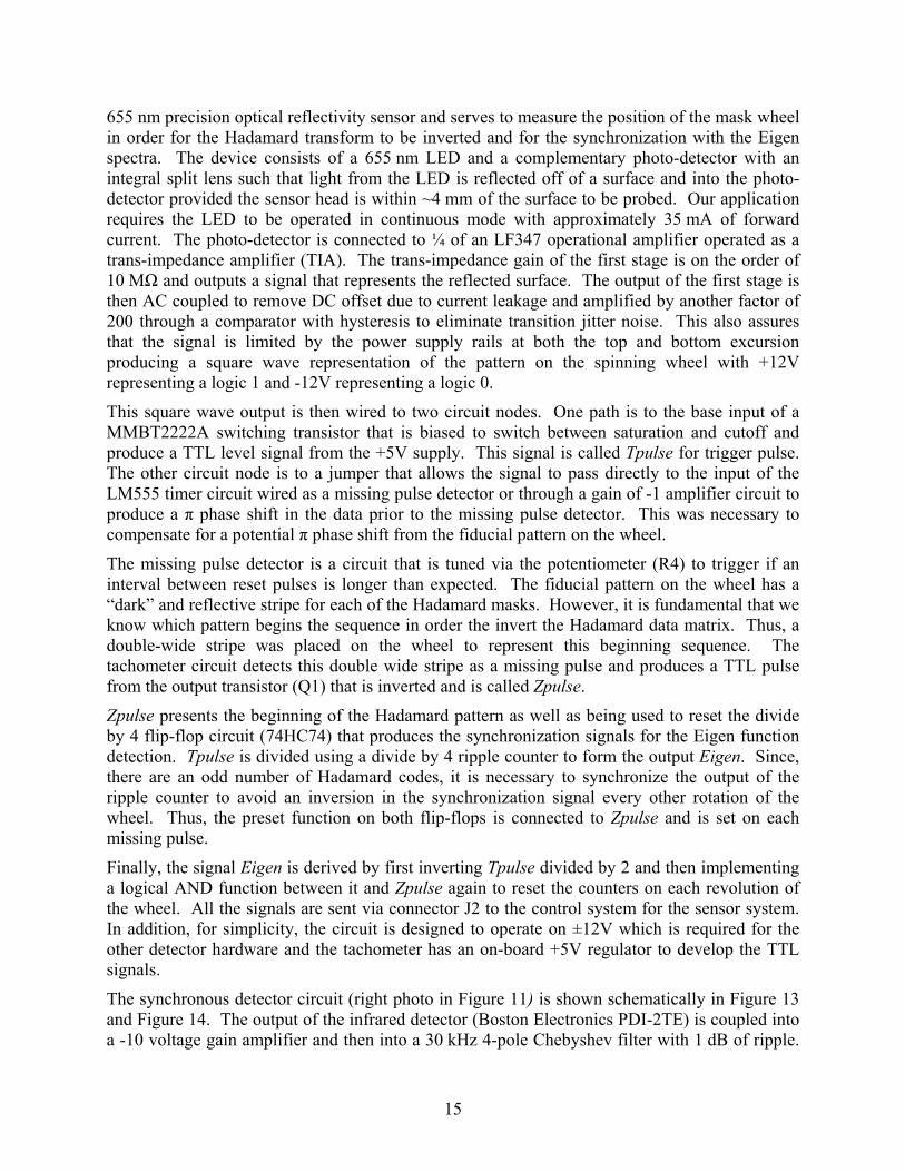
655 nm precision optical reflectivity sensor and serves to measure the position of the mask wheel in order for the Hadamard transform to be inverted and for the synchronization with the Eigen spectra. The device consists of a 655 nm LED and a complementary photo-detector with an integral split lens such that light from the LED is reflected off of a surface and into the photo-detector provided the sensor head is within ~4 mm of the surface to be probed. Our application requires the LED to be operated in continuous mode with approximately 35 mA of forward current. The photo-detector is connected to ¼ of an LF347 operational amplifier operated as a trans-impedance amplifier (TIA). The trans-impedance gain of the first stage is on the order of 10 MΩ and outputs a signal that represents the reflected surface. The output of the first stage is then AC coupled to remove DC offset due to current leakage and amplified by another factor of 200 through a comparator with hysteresis to eliminate transition jitter noise. This also assures that the signal is limited by the power supply rails at both the top and bottom excursion producing a square wave representation of the pattern on the spinning wheel with +12V representing a logic 1 and -12V representing a logic 0.
This square wave output is then wired to two circuit nodes. One path is to the base input of a MMBT2222A switching transistor that is biased to switch between saturation and cutoff and produce a TTL level signal from the +5V supply. This signal is called Tpulse for trigger pulse. The other circuit node is to a jumper that allows the signal to pass directly to the input of the LM555 timer circuit wired as a missing pulse detector or through a gain of -1 amplifier circuit to produce a π phase shift in the data prior to the missing pulse detector. This was necessary to compensate for a potential π phase shift from the fiducial pattern on the wheel.
The missing pulse detector is a circuit that is tuned via the potentiometer (R4) to trigger if an interval between reset pulses is longer than expected. The fiducial pattern on the wheel has a “dark” and reflective stripe for each of the Hadamard masks. However, it is fundamental that we know which pattern begins the sequence in order the invert the Hadamard data matrix. Thus, a double-wide stripe was placed on the wheel to represent this beginning sequence. The tachometer circuit detects this double wide stripe as a missing pulse and produces a TTL pulse from the output transistor (Q1) that is inverted and is called Zpulse.
Zpulse presents the beginning of the Hadamard pattern as well as being used to reset the divide by 4 flip-flop circuit (74HC74) that produces the synchronization signals for the Eigen function detection. Tpulse is divided using a divide by 4 ripple counter to form the output Eigen. Since, there are an odd number of Hadamard codes, it is necessary to synchronize the output of the ripple counter to avoid an inversion in the synchronization signal every other rotation of the wheel. Thus, the preset function on both flip-flops is connected to Zpulse and is set on each missing pulse.
Finally, the signal Eigen is derived by first inverting Tpulse divided by 2 and then implementing a logical AND function between it and Zpulse again to reset the counters on each revolution of the wheel. All the signals are sent via connector J2 to the control system for the sensor system. In addition, for simplicity, the circuit is designed to operate on ±12V which is required for the other detector hardware and the tachometer has an on-board +5V regulator to develop the TTL signals.
The synchronous detector circuit (right photo in Figure 11) is shown schematically in Figure 13 and Figure 14. The output of the infrared detector (Boston Electronics PDI-2TE) is coupled into a -10 voltage gain amplifier and then into a 30 kHz 4-pole Chebyshev filter with 1 dB of ripple.

16
This is to allow both Eigen mask-derived and Hadamard mask-derived electrical signals to pass at all of the projected wheel rotation speeds. This signal is directly available for analog-to-digital conversion at J4 labeled Output.
This signal is also directed to the input of an AD630 precision balanced modulator/demodulator. The AD630 is wired to act as a synchronous detection circuit that has a switchable gain from +1 to -1. The gain select is controlled by the input called SYNC and is connected to the signal called Eigen2 from the “tachometer” circuit. The signal Eigen2 is designed to have a logic level high for a particular Eigen code and then switch to logic low for the adjacent Eigen code such that alternating codes are represented by logic high for the positive Eigen function and a logic low for the negative Eigen function. As there are minor phase shifts possible due to phase lag in the amplifier and filter circuits, we have included a method of adjusting the phase to compensate. The fine phase shift is accounted for by the operational amplifier circuit U5D and the series of jumpers for coarse (π) phase shifts. By adjusting the phase, a full-wave rectified signal that is synchronous with the Eigen codes is passed through the AD630 while noise signals that are not of the same phase and frequency of the Eigen codes are averaged to zero. Since the full-wave signal has a non-zero average if CO is present, the output of the detector is coupled into a MAX7480 8-pole switched capacitor low-pass Butterworth filter. This low-pass filter outputs a DC voltage that is proportional the amplitude of the modulation signal. Since the modulation is proportional to the correlation of the light with the Eigen function, the DC level is proportional to the concentration of the CO in the sample.
The MAX7480 is tuned by the control signal derived from the LM555 (U4) wired to operate in bi-stable mode and adjustable via the potentiometer (R1). The corner frequency of the low-pass filter is fixed by the frequency of the output of the LM555 which must be 100 times larger than the desired corner frequency. Since the rotational frequency of the wheel was not precisely known when this section was designed, it was necessary to implement a tunable filter for the system. An issue coupled to the switched filter is transient noise at the oscillator frequency. Thus, analog low-pass “anti-aliasing” filters are required at the output of the MAX7480 and these are implemented using a 4-pole low-pass Butterworth design with a corner at 100 Hz as depicted from U2B and U2C in Figure 14. The 100 Hz anti-aliasing filter allows the switched filter to operate down to 1 Hz giving the synchronous detector circuit and overall time constant of 1 sec.

17
3. DATA Laboratory Detection of Carbon Monoxide Testing of the system under various conditions was undertaken including measurement of pure CO in background N2. The samples were prepared using a mass flow system that is computer controlled to develop a calibrated gas stream and then flowing that stream into a 10 cm long vessel with CaF infrared windows. The gas was allowed to flow through the cell at 1 slm) until a minimum of 10 volumes of gas had passed through the cell to flush out the previous sample. This allows confidence in the CO concentration in the cell. The cell was then transported from the gas handling laboratory to the optical laboratory and placed in the IR beam to be imaged by the detection system. Various concentrations of CO were tested and the results are illustrated as the open circles in Figure 15. Figure 15 is a plot of the square root of the integral area under the power spectrum curves (Figure 10) as found from a Fast-Fourier Transform (FFT) of the sampled data. The solid line is a fit of the data to a function of the following form where Vp-p is the signal and C is the concentration of CO in ppm.
( )1 Cp p oV V V e λ−
− ′= + − (8)
where Vo is a DC offset to compensate for DC errors in the detection system and has a value of -2.34x10⁻⁵ V, V’=1.25x10⁻³ V, and λ=1.69 x10⁻³ ppm-1-m-1. The value of V’ is a measure of the maximum signal amplitude that can exist in the sensor and is a function of the absolute gain of the detection electronics. However, its physical meaning is that CO will absorb light of certain characteristic wavelengths during its passage through the sample cell. When the concentration is high enough that no more light at those characteristic wavelengths remains to be absorbed the difference between the two Eigen functions measured in volts is V’. Finally, λ is a sensitivity constant that represents the aggregate absorption of CO over the entire wavelength band. The line in Figure 15 labeled “noise floor” was determined by integrating the power spectrum with pure N2 in the cell and represents the value of Eigen function mismatch due to rotation of the wheel, process variations in the manufacture of the mask wheel, structure in the source spectral radiance, and errors in the mask calculations. As observed in Figure 15, the limit of CO detection (signal-to-noise equal to 1) is approximately 20 ppm-m – a value well below the minimum safe concentration quoted in Table 1.
Laboratory detection of CO in 11.5% CO2 Similar measurement samples were prepared and tested using the system that included a concentration of background CO2 representative of values expected (11.5%) during combustion of natural gas in a furnace. Again, the flow cell was flushed and backfilled as described above and placed in the IR beam. This data is represented by the blue inverted triangles plotted in Figure 15. As observed the data has no discernable variation from the samples in pure N2 indicating that CO2 is not measured by the system. Referring back to Figure 1 and Figure 3, we observe that CO2 has a substantial absorption very near the wavenumber region of interest but is not observed by the radiometer. This is a result of the rejection capability of the Eigen spectrum approach and illustrates its power as an optical measurement technique in systems with many components whose spectra overlap!

18
4. ROADMAP TO COMMERCIALIZED CONSUMER PRODUCT In order for this technology to move from a laboratory proof of concept to a commercialized consumer product, a market will need to exist. A market will exist if the consumer perceives or achieves a benefit that is greater than the cost expended for this product resulting in some amount of value. The benefit of this product lies in the improved efficiency of the furnace and additional safety measures provided, the cost will be determined through the commercialization process. Cost numbers less than $20 have been suggested but only the manufacturers and consumers truly know what an acceptable cost is.
To commercialize this laboratory proof of concept, a number of actions will have to occur or at least be considered. These actions when performed in a sequence make up a possible roadmap to a consumer product. Of course there are many paths that can lead to the same commercialization result, and these paths are unique to each particular entity trying to create the consumer product. An example roadmap with only the significant actions required is discussed in this section. The detailed actions will be left to the commercializing entity.
Example roadmap: 1) Size Reduction and Packaging
2) Gauge Capability
3) Failure Mode and Effects Analysis
4) Design for Manufacturability Analysis
Two results that typically fall out from these actions will be lower cost and greater reliability. Then, along with a corresponding market demand (which tends to increase as cost goes down and reliability goes up), this technology can emerge as a low cost, high volume, reliable consumer safety product that is incorporated into furnaces nationwide.
Size Reduction and Packaging The current laboratory proof of concept has many components that will not be necessary as a consumer product. For example, the rotating wheel and all of its associated components, (i.e. motor, electronics for RPM control, mounting hardware, etc.) will not exist in the consumer product version. In fact, the consumer product will be solid state. These other components were used in the development to learn what is required for the solid state design. As a result, the package will be completely different and the size will reduce significantly. The resulting size reduction will give way to few parts and less raw material resulting in a lowered cost and greater reliability.
Figure 16 shows a model of the detector housing as envisioned for the consumer product. This housing would mount to the side of the furnace such that the spectral sample would enter the housing as shown. The sample would then pass through a number of optics manipulating the sample for the detector located inside the housing. The sample would eventually reach the photo- detectors located in the middle of the housing.
The detector would actually be an array of photo-detectors with at least two individual photo-detectors for each sample of combustion byproduct targeted for monitoring. For example, if CO and CO2 are targeted, a total of four photo-detectors would make up the photo-detector array. The photo-detectors would be solid state with a metal filter deposited over them using semiconductor processes. The metal filter would be a spectral filter that would be a result of

19
what was learned from the Hadamard transform and Eigen studies obtained from the spinning wheel. A photo-detector array with the spectral filter deposited over it could be produced in one process from the manufacturer of the photo-detector as a custom device. As custom semiconductor processing is expensive, pricing for this custom device would be heavily dependent on the quantity purchased.
The housing can be mass produced using injection molding manufacturing techniques, and the optics in the detector housing could be mass produced and/or built into the housing itself further reducing cost. The material for the housing and the optics will not need to stand up to a harsh environment since it is located outside of the combustion region. The reflective coatings for the optics could be applied after the housing is made further reducing cost.
Finally, the output of the sensor unit would be signals representing the concentration of the combustion by-products. These signals could be connected to the controller of the furnace to make incremental adjustments to the fuel/air input for maximum efficiency or shutdown the furnace entirely in the case of unsafe concentrations.
Gauge Capability After the laboratory proof of concept has been reduced and packaged into a consumer product, a study regarding the performance is necessary to understand the true performance of the product. The product is essentially a sensor, and sensors must be accurate (calibrated) and precise (capable) if they are to provide useful information.6. Generally, accuracy is easier to accomplish than precision. Provided enough signal-to-noise ratio exists, accuracy can be achieved by calibrating or characterizing the sensor to a known concentration(s). The precision or capability is a function of the variation in the readings when making the same measurements repeatedly. Sensor variation typically shows up in uncontrolled variables within the sensor. In this product, uncontrolled variables could be something as simple as the temperature variation wherever the furnace is located since the detector housing would be mounted to the furnace. Another example of an uncontrolled variable would be the cleanliness of the optics or window through which the probe light passes. To characterize and understand the performance of the product, a sensor capability study would be required.
A sensor capability study is illustrated in the spreadsheet shown in Figure 17. The spreadsheet shows three different trials of ten samples made by three different operators. The measurement values are placed in the spreadsheet where statistics are calculated on the data in order to determine the capability for the measurement system and the variation contribution of the operator. Definitions of the columns are given below.
O/A tolerance = Tolerance desired to be measured to.
X_Bar = Average of 30 measurements for each operator
X_Diff = Max – Min of X_Bars
R_Bar = Max – Min for each operator out of 30 total measurements
R_Bar2 = Average of the three ranges
K1=3.55 and K2=3.14 are statistical constants used for three trials.
n*t = Total number of samples
Gauge variation = (R_Bar2)*K1 / Tolerance

20
Operator variation = ((X_Diff*K2)2 – (Gauge Variation)2 )1/2 / Total Samples / Tolerance
Total Repeatability and Reproducibility (R&R) = Vector summation of Gauge and Operator Variations.
For minimal acceptable performance, the total R&R should be less than 30%. Note that as the tolerance is increased, the sensor becomes more acceptable. This makes intuitive sense in that if the tolerance requirement is relaxed by some amount, the sensor will become more acceptable. For example, if the perimeter of a building was required to be measured to the nearest inch and the gauge is a 12” ruler with no markings on it, the gauge would not be very acceptable. However, if the requirement was relaxed so that the perimeter was to be measured to the nearest 10 feet, then the 12” rule with no markings on it would be more acceptable. This concept is important in that no matter how well the sensor performs; an acceptable tolerance level can be found. If the tolerance level to which the gauge is specified is not acceptable to the user, improvement in the sensor design must be explored.
Gauge capability is a common tool used in the manufacturing and assembly industries. Most statistical software packages have this capability built into them. There are different techniques with the statistical analysis behind the tool, but the general idea is basically the same. Reducing the variation in your readings due to establishing control of the uncontrolled variables will lead to an improved gauge.
Failure Mode & Effects Analysis (FMEA) Failure Mode and Effects Analysis is a technique used for advanced product quality planning, problem solving, or continual improvement that can be applied to either product design or manufacturing and assembly processes. The application of an FMEA to product design and production can significantly reduce the number of failures associated with a product throughout its life-cycle.
The concept of identifying and preventing potential product failures originated in the late 1940s and early 1950s when technology began advancing at a pace that exceeded product reliability. First applied to the aerospace industry during the early days of the space program, NASA engineers needed a way to help them anticipate every conceivable malfunction. As a result, they developed a structured brainstorming approach that became known as the Failure Mode and Effects Analysis (FMEA).7
The FMEA concept is applicable to any industry or product. As the engineers from the aerospace industry moved into other industries, they brought with them the FMEA tool, and as a result, its use became more widespread. However, it was the automotive industry that really applied the FMEA to consumer products in its endeavor to improve quality in the face of Japanese competition. Because of this, the automotive method for applying the FMEA is what is generally applied to consumer products.
An example FMEA is shown in Figure 18. The FMEA can be broken down into four important sections, each highlighted in a different color: 1) Potential Failures in blue, 2) Potential Causes in yellow, 3) Current Design Evaluation and Control in green and 4) Risk Priority Number (RPN) with associated improvement actions.
1) Assessing potential failures (blue): Beginning at the left of the example, for each functional product requirement, the design team will brainstorm the potential failure modes. For each potential failure mode, the team will then

21
brainstorm the potential failure effect. For each effect, a severity will be assigned. The severity is a ranking from 1 to 10 of the severity of the problem with 10 being the most severe. Figure 19 provides guidelines of how to rate severity for a consumer product. In general, a rating of 10 is considered the most severe and is reserved for injury or death due to a product failure while a rating of 1 is considered a minor inconvenience. In the simple example shown in Figure 18, the functional product requirement is analysis of the spectrum and the failure mode is a broken detector wire resulting in a no reading failure effect. The severity level was classified as 8 due to a loss of primary function.
2) Assessing potential causes (yellow): The chart is continued by moving to the right where all potential causes for a failure mode are then brainstormed by the team. These causes are then ranked with an occurrence rating of 1 to 10. Again, Figure 19 provides guidelines of how to rate the occurrence level for a product failure cause. For the example cited, the cause was a pinched wire during installation. This is considered an occasional moderate failure and was therefore assessed a 4.
3) Assessing current control: Again, the chart is continued by moving to the right where the ability of the design to monitor and control a particular failure is assessed. The design control for each failure mode is listed and then assessed according to the ability of the design to detect the failure. The ranking for detection is also a scale from 1 to 10, but in this case, a ranking of 1 is a strong ability for the design to detect and control the failure whereas a 10 would mean that the design has no visibility to a failure. Our example assumes that the design would have a self-test at start up that would measure known levels of CO or CO2. This is almost certain detection so it was assessed a 1.
4) Risk Priority Number with Improvement Actions: The fourth category is Risk Priority Number or RPN with improvement actions. This is simply the product of all ratings. A good rule of thumb is that an RPN greater than 100 would merit some sort of action to improve the design making it less likely to fail. These actions are recorded on the far right side of the table with new assessments after the improvement has been implemented.
The FMEA is a valuable tool used to try and predict failures before they happen and incorporate improvements into the design. A good FMEA will result in vastly improved reliability in a consumer product that is required to function for more than 20 years. As with the gauge capability study, there is a lot of information available about FMEAs with a quick search on the internet. They should be performed by the commercializing entity’s design team as they would be most intimate with the design.
Design for Manufacturability Assessment When a product is considered high volume and low cost as this one would be, design for manufacturability becomes increasingly important. Design for manufacturability implies that the design incorporates key features that make the product easy to manufacture. Some basic concepts are:
• Designs that cannot be misassembled (i.e. incorporating keyed connectors and color coded wires)
• Designing to eliminate or reduce known or anticipated failure modes (FMEA) • Design for reliability (FMEA) • Design for minimal parts

22
• Design for common parts • Design to factory’s tolerance capability • Designing for competitive advantage (improved productivity – minimize non-value
added activities) • Incorporate test ports for easy diagnosis • Designing for maintainability
Many of these concepts seem obvious but are sometimes glossed over leading to missed opportunities for lower costs. Whatever entity commercializes this technology will eventually need to assess the manufacturability according to their standards and processes in order keep costs low and reliability high.
In summary, a market will exist for a product if the perceived or achieved benefit is greater than the total cost resulting in some sort of value. This technology offers a benefit in improving efficiency and adding another layer of safety to the home furnace industry. The challenge will be to keep the cost low enough such that value is achieved. This section presented a high level roadmap for commercializing this technology that will help keep costs low and reliability up. The roadmap began by discussing a proposed size reduction and packaging concept. From there, prototypes can be built and assessed with the use of a gauge capability study. Somewhere in the process a FMEA should be performed to try and anticipate failures both in the manufacturing process and out in the field. The FMEA will lead to greater reliability and customer satisfaction. Finally, as the design of the product is progressing, a design for manufacturing assessment should be made that incorporates concepts that can improve the overall manufacturing process. Any commercial entity or entities that choose to purse this opportunity will be faced with a number of challenges that can be overcome. Following a good roadmap to bring this technology from laboratory concept to consumer product should ease some of these challenges and hopefully pay large dividends in the end.
23
5. CONCLUSIONS We have demonstrated a laboratory instrument based on a rotating mask spectrometer where transmission masks alternate between a positive going synthesized Eigen spectrum and a negative going synthesized Eigen spectrum. The optical design is explored in detail including the manufacture of the rotating mask. In addition, designs for the required electronic hardware to allow synchronization of the mask rotation with the analog-to-digital converter data signals is provided. The electronics allow monitoring of the mask rotation allowing inversion of the Hadamard spectrum as well as correlation of the optical signal with the positive and negative Eigen spectra integrated signal.
The system was tested under laboratory conditions with CO contamination in a background of pure N2 and with CO2 as a substantial component interferent. The system was found to have no measurable response difference with the interferent demonstrating the power of the Eigen function technique in multi-component systems where spectral overlap is substantial.
Finally, we have designed a conceptual package for a feasible spectrometer that could be manufactured for home and commercial furnace applications. Using rapid prototyping techniques a mockup enclosure was fabricated to demonstrate the feasibility of the design. In addition, we have discussed, at a high level, how a validation program could be implemented on this type of sensor system.
Sandia is a multiprogram laboratory operated by Sandia Corporation, a Lockheed Martin Company for the United States Department of Energy’s National Nuclear Security Administration under contract DE-AC04-94AL85000.

24
6. REFERENCES 1 http://www.cpsc.gov/cpscpub/pubs/466.html. 2 W. H. Press et al., Numerical Recipes in C: The Art of Scientific Computing, Second Edition,
Chap. 2, Cambridge University Press, New York, NY, 1997). 3 M. B. Sinclair et al., “A MEMS-Based Correlation Radiometer,” Proc. IEEE 5346, 37 (2004). 4 K. B. Pfeifer, M. B. Sinclair, Sixth Joint Conference on Standoff Detection for Chemical and
Biological Defense, October, 25-29, 2004 in Williamsburg, VA. 5 M. Harwit and N. J. A. Sloane, Hadamard Transform Optics, Chapters 1-3, Academic Press,
(1979). 6 W. A. Levinson and F. Tumbelty, SPC Essentials and Productivity Improvement: A
Manufacturing Approach, Chapter 5, ASQC Quality Press, (1996). 7 Technicomp, Inc., Failure Mode & Effects Analysis Instructor’s Guide, Unit 1, Overview,
Technicomp, (1995).

25
Figure 1: IR absorbance of combustion products and byproducts possible during the operation of a furnace under various conditions.

26
Bubbler
Hot water bath
Drip line Gas Chamber FTIR
RH Sensor
Figure 2: Setup of FTIR experiments to measure IR spectra that are simulations of that found in a fully operating furnace under various conditions.

27
Water absorbance bands
CO CO
Figure 3: IR spectra obtained through FTIR analysis of furnace under Test 4 operating conditions.

28
Hole cut in paneling for spectrometer access
Figure 4: Photograph of modifications made to a residential furnace that allows installation of the spectrometer.

29
entrance slit IR source
off-axis paraboloid
conventional diffraction grating
focusing lens turning mirror
detector mask wheel
motor
periscope assembly
Figure 5: A schematic layout of the rotating mask spectrometer/CO detector illustrating the optical components and showing the ray trace through the system.

30
Figure 6: A photograph of the optical assembly used for the measurements showing the optical components, rotating disk, and the optical detector.
Rotating Disk
HgCdTe Detector

31
Figure 7: (A) a close up of the specific grating regions and their design. (B) a photograph of a complete 5-inch diameter wafer.

32
2100 2150 22000.0
0.9
1.8
2.7
mas
k tra
nsm
issi
on
wavenumbers
P=3.29e-7 W
P=3.37e-7 W
ΔP=8e-9W
2100 2150 22000.0
0.9
1.8
2.7
mas
k tra
nsm
issi
on
wavenumbers
P=3.29e-7 W
P=3.37e-7 W
ΔP=8e-9W
Figure 8: An Eigen A-B mask set as a function of wavenumber position. Mask set A (Blue) blocks the absorption peaks of CO (Black lines in middle) and is referred to as the “plus” mask. Mask set B (Red) blocks the absorption valleys of CO and is referred to as the “minus” mask. As the disk rotates, the spectra (Black) is alternately filtered by each Eigen spectra resulting in a modulated signal similar to Figure 9.
33
0.000 0.005 0.010 0.015 0.0200.3405
0.3410
0.3415
0.3420
0.3425
0.3430
0.3435
dete
ctor
out
put
(V)
time (s)
Figure 9: A typical voltage waveform obtained from the detector in CO detection mode. This modulated voltage waveform obtained from the infrared detector corresponds to 1000 ppm-m of CO.

34
150 200 250 300 350 400
0.0000
0.0001
0.0002
0.0003
0.0004
0.0005
ampl
itude
(a.u
.)
frequency (Hz)
1000 ppm-m 500 ppm-m 100 ppm-m 50 ppm-m
Figure 10: The power spectral density obtained from the Fast Fourier Transform of the detector output. The magnitude of the integral of the spectral peak in the vicinity of 260 Hz provides a measure or the CO concentration.

35
Figure 11: Photograph of “tachometer” circuit (left) and the synchronous detector circuit (right).

36
-12V-12V
+12V
-12V
+12V
+12V
-12V
+12V
+12V
-12V
+12V
+12V
+12V
+12V
R910M
J1
CON4AP
13
24+
+++
U5A
74HC74/SO_0
2
3
5
6
1447
1
D
CLK
Q
Q
VCC
PRGND
CL
U9B74HC00
4
56
14
7
C20.1uf
U10C
74HC00
9
108
14
7
R14
100k
R135k
R155k
R18
10k
Q3
MMBT2222A/SOT
Q2
MMBT2222A/SOT
U3LM555
2
5
3
7
6
4 81
TR
CV
Q
DIS
THR
R
VCC
GN
D
R10
2k
C30.01uF
R16 22k
R3
2.2k
R17
1k
U11B
74HC74/SO_1
12
11
9
8
14 10
7
13
D
CLK
Q
Q
VCC
PR
GND
CL
C40.01uf
R4500k
1 3
2
J2
MOLEX 79107-7003, DIGIKEY WM18675-ND
87654321
L1
HEDS-1500
1234 5
678
PCATGNDNCGND NC
LANNC
PAN
R111k
R12
10kQ1
MMBT2222A/SOT
R7
1MR8
1k
U4REG1117-5
1 2
3
IN OUT
GN
D
C50.01uF
+
-
U1C
LF347/SO10
98
411
+
-
U1DLF347/SO
12
1314
411
+
-
U1B
LF347/SO
5
67
411+
-
U1A
LF347/SO
3
21
411
C1 47pf
R6
600
R2
1k
R5
600
U7A74HC00
1
23
14
7
R1 1k
Eigen2ZPulse
Eigen
TPulse
Eigen2
TPulse
Eigen
ZPulse
ZPulse
ZPulse
ZPulse
All parts are SOIC packages or 1206 surface mount. Unless specified.
125 nA
125 nA
Bourns
3266W-1-504
Digikey P/N
3266W-504-ND
SignalOut
Figure 12: Schematic diagram of the “tachometer” circuit used in the CO sensor.

37
VminusVminusVminus
Vminus
Vminus
Vplus
VplusVplus
Vplus
Vplus
Vplus
Vminus
AMP_IN
Vminus
Vplus
SYNC
Output2
Vminus
J5
SMB1
2
J6
CON4AP
13
24+
+++
J7
CON4AP
13
24+
+++
J4
SMB1
2
U6
AD630AR
220
1819
109
34
56
117161415
12
118
7
13
CHA+CHA-
CHB+CHB-
SELASELB
DOADJDOADJ
COADJCOADJ
RINARINB
RARBRF
COMP
+VS-VS
CS B/A
VOUT
J3
SMB1
2
R19
1k
R16 10k
R24
47.5k
R25
47.5k
C200.1uF
C12
2.2uf
C15
0.1uF
-
+
U5A
LF347
3
21
411
C21
0.1uF
C222.2uf
-
+
U5D
LF347
12
1314
411
R26
1M POT
C14
4.7pf
C18
0.1uF
C19
2.2uf
R23
124k
R22
71.5k
-
+
U5B
LF347
5
67
411
R18
71.5k
C17
680pf
-
+
U5CLF347
10
98
411
C1347pF
R20
61.9k
R17
61.9k
R21
105kC16
330pF
2.2 uF are Digikey 478-1869-NDLP Chebyshev 1dB ripple 30k
POT (Bourns3296W-1-105)
Figure 13: Schematic diagram of detection and synchronous detector section of detector circuit.

38
Vplus
Vminus
+5V
+5V
Vminus
Vplus
Vminus
Vminus
Vplus
Vminus
Vplus
Vminus
Vplus
Vplus
AMP_IN
SYNC
Output2
Vminus
Vplus Vplus
Vminus
OUTPUT
OUTPUT
R42k
-
+
U2A
LF347
3
21
411
C52.2uf
R12
113k
-
+
U2BLF347
5
67
411
C810nF
R11
68.1k
R13
52.3k
R8 52.3k
C1033nF
R7
68.1k
R15
1K
R31.0k
R61.0k
R10
1K
U3
MAX7480
1234 5
678
COMINGNDVdd OUT
OSSHDN
CLK
U1
LM2936Z-5.0
1
3
2IN
GN
D
OUTC3
0.1uF
C22.2uf
-
+
U2CLF347
10
98
411
C7
0.1uF
-
+
U2DLF347
12
1314
411
C60.01uF
J1
SMB1
2
U4
LM555
1234 5
678
GNDTRIGOUTRST CV
THRDIS
VCCR5
0k
R24.2k
R1
1M POT
R9 10K POT
C110.1uF
R14
102k
C9
4.7nF
P1
NorComp 182-009-212-481
594837261
J2SMB
1
2
C4
0.1uF
C1
2.2uf
2.2 uF are Digikey 478-1869-ND
POT (Bourns 3296W-1-103)
LP Butterworth 4-pole 100Hz Figure 14: Schematic of the low-pass filter section of the synchronous detection circuit.

39
Peak-peak signal amplitude versus CO concentration.
Concentration x Pathlength (ppm-m)
100 101 102 103
Peak
-Pea
k A
mpl
itude
(V)
10-5
10-4
10-3
Pure CO in N2CO in 11.5% CO2 remainder N2
Noise Floor
Figure 15: Plot of peak to peak amplitude vs. concentration pathlength for CO in pure N2 (open circles) and CO in 11.5% CO2 (filled triangles). Data illustrates the system’s ability to reject signal from CO2 while simultaneously detecting CO. The noise floor is the amplitude of the signal observed in a pure N2 environment and represents a measurement of the imbalance between the plus and minus Eigen functions as a result of mechanical variation in the rotation of the wheel, process variations in the manufacture of the mask wheel, spectral content of the source light in the wavelength region, and errors in the mask calculations.

40
Figure 16: Detector housing model illustrating the overall size and configuration of the consumer version of this sensor. All of the optics are directly mounted to the walls providing robustness, simplicity, and cost reduction.
2 inches
Spectral Sample Entry Point
Optics
Photo Detectors
1 inch

41
GAGE CAPABILITY CALCULATION WORKSHEETPart No. Process Measurement Gage Name Gage Type O/A Tolerance
Furnace Combustion PPM Spectrometer Optical 10
Operator A Operator B Operator C
Sample Trial 1 Trial 2 Trial 3 Range Trial 1 Trial 2 Trial 3 Range Trial 1 Trial 2 Trial 3 Range1 51.30 51.03 51.06 0.27 51.42 50.89 51.11 0.53 50.51 51.19 51.23 0.732 75.65 75.87 76.30 0.65 75.90 76.10 75.82 0.28 76.43 76.15 76.41 0.273 50.74 51.10 51.39 0.65 51.05 51.07 50.69 0.37 50.65 51.35 51.24 0.704 76.04 76.17 76.25 0.20 76.34 75.78 76.40 0.61 76.43 76.23 76.02 0.405 51.45 50.93 50.68 0.77 51.27 50.96 51.07 0.32 50.57 51.33 51.30 0.766 75.81 76.22 75.90 0.40 75.73 75.63 76.29 0.66 76.03 75.68 76.24 0.567 50.77 50.98 51.28 0.51 51.32 51.05 50.85 0.46 50.93 50.88 51.45 0.578 76.42 75.85 75.65 0.77 76.02 76.32 75.60 0.72 75.96 76.02 76.27 0.329 51.41 51.45 50.99 0.45 50.89 51.27 50.51 0.76 51.11 51.17 50.75 0.41
10 75.99 75.68 75.65 0.34 75.90 75.96 75.54 0.42 76.45 76.34 75.67 0.78Avg. 63.56 63.53 63.51 0.50 63.58 63.50 63.39 0.51 63.51 63.63 63.66 0.55
X_Bar 63.53 X_Bar 63.49 X_Bar 63.60R_Bar 0.50 R_Bar 0.51 R_Bar 0.55
Test for Control:Upper Control Limit, UCL(R) = D(4) * R_Bar2 = 1.34129 D(4) = 2.57000 for three trials
R_Bar2 = 0.52190 Average of R-Bars
Measurement System / Gage Capability Analysis:Gage Variation (Repeatability), R_Bar2 * K(1) = 1.8528 K(1) = 3.55000 for three trials
G.V. %, 100 * (G.V.) / Tol. = 0.1853
Operator Variation (Reproducibility) = 0.0097 K(2) = 3.14000 for 3 Operators = Sqrt((Xdiff * K(2))^2-((GV)^2 / (n *t)) Xdiff = 0.10777O.V. %, 100 * (O.V.) / Tol. = 0.0010 (n * t) = 30.00000 no of measures
Total Repeatability and Reproducibility Variation, (R&R) = Sqrt (G.V. %^ 2 + O.V.% ^ 2) 19%
GOOD MARGINAL POOR
0% 10% 20% 30% 40% 50% 60% 70% 80% 90% 100%
1
Figure 17: Gauge Capability Example

42
Date: MM/DD/YYYYProject Name: Detector Housing Design
Responsible: Detector Design Team
Functional Product
RequirementPotential Failure Mode Potential Failure
Effects
SEV
Potential Causes/ Mechanisms
OCC
Current Design Evaluation or
Control
DET
RPN
Actions Recommended Responsibility Actions TakenSEV
OCC
DET
RPN
What is the functional product requirement under
consideration?
In what ways could the functional product
requirement fail to be fully met?
What would be the impact of failure mode
on the customer (internal or external)?
How
sev
ere
is th
e ef
fect
to
the
cust
omer
?
What could cause the failure mode to occur?
Wha
t is
the
likel
ihoo
d th
at
the
caus
e w
ill oc
cur?
What methods, tools, or measures will
discover the cause before design
release?
How
diff
icul
t is
it to
det
ect
the
caus
e of
failu
re m
ode?
Ris
k Pr
iorit
y N
umbe
r (S
EV X
OC
C X
DET
)
What are the actions for reducing the occurrence
of the cause or improving detection? (Should have actions only on high RPNs or
easy fixes.)
Who is responsible for the
recommended action?
What were the completed actions taken
and the recalculated RPN? (Be sure to include completion
month/year.)
How
sev
ere
is th
e ef
fect
to
the
cust
omer
?
Wha
t is
the
likel
ihoo
d th
at
the
caus
e w
ill oc
cur?
How
diff
icul
t is
it to
det
ect
the
caus
e of
failu
re m
ode?
Ris
k Pr
iorit
y N
umbe
r (S
EV X
OC
C X
DET
)
Analysis of the spectrum Detector wire broken No reading 8 Wire pinch during
installation 4Self test at startup measuring known levels
1 32
"" Optics dirty Incorrect reading 7 Break in seal around detector housing 1
Self test at startup measuring known levels
1 7
Product Design Failure Modes and Effects Analysis (FMEA)
Figure 18: FMEA Example

43
Figure 19: Guidelines for Rating

44
7. DISTURIBUTION 4 U. S. Consumer Product Safety Commission Attn: Ronald A. Jordan Directorate for Engineering Sciences 4330 East West Highway Bethesda, MD 20814
2 National Nuclear Security Administration
U. S. Department of Energy Service Center Office of Institutional and Joint Programs, NA-116
Attn. Fran Fejer P. O. Box 5400 Albuquerque, New Mexico 87185-5400
4 Honeywell Federal Manufacturing & Technologies Attn. Raymond G. Blair P.O. Box 5250 Albuquerque, NM 87185-5250 4 Life Bioscience Attn. Jeb Flemming 913 Girard SE Albuquerque, NM 87106 1 MS0892 Richard W. Cernosek 01744 1 MS1425 Stephen A. Casalnuovo 01714 4 MS1425 Kent B. Pfeifer 01744 4 MS1411 Michael B. Sinclair 01824 2 MS9018 Central Technical Files 8944 2 MS0899 Technical Library 4536 1 MS0161 Patent and Licensing Office 11500