designing drug-response experiments and quantifying their...

Designing Drug-Response Experimentsand Quantifying their ResultsMarc Hafner,1,2 Mario Niepel,1,2 Kartik Subramanian,1,2 and Peter K. Sorger1

1HMS LINCS Center, Laboratory of Systems Pharmacology, Department of SystemsBiology, Harvard Medical School, Boston, Massachusetts

2These authors contributed equally to this publication

We developed a Python package to help in performing drug-response experi-ments at medium and high throughput and evaluating sensitivity metrics fromthe resulting data. In this article, we describe the steps involved in (1) gener-ating files necessary for treating cells with the HP D300 drug dispenser, bypin transfer or by manual pipetting; (2) merging the data generated by high-throughput slide scanners, such as the Perkin Elmer Operetta, with treatmentannotations; and (3) analyzing the results to obtain data normalized to untreatedcontrols and sensitivity metrics such as IC50 or GR50. These modules are avail-able on GitHub and provide an automated pipeline for the design and analysisof high-throughput drug response experiments, that helps to prevent errors thatcan arise from manually processing large data files. C© 2017 by John Wiley &Sons, Inc.

Keywords: experimental design � drug response � data processing � compu-tational pipeline

How to cite this article:Hafner, M., Niepel, M., Subramanian, K., & Sorger, P. K. (2017).

Designing drug-response experiments and quantifying their results.Current Protocols in Chemical Biology, 9, 96–116. doi:

10.1002/cpch.19

INTRODUCTION

Biological experiments are increasingly performed in high throughput and are becomingmore reliant on automation. The emphasis in many high-throughput studies is on usingthe latest reagents and methods (e.g., different types of CRISPR genome editing) andensuring the availability of state-of-the-art equipment (e.g., robotic plate handlers andscreening platforms), while challenges in experimental design and data processing areoften underemphasized. Current approaches rely on manual procedures and extensivehuman intervention such as manual entry or cut-and-paste operations in spreadsheets.These operations are not trackable and are susceptible to fragmentation, loss of metadata,and errors arising from forced formatting (which change numerical values and genenames into dates, for example; Zeeberg et al., 2004; Ziemann et al., 2016). When designand data are stored in disconnected spreadsheets, non-obvious mistakes lead to rapidaccumulation of errors (Powell, Baker, & Lawson, 2008). With increasing attention todata reproducibility and public release, it has become apparent that manual data handlingintroduces errors at multiple levels and makes suboptimal use of the capabilities ofautomation.

While standards and tools are increasingly available for the management of data, re-producible and transparent science requires that these data be associated with metadataand linked to a machine-readable experimental design and protocol. Few tools exist forsystematic creation, management, and logging of experimental designs (Stocker et al.,

Designing DrugResponse

Experiments

96

Volume 9

Current Protocols in Chemical Biology 9:96–116, June 2017Published online June 2017 in Wiley Online Library (wileyonlinelibrary.com).doi: 10.1002/cpch.19Copyright C© 2017 John Wiley & Sons, Inc.

2009; Wu & Zhou, 2014). The present article describes such a tool, with a specific focuson automating the design of drug-response experiments performed in multi-well plates.Such assays are sufficiently complex that they warrant dedicated tools, and they areparadigmatic of high-throughput experiments in general.

We (Saez-Rodriguez et al., 2008) and others (Stocker et al., 2009) have previouslypublished tools that use graphical user interfaces (UIs) to assist in the layout and analysisof multi-well experiments. Over the years, we have found that UIs are very limiting inthis context because they do not easily accommodate different experimental designs orresearch goals. We have therefore switched from UI-driven software to scripting toolsthat are run on the command line. This requires a bit more familiarity with programming,but we have found that the closer users are to the actual code, the less likely unintendederrors are to occur. Moreover, interactive documents with embedded executable code,such as Jupyter notebooks, facilitate the use of simple executable functions and, oncea script is implemented for a particular type of experiment, can be used repeatedly byindividuals with little programming skill.

The tools we describe here are part of a Python package meant to systematize the de-sign of the experiment and construct digital containers for the resulting metadata anddata. Users download the packages and exemplar Jupyter notebooks from our GitHubrepository (https://github.com/datarail/datarail) and then modify the scripts as needed toaccommodate specific designs, which only requires minimal coding experience. As moreexperimental designs become available, it will be increasingly easy to find a notebookthat is nearly ready to be used. For example, for a drug dose-response experiment, theuser only needs to specify the cell type, drugs to be tested, and drug dose range. Digitaldesigns benefit experimental scientists because they simplify and accelerate plate layouts,as well as computational biologists by making data analysis more rapid, transparent anderror-free. This article is related to the companion article in Current Protocols in Chem-ical Biology (Niepel, Hafner, Chung, and Sorger, 2017), which describes experimentalconsiderations in running drug-response experiments. While this article can be used byitself, ideally, both articles should be used in conjunction.

OVERVIEW OF THE METHOD

The following operations are described below: (1) laying out samples and doses acrossone or more multi-well plates, such that the design document can be used to guide eithera human or, preferably, a robot, (2) gathering results from high-throughput instrumentsand merging them with the underlying metadata in a single data container, and (3)extracting drug-response metrics from the experimental results (Fig. 1). The responseof cells to drugs is processed using the normalized growth rate inhibition (GR) method,which corrects for the effects of cell division time on the estimation of drug sensitivityand allows an estimation of time-dependent drug sensitivity (Hafner, Niepel, Chung, &Sorger, 2016). In addition to avoiding errors in the design and processing of experiments,our pipeline can fetch references from on-line databases to assist with reagent annotation(including PubChem annotation, internal IDs, and batch numbers) and perform qualitycontrol of results. The whole process is written in a documented script that becomesde facto a “literate” (human and machine-readable) archive of the overall experiment,including the design, results, and quality controls.

The pipeline comprises two flexible and modular open-source Python packages(https://github.com/datarail/datarail; https://github.com/datarail/gr_metrics) that canbe used for end-to-end processing of drug-response experiments or for automatingindividual steps of such experiments (such as designing the plate layout). The approach as-sumes a standardized file format and set of keywords (such astreatment_duration,

Designing DrugResponseExperiments

97

Current Protocols in Chemical Biology Volume 9

https://github.com/datarail/datarail


https://github.com/datarail/gr_metrics

Figure 1 Pipeline for experimental design and analysis. The pipeline described in the manuscriptcomprises three protocols (colored sections), each with 2 to 3 steps (white boxes). The datarailpackage is used in Basic Protocols 1 and 2. Basic Protocol 3 relies on the gr_metrics package.

cell_count, plate_identifier, well, or concentration) that are used bythe system to automate data processing. Data can be stored in long tabular representa-tions as tab-separated values (tsv) files, or alternatively as more powerful hierarchical dataformat (HDF5) files. The main application is systematic high-throughput experiments,but the modular implementation makes the pipeline useful for simpler, low-throughputexperiments that do not require interfacing with robotic arms or more complex multifac-torial experiments for which the low-level functions can be used to generate and storethe designs. The modules will continue to evolve as we include new functionality andadd contributions from others.

Basic Protocol 1 deals with all steps necessary to set up a multi-well drug-responseexperiment. Basic Protocol 2 describes steps for processing data once an experiment isconcluded. Basic Protocol 3 handles the analysis and parameterization of drug-responsedata. We typically use all three protocols in sequence, but individual protocols can beused in combination with personalized scripts. All three protocols can be modified toaccommodate other types of studies in which cells are treated with exogenous ligands orsmall molecules, and their state is then measured in plate-based assays. We envision thatfuture iterations of this pipeline will be able to support additional experimental assaysand data structures.


Experiments

98

Volume 9 Current Protocols in Chemical Biology

STRATEGIC PLANNING

Types of Variables

The protocols in this article distinguish among three classes of variables: model variables,confounder variables, and readout variables.

Model variables describe aspects of the experiment that are explicitly changed as partof the experimental design and are expected to affect the values of the readout variables.In the context of drug-response assays, we separate model variables into (i) treatmentvariables that generally refer to agents that perturb cell state, such as drugs or biologicalligands and their concentrations; and (ii) condition variables that refer to the states ofthe system at the start of the experiment such as seeding density, serum concentration,or oxygen level, as well as the experiment duration (Fig. 2). The distinction betweentreatment and condition variables is exploited for normalizing readout values. For exam-ple, in a multi-factorial design in which the effect of seeding density on drug response

Figure 2 Illustration of an experimental design including different conditions and treatments.Serial dilutions are measured for two treatments in two different conditions. The provided scriptshelp to design the treatments and randomize the conditions for avoiding bias during the experiment.Data processing scripts normalize the different treatments to condition-specific untreated controlsand yield the dose-response curves. In the “Randomization” panel, for clarity, only the centerwells of a 96-well plate are depicted to illustrate the random distribution of experimental conditionsacross an assay plate.


99


is being examined, dose-response curves for different drugs (treatment variable) can becompared at the multiple seeding densities (condition variable).

Confounder variables are implicit variables that are not intended to affect readouts, butthat are recorded to fully document the experiment. These can be media batch number,drug supplier, or assay date. It is frequently observed post facto that assays depend on thevalue of a particular confounder variable; in this case, forensic analysis might involvea new experiment in which the confounder becomes an explicitly controlled modelvariable. Among confounder variables, the plate identifier (ID number or barcode) andwell number are of particular importance in performing quality-control and matchingreadout and model variables.

Readout variables are values measured while the experiment is underway or when itends. They constitute the data being collected by the experimentalist; cell number andfraction of viable or apoptotic cells are typical readout variables for an experiment withanti-cancer drugs. However, readout variables can also be more complex: multi-channelmicroscope images in the case of high-content experiments, for example. A set of readoutvariables is typically collected from each well in a multi-well plate. For simplicity, theprotocols described below use viable cell number, or a surrogate such as ATP levelmeasured by CellTiter-Glo (Promega), as the readout variable.

Jupyter Notebooks and File Structure

Proper documentation of the details and rationale behind the design of an experiment is anecessity for reproducibility and transparency. We use Jupyter, which is a Web applicationthat allows snippets of code, explanatory text, and figures to be contained within a singlepage, called a notebook. We provide templates for commonly used experimental designsto assist in notebook creation. Experimental design notebooks define all model andconfounder variables of an experiment such as the layout of drugs, doses, and cell lineson 384-well plates (Fig. 3), whereas processing notebooks comprise the commands usedto process and analyze the data of an experiment (Fig. 4). Recording these commands ina notebook makes it possible to establish the full provenance of each piece of data.

For large-scale experiments involving multiple collaborators, it is important to establisha clear file and folder structure for the project so that all investigators can work togetherefficiently with a minimum of confusion. We suggest creating for each project a set offolders entitled:

1. SRC (conventional name for folders containing source code) that contains all Juypternotebooks or scripts.

2. INPUT that stores data and metadata files read by Juypter notebooks or scripts. Thesefiles can be created manually by recording measurements or, preferably, generatedby assay instruments. In either case, they should never be modified, to ensure dataintegrity.

3. OUTPUT that contains all files generated by the Jupyter processing notebook orscripts; like the files in the INPUT folder, these should not be manually modified.

Experimental Design

A major consideration in designing a multi-plate experiment is the number of 96- or384-well plates that will be used, as this determines the maximum number of samples.The experimental design constitutes the way in which treatments and controls are splitamong the available number of samples and mapped to each plate. Obtaining reliableresults depends on using replicates, including sufficient untreated controls and, in thecase of dose-response experiments, assaying an adequate dose range at an effective stepsize. The following considerations impact the final design:


Experiments

100


Figure 3 Exemplar Jupyter notebook for the experimental design (Basic Protocol 1). (A) Exem-plar experimental design notebook: The Jupyter notebook allows computer code (gray-shadedblock) and text to be contained in the same document. The user can add or modify the explanatorytext portions to describe the rationale of the experiment. In order to generate the experimental de-sign, the user has only to modify parts of the code that specify the input filename, the dimensionsand fingerprint of the plate, and the number of replicates in the experiment. The experimental de-sign notebook also provides warning messages if the number of wells for treatments and controlsis erroneous or suboptimal. (B) User-created tsv file that lists the name and role of compounds tobe used in the experiment. The num_wells column defines the number of doses for compoundsthat are treatments, or the number of wells reserved for compounds that serve as controls.

� For cell lines and experimental setup in which strong edge effects have been observed,we recommend avoiding using the outermost wells. Potential causes and solutionsfor edge effects have been discussed elsewhere (Lundholt, Scudder, & Pagliaro,2003; also see Internet Resources for helpful hints on how to manage edge effects),and are also covered in the accompanying article to this one in Current Protocols inChemical Biology (Niepel et al., 2017). If enough wells are available on each plateto accommodate the experimental design, the scripts we provide automatically avoidusing wells at the edge of the plate.


101


Figure 4 Exemplar Jupyter notebook for processing the data (Basic Protocol 2). (A) Data outputby Columbus are imported (Basic Protocol 2, step 1) in a dataframe. Function input allows selectionof the desired readouts and labels them with a standard name (e.g., cell_count). Data are thenmerged with the design (Basic Protocol 2, step 2). (B) Different quality controls can be performedon the plate (Basic Protocol 2, step 3): bias across the plate can be quantified by distance fromthe edge, row, or column; difference in the untreated controls can be quantified across plates totest for bias.

� Multiple untreated (or vehicle-treated) controls should be included on each plate.If outermost wells are used, we recommend at least six controls on the edges andsix in the center of the plate to test if edge effects occurred. The scripts we providewill position controls in this manner by default and randomly assign any remaininguntreated wells across the plate.

� For simple dose-response experiments, we recommend at least three technical repli-cates. For experiments that aim to identify small differences in GR value (less than0.2) between treatments or conditions, more technical replicates are generally neces-sary to properly assess significance. More replicates are also necessary to preciselyassess time-dependent GR values, especially for short time intervals or for cell linesgrowing slowly. We generally recommend six replicates if measurements are made


Experiments

102


four times per division, which corresponds to a population growth of about 20%between measurements.

� Technical replicates should be spread across multiple plates using different random-ization schemes. Default randomization schemes are arranged so that a particularcondition (e.g., drug/concentration pair) is not assigned to the same region of theplate across replicates.

� For dose-response experiments in which the likely range of cellular sensitivity isunknown, or for drug master plates that will be used to treat multiple cell lines havingdiffering sensitivities, we recommend using a wide range of drug concentrations.In experiments exploring the responses of cancer cells to small-molecule drugs, wetypically use nine doses separated by 3.16-fold and spanning 1 nM to 10 μM (orfrom 0.1 nM to 1 μM for compounds that are known to be potent).

� For evaluating drug response using GR values and metrics, the number of cellspresent at the time of treatment must be measured. We recommend that an untreatedplate, prepared in parallel to the plates to be treated, be fixed at the time the otherplates are being exposed to drugs.

� For evaluating time-dependent GR values and metrics, the number of cells must bemeasured at multiple time points. This can be done either as a time course wheresamples are measured multiple times in a non-destructive manner, or with multipleplates fixed at different time points.

� Further experimental parameters such as cell plating, recovery time, and controltreatments are discussed in an accompanying article (Niepel et al., 2017) and shouldbe determined prior to generating treatment files.

The Value of Automation

Assays in multi-well plates can be performed using a wide variety of instruments, includ-ing multi-channel pipettors, but even experienced bench scientists are not particularlygood at accurately dispensing dilutions across multiple plates. This is particularly true inthe case of 384-well plates, because of tight well spacing and small volumes. We thereforestrongly advocate the use of automated cell counters, plate fillers, compound dispensers,and plate washers. The Hewlett-Packard D300 Digital Dispenser is particularly valuablefor dispensing small volumes of treatment agents and, when combined with the scriptsdescribed here, allows samples and controls to be arranged randomly across a plate sothat successive doses are not always next to each other. This helps to reduce systematicerror arising from edge effects or gradients in cell adherence or growth. All automationinstruments that we suggest in this article fit on a benchtop, are simple to operate, and arehighly recommended for any laboratory or organization wishing to assay the responsesof mammalian cells to perturbation on a regular basis.

OVERVIEW OF THE SOFTWARE

Basic Protocols 1 to 3 describe software routines for specifying the experimental design,processing the readout, and analyzing the results (Fig. 1). The two packages used inthis article are datarail and gr_metrics, which are both open source and can bedownloaded directly from our GitHub repositories (https://github.com/datarail/datarail;https://github.com/datarail/gr_metrics). All functions in these packages are written inPython and require the following Python packages: numpy, scipy, sklearn, pan-das, matplotlib, and xarray. Submodules in both packages can be used indepen-dently of the pipeline, and each step can be substituted by a customized function. Allinputs and outputs are tsv or HDF5 files and handled internally as pandas tables andxarray datasets. This duality allows more flexibility in interfacing with other scriptsor programmatic languages.


103




Figure 5 Exemplar Jupyter notebook for evaluating sensitivity metrics (Basic Protocol 3). GRvalues and metrics are calculated using the gr_metrics module (Basic Protocol 3, steps 1 and 2).Dose response curves can be plotted and exported as a pdf file.

As mentioned above, we recommend using Jupyter notebooks (http://jupyter.org/) todescribe and generate the experiment design as well as to document and execute the dataprocessing (Figs. 3 to 5). In addition to the blocks of code that execute the commands (grayblocks in Figs. 3 to 5), the experimental design notebook should include the background,rationale, and assumptions of the experiment as explanatory text (white blocks in Figs.3 to 5). The processing notebook may include an amended version of the protocol toaccount for any deviation from the intended plan, as well as code implementing qualitycontrol or data filtering. For data fidelity, it is important to keep the raw data file untouchedand filter or correct data only in a programmatic manner while recording all operationsin the notebook.

BASICPROTOCOL 1

DESIGNING THE EXPERIMENT

Basic Protocol 1 covers experimental design and the generation of files needed to controlthe robots that dispense treatments. Upon completion of Basic Protocol 1, the user willhave:

� One Jupyter notebook that serves as an archive of the design� Several well annotation files describing well-based treatments on a plate basis� One plate information file listing all plates in the experiments and mapping them to

treatments� One treatment file describing the pin transfer procedure or specifying the actions of

the drug dispenserDesigning Drug

ResponseExperiments

104


http://jupyter.org/

Table 1 Names and Descriptions for Typical Model Variables

Variable name Description

cell_line Cell line identity

agent Name of agent used to treat cells; e.g., drug name, ligand name

agent__concentration Concentration of the agent (µM)

agent2 Name of the second treatment used in a combination

agent2__concentration Concentration of the second agent (µM)

seeding_number Number of cells seeded in a well

serum_pct Percent of serum in the medium

media Type of medium

File Types

We split the description of the model variables for a specific experiment into two typesof files: well annotation files and plate information files. Well annotation files define thelayout of treatments on a plate basis. These files are long tables with one row per treatedwell and as wide as necessary to describe the treatment, with columns such as agent oragent_concentration (see Table 1 for suggested column headers). The second typeof file is the plate information file, which associates physical plates based on their plateidentifier to a specific well annotation file. The plate information file also contains all theplate-related annotations, such as treatment_time or treatment_duration.Model variables such as cell_line or seeding_density are recorded either inwell annotation files, if they differ from well to well, or in the plate information file ifthey are constant across a plate. Note that this distinction enhances the clarity of theexperimental design, but will not change subsequent analysis. The only hard constraintsin the structure of these files are as follows:

� A well annotation file needs to have a column whose header iswell and that containsthe names of each treated well (in conventional alphanumeric plus numerical core,e.g., B04, F12). Well annotation files can be created manually, but we stronglyrecommend scripting this process to avoid errors in parsing names; example scriptsare provided in the datarail GitHub repository (https://github.com/datarail/datarail).

� A plate information file needs to have (1) a column plate_identifier con-taining plate identifiers (barcodes or ID numbers) as they will be reported in thedata file (see Basic Protocol 2); (2) a column well_file with the name of awell annotation file (including the appropriate extension such as .tsv) or, for un-treated plates, an empty field or a dash; and (3), for end-point experiments, a columntreatment_duration with the duration of the treatment; a value 0 is used foruntreated plates fixed at the time of treatment, or for time-course experiments, acolumn treatment_time with the date and time of treatment.

A treatment file is generated in the final step of Basic Protocol 1 by merging the twotypes of files described above into a single document that drives a drug dispenser such asthe D300, maps drugs for generating a master plate(s) for pin transfer, or, less desirably,is used to guide manual pipetting.

The datarail GitHub repository includes exemplar experimental design notebooksthat can be adapted to run specific experiments (Fig. 3A). These notebooks are executableand generate the necessary files but also serve as a record of the experimental design.Based on the functions provided in the datarail package, advanced users can write aPython script to generate more complicated designs. Users should explicitly set the seedfor the random number generator such that the randomization can be reproduced.


105



Enforcing standardized names and unique identifiers in design files is necessary formerging datasets collected at different times or by different investigators and preventsmismatches between protocols and actual experiments. We provide a function to checkthe names of reagents in experimental design notebooks against a reference database andto add unique identifiers (see the function help for more details on the available referencedatabases).

Materials

The module experimental_design of the datarail Python package(https://github.com/datarail/datarail) containing:Functions to generate various experimental designs such as single-drug

dose-response or pairwise drug combinations across multiple concentrationsA function to randomize the positions of the treatmentsFunctions to plot the experimental design for error checking, troubleshooting,

and subsequent data interpretationFunctions to export designs as either tsv files for manual pipetting and pin

transfer or hpdd files (xml format) to drive the D300 drug dispenserList of treatments including:

Treatment reagent names and any associated identifiersConcentrations for each agent (μM by default)Stock concentration for each agent (mM by default)Vehicle for dissolution of treatment agent (typically DMSO for small molecules)

Information about platesList of plate identifiers (barcodes or ID numbers)Any plate-based model variable that should be propagated to the downstream

analysis (e.g., cell line, treatment duration)Any plate-based confounder variable (e.g., plate model and manufacturer,

treatment date)Jupyter notebook (or Python script) called experimental design notebook that will

serve as a record of the experimental design. Exemplar notebooks are providedon the datarail GitHub repository (https://github.com/datarail/datarail).

An external reference database if the user wants to include links to reagentidentifiers stored externally (e.g., PubChem, https://pubchem.ncbi.nlm.nih.gov;or LINCS, http://lincs.hms.harvard.edu/db/)

1. Creating well annotation files.

a. Select an exemplar experimental design notebook for the desired experiment suchas multiple dose-response curves (Fig. 3A) or pairwise drug combinations. In thecase of a dose-response experiment, create a tsv file with the list of drugs, theirhighest tested concentration, and the number of doses in the dilution series andtheir role in the experiment (Fig. 3B).

b. Record the treatment conditions and describe the properties of the reagents in theexperimental design notebook.

c. Select the number of randomized replicates. We typically perform three replicatesfor drug dose-response studies.

d. Save the treatments as well annotation files (in a tsv file or xarray object).

Designs can be visualized as images using plotting functions in the module experimen-tal_design.

Alternatively, advanced users can design the treatments using the functions in the moduleexperimental_design. These functions can:

Generate single agent dose response.

Design pairwise combination treatments.


Experiments

106




https://pubchem.ncbi.nlm.nih.gov

http://lincs.hms.harvard.edu/db/

Specify well-based conditions.

Generate multiple randomizations of the treatments.

Stack group of wells with defined pattern to generate full plates.

2. Creating plate information files.

a. Create a plate information file (tsv format) either manually or through the experi-mental design script (recommended). The plate description file is a table containingthe following columns:

plate_identifier, matching the plate identifier (barcode or ID number) thatwill be reported in the scanner output file.

well_file, that contains the name of a well annotation file used to treat a givenplate, or a dash (−) if the plate is not to be exposed to treatments.

treatment_duration, duration of the treatment in hours. The untreated platesfixed at the time of treatment should have a value 0.

Any plate-level model or confounder variables that will be used for downstreamanalysis such as (see Table 1):

Identity of the cell line (if not specified in the well annotation file).Conditions not specified in the well annotation file (e.g., describing CO2 levels or

oxygen tension under which cells were cultured).Other metadata and confounder variables such as day and time of plating, plate

manufacturer, or batch number.

3. Creating the treatment files.

a. Create the treatment files for the D300 drug dispenser (hpdd format) using thefunctions in the moduleexperimental_design to merge the treatment designfiles and the plate description file.

b. Create the mapping for master plate dispensing using the functions in the moduleexperimental_design to generate the mapping for transferring drugs froma source plate into master plates. This function takes as inputs the well annotationfiles and the layout of the treatments to be dispensed. The output will be a two-column table mapping wells from the source plate to the destination plate.

BASICPROTOCOL 2

PROCESSING DATA FILES

Upon completion of Basic Protocol 2, a user will have:

� One Jupyter notebook that serves as an record of the data processing procedures� One result file that comprises model and readout variables for all measurements in

the experiment� Quality control reports

Introduction

This protocol describes how to process the data file containing the number of viablecells for each well into a standard table file annotated with the model variables of theexperiment. A variety of instruments (which we refer to as “scanners”) can be usedto collect this data, ranging from a plate scanner (for well-average values generatedby CellTiter-Glo assays) to high-content microscopes. We have written import modulesfor files that are generated by Columbus Software (PerkinElmer) and IncuCyte ZOOMin-incubator microscopes (Essen Bioscience), but the output from any image-processing


107


software can be converted into a standardized table, called a processed file, which can bepassed to downstream analysis functions.

The data processing procedure is recorded in a data processing notebook. This notebookcan also include any alteration in the original experimental design to account for potentialissues that occurred during performance of the experiment, such as failed wells, errorsin agent concentrations, etc. For experiments in which data files need to be split ormerged, we strongly recommend scripting the procedure in the Jupyter notebook insteadof manually handling result files (Fig. 4A). We provide exemplar Jupyter notebooks inthe GitHub repository (https://github.com/datarail/datarail).

File Types

Basic Protocol 2 converts the output file from the scanner or microscope, called un-processed result file, into a standardized file called processed file. The latter is mergedwith files created in Basic Protocol 1 (well annotation files and plate information file)to generate the annotated file, which contains all model and readout variables from theexperiment. The quality-control step generates reports in the form of pdf files.

Materials

The following modules of the datarail python package (https://github.com/datarail/datarail):import_modules: functions to import and convert the output data file of a

particular scanner into a processed file with standardized formatdata_processing.drug_response: functions to merge the results and

the design files into a single annotated result fileOutput data from the scanner saved as a tsv file (other formats will require writing

new import functions)The plate description file and well annotation files generated in Basic Protocol 1 (or

equivalent files generated manually or through other means)Jupyter notebook (or Python script) called data processing notebook that will serve

as a record of the data processing. Exemplar notebooks are provided on thedatarail GitHub repository (https://github.com/datarail/datarail)

1. Converting the scanner specific data file into a processed file.

This step converts the scanner-specific data file into a processed file containing:(1) the column cell_count, which is the readout of interest; (2) the columnsplate_identifier (barcodes or ID numbers) and well (e.g., B03, F12),which uniquely define the sample; and (3), for time-course experiments, the col-umn time, which contains the scanning timestamp. Additional readout values such ascell_count__dead or cell_count__dividing can be included based on thereadout of the scanner. We have written import modules for files output by Columbus Soft-ware and IncuCyte microscopes, but the output from any scanner with a non-proprietaryfile format can be converted into a processed file.

a. Use the functions in the module import_modules to import the file outputby the scanner. Each scanner-specific function can include processing steps tocorrect for artifacts. For example, the function to convert the file from Colum-bus will correct for wells in which fewer fields were analyzed due to scanningerrors.

b. Change the column headers or perform the necessary arithmetic operation to ob-tain the number of viable cells (or a related measure), labeled as cell_count(see accompanying article (Niepel et al., 2017), and exemplar notebooks:https://github.com/datarail/datarail). This can be done automatically by passingthe right arguments to the import function of step 1a.Designing Drug

ResponseExperiments

108







c. If necessary, script the operations needed to correct for failure of the experi-ments in the data processing notebook. For example, this can involve removalof wells in which an experiment failed or correction of barcodes that weremisread.

d. Save the results into a tsv file called processed file.

2. Merging data with treatment design.

This step merges the processed file with the experimental design files generated inBasic Protocol 1. The resulting file, called the annotated file, is a simple table inwhich each row is a measured sample and all model variables describing the exper-iment (treatment, readout, . . . ) as well as the readout variables are columns. Savedas a tsv file, the annotated file serves as the permanent record of the experimentalresults.

a. Use the functions in the module data_processing.drug_response tocombine the processed file with the plate description file and the treatmentdesign files generated in Basic Protocol 1 (note that all tables can be keptin memory and passed as arguments instead of as file names). The output isa table that contains the model variables and readout values for each sam-ple. For time-course experiments, it is important to specify the time of treat-ment in either the plate description file or as input parameter so that thealgorithm can properly calculate the treatment time based on the scannertimestamps.

b. If necessary, script the operations needed to correct for failure of the experi-ments in the data processing notebook. For example, this can involve chang-ing the name of a reagent that was used by mistake, an incorrect stockconcentration for a drug, or the annotation of wells that were not in facttreated.

For plates in which the outermost rows and columns are used, bias can be corrected bymultiplying the values of wells on the edge by the ratio of the average values for untreatedcontrols on the edge and the average value of the ones in the center of the plate. We suggestcorrecting a potential bias only if enough controls are positioned on the edge and in thecenter and the difference is significant by t-test.

c. Save the data in a tsv file called annotated file.

3. Optional: Controlling the quality of the data.

These steps use scripts to perform basic quality-control analysis on the data (Fig. 4B) suchas identification of edge bias or other potential artifacts described in the accompanyingarticle in Current Protocols in Chemical Biology (Niepel et al., 2017). If the results ofthe quality control are not satisfactory, it is up to the user to update step 1c to discardlow-quality plates or wells. It is important to record all operations in the data processingnotebook, in particular, filtering of low-quality results, such that the notebook becomesa literate record of how data were processed and thus ensures reproducibility of theanalysis.

a. Test potential bias within each plate by using the functions indata_processing.drug_response. This test is useful for identifying edgeeffects or issues with cell plating and non-uniform growth across a plate.

b. Test potential bias across plates based on the untreated controls by using thefunctions in data_processing.drug_response. This test is useful foridentifying differences between replicates and evaluating the variance of the read-out.


109


BASICPROTOCOL 3

EVALUATING SENSITIVITY METRICS

Upon completion of Basic Protocol 3, a user will have:

� One normalized file which contains the GR values and relative cell count for alltreated samples

� One response metric file which contains the drug sensitivity metrics for each dose-response curve

Introduction

This article provides scripts to normalize drug response values and evaluate sensitivitymetrics based on annotated result files. The first step is to normalize the treated samples tothe untreated controls. The simplest normalization is to calculate the relative cell countx̄ , defined as the cell count value measured in the treated conditions x(c) divided bythe cell count value of an untreated (or vehicle-treated) control xctrl: x̄(c) = x(c)/xctrl .Relative cell count is valid for experiments where the untreated controls do not grow overthe course of the experiment, but it is not suitable for comparing cell lines or conditionswhere the division rate differs (Hafner et al., 2016). An alternative normalization basedon growth rate inhibition (GR) corrects such variation:

GR (c) = 2log2(x(c)/x0)

log2(xctrl /x0) − 1,

where x0 is the cell count value measured at the time of treatment. Given the propercontrols xctrl and x0 for a set of conditions, both the relative cell count and the GRvalues are calculated. By default, values for untreated controls are averaged using a50%-trimmed mean and replicates for treated samples on the same plates are averagedbefore calculating the normalized values. Values across multiple plates are aggregated toyield the normalized file.

Experiments with multiple time points (either time-course experiments or multiple platesfixed at different time points) can be parameterized using time-dependent GR valuesdefined as:

GR (c, t) = 2log2(x(c,t+�t)/x(c,t−�t))log2(x(c,t+�t)/x(c,t−�t)) − 1,

where x(c,t ± �t) are the measured cell counts after a given treatment at times t + �tand t − �t, and where xctrl(t ± �t) are the 50%-trimmed means of the cell count of thenegative control wells on the same treated plate at the same times t + �t and t − �t.The interval 2��t should be long enough for the negative control to grow at least 20%(a fourth of division time). We have found 8 to 12 hr to be a reasonable range for 2��tcapture adaptive response while keeping experimental noise low.

The second step evaluates sensitivity metrics by fitting a sigmoidal curve to dose-responsedata:

y(c) = yin f + t − yin f

1 + (c/x50)h,

where y corresponds to GR values or the relative cell count across a range of concentra-tions. By default, fits are performed if there are at least five different concentrations fora given treatment and unique set of conditions. The script yields a response metric filewhich contains, for each dose-response curve, the GR and traditional metrics based onGR values and, respectively, relative cell count values (Fig. 6):


Experiments

110


A B

Rel

ativ

e ce

ll co

unt

0.001 0.01 0.1 1 100

0.25

0.5

0.75

1

concentrationEC50 IC50

Hill

Einf

AUCEmax

cytotoxicG

R v

alue

0.001 0.01 0.1 1 10-1

-0.5

0

0.5

1

concentrationGR50 GEC50

hGR

GRinf

GRAOC

GRmax

Figure 6 Parameters of a dose-response curve. Parameters of a dose-response curve for GRvalue (left) or relative cell count (right). Negative GR values correspond to a cytotoxic response(yellow area).

� GRinf or Einf: The asymptotic value of the sigmoidal fit to the dose-response data(G Rin f ≡ G R(c → ∞), respectively Ein f ≡ x̄(c → ∞)). When a drug is potentand tested at a high concentration, GRmax (the highest experimentally tested con-centration) and GRinf will be quite similar, but in many cases the convergence to theasymptote occurs only at concentrations well above what are experimentally testable.GRinf lies between –1 and 1; negative values correspond to cytotoxic responses (i.e.,cell loss), a value of 0 corresponds to a fully cytostatic response (constant cell num-ber), and a positive value corresponds to partial growth inhibition. Einf is boundbetween 0 and 1; in case of strong toxic response, it can be interesting to study Einf

in the log domain to have better resolution of the residual population.� hGR or h: Hill coefficient of the fitted curve. It reflects the steepness of the dose-

response curve. By default, the value is constrained between 0.1 and 5.� GEC50 or EC50: Drug concentration at half-maximal effect. By default, GEC50 and

EC50 values are constrained within two orders of magnitude higher and lower thanthe tested concentration range.

� GR50 or IC50: The concentration of drug at which GR(c = GR50) = 0.5, or respec-tively x̄(c = IC50) = 0.5. If the GRinf or Einf value is above 0.5, the correspondingGR50 or IC50 value is not defined, and therefore set to +�.

� GRmax or Emax: The maximum effect of the drug. For dose-response curves thatreach a plateau, the GRmax or Emax value is close to the corresponding GRinf or Einf

value. GRmax and Emax can be estimated from the fitted curve or obtained directlyfrom the experimental data; the latter approach is implemented in our package.

� GRAOC or AUC: the area over the GR curve or, respectively, under the relative cellcount curve, averaged over the range of concentration values.

If the fit of the curve fails or is not significantly better than that of a flat curve based onan F test (see below), with cutoff of p = 0.05, the response is considered flat. In such acase, the parameter GEC50 or EC50 is set to 0, the Hill coefficient is set to 0.01, and theGR50 or IC50 value is not defined. In such case, if GR values are above 0.5, the GR50 orIC50 value is set to +� or, if all measured GR values are below 0.5, to –�.

For experiments with multiple time points, all GR metrics can be evaluated at each timepoint at which time-dependent GR values were calculated. All considerations discussedabove are relevant for time-dependent GR metrics.


111


File Types

From the annotated file generated in Basic Protocol 2, the first step of Basic Protocol3 generates the normalized file, which contains all result values. Step 2 generates thesensitivity metric file, which contains the parameters of the dose-response fits. Plots ofthese data can be generated and saved as pdf files.

Materials

The gr_metrics Python package (https://github.com/datarail/gr_metrics)Annotated result file, which contains the model and readout variables for each

sample. This file can be the output of Basic Protocol 2, or a file that has tabularformat with the following columns:

Model variables (descriptions of the perturbation such as drug name andconcentration)

Readout (cell count or a surrogate) in a column labeled cell_count

1. Calculating relative cell count and GR values.

Use the function add_gr_column.py with the processed data file as input. Bydefault, the match between treated samples and controls is determined based on themodel variables: xctrl values have the same model variables as corresponding treatedsamples, but no drug or reagent (and consequently a value of 0 for concentration);x0 values have the same model variables as the corresponding untreated and treatedsamples but a treatment time of 0 and no drug or reagent (concentration value equals0). For a more complex scheme, the function add_gr_column.py can take asinput a table with the controls already assigned to the treated samples in two columns:cell_count__ctrl and cell_count__time0.

For evaluating time-dependent GR values, use the functionadd_time_gr_column.py with the processed data file as input (Fig. 5).By default, the match between treated samples and controls is determined based onthe model variables: xctrl values have the same model variables as correspondingtreated samples, but no drug or reagent (and consequently a value of 0 for concentra-tion). It is not necessary to have a measurement at time 0, as the time-dependent GRvalues can be evaluated on any time interval even during treatment.

Technical replicates can be averaged at this stage using the functions in the mod-ule data_processing.drug_response. For time-dependent GR values, thefunction can average technical replicates that were collected at slightly different timepoints to account for sequential plate scanning.

2. Fitting dose-response curve and evaluating sensitivity metrics.

Use the function compute_gr_metrics.py to fit and plot the dose responsecurves (Fig. 5). By default, the fitting function performs a significance test on thefit and replaces non-significant fits by a flat line. More options, such as capping ofvalues or default range for parameters, can be selected by the user.

The significance of the sigmoidal fit is evaluated using an F-test. The sigmoidal fit,which is the unrestricted model, has p2 = 3 parameters (GRinf, hGR, and GEC50),whereas the flat line, which is the nested model, has p1 = 1 parameters (GRinf). Giventhe number of data points n and the residual sums of squares RSS2 and RSS1 of thesigmoidal fit and the flat line respectively, the F-statistic is defined as:


Experiments

112



F =(

RSS1−RSS2p2−p1

)(

RSS2n−p2

) .

The null hypothesis, meaning that the sigmoidal fit is not better than a flat line, isrejected if the value F is greater than a critical value (e.g., 0.95 for a significance ofp < 0.05) of the cumulative F-distribution with (p2 – p1, n – p2) degrees of freedom.

The interactive Web site http://www.grcalculator.org offers the same data analysis andsimple visualization widgets and is a good place to explore datasets calculated using theGR method.

Both the function compute_gr_metrics.py and http://www.grcalculator.org yield atabular file with sensitivity metrics and quality of the fit.

COMMENTARY

Importance of Processing Data UsingComputer Scripts

In the protocols above, we emphasizethe value of processing data using scripts.Manual steps or cut-and-paste operations inspreadsheets risk corrupting data. Operations(e.g., transformation, filtering, scaling oper-ations, normalization) that are not scriptedare not recorded and therefore not repro-ducible. While the scripts and functions fromthe datarail GitHub repository focus ondose-response assays, they are a model forprogrammatic manipulation of data in othercontexts as well. We strongly encourage usersto use these functions and Jupyter notebooksfor all aspects of data processing.

Critical Parameters and Limitationsin the Design and Experiment

Four critical parameters must be consideredin the design of perturbation experiments:

Control wells: Both relative cell count andGR values are sensitive to the value of the neg-ative control (generally untreated or vehicle-treated wells). The experimental design mustaccommodate sufficient negative controls. Werecommend >12 control wells for each 384-well plate (>8 if not using the outermost wells)and >4 for each 96-well plate. For experimentswith combinations of conditions and pertur-bations, we recommend >4 control wells percondition independently of plate size.

Number of concentrations for dose-response curves: For proper fitting of a dose-response curve, at least five different concen-trations should be tested, and these must spanthe high and low end of the phenotypic re-sponse. Ideally, the readout at the lowest andhighest concentrations should reach plateaus.We suggest using at least seven doses spanningthree orders of magnitude if the response rangeis known in advance, and at least nine doses

over four orders of magnitude if the response isunknown or if the same range of doses will beused for multiple cell lines across different ex-periments. We have found that a 3.16-fold dilu-tion (i.e., two concentrations per order of mag-nitude) is a good compromise between rangeand dose density; however, smaller spacing be-tween doses will allow more precise evaluationof GEC50 or EC50 and GR50 or IC50 values,whereas a wider range will improve the preci-sion of the GRinf or Einf values. Note that thereis no requirement that the spacing betweendoses be constant across the entire range; non-uniform spacing is particularly easy to achieveusing an automated dispenser.

Number of replicates: Readout of cell num-ber or a surrogate such as ATP level is rel-atively noisy when performed in multi-wellplates. Replicates are therefore essential forimproving the estimation of cell counts andGR values. Repeats are particularly impor-tant when assaying small changes such asthose resulting from low-efficacy drugs orshort-duration assays. When evaluating time-dependent GR values, it is important that neg-ative controls be sufficiently accurately deter-mined and assay duration long enough suchthat differences in cell count between timepoints are larger than the experimental noise.

Edge and plate-based effects: Cell viabilityis frequently altered by differences in temper-ature and humidity at the edge of the plate.Therefore, we suggest not using the outermostwells unless preliminary experiments confirmthat edge effects are small. Performing multi-ple technical replicates with different random-ization schemes helps to control artifacts aris-ing from non-uniform growth across plates.Our software enables pseudo-randomizationto ensure that replicates in different plates arepositioned at different distances from the edge


113


http://www.grcalculator.org


to avoid systematic error. If all wells are usedin a plate, this also makes it less problematic todisregard some edge wells a posteriori if prob-lems become evident (e.g., low media volumefrom excess evaporation), since data from anentire condition will not be lost.

Positive Controls and Fingerprints forMaster Plates

In addition to negative controls (vehicleonly wells), we suggest adding positivecontrols to check that cells are respondingto perturbation and that data acquisition andprocessing steps are performing correctly.We find that drugs such as staurosporineor actinomycin D make good positivecontrols for cytotoxicity. Positive con-trols can be labeled in the column rolewith the flag positive_control. Thequality-control functions in the moduledata_processing.drug_responsewill process results for positive controls sepa-rately and include them in the quality-controlreport.

For master drug plates that are meant to bereused over months or years by different ex-perimentalists, we recommend using negativeand positive controls to hard code the identityof the master plate. If the outermost wells aregenerally not used for treatments, these wellscan include cytotoxic compounds in a uniquepattern. Functions in the module experi-mental_design can encode and decode an11-character name (5 characters for 96-wellplates) in a set of positive and negative con-trols and position them on the edge on a plate(Fig. 7). Treatments used for the fingerprintwells will be labeled with the flag finger-print as role. Quality-control scripts decodethe fingerprint on the edge wells and checkfor consistency with the name of the masterplate used for treatment as labeled in the plateinformation file.

Experimental ImplementationBy default, only treatment variables are

exported in the files used to describe thepin-transfer procedure or to control drug dis-pensers; this is appropriate for experiments inwhich a single factor is varied from well towell (e.g., drug dose and identity). However,we include a software flag such that conditionvariables can also be included in the treatmentfile. This is necessary when two factors are be-ing altered. For example, when exploring theeffects of varying the concentration of a sol-uble ligand on drug response, ligand identityand concentration are a condition variable but

flagged as being a reagent for robotic dispens-ing; drug remains a treatment variable and isthus dispensed by default.

Complex DesignsThe protocols described above and Jupyter

notebooks available on GitHub are designedfor common single-agent dose-response ex-periments and pairwise testing of drugs. How-ever, the flexibility of the D300 drug dispensermakes it possible to design much more com-plex experiments in which wells are exposedto multiple drugs or ligands and multiple celllines are present per plate. The data structuresand packages used within datarail support thedesign of complex experiments that have twoor more treatments per well. The current setof templates does not include complex exper-iments with multiple conditions or combinedtreatments. Moreover, our curve-fitting algo-rithm assumes a dilution series across a singlevariable. In more complex cases, we leave it tothe user to write personalized scripts that relyon sub-functions from the package. However,we expect such design and processing scriptsto be developed and published on our GitHubrepository in the future.

Assignment of Control Well is Basedon the Model Variables

Data processing using the scripts in thisarticle relies heavily on keys for identifyingthe controls necessary to normalize the cellcount values. Each treated sample needs to bematched with a negative control xctrl and, inthe case of GR calculations, a cell count valueat the start of treatment at t = 0 (i.e., x0). Bydefault, matching treated samples to controlwells is based on the model variables: nega-tive controls have an empty value for reagentand t = 0 data have a value of 0 for treat-ment_duration. Thus, Basic Protocol 3may not be directly usable in complex exper-iments with multiple reagents and ambiguousnormalization. In such cases, users may needto assign control wells to each sample using acustom script.

Troubleshooting and AvoidingCommon Problems

We have identified three common pitfalls inthis method:

Manual processing steps: Any stage in thegeneration of the experiment design or in dataprocessing that is not scripted has a high po-tential to introduce errors that are hard to trou-bleshoot. In particular, files that are generatedby hand are a potential source of mistakesthrough typos, erroneous formatting, parsing


Experiments

114


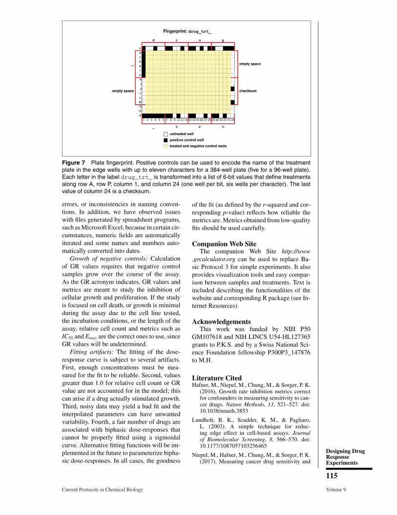
Figure 7 Plate fingerprint. Positive controls can be used to encode the name of the treatmentplate in the edge wells with up to eleven characters for a 384-well plate (five for a 96-well plate).Each letter in the label drug_trt_ is transformed into a list of 6-bit values that define treatmentsalong row A, row P, column 1, and column 24 (one well per bit, six wells per character). The lastvalue of column 24 is a checksum.

errors, or inconsistencies in naming conven-tions. In addition, we have observed issueswith files generated by spreadsheet programs,such as Microsoft Excel, because in certain cir-cumstances, numeric fields are automaticallyiterated and some names and numbers auto-matically converted into dates.

Growth of negative controls: Calculationof GR values requires that negative controlsamples grow over the course of the assay.As the GR acronym indicates, GR values andmetrics are meant to study the inhibition ofcellular growth and proliferation. If the studyis focused on cell death, or growth is minimalduring the assay due to the cell line tested,the incubation conditions, or the length of theassay, relative cell count and metrics such asIC50 and Emax are the correct ones to use, sinceGR values will be undetermined.

Fitting artifacts: The fitting of the dose-response curve is subject to several artifacts.First, enough concentrations must be mea-sured for the fit to be reliable. Second, valuesgreater than 1.0 for relative cell count or GRvalue are not accounted for in the model; thiscan arise if a drug actually stimulated growth.Third, noisy data may yield a bad fit and theinterpolated parameters can have unwantedvariability. Fourth, a fair number of drugs areassociated with biphasic dose-responses thatcannot be properly fitted using a sigmoidalcurve. Alternative fitting functions will be im-plemented in the future to parameterize bipha-sic dose-responses. In all cases, the goodness

of the fit (as defined by the r-squared and cor-responding p-value) reflects how reliable themetrics are. Metrics obtained from low-qualityfits should be used carefully.

Companion Web SiteThe companion Web Site http://www

.grcalculator.org can be used to replace Ba-sic Protocol 3 for simple experiments. It alsoprovides visualization tools and easy compar-ison between samples and treatments. Text isincluded describing the functionalities of thewebsite and corresponding R package (see In-ternet Resources).

AcknowledgementsThis work was funded by NIH P50

GM107618 and NIH LINCS U54-HL127365grants to P.K.S. and by a Swiss National Sci-ence Foundation fellowship P300P3_147876to M.H.

Literature CitedHafner, M., Niepel, M., Chung, M., & Sorger, P. K.

(2016). Growth rate inhibition metrics correctfor confounders in measuring sensitivity to can-cer drugs. Nature Methods, 13, 521–527. doi:10.1038/nmeth.3853

Lundholt, B. K., Scudder, K. M., & Pagliaro,L. (2003). A simple technique for reduc-ing edge effect in cell-based assays. Journalof Biomolecular Screening, 8, 566–570. doi:10.1177/1087057103256465

Niepel, M., Hafner, M., Chung, M., & Sorger, P. K.(2017). Measuring cancer drug sensitivity and


115




http://dx.doi.org/10.1038/nmeth.3853

http://dx.doi.org/10.1177/1087057103256465

resistance in cultured cells. Current Protocolsin Chemical Biology, 9(2), 1–20.

Powell, S. G., Baker, K. R., & Lawson, B. (2008).A critical review of the literature on spreadsheeterrors. Decision Support Systems, 46, 128–138.doi: 10.1016/j.dss.2008.06.001

Saez-Rodriguez, J., Goldsipe, A., Muhlich, J., Alex-opoulos, L. G., Millard, B., Lauffenburger, D.A., & Sorger, P. K. (2008). Flexible informaticsfor linking experimental data to mathematicalmodels via DataRail. Bioinformatics, 24, 840–847. doi: 10.1093/bioinformatics/btn018

Stocker, G., Fischer, M., Rieder, D., Bindea, G.,Kainz, S., Oberstolz, M., . . . Trajanoski, Z.(2009). iLAP: A workflow-driven software forexperimental protocol development, data acqui-sition and analysis. BMC Bioinformatics, 10,390–401. doi: 10.1186/1471-2105-10-390

Wu, T., & Zhou, Y. (2014). An intelligent automa-tion platform for rapid bioprocess design. Jour-nal of Laboratory Automation, 19, 381–393. doi:10.1177/2211068213499756

Zeeberg, B. R., Riss, J., Kane, D. W., Bussey, K. J.,Uchio, E., Linehan, W. M., . . . Weinstein, J. N.(2004). Mistaken identifiers: Gene name errorscan be introduced inadvertently when using Ex-cel in bioinformatics. BMC Bioinformatics, 5,80. doi: 10.1186/1471-2105-5-80

Ziemann, M., Eren, Y., El-Osta, A., Zeeberg, B.,Riss, J., Kane, D., . . . Smedley, D. (2016).Gene name errors are widespread in the scien-tific literature. Genome Biology, 17, 177. doi:10.1186/s13059-016-1044-7

Key ReferencesHafner et al. (2016). See above.Paper describing the GR method.

Niepel et al. (2017). See above.This article in Current Protocols in Chemi-

cal Biology is a companion article to thepresent article, including more experimentaldetail.

Internet Resourceshttps://github.com/datarail/datarailGitHub repository with the scripts for the experi-

mental design and data handling

https://github.com/datarail/gr_metricsGitHub repository with the scripts for the evaluation

of the GR values and metrics.

http://www.GRcalculator.orgGRcalculator: An online tool for calculating, visu-

alizing, and mining drug response data designedby Clark, N. A., Hafner, M., Kouril, M., Williams,E. H., Muhlich, J. L., Niepel, M., Medvedovic, M.

http://www.labautopedia.org/mw/Helpful_Hints_to_Manage_Edge_Effect_of_Cultured_Cells_for_High_Throughput_Screening

Helpful hints to manage edge effect of cultured cellsfor high throughput screening. Corning Cell Cul-ture Application and Technical Notes, 7–8 (au-thor, Allison Tanner of Corning Life Sciences,2001).


Experiments

116


http://dx.doi.org/10.1016/j.dss.2008.06.001

http://dx.doi.org/10.1093/bioinformatics/btn018

http://dx.doi.org/10.1186/1471-2105-10-390

http://dx.doi.org/10.1177/2211068213499756

http://dx.doi.org/10.1186/1471-2105-5-80

http://dx.doi.org/10.1186/s13059-016-1044-7



http://www.GRcalculator.org




designing drug-response experiments and quantifying their...

Documents