design space exploration using heuristic algorithms
TRANSCRIPT
DESIGN SPACE EXPLORATION USING HEURISTIC ALGORITHMS
by
Monica JayasheelGowda
APPROVED BY SUPERVISORY COMMITTEE:
___________________________________________
Dr. Benjamin Carrion Schaefer, Chair
___________________________________________
Dr. William Swartz
___________________________________________
Dr. Yang Hu

Copyright 2018
Monica JayasheelGowda
All Rights Reserved

Dedicated to my parents, sister and teachers.
DESIGN SPACE EXPLORATION USING HEURISTIC ALGORITHMS
by
MONICA JAYASHEELGOWDA, BE
THESIS
Presented to the Faculty of
The University of Texas at Dallas
in Partial Fulfillment
of the Requirements
for the Degree of
MASTER OF SCIENCE IN
ELECTRICAL ENGINEERING
THE UNIVERSITY OF TEXAS AT DALLAS
AUGUST 2018

v
ACKNOWLEDGMENTS
I would like to thank my thesis advisor, Dr Benjamin Carrion Schafer, for his constant support,
help and faith in my research work. His dedication towards his research has always inspired me
and motivated me to do more in my research work. He has always guided me and helped me in
the right direction whenever I made mistakes in my work. He has always encouraged me to
learn more and I would like to appreciate his patience and enthusiasm in helping and guiding
students under him. Thank you Professor for you faith in me and my work.
I would also like thank Dr. William Swartz and Dr. Yang Hu for being a part of my committee
and reviewing my work. I would like to thank the Electrical Engineering Department and Design
Automation and Reconfigurable Computing Lab (DARC Lab) for creating an inspiring research
environment and providing me with the required resources. I would like to heartily thank all my
lab mates, Mahesh, Himanshu, Farah, Zi, Siyuan, Jianqi and Zhiqi for their support and help. I
would like thank the Office of Graduate Studies for reviewing my work and giving their
suggestions. My humble thanks to my parents who supported me throughout my studies and
encouraged me to pursue my dreams. I would lastly like to thank all my friends for their
encouragement.
MAY 2018
vi
DESIGN SPACE EXPLORATION USING HEURISTIC ALGORITHMS
Monica JayasheelGowda, MSEE
The University of Texas at Dallas, 2018
ABSTRACT
Supervising Professor: Benjamin Carrion Schafer, Chair
In the field of High Performance Computing, Field Programmable Gate Arrays are growing
exponentially. The use of the High Level Synthesis Tools has resulted in an increase in the
applications which are intensive in computation such as Cognitive Computing Artificial
Intelligence due to the ease of its usage. The advantage of the increasing level of abstraction in
hardware design is it provides various configurations which have unique properties like area,
power, performance which can be generated automatically with no need to write the input
descriptions again. All of this would not be possible with the traditional languages such as
Verilog or VHDL. This thesis mainly focuses on the above mentioned topic which helps in
finding the most optimum solutions for the Design Space Exploration with the implementation
of the two Heuristic Algorithms such as the Genetic Algorithm and the Simulated Annealing.
This work mainly focuses on the exploration of High level synthesis for the design space
exploration and its automation using Qt creator. The Heuristic Algorithms for the Design Space
Exploration was developed to obtain the optimum values of the area versus latency. This
optimum value is obtained by inserting and varying various attribute knobs like loop unrolling,
`vii
arrays etc. in the benchmarks. These attributes play a very important role in obtaining the
optimum values which can be controlled and tuned with the help of the knobs which generate
various configurations of the micro architecture. It is hence not a feasible option to perform a
brute search or an exhaustive search on these values due to the large design space and also
complex and large designs, as a result this gives rise to the need of heuristic algorithms. The
Genetic Algorithm and Simulated Annealing Algorithms are hence explored for each benchmark
to obtain an optimum solution if not the best possible solution for a given design space. The
comparison of these three types of searches is done using quality metrics like the Average
Distance to Reference Set (ADRS) and Dominance which shows that the Genetic Algorithm
gives us a better result in comparison to Simulated Annealing. The whole process is automated
using Qt Creator which generates a Graphical User Interface for the process of automation.
viii
TABLE OF CONTENTS
ACKNOWLEDGMENTS ..............................................................................................................v
ABSTRACT ................................................................................................................................... vi
LIST OF FIGURES ...................................................................................................................... xii
LIST OF TABLES ....................................................................................................................... xiii
CHAPTER 1 INTRODUCTION ...................................................................................................1
1.1 Introduction To Traditional VLSI Flow ....................................................................1
1.2 Traditional VLSI Flow ...............................................................................................1
1.3 Thesis Flow ................................................................................................................3
CHAPTER 2 HIGH LEVEL SYNTHESIS ...................................................................................5
2.1 Introduction .................................................................................................................5
2.2 Steps In HLS ...............................................................................................................6
2.3 Concepts In HLS ........................................................................................................7
2.4 Modelling And Compilation ......................................................................................8
2.5 Allocation .................................................................................................................10
2.6 Scheduling................................................................................................................10
2.7 Binding .....................................................................................................................15
2.8 Advantages Of HLS .................................................................................................18
2.9 Disadvantages Of HLS ............................................................................................19
CHAPTER 3 CYBERWORKBENCH ........................................................................................21
3.1 Commercial HLS Tools ...........................................................................................21
3.2 CyberWorkBench ....................................................................................................21
CHAPTER 4 ATTRIBUTES .......................................................................................................23
4.1 Rules For Description ..............................................................................................23
4.2 Attribute Placement .................................................................................................25
4.3 Attributes Specific To SystemC...............................................................................26
4.4 Numeric Expressions In Attributes ..........................................................................27
4.5 Macro Substitution For An Attribute .......................................................................28
ix
4.6 CWB Explorer Attribute Limitation ........................................................................29
CHAPTER 5 DESIGN SPACE EXPLORATION ......................................................................30
CHAPTER 6 ALGORITHMS .....................................................................................................32
6.1 Heuristic Algorithms ................................................................................................32
6.2 Genetic Algorithm ...................................................................................................32
6.2.1 Introduction .....................................................................................................32
6.2.2 Algorithm ........................................................................................................34
6.2.3 Advantages ......................................................................................................35
6.2.4 Genetic Operations On Attribute Pool ............................................................35
6.2.5 Application Of Genetic Algorithm On Our Experiments ...............................40
6.2.6 Algorithm Overview .......................................................................................41
6.2.7 Effect Of Alpha And Beta On DSE ................................................................43
6.3 Simulated Annealing ................................................................................................44
6.3.1 Why Simulated Annealing? ............................................................................44
6.3.2 Application Of Simulated Annealing In Our Experiments .............................46
6.3.3 Algorithm Overview .......................................................................................48
CHAPTER 7 AVERAGE DISTANCE TO REFFERENCE SET AND DOMINANCE ...........50
7.1 ADRS .......................................................................................................................50
7.2 Application Of ADRS On Our Results ....................................................................51
7.3 Dominance ...............................................................................................................54
7.4 Application Of Dominance On DSE........................................................................54
CHAPTER 8 QT GRAPHICAL USER INTERFACE ................................................................55
8.1 What Is Qt? ..............................................................................................................55
8.2 Software Architecture Of Qt ....................................................................................55
8.2.1 GUI Abstraction ..............................................................................................55
8.2.2 Slots And Signals ............................................................................................56
8.2.3 MOC ...............................................................................................................56
8.2.4 Qt Modules......................................................................................................56
8.3 Implementation Of Qt GUI For Our DSE................................................................57
CHAPTER 9 EXPERIMENTAL RESULTS ..............................................................................59
x
9.1 Overview Of Complete Procedure ...........................................................................60
9.2 Results Of Benchmarks............................................................................................62
9.2.1 Ave8 ................................................................................................................62
9.2.2 FIR ..................................................................................................................65
9.2.3 Snow3G...........................................................................................................67
9.2.4 Interpolation ....................................................................................................70
9.2.5 FFT ..................................................................................................................73
9.2.6 Kasumi ............................................................................................................75
9.3 Result Tabulation .....................................................................................................78
CHAPTER 10 CONCLUSION AND FUTURE WORK ............................................................80
10.1 Conclusion .............................................................................................................80
10.2 Future Work ..........................................................................................................80
REFERENCES ..............................................................................................................................81
BIOGRAPHICAL SKETCH .........................................................................................................84
CURRICULUM VITAE ................................................................................................................85
xi
LIST OF FIGURES
Figure 1.1 Traditional VLSI Flow ...................................................................................................2
Figure 1.2 Thesis Flow ....................................................................................................................4
Figure 2.1 Design Steps Of High Level Synthesis ..........................................................................8
Figure 2.2 ASAP Scheduling Example ..........................................................................................11
Figure 2.3 Example Of ALAP Scheduling ....................................................................................13
Figure 2.4 Mix ALAP And ASAP Scheduling Example ...............................................................14
Figure 2.5 Example To Illustrate Basic Idea Of Binding ..............................................................15
Figure 2.6 High Level Synthesis Main Steps.................................................................................17
Figure 5.1 Design Space Exploration For High Level Synthesis ..................................................31
Figure 6.1 A Graphical Representation Of Roulette Wheel Selection [14] ..................................36
Figure 6.2 Crossover Of Parents (One-Point Crossover) [14] .......................................................37
Figure 6.3 Crossover Of Parent Attributes ....................................................................................39
Figure 6.4 Genetic Algorithm Overview .......................................................................................40
Figure 6.5 Report Generated After Genetic Algorithm’s Execution .............................................41
Figure 6.6 Flow Of Genetic Algorithm .........................................................................................42
Figure 6.7 Genetic Algorithm For DSE .........................................................................................43
Figure 6.8 Effect Of Alpha And Beta On DSE ..............................................................................44
Figure 6.9 Report Of Simulated Annealing Algorithm’s Application ...........................................47
Figure 6.10 Flow Of Simulated Annealing Algorithm ..................................................................48
Figure 6.11 Simulated Annealing On DSE ....................................................................................49
Figure 7.1 Average Distance To Reference Set .............................................................................50
Figure 7.2 Variable Instantiation ...................................................................................................52
Figure 7.3 Calculation Of Individual Distances ............................................................................52
Figure 7.4 Calculation Of Dist (A1, B1)........................................................................................53
Figure 7.5 ADRS Implementation .................................................................................................53
Figure 7.6 Dominance Graph .........................................................................................................54
Figure 7.7 Dominance Calculation ................................................................................................54
Figure 8.1 Overview Of GUI .........................................................................................................57
xii
Figure 9.1 Experimental Setup ......................................................................................................59
Figure 9.2 Library File For FFT. ...................................................................................................60
Figure 9.3 Selection Of Algorithm ................................................................................................61
Figure 9.4 Command To Run On Console ....................................................................................61
Figure 9.5 Results From .CSV File ................................................................................................61
Figure 9.6 DSE Plot OF The .CSV File Generated .......................................................................62
Figure 9.7 Quality Metrics. ............................................................................................................62
Figure 9.8 Ave8 Genetic Algorithm ..............................................................................................63
Figure 9.9 Ave8 Simulated Annealing...........................................................................................64
Figure 9.10 FIR Genetic Algorithm ...............................................................................................66
Figure 9.11 FIR Simulated Annealing ...........................................................................................67
Figure 9.12 Snow3G Genetic Algorithm .......................................................................................68
Figure 9.13 Snow3G Simulated Annealing ...................................................................................69
Figure 9.14 Interpolation Genetic Algorithm ................................................................................71
Figure 9.15 Interpolation Simulated Annealing.............................................................................72
Figure 9.16 FFT Genetic Algorithm ..............................................................................................73
Figure 9.17 FFT Simulated Annealing ..........................................................................................75
Figure 9.18 Kasumi Genetic Algorithm.........................................................................................76
Figure 9.19 Kasumi Simulated Annealing .....................................................................................77
xiii
LIST OF TABLES
Table 3.1 Features Of BDL [17] ....................................................................................................22
Table 4.1 Attributes List ...............................................................................................................27
Table 6.1 Naming Convention In Genetic Algorithm ...................................................................33
Table 8.1 Qt Essentials ..................................................................................................................56
Table 9.1 Genetic Algorithm Results.............................................................................................78
Table 9.2 Simulated Annealing Results .........................................................................................79
1
CHAPTER 1
INTRODUCTION
1.1 Introduction To VLSI Design Flow:
The term VLSI stands for Very large scale integrated circuit. It is a combination of thousands of
transistors which are combined together to create an IC (integrated circuit). VLSI was developed
in 1970’s during the development of communication and semiconductor technologies, prior to the
VLSI technology the Integrated circuits performance factors where limited. The semiconductor
industry has seen an exponential growth over the decades because of the advanced system design
and the integration technologies which are implemented in a large scale. After the emergence of
VLSI technology there has been an increase in the applications of an Integrated circuit in
telecommunications, high performance computing, video and image processing etc. which was as
predicted by Moore’s law which explains that the number of transistors in an Integrated circuit
doubles every two years[23].
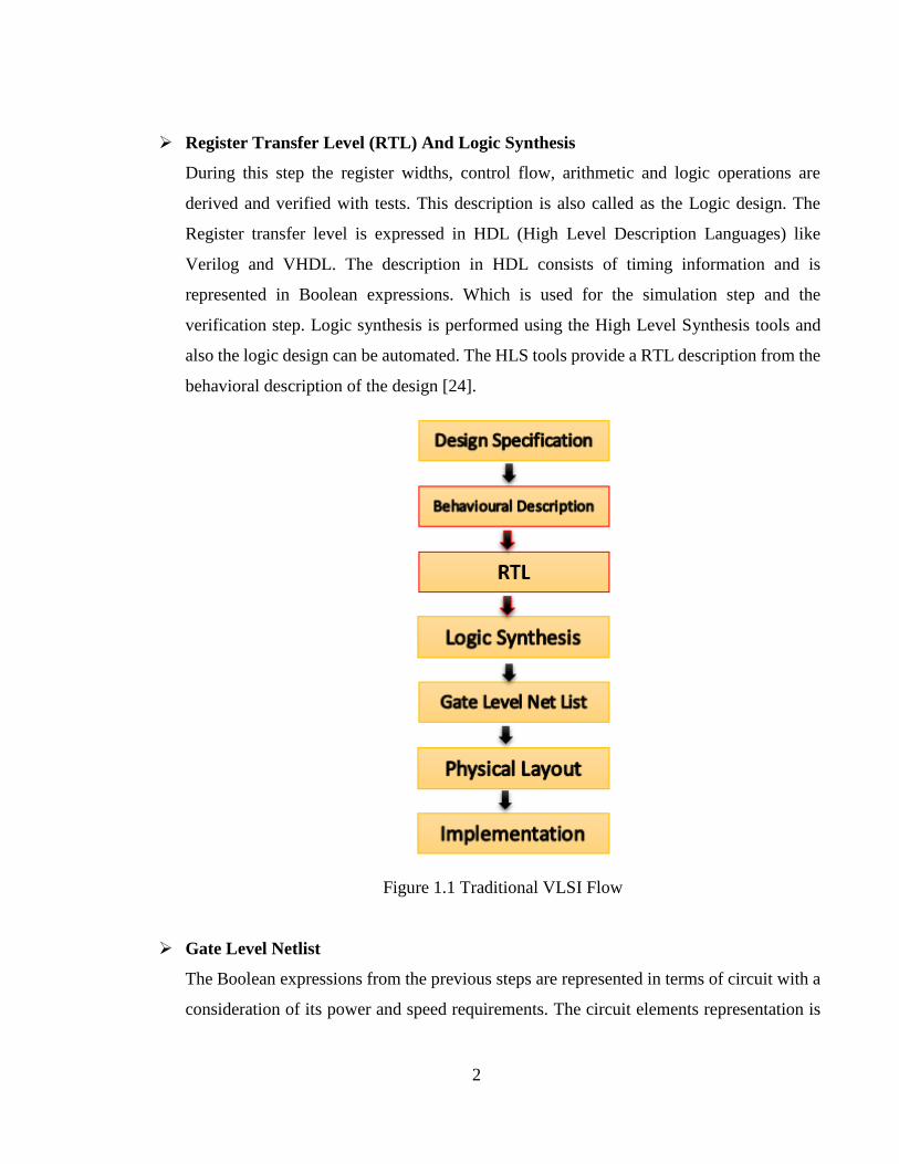
1.2 Traditional VLSI Design Flow
The traditional flow of a VLSI design circuit is as shown in the figure 1.1.
System Specification
This is the initial step for a design process where the system’s design specifications are
specified in the form of high level representation. It specification consists of factors like
the functionality, performance, fabrication technology, physical dimensions etc.
Behavioral Description
In the behavioral description step the functional unit and the required interconnections are
recognized. The importance of this description is to describe the behavior with respect to
the output, input and the timing requirements. This results in a functional design with a
timing diagram. After this step we obtain the data which helps us to reduce the complexity
and improve the design process.
2
Register Transfer Level (RTL) And Logic Synthesis
During this step the register widths, control flow, arithmetic and logic operations are
derived and verified with tests. This description is also called as the Logic design. The
Register transfer level is expressed in HDL (High Level Description Languages) like
Verilog and VHDL. The description in HDL consists of timing information and is
represented in Boolean expressions. Which is used for the simulation step and the
verification step. Logic synthesis is performed using the High Level Synthesis tools and
also the logic design can be automated. The HLS tools provide a RTL description from the
behavioral description of the design [24].
Figure 1.1 Traditional VLSI Flow
Gate Level Netlist
The Boolean expressions from the previous steps are represented in terms of circuit with a
consideration of its power and speed requirements. The circuit elements representation is
3
done with the help of a netlist. A netlist is a representation of macros, cells, transistors and
gates and also the interconnections which lie in between the elements mentioned. With the
help of logic synthesis tools we can generate a netlist from the RTL description.
Physical Layout
A physical layout is generated by converting the circuit represented with a help of the
netlist which implements the logical function of the component from the netlist. Logic
Synthesis tools can be used to partially or completely automate and generate the layout
from the generated netlist.
Implementation
Once the layout has been generated it is verified and tested followed by the fabrication
process where the design is implemented. Further the final chip generated from the
fabrication process goes into packaging testing and debugging.
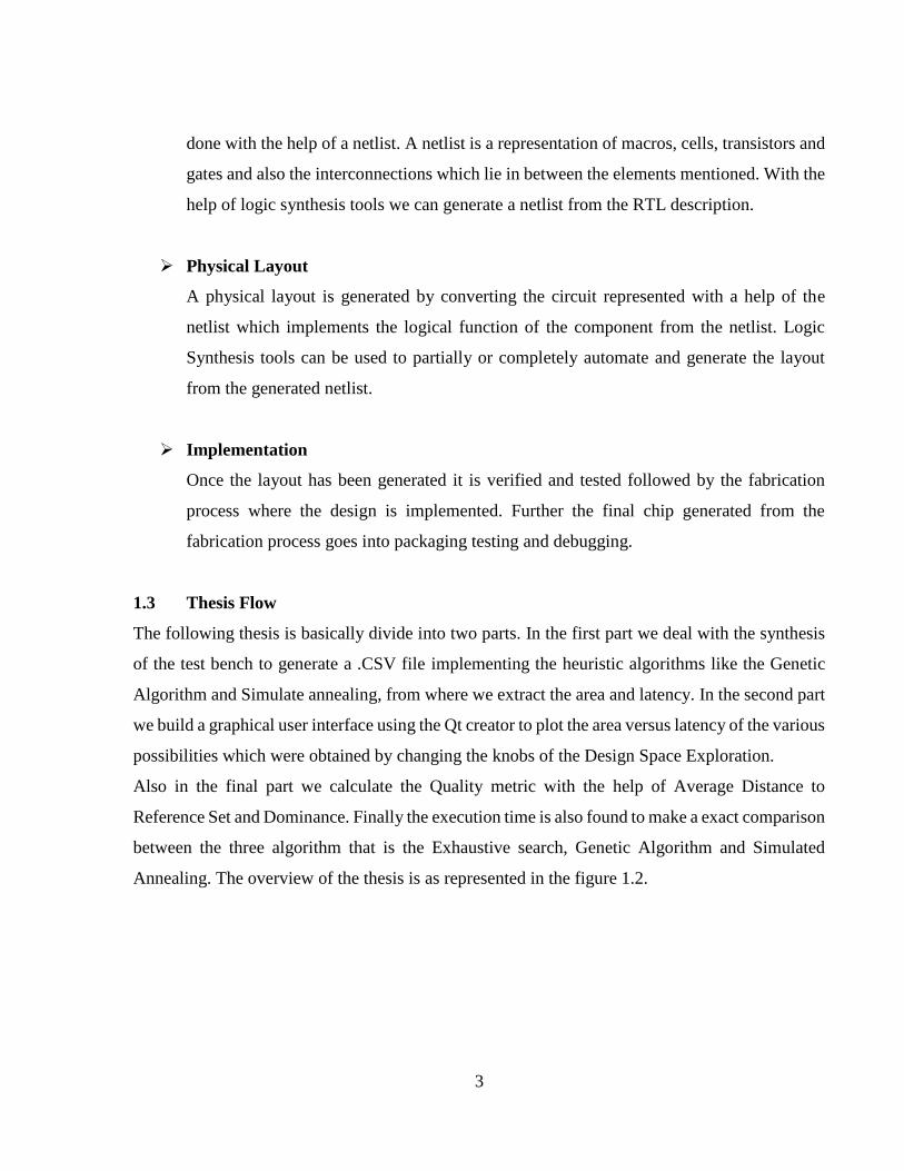
1.3 Thesis Flow
The following thesis is basically divide into two parts. In the first part we deal with the synthesis
of the test bench to generate a .CSV file implementing the heuristic algorithms like the Genetic
Algorithm and Simulate annealing, from where we extract the area and latency. In the second part
we build a graphical user interface using the Qt creator to plot the area versus latency of the various
possibilities which were obtained by changing the knobs of the Design Space Exploration.
Also in the final part we calculate the Quality metric with the help of Average Distance to
Reference Set and Dominance. Finally the execution time is also found to make a exact comparison
between the three algorithm that is the Exhaustive search, Genetic Algorithm and Simulated
Annealing. The overview of the thesis is as represented in the figure 1.2.
4
Figure 1.2. Thesis Flow
5
CHAPTER 2
HIGH LEVEL SYNTHESIS
2.1 Introduction
In this era of leading edge silicon innovation and technology the exponential complexities and
intricacy in their applications has compelled us to approach these design techniques into a more
efficient way of abstractions of higher levels. The main principle factor for this evolvement of the
process of design techniques (process) is the increased levels of abstraction and also the
automation process for synthesis and verification process and allows an efficient way of design
space exploration.
In the arena of software, let us say we have a sequence of binary digits which once upon a time
was the only way to program and code the computer. During 1950’s an assembler or assembly
level language was presented. Further to improve the proficiency and productiveness of a software
based High Level Languages was developed which had its own compilation methods or
techniques. These High Level Languages are independent of platform, they have rules, and syntax
it also hides the computer architecture details making it tractable and portable. Today we use
assembly level programing for a few cases like optimization of a program and to make it more
compact. We can say that the effort towards finding a better result using High Level Languages
and its respective compilers is happening irrespective of the complexity of the systems architecture
or its software application; because imagine to code for a complex application using assembly
language isn’t it time consuming plus we would need a very highly skilled professional to write a
very efficient code in assembly language.
The domain of hardware has its own design procedures and language specifications have grown
along the same lines. Until 1960’s, the design and layout of IC was done by hand and in the late
1970’s cycle based simulation was made commercial.
In the decade from 1980 to 1990 there was a new life for this field and a lot of new technologies
and innovations were made such as techniques like schematic circuit, place and route, verification
and STA (static timing analysis). A huge range of adaptation in these tools for simulation was
provided because of the Hardware Description languages like Verilog and VHDL. These Hardware
6
Description languages can be used to define the functionalities as an input to these synthesizing
tools.
In 1990’s the High level synthesis’s first version was made available in the market. During the
same time there was a huge growing interest in the research of design of hardware and software
hat is the co-design of software-hardware which took into account the co-simulation, partitioning
and interface, synthesis, estimation, exploration and communication this resulted in the invention
of design of the IP cores and design of platform based systems.
The year 2000’s gave a diversion towards ESL (electronics system level) which supports
verification and synthesis of complicated system on chips (SoCs). This initiated use of language’s
like SystemC, SpecC, Transaction level modelling and system Verilog these also increased the
complexities of the system giving rise to a need to provide an improved differential variant of the
chip making it interdependent leading the spotlight towards the hardware-software efficiency,
susceptibility, productivity and its ability to be reused. All of these factors have made it evident to
find a more design efficient ESL. The High level synthesis flow reduces the time required for
verification and other aspects like the analysis off power usage.
2.2 Steps In High Level Synthesis:
Increasing the abstraction level of a hardware design is required to explore its system level
architectural pronouncement like configuration of its memory, the ways power is managed, its
verification and synthesis procedures and also its design of software-hardware techniques. The
High level Synthesis has a feature of reusability of a similar or the same specifications at high
level, aimed at giving place for a huge variety of ASIC and FPGA design constraints.
Let us get into the steps in the process of the High level synthesis. Firstly the designer starts the
implementation of the processor’s by providing the application’s specification like its required
coprocessor or its dedicated hardware unit like the arbiter, interrupt controllers, interface and
special function unit along with the capture of the functionality of the high level descriptions using
High level languages. So basically this step is associated with writing the specifications of the
function of the unit which involves the concurrent consumption of the input and computes this
data with no delay and simultaneously gives an output.
7
In this level of abstraction data types (like int, char, and double) and variables (like arrays and
structures) are not related to either the embedded software or design of the hardware. During the
generation of an improvised architecture for hardware beginning from the specifications of its bit
accuracy it is important to generate an acceptable accuracy for computation for the
implementation. A conversion of integer and floating point data type into a data type which is bit
accurate for a specific length in a realistic hardware would be needed in order to achieve this.
The High level Synthesis tools convert partially timed or untimed specifications to an
implementation which is timed fully. They also generate an architecture which can be implement
its specifications efficiently which is generated semi automatically or automatically. This
generated architecture is illustrated or described at RTL level and consists of the controllers and
data path (like buses, multiplexers, registers and functional units) following the design constraints
and the given specifications.
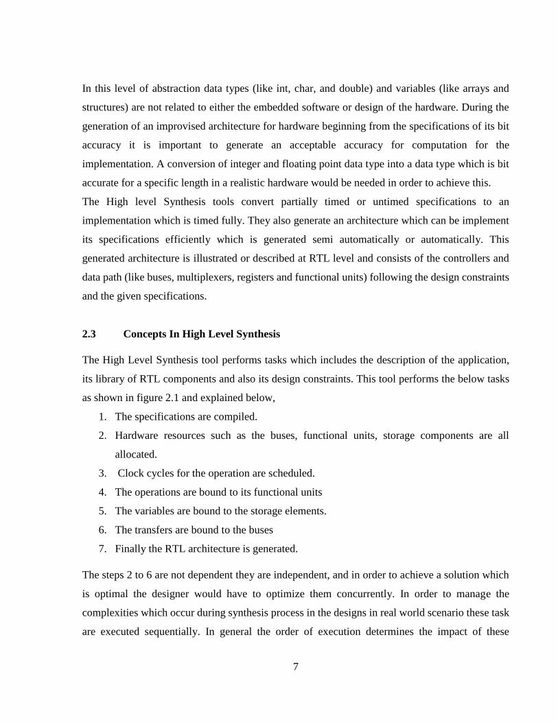
2.3 Concepts In High Level Synthesis
The High Level Synthesis tool performs tasks which includes the description of the application,
its library of RTL components and also its design constraints. This tool performs the below tasks
as shown in figure 2.1 and explained below,
1. The specifications are compiled.
2. Hardware resources such as the buses, functional units, storage components are all
allocated.
3. Clock cycles for the operation are scheduled.
4. The operations are bound to its functional units
5. The variables are bound to the storage elements.
6. The transfers are bound to the buses
7. Finally the RTL architecture is generated.
The steps 2 to 6 are not dependent they are independent, and in order to achieve a solution which
is optimal the designer would have to optimize them concurrently. In order to manage the
complexities which occur during synthesis process in the designs in real world scenario these task
are executed sequentially. In general the order of execution determines the impact of these
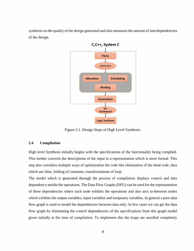
8
synthesis on the quality of the design generated and also measures the amount of interdependencies
of the design.
Figure 2.1. Design Steps of High Level Synthesis.
2.4 Compilation
High level Synthesis initially begins with the specifications of the functionality being complied.
This further converts the descriptions of the input to a representation which is more formal. This
step also considers multiple ways of optimization the code like elimination of the dead code, data
which are false, folding of constants, transformations of loop.
The model which is generated through the process of compilation displays control and data
dependency amidst the operations. The Data Flow Graphs (DFG) can be used for the representation
of these dependencies where each node exhibits the operations and also arcs in-between nodes
which exhibits the output variables, input variables and temporary variables. In general a pure data
flow graph is used to model the dependencies between data only. In few cases we can get the data
flow graph by eliminating the control dependencies of the specifications from this graph model
given initially at the time of compilation. To implement this the loops are unrolled completely
9
through the conversation of code blocks which are not iterative and the conditional assignment is
determined through the creation of values which are multiplexed. The data flow graphs shows the
possible inherent parallelism for the given specification. Moreover these transformations results
in a need for a reasonable amount memory at the time of the synthesis process. But one drawback
is that these form of representation is not supported by loops that have iteration counts which are
unbounded and non-static control statements like goto. Due to all these factors it results in a
limitation in the use of the pure data flow graph representation in some applications. Hence to
overcome this limitation the data flow graph is extended to by the addition of control dependency
which forms a control and data flow graph (CDFG).
In a control and data flow graph the edges will portray its control flow. Nodes of a control and data
flow graph which referred are also as basic blocks which is nothing but a sequence of straight line
like statements with no internal entrance or branches or point of exit. Here their edges could be a
condition for the representation of the constructs like if and switch. This type of data graph consist
of data dependencies within the basic block of the control data flow graph which would take into
account the control flow within these basic blocks.
Control and Data flow graphs are much expensive in comparison to data flow graphs which can
be due to the fact that these CDFG’s can also be used to illustrate loops which would have iterations
that are unbounded. It is observed that the parallelism is more accurate only when used in basic
blocks and some more analysis and transformations may be necessary to unveil the parallelism
which might be existing within the basic blocks. Loop tiling, loop pipelining, loop merging, loop
unrolling are a few examples of such transformations. Such methods, expose the parallelism in-
between loop iterations and the loop which are very helpful in optimization of the number and size
of the memory accesses and also throughput or the latency. Such transformation could be user
driven or automatically be realized. It is also possible to add the control and dependencies to
control data graphs as represented in the HTG (Hierarchical task graph).
Below are the three main steps of High Level Synthesis:
1. Allocation
2. Scheduling
3. Binding
10
2.5 Allocation
The allocation step it is used define or instantiate the number of hardware resources like the
connectivity or storage components, functional units and the types of hardware resources required
for the design constraints. Based on the tool used for high level synthesis few components can be
included during binding and scheduling the task. Let us consider an example like the components
used for connectivity like the point to point connection or buses which can be included after or
prior to the scheduling and binding of the tasks. The RTL component library is the repository for
these components. At least a minimum of one component needs to select for every operation in
the model specifications. The repository of this library has to take into account the characteristics
of the components like the delay, power and area and also the metrics which has to be used by
different synthesis functions or tasks.
2.6 Scheduling
In general the given specification model contains operations which have to be scheduled in terms
of cycles. For all the individual operation like a=b op c, the term b and c should be read from their
respective sources like their functional unit or storage components which will perform the op
operation and their result is stored in variable a and got to its storage unit or functional unit. Based
on these functional units on which the functionality is mapped, scheduling of the operations are
done either to schedule them to a number of cycles or done in one cycle. The output of these
operations can be sent as an input to another operation that is the operations have an option to be
chained. They can also be parallelized if there are no data dependencies and they have the required
resources at that point of time.
Scheduling assigns automatically the control procedures to the design constraints. The scheduling
uses algorithms to execute its functionality it can be divided into two parts they are exact and
heuristic which are used to solve the problems faced due to scheduling such as resource constraints,
time constraints, time and resource constraints, and unconstrained. In Exact algorithms for
scheduling such as the Linear Programing, gives an optimal schedule but consumes more time to
process (high process time).
11
In order to take care of the high time consumption for execution, various algorithms have been
created which takes decisions as to which point in the local analysis gives the best step. Hence
they might skip an optimum solution, but in practice they also produce quick results which are
almost very close to optimum solutions. These algorithms are known as the heuristic algorithms.
Few examples of such algorithms are ALAP As Late As Possible, ASAP As Soon As Possible,
FDS Forced Directed Scheduling, LS List Scheduling. Few of these algorithms can either be time
constrained scheduling like the ALSP, ASAP and FDS or be resource constrained scheduling.
Let have a small introduction about these algorithms.
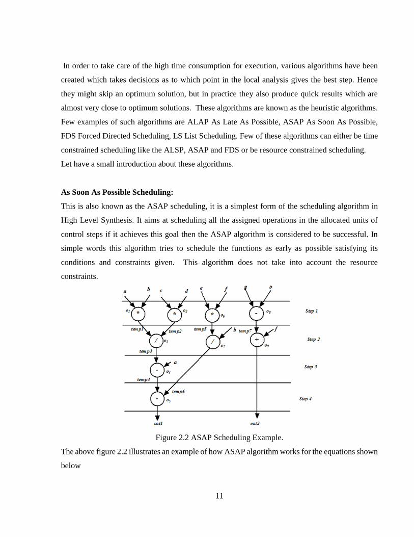
As Soon As Possible Scheduling:
This is also known as the ASAP scheduling, it is a simplest form of the scheduling algorithm in
High Level Synthesis. It aims at scheduling all the assigned operations in the allocated units of
control steps if it achieves this goal then the ASAP algorithm is considered to be successful. In
simple words this algorithm tries to schedule the functions as early as possible satisfying its
conditions and constraints given. This algorithm does not take into account the resource
constraints.
Figure 2.2 ASAP Scheduling Example.
The above figure 2.2 illustrates an example of how ASAP algorithm works for the equations shown
below
12
out1 = ((a*b)/(c*d))-a-(e*f)/b) (1)
out2 = (g-b) + f (2)
and M = 4
where M = maximum number of steps for scheduling process.
Here from the graph above we observe that the functions o-1, 2, 6, 8 depend on their input values
and they have no direct antecedent. Whereas the function o3 has two antecedents o2, o1; using
these two predecessors we can calculate the control step assignment for the function o3 as follows,
CS of O3 = max (CS of o2, CS of o3)+1 = 2 (3)
Where CS = control step.
On the similar lines we can calculate the step assignment for each operation.
It takes 4 steps for ASAP to be completed in this example with a usage of the following resources:
1. First Step uses three multipliers, one subtractor (3 Multipliers, 1 Subtractor).
2. Second Step uses two dividers and one adder (2 Divider, 1 Adder).
3. Third Step no new resources are used, here the subtractor from the first step is used.
4. Fourth Step no new resources are used, here the subtractor from the first step is used.
ALAP:
This scheduling algorithm is also called as the As Late As Possible scheduling process. This falls
in the same line of ASAP but it first finds the maximum number of control steps instead of directly
scheduling the operations like in ASAP scheduling. After this step this algorithm takes one
operation at a time and schedules it to the latest possible step only if its further operations are
scheduled in latter steps. Even ALAP does not take into account resource constraints like ASAP.
The above figure 2.3 illustrates an example of how ALAP algorithm works for the equations
shown below
out1 = ((a*b)/(c*d))-a-(e*f)/b) (4)
out2 = (g-b) + f (5)
and M = 4
where M = maximum number of steps for scheduling process.
13
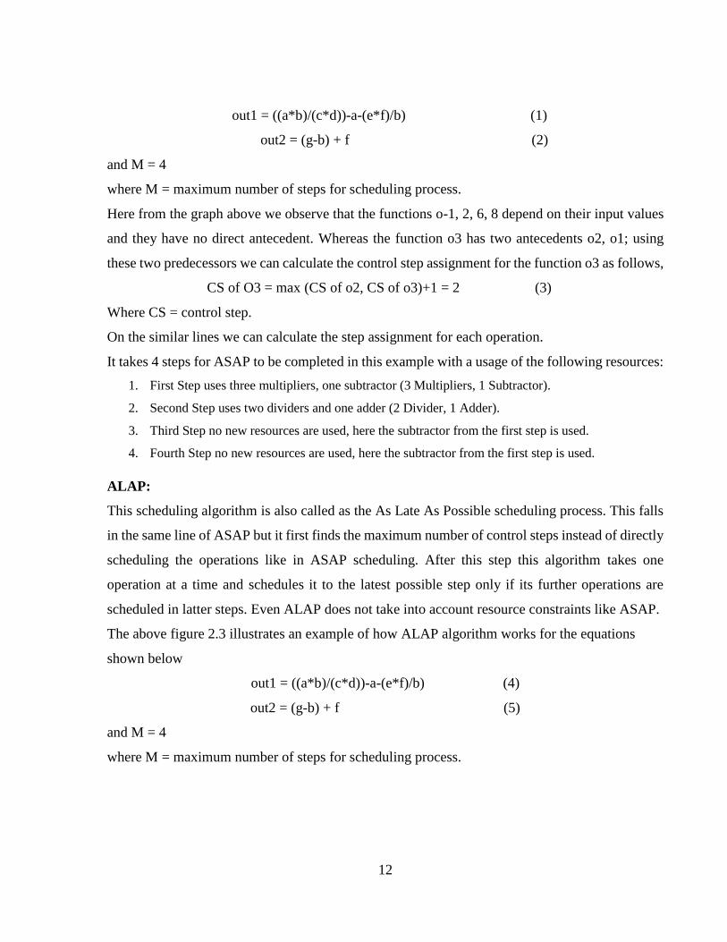
Figure 2.3. Example Of ALAP Scheduling
Here from the figure 2.3 as shown above we observe that the functions o5 and o9 have no
ascendants hence they would give an output value, hence they have a step number of 4 (M=4). We
observe that 05 has a direct ascendant o4 hence we can calculate the assignment of control steps
as follows
CS of o5 = CS of o5 – 1 = 3. (6)
On the same lines we can calculate the assignment of all possible operations.
This example completes its ALAP scheduling in its first control step and is thus successful. The
resource usage are
1. First Step: Uses two multipliers (2 Multipliers).
2. Second Step: Uses one dividers and one multiplier from previous step.
3. Third Step: Uses two subtracts and divider from the previous step.
4. Fourth Step: One adder and a subtractor from previous step.
If we compare the examples of ASAP and ALAP we can see that
One multiplier is saved due to the delay in o6 from the first step to the second step.
One divider is saved due to the delay in o7 from second step to the third step.
14
But there is an increase of one subtractor through the delay in o8 from first step to the third
step.
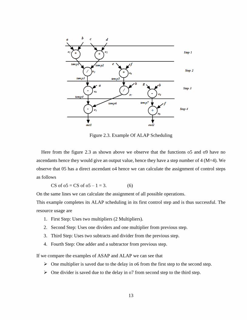
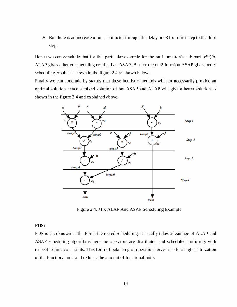
Hence we can conclude that for this particular example for the out1 function’s sub part (e*f)/b,
ALAP gives a better scheduling results than ASAP. But for the out2 function ASAP gives better
scheduling results as shown in the figure 2.4 as shown below.
Finally we can conclude by stating that these heuristic methods will not necessarily provide an
optimal solution hence a mixed solution of bot ASAP and ALAP will give a better solution as
shown in the figure 2.4 and explained above.
Figure 2.4. Mix ALAP And ASAP Scheduling Example
FDS:
FDS is also known as the Forced Directed Scheduling, it usually takes advantage of ALAP and
ASAP scheduling algorithms here the operators are distributed and scheduled uniformly with
respect to time constraints. This form of balancing of operations gives rise to a higher utilization
of the functional unit and reduces the amount of functional units.
15
This type of scheduling algorithm initially searches the ALAP and ASAP scheduling for all the
given operations. If the number of control steps are same then no action is taken and the operations
are not rescheduled. If the ALAP and ASAP schedule of these operators are different and has a
flexible range then all such operations will be listed. After this step it will schedule all operations
so as to find a minimum total count of operators. In order to achieve this functionality this
scheduling process considers one type of operation at a time.
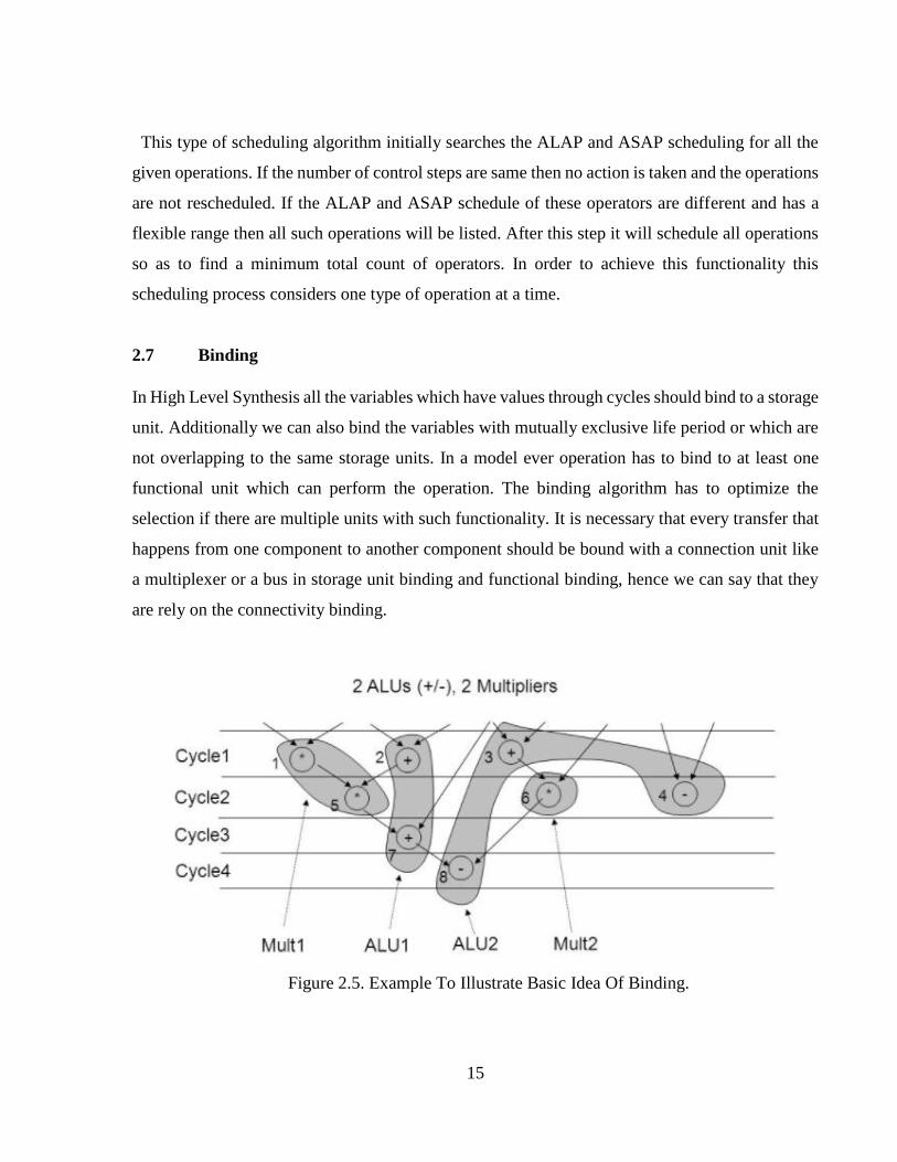
2.7 Binding
In High Level Synthesis all the variables which have values through cycles should bind to a storage
unit. Additionally we can also bind the variables with mutually exclusive life period or which are
not overlapping to the same storage units. In a model ever operation has to bind to at least one
functional unit which can perform the operation. The binding algorithm has to optimize the
selection if there are multiple units with such functionality. It is necessary that every transfer that
happens from one component to another component should be bound with a connection unit like
a multiplexer or a bus in storage unit binding and functional binding, hence we can say that they
are rely on the connectivity binding.
Figure 2.5. Example To Illustrate Basic Idea Of Binding.
16
The basic idea of binding in the above figure 2.5 is to map operations with the given resource
constraints in such a way that the same resources are not used in the same cycle of operations.
So we can say that Binding is associated with a resource that has each operation of the similar type
and finds the implemented area. Sharing is done to bind the resource to two or more non-concurrent
operations.
In a Resource dominant circuit the area and latency is found as shown below,
The area is found by the binding process.
AREA = ∑area of resources bound in the given operation.
This is found during Scheduling process.
Latency = Start time of sink – Start time of source.
In a Non Resource dominant circuit,
The Area is affected by the steering logic, wiring, control and the registers used.
The Cycle time is affected by the wiring, control and the steering logic.
In an ideal situation the HLS finds the area and latency as soon as possible in order to find an
optimized design in the future HLS steps. Another way to optimize is to give a detailed architecture
at the time of allocation process such that these maps of architecture can be further used during
the process of scheduling and binding.
Some of the Binding algorithms are,
Binding through clique partitioning
Binding through Left Edge Algorithm
Binding through Iterative Refinement
These were the three main steps of the High Level Synthesis i.e the Allocation, scheduling and
Binding. These three processes can be sequentially or simultaneously performed based on the
algorithm which is being used, but to keep a note about these three processes are interrelated.
When performed simultaneously they may be very complex for real world applications and
examples. In general the order of execution is determined based on the objective of the tools being
used and also the design constraints of the model used.
17
Let us consider the scenario where the allocation process is performed in the beginning if the
scheduling process is attempting to reduce the latency or improve the throughput with a constraint
of resources. Allocation is arbitrated when scheduling is making an attempt to reduce the area with
a constraint in timing.
When a designer requires to define the architecture of the data path or to improvise the application
with the use of an FPGA which has a restricted resource availability an approach of resource
constraint is used. On the other side a time constraint method is used when we need to minimize
the area of the circuit when the throughput requirement of the application is fulfilled like in cases
of telecommunication and multimedia examples.
The problems dealing with resource constraints can be resolved using an approach which involves
time constrained method of solution and when there is a timing constrained problem it can be
resolved using a resource constrained approach. In such situations the designer will simmer down
the timing constraint till the point where an acceptable circuit area is generated. The constraints
such as resource, throughput, area and latency are quite well known, but in the recent research and
work they consider factors like the memory bandwidth, clock period, memory mapping and the
consumption of power which complicate the solution of synthesis problems.
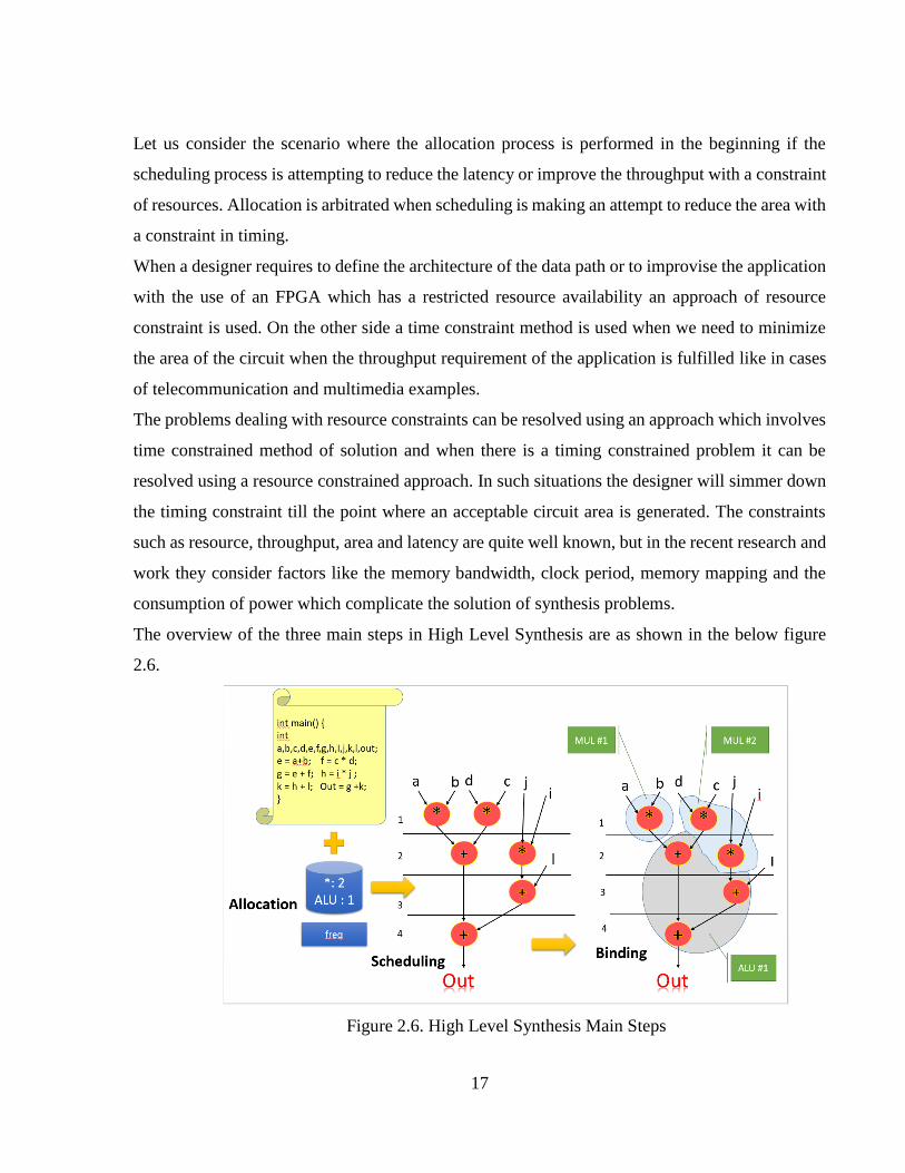
The overview of the three main steps in High Level Synthesis are as shown in the below figure
2.6.
Figure 2.6. High Level Synthesis Main Steps
18
2.8 Advantages Of High Level Synthesis
1. A code can be transported easily from an implementation in software to that of an
implementation in hardware with the help of HLS.
2. There are various versions of compilers that can operate with standard C code and compile
C code to a RTL and the tool further synthesizes it into an FPGA. Usually just the software
code compilation is enough in the CPU based processors as the software algorithms are
used for implementing this on the processor. It is required to reconstruct the algorithm
based on the hardware requirements and the resources available in the hardware. So
instead of manually converting C to RTL the High Level Synthesis can be used to
reconstruct onto a high level source and this would be much easier and the resulting errors
would be reduced.
3. The implicit representation of the control path is one of the key advantage of HLLs.
The High Level Synthesis tools extracts and builds its control path based on the studies
made on the loop structure, branch structures or other possible structures of the algorithms.
In case of complex algorithms the control path’s designing may endeavour more work
than designing a data path.
4. In environments which have coprocessors the computations are used by both the CPU and
the High Level Synthesis enabling the source code which could be compiled as software
or hardware allowing the various modules to be swapped from hardware to software and
vice versa which helps to find an optimum mixture of the two.
5. For a code which is structured well the latest High Level Synthesis tools generates an
efficient design equivalent to that of an RTL with respect to both processing speed and the
resources used.
Synthesis tools usually exploit parallelization in the following three methods:
1. The data dependencies are found through the analysis of the dataflow. Through this we can
conjecture the sequence of processing and pipeline to meet time-constraints if required.
2. Through the loop analysis which requires quite some processing with restricted
dependency in between the iteration. This permits to infer an architecture which is
19
pipelined and where a successive iteration could start without any dependency on the
previous iterations completion.
3. Through loop unrolling hardware blocks which have multiple parallelism have been
constructed to start the iterations which can be parallelised.
2.9 Disadvantages Of High Level Synthesis
1. The hardware board can be a bloated design if the code is not structured properly for the
HLS tool to perform synthesis on it. That is we must write the algorithm is a particular way
such that the tool will be able to identify and perform parallelize it. So the unstructured
code has to be restructured properly.
2. The main factor is that the designs based on FPGA are not software they are hardware
designs. No matter if the synthesis language is HLS or RTL it will always describe design
of the hardware to be built and is not an executable instruction set of statements.
3. When we use HLS for the purpose of synthesis it is very important to remember that we
should not slip into a mind-set of a software coder. Hence the hardware description
languages when treated like a software it has high chances to leading to confusions or may
result in a non- efficient usage of the hardware.
4. The representation of the algorithms for software is quite stable, whereas for realizations
in hardware it’s still in infant stages despite of the ongoing research.
5. Pointer based algorithms are not well synthesized in HLS because pointers sometimes
make it difficult for the high level synthesis tools to find data dependencies. Also pointers
poses in two difficulties when implementing the FPGA .One is that the FPGA has a
distributed memory on-chip which have their own address space and are small and
independent blocks. Other is that majority of the variables are stored in registers.
6. Another software technique called Recursion is not well translated in hardware. This
happens because on FPGA implements a function as a hardware block with multiplexing
the hardware for every call. But the hardware has no stack and the variables declared locally
are stored in registers which use the mutual for each invocation this results in reuse of the
20
registers. Hence recursive algorithms are reconstructed and uses its identical iteration block
instead.
7. It is difficult to design systems which operate concurrently because it needs
synchronization although High Level Synthesis takes care of synchronization and
parallelization efficiently for complex models with multiple parallel processors it is not
that dependable.
8. The RTL which is generated by the High Level Synthesis tool is not easily readable and
difficult to modify the code.
21
CHAPTER 3
CYBERWORKBENCH
3.1 Tools Used For Performing High Level Synthesis
Some of the tools used for performing HLS are:
1. Cadence CtoSilicon: This tools uses C, C++ and SystemC languages.
2. Xilinx Vivado HLS: C, C++ and SystemC are the languages used.
3. Mentor Graphics CatapaultC : This uses languages like C++ and SystemC
4. NEC Cyberworkbench: This tool uses C and SystemC languages. This is our tool of interest
and we will look into the details of this tool.
3.2 CWB
Cyberworkbench is basically a High level synthesis and verification tool which is used to
synthesize designs for applications for ASIC and FPGA’s.
This tool converts a behavioral description in systemC or Behavioral Description language into an
optimized and synthesized form of a RTL code like VHDL and Verilog for FPGAs and ASICS’s.
The cyberworkbench mainly has the following five tools they are:
1. A tool to convert the BDL to an internal format like the .IFF file.
2. A tool to perform Behavioural Synthesis.
3. A tool to RTL description in VHDL and Verilog
4. Other sub tools
5. Finally has a Graphical User Interface to manage all the tools.
The languages used in CWB are
SystemC: It is an antecedent of Accellera Systems Initiative as defined by OSCI. It is a
C++ language’s class of library which makes the description of hardware or system model
easier in the High Level Language. Its library is approved from IEEE1666 standards.
22
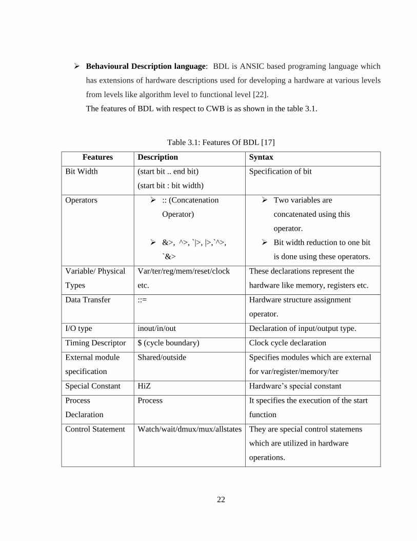
Behavioural Description language: BDL is ANSIC based programing language which
has extensions of hardware descriptions used for developing a hardware at various levels
from levels like algorithm level to functional level [22].
The features of BDL with respect to CWB is as shown in the table 3.1.
Table 3.1: Features Of BDL [17]
Features Description Syntax
Bit Width (start bit .. end bit)
(start bit : bit width)
Specification of bit
Operators :: (Concatenation
Operator)
&>, ^>, `|>, |>,`^>,
`&>
Two variables are
concatenated using this
operator.
Bit width reduction to one bit
is done using these operators.
Variable/ Physical
Types
Var/ter/reg/mem/reset/clock
etc.
These declarations represent the
hardware like memory, registers etc.
Data Transfer ::= Hardware structure assignment
operator.
I/O type inout/in/out Declaration of input/output type.
Timing Descriptor $ (cycle boundary) Clock cycle declaration
External module
specification
Shared/outside Specifies modules which are external
for var/register/memory/ter
Special Constant HiZ Hardware’s special constant
Process
Declaration
Process It specifies the execution of the start
function
Control Statement Watch/wait/dmux/mux/allstates They are special control statemens
which are utilized in hardware
operations.
23
CHAPTER 4
ATTRIBUTES
In CyberWorkBench we have a set of attribute pallet from where we choose the most suitable
attribute for a given piece of code. So let us see as to what attribute means and learn its structure
how to use it and the syntax so that we can understand its application in our research.
So basically attributes are a set of comments that begin with the key word or a string of character
like “Cyber” or “CwbExplorer” which signifies an attribute. The implementation of these attributes
is to specify the method used by the Behavioral Synthesis system’s method of synthesis.
Syntax for ATTRIBUTES: The syntax to declare an attribute is as shown below
/* Cyber attribute name = attribute value */
/* Cyber attribute name */
//Cyber attribute name = attribute value
//Cyber attribute name
4.1 Rules For Description
1. Type “Cyber” at the beginning of the comment.
The word “Cyber” is not case sensitive.
Tabs, spaces and line feed characters defined in between “//” or “/* */”.
After the word “Cyber” it should contain a tab or a space.
In the comment if “Cyber” is not present then it is considered to be a normal
comment and not an attribute.
2. We can describe multiple attributes if they are separated with commas between them.
/* Cyber name1 = val1, name2 = val2*/
/* Cyber name3 = val3 */
3. We can describe a line feed character as shown below,
/* Cyber attri_name1 = val1,
Attri_name2 = val2 */
24
4. We need to declare the attribute for a statement just before the statement.
An attribute assigned for a function definition
/* Cyber func = inline */
Var (0”8) func ( var(0:8) i )
{
}
Assigning an attribute to a for statement
/* Cyber unroll_times =all */
for ( i = 0; i<=5; i ++)
{
}
5. Attribute should be declared immediately after a declaration :
An attribute is attached to a the variable g.
int g /* Cyber share_name = REG01 */;
An attribute is attached to a variable h.
out reg (0:8) h /* Cyber valid_sig = b_i */ = 3;
An attribute is attached to a function declaration.
Var (0:8) funcA(var (0:8) b ) /* Cyber func = inline */;
6. A block can be declared using an attribute immediately before it.
/* Cyber scheduling_block */
{
a = b;
c = d;
}
7. We can vary the effect of an attribute through the substitution of a macro.
#define ARRAY_en RAM
int n[8] /* Cyber array = ARRAY_en */;
25
4.2 Attribute Placement:
Let’s see the places where we can add attributes:
Process Function:
The attributes for a process function has to be defined before the function definition as
shown below:
SC_MOODULE(Module name)
{
:
/* Cyber name = value */
Void entry()
{
:
}
:
};
This how we add an attribute to the process function.
Hierarchical description of the Top Module:
In case of a hierarchical description we can define multiple processes. It is done as shown
below:
SC_MODULE (module name)
{
/* Cyber name = value */
SC_CTOR (module name)
{
:
}
}
Function and Member Function:
26
An attribute can be added to before the definition start of a member function when
specified. The usage of the attribute in a function is as shown below:
/* Cyber name = value */
int foo (int arg)
{
:
Return result;
}
Variables:
If a local or member variable is specified, an attribute is added after its definition.
The way to specify an attribute to a variable is as shown below:
int var /* Cyber name = value */
Statements:
For statements the attributes are specified before the statement definition as shown in the
below example:
/* Cyber name = value */
for (int i=0; i<16; i++)
{
:
}
Operator:
In case of an operator the attribute is specified after the operator is defined as shown below:
i = i + /*Cyber name = value */ j;
4.3 Attributes Specific To SystemC:
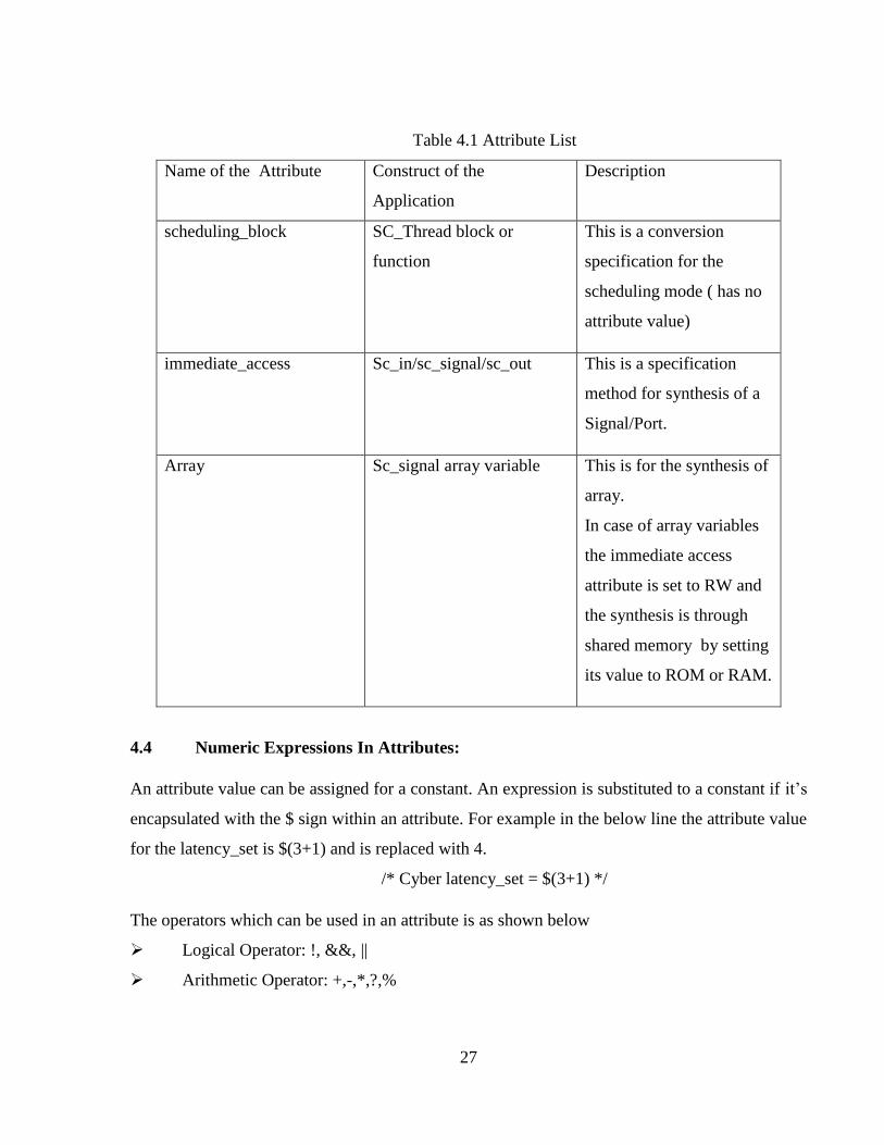
The attributes which are specific to SystemC are as shown in the below table 4.1.
27
Table 4.1 Attribute List
Name of the Attribute Construct of the
Application
Description
scheduling_block SC_Thread block or
function
This is a conversion
specification for the
scheduling mode ( has no
attribute value)
immediate_access Sc_in/sc_signal/sc_out This is a specification
method for synthesis of a
Signal/Port.
Array Sc_signal array variable This is for the synthesis of
array.
In case of array variables
the immediate access
attribute is set to RW and
the synthesis is through
shared memory by setting
its value to ROM or RAM.
4.4 Numeric Expressions In Attributes:
An attribute value can be assigned for a constant. An expression is substituted to a constant if it’s
encapsulated with the $ sign within an attribute. For example in the below line the attribute value
for the latency_set is $(3+1) and is replaced with 4.
/* Cyber latency_set = $(3+1) */
The operators which can be used in an attribute is as shown below
Logical Operator: !, &&, ||
Arithmetic Operator: +,-,*,?,%

28
Ternary Oprator: (?:)
Comaprison Operator : <, <=, >, >=, !=, ==
Bit Operator: <<, >>, &, |, ^, ~
4.5 Macro Substitution For An Attribute:
We can substitute an attribute in the comment with a macro pre-processor. We can also control
the synthesized circuit using this.
For example let us consider the attribute unroll_times which is used for a loop and we r replacing
it the with UNROLL_TYPE macro. Usually we expect the latency for a circuit with a large area
to be small. If we replace 0 with ALL then the loop is unrolled completely and this results in an
increased area and results in a high speed synthesizable circuit.
#define UNROLL_TYPE 0
// Cyber unroll_times = UNROLL_TYPE
for (char i=0; i<32; i++)
{
x=i;
wait();
}
Another example of marco substitution for an attribute where an array n1 and n2 is implemented
through memory or register
#define ATTR_GROUP1 Cyber
#define ATTR_GROUP2
char n1[256] /* ATTR_GROUP1 array = RAM, sig2mu=memA */
/* ATTR_GROUP2 array=REG */;
char n2[256] /* ATTR_GROUP1 array = RAM, sig2mu=memA */
/* ATTR_GROUP2 array=REG */;
29
4.6 CWB Explorer Attribute Limitations:
An attribute which are defined in Cyber can also be defined in a similar way in CWB Explorer but
some cannot be specified.
Stall_control
Immediate_access
Scheduling_block which is appended to the function SC_THREAD.
The attributes which are mentioned above are some exceptions which can’t be declared in CWB
Explorer. They throw an error if used.
30
CHAPTER 5
DESIGN SPACE EXPLORATION
The Design Space Exploration (DSE) is a bustle of exploration into finding alternatives for design
of a system before its implementation. DSE refers to systematic analysis and pruning of unwanted
design points based on parameters of interest [20] The Design Space Exploration has various
applications such as analysis of trade off, rapid prototyping and finding an optimum design for a
given or the required parameter.
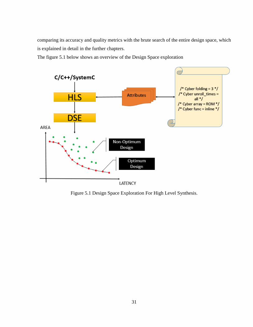
The advantage of this design is that the High Level Synthesis gives us permission to modify the
Micro-Architecture of the design and there is no need to make any changes to its behavioral
descriptions. The above procedure is done through setting various synthesis options such as the
Pragmas and the Attributes like loop unroll factor, array etc. which is explained in detail in the
previous topic.
These attributes affects the performance, memory access and the resource utilization directly by
varying its Micro-Architecture. Hence various possibilities of such combinations generates a huge
set of designs which have various configurations and they further have different performance
characteristics based on these individual attributes. The prediction of the performance of such
attributes is quite difficult since we cannot predict the exact combination of these attributes which
would provide an optimal solution with best required results since their interaction with each other
cannot be foreseen. For instance let us consider that the number of computational units are
increased this means that the performance should also increase due to the parallel running
processes. Whereas this need not be correct always since there are chances that the requirement of
high bandwidth of the memory can degrade the performance due to reasons like stalling Hence it
is required to test these attributes on many testing designs to get an optimum design. Also due to
its extremely huge search space it is impractical to prototype the whole search space solution due
to the constraints in the time. This forces us to use heuristic methods which are faster approach in
searching a good solution in the given time constraints from the design space. In our experiments
we are using the Genetic Algorithm and the Simulated Annealing Algorithms to achieve this and
31
comparing its accuracy and quality metrics with the brute search of the entire design space, which
is explained in detail in the further chapters.
The figure 5.1 below shows an overview of the Design Space exploration
Figure 5.1 Design Space Exploration For High Level Synthesis.
32
CHAPTER 6
ALGORITHMS
As explained in Chapter 5 we require various heuristic algorithms to obtain a good set off results
from the design space for a given time frame since its practically not optimum to perform a brute
search for all the designs to obtain an optimum solution. In order to achieve this we perform various
Heuristic Algorithms on the attributes defined for the design and obtain the results based on these
algorithms.
6.1 Heuristic Algorithms:
The algorithms which find a solution from all the possibilities but not does not assure the best
solution for a given set of data are called as Heuristic Algorithms. Hence they are just an
approximation and not the exact solution. The Heuristic Algorithm finds the closest solution to the
best solution easily and fast. There are times when the heuristic algorithms could find the best
solution and are accurate. They are used when there is no need to find the optimum or the best
solution but the approximate solution is sufficient and in cases were the best solutions are
expensive in terms of its computation. Below are a few types of Heuristic Algorithms:
Swarm Intelligence
Simulated Annealing
Support Vector Machines
Genetic Algorithm
Artificial Neural Network
6.2 Genetic Algorithm
6.2.1 Introduction
Finding a solution to a mathematical problem of the real world would include many stages such
as mathematical modelling, idealizations or simplification solutions to the real time problem and
finally concluding with an answer.
33
Since around 60 years, a transformation of ideals has occurred-in a sense, the converse has come
into trend. Even before the advent of mathematical modelling, the world succeeded in the
discovery of methods and operations. Explicitly, there is a vast variety of extremely refined
techniques and theories that have invariably mesmerized the researchers due to their excellence.
Emulating such principles mathematically and use them as a solution for wider class of issues has
proven to be useful in numerous fields of study i.e. a probabilistic optimization method which is
based on the principles of evolution.
In a nutshell, here are three examples:
Artificial Neural Networks(ANN):
Neuron’s basic models and interactions used for numerous applications such as machine
learning, function approximation and pattern recognition.
Fuzzy control :
A mathematical modelling system based on a set of control rules and fuzzy logic which
helps analyse analytical models and processes.
Simulated Annealing:
Robust probabilistic optimization method mimicking the solidification of a crystal under
slowly decreasing temperature; applicable to a wide class of problems [14].
Genetic Algorithm:
It is a replica of evolution. Mostly, genetic algorithms are just methods of probabilistic
optimization built on the fundamentals of evolution.
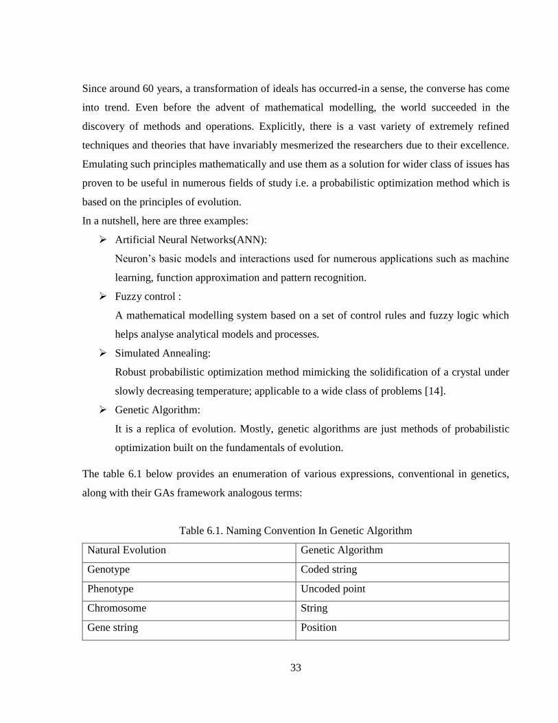
The table 6.1 below provides an enumeration of various expressions, conventional in genetics,
along with their GAs framework analogous terms:
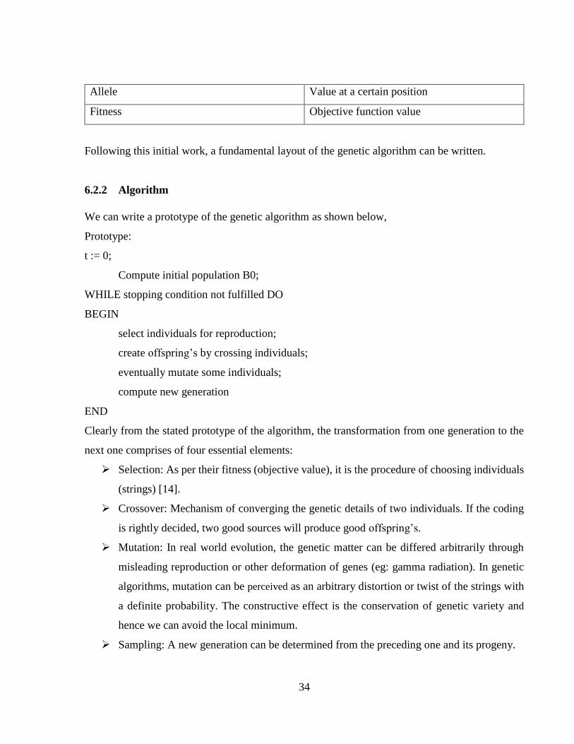
Table 6.1. Naming Convention In Genetic Algorithm
Natural Evolution Genetic Algorithm
Genotype Coded string
Phenotype Uncoded point
Chromosome String
Gene string Position
34
Allele Value at a certain position
Fitness Objective function value
Following this initial work, a fundamental layout of the genetic algorithm can be written.
6.2.2 Algorithm
We can write a prototype of the genetic algorithm as shown below,
Prototype:
t := 0;
Compute initial population B0;
WHILE stopping condition not fulfilled DO
BEGIN
select individuals for reproduction;
create offspring’s by crossing individuals;
eventually mutate some individuals;
compute new generation
END
Clearly from the stated prototype of the algorithm, the transformation from one generation to the
next one comprises of four essential elements:
Selection: As per their fitness (objective value), it is the procedure of choosing individuals
(strings) [14].
Crossover: Mechanism of converging the genetic details of two individuals. If the coding
is rightly decided, two good sources will produce good offspring’s.
Mutation: In real world evolution, the genetic matter can be differed arbitrarily through
misleading reproduction or other deformation of genes (eg: gamma radiation). In genetic
algorithms, mutation can be perceived as an arbitrary distortion or twist of the strings with
a definite probability. The constructive effect is the conservation of genetic variety and
hence we can avoid the local minimum.
Sampling: A new generation can be determined from the preceding one and its progeny.
35
6.2.3 Advantages:
In contrast with the optimization techniques conventionally used such as the Newton or gradient
descent methods, we can observe the following benefits:
1. GAs influences coded versions of the problem specifications instead of the specifications
themselves i.e. the search space S instead of X itself [14].
2. Although nearly all traditional techniques explore from a sole point, GAs always works on
the whole populace of points (strings).This presents a good deal to the robustness of genetic
algorithms. It enhances the possibility of attaining the global optimum and vice versa,
decreases the likelihood of getting trapped in a regional static point.
3. Usual genetic algorithms do not utilize any additional data related to the value of the
objective function like the derivatives. Hence, it can be implemented on any kind of issues
like the discrete or continuous optimization issues.
4. GAs use the probabilistic change promoters while the traditional techniques. For
continuous optimization apply deterministic transition operators [14].More precisely, the
method for a new generation that is determined from the primitive one will have few erratic
components.
6.2.4 Genetic Operations On Attribute Pool
1. Selection of the Attribute form the Attribute Pool:
Selection of the parent attributes from the attribute pool is a deterministic operation, but in most
of the executions it possesses few random parts. It is the element that models the algorithm to the
answer by choosing attributes with favourable high fitness over low-fitted ones.
Here, the fitness is directly proportional to the chances of choosing a particular individual. It can
be considered as an random trial where
P [bj,t is selected] = f(bj,t)
∑ f(bk,t)mk=1
(6.2.1)
The above stated formula will be clear only if the value of fitness are positive.
36
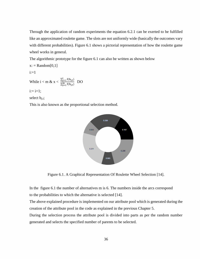
Through the application of random experiments the equation 6.2.1 can be exerted to be fulfilled
like an approximated roulette game. The slots are not uniformly wide (basically the outcomes vary
with different probabilities). Figure 6.1 shows a pictorial representation of how the roulette game
wheel works in general.
The algorithmic prototype for the figure 6.1 can also be written as shown below
x: = Random[0,1]
i:=1
While i < m & x < ∑ f(bj,t)i
j=1
∑ f(bj,t)mj=1
DO
i:= i+1;
select bj,t;
This is also known as the proportional selection method.
Figure 6.1. A Graphical Representation Of Roulette Wheel Selection [14].
In the figure 6.1 the number of alternatives m is 6. The numbers inside the arcs correspond
to the probabilities to which the alternative is selected [14].
The above explained procedure is implemented on our attribute pool which is generated during the
creation of the attribute pool in the code as explained in the previous Chapter 5.
During the selection process the attribute pool is divided into parts as per the random number
generated and selects the specified number of parents to be selected.
37
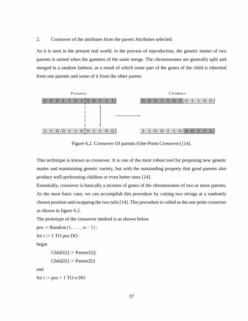
2. Crossover of the attributes from the parent Attributes selected:
As it is seen in the present real world, in the process of reproduction, the genetic matter of two
parents is united when the gametes of the same merge. The chromosomes are generally split and
merged in a random fashion, as a result of which some part of the genes of the child is inherited
from one parents and some of it from the other parent.
Figure 6.2. Crossover Of parents (One-Point Crossover) [14].
This technique is known as crossover. It is one of the most robust tool for proposing new genetic
matter and maintaining genetic variety, but with the outstanding property that good parents also
produce well-performing children or even better ones [14].
Essentially, crossover is basically a mixture of genes of the chromosomes of two or more parents.
As the most basic case, we can accomplish this procedure by cutting two strings at a randomly
chosen position and swapping the two tails [14]. This procedure is called as the one point crossover
as shown in figure 6.2.
The prototype of the crossover method is as shown below
pos := Random{1, . . . , n − 1};
for i := 1 TO pos DO
begin
Child1[i] := Parent1[i];
Child2[i] := Parent2[i]
end
for i := pos + 1 TO n DO
38
begin
Child1[i] := Parent2[i];
Child2[i] := Parent1[i]
end
One-point crossover is an easy and recurrently used technique for GAs that works on binary
strings. Other crossover techniques can be useful for other issues and different coding.
N-point crossover: N breaking points are chosen in a vague/random manner, instead of just
one. Swap occurs for every second portion. Among this type of class, the two point
crossover is very important.
Segmented crossover: Here, the number of breaking points can vary and is quite similar to
N-point crossover.
Uniform crossover: For every position, it is randomly decided if those positions are
swapped or not.
Shuffle crossover: A randomly chosen permutation is applied to the parents, then the N-
point crossover is applied to the parents that are rearranged, finally, the children that are
shuffled are altered back with inverse permutation.
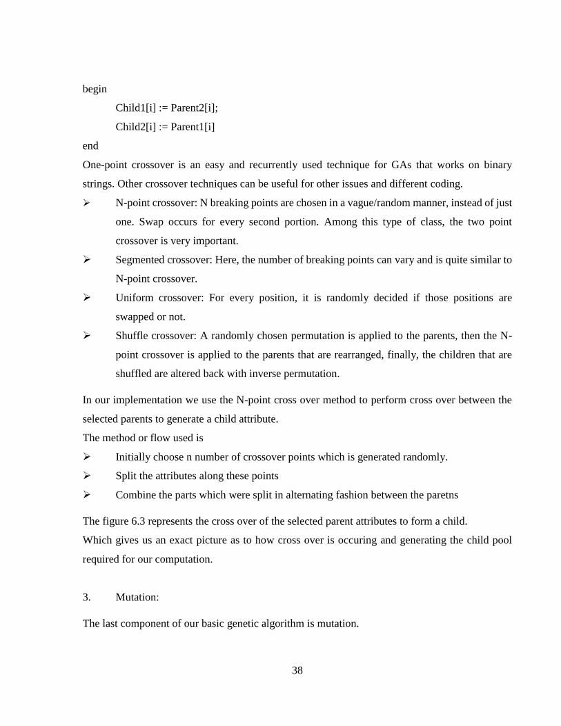
In our implementation we use the N-point cross over method to perform cross over between the
selected parents to generate a child attribute.
The method or flow used is
Initially choose n number of crossover points which is generated randomly.
Split the attributes along these points
Combine the parts which were split in alternating fashion between the paretns
The figure 6.3 represents the cross over of the selected parent attributes to form a child.
Which gives us an exact picture as to how cross over is occuring and generating the child pool
required for our computation.
3. Mutation:
The last component of our basic genetic algorithm is mutation.
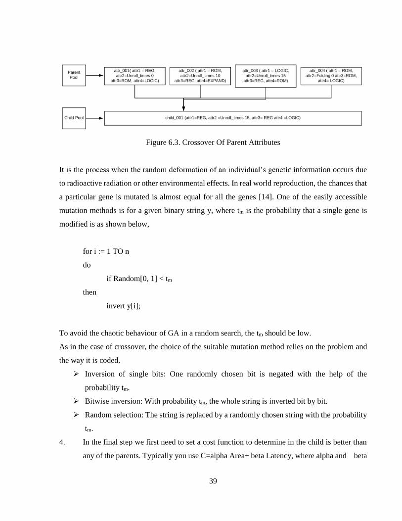
39
Figure 6.3. Crossover Of Parent Attributes
It is the process when the random deformation of an individual’s genetic information occurs due
to radioactive radiation or other environmental effects. In real world reproduction, the chances that
a particular gene is mutated is almost equal for all the genes [14]. One of the easily accessible
mutation methods is for a given binary string y, where tm is the probability that a single gene is
modified is as shown below,
for i := 1 TO n
do
if Random[0, 1] < tm
then
invert y[i];
To avoid the chaotic behaviour of GA in a random search, the tm should be low.
As in the case of crossover, the choice of the suitable mutation method relies on the problem and
the way it is coded.
Inversion of single bits: One randomly chosen bit is negated with the help of the
probability tm.
Bitwise inversion: With probability tm, the whole string is inverted bit by bit.
Random selection: The string is replaced by a randomly chosen string with the probability
tm.
4. In the final step we first need to set a cost function to determine in the child is better than
any of the parents. Typically you use C=alpha Area+ beta Latency, where alpha and beta
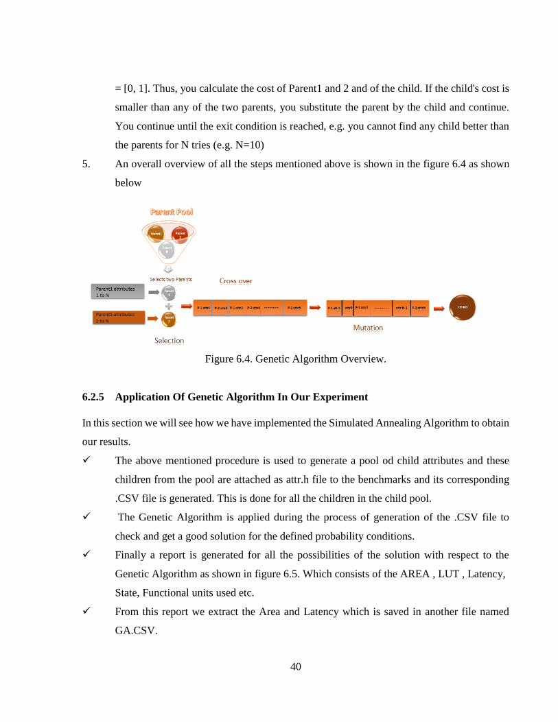
40
= [0, 1]. Thus, you calculate the cost of Parent1 and 2 and of the child. If the child's cost is
smaller than any of the two parents, you substitute the parent by the child and continue.
You continue until the exit condition is reached, e.g. you cannot find any child better than
the parents for N tries (e.g. N=10)
5. An overall overview of all the steps mentioned above is shown in the figure 6.4 as shown
below
Figure 6.4. Genetic Algorithm Overview.
6.2.5 Application Of Genetic Algorithm In Our Experiment
In this section we will see how we have implemented the Simulated Annealing Algorithm to obtain
our results.
The above mentioned procedure is used to generate a pool od child attributes and these
children from the pool are attached as attr.h file to the benchmarks and its corresponding
.CSV file is generated. This is done for all the children in the child pool.
The Genetic Algorithm is applied during the process of generation of the .CSV file to
check and get a good solution for the defined probability conditions.
Finally a report is generated for all the possibilities of the solution with respect to the
Genetic Algorithm as shown in figure 6.5. Which consists of the AREA , LUT , Latency,
State, Functional units used etc.
From this report we extract the Area and Latency which is saved in another file named
GA.CSV.
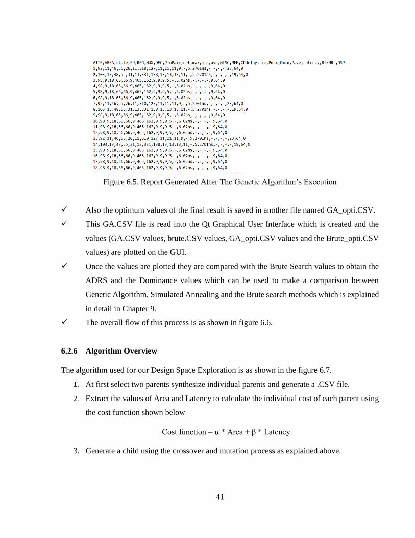
41
Figure 6.5. Report Generated After The Genetic Algorithm’s Execution
Also the optimum values of the final result is saved in another file named GA_opti.CSV.
This GA.CSV file is read into the Qt Graphical User Interface which is created and the
values (GA.CSV values, brute.CSV values, GA_opti.CSV values and the Brute_opti.CSV
values) are plotted on the GUI.
Once the values are plotted they are compared with the Brute Search values to obtain the
ADRS and the Dominance values which can be used to make a comparison between
Genetic Algorithm, Simulated Annealing and the Brute search methods which is explained
in detail in Chapter 9.
The overall flow of this process is as shown in figure 6.6.
6.2.6 Algorithm Overview
The algorithm used for our Design Space Exploration is as shown in the figure 6.7.
1. At first select two parents synthesize individual parents and generate a .CSV file.
2. Extract the values of Area and Latency to calculate the individual cost of each parent using
the cost function shown below
Cost function = α * Area + β * Latency
3. Generate a child using the crossover and mutation process as explained above.
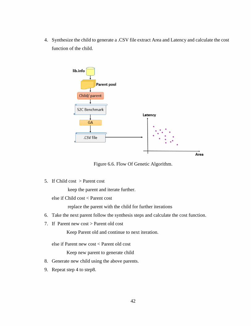
42
4. Synthesize the child to generate a .CSV file extract Area and Latency and calculate the cost
function of the child.
Figure 6.6. Flow Of Genetic Algorithm.
5. If Child cost > Parent cost
keep the parent and iterate further.
else if Child cost < Parent cost
replace the parent with the child for further iterations
6. Take the next parent follow the synthesis steps and calculate the cost function.
7. If Parent new cost > Parent old cost
Keep Parent old and continue to next iteration.
else if Parent new cost < Parent old cost
Keep new parent to generate child
8. Generate new child using the above parents.
9. Repeat step 4 to step8.
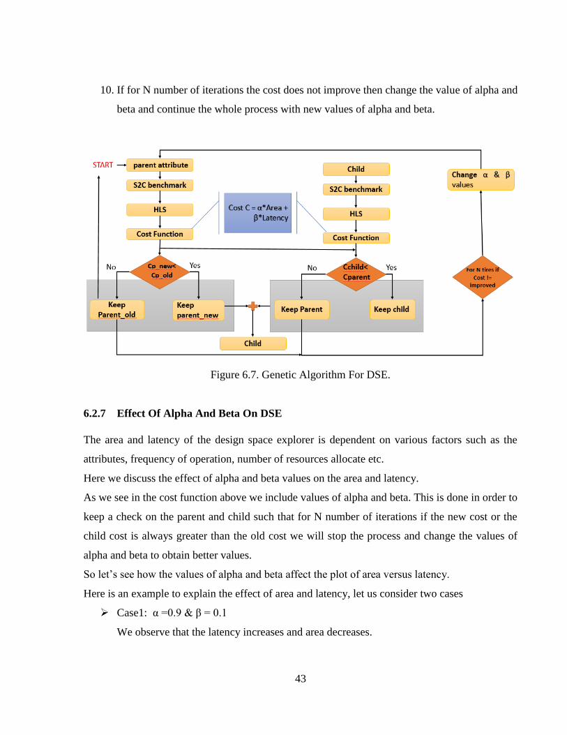
43
10. If for N number of iterations the cost does not improve then change the value of alpha and
beta and continue the whole process with new values of alpha and beta.
Figure 6.7. Genetic Algorithm For DSE.
6.2.7 Effect Of Alpha And Beta On DSE
The area and latency of the design space explorer is dependent on various factors such as the
attributes, frequency of operation, number of resources allocate etc.
Here we discuss the effect of alpha and beta values on the area and latency.
As we see in the cost function above we include values of alpha and beta. This is done in order to
keep a check on the parent and child such that for N number of iterations if the new cost or the
child cost is always greater than the old cost we will stop the process and change the values of
alpha and beta to obtain better values.
So let’s see how the values of alpha and beta affect the plot of area versus latency.
Here is an example to explain the effect of area and latency, let us consider two cases
Case1: α =0.9 & β = 0.1
We observe that the latency increases and area decreases.
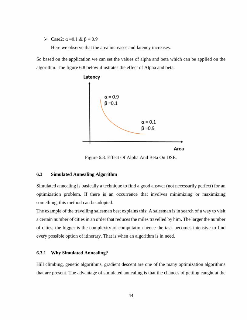
44
Case2: α =0.1 & β = 0.9
Here we observe that the area increases and latency increases.
So based on the application we can set the values of alpha and beta which can be applied on the
algorithm. The figure 6.8 below illustrates the effect of Alpha and beta.
Figure 6.8. Effect Of Alpha And Beta On DSE.
6.3 Simulated Annealing Algorithm
Simulated annealing is basically a technique to find a good answer (not necessarily perfect) for an
optimization problem. If there is an occurrence that involves minimizing or maximizing
something, this method can be adopted.
The example of the travelling salesman best explains this: A salesman is in search of a way to visit
a certain number of cities in an order that reduces the miles travelled by him. The larger the number
of cities, the bigger is the complexity of computation hence the task becomes intensive to find
every possible option of itinerary. That is when an algorithm is in need.
6.3.1 Why Simulated Annealing?
Hill climbing, genetic algorithms, gradient descent are one of the many optimization algorithms
that are present. The advantage of simulated annealing is that the chances of getting caught at the
45
local maxima is avoided, hence the solutions which are better than the ones nearby are found but
they need not be the best of all the solutions.
1. Optimization problem solution space
In general, an optimization algorithm looks for one of the finest answers by creating a random
initial answer and “exploring” the area surrounding it. If any of the neighbouring answers is better
than the present one, then it moves on to it. Otherwise, the algorithm stays the same.
Though this is a logical option, it possesses the chances of leading to situations when you’re at a
sub-optimal place.
2. Optimization problem solution space 2
Simulated annealing introduces the exact amount of randomness into things required to escape the
situation of local maxima in a very early stage and not at the end of the process when required
solution is near. This makes this process better at tracking a sufficiently good answer, wherever
the starting point is present.
3. Optimization problem solution space 3
Despite the frightening name, this algorithm is not that hard to execute.
The prototype of this Algorithm is as shown below
1. Generation of random solution: This can be done anyways just has to be random and need
not be a best guess of the solution.
2. Cost function calculation using a defined cost function: This is also decided by us as to
what is the cost function which needs to be used which is decided based on the solution we
want. Then we generate random neighbor solution i.e. by neighbor solution we mean that
the only difference between the new and the old solution is that we switch the solution of
the two elements and calculate the cost again and all of this has to occur in a random
fashion.
46
3. Calculate the cost of new solution: Here we use the cost function defined previously.
4. Compare them
If Cnew < Cold: move to a new solution: Here a decision is made if the solution (new) has a
cost which is smaller than the old cost then the new solution is a better one. This indicates
that we are approaching the optimum value. Hence the iteration moves to the next new
solution and saves this value as the base value to compare in the next iteration.
If Cnew > Cold : might have to move to a new solution : Majority of the time the solution
moves to worse solution in the algorithm and if this keeps occurring then the solution is
stuck at the local maxima. In order to avoid this we sometimes keep the worst solution to
decide the acceptance probability and then compare it to the number which was generated
randomly.
5. Until an acceptable solution is found keep repeating step three to five.
All the above steps have forgotten the temperature factor. The temperature function is used for the
iteration process. The temperature is started from an initial temperature and is decreased for each
iteration. All the above mentioned procedure takes place within this loop of temperature.
Typically the Simulated annealing algorithm performs better if the
Neighbor -> cost-> compare -> move steps are performed multiple times at each individual
temperature.
Also there is an Acceptance Probability equation which is defined and it is compared with the
random number generated to determine if the new solution needs to switch or stay put.
This equation of Acceptance probability means that:
New solution is better than old if “always Acceptance Probability >1 “
Acceptance Probability decreases if new solution keeps getting worse than old solutions
Acceptance Probability gets smaller with the decrease in the temperature.
6.3.2 Application Of Simulated Annealing In Our Experiment
In this section we will discuss the implementation of the Simulated Annealing Algorithm to obtain
desired solution.
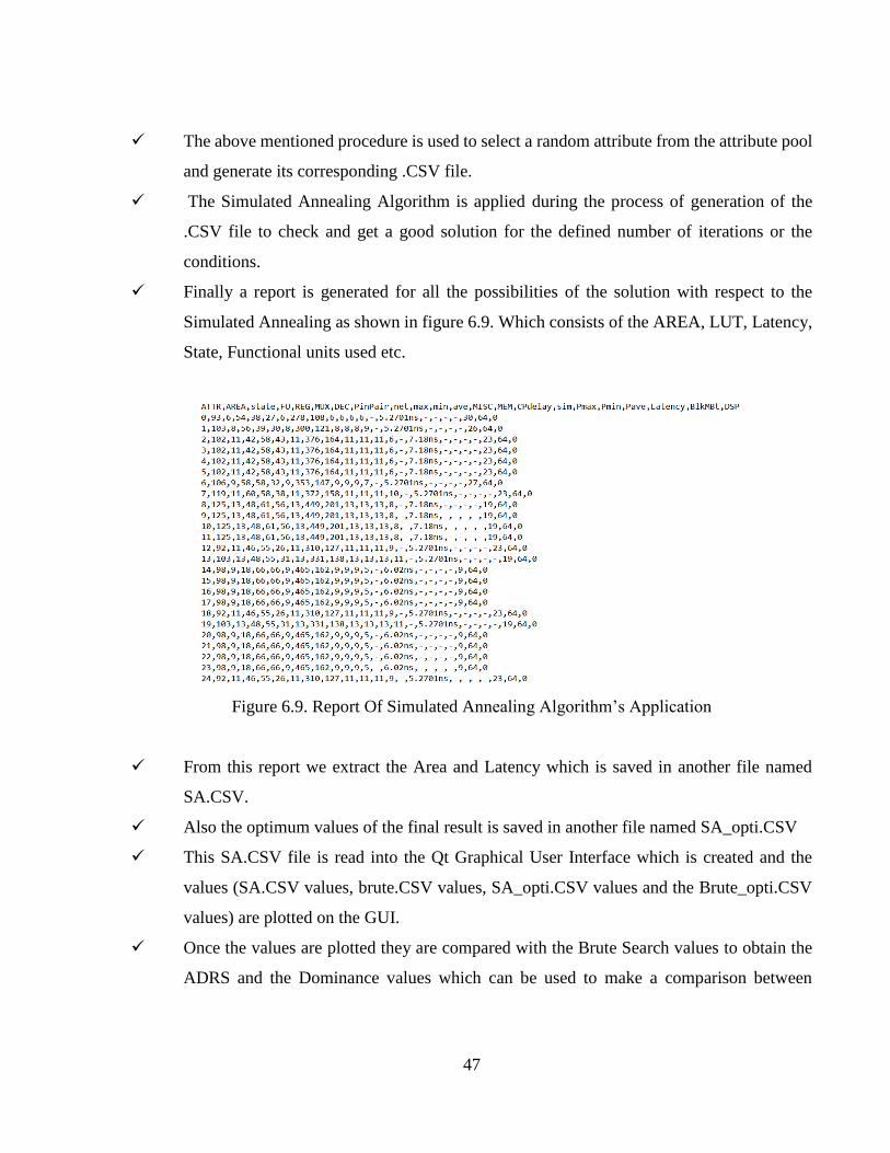
47
The above mentioned procedure is used to select a random attribute from the attribute pool
and generate its corresponding .CSV file.
The Simulated Annealing Algorithm is applied during the process of generation of the
.CSV file to check and get a good solution for the defined number of iterations or the
conditions.
Finally a report is generated for all the possibilities of the solution with respect to the
Simulated Annealing as shown in figure 6.9. Which consists of the AREA, LUT, Latency,
State, Functional units used etc.
Figure 6.9. Report Of Simulated Annealing Algorithm’s Application
From this report we extract the Area and Latency which is saved in another file named
SA.CSV.
Also the optimum values of the final result is saved in another file named SA_opti.CSV
This SA.CSV file is read into the Qt Graphical User Interface which is created and the
values (SA.CSV values, brute.CSV values, SA_opti.CSV values and the Brute_opti.CSV
values) are plotted on the GUI.
Once the values are plotted they are compared with the Brute Search values to obtain the
ADRS and the Dominance values which can be used to make a comparison between
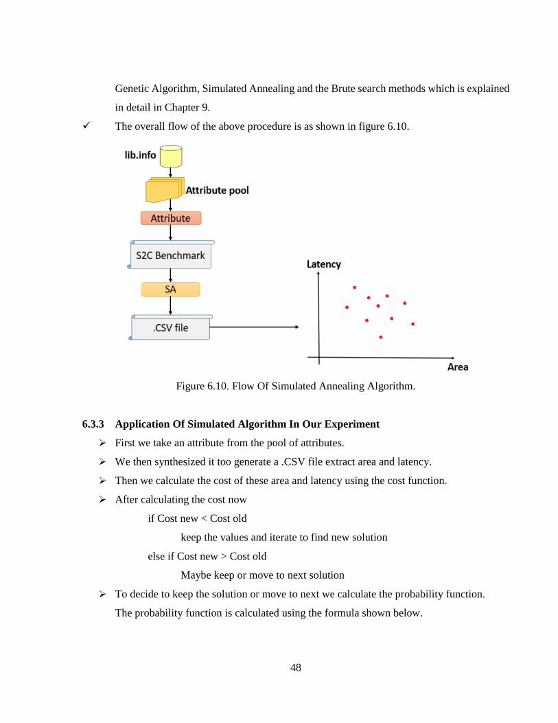
48
Genetic Algorithm, Simulated Annealing and the Brute search methods which is explained
in detail in Chapter 9.
The overall flow of the above procedure is as shown in figure 6.10.
Figure 6.10. Flow Of Simulated Annealing Algorithm.
6.3.3 Application Of Simulated Algorithm In Our Experiment
First we take an attribute from the pool of attributes.
We then synthesized it too generate a .CSV file extract area and latency.
Then we calculate the cost of these area and latency using the cost function.
After calculating the cost now
if Cost new < Cost old
keep the values and iterate to find new solution
else if Cost new > Cost old
Maybe keep or move to next solution
To decide to keep the solution or move to next we calculate the probability function.
The probability function is calculated using the formula shown below.
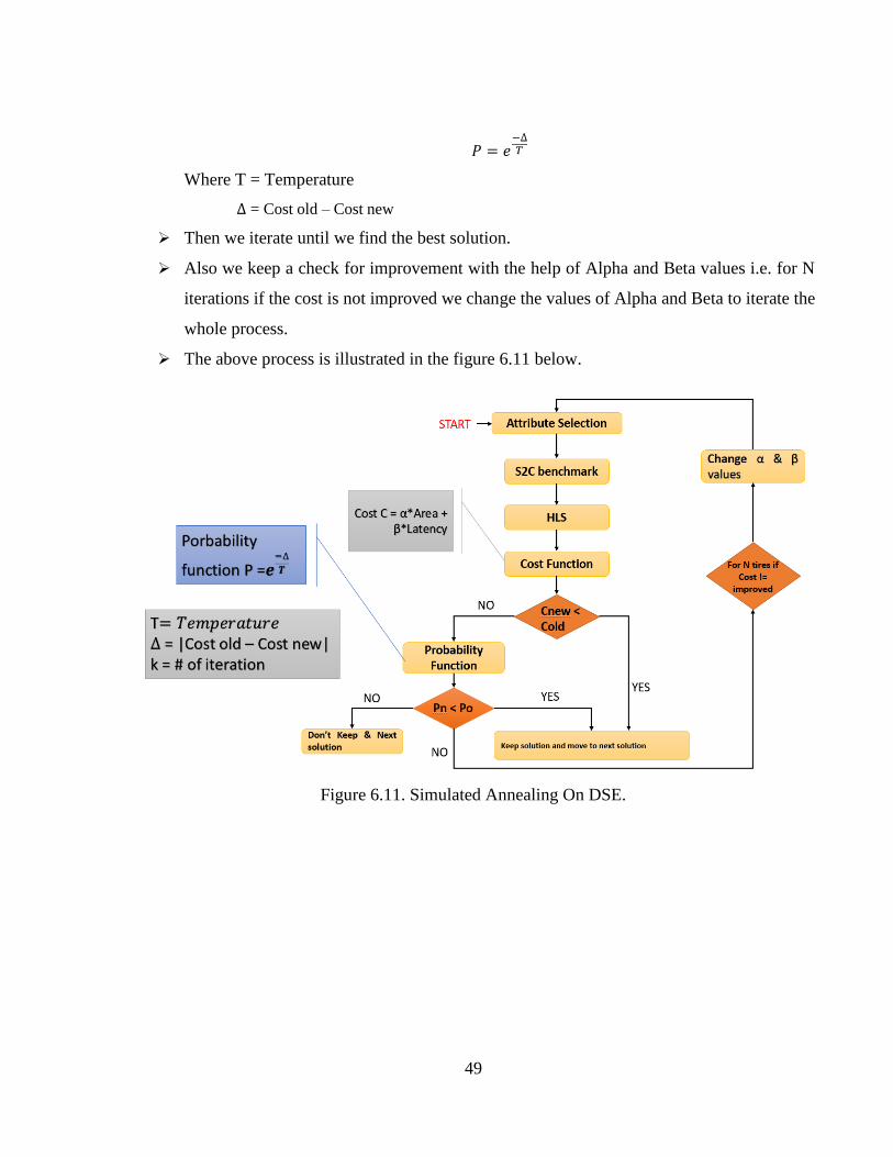
49
𝑃 = 𝑒−∆𝑇
Where T = Temperature
∆ = Cost old – Cost new
Then we iterate until we find the best solution.
Also we keep a check for improvement with the help of Alpha and Beta values i.e. for N
iterations if the cost is not improved we change the values of Alpha and Beta to iterate the
whole process.
The above process is illustrated in the figure 6.11 below.
Figure 6.11. Simulated Annealing On DSE.
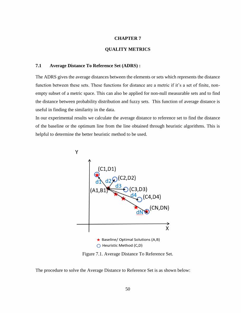
50
CHAPTER 7
QUALITY METRICS
7.1 Average Distance To Reference Set (ADRS) :
The ADRS gives the average distances between the elements or sets which represents the distance
function between these sets. These functions for distance are a metric if it’s a set of finite, non-
empty subset of a metric space. This can also be applied for non-null measurable sets and to find
the distance between probability distribution and fuzzy sets. This function of average distance is
useful in finding the similarity in the data.
In our experimental results we calculate the average distance to reference set to find the distance
of the baseline or the optimum line from the line obtained through heuristic algorithms. This is
helpful to determine the better heuristic method to be used.
Figure 7.1. Average Distance To Reference Set.
The procedure to solve the Average Distance to Reference Set is as shown below:
51
From the figure 7.1 we observer that A, B are the Optimal line points; C and D are a set of the
Heuristic data points.
Now we calculate ADRS with respect to these points on the graph obtained after the experimental
results are plotted on the GUI.
Where:
M= Number of Point in the Heuristic Method.
N= Number of points in the Optimal solution.
1. Step1:
First we calculate the distances d1(A1,B1), d2(A1,B1), d3(A1,B1) ……….. dN(A1,B1)
for all the points on the Heuristic curve using equation(1) as shown below,
d1(A1, B1) = {√(A1 − C1)2+(B1 − D1)2
d2(A1, B1) = {√(A1 − C2)2+(B1 − D2)2}
d3(A1, B1) = {√(A1 − C3)2+(B1 − D3)2}
………
dN(A1, B1) = {√(A1 − CN)2+(B1 − DN)2} (7.1)
2. Step2:
After we find the distances we find the minimum value of all the distances and store it in
Dist(A1,B1). We perform this step for all the points on the curve.
Dist(A1, B1) = Min{d1, d2, d3 … , dN} (7.2)
3. Step3:
Finally we calculate the Average distance to reference set using the below formula.
ADRS =∑ Dist(Ak,Bk)M
k=1
M (7.3)
7.2 Application Of ADRS On Our Results:
We implement the above stated procedure of calculating the ADRS in our GUI as shown in the
following figures 7.2 to 7.5.
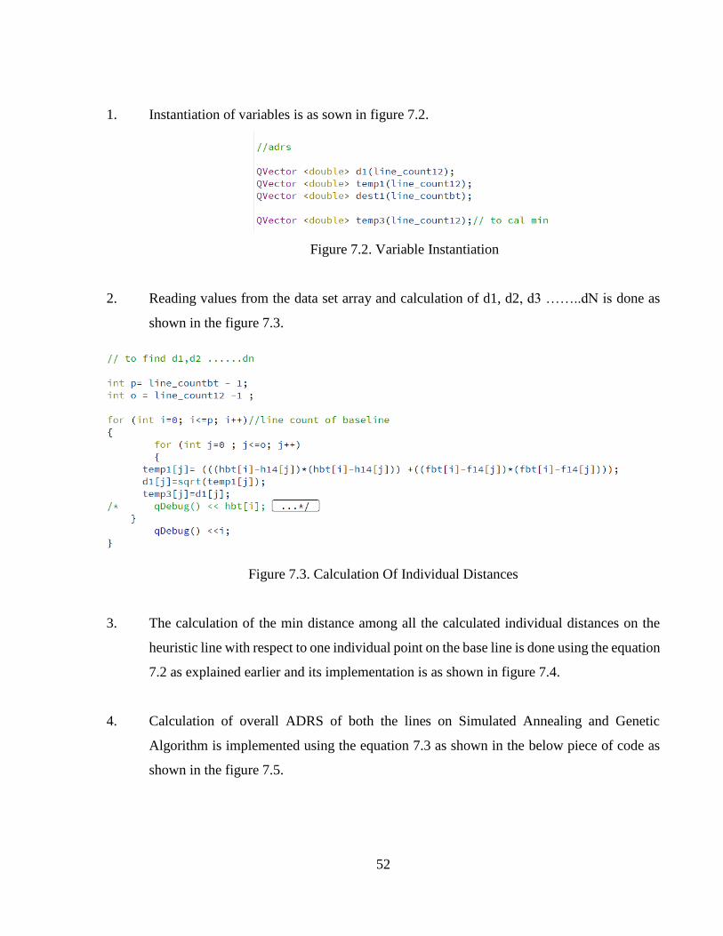
52
1. Instantiation of variables is as sown in figure 7.2.
Figure 7.2. Variable Instantiation
2. Reading values from the data set array and calculation of d1, d2, d3 ……..dN is done as
shown in the figure 7.3.
Figure 7.3. Calculation Of Individual Distances
3. The calculation of the min distance among all the calculated individual distances on the
heuristic line with respect to one individual point on the base line is done using the equation
7.2 as explained earlier and its implementation is as shown in figure 7.4.
4. Calculation of overall ADRS of both the lines on Simulated Annealing and Genetic
Algorithm is implemented using the equation 7.3 as shown in the below piece of code as
shown in the figure 7.5.
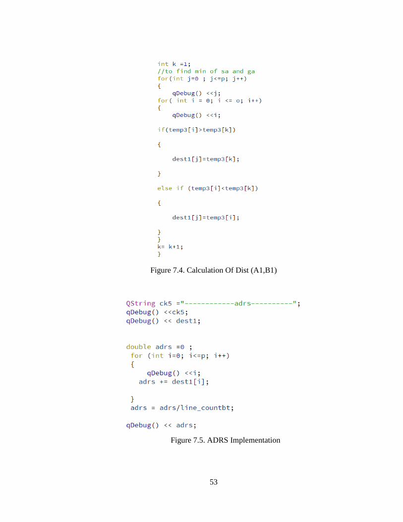
53
Figure 7.4. Calculation Of Dist (A1,B1)
Figure 7.5. ADRS Implementation
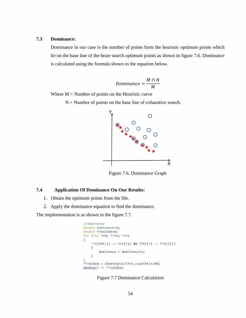
54
7.3 Dominance:
Dominance in our case is the number of points form the heuristic optimum points which
lie on the base line of the brute search optimum points as shown in figure 7.6. Dominance
is calculated using the formula shown in the equation below.
𝐷𝑜𝑚𝑖𝑛𝑎𝑛𝑐𝑒 =𝑀 ∩ 𝑁
𝑀
Where M = Number of points on the Heuristic curve
N = Number of points on the base line of exhaustive search.
Figure 7.6. Dominance Graph
7.4 Application Of Dominance On Our Results:
1. Obtain the optimum points from the file.
2. Apply the dominance equation to find the dominance.
The implementation is as shown in the figure 7.7.
Figure 7.7 Dominance Calculation
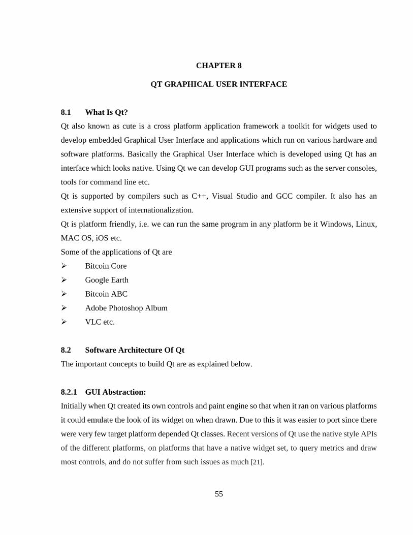
55
CHAPTER 8
QT GRAPHICAL USER INTERFACE
8.1 What Is Qt?
Qt also known as cute is a cross platform application framework a toolkit for widgets used to
develop embedded Graphical User Interface and applications which run on various hardware and
software platforms. Basically the Graphical User Interface which is developed using Qt has an
interface which looks native. Using Qt we can develop GUI programs such as the server consoles,
tools for command line etc.
Qt is supported by compilers such as C++, Visual Studio and GCC compiler. It also has an
extensive support of internationalization.
Qt is platform friendly, i.e. we can run the same program in any platform be it Windows, Linux,
MAC OS, iOS etc.
Some of the applications of Qt are
Bitcoin Core
Google Earth
Bitcoin ABC
Adobe Photoshop Album
VLC etc.
8.2 Software Architecture Of Qt
The important concepts to build Qt are as explained below.
8.2.1 GUI Abstraction:
Initially when Qt created its own controls and paint engine so that when it ran on various platforms
it could emulate the look of its widget on when drawn. Due to this it was easier to port since there
were very few target platform depended Qt classes. Recent versions of Qt use the native style APIs
of the different platforms, on platforms that have a native widget set, to query metrics and draw
most controls, and do not suffer from such issues as much [21].
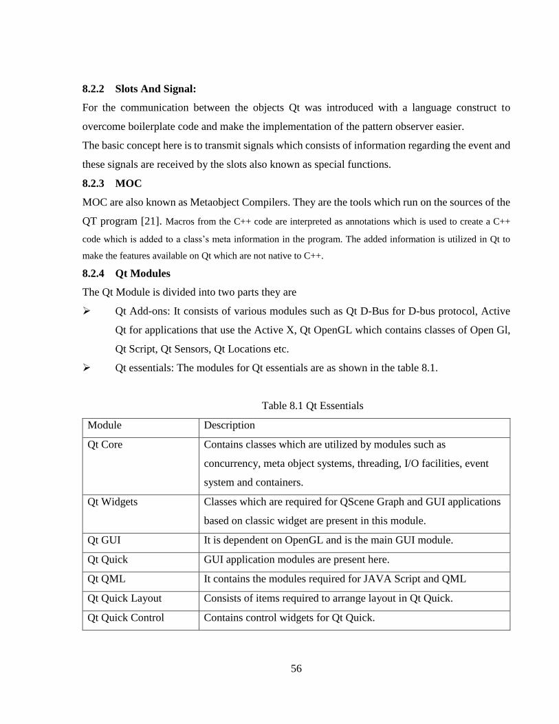
56
8.2.2 Slots And Signal:
For the communication between the objects Qt was introduced with a language construct to
overcome boilerplate code and make the implementation of the pattern observer easier.
The basic concept here is to transmit signals which consists of information regarding the event and
these signals are received by the slots also known as special functions.
8.2.3 MOC
MOC are also known as Metaobject Compilers. They are the tools which run on the sources of the
QT program [21]. Macros from the C++ code are interpreted as annotations which is used to create a C++
code which is added to a class’s meta information in the program. The added information is utilized in Qt to
make the features available on Qt which are not native to C++.
8.2.4 Qt Modules
The Qt Module is divided into two parts they are
Qt Add-ons: It consists of various modules such as Qt D-Bus for D-bus protocol, Active
Qt for applications that use the Active X, Qt OpenGL which contains classes of Open Gl,
Qt Script, Qt Sensors, Qt Locations etc.
Qt essentials: The modules for Qt essentials are as shown in the table 8.1.
Table 8.1 Qt Essentials
Module Description
Qt Core Contains classes which are utilized by modules such as
concurrency, meta object systems, threading, I/O facilities, event
system and containers.
Qt Widgets Classes which are required for QScene Graph and GUI applications
based on classic widget are present in this module.
Qt GUI It is dependent on OpenGL and is the main GUI module.
Qt Quick GUI application modules are present here.
Qt QML It contains the modules required for JAVA Script and QML
Qt Quick Layout Consists of items required to arrange layout in Qt Quick.
Qt Quick Control Contains control widgets for Qt Quick.
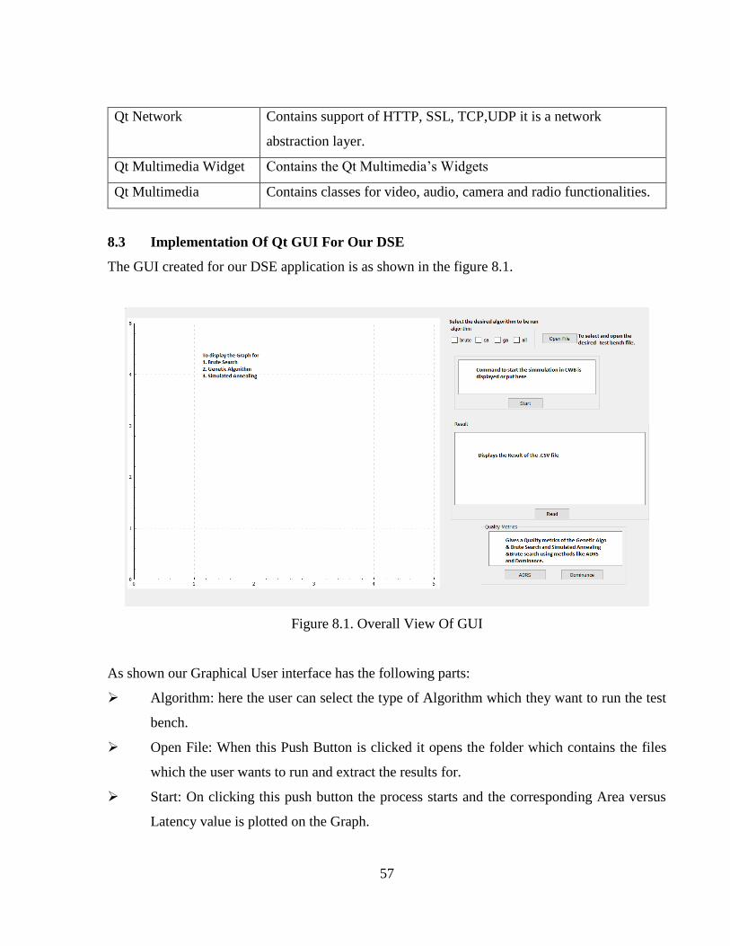
57
Qt Network Contains support of HTTP, SSL, TCP,UDP it is a network
abstraction layer.
Qt Multimedia Widget Contains the Qt Multimedia’s Widgets
Qt Multimedia Contains classes for video, audio, camera and radio functionalities.
8.3 Implementation Of Qt GUI For Our DSE
The GUI created for our DSE application is as shown in the figure 8.1.
Figure 8.1. Overall View Of GUI
As shown our Graphical User interface has the following parts:
Algorithm: here the user can select the type of Algorithm which they want to run the test
bench.
Open File: When this Push Button is clicked it opens the folder which contains the files
which the user wants to run and extract the results for.
Start: On clicking this push button the process starts and the corresponding Area versus
Latency value is plotted on the Graph.

58
Result: This Text editor displays the results in the .CSV file.
Quality Metric: on clicking the push button ADRS and Dominance the values are
calculated and displayed on the text editor window.
This is the complete overview of the Graphical User Interface built of our application using the
Modules which are specified above in table 8.1.
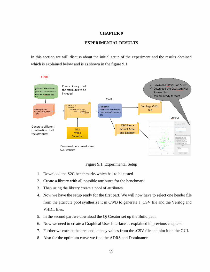
59
CHAPTER 9
EXPERIMENTAL RESULTS
In this section we will discuss about the initial setup of the experiment and the results obtained
which is explained below and is as shown in the figure 9.1.
Figure 9.1. Experimental Setup
1. Download the S2C benchmarks which has to be tested.
2. Create a library with all possible attributes for the benchmark
3. Then using the library create a pool of attributes.
4. Now we have the setup ready for the first part. We will now have to select one header file
from the attribute pool synthesize it in CWB to generate a .CSV file and the Verilog and
VHDL files.
5. In the second part we download the Qt Creator set up the Build path.
6. Now we need to create a Graphical User Interface as explained in previous chapters.
7. Further we extract the area and latency values from the .CSV file and plot it on the GUI.
8. Also for the optimum curve we find the ADRS and Dominance.
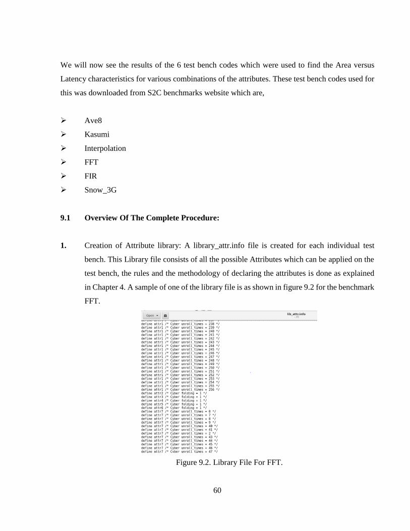
60
We will now see the results of the 6 test bench codes which were used to find the Area versus
Latency characteristics for various combinations of the attributes. These test bench codes used for
this was downloaded from S2C benchmarks website which are,
Ave8
Kasumi
Interpolation
FFT
FIR
Snow_3G
9.1 Overview Of The Complete Procedure:
1. Creation of Attribute library: A library_attr.info file is created for each individual test
bench. This Library file consists of all the possible Attributes which can be applied on the
test bench, the rules and the methodology of declaring the attributes is done as explained
in Chapter 4. A sample of one of the library file is as shown in figure 9.2 for the benchmark
FFT.
Figure 9.2. Library File For FFT.
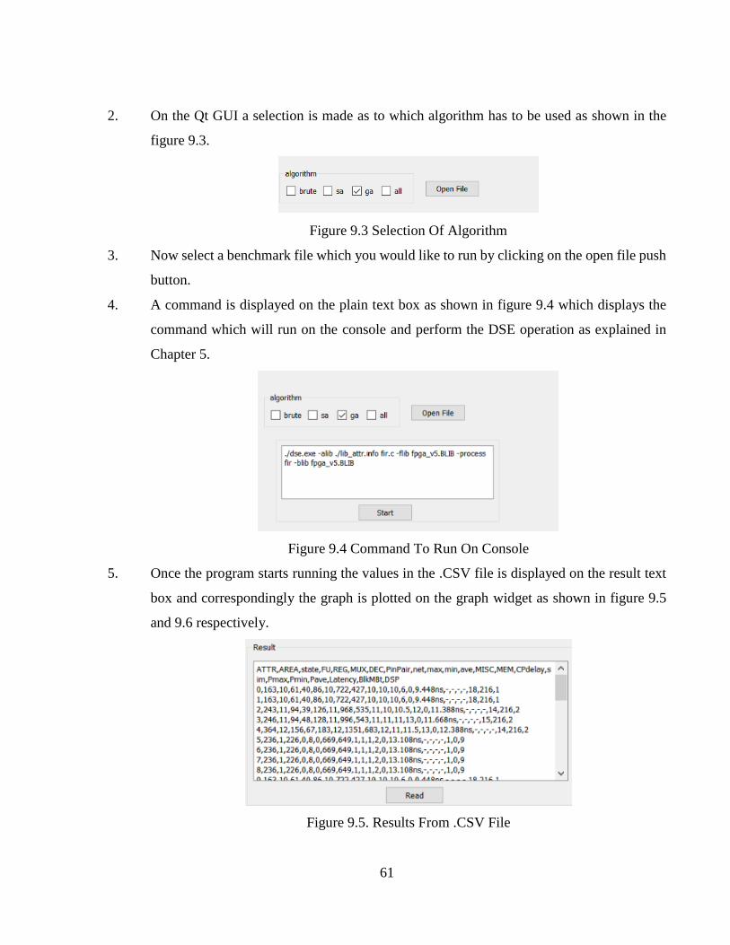
61
2. On the Qt GUI a selection is made as to which algorithm has to be used as shown in the
figure 9.3.
Figure 9.3 Selection Of Algorithm
3. Now select a benchmark file which you would like to run by clicking on the open file push
button.
4. A command is displayed on the plain text box as shown in figure 9.4 which displays the
command which will run on the console and perform the DSE operation as explained in
Chapter 5.
Figure 9.4 Command To Run On Console
5. Once the program starts running the values in the .CSV file is displayed on the result text
box and correspondingly the graph is plotted on the graph widget as shown in figure 9.5
and 9.6 respectively.
Figure 9.5. Results From .CSV File
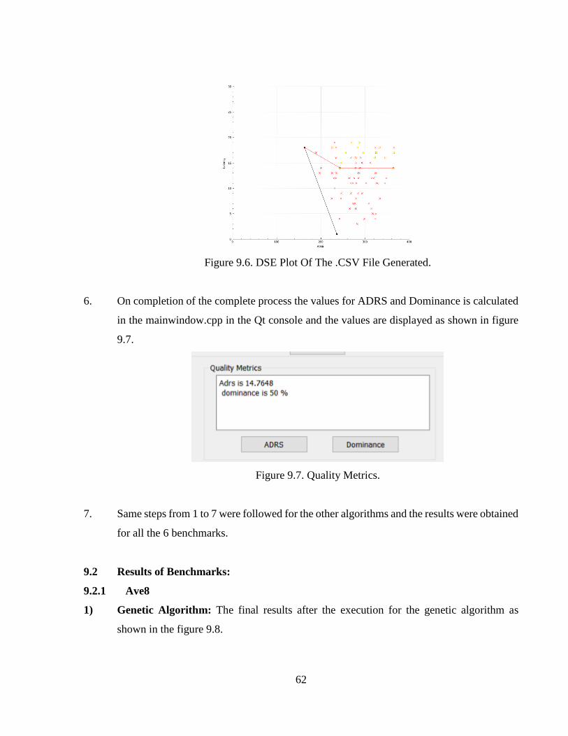
62
Figure 9.6. DSE Plot Of The .CSV File Generated.
6. On completion of the complete process the values for ADRS and Dominance is calculated
in the mainwindow.cpp in the Qt console and the values are displayed as shown in figure
9.7.
Figure 9.7. Quality Metrics.
7. Same steps from 1 to 7 were followed for the other algorithms and the results were obtained
for all the 6 benchmarks.
9.2 Results of Benchmarks:
9.2.1 Ave8
1) Genetic Algorithm: The final results after the execution for the genetic algorithm as
shown in the figure 9.8.
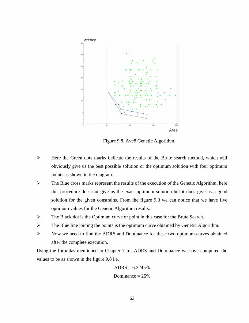
63
Figure 9.8. Ave8 Genetic Algorithm.
Here the Green dots marks indicate the results of the Brute search method, which will
obviously give us the best possible solution or the optimum solution with four optimum
points as shown in the diagram.
The Blue cross marks represent the results of the execution of the Genetic Algorithm, here
this procedure does not give us the exact optimum solution but it does give us a good
solution for the given constrains. From the figure 9.8 we can notice that we have five
optimum values for the Genetic Algorithm results.
The Black dot is the Optimum curve or point in this case for the Brute Search.
The Blue line joining the points is the optimum curve obtained by Genetic Algorithm.
Now we need to find the ADRS and Dominance for these two optimum curves obtained
after the complete execution.
Using the formulas mentioned in Chapter 7 for ADRS and Dominance we have computed the
values to be as shown in the figure 9.8 i.e.
ADRS = 6.3245%
Dominance = 25%
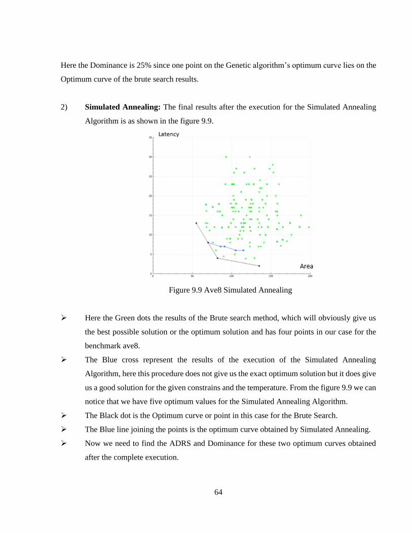
64
Here the Dominance is 25% since one point on the Genetic algorithm’s optimum curve lies on the
Optimum curve of the brute search results.
2) Simulated Annealing: The final results after the execution for the Simulated Annealing
Algorithm is as shown in the figure 9.9.
Figure 9.9 Ave8 Simulated Annealing
Here the Green dots the results of the Brute search method, which will obviously give us
the best possible solution or the optimum solution and has four points in our case for the
benchmark ave8.
The Blue cross represent the results of the execution of the Simulated Annealing
Algorithm, here this procedure does not give us the exact optimum solution but it does give
us a good solution for the given constrains and the temperature. From the figure 9.9 we can
notice that we have five optimum values for the Simulated Annealing Algorithm.
The Black dot is the Optimum curve or point in this case for the Brute Search.
The Blue line joining the points is the optimum curve obtained by Simulated Annealing.
Now we need to find the ADRS and Dominance for these two optimum curves obtained
after the complete execution.
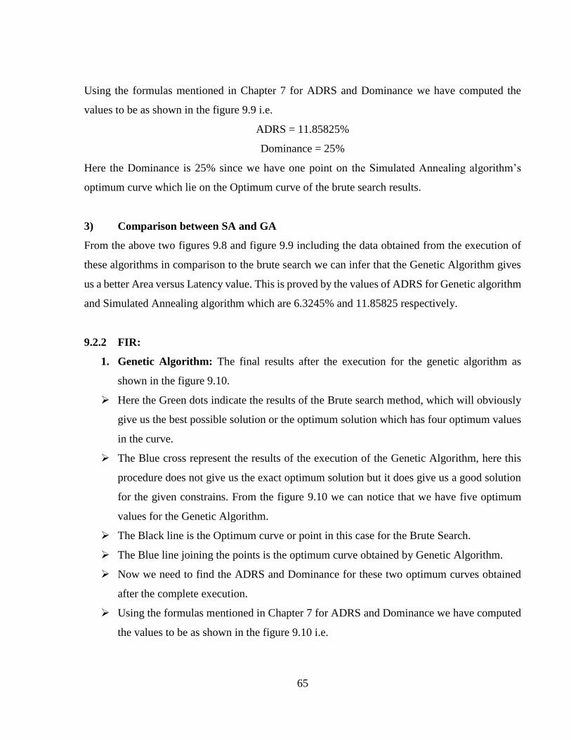
65
Using the formulas mentioned in Chapter 7 for ADRS and Dominance we have computed the
values to be as shown in the figure 9.9 i.e.
ADRS = 11.85825%
Dominance = 25%
Here the Dominance is 25% since we have one point on the Simulated Annealing algorithm’s
optimum curve which lie on the Optimum curve of the brute search results.
3) Comparison between SA and GA
From the above two figures 9.8 and figure 9.9 including the data obtained from the execution of
these algorithms in comparison to the brute search we can infer that the Genetic Algorithm gives
us a better Area versus Latency value. This is proved by the values of ADRS for Genetic algorithm
and Simulated Annealing algorithm which are 6.3245% and 11.85825 respectively.
9.2.2 FIR:
1. Genetic Algorithm: The final results after the execution for the genetic algorithm as
shown in the figure 9.10.
Here the Green dots indicate the results of the Brute search method, which will obviously
give us the best possible solution or the optimum solution which has four optimum values
in the curve.
The Blue cross represent the results of the execution of the Genetic Algorithm, here this
procedure does not give us the exact optimum solution but it does give us a good solution
for the given constrains. From the figure 9.10 we can notice that we have five optimum
values for the Genetic Algorithm.
The Black line is the Optimum curve or point in this case for the Brute Search.
The Blue line joining the points is the optimum curve obtained by Genetic Algorithm.
Now we need to find the ADRS and Dominance for these two optimum curves obtained
after the complete execution.
Using the formulas mentioned in Chapter 7 for ADRS and Dominance we have computed
the values to be as shown in the figure 9.10 i.e.
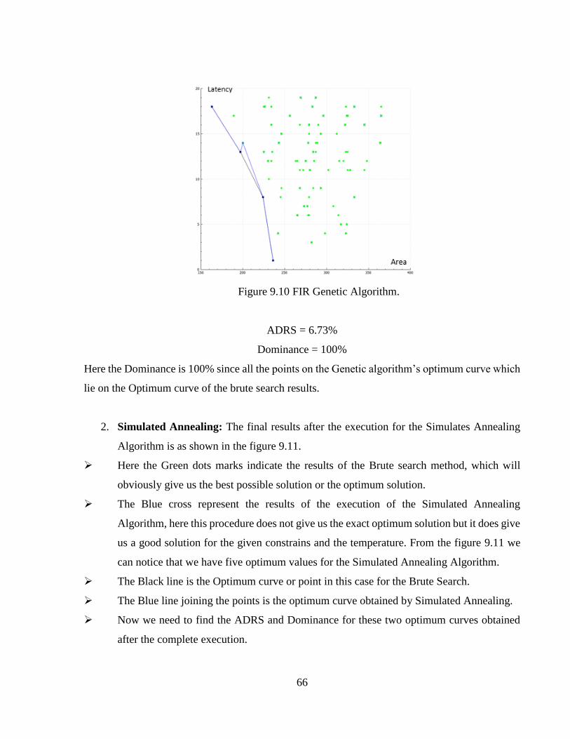
66
Figure 9.10 FIR Genetic Algorithm.
ADRS = 6.73%
Dominance = 100%
Here the Dominance is 100% since all the points on the Genetic algorithm’s optimum curve which
lie on the Optimum curve of the brute search results.
2. Simulated Annealing: The final results after the execution for the Simulates Annealing
Algorithm is as shown in the figure 9.11.
Here the Green dots marks indicate the results of the Brute search method, which will
obviously give us the best possible solution or the optimum solution.
The Blue cross represent the results of the execution of the Simulated Annealing
Algorithm, here this procedure does not give us the exact optimum solution but it does give
us a good solution for the given constrains and the temperature. From the figure 9.11 we
can notice that we have five optimum values for the Simulated Annealing Algorithm.
The Black line is the Optimum curve or point in this case for the Brute Search.
The Blue line joining the points is the optimum curve obtained by Simulated Annealing.
Now we need to find the ADRS and Dominance for these two optimum curves obtained
after the complete execution.
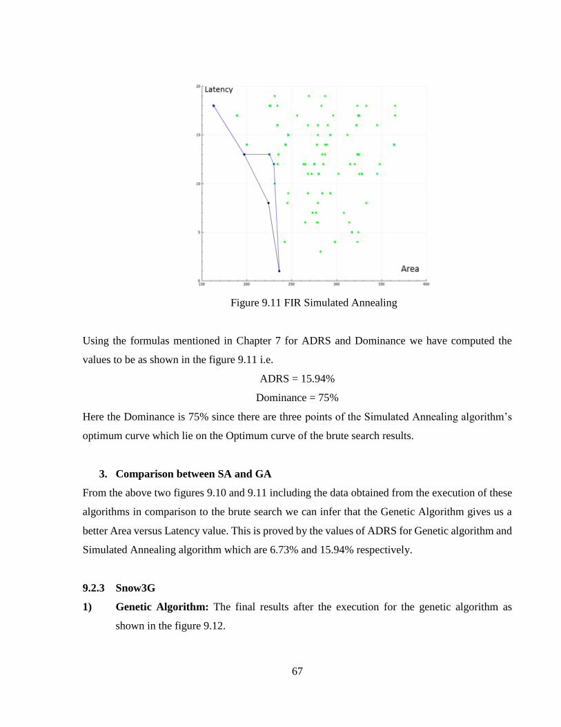
67
Figure 9.11 FIR Simulated Annealing
Using the formulas mentioned in Chapter 7 for ADRS and Dominance we have computed the
values to be as shown in the figure 9.11 i.e.
ADRS = 15.94%
Dominance = 75%
Here the Dominance is 75% since there are three points of the Simulated Annealing algorithm’s
optimum curve which lie on the Optimum curve of the brute search results.
3. Comparison between SA and GA
From the above two figures 9.10 and 9.11 including the data obtained from the execution of these
algorithms in comparison to the brute search we can infer that the Genetic Algorithm gives us a
better Area versus Latency value. This is proved by the values of ADRS for Genetic algorithm and
Simulated Annealing algorithm which are 6.73% and 15.94% respectively.
9.2.3 Snow3G
1) Genetic Algorithm: The final results after the execution for the genetic algorithm as
shown in the figure 9.12.
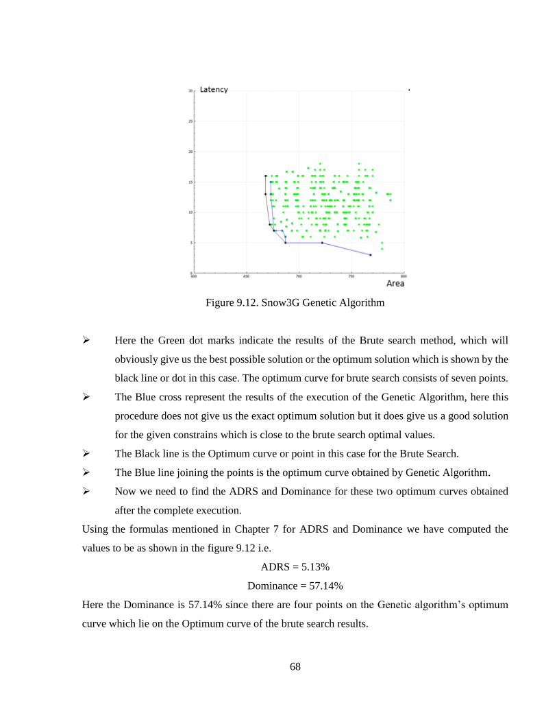
68
Figure 9.12. Snow3G Genetic Algorithm
Here the Green dot marks indicate the results of the Brute search method, which will
obviously give us the best possible solution or the optimum solution which is shown by the
black line or dot in this case. The optimum curve for brute search consists of seven points.
The Blue cross represent the results of the execution of the Genetic Algorithm, here this
procedure does not give us the exact optimum solution but it does give us a good solution
for the given constrains which is close to the brute search optimal values.
The Black line is the Optimum curve or point in this case for the Brute Search.
The Blue line joining the points is the optimum curve obtained by Genetic Algorithm.
Now we need to find the ADRS and Dominance for these two optimum curves obtained
after the complete execution.
Using the formulas mentioned in Chapter 7 for ADRS and Dominance we have computed the
values to be as shown in the figure 9.12 i.e.
ADRS = 5.13%
Dominance = 57.14%
Here the Dominance is 57.14% since there are four points on the Genetic algorithm’s optimum
curve which lie on the Optimum curve of the brute search results.
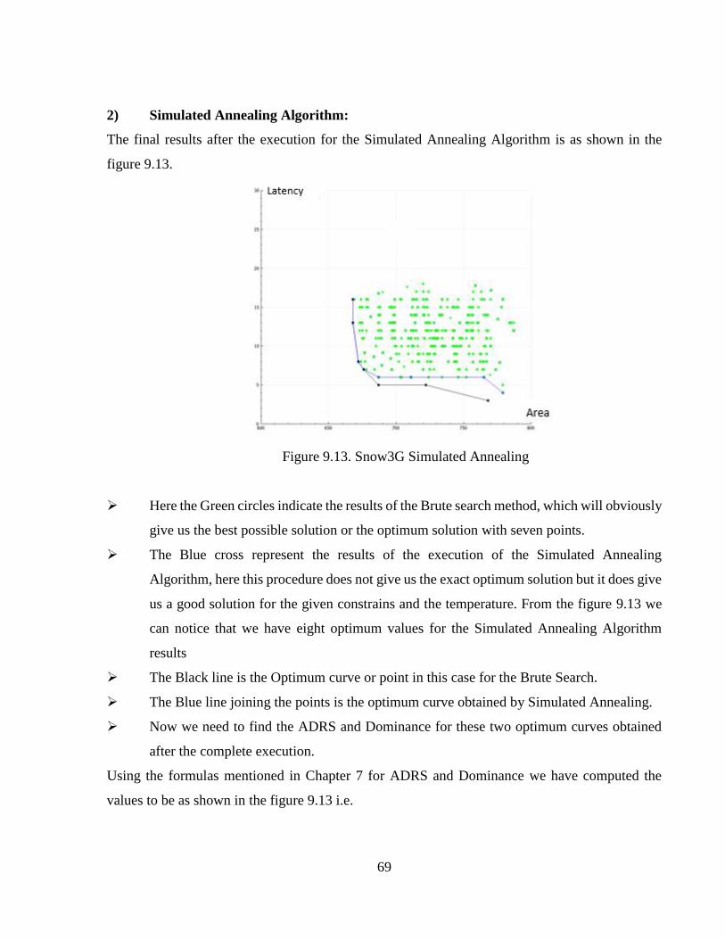
69
2) Simulated Annealing Algorithm:
The final results after the execution for the Simulated Annealing Algorithm is as shown in the
figure 9.13.
Figure 9.13. Snow3G Simulated Annealing
Here the Green circles indicate the results of the Brute search method, which will obviously
give us the best possible solution or the optimum solution with seven points.
The Blue cross represent the results of the execution of the Simulated Annealing
Algorithm, here this procedure does not give us the exact optimum solution but it does give
us a good solution for the given constrains and the temperature. From the figure 9.13 we
can notice that we have eight optimum values for the Simulated Annealing Algorithm
results
The Black line is the Optimum curve or point in this case for the Brute Search.
The Blue line joining the points is the optimum curve obtained by Simulated Annealing.
Now we need to find the ADRS and Dominance for these two optimum curves obtained
after the complete execution.
Using the formulas mentioned in Chapter 7 for ADRS and Dominance we have computed the
values to be as shown in the figure 9.13 i.e.
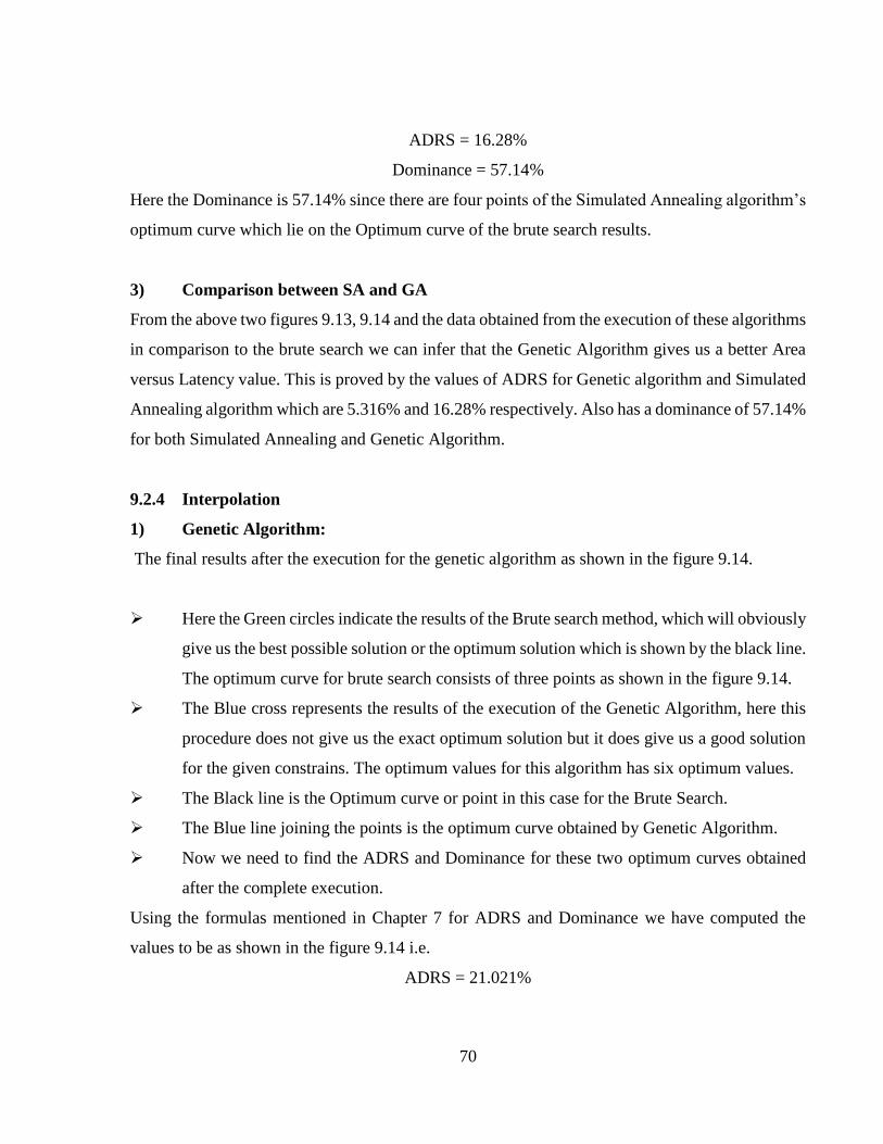
70
ADRS = 16.28%
Dominance = 57.14%
Here the Dominance is 57.14% since there are four points of the Simulated Annealing algorithm’s
optimum curve which lie on the Optimum curve of the brute search results.
3) Comparison between SA and GA
From the above two figures 9.13, 9.14 and the data obtained from the execution of these algorithms
in comparison to the brute search we can infer that the Genetic Algorithm gives us a better Area
versus Latency value. This is proved by the values of ADRS for Genetic algorithm and Simulated
Annealing algorithm which are 5.316% and 16.28% respectively. Also has a dominance of 57.14%
for both Simulated Annealing and Genetic Algorithm.
9.2.4 Interpolation
1) Genetic Algorithm:
The final results after the execution for the genetic algorithm as shown in the figure 9.14.
Here the Green circles indicate the results of the Brute search method, which will obviously
give us the best possible solution or the optimum solution which is shown by the black line.
The optimum curve for brute search consists of three points as shown in the figure 9.14.
The Blue cross represents the results of the execution of the Genetic Algorithm, here this
procedure does not give us the exact optimum solution but it does give us a good solution
for the given constrains. The optimum values for this algorithm has six optimum values.
The Black line is the Optimum curve or point in this case for the Brute Search.
The Blue line joining the points is the optimum curve obtained by Genetic Algorithm.
Now we need to find the ADRS and Dominance for these two optimum curves obtained
after the complete execution.
Using the formulas mentioned in Chapter 7 for ADRS and Dominance we have computed the
values to be as shown in the figure 9.14 i.e.
ADRS = 21.021%
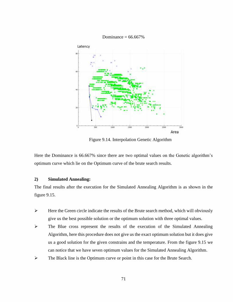
71
Dominance = 66.667%
Figure 9.14. Interpolation Genetic Algorithm
Here the Dominance is 66.667% since there are two optimal values on the Genetic algorithm’s
optimum curve which lie on the Optimum curve of the brute search results.
2) Simulated Annealing:
The final results after the execution for the Simulated Annealing Algorithm is as shown in the
figure 9.15.
Here the Green circle indicate the results of the Brute search method, which will obviously
give us the best possible solution or the optimum solution with three optimal values.
The Blue cross represent the results of the execution of the Simulated Annealing
Algorithm, here this procedure does not give us the exact optimum solution but it does give
us a good solution for the given constrains and the temperature. From the figure 9.15 we
can notice that we have seven optimum values for the Simulated Annealing Algorithm.
The Black line is the Optimum curve or point in this case for the Brute Search.
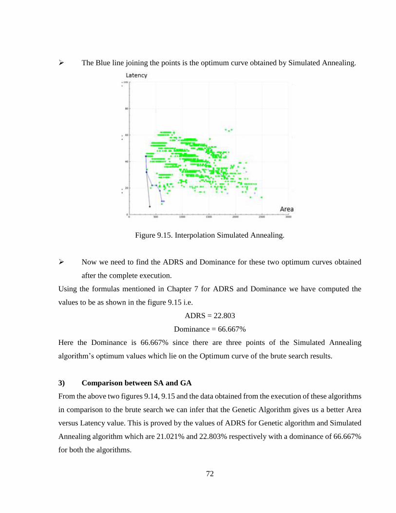
72
The Blue line joining the points is the optimum curve obtained by Simulated Annealing.
Figure 9.15. Interpolation Simulated Annealing.
Now we need to find the ADRS and Dominance for these two optimum curves obtained
after the complete execution.
Using the formulas mentioned in Chapter 7 for ADRS and Dominance we have computed the
values to be as shown in the figure 9.15 i.e.
ADRS = 22.803
Dominance = 66.667%
Here the Dominance is 66.667% since there are three points of the Simulated Annealing
algorithm’s optimum values which lie on the Optimum curve of the brute search results.
3) Comparison between SA and GA
From the above two figures 9.14, 9.15 and the data obtained from the execution of these algorithms
in comparison to the brute search we can infer that the Genetic Algorithm gives us a better Area
versus Latency value. This is proved by the values of ADRS for Genetic algorithm and Simulated
Annealing algorithm which are 21.021% and 22.803% respectively with a dominance of 66.667%
for both the algorithms.
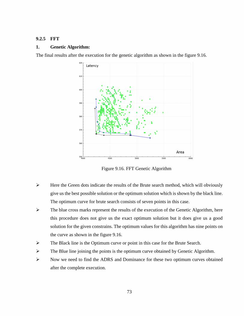
73
9.2.5 FFT
1. Genetic Algorithm:
The final results after the execution for the genetic algorithm as shown in the figure 9.16.
Figure 9.16. FFT Genetic Algorithm
Here the Green dots indicate the results of the Brute search method, which will obviously
give us the best possible solution or the optimum solution which is shown by the black line.
The optimum curve for brute search consists of seven points in this case.
The blue cross marks represent the results of the execution of the Genetic Algorithm, here
this procedure does not give us the exact optimum solution but it does give us a good
solution for the given constrains. The optimum values for this algorithm has nine points on
the curve as shown in the figure 9.16.
The Black line is the Optimum curve or point in this case for the Brute Search.
The Blue line joining the points is the optimum curve obtained by Genetic Algorithm.
Now we need to find the ADRS and Dominance for these two optimum curves obtained
after the complete execution.
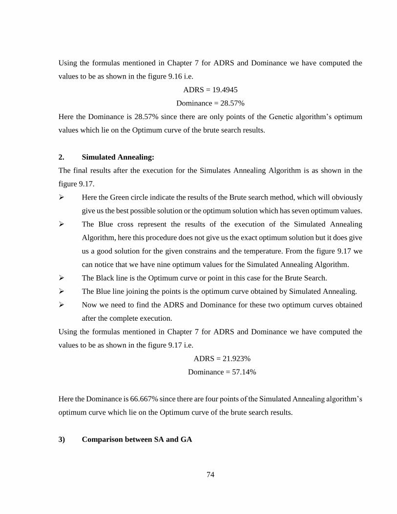
74
Using the formulas mentioned in Chapter 7 for ADRS and Dominance we have computed the
values to be as shown in the figure 9.16 i.e.
ADRS = 19.4945
Dominance = 28.57%
Here the Dominance is 28.57% since there are only points of the Genetic algorithm’s optimum
values which lie on the Optimum curve of the brute search results.
2. Simulated Annealing:
The final results after the execution for the Simulates Annealing Algorithm is as shown in the
figure 9.17.
Here the Green circle indicate the results of the Brute search method, which will obviously
give us the best possible solution or the optimum solution which has seven optimum values.
The Blue cross represent the results of the execution of the Simulated Annealing
Algorithm, here this procedure does not give us the exact optimum solution but it does give
us a good solution for the given constrains and the temperature. From the figure 9.17 we
can notice that we have nine optimum values for the Simulated Annealing Algorithm.
The Black line is the Optimum curve or point in this case for the Brute Search.
The Blue line joining the points is the optimum curve obtained by Simulated Annealing.
Now we need to find the ADRS and Dominance for these two optimum curves obtained
after the complete execution.
Using the formulas mentioned in Chapter 7 for ADRS and Dominance we have computed the
values to be as shown in the figure 9.17 i.e.
ADRS = 21.923%
Dominance = 57.14%
Here the Dominance is 66.667% since there are four points of the Simulated Annealing algorithm’s
optimum curve which lie on the Optimum curve of the brute search results.
3) Comparison between SA and GA
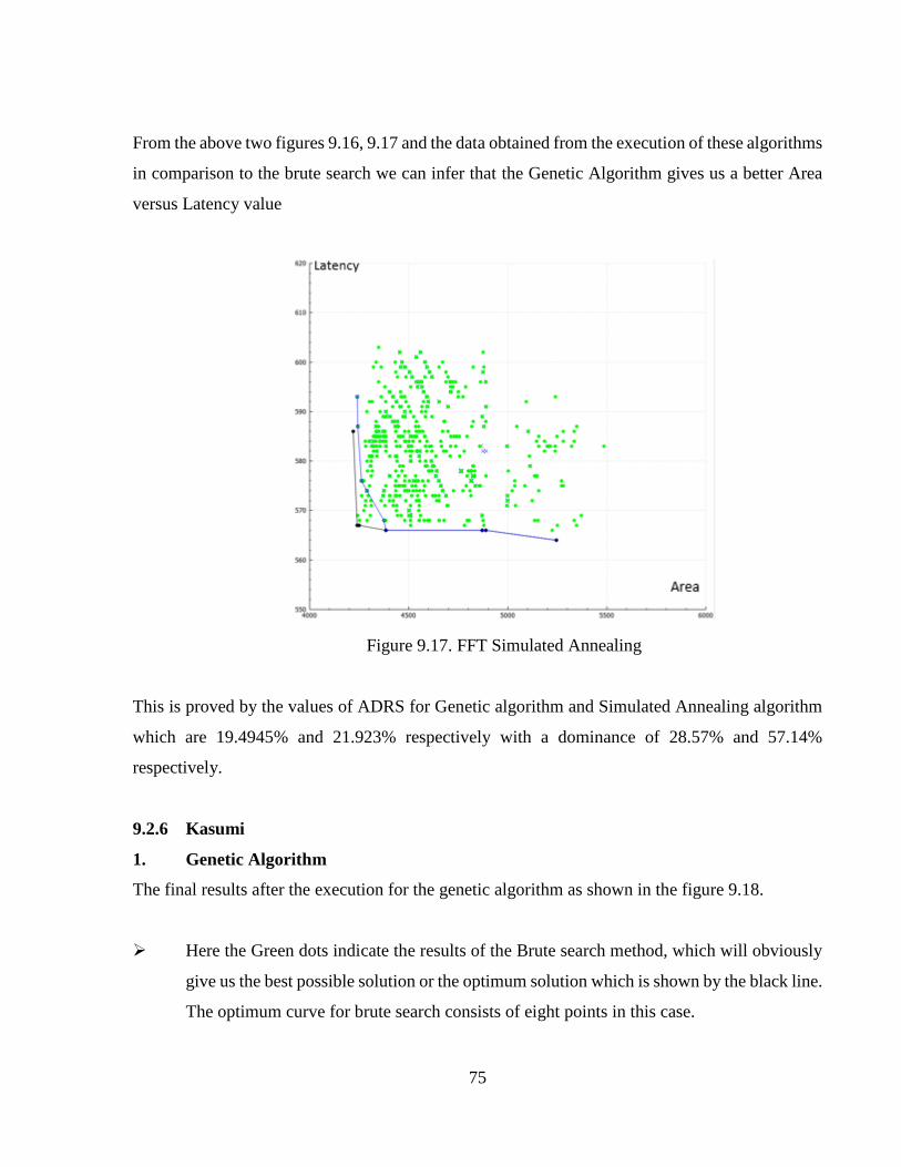
75
From the above two figures 9.16, 9.17 and the data obtained from the execution of these algorithms
in comparison to the brute search we can infer that the Genetic Algorithm gives us a better Area
versus Latency value
Figure 9.17. FFT Simulated Annealing
This is proved by the values of ADRS for Genetic algorithm and Simulated Annealing algorithm
which are 19.4945% and 21.923% respectively with a dominance of 28.57% and 57.14%
respectively.
9.2.6 Kasumi
1. Genetic Algorithm
The final results after the execution for the genetic algorithm as shown in the figure 9.18.
Here the Green dots indicate the results of the Brute search method, which will obviously
give us the best possible solution or the optimum solution which is shown by the black line.
The optimum curve for brute search consists of eight points in this case.
76
The blue cross marks represent the results of the execution of the Genetic Algorithm, here
this procedure does not give us the exact optimum solution but it does give us a good
solution for the given constrains. The optimum values for this algorithm has ten points on
the curve as shown in the figure 9.18.
Figure 9.18. Kasumi Genetic Algorithm
The Black line is the Optimum curve or point in this case for the Brute Search.
The Blue line joining the points is the optimum curve obtained by Genetic Algorithm.
Now we need to find the ADRS and Dominance for these two optimum curves obtained
after the complete execution.
Using the formulas mentioned in Chapter 7 for ADRS and Dominance we have computed the
values to be as shown in the figure 9.18 i.e.
ADRS = 8.3245%
Dominance = 75%
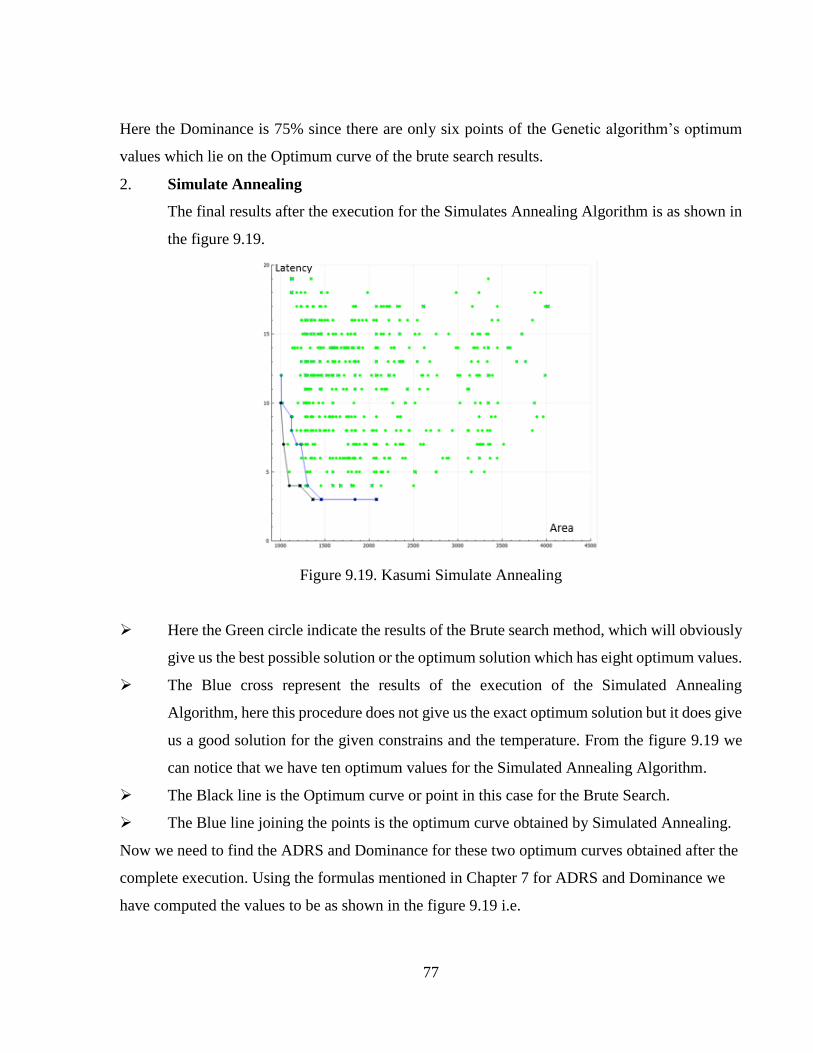
77
Here the Dominance is 75% since there are only six points of the Genetic algorithm’s optimum
values which lie on the Optimum curve of the brute search results.
2. Simulate Annealing
The final results after the execution for the Simulates Annealing Algorithm is as shown in
the figure 9.19.
Figure 9.19. Kasumi Simulate Annealing
Here the Green circle indicate the results of the Brute search method, which will obviously
give us the best possible solution or the optimum solution which has eight optimum values.
The Blue cross represent the results of the execution of the Simulated Annealing
Algorithm, here this procedure does not give us the exact optimum solution but it does give
us a good solution for the given constrains and the temperature. From the figure 9.19 we
can notice that we have ten optimum values for the Simulated Annealing Algorithm.
The Black line is the Optimum curve or point in this case for the Brute Search.
The Blue line joining the points is the optimum curve obtained by Simulated Annealing.
Now we need to find the ADRS and Dominance for these two optimum curves obtained after the
complete execution. Using the formulas mentioned in Chapter 7 for ADRS and Dominance we
have computed the values to be as shown in the figure 9.19 i.e.
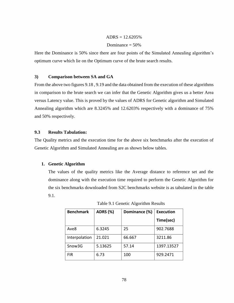
78
ADRS = 12.6205%
Dominance = 50%
Here the Dominance is 50% since there are four points of the Simulated Annealing algorithm’s
optimum curve which lie on the Optimum curve of the brute search results.
3) Comparison between SA and GA
From the above two figures 9.18 , 9.19 and the data obtained from the execution of these algorithms
in comparison to the brute search we can infer that the Genetic Algorithm gives us a better Area
versus Latency value. This is proved by the values of ADRS for Genetic algorithm and Simulated
Annealing algorithm which are 8.3245% and 12.6203% respectively with a dominance of 75%
and 50% respectively.
9.3 Results Tabulation:
The Quality metrics and the execution time for the above six benchmarks after the execution of
Genetic Algorithm and Simulated Annealing are as shown below tables.
1. Genetic Algorithm
The values of the quality metrics like the Average distance to reference set and the
dominance along with the execution time required to perform the Genetic Algorithm for
the six benchmarks downloaded from S2C benchmarks website is as tabulated in the table
9.1.
Table 9.1 Genetic Algorithm Results
Benchmark ADRS (%) Dominance (%) Execution
Time(sec)
Ave8 6.3245 25 902.7688
Interpolation 21.021 66.667 3211.86
Snow3G 5.13625 57.14 1397.13527
FIR 6.73 100 929.2471

79
FFT 19.4945 28.57 1588.87819
Kasumi 8.3245 75 1601.12725
2. Simulated Annealing
The values of the quality metrics like the Average distance to reference set and the dominance
along with the execution time required to perform the Genetic Algorithm for the six
benchmarks downloaded from S2C benchmarks website is as tabulated in the table 9.2.
Table 9.2 Simulated Annealing results
Benchmark ADRS (%) Dominance (%) Execution
Time(sec)
Ave8 11.85825 25 1116.252
Interpolation 22.803 66.667 3970.262829
Snow3G 16.28 57.14 1728.3409
FIR 15.94 75 1148.402
FFT 21.923 57.14 1964.3400
Kasumi 12.6205 50 1978.3967
From the above tabulation we can observe that Genetic Algorithm gives us a better optimal
solution with a lower execution time and lower dominance. But we have a tradeoff that if we
simulate the simulated annealing for a longer time period the chances of obtaining the best optimal
solution similar to the brute search results with respect to Genetic Algorithm. We observe from
the execution time that there is an increase of almost 20% in the execution time for simulated
annealing algorithm in comparison with genetic algorithm.
80
CHAPTER 10
CONCLUSION AND FUTURE WORK
10.1 Conclusion
In the first part of the thesis the S2C Benchmarks were tested for the three conditions i.e Exhaustive
Search or Brute Search, Genetic Algorithm and Simulated Annealing in order to find a better
optimum value for the given time and resource constrains. This was implemented using the GUI
which ran the Design Space Exploration for all the three algorithms on the Cyber Work Bench
tool. The resulting .CSV file was generated for each algorithm.
In the second part of the thesis from the .CSV file area and latency values were extracted and
plotted and analyzed on the GUI created. Techniques like ADRS and Dominance were used to
draw a conclusion that for all the benchmarks which were executed the Genetic Algorithm
provided a better result in comparison to Simulated Annealing Algorithm.
10.2 Future Work
The future scope of this research work can be executing these experiments on a huge range of
benchmarks. Also these benchmarks can be tested on various other Algorithms like Machine
Learning algorithms, other Heuristic Algorithms and even a new Algorithm can be developed to
obtain a near optimum solution for a given set of Attributes. There is a scope for optimizing the
area versus latency and other parameters using other Algorithms.
81
REFERENCES
[1] A.Sangiovanni Vincentelli, ‘The Tides of EDA,’’ IEEE Design & Test, vol. 20, no. 6,
2003, pp. 59-75.
[2] D. MacMillen et al., ‘‘An Industrial View of Electronic Design Automation,’’ IEEE
Trans. Computer-Aided Design of Integrated Circuits and Systems, vol. 19, no. 12, 2000,
pp. 1428-1448.
[3] D.W. Knapp, Behavioral Synthesis: Digital System Design Using the Synopsys Behavioral
Compiler, Prentice Hall, 1996.
[4] J.P. Elliot, Understanding Behavioral Synthesis: A Practical Guide to High-Level Design,
Kluwer Academic Publishers, 1999.
[5] B. Bailey, G. Martin, and A. Piziali, ESL Design and Verification: A Prescription for
Electronic System Level Methodology, Morgan Kaufman Publishers, 2007.
[6] H. Chang et al., Surviving the SoC Revolution: A Guide to Platform-Based Design, Kluwer
Academic Publishers, 1999.
[7] M. Keating and P. Bricaud, Reuse Methodology Manual for System-on-a-Chip Designs,
Kluwer Academic Publishers, 1998.
[8] Osamu Fujita, “Metrics based on average distance between sets,” Japan Journal of
Industrial Applied Mathematics, vol. 30, no. 3, 2012, pp. 1-19;
https://link.springer.com/content/pdf/10.1007/s13160-012-0089-6.pdf.
[9] Donald G. Bailey, “The Advantages and Limitations of High Level Synthesis for FPGA
Based Image Processing”, School of Engineering and Advanced Technology Massey
University, Palmerston North, New Zealand, 2015;
http://seat.massey.ac.nz/research/centres/SPRG/pdfs/2015_ICDSC_134.pdf.
82
[10] National Programme On Technology Enhanced Learning, “High Level Synthesis
Scheduling Algorithms, Binding, Allocation,” 2013;
http://www.nptel.ac.in/courses/106103016/5.
[11] Philippe Coussy, Daniel D. Gajski, Michael Meredith, Andres Takach, “An Introduction
to High-Level Synthesis,” IEEE Design & Test, 2009;
https://bib.irb.hr/datoteka/633639.05209958.pdf.
[12] The University Of Guelph School Of Engineering, “High Level Languages Electronic
System Level Design” [Online]. Available:
http://slideplayer.com/slide/6340844.
[13] The University Of Guelph School Of Engineering, “Slide share website”;
http://slideplayer.com/slide/6340846.
[14] Algorithms Tutoring Webpage [Online]. Available:
http://students.ceid.upatras.gr/~papagel/project/kef5_5.htm.
[15] Ulrich Bodenhofer, Genetic Algorithms: Theory and Applications Lecture Notes, 3rd ed,
Winter, 2003/2004.
[16] Katrina Ellison Geltman, “Simulated Annealing,” 2014 [Online]. Available:
http://katrinaeg.com/simulated-annealing.html
[17] NEC Cyber Work Bench BDL Reference Manual: Reference Manual, Version 4.5.1, 2016.
[18] NEC Cyber Work Bench Behavioural Synthesis Reference Manual: Reference Manual
Version 6.2, 2017.
[19] NEC Cyber Work Bench SystemC Synthesis User Manual: User Manual, Version 5.4.1,
2016.
83
[20] Eunsuk Kang, Ethan Jackson, and Wolfram Schulte. An approach for effective design
space exploration. In Monterey Workshop, pages 33-54. Springer, 2010.
[21] Qt, “Wikipedia website,” [Online]. Available:
https://en.wikipedia.org/wiki/Qt_(software) .
[21] Behavioural Description Languages, “Wikipedia website,” [Online]. Available;
https://en.wikipedia.org/wiki/Behavioral_Description_Language.
[21] Moore’s Law, “Wikipedia website,” [Online]. Available:
https://en.wikipedia.org/wiki/Moore%27s_law#Moore's_second_law.
[24] Jimmy Sutaria, “VLSI design Flow,” 2015 [Online]. Available:
http://vlsibyjim.blogspot.com/2015/03/vlsi-design-flow.html
84
BIOGRAPHICAL SKETCH
Monica JayasheelGowda was born in Bangalore, Karnataka, India on 2nd August 1993. She
completed her Undergraduate Degree in Bachelors in Engineering in Electrical and Electronics
Engineering from PES University, Bangalore, Karnataka. She joined The University of Texas At
Dallas to pursue her Masters in Electrical Engineering in August 2016. She further joined the
Design Automation and Reconfigurable Computing Lab (DARC lab) under the guidance of Dr.
Benjamin Carrion Schafer in August 2017 to pursue research on Design Space Exploration in
High Level Synthesis. Monica’s interest in research includes High Level Synthesis, Algorithms,
Machine learning, Computer Architecture, Reconfigurable systems. Apart from academics she is
a national level fencing player and a trained classical dancer.
CURRICULUM VITAE
Monica Jayasheel Gowda
August 2018
Contact Information:
Department of Electrical Engineering phone: (469)8778377
The University of Texas at Dallas Email: [email protected]
800 W. Campbell Rd.
Richardson, TX 75080-3021, U.S.A.
Educational History:
B.E., Electronics & Electronics Engineering, PES University, Bangalore, India, 2015
M.S, Electrical Engineering, The University of Texas at Dallas, 2018
Design Space Exploration using Heuristic Algorithms
MS Thesis
Electrical Engineering Department, The University of Texas at Dallas
Advisor: Dr. Benjamin Carrion Schafer
Employment History:
Accenture, INDIA, July 2015- July 2016