design of stabilizing switching control laws for discrete ......linear systems. 1 introduction...
TRANSCRIPT

Design of Stabilizing Switching Control Laws for Discrete and
Continuous-Time Linear Systems Using Piecewise-Linear
Lyapunov Functions
Xenofon D. Koutsoukos
Palo Alto Research Center
3333 Coyote Hill Road
Palo Alto, CA 94394, USA
Tel. +1-650-812-4385
Fax +1-650-812-4334
Panos J. Antsaklis
Department of Electrical Engineering
University of Notre Dame
Notre Dame, IN 46556, USA
Tel. +1-219-631-5792
Fax +1-219-631-4393
Abstract
In this paper, the stability of switched linear systems is investigated using piecewise linear Lyapunov
functions. In particular, we identify classes of switching sequences that result in stable trajectories. Given
a switched linear system, we present a systematic methodology for computing switching laws that guaran-
tee stability based on the matrices of the system. In the proposedapproach, we assume that each individual
subsystem is stable and admits a piecewise linear Lyapunov function. Based on these Lyapunov functions,
we compose “global” Lyapunov functions that guarantee stability of the switched linear system. A large
class of stabilizing switching sequences for switched linear systems is characterized by computing conic
partitions of the state space. The approach is applied to both discrete-time and continuous-time switched
linear systems.
1 Introduction
Switching control design methods have become increasingly popular especially in the case when the desired
task is composed by multiple performance objectives. In classical control design, the goal is to synthesize a
smooth feedback controller defined usually by a continuous differentiable function. The resulting controllers
1

often compromise different performance criteria, for example, response speed and accuracy. In hybrid con-
trol design methods, the goal is to achieve multiple performance objectives by switching between members
of a family of feedback controllers. Switching control can potentially improve the overall performance by
locally optimizing performance objectives and switching between controllers using an adaptive algorithm, in
the sense that, different controllers are used in different regions of the state space. Furthermore, it is possible
to design controllers that take into consideration state and control constraints, for example, discontinuities
in the plant model. It should be noted that an overview of performance benefits of hybrid control design
methods has been presented in [21].
The design of the family of controllers and the supervisor that implements the switching logic between
them are central problems in switching control methods. Stability of the closed-loop system is also a very
important aspect as with any other feedback system. Especially since the system might become unstable for
even if all the individual subsystem are stable, see for example [10]. In this paper, we study the stability
of continuous and discrete-time switched linear systems using piecewise linear Lyapunov functions and we
identify classes of switching sequences that result in stable trajectories. We assume that the individual sub-
systems are stable and we compose “global” Lyapunov functions that guarantee stability of the closed-loop
system. The main motivation behind this problem is that it is often easier to find switching controllers than
to find a fixed controller. Consider, for example, the control of the longitudinal dynamics of an aircraft with
constrained angle of attack [10]. The control objective is twofold: track the pilot’s reference normal accel-
eration while maintaining a safety constraint in the angle of attack. A continuous feedback control law can
be easily designed for each control objective resulting in two asymptotically stable subsystems and a switch-
ing mechanism can be used to simultaneously achieve both objectives. One of the main control objectives
could be, for example, that the origin is a stable equilibrium for the closed loop system since such a switching
system might become unstable for certain switching sequences, even if all the individual subsystem are sta-
ble. For such problems, it is important to characterize switching sequences that result in stable trajectories.
Additional closed-loop performance criteria are also very important but out of the scope of this paper.
The stability analysis presented in this paper is based on piecewise linear Lyapunov functions. Piecewise
linear Lyapunov functions have been used extensively for the analysis of dynamical systems. The first inves-
tigations can be found in the work by Rosenbrock [31, 30], Weissenberger [32, 33], and Mitra and So [24].
The problem of constructing piecewise linear Lyapunov functions and their application to nonlinear and large
scale systems has been considered in [8, 9, 23, 26]. The construction of piecewise linear Lyapunov functions
for discrete-time dynamical systems have been studied in [2, 3, 4] using positively invariant polyhedral sets.
2

In addition, a survey for set invariance in control can be found in [6]. Finally, piecewise linear Lyapunov
functions described by the infinity norm which play an important role in our framework have been investi-
gated in [15, 28, 29]. The stabilization of orthogonal piecewise linear systems using piecewise linear Lya-
punov functions has been studied in [36]. Finally, stabilizing switching laws based on conic partitions of the
state space for second-order switched linear systems have been considered in [34].
Stability of switched systems has been studied extensively in the literature; see for example [10, 19, 22]
and the references therein. Sufficient conditions for uniform stability, uniform asymptotic stability, exponen-
tial stability and instability were established in [35]. Necessary conditions (converse theorems) for some of
the above stability results have also been established. Analysis tools for switched and hybrid systems based
on multiple Lyapunov functions were presented in [7]. It should be noted that the problem of characterizing
classes of stabilizing switching signals in the case when all the individual subsystems are stable has been
identified as one of the basic problems for control design methods in [19]. Given a family of stabilizing
controllers, it is reasonable to ask whether the switched system will be stable for useful classes of switching
signals. Of course, a constant switching signal that selects only one controller trivially addresses closed-loop
stability. However, in order to exploit the performance benefits of hybrid control design by switching between
multiple controllers, it is important to identify a large class of switching signals that guarantee stability of the
feedback system.
Stability analysis of switched systems is usually carried out using a Lyapunov-like function for each sub-
system [10]. These Lyapunov functions are pieced together in some manner in order to compose a Lyapunov
function that guarantees that the energy of the overall system decreases to zero along the state trajectories of
the system. The application of the theoretical results to practical hybrid systems is accomplished usually us-
ing a linear matrix inequality (LMI) problem formulation for constructing a set of quadratic Lyapunov-like
functions [14, 27]. Existence of a solution to the LMI problem guarantees that the hybrid system is stable.
However, in order to formulate the LMI problem, a partition of the state space and therefore a switching law
must be known a priori. Usually, such a partition consists of a set of ellipsoidal regions derived by exploiting
the physical insight for the particular application. Although, the LMI approach for hybrid system stability is
computationally efficient, it is based only on sufficient conditions and more importantly, it relies on a partic-
ular partition chosen by the designer.
In order to investigate the stability properties of practical hybrid systems, there is an important need to
characterize partitions of the state space that lead to stable trajectories based on the system parameters. Such
partitions can be used very efficiently for the design of switching control laws that guarantee stability of the
3
overall system. In our approach, we characterize a large class of switching sequences that result in stable
trajectories. Given a switched linear system, we present a systematic methodology for computing switching
laws based on the system parameters that guarantee stability. We assume that each individual subsystem is
stable and admits a piecewise linear Lyapunov function. Based on these Lyapunov functions, we compose
“global” Lyapunov functions that guarantee stability of the switched linear system. The main contribution
of this work is that based on the piecewise linear Lyapunov functions we construct a conic partition of the
state space that is used to characterize a large class of switching laws that result in stable trajectories.
It should be noted that the problem considered in this paper has been addressed using multiple Lyapunov
function tools under the assumption that switching among stable systems is slow enough [10, 19]. Here, we
consider piecewise linear Lyapunov functions and we develop a systematic approach to characterize stabiliz-
ing switching sequence that offers a significant advantage. Individual piecewise linear Lyapunov functions
are “pieced together” in a systematic way and they result in a conic partition of the state space that can be
used very efficiently for the design of the switching control law. Note that the paper reports results from [16]
and that early results for the discrete-time case have been reported in [17].
This paper is organized as follows. In Section 2, a mathematical model for discrete-time switched linear
systems is introduced and the problem of identifying stabilizing switching sequences is described. Section 3
presents the necessary background for piecewise linear Lyapunov functions. The emphasis is put on com-
putational methods for constructing such Lyapunov functions. The technical results for the characterization
of stabilizing switching sequences are presented in Section 4, and the approach is illustrated with a numer-
ical example. The application of the methodology to continuous-time switched linear systems is presented
in Section 5. Finally, concluding remarks are presented in Section 6.
2 Problem Statement
In this section, we consider discrete-time switched linear systems described by
x(t+ 1) = Aqx(t); q 2 Q = f1; : : : ; Ng (1)
wherex(t) 2 <n; t 2 Z+ (the set of nonnegative integers) andAq 2 <nn.
The mathematical model described by equation (1) represents the continuous (state) portion of piece-
wise linear hybrid dynamical systems. The particular modeq at any given time instant may be selected by a
decision-making process. In this paper, we represent such a decision-making process by a switching law of
4

the form
q(t+ 1) = Æ(q(t); x(t)): (2)
Givenx(t), the next state is computed using the modeq(t), that isx(t + 1) = Aq(t)x(t). The function
Æ : Q <n ! <n is discontinuous with respect tox. A switching law is defined here using a partition of
the state space.
Our objective is to investigate the stability of the switched linear system (1) under the switching law (2).
Note that the originxe = 0 is an equilibrium for the system (1). Furthermore, for a particular switching law,
the switched system (1) can be viewed as a special case of a time-varying linear system, and therefore the
usual definitions of stability can be used; see for example [1, Antsaklis 97].
3 Piecewise Linear Lyapunov Functions
In this section, we briefly present some background material necessary for the stability analysis of switched
linear systems presented later in this paper.
We consider the discrete-time linear system
x(t+ 1) = Ax(t) (3)
wherex(t) 2 <n andA 2 <nn.
Definition 1 A nonempty setP <n is said to be (positively) invariant for the system (3) ifx(0) 2 P
implies thatx(t) 2 P for everyt 2 (Z+) Z.
In the case when the system admits a positively invariant polyhedral setP containing the origin, a Lya-
punov function can be constructed by considering theMinkowski functional(gauge function) of P ; see for
example [5]. For bounded invariant polyhedral sets this is accomplished as follows (the extension to un-
bounded polyhedral sets is straightforward):
Let Fi be a face of a polytope and consider the corresponding hyperplaneHi as shown in figure 1. The
hyperplane can be described (perhaps after normalization) by
Hi = fx 2 <n : hx;wii = 1g:
wherewi 2 <n is the gradient vector of the hyperplane andh; i denotes the inner product.
5

P
0
w
cone(F )
F
H
i
i
i
i
Figure 1: A polytopeP , a faceFi and its corresponding hyperplaneHi.
Since the setP includes an open neighborhood of the origin,<n can be partitioned into a finite number
of cones defined as follows. Each faceF of the polytope can be described as the convex hull of its extreme
pointsfj 2 <n; j = 1; : : : ; r. A finitely generated cone can be defined for the faceF by
cone(F ) = fx 2 <n : x =rX
j=1
jfj; j > 0; j = 1; : : : ; rg:
Consider a polytopeP <n and assume that0 2 int(P ). The Minkowski functional ofP is defined by
V (x) = inff > 0jx 2 Pg whereP = fxjx 2 Pg.
Consider a particular faceFi and the corresponding cone. SinceFi 2 @P there exist unique > 0 and
x 2 Fi such that for anyx 2 cone(Fi) we havex = x and the Minkowski functional can be computed by
Vi(x) =kxk2kxk2
= = hx; wii = hx;wii
sincehx; wii = 1.
Therefore, forx 2 cone(Fi), the Lyapunov function induced by the setP can be written asVi(x) =
hx;wii. Consequently, the Lyapunov function induced byP can be computed forx 2 <n by V (x) =
max1imhx;wii wherem is the finite number of cones defined by the polytopeP .
A special case of piecewise linear Lyapunov functions arise when the positively invariant setP of Def-
inition 1 is centrally symmetric. In this case, the Lyapunov functionV (x) can be represented using the in-
finity norm. Furthermore, there exists a class of linear systems for which such a Lyapunov function can be
computed very efficiently. Consider the following Lyapunov function candidateV (x) = kWxk1 where
W 2 <mn andk k1 denotes the infinity norm defined bykxk1 = max1in jxij.
6

Theorem 1 [2] V (x) = kWxk1 is a Lyapunov function for the system (3) if and only if there exist a matrix
Q 2 <mm such thatWAQW = 0 andkQk1 < 1.
It should be noted that a generalization of the above theorem for every normed space that satisfies the
self-extension propertyhas been presented in [20]. In addition, similar results have been established for dif-
ferential and difference inclusions in [25].
Corollary 1 [2] If V (x) = kWxk1 is a Lyapunov function for the system (3) then the polyhedral setP =
fx 2 <n : kWxk1 1g is positively invariant. In addition, the setP for every real > 0 is also
positively invariant.
In the case whenrankW = n (m n) thenP is bounded. The number of vertices of the polyhedronP
rises with the number of rowsm. If W 2 <nn then we obtain a centrally symmetric polyhedron with2n
vertices.
Remark Note that in the case whenrankW < n, thenV (x) is positive semidefinite and cannot be a Lya-
punov function for the system. However ifDV = V [x(t + 1)] V [x(t)] < 0 the setP = fx 2 <n :
kWxk1 < g is a positively invariant set (for any > 0), but is not always a domain of stability since it
can be unbounded (expanding infinitely inton rankW dimensions). In the following, we concentrate on
the case that the setP is bounded although the approach can be extended to the general case.
Computation of Piecewise Linear Lyapunov Functions
In order to study the stability properties of the switched linear system (1) we assume that each individual
subsystem admits such a piecewise linear Lyapunov function. The efficient computation of each Lyapunov
function is very important for the application of the proposed methodology to practical hybrid systems. A
Lyapunov function for each individual subsystem can be defined by computing a positively invariant polyhe-
dral set for the subsystem. In the following, we briefly give the necessary background for the computation of
these piecewise linear Lyapunov functions. First, we briefly describe a class of systems for which positively
invariant polyhedral sets and the corresponding Lyapunov functions can be computed by a similarity trans-
formation [2]. In this case, the Lyapunov functions can be described using the infinity norm. Second, we
outline an algorithm [8, 9] which can be used for the computation of general positively invariant polyhedral
sets.
7
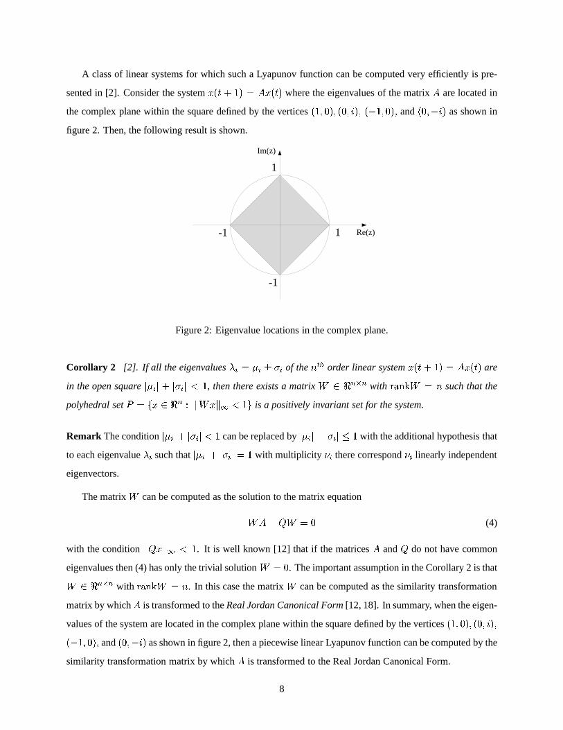
A class of linear systems for which such a Lyapunov function can be computed very efficiently is pre-
sented in [2]. Consider the systemx(t + 1) = Ax(t) where the eigenvalues of the matrixA are located in
the complex plane within the square defined by the vertices(1; 0); (0; i); (1; 0); and(0;i) as shown in
figure 2. Then, the following result is shown.
1
1
-1
-1
Re(z)
Im(z)
Figure 2: Eigenvalue locations in the complex plane.
Corollary 2 [2]. If all the eigenvaluesi = i i of thenth order linear systemx(t+ 1) = Ax(t) are
in the open squarejij + jij < 1, then there exists a matrixW 2 <nn with rankW = n such that the
polyhedral setP = fx 2 <n : kWxk1 < 1g is a positively invariant set for the system.
Remark The conditionjij+ jij < 1 can be replaced byjij+ jij 1 with the additional hypothesis that
to each eigenvaluei such thatjij+ jij = 1 with multiplicity i there correspondi linearly independent
eigenvectors.
The matrixW can be computed as the solution to the matrix equation
WAQW = 0 (4)
with the conditionkQxk1 < 1. It is well known [12] that if the matricesA andQ do not have common
eigenvalues then (4) has only the trivial solutionW = 0. The important assumption in the Corollary 2 is that
W 2 <nn with rankW = n. In this case the matrixW can be computed as the similarity transformation
matrix by whichA is transformed to theReal Jordan Canonical Form[12, 18]. In summary, when the eigen-
values of the system are located in the complex plane within the square defined by the vertices(1; 0); (0; i);
(1; 0); and(0;i) as shown in figure 2, then a piecewise linear Lyapunov function can be computed by the
similarity transformation matrix by whichA is transformed to the Real Jordan Canonical Form.
8

nIn our stability analysis for switched linear systems, it is not necessary for the individual invariant poly-
hedral sets to be centrally symmetric. Positively invariant polyhedral sets for stable discrete-time systems can
be determined usingcomputer generated Lyapunov functions[8]. The class of computer generated Lyapunov
functions has been used for stability analysis of nonlinear systems in [8, 9, 23, 26]. The main idea is to con-
struct a Lyapunov function that guarantees the stability of a set of matrices that is determined by applying
Euler’s discretization method to a system of nonlinear differential equations.
Our approach here is to use a computer generated Lyapunov function for each individual subsystem. Con-
sider the matrixA 2 <nn and letP0 <n be a bounded polyhedral region of the origin. We denote the
convex hull ofP by conv(P ). Following [8] we define
Pk = conv
1[i=0
AiPk1
!(5)
and
P =1[i=0
Pi: (6)
The following results may be found [8]: First, the matrixA is stable if and only ifP is bounded. Second, if
A is stable then each setPk can be computed byPk1 using finitely many iterations. Furthermore, it is shown
in [9] that if there exists constantK 2 < such that the eigenvalues ofA satisfy the conditionjij K < 1,
then the setP is finitely computable. In this case the setP is polyhedral as the convex hull of finitely
many points. Furthermore,P is a positively invariant polyhedral set of the system. Then, a piecewise linear
Lyapunov function can be defined as the Lyapunov function induced by the setP .
4 Stabilizing Switching Sequences
In this section, we present an approach based on multiple Lyapunov functions for the stability analysis of the
switched system (1). The main contribution is an efficient characterization of a class of switching laws of
the form (2) which guarantee the stability of the system.
We assume that each individual subsystem admits a positively invariant polyhedral set that contains the
origin which is described by
Pq = fx 2 <n : W qx < 1g
whereW q 2 <mqn and1 = [1; : : : ; 1]T 2 <n. In view of the above results, such a polyhedral set can be
computed if there exists constantK 2 < such that the eigenvalues ofA satisfy the conditionjij K < 1.
9

We denote the rows of the matrixW q bywqi 2 <n; i = 1; : : : ;mq. The Lyapunov function induced by the
setPq can be described by
Vq(x) = max1imq
hx;wqi i:
Note that ifPq is centrally symmetric then there existsW q 2 <nn and the corresponding Lyapunov function
can be written asVq(x) = kW qxk1.
We consider a classSd of switching sequences of the form
s = (q0; t0); (q1; t1); : : : ; (qj ; tj); : : : ; x(t0) = x0:
The meaning of the above notation is that the subsystemqj is becoming active at timetj . It is assumed that
if s is finite with cardinalityj + 1 thentj+1 = 1 so we can study the stability properties of the switched
system. Furthermore, it is assumed thatqj 6= qj+1 which means that the switching sequences contains only
time instants when a switching occurs. Such a sequence can be generated by the switching lawqj(tj +1) =
Æ(qj1(tj); x(tj)); j = 1; 2; : : :.
Consider the multiple Lyapunov function defined byV [x(t)] = Vqj [x(t)]; tj < t tj+1 then by the
definition ofVqj we have that for everyt > t0; t 2 Z+ DV (x) = V [x(t + 1)] V [x(t)] 0. Note that
the switched system for a fixed switching sequences can be viewed as a time-varying system. SinceV (x)
is positive definite and radially unbounded, andDV negative semidefinite, the system is stable in the sense
of Lyapunov (see for example [1]) and the following proposition can be stated.
Proposition 1 Consider a switching sequences 2 S. If Vqj [x(tj + 1)] Vqj1 [x(tj)]; j = 1; 2; : : :, then
the switched systemx(t+ 1) = Aqx(t) is stable in the sense of Lyapunov.
Remark If the conditionVqj [x(tj +1)] < Vqj1 [x(tj)] is used in the previous proposition, then the origin is
asymptotically stable for the switched system.
A multiple Lyapunov function composed by piecewise linear Lyapunov functions of the individual sub-
systems offers a significant advantage. It allows the characterization of the switching sequences that satisfy
the condition of Proposition 1 by computing a conic partition of the state space. First, we briefly describe the
necessary notions and notation from convex analysis in order to construct the conic partition.
Given a polytopeP 2 <n, then a face of dimensionk is denoted askfaceF . The hyperplane that
corresponds to akfaceF is defined by the affine hull ofF and is denoted by aff(F ). Each(n 1)face
corresponds to a hyperplane that is defined by
aff(Fi) = fx 2 <n : hx;wii = 1g
10

wherewi 2 <n is the corresponding gradient vector. The set of vertices ofF can be found as vert(F ) =
vert(P )\aff(F ) where vert(P ) is the set of vertices of the polytopeP . Finally, we denote the cone generated
by the vertices ofF by cone(F ).
Consider a pair of subsystems with matricesAq1 andAq2 . We want to compute the regionq2q1
= fx 2
<n : Vq2(x) Vq1(x)g. Consider the facesF q1i1
andF q2i2
of the polytopesPq1 andPq2 respectively and
assume thatC = cone(F q1i1) \ cone(F q2
i2) 6= ;. Next, we define the halfspaceHq2
q1= fx 2 <n : hx;wq2
i2
wq1i1i 0g and the set = C\Hq2
q1. It is shown in the following lemma that the multiple Lyapunov function
defined in Proposition 1 is decreasing if the system switches fromq1 to q2 while x 2 .
Lemma 1 For everyx 2 we have thatVq2(x) Vq1(x).
Proof For everyx 2 C the Lyapunov functions for the subsystems are given byVq1(x) = hx;wq1i1i and
Vq2(x) = hx;wq2i2i respectively. Ifx 2 we have thathx;wq2
i2 w
q1i1i 0 sincex 2 Hq2
q1, and therefore
Vq2(x) Vq1(x). 2
Since0 2 Hq2q1
, the set is clearly a polyhedral cone as the intersection of cones with a common apex
(x = 0) as shown in figure 3.
H
x
x
1
2
q2
q1
Fq
1i1
Pq1
Pq2
Ω
Fq
2i2
Figure 3: The conic partition of the state space.
The setq2q1
can be computed as the union of polyhedral cones by repeating the above procedure for all
the pairs(F q1i1; F
q2i2) of (n 1)faces of the polytopeP as shown in the following algorithm.
Algorithm for the computation of q2q1
11

INPUT:W q1 ;W q2 ;
for i1 = 1; : : : ;mq1
for i2 = 1; : : : ;mq2
C = cone(F q1i1) \ cone(F q2
i2);
if C 6= ; then
Hq2q1
= fx 2 <n : hx;wq2i2 w
q1i1i 0g
= C \Hq2q1;
q2q1
= q2q1[ ;
end
end
end
The above procedure can be repeated for every pair of subsystems to identify a class of stabilizing switch-
ing signals for the switched linear system. The class of switching sequences is characterized by the following
result.
Theorem 2 Consider the class of switching sequences~Sd Sd defined by
qj(tj + 1) = Æ(qj1(tj); x(tj))
x(tj) 2 qjqj1 6= ;
for j = 1; 2; : : :. The switched linear systemx(t+ 1) = Aqx(t) is stable in the sense of Lyapunov for every
switching sequences 2 ~Sd.
Proof By induction, we have that ifs = (q0; t0) then the system is stable sinceAq0 is stable. Assume that the
switched system is stable fors = (q0; t0); (q1; t1); : : : ; (qj1; tj1) and consider the switching sequences0 =
(q0; t0); (q1; t1); : : : ; (qj1; tj1); (qj ; tj). Sincex(tj) 2 qjqj1 , we have thatVqj [x(tj)] Vqj1 [x(tj)].
Therefore, the multiple Lyapunov function defined byV [x(t)] = Vqj [x(t)]; tj < t tj+1 is decreasing for
everyt and the system is stable in the sense of Lyapunov. 2
We have presented a methodology for the partition of the state space into conic regions that are used to
characterize a class of stabilizing switching sequences. The following example illustrates the approach.
12
ExampleConsider the switched discrete-time linear systemx(t+ 1) = Aqx(t); q 2 f1; 2g where
A1 =
264 1:7 4
0:8 1:5
375 andA2 =
264 0:95 1:5
0:75 0:55
375 :
The system with matrixA1 has two complex conjugate eigenvalues1;2 = 0:1 j0:8 and satisfies the
conditions of Corollary 2. Using the similarity transformation
W 1 =
264 1 2
0 1
375 :
the real Jordan canonical form is given by
Q1 = W 1A1(W1)1 =
264 0:1 0:8
0:8 0:1
375 :
We have that
kQ1k1 = max1in
nXj=1
jqijj = 0:9 < 1
and therefore by Theorem 1,V1(x) = kW 1xk1 is a Lyapunov function for the system. Furthermore, the set
P1 = fx 2 <2 : kW 1xk1 1g
shown in figure 4 is a positively invariant polyhedral set. The matrixA2 has two complex conjugate eigen-
values1;2 = 0:2 j0:75. A positively invariant polyhedral setP2 is described by the Lyapunov function
V2 = kW 2xk1 where
W 2 =
264 1 2
1 0
375 :
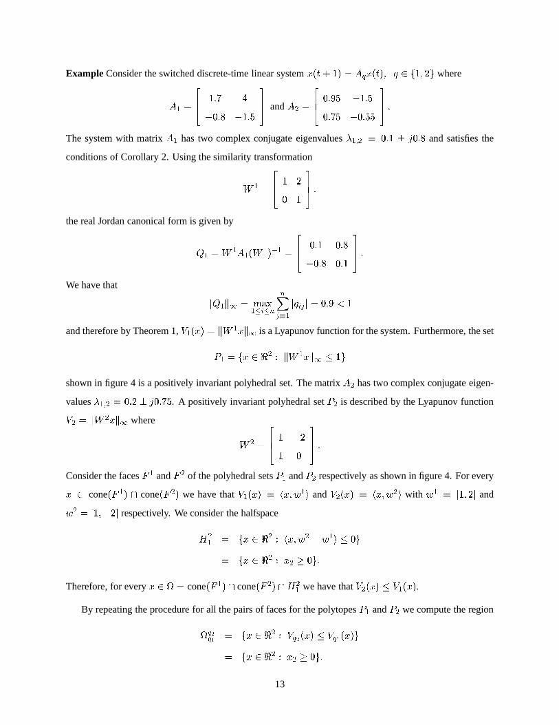
Consider the facesF 1 andF 2 of the polyhedral setsP1 andP2 respectively as shown in figure 4. For every
x 2 cone(F 1) \ cone(F 2) we have thatV1(x) = hx;w1i andV2(x) = hx;w2i with w1 = [1; 2] and
w2 = [1;2] respectively. We consider the halfspace
H21 = fx 2 <2 : hx;w2 w1i 0g
= fx 2 <2 : x2 0g:
Therefore, for everyx 2 = cone(F 1) \ cone(F 2) \H21 we have thatV2(x) V1(x).
By repeating the procedure for all the pairs of faces for the polytopesP1 andP2 we compute the region
q2q1
= fx 2 <2 : Vq2(x) Vq1(x)g
= fx 2 <2 : x2 0g:
13

−4 −3 −2 −1 0 1 2 3 4−2
−1.5
−1
−0.5
0
0.5
1
1.5
2
x
x
1
2 F1
P1
P2
F2
Ω
Figure 4: The region.
Similarly we have that
q1q2
= fx 2 <2 : Vq1(x) Vq2(x)g
= fx 2 <2 : x2 0g:
Therefore, for any switching sequences given by the switching law
q2(t+ 1) = Æ(q1(t); x(t))
x(t) 2 q2q1
and
q1(t+ 1) = Æ(q2(t); x(t))
x(t) 2 q1q2
the switched system is stable. A stable trajectory is shown in figure 5.
The characterization of the stabilizing switching sequences is based on sufficient conditions. Therefore,
for a switching sequences that does not satisfy the formulated conditions, the switched system is not nec-
essarily unstable. However, the switched system of the example can generate unstable trajectories as shown
in figure 6. A switching law leads to unstable trajectories if the corresponding switching sequence is infinite
and there exists a Lyapunov functions that increases at every switching instant. 2
14

x1
x2
−6 −4 −2 0 2 4 6−6
−4
−2
0
2
4
6
Figure 5: A stable trajectory for the discrete-time switched system.
5 Continuous-time Switched Linear Systems
In this section, a characterization of stabilizing switching sequences for continuous-time switched linear sys-
tems is presented. The set of stabilizing switching sequences is characterized by computing a conic partition
of the state space similarly to the discrete-time case.
We consider the switched linear system
_x(t) = Aqx(t); q 2 Q f1; : : : ; Ng (7)
wherex(t) 2 <n andAq 2 <nn. The switching law is described by
q(t+) = Æ(q(t); x(t)): (8)
wheret+ = lim!t; >t . The problem is to identify classes of switching signals generated by (8) for which
the system (7) is stable. Note that in the following it is assumed that only finitely many switchings can occur
in a finite time interval (non-Zeno behavior).
5.1 Background Material
In order to study the stability properties of the switched linear system (7), we assume that each individual
subsystem admits a piecewise linear Lyapunov function induced by a positively invariant polyhedral set.
15

−0.5 0 0.5 1 1.5 2 2.5 3
x 10129
−1
−0.8
−0.6
−0.4
−0.2
0
0.2
0.4
0.6
0.8
1x 10
129
x1
x2
Figure 6: An unstable trajectory of the discrete-time switched system.
Next, we summarize some results from [15] for the computation of piecewise linear Lyapunov functions for
a class of continuous-time linear systems.
Consider the continuous-time linear system
_x(t) = Ax(t); q 2 Q f1; : : : ; Ng (9)
wherex(t) 2 <n andA 2 <nn.
Similarly to the discrete-time case, there exists a class of continuous linear systems for which a positively
invariant polyhedral set can be computed very efficiently. If the eigenvaluesi of the system (9) satisfy the
condition jImfigj < jRefigj as shown in figure 7 then a Lyapunov functionV (x) = kWxk1 can be
constructed using a similarity transformation [15].
The use of piecewise linear Lyapunov functions for the stability of linear systems is based on the fol-
lowing result [13]. Assume that there exists a functionV (x) such thatV is positive definite and radially
unbounded, and theupper right Dini derivative[6] of V satisfies the condition
DV = limt!0
supV [x(t+t)] V [x(t)]
t 0:
Then, the equilibriumx = 0 is stable in the sense of Lyapunov.
The conditions forV (x) = kWxk1 to be a Lyapunov function for the system (9) can be stated using the
logarithmic norm induced by the infinity norm. The logarithmic norm1 of a matrixQ 2 <nn is defined
16

1
-1
-1
Re(z)
Im(z)
Figure 7: Eigenvalue locations in the complex plane.
as [11]
1(Q) = lim!0+
kI Qk1 1
= maxifqii +
Xj=1;j 6=i
jqij jg
.
The following theorem presented in [15, 28] gives necessary and sufficient conditions forV (x) = kWxk1
to be a Lyapunov function of the system (9).
Theorem 3 [15] V (x) = kWxk1 is a Lyapunov function for the system_x = Ax(t) if and only if there
existsQ 2 <nn such thatWAQW = 0 and1(Q) < 0.
A class of linear systems for which a piecewise linear Lyapunov function can be computed very efficiently
is presented in [15] and it is described by the following corollary.
Corollary 3 [15] If all the eigenvaluesi = ii of thenth order system_x = Ax(t) satisfy the condition
jij jij, then there existsW 2 <nn with rankW = n such that the polyhedral setP = fx 2 <n :
kWxk1 < 1g is a positively invariant set for the system.
The above corollary is a consequence of the fact that the matrix equationWAQA = 0 has a solution
W with rankW = n if and only if the eigenvalues ofA are identical with the eigenvalues ofQ [12]. The
matrixW can be computed as the similarity transformation matrix by whichA is transformed to the real
Jordan canonical form similar to the discrete-time case.
17

5.2 Stabilizing Switching Sequences
In this section, we present an approach based on multiple Lyapunov functions for the stability analysis of the
switched system (7). We assume that each individual subsystem admits a piecewise linear Lyapunov function
described by the infinity norm. The main contribution is an efficient characterization of a class of switching
laws of the form (8) which guarantee the stability of the system. Similar results can be developed for more
general piecewise linear Lyapunov functions as in the discrete-time case in Section 4.
We assume that each individual subsystem admits a positively invariant polyhedral set that contains the
origin which is described by
Pq = fx 2 <n : kW qxk1 < 1g
whereW q 2 <nn. We denote the rows of the matrixW q bywqi 2 <
n; i = 1; : : : ;mq.
We consider a classSc of switching sequences of the form
s = (q0; t0); (q1; t1); : : : ; (qj ; tj); : : : ; x(t0) = x0:
wheretj 2 <n; j = 0; 1; : : :. It is assumed that the sequence of switching instantst0; t1; : : : ; tj ; : : : is di-
vergent in the sense that there are no infinitely many switchings in a finite time interval. Similarly to the
discrete-time case, it is assumed thatqj 6= qj+1. A sequences can be generated by the switching law
qj(t+j ) = Æ(qj1(tj); x(tj)); j = 1; 2; : : :.
Consider the multiple Lyapunov function defined byV [x(t)] = Vqj [x(t)]; tj < t tj+1. Then, we
have
DV = limt!0
supV [x(t+t)] V [x(t)]
t 0
for everyt 2 <n and therefore, the equilibriumx = 0 is stable in the sense of Lyapunov (see for exam-
ple [13]), and the following proposition can be stated.
Proposition 2 Consider a switching sequences 2 S. If Vqj [x(t+j )] Vqj1 [x(tj)]; j = 1; 2; : : :, then the
switched system_x = Aqx(t) is stable in the sense of Lyapunov.
A conic partition of the state space can be used to characterize a class of switching sequences that satisfy
the condition of Proposition 2. Consider a pair of subsystems with matricesAq1 andAq2 . The regionq2q1
=
fx 2 <n : Vq2(x) Vq1(x)g can be computed as a union of finitely generated cones and can be computed
by the algorithm presented in Section 4 similarly to the discrete-time case. The class of stabilizing switching
sequences is characterized by the following result.
18

Theorem 4 Consider the class of switching sequences~Sc Sc defined by
qj(t+j ) = Æ(qj1(tj); x(tj))
x(tj) 2 qjqj1 6= ;
for j = 1; 2; : : :. The switched linear system_x = Aqx(t) is stable in the sense of Lyapunov for every switch-
ing sequences 2 ~Sc.
Proof Similar to the proof of Theorem 2. 2
Example
Consider the switched continuous-time linear system
_x = Aqx(t); q 2 f1; 2g (10)
where
A1 =
264 1:7 1:8
4:5 3:7
375 andA2 =
264 0:7 1
1:6 1:7
375 :
The real Jordan canonical form can be computed by the following similarity transformations.
Q1 = W 1A1(W1)1 =
264 1 0:9
0:9 1
375
where
W 1 =
264 2 1
1 1
375
and
Q2 = W 2A2(W2)1 =
264 0:5 0:4
0:4 0:5
375
where
W 2 =
264 1 1
1 0:5
375 :
We have that1(Q1) = 0:1 < 0 and therefore,V1(x) = kW 1xk1 is a Lyapunov function for the
subsystemA1. Similarly, 1(Q2) = 0:1 < 0 andV2(x) = kW 2xk1 is a Lyapunov function for the
subsystemA2. The functionsV1 andV2 correspond to the positively invariant polyhedral setsP1 = fx 2
<2 : kW 1xk1 1g andP2 = fx 2 <2 : kW 2xk1 1g shown in figure 8.
19

−5 −4 −3 −2 −1 0 1 2 3 4 5−5
−4
−3
−2
−1
0
1
2
3
4
5
P1
P2
x1
x2
Figure 8: Positively invariant polyhedral sets.
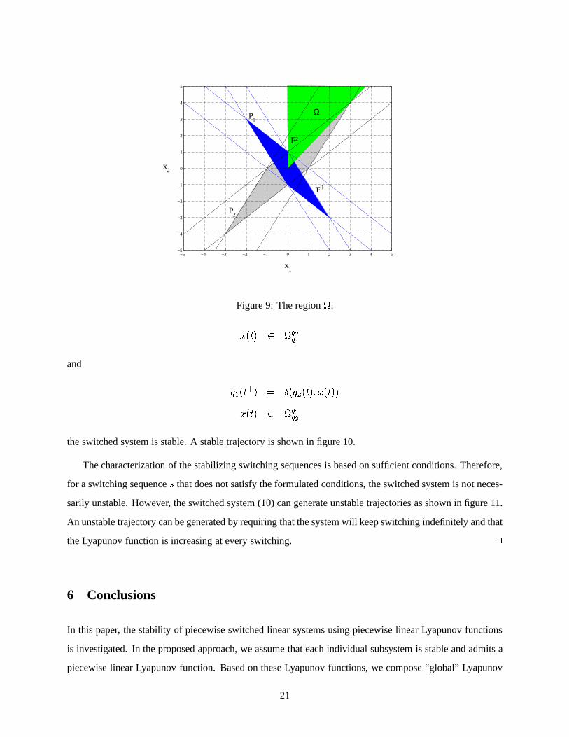
Consider the facesF 1 andF 2 shown in figure 9. For everyx 2 cone(F 1) \ cone(F 2) we have that
V1(x) = hx;w1i andV2(x) = hx;w2i with w1 = [2; 1] andw2 = [1; 1] respectively. We consider the
halfspace
H21 = fx 2 <2 : hx;w2 w1i 0g
= fx 2 <2 : x1 0g:
Therefore, for everyx 2 = cone(F 1) \ cone(F 2) \H21 we have thatV2(x) V1(x).
By repeating the procedure for all the pairs of faces for the polytopesP1 andP2 the we compute the
region
q2q1
= fx 2 <2 : Vq2(x) < Vq1(x)g
= fx 2 <2 : x1 > 0g:
Similarly we have that
q1q2
= fx 2 <2 : Vq1(x) < Vq2(x)g
= fx 2 <2 : x1 < 0g:
Therefore, for any switching sequences given by the switching law
q2(t+) = Æ(q1(t); x(t))
20
−5 −4 −3 −2 −1 0 1 2 3 4 5−5
−4
−3
−2
−1
0
1
2
3
4
5
P1
P2
x1
x2
F1
F2
Ω
Figure 9: The region.
x(t) 2 q2q1
and
q1(t+) = Æ(q2(t); x(t))
x(t) 2 q1q2
the switched system is stable. A stable trajectory is shown in figure 10.
The characterization of the stabilizing switching sequences is based on sufficient conditions. Therefore,
for a switching sequences that does not satisfy the formulated conditions, the switched system is not neces-
sarily unstable. However, the switched system (10) can generate unstable trajectories as shown in figure 11.
An unstable trajectory can be generated by requiring that the system will keep switching indefinitely and that
the Lyapunov function is increasing at every switching. 2
6 Conclusions
In this paper, the stability of piecewise switched linear systems using piecewise linear Lyapunov functions
is investigated. In the proposed approach, we assume that each individual subsystem is stable and admits a
piecewise linear Lyapunov function. Based on these Lyapunov functions, we compose “global” Lyapunov
21

−5 −4 −3 −2 −1 0 1 2−1
0
1
2
3
4
5
6
Subsystem 1
Subsystem 2
1x
2x
Figure 10: A stable trajectory for the continuous-time switched system.
functions that guarantee stability of the switched linear system. These multiple Lyapunov functions corre-
spond to conic partitions of the state space which are efficiently computed using the developed algorithms.
The main advantage of the approach is that the methodology for computing switching laws that guarantee
stability is based on the parameters of the system and so, trajectories for particular initial conditions do not
need to be calculated. Therefore, the proposed approach can be used very efficiently to investigate the sta-
bility properties of practical hybrid systems.
AcknowledgementsThe partial financial support of the National Science Foundation (EC99-12458) and the
Army Research Office (DAAG55-98-1-0199) is gratefully acknowledged.
References
[1] P. Antsaklis and A. Michel.Linear Systems. McGraw-Hill, 1997.
[2] G. Bitsoris. Positively invariant polyhedral sets of discrete-time linear systems.International Journal
of Control, 47(6):1713–1726, 1988.
[3] G. Bitsoris and E. Gravalou. Comparison principle, positive invariance and constrained regulation of
nonlinear systems.Automatica, 31(2):217–222, 1995.
22

0 50 100 150 200 250−600
−500
−400
−300
−200
−100
0
100
200
300
400
1x
2x
Figure 11: An unstable trajectory of the continuous-time switched system.
[4] G. Bitsoris and M. Vassilaki. Constrained regulation of linear systems.Automatica, 31(2):223–227,
1995.
[5] F. Blanchini. Nonquadratic Lyapunov functions for robust control.Automatica, 31(3):451–461, 1995.
[6] F. Blanchini. Set invariance in control.Automatica, 35(11):1747–1767, 1999.
[7] M. Branicky. Multiple Lyapunov functions and other analysis tools for switched and hybrid systems.
IEEE Transactions on Automatic Control, 43(4):475–482, 1998.
[8] R. Brayton and C. Tong. Stability of dynamical systems: A constructive approach.IEEE Transactions
on Circuits and Systems, CAS-26(4):224–234, 1979.
[9] R. Brayton and C. Tong. Constructive stability and asymptotic stability of dynamical systems.IEEE
Transactions on Circuits and Systems, CAS-27(11):1121–1130, 1980.
[10] R. DeCarlo, M. Branicky, S. Pettersson, and B. Lennartson. Perspectives and results on the stability
and stabilizability of hybrid systems.Proceedings of IEEE, 88(7):1069–1082, July 2000.
[11] V. Desoer and H. Haneda. The measure of a matrix as a tool to analyze computer algorithms for circuit
analysis.IEEE Transactions on Circuit Theory, 19(5):480–486, 1972.
[12] F. Gantmacher.Matrix Theory. Chelsea, 1959.
23
[13] W. Hahn.Stability of Motion. Springer-Verlag, 1967.
[14] M. Johansson and A. Rantzer. Computation of piecewise quadratic Lyapunov functions for hybrid sys-
tems.IEEE Transactions on Automatic Control, 43(4):555–559, 1998.
[15] H. Kiendl, J. Adamy, and P. Stelzner. Vector norms as Lyapunov functions for linear systems.IEEE
Transactions on Automatic Control, 37(6):839–842, 1992.
[16] X. Koutsoukos. Analysis and Design of Piecewise Linear Hybrid Dynamical Systems. PhD thesis,
Department of Electrical Engineering, University of Notre Dame, Notre Dame, IN, 2000.
[17] X. Koutsoukos and P. Antsaklis. Stabilizing supervisory control of hybrid systems based on piecewise
linear Lyapunov functions. InProceedings of the 8th IEEE Mediterranean Conference on Control and
Automation, Rio, Greece, July 2000.
[18] P. Lancaster and M. Tismenetsky.The Theory of Matrices. Academic Press, 1985.
[19] D. Liberzon and A. Morse. Basic problems in stability and design of switched systems.IEEE Control
Systems Magazine, 19(5):59–70, October 1999.
[20] K. Loskot, A. Polanski, and R. Rudnicki. Further comments on Vector norms as Lyapunov functions
for linear systems.IEEE Transactions on Automatic Control, 43(2):289–291, 1998.
[21] N. H. McCLamroch and I. Kolmanovsky. Performance benefits of hybrid control design for linear and
nonlinear systems.Proceedings of IEEE, 88(7):1083–1096, July 2000.
[22] A. Michel. Recent trends in the stability analysis of hybrid dynamical systems.IEEE Transactions on
Circuits and Systems I, 46(1):120–134, 1999.
[23] A. Michel, B. Nam, and V. Vittal. Computer generated Lyapunov functions for interconnected sys-
tems: Improved results with applications to power systems.IEEE Transactions on Circuits and Sys-
tems, CAS-31(2):189–198, 1984.
[24] D. Mitra and H. So. Existence conditions forl1 Lyapunov functions for a class of nonautonomous
systems.IEEE Transactions on Circuit Theory, CT-19(6):594–598, 1972.
[25] A. Molchanov and Y. Pyatnitskiy. Criteria of asymptotic stability of differential and difference inclu-
sions encountered in control theory.Systems & Control Letters, 13:59–64, 1989.
24

[26] Y. Ohta, H. Imanishi, L. Gong, and H. Haneda. Computer generated Lyapunov functions for a class of
nonlinear systems.IEEE Transactions on Circuits and Systems-I: Fundamental Theory and Applica-
tions, 40(5):428–433, 1993.
[27] S. Pettersson and B. Lennartson. Stability and robustness of hybrid systems. InProceedings of the 35th
IEEE Conference on Decision and Control, pages 1202–1207, Kobe, Japan, December 1996.
[28] A. Polanski. On infinity norms as Lyapunov functions for linear systems.IEEE Transactions on Auto-
matic Control, 40(7):1270–1273, 1995.
[29] A. Polanski. Lyapunov function construction by linear programming.IEEE Transactions on Automatic
Control, 42(7):1013–1016, 1997.
[30] H. Rosenbrock. A Liapunov function for some naturally-occuring linear homogeneous time-dependent
equations.Automatica, 1(2/3):97–109, 1963.
[31] H. Rosenbrock. A Liapunov function with application to some nonlinear physical systems.Automatica,
1(1):31–53, 1963.
[32] S. Weissenberger. Piecewise-quadratic and piecewise-linear Lyapunov functions for discontinuous sys-
tems.International Journal of Control, 10(2):171–180, 1969.
[33] S. Weissenberger. Stability of regions for large scale systems.Automatica, 9:653–663, 1973.
[34] X. Xu and P. Antsaklis. Stabilization of second-order LTI switched systems.Internation Journal of
Control, 73(14):1261–1279, 2000.
[35] H. Ye, A. Michel, and L. Hou. Stability theory for hybrid dynamical systems.IEEE Transactions on
Automatic Control, 43(4):461–474, 1998.
[36] C. Yfoulis, A. Muir, P. Wellstead, and N. Pettit. Stabilization of orthogonal piecewise linear systems:
Robustness analysis and design. In F. Vaandrager and J. van Schuppen, editors,Hybrid Systems—
Computation and Control, (HSCC’99), volume 1569 ofLecture Notes in Computer Science, pages 256–
270. Springer-Verlag, 1999.
25