design of flexible soft output mimo detector for...
TRANSCRIPT

Design of Flexible Soft Output MIMO Detector for
Cooperative MIMO
Milos Jorgovanovic
Electrical Engineering and Computer SciencesUniversity of California at Berkeley
Technical Report No. UCB/EECS-2013-170
http://www.eecs.berkeley.edu/Pubs/TechRpts/2013/EECS-2013-170.html
October 15, 2013

Copyright © 2013, by the author(s).All rights reserved.
Permission to make digital or hard copies of all or part of this work forpersonal or classroom use is granted without fee provided that copies arenot made or distributed for profit or commercial advantage and that copiesbear this notice and the full citation on the first page. To copy otherwise, torepublish, to post on servers or to redistribute to lists, requires prior specificpermission.

Design of Flexible Soft Output MIMO Detector for Cooperative MIMO
System
by Milos Jorgovanovic
Research Project
Submitted to the Department of Electrical Engineering and Computer Sciences, University of Cali-
fornia at Berkeley, in partial satisfaction of the requirements for the degree of Master of Science,
Plan II.
Approval for the Report and Comprehensive Examination:
Committee:
Professor Borivoje Nikolic
Research Advisor
Date
* * * * * *
Professor David Tse
Second Reader
Date

Design of Flexible Soft Output MIMO Detector for
Cooperative MIMO System
Milos Jorgovanovic

Ani, Emiliji, Nebojsi
1
Contents
1 Introduction 1
1.1 Motivation . . . . . . . . . . . . . . . . . . . . . . . . . . . . . . . . . . . . . . . . . 1
1.2 MIMO Detection . . . . . . . . . . . . . . . . . . . . . . . . . . . . . . . . . . . . . . 3
1.3 Thesis Outline . . . . . . . . . . . . . . . . . . . . . . . . . . . . . . . . . . . . . . . 4
2 Cooperative MIMO System 5
2.1 MIMO System with Co-located Antennas . . . . . . . . . . . . . . . . . . . . . . . . 5
2.2 Cooperation Between Terminals . . . . . . . . . . . . . . . . . . . . . . . . . . . . . . 6
2.3 Space-Time Coding . . . . . . . . . . . . . . . . . . . . . . . . . . . . . . . . . . . . . 9
2.4 Joint LDPC Decoding . . . . . . . . . . . . . . . . . . . . . . . . . . . . . . . . . . . 10
3 Soft Output MIMO Detector for DBLAST 13
3.1 Linear Detectors . . . . . . . . . . . . . . . . . . . . . . . . . . . . . . . . . . . . . . 14
3.1.1 MMSE Detector . . . . . . . . . . . . . . . . . . . . . . . . . . . . . . . . . . 15
3.1.2 MMSE-SIC Detector . . . . . . . . . . . . . . . . . . . . . . . . . . . . . . . . 16
3.2 Square Root Algorithm for MMSE-SIC . . . . . . . . . . . . . . . . . . . . . . . . . . 18
3.3 Algorithm Extension for Soft Bit Output Generation . . . . . . . . . . . . . . . . . . 23
3.4 Soft Bit Output Generation . . . . . . . . . . . . . . . . . . . . . . . . . . . . . . . . 26
3.5 2x2 MIMO Performance of the Proposed Algorithm . . . . . . . . . . . . . . . . . . 31
4 Hardware Implementation 34
4.1 Implementation of the Systolic Array . . . . . . . . . . . . . . . . . . . . . . . . . . . 36
4.1.1 Nulling a Single Element in a Row . . . . . . . . . . . . . . . . . . . . . . . . 37
4.1.2 CORDIC Implementation . . . . . . . . . . . . . . . . . . . . . . . . . . . . . 40
4.1.3 Systolic Array for Nulling a Single Element . . . . . . . . . . . . . . . . . . . 43
4.1.4 Nulling the Row of the Matrix . . . . . . . . . . . . . . . . . . . . . . . . . . 46
i

Flexible Soft Output MIMO Detector Milos Jorgovanovic
4.2 MMSE-SIC Preprocessing — Coefficient Calculation . . . . . . . . . . . . . . . . . . 47
4.2.1 Matrix Update for Square-root Algorithm . . . . . . . . . . . . . . . . . . . . 48
4.2.2 Final Remarks on the Implementation of Preprocessing Unit . . . . . . . . . 49
4.3 Critical Path . . . . . . . . . . . . . . . . . . . . . . . . . . . . . . . . . . . . . . . . 49
4.3.1 Modulator . . . . . . . . . . . . . . . . . . . . . . . . . . . . . . . . . . . . . . 52
4.3.2 SIC . . . . . . . . . . . . . . . . . . . . . . . . . . . . . . . . . . . . . . . . . 52
4.3.3 MMSE-SIC Filter . . . . . . . . . . . . . . . . . . . . . . . . . . . . . . . . . 53
4.3.4 Soft Bit Demodulator . . . . . . . . . . . . . . . . . . . . . . . . . . . . . . . 53
4.4 Interface . . . . . . . . . . . . . . . . . . . . . . . . . . . . . . . . . . . . . . . . . . . 55
4.5 Speed Performance and Resource Utilization . . . . . . . . . . . . . . . . . . . . . . 56
5 Conclusion 58
ii
List of Figures
1.1 a) MIMO system; b) Cooperative MIMO system. . . . . . . . . . . . . . . . . . . . . 2
2.1 Simple block diagram of the 2x2 MIMO channel. . . . . . . . . . . . . . . . . . . . . 6
2.2 2x2 MIMO system with channel encoding and modulation. . . . . . . . . . . . . . . 6
2.3 Cooperative MIMO system subframe structure. . . . . . . . . . . . . . . . . . . . . . 7
2.4 Quantize and map scheme applied to the cooperative MIMO scenario. . . . . . . . . 8
2.5 Simplified block diagram of the source-relay-destination system. . . . . . . . . . . . . 9
2.6 BLAST space-time coding schemes for MIMO. . . . . . . . . . . . . . . . . . . . . . 10
2.7 Factor graphs capturing the relations between sources and relays messages for different
space-time coding schemes: (a) VBLAST, (b) DBLAST. . . . . . . . . . . . . . . . . 11
2.8 Factor graph for joint LDPC decoding at the destination. . . . . . . . . . . . . . . . 12
3.1 DBLAST space-time coding. . . . . . . . . . . . . . . . . . . . . . . . . . . . . . . . 14
3.2 Block Diagram of MMSE Detection for DBLAST. . . . . . . . . . . . . . . . . . . . 16
3.3 Block Diagram of MMSE-SIC Detection for DBLAST. . . . . . . . . . . . . . . . . . 18
3.4 Performance of the max-log soft demodulator vs. ideal soft demodulator, point-to-
point AWGN channel with rate 0.5 LDPC coding. . . . . . . . . . . . . . . . . . . . 28
3.5 16-QAM constellation for LTE standard. . . . . . . . . . . . . . . . . . . . . . . . . . 28
3.6 16-QAM constellation divided into detection regions for each bit. . . . . . . . . . . . 29
3.7 Simplification for distance calculation in (3.57) for bit 2 of 16-QAM conatellation. . 30
3.8 BER curves for 2x2 MIMO with DBLAST and per symbol interleaving — ideal
MMSE-SIC and proposed design using square-root algorithm and max-log soft de-
modulator. . . . . . . . . . . . . . . . . . . . . . . . . . . . . . . . . . . . . . . . . . 33
4.1 Block diagram of the implemented MMSE-SIC MIMO detector. . . . . . . . . . . . . 35
4.2 Achieving rotation through ξ by using minirotations through the special angles ±ξυ. 41
iii

Flexible Soft Output MIMO Detector Milos Jorgovanovic
4.3 Rotation of a vector through angle ξ using CORDIC algorithm. . . . . . . . . . . . . 41
4.4 Achieving rotation through ξ using minirotations through the special angles ±ξυ,
using one correction gain. . . . . . . . . . . . . . . . . . . . . . . . . . . . . . . . . . 41
4.5 Pipeline CORDIC circuit. . . . . . . . . . . . . . . . . . . . . . . . . . . . . . . . . . 43
4.6 Uncoded MMSE-SIC detector performance versus number of stages in CORDIC. . . 44
4.7 CORDIC Super Cell block. . . . . . . . . . . . . . . . . . . . . . . . . . . . . . . . . 45
4.8 Block diagram of the Null Row block. . . . . . . . . . . . . . . . . . . . . . . . . . . 47
4.9 Simplified block diagram of the Preprocessing unit. . . . . . . . . . . . . . . . . . . . 48
4.10 Block diagram of the Mtrx Update unit. . . . . . . . . . . . . . . . . . . . . . . . . . 50
4.11 Screenshot of the Preprocessing unit design in Simulink . . . . . . . . . . . . . . . . 51
4.12 Screenshot of the Modulator unit design in Simulink. . . . . . . . . . . . . . . . . . . 52
4.13 Block diagram of the interference cancellation unit. . . . . . . . . . . . . . . . . . . . 53
4.14 Block diagram of the MMSE-SIC filter block. . . . . . . . . . . . . . . . . . . . . . . 54
4.15 Block diagram of the soft demodulator unit. . . . . . . . . . . . . . . . . . . . . . . . 54
4.16 Interface of the designed MIMO detector. . . . . . . . . . . . . . . . . . . . . . . . . 55
iv

Chapter 1
Introduction
1.1 Motivation
Next generation wireless communication networks aim to achieve higher data throughput and im-
proved coverage. Because of the regulatory limits on frequency bands and transmit power, any future
data rate increase needs to come from using other degrees of freedom. Exploiting space as a degree
of freedom by using a Multiple-Input Multiple-Output (MIMO) concept, Figure 1.1a, has enabled
dramatic increase in the efficiency of wireless communications in the past decade. Some examples of
wireless standards that successfully deployed MIMO are 801.11n for personal area network and the
new LTE standard for cellular (4G). MIMO does have potential for achieving large data rates, but
it also has few drawbacks. It has been shown that antennas need to be separated by at least half the
carrier wavelength to provide independent fading [5], [3]. In todays cellular systems this distance is
of the order of 5-10cm and is eventually limiting the number of antennas that can be mounted on
the mobile device. Another issue is the power consumption of the multi-antenna transceiver and the
fundamental limit on scaling of the battery capacity.
Increase in throughputs also requires increase in the density of the deployed infrastructure (base
stations and femto-cells), which increases the amount of interference. Finally, the infrastructure
becomes irregular and is being deployed ad-hoc (in the form of femto-cells). One key challenge in the
future wireless standards is how to constructively exploit interference in a dense, irregularly deployed
network, while keeping power consumption within given constraints. Another challenge is how to use
nearby idle terminals to help transmission. A number of theoretical concepts have emerged in the
past few years that show that cooperation between terminals can significantly increase the capacity
1

Flexible Soft Output MIMO Detector Milos Jorgovanovic
Figure 1.1: a) MIMO system; b) Cooperative MIMO system.
of the whole network [8], [13]. Simultaneously, advances in technology are enabling implementation
of the higher complexity wireless systems required for this cooperation and their deployment is
planned in the next wireless cellular standards LTE Advanced (5G) and beyond.
The motivation for this work is a step towards the practical demonstration of a wireless system
that exploits cooperation between terminals. The simplest configuration of such a system is presented
on Figure 1.1b and is referred to as a cooperative MIMO system. Compared to the standard MIMO
system from Figure 1.1a, the system we consider has two transmit terminals with one antenna each.
One of them is the original transmitter that has certain data stream to be sent and will be referred
to as the source. The second one, referred to as the relay, represents the half-duplex transceiver
that listens to the sources transmission and forwards part of that stream further to the destination.
Both transmit terminals have only one antenna, which simplifies the hardware design and reduces
the power consumption. In general, there may be more than one relay but the complexity of these
terminals is still less than the complexity of the single multi-antenna transmitter from Figure 1.1a.
Recently, it has been shown that even this simple case of cooperation can achieve significant
multiplexing gain [11]. When the source and the relay are very close to each other compared to the
distance from the destination, multiplexing gain approaches that of the regular 2x2 MIMO system. A
practical coding and signaling scheme to achieve the gain predicted in [11] has been explained in [12]
and the same paper gives overview of some basic specifications for the cooperative MIMO system
from Figure 1.1b. Space-time coding scheme is Diagonal Bell labs LAyered Space Time (DBLAST),
due to the latency of the signal processing at the relay. It means that the relay transmits its
information on the sources message with one message frame delay, when source is already sending
the next message. This further implies use of successive interference cancellation (SIC) type of
receiver at the destination, since transmit streams are now made independent. Optimal cooperative
communication scheme also requires specialized techniques for channel coding. These are developed
in [12] using LDPC codes and iterative decoding algorithms that require soft bit estimates of the
2

Flexible Soft Output MIMO Detector Milos Jorgovanovic
priors. These specifications, as well as the cooperation strategy, are presented in more detail in
Chapter 2.
1.2 MIMO Detection
MIMO detector is one of the central and most complex blocks of the MIMO receiver. The basic idea
behind MIMO detection is to decouple the transmitted streams at the receiver, after passing through
a MIMO channel. There are many algorithms that deal with the problem of MIMO detection, but
most of them can be categorized according to the type of signal processing either as linear or tree-
search. Linear algorithms include linear processing on the received signal (by multiplying it with
the certain matrix) [3], [6], [19]. Tree-search algorithms deploy some sort of the search algorithm on
the transmit symbol space [18], [7]. Their performance and complexity in general depends on the
level of the search, but they are typically much more complex than linear algorithms and provide
better performance.
The main constraint that a specific cooperation scheme described in [12] imposes on the MIMO
detector design, is the soft bit estimates generation. For tree-search algorithms this proves to be a
very complex task that either increases the total complexity beyond the available hardware resources,
or sacrifices performance by introducing some sort of approximation. Linear detection algorithms
are much easier to extend to include the soft bit estimates generation and are typically used for soft
bit output MIMO receivers.
The linear detection scheme that has been proven to achieve the capacity of the MIMO channel
[3] is the Minimum Mean Square Error SIC (MMSE-SIC) architecture. It is perfectly suited for
DBLAST space-time coding and SIC type of receiver. The main challenge of implementing this
architecture is calculation of the MMSE-SIC matrix used for linear processing of the received signal.
In general, it requires nt matrix inversions, where nt is the number of transmit antennas. This
issue has been addressed in number of papers that suggest alternative algorithms for calculation of
MMSE-SIC matrix without using matrix inversions [9], [19], [17]. These papers however describe
implementation of the MIMO detection algorithm for Vertical BLAST (VBLAST) space-time coding
and hard bit outputs.
In this work, few novel changes of the square-root algorithm proposed by Hassibi in [9] are
introduced. First, we take into account the DBLAST space-time strategy instead of VBLAST and
show how square-root algorithm simplifies in this case. We also describe additional processing that
is needed at the output to calculate soft bit estimates for subsequent channel decoding, and explain
3
Flexible Soft Output MIMO Detector Milos Jorgovanovic
the approximations to further simplify this calculation. Finally, we present the flexible architecture
for MMSE-SIC detector that can accommodate any MIMO size and any constellation given by the
LTE standard.
1.3 Thesis Outline
Chapter 2 introduces basics of cooperation between terminals, based on the work in [12]. It also
gives an overview of the popular relaying schemes, followed by the explanation of differences between
VBLAST and DBLAST space-time coding. The chapter is concluded with the short description of
the joint decoding at the destination of the two streams coming from the source and the relay.
Chapter 3 deals with MIMO detection algorithms for DBLAST space-time coding. Two well-
known linear types of MIMO detection — MMSE and MMSE-SIC are presented. Next, we present
fast and efficient square-root algorithm for MMSE-SIC MIMO detection. It is simplified compared
to the original version from [9] according to the DBLAST strategy used in this work. The extension
for soft bit output generation is also discussed. We show that this extension can be done with
minimum amount of extra complexity compared to the hard bit output case. Lastly, we explain
the algorithms for soft bit demodulation and choose max-log approximation to further simplify the
computation, without significant reduction in performance. To justify the algorithms and approx-
imations introduced in this design, the performance simulations of the implemented MMSE-SIC
detector for coded 2x2 MIMO system are compared to BER curves of the ideal MMSE-SIC detector
with soft bit demodulation.
Hardware design of the implemented MMSE-SIC detector is explained in Chapter 4. We present
the efficient implementation of the square-root algorithm based on CORDIC elements that support
pipeline design. The preprocessing unit of a detector is designed so that it can support any number
of input and output antennas, and the block that generates soft bit estimates has support for any
type of modulation given by LTE standard. At the end of this chapter, we discuss interface of the
implemented MIMO detector and FPGA implementation results.
Conclusion and summary of the results are presented in Chapter 5.
4
Chapter 2
Cooperative MIMO System
This chapter gives an overview of the concepts applied in cooperative MIMO system. The whole
system architecture sets specific requirements for the MIMO detection block. MIMO system with
co-located antennas from Figure 1.1a is explained first, as a simple case when there is only one multi-
antenna transmitter and one multi-antenna receiver. Cooperative MIMO system is explained next
and we discuss typical cooperation schemes that could be used in such a system. Space-time coding
is also discussed and we show how it reflects to the joint decoding factor-graph. All these concepts
put together set goals and requirements for the design of the MIMO detector for this system.
2.1 MIMO System with Co-located Antennas
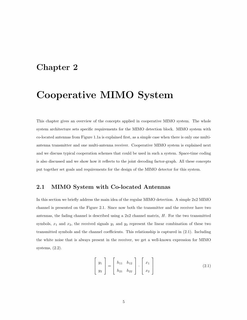
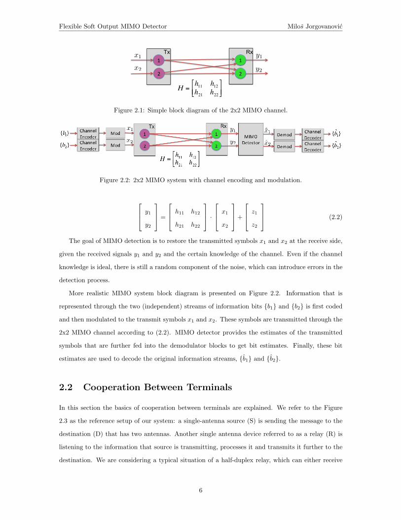
In this section we briefly address the main idea of the regular MIMO detection. A simple 2x2 MIMO
channel is presented on the Figure 2.1. Since now both the transmitter and the receiver have two
antennas, the fading channel is described using a 2x2 channel matrix, H. For the two transmitted
symbols, x1 and x2, the received signals y1 and y2 represent the linear combination of these two
transmitted symbols and the channel coefficients. This relationship is captured in (2.1). Including
the white noise that is always present in the receiver, we get a well-known expression for MIMO
systems, (2.2).
y1
y2
=
h11 h12
h21 h22
·
x1
x2
(2.1)
5
Flexible Soft Output MIMO Detector Milos Jorgovanovic
2 2
1 Rx
y2
y11
x1
x2
!
H =h11 h12h21 h22" # $
% & '
Tx
Figure 2.1: Simple block diagram of the 2x2 MIMO channel.
Figure 2.2: 2x2 MIMO system with channel encoding and modulation.
y1
y2
=
h11 h12
h21 h22
·
x1
x2
+
z1
z2
(2.2)
The goal of MIMO detection is to restore the transmitted symbols x1 and x2 at the receive side,
given the received signals y1 and y2 and the certain knowledge of the channel. Even if the channel
knowledge is ideal, there is still a random component of the noise, which can introduce errors in the
detection process.
More realistic MIMO system block diagram is presented on Figure 2.2. Information that is
represented through the two (independent) streams of information bits {b1} and {b2} is first coded
and then modulated to the transmit symbols x1 and x2. These symbols are transmitted through the
2x2 MIMO channel according to (2.2). MIMO detector provides the estimates of the transmitted
symbols that are further fed into the demodulator blocks to get bit estimates. Finally, these bit
estimates are used to decode the original information streams, {b1} and {b2}.
2.2 Cooperation Between Terminals
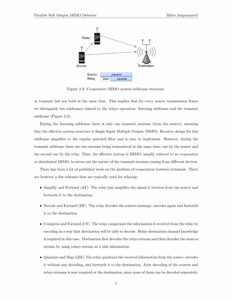
In this section the basics of cooperation between terminals are explained. We refer to the Figure
2.3 as the reference setup of our system: a single-antenna source (S) is sending the message to the
destination (D) that has two antennas. Another single antenna device referred to as a relay (R) is
listening to the information that source is transmitting, processes it and transmits it further to the
destination. We are considering a typical situation of a half-duplex relay, which can either receive
6
Flexible Soft Output MIMO Detector Milos Jorgovanovic
Figure 2.3: Cooperative MIMO system subframe structure.
or transmit but not both at the same time. This implies that for every source transmission frame
we distinguish two subframes related to the relays operation: listening subframe and the transmit
subframe (Figure 2.3).
During the listening subframe there is only one transmit antenna (from the source), meaning
that the effective system structure is Single Input Multiple Output (SIMO). Receiver design for this
subframe simplifies to the regular matched filter and is easy to implement. However, during the
transmit subframe there are two streams being transmitted at the same time, one by the source and
the second one by the relay. Thus, the effective system is MIMO, usually referred to as cooperative
or distributed MIMO, to stress out the nature of the transmit streams coming from different devices.
There has been a lot of published work on the problem of cooperation between terminals. There
are however a few schemes that are typically used for relaying:
• Amplify and Forward (AF) The relay just amplifies the signal it receives from the source and
forwards it to the destination.
• Decode and Forward (DF) The relay decodes the sources massage, encodes again and forwards
it to the destination.
• Compress and Forward (CF) The relay compresses the information it received from the relay by
encoding in a way that destination will be able to decode. Relay-destination channel knowledge
is required in this case. Destination first decodes the relays stream and then decodes the sources
stream by using relays stream as a side information.
• Quantize and Map (QM) The relay quantizes the received information from the source, encodes
it without any decoding, and forwards it to the destination. Joint decoding of the sources and
relays streams is now required at the destination, since none of them can be decoded separately.
7
Flexible Soft Output MIMO Detector Milos Jorgovanovic
Figure 2.4: Quantize and map scheme applied to the cooperative MIMO scenario.
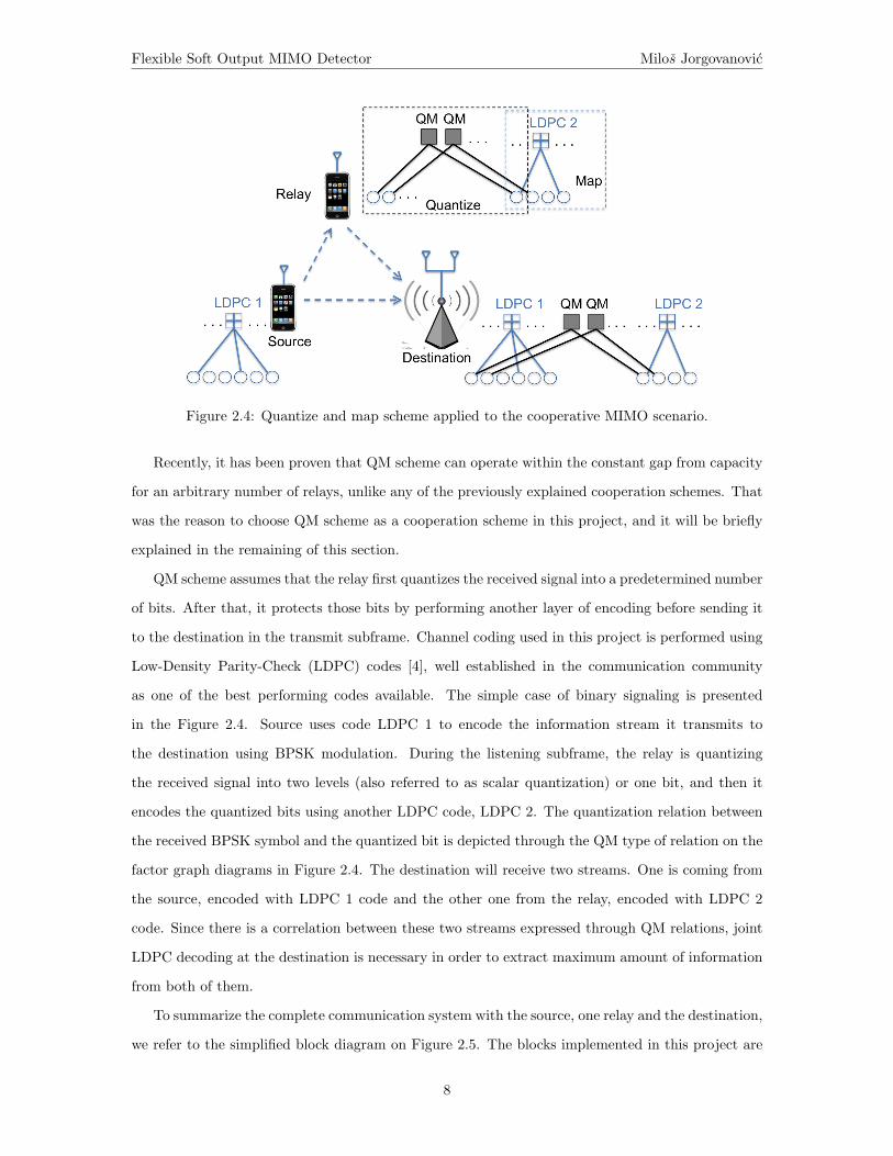
Recently, it has been proven that QM scheme can operate within the constant gap from capacity
for an arbitrary number of relays, unlike any of the previously explained cooperation schemes. That
was the reason to choose QM scheme as a cooperation scheme in this project, and it will be briefly
explained in the remaining of this section.
QM scheme assumes that the relay first quantizes the received signal into a predetermined number
of bits. After that, it protects those bits by performing another layer of encoding before sending it
to the destination in the transmit subframe. Channel coding used in this project is performed using
Low-Density Parity-Check (LDPC) codes [4], well established in the communication community
as one of the best performing codes available. The simple case of binary signaling is presented
in the Figure 2.4. Source uses code LDPC 1 to encode the information stream it transmits to
the destination using BPSK modulation. During the listening subframe, the relay is quantizing
the received signal into two levels (also referred to as scalar quantization) or one bit, and then it
encodes the quantized bits using another LDPC code, LDPC 2. The quantization relation between
the received BPSK symbol and the quantized bit is depicted through the QM type of relation on the
factor graph diagrams in Figure 2.4. The destination will receive two streams. One is coming from
the source, encoded with LDPC 1 code and the other one from the relay, encoded with LDPC 2
code. Since there is a correlation between these two streams expressed through QM relations, joint
LDPC decoding at the destination is necessary in order to extract maximum amount of information
from both of them.
To summarize the complete communication system with the source, one relay and the destination,
we refer to the simplified block diagram on Figure 2.5. The blocks implemented in this project are
8

Flexible Soft Output MIMO Detector Milos Jorgovanovic
Source
Relay
Destination
RF MOD ENC
RF Sync Quant ENC RF MOD
RF Sync MIMO Det
DEMOD
Chann Est
DEC
RF Sync
implemented
Figure 2.5: Simplified block diagram of the source-relay-destination system.
denoted at the receive side. Besides the MIMO detection and soft demodulation, the most challenging
parts for the implementation are the joint decoding block (described in more detail in one of the
next sections) and the synchronization part at the destination.
2.3 Space-Time Coding
Bit relationships presented in Figure 2.4 include the relationships that originate from LDPC coding
and quantization at the relay, but do not tell anything about the correlation through the channel.
Indeed, the bit relations introduced by the wireless channel will depend on the space-time coding
scheme that is used. Space-time coding depends on the purpose of use of the multiple antennas.
Transmit antennas can be used either to increase the diversity gain of the system or to increase the
multiplexing gain by sending many independent streams across different transmit antennas. This
latter scheme was indeed presented on the system diagram on Figure 2.2.
Coming back to the main goal of this project — to achieve multiplexing gain by using cooperation,
we concentrate to the schemes that are proven to provide multiplexing gain in the regular MIMO
system and discuss how they work in the cooperative MIMO case. Typical choice for achieving
multiplexing gain is Bell labs LAyered Space Time (BLAST) scheme that assumes codewords are
split into frames and transmitted across available antennas. There are two flavors of this scheme
typically used in the MIMO systems: Vertical BLAST (VBLAST) and Diagonal BLAST (DBLAST),
presented on Figure 2.6.
VBLAST is typically used in the MIMO systems where channel is fast-fading (changing fast
9

Flexible Soft Output MIMO Detector Milos Jorgovanovic
Figure 2.6: BLAST space-time coding schemes for MIMO.
enough) so that significant amount of interleaving can be achieved. It can be shown that under this
assumption, VBLAST achieves the capacity of the MIMO channel when joint decoding is used [3,5].
DBLAST is more complex for implementation, but it achieves the capacity of the MIMO channel
even under slow-fading channel conditions [3].
VBLAST scheme assumes that different parts of the same codeword are transmitted across
different antennas at the same time. In a cooperative setup, the relay listens to the sources codeword
(1S, 2S, 3S, etc.), processes the information using QM relaying scheme and transmits its share of
information (1R, 2R, 3R, etc.) during the same frame as the source, as shown on Figure 2.6. This
further implies that the sources and relays messages will be correlated not only through the QM
relations explained in the previous section, but also through the MIMO channel itself, since they are
sent at the same time, Figure 2.7a.
On the other hand, DBLAST assumes different parts of the same codeword are sent in different
frames (Figure 2.6), so there is no direct channel correlation between them. This is also shown
through factor graph representation in Figure 2.7. Now it can be seen that MIMO channel will
introduce the correlation between different codewords (1R and 2S, on Figure 2.7), however it will be
argued in Chapter 3 that MIMO detection technique we use can inherently break up these MIMO
relations to prevent them to further complicate the factor graph.
2.4 Joint LDPC Decoding
The nature of cooperation explained in the previous sections is that both the source and the relay
streams bear some information about the same original message. At this point, we can refer to
that original message as the source codeword (1S, 2S, 3S on Figure 2.6) and treat the relevant relay
10

Flexible Soft Output MIMO Detector Milos Jorgovanovic
Figure 2.7: Factor graphs capturing the relations between sources and relays messages for differentspace-time coding schemes: (a) VBLAST, (b) DBLAST.
codeword (1R, 2R, 3R Figure 2.6) as the side information that helps the destination to decode the
original message. If the source encodes the message in a way that destination can decode even
without side information of the relay, there is no point in using the relay. That is why source
can allow itself to encode the message with the higher rate than the one that destination would
normally be able to decode (without the relay). Using the additional (side) information that the
relays sends, destination is now able to decode the message successfully. Hence, effectively higher
data rate can be achieved in the system compared to the case without the relay and that’s how we
get the multiplexing gain. As was discussed previously, in order to use this side information in the
most effective way, QM relaying scheme that assumes joint decoding at the destination is used.
Joint LDPC decoding is done over the whole factor graph at the receive side, Figure 2.4. It
consists of the variable nodes (VAR), check nodes (CHK), quantize-and-map nodes (QM) and the
observation nodes (OBS). These nodes iteratively exchange messages among themselves until (ide-
ally) values of variable nodes converge to the bits that were sent at the source and the relay, Figure
2.8. The values that are passed between different nodes are the log likelihood ratios (LLRs) of the
variable bits, and they show how likely it is that certain bit has value 1 vs. value 0, as shown in
(2.3).
LLRi = lnP (bi = 1)P (bi = 0)
(2.3)
Each node in this factor graph performs different operation on the messages that it receives from
11

Flexible Soft Output MIMO Detector Milos Jorgovanovic
Figure 2.8: Factor graph for joint LDPC decoding at the destination.
the other nodes it is connected to. In the remaining of this section we briefly address how these
operations are done for each type of nodes:
• OBS nodes are the simplest, since they have only one connection. Due to the nature of the
message-passing algorithm for LDPC codes [4], these nodes have nothing to process and they
are always sending the same information (based on the observation of the particular bit) to
the VAR node they are connected to.
• VAR node is sending the message to every CHK and QM node it is connected to. That message
will represent the normalized sum of all the incoming messages into the particular VAR node,
except for the one which comes from the node the message is sent to [4].
• CHK node can be connected only to the VAR nodes. The message it sends to the particular
VAR node is represented as the marginalization [4] of all the incoming messages except for the
one that comes from that particular VAR node.
• Finally, operation of the QM node is explained in [12] and for the simple case of scalar quan-
tization that is explained in the previous section, it simplifies to the operation of the regular
two-edge CHK node.
Comparing factor graphs on Figure 2.7 and Figure 2.8, there is an apparent difference in the
connection of observation nodes. How we dealt with the MIMO relations from Figure 2.7 and
how we managed to break these up into single-edge connections on Figure 2.8 is described in the
next chapter when we discuss the connection between MMSE-SIC MIMO detection algorithm and
DBLAST space-time coding.
12
Chapter 3
Soft Output MIMO Detector for
DBLAST
MIMO Detector design is one of the most complex parts of the MIMO receiver baseband. The
complexity depends typically on the number of transmit and receive antennas, but also on the
constellation size for detectors that use tree search. There are a few approaches to the detection
problem, which further evolve into number of different architectures.
Two basic detection methods introduced in chapter 1 are linear detectors and Maximum Like-
lihood (ML) detectors that use some form of tree search. Both of these two types are widely used
in the current and future wireless communication systems that deploy MIMO. There are quite a
few algorithms and designs for both groups proposed in the literature [3], [9], [19], [7], [18] . Basic
difference is that linear detectors are much simpler and require less resources. ML detectors are more
complex since they are in general not trying to estimate the transmitted symbol, but to identify one
which was most likely to have been sent. Generating soft bit outputs for ML type of detectors is
particularly difficult problem and also requires very complex computation. Having in mind one of
the goals of this project, to design a low complexity MIMO detector that will have soft bit outputs,
the architecture of choice was the linear MMSE-SIC detector.
The architecture and performance of the MIMO detector also depends on the space-time scheme
being used, as discussed in chapter 2. In particular, in this chapter we are concentrating on MIMO
detectors for DBLAST scheme, Figure 3.1. Note that MIMO detection is the same whether streams
are coming from the same multiple-antenna device, or from different single-antenna devices, because
of the DBLAST. Difference will come in terms of channel decoding,. Regular MIMO would use
13

Flexible Soft Output MIMO Detector Milos Jorgovanovic
CW A2 CW A1 CW B1
CW B2 CW C1
CW C2 CW D1
CW D2 CW E1
CW A3 CW B3 CW C3 CW A4 CW B4 Stream 4
Stream 3 Stream 2 Stream 1
Figure 3.1: DBLAST space-time coding.
regular LDPC code, whereas cooperative MIMO would use joint decoding strategy described in
chapter 2. Number of streams is typically equal to the number of transmit antennas (4 in our
example on Fig. 3.1) and that is the case we will be considering in this analysis.
Special attention will be given to explaining the difference between the hard and the soft detec-
tion. The implementation greatly depends on whether the channel decoder deals with hard bits or
soft bit inputs (LLRs). In our case, LDPC codes are known to provide much better performance
when fed with soft bit estimates, so the MIMO detector is preferred to have soft bit outputs.
3.1 Linear Detectors
Linear detectors assume that the estimates of the transmitted symbols are obtained through linear
processing of the received signal. To clarify the concept, let’s rewrite the expression (2.2) in the
more general form:
y1...
ynr
=
h1,1 ... h1,nr
.... . .
...
hnt,1 ... hnt,nr
·
x1
...
xnt
+
z1...
znr
, (3.1)
or in the form of vectors:
y = H ·x+ z, (3.2)
where x is the transmitted symbol vector, H is the channel matrix and z is the gaussian noise.
Number of transmit and receive antennas are denoted by nt and nr, respectively. Without the loss
of generality, we can assume that the covariance matrices of the transmitted symbol vector and the
noise are given with (3.3) and (3.4):
Kx = I (3.3)
14

Flexible Soft Output MIMO Detector Milos Jorgovanovic
Kz =1
SNR· I (3.4)
In order to get the soft symbol estimates of the transmitted vector, we perform the linear pro-
cessing of the received vector. This assumes the following operation:
x = F · y, (3.5)
where F is the filter matrix that depends on the linear detection method being used. We must
keep in mind that the decoder operates with bits, so demodulation would have to be done based on
the soft symbol estimates that linear filter provides. As indicated in the previous chapter, LDPC
decoder prefers soft bit inputs. That means that these would have to be generated based on the soft
symbol estimates from the MIMO detector. This demodulation is explained in the detail later in this
chapter and at this point we will just point out that it is a very simple extension of the regular (hard
output) MMSE-SIC detector. In the following section two most common linear detection strategies
will be explained.
3.1.1 MMSE Detector
Minimum mean square error (MMSE) detection is well known concept in estimation theory. As the
name suggests, it tends to minimize the mean square error of the detection. In case of MIMO, we
are indeed looking for the linear detector, as described by (3.2), so it is also referred to as the linear
least square error (LLSE) detector. The MIMO community typically use MMSE as a default name
and the same name will be used throughout this work.
It can be shown that the linear MMSE estimator has a very simple form given the second order
statistics of the transmitted vector x and the observation y and this expression is given with (3.6).
If x and y are jointly Gaussian, the LLSE solution becomes equivalent to the general MMSE.
FMMSE = KxyK−1y , (3.6)
Since the relation between the signal being estimated and the observation is given with (3.2)
and the covariance matrices of transmitted signal and the noise are known, we get the following
expression for the linear MMSE filter:
FMMSE = HH(1
SNR· I +HHH)−1 (3.7)
15
Flexible Soft Output MIMO Detector Milos Jorgovanovic
MMSE Stream 4
Z-‐1
Decode
MMSE Stream 3
MMSE Stream 2
MMSE Stream 1
Z-‐1
Z-‐1
{y} {b}
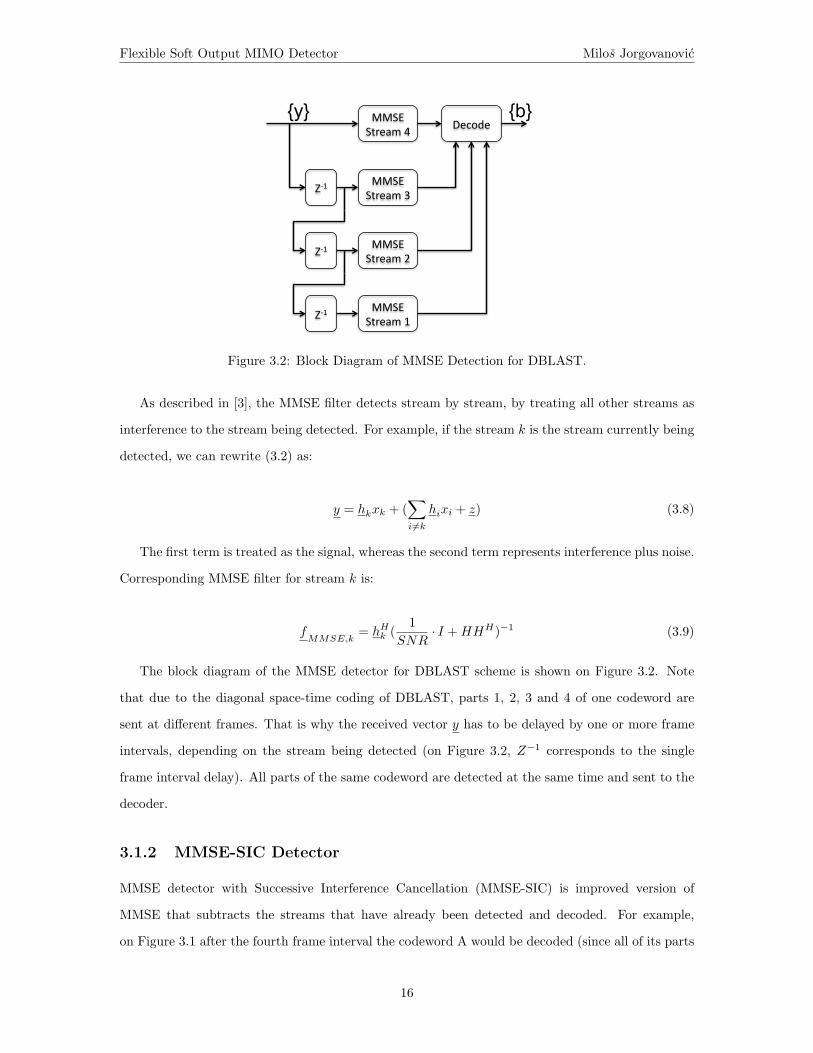
Figure 3.2: Block Diagram of MMSE Detection for DBLAST.
As described in [3], the MMSE filter detects stream by stream, by treating all other streams as
interference to the stream being detected. For example, if the stream k is the stream currently being
detected, we can rewrite (3.2) as:
y = hkxk + (∑
i6=khixi + z) (3.8)
The first term is treated as the signal, whereas the second term represents interference plus noise.
Corresponding MMSE filter for stream k is:
fMMSE,k
= hHk (1
SNR· I +HHH)−1 (3.9)
The block diagram of the MMSE detector for DBLAST scheme is shown on Figure 3.2. Note
that due to the diagonal space-time coding of DBLAST, parts 1, 2, 3 and 4 of one codeword are
sent at different frames. That is why the received vector y has to be delayed by one or more frame
intervals, depending on the stream being detected (on Figure 3.2, Z−1 corresponds to the single
frame interval delay). All parts of the same codeword are detected at the same time and sent to the
decoder.
3.1.2 MMSE-SIC Detector
MMSE detector with Successive Interference Cancellation (MMSE-SIC) is improved version of
MMSE that subtracts the streams that have already been detected and decoded. For example,
on Figure 3.1 after the fourth frame interval the codeword A would be decoded (since all of its parts
16
Flexible Soft Output MIMO Detector Milos Jorgovanovic
would have been detected). After codeword A is (successfully) decoded, we cancel part A2 from the
received vectors in the second frame, part A3 from the received vectors in the third frame and part
A4 from the received vectors in the fourth frame. This means that in the next processing step, parts
B1, B2, B3 will see no interference from codeword A and their detection should be improved. After
all parts of codeword B are detected and the codeword B is decoded, its interference is cancelled
and so on.
Going back to the general case of n streams, it can be concluded that when stream k is being
detected, streams k+ 1, ..., n have been detected, decoded and cancelled from the received vector y.
That means that the channel matrix H became ”thinner” by taking out the columns k + 1, ..., n.
Also the transmitted vector is shortened by taking out symbols that have already been detected and
decoded. If we denote this reduced channel matrix with H(k) and the reduced transmit vector with
xk, we can rewrite equation (3.2) as:
yk
= H(k) ·xk + z (3.10)
or
yk
= hkxk + (k−1∑
i=1
hixi + z), (3.11)
where yk
is the received vector after last n− k streams have been cancelled, as presented by the
next expression:
yk
= y −n∑
i=k+1
hixi (3.12)
Now it is clear that due to cancellation the amount of interference will get smaller for streams
with lower index, as shown in (3.11) and so detection of those streams will be improved compared to
the MMSE detector. Performance comparison between MMSE and MMSE-SIC detection schemes
is further explained in [3].
Similarly, the MMSE-SIC filter equation can be derived for each stream separately. Similarly to
how expression (3.9) was derived from (3.2), based on expression (3.10) we can derive the MMSE
for stream k under SIC condition:
fSIC,k
= hHk (1
SNR· I +H(k)H
H(k))−1 (3.13)
17
Flexible Soft Output MIMO Detector Milos Jorgovanovic
MMSE Stream 4
Z-‐1
Decode
Cancel Stream 4
MMSE Stream 3
Cancel Streams 3
MMSE Stream 2
Cancel Streams 2
MMSE Stream 1
Z-‐1
Z-‐1
Z-‐1 Z-‐1 Z-‐1 {y} {b}
Figure 3.3: Block Diagram of MMSE-SIC Detection for DBLAST.
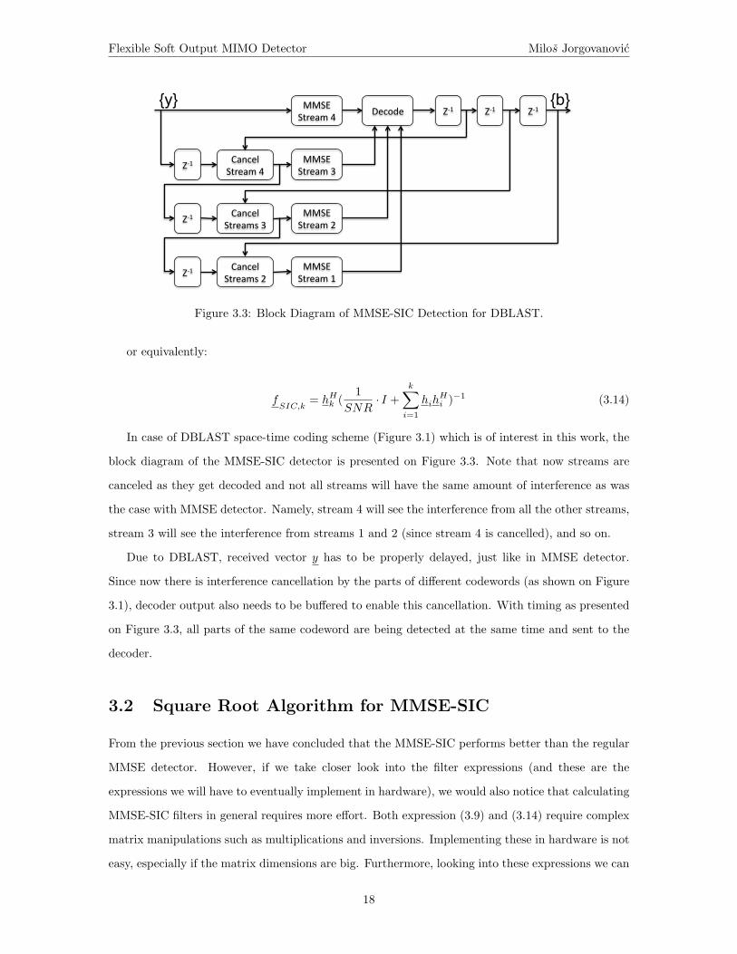
or equivalently:
fSIC,k
= hHk (1
SNR· I +
k∑
i=1
hihHi )−1 (3.14)
In case of DBLAST space-time coding scheme (Figure 3.1) which is of interest in this work, the
block diagram of the MMSE-SIC detector is presented on Figure 3.3. Note that now streams are
canceled as they get decoded and not all streams will have the same amount of interference as was
the case with MMSE detector. Namely, stream 4 will see the interference from all the other streams,
stream 3 will see the interference from streams 1 and 2 (since stream 4 is cancelled), and so on.
Due to DBLAST, received vector y has to be properly delayed, just like in MMSE detector.
Since now there is interference cancellation by the parts of different codewords (as shown on Figure
3.1), decoder output also needs to be buffered to enable this cancellation. With timing as presented
on Figure 3.3, all parts of the same codeword are being detected at the same time and sent to the
decoder.
3.2 Square Root Algorithm for MMSE-SIC
From the previous section we have concluded that the MMSE-SIC performs better than the regular
MMSE detector. However, if we take closer look into the filter expressions (and these are the
expressions we will have to eventually implement in hardware), we would also notice that calculating
MMSE-SIC filters in general requires more effort. Both expression (3.9) and (3.14) require complex
matrix manipulations such as multiplications and inversions. Implementing these in hardware is not
easy, especially if the matrix dimensions are big. Furthermore, looking into these expressions we can
18
Flexible Soft Output MIMO Detector Milos Jorgovanovic
conclude that the MMSE filters for different streams reuse the same term, so matrix inversion would
have to be done only once for each channel instance. On the other hand, from expression (3.14) it
appears that for each MMSE-SIC filter we have to invert different matrix and that MMSE-SIC will
require significant increase in computation compared to standard MMSE.
In this section we present a well known algorithm for calculating MMSE-SIC filter coefficients,
given the channel matrix and the SNR value of the link. It was first published by Hassibi [9] in 2000
and later extended in [19], [17], [10]. Main strength of this algorithm is that it does not include any
matrix multiplication or inversion, so main computation bottleneck is avoided. Furthermore, it uses
partial results of the MMSE-SIC filters for higher streams in the computation of the filters for lower
streams which also reduces the computation complexity.
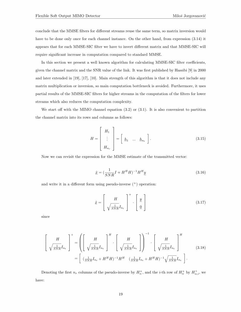
We start off with the MIMO channel equation (3.2) or (3.1). It is also convenient to partition
the channel matrix into its rows and columns as follows:
H =
H1
...
Hnr
=[h1 ... hnt
]. (3.15)
Now we can revisit the expression for the MMSE estimate of the transmitted vector:
x = (1
SNRI +HHH)−1HHy (3.16)
and write it in a different form using pseudo-inverse (+) operation:
x =
H√
1SNRInt
+
·
y
0
(3.17)
since
H√
1SNRInt
+
=
H√
1SNRInt
H
·
H√
1SNRInt
−1
·
H√
1SNRInt
H
=[
( 1SNRInt +HHH)−1HH ( 1
SNRInt +HHH)−1√
1SNRInt
].
(3.18)
Denoting the first nr columns of the pseudo-inverse by H+α , and the i-th row of H+
α by H+α,i, we
have:
19

Flexible Soft Output MIMO Detector Milos Jorgovanovic
x = H+α y (3.19)
and
xi = H+α,iy. (3.20)
H+α,i is referred to as the MMSE filter for the i-th stream and is equivalent to the expression
obtained in the previous section, (3.9). We can also find the covariance matrix of the estimation
error (x− x) to be:
P = E[(x− x)(x− x)H ] = (1
SNRInt +HHH)−1 (3.21)
or using the pseudo-inverse:
P =
H√
1SNRInt
+
H√
1SNRInt
+
H
. (3.22)
In the original square-root algorithm proposed by Hassibi in [9], there is additional complexity
of finding the strongest stream and start the detection with that one first. That is the standard
procedure for VBLAST space-time coding and SIC type of detector. In case of DBLAST, there is
predetermined order of detection (starting from the highest stream, nt) and this additional step of
ordering the streams is not required. So, we detect the stream nt using (3.9) or equivalently H+α,nt .
After detecting stream nt and decoding the codeword it belongs to, we subtract its influence to the
other streams as described in (3.12), deflate channel matrix H to H(nt−1) by taking out last column
and reduce the dimension of the estimation problem from nt to nt − 1. The channel equation now
becomes:
ynt−1
= H(nt−1)xnt−1 + z. (3.23)
In the next iteration, we would have to find H+(nt−1),α and P(nt−1) for this new expression and
so on. The goal is to somehow reuse the parameters we have already calculated, without doing
additional matrix inversions. In order to see the connection between the H+α and H+
(nt−1),α, let us
rewrite the augmented channel matrix through the QR decomposition:
20
Flexible Soft Output MIMO Detector Milos Jorgovanovic
H√
1SNRInt
= QR =
Qα
Q2
R, (3.24)
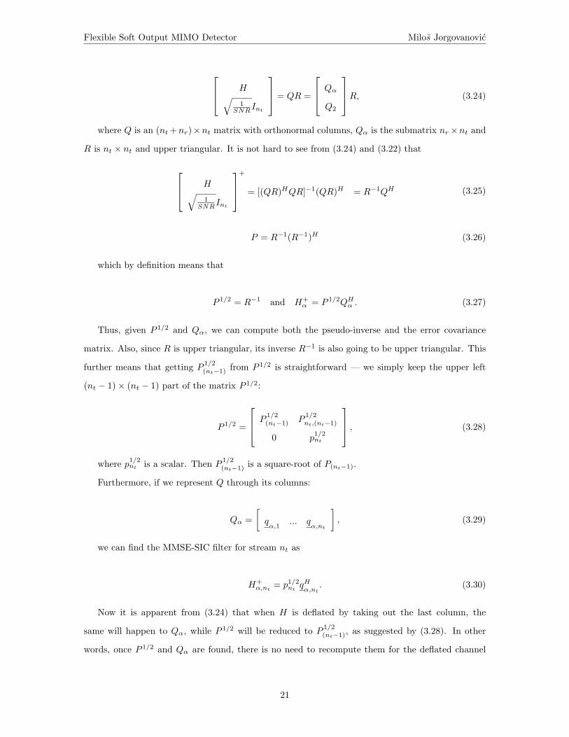
where Q is an (nt +nr)×nt matrix with orthonormal columns, Qα is the submatrix nr×nt and
R is nt × nt and upper triangular. It is not hard to see from (3.24) and (3.22) that
H√
1SNRInt
+
= [(QR)HQR]−1(QR)H = R−1QH (3.25)
P = R−1(R−1)H (3.26)
which by definition means that
P 1/2 = R−1 and H+α = P 1/2QHα . (3.27)
Thus, given P 1/2 and Qα, we can compute both the pseudo-inverse and the error covariance
matrix. Also, since R is upper triangular, its inverse R−1 is also going to be upper triangular. This
further means that getting P1/2(nt−1) from P 1/2 is straightforward — we simply keep the upper left
(nt − 1)× (nt − 1) part of the matrix P 1/2:
P 1/2 =
P
1/2(nt−1) P
1/2nt,(nt−1)
0 p1/2nt
, (3.28)
where p1/2nt is a scalar. Then P
1/2(nt−1) is a square-root of P(nt−1).
Furthermore, if we represent Q through its columns:
Qα =[qα,1
... qα,nt
], (3.29)
we can find the MMSE-SIC filter for stream nt as
H+α,nt = p1/2
nt qHα,nt
. (3.30)
Now it is apparent from (3.24) that when H is deflated by taking out the last column, the
same will happen to Qα, while P 1/2 will be reduced to P1/2(nt−1), as suggested by (3.28). In other
words, once P 1/2 and Qα are found, there is no need to recompute them for the deflated channel
21
Flexible Soft Output MIMO Detector Milos Jorgovanovic
matrix H(nt−1). The only thing we have to do is to find the MMSE-SIC filter vectors by simple
multiplication of a vector and a constant, as suggested by (3.30).
Next thing is to find these two matrices initially, without doing matrix multiplications or inver-
sions. To do that, the traditional square-root algorithm explained in [15] has been modified in [9]
to accommodate the problem at hand.
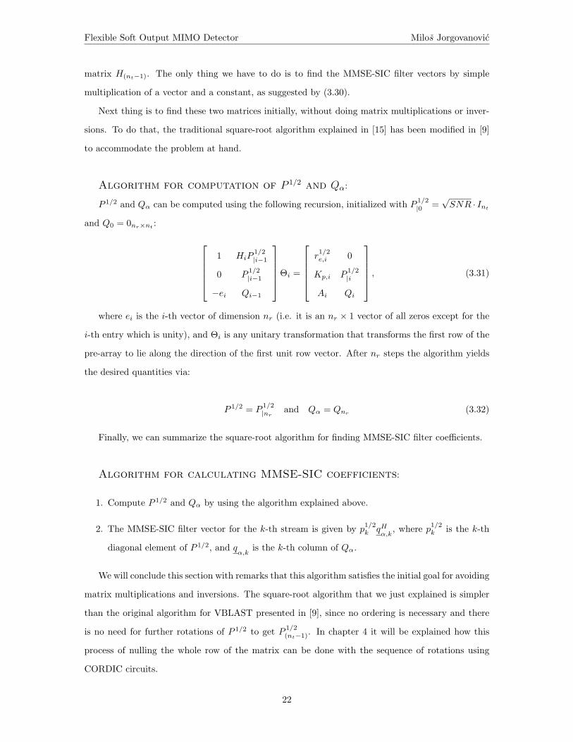
Algorithm for computation of P 1/2 and Qα:
P 1/2 and Qα can be computed using the following recursion, initialized with P 1/2|0 =
√SNR · Int
and Q0 = 0nr×nt :
1 HiP1/2|i−1
0 P1/2|i−1
−ei Qi−1
Θi =
r1/2e,i 0
Kp,i P1/2|i
Ai Qi
, (3.31)
where ei is the i-th vector of dimension nr (i.e. it is an nr × 1 vector of all zeros except for the
i-th entry which is unity), and Θi is any unitary transformation that transforms the first row of the
pre-array to lie along the direction of the first unit row vector. After nr steps the algorithm yields
the desired quantities via:
P 1/2 = P1/2|nr and Qα = Qnr (3.32)
Finally, we can summarize the square-root algorithm for finding MMSE-SIC filter coefficients.
Algorithm for calculating MMSE-SIC coefficients:
1. Compute P 1/2 and Qα by using the algorithm explained above.
2. The MMSE-SIC filter vector for the k-th stream is given by p1/2k qH
α,k, where p1/2
k is the k-th
diagonal element of P 1/2, and qα,k
is the k-th column of Qα.
We will conclude this section with remarks that this algorithm satisfies the initial goal for avoiding
matrix multiplications and inversions. The square-root algorithm that we just explained is simpler
than the original algorithm for VBLAST presented in [9], since no ordering is necessary and there
is no need for further rotations of P 1/2 to get P 1/2(nt−1). In chapter 4 it will be explained how this
process of nulling the whole row of the matrix can be done with the sequence of rotations using
CORDIC circuits.
22

Flexible Soft Output MIMO Detector Milos Jorgovanovic
3.3 Algorithm Extension for Soft Bit Output Generation
In this section we show how to generate necessary parameters for soft bit demodulation from the
square-root algorithm that was described in the previous section. We argue this is done with the
minimum amount of added computation compared to the hard output case. In order to show the
relationship between these parameters and the MMSE-SIC filter coefficients, the whole process of
MMSE-SIC detection for an arbitrary stream k will be shown in detail.
Starting with the equation (3.11), we can short it down by denoting all the interference that
stream k sees as zk:
yk
= hkxk + zk, (3.33)
where
zk =k−1∑
i=1
hixi + z. (3.34)
This noise+interference term, zk, is now not white any more. Still, we can find its second order
statistics as:
Kzk= E[zkz
Hk ] =
k−1∑
i=1
hihHi +
1SNR
I. (3.35)
In order to detect symbol xk from equation (3.33), first we have to whiten the noise zk. This is
done by multiplying the whole expression such that the resulting noise has covariance matrix equal
to identity:
K−1/2zk
yk
= K−1/2zk
hkxk +K−1/2zk
zk. (3.36)
Once the noise is white, the optimal detection assumes matched filtering. After we apply matched
filter to (3.36), we get the following:
hHk K−1/2zk
K−1/2zk
yk
= hHk K−1/2zk
K−1/2zk
hkxk + hHk K−1/2zk
K−1/2zk
zk (3.37)
hHk K−1zkyk
= hHk K−1zkhkxk + hHk K
−1zkzk (3.38)
23
Flexible Soft Output MIMO Detector Milos Jorgovanovic
hHk K−1zkyk
hHk K−1zk hk
= xk +hHk K
−1zkzk
hHk K−1zk hk
. (3.39)
This means that practically the detection of stream k reduces to the scalar detection. Further-
more, since after whitening the noise components were independent Gaussians, the noise will remain
Gaussian after the match filter was applied. We can rewrite (3.39) in the more clear form:
yk = xk + zk, (3.40)
where from (3.39):
σ2xk
= 1 (3.41)
zk ∼ (0,1
hHk K−1zk hk
) (3.42)
SINRk =σ2xk
σ2zk
= hHk K−1zkhk (3.43)
It is shown in the next section that the parameters needed for the soft bit output generation are
yk and SINRk. The output from the square root algorithm however, is only the MMSE estimate of
the current stream, xk, and the MMSE-SIC filter coefficients fSIC,k given by (3.14) or alternatively
by (3.30). In the remaining of this section the novel way of computing yk and SINRk will be
presented.
Using (3.40) it is easy to find MMSE estimate for xk:
xk =σ2xk
σ2xk
+ σ2zk
yk
=SINRk
1 + SINRkyk,
(3.44)
or equivalently:
yk = (1 +1
SINRk)xk. (3.45)
So, once we calculate the SINR for stream k there is a straightforward relation between the
MMSE estimate of the transmitted symbol xk and the parameter yk. Now the relationship between
the MMSE filter coefficients and the SINRk will be shown.
24

Flexible Soft Output MIMO Detector Milos Jorgovanovic
By combining expressions (3.35) and (3.43), we get:
SINRk = hHk (1
SNR· I +
k−1∑
i=1
hihHi )−1hk, (3.46)
which fairly resembles the expression for MMSE filter coefficients, (3.14). The summations in
the brackets does not however match perfectly between the two expressions and on order to find the
exact relationship, the matrix inversion lemma can be used:
fSIC,k
= hHk (1
SNR· I +
k∑
i=1
hihHi )−1
= hHk (Bk + hkhHk )−1
= hHk B−1k −
hHk B−1k hkh
Hk B−1k
1 + hHk B−1k hk
= hHk B−1k
11 + hHk B
−1k hk
,
(3.47)
where
Bk = (1
SNR· I +
k−1∑
i=1
hihHi ). (3.48)
Now it is easy to see that SINRk can be represented as:
SINRk = hHk B−1k hk (3.49)
and similarly using (3.47):
fSIC,k
hk =hHk B
−1k hk
1 + hHk B−1k hk
=SINRk
1 + SINRk.
(3.50)
In the next step we get the exact expression for the SINR of stream k:
SINRk =fSIC,k
hk
1− fSIC,k
hk. (3.51)
Now it can be concluded that by filtering the channel itself (i.e. the column of the channel matrix
H that corresponds to the stream being detected) and performing the operation
f(x) =x
1− x (3.52)
25

Flexible Soft Output MIMO Detector Milos Jorgovanovic
we can get the SINR of every stream. Note that this operation represents a very simple extension
to the algorithm that was described in the previous section. In terms of hardware we need to add
another filter block and implement a simple look-up table for operation given in (3.52). In order
to get the received symbol yk in (3.40), expression (3.45) can be further simplified by substituting
SINRk from (3.51) to get:
yk =1
fSIC,k
hkxk, (3.53)
or written in another form:
yk = (1 +1− f
SIC,khk
1− (1− fSIC,k
hk))xk, (3.54)
which suggests that the same look-up table from (3.52) can be used to calculate SINRk as well
as yk.
3.4 Soft Bit Output Generation
Next, we show how the soft bit estimates are obtained using the scalar expression given with (3.40)
and the information about the second order statistics of the signal and the noise (3.41), (3.42) and
(3.43). The soft bit estimates are typically represented through the Log Likelihood Ratios (LLR),
defined as:
LLRi = lnP (bi = 1|yk)P (bi = 0|yk)
, (3.55)
where bit bi is any bit in the constellation of the transmitted symbol xk. If we assume that every
bit can be ’1’ or ’0’ with the same probability and that every symbol in the constellation is equally
likely at the transmit side, we can further write:
LLRi = ln
fyk|bi (yk|bi=1) ·P (bi=1)
fyk (yk)
fyk|bi (yk|bi=0) ·P (bi=0)
fyk (yk)
= lnfyk|bi(yk|bi = 1)fyk|bi(yk|bi = 0)
= ln
∑
xk,bi=1
fyk|xk(yk|xk) ·P (xk)
∑
xk,bi=0
fyk|xk(yk|xk) ·P (xk)
(3.56)
26

Flexible Soft Output MIMO Detector Milos Jorgovanovic
LLRi = ln
∑
xk,bi=1
e− 1
2σ2zk
|yk−xk|2
∑
xk,bi=0
e− 1
2σ2zk
|yk−xk|2(3.57)
The equation (3.57) looks rather complex and for the high order constellations such as 64QAM
implementing the exact expression in hardware would take a forbidden amount of resources. There
are however standard ways to simplify (3.57), one of them being the ”max-log” approximation. It
assumes that the sum of exponentials can be approximated by the most dominant term, namely one
with the highest exponent (3.58). Now this expression can be further simplified to get rid of the
exponentials and the logarithm (3.59) and then finally written in the short form (3.60).
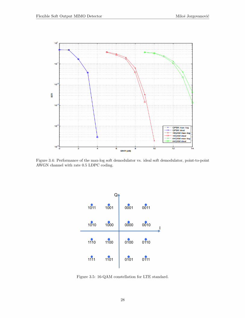
Figure 3.4 shows the performance difference when ideal soft bit demodulator is used (3.57), versus
the performance when soft bits are generated using the max-log approximation. This approximation
is indeed exact for the QPSK constellation. The difference in performance is very small for 16-QAM
(around 0.2dB) and slightly higher for 64-QAM (around 0.4dB), for point-to-point AWGN channel
and the rate 1/2 LDPC decoding (blocklength is 2040).
LLRi = lnmaxxk,bi=1
{e− 1
2σ2zk
|yk−xk|2}
maxxk,bi=0
{e− 1
2σ2zk
|yk−xk|2}(3.58)
LLRi = maxxk,bi=1
{− 12σ2
zk
|yk − xk|2} − maxxk,bi=0
{− 12σ2
zk
|yk − xk|2} (3.59)
LLRi =1
2σ2zk
( minxk,bi=1
{|yk − xk|2} − minxk,bi=0
{|yk − xk|2}) (3.60)
Even without doing any approximations, if we take a look at how the standard constellation for
Long Term Evolution (LTE) standard is defined - using Gray mapping, we can notice regularities
that can help us simplify (3.58) even further. For example, for 16QAM constellation presented on
Figure 3.5 which is given by the LTE standard, we can clearly see that one half of the symbols (left
half plane with 8 symbols) has bit 1 equal to ’1’ and the other one has bit 1 equal to ’0’. Similarly,
we can draw specific regions on the constellation diagram for each bit (Figure 3.6a). This effectively
means that if the received symbol yk falls into the left half plane (denoted by b1 = 1), the hard
demodulator would return b1 of the transmitted symbol xk to have value ’1’. Still, as we concluded
from chapter 2, hard demodulation is not good enough and we have to feed the LDPC decoder with
27
Flexible Soft Output MIMO Detector Milos Jorgovanovic
Figure 3.4: Performance of the max-log soft demodulator vs. ideal soft demodulator, point-to-pointAWGN channel with rate 0.5 LDPC coding.
1011 1001
1010 1000
0001 0011
0000 0010
1110 1100
1111 1101
0100 0110
0101 0111
I
Q
Figure 3.5: 16-QAM constellation for LTE standard.
28

Flexible Soft Output MIMO Detector Milos Jorgovanovic
(a) (b)
b1 = 1 b1 = 0
b3 = 1 b3 = 0 b3 = 3
b2 = 0
b2 = 1
b4 = 1
b4 = 1
b4 = 0
1011 1001
1010 1000
0001 0011
0000 0010
1110 1100
1111 1101
0100 0110
0101 0111
I
Q
1011 1001
1010 1000
0001 0011
0000 0010
1110 1100
1111 1101
0100 0110
0101 0111
I
Q
Figure 3.6: 16-QAM constellation divided into detection regions for each bit.
the soft bit values - LLRs.
From Figure 3.6b it can be concluded that each bit in 16-QAM constellation takes the same
value either in columns or in rows of the 4x4 square of symbols (thus we could draw the regions
for each bit which are straight dashed lines on Figure 3.6). Intuitively, it means that when we are
trying to determine if the demodulated bit is ’1’ or ’0’, one of the dimensions is going to be way
more important than the other one. Same conclusion can be made for other constellations given by
the LTE standard.
If we concentrate specifically on the max-log approximation from (3.60), we can indeed prove
that each demodulated bit depends exclusively on one dimension of the 16-QAM constellation -
bits 1 and 3 depend on the real part (I) and bits 2 and 4 on the complex part (Q). This implies
that instead of calculating |yk − xk|2 which deals with complex numbers, we can deal only with
real or imaginary parts of these values, depending on the bit whose LLR we are currently trying to
calculate.
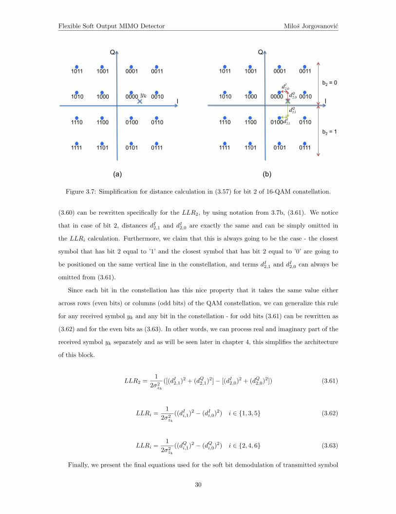
In order to prove this simplification, we refer to Figure 3.7a and show how LLR2 is calculated
for a given received symbol yk (marked with an ’x’). If expression (3.57) is used, we would have to
calculate distances from the received symbol yk to every single constellation point and then form
corresponding sum of exponentials. On the other hand, if expression (3.60) is used only two distances
would have to be calculated - one to the nearest symbol in the constellation that has bit 2 equal to
’1’ and the second one to the nearest symbol in the constellation that has bit 2 equal to ’0’.
These distances are broken into the I and Q components, as shown on Figure 3.7b. Expression
29
Flexible Soft Output MIMO Detector Milos Jorgovanovic
(a) (b)
1011 1001
1010 1000
0001 0011
0000 0010
1110 1100
1111 1101
0100 0110
0101 0111
I
Q
b2 = 0
b2 = 1
!
d2,0I
!
d2,0Q
!
d2,1I
!
d2,1Q
1011 1001
1010 1000
0001 0011
0000 0010
1110 1100
1111 1101
0100 0110
0101 0111
I
Q
yk
Figure 3.7: Simplification for distance calculation in (3.57) for bit 2 of 16-QAM conatellation.
(3.60) can be rewritten specifically for the LLR2, by using notation from 3.7b, (3.61). We notice
that in case of bit 2, distances dI2,1 and dI2,0 are exactly the same and can be simply omitted in
the LLRi calculation. Furthermore, we claim that this is always going to be the case - the closest
symbol that has bit 2 equal to ’1’ and the closest symbol that has bit 2 equal to ’0’ are going to
be positioned on the same vertical line in the constellation, and terms dI2,1 and dI2,0 can always be
omitted from (3.61).
Since each bit in the constellation has this nice property that it takes the same value either
across rows (even bits) or columns (odd bits) of the QAM constellation, we can generalize this rule
for any received symbol yk and any bit in the constellation - for odd bits (3.61) can be rewritten as
(3.62) and for the even bits as (3.63). In other words, we can process real and imaginary part of the
received symbol yk separately and as will be seen later in chapter 4, this simplifies the architecture
of this block.
LLR2 =1
2σ2zk
([(dI2,1)2 + (dQ2,1)2]− [(dI2,0)2 + (dQ2,0)2]) (3.61)
LLRi =1
2σ2zk
((dIi,1)2 − (dIi,0)2) i ∈ {1, 3, 5} (3.62)
LLRi =1
2σ2zk
((dQi,1)2 − (dQi,0)2) i ∈ {2, 4, 6} (3.63)
Finally, we present the final equations used for the soft bit demodulation of transmitted symbol
30

Flexible Soft Output MIMO Detector Milos Jorgovanovic
xk, given the parameters yk and SINRk as defined in (3.40), (3.42) and (3.43). x1k,i and x0
k,i denote
the closest symbols to the received symbol yk that have bit i equal to ’1’ and ’0’, respectively.
LLRk,i =12SINRk · (real{yk − x1
k,i}2 − real{yk − x0k,i}2) i ∈ {1, 3, 5} (3.64)
LLRk,i =12SINRk · (imag{yk − x1
k,i}2 − imag{yk − x0k,i}2) i ∈ {2, 4, 6} (3.65)
3.5 2x2 MIMO Performance of the Proposed Algorithm
In this section we present the performance comparison between the idealized MMSE-SIC soft bit
output MIMO detector and the proposed solution. Simulations are done in MATLAB using r = 1/2
LDPC code of blocklength 2040. System is 2x2 MIMO with DBLAST space-time coding and per-
symbol interleaving, meaning that bits of the same codeword are modulated to QAM symbols and
each symbol is interleaved to see different MIMO channel. The channel is flat fading, with channel
gains of Rayleigh distribution.
Figure 3.8 shows BER curves for three combinations of MIMO detection and soft bit demodula-
tion algorithms, explained below. Performance curves are given for QPSK, 16-QAM and 64-QAM
modulations.
• ”ideal-ideal” refers to the ideal MMSE-SIC algorithm (with floating point matrix computations
using (3.14)) and ideal soft bit demodulation (3.57) for all 3 QAM modulations. This is blue
set of curves on Figure 3.8.
• ”ideal-maxLog” refers to the ideal MMSE-SIC algorithm as in the previous case and max-log
approximation used for the soft bit demodulation. This is green set of curves on Figure 3.8.
• ”sqrtAlg-maxLog” refers to the square-root algorithm that is used for calculating the MMSE-
SIC coefficients as explained earlier in this section and the max-log approximation used for
the soft bit demodulation. This is red set of curves on Figure 3.8 and they correspond to the
actual implemented soft output MIMO detector.
Apparently, the difference in performance is quite small and is kept to within a fraction of a dB
even for 64-QAM constellation. Furthermore, we can tell what is the difference in performance due
to two approximations introduced in this work - square-root algorithm and soft bit demodulation.
Namely, the performance difference between the blue and the green curves reflects the difference
31
Flexible Soft Output MIMO Detector Milos Jorgovanovic
between the ideal soft demodulation algorithm (3.57) and the suggested solution for soft demodula-
tion. This solution includes approximative way of calculating parameters yk and SINRk using LUT
and approximate (3.57) using max-log approximation, (3.60). For QPSK these two curves actually
overlap, since max-log approximation is indeed exact.
The performance difference between the green and the red curves is the difference between using
the ideal way to calculate MMSE-SIC coefficients and using the square-root algorithm. We see
that this difference is very small for all three modulations, which implies that square-root algorithm
proves to be a very good approximation for MMSE-SIC coefficients calculation.
Also, these results approximately match the difference in performance for point-to-point AWGN
channel given on Figure 3.4, which shows that the approximations we have made so far are good for
both point-to-point and the MIMO case.
32

Flexible Soft Output MIMO Detector Milos Jorgovanovic
Figure 3.8: BER curves for 2x2 MIMO with DBLAST and per symbol interleaving — ideal MMSE-SIC and proposed design using square-root algorithm and max-log soft demodulator.
33
Chapter 4
Hardware Implementation
This chapter describes design architecture and hardware implementation of the MMSE-SIC MIMO
detector. These are based on the algorithms and calculations presented in chapter 3, and are adjusted
to meet some general design goals imposed by the cooperative MIMO system and LTE standard:
1. Flexible architecture - have support for variable number of input and output antennas specified
by the LTE standard (up to 4x8 configuration).
2. Support for different types of modulation (BPSK, QPSK, 16-QAM, 64-QAM) specified by the
LTE standard.
3. Soft bit demodulation to provide soft bit estimates for LDPC decoder at the destination.
4. Throughput of up to 100Mb/s (peak uplink rate according to the LTE standard)
5. Minimum amount of hardware resources to satisfy the above goals.
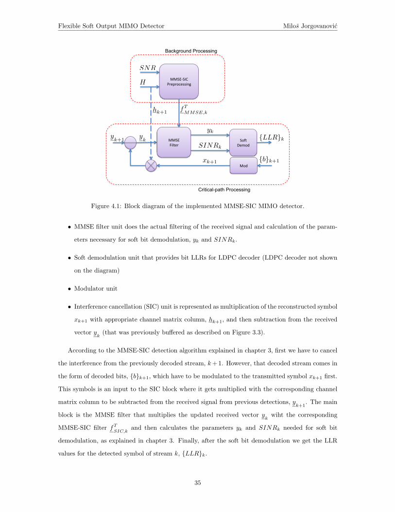
Compared to the conceptual MMSE-SIC detector block diagram shown on Figure 3.3, the actual
implementation is slightly different. Figure 4.1 presents the architecture block diagram with main
signals denoted. We notice the following blocks:
• MMSE-SIC preprocessing unit calculates the filter coefficients using the square-root algorithm.
This block is typically not time critical, assuming the channel is not changing very fast (i.e.
assuming the channel is relatively slow-fading), however we have taken into account the possible
extension to multi-carrier system in which many channel instances would have to be processed
at the same time and the architecture is pipelined so it can be easily extended to support that.
34
Flexible Soft Output MIMO Detector Milos Jorgovanovic
So# Demod
MMSE-‐SIC Preprocessing
MMSE Filter
Mod
fT
MMSE,k
H
hk+1
yk
SINRk
xk+1 {b}k+1
{LLR}k
SNR
Background Processing
Critical-path Processing
yk+1
yk
Figure 4.1: Block diagram of the implemented MMSE-SIC MIMO detector.
• MMSE filter unit does the actual filtering of the received signal and calculation of the param-
eters necessary for soft bit demodulation, yk and SINRk.
• Soft demodulation unit that provides bit LLRs for LDPC decoder (LDPC decoder not shown
on the diagram)
• Modulator unit
• Interference cancellation (SIC) unit is represented as multiplication of the reconstructed symbol
xk+1 with appropriate channel matrix column, hk+1, and then subtraction from the received
vector yk
(that was previously buffered as described on Figure 3.3).
According to the MMSE-SIC detection algorithm explained in chapter 3, first we have to cancel
the interference from the previously decoded stream, k+ 1. However, that decoded stream comes in
the form of decoded bits, {b}k+1, which have to be modulated to the transmitted symbol xk+1 first.
This symbols is an input to the SIC block where it gets multiplied with the corresponding channel
matrix column to be subtracted from the received signal from previous detections, yk+1
. The main
block is the MMSE filter that multiplies the updated received vector yk
wiht the corresponding
MMSE-SIC filter fTSIC,k
and then calculates the parameters yk and SINRk needed for soft bit
demodulation, as explained in chapter 3. Finally, after the soft bit demodulation we get the LLR
values for the detected symbol of stream k, {LLR}k.
35

Flexible Soft Output MIMO Detector Milos Jorgovanovic
Notice that compared to the diagram on Figure 3.3, chosen architecture has only one critical
path ”branch” that consists of MMSE filter block, soft demodulator, modulator and SIC block. Of
course, it would be straightforward to add more branches and parallelize the computation which
would directly increase the throughput, but even with only one branch we can still meet the LTE
standard requirements. According to design philosophy of reducing the hardware resources as much
as possible, we have decided to have only one MMSE filter + SIC branch which is pipelined for
maximum performance.
The hardware design is done using MATLAB Simulink and building blocks from the Xilinx
library. This means that the main purpose of this design is to be implemented on Xilinx FPGA
chip, since it uses some of the special features it has to offer, like embedded Multiply and ACcuulate
(MAC) units or embedded RAM blocks (DSP48 and BRAM, respectively). It can however be
translated to Verilog or VHDL, but then these embedded FPGA blocks would have to be designed
separately.
In the rest of this chapter, we pay most of the attention to the implementation of the preprocessing
unit that calculates the MMSE-SIC filter coefficients based on the square-root algorithm. Specifically,
we explain in detail how the unitary operation Θi from equation (3.31) is done in hardware without
any matrix multiplications, by using the systolic array architecture and CORDIC algorithm for
implementation. Then we turn to the actual MMSE filtering and soft bit demodulation the way it
was explained in the last two sections of chapter 3. These blocks are on the critical path of the design
and they are optimized to meet the throughput requirements given by the LTE standard. Another
two blocks take care of the interference cancellation - modulator that modulates decoded bits back
to the transmitted symbols and the actual SIC block that subtracts their influence from the received
vector as shown by equation (3.12). Finally, the chapter is concluded with the speed and resource
utilization results obtained through synthesizing the design for an FPGA implementation.
4.1 Implementation of the Systolic Array
The central part in the preprocessing unit is the row nulling operation given by (3.31). The main idea
of nulling the row is to use one column as so called pivot, and apply series of unitary transformations
(matrix rotations) that will keep changing only the pivot and the targeted column, until the first
(leading) element of the targeted column is nulled [14]. In general, matrix elements are complex (we
are dealing with the complex channel and the complex constellation), but the very first element in
the row we are trying to null will indeed always be real. Namely, in expression (3.31) this is obvious
36

Flexible Soft Output MIMO Detector Milos Jorgovanovic
since the first element in the first row is 1 in every iteration. Let us first show how we null one
complex element of the first row, without changing the other ones.
4.1.1 Nulling a Single Element in a Row
Let’s assume we want to null the i-th element of the first row (c1,i), by using the first column as a
pivot. In general, this element is a complex number, and the first step is to null its imaginary part.
In order to do this, we can represent the complex number in Euler form:
c1,i = r1,iejθ1,i . (4.1)
It is easy to see that we can rotate this complex number to align with the real axis by multiplying
it with e−jθ1,i . However, the goal is to keep applying only unitary operations on the given matrix,
and in order to do so, we have to multiply the whole i-th column with the same number. This
operation is given by Qθi (4.2), which is identity matrix with i-th diagonal element replaced by
ejθi = e−jθ1,i .
Qθi =
1 0 . . . 0 . . . 0
0 1 . . . 0 . . . 0...
.... . .
... . . ....
0 0 . . . ejθi . . . 0...
... . . ....
. . ....
0 0 . . . 0 . . . 1
. (4.2)
The multiplication of the original matrix with this one now results in (4.3), where ’r’ is used to
denote that the particular matrix element is real and ’c’ is used for (in general) complex elements.
r1,1 . . . c1,i . . .
c2,1 . . . c2,i . . .
... . . .... . . .
cn,1 . . . cn,i . . .
Qθi =
r1,1 . . . r1,i . . .
c2,1 . . . c′2,i . . .
... . . .... . . .
cn,1 . . . c′n,i . . .
. (4.3)
To null the real element of the matrix, we use another type of unitary transformation called
a Givens transformation, Qφi . This transformation is derived again from the identity matrix, by
changing four elements, as given by (4.4).
37
Flexible Soft Output MIMO Detector Milos Jorgovanovic
Qφi =
cosφi 0 . . . sinφi . . . 0
0 1 . . . 0 . . . 0...
.... . .
... . . ....
− sinφi 0 . . . cosφi . . . 0...
... . . ....
. . ....
0 0 . . . 0 . . . 1
(4.4)
When we postmultiply with Qφi , we only affect the first and the i-th column. Given that the
elements of the first row in these two columns were r1,1 and r1,i, after Givens transformation we will
have:
r1,1 . . . r1,i . . .
c2,1 . . . c′2,i . . .
... . . .... . . .
cn,1 . . . c′n,i . . .
Qφi =
r′1,1 . . . 0 . . .
c′2,1 . . . c
′′2,i . . .
... . . .... . . .
c′n,1 . . . c
′”n,i . . .
, (4.5)
where
r′1,1 = r1,1 cosφi − r1,i sinφi
0 = r1,i cosφi + r1,1 sinφi.(4.6)
Note that since the transformation is real, the leading element of the updated pivot column (r′1,1)
stays real. This implies that the updated pivot column can be reused as a pivot column for nulling
the next element of the first row. Now we can summarize how we choose the two unitary operations
needed to null the i-th element of the first row:
• For nulling the imaginary part by using Qθi (4.2), we have to determine the angle θi based on
the argument of the i-th element in the first row:
θi = −θ1,i = − arg{c1,i} = arctan(−imag{c1,i}
real{c1,i}
)(4.7)
If we look into the mechanics of this unitary transformation (4.3), we notice that it changes
only the i-th column. If we further break the complex elements of the i-th column into the real
and imaginary parts, the transformation (applied only to this column, since other columns do
not change) takes the form:
38

Flexible Soft Output MIMO Detector Milos Jorgovanovic
Real{c1,i} Imag{c1,i}
Real{c2,i} Imag{c2,i}...
...
Real{cn,i} Imag{cn,i}
cos θi sin θi
− sin θi cos θi
(4.8)
• For nulling the real part by using Qφi (4.4) we have to determine the angle φi based on (4.6)
as:
φi = arctan(−r1,ir1,1
)(4.9)
Looking into this unitary transformation(4.4), we notice that the transformation itself is real,
meaning that we can separately process the real and imaginary part in expression (4.5). Iso-
lating the effect on the first and the i-th columns (the others are not affected), we get that for
real parts the transformation takes the form:
Real{c1,1} Real{c1,i}
Real{c2,1} Real{c2,i}...
...
Real{cn,1} Real{cn,i}
cosφi sinφi
− sinφi cosφi
. (4.10)
Exactly the same expression holds for the imaginary parts.
Now we can conclude that the two unitary transformations are essentially of the same form. The
only difference is that Qθi is applied to the two columns being the real and imaginary parts of the
column i whose leading element we want to null. Transformation Qφi on the other hand has to be
applied twice, to the real parts of the first and the i-th column, as well as to their imaginary parts.
So, we have managed to null the i-th element of the first row by applying two simple unitary
operations and changing only the elements of the first and the i-th column. This is very important
since it promises low complexity implementation - only two columns are involved, not the whole
matrix. Of course, in order to null the whole row, we have to repeat these two operation for each
element of the first row.
39
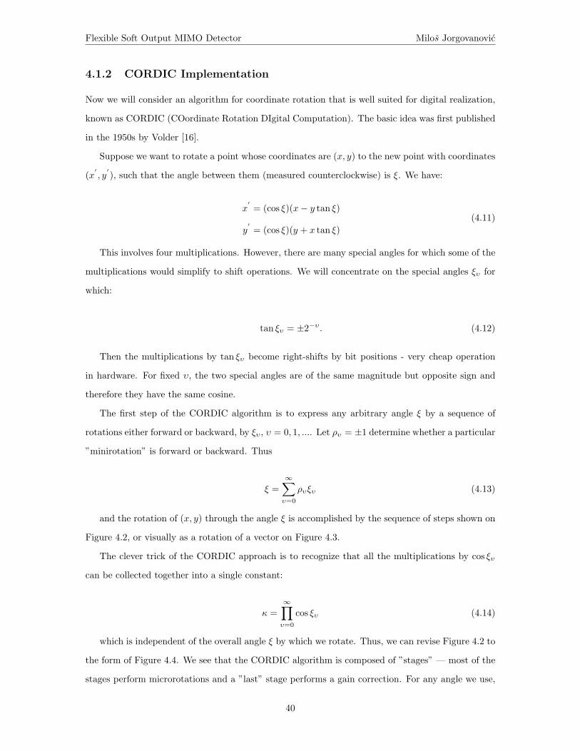
Flexible Soft Output MIMO Detector Milos Jorgovanovic
4.1.2 CORDIC Implementation
Now we will consider an algorithm for coordinate rotation that is well suited for digital realization,
known as CORDIC (COordinate Rotation DIgital Computation). The basic idea was first published
in the 1950s by Volder [16].
Suppose we want to rotate a point whose coordinates are (x, y) to the new point with coordinates
(x′, y
′), such that the angle between them (measured counterclockwise) is ξ. We have:
x′
= (cos ξ)(x− y tan ξ)
y′
= (cos ξ)(y + x tan ξ)(4.11)
This involves four multiplications. However, there are many special angles for which some of the
multiplications would simplify to shift operations. We will concentrate on the special angles ξυ for
which:
tan ξυ = ±2−υ. (4.12)
Then the multiplications by tan ξυ become right-shifts by bit positions - very cheap operation
in hardware. For fixed υ, the two special angles are of the same magnitude but opposite sign and
therefore they have the same cosine.
The first step of the CORDIC algorithm is to express any arbitrary angle ξ by a sequence of
rotations either forward or backward, by ξυ, υ = 0, 1, .... Let ρυ = ±1 determine whether a particular
”minirotation” is forward or backward. Thus
ξ =∞∑
υ=0
ρυξυ (4.13)
and the rotation of (x, y) through the angle ξ is accomplished by the sequence of steps shown on
Figure 4.2, or visually as a rotation of a vector on Figure 4.3.
The clever trick of the CORDIC approach is to recognize that all the multiplications by cos ξυ
can be collected together into a single constant:
κ =∞∏
υ=0
cos ξυ (4.14)
which is independent of the overall angle ξ by which we rotate. Thus, we can revise Figure 4.2 to
the form of Figure 4.4. We see that the CORDIC algorithm is composed of ”stages” — most of the
stages perform microrotations and a ”last” stage performs a gain correction. For any angle we use,
40
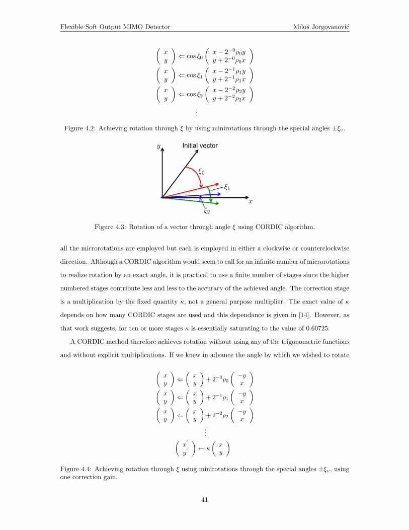
Flexible Soft Output MIMO Detector Milos Jorgovanovic
�xy
�⇐ cos ξ0
�x− 2−0ρ0yy + 2−0ρ0x
�
�xy
�⇐ cos ξ1
�x− 2−1ρ1yy + 2−1ρ1x
�
�xy
�⇐ cos ξ2
�x− 2−2ρ2yy + 2−2ρ2x
�
...
Figure 4.2: Achieving rotation through ξ by using minirotations through the special angles ±ξυ.
x
y Initial vector
ξ0
ξ1
ξ2
Figure 4.3: Rotation of a vector through angle ξ using CORDIC algorithm.
all the microrotations are employed but each is employed in either a clockwise or counterclockwise
direction. Although a CORDIC algorithm would seem to call for an infinite number of microrotations
to realize rotation by an exact angle, it is practical to use a finite number of stages since the higher
numbered stages contribute less and less to the accuracy of the achieved angle. The correction stage
is a multiplication by the fixed quantity κ, not a general purpose multiplier. The exact value of κ
depends on how many CORDIC stages are used and this dependance is given in [14]. However, as
that work suggests, for ten or more stages κ is essentially saturating to the value of 0.60725.
A CORDIC method therefore achieves rotation without using any of the trigonometric functions
and without explicit multiplications. If we knew in advance the angle by which we wished to rotate
�xy
�⇐
�xy
�+ 2−0ρ0
�−yx
�
�xy
�⇐
�xy
�+ 2−1ρ1
�−yx
�
�xy
�⇐
�xy
�+ 2−2ρ2
�−yx
�
...�
x�
y�
�← κ
�xy
�
Figure 4.4: Achieving rotation through ξ using minirotations through the special angles ±ξυ, usingone correction gain.
41
Flexible Soft Output MIMO Detector Milos Jorgovanovic
the pair (x, y), we could determine the set of controls (ρυ, υ = 0, 1, ..., υmax), each represented by a
single bit.
However, in the present application we do not know the angle of rotation in advance. We are
given a pair (x, y) and we must rotate that pair through the angle such that the resulting rotated
pair takes the form (x′, 0). This operation is called vectoring. Then we have to rotate some number
of other pairs through the same angle. We have no need to actually know what the angle is, as
long as we are able to rotate by that angle. This operation is called rotating. For vectoring followed
by rotating what we really need is an algorithm to determine the CORDIC controls ρυ. A major
advantage of the CORDIC algorithm is that the same circuit which is used for vectoring may be
used for rotating.
Consider just the first CORDIC stage, for which the special angle is either 45◦ or −45◦. Since
our purpose is to rotate the input (x, y) toward the x axis, if y is ”above” the x axis we should rotate
”down” and if y is ”below” the x axis we should rotate ”up”, Figure 4.3. The angular direction of
”down” is also dependent on whether x is positive or negative (if either x or y is zero, we can choose
any direction). Therefore,
ρ0 = sgn(x)sgn(y). (4.15)
Once we have determined ρ0, we compute the effect of the first stage on x and y and pass the
modified (x, y) to the second stage. Here, again, our rule is to rotate ”down” if y is ”above” the x
axis and ”up” if it is ”below” the x axis:
ρ1 = sgn(x)sgn(y). (4.16)
In this way, the determination of the controls is quite simple:
ρυ = sgn(x)sgn(y), υ = 0, 1, ..., υmax (4.17)
These controls, once determined, are saved in the flip-flops of the specialized stages and used to
control those stages for the succeeding (x, y) pairs which are to be rotated through the same angle.
In Figure 4.5 we show the concept of a CORDIC circuit made up of independent stages. The
inputs (x, y) are modified by minirotations as they proceed from stage to stage. This circuit has
the virtue of natural pipelining. If registers are placed between the stages, then a new rotation
problem, involving a new pair (x, y), can be started by the circuit as soon as the preceding pair has
42
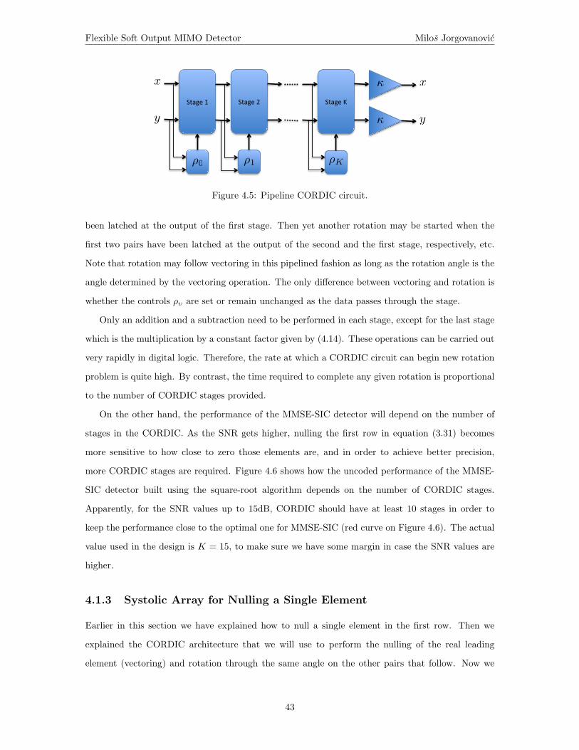
Flexible Soft Output MIMO Detector Milos Jorgovanovic
Stage 2 Stage K Stage 1
x
y
x
y
ρ0 ρ1 ρK
κ
κ
Figure 4.5: Pipeline CORDIC circuit.
been latched at the output of the first stage. Then yet another rotation may be started when the
first two pairs have been latched at the output of the second and the first stage, respectively, etc.
Note that rotation may follow vectoring in this pipelined fashion as long as the rotation angle is the
angle determined by the vectoring operation. The only difference between vectoring and rotation is
whether the controls ρυ are set or remain unchanged as the data passes through the stage.
Only an addition and a subtraction need to be performed in each stage, except for the last stage
which is the multiplication by a constant factor given by (4.14). These operations can be carried out
very rapidly in digital logic. Therefore, the rate at which a CORDIC circuit can begin new rotation
problem is quite high. By contrast, the time required to complete any given rotation is proportional
to the number of CORDIC stages provided.
On the other hand, the performance of the MMSE-SIC detector will depend on the number of
stages in the CORDIC. As the SNR gets higher, nulling the first row in equation (3.31) becomes
more sensitive to how close to zero those elements are, and in order to achieve better precision,
more CORDIC stages are required. Figure 4.6 shows how the uncoded performance of the MMSE-
SIC detector built using the square-root algorithm depends on the number of CORDIC stages.
Apparently, for the SNR values up to 15dB, CORDIC should have at least 10 stages in order to
keep the performance close to the optimal one for MMSE-SIC (red curve on Figure 4.6). The actual
value used in the design is K = 15, to make sure we have some margin in case the SNR values are
higher.
4.1.3 Systolic Array for Nulling a Single Element
Earlier in this section we have explained how to null a single element in the first row. Then we
explained the CORDIC architecture that we will use to perform the nulling of the real leading
element (vectoring) and rotation through the same angle on the other pairs that follow. Now we
43

Flexible Soft Output MIMO Detector Milos Jorgovanovic
Figure 4.6: Uncoded MMSE-SIC detector performance versus number of stages in CORDIC.
will put these pieces together and present the complete architecture for nulling a complex element
of the first row.
To null the complex part of the first element in the targeted column, we have to perform the Qθ
transformation given by (4.8). We will assign one CORDIC circuit to perform this transformation.
Next, (4.10) explains how Qφ transformation is performed. This transformation has to be applied
to the two complex columns (the first one and the i-th one), but since the operation is real it can
be applied separately to the real and imaginary parts of these two columns. This means that in
order to process the two complex columns we need to assign two CORDIC circuits to perform this
operation.
Data, in the form of columns of complex numbers, are presented to the circuitry sequentially. and
the time during which one complex word enters a CORDIC block will bi called a microcycle. Every
column that enters a circuit will have a leader, its first element, and some number of followers, all
the other elements in the column. The CORDIC block performs vectoring on the leader and rotation
through the same angle for the followers. A column composed of, say, K elements will flow into a
CORDIC circuit during K consecutive microcycles. The elements making up such a column will flow
44

Flexible Soft Output MIMO Detector Milos Jorgovanovic
Master φ -‐ CORDIC
Slave φ -‐ CORDIC
θ -‐ CORDIC
Re{c1}
Re{ci}
Im{ci}
Im{c1}
Im{c�1}
Im{c�i}
Re{c�i}
Re{c�1}
Figure 4.7: CORDIC Super Cell block.
out of the CORDIC circuit at the same rate they entered, one element per microcycle. Although the
elements are modified by passing through the CORDIC block they retain their identity and their
order, and the leader on input remains the leader at the output.
The Qθ transformation is simply the passage of the i-th column of complex numbers (ci) through
a CORDIC block. The action of the CORDIC block on the leader is a phase change such that the
leader becomes real. The action of the CORDIC circuit on the followers is to change their phases
by the same amount. A CORDIC circuit used in this manner will be called a θ-CORDIC (Figure
4.7).
The Qφ transformation is a rotation of two columns of complex numbers through a real angle.
To accomplish a Qφ transformation we use two CORDIC blocks, which we shall call the master φ-
CORDIC and the slave φ-CORDIC. The master φ-CORDIC deals with real parts of columns c1 and
ci, while the slave φ-CORDIC deals with their imaginary parts, as presented on Figure 4.7. Data
involved in a Qφ transformation are presented to the two φ-CORDICs as two separate columns of
”complex” elements so that the rotation may be accomplished as if it were a phase change, by using
the equivalency of the two transformations, (4.8) and (4.10).
The master φ-CORDIC gets its two inputs from the real parts of the two columns, c1 and ci.
The first pair of inputs (Re{c1,1},Re{c1,i}) is marked as the leader, and as it passes through the
master φ-CORDIC it determines the angle controls ρυ for that CORDIC, which are to be used to
rotate all the following pairs of elements of the real parts of these two columns. However, the same
angle should be used in the slave φ-CORDIC to rotate the imaginary parts of these two columns.
Here we recall that the leading elements of both the pivot column (c1) and the targeted column (ci)
are real - the former being real due to the nature of the square-root algorithm (3.31) and the latter
due to passing through the θ-CORDIC that nulled the imaginary part of the leading element of ci.
45

Flexible Soft Output MIMO Detector Milos Jorgovanovic
This means that the leading pair of the slave φ-CORDIC is going to be (0, 0) and so it is going to
stay (0, 0) at the output as well. Thus, instead of feeding the slave φ-CORDIC with (0, 0), we can
feed the same leading pair as to the master φ-CORDIC and just ignore the leading element at the
output (pick (0, 0) instead). This way, all the pairs of the imaginary parts of the columns c1 and
ci are going to be rotated through the same angle as the real parts in the master φ-CORDIC —
exactly what we initially wanted.
In this way, the use of three CORDIC blocks accomplishes the pair of transformation needed to
zero out one element in the targeted column, ci. We call this configuration the Super Cell block.
Note that the outputs of the two φ-CORDICs have to be reassembled. The real parts of the φ-
CORDICs become the real and imaginary parts respectively of the updated pivot column, c′1. The
imaginary parts of the φ-CORDIC outputs become the real and imaginary parts respectively of the
updated targeted column, c′i, as presented on Figure 4.7. For simplicity of the Super Cell block
diagram, the multiplexing that happens at the input and the output of the slave φ-CORDIC block
is not shown.
4.1.4 Nulling the Row of the Matrix
Finally, on Figure 4.8 we present the complete circuitry that performs nulling the row of the matrix
(except, of course, the leading element of the pivot column). The central part is the Super Cell block
that performs nulling of a single elements. The operation starts by loading the matrix elements in
the Read Mem block on Figure 4.8. Next, in the first iteration we feed the Super Cell block with
the first column (c1) as the pivot and the second column (c2) as the target. The targeted column at
the output is stored in the Write Mem block as the second column of the resulting matrix (its first
element being nulled). The updated pivot column at the output of the Super Cell block however, has
to be reused as the pivot for the second iteration when we target the third column of the matrix, c3.
Thus, the next target column, c3, will be fed to the Super Cell block such that it gets aligned with
the updated pivot column from the first iteration. Note that the leading element of the updated
pivot column stays real, as shown in equation (4.6). The iterations continue in the same fashion,
until all the columns have been targeted and their leading elements nulled. Finally, we read the
Write Mem block that now has the updated matrix stored, and provide the output which has the
whole first row (except for the first element) nulled.
Block diagram shown on Figure 4.8 does not present all control signals for simplicity, but the im-
plemented block allows nulling the first row of any complex matrix (M×N) up to size of 31x16. Dur-
46
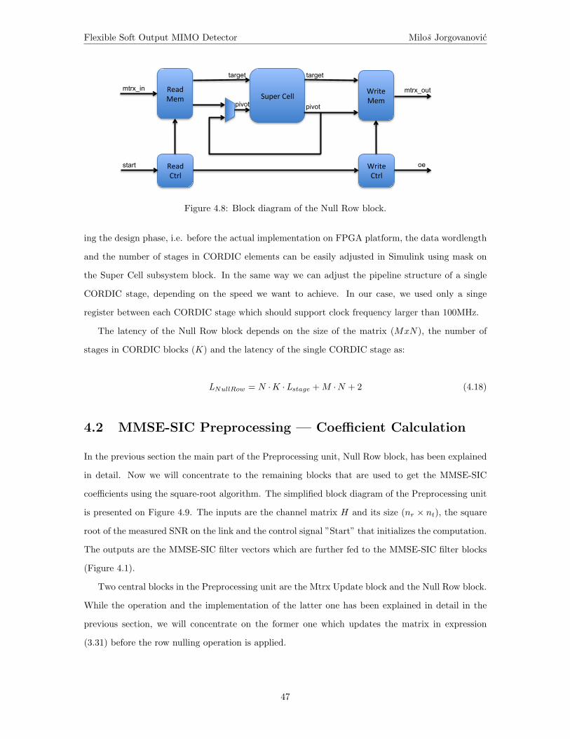
Flexible Soft Output MIMO Detector Milos Jorgovanovic
Super Cell Read Mem
Write Mem
Read Ctrl
Write Ctrl
target
pivot pivot
target
mtrx_in mtrx_out
start oe
Figure 4.8: Block diagram of the Null Row block.
ing the design phase, i.e. before the actual implementation on FPGA platform, the data wordlength
and the number of stages in CORDIC elements can be easily adjusted in Simulink using mask on
the Super Cell subsystem block. In the same way we can adjust the pipeline structure of a single
CORDIC stage, depending on the speed we want to achieve. In our case, we used only a singe
register between each CORDIC stage which should support clock frequency larger than 100MHz.
The latency of the Null Row block depends on the size of the matrix (MxN), the number of
stages in CORDIC blocks (K) and the latency of the single CORDIC stage as:
LNullRow = N ·K ·Lstage +M ·N + 2 (4.18)
4.2 MMSE-SIC Preprocessing — Coefficient Calculation
In the previous section the main part of the Preprocessing unit, Null Row block, has been explained
in detail. Now we will concentrate to the remaining blocks that are used to get the MMSE-SIC
coefficients using the square-root algorithm. The simplified block diagram of the Preprocessing unit
is presented on Figure 4.9. The inputs are the channel matrix H and its size (nr × nt), the square
root of the measured SNR on the link and the control signal ”Start” that initializes the computation.
The outputs are the MMSE-SIC filter vectors which are further fed to the MMSE-SIC filter blocks
(Figure 4.1).
Two central blocks in the Preprocessing unit are the Mtrx Update block and the Null Row block.
While the operation and the implementation of the latter one has been explained in detail in the
previous section, we will concentrate on the former one which updates the matrix in expression
(3.31) before the row nulling operation is applied.
47
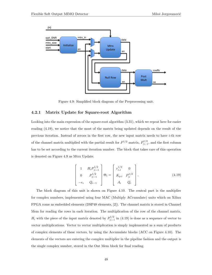
Flexible Soft Output MIMO Detector Milos Jorgovanovic
Mtrx Update
en
data mtrx_in
en
Null Row en
data
Ini4alize
coeffs
oe
Post Mult
sqrt_SNR
mtrx_size
start
{H}
Figure 4.9: Simplified block diagram of the Preprocessing unit.
4.2.1 Matrix Update for Square-root Algorithm
Looking into the main expression of the square-root algorithm (3.31), which we repeat here for easier
reading (4.19), we notice that the most of the matrix being updated depends on the result of the
previous iteration. Instead of zeroes in the first row, the new input matrix needs to have i-th row
of the channel matrix multiplied with the partial result for P 1/2 matrix, P 1/2|i−1, and the first column
has to be set according to the current iteration number. The block that takes care of this operation
is denoted on Figure 4.9 as Mtrx Update.
1 HiP1/2|i−1
0 P1/2|i−1
−ei Qi−1
Θi =
r1/2e,i 0
Kp,i P1/2|i
Ai Qi
, (4.19)
The block diagram of this unit is shown on Figure 4.10. The central part is the multiplier
for complex numbers, implemented using four MAC (Multiply ACcumulate) units which on Xilinx
FPGA come as embedded elements (DSP48 elements, [2]). The channel matrix is stored in Channel
Mem for reading the rows in each iteration. The multiplication of the row of the channel matrix,
Hi with the piece of the input matrix denoted by P 1/2|i−1 in (4.19) is done as a sequence of vector to
vector multiplications. Vector to vector multiplication is simply implemented as a sum of products
of complex elements of these vectors, by using the Accumulate blocks (ACC on Figure 4.10). The
elements of the vectors are entering the complex multiplier in the pipeline fashion and the output is
the single complex number, stored in the Out Mem block for final reading.
48
Flexible Soft Output MIMO Detector Milos Jorgovanovic
This buffering at the output is necessary since different parts of the updated matrix are ready
at different times. The first column is initialized just by knowing the current iteration, the first row
(except for the first element) has to be calculated by multiplication of the complex vector with the
complex matrix as explained, and the rest of the updated matrix is just propagated from the input
(4.19).
4.2.2 Final Remarks on the Implementation of Preprocessing Unit
Going back to the block diagram of the Preprocessing unit on Figure 4.9 and referring to the square-
root algorithm explained through (3.31) or (4.19), it can be concluded that one iteration of (4.19)
consists of one matrix update operation and one row nulling. That means that after the initialization
of the matrix that is going to be iterated in (4.19), which is done in Initialize block on Figure 4.9,
we have to iterate nr times between the Mtrx Update and Null Row blocks, as shown on the block
diagram. Finally, after nr iterations we have the desired matrices P 1/2 and Qα. The only step left
is to get the exact MMSE-SIC filter coefficients by post-multiplying columns of the Qα matrix with
the corresponding diagonal values of P 1/2 matrix, as suggested by (3.30).
Finally, we also show the complete block diagram of the Preprocessing unit as a screenshot of
the Simulink design, Figure 4.11. We can identify the main building blocks to be the same as on
the simplified diagram from Figure 4.9.
4.3 Critical Path
In the previous section we have explained the design of the Preprocessing unit, which we refer to as
a background processing, as denoted on Figure 4.1. It is called background since MMSE-SIC filter
coefficients are calculated only when the MIMO channel changes significantly from the previous
value, which is in general happening every coherence time (Tc) interval, typically the value of 1ms
or larger. Critical path processing on the other hand happens every time the new signal y is received,
which in practical implementation usually means continuously. Thus, in order to speed up the data
processing and increase the throughput of the whole MIMO detector, it is very important to design
the critical path to be fast enough.
Luckily, the blocks on the critical path are fairly simple and can be made very fast by pipelining.
In the remaining of this section we will briefly explain the implementation of each of these blocks.
49

Flexible Soft Output MIMO Detector Milos Jorgovanovic
MAC
First
column
iter
star
t
inpu
t_m
trx
{H}
Channe
l Mem
“0”
X
+
MAC
“0” +
MAC
+
MAC
+
Out
Mem
ACC
ACC
split
Re
Im
Re
Im
-‐Z-‐1
Z-‐1
Re Im
con
cat
Read
Ctrl 1
iter
star
t
Read
Ctrl 2
Com
plex
Mul
tiplic
atio
n ite
r
star
t
mtrx
_out
oe
X
X
X
Z-‐1
Figure 4.10: Block diagram of the Mtrx Update unit.
50

Flexible Soft Output MIMO Detector Milos Jorgovanovic
Figure 4.11: Screenshot of the Preprocessing unit design in Simulink51

Flexible Soft Output MIMO Detector Milos Jorgovanovic
Figure 4.12: Screenshot of the Modulator unit design in Simulink.
4.3.1 Modulator
The function of the modulator block is to translate coded bits into the transmit symbols. The most
straightforward implementation is using the LookUp Table (LUT), where Gray mapping for LTE
standard is used. From the Simulink screenshot presented on Figure 4.12 it can be noticed that
there is a separate LUT for each constellation - this is the case since all of these LUTs have been
implemented as distributed memory on the FPGA chip.
4.3.2 SIC
As previously indicated, the function of SIC block is to cancel the interference of the decoded
transmitted symbol. This complex symbol xk+1 has to be multiplied by k+1-st channel column and
then subtracted from the received signal yk+1
. Block diagram of the SIC unit has been implemented
on Figure 4.13.
Note that the the whole computation chain is registered after each add or multiply operation.
This block is fully pipelined in terms of the received signal yk+1
, assuming that decoded transmit
symbols xk+1 arrive aligned with it.
52

Flexible Soft Output MIMO Detector Milos Jorgovanovic
MAC
stream
en
{H} Channel Mem
“0”
X
+
MAC
“0”
+
MAC +
MAC +
split
Re
Im
Re
Im
-‐Z-‐1
Z-‐1
Re
Im
concat Read
Ctrl 1
Complex Multiplication
X
X
X
split Re
Im
-
-
Z-‐3
Z-‐2
Z-‐2
oe
yk
yk+1
xk+1
Z-‐1
Figure 4.13: Block diagram of the interference cancellation unit.
4.3.3 MMSE-SIC Filter
MMSE-SIC block has to perform filtering of the received signal yk, by multiplying it with the
MMSE-SIC vector, fSIC,k
. For this we again use the complex multiplication block from the previous
diagrams, with accumulators behind, Figure 4.14. In order to calculate the SINRk value as explained
in chapter 3, we have to filter the channel column itself with the same fitler and then perform x/(1−x)
function, (3.51). Note that in this case we care only about the real part of the filtering operation,
since the SINR is the real number.
Also, from (3.54) we have concluded that we can use the same x/(1−x) type LUT for calculating
the received symbol yk that we further process in the soft demodulation block. Thus, the outputs
of the MMSE-SIC Filter block are the inputs to the Soft Demodulator block, yk and SINRk.
This block is also fully pipelined in terms of the received vector yk, i.e. these vectors can enter
the block immediately one after another.
4.3.4 Soft Bit Demodulator
The last block on the critical path is the Soft Bit Demodulator block that uses the received symbol yk
and the SINR of that stream, SINRk, to calculate the LLRs of the demodulated bits. The technique
used here is again based on the LUT, since we have concluded that it can provide significant reduction
53
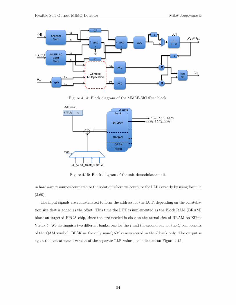
Flexible Soft Output MIMO Detector Milos Jorgovanovic
Complex Multiplication
Channel Mem
MMSE-‐SIC Coeff Mem
ACC
ACC
Re
Im
Re
Im
Re
Im
split
Re
Im
MAC
“0”
X
+
MAC
-‐Z-‐1
X
Z-‐1
ACC x
1−x
LUT -‐1
+1
X
X
concat
+
yk
{H}
fSIC,k
SINRk
yk
Figure 4.14: Block diagram of the MMSE-SIC filter block.
64-QAM
16-QAM
QPSK
BPSK
Address: Q bank
LLR1, LLR3, LLR5
LLR2, LLR4, LLR6
mod
off_64 off_16 off_4 off_2
64-QAM
16-QAM
QPSK
BPSK
I bank SINRk yk
Figure 4.15: Block diagram of the soft demodulator unit.
in hardware resources compared to the solution where we compute the LLRs exactly by using formula
(3.60).
The input signals are concatenated to form the address for the LUT, depending on the constella-
tion size that is added as the offset. This time the LUT is implemented as the Block RAM (BRAM)
block on targeted FPGA chip, since the size needed is close to the actual size of BRAM on Xilinx
Virtex 5. We distinguish two different banks, one for the I and the second one for the Q components
of the QAM symbol. BPSK as the only non-QAM case is stored in the I bank only. The output is
again the concatenated version of the separate LLR values, as indicated on Figure 4.15.
54
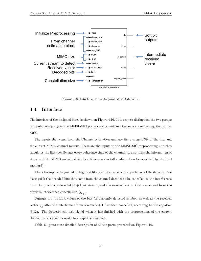
Flexible Soft Output MIMO Detector Milos Jorgovanovic
From channel estimation block
MIMO size
Current stream to detect Received vector
Decoded bits
Constellation size
Initialize Preprocessing Soft bit outputs
Intermediate received vector
Figure 4.16: Interface of the designed MIMO detector.
4.4 Interface
The interface of the designed block is shown on Figure 4.16. It is easy to distinguish the two groups
of inputs: one going to the MMSE-SIC preprocessing unit and the second one feeding the critical
path.
The inputs that come from the Channel estimation unit are the average SNR of the link and
the current MIMO channel matrix. These are the inputs to the MMSE-SIC preprocessing unit that
calculates the filter coefficients every coherence time of the channel. It also takes the information of
the size of the MIMO matrix, which is arbitrary up to 4x8 configuration (as specified by the LTE
standard).
The other inputs designated on Figure 4.16 are inputs to the critical path part of the detector. We
distinguish the decoded bits that come from the channel decoder to be cancelled as the interference
from the previously decoded (k + 1)-st stream, and the received vector that was stored from the
previous interference cancellation, yk+1
.
Outputs are the LLR values of the bits for currently detected symbol, as well as the received
vector yk
after the interference from stream k + 1 has been cancelled, according to the equation
(3.12). The Detector can also signal when it has finished with the preprocessing of the current
channel instance and is ready to accept the new one.
Table 4.1 gives more detailed description of all the ports presented on Figure 4.16.
55
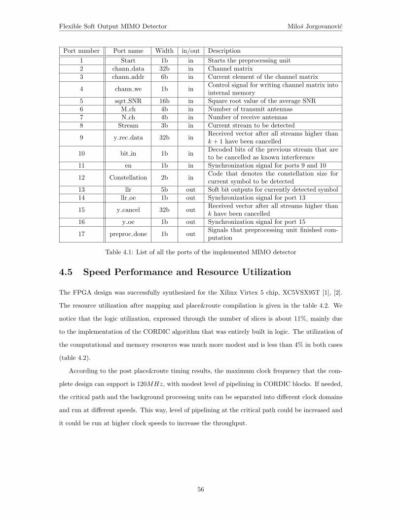
Flexible Soft Output MIMO Detector Milos Jorgovanovic
Port number Port name Width in/out Description1 Start 1b in Starts the preprocessing unit2 chann data 32b in Channel matrix3 chann addr 6b in Current element of the channel matrix
4 chann we 1b inControl signal for writing channel matrix intointernal memory
5 sqrt SNR 16b in Square root value of the average SNR6 M ch 4b in Number of transmit antennas7 N ch 4b in Number of receive antennas8 Stream 3b in Current stream to be detected
9 y rec data 32b inReceived vector after all streams higher thank + 1 have been cancelled
10 bit in 1b inDecoded bits of the previous stream that areto be cancelled as known interference
11 en 1b in Synchronization signal for ports 9 and 10
12 Constellation 2b inCode that denotes the constellation size forcurrent symbol to be detected
13 llr 5b out Soft bit outputs for currently detected symbol14 llr oe 1b out Synchronization signal for port 13
15 y cancel 32b outReceived vector after all streams higher thank have been cancelled
16 y oe 1b out Synchronization signal for port 15
17 preproc done 1b outSignals that preprocessing unit finished com-putation
Table 4.1: List of all the ports of the implemented MIMO detector
4.5 Speed Performance and Resource Utilization
The FPGA design was successfully synthesized for the Xilinx Virtex 5 chip, XC5VSX95T [1], [2].
The resource utilization after mapping and place&route compilation is given in the table 4.2. We
notice that the logic utilization, expressed through the number of slices is about 11%, mainly due
to the implementation of the CORDIC algorithm that was entirely built in logic. The utilization of
the computational and memory resources was much more modest and is less than 4% in both cases
(table 4.2).
According to the post place&route timing results, the maximum clock frequency that the com-
plete design can support is 120MHz, with modest level of pipelining in CORDIC blocks. If needed,
the critical path and the background processing units can be separated into different clock domains
and run at different speeds. This way, level of pipelining at the critical path could be increased and
it could be run at higher clock speeds to increase the throughput.
56

Flexible Soft Output MIMO Detector Milos Jorgovanovic
Resource Count Total on chip* %
Slice Registers 3,503 58,880 6.0
Slice LUTs 5,264 58,880 9.0
Slices 1,633 14,720 11.0
DSP48 Embedded MAC Units 22 640 3.4
36Kb BRAM Blocks 9 244 3.7 * FPGA chip: Xilinx Virtex5, XC5VSX95T
Table 4.2: FPGA resource utilization of the designed MIMO detector
57
Chapter 5
Conclusion
The motivation for this work is to show a practical demonstration of the cooperation between
terminals on the user side of a wireless network. The simplest setup is described - the system we
consider has one antenna at the source, one antenna at the relay and two antennas at the destination.
During the transmit phase of the relay, the destination receives two streams from the two single-
antenna transmitters, so it needs to support the MIMO reception. The central and one of the most
complex blocks of the MIMO receive baseband (Figure 2.5) is the MIMO detector. The setup we
use to prove the concept of cooperation between terminals sets certain constraints on the MIMO
system design, and further to the design of MIMO detector. This work describes the algorithm and
hardware implementation of the MIMO detector that satisfies these constraints.
We argued that MMSE-SIC is the MIMO detector architecture that represents a very good fit for
the given design requirements. The algorithm for MMSE-SIC filter calculation that promises an effi-
cient hardware implementation has been presented. The original version of this algorithm proposed
by Hassibi that has been developed for VBLAST space-time coding, was altered to accommodate
DBLAST. We have also described how to extend this algorithm to provide necessary parameters
for soft bit demodulation. It was shown that this extension can be done in a very effective way, by
using only symbol estimates (outputs of a standard MMSE-SIC MIMO detector), MMSE-SIC filter
coefficients and the channel matrix. The max-log simplification for soft bit demodulation is also
discussed and an efficient architecture is suggested.
Finally, we have also proven that the performance of this MIMO detector with all the approxi-
mations introduced is still reasonably close to the ideal MMSE-SIC performance. Figure 3.8 shows
how the designed MIMO detector performs in 2x2 MIMO system with DBLAST and LDPC coding
58

Flexible Soft Output MIMO Detector Milos Jorgovanovic
versus the ideal MMSE-SIC detector with ideal soft bit demodulation. Difference in performance is
less than 0.5dB for all QAM constellations.
Key contribution of this work is an efficient implementation of the soft output MMSE-SIC MIMO
detector for DBLAST. Using DBLAST instead of VBLAST as suggested in the original algorithm, we
manage to reduce the complexity of the preprocessing step close to 50%. Matrix inversion operations
involved in the calculation of MMSE-SIC coefficients have been avoided by using series of CORDIC
elements. To the best of our knowledge, existing algorithms and implementations of MMSE-SIC
detection do not suggest an efficient way of calculating soft bit outputs given the symbol estimates.
In this work, we have shown how soft bit outputs can be calculated with a very small computation
overhead of about 50% of the original MMSE-SIC filter block. Compared to the overall design, this
represents a negligible complexity increase. To satisfy the goal of the low hardware utilization of the
FPGA chip, the architecture has been serialized as much as the throughput requirement allowed.
Designed MIMO detector has a lot of flexibility in terms of potential use. The preprocessing
unit that calculates MMSE-SIC filter coefficients can process any MIMO channel size, up to 4 × 8
which is the current limit for LTE standard. The soft demodulator can provide soft bit outputs
for any constellation size up to 64-QAM. The interface is designed in a way that enables use of
this detector with any type of interleaving. This is possible since there is no information on the
currently processed codeword stored inside the MIMO detector. All the information that is needed
is fed through the inputs and all the information that might be needed for decoding the current
and detecting the next stream is provided at the output, for storing in external memory. The only
information that is kept internally is the average SNR and the current instance of the channel matrix.
This was done assuming the coherence time of the channel is much longer than the time needed for
the preprocessing unit to finish generating MMSE-SIC filter coefficients. We show this is a very
reasonable assumption at least for the LTE standard, where the subframe period is 0.5ms and the
time needed for calculation of MMSE-SIC coefficients is around two to three orders of magnitude
smaller.
The future work on cooperative MIMO system includes designing the source and the relay base-
band, as well as the rest of the MIMO receiver at the destination, Figure 2.5. Most challenging
blocks for implementation are synchronization, channel estimation and joint channel decoder at the
destination. The system should be preferably multi-carrier, to utilize frequency diversity and en-
able multi-user scenario both in the uplink and the downlink. Using Orthogonal Frequency-Division
Multiplexing (OFDM), which is already part of the new wireless standards (802.11n, LTE), is going
to have big impact on the channel estimation and MIMO detection blocks.
59

Flexible Soft Output MIMO Detector Milos Jorgovanovic
Proposed design of the MIMO detector can be possibly extended to the multi-carrier scenario.
Since the only information that is kept in the detector is the information about the current channel
conditions, the memory would have to be extended to accommodate the channel information about
all the subcarriers. With the small number of subcarriers, small MIMO arrays and relatively slow-
fading channel, it is be possible to extend the current design just by adding more memory and
changing memory read/write engines in MMSE-SIC preprocessing unit. This would be a brute force
solution, since no frequency correlation between channels in consecutive subcarriers is utilized. If
the channel is changing too fast or there are many channel instances to be processed (i.e. there
are many subcarriers), the design of the MIMO detector would have to be changed. The existing
architecture of MMSE-SIC preprocessing unit would have to be either parallelized, or additional
pipelining would have to be introduced in CORDIC blocks. Ideally, the MIMO detector would be
redesigned to utilize the correlation between channel gains in the consecutive subcarriers.
60
References
[1] Virtex-5 FPGA User Guide, 2010. www.xilinx.com.
[2] Virtex-5 FPGA XtremeDSP Design Considerations, 2010. www.xilinx.com.
[3] Pramod Viswanath David Tse. Fundamentals of Wireless Communication. Cambridge Univer-
sity Press, 2005.
[4] R.G. Gallager. Low-Density Parity-Check Codes. PhD thesis, MIT, 1963.
[5] M.J. Gans G.J. Foschini. On limits of wireless communications in a fading environment when
using multiple antennas. Wireless Personal Communications, 6:311–335, 1998.
[6] Z. Guo and P. Nilsson. An asic implementation for v-blast detection in 0.35 µm cmos. In Signal
Processing and Information Technology, 2004. Proceedings of the Fourth IEEE International
Symposium on, pages 95 – 98, 2004.
[7] Zhan Guo and P. Nilsson. Algorithm and implementation of the k-best sphere decoding for
mimo detection. Selected Areas in Communications, IEEE Journal on, 24(3):491 – 503, 2006.
[8] P. Gupta and P.R. Kumar. The capacity of wireless networks. Information Theory, IEEE
Transactions on, 46(2):388 –404, March 2000.
[9] B. Hassibi. An efficient square-root algorithm for blast. In Acoustics, Speech, and Signal
Processing, 2000. ICASSP ’00. Proceedings. 2000 IEEE International Conference on, volume 2,
pages II737 –II740 vol.2, 2000.
[10] Xin Jiang and Zhenghua Duan. A double-directional blast detection algorithm. In Wireless
Communications, Networking and Mobile Computing, 2005. Proceedings. 2005 International
Conference on, volume 1, pages 404 – 407, 2005.
61
Flexible Soft Output MIMO Detector Milos Jorgovanovic
[11] V. Nagpal, S. Pawar, D. Tse, and B. Nikolic. Cooperative multiplexing in the multiple an-
tenna half duplex relay channel. In Information Theory, 2009. ISIT 2009. IEEE International
Symposium on, pages 1438 –1442, jun. 2009.
[12] V. Nagpal, I. Wang, M. Jorgovanovic, D. Tse, and B. Nikolic. Quantize-map-and-forward
relaying: Coding and system design. In Forty-Eighth Annual Allerton Conference on Commu-
nication, Control, and Computing, 2010.
[13] A. Ozgur, O. Leveque, and D.N.C. Tse. Hierarchical cooperation achieves optimal capacity
scaling in ad hoc networks. Information Theory, IEEE Transactions on, 53(10):3549 –3572,
2007.
[14] C.M. Rader. Vlsi systolic arrays for adaptive nulling [radar]. Signal Processing Magazine, IEEE,
13(4):29 –49, July 1996.
[15] B. Hassibi T. Kailath, A.H. Sayed. Linear Estimation. Prentice Hall, 1999.
[16] Jack E. Volder. The cordic trigonometric computing technique. Electronic Computers, IRE
Transactions on, EC-8(3):330 –334, 1959.
[17] Yun Wang and Jinkuan Wang. Fast square-root detection algorithm for v-blast. In Wire-
less Communications, Networking and Mobile Computing, 2007. WiCom 2007. International
Conference on, pages 1340 –1343, 2007.
[18] Chia-Hsiang Yang and D. Markovic. A multi-core sphere decoder vlsi architecture for mimo
communications. In Global Telecommunications Conference, 2008. IEEE GLOBECOM 2008.
IEEE, 30 2008.
[19] Hufei Zhu, Zhongding Lei, and F.P.S. Chin. An improved square-root algorithm for blast. Signal
Processing Letters, IEEE, 11(9):772 – 775, 2004.
62