design of an autonomous intelligent demand-side management

Design of an autonomous intelligent Demand-Side Managementsystem using stochastic optimisation evolutionary algorithms

Edgar Galván-López a,n, Tom Curran b, James McDermott c, Paula Carroll c

a TAO Project, INRIA Saclay & LRI - Univ. Paris-Sud, Orsay, Franceb School of Computer Science & Statistics, Trinity College Dublin, Irelandc Management Information Systems, Lochlann Quinn School of Business, University College Dublin, Ireland

a r t i c l e i n f o

Article history:Received 2 September 2014Received in revised form10 February 2015Accepted 5 March 2015Available online 26 July 2015

Keywords:Demand-Side Management systemsEvolutionary algorithmsElectric vehiclesPeak-to-average ratioElectricity costsSmart grid time-of-use pricing

a b s t r a c t

Demand-Side Management systems aim to modulate energy consumption at the customer side of themeter using price incentives. Current incentive schemes allow consumers to reduce their costs, and fromthe point of view of the supplier play a role in load balancing, but do not lead to optimal demandpatterns. In the context of charging fleets of electric vehicles, we propose a centralised method forsetting overnight charging schedules. This method uses evolutionary algorithms to automatically searchfor optimal plans, representing both the charging schedule and the energy drawn from the grid at eachtime-step. In successive experiments, we optimise for increased state of charge, reduced peak demand,and reduced consumer costs. In simulations, the centralised method achieves improvements inperformance relative to simple models of non-centralised consumer behaviour.

& 2015 Elsevier B.V. All rights reserved.

1. Introduction

EU policy aims to reduce greenhouse gas emissions and reducedependency on imported fossil fuels. The “20–20–20” targets [1]mandate the reduction in member states to 20% below the 1990emission levels, the supply of 20% of all energy from renewableenergy sources (RESs) and a reduction in energy consumption by20% by the year 2020.

Electric vehicles (EVs) are viewed as playing a role in reducingemissions in the transport sector, but their usage causes anincrease in electricity demand. The use of RESs also causesproblems for the efficient operation of a power plant [2]. Increasedcycling (starting up and shutting down) of the power systemresults in increased wear and tear on the plant and can cause anincrease of greenhouse gas emissions.

Therefore, newmethods are required to increase electricity gridefficiency and reduce emissions. The smart grid (SG) is one mainapproach. A SG is a type of electrical power grid whose goal is torespond to the behaviour and actions of energy suppliers andconsumers to efficiently deliver economic, reliable and sustainableelectricity services. Multiple research areas have been explored inSG over recent years as a result of different challenges that have

been posed to the electrical grid. One of the most explored areas inSG is Demand-Side Management (DSM) systems as shown by theincreasing number of publications, ranging from the use ofintelligent algorithms (e.g., game theory [3], Monte Carlo-basedmethods [4], evolutionary algorithms [5], multi-agent systems [6]),real-time systems [7], up to challenges and in-depth surveys onthe area [8–11].

DSM is a set of measures to improve the energy system at theconsumer side. DSM ranges from improving energy efficiencythrough the use of better insulation or better materials up to theuse of autonomous systems to control energy resources [10]. DSMprograms include different approaches, e.g., manual conservationand energy efficiency programs [12] and Residential Load Manage-ment (RLM) [6,3]). RLM programs based on smart pricing areamongst the most popular methods.

The motivation for smart grid tariff structures is twofold. Theyallow consumers to reduce their electricity costs. At the same time,the utility company achieves a reduction in the peak-to-averageratio (PAR) in load demand resulting from the shifted consumption[6]. If no special measures are taken to avoid them, high PARvalues come about naturally because consumer electricity demandfollows a diurnal pattern, with increased load in the morning, a dipin the afternoon, a rise in the evening, and a stronger dip in themiddle of the night.

Some of these smart pricing methods are very popular. Inparticular, time-of-use (ToU) pricing has been widely adopted in some

Contents lists available at ScienceDirect

journal homepage: www.elsevier.com/locate/neucom

Neurocomputing

http://dx.doi.org/10.1016/j.neucom.2015.03.0930925-2312/& 2015 Elsevier B.V. All rights reserved.

n Corresponding author.E-mail address: [email protected] (T. Curran).

Neurocomputing 170 (2015) 270–285

www.sciencedirect.com/science/journal/09252312

www.elsevier.com/locate/neucom

http://dx.doi.org/10.1016/j.neucom.2015.03.093



http://crossmark.crossref.org/dialog/?doi=10.1016/j.neucom.2015.03.093&domain=pdf



mailto:[email protected]


European countries [11]. Other smart pricing types include critical-peak pricing, extreme day pricing, and smart grid real-time pricing.

Motivated by smart price-based approaches, we are interestedin developing an autonomous intelligent DSM system that shiftselectricity consumption of electric vehicles (EVs). To this end, weuse stochastic optimisation evolutionary algorithms (EAs). Themain contribution of this work focuses on the notion of loadshifting, borrowed from popular smart pricing-based methods. Incontrast to typical DSM approaches such as dynamic pricing,which are based on an interaction between the utility and theuser, we use a centralised approach, wherein the consumptionschedule is set centrally based on complete information of all EVs.The motivation is to achieve improvements in performance. To doso, we use EAs to automatically generate (optimal) solutions. Theuse of all EVs is considered in the solution representation used inour EAs (described in detail in Section 2). We also use this in theevaluation of candidate solutions.

To test this idea, we considered a dynamic scenario of 28simulated days, with the charging period from 18:00 to 07:30,divided into 28 time-slots of 30 min each. An action (switching EVcharging on or off) can be taken at the beginning of each time-slot.We defined three different goals:

(a) that EVs' batteries are as fully charged as possible;(b) we add an extra goal to (a) by aiming for a low fluctuation at

the transformer load (i.e., low PAR); and finally,(c) we add a third and final goal that aims to reduce electricity

costs to the consumer by using a pricing signal based on ToU.

To achieve these three goals, we propose three fitness functions.Each will be used independently in our EA and will guide ourevolutionary search to automatically create an (optimal) plan.

The core elements in this work are the following:

1. We study the impact of the representation and functionsproposed in this work when scaling the problem up (i.e., fromusing a few EVs to using dozens of them) by measuring thetransformer load, the initial and final state of charge (SoC), thePAR and electricity costs.

2. To do so, we used two EA approaches: a genetic algorithm and anevolution strategy and compared their performance against threenon-intelligent approaches (i.e., Greedy, Midnight and Randommethods), each of them simulating a specific user behaviour.

3. A dynamic scenario was used to study all these approaches byallowing having a variety of changes, i.e., different SoC for each EVfor each of the simulated days, over a 28-day simulated period.

1.1. Importance of this research in DSM

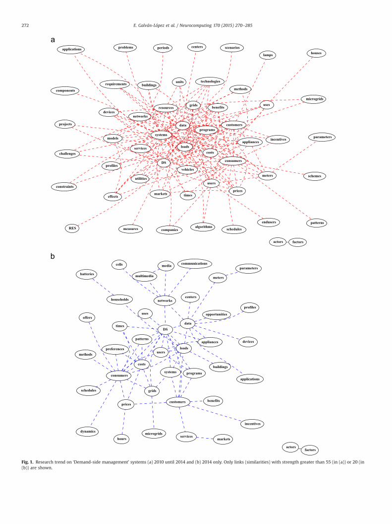
DSM has been investigated extensively over recent years. Forinstance, it has been shown that more than 2000 scientific papershave been published in this area since the 1980s [4], with morethan half in this decade. Fig. 1 shows a visual representation of theresearch trends followed in DSM (a) from 2010 until now, and(b) in 2014 only.1

As can be seen in Fig. 1 multiple topics have been covered inDSM, ranging from electricity costs, the use of electric vehicles, upto the use of data. The research conducted in this work lies at thevery core of the research trend observed in this figure.

The challenges continuously presented to the grid, such as theaggregation of new electric devices (e.g., electric vehicles using thegrid can double the average household load [3]) make the use ofintelligent algorithms suitable to be used in the design/implemen-tation of DSM systems. Fig. 1 shows this trend. For instance, noticethe presence of “algorithms”, “programs”, and “methods”. In fact,one could consider the presence of “algorithms” in the core ofFig. 1 if researchers had unified their use around this unique terminstead of using various synonyms.

Several algorithms have been used in DSM system and each hasfocused their attention on different areas within DSM. For exam-ple, it has been shown that by adopting pricing tariffs whichdifferentiate energy usage by time and level, a global optimalperformance can be achieved by means of a Nash equilibrium ofthe formulated consumption scheduling game [3]. Multi-agentsystems have also been used in DSM. For instance, the researchconducted in [14] aimed to create a DSM based on these type ofsystems and studied different types of smart pricing, concludingthat in all studied scenarios, a high PAR was observed under theuse of these smart pricing models (e.g., ToU, critical peak price,real-time pricing).

In this work we use EAs to automatically create plans tointelligently charge EVs’ batteries, aiming at reducing PAR, redu-cing load at the substation transformer, and reducing costs to theconsumer.

This paper is organised as follows. In the following section weintroduce our proposed approach. Section 3 shows the experi-mental setup used in this study. In Section 4, we present anddiscuss our findings. Section 5 draws some conclusions andpresents some future work.

2. Proposed approach

2.1. Background

Evolutionary Algorithms (EAs) [15,16], also known as Evolu-tionary Computation systems, are influenced by the theory ofevolution by natural selection. These algorithms have been with usfor some decades and are very popular due to their successfulapplication in a range of different problems, ranging from theautomated design of an antenna carried out by NASA [17], theautomated optimisation of game controllers [18,19], the auto-mated design of combinational logic circuits [20,21], to automatedoptimal localisation for building seismic sensing stations [22]. EAsare “black-box”, that is, they do not require any specific knowledgeof the fitness function. They work even when, for example, it is notpossible to define a gradient on the fitness function or to decom-pose the fitness function into a sum of per-variable objectivefunctions. The fitness functions used in our work (described inSection 2.2) are not amenable to analytic solution or simplegradient-based optimisation, hence search algorithms such asEAs are required.

The idea behind EAs is to automatically generate (nearly)optimal solutions by “evolving” potential solutions (individualsforming a population) over time (generations) by using bio-inspired operators (e.g., crossover, mutation). More specifically,the evolutionary process includes the initialisation of the popula-tion Pð0Þ at generation g¼0. The population consists of a numberof individuals which represent potential solutions to the particularproblem. At each iteration or generation (g), every individualwithin the population ðPðgÞÞ is evaluated using a fitness functionthat determines its fitness (i.e., how good or bad an individual is).Then, a selection mechanism takes place to stochastically pick thefittest individuals from the population. Some of the selectedindividuals are modified by genetic operators and the new

1 Source: http://ieeexplore.ieee.org/Xplore/home.jsp. Last accessed date: 31/08/2014. Links of strength less than 55 (in (a)) or 20 (in (b)) are filtered out. Detailson how this was produced can be found in [13].

E. Galván-López et al. / Neurocomputing 170 (2015) 270–285 271

http://ieeexplore.ieee.org/Xplore/home.jsp

algorithms

loads

users

programssystems

consumers

costs

data

networks

technologies

DS

effectsprices

units

devices

uses

requirements

vehicles

constraints

times

buildings

profiles

meters

companies

endusers

grids

customers

resources

microgrids

appliances

benefits

incentives

utilities

services

lamps

markets

challenges

scenarios

components

projects

methods

problemsapplications periods

schemes

schedules

patterns

centers

RES

models parameters

houses

measures

actors factors

grids

systemsconsumers

costs

microgrids

DS

prices

usersmethods

schedules

times

patterns

preferences

offers

dynamics

customers

loads

benefits

programs

incentives

services

data

buildings

households

appliances

applications

networks

profiles

devices

centers

opportunities

batteries

uses

meters

parameters

markets

communicationsmediacells

multimedia

hours

actorsfactors

Fig. 1. Research trend on ‘Demand-side management’ systems (a) 2010 until 2014 and (b) 2014 only. Only links (similarities) with strength greater than 55 (in (a)) or 20 (in(b)) are shown.

E. Galván-López et al. / Neurocomputing 170 (2015) 270–285272

population Pðgþ1Þ at generation gþ1 is created. The process stopswhen some halting condition is satisfied. Further details on howthese stochastic optimisation algorithms work can be found in[15,16].

2.2. Representation and evaluation

In this work, we use a fixed-length bitstring representation,where each bit indicates whether a particular EV should becharged or not during a particular time period.

Let N denote the number of household units (users). Let Mdenote the number of electric vehicles (EVs) available in N. In ourstudy M¼N. In our work the time-slots are of length 30 min,starting at ti and running to tf . Therefore an energy consumptionschedule can be naturally represented by a matrix of bits:

EM9

Eti1 ;…; Etf1Eti2 ;…; Etf2

⋮EtiM ;…; EtfM

2666664

3777775 ð1Þ

where each Etm is a single bit representing whether EV m ischarging at time t or not. Each row represents the behaviour of asingle EV over the full period; each column represents thebehaviour of all EVs at a single time-slot. An individual in the EAis just a matrix EM , unrolled to give a bitstring, that is

Eti1 ;…; Etf1 ; Eti2 ;…; Etf2 ;…; EtiM ;…; EtfM ð2Þ

Now, we need to define a fitness function (cost function) toautomatically evaluate the candidate solution shown in Eq. (2). Todo so, we need to define several elements, discussed next.

For each mAf1;…;Mg, let ltm denote the load drawn by EV m attime t. If Etm ¼ 0 then ltm ¼ 0; if Etm ¼ 1 then ltm ¼ 1:7 kW (thisconstant is characteristic of the EV). The total load across all EVsat each time tAfti;…; tf g isLt9

XmA f1;…;Mg

ltm ð3Þ

As indicated previously, we are interested in the first instancein automatically creating (near-)optimal schedules so that the finalstate of charge SoCtf for allmAf1;…;Mg is as high as possible (goal(a) as described in Section 1). Let us call this the ‘Charging’function, f c. Thus, we aim to maximise

f cðEMÞ91M

XmA f1;…;Mg

SoCtf ðEmÞSoCmaxm

ð4Þ

where we denote the maximum possible charge as SoCmaxm . Eq. (4)guides our EA towards a solution that aims to charge each EV asmuch as possible.

We now proceed to consider goal (b), which is a low fluctuationin the total EV load over time. The peak-to-average ratio (PAR) iscalculated as the maximum load demand for a period of timedivided by the average load demand. Therefore, the PAR indemand is obtained by using Eq. (3) as a basis, and so we have

PAR9maxtA fti ;…;tf g Lt1TP

tA fti ;…;tf gLtð5Þ

To define a suitable fitness function, we start by defining thevariance of the total load (Eq. (3)) over time. We take the negative(and add a scaling constant) so that we aim to maximise

SðEMÞ9�1Cσ½Lti ;…; Ltf �þ

1C

ð6Þ

where σ½Lti ;…; Ltf � is the variance in the total load over time, andC � 80%M. Eq. (6) calculates the constancy of load. Now, we are in

position to define a ‘Steady Charging’ function:

f sðEMÞ9f cðEMÞ if (m : SoCðEmÞoSoCmin;

f cðEMÞþSðEMÞ otherwise:

(ð7Þ

where SoCmin is the minimum state of charge that an EV shouldachieve at time tf , and in this work we have arbitrarily chosenSoCmin ¼ 80% of capacity. Eq. (7) aims first at reaching thisminimum SoC for all EVs and then tries to achieve constancy ofEV load at the transformer. This in consequence translates intohaving both a constancy and a low PAR (Eq. (5)).

We finally consider our final goal (c): reduction of electricitycosts. So, we define our third and last function, to be called ‘Price-Based Charging’ ðf pÞ. This function works in three stages. It firsttries to charge an EV to a certain minimum SoC, SoCmin. Once thisis achieved, it tries to reduce costs, by taking advantage of cheaperelectricity at certain times (details are given in Section 3). It thentries to reduce variance at the transformer load (Eq. (6)). Thereduction of electricity cost is defined by

RðEMÞ9CM

XmAM

1� PmðEMÞPmaxm �Pminm

� �ð8Þ

where Pm; Pmaxm ; and Pminmindicate the price of a given scheduling

Em for a single EV m, the highest possible price for that EV, and theoptimal price for it, respectively.

Since RðEMÞ is a reduction, higher values are better. We willdenote the minimum desired price reduction as Rmin. In this workwe use the value Rmin ¼ 0:15, chosen empirically. Other values arealso possible. By using the expressions in Eqs. (4), (6) and (8) weare now in a position to define our ‘Price-Based Charging’ functionf p. Thus, we have

f pðEMÞ9f cðEMÞ if (m : SoCðEmÞoSoCmin;

f cðEMÞþRðEMÞ if 8m : SoCðEmÞZSoCmin and RðEMÞoRmin;

f cðEMÞþRðEMÞþSðEMÞ otherwise:

8><>:

ð9ÞNext, we describe the experimental setup used in this work to

test the three proposed functions: Charging ðf cÞ, Steady Chargingðf sÞ and Price-Based Charging ðf pÞ.

3. Experimental setup

3.1. Grid scenario

We assume that EVs are charged only at home, and betweenthe hours of ti ¼ 18:00 and tf ¼ 07:30, inclusive. This chargingperiod is divided into 30-min slots. This scenario is common inprevious research [5,23–25]. There are several reasons why a 30-min slot is used: sometimes electricity costs are recorded every30 min [25]; another reason is to reduce the decision space in thecontext of reinforcement learning [6]. In this study, we decided touse 30-min slots in order to have candidate solutions of reasonablesize (see Eq. 1), which results in a smaller search space. Ourrepresentation allows for charging to switch on or off every30 min, but modern EV batteries are not as susceptible to damagefrom switching charging on and off frequently [26].

In our considered benchmark smart grid system there areN¼ f10;30;60;90g users, each with one EV (hence N¼M). EachEV mAf1;…;Mg can only be charged at home. These smallnumbers of EVs are not unrealistic: in real-world electricitymarkets, a Demand Aggregator is a market participant whichplays the role of a middleman between the consumer and thesupplier (see, e.g., [27]). In our scenario, a Demand Aggregatorwould be responsible for the centralised control of a (potentiallysmall) number of EV charging schedules.


We simulated a dynamic scenario, where the initial state ofcharge (SoC) for each EV at time of arrival (ti) at home varies foreach of the 28 simulated days.

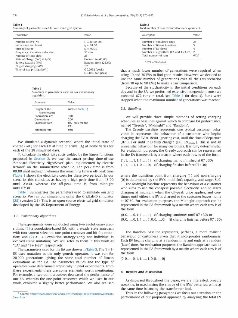
To calculate the electricity costs yielded by the fitness functionsproposed in Section 2, we use the smart pricing time-of-use‘Standard Electricity NightSaver’ plan implemented by electricIreland2 on the summertime schedule. The peak time is from09:00 until midnight, whereas the remaining time is off-peak time(Table 1 shows the electricity costs for these two periods). In ourscenario, this translates as having a high-peak time from 18:00until 23:30, whereas the off-peak time is from midnightuntil 07:30.

Table 1 summarises the parameters used to simulate our gridscenario. We ran our simulations using the GridLab-D simulator[28] (version 2.3). This is an open source electrical grid simulatordeveloped by the US Department of Energy.

3.2. Evolutionary algorithms

The experiments were conducted using two evolutionary algo-rithms: (1) a population-based EA, with a steady state approachwith tournament selection, one-point crossover and bit-flip muta-tion; and (2) a 1þ1-evolution strategy (only one individual isevolved using mutation). We will refer to them in this work as“EA” and “1þ1-ES”, respectively.

The parameters used for the EA are shown in Table 2. The 1þ1-ES uses mutation as the only genetic operator. It was run for20,000 generations, giving the same total number of fitnessevaluations as the EA. The parameter values and the type ofoperators were determined empirically in pilot experiments. Fromthese experiments there are some elements worth mentioning.For example, a two-point crossover decreased the performance ofour EA, whereas the one-point crossover, which we used in ourwork, exhibited a slightly better performance. We also realised

that a much lower number of generations were required whenusing 10 and 30 EVs to find good results. However, we decided touse the same number of generations over all the EVs scenarios(from 10 up to 90 EVs) to make a fair comparison.

Because of the stochasticity in the initial conditions on eachday and in the EA, we performed extensive independent runs (weexecuted 672 runs in total, see Table 3 for details). Runs werestopped when the maximum number of generations was reached.

3.3. Baselines

We will provide three simple methods of setting chargingschedules as baselines against which to compare EA performance,named “Greedy”, “Midnight” and “Random”.

The Greedy baseline represents one typical customer beha-viour. It represents the behaviour of a customer who beginscharging the EV at 18:00, ignoring cost, until the time of departure(07:30) or until it is fully charged (i.e., SoCmaxm ). This is not anunrealistic behaviour for many customers. It is fully deterministic.For evaluation purposes, the Greedy approach can be representedin the EA framework by a matrix where each row is of the form

f1;1;…;1;1;1;…;1g ðif charging has not finished at 07 : 30Þf1;1;…;1;1;0;…;0g ðif charging finishes before 07 : 30Þ

where the transition point from charging (1) and non-charging(0) is determined by the EV's initial SoC, capacity, and target SoC.

The Midnight baseline represents the behaviour of a customerwho aims to use the cheapest possible electricity, and so startscharging at midnight when the off-peak price applies, and con-tinues until either the EV is charged or the customer leaves homeat 07:30. For evaluation purposes, the Midnight approach can berepresented in the EA framework by a matrix where each row is ofthe form

f0;0;…;0;1;1;…;1g ðif charging continues until 07 : 30Þ;orf0;0;…;0;1;1;…;1;0;0;…;0g ðif charging finishes before 07 : 30Þ

The Random baseline represents, perhaps, a more realisticbehaviour of customers given that it incorporates randomness.Each EV begins charging at a random time and ends at a random(later) time. For evaluation purposes, the Random approach can berepresented in the EA framework by a matrix where each row is ofthe form

½0;0;…;0;1;1;…;1;0;0;…;0�

4. Results and discussion

As discussed throughout the paper, we are interested, broadlyspeaking, in maximising the charge of the EVs’ batteries, while atthe same time balancing the transformer load.

Thus, in the following paragraphs we focus our attention on theperformance of our proposed approach by analysing the total EV

Table 1Summary of parameters used for our smart grid system.

Parameter Value

Number of EVs (N) f10;30;60;90gInitial time and latest ti ¼ 18:00,time to charge tf ¼ 07:30Frequency of making a decision 30 minNumber of time slots T 28State of Charge (SoC) at ti (%) Uniform in ½40;60�Battery capacity (kW) Random from f24;60gPlug-in charging (kW) 1.7Time-of-use pricing (kWh) € 0.2062 (peak)

€ 0.1019 (off peak)

Table 2Summary of parameters used for our evolutionaryalgorithm.

Parameter Value

Length of thechromosome

NT (see Table 1)

Population size 100Generations 200Crossover rate 0.5 (only for the

EA)Mutation rate 0.01

Table 3Total number of runs executed for our experiments.

Description Value

Number of simulated days 28Number of fitness functions 3Number of EV fleets 4Number of algorithms (EA and 1þ1-ES) 2Total number of runs 672a

a 672¼ 28n3n4n2.

2 Source: https://www.electricireland.ie/switchchange/detailsValueRewardNightSaver.htm


https://www.electricireland.ie/switchchange/detailsValueRewardNightSaver.htm

https://www.electricireland.ie/switchchange/detailsValueRewardNightSaver.htm

load at the transformer over time and how this translates tocharge in the EVs’ batteries by analysing the initial and final stateof charge. We also analyse what the impact is on the peak-to-average ratio. Finally, we discuss and analyse the implications ofthe proposed approach in terms of electricity costs.

4.1. Overall performance

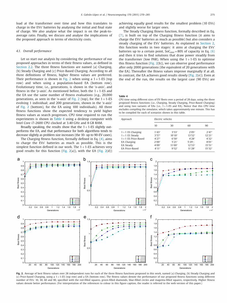
Let us start our analysis by considering the performance of ourproposed approaches in terms of their fitness values, as defined inSection 2.2. The three fitness functions are named (a) Charging,(b) Steady Charging and (c) Price-Based Charging. According to allthree definitions of fitness, higher fitness values are preferred.Their performance is shown in Fig. 2 when using a 1þ1-ES (toprow) and when using a population-based EA (bottom row).Evolutionary time, i.e., generations, is shown in the ‘x-axis’, andfitness in the ‘y-axis’. As mentioned before, both the 1þ1-ES andthe EA use the same number of fitness evaluations (e.g., 20,000generations, as seen in the ‘x-axis’ of Fig. 2 (top), for the 1þ1-ESevolving 1 individual; and 200 generations, shown in the ‘x-axis’of Fig. 2 (bottom), for the EA using 100 individuals). All threefitness functions show the expected tendency to yield higherfitness values as search progresses. CPU time required to run theexperiments is shown in Table 4 using a desktop computer withIntel Core i7-2600 CPU clocked at 3.40 GHz and 8 GB RAM.

Broadly speaking, the results show that the 1þ1-ES slightly out-performs the EA, and that performance for both algorithms tends todecrease slightly as problem size increases (the 10- up to 90-EV cases).

The Charging fitness function, formally defined in Eq. (4), aimsto charge the EVs' batteries as much as possible. This is thesimplest function defined in our work. The 1þ1-ES achieves verygood results for this function (Fig. 2(a)), with the EA (Fig. 2(d))

achieving equally good results for the smallest problem (10 EVs)and slightly worse for larger ones.

The Steady Charging fitness function, formally described in Eq.(7), is built on top of the Charging fitness function (it aims tocharge the EVs’ batteries as much as possible) but also considers asteady charging of the EVs’ batteries. As explained in Section 2,this function works in two stages: it aims at charging the EVs’batteries up to a certain point, SoCmin¼80% of capacity in Eq. (6)and then it tries to find solutions that draw power steadily fromthe transformer (low PAR). When using the 1þ1-ES to optimisethis fitness function (Fig. 2(b)), we can observe good performanceafter only 2000 generations (the equivalent of 20 generations withthe EA). Thereafter the fitness values improve marginally if at all.In contrast, the EA achieves good results slowly (Fig. 2(e)). Even atthe end of the run, the results on the largest case (90 EVs) are

0.2 0.4 0.6 0.8 1 1.2 1.4 1.6 1.8 20

0.1

0.2

0.3

0.4

0.5

0.6

0.7

0.8

0.9

1

Generations

Bes

t fitn

ess

0.2 0.4 0.6 0.8 1 1.2 1.4 1.6 1.8 20

0.5

1

1.5

Generations

Bes

t fitn

ess

0.2 0.4 0.6 0.8 1 1.2 1.4 1.6 1.8 20

0.2

0.4

0.6

0.8

1

1.2

1.4

1.6

1.8

2

Generations

Bes

t fitn

ess

20 40 60 80 100 120 140 160 180 2000

0.1

0.2

0.3

0.4

0.5

0.6

0.7

0.8

0.9

1

Generations

Bes

t fitn

ess

20 40 60 80 100 120 140 160 180 2000

0.5

1

1.5

Generations

Bes

t fitn

ess

20 40 60 80 100 120 140 160 180 2000

0.2

0.4

0.6

0.8

1

1.2

1.4

1.6

1.8

2

Generations

Bes

t fitn

ess

Fig. 2. Average of best fitness values over 28 independent runs for each of the three fitness functions proposed in this work, named (a) Charging, (b) Steady Charging and(c) Price-based Charging, using a 1þ1-ES (top row) and a EA (bottom row). The fitness values denote the performance of our proposed fitness functions using differentnumber of EVs: 10, 30, 60 and 90, specified with the red-filled squares, green-filled diamonds, blue-filled circles and magenta-filled squares, respectively. Higher fitnessvalues denote better performance. (For interpretation of the references to colour in this figure caption, the reader is referred to the web version of this paper.)

Table 4CPU time using different sizes of EV fleets over a period of 28 days, using the threeproposed fitness functions (i.e., Charging, Steady Charging, Price-Based Charging)and using two variants of EAs (i.e., 1þ1-ES and EA). Notice that this CPU timeexcludes compiling the simulator, which takes approximately one minute. This hasto be compiled for each of scenarios shown in this table.

Approach Electric vehicles

10 30 60 90

1þ1 ES Charging 1043″ 3053″ 2005″ 2047″1þ1 ES Steady 3057″ 10010″ 13052″ 12021″1þ1 ES Price-Based 4027″ 6050″ 4028″ 4032″EA Charging 2000″ 5021″ 50290; 8001″EA Steady 4009″ 11000″ 12053″ 15051″EA Price-Based 4011″ 9052″ 11028″ 15032″


improving but are still not quite as good as for the 1þ1-ES. Thismay suggest that longer runs would allow the EA to continue toimprove, eventually out-performing the 1þ1-ES.

The third and last fitness function proposed in our work, namedPrice-Based Charging, formally described in Eq. (9), works in threestages: it aims to charge the EVs' batteries up to a certain point (i.e.,SoC 80%), then it tries to reduce electricity costs given a pricingsignal. Once search is able to meet these two targets, it tries toachieve a constancy at the transformer load (Eq. (6)). The perfor-mance of this function when using the 1þ1-ES is depicted in Fig. 2(c). We can see a trend similar to that of the previous two fitnessfunctions when using this particular algorithm. That is, performancedrops for the larger problems (60- and 90-EV cases). The EA (Fig. 2(f)) marginally out-performs the 1þ1-ES on the 10-EV case, butagain performance is somewhat worse for larger problems.

From the above discussion, we have learned that both algo-rithms are capable of improving all three fitness functions, and

that the 1þ1-ES has a slight advantage over the EA. However thefunctions' impact on the individual goals of the work (transformerload, SoC, PAR, and electricity costs) is not yet clear. This isparticularly so for the functions that work in two phases (i.e.,the Steady- and Price-Based Charging), due to the fact that thefitness values are a combination of these stages. In the followingsections, the fitness functions’ impact on the individual goals willbe examined in turn and compared to the baselines described inSection 3 (i.e., the Greedy, Midnight, and Random baselines).

4.2. Transformer load

Let us consider the load over time, averaged over a period of 28simulated days, depicted in Figs. 3, 4, 5 and 6, for 10, 30, 60 and 90EVs, respectively, when using the Greedy, Midnight and Randombaselines, and using both the 1þ1-ES and a EA with the threefitness functions.

18 19 20 21 22 23 0 1 2 3 4 5 6 70

2

4

6

8

10

12

14

16

18

Timeslots during day (30-minute timeslots)

Ave

rage

tran

sfor

mer

load

(KW

)

18 19 20 21 22 23 0 1 2 3 4 5 6 70

2

4

6

8

10

12

14

16

18


Ave

rage

tran

sfor

mer

load

(KW

)

18 19 20 21 22 23 0 1 2 3 4 5 6 70

2

4

6

8

10

12

14

16

18


Ave

rage

tran

sfor

mer

load

(KW

)

18 19 20 21 22 23 0 1 2 3 4 5 6 70

2

4

6

8

10

12

14

16

18


Ave

rage

tran

sfor

mer

load

(KW

)

18 19 20 21 22 23 0 1 2 3 4 5 6 70

2

4

6

8

10

12

14

16

18


Ave

rage

tran

sfor

mer

load

(KW

)

18 19 20 21 22 23 0 1 2 3 4 5 6 70

2

4

6

8

10

12

14

16

18


Ave

rage

tran

sfor

mer

load

(KW

)

18 19 20 21 22 23 0 1 2 3 4 5 6 70

2

4

6

8

10

12

14

16

18


Ave

rage

tran

sfor

mer

load

(KW

)

18 19 20 21 22 23 0 1 2 3 4 5 6 70

2

4

6

8

10

12

14

16

18


Ave

rage

tran

sfor

mer

load

(KW

)

18 19 20 21 22 23 0 1 2 3 4 5 6 70

2

4

6

8

10

12

14

16

18


Ave

rage

tran

sfor

mer

load

(KW

)

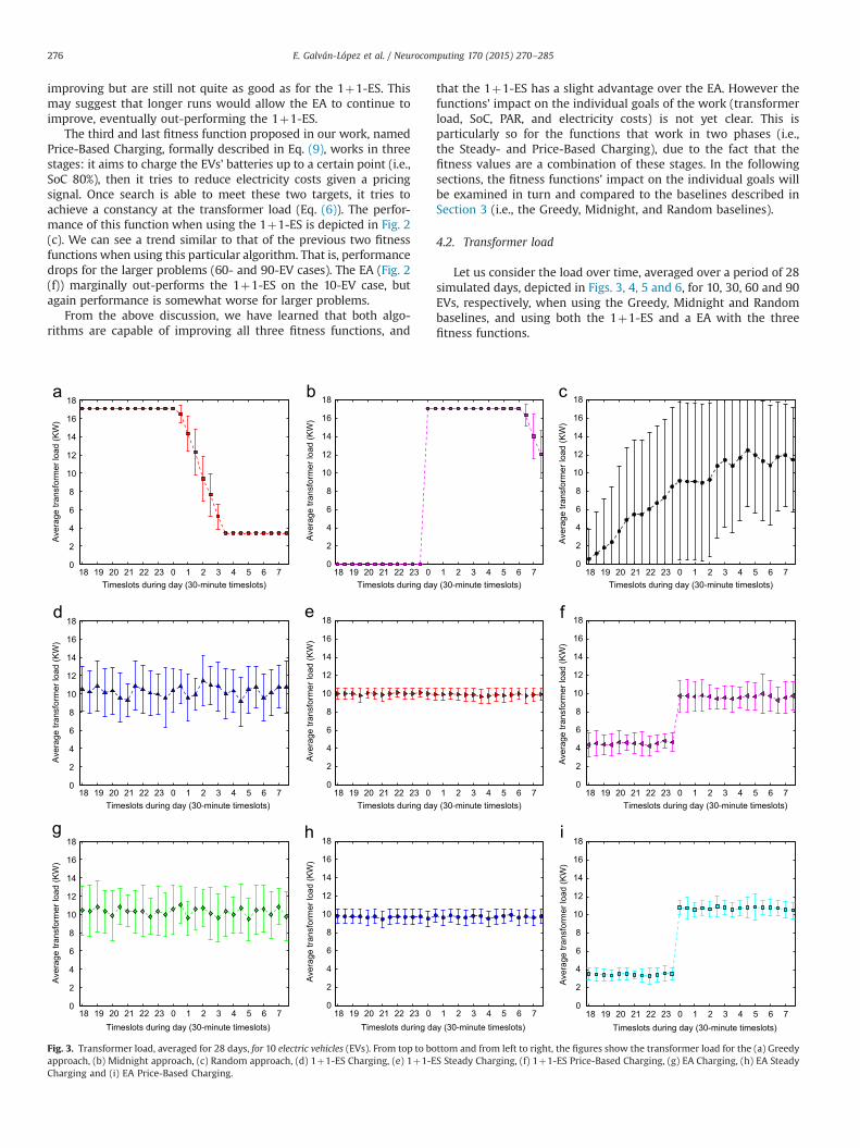
Fig. 3. Transformer load, averaged for 28 days, for 10 electric vehicles (EVs). From top to bottom and from left to right, the figures show the transformer load for the (a) Greedyapproach, (b) Midnight approach, (c) Random approach, (d) 1þ1-ES Charging, (e) 1þ1-ES Steady Charging, (f) 1þ1-ES Price-Based Charging, (g) EA Charging, (h) EA SteadyCharging and (i) EA Price-Based Charging.


Results for the Greedy approach are shown with red squares inFigs. 3(a), 4(a), 5(a) and 6(a) (top-left image in all cases). It resultsin a high transformer load from 18:00. Demand begins to dropfrom 00:00 as some EVs become fully charged. It represents one ofthe two worst-case scenarios for transformer load (the other is theMidnight approach, discussed in the next paragraph) because itsimulates that an EV starts charging as soon as it reaches home. Asexpected, this approach gives a higher transformer load during the18:00–00:00 period than either of the algorithms with any of thethree fitness functions. We can also see that with the Greedyapproach it is not possible to fully charge all the EVs’ batteries foreach of the simulated days since with this method the transformerload never drops to zero, as shown in Figs. 3(a), 4(a), 5(a) and 6(a) for 10, 30, 60 and 90 EVs, respectively. The reason why thishappens is due to three main factors: the battery sizes, the limit oncharging rate, and the period of time during which EVs can becharged (these specifications and their corresponding values areshown in Table 1).

The Midnight approach is depicted with magenta squares inFigs. 3(b), 4(b), 5(b) and 6(b) for 10, 30, 60 and 90 EVs, respectively(top-centre image in all cases). Here, load is zero until 00:00, thenjumps to a maximum and remains at this value until some EVsbecome fully charged. It is equally as bad as the Greedy approach,and in fact, it shows the same transformer load achieved by theGreedy approach, but at a different time. Because of the nature ofthis approach (i.e., starts to charge the EVs at midnight, when theelectricity cost is the lowest) and by considering the previousapproach, which starts charging the EVs 6 h before compared tothis approach, it is clear that none of the EV fleets will be fullycharged at the time of departure, as can be observed in thereferred figures. For instance, if we consider the case with 10EVs, shown in Fig. 3(b) we can see that at 07:30, the averagetransformer load is around 12 kW, whereas for the Greedyapproach, the average transformer load is around 4 kW, depictedin Fig. 3(a). The same trend is observed for the rest of the EV fleets(i.e., 30, 60 and 90 EVs). We will further discuss the implications of

18 19 20 21 22 23 0 1 2 3 4 5 6 70

10

20

30

40

50

60


Ave

rage

tran

sfor

mer

load

(KW

)

18 19 20 21 22 23 0 1 2 3 4 5 6 70

10

20

30

40

50

60


Ave

rage

tran

sfor

mer

load

(KW

)

18 19 20 21 22 23 0 1 2 3 4 5 6 70

10

20

30

40

50

60


Ave

rage

tran

sfor

mer

load

(KW

)

18 19 20 21 22 23 0 1 2 3 4 5 6 70

10

20

30

40

50

60


Ave

rage

tran

sfor

mer

load

(KW

)

18 19 20 21 22 23 0 1 2 3 4 5 6 70

10

20

30

40

50

60


Ave

rage

tran

sfor

mer

load

(KW

)

18 19 20 21 22 23 0 1 2 3 4 5 6 70

10

20

30

40

50

60


Ave

rage

tran

sfor

mer

load

(KW

)

18 19 20 21 22 23 0 1 2 3 4 5 6 70

10

20

30

40

50

60


Ave

rage

tran

sfor

mer

load

(KW

)

18 19 20 21 22 23 0 1 2 3 4 5 6 70

10

20

30

40

50

60


Ave

rage

tran

sfor

mer

load

(KW

)

18 19 20 21 22 23 0 1 2 3 4 5 6 70

10

20

30

40

50

60


Ave

rage

tran

sfor

mer

load

(KW

)

Fig. 4. Transformer load, averaged for 28 days, for 30 electric vehicles (EVs). From top to bottom and from left to right, the figures show the transformer load for the(a) Greedy approach, (b) Midnight approach, (c) Random approach, (d) 1þ1-ES Charging, (e) 1þ1-ES Steady Charging, (f) 1þ1-ES Price-Based Charging, (g) EA Charging,(h) EA Steady Charging and (i) EA Price-Based Charging.


this transformer load when analysing the state of charge, peak toaverage ratio and electricity costs later in this section.

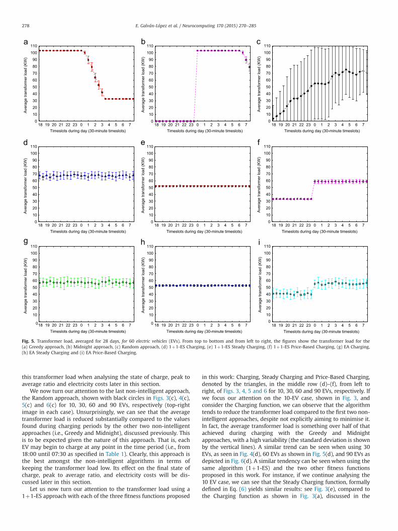
We now turn our attention to the last non-intelligent approach,the Random approach, shown with black circles in Figs. 3(c), 4(c),5(c) and 6(c) for 10, 30, 60 and 90 EVs, respectively (top-rightimage in each case). Unsurprisingly, we can see that the averagetransformer load is reduced substantially compared to the valuesfound during charging periods by the other two non-intelligentapproaches (i.e., Greedy and Midnight), discussed previously. Thisis to be expected given the nature of this approach. That is, eachEV may begin to charge at any point in the time period (i.e., from18:00 until 07:30 as specified in Table 1). Clearly, this approach isthe best amongst the non-intelligent algorithms in terms ofkeeping the transformer load low. Its effect on the final state ofcharge, peak to average ratio, and electricity costs will be dis-cussed later in this section.

Let us now turn our attention to the transformer load using a1þ1-ES approach with each of the three fitness functions proposed

in this work: Charging, Steady Charging and Price-Based Charging,denoted by the triangles, in the middle row (d)–(f), from left toright, of Figs. 3, 4, 5 and 6 for 10, 30, 60 and 90 EVs, respectively. Ifwe focus our attention on the 10-EV case, shown in Fig. 3, andconsider the Charging function, we can observe that the algorithmtends to reduce the transformer load compared to the first two non-intelligent approaches, despite not explicitly aiming to minimise it.In fact, the average transformer load is something over half of thatachieved during charging with the Greedy and Midnightapproaches, with a high variability (the standard deviation is shownby the vertical lines). A similar trend can be seen when using 30EVs, as seen in Fig. 4(d), 60 EVs as shown in Fig. 5(d), and 90 EVs asdepicted in Fig. 6(d). A similar tendency can be seenwhen using thesame algorithm (1þ1-ES) and the two other fitness functionsproposed in this work. For instance, if we continue analysing the10 EV case, we can see that the Steady Charging function, formallydefined in Eq. (6) yields similar results: see Fig. 3(e), compared tothe Charging function as shown in Fig. 3(a), discussed in the

18 19 20 21 22 23 0 1 2 3 4 5 6 70

10

20

30

40

50

60

70

80

90

100

110


Ave

rage

tran

sfor

mer

load

(KW

)

18 19 20 21 22 23 0 1 2 3 4 5 6 70

10

20

30

40

50

60

70

80

90

100

110


Ave

rage

tran

sfor

mer

load

(KW

)

18 19 20 21 22 23 0 1 2 3 4 5 6 70

10

20

30

40

50

60

70

80

90

100

110


Ave

rage

tran

sfor

mer

load

(KW

)

18 19 20 21 22 23 0 1 2 3 4 5 6 70

10

20

30

40

50

60

70

80

90

100

110


Ave

rage

tran

sfor

mer

load

(KW

)

18 19 20 21 22 23 0 1 2 3 4 5 6 70

10

20

30

40

50

60

70

80

90

100

110


Ave

rage

tran

sfor

mer

load

(KW

)

18 19 20 21 22 23 0 1 2 3 4 5 6 70

10

20

30

40

50

60

70

80

90

100

110


Ave

rage

tran

sfor

mer

load

(KW

)

18 19 20 21 22 23 0 1 2 3 4 5 6 70

10

20

30

40

50

60

70

80

90

100

110


Ave

rage

tran

sfor

mer

load

(KW

)

18 19 20 21 22 23 0 1 2 3 4 5 6 70

10

20

30

40

50

60

70

80

90

100

110


Ave

rage

tran

sfor

mer

load

(KW

)

18 19 20 21 22 23 0 1 2 3 4 5 6 70

10

20

30

40

50

60

70

80

90

100

110


Ave

rage

tran

sfor

mer

load

(KW

)



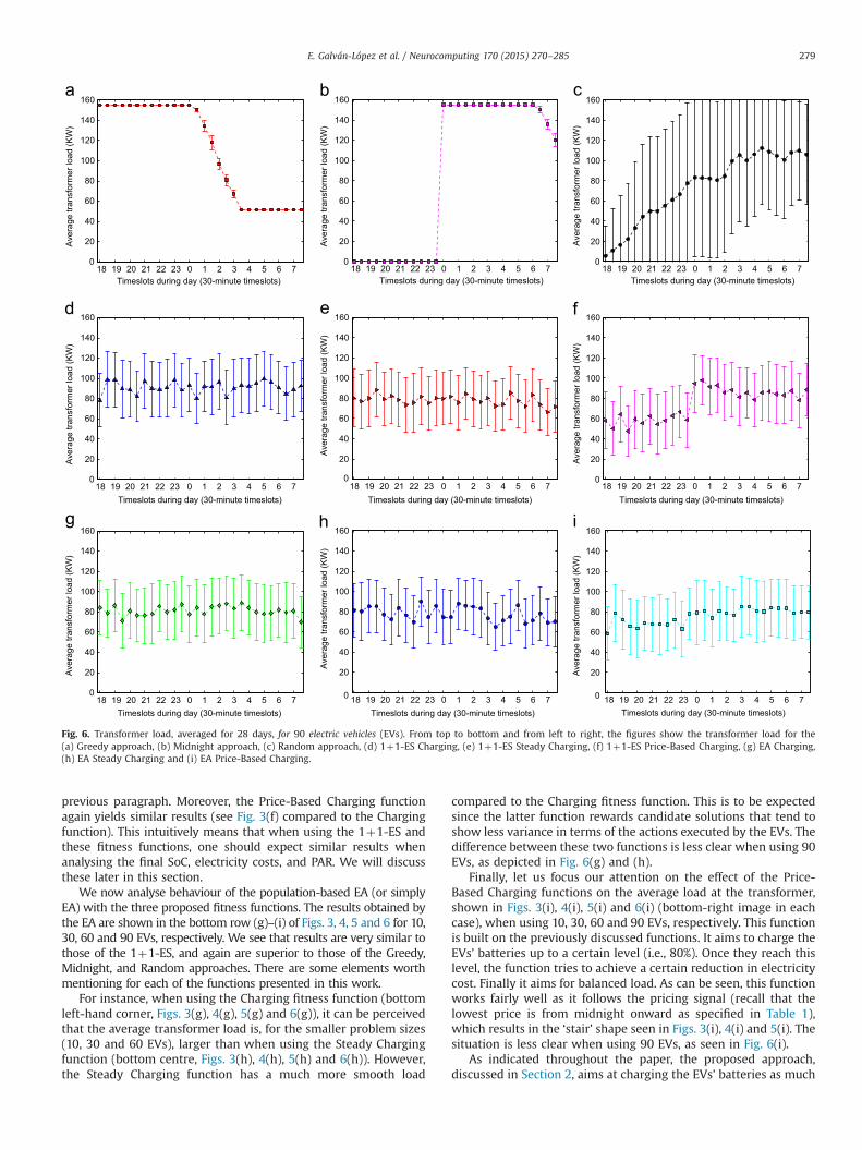
previous paragraph. Moreover, the Price-Based Charging functionagain yields similar results (see Fig. 3(f) compared to the Chargingfunction). This intuitively means that when using the 1þ1-ES andthese fitness functions, one should expect similar results whenanalysing the final SoC, electricity costs, and PAR. We will discussthese later in this section.

We now analyse behaviour of the population-based EA (or simplyEA) with the three proposed fitness functions. The results obtained bythe EA are shown in the bottom row (g)–(i) of Figs. 3, 4, 5 and 6 for 10,30, 60 and 90 EVs, respectively. We see that results are very similar tothose of the 1þ1-ES, and again are superior to those of the Greedy,Midnight, and Random approaches. There are some elements worthmentioning for each of the functions presented in this work.

For instance, when using the Charging fitness function (bottomleft-hand corner, Figs. 3(g), 4(g), 5(g) and 6(g)), it can be perceivedthat the average transformer load is, for the smaller problem sizes(10, 30 and 60 EVs), larger than when using the Steady Chargingfunction (bottom centre, Figs. 3(h), 4(h), 5(h) and 6(h)). However,the Steady Charging function has a much more smooth load

compared to the Charging fitness function. This is to be expectedsince the latter function rewards candidate solutions that tend toshow less variance in terms of the actions executed by the EVs. Thedifference between these two functions is less clear when using 90EVs, as depicted in Fig. 6(g) and (h).

Finally, let us focus our attention on the effect of the Price-Based Charging functions on the average load at the transformer,shown in Figs. 3(i), 4(i), 5(i) and 6(i) (bottom-right image in eachcase), when using 10, 30, 60 and 90 EVs, respectively. This functionis built on the previously discussed functions. It aims to charge theEVs’ batteries up to a certain level (i.e., 80%). Once they reach thislevel, the function tries to achieve a certain reduction in electricitycost. Finally it aims for balanced load. As can be seen, this functionworks fairly well as it follows the pricing signal (recall that thelowest price is from midnight onward as specified in Table 1),which results in the ‘stair’ shape seen in Figs. 3(i), 4(i) and 5(i). Thesituation is less clear when using 90 EVs, as seen in Fig. 6(i).

As indicated throughout the paper, the proposed approach,discussed in Section 2, aims at charging the EVs’ batteries as much

18 19 20 21 22 23 0 1 2 3 4 5 6 70

20

40

60

80

100

120

140

160


Ave

rage

tran

sfor

mer

load

(KW

)

18 19 20 21 22 23 0 1 2 3 4 5 6 70

20

40

60

80

100

120

140

160


Ave

rage

tran

sfor

mer

load

(KW

)

18 19 20 21 22 23 0 1 2 3 4 5 6 70

20

40

60

80

100

120

140

160


Ave

rage

tran

sfor

mer

load

(KW

)

18 19 20 21 22 23 0 1 2 3 4 5 6 70

20

40

60

80

100

120

140

160


Ave

rage

tran

sfor

mer

load

(KW

)

18 19 20 21 22 23 0 1 2 3 4 5 6 70

20

40

60

80

100

120

140

160


Ave

rage

tran

sfor

mer

load

(KW

)

18 19 20 21 22 23 0 1 2 3 4 5 6 70

20

40

60

80

100

120

140

160


Ave

rage

tran

sfor

mer

load

(KW

)

18 19 20 21 22 23 0 1 2 3 4 5 6 70

20

40

60

80

100

120

140

160


Ave

rage

tran

sfor

mer

load

(KW

)

18 19 20 21 22 23 0 1 2 3 4 5 6 70

20

40

60

80

100

120

140

160


Ave

rage

tran

sfor

mer

load

(KW

)

18 19 20 21 22 23 0 1 2 3 4 5 6 70

20

40

60

80

100

120

140

160


Ave

rage

tran

sfor

mer

load

(KW

)



as possible at the time of departure, balancing transformer load,and reducing consumer electricity costs. Only the first of thesegoals is captured in the Charging function defined in Eq. (4),whereas the Steady Charging considers the first two goals, andPrice-Based Charging considers all three.

4.3. State of charge

From our previous analysis on the transformer load and thethree fitness functions, we know that the Charging function willachieve a higher final state of charge (SoC) compared to thatachieved by the two other functions. However, it remains unclearexactly what final SoC will be achieved for both the non-intelligentapproaches (i.e., Greedy, Midnight and Random) and the EAapproaches (i.e., 1þ1-ES and population-based EA) using each ofthe three fitness functions.

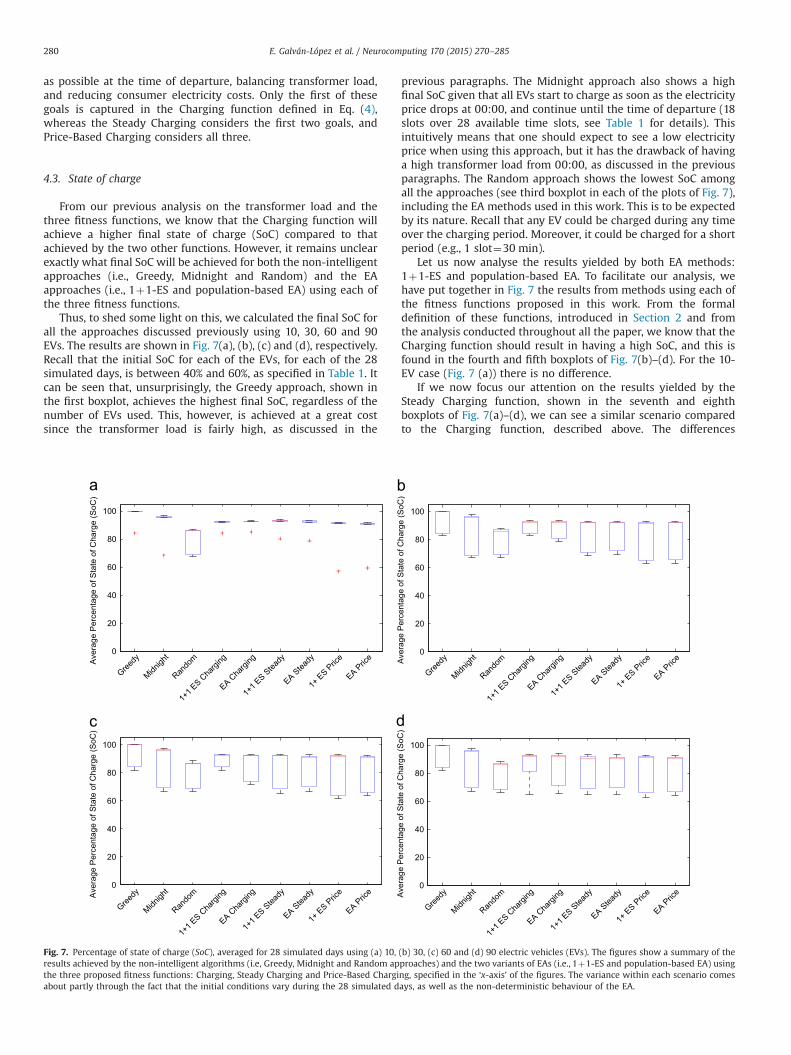
Thus, to shed some light on this, we calculated the final SoC forall the approaches discussed previously using 10, 30, 60 and 90EVs. The results are shown in Fig. 7(a), (b), (c) and (d), respectively.Recall that the initial SoC for each of the EVs, for each of the 28simulated days, is between 40% and 60%, as specified in Table 1. Itcan be seen that, unsurprisingly, the Greedy approach, shown inthe first boxplot, achieves the highest final SoC, regardless of thenumber of EVs used. This, however, is achieved at a great costsince the transformer load is fairly high, as discussed in the

previous paragraphs. The Midnight approach also shows a highfinal SoC given that all EVs start to charge as soon as the electricityprice drops at 00:00, and continue until the time of departure (18slots over 28 available time slots, see Table 1 for details). Thisintuitively means that one should expect to see a low electricityprice when using this approach, but it has the drawback of havinga high transformer load from 00:00, as discussed in the previousparagraphs. The Random approach shows the lowest SoC amongall the approaches (see third boxplot in each of the plots of Fig. 7),including the EA methods used in this work. This is to be expectedby its nature. Recall that any EV could be charged during any timeover the charging period. Moreover, it could be charged for a shortperiod (e.g., 1 slot¼30 min).

Let us now analyse the results yielded by both EA methods:1þ1-ES and population-based EA. To facilitate our analysis, wehave put together in Fig. 7 the results from methods using each ofthe fitness functions proposed in this work. From the formaldefinition of these functions, introduced in Section 2 and fromthe analysis conducted throughout all the paper, we know that theCharging function should result in having a high SoC, and this isfound in the fourth and fifth boxplots of Fig. 7(b)–(d). For the 10-EV case (Fig. 7 (a)) there is no difference.

If we now focus our attention on the results yielded by theSteady Charging function, shown in the seventh and eighthboxplots of Fig. 7(a)–(d), we can see a similar scenario comparedto the Charging function, described above. The differences

0

20

40

60

80

100

Greedy

Midnigh

t

Rando

m

1+1 E

S Cha

rging

EA Cha

rging

1+1 E

S Stea

dy

EA Stea

dy

1+ E

S Pric

e

EA Pric

eAve

rage

Per

cent

age

of S

tate

of C

harg

e (S

oC)

0

20

40

60

80

100

Greedy

Midnigh

t

Rando

m

1+1 E

S Cha

rging

EA Cha

rging

1+1 E

S Stea

dy

EA Stea

dy

1+ E

S Pric

e

EA Pric

eAve

rage

Per

cent

age

of S

tate

of C

harg

e (S

oC)

0

20

40

60

80

100

Greedy

Midnigh

t

Rando

m

1+1 E

S Cha

rging

EA Cha

rging

1+1 E

S Stea

dy

EA Stea

dy

1+ E

S Pric

e

EA Pric

eAve

rage

Per

cent

age

of S

tate

of C

harg

e (S

oC)

0

20

40

60

80

100

Greedy

Midnigh

t

Rando

m

1+1 E

S Cha

rging

EA Cha

rging

1+1 E

S Stea

dy

EA Stea

dy

1+ E

S Pric

e

EA Pric

eAve

rage

Per

cent

age

of S

tate

of C

harg

e (S

oC)

Fig. 7. Percentage of state of charge (SoC), averaged for 28 simulated days using (a) 10, (b) 30, (c) 60 and (d) 90 electric vehicles (EVs). The figures show a summary of theresults achieved by the non-intelligent algorithms (i.e, Greedy, Midnight and Random approaches) and the two variants of EAs (i.e., 1þ1-ES and population-based EA) usingthe three proposed fitness functions: Charging, Steady Charging and Price-Based Charging, specified in the ‘x-axis’ of the figures. The variance within each scenario comesabout partly through the fact that the initial conditions vary during the 28 simulated days, as well as the non-deterministic behaviour of the EA.


between the 1þ1-ES and EA, if any, are small. However, the SoCachieved by this Steady Charging function is often lower than thatof the Charging function. This is also to be expected given thefeatures of the former function. That is, it tends to charge an EV asmuch as possible while at the same trying to make a lowfluctuation at the transformer load. Thus, as a result of the lastconstraint, one should expect a lower SoC.

The final fitness function, Price-Based Charging function,shown in the last two boxplots of Fig. 7(a)–(d), shows a slightlylower SoC compared to the previous fitness functions, regardlessof the EA approach used. Again, by analysing both the fitnessfunction and the results on the transformer load, we can see thatthe rather erratic behaviour observed on the transformer loadshould result on having a lower SoC compared to the other twofunctions, as discussed in the previous paragraphs.

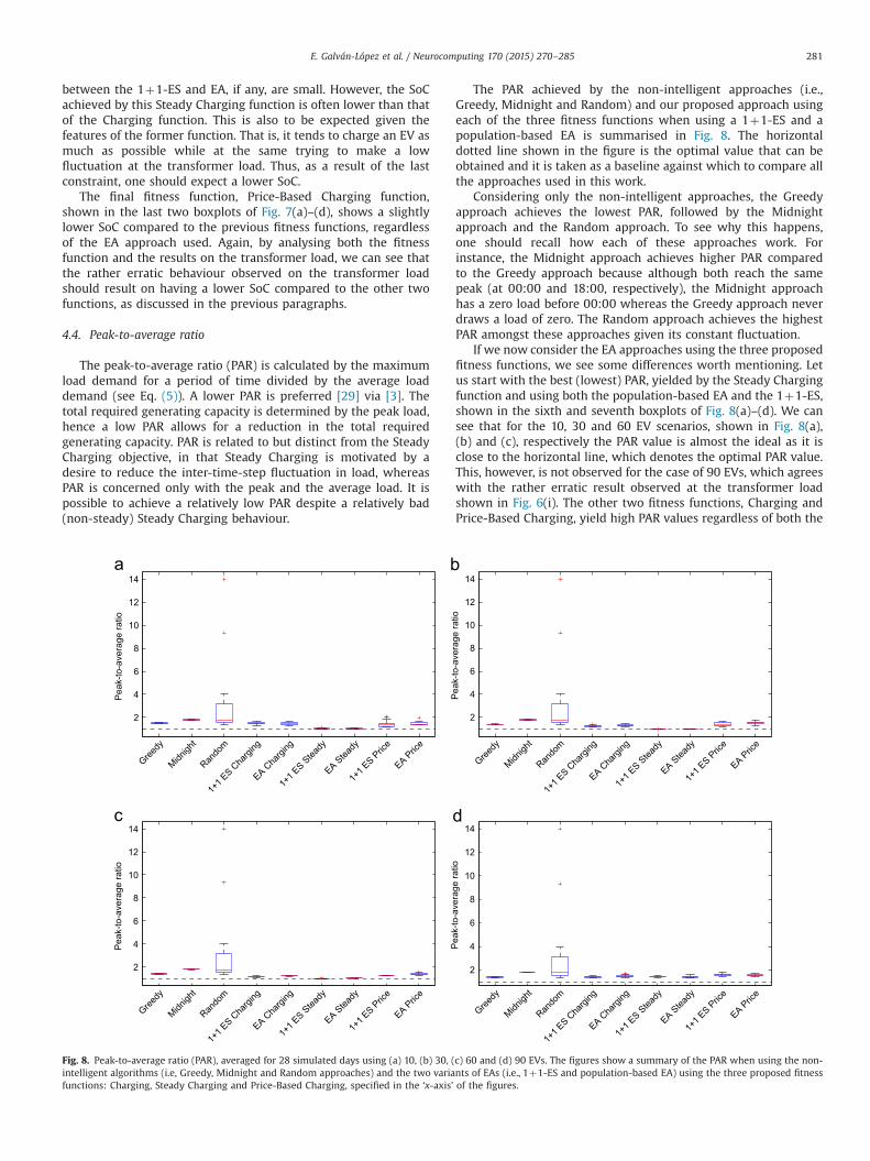
4.4. Peak-to-average ratio

The peak-to-average ratio (PAR) is calculated by the maximumload demand for a period of time divided by the average loaddemand (see Eq. (5)). A lower PAR is preferred [29] via [3]. Thetotal required generating capacity is determined by the peak load,hence a low PAR allows for a reduction in the total requiredgenerating capacity. PAR is related to but distinct from the SteadyCharging objective, in that Steady Charging is motivated by adesire to reduce the inter-time-step fluctuation in load, whereasPAR is concerned only with the peak and the average load. It ispossible to achieve a relatively low PAR despite a relatively bad(non-steady) Steady Charging behaviour.

The PAR achieved by the non-intelligent approaches (i.e.,Greedy, Midnight and Random) and our proposed approach usingeach of the three fitness functions when using a 1þ1-ES and apopulation-based EA is summarised in Fig. 8. The horizontaldotted line shown in the figure is the optimal value that can beobtained and it is taken as a baseline against which to compare allthe approaches used in this work.

Considering only the non-intelligent approaches, the Greedyapproach achieves the lowest PAR, followed by the Midnightapproach and the Random approach. To see why this happens,one should recall how each of these approaches work. Forinstance, the Midnight approach achieves higher PAR comparedto the Greedy approach because although both reach the samepeak (at 00:00 and 18:00, respectively), the Midnight approachhas a zero load before 00:00 whereas the Greedy approach neverdraws a load of zero. The Random approach achieves the highestPAR amongst these approaches given its constant fluctuation.

If we now consider the EA approaches using the three proposedfitness functions, we see some differences worth mentioning. Letus start with the best (lowest) PAR, yielded by the Steady Chargingfunction and using both the population-based EA and the 1þ1-ES,shown in the sixth and seventh boxplots of Fig. 8(a)–(d). We cansee that for the 10, 30 and 60 EV scenarios, shown in Fig. 8(a),(b) and (c), respectively the PAR value is almost the ideal as it isclose to the horizontal line, which denotes the optimal PAR value.This, however, is not observed for the case of 90 EVs, which agreeswith the rather erratic result observed at the transformer loadshown in Fig. 6(i). The other two fitness functions, Charging andPrice-Based Charging, yield high PAR values regardless of both the

2

4

6

8

10

12

14

Greedy

Midnigh

t

Rando

m

1+1 E

S Cha

rging

EA Cha

rging

1+1 E

S Stea

dy

EA Stea

dy

1+1 E

S Pric

e

EA Pric

e

Pea

k-to

-ave

rage

ratio

2

4

6

8

10

12

14

Greedy

Midnigh

t

Rando

m

1+1 E

S Cha

rging

EA Cha

rging

1+1 E

S Stea

dy

EA Stea

dy

1+1 E

S Pric

e

EA Pric

e

Pea

k-to

-ave

rage

ratio

2

4

6

8

10

12

14

Greedy

Midnigh

t

Rando

m

1+1 E

S Cha

rging

EA Cha

rging

1+1 E

S Stea

dy

EA Stea

dy

1+1 E

S Pric

e

EA Pric

e

Pea

k-to

-ave

rage

ratio

2

4

6

8

10

12

14

Greedy

Midnigh

t

Rando

m

1+1 E

S Cha

rging

EA Cha

rging

1+1 E

S Stea

dy

EA Stea

dy

1+1 E

S Pric

e

EA Pric

e

Pea

k-to

-ave

rage

ratio

Fig. 8. Peak-to-average ratio (PAR), averaged for 28 simulated days using (a) 10, (b) 30, (c) 60 and (d) 90 EVs. The figures show a summary of the PAR when using the non-intelligent algorithms (i.e, Greedy, Midnight and Random approaches) and the two variants of EAs (i.e., 1þ1-ES and population-based EA) using the three proposed fitnessfunctions: Charging, Steady Charging and Price-Based Charging, specified in the ‘x-axis’ of the figures.


number of EVs and the type of EA employed. This is in fact to beexpected. For the Charging function, one should recall that thisfunction does not consider to reward candidate solutions based ona low fluctuation of the load. On the other hand, the Price-BasedCharging function does consider the fluctuation. However, thehigh PAR observed by this function is mainly caused by the drasticchange in price, resulting in having a fairly big jump in transfor-mer load at 00:00, as observed by the ‘stair’ shape in Figs. 3(i), 4(i),5(i), for 10, 30 and 60 EVs, respectively.

4.5. Electricity costs

As measures of the performance of the plans produced, wehave considered transformer load over time (Figs. 3–6), the state ofcharge (Fig. 7), and the peak-to-average ratio (Fig. 8). It remains toconsider the electricity cost. The natural way to measure this is asthe total cost of the electricity drawn by all EVs over the 28simulated days. However, it is necessary to account for the factthat some plans draw more electricity than others: this is reflectedin the fact that the SoC at the end of the charging period is notuniform. Therefore, we have implemented a measure of electricitycost we will refer to as Equalised Cost. It uses the minimum SoCachieved for each EV as a reference point. Since all EVs achieve thisSoC or higher, the cost up to this SoC can be compared fairly.Therefore, we simply calculate the cost of electricity per EV up tothis minimum SoC, and disregard the electricity drawn after thisSoC. That is, within this metric all EVs are seen as drawing thesame amount of electricity. Furthermore, we calculate the

electricity costs by considering the ToU and the peak and off-peak times, as discussed in Section 3 (a summary is provided inTable 1).

The results of this analysis are shown in Fig. 9, with moredetails shown in Table 5. For all scenarios (10, 30, 60, and 90 EVs)there is quite a clear trend of decrease in Equalised Cost as wemove from the Greedy approach, through the Charging and SteadyCharging to the Price-Based Charging fitness function. The priceper EV for the Greedy approach is relatively constant, at aboutEUR2.18–EUR2.27 per charging period. This relatively high pricereflects the fact that the Greedy approach carries out its chargingas early as possible, as seen in Figs. 3–6, coinciding with the peakcharging period. Obviously, the Midnight approach results in thelowest Equalised Cost given that it only uses the cheapestelectricity cost. The Random approach also yields some fairly lowEqualised Costs, although with a high variance. The reason thelatter approach yields some low Equalised Costs is due to the factthat the off-peak period is longer than the peak period (see Table 1for details).

The Charging and Steady Charging fitness functions tend tospread the load out more, hence as a by-product tend to takebetter advantage of the off-peak charging period, again as seen inFigs. 3–6. The two are comparable, though Steady Chargingspreads the load out slightly more and achieves slightly loweroverall price.

However, the Price-Based Charging fitness function explicitlyrewards low prices, and so is capable of achieving lower prices:approximately EUR1.40 for 10 EVs, up to EUR1.67 for 90 EVs, when

0.5

1

1.5

2

Greedy

Midnigh

t

Rando

m

1+1 E

S Cha

rging

EA Cha

rging

1+1 E

S Stea

dy

EA Stea

dy

1+1 E

S Pric

e

EA Pric

e

Mea

n E

qual

ised

Cos

t (E

uros

)

0.5

1

1.5

2

Greedy

Midnigh

t

Rando

m

1+1 E

S Cha

rging

EA Cha

rging

1+1 E

S Stea

dy

EA Stea

dy

1+1 E

S Pric

e

EA Pric

e

Mea

n E

qual

ised

Cos

t (E

uros

)

0.5

1

1.5

2

Greedy

Midnigh

t

Rando

m

1+1 E

S Cha

rging

EA Cha

rging

1+1 E

S Stea

dy

EA Stea

dy

1+1 E

S Pric

e

EA Pric

e

Mea

n E

qual

ised

Cos

t (E

uros

)

0.5

1

1.5

2

Greedy

Midnigh

t

Rando

m

1+1 E

S Cha

rging

EA Cha

rging

1+1 E

S Stea

dy

EA Stea

dy

1+1 E

S Pric

e

EA Pric

e

Mea

n E

qual

ised

Cos

t (E

uros

)

Fig. 9. Electricity costs, in euros, averaged for the number of electric vehicles used (a) 10, (b) 30, (c) 60 and (d) 90 electric vehicles. The figures show an average of theelectricity cost when using the non-intelligent algorithms (i.e, Greedy, Midnight and Random approaches) and the two variants of EAs (i.e., 1þ1-ES and population-based EA)using the three proposed fitness functions: Charging, Steady Charging and Price-Based Charging, specified in the ‘x-axis’ of the figures.


using the population-based EA approach. However, its advantageover the other fitness functions, which is very clear for 10, 30 or 60EVs, is far less clear for 90 EVs.

5. Conclusions and future work

We have implemented two variants of evolutionary algorithms(EAs): a 1þ1-ES and a population-based EA to search for efficientcharging schedules for fleets of EVs, achieving good results interms of reducing peak demand and reducing consumers' elec-tricity costs, while maintaining a high overall state of charge ofEVs' batteries. We have tested these approaches on small tomedium fleet sizes – 10, 30, 60 and 90 EVs – using realistic datagenerated by a state of the art grid simulator, over the course of 28simulated days.

We have found that the 1þ1-ES is capable of slightly out-performing a population-based EA, referred to in this work as EA.We have also shown that both the EA and the 1þ1-ES approachexhibit better performance compared against the non-intelligentmethods (i.e., Greedy, Midnight and Random approaches) used inthis work. This is a significant result because each of these non-intelligent methods reflects likely default behaviour for mostconsumers: in the Greedy approach, the EV is simply plugged inand charged up fully as soon as it arrives home each evening; in

the Midnight approach, the EV is plugged in at midnight to takeadvantage of the cheapest electricity cost; and in the Randomapproach, the EV could be charged at any time during thesimulated period for any length of time. In contrast, either of theEAs used in this work produces plans which take advantage oflower-cost pricing in the middle of the night, and at the same timereduce peak demand.

Although numbers of EVs are projected to be in the thousandsor millions, Demand Aggregators may have much smaller fleetsizes. Therefore, the smaller fleet sizes considered here representan important real-world case. The slight disimprovement in theEA's results noted in Section 4 for the 90-EV case is not a cause forgreat concern. However, in future work we hope to scale ourresults up further.

It is an assumption of this work that customers are willing tosubmit their charging schedules to a central authority, e.g., aDemand Aggregator. The intelligent algorithms used in thiswork (i.e., 1þ1-ES and EA) require centralised knowledge (thenumber of EVs and their initial SoC) and centralised control(specification of when each EV should charge, up to 30-mingranularity). This assumption is not unrealistic. As we have seen,customers will do better through centralised control thanthrough the most likely individualised behaviour, the Greedyapproach. However, more informed and more price-consciouscustomers will be willing to deviate from the Greedy approach

Table 5The Equalised Cost is calculated based on the number of kilowatt-hours drawn during peak and off-peak hours, equalized between schedules by taking into account onlyelectricity up to a minimum SoC. The Equalised Cost per EV is calculated based on the Equalised Cost and the number of EVs.

Approach Consumption in kWh during peak hours Consumption in kWh during off-peak hours Equalised Cost Equalised Cost per EV

10 Electric vehiclesGreedy 102.21 7.92 21.88 2.18Midnight 0 110.13 11.22 1.12Random 38.73 71.40 14.32 1.431þ1-ES Charging 60.87 49.26 17.20 1.72EA Charging 65.99 44.14 18.10 1.811þ1-ES Steady Charging 60.05 50.08 17.12 1.71EA Steady Charging 60.96 49.17 17.58 1.751þ1-ES Price-Based Charging 27.35 82.78 13.34 1.33EA Price-Based Charging 27.14 82.99 14.05 1.4030 Electric vehiclesGreedy 307.77 37.06 67.24 2.24Midnight 0 344.84 35.13 1.17Random 81.52 263.31 36.95 1.231þ1-ES Charging 203.80 141.03 56.39 1.87EA Charging 193.34 151.50 55.30 1.841þ1-ES Steady Charging 163.43 181.41 52.18 1.73EA Steady Charging 166.72 178.11 52.52 1.751þ1-ES Price-Based Charging 96.78 248.05 44.88 1.49EA Price-Based Charging 107.40 237.44 46.34 1.5460 Electric vehiclesGreedy 617.41 75.38 134.99 2.24Midnight 0 692.8 70.59 1.17Random 163.54 529.26 73.91 1.231þ1-ES Charging 405.05 287.75 112.79 1.87EA Charging 342.31 350.48 106.30 1.771þ1-ES Steady Charging 313.08 379.72 103.20 1.72EA Steady Charging 319.23 373.56 103.89 1.731þ1-ES Price-Based Charging 200.29 492.51 89.31 1.48EA Price-Based Charging 244.61 448.18 96.10 1.6090 Electric vehiclesGreedy 930.59 128.45 204.97 2.27Midnight 0 1059.05 107.91 1.20Random 246.49 812.56 112.90 1.251þ1-ES Charging 544.94 514.11 163.93 1.82EA Charging 490.65 568.39 159.09 1.761þ1-ES Steady Charging 475.54 583.51 156.34 1.73EA Steady Charging 481.31 577.73 158.11 1.751þ1-ES Price-Based Charging 348.26 710.79 142.25 1.58EA Price-Based Charging 414.73 644.31 151.17 1.67


in order to avail of lower cost periods in the middle of thenight. Such behaviour would lead to decreases in performance,in particular increases in peak demand. Therefore, to apply ourwork customers would have to be either contracted to submitcontrol of charging schedules to the central authority, orinduced to do so via a monetary reward. (Any such monetaryreward is not considered in our calculations of electricitycosts.)

In future work, this assumption could be removed, by model-ling consumers as independently evolving agents seeking toreduce their own costs and maximise their own SoC. The pricesignal would then have to be modulated to induce a steadycharging behaviour. Both the consumer's behaviours and the pricesignal policy could then be optimised in a coevolutionary setup.

We hope that the results achieved by our EA approach usingthe fitness functions proposed in this work and by using a well-developed grid simulator could attract the attention of companiesto adapt this form of machine learning technique.

Acknowledgement

Edgar Galván López's research is funded by an ELEVATE Fellow-ship, the Irish Research Council's Career Development Fellowshipco-funded by Marie Curie Actions. The first author would also liketo thank the TAO group at INRIA Saclay & LRI - Univ. Paris-Sud andCNRS, Orsay, France for hosting him during the outgoing phase ofthe ELEVATE Fellowship. Paula Carroll is funded by a ScienceFoundation Ireland Sustainable Electrical Energy Systems (SEES)Strategic Research Cluster Award. The authors would like to thankall the reviewers for their useful comments that helped us tosignificantly improve our work.

References

[1] COM, Energy 2020—A Strategy for Competitive, Sustainable And SecureEnergy, Technical Report 639, European Union, ⟨http://ec.europa.eu/energy/publications/doc/2011_energy2020_en.pdf⟩, 2010.

[2] Y. Tang, H. He, Z. Ni, J. Wen, X. Sui, Reactive power control of grid-connectedwind farm based on adaptive dynamic programming, Neurocomputing 125(2014) 125–133, Advances in Neural Network Research and ApplicationsSelected Papers from the 9th International Symposium of Neural Networks,July 2012 Advances in Bio-Inspired Computing: Techniques and Applicationshttp://dx.doi.org/http://dx.doi.org/10.1016/j.neucom.2012.07.046 ⟨http://www.sciencedirect.com/science/article/pii/S0925231213001628⟩.

[3] A. Mohsenian-Rad, V. Wong, J. Jatskevich, R. Schober, A. Leon-Garcia, Auton-omous demand-side management based on game-theoretic energy consump-tion scheduling for the future smart grid, IEEE Trans. Smart Grid 1 (3) (2010)320–331. http://dx.doi.org/10.1109/TSG.2010.2089069.

[4] E. Galván-López, C. Harris, L. Trujillo, K.R. Vázquez, S. Clarke, V. Cahill,Autonomous demand-side management system based on Monte Carlo treesearch, in: IEEE International Energy Conference (EnergyCon), IEEE Press,Dubrovnik, Croatia, 2014, pp. 1325–1332.

[5] E. Galván-López, A. Taylor, S. Clarke, V. Cahill, Design of an automatic demand-side management system based on evolutionary algorithms, in: Proceedings ofthe 29th Annual Symposium on Applied Computing, SAC '14, ACM, Gyeongju,Korea, 2014, pp. 525–530.

[6] E. Galvan, C. Harris, I. Dusparic, S. Clarke, V. Cahill, Reducing electricity costs ina dynamic pricing environment, in: Proceedings of the Third IEEE Interna-tional Conference on Smart Grid Communications (SmartGridComm), IEEEPress, Tainan, Taiwan, 2012, pp. 169–174.

[7] A. Collin, J. Acosta, I. Hernando-Gil, S. Djokic, An 11 kV steady state residentialaggregate load model. Part 2: microgeneration and demand-side manage-ment, in: 2011 IEEE Trondheim PowerTech, 2011, pp. 1–8. http://dx.doi.org/10.1109/PTC.2011.6019384.

[8] C. Gellings, The concept of demand-side management for electric utilities,Proc. IEEE 73 (10) (1985) 1468–1470. http://dx.doi.org/10.1109/PROC.1985.13318.

[9] G.M. Masters, Renewable and Efficient Electric Power Systems, Wiley-Inter-science, New York, 2004.

[10] P. Palensky, D. Dietrich, Demand side management: demand response,intelligent energy systems, and smart loads, IEEE Trans. Ind. Informatics 7(August (3)) 381–388. http://dx.doi.org/10.1109/TII.2011.2158841.

[11] G. Strbac, Demand side management: benefits and challenges, Energy Policy36 (12) (2008) 4419–4426. http://dx.doi.org/10.1016/j.enpol.2008.09.030,

Foresight Sustainable Energy Management and the Built Environment Project.doi:http://dx.doi.org/10.1016/j.enpol.2008.09.030, URL ⟨http://www.sciencedirect.com/science/article/pii/S0301421508004606⟩.

[12] Pacific Northwest GridWise Testbed Demonstration Projects, Part I. OlympicPeninsula Project, October 2007.

[13] R. Poli, Analysis of the publications on the applications of particle swarmoptimisation, J. Artif. Evol. Appl. 2008 (2008) 4:1-4:10. http://dx.doi.org/10.1155/2008/685175.

[14] S.D. Ramchurn, P. Vytelingum, A. Rogers, N. Jennings, Agent-based control fordecentralised demand side management in the smart grid, in: The 10thInternational Conference on Autonomous Agents and Multiagent Systems—Volume 1, AAMAS ’11, International Foundation for Autonomous Agents andMultiagent Systems, Richland, SC, 2011, pp. 5–12. ⟨http://dl.acm.org/citation.cfm?id=2030470.2030472⟩.

[15] A.E. Eiben, J.E. Smith, Introduction to Evolutionary Computing, Springer,Berlin, Heidelberg, 2003.

[16] T. Bäck, D.B. Fogel, Z. Michalewicz (Eds.), Evolutionary Computation 1: BasicAlgorithms and Operators, IOP Publishing Ltd., Bristol, UK, 1999.

[17] J. Lohn, G. Hornby, D. Linden, An evolved antenna for deployment on NASA'sSpace Technology 5 mission, in: U.-M. O'Reilly, T. Yu, R. Riolo, B. Worzel (Eds.),Genetic Programming Theory and Practice II, Genetic Programming, vol. 8,Springer, USA, 2005, pp. 301–315.

[18] E. Galván-López, J.M. Swafford, M. O'Neill, A. Brabazon, Evolving a Ms. PacMancontroller using grammatical evolution, in: C.D. Chio, S. Cagnoni, C. Cotta, M.Ebner, A. Ekárt, A. Esparcia-Alcázar, C.K. Goh, J.J.M. Guervós, F. Neri, M. Preuss,J. Togelius, G.N. Yannakakis (Eds.), EvoApplications (1), Lecture Notes inComputer Science, vol. 6024, Springer, Istanbul, Turkey, 2010, pp. 161–170.

[19] E. Galván-López, D. Fagan, E. Murphy, J. Swafford, A. Agapitos, M. O'Neill, A.Brabazon, Comparing the performance of the evolvable π grammaticalevolution genotype-phenotype map to grammatical evolution in the dynamicms. pac-man environment, in: 2010 IEEE Congress on Evolutionary Computa-tion (CEC), 2010, pp. 1–8. http://dx.doi.org/10.1109/CEC.2010.5586508.

[20] E. Galván-López, R. Poli, C. Coello,Reusing code in genetic programming, in: M.Keijzer, U.-M. OReilly, S. Lucas, E. Costa, T. Soule (Eds.), Genetic Programming,Lecture Notes in Computer Science, vol. 3003, Springer, Berlin, Heidelberg,2004, pp. 359–368. http://dx.doi.org/10.1007/978-3-540-24650-3_34.

[21] E. Galvan-Lopez, Efficient graph-based genetic programming representationwith multiple outputs, Int. J. Autom. Comput. 5 (1) (2008) 81–89. http://dx.doi.org/10.1007/s11633-008-0081-4.

[22] J.R. Koza, Human-competitive results produced by genetic programming,Genet. Program. Evolvable Mach. 11 (3–4) (2010) 251–284. http://dx.doi.org/10.1007/s10710-010-9112-3.

[23] J.A.P. Lopes, F.J. Soares, P.M. Almeida, M. Moreira da Silva, Smart chargingstrategies for electric vehicles: enhancing grid performance and maximizingthe use of variable renewable energy resources, in: Proceedings of the 24thInternational Electric Vehicle Symposium and Exposition (EVS24), WorldElectric Vehicle Association (WEVA), World Electric Vehicle Association(WEVA), 2009, pp. 1–11.

[24] J. Soares, B. Canizes, C. Lobo, Z. Vale, H. Morais, Electric vehicle scenariosimulator tool for smart grid operators, Energies 5 (6) (2012) 1881–1899.http://dx.doi.org/10.3390/en5061881. ⟨http://www.mdpi.com/1996-1073/5/6/1881⟩.

[25] P. Wang, J. Huang, Y. Ding, P. Loh, L. Goel, Demand side load management ofsmart grids using intelligent trading/metering/ billing system, in: 2010 IEEEPower and Energy Society General Meeting, 2010, pp. 1–6. http://dx.doi.org/10.1109/PES.2010.5588163.

[26] S.J. Gerssen-Gondelach, A.P. Faaij, Performance of batteries for electric vehicleson short and longer term, J. Power Sources 212 (2012) 111–129.

[27] M. Parvania, M. Fotuhi-Firuzabad, M. Shahidehpour, Optimal demandresponse aggregation in wholesale electricity markets, IEEE Trans. Smart Grid4 (4) (2013) 1957–1965.

[28] D. Chassin, K. Schneider, C. Gerkensmeyer, Gridlab-d: an open-source powersystems modeling and simulation environment, in: IEEE/PES Transmissionand Distribution Conference and Exposition, 2008, pp. 1–5. http://dx.doi.org/10.1109/TDC.2008.4517260.

[29] A.J. Wood, B.F. Wollenberg, Power Generation, Operation, and Control, 2ndedition, Wiley, New York. ⟨http://www.amazon.com/exec/obidos/redirect?tag=citeulike07-20&path=ASIN/0471586994⟩.

Edgar Galván-López received the B.Sc. degree in Infor-matics and Statistics and the M.Sc. degree in ArtificialIntelligence from the Universidad Veracruzana, México,and the Ph.D. degree in Computer Science from theUniversity of Essex, UK, in 1995, 1999 and 2009,respectively. He is currently an IRC/Marie Curie Fellow,in the School of Computer Science and Statistics inTrinity College Dublin, Ireland and INRIA, France. Hehas published over 50 scientific publications. His majorresearch interests are evolutionary algorithms andMonte Carlo tree search. He was the co-organiser ofthe Special Session in “Energy Problems and Evolu-tionary Computation” at the IEEE Congress on Evolu-

tionary Computation 2013 and also the co-chair of the Special Session in GeneticProgramming at the Springer Evolve 2012–2014.


http://ec.europa.eu/energy/publications/doc/2011_energy2020_en.pdf

http://ec.europa.eu/energy/publications/doc/2011_energy2020_en.pdf

dx.doi.org/10.1016/j.neucom.2012.07.046

http://www.sciencedirect.com/science/article/pii/S0925231213001628


http://dx.doi.org/10.1109/TSG.2010.2089069



dx.doi.org/10.1109/PTC.2011.6019384

dx.doi.org/10.1109/PTC.2011.6019384

dx.doi.org/10.1109/PROC.1985.13318

dx.doi.org/10.1109/PROC.1985.13318

http://refhub.elsevier.com/S0925-2312(15)00930-3/sbref9


dx.doi.org/10.1109/TII.2011.2158841

http://dx.doi.org/10.1016/j.enpol.2008.09.030






dx.doi.org/10.1155/2008/685175

dx.doi.org/10.1155/2008/685175

http://dl.acm.org/citation.cfm?id=2030470.2030472

http://dl.acm.org/citation.cfm?id=2030470.2030472

dx.doi.org/10.1109/CEC.2010.5586508

dx.doi.org/10.1007/978-3-540-24650-3_34

http://dx.doi.org/10.1007/s11633-008-0081-4

http://dx.doi.org/10.1007/s11633-008-0081-4

http://dx.doi.org/10.1007/s11633-008-0081-4

http://dx.doi.org/10.1007/s11633-008-0081-4

http://dx.doi.org/10.1007/s10710-010-9112-3

http://dx.doi.org/10.1007/s10710-010-9112-3

http://dx.doi.org/10.1007/s10710-010-9112-3

http://dx.doi.org/10.1007/s10710-010-9112-3

dx.doi.org/10.3390/en5061881

http://www.mdpi.com/1996-1073/5/6/1881

http://www.mdpi.com/1996-1073/5/6/1881

dx.doi.org/10.1109/PES.2010.5588163

dx.doi.org/10.1109/PES.2010.5588163






dx.doi.org/10.1109/TDC.2008.4517260

dx.doi.org/10.1109/TDC.2008.4517260

http://www.amazon.com/exec/obidos/redirect?tag=citeulike07-20&path=ASIN/0471586994



Tom Curran received a B.A.(Mod.), Honours, in ComputerScience (2013) and the M.Sc. in Networks and DistributedSystems (2014) from the School of Computer Science andStatistics at Trinity College Dublin. His current researchinterests include evolutionary algorithms, genetic algo-rithms, genetic programming, energy-based problemsand Monte Carlo-based techniques.

James McDermott is a Lecturer in Business Analytics inUniversity College Dublin, Ireland, and a member of theUniversity College Dublin Centre for Business Analyticsand Complex and Adaptive Systems Lab. His researchinterests are in evolutionary computation for programsynthesis, for music, graphics and design, and foranalytics. He holds a B.Sc. in computer science andmathematics from NUI Galway, Ireland (2000) and aPh.D. in evolutionary computation and computer musicfrom the University of Limerick, Ireland (2008). Hispost-doctoral research was in evolutionary computa-tion, evolutionary design, and genetic programming, inUniversity College Dublin and Massachusetts Institute

of Technology, as an IRCSET/Marie Curie Fellow. He was the co-chair of EvoMUSART2013 and 2014 and publication chair of EuroGP 2015.

Paula Carroll is a Lecturer in Business Analytics inUniversity College Dublin, Ireland, and a member of theUCD Centre for Business Analytics and the UCD Elec-tricity Research Centre. Her research interests are inOperations Research, particularly optimisation techni-ques, focusing on applications of Integer Programmingto network optimisation problems. She holds a B.Sc.from Trinity College Dublin (1986) and an MMangtSc(2005) and Ph.D. (2012) from UCD.


design of an autonomous intelligent demand-side management

Documents