Worcester Polytechnic InstituteDigital WPI

Major Qualifying Projects (All Years) Major Qualifying Projects

October 2009

Design of a Supersonic Wind TunnelPeter James MooreWorcester Polytechnic Institute

Follow this and additional works at: https://digitalcommons.wpi.edu/mqp-all

This Unrestricted is brought to you for free and open access by the Major Qualifying Projects at Digital WPI. It has been accepted for inclusion inMajor Qualifying Projects (All Years) by an authorized administrator of Digital WPI. For more information, please contact digitalwpi@wpi.edu.

Repository CitationMoore, P. J. (2009). Design of a Supersonic Wind Tunnel. Retrieved from https://digitalcommons.wpi.edu/mqp-all/2267

Project: ME-JB3-SWT1

Design of a Supersonic Wind Tunnel

A Major Qualifying Project

Submitted to the Faculty

Of

WORCESTER POLYTECHNIC INSTITUTE

in partial fulfillment of the requirements for the

Degree of Bachelor of Science

in Aerospace Engineering

by

Peter Moore

Date: 28 October 2009

Approved: Prof. John Blandino, MQP Advisor

2

Table of Contents

Abstract ......................................................................................................................................................... 4

Nomenclature ............................................................................................................................................... 5

1. Introduction .............................................................................................................................................. 6

2. Background ............................................................................................................................................... 8

2.1 Historical Note .................................................................................................................................... 8

2.2 Current state of the art ..................................................................................................................... 12

3. Summary of the Method of Characteristics ............................................................................................ 18

4. Wind Tunnel Design, Fabrication, and Assembly .................................................................................... 25

4.1 Vacuum chamber and pump constraints .......................................................................................... 25

4.2 Solid Modeling .................................................................................................................................. 26

4.3 Mechanical Design ............................................................................................................................ 32

4.3.1 Rectangular entry flange ............................................................................................................ 32

4.3.2 Nozzle and test-section assembly .............................................................................................. 34

4.3.3 End Piece and Control Ball Valve ............................................................................................... 39

4.4 Material ............................................................................................................................................. 42

4.5 Construction ...................................................................................................................................... 43

5. Conclusions ............................................................................................................................................. 45

6. Appendix ................................................................................................................................................. 48

6.1 Test Duration: Derivation of Equation (6) ......................................................................................... 48

6.2 MATLAB Codes .................................................................................................................................. 51

6.2.1 Mass flow rate as a function of throat area ............................................................................... 51

6.2.2 Test Duration vs. Mass Flow Rate .............................................................................................. 52

6.2.3 Area-Mach number relation ...................................................................................................... 53

6.2.4 Test Duration vs. Throat Height ................................................................................................. 53

6.3 Method of Characteristics Spreadsheets .......................................................................................... 54

6.3.1 Key Assumptions and Parameters ............................................................................................. 54

6.3.2 Familiarization ............................................................................................................................ 54

6.3.3 Wind tunnel diverging and straightening contour analysis ....................................................... 57

6.4 Designs .............................................................................................................................................. 61

6.5 Slides from Design Presentation on 9 September 2009 ................................................................... 65

3

7. References .............................................................................................................................................. 71

Figure 1. The Langley 11-Inch High Speed Tunnel [4]. © NASA. All Rights Reserved. .................................. 9

Figure 2. Diagram of the Langley 11-Inch HST [3]. © NASA. All Rights Reserved. ........................................ 9

Figure 3. General configuration of an indraft-type supersonic wind tunnel. ............................................. 12

Figure 4. General configuration of a blowdown-type supersonic wind tunnel [17] © Wikimedia

Commons. All Rights Reserved ................................................................................................................... 13

Figure 5. Shockwave system in a supersonic diffuser [15]. © Lehrstuhl fur Thermodynamik. All Rights

Reserved. .................................................................................................................................................... 15

Figure 6. Characteristic lines downstream of a supersonic throat ............................................................. 19

Figure 7. Expansion fan caused by supersonic airflow around a corner .................................................... 19

Figure 8. Geometry of characteristics at a point and impinging characteristics ........................................ 20

Figure 9. The WPI Vacuum Test Facility (VTF) ............................................................................................. 25

Figure 10. Mass flow rate vs. throat area. Created in MATLAB, using Equation 4. .................................... 27

Figure 11. Test duration vs. mass flow rate. Assumes isentropic conditions, initial vacuum chamber

pressure Pi = 6.6875 Pa, and end of run chamber pressure Pe = 53499.6 Pa ............................................. 28

Figure 12. Area-Mach relation for a choked supersonic nozzle. Created in MATLAB. ............................... 30

Figure 13. Test duration vs. throat height. Created in MATLAB. ................................................................ 31

Figure 14: exploded view of tunnel assembly ............................................................................................ 32

Figure 15: rectangular entry flange ............................................................................................................ 32

Figure 16. Image of finished rectangular entry flange. ............................................................................... 33

Figure 17: window flange ............................................................................................................................ 33

Figure 18. Tunnel contour ........................................................................................................................... 35

Figure 19. Tunnel contours. Note the upper contour is in a pre-polished condition, lower contour is in an

intermediate polished condition. ............................................................................................................... 37

Figure 21. Finished end piece ..................................................................................................................... 40

Figure 20. End piece, front and back .......................................................................................................... 40

Figure 22. Completed tunnel parts. Note 12-inch ruler added for scale. ................................................... 41

Figure 23. Plot of coordinate points of hypothetical expansion and straightening region derived in Table

2 for the familiarization example. ............................................................................................................... 56

Figure 24. Contour points plot for final expansion and straightening region design. ................................ 59

Figure 25. Contour wall points (including straight-walled diverging region) and curve-fit equation. ....... 60

Figure 26. Contour wall points of straightening region only for final design. ............................................ 60

Figure 27. Annotated assembly of the supersonic wind tunnel ................................................................. 61

Figure 28. Drawing of the supersonic wind tunnel end piece .................................................................... 62

Figure 29. Drawing of the supersonic wind tunnel rectangle entry flange ................................................ 63

Figure 30. Drawing of one of two identical supersonic wind tunnel contours ........................................... 64

4

Abstract

The goal of this project was to design a supersonic wind tunnel (SWT) for use in the laboratory.

This SWT will be the indraft or draw-down type, with the necessary pressure ratio provided by an

existing vacuum chamber. The design constraints included interfacing with existing flanges on the

vacuum chamber, the ability to sustain a supersonic flow for at least two minutes, optical access for the

test section of the tunnel, and maintaining costs within the allocated budget. The mechanical design of

the tunnel was completed using solid modeling software and the supersonic nozzle was designed using

the method of characteristics. This report details the process of determining critical dimensions (throat

area and expansion ratio), estimating the attainable test duration, and design of a supersonic nozzle to

minimize shocks in the test section.

5

Nomenclature

HST………………………………………….high speed wind tunnel

NACA………………………………………National Advisory Committee on Aeronautics

NASA………………………………………National Aeronautics and Space Administration

SWT…………………………………………supersonic wind tunnel

VDT………………………………………….variable density wind tunnel

α………………………………………………flow angle relative to centerline

𝑎……………………………………………..speed of sound

A………………………………………………cross-sectional area

𝑚 …………………………………………….mass flow rate

M…………………………………………….Mach number

𝑃……………………………………………..static pressure

𝑃𝑡…………………………………………….stagnation pressure

R………………………………………………mass-specific gas constant

S………………………………………………Volume flow rate, 𝑆 ≡𝑑𝑉

𝑑𝑡, referred to as pumping speed.

𝑇……………………………………………..static temperature

𝑇𝑡…………………………………………….stagnation temperature

𝛾……………………………………………..ratio of specific heats for a perfect gas

𝜌……………………………………………..density

∆𝑡…………………………………………….tunnel run time

𝜇………………………………………………Mach angle

𝜃………………………………………………flow turning angle

𝜈 ……………………….…………………….Prandtl-Meyer angle

6

1. Introduction

This project was undertaken to design and begin fabrication of a small-scale (test section volume

approximately 344 cm3) supersonic wind tunnel appropriate for teaching and laboratory testing of

miniaturized diagnostics. Initial efforts were intended to study and understand several different types of

supersonic wind tunnels. Compressible flow theory was applied to some of the prospective designs to

evaluate which design would be most appropriate. There were several constraints on the project. The

first factor was the schedule, considering that this project was to be completed in the summer term;

project scope would need to be well defined. Next was budget, this was a one-person effort so material

purchasing would have to be strategic in order to control cost. There were also physical constraints as a

result of the equipment that was available. The intention was to use an existing vacuum chamber (the

Vacuum Test Facility (VTF) chamber in HL016) to provide the pressure differential needed for a draw-

down, or indraft, type tunnel. The volume of this chamber, the speed with which it could be pumped

down, and the ultimate (minimum) pressure were hard constraints. Finally, the size of the vacuum

chamber ports would determine how big or small the test section could realistically be.

Within these limits the options were pared down to a final selection of tunnel type. This project

would be to design an indraft-type supersonic wind tunnel. Design of the interface between the tunnel

and the vacuum chamber was fairly straightforward. Designing the channel contour using the Method of

Characteristics was a nontrivial challenge and constituted the central effort of the project. The first step

was to learn the Method of Characteristics. Chapter 3 of this report summarizes this technique and

elaborates on the way it is utilized for this project. Unless otherwise noted, Imperial units of

measurement will be used throughout this project.

Indraft high speed tunnels (HSTs), and the related blow-down HSTs which use pressure

chambers upstream of the nozzle and test section, are necessarily intermittent in test runs. Due to the

7

potentially large energy requirements of a continuously-running fan-driven supersonic wind tunnel

(SWT), intermittent operation is an economical choice. Considering the accuracy, availability, and ease

of use of digital measurement and photographic equipment, test durations on the order of a few tens of

seconds are more than adequate. Dynamic testing, involving the moving of models within the

supersonic air stream benefit from longer durations, and part of this project was the evaluation of

steady continuous operation of the SWT by continuously pumping on the vacuum chamber while the

tunnel is running.

8

2. Background

In order to provide context for what this project endeavors to accomplish, the following

discussion is meant to provide the reader with some background on the development of controlled

supersonic flow, as well as the ways in which it has been used to enable the progression of aerospace

technology.

2.1 Historical Note

The first high speed wind tunnel was built by the National Advisory Committee for Aeronautics

(NACA) in 1932. The fastest military and racing aircraft in those days were achieving speeds of 350 miles

per hour, corresponding to a Mach Number of M=0.51. To many NACA scientists and engineers, the need

for an HST was dubious, but to a few forward-thinkers the direction ahead was clear. Spinning propeller

blade tips were already approaching M=1 in flight and understanding aerodynamics at this speed regime

was becoming necessary. Design of the first HST was started in 1927 [4]. Since accelerating air to sonic

speeds by conventional fan-driven means would be exponentially more expensive than conventional

subsonic tunnels, other options were explored.

In its young life The NACA Variable Density Tunnel (VDT) had proven tremendously successful.

Designed to allow improved control of the Reynolds number2 during tests, thereby facilitating tests to

more accurately reflect actual flight conditions, the VDT enabled a quantum leap in airfoil theory

development and design. To create proper test conditions, the 5200 cubic foot VDT was pressurized to

20 atmospheres [4].

1 The Mach number represents a nondimensional ratio of the flow speed to the local speed of sound.

2 The Reynolds number is a nondimensional ratio of inertial forces to viscous forces, a key factor in fluid and gas

dynamics calculations. Low Reynolds numbers, where viscous forces dominate, tend to indicate laminar flow, and high Reynolds numbers, dominated by inertial forces are a sign of turbulent flow.

9

Once test operations had begun, any subsequent opening of

the tunnel for changes in model configuration would require all of

that pressure, a substantial amount of potential energy, be vented

away. It was NACA Director of Research George Lewis in the early

1930s who asked “Why not use it?” [4]. Hence, 1932 saw the

creation of the Langley 11-inch High-Speed Tunnel. This was a

vertically-oriented wind tunnel which was driven by the 20

atmospheres of pressure from the Variable Density Tunnel being

blown down through its duct. Test durations would typically last one

minute.

Two years later a 24-inch high speed tunnel, also driven by exhaust from the Variable Density

Tunnel, was put into use which would contribute to the development of superior high-speed aircraft

propellers for World War II fighter planes.

A supersonic wind tunnel uses an expansion nozzle

exactly like those found on rocket engines to expand a relatively

slow stream of air to supersonic speeds in its test section. For a

completely subsonic wind tunnel, air flow accelerates through a

converging duct and its speed is greatest at the point of least

cross-sectional area. In conventional subsonic wind tunnels this

narrow throat is elongated and constitutes the test section. In a

supersonic wind tunnel, the duct converges to a narrow point,

referred to as the throat, and immediately diverges to a wide

cross-sectional area which becomes the test section. As airflow in

Figure 1. The Langley 11-Inch High Speed Tunnel [4]. © NASA. All Rights Reserved.

Figure 2. Diagram of the Langley 11-Inch HST [3]. © NASA. All Rights Reserved.

10

the throat approaches Mach 1 it ‘chokes,’ meaning a maximum mass flow rate for the given pressure

differential and throat area is reached that cannot be changed without changing the upstream reservoir

conditions.

Counter-intuitively, when the throat becomes choked, air flow in the diverging portion of the

nozzle immediately downstream of the standing Mach wave expands to supersonic speed, that is, it

increases in speed. The Mach number of the flow continues to increase as the nozzle cross-sectional

area increases. It is that ratio of test section area to throat area, represented as 𝐴𝑡

𝐴∗ and referred to as

the compression ratio, which determines the Mach number of the tunnel.

In the early 1940s, engineers at the Langley Memorial Aeronautical Laboratory were conducting

all of their supersonic research on a very small, nine-inch tunnel. It was in 1945 that engineer Robert

Jones suggested that swept-back wing geometries would minimize drag, and a larger tunnel became

necessary for continuing technological advancement. Thus, on a tight budget, and after a two-year

worker strike, the multistage axial compressor-driven closed circuit four foot by four foot supersonic

wind tunnel came online in 1948. This system operated at a pressure of one quarter of an atmosphere,

and used a seven-stage axial-flow compressor with a compression ratio of 2 to attain a Mach number of

2 in the test section. This facility was used to test the F-102, F-105, the B-58 supersonic bomber, the Bell

X-2 research craft, as well as many other important jets. With periodic upgrades the tunnel remained in

use until 1977 [4].

Concern over which country would be the first to demonstrate supersonic flight was growing

and NACA was not the only agency developing supersonic capabilities, like so many other technical

advances during that era, this was all accomplished in the context of competition with the Soviet Union.

To what extent the details of this rivalry were known to U.S. intelligence at the time is Cold War lore. We

now know that concurrent to these events in America, the Soviet Union was experimenting with

11

captured German rocket planes designed to reach a maximum speed of Mach 0.9 [16]. The Lavochkin

design bureau was developing a swept wing jet-powered fighter plane designated the La 176. While in-

house efforts at NACA were largely intended to advance the theory of supersonic aerodynamics, their

engineers were interested in practical progress as well. In collaboration with the Army Air Force Flight

Test Division, NACA contracted Bell Aircraft to build a piloted plane intended to break the sound barrier.

By the time the NACA multistage axial compressor-driven closed circuit four by four-foot supersonic

wind tunnel came online in 1948, Chuck Yeager had already nudged the bullet shaped Bell XS-1 rocket

plane beyond Mach 1. It was also in 1948, a little over a year after Yeager’s record-breaking flight, that

Soviet engineers achieved supersonic flight when test pilot I. E. Fedorov reached Mach 1.0 in a

Lavochkin La 176 [16].

In 1958 NACA was dissolved and all of its assets and personnel were transferred to the newly-

formed NASA. Today NASA operates a 10x10-foot 8-stage axial-flow compressor-driven and an 8x6-foot

7-stage axial-flow compressor-driven supersonic wind tunnel at its Glenn Research Center (formerly the

Lewis Research Center) in Cleveland, Ohio. The Lewis Research Center was originally named for the man

largely credited for the original Langley 11-inch HST [4, 8].

12

2.2 Current state of the art

For the most part supersonic wind tunnels are operated the same today as they were in the

1960s. Ongoing developments in the field are concerned with nuanced aspects and fine-tuning details to

provide incremental gains in efficiency and test accuracy. According to a widely-cited text published in

1965, High Speed Wind Tunnel Testing by Alan Pope [14], the following components are required for a

drawdown (or indraft as Pope calls it) supersonic wind tunnel: a vacuum pump and vacuum chamber, an

isolation valve between the SWT and the vacuum chamber, a diffuser, a test section, a converging-

diverging de Laval nozzle, a settling chamber, a large-capacity drier, and possibly a door or valve at the

inlet.

The vacuum chamber is what provides the pressure difference drawing air through the tunnel.

One of the advantages to the indraft tunnel is that stagnation pressure is simply the ambient

atmospheric pressure. Other advantages are the relative quietness as opposed to a blow-down or fan-

driven system; and the fact that vacuum is much safer to work with than gas at high pressure.

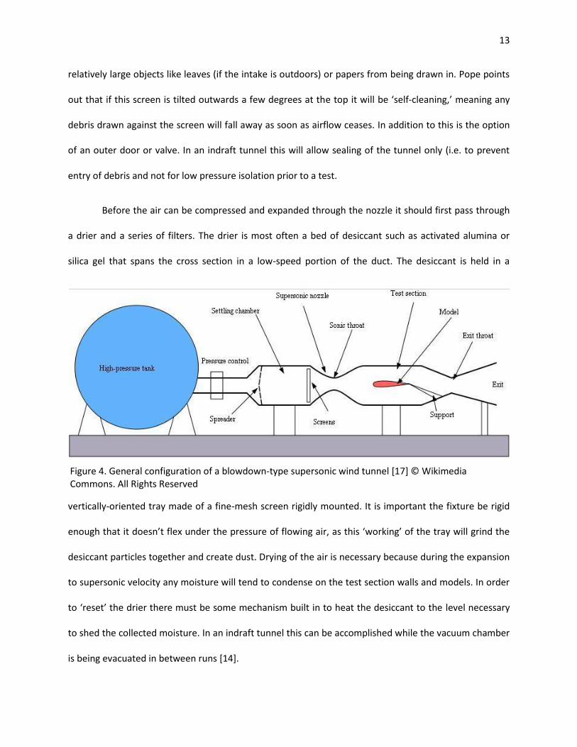
Figure 3 is a diagram of an indraft supersonic wind tunnel, as opposed to a blow-down tunnel

which is shown in Figure 4. At the opening of the tunnel there should be a screen or cage to keep

Figure 3. General configuration of an indraft-type supersonic wind tunnel.

13

relatively large objects like leaves (if the intake is outdoors) or papers from being drawn in. Pope points

out that if this screen is tilted outwards a few degrees at the top it will be ‘self-cleaning,’ meaning any

debris drawn against the screen will fall away as soon as airflow ceases. In addition to this is the option

of an outer door or valve. In an indraft tunnel this will allow sealing of the tunnel only (i.e. to prevent

entry of debris and not for low pressure isolation prior to a test.

Before the air can be compressed and expanded through the nozzle it should first pass through

a drier and a series of filters. The drier is most often a bed of desiccant such as activated alumina or

silica gel that spans the cross section in a low-speed portion of the duct. The desiccant is held in a

vertically-oriented tray made of a fine-mesh screen rigidly mounted. It is important the fixture be rigid

enough that it doesn’t flex under the pressure of flowing air, as this ‘working’ of the tray will grind the

desiccant particles together and create dust. Drying of the air is necessary because during the expansion

to supersonic velocity any moisture will tend to condense on the test section walls and models. In order

to ‘reset’ the drier there must be some mechanism built in to heat the desiccant to the level necessary

to shed the collected moisture. In an indraft tunnel this can be accomplished while the vacuum chamber

is being evacuated in between runs [14].

Figure 4. General configuration of a blowdown-type supersonic wind tunnel [17] © Wikimedia Commons. All Rights Reserved

14

There must also be a section where the airflow is filtered of particulates such as dust or oils, and

sent through directional vanes to promote steady, uniform flow. This section is called the settling

chamber. Velocity in this area should be no higher than 80 miles per hour (36 m/sec). The drier can be

included in this section but an advantage to keeping the drier in its own section is that it minimizes the

volume which must be heated when resetting the desiccant [14].

The de Laval-type convergent-divergent nozzle contains the first throat which chokes the flow.

When the first throat becomes choked the mass flow rate reaches a maximum that will be constant

throughout the duration of the run. The Mach number at a given point downstream of the throat can be

estimated using the area-Mach Number relation [2]. The area component is expressed as a

nondimensional ratio of the local duct cross-sectional area to the sonic throat cross-sectional area. The

test section area ratio determines the downstream Mach number for a particular test. Test sections in

general have relatively simple geometries in that they have a constant cross section, parallel walls and

thus constant cross-sectional area. However, multiple small orifices in the tunnel walls to accommodate

pressure transducers, the model mounting assembly, and the test section access window are also part of

the test section. Test sections can be configured in different ways depending on the speed regime. For

example, in supersonic testing the tunnel walls must be polished to minimize boundary layer turbulence,

but in transonic test sections the walls may be perforated or slotted. The number and type of pressure

sensors will vary according to the intended use of the tunnel. The model is mounted on a rod called the

sting. This is simply a connector with a known effect on the test data. The tunnel measurement

equipment must be calibrated with any auxiliary equipment that may be present which could skew test

results. A drive mechanism may be included in the mounting assembly. The drive mechanism may be

any variety as long as it provides fine control of pitch during model testing. This assembly must also

accommodate force and moment measuring devices. Mounting methods and analog measuring devices

are described in chapter 7 of Pope’s High Speed Wind Tunnel Testing [14].

15

A blow-down tunnel (Figure 4) has a similar configuration. In this case the pressure ratio comes

from a high-pressure tank upstream of the wind tunnel. Safety features are included in both designs

wherever appropriate, for example the test section access doors must be interlocked with the tunnel

control valves so that an operator is not harmed by an accidental flow startup.

Considering many SWTs have usable run times on the order of a few seconds, transient

inefficiencies can waste significant amounts of time. A 2009 paper by a group at the University of Texas

at Arlington’s Aerodynamics Research Center described the use of pre-programmed electronic

Proportional-Integral-Derivative controller (PID controller) to operate the isolation valve in blowdown

supersonic wind tunnels for the purpose of maximizing test time [10]. Using PID controllers to regulate

airflow is effective at preventing overshoot of stagnation pressure and thus limiting oscillations caused

by fast opening valves. As stagnation pressure is equal to

the ambient atmospheric pressure in an indraft

supersonic wind tunnel, this fine degree of control is not a

concern for the current project. For the current project

the tunnel run time is sufficiently lengthy that a slow,

manually operated valve will make the initial fluctuations that precede steady flow inconsequential.

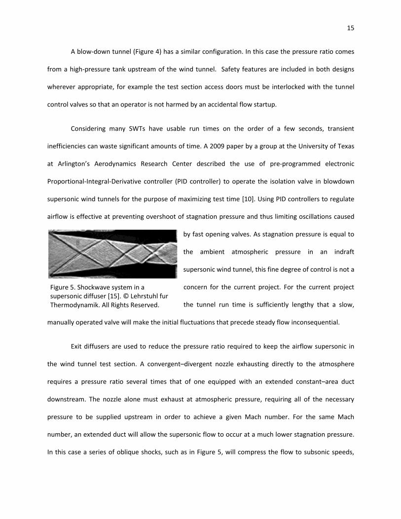
Exit diffusers are used to reduce the pressure ratio required to keep the airflow supersonic in

the wind tunnel test section. A convergent–divergent nozzle exhausting directly to the atmosphere

requires a pressure ratio several times that of one equipped with an extended constant–area duct

downstream. The nozzle alone must exhaust at atmospheric pressure, requiring all of the necessary

pressure to be supplied upstream in order to achieve a given Mach number. For the same Mach

number, an extended duct will allow the supersonic flow to occur at a much lower stagnation pressure.

In this case a series of oblique shocks, such as in Figure 5, will compress the flow to subsonic speeds,

Figure 5. Shockwave system in a supersonic diffuser [15]. © Lehrstuhl fur Thermodynamik. All Rights Reserved.

16

keeping the loss of stagnation pressure low while slowing the airflow. Therefore the pressure ratio

across the SWT is greatly reduced. Efficiency can be further improved by adding a diverging section at

the end of the tunnel to further slow the airflow. This configuration is called a normal shock diffuser.

Greater efficiency can be achieved using an oblique shock diffuser composed of a second, extended

region of smaller cross-sectional area relative to the throat downstream of the test section. The

converging geometry creates a series of reflecting oblique shocks which gradually slow the test section

Mach number until a weak normal shock at the end of this diffuser brings the flow to subsonic speed. A

divergent section continues to slow the flow and increase pressure. Oblique shock diffusers are always

less efficient in practice than they are in theory due to shock interaction with the viscous boundary

layers along the tunnel walls. It has been observed that the second throat cross-sectional area (At2)

required for choked flow at the first throat is less than that required to start the tunnel, and peak

efficiency is achieved by an At2 somewhere in between. This fact has led to the use of variable geometry

diffuser throats that constrict once the tunnel has been started [2].

The use of a diffuser in an indraft tunnel does not bring all of the advantages of a diffuser on a

blowdown tunnel [2]. Considering that the tunnel will be exhausting into a vacuum the flow will initially

be underexpanded and as the tank pressure rises will be overexpanded, and finally a shock will travel up

the test section to end the test. It is only during this last time interval, when the shocks form inside the

tunnel, that a diffuser would extend test time.

Other examples of recent research include studies of free-stream disturbance fields in SWTs

where experiments are conducted on laminar-turbulent transitions. These tunnels may have run times

measured in milliseconds [18]. Further studies have been conducted on control algorithms using

proportional-integral-differential (PID) controllers with variable throat nozzles to optimize test

conditions in blow-down tunnels [13]. Many questions remain concerning the laminar-turbulent

17

transition and shockwave-boundary layer interaction. Likewise, phenomena associated with the

transonic regime of airflow have been resistant to effective modeling and must be investigated through

experimentation [6].

The central object of most research and development efforts with respect to testing in the

supersonic regime has been greater accuracy and control over test conditions. Critical characteristics of

wind tunnel flow are Mach number, Reynolds number, pressures, and temperatures. Precise knowledge

and control of these variables in the test section allows for testing that better-reflects actual flight

conditions.

18

3. Summary of the Method of Characteristics

Characteristics are ‘lines’ in a supersonic flow oriented in specific directions along which

disturbances (pressure waves) are propagated. The Method of Characteristics (MOC) is a numerical

procedure appropriate for solving, among other things, two-dimensional compressible flow problems.

By using this technique, flow properties such as direction and velocity, can be calculated at distinct

points throughout a flow field. The method of characteristics, implemented in computer algorithms, is

an important element of supersonic computational fluid dynamics software. These calculations can be

executed manually, with the aid of spreadsheet programming or technical computing software (e.g.

Matlab or Mathematica). As the number of characteristic lines increase, so do the data points, and the

manual calculations can become exceedingly tedious.

James John and Theo Keith’s textbook, Gas Dynamics [9], describes three properties of

characteristics.

Property 1: A characteristic in a two-dimensional supersonic flow is a curve or line along which physical disturbances are propagated at the local speed of sound relative to the gas.

Property 2: A characteristic is a curve across which flow properties are continuous, although they may have discontinuous first derivatives, and along which the derivatives are indeterminate.

Property 3: A characteristic is a curve along which the governing partial differential equations(s) may be manipulated into an ordinary differential equation(s).

Property 1 is what dictates that characteristics are Mach lines. “Fluid particles travel along

pathlines propagating information regarding the condition of the flow... In supersonic flow, acoustic

waves travel along Mach lines (or characteristics) propagating information regarding flow disturbances”

[9].

19

Property 2 States that a Mach line

can be thought of as an infinitesimally thin

interface between two smooth and

uniform, but different regions. The line is a

boundary between continuous flows. Along

a streamline passing through a field of

these Mach waves, the derivative of the

velocity and other properties may be

discontinuous.

Property 3 essentially speaks for itself. It is important because ordinary differential equations

are often easier to solve than partial differential equations.

While the ratios of duct areas are relatively straightforward to determine based on desired test-

section Mach numbers and tunnel run times, determining an optimum channel contour is slightly more

complicated. It is in the region immediately after the sonic throat where the flow is turned away from

itself that the air expands into supersonic velocity. This expansion happens rather gradually over the

initial expansion region as seen in Figure 6. In

the Prandtl-Meyer expansion scenario, it is

assumed that the expansion takes place

across a centered fan originating from an

abrupt corner as in Figure 7. This

phenomenon is typically modeled as a

continuous series of expansion waves, each

turning the airflow an infinitesimal amount

Figure 6. Characteristic lines downstream of a supersonic throat

Figure 7. Expansion fan caused by supersonic airflow around a corner

20

along with the contour of the channel wall. These expansion waves can be thought of as the opposite of

shock compression waves, which slow airflow. This is governed by the Prandtl-Meyer function:

𝑑𝜃 = 𝑀2 − 1𝑑𝑉

𝑉

(1)

Where the change in flow angle (relative to its original direction) is represented by 𝑑𝜃. Eq. 1 integrates

to give the following (Equation (7.10) in [9]):

𝜈 𝑀 = 𝛾 + 1

𝛾 − 1tan−1

𝛾 − 1

𝛾 + 1(𝑀2 − 1) − tan−1 𝑀2 − 1

(2)

The parameter 𝜈 is known as the Prandtl-Meyer angle.

In MOC calculations, angles and other relations are in reference to the geometry shown in

Figure 8. Also in that figure is a diagram of the right-running characteristics from point ‘A’ and the left-

Figure 8. Geometry of characteristics at a point and impinging characteristics

21

running characteristics from point ‘B’ impinging on point P.

Method of Characteristics analysis for this project used the following equations; all taken from

chapter 14 of Gas Dynamics [9], and numbered as they appear in that text. In Method of Characteristics

equations the angle of the flow with respect to the horizontal is given the symbol α. The Mach angle μ is

defined as 𝜇 = sin−1 1

𝑀. The equations reference Figure 8,

𝑑𝑦

𝑑𝑥 𝐼

= tan(𝛼 − 𝜇)

14.43

𝑑𝑦

𝑑𝑥 𝐼𝐼

= tan(𝛼 + 𝜇)

14.44

𝜈 + 𝛼 = 𝑐𝑜𝑛𝑠𝑡𝑎𝑛𝑡 = 𝐶𝐼

14.56

𝜈 − 𝛼 = 𝑐𝑜𝑛𝑠𝑡𝑎𝑛𝑡 = 𝐶𝐼𝐼

14.57

The constants CI and CII are known as Riemann invariants.

𝜈𝑃 =𝐶𝐼 + 𝐶𝐼𝐼

2

14.58

𝛼𝑃 =𝐶𝐼 − 𝐶𝐼𝐼

2

14.59

22

𝑚𝐼 = tan 𝛼 − 𝜇 𝐴 + 𝛼 − 𝜇 𝑃

2

and

𝑚𝐼𝐼 = tan 𝛼 + 𝜇 𝐵 + 𝛼 + 𝜇 𝑃

2

14.60

𝑦𝑃 = 𝑦𝐴 + 𝑚𝐼 𝑥𝑃 − 𝑥𝐴

and

𝑦𝑃 = 𝑦𝐵 + 𝑚𝐼𝐼 𝑥𝑃 − 𝑥𝐵

14.61

𝑥𝑃 =𝑦𝐴 − 𝑦𝐵 + 𝑚𝐼𝐼𝑥𝐵 −𝑚𝐼𝑥𝐴

𝑚𝐼𝐼 −𝑚𝐼

14.62

A hand-drawn diagram of the “characteristic net” using pencil and ruler is a valuable aide to this

process. This will be referred back to as a reference of which points relate to each other, and what the

proper relations are. The first step in carrying out an analysis with this method is to choose the angle of

the expansion region. The assumption is that after an abrupt corner there will be an expansion region

with straight walls. The angle of the wall with respect to the horizontal centerline is the value of α at the

first point. Now choose how many characteristics will initially be used. It is convenient to choose an

amount of characteristics that will result in an even division of α. For example, if 𝛼 = 20° there could be

five characteristics at 20°, 15°, 10°, 5°, and 0°. These values would be set as the α-value for the first five

points which constitute an initial value line. The next four points are assumed to have α-values that split

those of the first five. In the case of the above example these will be 17.5°, 12.5°, 7.5°, and 2.5°.

23

Throughout the process the α-values will continue to follow this pattern with the exception of wall

points in the straightening region, which will be addressed when necessary.

An initial Mach number must be assumed for the five initial points. From this, using the Prandtl-

Meyer function, ν can be found, thus giving values for the Riemann invariants. Since the initial Mach

number is arbitrarily assumed, the Prandtl-Meyer function can be used for these points. That is the only

time the Mach number will be initially known. Additionally the initial group of coordinates can be found

by the Pythagorean Theorem and trigonometry. For the rest of the flow the Mach number (and the

coordinate points) must be derived. The Riemann invariants allow this to be accomplished. Equations

(14.58) and (14.59) define how α and ν can be found from CI and CII. After this in the analysis the Mach

number will be derived with the following equation, given in Example 7.1 in Gas Dynamics [9]:

𝑓 𝑀 = 𝛾 + 1

𝛾 − 1tan−1

𝛾 − 1

𝛾 + 1 𝑀2 − 1 − tan−1 𝑀2 − 1 − 𝜈

(3)

Using the goal seek feature in Microsoft Excel, for a given value of ν and γ, seek the value of M that sets

𝑓 𝑀 = 0. There is now enough information to find the slopes of each Riemann invariant. These are

found using the two equations labeled (14.60) and the point coordinates are determined by Equations

(14.61) and (14.62).

Next, select where the wall will begin to straighten. This point will have an α-value equal to that

of its ‘B’ point, referring to Figure 8. As the points are being mapped by hand on the diagram they will be

labeled appropriately. At this point in the analysis the inputs for the equations must be adjusted as

needed according to the characteristic net diagram. As the characteristics terminate against the wall

eventually the final one will lead to a final coordinate. This is the end point of the straightening section

and the beginning of the test section. The wind tunnel walls are now parallel. As this is a manual process

24

there may be some iteration required. If there are constraints, such as tunnel height or Mach number,

that are not being met it is necessary to change the first characteristic termination point. The Method of

Characteristics is not inherently iterative, but as this is an analytical procedure some trial and error must

be conducted.

25

4. Wind Tunnel Design, Fabrication, and Assembly

The practical objectives of this project, once the theory was understood and incorporated, were

to design, fabricate, and assemble a small working supersonic wind tunnel for laboratory use. The first

step was the establishment of several governing parameters. These are calculated using MATLAB (The

MathWorks Inc., Natick, MA) and the results are plotted below. The information yielded by these

calculations was used to settle on a design concept based on run time and test-section Mach number.

An optimum design for duct components and a vacuum chamber interface flange was then generated

using SolidWorks (Dassault Systèmes SolidWorks Corp., Concord, MA). Working within the budget

constraint, materials were obtained and sent to the Higgins Laboratories Manufacturing Shop for

fabrication of components.

4.1 Vacuum chamber and pump constraints

The WPI Vacuum Test Facility is a 50 inch by

72 inch, 35,343 cubic inch (2.3167 m3) vacuum

chamber, with supporting instrumentation. It is

pumped down by a combined rotary mechanical pump

and a positive displacement blower. This supplies a

pumping speed of over 10-2–10-3 Torr (560 liters per

second). The cycle time (the total time from the start

of one run to the equipment being ready for the next

run) of this apparatus is determined by the time required to pump down the vacuum chamber in

between tunnel runs. A vessel of volume V takes the following time to be pumped from Pi to Pf at a

given pumping speed S:

Figure 9. The WPI Vacuum Test Facility (VTF)

26

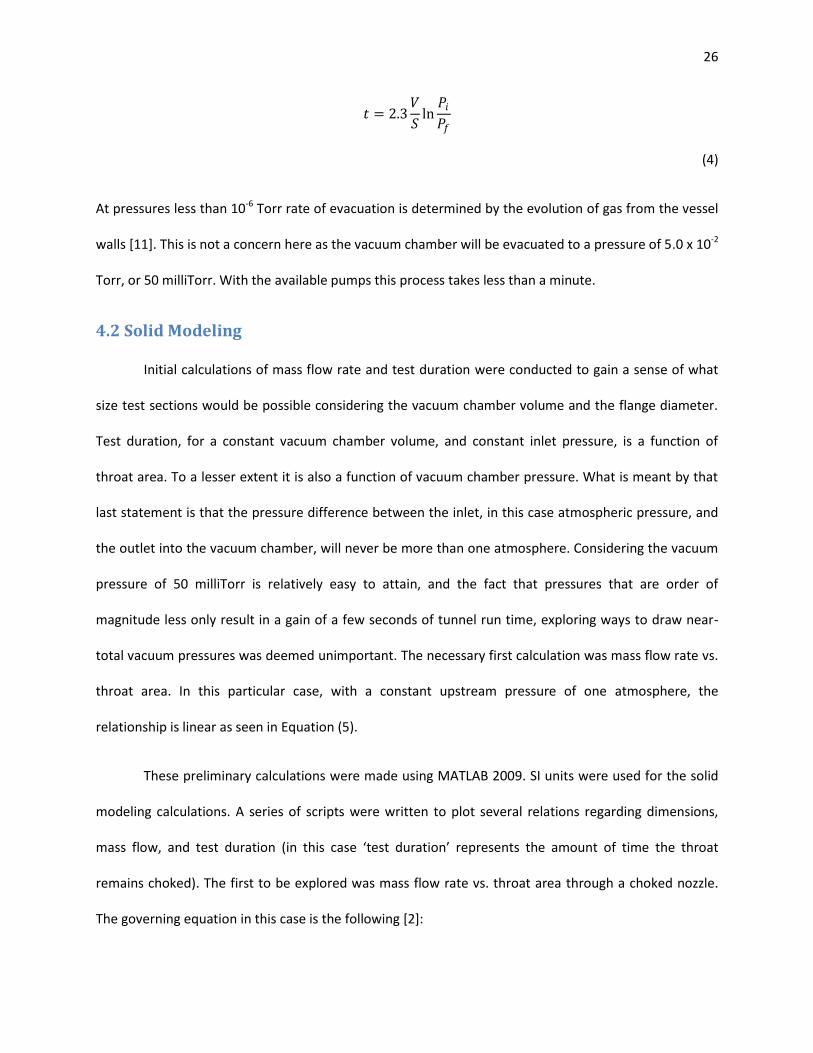
𝑡 = 2.3𝑉

𝑆ln𝑃𝑖𝑃𝑓

(4)

At pressures less than 10-6 Torr rate of evacuation is determined by the evolution of gas from the vessel

walls [11]. This is not a concern here as the vacuum chamber will be evacuated to a pressure of 5.0 x 10-2

Torr, or 50 milliTorr. With the available pumps this process takes less than a minute.

4.2 Solid Modeling

Initial calculations of mass flow rate and test duration were conducted to gain a sense of what

size test sections would be possible considering the vacuum chamber volume and the flange diameter.

Test duration, for a constant vacuum chamber volume, and constant inlet pressure, is a function of

throat area. To a lesser extent it is also a function of vacuum chamber pressure. What is meant by that

last statement is that the pressure difference between the inlet, in this case atmospheric pressure, and

the outlet into the vacuum chamber, will never be more than one atmosphere. Considering the vacuum

pressure of 50 milliTorr is relatively easy to attain, and the fact that pressures that are order of

magnitude less only result in a gain of a few seconds of tunnel run time, exploring ways to draw near-

total vacuum pressures was deemed unimportant. The necessary first calculation was mass flow rate vs.

throat area. In this particular case, with a constant upstream pressure of one atmosphere, the

relationship is linear as seen in Equation (5).

These preliminary calculations were made using MATLAB 2009. SI units were used for the solid

modeling calculations. A series of scripts were written to plot several relations regarding dimensions,

mass flow, and test duration (in this case ‘test duration’ represents the amount of time the throat

remains choked). The first to be explored was mass flow rate vs. throat area through a choked nozzle.

The governing equation in this case is the following [2]:

27

𝑚 = 𝑃𝑡𝐴

∗

𝑇𝑡

𝛾

𝑅

2

𝛾 + 1

𝛾+1𝛾−1

(5)

Once the throat of a converging-diverging nozzle becomes choked, mass flow rate will remain constant

until the nozzle unchokes. Specifically, for a constant back pressure at the tunnel exit, Pb, if the upstream

pressure, Pt, is at least equal to 1.8929Pb, the throat will choke and any further decrease in Pb will not

increase the mass flow rate through the nozzle.

As seen in Equation (5), there is a

linear relationship between mass

flow rate and throat area. The

resulting plot is shown in Figure 10.

For this calculation the following

values were assumed, γ = 1.4, R =

287 J/(kg*K), Tt = 293K, and Pt =

101325 Pa. As previously described,

indraft tunnels draw from the

ambient atmosphere, which is

reasonably assumed to be constant. By assuming isentropic conditions in the wind tunnel the stagnation

pressure (Pt) in the converging section of the nozzle is also constant, as is the stagnation temperature

(Tt). Should the tunnel be designed with the option to run continuously while evacuating the vacuum

chamber the mass flow rate through the throat must not exceed the capacity of the vacuum pump.

The next relation was test duration as a function of throat area. Test duration here is considered

the time from when the tunnel ‘starts,’ meaning the moment the throat becomes choked and the flow

Figure 10. Mass flow rate vs. throat area. Created in MATLAB, using Equation 5.

28

in the test section becomes supersonic, to when the pressure in the vacuum chamber becomes high

enough that the tunnel unchokes. The governing equation here is the following.

𝑡 = 𝑉𝑇𝑃𝑒𝑚 𝑅𝑇𝑡

1 −𝑃𝑖𝑃𝑒

(6)

Equation (6) is derived from the

continuity equation. The details of this

derivation are given Section 6.1 in the

appendix. The resulting plot is shown in

Figure 11.

Equation (6) introduces a new

ratio, 𝑃𝑖 𝑃𝑒 . This specifically is the ratio

of initial vacuum chamber pressure to

end-of-run vacuum chamber pressure.

𝑃𝑒 is found from the pressure ratio

required to sustain supersonic flow through the test section. The ratio of stagnation to static pressure at

a given Mach number is defined by Equation (3.30) in John D. Anderson’s Modern Compressible Flow [2].

It is repeated here:

𝑃𝑡𝑃

= 1 +𝛾 − 1

2𝑀2

𝛾𝛾−1

(7)

At the sonic condition M=1, Equation (6) reduces to the following, given as Equation (3.35) in Anderson

[2]:

Figure 11. Test duration vs. mass flow rate. Assumes isentropic conditions, initial vacuum chamber pressure Pi = 6.6875 Pa, and end of run chamber pressure Pe = 53499.6 Pa

29

𝑃∗

𝑃𝑡=

2

𝛾 + 1

𝛾𝛾−1

(8)

Note Equation (8) refers to the characteristic pressure at a sonic throat. Assuming that 𝛾 = 1.4,

𝑃∗ 𝑃𝑡 ≅ 0.528. Once the back pressure in the vacuum chamber has risen to 0.528𝑃𝑡 , which is equal to

53499.6 Pa, a shock will have formed inside the tunnel. At this time flow in the test section will be

assumed completely subsonic and the test will be over. Due to the geometry of a converging – diverging

nozzle, the characteristic pressure 𝑃∗ can be replaced with the end of run pressure 𝑃𝑒 . For an indraft

tunnel, drawing from an atmospheric pressure 𝑃𝑡 = 101325 Pa, the end of run pressure will be

𝑃𝑒 = 53499.6 Pa. It must be made clear that in the end-of-run condition the throat is still choked and a

standing normal shock is in the expansion section compressing the test section flow to subsonic

conditions. In fact, according to the subsonic entries of the Isentropic Flow Properties table in Modern

Compressible Flow [2] this throat will remain choked until the vacuum chamber reaches 𝑃 = 0.996𝑃𝑡 , or

100919.7 Pa.

As described in section 4.1 the vacuum system uses a Stokes model 1721-2 displacement pump

and blower combination. The mass flow capability of the pump is determined by the pump speed

(volumetric flow rate) at a given pressure. This information is provided by the pump manufacturer as a

“pumping speed curve.” The mass flow rate is equal to the product of the pumping speed and gas

density in the vacuum chamber (density being determined from the ideal gas law). The minimum

starting pressure is selected so as to prevent oil back-streaming from the pump into the chamber as a

result of molecular diffusion. This minimum starting pressure value is approximately 50 milliTorr. This

model more accurately reflects the probable usage of this supersonic wind tunnel, since the blower is

not intended for continuous use.

30

Test section Mach number is a function of area, specifically, the ratio of the test section cross-

sectional area to the throat cross-sectional area. The relation 𝑀 = 𝑓(𝐴

𝐴∗) is given by the following

equation.

𝐴

𝐴∗

2

=1

𝑀2 2

𝛾 + 1 1 +

𝛾 − 1

2𝑀2

𝛾+1𝛾−1

(9)

Equation (9) is known as the area-Mach

number relation [2, 8]. For example, for

a test section Mach number of 4

corresponds to an area ratio of 10.72.

Figure 12. Area-Mach relation for a choked supersonic nozzle. Created in MATLAB.

31

An equation for test time as a

function of throat height, for a

constant throat width can be found

by substituting Equation (5) into

Equation (6). Making the substitution,

setting 𝐴∗ = 𝑤ℎ∗ and simplifying

yields the following equation:

𝑡 =𝑉𝑡𝑃𝑒

𝑃𝑡𝑤ℎ∗ 𝑅𝛾

𝑇𝑡

2𝛾 + 1

𝛾+1𝛾−1

1 −𝑃𝑖𝑃𝑒

(10)

Test duration for a throat width of 3.81cm (1.5 in) and height ranging from 0.1 – 2 cm (0.039 – 0.787 in)

is shown in Figure 13. The following assumptions were made for the calculation: 𝛾 = 1.4, 𝑃𝑖 =

6.6875 𝑃𝑎, 𝑃𝑒 = 53499.6 𝑃𝑎, 𝑃𝑡 = 101325 𝑃𝑎, 𝑇𝑡 = 293 𝐾, 𝑉𝑡 = 2.317 𝑚3, and 𝑅 = 287.

Figure 13. Test duration vs. throat height. Created in MATLAB.

32

4.3 Mechanical Design

Design of the wind tunnel encompassed three primary components. The rectangular entry

flange, the tunnel contours, and the end piece (which includes the round-to-square cross-section

transition). The wind tunnel assembly also includes clear acrylic walls which are fixed to both sides of

the tunnel with epoxy.

4.3.1 Rectangular entry flange

The Rectangular entry flange got its name simply because the final configuration for the test

section was rectangular. The body of the flange must be

compatible with the window flange, which stays fixed to a port

on the vacuum chamber. The opening in the rectangular entry

point is simply a smooth continuation of test section geometry.

Originally this component was going to be located immediately

after the tunnel control ball valve, which would have been

mounted downstream of the test section. Ball valves are made

to fit round tubes, so this would have had a round opening.

Figure 15: rectangular entry flange

Figure 14: exploded view of tunnel assembly

33

Further complicating the design, a supersonic transition from

rectangle to round would have been required upstream of the

valve. It was determined that this complication would add too much

to fabrication demands, which could be avoided given a simple line-

up change. We decided that the control ball valve would be

mounted at the inlet, which allowed the test section to discharge

directly through the rectangle entry flange. This alteration

tremendously simplified the machining requirements.

Apart from the airflow channel, the rectangular entry flange

only serves to mount the tunnel to the vacuum chamber via

the window flange. On the front of the rectangular entry flange

(Figures 15 and 16) is a shallow face recessed 1/8 inch into

which a 1/16 inch gasket will be fitted. With the channel

securely mounted to the flange, the depth of the recess and

the thickness of the gasket were planned so that the channel

assembly is seated within the plane of the flange. This provides

additional alignment for the assembly. The assembly is mounted to the rectangular entry flange with

four ANSI 1/4 -28 socket head bolts.

The window flange (Figure 17) is already in existence, and has been used for other applications.

This project treats it as a standard piece of support equipment for the vacuum test facility. A SolidWorks

model of the existing window flange was provided for use by this MQP by a graduate student, Nick

Behlman.

Figure 17: window flange

Figure 16. Image of finished rectangular entry flange.

34

4.3.2 Nozzle and test-section assembly

Before the more complicated calculations associated with the expansion and straightening

region can be conducted, the basic expansion ratio must be chosen. This decision affects two critical

properties of the design: the test section Mach number, and the tunnel run time. Constraints on these

criteria come from the size of the vacuum chamber access ports and the affordability of ball valves. The

ball valve must have a cross-sectional area greater than the sonic throat; otherwise the ball valve would

choke. Any desired test section Mach number and tunnel run time would have to be evaluated with

respect to the size of ball valve needed to accommodate the flow.

It was known that airflow in the tunnel would be treated as two-dimensional, so width would

remain constant. Therefore the expansion ratio was reduced to a height ratio. What was left was to

determine a width, a throat height, and a test section height that would create a Mach number

somewhere in the range of 2 to 4, and a tunnel run time of sufficient length for observations to be

taken. Other factors driving these dimensions were the thickness of the acrylic panels and the amount of

material needing to be left in order to accommodate mounting screws.

The height ratio finally settled upon was 8:1. The height of the throat is 0.25 in (0.635 cm) and

the test section height is 2 in (5.08 cm). Choked flow through a tunnel with this expansion ratio will

create a supersonic flow of approximately Mach 3.677. For the starting conditions of the Vacuum Test

Facility, 35,343 cubic inches at a pressure of 50 milliTorr, and the throat dimensions of 0.25 inch by 1.5

inches, the tunnel will theoretically remain choked for over twenty seconds.

According to a mid-1960’s English Ministry of Aviation paper [10], a two-dimensional nozzle can

be divided into the following regions:

1. The contraction, where flow is subsonic

2. The throat, where flow achieves sonic conditions

35

3. An initial expansion region, where the slope of the contour increases up to its maximum value

4. The straightening region, where cross sectional area increases, while slope decreases to zero

5. The test section with uniform and parallel walls.

The contraction, or convergent portion of the nozzle, needs no specific contour that provides any great

advantage over another. This region can be designed simply to provide a smooth, subsonic transition

into the throat [1]. For the final design of this project, this section is a simple spline providing a smooth

transition from the upstream parallel section to the narrow throat. The length of the converging section

was arbitrarily set to 1 in (2.54 cm).

Determining expansion ratios and throat areas involved little calculation. The critical aspect of

tunnel design was the throat contour. This feature required significant study and calculation before a

proper design was achieved. In modern aerospace engineering this sort of problem is resolved with

computational fluid dynamics. This project utilized an analytical technique called the Method of

Characteristics which has been described. The specific iterative process will be elaborated on below.

Supersonic airflow in the test section must not only be at the desired Mach number, but must

also be uniform and parallel. Referring to Figure 18, regions 3 and 4 are designed to provide a relatively

long expansion. Region 3 is called a nonsimple region (according to McCabe [11]) where curved

characteristic lines (see section 3 for a discussion of characteristic lines) are reflected off the contours.

Region 4, which McCabe labels the ‘Busemann’ region [11], begins at the inflection point of the contour

Figure 18. Tunnel contour

36

and can be considered a simple region with straight characteristic lines. This region is designed to cancel

the reflected expansion waves. A wave incident on the contour wall in the straightening region will

terminate on the surface. This cancelling effect is achieved when the wall turns exactly to the turning

angle of the impinging mach wave incident on a plane surface. The streamlines passing through region 4

will be directed parallel to the top and bottom of the tunnel [10].

After the theoretical contour length (regions 2 through 4) have been calculated through the

Method of Characteristics, McCabe recommends increasing the channel length an additional 30% as a

rule of thumb to compensate for viscous effects [10].

Initial analysis begins at what is assumed to be the location of the expansion wave in the tunnel

throat. This location is actually an infinitesimal distance from the throat, where the Mach number is

arbitrarily assumed to be 1.1. The wall contour at this location is assumed to be straight and angled 24°

from the centerline. This is the expansion region. It is further assumed that the throat curvature and the

beginning of the expansion section is rather abrupt, and so the Prandtl-Meyer formula for an expansion

fan around a corner is used. The following discussion of how the tunnel contour was designed refers to

Figure 8 and the Method of Characteristics equations in Chapter 3

There are four initial characteristics in this analysis. The spreadsheet programmed for this is

shown in Section 6.3.3, and this description of the analytical process references that table of numbers.

All coordinate values are in inches, as this is the dimension used in the component drawings. Points 1

through 4 have their locations fixed by geometry. Assuming point 1 is at the throat, 1/8 inch above the

centerline, its y-coordinate will be equal to 0.125. By the Pythagorean Theorem, for a flow angle of 24°,

the x-coordinate will be 0.28. Thus the reference origin is located on the centerline, 0.28 inches

upstream of the tunnel throat. The four initial points are equidistant. Analysis begins with point 1 being

37

set to a flow angle of 24°. For points 2, 3, and 4, α=16°, 8°, and 0° respectively. Points 5, 6, and 7 have

α=20°, 12°, and 4° respectively. Throughout the expansion region this pattern is followed.

For the first four points, the Mach number is set to 1.1. Using this, the Prandtl-Meyer angle ν is

found. With values for α and ν, CI and CII can be found. The coordinates of points 1 – 4 are found using

trigonometry. What followed was an iterative process resulting in a set of coordinates mapping the

intersection of characteristics with the contour walls and with each other. Certain points and values are

known and must be manually entered. For example, points along the centerline will have flow angles

α=0 and y-coordinates equal to 0. During the course of this type of analysis it is extremely easy to

become confused so it is essential to use a simple diagram. This can be drawn by hand with the use of a

ruler. This will be referenced to ensure that the proper coordinates are related to each other as they

should be. In this case, during extensive spreadsheet debugging, the diagrams were invaluable. Through

the relations given in the above equations, and the assumption that the left running characteristic CII

from a given point P is equal to the impinging CII from the upstream point B, the spreadsheet was

Figure 19. Tunnel contours. Note the upper contour is in a pre-polished condition, lower contour is in an intermediate polished condition.

38

populated with data. The only manual operation was the calculation of local Mach numbers using the

Prandtl-Meyer angle ν. This was done by using the Microsoft Excel feature ‘Goal Seek.’

In the first iteration, the initial ‘guess’ for the start of the straightening region (the point of the

first cancelling characteristic) was point 50. The constraint on this process was the test section height.

The analysis must end with a straight wall one inch above the test-section centerline. This point was

given the same flow angle as the ‘B’ point upstream. Here the spreadsheet programming was heavily

manipulated and shaped according to the configuration of point numbers as laid out in the diagram. The

process was carried out until the final characteristic cancels on the tunnel wall. In this first iteration the

final y-value was over 1.5 inches, which was not acceptable, therefore the straightening section would

have to be started at an earlier point. A second iteration was carried out, starting the straightening

section at the immediate upstream point which, and then a third using the next upstream point.

In the third iteration the first point of the straightening region was point 43. As the theoretical

contour configuration was altered most of the spreadsheet cells would automatically update

accordingly. However, as the straightening region needed to be manually manipulated there was still a

significant amount of iteration required.

After some manipulation the coordinate values would appear to be reasonable; all numbers

were positive, there were no longer dramatic jumps in magnitudes. As a test of validity beyond this

simple sanity check, the points were plotted to give a visual reference. With this picture the remaining

unobvious errors were immediately apparent. Further debugging produced the correct contour

coordinates, yielding a 6-1/2 inch long expansion and straightening region.

Excluding the expansion and straightening regions, the design of this component was a simple

process. Having found the length of those nonsimple regions, the contour was designed using

SolidWorks. There were two options for applying the correct curvature in the solid model. First the wall

39

coordinates could be curve-fit to get an equation which SolidWorks would use to define a curve. This

was not desirable since the best curve fit was inaccurate to such a degree as to be visually obvious. The

second option was to import coordinate points to define the curve and simply define coincident mates

between end points. This second technique proved to be the best approach.

Apart from the expansion contour, which is determined by numerical analysis, different ideas

for the channel configuration were evaluated. This included various methods of attaching the assembly

to the end pieces, and different internal geometries.

4.3.3 End Piece and Control Ball Valve

Due to the rectangular cross section of the wind tunnel and the round cross section of the

control ball valve, a transitional section was required. This was incorporated into the end piece. On the

tunnel side there is a recessed face identical to the one on the rectangle entry flange, with a 1.5 in

(0.591 cm) square opening to match the tunnel inlet. The tunnel bolts into the end piece exactly the

same as it bolts into the rectangle entry flange. The particular depth of the bolt holes were chosen to

allow at least seven threads to be fully engaged. Both of these interfaces are designed to withstand an

atmosphere of pressure, as the tunnel will be under a vacuum until the valve is open. On the opposite

side is a round opening to accept the control valve. The transition from round to square was

accomplished by the SolidWorks chamfer and fillet functions. The main concern was to create a smooth

transition in order to minimize eddies and turbulence, so the angles and radii of the chamfers and fillets

are non-critical.

The circular opening is meant to accept a short length of copper tubing. As visible in Figure 20,

there is a narrow lip inside the opening. This is designed to provide as smooth of an internal surface as

possible. Due to the configuration of the ball valve body this copper pipe is necessary as a female-female

adapter. The valve, copper pipe, and end piece are joined together with metallic epoxy. Brazing was the

40

original plan for joining these components,

but this would have heated the Teflon ball

valve lining to such a degree that it would

likely suffer severe degradation.

After several ideas were discussed

and rejected by the author and Professor

Blandino, This design for the square to round

transition was arrived upon. The original

concept was for a much larger two-piece

assembly. This was strictly brainstorm material and was dismissed for a number of reasons, particularly

the fact that it would have been cast in a mold. It was in the last stages of the design process that the

decision was made to locate the transition in the upstream section of the tunnel. Originally this was

planned to be the last tunnel feature before airflow entered the vacuum chamber. One consideration in

moving this feature, and thus the control valve to the front of the tunnel was price. Ball valves increase

significantly in price according to their diameter. If the ball valve was located downstream of the test

section, minimizing the ball valve diameter

would have created a feature complicated

to machine. Most importantly, having a ball

valve downstream of the test section would

rule out the option of installing models that

are supported in the vacuum chamber.

Additionally, the entire weight of the test

section is supported by its interface with the

Figure 21. End piece, front and back

Figure 20. Finished end piece

41

vacuum chamber. The final configuration provides a much more robust mounting of the tunnel.

Figure 22. Completed tunnel parts. Note 12-inch ruler added for scale.

42

4.4 Material

The final duct, including channel contour pieces and end flanges was constructed of 6061

aluminum. This material was selected for its light weight, affordability, and easy machinability. The

window flange as designed by Nick Belman is made from stainless steel. The transparent walls of the

wind tunnel are 0.25 in (0.635 cm) thick extruded acrylic, bonded to the aluminum with epoxy. The

control valve is a 1½ inch manually operated brass ball valve with Teflon packing. It is secured to the end

piece via a copper adapter with a metal epoxy such as JB Weld (JB Weld Company). Gasket material is

1/8 in thick rubber sheet with a hardness of 35-45 as measured on the Durometer scale.

By attempting to stay within the project budget of $160.00 the necessary materials had to be

secured strategically. Several options were explored. Surplus aluminum in the required shapes and sizes

was not available from WPI machine shops, and the standard sizes in which these materials are sold

would have far exceeded the budget. Luckily several suppliers offered ‘scrap bin’ type sales, and leftover

pieces were available that suited the project requirements perfectly. Ultimately the project went over

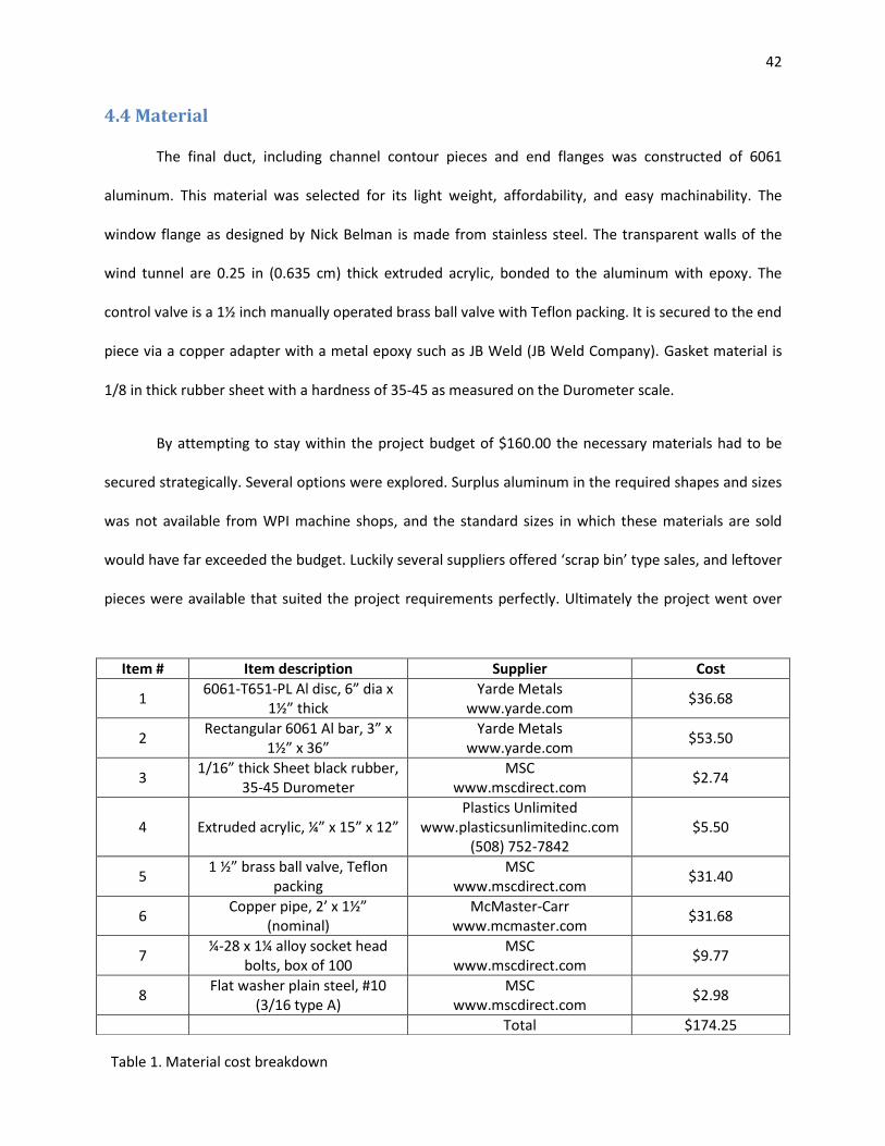
Table 1. Material cost breakdown

Item # Item description Supplier Cost

1 6061-T651-PL Al disc, 6” dia x

1½” thick Yarde Metals

www.yarde.com $36.68

2 Rectangular 6061 Al bar, 3” x

1½” x 36” Yarde Metals

www.yarde.com $53.50

3 1/16” thick Sheet black rubber,

35-45 Durometer MSC

www.mscdirect.com $2.74

4 Extruded acrylic, ¼” x 15” x 12” Plastics Unlimited

www.plasticsunlimitedinc.com (508) 752-7842

$5.50

5 1 ½” brass ball valve, Teflon

packing MSC

www.mscdirect.com $31.40

6 Copper pipe, 2’ x 1½”

(nominal) McMaster-Carr

www.mcmaster.com $31.68

7 ¼-28 x 1¼ alloy socket head

bolts, box of 100 MSC

www.mscdirect.com $9.77

8 Flat washer plain steel, #10

(3/16 type A) MSC

www.mscdirect.com $2.98

Total $174.25

43

budget by $14.25, which according to WPI official Barbara Furhman was acceptable.

The rectangular entry flange was fabricated from Item number 1, the end piece, and both

channel contours were fabricated from Item 2. Item 3 was cut into gaskets. Item 4 was used for the

windows. Item 5 is the control ball valve and Item 6 served as the female to female adapter for

mounting the valve to the tunnel. Items 7 and 8 were used to secure the two ends on the tunnel and

mount the tunnel onto the vacuum chamber via the stainless steel window flange.

4.5 Construction

All required materials have been obtained. Fabrication of the end piece, rectangle entry flange,

and two contours is complete with the exception of the final polishing of the contour walls as of October

20. Once the components have been finished the final assembly will be accomplished by the author.

Assembly will involve the following steps:

1. Cut copper pipe to appropriate length, such that when the ball valve is on one end and the other

is in the end piece the distance between the valve and end piece is only enough to comfortably

operate the ball valve handle.

2. Solder copper pipe inside ball valve such that the open position of the handle will be away from

the end piece.

3. Using a metallic epoxy such as JB Weld, fasten the other end of the copper pipe inside the end

piece. Align the ball valve handle in such a way that its operation will be along a vertical plane.

4. Cut the acrylic into two pieces such that there will be a small amount of overhang on either end

of the channel contour pieces.

5. Alignment of the acrylic tunnel walls is critical. To ensure the channel contours are aligned

properly and are the correct distance, bolt assembly together, stacking enough washers so that

the contours are not seated inside the shallow recesses of the end piece and rectangle entry

44

flange. Apply an appropriate epoxy to the contour sides and firmly press the acrylic walls against

the sides, leaving equal overhang on either end. Firmly clamp walls and let epoxy cure as

needed. When cured, remove tunnel from end piece and rectangle entry flange.

6. To ensure that the channel ends are flush and smooth, carefully remove any large pieces of

material with a band saw or mill, and then sand acrylic edges down until flush with aluminum.

7. Cut gasket material to proper size so that it will fit inside the two shallow recesses. Cut and trim

openings so that there are no obstructions in the air pathway once assembly is complete.

8. Insert gasket into the recessed face of the rectangle entry flange and bolt the downstream-side

of the tunnel into recess. Use one washer under the head of each bolt. Tighten gradually,

alternating between bolts so that the tunnel seats evenly on the gasket.

9. Repeat for the end piece. Bolt tunnel to end piece in the same manner.

This completes the assembly instructions of the supersonic wind tunnel. The next step is to mount

the tunnel on the WPI vacuum chamber via the window flange. The flange is designed to

accommodate an o-ring. It is anticipated that the seating surface on the rectangular entry flange will

create a sufficient seal with the window flange.

45

5. Conclusions

One of the original intentions of this project was to simulate and visualize the compressible

airflow throughout the tunnel using the Comsol Multiphysics software suite. Unfortunately it was soon

discovered that the current Comsol package does not support high speed compressible flow. The plan

was adapted to include numerical analysis of airflow via the Method of Characteristics. This proved to be

challenging. Familiarization with MOC involved the study of several example problems in Gas Dynamics

[9]. The results of those examples were combined and modified to generate an analysis tool in Microsoft

Excel. This tool, populated with data, and the accompanying plot of points is included in Appendix 6.3.3.

The academic exercise of learning MOC was a significant process in which a large amount of knowledge

was gained.

The work accomplished on this project during the summer of 2009 was the first step of a multi-

stage process. What has been accomplished will be presented to the next group. On September 8, 2009

a brief presentation of the mechanical design was made to the advisor Professor John Blandino, the co-

advisor Professor Simon Evans, and the students in the 2009-2010 MQP group. The slides are contained

in the appendix. At the conclusion of this project it is anticipated that the 2009-2010 MQP group will

partially incorporate this material into their work as needed.

There were many lengthy discussions between the author and the advisor about several issues

which were determined to be out of scope for this project. One is the treatment of the condensation

problem. Throughout the duration of choked flow, with the test section nominally at M=3.677, the static

pressure will be P=14.668 Torr (1955.57 Pa) and the static temperature will be T= -317°F (79K). It is

expected that upon starting the windows will immediately be covered with condensation. This is due to

the significant difference in static and stagnation pressures in the supersonic flow. At P=14.668 Torr and

T= -317°F, according to Table 18-2 in Physics for Scientists and Engineers [7], this is far above the

46

saturated vapor pressure of water. In spite of this, with concerns over time and budget, it was

determined that design of a drier would be beyond the scope of this project.

Also omitted from this design is a supersonic diffuser. When the tunnel starts the airflow will be

underexpanded as it enters the vacuum chamber. As the tank fills up, a point will be reached when the

flow is overexpanded, with oblique shocks downstream of the tunnel exit plane. Eventually, a normal

shock wave will be located at the tunnel exit plane. Without a supersonic diffuser, and with the uniform

cross sectional area, the normal shock will rapidly move through the test section to and into the throat.

The useable test time will have ended as soon as the shock moves into the test section since at that

point, despite the throat remaining choked; airflow in the test section will be subsonic.

Possible future work using this tunnel could involve the design of test equipment to directly

measure flow properties. A series of pressure taps could be added. A convenient way to accomplish this

could be the drilling of holes to allow microfluidics tubing, which would enable the measure of pressures

in-situ. Once the tunnel has been assembled, disassembly for any other major physical alteration may

not be possible. The groundwork that has been laid, with respect to methodology and solid modeling,

will be valuable as learning aids for students in the future.

A supersonic wind tunnel built for the testing of scale models is clearly a great deal more

complicated than this design, including driers, diffusers, model mounting and measuring equipment,

electronically controlled valves using PID systems, and even variable geometry throat and diffuser

contours. It would also need to be significantly larger. This small supersonic wind tunnel exhausts into

an 82 ft3 (2.317 m3) vacuum chamber and still only has a test duration of just over 20 seconds. An indraft

supersonic wind tunnel large enough to accommodate aircraft models would need an immense vacuum

chamber with a volume many times larger than what WPI is equipped with. In addition, as with any

project, limitations deriving from budgets and time constraints and manufacturing capabilities must be

47

grappled with. For example, given a larger budget and more time, a cartridge-type drier could be

incorporated into the wind tunnel inlet that could improve the anticipated condensation problem. Of

course, the fact is there will always be limits and there will always be trade-offs.

High speed wind tunnels equipped with the mentioned components and measurement systems

have helped to enable and hasten many of the technological advances in aerospace engineering of the

mid and late Twentieth Century. What this project has done is examine the essential feature required to

achieve steady, sustained supersonic flow. That feature is the nozzle contour. A profound appreciation

for the process by which that flow is made parallel and laminar has been gained.

48

6. Appendix

6.1 Test Duration: Derivation of Equation (6)

This derivation is started with the continuity equation; the volume of interest is that which undergoes a

pressure change. In the case of a blowdown wind tunnel this would be the upstream pressure vessel, or

for an indraft tunnel, such as this project, it is the vacuum chamber at the end of the duct. Specifically, in

this project, the volume represented here is that of the vacuum chamber. The process defined by

Equation (6) is assumed to be slow enough that stagnation temperature in the vacuum chamber remains

constant. What follows is a summary of the derivation of Equation (6) (Equation 3.4 in Pope [14]) by

Professor Blandino [5].

𝜕

𝜕𝑡 𝜌𝑑𝑉 = − 𝜌𝑽 ∙ 𝑑𝑨

(6.1.1)

Rearranged to equal zero,

𝜕

𝜕𝑡 𝜌𝑑𝑉 + 𝜌𝑽 ∙ 𝑑𝑨 = 0

(6.1.2)

For constant volume and duct throat cross-sectional area,

𝑑

𝑑𝑡 𝜌𝑉 + 𝜌𝑉𝐴 =

𝑑

𝑑𝑡 𝜌𝑉 + 𝑚 = 0

(6.1.3)

Stagnation density (or total density) is defined as the following,

𝜌𝑡 = 𝑃𝑡𝑅𝑇𝑡

(6.1.4)

49

From the governing equation for mass flow through a choked nozzle, the following equation relates

mass flow rate to the exit area. As defined previously, for a choked nozzle the mass flow rate through

the duct exit will be equal to that through the throat.

𝑚 = 𝑃𝑡𝐴

∗

𝑇𝑡

𝛾

𝑅

2

𝛾 + 1

𝛾+1𝛾−1

Equation (5)

This in turn equals

𝑚 = 𝜌𝑉𝐴∗ = 𝑃𝑡𝐴

∗

𝑇𝑡

𝛾

𝑅

2

𝛾 + 1

𝛾+1𝛾−1

(6.1.5)

For an indraft tunnel, Pt remains constant, so 𝑚 remains constant until throat is no longer choked.

Integrating Equation (6.1.3),

𝑉𝑇 𝑑𝜌𝑒

𝑖

= 𝑚 𝑑𝑡𝑡

0

(6.1.6)

For this derivation pressure and temperature will be the working properties instead of density. To

change the terms of Equation (6.1.6) to pressure we take a polytropic process of the form

𝑃𝑣𝑛 = 𝑐1

or

𝑃

𝜌𝑛= 𝑐2

Since we know initial conditions, 𝑝𝑖 ,𝜌𝑖 , we can equate

50

𝑃𝑖𝜌𝑖𝑛 =

𝑃

𝜌𝑛

In another form,

𝜌 𝑡 = 𝜌𝑖 𝑃 𝑡

𝑃𝑖

(6.1.7)

Differentiating Equation (6.1.7),

𝑑𝜌 =𝜌𝑖

𝑃𝑖

1𝑛 ∗

1

𝑛∗ 𝑃

1−𝑛𝑛 𝑑𝑃

(6.1.8)

Substitute (6.1.8) into (6.1.6),

𝑚 𝑡 = 𝑉𝑇𝜌𝑖𝑃𝑖

1

𝑛 𝑃

1−𝑛𝑛 𝑑𝑃

𝑒

𝑖

(6.1.9)

𝑚 𝑡 = 𝑉𝑇𝜌𝑖

𝑃𝑖

1𝑛 𝑃𝑒

1𝑛 1 −

𝑃𝑖𝑃𝑒

1𝑛

(6.1.10)

Since

𝑃𝑖𝜌𝑖𝑛 =

𝑃

𝜌𝑛

Equation (6.1.10) can be written as,

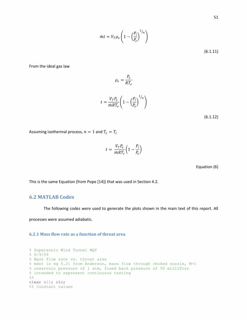
51

𝑚 𝑡 = 𝑉𝑇𝜌𝑒 1 − 𝑃𝑖𝑃𝑒

1𝑛

(6.1.11)

From the ideal gas law

𝜌𝑒 =𝑃𝑒𝑅𝑇𝑒

𝑡 =𝑉𝑇𝑃𝑒𝑚 𝑅𝑇𝑒

1 − 𝑃𝑖𝑃𝑒

1𝑛

(6.1.12)

Assuming isothermal process, 𝑛 = 1 and 𝑇𝑒 = 𝑇𝑡

𝑡 = 𝑉𝑇𝑃𝑒𝑚 𝑅𝑇𝑡

1 −𝑃𝑖𝑃𝑒

Equation (6)

This is the same Equation (from Pope [14]) that was used in Section 4.2.

6.2 MATLAB Codes

The following codes were used to generate the plots shown in the main text of this report. All

processes were assumed adiabatic.

6.2.1 Mass flow rate as a function of throat area

% Supersonic Wind Tunnel MQP % 6/9/09 % Mass flow rate vs. throat area % mdot is eq 5.21 from Anderson, mass flow through choked nozzle, M=1 % reservoir pressure of 1 atm, fixed back pressure of 50 milliTorr % intended to represent continuous testing %% clear all; clc; %% Constant values

52

gam = 1.4; % assumed ideal gas To = 293; % Kelvin, stagnation temperature of ambient air Po = 101325; % Pascals, stagnation pressure of ambient air R = 287; % J/(kg*K), gas constant for air at stp %% figure A = 1: 0.2: 9; % cm^2, cross sectional area of throat mdot = (A/10000)*Po/sqrt(To)*sqrt(gam/R*(2/(gam+1)^((gam+1)/(gam-1)))); % mass flow rate at throat plot(A,mdot); xlabel('throat area, cm^2'); ylabel('mass flow rate, kg/sec'); %% % A and Mdot are linearly related

6.2.2 Test Duration vs. Mass Flow Rate

function t=DurvsAthroat(Pi,mdot) % Supersonic Wind Tunnel MQP % 6/12/09 % Test duration vs. throat area % "test duration" is the amount of time from when air starts flowing until % the tunnel unchokes. It is a function of mass flow rate, which is a % function of throat area. % process is assumed adiabatic %% constant values

Pe = 53499.6; % Pa, pressure in vacuum chamber at end of run Tt = 293; % K, stagnation temp of atmosphere V = 2.317; % m^3, volume of vacuum chamber R = 287; % J/(kg*K), gas constant %%

t = (V*Pe./(mdot*R*Tt))*(1-Pi/Pe); % test duration

______________________________________________ %% Main file % Supersonic Wind Tunnel MQP % 6/12/09 % Test duration vs. throat area % "test duration" is the amount of time from when air starts flowing until % the tunnel unchokes. It is a function of mass flow rate, which is a % function of throat area. % process is assumed adiabatic %% clear; close; clc; Pi=6.68745; % Pa, initial pressure of pumped-down vacuum chamber mdot=0: 0.001: 0.04; % kg/sec mass flow rate

figure

for i=1:length(Pi) [t]=DurvsAthroat(Pi(i), mdot);

53

plot(mdot,t); hold on end legend(num2str(Pi')) xlabel('mass flow rate, kg/sec'); ylabel('test duration, sec')

6.2.3 Area-Mach number relation

%% Supersonic Wind Tunnel MQP % 6/22/09 % Area-Mach number relation % Plot of mach number vs. exit : throat area ratio %% clear; close; clc; gam = 1.4; % constant M = 1: 0.2: 5; % Range of mach numbers

figure

Ar = sqrt((1./M.^2).*(2/(gam+1)*(1+((gam-1)*M.^2)/2)).^((gam+1)/(gam-1)));

plot(Ar,M); xlabel('Area ratio A/A*'); ylabel('Mach number M');

6.2.4 Test Duration vs. Throat Height

% Supersonic Wind Tunnel MQP % 10/20/09 % Test duration vs. throat height %% clear all; clc; %% Constant values

gam = 1.4; % assumed ideal gas Tt = 293; % Kelvin, stagnation temperature of ambient air Pt = 101325; % Pascals, stagnation pressure of ambient air R = 287; % J/(kg*K), gas constant for air at stp w = 3.81; % cm, width of throat Pi = 6.6875; % Pa, initial pressure of pumped-down vacuum chamber Pe = 53499.6; % Pa, pressure in vacuum chamber at end of run V = 2.317; % m^3, volume of vacuum chamber %% figure h = 0.1: 0.1: 2; % cm, height of throat t = V*Pe*(1-Pi/Pe)./(Pt*w.*h*sqrt((R*gam/Tt)*(2/(gam+1))^((gam+1)/(gam-1)))); % test duration: time from start until tunnel unchokes plot(h,t); xlabel('throat height, cm'); ylabel('test duration, sec');

54

6.3 Method of Characteristics Spreadsheets

Analysis of the characteristic lines in the diverging and straightening sections of the channel contour was

conducted using Microsoft Excel 2007. The first step was an academic exercise intended to familiarize

the author with the procedure.

6.3.1 Key Assumptions and Parameters

The spreadsheet tools were created with similar assumptions and parameters as those

described in Chapter 3. They are as follows:

1. The initial Mach number is arbitrarily chosen to be greater than 1.

2. 4 characteristics, forming an initial value line, would be used.

3. The “second value line” would be the three intersections of the initial value line characteristics.

The α-value of these points would bisect the average of the two upstream points and so on.

4. The walls in the expansion region are straight and at an assumed angle.

6.3.2 Familiarization

Table 2 is a continuation of example 14.3 from John and Keith’s Gas Dynamics. Example 14.3 involves

the use of MOC to derive point coordinates for the characteristic net. Once that had been accomplished

the example was blended with a modified version of the following example 14.5 which derives

coordinates of points along the straightening region. Rows of the wall coordinates are tan colored for

identification. The wall of the straightening region is at a 6° angle to the horizontal.

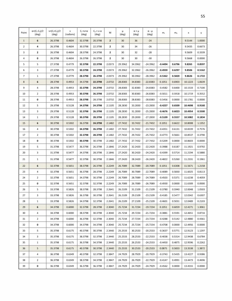
55

Point α=(CI-CII)/2

(deg) ν=(CI+CII)/2

(deg) ν

(radians) CI =ν+α (deg)

CII = ν-α (deg)

M μ

(deg) α + μ (deg)

α - μ (deg)

mI mII x y

1 6 26.3798 0.4604 32.3798 20.3798 2 30 36 -24 9.5144 1.0000

2 4 26.3798 0.4604 30.3798 22.3798 2 30 34 -26 9.5435 0.6673

3 2 26.3798 0.4604 28.3798 24.3798 2 30 32 -28 9.5609 0.3339

4 0 26.3798 0.4604 26.3798 26.3798 2 30 30 -30 9.5668 0.0000

5 5 27.3798 0.4779 32.3798 22.3798 2.0373 29.3962 34.3962 -24.3962 -0.4494 0.6796 9.8265 0.8597

6 3 27.3798 0.4779 30.3798 24.3798 2.0373 29.3962 32.3962 -26.3962 -0.4920 0.6297 9.8506 0.5162

7 1 27.3798 0.4779 28.3798 26.3798 2.0373 29.3962 30.3962 -28.3962 -0.5362 0.5820 9.8626 0.1722

8 6 28.3798 0.4953 34.3798 22.3798 2.0732 28.8383 34.8383 -22.8383 0.1051 0.6903 10.1223 1.0639

9 4 28.3798 0.4953 32.3798 24.3798 2.0732 28.8383 32.8383 -24.8383 -0.4582 0.6400 10.1533 0.7100

10 2 28.3798 0.4953 30.3798 26.3798 2.0732 28.8383 30.8383 -26.8383 -0.5011 0.5918 10.1719 0.3552

11 0 28.3798 0.4953 28.3798 28.3798 2.0732 28.8383 28.8383 -28.8383 -0.5456 0.0000 10.1781 0.0000

12 5 29.3798 0.5128 34.3798 24.3798 2.1105 28.2830 33.2830 -23.2830 -0.4257 0.6509 10.4698 0.9160

13 3 29.3798 0.5128 32.3798 26.3798 2.1105 28.2830 31.2830 -25.2830 -0.4676 0.6023 10.4954 0.5500

14 1 29.3798 0.5128 30.3798 28.3798 2.1105 28.2830 29.2830 -27.2830 -0.5109 0.5557 10.5082 0.1834

15 6 30.3798 0.5302 36.3798 24.3798 2.1482 27.7432 33.7432 -21.7432 0.1051 0.6622 10.8008 1.1352

16 4 30.3798 0.5302 34.3798 26.3798 2.1482 27.7432 31.7432 -23.7432 -0.4351 0.6131 10.8339 0.7576

17 2 30.3798 0.5302 32.3798 28.3798 2.1482 27.7432 29.7432 -25.7432 -0.4773 0.5661 10.8537 0.3790

18 0 30.3798 0.5302 30.3798 30.3798 2.1482 27.7432 27.7432 -27.7432 -0.5209 0.0000 10.8603 0.0000

19 5 31.3798 0.5477 36.3798 26.3798 2.1846 27.2420 32.2420 -22.2420 -0.3988 0.6187 11.1921 0.9792

20 3 31.3798 0.5477 34.3798 28.3798 2.1846 27.2420 30.2420 -24.2420 -0.4399 0.5714 11.2194 0.5880

21 1 31.3798 0.5477 32.3798 30.3798 2.1846 27.2420 28.2420 -26.2420 -0.4822 0.5260 11.2331 0.1961

22 6 32.3798 0.5651 38.3798 26.3798 2.2249 26.7089 32.7089 -20.7089 0.1051 0.6308 11.5671 1.2158

23 4 32.3798 0.5651 36.3798 28.3798 2.2249 26.7089 30.7089 -22.7089 -0.4089 0.5830 11.6025 0.8113

24 2 32.3798 0.5651 34.3798 30.3798 2.2249 26.7089 28.7089 -24.7089 -0.4503 0.5371 11.6238 0.4059

25 0 32.3798 0.5651 32.3798 32.3798 2.2249 26.7089 26.7089 -26.7089 -0.4930 0.0000 11.6309 0.0000

26 5 33.3798 0.5826 38.3798 28.3798 2.2641 26.2109 31.2109 -21.2109 -0.3780 0.5940 12.0048 1.0503

27 3 33.3798 0.5826 36.3798 30.3798 2.2641 26.2109 29.2109 -23.2109 -0.4185 0.5477 12.0342 0.6307

28 1 33.3798 0.5826 34.3798 32.3798 2.2641 26.2109 27.2109 -25.2109 -0.4601 0.5031 12.0489 0.2103

29 6 34.3798 0.6000 32.3798 28.3798 2.3040 25.7234 31.7234 -19.7234 0.1051 0.6059 12.4271 1.3061

30 4 34.3798 0.6000 38.3798 30.3798 2.3040 25.7234 29.7234 -21.7234 -0.3881 0.5591 12.4651 0.8716

31 2 34.3798 0.6000 36.3798 32.3798 2.3040 25.7234 27.7234 -23.7234 -0.4288 0.5142 12.4880 0.4361

32 0 34.3798 0.6000 34.3798 34.3798 2.3040 25.7234 25.7234 -25.7234 -0.4708 0.0000 12.4956 0.0000

33 5 35.3798 0.6175 40.3798 30.3798 2.3440 25.2533 30.2533 -20.2533 -0.3637 0.5771 12.9123 1.1297

34 3 35.3798 0.6175 38.3798 32.3798 2.3440 25.2533 28.2533 -22.2533 -0.4038 0.5314 12.9438 0.6784

35 1 35.3798 0.6175 36.3798 34.3798 2.3440 25.2533 26.2533 -24.2533 -0.4450 0.4875 12.9596 0.2262

36 5 35.3798 0.6175 40.3798 30.3798 2.3440 25.2533 30.2533 -20.2533 0.0875 0.5833 13.3538 1.3872

37 4 36.3798 0.6349 40.3798 32.3798 2.3847 24.7929 28.7929 -20.7929 -0.3743 0.5435 13.4227 0.9386

38 2 36.3798 0.6349 38.3798 34.3798 2.3847 24.7929 26.7929 -22.7929 -0.4147 0.4991 13.4473 0.4696

39 0 36.3798 0.6349 36.3798 36.3798 2.3847 24.7929 24.7929 -24.7929 -0.4562 0.0000 13.4555 0.0000

56

Point α=(CI-CII)/2

(deg) ν=(CI+CII)/2

(deg) ν

(radians) CI =ν+α (deg)

CII = ν-α (deg)

M μ

(deg) α + μ (deg)

α - μ (deg)

mI mII x Y

40 3 37.3798 0.6524 40.3798 34.3798 2.4262 24.3410 27.3410 -21.3410 -0.3852 0.5332 13.9476 0.7364

41 1 37.3798 0.6524 38.3798 36.3798 2.4262 24.3410 25.3410 -23.3410 -0.4259 0.4677 13.9771 0.2440

42 4 36.3798 0.6349 40.3798 32.3798 2.3849 24.7907 28.7907 -20.7907 0.0699 0.5496 14.3680 1.4581

43 2 38.3798 0.6699 40.3798 36.3798 2.4683 23.8997 25.8997 -21.8997 -0.3963 0.4796 14.5259 0.5072

44 0 38.3798 0.6699 38.3798 38.3798 2.4683 23.8997 23.8997 -23.8997 -0.4373 0.0000 14.5349 0.0000

45 1 39.3798 0.6873 40.3798 38.3798 2.5108 23.4707 24.4707 -22.4707 -0.4078 0.4491 15.1225 0.2639

46 3 37.3798 0.6524 40.3798 34.3798 2.4262 24.3410 27.3410 -21.3410 0.0524 0.5170 15.4536 1.5150

47 0 40.3798 0.7048 40.3798 40.3798 2.5543 23.0477 23.0477 -23.0477 -0.4195 0.0000 15.7516 0.0000

48 2 38.3798 0.6699 40.3798 36.3798 2.4683 23.8997 25.8997 -21.8997 0.0349 0.4856 16.6905 1.5582

49 1 39.3798 0.6873 40.3798 38.3798 2.5101 23.4776 24.4776 -22.4776 0.0175 0.4552 18.0170 1.5814

50 0 40.3798 0.7048 40.3798 40.3798 2.5543 23.0477 23.0477 -23.0477 0.0000 0.4255 19.4685 1.5814

Table 2. Analysis spreadsheet for familiarization with the Method of Characteristics

Figure 23. Plot of coordinate points of hypothetical expansion and straightening region derived in Table 2 for the familiarization example.

0

0.5

1

1.5

2

9 11 13 15 17 19

57

6.3.3 Wind tunnel diverging and straightening contour analysis

In this case the straightening wall is assumed to be 24° from the horizontal. The initial Mach

number at the assumed “throat” is assumed to be 1.1.

Point α=(CI-CII)/2

(deg) ν=(CI+CII)/2

(deg) ν

(radians) CI =ν+α (deg)

CII = ν-α (deg)

M μ

(deg) α + μ (deg)

α - μ (deg)

mI mII x y

1 24 1.3350 0.0233 25.3350 -22.6650 1.1 65.3800 89.3800 -41.3800 0.2800 0.1250

2 16 1.3350 0.0233 17.3350 -14.6650 1.1 65.3800 81.3800 -49.3800 0.2948 0.0845

3 8 1.3350 0.0233 9.3350 -6.6650 1.1 65.3800 73.3800 -57.3800 0.3037 0.0427

4 0 1.3350 0.0233 1.3350 1.3350 1.1 65.3800 65.3800 -65.3800 0.3066 0.0000

5 20 5.3350 0.0931 25.3350 -14.6650 1.2690 52.0011 72.0011 -32.0011 -

0.7451 4.2272 0.3007 0.1096

6 12 5.3350 0.0931 17.3350 -6.6650 1.2690 52.0011 64.0011 -40.0011 -

0.9893 2.5636 0.3130 0.0665

7 4 5.3350 0.0931 9.3350 1.3350 1.2690 52.0011 56.0011 -48.0011 -

1.3122 1.7813 0.3192 0.0223

8 24 9.3350 0.1629 33.3350 -14.6650 1.4121 45.0858 69.0858 -21.0858 0.4452 2.8307 0.3110 0.1388

9 16 9.3350 0.1629 25.3350 -6.6650 1.4121 45.0858 61.0858 -29.0858 -0.5901 1.9245 0.3272 0.0939

10 8 9.3350 0.1629 17.3350 1.3350 1.4121 45.0858 53.0858 -37.0858 -0.7967 1.4042 0.3370 0.0474

11 0 9.3350 0.1629 9.3350 9.3350 1.4121 45.0858 45.0858 -45.0858 -1.0554 0.0000 0.3403 0.0000

12 20 13.3350 0.2327 33.3350 -6.6650 1.5500 40.1778 60.1778 -20.1778 -

0.3765 1.7770 0.3452 0.1259

13 12 13.3350 0.2327 25.3350 1.3350 1.5500 40.1778 52.1778 -28.1778 -

0.5459 1.3095 0.3592 0.0765

14 4 13.3350 0.2327 17.3350 9.3350 1.5500 40.1778 44.1778 -36.1778 -

0.7435 0.9872 0.3663 0.0256

15 24 17.3350 0.3026 41.3350 -6.6650 1.6838 36.4339 60.4339 -12.4339 0.4452 1.7536 0.3667 0.1636

16 16 17.3350 0.3026 33.3350 1.3350 1.6838 36.4339 52.4339 -20.4339 -0.3700 1.2941 0.3858 0.1109

17 8 17.3350 0.3026 25.3350 9.3350 1.6838 36.4339 44.4339 -28.4339 -0.5386 0.9761 0.3973 0.0559

18 0 17.3350 0.3026 17.3350 17.3350 1.6838 36.4339 36.4339 -36.4339 -0.7347 0.0000 0.4011 0.0000

19 20 21.3350 0.3724 41.3350 1.3350 1.8200 33.3293 53.3293 -13.3293 -0.2287 1.3214 0.4170 0.1521

20 12 21.3350 0.3724 33.3350 9.3350 1.8200 33.3293 45.3293 -21.3293 -0.3815 0.9959 0.4340 0.0925

21 4 21.3350 0.3724 25.3350 17.3350 1.8200 33.3293 37.3293 -29.3293 -0.5516 0.7503 0.4425 0.0310

22 24 25.3350 0.4422 49.3350 1.3350 1.9604 30.6705 54.6705 -6.6705 0.4452 1.3764 0.4534 0.2022

23 16 25.3350 0.4422 41.3350 9.3350 1.9604 30.6705 46.6705 -14.6705 -0.2493 1.0355 0.4771 0.1371

24 8 25.3350 0.4422 33.3350 17.3350 1.9604 30.6705 38.6705 -22.6705 -0.4040 0.7813 0.4915 0.0693

25 0 25.3350 0.4422 25.3350 25.3350 1.9604 30.6705 30.6705 -30.6705 -0.5773 0.0000 0.4962 0.0000

26 20 29.3350 0.5120 49.3350 9.3350 2.1089 28.3060 48.3060 -8.3060 -0.1314 1.0909 0.5278 0.1924

27 12 29.3350 0.5120 41.3350 17.3350 2.1089 28.3060 40.3060 -16.3060 -0.2771 0.8240 0.5494 0.1171

28 4 29.3350 0.5120 33.3350 25.3350 2.1089 28.3060 32.3060 -24.3060 -0.4346 0.6125 0.5604 0.0393

29 24 33.3350 0.5818 57.3350 9.3350 2.2624 26.2321 50.2321 -2.2321 0.4452 1.1613 0.5878 0.2620

30 16 33.3350 0.5818 49.3350 17.3350 2.2624 26.2321 42.2321 -10.2321 -0.1632 0.8776 0.6184 0.1776

31 8 33.3350 0.5818 41.3350 25.3350 2.2624 26.2321 34.2321 -18.2321 -0.3109 0.6561 0.6373 0.0897

32 0 33.3350 0.5818 33.3350 33.3350 2.2624 26.2321 26.2321 -26.2321 -0.4720 0.0000 0.6438 0.0000

33 20 37.3350 0.6516 57.3350 17.3350 2.4314 24.2856 44.2856 -4.2856 -0.0569 0.9410 0.7012 0.2556

34 12 37.3350 0.6516 49.3350 25.3350 2.4314 24.2856 36.2856 -12.2856 -0.1991 0.7070 0.7302 0.1554

35 4 37.3350 0.6516 41.3350 33.3350 2.4314 24.2856 28.2856 -20.2856 -0.3494 0.5152 0.7449 0.0521

58

Point α=(CI-CII)/2

(deg) ν=(CI+CII)/2

(deg) ν

(radians) CI =ν+α (deg)

CII = ν-α (deg)

M μ

(deg) α + μ (deg)

α - μ (deg)

mI mII x y

36 24 41.3350 0.7214 65.3350 17.3350 2.5963 22.6539 46.6539 1.3461 0.4452 1.0165 0.8010 0.3570

37 16 41.3350 0.7214 57.3350 25.3350 2.5963 22.6539 38.6539 -6.6539 -0.0958 0.7665 0.8431 0.2420

38 8 41.3350 0.7214 49.3350 33.3350 2.5963 22.6539 30.6539 -14.6539 -0.2395 0.5651 0.8689 0.1222

39 0 41.3350 0.7214 41.3350 36.3798 2.5963 22.6539 22.6539 -22.6539 -0.3933 0.0000 0.8775 0.0000

40 20 45.3350 0.7912 57.3350 33.3350 2.7801 21.0817 41.0817 -1.0817 0.0023 0.8352 0.9813 0.3574

41 12 45.3350 0.7912 49.3350 41.3350 2.7801 21.0817 33.0817 -9.0817 -0.1382 0.6217 1.0219 0.2173

42 4 45.3350 0.7912 49.3350 25.3350 2.7801 21.0817 25.0817 -17.0817 -0.2843 0.4425 1.0422 0.0729

43 20 45.3350 0.7912 65.3350 25.3350 2.7801 21.0817 41.0817 -1.0817 0.3640 0.8718 1.1097 0.4693

44 16 49.3350 0.8611 65.3350 33.3350 2.9781 19.6203 35.6203 -3.6203 -0.0411 0.6835 1.2130 0.3479

45 8 49.3350 0.8611 57.3350 41.3350 2.9781 19.6203 27.6203 -11.6203 -0.1827 0.4953 1.2497 0.1757

46 0 49.3350 0.8611 49.3350 49.3350 2.9781 19.6203 19.6203 -19.6203 -0.3317 0.0000 1.2620 0.0000

47 12 53.3350 0.9309 65.3350 41.3350 3.1929 18.2519 30.2519 -6.2519 -0.0864 0.5529 1.5141 0.3219

48 4 53.3350 0.9309 57.3350 49.3350 3.1929 18.2519 22.2519 -14.2519 -0.2297 0.3826 1.5443 0.1080

49 8 57.3350 1.0007 65.3350 49.3350 3.4262 16.9699 24.9699 -8.9699 -0.1336 0.4371 1.9120 0.2687

50 0 57.3350 1.0007 57.3350 57.3350 3.4262 16.9699 16.9699 -16.9699 -0.2794 0.0000 1.9308 0.0000

51 16 49.3350 0.8611 65.3350 33.3350 2.9781 19.6203 35.6203 -3.6203 0.2867 0.7165 1.5645 0.5997

52 4 61.3350 1.0705 65.3350 57.3350 3.6820 15.7590 19.7590 -11.7590 -0.1829 0.3320 2.4460 0.1710

53 12 53.3350 0.9309 65.3350 41.3350 3.1923 18.2554 30.2554 -6.2554 0.2126 0.5833 2.2348 0.7422

54 0 65.3350 1.1403 65.3350 65.3350 3.9655 14.6063 14.6063 -14.6063 -0.2342 0.0000 3.1762 0.0000

55 8 57.3350 1.0007 65.3350 49.3350 3.4262 16.9699 24.9699 -8.9699 0.1405 0.4657 3.2288 0.8819

56 4 61.3350 1.0705 65.3350 57.3350 3.6820 15.7590 19.7590 -11.7590 0.0699 0.3592 4.7141 0.9858

57 0 65.3350 1.1403 65.3350 65.3350 3.9655 14.6063 14.6063 -14.6063 0.0000 0.2606 6.9589 0.9858

Table 3. Method of characteristics analysis table for wind tunnel contour

The final Mach number according to this table is M=3.9655. The final height is 0.9858 in.

Contrast this with the design area ratio of 8, with (according to 1-dimension isentropic flow theory) a

corresponding Mach number of 3.6772. Also, according to the height resulting from Table 3, the area

ratio is 0.98580.125 = 7.8864, which corresponds to a Mach number of 3.6616 [2]. The Method of

Characteristics is 2-dimensional in nature, which may account for some of the discrepancy. It is also

possible that the differences are influenced by accumulating round off error

59

Figure 24. Contour points plot for final expansion and straightening region design.

60

Figure 25. Contour wall points (including straight-walled diverging region) and curve-fit equation.

Figure 26. Contour wall points of straightening region only for final design.

y = 0.005x3 - 0.0876x2 + 0.5105x - 0.0082

0.0000

0.2000

0.4000

0.6000

0.8000

1.0000

1.2000

0.0000 1.0000 2.0000 3.0000 4.0000 5.0000 6.0000 7.0000

y = 0.0032x3 - 0.0646x2 + 0.4273x + 0.0733

0.0000

0.2000

0.4000

0.6000

0.8000

1.0000

1.2000

0.0000 1.0000 2.0000 3.0000 4.0000 5.0000 6.0000 7.0000 8.0000

61

6.4 Designs

Figure 27. Annotated assembly of the supersonic wind tunnel

Figure 27 is a SolidWorks assembly of the supersonic wind tunnel. Not pictured is the manually

operated ball valve, which will be installed in the end piece at left. The following figures are drawings of

the components that were designed for this project by the author and fabricated from aluminum in the

WPI Higgins Laboratories Manufacturing Shop.

62

Figure 28. Drawing of the supersonic wind tunnel end piece

63

Figure 29. Drawing of the supersonic wind tunnel rectangle entry flange

64

Figure 30. Drawing of one of two identical supersonic wind tunnel contours

65

6.5 Slides from Design Presentation on 9 September 2009

66

67

68

69

70

71

7. References 1. Anderson, J. D. (2007). Fundamentals of Aerodynamics, Fourth Edition. New York: McGraw-Hill

Education.

2. Anderson, J. D. (2003). Modern Compressible Flow with Historical Perspective. New York: McGraw-Hill

Higher Education.

3. Anderson, J. (2001). Research in Supersonic Flight and the Breaking of the Sound Barrier. Retrieved

September 30, 2009, from From Engineering Science to Big Science: http://history.nasa.gov/SP-

4219/Chapter3.html

4. Baals, D., & Corliss, W. (2004, August 6). Wind Tunnels of NASA. Retrieved June 4, 2009, from NASA

History Office: http://www.hq.nasa.gov/office/pao/History/SP-440/cover.htm

5. Blandino, John. Notes from Professor Blandino emailed on 3 September 2009.

6. Delery, J., & Marvin, J. (1986). Shock-Wave Boundary Layer Interaction. North Atlantic Treaty

Organization: Advisory Group for Aerospace Research & Development.

7. Giancoli, Douglas C. (2000). Physics for Scientists and Engineers with Modern Physics, Third Edition.

New Jersey: Prentice Hall.

8. Henry, J., Dick, S., & Garber, S. (2007, March 26). Orders of Magnitude: A History of the NACA and

NASA, 1915 - 1990. Retrieved June 4, 2009, from The NASA History Series:

http://www.hq.nasa.gov/office/pao/History/SP-4406/cover.html

9. John, J. E., & Keith, T. G. (2006). Gas Dynamics: Third Edition. Upper Saddle River, NJ: Pearson

Prentice Hall.

10. Lu, F. K., Matsumoto, J., Wilson, D.R. (2009). Rapid Valve Opening Technique for Supersonic

Blowdown Tunnel. Experimental Thermal and Fluid Science , 551-554.

11. McCabe, A. (1964). Design of a Supersonic Nozzle. London: Her Majesty's Stationery Office.

12. Moore, J., Davis, C., & Coplan, M. Building Scientific Apparatus. Cambridge, Massachusetts: Perseus

Books.

13. Nott, C. R., Olcmen, S. M., Lewis, D. R., & Williams, K. (2008). Supersonic, variable-throat, blowdown

wind tunnel control using genetic algorithms, neural networks, and gain scheduled PID. Appl Intell , 79-

89.

14. Pope, A. (1965). High Speed Wind Tunnel Testing. New York: John Wiley & Sons, Inc.

15. Sattelmayer, T. (n.d.). Self-ignition, flame stabilization and shock-flame-interaction in shock-induced

supersonic flames. Retrieved September 10, 2009, from Lehrstuhl fur Thermodynamik:

http://www.td.mw.tum.de/tum-td/de/forschung/themen/scramjet_shock_flame_inter

72

16. Savine, A. (1998, February 24). La-176 by S.A. Lavochkin. Retrieved June 5, 2009, from Russian

Aviation Museum: http://www.ctrl-c.liu.se/misc/ram/la-176.html

17. Supersonic Wind Tunnel. (2009, September 10). Retrieved September 30, 2009, from Wikipedia: The

Free Encyclopedia: http://en.wikipedia.org/wiki/Supersonic_wind_tunnel

18. Weiss, J., Knauss, H., & Wagner, S. (2003). Experimental determination of the free-stream

disturbance field in a short-duration supersonic wind tunnel. Experiments in Fluids , 291-302.