design of a distribution supply chain network in the oil...
TRANSCRIPT

I
Eindhoven, August 2011
BEng Engineering Physics (2008) Student identity number 0661939
in partial fulfilment of the requirements for the degree of
Master of Science
in Operations Management and Logistics
Supervisors: Prof. Dr. P.W. de Langen, TU/e, OPAC Prof. Dr. T. van Woensel, TU/e, OPAC S.P. Dijkstra MSc, Argos Oil, Logistics
Design of a distribution supply chain network in the Oil
industry
by: ing. Ronald C.T. van der Veen
TUE-Version

II
TUE. School of Industrial Engineering. Series Master Theses Operations Management and Logistics Subject headings: Supply Chain Management, Petrochemical industry, Inventory Control, Distribution

III
Preface This thesis represents the final assignment of the master program Operations Management & Logistics at Eindhoven University of Technology. The project is executed at the Logistics department of Argos Oil located in Rotterdam. The thesis demarcates the last fulfilment of my educational program. During this period, I enjoyed the challenges both on the social level, as well as the academic level. I would like to thank a number of people who provided guidance during the research project. First of all, I would like to thank my supervisors of Eindhoven University of Technology. I would thank Peter de Langen for providing guidance and for helping me to keep a structured overview on the problem. Furthermore, I would like to thank Tom van Woensel for his feedback on the model and tips during our meetings last year. I would like to thank Argos for providing me with an interesting research topic and for the opportunity to graduate within the company. Especially, I thank Simon Dijkstra for supervising my daily activities at Argos. I enjoyed our regular meetings in which we shared insights on the research problem and during which I gained insights into the organizational ways of the company. Special thanks go to my parents, your infinite believe in me and the knowledge that you would support me no matter what decision I made meant the world to me.

IV

V
Abstract This master thesis project is conducted at Argos Groep B.V. at Rotterdam (Pernis). Argos Oil is one of the independent oil companies in North West Europe and is active in the field of trading, storage, sales of fuels and lubricants. An Integral model (MINLP) is developed to analyse and optimize the structure of the distribution Supply Chain of Argos. The Integral model optimizes the total costs that consist of transportation costs, depot costs and inventory
costs. The optimization is investigated by varying several parameters. Finally different “What
If’ scenarios are analysed. The Integral model is incorporated in a tool that can be used by the Management to support Supply Chain decisions.

VI

VII
Management Summary
This master thesis project is conducted at Argos Groep B.V. at Rotterdam (Pernis). Argos Oil is one of the independent oil companies in North West Europe and is active in the field of trading, storage, sales of fuels and lubricants. Recent expansions and the merger of Argos and North Sea Group introduce new challenges in how to manage the total logistics processes. This is particularly true for the coordination of the growing Supply Chain. Different departments namely, Wholesale, Logistics and Retail play a role in the distribution Supply Chain. These departments work independent of each other and that prevents a total cost optimization. No insight in the relationships between depot costs, inventory costs and transport costs are known. For that reason the main objective of this project is:
Develop a method to analyse and optimize the structure of a distribution supply chain, which consist of demand allocation decisions, transportation decisions and inventory decisions, while taken into account flow capacity constraints and tank sizes.
A literature study is conducted to search for models that are used for the design of a distribution supply chain and gaps are indicated. The found models in the literature lack the incorporation of safety stocks, throughput costs of different depots and use a too general transportation cost function. For that reason a new Integral model is developed that incorporates the mentioned gaps namely: safety stocks at the service outlets, different throughput costs, and a transportation cost function that is based on distance and carried load. The Integral model takes into account the maximum truck load and the maximum
shipment size in relation to the tank capacity at the customer service outlets. The “As-Is” situation is analysed and the following suggested improvements are drawn:
Change of 100% service view of planners via transparency in cost effects
Allocation based on throughput (depot), transportation and inventory costs
Using allocation information to create volume forecast at the different depots
Take into account difference of customers with and without inventory cost for Argos
The Integral model is applied to analyse and optimize the structure of the distribution supply chain of Argos. Furthermore the Integral model optimizes the total costs that consist of transportation costs, depot costs and inventory costs. In order to find the effect on the optimization the following parameters are varied: throughput prices (depot cost), depot capacities, distance costs, capacities of different tanks at the customer service outlets and customer service levels. The effect of the stochastic nature of the safety stocks in the retail tanks are investigated as well and suggestions are made to reduce the safety stocks to lower the costs.
Finally, to show the robustness of the Integral model different extreme “What If” scenarios are analysed and it is shown how the different costs are affected.
First the costs in the “As-Is” situation are calculated. To describe the “As-Is” situation all orders in the month December 2010 are analysed. The demand per product namely Gasoline,
Diesel and Gasoil and depot location for each order is used to determine the “As-Is” costs.
The calculated total costs are '''''''''''''''''''' and the transport and depot costs are responsible for 52% and 45% of the total costs. With the new Integral modal the total costs of the month December are optimized.
The majority of the calculations with the Integral model are carried out with the following basic set of main parameters:
To estimate the route transportation distance a corrected direct transportation distance is applied, i.e. the distance between depot and customer.
The distance is calculated with a developed “Distance Road map Tool”
The service level (P11) at the customer service outlets is 98%
Results are based on the volume demand determined in the month December of 2010.
No capacity constraints for the different depots are assumed
The interest rate for holding stock is 2,98%
1 Specified Probability of No Stock out per Replenishment Cycle

VIII
Results The found optimized total costs are ''''''''''''''''''' which is 9,2% lower compared to the “As-Is” situation. This reduction is mainly caused by the lower transport costs about (11%) and depot costs about 5%. The inventory cost is lower too 35%. However, the inventory cost is responsible for a minor part 3% of the total cost in the Distribution Supply Chain.
Figure 1: Loaded volume percentages per product type for “As-Is” situation (left) and the optimization with the basic set of parameters (right)
It is clearly shown in Figure 1 that as a result of the optimization the distribution of the loaded volumes significantly changes. Depot 3,4 (both Rotterdam) and 14 (Utrecht) serves in
the “As-Is” situation respectively 35%, 19% and 20% of the total volume in Gasoline. In the optimization of the Integral model the loaded volumes in depots nr 3, 4 and 14 respectively changes to about 0%, 50% and 12%. In depot nr 14 the loaded volumes reduces and in depot nr 4 the loaded volumes increase dramatically. The Wholesale department is responsible for the volume contracts for each terminal (depot) and the Logistics department is informed by the Wholesale department which depots to use to serve the customers. This information is used by the Logistics department (without considering the depot costs) to create a transportation plan on a daily basis. The results of
the “As-Is” situation are clearly affected by the decisions of the Wholesale department which depots to use. The Logistics department is not free in the choice where to load the needed volume. That is the main reason why e.g. customers in the area of Rotterdam are served from the location nr 14 in Utrecht. As a result of this large distance between depots and customers the transportation costs are high. In the optimization no limitations of depot volumes (maximum volume) are considered. Consequently, cheaper depots and shorter distances are applied in the model. That is the main reason why lower depot and transportation costs are determined in the Integral model. Note that the Integral model is able to take into account capacity levels of the various depots.
By changing the service level perspective from 100% to a probability of no stock during the replenishment cycle of 98% for all tanks, reduces the dead stock significantly. The average inventory is reduced with about 35% when the Integral model is applied. The found reduction on inventory costs is marginally when changing to a planning which distinct between customer service outlets with and without inventory cost for Argos. The interest rate used by Argos is small and therefore transport costs are more important than inventory cost. The optimal delivery size is in most cases the maximum tank capacity. It is advised to start a discussion within the company if using such low interest rate for inventory costs is correct.
Furthermore the Integral model is applied to find the effect on the optimization if the following parameters are varied; throughput prices, service level, distance costs and capacities of different tanks at the customer service outlets. The results of these optimizations are presented below. Throughput prices The throughput costs are increased simultaneously for all depot locations with 10%, 30% and 50% respectively. When increasing the throughput price (depot cost) per location, the Integral model automatically switched the allocation to cheaper depots. This results in more transportation costs and a less than linear increase of the depot costs. These depot costs
IX
depend linearly on the increase of the throughput price increase in the “As-Is” situation, where the depot costs are not controlled. It turned out that the total costs calculated with
the Integral model increases to a lesser extend compared to the total costs in the “As-Is” situation. Service levels Different service levels at the customer service outlets are applied to investigate the effect of the service level (fulfil the specified probability P1) on the total costs. This results in a total cost reduction of 10%, 9% and 7% respectively for service levels of 95%, 98% and 99,7. Furthermore, the maximum shipment sizes decreases when increasing the service level (safety stock) at customer service outlets. Distance costs The variation in distance costs are taken into account with the aid of the distance allocation factor. The transportation costs decreases less than linear when the allocation factor is
reduced. This is different for the “As-Is” situation where only transport costs are optimized and a linear relation between distance allocation factor and transport costs exists. The Integral model applies the cheaper transpiration cost to allocate customers to cheaper depots which are located further away. Total year costs
The year costs for the “As-Is” situation is created with orders (customer order lines) over the year 2010. But these loaded volumes per depot are not validated because of the lack of information. This is only done for the month December. The calculated total costs per year
are '''''''''''''''''''''''' and this is lower than ''''''''''''''''''''' (12*'''''''''''') 12 times the determined December costs. This is the result of the variation in demand during the months. What If scenarios Different What If scenarios are analysed to find how the different costs are affected. To investigate if tank capacities at the customer service outlets constraint the optimal solution a scenario is analysed with tank capacities that are unlimited at the customer service outlets. The results with the unlimited tank capacities reveal that both the transportation costs and depot costs reduce significantly. This is the result of greater shipment sizes which reduce the transportation costs and thereby the model can allocate the customer service outlets more efficiently in terms of depot costs. But the inventory costs increase because of the increase in shipment sizes. In four other scenarios extreme situations are analysed. The Integral model proves to deal efficiently with this situations and still predicts answers. Planning procedures Different planning procedures are applied to investigate the effect on the total costs. One planning moment and one shift per day are compared with two planning moments and two shifts per day. In the optimization with the basic set of parameters one planning moment and two shifts exists. It is found that compared to the optimization with the basic set of parameters the total costs are reduced with 1,7% and 5,2%, respectively for the case of one planning moment with one shift a day and two planning moments with two shift a day. Further research is needed to check if the reduction in costs is greater than the cost increase of less possibilities of clustering orders. Management tool The Integral model is able to handle extreme “What If” scenarios. It can be used as a tool to take into account the effects of e.g. a change in throughput prices and closing or opening depots. The model is able to depict the change in overall costs when changing the allocation or shipment sizes and can be used as a decision tool for the company. The model can be used by the Wholesale department to generate monthly forecasts with the chosen allocation of customers. The Logistics department can use the tool to investigate
different What If scenarios and show the impact on the total cost.

X
Recommendations Transport The transport cost function used in the Integral model is a slightly adapted version of direct transportation cost. Loading and unloading times are assigned correctly. However the distance cost is not correct for the use in route transportation. In reality a truck follows a route and visits various customers. The distance cost varies in that case with the number of other customers on the route. The number of customers varies with the shipment size of a customer. It is advised to analyse the chosen shipment sizes of the Integral model in daily planning program (VRP). When using a VRP for simulations it is possible to get deeper insights in the actual transportation costs when changing the shipment size for multiple locations. The model can be improved by including different types of trucks, various locations are better served with a smaller truck. The created solutions with the Integral model give a basic set of allocations. Starting from this basic set of allocations it is easier to check if multiple customers can be applied on a route economically. Inventory The different calculated trigger levels s and safety stocks can be used by Argos directly. It is however advised to change the used model for the incorporation of undershoots. The incorporation of undershoots can reduce needed safety stock. Safety stocks and transportation costs can be reduced dramatically when changing the P1 probability to a P22 probability. The P2 probability is not only based on the replenishment cycle and thereby safety stocks needed are smaller for a good service level. The change to two planning moments reduces the total cost and it is advised to do more research in the extra costs for applying two planning moments per day. The use of can-orders can reduce the costs of transportation to create clusters of customers. Practical recommendations for Argos During the thesis multiple parameters are based on interviews the lack of data did not allow to validate the parameters e.g. pomp speed for the unloading times per customer or depot. Average values are used for all locations. The Integral model will create better results when using complete data sets. It is advised to create a data management system, where different parameters are measured. It is easier to analyse the complete Supply chain of Argos With the help of such a system. It is advised to apply the model for the Supply Chain of LPG (BK-Gas), because the throughput prices of the depots differ significantly. These differences in throughput prices are greater than the throughput price differences of gasoline, diesel and gasoil. As a result the model will generate higher savings compared to the achieved savings e.g. gasoline and diesel. It is recommended to change from a P1 probability to a P2 probability. A heuristic is given to expand the created model to incorporate the P2 probability. Model expansions The average truck speed can vary per link from depot location to customer. In the model only one average transportation speed is used. It is advised to apply a more accurate average transport speed for each link. The inventory policy needs to be adapted for the customer locations with delivery time windows. The expected lead times are more accurate in this case. The (un)loading times are based on average values. However, different values for each location (depot and customer) can be used in the model to predict the costs more accurately. Moreover, it can affect the depot allocation choice.
2 Specified Fraction of Demand to Be Satisfied Routinely from the Tank

XI
Index
1 Introduction ....................................................................................................................................... 1
1.1 The oil and gas industry .......................................................................................................... 1
1.2 Company description of Argos ............................................................................................... 2
1.3 Thesis Outline .......................................................................................................................... 4
2 Problem Description and Approach ............................................................................................... 5
2.1 Scope ........................................................................................................................................... 5
2.2 Supply Chain problems ........................................................................................................... 6
3 Literature review ............................................................................................................................... 7
3.1 Design of a logistic support system ........................................................................................ 7
3.2 Distribution Supply Chain ....................................................................................................... 7
3.3 Conclusions .............................................................................................................................. 10
4 “As-Is” Analysis of the current situation ..................................................................................... 11
4.1 Supply Chain of Argos Oil .................................................................................................... 11
4.2 Wholesale supply strategy ..................................................................................................... 12
4.3 Logistics and Retail departments ......................................................................................... 13
4.4 Suggested improvements ........................................................................................................ 15
5 “To-Be” Design of suggested improvements ................................................................................ 16
5.1 Formulation of the “To Be” situation .................................................................................. 16
5.2 Cost functions Argos Oil ........................................................................................................ 17
5.3 Integral model creation .......................................................................................................... 21
5.4 Module 1: Shipment size determination model .................................................................. 24
5.5 Module 2: Allocation model ...................................................................................................27
5.6 Sensitivity study..................................................................................................................... 30
6 Analysis of cost savings in “To-Be” situation ............................................................................. 31
6.1 Baseline: “As-Is” of the Month December ............................................................................ 31
6.2 Basic set of parameters of “As-Is” situation used in Integral Model ............................... 32
6.3 Optimization of “As-Is” situation .......................................................................................... 34
6.4 What if scenarios..................................................................................................................... 37
6.5 Cost optimization on a yearly basis .................................................................................... 40
6.6 Conclusion ................................................................................................................................ 43
7 Conclusion and Recommendations .............................................................................................. 44
8 References ....................................................................................................................................... 46
Appendix I Combined shipment of two products (part of Module 1) .......................................... 48
Appendix II Sensitivity analysis of the model................................................................................. 51
Appendix III Basic set of parameters ............................................................................................... 60
Appendix IV Integral Model ................................................................................................................ 61

1
1 Introduction
In this report the master thesis project and its results are presented. This master thesis project is conducted at Argos Group B.V. Argos Oil is one of the larger independent oil companies in the North West Europe and is active in the field of trading, storage, sales of fuels and lubricants. In this Chapter section 1.1 describes the oil and gas industry. In section 1.2 Argos Oil is described by explaining all different departments. In section 1.3 the methodology used and the outline of thesis is discussed.
1.1 The oil and gas industry
The supply chain of the petroleum industry is complex compared to other industries. The oil and gas industry applies a global supply chain that includes domestic and international transportation, ordering and inventory visibility and control, materials handling, import/export facilitation and information technology (Chima, 2007). This supply chain is divided into two different, yet closely related, major segments: the upstream and downstream supply chains. As an example an image of the petroleum industry is depicted (Shell, 2011) in Figure 1.1. The figure depicts the upstream and downstream processes of the petroleum industry and classifies the different Argos Oil activities.
Figure 1.1: Upstream and Downstream processes (Shell, 2011)
The upstream supply chain involves the acquisition of crude oil, which is the specialty of the major oil companies (Hussain et al., 2006). The upstream process includes the exploration, forecasting, production, and Logistics management of delivering crude oil from remotely located oil wells to refineries, depicted in Figure 1.1. The downstream supply chain starts at the refinery where the crude oil is manufactured into consumable products. This process is most commonly under supervision of the oil and petrochemical companies. The downstream supply chain involves the process of forecasting,

1 Introduction
2
production, and the logistics management of delivering the crude oil derivatives to customers around the globe. Downstream supply chains in the oil and gas industry can be characterized
by a “Make to Stock” environment due to the fact that, process times to create products are long. Further most of the derivatives of Crude Oil are in their maturity phase of the product life cycle. To compare the gas and oil industry with other sectors, (e.g. automotive) benchmarks of Shah (2005) analysed that the gas and oil industry do not measure up well, because:
- Inventory levels (e.g. pipeline inventory) in the whole supply chain account for 30-90% of annual demand. Of this pipeline inventory only 4-24 weeks demand are finished goods.
- Supply chain (SC) throughput times (times entering the SC as raw materials and leaving the SC as product) tend to lie between 1000 and 8000 hours, only 0,3-5% of this time involves value added operations.
- Most of the material efficiencies are relatively low, e.g. for fine chemicals and pharmaceuticals this figure is between 1-10%. The supply chain can be characterized
with a high level of “waste”. Process industry supply chains, involving manufacturers, suppliers, distributors and Retailers, need to strive in improving efficiency and responsiveness (Shah, 2005 and Siddhartet. al., 2007). This needs to be done from an overall supply chain perspective which includes upstream and downstream. Both the network and the individual components must be designed appropriately, also the allocation of resources for the designed infrastructure must be effective (Shah, 2005).
1.2 Company description of Argos
The master thesis is conducted at Argos Oil at the department “Logistics” which is part of the business unit Production & Supply. In this paragraph the background, vision and the organization of Argos Oil are briefly described. Background Argos Oil is one of the larger independent oil companies in the Benelux, France and Germany and is active in the field of trading, storage, sales of fuels and lubricants and business development which take place in the downstream segment of the oil supply chain. The head office, part of the storage facilities and distribution, is located in the port of Rotterdam. Vision
Argos’ vision is specified as follows: Due to a growing awareness of the environment and the development of alternative sources of energy, the fuel market is highly subject to changes. Argos wants to establish a prominent role in this changing energy market by operating integrated in the supply chain, with the production of bio-diesel, among other things. Organization In Figure 1.2, the organization chart of Argos Oil (Argos Groep B.V.) is divided into three divisions.

1 Introduction
3
Figure 1.2: Organization chart of the Argos Group B.V.
Production & Supply The Argos Oil terminal in Rotterdam Pernis is equipped for the storage of various types of fuel. With its current capacity of over 650.000 m3, multiple landing stages and extended blend facilities, it has become an important link in the 24-hours Logistics system of the port of Rotterdam. In support of the distribution network, Argos took over a number of depots in Germany and France and a terminal in Belgium. The Logistics department is responsible for the road transport of the different oil products sold by Marketing & Sales Business Unit. International trading Within the International trading division trading activities for the following products are performed: gasoil, diesel oil, biodiesel oil, gasoline and gasoline component such as ETBE, MTBE and ethanol. Marketing & Sales This division of Argos Oil can be divided in separate divisions, namely: Wholesale, Retail, Inland Bunkering, Sea Bunkering, LPG (BK-Gas) and Lubricants. Argos Wholesale; an independent supplier of gasoline, diesel oil and gasoil. Customers are private parties, independent oil distributors, industrial clients and the Retail department of Argos. Argos Retail; includes almost 60 consumer service stations. The number of locations has expanded into an extensive national network. Argos (Sea & River) bunkering; one of the bigger independent suppliers in the ARA area (Amsterdam, Rotterdam and Antwerp). The department delivers every conceivable type of fuel oil, gas oil and marine diesel to sea vessels and inland barges. BK-Gas; BK-Gas supplies more than 600 points of sale in the Benelux, Wholesale and transport to B2B customers. Argos Lubricants; Products from the private label (Argos Supreme) are sold in this department. Argos is active in various countries, e.g. The Netherlands, Belgium, Luxembourg, France and Germany.

1 Introduction
4
1.3 Thesis Outline
Point of departure for this master thesis project is the research model defined by Mitroff et al. (1974). Betrand and Fransoo (2002) explained the four different steps (phases) as depicted in Figure 1.3. The phases are classified as: Conceptualization, Modeling, Model solving and the Implementation phase.
Figure 1.3: Research model by Mitroff et. al. (1974)
The conceptualization phase consists of the creation of conceptual model of the problem situation. The conceptual model is an abstraction of the reality and is able to generate scientific models. The researcher makes decisions about the variables that need to be included in the model, and the scope of the problem and model to be addressed. In the modeling phase, the research actually builds the quantitative model, thus defining causal relationships between the variables. After the modeling phase, the model solving process takes place, in which the mathematics usually play a dominant role. Finally the results of the model are implemented, after which a new cycle can start (Betrand and Fransoo, 2002). In the implementation phase, the actual Decision Support System (DSS) is created. The different phases are used during master thesis project. In Chapter 2, the problem description and approach is discussed. Literature review is given in
Chapter 3. A description and analysis of the “As-Is” situation is discussed in Chapter 4. A
description of “To-Be” situation is discussed in detail in Chapter 5. The “To-Be” situation when applying the Integral model is discussed in Chapter 6. Finally in Chapter 7 conclusions and recommendation are drawn.

5
2 Problem Description and Approach
Argos Oil has a significant role in the downstream processes in Europe in the oil and gas industry. Argos has multiple activities in the downstream part of the oil and gas industry. Figure 1.1 shows a graphical overview of these activities. The activities are classified as trading of refined oil products (for example Gasoil and Gasoline), Wholesale (B2B), Retail (Consumer Market), Lubricants and the development of biofuels. Recent expansions and planned growth in the future introduce new challenges in how to manage the total logistic processes at Argos Oil. Due to this growth also the communication in the organization becomes more complex, particularly for the coordination of the growing Supply Chain. To be able to optimize the Supply Chain, there is a need for a Supply Chain model. The model assists the Logistics department to optimize service, flexibility, costs and Agility. The model identifies costs and interrelationships for the different Business Units (BUs) and gives an analysis of the costs involved in the decisions made by the different BUs.
2.1 Scope
The master thesis is conducted at Argos Oil at the Logistics Department and has a main focus on the (road) distribution supply chain of Argos, depicted in Figure 2.1. The different triangles are used to depict the different stock points in the supply chain. The arrows in the figure represent distribution lines. The distribution lines between the different terminals and customers are dashed to indicate that those are variable and may be changed during the thesis. The Wholesale (Netherlands) and Retail department of Argos Oil use the distribution supply chain of Argos. Argos International Trading is left out of the scope.
Figure 2.1: Road distribution supply chain of Argos
The master thesis focuses on the commodities Diesel Oil and Gasoline because of importance in volume. In addition gasoil is also incorporated. The product market mix of Argos Oil is depicted in Table 4.1. The products that belong to the scope of this thesis are colored in red.

2 Problem Description and Approach
6
Table 2.1: Product market mix and scope
2.2 Supply Chain problems
The Wholesale department has problems to forecast the demands of the different terminal locations. Without proper forecasts, fixed volume contracts are determined on biased data only, no optimizations on costs are performed. The Logistic department has no insight in the relationships between terminal (depot) costs, inventory costs and transports costs of their customers. Without this information, a cost effective demand allocation to the different terminals is hard to determine and it is expected to perform non-optimal. The Retail department, which is an internal customer of the Wholesale department, faces high inventory costs (inventory). The Retail department does not share consumer behaviour with the Wholesale and Logistics department, e.g. the effect of price reductions on demand is not communicated. The different departments work independently and this is likely to create non-optimal solutions. An integral model that helps the different departments to share information is needed. In order to create an integral model different design decisions of a distribution supply chain are needed. These decisions are affecting:
• demand allocation decisions (e.g. allocation of customers to the different terminals)
• transportation decisions (e.g. transport mode)
• inventory decisions (e.g. when to replenish) The following costs and constraints influence the design of the supply chain. The most important costs and constraints are:
• The yearly surcharges on loading depots agreed with suppliers on different possible loading sites to choose in day to day operations.
• The fixed volumes per time that can be loaded per depot location per type of product based on purchase agreements and risk spreading.
• The inventory costs per tank delivered by road transport based on maximum tank size, average stock level, interest costs, safety stock level and deliver frequency.
• The transport costs based on average drop size per delivery, delivery frequency and cost price of truck and driver
• The cost price of the product transported and stored in tanks
• Truck capacity, volume and weight
• Tank capacities at the end locations Objective of this thesis Based on the different decisions problems indicated as demand allocation, transportation , inventory and constraints the following objective can be formulated:
Develop a method to analyse and optimize the structure of a distribution supply chain, which consist of demand allocation decisions, transportation decisions and inventory decisions, while taken into account flow capacity constraints and tank sizes.
To reach the objective a literature study is conducted to search for models that are used to design distribution supply chains. With this knowledge, gaps in the found literature are indicated and research questions are defined.
Markets Gasoil Diesel Gasoline LPG Lubricants Industrial fuel
Belgium & Luxembourg Retail x x x
Belgium & Luxembourg
Wholesalex x x x
France Wholesale x x x
Germany Retail x x x
Germany Wholesale x x x x
Netherlands Retail x x x x
Netherlands Wholesale x x x x x x
Europe Terminal sales x x x x
Products
7
3 Literature review
The literature review is based on the literature study (van der Veen, 2011) and discusses the important different models for designing a distribution supply chain. In this Chapter, the literature review conducted is discussed. Section 3.1 discusses the different parameters in design a logistic support system. Section 3.2 discusses the import factors and costs in a distribution supply chain, different models are evaluated. Finally section 3.3 ends this Chapter with the important findings and gaps.
3.1 Design of a logistic support system
The assignment consists of the development of a prototype Decision Support System (DSS) for the Logistics department to create transparency in the interrelationships of different factors in the supply chain. The model should provide answers to the optimum shipment size for the different locations. With this information the optimal delivery frequency can easily be determined. The effects of critical decisions are calculated with the model. For example, what are the consequences if the allocations of customers are changed to different inland terminals. What effects does this change have on the total relevant costs, such as inventory cost and transport cost? As a result, the model will generate a new optimal set e.g. the number of shipments to the different customer locations. Furthermore, allocations of customer locations to the different depots are optimized (changed). Secondly, the model should show the impact of changes in e.g. tank sizes at the different locations, which will help to make investment decisions. Finally, the model will be used for tactical decisions to provide the Logistics department with a set of defined rules on a monthly/quarterly/yearly basis.
3.2 Distribution Supply Chain
Different decisions are made for a distribution design. The decisions are made in facility location problems, transportation problems and inventory problems, which are dependent of each other. To show the static nature (independence of others) different models are presented in the next paragraphs. The models are for different independent decision problems, location, transportation and inventory. The independent models use different costs as an input, which do not change when decisions are made. This is only appropriate for doing local optimization, if a complete supply chain is owned the choices change costs for the complete supply chain (Chopra, 2003).Therefore the importance of an interdependence model for Facilities, Transportation and Inventories decisions is discussed. Facility location The determination of a good facility location involves multiple decisions. The strategic choices of the number of Distribution Centers (DCs), location of DCs and the allocation of demand to DCs as proposed by Perl and Sirisoponsilp (1988) is covered in the p-median model as proposed by Hakimi (1964). The model, however, takes only distance and demand into account, which results in basic global region solutions. Note, a distance is the shortest path between two locations that is a straight line. This is detrimental for a good distribution network design, the main driver for this effect is using only the distance as a cost variable. The cost of transport in a distribution network is based not only on distance, but also on carried load and time. As discussed the proposed p-median problem, works only with distances relatively with demand and costs for opening facilities. The model does not take into account any sub effects such as, inventory changes and transport cost based on routes. The difference between direct and route (indirect) transportation is depicted in Figure 3.1.

3 Literature review
8
Figure 3.1: Graphical overview, direct vs. route shipment
Facility/Depot costs are all the costs to open a new facility, management costs of the facility, material handling costs, labour costs, storage costs and maintenance cost. These costs are transformed to the following equation (3.1):
Depot cost € = Maintenance cost € + Transport cost to depot € +Inventory cost at depot €
+handling cost at depot € (3.1)
Transportation There are many transportation decisions to make for a distribution design. Different cost functions are discussed as proposed by Daganzo (2005). As discussed by Schmidt and Wilhelm (1999) the different decisions, such as transport mode, direct or indirect shipping are completely connected. Daganzo (2005), Shen and Qi (2007) propose a model to incorporate indirect shipping costs in an integral model. The approach of Daganzo (2005) is good to create basic customer regions per depot. Daganzo (2005) makes an overview on the global level not incorporating details. The approach is, however, too general on a customer level, to create an integral model with safety stocks, shipment sizes and different flow costs at the various depots. This is just as the p-median model on a global level and is therefore for a distribution network in the oil and gas industry not directly optimal. Different researchers e.g. Constable and Whybark (1978) show with the help of the Inventory Theoretic model of Freight (Baumol and Vinod (1970) that different transport decisions direct influence inventory costs. Transportation costs are all the costs involved in the movement or transport of a shipment. Logically these costs have correlation factors such as, physical characteristics of goods delivered, goods delivery quantities, distance and the used transportation mode. To determine the cost of a one-to-one distribution link, Daganzo (2005) concludes that there is a fixed cost and a variable cost. The fixed cost of serving a service outlet concludes e.g. driver wages. The variable cost changes with the carried load (v), for the increased fuel consumption. Respectively these cost parameters are cf and cv. Daganzo (2005) argues that this basic formula, as presented in the first part of equation (3.2), needs some adoption. It was shown (Daganzo, 2005) that both cf and cv depend mainly on distance. These costs were also affected by the precise locations or origins and destinations but to a lesser extent. The relationships are well approximated by linearly increasing functions of distance, as presented in the second part of the given equation (3.2).
' 'shipment cost (3.2)f v s d s dc c v c c d c v c d v maxfor 0 v v
The second part of the given equation consists of i.e. cs and a part that varies linearly with distance and load. The first variable cs the fixed cost for serving a customer regardless of the shipment size or distance. This cost includes the cost of stopping the vehicle and having it sit idle while it is being loaded and unloaded. The second variable cd the cost for each travelled
vehicle kilometre. The third variable c’s is the cost for each added extra item. This cost
needed for the extra time for unloading and loading the truck. The fourth variable c’d is the extra cost to each incremental item-kilometre. It can be seen as the marginal wear and tear operating cost per kilometre for each extra item carried.

3 Literature review
9
Inventory Inventory decisions involve multiple aspects in the design of a distribution network. Different control policies are discussed, the (s,S) and (R,s,S) policy are good to use in a distribution network in the oil and gas industry. The (s,S) and (R,s,S) can work perfectly with fluids, because demands do not have to be unit sized. However the inventory control policy sounds promising, it is hard to determine the correct parameters (Daganzo, 2005 and Silver et.al. 1998). To conclude the inventory cost can be approximated with a simple cost function which only needs the shipment size and safety stocks as an input. The different input parameters for the given models are hard to determine. Well forecasting is necessary which provide partly the needed input parameters. The models will only work proper in a distribution design of the oil and gas industry, the models cannot be used for inventory control (buffers) in a continuous flow factory. The given models are not capable to adjust for blocking and starvation (Puijman, 2011) which results in high factory costs. To conclude, the discussed models are all based on deterministic demand. The stochastic elements (demand variability) are covered by the extra safety stock element. The given models will only work properly if the demand is independent and identically distributed and stationary. The inventory costs are build-up of four major parts (Chopra, 2003 & Silver et. al. 1998), which consist of capital costs or opportunity cost (the rate of return that a business could earn if it chooses another investment with equivalent risk), Inventory service costs, storage space costs and inventory risk costs. To depict the inventory costs the following aggregate formula is used (3.3):
cos (3.3)2
t
QI SS r v
Table 3.1: Inventory cost variables
Variable Definition Icost Average inventory cost SS Safety stock level r Interest rate for holding stock v Product price The average stock is build-up from the moving stock and the safety stock (SS), as depicted in Figure 3.2.
Figure 3.2: Average inventory cost (s,Q) policy
Integral models In recent literature results can be found of various researchers who studied the relationship between management of inventories, goods distribution policies and the determination of facility locations. One of the most critical logistic management decisions are decisions in relation to the design of a distribution network. These decisions affect the distribution cost and the quality of customer service that can be provided. Well studied mathematical models for distribution network design have focused on individual components of the design problem, but at the same time ignoring or making restrictive assumptions regarding the other
components. Such a component-by-component approach is likely to result in “sub-optimal” solutions (Perl and Sirisoponsilp, 1988). The last decade researchers have moved their focus on the interdependence among these three areas and most of them propose integrated mathematical programming mixed-integer models or multi-objective theoretical frameworks, which are able to take into account inventory carrying costs and maximum warehouse capacities constraints (Batin, 2008).
3 Literature review
10
For the design of a distribution network in the oil and gas industry an integrated model is needed which incorporates a multiple objective functions with the following parameters; Variable loading costs, transport costs and inventory costs. The model for the design of a distribution network in the oil and gas industry can use a deterministic approach and with the help of safety stocks at the service station locations, the stochastic demand is covered. Replenishment lead times are assumed to be fixed. The given standard inventory models can be used, because the demand of oil and gas products are in their maturity phase. The basics of the needed model are given by Perl and Sirisoponsilp (1988), but the problem with the approach of Perl and Sirisoponsilp is not yet been numerically tested and the complexity of the proposed model is hard to solve (NP-Complete). The model proposed by later researchers
use Perl and Sirisoponsilp’s model only partly for strategic decisions. The more detailed tactical and operational parts are left out of the scope by many researchers. Two integral solution models, which can be adapted to design an oil and gas supply chain are discussed. The different decisions types are discussed to get deeper insight in the different problems. However, an integral model is needed. Both the Flitnet (Jayaraman (1998) and Distrinet (Amiri, 2006) are good models to give new insights to managers, about the interdependence of multiple costs functions. Because of complexity they both keep safety stocks out of scope. As discussed safety stock influences decisions made about facilities location and transport mode decisions (Daganzo, 2005). In addition, both models use a unit priced transport cost, this can be used in a normal distribution network. However, in the oil and gas industry this is unlikely to be true. In the oil and gas industry fluids e.g. fuels are transported which are put in tanks in the truck. A truck can only take a few different types of products in a route. Thus to conclude, to create a good model for the oil and gas industry an expansion of the existing models is needed. The expansion need includes safety stocks and a transport cost function based on distance and carried load.
3.3 Conclusions
To create a good model for the oil and gas industry an expansion of the existing models in the literature is needed. The expansion of the integral models needs to include safety stocks and a transport cost function based on distance and carried load. For the distribution design problem it is expected that the safety stocks take a big part of the storage size at the Retailers. The total flexible inventory settings (shipment sizes) are thereby constrained. The incorporation of safety stocks is therefore one of the major points for further research. The literature study discussed different independent models on parts of the design of a distribution supply chain. Two models are discussed which incorporate the different decisions needed for a distribution supply chain. The models lack the incorporation of safety stocks, throughput costs of the different terminals and use a too general cost function for the transportation costs. The following research questions should be answered based on the literature study and objective discussed in section 2.2: 1. How can safety stocks be incorporated in the model at the service outlets? 2. How can different depot (throughput) costs be incorporated in the model? 3. How can a transportation cost function that is based on distance and carried load be
incorporated in the model? The model should take into account: a. The maximum truckload and b. The maximum shipment size in relation to the tank capacity at the customer
service outlets
11
4 “As-Is” Analysis of the current situation
In this Chapter, the “As-Is” situation of Argos Oil is analysed. The “As-Is” situation is used to get deeper insights in the Supply Chain of Argos Oil. As discussed in Chapter 2, the focus of the thesis is the Wholesale department, Logistics department and Retail department. The
“As-Is” situation is analysed for the total supply chain of the Netherlands with detailed information about the Wholesale, Logistics and Retail department. In the first section of this Chapter the supply chain of Argos is described. The analysis starts at the Wholesale department (supplier), section 4.2. Second the logistic department (transportation) and Retail department (Service outlet) are discussed in section 4.3. Suggested improvements are discussed in section 4.4.
4.1 Supply Chain of Argos Oil
The logistic services needed and provided by Argos have a diverse structure, the different BUs and departments in these BUs use different suppliers. Every department has its own
“supply chain”, e.g. Argos International Trading uses mostly external terminals. Customers served by the Wholesale department, are private parties, independent oil distributors, industrial clients and the Retail outlets (service outlets) of Argos oil. The Wholesale department has own contracts with different oil suppliers in the market e.g. Shell and BP. The Wholesale department serves four different customer types. These customers differ in supply conditions, the four customer groups are classified as:
• “Ex Works” customers, customers who are directly served from the different depots. Their lead-time is zero.
• “On demand” customers, customers who place an order at the Wholesale department. A lead-time of one day is used.
• “VMI+” customers, the Retail locations where the inventory is managed and owned by Argos. No constant lead time is used.
• “VMI” customer, customer locations where the inventory is managed but not owned by Argos. No constant lead time is used.
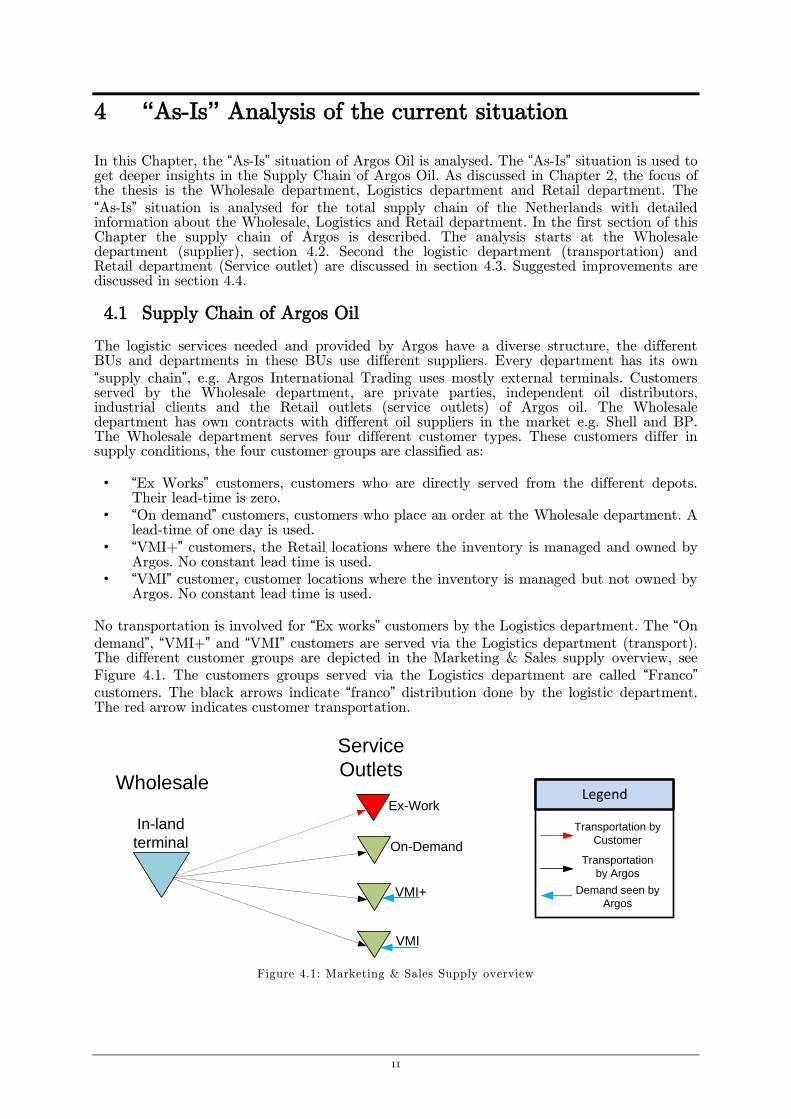
No transportation is involved for “Ex works” customers by the Logistics department. The “On
demand”, “VMI+” and “VMI” customers are served via the Logistics department (transport). The different customer groups are depicted in the Marketing & Sales supply overview, see
Figure 4.1. The customers groups served via the Logistics department are called “Franco”
customers. The black arrows indicate “franco” distribution done by the logistic department. The red arrow indicates customer transportation.
Figure 4.1: Marketing & Sales Supply overview
Wholesale
Service
Outlets
Ex-Work
On-Demand
VMI+
VMI
In-land
terminal
Legend
Transportation
by Argos
Transportation by
Customer
Demand seen by
Argos

4 “As-Is” Analysis of the current situation
12
The different terminals used by the Wholesale department are not owned by Argos. These terminals are operating with the use of a volume supply contract. When using a volume contract the supply, inventory and terminal are managed by an external party. In this concept a fixed volume per month is determined on a yearly basis. Argos commits to buy these volumes on yearly/monthly basis. The different terminals have different throughput
prices expressed in Euros per cubic meter, which are called in the oil industry “Ex. Rack”
prices. In this report “Ex. Rack” prices, depot costs and throughput costs are used interchangeable. The different departments and their processes are discussed in the next sections.
4.2 Wholesale supply strategy
The Wholesale department supplies gasoline, diesel and gasoil. Volume contracts are used for the majority of terminals. These volume contracts are signed on a yearly basis. To determine the needed volume the Wholesale department (contract owner) evaluates the demand of last year per terminal and increase or decrease this with a forecast factor. This aggregate yearly volume is divided by 12, to create a monthly demand. This monthly demand is used in the determination of the volume level for the volume contracts. The total amount of volume is
determined to cover the supply chain demand and “Ex Works” (B2B) demand. This is correct when there is no variation in demand. The contracts are almost fixed at the supply side and a variation in the loaded demand should almost be zero to avoid shortage or overshoot penalties in the end of the year. The supply side is completely committed (Argos buys a fixed volume per month) but the demand at the Wholesale department is however not fixed in volume. The Wholesale department has a no-commitment strategy based on a daily pricing strategy. The selling price of products is determined on a daily basis. Ex Works customers can load where they
want and how much they want on the total terminal network of Argos (in Dutch “vrijheid
blijheid”). The Logistics department is also free to load where they want in order to serve the (franco) customers. Free in this respect means that a depot is chosen from a number of depots that is appointed by the Wholesale department. This loading procedure occurs randomly at different depots and often leads to possible shortages or overshoots in oil products at several depots. At that moment (mostly at the end of the month) the Wholesale department anticipates for this unwanted effect and orders the logistic department which
depots to use to serve the “franco” customers. Figure 4.2 is used as an example to depict the effect of this anticipation with two terminals. In this example terminal 1 served to much customer demand and is almost facing an overshoot in depot capacity and terminal 2 served not enough demand and is almost facing an undershoot. The blue and green lines in Figure 4.2 depict the effect of the anticipation chosen by the Wholesale department.
Figure 4.2: Example of demand allocation change for two terminals
The need for anticipation is enlarged by the variation of the demand as depicted in Figure 4.3. The figure depicts the fluctuation of the supply chain demand in comparison with the average demand used in the determination of available volume at the depots. For example, in the months 1, 2, 7 and 8 the volume need for Gasoline and Diesel Oil is below average. When the demand/volume need is below average, the undershoot probability is higher for the
0 Time ->
Depot Capacity
0
Depot Capacity
Time ->
Anticipation, only Ex-works left
“Ex-Works” and “Franco”
Only “Ex Works”
Anticipation, all “Franco” demand
“Ex-Works” and “Franco”
“Ex-Works” and all
“Franco”
Terminal 1 Terminal 2
Contract volume
Contract volume

4 “As-Is” Analysis of the current situation
13
Wholesale department. In the months 3, 4, 6, 10, 11 and 12 the supply chain demand is above average and creates a higher probability of an overshoot. In the end, the supply chain
and “Ex Works” customers have to be served at all time. However, when changing the
allocation of the “franco” customers the Wholesale department is not able to observe the change in costs.
Figure 4.3: Comparison of Average “franco” demand vs. “franco” month demand
In addition to this anticipation (change of allocation) of the “franco” customers the price of
the oil product of each depot are changed differently in order to guide the “Ex Works” customers to particular (cheaper) depots. For example, the Wholesale department applies a higher price when there is a volume shortage and spot deals when there is an overshoot of volume at the end of the month.
By changing allocations of supply chain demand (“franco” customers) and at last the change
of pricing for “Ex Works” demand is used to cover the contracts. As discussed the Wholesale
department does not know the increase of cost when changing the allocation of the “franco” customers. Intuitively one should question if for example the increase (extra distance) of
transportation cost is less than a price decrease at the terminal with too much “open” demand (smaller profit). In the end all these costs are to be paid by Argos.
4.3 Logistics and Retail departments
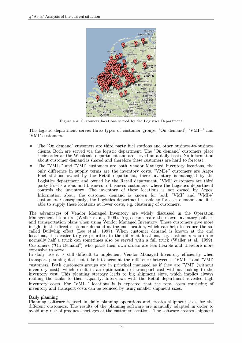
As discussed the Logistics department is responsible for the road transport of the different oil products sold by the Wholesale (franco delivered) and Retail department. This is the transport to the Wholesale customers and to the Retail fuel stations. The logistic department serves around 400 locations on yearly basis, as depicted in Figure 4.4.
4 “As-Is” Analysis of the current situation
14
Figure 4.4: Customers locations served by the Logistics Department
The logistic department serves three types of customer groups; “On demand”, “VMI+” and
“VMI” customers.
The “On demand” customers are third party fuel stations and other business-to-business
clients. Both are served via the logistic department. The “On demand” customers place their order at the Wholesale department and are served on a daily basis. No information about customer demand is shared and therefore these customers are hard to forecast.
The “VMI+” and “VMI” customers are both Vendor Managed Inventory locations, the
only difference in supply terms are the inventory costs. “VMI+” customers are Argos Fuel stations owned by the Retail department, there inventory is managed by the
Logistics department and owned by the Retail department. “VMI” customers are third party Fuel stations and business-to-business customers, where the Logistics department controls the inventory. The inventory of these locations is not owned by Argos.
Information about the customer demand is known for both “VMI” and “VMI+” customers. Consequently, the Logistics department is able to forecast demand and it is able to supply these locations at lower costs, e.g. clustering of customers.
The advantages of Vendor Managed Inventory are widely discussed in the Operation Management literature (Waller et al., 1999). Argos can create their own inventory policies and transportation plans when using Vendor Managed Inventory. These customers give more insight in the direct customer demand at the end location, which can help to reduce the so-called Bullwhip effect (Lee et.al., 1997). When customer demand is known at the end locations, it is easier to give priorities to the different locations, e.g. customers who order normally half a truck can sometimes also be served with a full truck (Waller et al., 1999).
Customers (“On Demand”) who place their own orders are less flexible and therefore more expensive to serve. In daily use it is still difficult to implement Vendor Managed Inventory efficiently when
transport planning does not take into account the difference between a “VMI+” and “VMI”
customers. Both customers groups are in principal managed as if they are “VMI” (without inventory cost), which result in an optimization of transport cost without looking to the inventory cost. This planning strategy leads to big shipment sizes, which implies always refilling the tanks to their capacity. Interviews with the Retail department revealed high
inventory costs. For “VMI+” locations it is expected that the total costs consisting of inventory and transport costs can be reduced by using smaller shipment sizes. Daily planning Planning software is used in daily planning operations and creates shipment sizes for the different customers. The results of the planning software are manually adapted in order to avoid any risk of product shortages at the customer locations. The software creates shipment
4 “As-Is” Analysis of the current situation
15
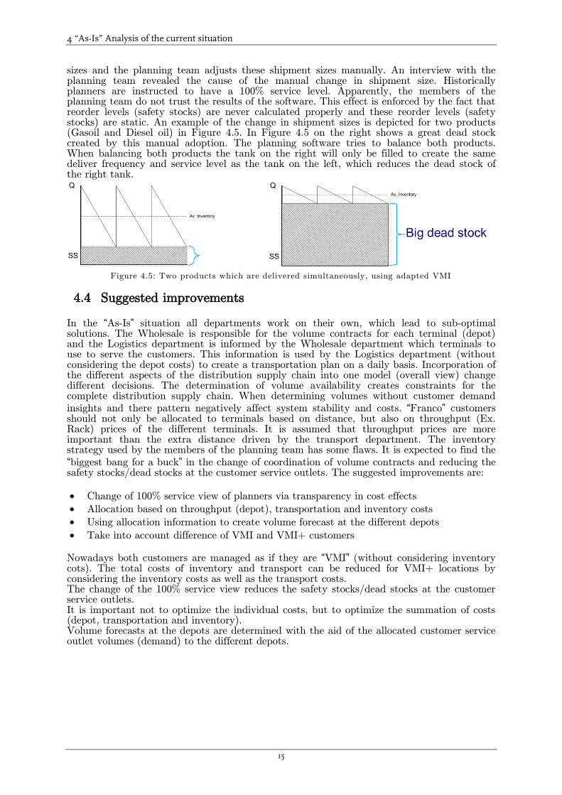
sizes and the planning team adjusts these shipment sizes manually. An interview with the planning team revealed the cause of the manual change in shipment size. Historically planners are instructed to have a 100% service level. Apparently, the members of the planning team do not trust the results of the software. This effect is enforced by the fact that reorder levels (safety stocks) are never calculated properly and these reorder levels (safety stocks) are static. An example of the change in shipment sizes is depicted for two products (Gasoil and Diesel oil) in Figure 4.5. In Figure 4.5 on the right shows a great dead stock created by this manual adoption. The planning software tries to balance both products. When balancing both products the tank on the right will only be filled to create the same deliver frequency and service level as the tank on the left, which reduces the dead stock of the right tank.
Figure 4.5: Two products which are delivered simultaneously, using adapted VMI
4.4 Suggested improvements
In the “As-Is” situation all departments work on their own, which lead to sub-optimal solutions. The Wholesale is responsible for the volume contracts for each terminal (depot) and the Logistics department is informed by the Wholesale department which terminals to use to serve the customers. This information is used by the Logistics department (without considering the depot costs) to create a transportation plan on a daily basis. Incorporation of the different aspects of the distribution supply chain into one model (overall view) change different decisions. The determination of volume availability creates constraints for the complete distribution supply chain. When determining volumes without customer demand
insights and there pattern negatively affect system stability and costs. “Franco” customers should not only be allocated to terminals based on distance, but also on throughput (Ex. Rack) prices of the different terminals. It is assumed that throughput prices are more important than the extra distance driven by the transport department. The inventory strategy used by the members of the planning team has some flaws. It is expected to find the
“biggest bang for a buck” in the change of coordination of volume contracts and reducing the safety stocks/dead stocks at the customer service outlets. The suggested improvements are:
Change of 100% service view of planners via transparency in cost effects
Allocation based on throughput (depot), transportation and inventory costs
Using allocation information to create volume forecast at the different depots
Take into account difference of VMI and VMI+ customers
Nowadays both customers are managed as if they are “VMI” (without considering inventory cots). The total costs of inventory and transport can be reduced for VMI+ locations by considering the inventory costs as well as the transport costs. The change of the 100% service view reduces the safety stocks/dead stocks at the customer service outlets. It is important not to optimize the individual costs, but to optimize the summation of costs (depot, transportation and inventory). Volume forecasts at the depots are determined with the aid of the allocated customer service outlet volumes (demand) to the different depots.

16
5 “To-Be” Design of suggested improvements
As stated in paragraph 4.1 the different departments are not connected with each other, each
department has its own “Supply Chain”. To conclude Argos has the components to create a complete integrated supply chain, but uses the different services independently for external customers. It is expected that the total relevant costs can be minimized by creating an integral distribution supply chain.
A “To-Be” design is created from the different department processes and product flows as
discussed in the “As-Is” situation. Starting from this “To-Be” design a model is created. With
the help of this model the “To-Be” concept is proven and the limitations of the model are discussed. With the results of this discussion a plan is created for the implementation at Argos. Furthermore the next steps for both scientific research and Argos are given.
5.1 Formulation of the “To Be” situation
As discussed in Chapter 2 this master thesis is focussed on the Logistics department and the connections with the Wholesale and Retail department. As discussed in Chapter 4 the volume determination of inland terminals (depots) is critical to manage business efficiently. Volumes for all terminals are fixed during the year and extra costs for covering these volumes (to prevent penalties) are minimized, e.g. allocation based on costs instead on volumes. The
design will focus on the allocation of the “franco” customers served by the logistic department. Volume contracts are determined with the use of a monthly forecasted allocation volume within the time span of a year. This procedure creates forecasted volumes for each terminal on a monthly basis. The year volume per terminal is the summation of the volumes determined per month. With this information volumes are better determined and the overall costs for Argos are minimized. The scope of the model is depicted in Figure 5.1. As discussed in Chapter 3 the created model should choose the optimal allocation (in terms of overall costs) and determine shipment sizes per customer per product. The model allocates more
than 380 “franco” customers to 14 different terminals.
Figure 5.1: Volume allocation problem of Argos
The “Ex Works” B2B customers are out of scope. The available customer data and the time
available for the thesis were not sufficient to incorporate the “Ex Works” customers. Consequently, their demand is determined independently of this model to create an overall forecast for the different terminals. The objective functions based on the scope are:
380+,
Service
Outlets
14, In-land
terminals
Legend
Terminal
Customer
Allocation linkChoice of allocation
Q Shipment size
Q

5 “To-Be” Design of suggested improvements
17
Depot costs
Road transport cost based on distance and shipment size
Inventory costs for Retail locations and safety stocks for Retail and Wholesale locations The model uses an integral cost function to create an overall Argos optimum solution. The model is further called integral model. The next section discusses the complex and dependent nature of the different parts of the cost function. Model decisions As discussed in the literature review designing a distribution supply chain in the oil and gas industry involves multiple decisions. These decisions are classified by Facility location decisions, transportation decisions and inventory decisions. Argos Oil is a constant growing player in the downstream part of the oil and gas industry. As a result there is a need for a complete design of the supply chain of Argos Oil for multiple products. The different decisions needed to make are depicted in Table 5.1. The input parameters for the model are represented in red and the optimization variables of the model are depicted in grey.
Table 5.1: Integral model decisions
5.2 Cost functions Argos Oil
To get deeper into the problem the different cost functions faced by the distribution supply chain of Argos are discussed. These cost functions are explained and integrated into one function used by the Integral model. Depot cost The depot cost, valid for terminals with a volume contract, are calculated based on a fixed
volume price. The fixed volume price is called “throughput cost” in the model. In this way the equation for each shipment size is derived.
33(1)
€Depot cost € = Fixed Ex-rack (throughput) cost Shipmentsize (5.1)volume mm
In the developed integral model the depot costs are based on a volume contract. This is done, because the majority of terminals used have a volume contract. Argos does not own an inland terminal with facilities to serve trucks (road transport). The equation (5.1) is converted to a function (5.2) that is valid to calculate the depot costs on a monthly basis:
3
3€ €Depot cost = Demand Throughput cost
month monthmonth monthm
m
(5.2)
For each terminal a throughput cost is determined in this way. Throughput cost varies between the different terminals. The terminals which are deeper located in the hinterland
Logistics
DecisionsInland Terminal Location Transportation Inventory
Number of Terminals Mode Supplier selection
Location of Terminals Type of carriage Total system volume
Assignment of Terminals to supply sources Location of available volume
Allocation of demand to Terminals
Shipment volume Size of inventories at various locations
Levels of safety stock at various locations
Control discipline at various locations
Strategic
Tactical
Operational
Integral model

5 “To-Be” Design of suggested improvements
18
generate higher inbound transportation costs, based on distance and possible the use of smaller barges. Furthermore, the different terminal owners have their own cost strategy that also affects the throughput cost for each terminal. In the integral model the total costs are minimized. Therefore it is expected that the majority of the demand will be directed to cheaper depots (terminals) in terms of throughput costs. Remark: The fixed costs to open and use a terminal are not included in the integral model as a separate cost. It should be mentioned that the used solver (OpenSolver) in excel is not able to find an optimal solution when incorporating opening and closing decisions. This problem can be solved by using heuristics or another solver, e.g. CPLEX. In the integral model opening and closing decisions can be made manually by the user. A side effect of closing and opening a terminal will have a direct impact on the service seen by the Wholesale customers
“Ex Works”. Closing and opening should therefore not only be based on the “franco” customers, which are in scope. Transport costs The transport cost function is based on the remarks of Daganzo (2005), using variable cost for the distance and variable cost for the (un)loading time, see Chapter 3.2. The cost function is divided into two parts related to the distance costs and waiting time costs. The costs related to the distance (dis) depends on the distance cost per kilometre (kc) and the time dependent distance cost. The latter is calculated via the time cost (tc) divided by the average speed of the truck (asp). The costs related to the waiting time depends on a fixed part and a variable part. The fixed part is related to the queue time at the depot (dt) and the login time at the customer (ct). The variable part consists of the loading time (lt) and unloading time (ut) both multiplied with the shipment size (Q). The following expression (5.3) for the direct transport cost function is in this way derived.
(5.3)+ + tc
dis kc tc dt lt ut Q ctasp
In reality a truck follows a route and visits various customers. A simple adoption is used to approximate the route transportation costs. For that reason the costs related to the queue time at the depot are equally divided by the shipment sizes of the customers. This is done by replacing queue time (dt) by a linear function of the shipment size (Q), Z*Q. The factor Z is a simple cost allocation factor which depends either on the maximum truck volume (ttv) or maximum truck load (ttw). The following expression for the cost allocation factor Z is derived:
if
otherwise
dt Q Q
ttw ttw ttvZ
dt
ttv
In which the density ρ of the product is used to determine the shipment weight. Effects of other products (different customers) in the truck are not incorporated in the cost function. Another adjustment is necessary to approximate the route transportation costs, depicted in Figure 3.1. The adjustment done is on a general level. The distance of the direct transportation is multiplied by a correction factor p. However, this is not exact because this correction factor is likely to be depended on the shipment size. The creation of a more exact equation is complicated in an allocation model, it is not known on forehand, which customers can be clustered and is therefore left out of scope. The function with these two adaptions is depicted in expression (5.4).
+ + (5.4)ij ij i j ij j
tcp dis kc tc Z Q lt ut Q ct
asp
5 “To-Be” Design of suggested improvements
19
The following assumptions are used in expression (5.4):
Truck always leaves the depot i completely full, truck can serve multiple customers thereby shares the fixed waiting time at depot i (dti)
The distance costs are based on direct transportation
The average speed (asp) is constant for every route
(un)loading times are linear (lti, utj)
Z factor is only correct if the different are slightly different
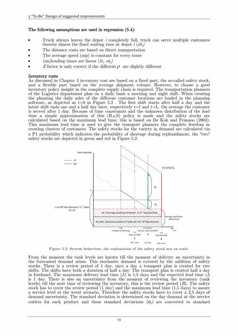
Inventory costs As discussed in Chapter 3 inventory cost are based on a fixed part, the so-called safety stock, and a flexible part based on the average shipment volume. However, to choose a good inventory policy insight in the complete supply chain is required. The transportation planners of the Logistics department plan on a daily basis a morning and night shift. When creating the planning the daily sales of the different customer locations are loaded in the planning software, as depicted as t=0 in Figure 5.2 . The first shift starts after half a day and the latest shift ends one and a half day later, respectively t=l and t=L. On average the customer is served after 1 day. Because of time constraints and the unknown distribution of the lead time a simple approximation of this (R,s,S) policy is made and the safety stocks are calculated based on the maximum lead time, this is based on De Kok and Fransoo (2003). This maximum lead time is used to give the transport planners the complete freedom in creating clusters of customers. The safety stocks for the variety in demand are calculated via
a P1 probability which indicates the probability of shortage during replenishment, the “two” safety stocks are depicted in green and red in Figure 5.2.
Figure 5.2: System behaviour, the explanation of the safety stock not on scale.
From the moment the tank levels are known till the moment of delivery an uncertainty in the forecasted demand arises. This stochastic demand is covered by the addition of safety stocks. There is a review period of 1 day, once a day a transport plan is created for two shifts. The shifts have both a duration of half a day. The transport plan is created half a day in forehand. The maximum delivery lead time (L) is 1,5 days and the expected lead time (l) is 1 day. There is also an uncertainty from the moment of reviewing the inventory (tank levels) till the next time of reviewing the inventory, this is the review period (R). The safety stock has to cover the review period (1 day) and the maximum lead time (1,5 days) to assure a service level at the worst scenario. Therefore the safety stocks have to cover a 2,5 days of demand uncertainty. The standard deviation is determined on the day demand at the service
outlets for each product and these standard deviations (σf) are converted to standard
Time
Av.Q=Qf+Qv
t=0 Creation of Planning
t=l Start 1st Shift
t=(L-l)/2+lEnd 1st, start 2nd Shift
t=LEnd 2nd Shift
SS_Max. Demand variation=k*stdev of L+R + R*Day Demand
Av. Coverage planning variation= (L-l) * Day Demand
Qf
Qv
s
Min. Time Av. Time Max. Time
Tank volume
Average Dead Stock, Safety Stock
s =(L+R)*Day Demand + k * stdev of L+R
IP
OH

5 “To-Be” Design of suggested improvements
20
deviations (σL+R) during the lead time and review period of in total 2,5 days. The demand pattern is analyzed with @Risk and a normal distribution is found to be applicable on almost all customer locations. Also the coefficient of variation (C.V) that is the standard deviation
σL+R over the average demand hL+R is smaller than 0,5. (Silver et.al. 1998) The coefficient of variation was on average bellow 0,3 which is much smaller than the maximum of 0,5. The demand distribution is assumed to be normal distributed for all locations. Therefore the following formula (5.5) can be applied to calculate the standard deviation of a different time period of 2,5 days.
* 2,5 * (5.5)L R f fL R
Table 5.2: Safety stock variables
Variable Definition
L R Standard deviation of error forecasted demand, during lead-time L and review
period R
f Standard deviation of error forecasted demand for one day
The trigger level s is determined without considering the undershoot of the demand through the trigger level. The expected undershoot changes with the shipment size (tank size) and cannot easily be incorporated in a linear model.
Figure 5.3: Safety Stock explanation
For safety reasons the trigger level is the demand during the review period and the maximum lead time and uncertainty in forecasted demand, as depicted in equation (5.6). The standing still stock (Safety Stock) is the demand during the maximum lead time and review period minus the expected lead time demand plus the stock for covering uncertainties in the demand pattern, depicted in equation (5.7)
[ ] (5.6)L R L R us E h k x [ ] (5.7)L R l L R uSS E h h k x
The safety stock (SS) is used in the shipment size determination in the integral model. The shipment size has multiple constraints and the tank availability is determined with the help of the safety stock as depicted in function (5.8). The Q is the average maximum shipment size used in the integral model and the free tank capacity is determined by the tank capacity3 multiplied with the usable space factor (T) minus the average standing still stock (SS), see equation (5.8). Note that in daily use tank availability changes with the time of arrival chosen by the daily planning system.
Tankcapacity (5.8)Q T SS
3 Summation of the individual tanks capacities at the customer service outlet per product type
P1=98% k= 2,05

5 “To-Be” Design of suggested improvements
21
Safety stocks are calculated via a specified probability (P1) which indicates the so called Cycle service level. The specified probability (P1) is the probability of no stock out during the replenishment cycle (de Kok, 2005). A specified fraction (P2) is the fill-rate and is the demand to be satisfied routinely from the tank. For linearity reasons and contracts at Argos a specified probability (P1) is chosen, for a specified fraction (P2) the shipment size is needed and this makes the optimization problem non-linear. The specified probability (P1) is a safe measure and assures a minimum safety level equal or greater than a specified fraction (P2). The difference of P1 and P2 is that the P1 only takes into account the replenishment cycle and P2 takes into account the probability of the demand to be satisfied routinely from the customer service outlet. Both the use of a specified fraction (P2) and the incorporation of undershoots will reduce safety stocks and are important for further expansions. Finally, the inventory costs in the model are approximated via equation 5.9. The different notations are explained in Table 5.3.
.
Inv. Cost [€]= [ ] (5.9)2
L R l L R u
Av QE h h k x v r
Table 5.3: Variables for the Inventory cost function
Notation Definition
Av.Q Average shipment size [m3]
Qf Fixed part of average shipment size [m3]
Qv Variable part of average shipment size [m3]
hL,j The average demand during lead-time (L) [m3]
hl,j The average demand during the replenishment-time (l) [m3]
k Service level factor
L+R The standard deviation of the demand during the lead-time (L+R)
v The price of one unit [€/unit]
r The interest rate for holding stock [%]
xu Unusable stock in tank [m3]
The inventory cost function (5.5) is based on a fixed part the so-called safety stock and a flexible part based on the average shipment volume. The fixed part is the average extra stock (E[hL+R-hl]) to cover the possibility of clustering orders (choice first shift or second shift), the
safety stock to cover the demand variability during the lead-time (L+R) with a service measure (k) and the unusable stock in a tank (xu). The variable part is based on the average shipment size (Av.Q) divided by 2. Both the fixed and variable part are multiplied with the costs of holding stock (v*r). The average shipment size is based on a fixed part (Qf) and a variable part (Qv). The variable part is on average half of the demand during the lead time of two shifts ((L-l)/2) and the extra stock needed (E[hR]) for the possible undershoot of the replenishment level (s). The possibility of undershoot is not incorporated in the integral model. This and the variable lead time can be included by an extended version of the model. However, including these aspects now does not make any sense when forecasts are not created. The used standard deviations are not accurately enough to adapt the model. Also the distribution of the lead time of the two shifts is unknown, approaching it with a normal distribution will only create more safety stock on high service levels.
5.3 Integral model creation
The integral model is created from a Single Echelon Single Commodity location model (Ghiani et. Al, 2004), the option to open/close a facility is withdrawn from the minimization function, which creates a single commodity allocation model. The original model uses a unit
price per item [€/unit] to allocate units of demand. This is changed to a different cost function that includes a direct transportation cost and inventory costs, which changes with the shipment size. This results in a function with two variables, respectively allocation of demand and shipment size choice. The created model assumes indivisible demand. The allocation of customer demand cannot be divided to more than one supplier location. This could however affect the optimal solution of
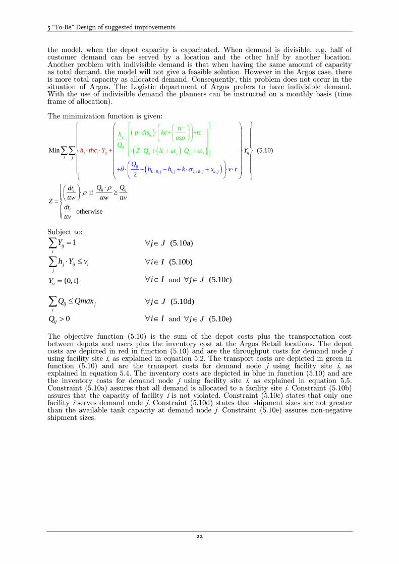
5 “To-Be” Design of suggested improvements
22
the model, when the depot capacity is capacitated. When demand is divisible, e.g. half of customer demand can be served by a location and the other half by another location. Another problem with indivisible demand is that when having the same amount of capacity as total demand, the model will not give a feasible solution. However in the Argos case, there is more total capacity as allocated demand. Consequently, this problem does not occur in the situation of Argos. The Logistic department of Argos prefers to have indivisible demand. With the use of indivisible demand the planners can be instructed on a monthly basis (time frame of allocation). The minimization function is given:
, , , ,
Min (5.1
+
0
2
)
+
i
ijj
ij
ij i ij
i j
j
L R j l j L
j ij jj i i
R
j
j u j
tcp dis
Y
kc tchasp
QZ Q
Qh h
lt u
k x v r
t Q cth thc Y
if
otherwise
ij iji
i
Q Qdt
ttw ttw ttvZ
dt
ttv
Subject to:
1ij
i
Y (5.10a)j J
j ij i
j
h Y v (5.10b)i I
{0,1}ijY
i I and (5.10c)j J
ij j
i
Q Qmax (5.10d)j J
0ijQ
i I and (5.10e)j J The objective function (5.10) is the sum of the depot costs plus the transportation cost between depots and users plus the inventory cost at the Argos Retail locations. The depot costs are depicted in red in function (5.10) and are the throughput costs for demand node j using facility site i, as explained in equation 5.2. The transport costs are depicted in green in function (5.10) and are the transport costs for demand node j using facility site i, as explained in equation 5.4. The inventory costs are depicted in blue in function (5.10) and are the inventory costs for demand node j using facility site i, as explained in equation 5.5. Constraint (5.10a) assures that all demand is allocated to a facility site i. Constraint (5.10b) assures that the capacity of facility i is not violated. Constraint (5.10c) states that only one facility i serves demand node j. Constraint (5.10d) states that shipment sizes are not greater than the available tank capacity at demand node j. Constraint (5.10e) assures non-negative shipment sizes.

5 “To-Be” Design of suggested improvements
23
Table 5.4: Variables and notations used in the Integral model
Notation Definition I Set of facility sites J Set of demand nodes hj demand at node j [unit(s)] thci Throughput cost depot i for product 1 vi Volume available at facility site i hj Month forecasted demand of node j [unit(s)] Qij Shipment size from depot i to node j [unit(s)] Qmaxij Maximum Shipment size from depot i to node j [unit(s)], constrained by Tank
size of service outlet and maximum truck volume kc Price per travelled km [€/km] asp Kilometre per hour [km/hour]
tc Price per time [€/hour] dtj Waiting time at depot j [hour] ttv The maximum truck volume (capacity) [m3] ltj The loading time/pumpspeed-1 [hour/m3] uti The unloading time/pumpspeed-1 [hour/m3] cti Waiting time at Retailer/customer i [hour] hL,j The average demand during lead-time (L) for node j [unit(s)] k Service level factor
L+R,j The standard deviation of the demand during the lead time and replenishment of node j
v The price of one unit [€/unit] r The interest rate for holding stock [%] p Scale factor, change transportation cost by changing relative distance [%] hl,j The average demand during the replenishment-time (l) for node j [unit(s)] Z Cost allocation factor for the Depot waiting time dti [hours]
Binary, choice of having inventory cost {0,1}
Decision variables Definition Yij 1 if demand at node j is served by facility at node i 0 if not Qij Shipment size from depot i to node j [unit(s)]
The model proposed in function (5.10) is non-linear, e.g. the shipment size (Qij) influences the inventory costs and the transportation costs. The shipment size (Qij) can take all values and is multiplied with a binary variable (Yij) this results in a Mixed Integer Non-linear problem (MINLP). The Integral model is a MINLP, which is hard to solve in standard (free) solvers. The company prefers the use of the program Excel and therefore the MINLP problem is decomposed to two modules to be able to solve the problem in Excel. The problem will be solved in excel with the use of Opensolver®. The Integral model has two variables which have to be optimized i.e. shipment sizes and allocations, see Figure 5.4. The Integral model is expanded to three commodities and the possibility of combined shipping. With the use of combined shipping the real costs are better approximated and the model will therefore favour a location where multiple products can be loaded. Section 5.5 presents a module to create the optimal shipment sizes for every possible allocation. These shipments sizes create different cost matrices, called cij. These cost matrices are the input for the allocation model described in section 5.6.

5 “To-Be” Design of suggested improvements
24
Figure 5.4, Conversion of Integral model to sub-models
5.4 Module 1: Shipment size determination model
As discussed the Integral model is decomposed to two modules. The problem can be solved in Excel via these two modules. For the users it is also easier to add constraints and change cost functions in both modules. To be able to solve the Integral model first the different optimal shipment sizes are calculated for every possible link in module 1. This solved by minimizing the summation of transport and inventory costs. The different shipment sizes are used to create cost matrices, as depicted in Figure 5.5. With the use of this information module 2 only needs to select the cheapest allocation taken into account depot costs and depot capacities. First, in module 1 for every combination the shipment size needs to be determined.
Figure 5.5: Module 1, Shipment size determination tool
Two types of cost functions namely, a single product and a combined shipping of two products at once, are used in module 1. First the single product transportation and inventory cost function is explained which is applied for the products Gasoline, Diesel and Gasoil, respectively product 1,2 and 3. The single product cost function is given in equation (5.11) and is a combination of the functions given in (5.4) and (5.9).
, , , ,
The generated Cost to serve a customer service outlet from depot is represented by (C )
+ +
2
ij
ijj ij
L R j l j L R j u j
ij
ij i j ij j
j i
tcp dis kc tch Q
asp h h k xQ
Z Q lt ut Q ct
(5.11)monthv r
Integral model
Optimizes:- Allocation- Shipment size
Module 1: Shipment size determination tool
Optimizes:- Multiple product shipment sizes for all possible allocations
Module 2: Allocation tool
Optimizes:- Allocation to different terminals
Output: Transport + Inventory cost matrices (Cij)
Output: Allocation choices with shipment sizes and costs
Module 1: Shipment size determination tool
Optimizes:- Multiple product shipment sizes for all possible allocations
Output: Transport + Inventory cost matrices (Cij)
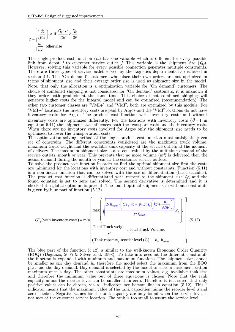
5 “To-Be” Design of suggested improvements
25
if
otherwise
ij iji
i
Q Qdt
ttw ttw ttvZ
dt
ttv
The single product cost function (cij) has one variable which is different for every possible link from depot i to customer service outlet j. This variable is the shipment size (Qij). However, solving this variable for every possible connection generates multiple constraints. There are three types of service outlet served by the Logistics departments as discussed in
section 4.1. The “On demand” customers who place their own orders are not optimized in terms of shipment size and their average order size is used as shipment size in the model.
Note, that only the allocation is a optimization variable for “On demand” customers. The
choice of combined shipping is not considered for “On demand” customers, it is unknown if they order both products at the same time. This choice of not combined shipping will generate higher costs for the Integral model and can be optimized (recommendation). The
other two customer classes are “VMI+” and “VMI”, both are optimized by this module. For
“VMI+” locations the inventory costs are paid by Argos and the “VMI” locations do not have inventory costs for Argos. The product cost function with inventory costs and without
inventory costs are optimized differently. For the locations with inventory costs ( =1 in equation 5.11) the shipment size influences both the transport costs and the inventory costs. When there are no inventory costs involved for Argos only the shipment size needs to be optimized to lower the transportation costs. The optimization solving method of the single product cost function must satisfy the given set of constrains. The different constraints considered are the maximum truck volume, maximum truck weight and the available tank capacity at the service outlets at the moment of delivery. The maximum shipment size is also constrained by the unit time demand of the service outlets, month or year. This prevents that no more volume (m3) is delivered then the actual demand during the month or year at the customer service outlets. To solve the product cost function in order to find the optimal shipment size first the costs are minimized for the locations with inventory cost and without constraints. Function (5.11) is a non-lineair function that can be solved with the use of differentiation (basic calculus). The product cost function is differentiated with respect to the shipment size Qij and the found equation is set to zero and solved. The second derivative is determined and it is checked if a global optimum is present. The found optimal shipment size without constraints is given by blue part of function (5.12).
*
max , ,
(with inventory costs) min
Total Truck weight, Total Truck Volume,
Tank capacity -reorder level (s) ,
2 month j ij
mo
l
ij
i l mon
n h
th
t
tch CT tc p Dis kc
ASP
rh
Q
h h
v
(5.12)
The blue part of the function (5.12) is similar to the well-known Economic Order Quantity (EOQ) (Daganzo, 2005 & Silver et.al. 1998). To take into account the different constraints the function is expanded with minimum and maximum functions. The shipment size cannot be smaller as one day demand hl, therefore the model select the maximum from the EOQ part and the day demand. Day demand is selected by the model to serve a customer location maximum once a day. The other constraints are maximum values, e.g. available tank size and therefore the minimum value out of three equations is chosen. Note that the tank capacity minus the reorder level can be smaller than zero. Therefore it is assured that only positive values can be chosen, via a +
indicator, see bottom line in equation (5.12). This + indicator means that the maximum value of the tank capacities minus the reorder level s and zero is taken. Negative values for the tank capacity are only found when the service level is not met at the customer service location. The tank is too small to assure the service level.
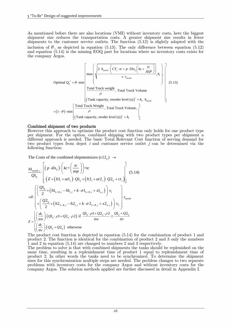
5 “To-Be” Design of suggested improvements
26
As mentioned before there are also locations (VMI) without inventory costs, here the biggest shipment size reduces the transportation costs. A greater shipment size results in fewer shipments to the customer service outlets. The function (5.12) is slightly adapted with the
inclusion of , as depicted in equation (5.13). The only difference between equation (5.12) and equation (5.14) is the missing EOQ part for locations where no inventory costs exists for the company Argos.
*
2
max , ,
Optimal min
Total Truck weight, Total Truck Volume
Tank capacity -reorder level (s) ,
month j ij
l
month
ij
i l month
tch CT tc p Dis kc
ASPh
v r
Q
h h
(5.13)
Total Truck Weight, Total Truck Volume,
1 min
Tank capacity -reoder level (s)i lh
Combined shipment of two products However this approach to optimize the product cost function only holds for one product type per shipment. For the option, combined shipping with two product types per shipment a different approach is needed. The basic Total Relevant Cost function of serving demand for two product types from depot i and customer service outlet j can be determined via the following function:
,
, , , , 1
The Costs of the combined shipmentsizes (c12 )
+ +1 (5.14)
11 1 1 2 2 2
11 1 1 1
2
2
ij
ijmonth j
ij
i j ij i j ij j
ij
L R j l j L R j u j
tcp dis kc tch
aspQ
Z lt ut Q lt ut Q ct
Qh h k x v
Q
, , , , 22 2 2 22
month
ij
L R j l j L R j u j
r
h h k x v
1 1 2 2 1 21 1 2 2 if
1 2 otherwise
ij ij ij ijiij ij
iij ij
Q Q Q QdtQ Q
ttw ttw ttvZ
dtQ Q
ttv
The product cost function is depicted in equation (5.14) for the combination of product 1 and product 2. The function is identical for the combination of product 2 and 3 only the numbers 1 and 2 in equation (5.14) are changed to numbers 2 and 3 respectively. The problem to solve is that with combined shipments the tanks should be replenished on the same time, resulting in a replenishment time of product 1 equal to replenishment time of product 2. In other words the tanks need to be synchronized. To determine the shipment sizes for this synchronization multiple steps are needed. The problem changes to two separate problems with inventory costs for the company Argos and without inventory costs for the company Argos. The solution methods applied are further discussed in detail in Appendix I.

5 “To-Be” Design of suggested improvements
27
The following assumptions are made for the Cost functions that depend of the shipment sizes:
A truck always leaves the depot i completely full and the truck can serve multiple customers and thereby shares the fixed waiting time at depot i (dti)
The distance costs are based on direct transportation
The average truck speed (asp) is constant for every route
(un)loading times are linear (lti, utj)
Inventory costs are linear
The ordering cost is constant for a possible connection from the depot i to customer service outlet j, because direct transportation is applied.
The rate of demand is constant
The lead time is fixed
The purchase price of the item is constant i.e. no discount is available
The replenishment is made instantaneously, the whole batch is delivered at once.
Interest rate is equal for all products, the company uses one interest rate.
Remarks: The distance of the direct transportation is multiplied with a correction factor p to approximate the actual route distance. The average truck speed is not in all areas in The Netherlands constant. It is lower in the cities compared to the average speed in rural areas. Also the time of the day affects the average speed. This average truck speed is based on the use of a morning and night shift respectively with lower and higher average truck speeds. The (expected) lead time is fixed on one day to calculate the average shipment size. In reality the delivery lead time varies between 0,5 and 1,5 days and thus an average value is chosen. Shipment sizes vary with the delivery lead time, as depicted (Qv) in Figure 5.2. Conclusion Module 1 optimizes shipment sizes for all locations and shipment possibilities as combined shipping or single product shipping. The module has different matrices as an output, c1ij, c2ij, c3ij, for the transportation and inventory costs of product 1,2 and 3 respectively. It also provides the cost matrices c12ij, c23ij for the transportation and inventory costs of combined shipping of product 1 and 2 and product 2 and product 3 respectively.
5.5 Module 2: Allocation model
What every allocation decision cost with respect to transportation and inventory is determined in module 1 and these results are laid down in different cost matrices. To solve the optimal allocation for all customers and to choose between combined product shipping transport and single product type transport a model is developed. The discussed model is an allocation model that is called module 2.
Figure 5.6: Module 2, Allocation tool
The model minimizes the overall costs by allocating the different end locations j per product type to the different depots i. The allocation is constrained by the different volumes available
Module 2: Allocation tool
Optimizes:- Allocation to different terminals
Output: Allocation choices with shipment sizes and costs
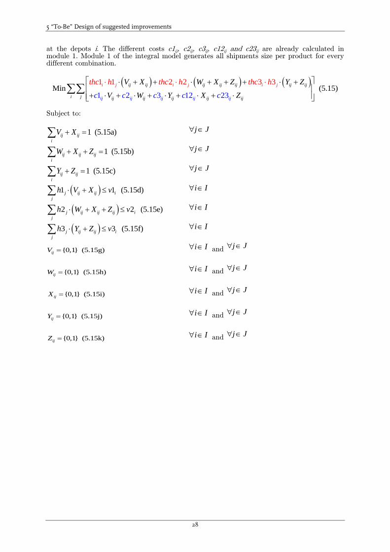
5 “To-Be” Design of suggested improvements
28
at the depots i. The different costs c1ij, c2ij, c3ij, c12ij and c23ij are already calculated in module 1. Module 1 of the integral model generates all shipments size per product for every different combination.
Min
1 2 3 12 2 (5.15)
1 1 2
3
2 3 3
i
ij ij ij ij ij ij ij
i j ij ij ij ij ij ij ij
i j i j i
i
j
jj ij
V Xthc h thc h thc hW X Z Y Z
V W Y Xc c Zc c c
Subject to:
1 (5.15a)ij ij
i
V X j J
1 (5.15b)ij ij ij
i
W X Z j J
1 (5.15c)ij ij
i
Y Z j J
1 1 (5.15d)j ij ij i
j
h V X v i I
2 2 (5.15e)j ij ij ij i
j
h W X Z v i I
3 3 (5.15f)j ij ij i
j
h Y Z v i I
{0,1} (5.15g)ijV i I and j J
{0,1} (5.15h)ijW i I and j J
{0,1} (5.15i)ijX i I and j J
{0,1} (5.15j)ijY i I and j J
{0,1} (5.15k)ijZ i I and j J
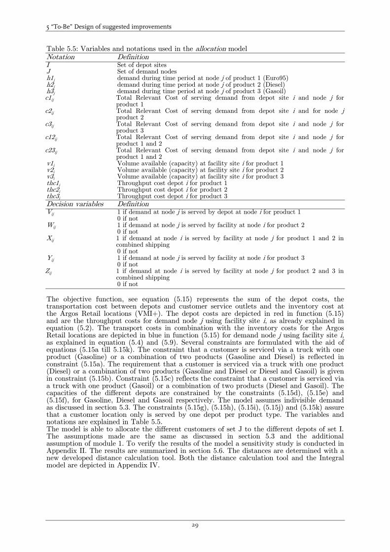
5 “To-Be” Design of suggested improvements
29
Table 5.5: Variables and notations used in the allocation model
Notation Definition I Set of depot sites J Set of demand nodes h1j demand during time period at node j of product 1 (Euro95) h2j demand during time period at node j of product 2 (Diesel) h3j demand during time period at node j of product 3 (Gasoil) c1ij Total Relevant Cost of serving demand from depot site i and node j for
product 1 c2ij Total Relevant Cost of serving demand from depot site i and for node j
product 2 c3ij Total Relevant Cost of serving demand from depot site i and node j for
product 3 c12ij Total Relevant Cost of serving demand from depot site i and node j for
product 1 and 2 c23ij Total Relevant Cost of serving demand from depot site i and node j for
product 1 and 2 v1i Volume available (capacity) at facility site i for product 1 v2i Volume available (capacity) at facility site i for product 2 v3i Volume available (capacity) at facility site i for product 3 thc1i Throughput cost depot i for product 1 thc2i Throughput cost depot i for product 2 thc3i Throughput cost depot i for product 3
Decision variables Definition Vij 1 if demand at node j is served by depot at node i for product 1 0 if not Wij 1 if demand at node j is served by facility at node i for product 2 0 if not Xij 1 if demand at node i is served by facility at node j for product 1 and 2 in
combined shipping 0 if not Yij 1 if demand at node j is served by facility at node i for product 3 0 if not Zij 1 if demand at node i is served by facility at node j for product 2 and 3 in
combined shipping 0 if not
The objective function, see equation (5.15) represents the sum of the depot costs, the transportation cost between depots and customer service outlets and the inventory cost at the Argos Retail locations (VMI+). The depot costs are depicted in red in function (5.15) and are the throughput costs for demand node j using facility site i, as already explained in equation (5.2). The transport costs in combination with the inventory costs for the Argos Retail locations are depicted in blue in function (5.15) for demand node j using facility site i, as explained in equation (5.4) and (5.9). Several constraints are formulated with the aid of equations (5.15a till 5.15k). The constraint that a customer is serviced via a truck with one product (Gasoline) or a combination of two products (Gasoline and Diesel) is reflected in constraint (5.15a). The requirement that a customer is serviced via a truck with one product (Diesel) or a combination of two products (Gasoline and Diesel or Diesel and Gasoil) is given in constraint (5.15b). Constraint (5.15c) reflects the constraint that a customer is serviced via a truck with one product (Gasoil) or a combination of two products (Diesel and Gasoil). The capacities of the different depots are constrained by the constraints (5.15d), (5.15e) and (5.15f), for Gasoline, Diesel and Gasoil respectively. The model assumes indivisible demand as discussed in section 5.3. The constraints (5.15g), (5.15h), (5.15i), (5.15j) and (5.15k) assure that a customer location only is served by one depot per product type. The variables and notations are explained in Table 5.5. The model is able to allocate the different customers of set J to the different depots of set I. The assumptions made are the same as discussed in section 5.3 and the additional assumption of module 1. To verify the results of the model a sensitivity study is conducted in Appendix II. The results are summarized in section 5.6. The distances are determined with a new developed distance calculation tool. Both the distance calculation tool and the Integral model are depicted in Appendix IV.
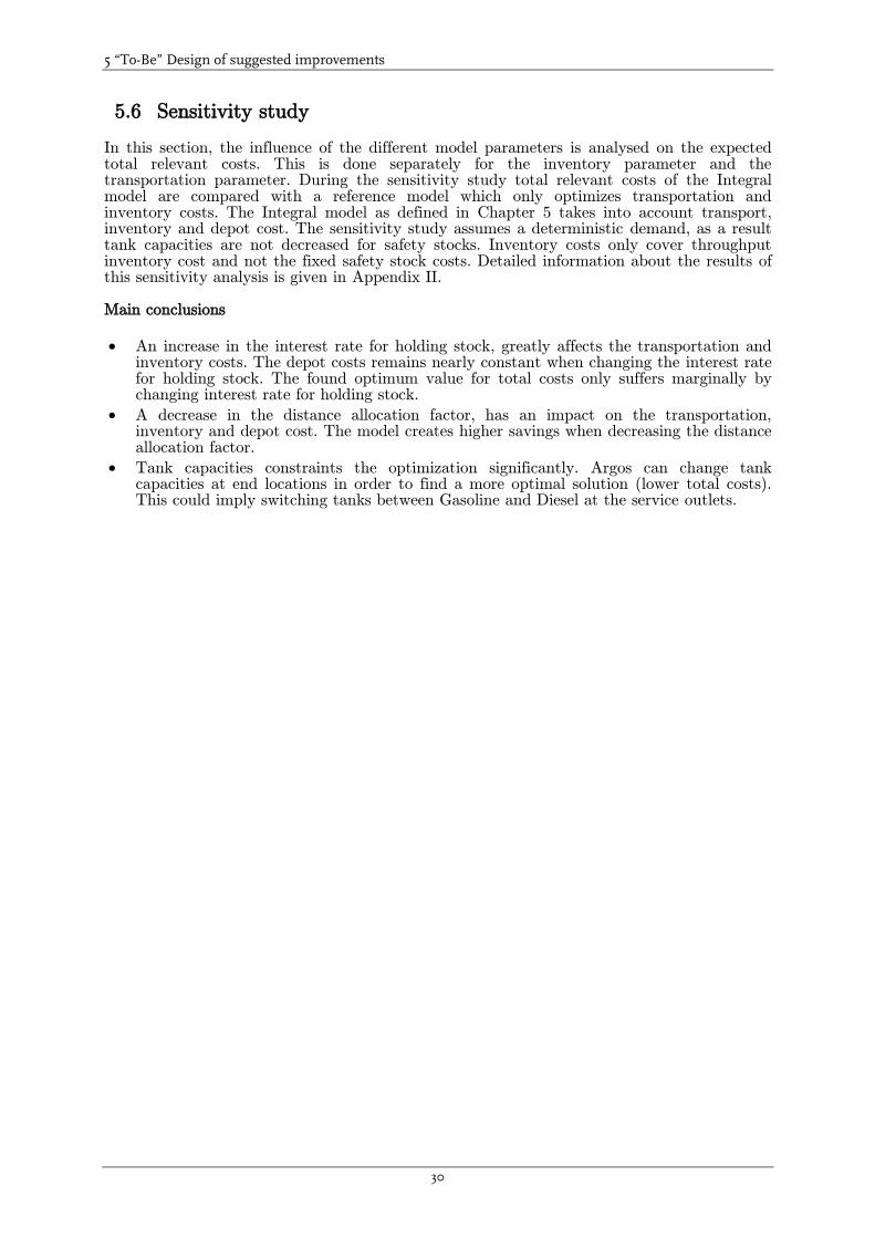
5 “To-Be” Design of suggested improvements
30
5.6 Sensitivity study
In this section, the influence of the different model parameters is analysed on the expected total relevant costs. This is done separately for the inventory parameter and the transportation parameter. During the sensitivity study total relevant costs of the Integral model are compared with a reference model which only optimizes transportation and inventory costs. The Integral model as defined in Chapter 5 takes into account transport, inventory and depot cost. The sensitivity study assumes a deterministic demand, as a result tank capacities are not decreased for safety stocks. Inventory costs only cover throughput inventory cost and not the fixed safety stock costs. Detailed information about the results of this sensitivity analysis is given in Appendix II. Main conclusions
An increase in the interest rate for holding stock, greatly affects the transportation and inventory costs. The depot costs remains nearly constant when changing the interest rate for holding stock. The found optimum value for total costs only suffers marginally by changing interest rate for holding stock.
A decrease in the distance allocation factor, has an impact on the transportation, inventory and depot cost. The model creates higher savings when decreasing the distance allocation factor.
Tank capacities constraints the optimization significantly. Argos can change tank capacities at end locations in order to find a more optimal solution (lower total costs). This could imply switching tanks between Gasoline and Diesel at the service outlets.

31
6 Analysis of cost savings in “To-Be” situation
In this Chapter the various costs, namely transportation, inventory, depot and total costs are
determined. First the costs in the “As-Is” situation are calculated. Second in section 6.2, with the developed Integral model and a basic set of parameters, a first optimization of the various
costs in the “As-Is” situation is determined. In section 6.3 an optimization of the “As-Is” situation is carried out. The depot costs, service levels, distance cost allocation factor and the capacities of the different tanks at the customer service outlets are varied. The effect on the optimization of different depot throughput prices is studied. Starting point in these optimizations are the loaded and verified volumes in the month December. In section 6.4 seven different What If scenarios are analysed to find how the different costs are affected. Finally, in section 6.5, the loaded volumes are estimated on a yearly basis. The effect of different parameters on the optimal cost values is studied for the complete year.
6.1 Baseline: “As-Is” of the Month December
In order to describe the “As-Is” situation all orders in the month December are analysed. The
demand per product and the loading location (depot) are used to determine the “As-Is” costs.
The “As-Is” comprises transport costs, depot costs and inventory costs and the determination of these costs are described in detail. For every order the transport costs are calculated via equation 6.1. The function is an adapted version of formula (5.4) used in the Integral model. This function calculates the costs for three products namely Gasoline, Diesel and Gasoil at once. The Integral model uses separate cost functions for each product or uses a different cost function for a combination of two products. These cost functions are described in detail in Chapter 5. A distance allocation factor p of 0,9 and an average speed asp of 60km/h are used. The different applied costs parameters and time parameters are depicted in appendix III.
1 2 3 1 1 1+ + (6.1)
2 2 2 3 3 3
ii j
ij
i j i j j
dtQ Q Q Q lt uttc
ttvp dis kc tcasp
Q lt ut Q lt ut ct
Depot costs are based on the different loaded volumes (Q1, Q2 and Q3) which are checked with the overall used volumes as recorded by the Logistics department for each depot and product. The distribution of the loaded volumes for the three products and 14 depots are for the month December summarized in Table 6.1. Note, that in this month eight depots out of fourteen are used by the Logistics department. The depot costs are calculated by multiplying the loaded volumes at each depot with the associated throughput prices (Ex-rack) according to formula (5.2).
Table 6.1: Loaded volume percentages per product type
The most important depots in terms of loaded volumes are depot numbers 3, 4 and 14. The inventory costs are calculated with the usage of the average shipment size used during the month December. It is assumed that tanks are loaded completely full with every replenishment. This is checked with the planner via a review and with the volume data in the planning software. The effect on the inventory is discussed in Chapter 4 and depicted in Figure 4.5. The following equation (6.2) is used per customer service outlet per product type to determine the inventory costs. The function is an adapted version of equation (3.3). The parameter T is the usage factor of the tank capacity, all tanks at the Retail locations have a security to prevent overloading installed on 90% of the total tank capacity.
Depot Nr 1 2 3 4 5 6 7 8 9 10 11 12 13 14
Gasoline 0% 5% 36% 19% 9% 0% 8% 2% 0% 0% 1% 0% 0% 21%
Diesel 0% 9% 30% 18% 9% 0% 9% 2% 0% 0% 2% 0% 0% 22%
Gasoil 0% 5% 27% 57% 1% 0% 0% 0% 0% 0% 0% 0% 0% 10%

6 Analysis of cost savings in “To-Be” situation
32
.Inv. Cost [€]= Tankcapacity . (6.2)
2
Av QT Av Q v r
On the basis of the calculated costs mentioned above the total cost is determined. This results in the following costs for the month December, depicted in Table 6.2.
Table 6.2: “As-Is” costs for December 2010
The transport and depot cost are responsible for 52% and 45,5% respectively of the total cost and the inventory cost is responsible for the smallest part of 2,5% of the total cost. These costs are validated and confirmed with the company managers.
6.2 Basic set of parameters of “As-Is” situation used in Integral Model
The total cost of the “As-Is” situation is determined in the section above. It is concluded in section 5.6 where deterministic demand is assumed, that mainly the distance allocation factor and the capacities of the different tanks at the customer service outlets affect the optimization significantly. However, when a stochastic (probabilistic) approach is applied the service level at the customers service outlets will also affect the optimization. A higher requested service level results in a higher safety stock and reduces the maximum shipment size as depicted in functions (5.7) and (5.8). As a result the optimal outcome suffers, because the average stock increases and shipment size decreases. The different k-factors applied in the Integral model to fulfil the specified probability P1 (service level) are summarized in Table 6.3.
Table 6.3: Different k-factors for different service levels (P1)
The majority of the calculations with the Integral model are carried out with the following basic set of main parameters:
The distance allocation factor p=0,9
The distance is calculated with a developed “Distance Road map Tool”
The service level (P1) at the customer service outlets is 98% (k=2,05)
Results are based on the volume demand determined in the month December of 2010.
The “On demand” customers are allocated based on the average shipment size per product per customer. Combined shipping of products is not applied for these customers in the model.
No capacity constrains for the different depots is assumed
The interest rate for holding stock is 2,98%
Day indexes are used to take into account a daily pattern of the different customer service outlets
Different Coefficients of Variation (C.V.) are applied to customer service outlets where no variation in demand is known.
Transpot cost [k€] 104,8 52,0%
Inventory cost [k€] 5,0 2,5%
Depot Cost [k€] 91,6 45,5%
Total Cost [k€] 201,5 100,0%
December "As-Is"
P1-probabilty k-factor
95% 1,64
98% 2,05
99,7% 2,74
99,9% 3,09

6 Analysis of cost savings in “To-Be” situation
33
A distance allocation factor p of 1 is valid when a truck only services one single customer and drives back empty. This is mostly not true in the actual practice, e.g. tank sizes are smaller than the truck capacity. The distance allocation factor 0,9 is used to approximate a more realistic route transportation cost, because in practice more customers are served with a truck. However, it is expected that a factor of 0,9 is still too high. It is chosen in this study to have a safe approximation of the transportation cost. As discussed in Chapter 5 the allocation factor p is a general correction and therefore this parameter is varied. A tool is developed which calculates the distance over the actual roads between depot and customer service outlets. The tool uses Google Maps to determine the actual distances. This is more accurate than using geocodes (latitude and longitude). Using geocodes e.g. does not take into account the location of a bridge to cross a waterway. The daily demand is analysed to identify daily patterns. The daily demand data over a period of 23 months before the analysed month December is investigated. In order to find a possible daily pattern in the daily demand the sales information of 46 retail stations are analysed. This set of 46 retail stations (about 12% of all customer service outlets) are assumed to be representative for all customer service outlets. A simple model according to equation (6.3) is applied to analyse a day pattern for the different customer service outlets, which is an adapted version of Winters seasonal model (Silver et.al. 1998).
(6.3)t f tx x F
Where xt is the observed daily demand, xf is the forecasted average daily demand which is multiplied with a day index Ft to forecast the day demand on that particular day t. The error is represented with the variable . The different day indexes Ft are determined for each day per customer service outlet with the aid of minimizing the mean squared error for 23 months of data. An example of these day indexes Ft is given for one customer service outlet in Table 6.4.
Table 6.4: Day indexes Ft for Retail ID: 10
During the weekend, average demand is relatively low. The forecasted average daily demand multiplied with the associated day indexes are used in the determination of the standard deviation in the month December. In order to analyse the variation in daily demand the sales information of the 46 retail stations are analysed. Standard deviations are determined for the variation in the daily demand. The calculated standard deviations are converted to the coefficients of variation (C.V.), because of limited data availability for the other locations (84%). These C.V. values for the 2 products diesel and gasoline respectively are plotted against the month demand of the locations, in Figure 6.1 4.
Figure 6.1: Observed Diesel and Gasoline C.V. vs. Month demand.
4 Remark: Only 5 Retail locations sell Gasoil to a small extend. Their data is not sufficient to determine C.V. values for the total customer set. It is assumed that Gasoil behaves similar to the product Diesel. The Diesel C.V. classes are applied on the Gasoil demand.
Day of Week Mo (F1) Tu (F2) We (F3) Th (F4) Fr (F5) Sa (F6) Su (F7)
Diesel 1,22 1,25 1,30 1,29 1,39 0,38 0,25
Euro 1,01 1,06 1,04 1,14 1,29 0,89 0,59
0
0,1
0,2
0,3
0,4
0,5
0,6
0,7
0,8
0,9
0,00 50,00 100,00 150,00 200,00 250,00
C.V
.
Demand [m3]
Diesel C.V. vs Demand
Observed Diesel C.V. Predicted C.V.
0
0,1
0,2
0,3
0,4
0,5
0,6
0,7
0,00 50,00 100,00 150,00 200,00 250,00 300,00 350,00
C.V
.
Demand [m3]
Gasoline C.V. vs Demand
Observed Gasoline C.V. Predicted C.V.

6 Analysis of cost savings in “To-Be” situation
34
It is clearly shown that the c.v.-values are higher for locations with a low demand compared to the locations with a high demand. It is decided to divide the C.V. values into two volume classes. These C.V. values are summarized in Table 6.5.
Table 6.5: Demand classes 0-50m3 and 50+m3 and C.V. for the products Diesel and Euro
For a month demand lower than 50m3 a high average C.V. value is determined and a lower average value is determined for higher demand service outlet locations. Note that sometimes high C.V. values are observed. It is thought that special activities of customer service outlets e.g. promotions are responsible for this behaviour. The used data set is not corrected for the effect of promotions (unknown). The Integral model with the basic parameter set is used in the rest of this Chapter as a reference. The result of the Integral model with this basic parameter set is discussed in section 6.3.
6.3 Optimization of “As-Is” situation
The results of the Integral model with the basic set of parameters are discussed. Furthermore the Integral model is applied in order to find an optimal set of variables e.g. shipment sizes and depot allocations to minimize the overall costs. Moreover, the effect on the optimization of the different throughput prices (depot costs) is studied. Therefore the depot costs, service levels, distance cost allocation factor, the capacities of the different tanks at the customer service outlets are varied, and the results are discussed in this section. Results of Integral model with basic set of parameters The results of the Integral model calculated with the basic parameter set are compared with
the “As-Is” and summarized in Table 6.6. A reduction in total costs of 9,2% is found. This reduction is mainly caused by the lower transport costs and depot costs.
Table 6.6: Results of Integral model with basic set of parameters vs. “As-Is” costs
It is clearly shown in Figure 6.2 that as a result of the optimization the distribution of the loaded volumes significantly changes. Depot 3,4 (both Rotterdam) and 14 (Utrecht) serves in
the “As-Is” situation respectively 35%, 19% and 20% of the total volume in Gasoline. In the optimization of the Integral model the loaded volumes in depots nr 3, 4 and 14 respectively changes to about 0%, 50% and 12%. The distribution of the loaded volumes changes significantly. In depot nr 14 the loaded volumes reduces and in depot nr 4 the loaded volumes increase dramatically.
0-50 [m3] 50+ [m3]
Diesel C.V. 0,37 0,22
Euro C.V. 0,33 0,21
Demand classes and C.V. per product
"As Is" Int. Model (Basic) Reduction
Transport cost [k€] 11,7%
Inventory cost [k€] 35,9%
Depot Cost [k€] 4,9%
Total Cost [k€] 9,2%

6 Analysis of cost savings in “To-Be” situation
35
Figure 6.2: Loaded volume percentages per product type for “As-Is” situation (left) and the optimization with the basic set of parameters (right)
The Wholesale is responsible for the volume contracts for each terminal (depot) and the Logistics department is informed by the Wholesale department which depots to use to serve the customers. This information is used by the Logistics department (without considering the
depot costs) to create a transportation plan on a daily basis. The results of the “As-Is” situation are clearly affected by the decisions of the Wholesale department which depots to use to serve the customers. The Logistics department is not free in the choice where to load the needed volume. That is the main reason why e.g. customers in the area of Rotterdam are served from the location nr 14 in Utrecht. As a result of this large distance between depots and customers the transportation costs are high. In the Integral model optimization no limitations of depot volumes (maximum volume) are considered. Consequently, cheaper depots and shorter distances are applied in the model. That is the main reason why lower depot and transportation costs are determined in the Integral model. By changing the service level perspective from 100% to a probability of no stock during the replenishment cycle of 98% for all tanks, reduces the dead stock significantly depicted in Figure 6.3. The Inventory cost are reduced with 35,9% when the Integral model is applied.
Figure 6.3: Change in dead stock by using same service level for both products
As a result of this optimization it seems reasonable to assume that the incorporation of the different aspects of the distribution supply chain into one Integral model change different decisions. The change in the 98% service view reduces the safety stocks/dead stocks at the customer service outlets.
High dead stock

6 Analysis of cost savings in “To-Be” situation
36
Variation of depot costs The throughput costs are varied to investigate the effect on the generated depot costs and the effect on the transport and inventory costs. The throughput costs are increased simultaneously for all depot locations with 10%, 30% and 50% respectively. The different costs are depicted in Table 6.7.
Table 6.7: Throughput price increase and effect on all costs
When increasing the throughput price per location, the model automatically switched the allocation to cheaper depots. This results in more transportation costs and a non-linear increase of the depot costs created by the model. The depot costs depend linearly on the
increase of the throughput price increase in the “As-Is” situation, where depot costs are not controlled. This effect is clearly shown in Table 6.7 by the increase of the total cost of the
“As-Is” situation. The value of the Integral model increases when throughput prices
differences become larger. Transport cost increases in comparison with the “As-Is” situation.
However, the depot cost increases to a lesser extend compared to the “As-Is” situation (linear). Service level Different service levels at the customer service outlets are applied to investigate the effect of the service level (P1) on the total costs. The importance of this effect is discussed in Chapter 4. Three different service levels are applied respectively 95%, 98% and 99,7%. The different costs found are depicted in Table 6.8.
Table 6.8: Effect of service level on total costs
Only the transportation cost changes significantly when reducing the service level. As a result the safety stock reduces and the average shipment size increases. The shipment size increases and the number of deliveries reduce and thus the transport cost decreases (less total distance). The reduction in transport cost is not sufficient to change the allocation to cheaper
depots (further away). This results in a total costs reduction compared to the “As-Is” situation of 10%, 9,2% and 7,4% for service levels of respectively 95%, 98% and 99,7%. The effect on the inventory costs is marginally, because a low interest rate for holding stock (2,98%) is applied. Variation in distance costs The variation of the distance costs are taken into account with the aid of the distance allocation factor p. This factor is introduced to convert the direct transportation costs to a route transportation costs. In the model only direct transportation costs are used. Consequently this allocation factor is smaller than 1. Three different allocation factors p are applied 0,9, 0,7 and 0,5 respectively. The transportation cost calculated with the Integral model decreases non-linear (less than linear) when the allocation factor is reduced, see Table 6.9.
Depot Cost [%] 100% Increase [k€] 110% Increase [k€] 130% Increase [k€] 150%
Transport cost 0,3 4,1 6,0
Inventory cost 0,0 0,0 0,0
Depot Cost 8,4 13,1 10,3
"As-Is" Depot Cost 9,2 18,3 18,3
Total Cost 8,7 17,2 16,4
"As-Is" Total Cost 9,2 18,3 18,3
Aggregate December Demand Service level 98%
Service level [%] 95% 98% 99,7%
Transport cost [k€]
Inventory cost [k€]
Depot Cost [k€]
Total Cost [k€]
Reduction [%] 10,0% 9,2% 7,4%
"As Is" Cost [K€]
Aggregate December Demand
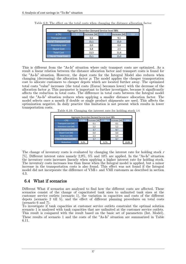
6 Analysis of cost savings in “To-Be” situation
37
Table 6.9: The effect on the total costs when changing the distance a llocation factor
This is different from the “As-Is” situation where only transport costs are optimized. As a result a linear relation between the distance allocation factor and transport costs is found for
the “As-Is” situation. However, the depot costs for the Integral Model also reduces when changing (decreasing) the allocation factor p. The model applies the cheaper transportation cost to allocate customers to cheaper depots which are located further away. The optimized
total costs “value” increases (the total costs (Euros) becomes lower) with the decrease of the allocation factor p. This parameter is important to further investigate, because it significantly affects the reduction in total costs. The difference in total costs between the Integral model
and the “As-Is” situation reduces when applying a smaller distance allocation factor. The model selects once a month if double or single product shipments are used. This affects the optimization negative. In daily practice this limitation is not present which results in lower transportation costs.
Table 6.10: Changing the interest rate for holding stock (r)
The change of inventory costs is evaluated by changing the interest rate for holding stock r [%]. Different interest rates namely 2,9%, 5% and 10% are applied. In the “As-Is” situation the inventory costs increases linearly when applying a higher interest rate for holding stock. The inventory costs increases less than linear when the Integral model is applied, but a minor increase in the transportation costs is also found. This effect was not found if the Integral model did not incorporate the difference of VMI+ and VMI customers as described in section 4.3.
6.4 What if scenarios
Different What if scenarios are analysed to find how the different costs are affected. These scenarios consist of the change of capacitated tank sizes to unlimited tank sizes at the customer service outlets (scenario 1), the variation in capacities and costs of the different depots (scenario 2 till 5), and the effect of different planning procedures on total costs (scenario 6 and 7). To investigate if tank capacities at customer service outlets constraint the optimal solution scenario 1 is analysed with tank capacities that are unlimited at the customer service outlets. This result is compared with the result based on the basic set of parameters (Int. Model).
These results of scenario 1 and the costs of the “As-Is” situation are summarized in Table 6.11.
p [%] 0,5 Increase [k€] 0,7 Increase [k€] 0,9
Transport cost 6,6 9,1
"As-Is" Transport Cost 15,1 15,0
Inventory cost 0,0 0,0
Depot Cost 6,8 2,5
Total Cost 13,3 11,6
"As-Is" Total Cost 15,1 15,0
Aggregate December Demand Service level 98%
r [%] 2,9% Increase [k€] 5% Increase [k€] 10%
Transport cost [k€] 0,1 0,1
Inventory cost [k€] 2,2 5,2
"As-Is" Iventory Cost [k€] 3,7 8,7
Depot Cost [k€] 0,0 0,0
Total Cost [k€] 2,3 5,4
"As-Is" Total Cost [k€] 3,7 8,7
Reduction 9,2% 9,7% 10,8%
Aggregate December Demand Service level 98%

6 Analysis of cost savings in “To-Be” situation
38
Table 6.11: Result scenario 1 and the costs of the “As-Is” situation
The results with the unlimited tank capacities reveal that both the transportation costs and depot costs reduce significantly. This is the result of greater shipment sizes which reduce the transportation costs and thereby the model can allocate the customer service outlets more efficiently in terms of depot costs. However, the inventory costs grow because of the increase in shipment sizes. Note that this situation is not a realistic situation there are always constraints in tank capacity. But the result depicts an optimization possibility. It is expected that the decrease in transportation costs is lower when using route transportation.
Figure 6.4: Costs differences C1 and C2, limited tank capacity and unlimited tank capacity respectively
To clarify the effect described above, an example is given. An end location can be allocated to Depot 1 via link 1 and allocated to Depot 2 via link 2, see Figure 6.4. The red circles represent the optimal shipment size for both links. The figure represents the basic optimization and scenario 1:
Optimal shipment size Link 1 = Q constraint and Optimal shipment size Link 2 > Q constraint
Optimal shipment size Link 1 < Q constraint and Optimal shipment size Link 2 < Q constraint
The cost difference C1 for the basic optimization is much bigger than the costs difference for
Scenario 1, depicted in Figure 6.4, C1>>C2. Too small tanks constrain the allocation possibilities and as a result increases the transportation and depot cost. In scenario 2 the greatest depot in allocated volume, which is also the cheapest depot (one out of 14 depots) is assumed to have limited capacity of 100m3 for each product. In scenario 3 depots located in the whole Rotterdam area are closed. In scenario 4 one out of two depots in the Rotterdam harbour area is closed and the other depot reduces the throughput prices with about 70%. In scenario 5 an extreme scenario is investigated by assuming a throughput price of 0 for the depot in Utrecht. The results of scenario 2 till 5 are summarized in Table 6.12.
Table 6.12: Results of Scenario 2 till 5
When comparing the results of scenario 2 (constraint depot number 4, 100m3) according to Table 6.1 with the Integral model and basic set of parameters a reduction of 6% in the transportation costs is found. The model allocates to nearby depots and thereby reduces transportation costs. The depot costs increases with 13%, because the cheapest depot is
"As Is" Int. Model (Basic) Unlimited Tank capacity Difference
Transport cost [k€] -17%
Inventory cost [k€] 41%
Depot Cost [k€] -10%
Total Cost [k€] -13%
As-Is reduction 9,2% 20,6%
Scenario 1
Int. Model (Basic) DifferenceBP en
Shell 0m3Difference Difference Utrecht free Difference
Transport cost [k€] -6% 37% 18% 27%
Inventory cost [k€] 0% 0% 0% 0%
Depot Cost [k€] 13% 25% -55% -84%
Total Cost [k€] 3% 30% -17% -26%
Scenario 2 Scenario 3 Scenario 5Scenario 4

6 Analysis of cost savings in “To-Be” situation
39
constraint and volume is allocated to depots that are more expensive. The constraint on the cheapest depot generates higher total costs. Scenario 3 discusses the situation where the depots located in the whole Rotterdam area are closed. In this area the cheapest depot is located. All customers in the Rotterdam area are allocated to other further away depots. As a result the transportation cost increases and also the depot cost increases. The depots in the Rotterdam area are very important for Argos and a huge effect on the total costs is generated when closing these depots. In scenario 4 where one out of two depots in the Rotterdam harbour area is closed and the other depot reduces the throughput prices with about 70%. This is however an extreme case, but depicts the effect when greater volume contracts are applied with a much lower throughput price. The transportation costs increases, the model allocates more customer service outlets to the cheaper depot and more kilometres are travelled. The depot costs reduce dramatically. No effect is observed for the inventory costs. The total cost reduces very greatly.
In scenario 5 an extreme scenario is investigated by assuming a throughput price of €0 for the depot in Utrecht (no. 14). Regardless the depot costs of Utrecht are zero still some depot costs are generated, the depot is in some cases too far away from the customers to change the allocation. In that case the transportation costs to Utrecht are higher than the sum of the transportation and depots costs in the chosen allocation. Almost all customers from Rotterdam and other regions are allocated to Utrecht which significantly affects the transportation costs. This effect is clearly shown in Figure 6.5.
Figure 6.5: Loaded volume percentages per product type for Basic optimization (left) and Scenario 5 (right) depot cost of location 14 (Utrecht) is zero.
Different planning procedures are applied in scenario 6 and 7 to investigate the effect of the length of the Lead-Time and review period on the total costs respectively. Two different scenarios of lead-time reduction are applied. The basic set applied in the Integral model is used as comparison. In the basic set the review period (R) is 1 day, Maximum lead-time (L) of 1,5 days and an expected lead-time (l) of 1 day is applied. In scenario 6 the maximum lead-time is reduced to 1 day and the expected lead-time is reduced to 0,75 days. This implies a change of planning in one shift instead of two shifts assumed in the Basic optimization. In Scenario 7 also the review period is reduced to 0,5 days which implies two planning moments per day. The different costs found are depicted in Table 6.13.
Table 6.13: Impact of change planning procedure in scenario 6 and 7
In both scenarios 6 and 7 a reduction is achieved in the transportation, the inventory and depot costs. The safety stocks reduce and as a result the maximum shipment sizes increase when the lead times become smaller. The larger maximum shipment sizes are used to reduce the transportation costs, a larger shipment size reduces the number of times a customer is served. With the reduction of transportation costs the model is able to allocate customer service outlets to cheaper depot locations which are further away to reduce the total costs. The transportation cost reduction is too high for Scenario 6. When changing to one shift the
Int. Model (Basic) Reduction [%] Scenario 6 Reduction [%] Scenario 7
Transport cost [k€] 2,8% 8,8%
Inventory cost [k€] 4,5% 13,1%
Depot Cost [k€] 0,3% 1,2%
Total Cost [k€] 1,7% 5,2%
Total Cost "As-Is" [k€] As-Is reduction 10,7% As-Is reduction 13,9%

6 Analysis of cost savings in “To-Be” situation
40
truck costs will increase and this affect is not corrected in scenario 6. Further research is needed to check if the reduction in costs is greater than the cost increase of less possibilities of clustering orders. Note that the impact is great in size, however it is expected that a change to a specified fraction (P2) will generate less savings for the different planning procedures. As discussed in section 5.2 safety stocks are much smaller when using a P2 probability and the effect of reducing the lead-time is smaller. Also the costs for creating a planning twice a day should be considered in the change in costs. Tank capacities constrain the optimization and as a result safety stock affects the optimization significantly. It is advised to change to a P2 probability and study the effect on the costs in the different scenarios.
6.5 Cost optimization on a yearly basis
To incorporate the variation in demand during the year (month demand differs) also the
total year 2010 is evaluated. The cost on a yearly basis is estimated for the “As-Is” situation and the Integral model is applied with the standard set of parameters. It is explained how the
costs in the “As-Is” situation and the different parameters in the Integral model are
determined. Finally a comparison between the results of the “As-Is” situation and the Integral model is made.
The yearly cost for the “As-Is” situation is created with orders over the year 2010. But the loaded volumes per depot are not validated because of the lack of information. This is only
done for the “As-Is” situation determined on the month December. The allocations are determined with the help of the location IDs used in the validated month December. These IDs where checked (validated) with the loaded volume in that month (December). The total year demand is used to determine the daily demand by dividing the yearly demand by 365 (days). This average daily demand is corrected for a daily pattern and a standard deviation is determined for the variation in the daily demand. Because of the limited data available the calculated standard deviations are converted to correlation variations (C.V.). These C.V. values are plotted against the average demand of the location to investigate if there is a pattern when increasing or decreasing the demand of a service location. For the products Gasoline (Euro) and Diesel the C.V. are determined for two volume classes. These C.V. classes are used to determine the standard deviation for the customers where the daily demand data was not available. The data depict that there is a higher C.V. for low demand locations in comparison with a smaller C.V. for greater demand locations.
Table 6.14: “As-Is” costs for 2010 and results Integral model with basic set of parameters
The results of the different costs for the “As-Is” situation and the Integral model are
summarized in Table 6.14. The calculated total costs per year are ''''''''''''''''''',= and this is
lower than '''''''''''''''''''' '''''''''''''''''''''' 12 times the determined December costs. This is the result of the variation in demand over the months. The found savings in costs (%) are comparable to the savings summarized in Table 6.6 which are based on the orders in the month December. A reduction in total costs of 8,5% is found and this reduction is mainly caused by the lower transportation and depot costs. The reduction in depot costs is the result of the allocation of cheaper depots. This affects the distribution of the loaded volumes at the different depots significantly.
2010 "As-Is" Distri. Int. Model (Basic) Reduction
Yearly Transpot cost [k€] 50,9% 9,3%
Yearly Inventory cost [k€] 2,6% 33,4%
Yearly Depot Cost [k€] 46,5% 6,4%
Yearly Total Cost [k€] 100,0% 8,5%

6 Analysis of cost savings in “To-Be” situation
41
Service level Different service levels at the customer service outlets are applied to investigate the effect of the service level (P1) on the total costs. Two different service levels are applied 99,7% and 98% respectively. The different costs found are depicted in Table 6.15.
Table 6.15: Effect of service level on Total Cost
Different from the month analyses, not only the transportation costs changes significantly, but also the depots cost decreases when reducing the service level. The transportation cost
reduces compared to the “As-Is” situation. This results in a total cost reduction of 6,2% and 7,9% for service levels of 99,7% and 98% respectively. The effect on the inventory costs is marginally, because of a low interest rate for holding stock (2,98%) is applied. Recommendation to further reduce safety stocks The safety stocks are calculated via a P1 probability, however also the possibility of a P2 probability is discussed. The P1 probability used in the inventory policy creates higher safety stocks then needed to assure the service level P2 during the year. An example is given to show the reduction of safety stock possibility:
326,25 Q m , 31,5 L R m and
35 L Rh m
3
1( 99%) 2,71 1,5 4,07 L RSS P k m
For P2 first formula needs to be calculated:
2
26,25( ) 1 1 0,99 0,175 k= 0,58
1,5u
L R
QG k P
3
2( 99%) 0,58 1,5 0,87 L RSS P k m
A big reduction is founded in this example and using a P2 probability reduces a lot of safety stock and increases the shipment size which can therefore reduce the transportation costs. As indicated a P1 probability is used to assure the linearity of the model, however to reduce the safety stocks a heuristic is developed to change the P1 probability to a P2 probability. Module 1 first solves the shipment sizes with the P1 probability to determine the shipment sizes Q.
1. First Solve module 1 with a chosen P1-value which is the same as desired P2-value 2. Use the calculated Shipment sizes for all the combinations and calculate the needed
Gu(k) value by the chosen service level P1=P2 in function (6.4) (Silver et.al. 1998).
2( ) 1 (6.4)u
L R
QG k P
3. Then k-values are calculated via the use of an Excel function. 4. Use the calculated k-values in all combinations and solve module 2 again. The
locations with a bigger shipment size will have more available tank space. The shipment sizes are solved and are increased. Step 2 and 3 can be repeated more times to assure an optimal solution.
The heuristic is not used in the module 1, but is easily incorporated. The company needs to check which service measure to use P1 or P2. For now the P1 probability is used in the thesis.
"As-Is" Costs (P1) 99,7% Reduction of "As-Is" (P1) 98% Reduction of "As-Is"
Transport cost [k€] 6,6% 9,3%
Inventory cost [k€] 31,3% 33,4%
Depot Cost [k€] 5,6% 6,4%
Total Cost [k€] 6,8% 8,5%
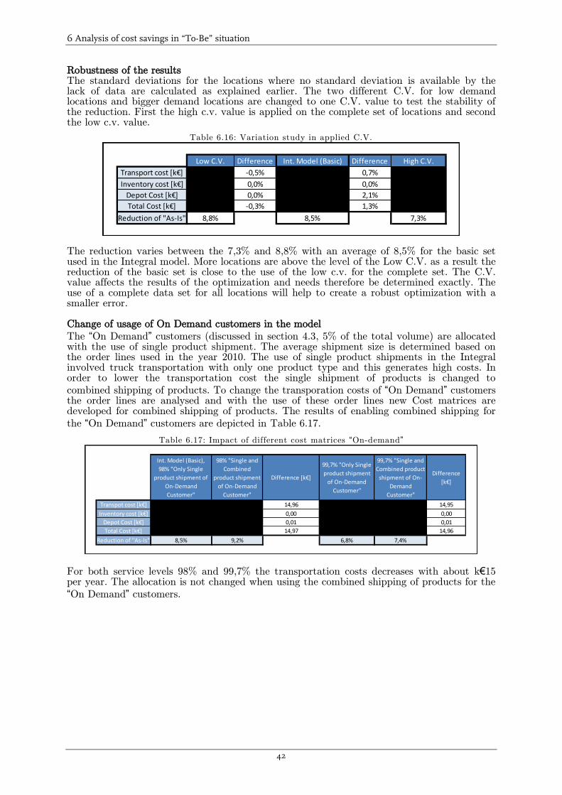
6 Analysis of cost savings in “To-Be” situation
42
Robustness of the results The standard deviations for the locations where no standard deviation is available by the lack of data are calculated as explained earlier. The two different C.V. for low demand locations and bigger demand locations are changed to one C.V. value to test the stability of the reduction. First the high c.v. value is applied on the complete set of locations and second the low c.v. value.
Table 6.16: Variation study in applied C.V.
The reduction varies between the 7,3% and 8,8% with an average of 8,5% for the basic set used in the Integral model. More locations are above the level of the Low C.V. as a result the reduction of the basic set is close to the use of the low c.v. for the complete set. The C.V. value affects the results of the optimization and needs therefore be determined exactly. The use of a complete data set for all locations will help to create a robust optimization with a smaller error. Change of usage of On Demand customers in the model
The “On Demand” customers (discussed in section 4.3, 5% of the total volume) are allocated with the use of single product shipment. The average shipment size is determined based on the order lines used in the year 2010. The use of single product shipments in the Integral involved truck transportation with only one product type and this generates high costs. In order to lower the transportation cost the single shipment of products is changed to
combined shipping of products. To change the transporation costs of “On Demand” customers the order lines are analysed and with the use of these order lines new Cost matrices are developed for combined shipping of products. The results of enabling combined shipping for
the “On Demand” customers are depicted in Table 6.17.
Table 6.17: Impact of different cost matrices “On-demand”
For both service levels 98% and 99,7% the transportation costs decreases with about k€15 per year. The allocation is not changed when using the combined shipping of products for the
“On Demand” customers.
Low C.V. Difference Int. Model (Basic) Difference High C.V.
Transport cost [k€] -0,5% 0,7%
Inventory cost [k€] 0,0% 0,0%
Depot Cost [k€] 0,0% 2,1%
Total Cost [k€] -0,3% 1,3%
Reduction of "As-Is" 8,8% 8,5% 7,3%
Int. Model (Basic),
98% "Only Single
product shipment of
On-Demand
Customer"
98% "Single and
Combined
product shipment
of On-Demand
Customer"
Difference [k€]
99,7% "Only Single
product shipment
of On-Demand
Customer"
99,7% "Single and
Combined product
shipment of On-
Demand
Customer"
Difference
[k€]
Transpot cost [k€] 14,96 14,95
Inventory cost [k€] 0,00 0,00
Depot Cost [k€] 0,01 0,01
Total Cost [k€] 14,97 14,96
Reduction of "As-Is" 8,5% 9,2% 6,8% 7,4%
6 Analysis of cost savings in “To-Be” situation
43
6.6 Conclusion
The Integral model is applied to optimize the total costs that comprises transportation, depot
and inventory costs. First, the costs in the “As-Is” situation are determined. These costs are compared with the results of the Integral Model. For both models the demand per product based on all orders in the month December and the loading locations are used to determine the costs. The majority of the calculations with the Integral model are carried out with a basic set of parameters described in section 6.2. The daily demand is analysed and the daily pattern is taken into account by multiplying the average day demand with a day index. To analyse the variation in daily demand coefficients of variation (C.V.) are determined for 2 products respectively diesel and gasoline. Based on the results it is decided to divide the C.V. in two volume classes. Locations with a month demand lower than 50m3 have a high average C.V. and a lower average C.V. is applied for a month demand greater than 50m3. A
reduction of 9% in the total costs is found with the Integral model compared to the “As-Is” situation. The Integral model is used to investigate the effect on the optimization if different throughput prices, service levels, distance allocation factors and the capacities of the different tanks at the customer service outlets are varied. In total 7 different What If scenarios are analysed to show how the different costs are affected. These scenarios comprise the change of capacitated tank sizes at the customer service outlets, the variation in capacities and costs of the different depots and the effect of different planning procedures on the total cost. The constraint tanks at the customers service outlets reduce the optimization possibilities with a great extent.
The yearly cost for the “As-Is” situation is determined with orders in the year 2010. In this way the actual year demand is taken into account and a reduction on the total year costs of 8,5% is achieved. Also the effect of different service levels and C.V. values are studied.
The “On-Demand” customers are allocated with the use of a single product shipment. New cost matrices are developed for combined shipment of products. Enabling combined shipping
for the “On-Demand” customers result in a small decrease of the transportation costs of about
k€15 a year. With the aid of the forecasted volume new volume contracts can be determined in cooperation with the Wholesale department. With these forecasts the Wholesale department knows how much volume is needed for the supply chain per depot. It is advised to manage
the volume contracts by changing loaded volumes of the “Ex-Works” customers per depot via pricing or fixed volume contracts.

44
7 Conclusion and Recommendations
In this study a model is developed to analyse and optimize the structure of a distribution Supply Chain. Different departments namely, Wholesale, Logistics and Retail play a role in the distribution Supply Chain of Argos. These departments work currently independent of each other and that prevents a total cost optimization. No insight in the relationships between depot costs, inventory costs and transport costs are known. For that reason the main objective of this project is:
Develop a method to analyse and optimize the structure of a distribution supply chain, which consist of demand allocation decisions, transportation decisions and inventory decisions, while taken into account flow capacity constraints and tank sizes.
In order to gain insight into the various costs and the suggested improvements an Integral model is developed. The found models in the literature lack the incorporation of safety stocks, throughput costs of different depots and use a too general transportation cost function. For that reason a new Integral model is developed that incorporates the mentioned gaps namely: safety stocks at the service outlets, different throughput costs, and a transportation cost function that is based on distance and carried load. The Integral model takes into account the maximum truck load and the maximum shipment size in relation to the tank capacity at the customer service outlets. The Integral model optimizes the total costs that consist of transportation costs, depot costs and inventory costs. In order to find the effect on the optimization of the total costs, the following parameters are varied; throughput prices, service level, distance costs and capacities of different tanks at the
customer service outlets. The results of the optimization are compared with the “As-Is”
situation. Furthermore different “What If” scenarios and planning procedures are applied to investigate the effect on the total costs. Based on the results of this study the following conclusions are drawn:
An Integral model is developed that optimizes the total costs that comprises transportation, inventory and depot costs. The reduction in total costs based on the loaded volumes in the month December 2010 amounts to about 9% compared to the
“As-Is” situation. The reduction is mainly caused by the lower transportation about 11% and depot costs 5% and is achieved if no capacity constraints for the different depots exist.
The optimization shows that the distribution of the loaded volumes at the different depots changes dramatically and is concentrated in a depot location in Rotterdam for 50% (gasoline and diesel) to 80% (gasoil).
The inventory costs are reduced with about 35% if a probability of no stock during the replenishment cycle of 98% (P1) for all tanks is applied. However, the inventory cost is responsible for a minor part 3% of the total cost in the Distribution Supply Chain.
The found reduction on inventory costs is marginally when changing to a planning which distinct between customer service outlets with and without inventory cost for Argos. The interest rate used by Argos is small and therefore transport costs are more important than inventory cost. The optimal delivery size is in most cases the maximum tank capacity.
With the Integral model the effect of different service levels (that specifies the probability of no stock out during the replenishment cycle) on the total costs is calculated. With this approach average stocks are minimized at the Retail service outlets with more than 30%. Furthermore, the maximum shipment sizes decreases when increasing the service level (safety stock) at customer service outlets.
The allocation of the customer service outlets to the different depots depends not only on the transportation costs but on the total cost of transportation, depot and inventory.
The Integral model is able to handle extreme “What If” scenarios. It can be used as a tool to take into account the effects of e.g. a change in throughput prices and closing or opening depots.
7 Conclusion and Recommendations
45
The model can be used by the Wholesale department to generate monthly forecasts with the chosen allocation of customers. The Logistics department can use the tool to
investigate different What If scenarios and show the impact on the total cost.
Recommendations Transport The transport cost function used in the Integral model is a slightly adapted version of direct transportation cost. Loading and unloading times are assigned correctly. However the distance cost is not correct for the use in route transportation. In reality a truck follows a route and visits various customers. The distance cost varies in that case with the number of other customers on the route. The number of customers varies with the shipment size of a customer. It is advised to analyse the chosen shipment sizes of the Integral model in daily planning program (VRP). When using a VRP for simulations it is possible to get deeper insights in the actual transportation costs when changing the shipment size for multiple locations. The model can be improved by including different types of trucks, various locations are better served with a smaller truck. The created solutions with the Integral model give a basic set of allocations. Starting from this basic set of allocations it is easier to check if multiple customers can be applied on a route economically. Inventory The different calculated trigger levels s and safety stocks can be used by Argos directly. It is however advised to change the used model for the incorporation of undershoots. The incorporation of undershoots can reduce needed safety stock. Safety stocks and transportation costs can be reduced dramatically when changing the P1 probability to a P25 probability. The P2 probability is not only based on the replenishment cycle and thereby safety stocks needed are smaller for a good service level. The change to two planning moments reduces the total cost and it is advised to do more research in the extra costs for applying two planning moments per day. The use of can-orders can reduce the costs of transportation to create clusters of customers. The model needs to be expanded for variable lead-times, this will reduce needed safety stocks. The data of lead-times should be analysed to fit a distribution. A uniform distribution is expected, using the simple incorporation of lead-time via the normal distribution will result in to big safety stocks and is not advised. Maximum lead times are used in the present model. Practical recommendations for Argos Multiple parameters are based on interviews, because the lack of data did not allow validating the parameters e.g. pomp speed for the unloading times per customer or depot. Average values are used for all locations. The Integral model will create better results when using complete data sets. It is advised to create a data management system, where different parameters are measured. It is easier to analyse the complete Supply chain of Argos with the help of such a system. It is advised to apply the model for the Supply Chain of LPG (BK-Gas), because the throughput prices of the depots differ significantly. These differences in throughput prices are greater than the throughput price differences of gasoline, diesel and gasoil. As a result the model will generate higher savings compared to the achieved savings e.g. gasoline and diesel. It is recommended to change from a P1 probability to a P2 probability. A heuristic is given to expand the created model to incorporate the P2 probability. Model expansions The average truck speed can vary per link from depot location to customer. In the model only one average transportation speed is used. It is advised to apply a more accurate average transport speed for each link. The inventory policy needs to be adapted for the customer locations with delivery time windows. The expected lead times are more accurate in this case. The (un)loading times are based on average values. However, different values for each location (depot and customer) can be used in the model to predict the costs more accurately. Moreover, it can affect the depot allocation choice.
5 Specified Fraction of Demand to Be Satisfied Routinely from the Tank

46
8 References
Amiri, A. (2006), “Designing a distribution network in a supply chain system: Formulation
and efficient solution procedure”, European Journal of Operational Research, Vol. 171, Iss: 2, 1 June 2006, pp.567-576, Nr of Cit. 69
Battin, D. (2008), “Dynamic modelling of networks and logistic complex systems”, Phd thesis, Department of management and Engineering - Italy, pp. 20-69
Baumol, W.J. and Vinod, H.D. (1970), “An Inventory Theoretic Model of Freight Transport
Demand”, Management Science, Vol.16, No. 7, Theory Series (Mar., 1970), pp. 413-421, Nr of Cit. 151
Bertrand, J.W.M., Fransoo, J.C., (2002), “Operations Management Methodologies Using
Quantitative Modeling”, International Journal of Operations & Production Management 22(2), pp. 41-264,Nr. Of cit. 114
Chopra, S. (2003), “Designing the distribution network in a supply chain”, Transportation Research Part E: Logistics and Transportation Review, Vol. 39, Iss: 2, March 2003, pp. 123-140, Nr of Cit. 77 Chima, C. M. (2007),“Supply-Chain Management issues in the oil and gas industry”,Journal of Business & Economics, Vol. 5, No. 6, pp. 27-36, Nr. Of Cit. 3 Constable, G.K. and Whybark, D.C. (1978), “The Interaction of Transportation and
Inventory Decsions”, Decisions Sciences, Vol. 9, Iss. 4, pp. 688-699, October 1978, Nr of Cit. 39
Daganzo, C.F. (2005), “Logistics systems analysis”, Springer, Berlin, Nr.Of cit. 241
De Kok, A.G. and Fransoo, J.C. (2003), “Chapter 12: Planning Supply Chain Operations: Definition and Comparison of Planning Concepts, Eds., Handbooks in OR & MS, Vol. 11, pp. 597-675, Nr. Of cit. 57 De Kok, A.G., (2005), “Analysis of stock control models for one location with one product”, Handout Stock Control, Reader Logistics 1 course, Eindhoven University of Technology Ghiani, G., Laporte, G. and Musmanno, R.(2004), “Introduction to Logistics Systems
Planning and Control”, Wiley, Chichester, England (2004).Nr. Of cit. 137 Hakimi, S.L. (1964), “Optimum locations of switching centers and the absolute centers and
medians of a graph”, Operations Research, Vol. 12, No. 3, May-Jun 1964, pp. 450-459, Nr of Cit. 894
Hussain, R., Assavapokee, T. and Khumawala, B. (2006).“Supply Chain Management in the
Petroleum Industry: Challenges and Opportunities”, International Journal of Global Logistics & Supply Chain Management , Vol. 1, No. 2, pp. 90-97, 1 November 2006, Nr. Of Cit. 2
Jayaraman, V. (1998), “Transportation, facility location and inventory issues in distribution
network design: An investigation”, International Journal of Operations & Production Management, Vol. 18, Iss: 5, pp. 471-494, Nr of Cit. 66
Lee, H.L., Padmanabhan, P., Whang, S. (1997), “Information distortion in a supply chain: The bullwhip effect. Management Sci. 43 pg. 546-558, Nr. Of. Cit. 2353

8 References
47
Mitroff, I.L., Betz, F., Pondy, L.R. and Sagasti, F. (1974), “On managing science in the
systems age: two schemas for the study of science as a whole system phenomen”, Interface, Vol.4. No.3, pp. 46-58
Perl and Sirisoponsilp, J. and Sirisoponsilp, S. (1988), “Distribution Networks: Facility
Location, Transportation and Inventory”, International Journal of Physical Distribution & Logistics Management, Vol. 18 Iss: 6, pp. 18-26, Nr of Cit. 22
Puijman, R. (2011), “Buffer and inventory management downstream of a cracker: a queuing
theory approach”, MSc Thesis, TechnischeUniversiteit Eindhoven, pp. 1-13
Schmidt and Wilhelm, G.S. and Wilhelm, W.E. (1999), “Strategic, Tactical and Operational
Decisions in Multi-national Logistics Networks: A Review and Discussion of Modeling Issues”, International Journal of Production Research, Vol. 38, No. 7, 10 May 2000, pp. 1501-1523, , Nr of Cit. 48 Shah, N. (2005), “Process industry supply chains: Advances and challenges”, Computers & Chemical Engineering, Vol.29, Is. 6, pp. 1225-1236, 15 May 2005, Nr. of Cit. 88 Shell, (2011), Schematic overview Upstream and Downstream,ROYAL DUTCH SHELL plc, 2010 investor factsheet, retrieved: http://www-static.shell.com/static/investor/downloads/shell_at_a_glance/2010_ir_factsheet_english.pdf
Shen, Z.M., Qi, L. (2007), “Incorporating inventory and routing costs in strategic location
models”, European Journal of Operation Research, Vol. 179, Iss.2, pp. 372-389, 2007, Nr. Of Cit. 38
Siddharth, V., Subhash, W. and Deshmukh, S.G. (2007), “Supply chain characteristics of the
petroleum industry: The Indian Context”, South Asian Journal of Management, Vol. 14, No. 2, pp. 107, Apr-Jun 2007, Nr. Of Cit. ? Silver, E.A.,Pyke, D.F., Peterson, R. (1998), “Inventory Management and Production
Planning and Scheduling”, New York, Wiley, Nr.Of cit. 1449 Van der Veen, R.C.T., (2011), Design of a distribution supply chain network in the Oil Industry, Eindhoven University of Technology, Literature Review for Master Thesis Preparation (1ML05) Waller, M., Johnson, M.E. and Davis T. “Vendor-managed inventory in the retail”, supply chain. Journal of Business Logistics 20 1 (1999), pp. 183–203, Nr. Of cit. 379

48
Appendix I Combined shipment of two products (part of Module 1)
In this appendix the optimization of the product cost function for combined shipping of two products is explained in detail. This approach to optimize the product cost function only holds for one product type per shipment. For the option, combined shipping with two product types per shipment a different approach is needed. The basic Total Relevant Cost function of serving demand for two product types from depot i and customer service outlet j is determined via the following function:
,
, , , , 1
The Costs of the combined shipmentsizes (c12 )
+ +1 (I.1)
11 1 1 2 2 2
11 1 1 1
2
2
ij
ijmonth j
ij
i j ij i j ij j
ij
L R j l j L R j u j
i
tcp dis kc tch
aspQ
Z lt ut Q lt ut Q ct
Qh h k x v
Q
, , , , 22 2 2 22
month
j
L R j l j L R j u j
r
h h k x v
1 1 2 2 1 21 1 2 2 if
1 2 otherwise
ij ij ij ijiij ij
iij ij
Q Q Q QdtQ Q
ttw ttw ttvZ
dtQ Q
ttv
The product cost function is depicted in equation (I.1) for the combination of product 1 and product 2. The function is identical for the combination of product 2 and 3 only the numbers 1 and 2 in equation (I.1) are changed to numbers 2 and 3 respectively. The problem to solve is that with combined shipments the tanks should be replenished on the same time, resulting in a replenishment time of product 1 equal to replenishment time of product 2. In other words the tanks need to be synchronized. To determine the shipment sizes for this synchronization multiple steps are needed. The problem changes to two separate problems with inventory costs for the company Argos and without inventory costs for the company Argos. The solution method is discussed that is valid for the product cost function with inventory costs for Argos. To consider this the optimal shipment sizes are calculated via the use of calculus (differentiation), such as the approach applied to find the optimal single product
solution. The approach is slightly adapted by adding a factor α in equation (I.2) to make it possible to share the fixed costs. The used function is depicted in equation (I.2) and is needed to synchronize the replenishment time.
1 2
1 2Optimal time:
1 2
2 2 1
(I.2)1 2
ij ij
i i
i ij i ij
i i
q q
h h
tc tcCT tc p Dis kc CT tc p Dis kc
ASP ASP
h v r h v r
1 0ih and
2 0ih
1
1 2
1
1 2
i
i i
h v
h v h v
Equation (I.3) depicts the found optimal shipment sizes q1ij and q2ij for combined shipping without constraints.

0 Appendix I Combined shipment of two products (part of Module 1)
49
*
1
*
2
2 1
1
2 2 1
2 (I.3)
i i ij
ij
i i ij
ij
tch CT tc p Dis kc
ASPq
v r
tch CT tc p Dis kc
ASPq
v r
As discussed the approach described above does not take into account the different shipment size constraints. To integrate these constraints a LP solution is applied, which solves the shipment size for multiple end locations that are supplied with one single depot:
max j
j
X (I.4)
Subject to: * (I.4a)j j j
j
X q1 q1max
* 1 (I.4b)j j j
j
X q1 h
*2 2 (I.4c)j j j
j
X q q max
*2 2 (I.4d)j j j
j
X q h
* *1 1 2 2 (I.4e)j j j
j
X q q TTW
* *1 2 (I.4f)j j j
j
X q q TTV
1 (I.4g)jX
As a result of the formulated constraints the LP tends to keep both the shipment sizes (optimal shipment sizes) as great as possible. Note that the shipment sizes cannot be larger as found by the unconstrained function (I.3). The calculated shipment sizes of function (I.3) are q1j
* and q2j *. Comparable to the formulation of the single product cost function the
shipment size is constraint by the month/year demand h1j and h2j in constraints (I.4b) and (I.4d). The shipment sizes are constraint by the available tank capacity for product 1 represented by constraint (I.4a) and for product two by constraint (I.4c). The shipment sizes are constraint by the maximum truck weight via constraint (I.4e). To fulfil this constraint
the densities 1 and 2 , product 1 and product 2 respectively are included. Constraint
(I.4f) confines the shipment sizes in relation to the associated maximum truck volumes. Constraint (I.4g) assures that the maximum shipment sizes are not larger than calculated via function (I.3). The LP optimizes one depot i combination each time and needs to be carried out again for the number of depots. First for i=1 till N (number of depots). The locations without inventory costs for Argos are also optimized for combined shipping. For the locations without inventory cost for Argos (VMI), a different optimization is needed compared to the found solution valid for the product cost function with inventory cost. When there is no inventory cost, the shipment size needs to be as big as possible. However, the replenishment times must be equal for both products on the aggregate level. This requirement is formulated in equation (I.5) where the optimal replenishment time is calculated.
1 2Optimal time: (I.5)
1 2
ij ij
i i
q q
h h
For this problem also a LP is applied to take into account the tank capacity constraint and the maximum truck weight constraints, see equations (I.6) to (I.6g).

0 Appendix I Combined shipment of two products (part of Module 1)
50
1 2max (I.6)
1 2
j j
j j j
Q Q
h h
Subject to:
(I.6a)j j
j
Q1 q1max
1 (I.6b)j j
j
Q1 h
2 2 (I.6c)j j
j
Q q max
2 2 (I.6d)j j
j
Q h
1 2 (I.6e)
1 2
j j
j j j
Q Q
h h
1 1 2 2 (I.6f)j j
j
Q Q TTW
1 2 (I.6g)j j
j
Q Q TTV
The synchronization of the delivery times is assured with constraint formulated in equation (I.6e). The shipment size is constrained by the month/year demand h1j and h2j in constraints (I.6b) and (I.6d). The shipment sizes are restricted by the available tank capacity for product 1 by constraint (I.6a) and for product two by constraint (I.6c). The shipment sizes are
constrained by the truck weight via constrained (I.6f). To do this the densities 1 and 2
of product 1 and product 2 respectively are included. Constraint (I.6g) takes into account the maximum truck volumes for the shipment sizes.
Both LP’s solve the constraints in the multiple product type shipment. The calculated shipment sizes are an input for the different cost functions. A good distinction is needed between the location with inventory costs of Argos and those without inventory costs of Argos. In contrast with the LP for the customers with inventory costs the LP without inventory cost only needs to be carried out once. The shipment size does not change with the allocation. Greater shipment sizes are always cheaper in this case for Argos.
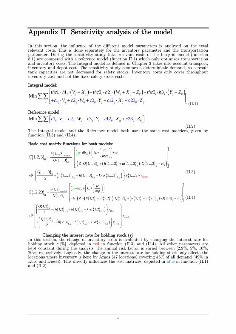
51
Appendix II Sensitivity analysis of the model
In this section, the influence of the different model parameters is analysed on the total relevant costs. This is done separately for the inventory parameter and the transportation parameter. During the sensitivity study total relevant costs of the Integral model (function 8.1) are compared with a reference model (function II.1) which only optimizes transportation and inventory costs. The Integral model as defined in Chapter 3 takes into account transport, inventory and depot cost. The sensitivity study assumes a deterministic demand, as a result tank capacities are not decreased for safety stocks. Inventory costs only cover throughput inventory cost and not the fixed safety stock costs. Integral model:
1
1 1 2 2 3 3M
2 3 12 3i
2n
i j ij ij i j ij ij ij i j ij ij
i j ij ijij ij ij iji jj ij iji
thc h V X thc h W X Z thc h Y Z
Vc c c c cW Y X Z
(II.1)
Reference model:
1 2 3 1n 2 2Mi 3ij ij ij ij iij ij ij ij ij j
i j
V W Y X Zc c c c c (II.2)
The Integral model and the Reference model both uses the same cost matrices, given by function (II.3) and (II.4). Basic cost matrix functions for both models:
,
, , ,
+ +1,..,3
1,..,31,..,3 1,..,3 1,..,3 1,..,3
1,..,31,..,3 1,..,3 1,..,3 1,..,3
2
1,2,3ij
month j
ij
jij i j ij
ij
L j l j L j month
ij
r
tcdis kc tch
asp
QZ Q lt ut Q ct
Qh h k v
p
C
(II.3)
,
1,2, , ,
, , ,
+1,2
1,2+ 1,2 1,2 1,2 2,3 2,3 2,3
1,21,2 1,2 1,2
2
2,32,3 2,3 2,3
2
C 12,23ij
month j
ij
ji j ij i j ij
ij
L j l j L j
ij
L j l j L
ij
tcdis kch
asp
Qtc Z lt ut Q lt ut Q ct
Qh h k v
Qh h k
p
2,3
mo
j
nthr
v
(II.4)
Changing the interest rate for holding stock (r)
In this section, the change of inventory costs is evaluated by changing the interest rate for holding stock r [%], depicted in red in function (II.3) and (II.4). All other parameters are kept constant during the analysis, the annual risk factor is varied between [2,9%; 5%; 10%; 20%] respectively. Logically, the change in the interest rate for holding stock only affects the locations where inventory is kept by Argos (47 locations) covering 46% of all demand (49% in Euro and Diesel). This directly influences the cost matrices, depicted in blue in function (II.1) and (II.2).
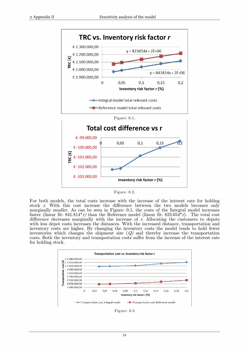
0 Appendix II Sensitivity analysis of the model
52
Figure: 0.1,
Figure: 0.2,
For both models, the total costs increase with the increase of the interest rate for holding stock r. With this cost increase the difference between the two models becomes only marginally smaller. As can be seen in Figure: 0.1, the costs of the Integral model increases faster (linear fit: 841.814*r) than the Reference model (linear fit: 823.654*r). The total cost difference decreases marginally with the increase of r. Allocating the customers to depots with less depot costs increases the distances. With the increased distance, transportation and inventory costs are higher. By changing the inventory costs the model tends to hold fewer inventories which changes the shipment size (Q) and thereby increase the transportation costs. Both the inventory and transportation costs suffer from the increase of the interest rate for holding stock.
Figure: 0.3
€ -103.000,00
€ -102.000,00
€ -101.000,00
€ -100.000,00
€ -99.000,00
0 0,05 0,1 0,15 0,2
TRC
[€
]
Inventory risk factor r (%)
Total cost difference vs r

0 Appendix II Sensitivity analysis of the model
53
Figure: 0.4
When looking at the transportation cost in Figure: 0.3, a larger increase is measured for the Integral model. This is a result of the greater distance driven when using a total optimization. The transportation costs increase with a higher amplitude when the interest rate for holding stock is increased from 10% till 20%. Figure: 0.4, represents the total inventory costs versus the interest rate for holding stock. The inventory costs increase linearly (the green line is a linear cost function) when the risk factor is varied between 2.9% and 10%. When increasing the risk factor more than 10%, the inventory costs increase less than linear, because the model decreases the shipment size. Normally, the increase would not be a linear line, this can be explained by the constraints e.g., tank size at end locations and truck capacity. For an interest rate for holding stock of 2,9% till 10% the on average optimal shipment size is bigger than the restriction size, for 15% and 20% the optimal shipment size is less than the restriction size. This explains the end of the almost linear line. This will be further discussed later.
Figure: 0.5
The depot costs are depicted in Figure: 0.5. The depot cost is intuitively the same for the basic model without depot costs optimization. However, the depot costs for the total optimization change at an interest rate for holding stock of 15%. When changing the interest rate for holding stock the optimal shipment size also changes. As seen in Figure: 0.3, the transportation cost increases at a risk factor of 15%, which justifies a smaller shipment size and/or an increase in travelled distance. A nearby allocation will have a smaller shipment size, which keeps the balance of transportation cost and inventory costs low. A allocation further away increases the shipment size to reduce the transportation cost in comparison with the inventory cost.
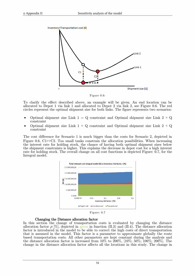
0 Appendix II Sensitivity analysis of the model
54
Figure 0.6:
To clarify the effect described above, an example will be given. An end location can be allocated to Depot 1 via link 1 and allocated to Depot 2 via link 2, see Figure 0.6. The red circles represent the optimal shipment size for both links. The figure represents two scenarios:
Optimal shipment size Link 1 = Q constraint and Optimal shipment size Link 2 > Q constraint
Optimal shipment size Link 1 < Q constraint and Optimal shipment size Link 2 < Q constraint
The cost difference for Scenario 1 is much bigger than the costs for Scenario 2, depicted in
Figure 0.6, C1>>C2. Too small tanks constrain the allocation possibilities. When increasing the interest rate for holding stock, the chance of having both optimal shipment sizes below the shipment constraints is higher. This explains the decrease in depot cost for a high interest rate for holding stock. The overall change on all cost functions is depicted Figure: 0.7, for the Integral model.
Figure: 0.7
Changing the Distance allocation factor
In this section the change of transportation costs is evaluated by changing the distance allocation factor p [%], depicted in green in function (II.3) and (II.4). The distance allocation factor is introduced in the model to be able to correct the high costs of direct transportation that is assumed in the model. This factor is a parameter to approximate globally the route based transportation costs. All other parameters are kept constant during the analysis and the distance allocation factor is increased from 10% to 200%, [10%; 50%; 100%; 200%]. The change in the distance allocation factor affects all the locations in this study. The change in

0 Appendix II Sensitivity analysis of the model
55
the distance allocation factor directly influences the cost matrixes, depicted in blue in function (II.1) and (II.2).
Figure: 0.8
Figure: 0.9
For both models the total costs increases with the increase of the distance allocation factor p. It is found that the difference in total costs between the two models vanishes for larger
distance allocation factors. As can be seen in Figure: 0.8, the total costs of the ‘integral
optimization model’, represented by the blue line, increases faster than the total cost of the Reference, represented by the red line. The total cost difference between the two models reduces with the increase of the distance allocation factor p, depicted in Figure: 0.9. Allocating the customers to depots with less depot costs increases the distances. With the increased distance transportation costs are higher. By increasing the transportation cost, the model will try to minimize travelled distance and number of times travelled. As a result, the model will try to change the shipment size (Q) and thereby increases the inventory costs and/or changes the allocation. Both the inventory and transportation costs suffer from the increase of the distance allocation factor p.

0 Appendix II Sensitivity analysis of the model
56
Figure: 0.10
The transportation costs increases with the increase of the distance allocation factor p, depicted in Figure: 0.10. The transportation cost increase linear for the Reference model, which only optimizes inventory and transportation costs, represented by the red line. However, the transportation costs of the integral model, represented by the blue line, are
significantly higher for a distance allocation factor below 1,0. The ‘integral optimization
model’ will create higher travel distances when the allocation factor p is decreased. Some may wonder why the transportation costs are almost equal at a distance allocation factor of 0,1. This is because the travelled distance costs are almost zero and the fixed (un)loading costs remain constant.
Figure: 0.11
A similar effect as shown in the transportation cost graph, depicted in Figure: 0.10, can be seen on the inventory cost graph, depicted in Figure: 0.11. When an allocation factor of 0,5 is applied in the models, the inventory cost is for the integral model higher compared with the reference model. When the allocation factor is below 1,0 there is more space for optimization. Tank capacities are less likely to be a constraint. When the allocation factor is above 1,0, the tanks are completely full and the inventory cost increase linearly.

0 Appendix II Sensitivity analysis of the model
57
Figure: 0.12
The transportation and inventory graphs indicate high savings on depot costs for allocation factors below 1,0. Figure: 0.12 depicts the Depot cost versus the distance allocation factor p. As expected, the depot cost of the Integral model decreases with high amplitude when decreasing the distance allocation factor. Changing the distance allocation factor to correct
for the direct transport assumption has a big impact on the optimization ‘value’ of the Integral model. The overall change on all cost functions is depicted Figure: 0.13, for the Integral model.
Figure: 0.13

0 Appendix II Sensitivity analysis of the model
58
Figure: 0.14
The distance allocation factor, has an impact on the transportation, inventory and depot cost. The total optimization creates a higher value, when decreasing the distance allocation factor. The effect on the shipment size is depicted in Figure: 0.14.
Impact of constrained tanks at end locations
In the former sections, the problem of tank capacities is raised multiple times. A comparison is made between an un-capacitated case and capacitated case, to show that the total costs are really affected to a great extent.
Figure: 0.15
Figure: 0.15, depicts the costs of the capacitated case and the un-capacitated case, reflected with number 1 and 2 respectively. The total costs are for both models smaller in the un-
capacitated case, but the decrease in costs is greater for the ‘integral model’ (linear fit: -6318*{1,2} vs. linear fit: -4987*{1,2} ). The Integral model tends to keep more inventories to be able to travel larger distances. Whereas the reference model only uses the extra tank space to create an optimal shipment size.

0 Appendix II Sensitivity analysis of the model
59
Conclusion Different parameters are varied in the sensitivity study. The most important implications are:
An increase in the interest rate for holding stock, greatly affects the transportation and inventory costs. The depot costs remains nearly constant when changing the interest rate for holding stock. The total value of the integral model only suffers marginally by changing interest rate for holding stock.
A decrease in the distance allocation factor, has an impact on the transportation, inventory and depot cost. The total optimization creates a higher value, when decreasing the distance allocation factor.
Tank capacities constrain the optimization significantly. An optimization effort exists for Argos to change tank capacities at end locations. This could imply switching tanks between Euro and Diesel at the Service Outlets.
60
Appendix III Basic set of parameters
CONFIDENTAIL

61
Appendix IV Integral Model
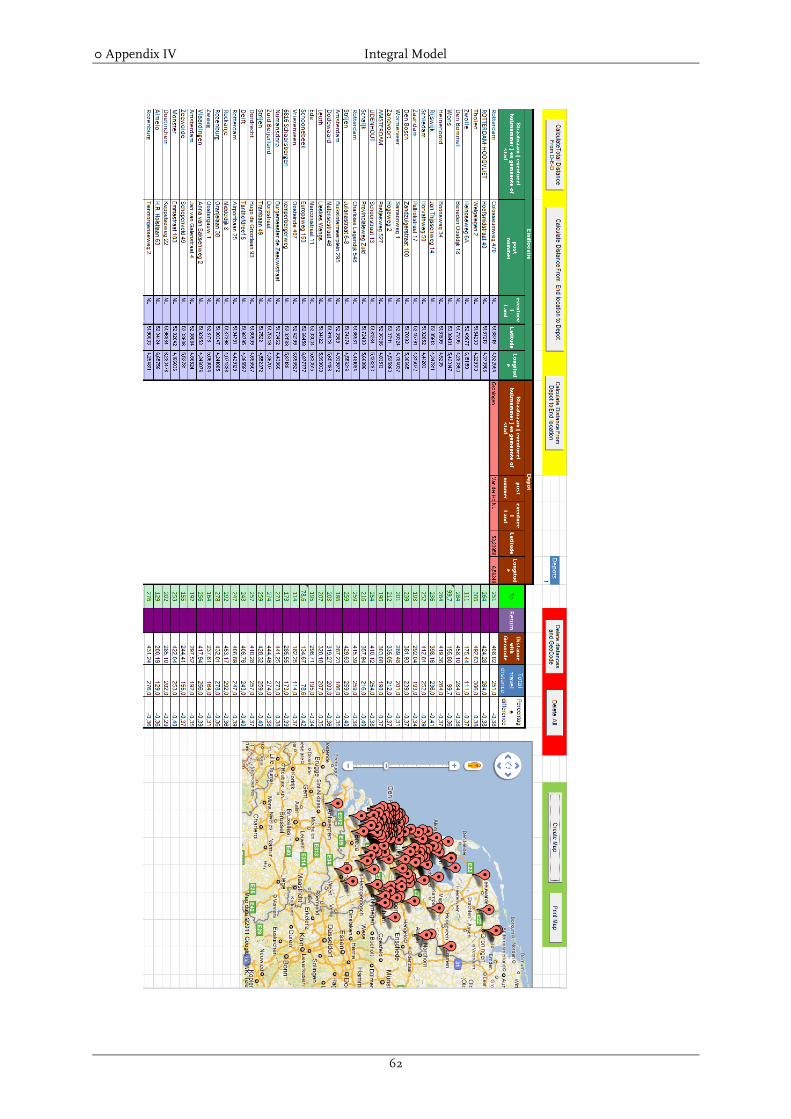
0 Appendix IV Integral Model
62

0 Appendix IV Integral Model
63

0 Appendix IV Integral Model
64