design and development of compact multiphoton … · date: 18 aug 2016 khanh q. kieu date: 18 aug...
TRANSCRIPT

DESIGN AND DEVELOPMENT OF COMPACT MULTIPHOTONMICROSCOPES
by
SeyedSoroush Mehravar
Copyright c© SeyedSoroush Mehravar 2016
A Dissertation Submitted to the Faculty of the
COLLEGE OF OPTICAL SCIENCES
In Partial Fulfillment of the RequirementsFor the Degree of
DOCTOR OF PHILOSOPHY
In the Graduate College
THE UNIVERSITY OF ARIZONA
2016

2
THE UNIVERSITY OF ARIZONAGRADUATE COLLEGE
As members of the Dissertation Committee, we certify that we have read thedissertation prepared by SeyedSoroush Mehravarentitled Design and Development of Compact Multiphoton Microscopesand recommend that it be accepted as fulfilling the dissertation requirement forthe Degree of Doctor of Philosophy.
Date: 18 Aug 2016Khanh Q. Kieu
Date: 18 Aug 2016Nasser Peyghambarian
Date: 18 Aug 2016Gholam A. Peyman
Date: 18 Aug 2016
Date: 18 Aug 2016
Final approval and acceptance of this dissertation is contingent upon the candi-date’s submission of the final copies of the dissertation to the Graduate College.I hereby certify that I have read this dissertation prepared under my directionand recommend that it be accepted as fulfilling the dissertation requirement.
Date: 18 Aug 2016Dissertation Director: Khanh Q. Kieu

3
STATEMENT BY AUTHOR
This dissertation has been submitted in partial fulfillment of the requirements
for an advanced degree at the University of Arizona and is deposited in the
University Library to be made available to borrowers under rules of the Library.
Brief quotations from this dissertation are allowable without special per-
mission, provided that an accurate acknowledgement of the source is made.
Requests for permission for extended quotation from or reproduction of this
manuscript in whole or in part may be granted by the head of the major de-
partment or the Dean of the Graduate College when in his or her judgment the
proposed use of the material is in the interests of scholarship. In all other in-
stances, however, permission must be obtained from the author
SIGNED: SeyedSoroush Mehravar

4
ACKNOWLEDGMENTS
Throughout my journey as a graduate student in College of Optical Sciences, I
received invaluable support from my family, advisors, colleagues and friends.
No need to say that without them, I would not have accomplished this much. I
would like to express my sincere gratitude here.
First and foremost, I would like to thank my advisor, Professor Khanh Kieu.
His passion about science and fundamental research has been a motivation for
me to work hard and try to implement the applied ideas through experiments.
Khanh discussed and debated all the ideas in my research studies, helped me
developing them, carefully read and edited numerous manuscript drafts, and
gave me a wealth of suggestions to improve. It was a great opportunity to work
closely with him and be part of his research team. I will never forget his efforts
to make me enthusiastic about the world and improving the lives using novel
scientific techniques. I have learnt from him a lot and I have rarely seen someone
like him to work hard with such enthusiasm and passion. I want to thank him
again for his patience and support.
Next, I have to sincerely appreciate my advisor and supervisor, Professor
Nasser Peyghambarian, who gave me the opportunity of being part of his team.
His support through these five years financially and emotionally helped me pur-
sue my studies and research. Without his effort to support the graduate students
by providing state-of-the-art equipment and laboratories, the research projects
would not have been completed.
Much gratitude goes to Dr. Gholam A. Peyman as my advisor and committee
member. He was a great mentor to me throughout the years we have been col-
laborating. His enthusiasm and passion about the research and making the lives
better is inexpressible. Besides his humbleness and kindness, his passion for sci-
ences makes him as my role model. He was the only individual that I could talk
about everything with him. I would like to thank Professor Masud Mansuripur,

5
who has been guiding me through these years. He was the very first person in
the College that I could stop by his office anytime and start a discussion. His per-
sonality and character is exemplary. I would like also to thank Professor Robert
A. Norwood, who was a great mentor for my projects. He has been always nice
to everyone and tried his best to solve students’ problems with his happy face
and unforgettable laughs.
Great faculty members and staff of the College of Optical Sciences have made
the past five years a unique experience for me. Majid Behabadi has been the only
person in the College always saying "Good Morning!" even at 5p.m. I would
like to thank him for his support and making our environment friendly and en-
joyable. The numerous support from Linda Schadler is greatly appreciated from
writing admission letters to providing funding sources for me. Mark Rodriguez
has helped me a lot as a graduate advisor throughout past three years. Amanda
Ferraris has been always there with her office door open when I’ve had questions.
Thank to Ruth Corcoran and Melissa Ayala for their great job and help. I should
also thank Palash Gangopadhyay for his support and being there whenever I had
scientific questions.
Special thanks to the former and current lab members and colleagues, Babak
Amirsolaimani, Soha Namnabat, Farhad Akhoundi, Dmitriy Churin, Roopa
Gowda, Raj Patil, Benjamin Cromey, Dawson Baker, Neil Ou, Jashua Olson, Erfan
Motefakker Fard, Sander Zandbergen, Roland Himmelhuber, Byron Coccolivo,
Lasse Karvonen, Antii Saynatjoki, Sasan and Nam Nguyen. I do believe that we
have made history to be remembered, both inside and outside the lab.
Additional thanks to my friends for being the ones that I always wanted,
needed, and appreciated. Negin, Kimia, Suzan, Mehrdad, Davoud, Andisheh,
Hameds, Nimas, Hamid and Elmira; Tucson will miss the time we spent together
after we leave. I would like to thank other close friends Arash, Soheil, Alireza
and Amirhossien, who although were not in Tuscon; they have been always in
my heart.
Last, but most importantly, my deepest debt of gratitude goes to my parents,

6
Ahmad and Effat, and my sweet little sister, Sepideh, for all their prayers, sup-
ports, and inspirations. I also would like to thank my best friends, Shiva, and my
wingman, Shayan, who have seen and helped me through every step I’ve taken
in the past few years. All my research projects have been supported by sate of
the Arizona TRIF Photonics and Imaging fundings.

7
DEDICATION
To my mother, father, and sister

8
TABLE OF CONTENTS
LIST OF FIGURES . . . . . . . . . . . . . . . . . . . . . . . . . . . . . . . . . . 10
ABSTRACT . . . . . . . . . . . . . . . . . . . . . . . . . . . . . . . . . . . . . 17
CHAPTER 1 Introduction . . . . . . . . . . . . . . . . . . . . . . . . . . . . 18
CHAPTER 2 Multiphoton Microscopy . . . . . . . . . . . . . . . . . . . . . 242.1 Multi-photon theory and instrumentation . . . . . . . . . . . . . . . 24
2.1.1 Theory . . . . . . . . . . . . . . . . . . . . . . . . . . . . . . . 242.1.2 MPM schematic . . . . . . . . . . . . . . . . . . . . . . . . . . 27
2.2 Optical Design . . . . . . . . . . . . . . . . . . . . . . . . . . . . . . . 302.2.1 Tube lens . . . . . . . . . . . . . . . . . . . . . . . . . . . . . . 322.2.2 Scan lens . . . . . . . . . . . . . . . . . . . . . . . . . . . . . . 342.2.3 Relay lens . . . . . . . . . . . . . . . . . . . . . . . . . . . . . 372.2.4 Entire optical design . . . . . . . . . . . . . . . . . . . . . . . 37
2.3 MPM characterization . . . . . . . . . . . . . . . . . . . . . . . . . . 412.3.1 Lateral and axial resolution using FL microspheres . . . . . 452.3.2 Measurement of lateral and axial resolution using nonlin-
ear knife edge technique . . . . . . . . . . . . . . . . . . . . . 462.3.3 Field curvature . . . . . . . . . . . . . . . . . . . . . . . . . . 51
2.4 Detection . . . . . . . . . . . . . . . . . . . . . . . . . . . . . . . . . . 54
CHAPTER 3 MPLAB: LabVIEW based laser-scanning software for multi-photon microscopy . . . . . . . . . . . . . . . . . . . . . . . . . . . . . . . 573.1 Data acquisition with NI-PCI-6110 using AI and AO ports . . . . . 573.2 Image analysis . . . . . . . . . . . . . . . . . . . . . . . . . . . . . . . 643.3 Challenges . . . . . . . . . . . . . . . . . . . . . . . . . . . . . . . . . 65
CHAPTER 4 Applications of MPM in bioscience and material characteriza-tion . . . . . . . . . . . . . . . . . . . . . . . . . . . . . . . . . . . . . . . . 694.1 Label-free multiphoton imaging of dysplasia in Barrett’s esophagus 69
4.1.1 Introduction . . . . . . . . . . . . . . . . . . . . . . . . . . . . 694.1.2 Multi-Photon Microscopy System . . . . . . . . . . . . . . . 714.1.3 Methods and Sample Preparation . . . . . . . . . . . . . . . 734.1.4 Results . . . . . . . . . . . . . . . . . . . . . . . . . . . . . . . 744.1.5 Discussion . . . . . . . . . . . . . . . . . . . . . . . . . . . . . 794.1.6 Conclusion . . . . . . . . . . . . . . . . . . . . . . . . . . . . 81
4.2 Multiphoton microscopy as a detection tool for photobleaching ofEO . . . . . . . . . . . . . . . . . . . . . . . . . . . . . . . . . . . . . . 81

TABLE OF CONTENTS – Continued
9
4.2.1 Introduction . . . . . . . . . . . . . . . . . . . . . . . . . . . . 814.2.2 Experimental setup . . . . . . . . . . . . . . . . . . . . . . . . 834.2.3 Results and discussion . . . . . . . . . . . . . . . . . . . . . . 854.2.4 Conclusion . . . . . . . . . . . . . . . . . . . . . . . . . . . . 91
4.3 Multi-photon microscopy for characterization of 2D materials . . . 92
CHAPTER 5 Summary . . . . . . . . . . . . . . . . . . . . . . . . . . . . . . 104

10
LIST OF FIGURES
1.1 a) Comparison between different imaging modalities in terms ofpenetration depth and resolution. b) Excitation volume for CWand femtosecond laser. In excitation with femtosecond laser onlythe focal volume of the objective lens is excited and photodamageand photobleaching are reduced for out-of-focus regions. . . . . . . 19
2.1 Jablonski diagram showing 5 different nonlinear process of 2PEF,3PEF, SHG, THG and CARS . . . . . . . . . . . . . . . . . . . . . . . 24
2.2 THG signal from center of a sphere with different sizes. The graphshows the FTHG and BTHG versus the sphere size and as can beseen the BTHG has smaller period compared to FTHG signal . . . . 28
2.3 SOLIDWORKS model of the MPM (courtesy of Benjamin Cromey) 282.4 Design of the first microscope prototype: schematic and spot dia-
gram for 1040nm illumination . . . . . . . . . . . . . . . . . . . . . . 312.5 OPD fan and field curvature for the first prototype design . . . . . 322.6 Simple objective lens representation . . . . . . . . . . . . . . . . . . 332.7 Tube lens schematic and the spot diagram for maximum 2.6 degree
optical FOV . . . . . . . . . . . . . . . . . . . . . . . . . . . . . . . . 342.8 OPD fan and field curvature of the tube lens . . . . . . . . . . . . . 352.9 Scan lens schematic and the spot diagram for 10 optical degree
scanning . . . . . . . . . . . . . . . . . . . . . . . . . . . . . . . . . . 362.10 OPD fan and field curvature of the designed scan lens for maxi-
mum 10 optical degree scanning . . . . . . . . . . . . . . . . . . . . 362.11 Relay lens system consisting of two achromatic lenses with 60mm
focal length and two meniscuses with 150mm focal lengths . . . . . 382.12 Entire imaging system shown for 10 optical degree scanning angle
and a paraxial objective lens model . . . . . . . . . . . . . . . . . . . 392.13 Spot and OPD fan diagrams. Note that for 10 optical degree scan-
ning angle, the FOV is 488µm× 488µm and almost diffraction lim-ited. The OPD fan shows a maximum aberration of 0.4 waves . . . 40
2.14 Field curvature and f-theta diagrams. The RMS wavefront error vs.field also shows that for optical fields below 8 degrees, the systemis diffraction limited . . . . . . . . . . . . . . . . . . . . . . . . . . . 40

LIST OF FIGURES – Continued
11
2.15 (a) Schematic of the MPM used for optical characterization of thesystem. MLL: Mode-locked laser, C: Collimator, G: Galvo scan-ners, SL: Scan lens, TL: Tube lens, D: Dichroic mirror, L: Lens, F:bandpass filter, PMT: Photomultiplier tube. (b) Emission spectrumof GaAs using 1040nm excitation wavelength. The power depen-dency measurements show the two and three photon process indi-cated by the slopes of 2 and 3, respectively . . . . . . . . . . . . . . 43
2.16 Two and three photon images of 0.5µm microspheres. The mea-sured data points are fitted with a Gaussian PSF and the FWHM ofthe PSF is considered as system resolution . . . . . . . . . . . . . . . 45
2.17 Resolution measurement using GaAs wafer. The laser scans acrossthe sharp edge of a GaAs wafer and the two and three photon pro-cess resolution is extracted by the curves fitted to the measureddata points . . . . . . . . . . . . . . . . . . . . . . . . . . . . . . . . . 47
2.18 Left: Schematic diagram of the objective lens field curvature (Pet-zval surface). Right: THG signal generated from the surface of theGaAs wafer when its location is below (down), at the focal plane(middle) and above (up) the focal plane . . . . . . . . . . . . . . . . 52
2.19 Top row: Objective lenses field curvatures for 20× aspheric (Left),40× Olympus (Middle) and 50× Jena Zeiss (Right). Bottomrow: projected Petzval surfaces in top row onto xz- and yz-plane.The projected curves are fitted by a quadratic curve showing thequadratic field dependency of field curvature . . . . . . . . . . . . . 53
2.20 Uncorrected cover slip (left) and corrected for field curvature im-age (right) using the data retrieved by measuring the field curva-ture for 20× aspheric objective lens . . . . . . . . . . . . . . . . . . . 54
2.21 Hamamatsu PMT data sheet and specifications . . . . . . . . . . . . 552.22 Box for controlling the gain of PMTs. A potentiometer controls the
gain voltage through a divider circuit. A LED indicates the on andoff status . . . . . . . . . . . . . . . . . . . . . . . . . . . . . . . . . . 56
3.1 MPLab control panel for image display and acquisition parameters 603.2 MPLab block diagram for writing and reading the data points . . . 613.3 nonuniform illumination correction. Left and right columns show
2PEFL and THG images before and after nonuniform illuminationcorrection. Scale bars: 600µm . . . . . . . . . . . . . . . . . . . . . . 66

LIST OF FIGURES – Continued
12
4.1 Schematic diagram of the in-house MPM system (left) and the mul-tiphoton spectrum of Barrett Esophagus tissue (right). Red: Opti-cal spectrum of the multiphoton generated signal from a normaltissue showing a strong THG signal at 520nm. Inset: zoom-inSHG spectrum . . . . . . . . . . . . . . . . . . . . . . . . . . . . . . . 72
4.2 Comparison between multi-photon microscopy and conventionallight microscopy of BE tissue that is negative for dysplasia. (a)H&E conventional light microscopy image showing intestinalmetaplasia with goblet cells. There is surface maturation, low nu-cle nuclear to cytoplasmic ratio and no dysplasia. (b-d) magnifiedregions shown in (a). (e) High resolution THG signal from MPMand (f-h) the magnified regions in (e). (i) SHG signal recorded si-multaneously with the THG signal showing collagen distributionin the stroma and blood vessels. (j-l) magnified marked regions inthe SHG image to show collagen in the basement membrane. TheTHG signal has a clear correlation to the H&E light-microscope im-age. The architectural structure of nuclei indicates that the tissuehas no dysplastic feature. The yellow arrows show the cells withno evidence of dysplasia. (FOV in (e) and (i): 1000× 750µm2, ac-quisition time: 2min) . . . . . . . . . . . . . . . . . . . . . . . . . . . 76
4.3 Multi-photon and conventional light microscopy images for low-grade dysplastic BE tissue. (a) Conventional light microscopy im-age of the tissue stained with H&E; there is intestinal metaplasiawith goblet cells, surface luminal cells displaying nuclear stratifi-cation, hyperchromasia, and an increased nuclear to cytoplasmicratio (N: C). (b-d) magnified regions marked in the H&E image.(e-h) High resolution THG images that show features of low-gradedysplasia in the same biopsy. (i-l) corresponding simultaneousSHG signals of the THG images that display the presence of col-lagen. The spatial distribution of cell nuclei is consistent with low-grade dysplasia. The cells with low-grade dysplasia are markedwith arrows. (FOV in (e) and (i): 750× 1000µm2, acquisition time:2min). The vertical white lines in (j)-(l) are the PMT artifacts . . . . 77

LIST OF FIGURES – Continued
13
4.4 MPM and conventional light microscopy images of high-gradedysplastic tissue. (a) Conventional light microscopy image of thetissue after labeling with H&E. There is a progressive dysplas-tic change in a background of intestinal metaplasia. Cells havemarked hyperchromatic nuclei nuclear stratification, loss of polar-ity and a markedly increased N:C ratio, considerably more thanin low grade dysplasia. (b-d) magnified squared regions markedin (a). (e) High resolution THG and (f-h) corresponding magni-fied regions. (i) High resolution SHG image and (j-l) the magni-fied regions marked in to show basement membrane collagen (i).The dense nuclei with variable shapes and sizes as well as the lossof orderly arrangement of the cells are consistent with high-gradedysplasia. Arrows represent the cells with high-grade dysplasia.(FOV in (e) and (i): 500× 500µm2, acquisition time: <1min) . . . . . 78
4.5 SHG signal from Barrett’s with non-dysplastic dysplasia (a), lowgrade dysplasia (b) and high grade dysplasia (c). Correspondinggraphs to the right show the thickness of the basement membranecollagen measured at each of the three chosen points per image,which confirm increasing thickness with progression of dysplasia . 80
4.6 The schematic of the multi-photon microscope, and b) diagramshowing various sources and probes on materials photodegrada-tion study . . . . . . . . . . . . . . . . . . . . . . . . . . . . . . . . . 84
4.7 LiNbO3 multiphoton spectrum excited at 1550nm, and b) normal-ized SHG intensity versus laser exposure timing for various laserpowers . . . . . . . . . . . . . . . . . . . . . . . . . . . . . . . . . . . 86
4.8 Multiphoton spectrum of DR1 on fused silica, the inset shows thelog-log plot of the output THG signal versus input power, b) nor-malized THG intensity versus exposure timing for various laserpowers, and c) THG profile of the sample where each square . . . . 87
4.9 DR1 decay curve with 30mW power (circle-marked line), best fit-ted one- (dash- dotted line), double-(dotted line), and stretched-exponential (solid line) functions, b) log- log plots of the photo-bleaching rates k1 and k2 vs. irradiation power, and c) the ratiobetween parameters k1 and k2 (left axis) and A1 and A2 (right axis)vs irradiation power . . . . . . . . . . . . . . . . . . . . . . . . . . . 88

LIST OF FIGURES – Continued
14
4.10 Multiphoton spectrum of SEO250 on fused silica, the inset shows aUV/Vis absorption spectrum of SEO250 (top) and the log-log plotof the output THG signal versus input power (bottom), b) normal-ized THG intensity versus laser exposure timing for various laserpowers, and c) THG profile of the sample where each square is con-tinuously exposed by a different laser power and exposure timing . 90
4.11 a) Fitting SEO250 decay curve with 19.8 mW power (circle-markedline) with 1- (dash-dotted line), 2-(dotted line), and stretched-(solidline) exponential functions. b) log- log plots of the photobleachingrates k1 and k2 for SEO250, inset: the ratio between parameters A1and A2 vs irradiation power, and c) the photobleaching rate versusirradiation power when the experimental data was fitted with astretched-exponential function . . . . . . . . . . . . . . . . . . . . . 91
4.12 (a) Composite of SHG (red) and THG (green), (b) SHG in the poledregion, (c) THG from on top of the gold electrodes. The orange boxin (b) indicates the region in which the quantitative SHG data wascollected. (d) Ratio of the measured r33 to the square root . . . . . . 93
4.13 Typical multiphoton micrographs of a sample containing exfoli-ated graphene on SiO2/Si substrate. (a) Fluorescence, (b) third-harmonic signal, and (c) merged RGB image using fluorescence(red) and THG (green) signals. One particularly interesting few-layer graphene flake considered below is marked with white cir-cles and shown magnified in the merged RGB image . . . . . . . . 93
4.14 Dependence of the THG peak signal on the laser peak power andnumber of graphene layers. Dots are measurement values; thecurves are exponential fits to the power dependence. In the log-arithmic plot in the inset, three points corresponding to the low-est THG power deviate from the general trend because the powerlevel is below the linear regime of our detection system . . . . . . . 95
4.15 (a) SHG and (b) THG images of the few-layer GaSe flake, (c) RGBcomposite image generated from the SHG and THG images, and(d) cross-sections of the SHG and THG signals taken from thewhite dashed line in (c). The spectra of the generated light havebeen measured from the points marked with Roman numbers II,V and VII in (c). (e). Measured spectra of the generated light fromthree different positions (different thicknesses) on the flake. Thepositions are marked by Roman numbers II, V and VII . . . . . . . 96

LIST OF FIGURES – Continued
15
4.16 Power dependence of the (a) SHG and (b) THG signals. (c) SHGand THG signals as a function of the number of the GaSe layersmeasured with 1kW excitation peak power . . . . . . . . . . . . . . 97
4.17 (a) SHG and (b) THG images of the few-layer GaTe flake. (c) RGBcomposite image generated from the SHG and THG images. (d)Cross-sectional SHG and THG signals taken from the blue dashedline in (c); scale bars in the SHG and THG images are 10µm. (e)AFM image of the staircase area where the intensity is at maximumfor both SHG and THG. (f) AFM cross-section of the staircase areataken from the white dashed line B-B’ in (e) showing the steps from17 to 57nm. Excitation peak power dependence of the (h) SHG and(i) THG signals. The lines are fits to square (h) and cubic (i) powerdependences . . . . . . . . . . . . . . . . . . . . . . . . . . . . . . . . 98
4.18 SHG intensity versus the induce voltage across the electrodes . . . 994.19 Normalized multiphoton excitation spectra and micrographs of (a)
the blend of BBCP D with 30 wt % QDs and (b) neat polymer sam-ple. The wavelength of light for excitation was 1550nm . . . . . . . 100
4.20 Damage threshold of directly deposited graphene is comparableto mono- and bi-layered graphene prepared by the transfer tech-nique. ÎTIntensity is the intensity difference of THG signal be-tween the studied area and the reference area. The damage areahas less THG than the pristine area. Multiphoton microscopic im-ages of (a) transferred graphene film with a tear and folded ar-eas and (b) directly deposited graphene with a scratch made by ascalpel. (a-inset) average graphene film thickness is comparable tofolded bi-layered graphene prepared by transfer technique. (Bothimage size is about 300× 300µm2. Color bar indicates the intensityof THG signal.) . . . . . . . . . . . . . . . . . . . . . . . . . . . . . . 101
4.21 (a) Optical setup used to measure the third-harmonic signal of thesilicon samples. (b) Measured third-harmonic spectra for the sam-ples with different trench and ridge geometries. (c) THG signal asa function of the angle of polarization of the input be beam. (d)Spatially resolved optical images of the third-harmonic signal fortwo orthogonal polarizations of the input beam . . . . . . . . . . . 102
4.22 Multiphoton microscope images of the boundaries between tex-tured (left) and planar (right) substrates coated with rhodamine6G (a), green fluorescent protein (b), and chlorophyll (c) . . . . . . . 103

LIST OF FIGURES – Continued
16
4.23 Fluorescence signals (left column) and enhancements (right col-umn) calculated from the MPM measurements. The inset showsfive images of the R6G sample at different focus positions . . . . . . 103

17
ABSTRACT
A compact multi-photon microscope (MPM) was designed and developed with
the use of low-cost mode-locked fiber lasers operating at 1040nm and 1560nm.
The MPM was assembled in-house and the system aberration was investigated
using the optical design software: Zemax. A novel characterization methodology
based on ’nonlinear knife-edge’ technique was also introduced to measure the
axial, lateral resolution, and the field curvature of the multi-photon microscope’s
image plane. The field curvature was then post-corrected using data processing
in MATLAB. A customized laser scanning software based on LabVIEW was de-
veloped for data acquisition, image display and controlling peripheral electron-
ics. Finally, different modalities of multi-photon excitation such as second- and
third harmonic generation, two- and three-photon fluorescence were utilized to
study a wide variety of samples from cancerous cells to 2D-layered materials.

18
CHAPTER 1
Introduction
Multi-Photon Microscopy (MPM) is a nonlinear imaging modality that provides
sub-micro meter resolution images with millimeter penetration depth. The use of
high peak power laser pulses generates a tremendous photon flux confined at the
focal volume of a high numerical aperture (NA) objective lens resulting is an op-
tical sectioning enabling 3D reconstruction of highly scattering tissues. There are
various imaging modalities with different working principals and applications.
In each technique there is a trade-off between penetration depth and resolution of
the imaging. Figure 1.1(a) illustrates this trade-off pictorially for different imag-
ing modalities. Among them, MPM can provide sub-micrometer resolution with
descent penetration depth of ∼ 2mm. The inherent optical sectioning property of
MPM which confines the excitation only in the small focal volume of an objective
lens reduces the out-of-focus photobleaching and photodamage significantly, the
known issues with continuous-wave (CW) excitation (Figure 1.1(b)).
Two-photon absorption was first predicted by Maria-Goeppert-Mayer (1906-
1972) in her doctoral dissertation in 1931, but it was only back in 1992 that Denk,
Strickler and Webb developed the idea of combining two-photon absorption with
laser scanning technique to create high-resolution images [1] . MPM has shown
its potential for a wide range of applications in neuroscience, cancer detection
and high-resolution 3D writing. There are different imaging modalities such as
Two- and Three-Photon Excitation Fluorescence (2PEF, 3PEF), Second- and Third-
Harmonic Generation (SHG, THG) in Multi-Photon Imaging (MPI) providing dif-
ferent and complementary information about the sample under test. 2PEF and
3PEF signals are generated when atom or molecule transits from ground state to

19
Figure 1.1: a) Comparison between different imaging modalities in terms of pene-tration depth and resolution. b) Excitation volume for CW and femtosecond laser.In excitation with femtosecond laser only the focal volume of the objective lensis excited and photodamage and photobleaching are reduced for out-of-focus re-gions.
the excited state which in turn emits a light at a wavelength normally in the vis-
ible range of light. SHG and THG are coherent signals that a photon at exactly
half and 1/3 of the excitation wavelength is generated when two or three pho-
tons are scattered by tissue simultaneously. The harmonic signal is directional
and depends on the distribution and direction of the induced dipoles in the fo-
cal plane of the sample. SHG can be found in samples where centro-symmetry
is broken such as collagen and fibrous structures in biological specimen. THG is
sensitive to the interfaces and can be generated where refractive index changes. It
was shown that THG signal can be used to distinguish cell boundaries and struc-
tures for label-free imaging of different stages of dysplasia in Barrett’s esopha-
gus [2] and imaging of targeted lipid microbubbles for cancer studies [3]. THG
was also used to monitor the photobleaching of electro-optical polymers under
femtosecond illumination [4]. Two-photon microscopy was also used in neuro-
science for brain studies [5], dynamic calcium monitoring [6]. Horton et.al [7]

20
used 1700nm excitation wavelength to generate THG and 3PEF signals for in
vivo studies of mouse brain and achieved 1.6mm penetration depth inside the
cortex. Another suitable wavelength for brain studies was proved to be 1060nm
using low-cost and compact fiber lasers with low repetition rates [8, 9, 10]. An
automated method by combining two-photon fluorescence microscopy and tis-
sue sectioning used to reconstruct mouse brain in 3D [11]. Mahou et.al used
femtosecond Ti:Sa laser followed by OPO to simultaneously excite three chro-
mophores generating multi-color two-photon imaging by wavelength mixing
[12]. Custom-made MPM were reported in literature for ex-vivo and in-vivo
studies. Negrean et.al optimized the scan and tube lens design for two-photon
microscopy covering 600-1700nm wavelength region [13]. Large field of view
(FOV) MPM were also designed achieving 5mm FOV to study murine cortex [14].
Another approach was demonstrated by Stirman et.al for two-photon calcium
imaging with > 9.5mm2 FOV [15]. Parabolic mirrors were used to improve the
laser scanning in confocal and two-photon microscopy [16, 17]. A cost-effective
and high-performance two-photon microscope was reported in [18] explaining
the system design and modification for different applications. A custom-made
two-photon microscope was also developed for video-rate Ca2+ imaging [19].
Nikolenco et.al converted a confocal microscope scan head to two-photon micro-
scope for brain imaging [20]. Random pattern scanning technique was utilized
for fast 3D imaging of dendrite processes [21], dendrite Ca2+ spike propagation
[22] and cellular network dynamics [23]. Flusberg et.al designed and fabricated
an ultra-light weight microendoscope for in vivo brain imaging [24]. MPM re-
quires a mode-locked laser to provide high peak power pulses for initiating non-
linear interaction while preserving low average power to avoid thermal damage
on tissue. Ti:Sa lasers are still the workhorse of the MPI field covering excitation
wavelengths from 700nm to 1100nm [25, 26, 27, 28, 29, 30, 31, 32, 33]. Squier and
Miller reviewed the laser sources for high resolution nonlinear microscopy [34].

21
The first demonstration of laser scanning microscopy by using Ti:Sa mode-locked
laser backs to 1992 [35]. However, the cost and size of Ti:Sa laser prevent MPM to
be used widespread in clinical application. Moreover, it requires frequent align-
ment for long-term operation. Based on scattering theory, utilizing longer NIR
wavelength results in deeper penetration inside the scattering tissue. Therefore,
there is a need to develop compact and low-cost fiber based mode-locked laser
to address the current issues with the excitation source. There has been a strong
research and development on using fiber lasers in the field of MPI [36, 37]. A com-
prehensive review on the fiber laser source development for MPM was reported
by Xu and Wise in [38]. There are three major wavelength regions for designing
mode-locked fiber lasers. Yb3+ [39, 40, 41], Er3+ and Tm3+ doped fibers cover
1020-1100nm, 1520-1630nm and 1850-2000nm wavelength regions, respectively.
However, new windows are being investigated that can cover 1300nm wave-
length where biological tissues have low water absorption. Currently, semicon-
ductor saturable absorber mirrors (SESAM) and nonlinear polarization evolution
(NPE) are the key important elements to achieve passive mode-locking in fiber
lasers [33, 42, 43]. There are limitations in performance and stabilities of mode-
locked lasers based on SESAM and NPE. Carbon nanotube saturable absorber
(CNTSA) [44, 45] seems to be a promising replacement for passive mode-locking
providing compact, low-cost and stable performance design [46]. Adaptive op-
tics was utilized to modify the beam wavefront to generate almost aberration-free
waveform resulting in sharp images at deep penetration inside a tissue [47, 48].
Neil et.al used a spatial light modulator to correct specimen-induced aberration
in two-photon and confocal microscopy [49]. The parameters estimating the ac-
curacy of sensorless adaptive optics was investigated theoretically and experi-
mentally in [50]. The wavefront correction can be done in real-time for in vivo
applications [51, 52, 53]. In adaptive optics, a deformable mirror is used to ma-
nipulate the initial wavefront and compensate for the known wavefront aberra-

22
tion existed in the two- or multi-photon microscopy system [54, 55, 56]. Different
implementations and techniques have been reported to use adaptive optics in
two-photon microscopy [57, 58]. Finally, the performance of sensorless adaptive
optics for multiphoton microscopy was reported in [59] and two, three and four
photon microscopy were compared in [60]. MPM is a raster scanning imaging
modality in which the limited power of the laser source makes fast imaging of
structures in 3D challenging. There are different techniques to fasten the image
acquisition up to video rate in MPM. One technique called "multifocal multipho-
ton microscopy (MMM)" is based on the incident beam distribution over multiple
foci [61, 62, 63, 64, 65, 66, 67]. Then the frame rate scales with the number of exci-
tation foci. One of challenges with MMM is the constructive interference between
multiple foci resulting in a decrease in axial resolution. However, this issue can
be solved by delaying the successive foci in time. A frame rate of 600Hz was
reported by Bahlmann et.al using this implementation [61]. In MMM a single el-
ement detector can no longer be used since different foci have to be mapped into
a 2D plane detector. However, this limitation can be solved by using segmented
detector or descanned detection scheme. Kim et.al followed this approach by us-
ing multianode PMT in which each anode receives photons from corresponding
foci on the sample [68]. Another approach for video rate MPI is to use poly-
gon [69] or resonant scanners [19, 70, 71]. In this technique the repetition rate
of the excitation source has to be designed so that there are enough pulses per
pixel dwell time required for excitation. Since using polygon and resonant scan-
ners do not have flexibility to scan a region of interest with arbitrary scan field,
acousto-optic deflectors and tunable lenses are used to address this issue. Using
acousto-optic deflectors researchers can access to multiple regions of interest at
different lateral planes [72, 73, 74, 75, 76, 77, 78, 79, 80]. Spatiotemporal focusing
can also increase the imaging rate in which the pulse is stretched in wavelength
using gratings or prisms and then coupled back only at the focal plane of the ob-

23
jective lens [81, 82, 83, 84, 85, 86, 87, 88, 89]. Finally, a high speed imaging device
can be realized by rapid axial scanning of the beam instead of lateral scanning
by modifying the divergence of the beam at back aperture of the objective lens
(remote focusing) [90, 91, 92, 93, 94].

24
CHAPTER 2
Multiphoton Microscopy
2.1 Multi-photon theory and instrumentation
2.1.1 Theory
MPM is a nonlinear process in which multiple photons are nearly simultaneously
absorbed by the material and another photon with larger energy compared to the
excitation photon is generated. Figure 2.1 below shows different multi-photon
interaction processes. In 2PEF modality two photons are absorbed and the atom
or
Figure 2.1: Jablonski diagram showing 5 different nonlinear process of 2PEF,3PEF, SHG, THG and CARS
molecule transits from ground state to the excited state. Then, the atom or
molecule emits a photon to come back to the ground state. The same scenario

25
occurs for 3PEF. In harmonic generation process, two or three photon are scat-
tered simultaneously, but the transition occurs between the ground state and a
virtual state instead of a real state as happening in 2- and 3PEFL. Therefore, har-
monic generation is a parametric process in which the energy is preserved and
the emitted photon is coherent and has an energy exactly equal to the harmonic of
the excitation photon. Coherent Anti-Stoke Scattering (CARS) is another multi-
photon process which is sensitive to the vibration states of the molecules and can
be used to image chemical bonds. The efficiency of a nonlinear process depends
on different parameters. Nonlinear process occurs only when the incident pho-
tons are confined or concentrated in time and space simultaneously. The space
confinement can be fulfilled using high NA objective lenses. However, realiz-
ing confinement of photons in time is expensive and hard to implement. This
requires to use ultra-short mode-locked lasers and this type of excitation source
is the main cost of a MPM. The efficiency of multi-photon process scales with
( 1frτ )
n−1, in which n, fr and τ are the nonlinear order, laser repetition rate and
pulse duration. For example, for two-photon process the fluorescence signal can
be formulated as [95] :
FL =ησ
τ f 2r
(πNA2
hcλ
)2
〈P〉2e−2z/ls (2.1)
Where η, σ, h and c are the fluorophore quantum efficiency, fluorophore two-
photon absorption cross section, Planck’s constant and speed of light, respec-
tively. 〈P〉 is the laser average power and ls is the scattering length for the tissue
at the excitation wavelength. Note that, the average power has to be kept low
to avoid damage or photobleaching of the tissue. This requires to decrease the
laser repetition rate to generate large pulse energy. Due to the Mie scattering
theory, the scattering at longer wavelengths scales with λ−4, resulting in larger
penetration depth in a highly scattering material for NIR excitation wavelength
(assuming linear absorption is small). Moreover, the longer wavelength pho-

26
tons have smaller photon energies preventing damage on the samples. However,
the spot size increases at longer wavelengths resulting in decreased lateral and
axial resolution. In nonlinear harmonic generation processes, the induced polar-
ization from the intense incident electric fields generates new frequencies which
are not in the spectrum of the incident light. In harmonic generation processes
the energy is preserved while momentum conservation may not be required. In
the case where momentum is also conserved the wave coupling increases conse-
quently. The momentum conservation is known as phase matching which occurs
in nonlinear harmonic signals such as SHG and THG [96]. Nonlinear Schrödinger
equation is used to explain the coupling between the incident electric field and
the induced polarization which for THG process can be formulated as [97]:
∇2E(3ω) +n2(3ω)(3ω)2
c2 E(3ω) =(3ω)2
ε0c2 χ(3)(3ω, ω, ω, ω)E3(ω) (2.2)
In which the electric fields at the fundamental wavelength and THG are:
E(ω) ∝ A1ei(k1z−ωt) (2.3)
E(3ω) ∝ A3ei(k3z−3ωt) (2.4)
In which k1 = n(ω)ω/c is the wave number at fundamental frequency. Using
slowly-varying amplitude approximation (SVAA), the solution of the nonlinear
wave equation at z = l inside the sample can be expressed as:
E(3ω) ∝ A13lsinc(
∆kl2
) (2.5)
In which ∆k = k(3ω) − 3k(ω) = 3ω(n(3ω) − n(ω))/c is the wavenumber
mismatch resulting from the dispersion of the refractive index. When ∆k = 0
phase matching condition occurs; however, due to the dispersion of refractive
index phase matching does not usually occur. Therefore, the harmonic electric
field depends on the sample thickness and oscillates with the period of π/∆k

27
which is called the coherence length (lc). Considering the incident wave as a
plane wave, the forward and backward coherence length can be formulated as:
lFTHGc =
π
k(3ω)− 3k(ω)(2.6)
lBTHGc =
π
k(3ω) + 3k(ω)≈ λ
12n(ω)(2.7)
Considering negligible refractive index dispersion. This shows that backward
coherence length is smaller than the forward one. For a focused Gaussian wave
the forward coherence length can be described as [98]:
lFTHGc,gaus =
π
|k(3ω)− 3(k(ω) + kG|)≈ π
3|kG|(2.8)
Where kG is the Gouy phase shift and can be described as the phase difference
between the focusing beam and harmonic plane wave propagation along the op-
tics axis. For strong focusing beam this phase shift is dominant over the mate-
rial dispersion. Due to the sinc- shape electric field the forward THG (FTHG)
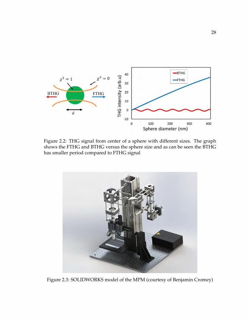
and backward THG (BTHG) signals have periodic behavior based on the size
of the sample, but BTHG has smaller period compared to FTHG signal. Figure
2.2 below compares the FTHG and BTHG signals for a sphere in a homogenous
medium.
Moreover, the influence of NA, dispersion, orientation and incident polariza-
tion can be found in [98].
2.1.2 MPM schematic
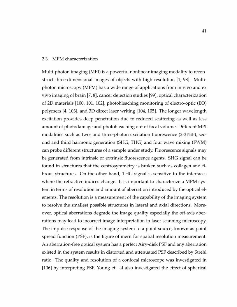
Figure 2.3 shows the schematic design of the MPM using SOLIDWORKS.
The fiber laser delivers the ultra-short pulses at 1550nm and 1040nm excita-
tion wavelengths to the galvo-galvo scanning system. A collimator designed at
the excitation wavelength from Thorlabs is used to collimate the laser beam be-
fore being deflected by the first galvo mirror (Y). A relay lens system is used to
28
Figure 2.2: THG signal from center of a sphere with different sizes. The graphshows the FTHG and BTHG versus the sphere size and as can be seen the BTHGhas smaller period compared to FTHG signal
Figure 2.3: SOLIDWORKS model of the MPM (courtesy of Benjamin Cromey)

29
image the laser beam from the Y-mirror surface to the surface of the second mir-
ror (X-mirror) in order to prevent vignetting in the image. Each element of the
relay lens has a focal length of 40mm. The relay lens system has a transmission of
90% using C-coated lenses. A telescope path consisting of scan and tube lenses
are used to expand the incident beam to fill the back aperture of the objective lens.
The magnification value is defined by ratio of the objective lens back aperture to
the collimator size which is here 4 times. Using compound lenses can realize the
maximum possible FOV that can be supported by the objective lens. The process
of selecting scan lenses and tube lenses are explained in detail in the following
sections. A dichroic mirror is used to separate the excitation wavelength from
the generated up-converted signal from the sample. The nonlinear multi-photon
processes occur at the focal volume of the objective lens where the high photon
flux initiates the nonlinear processes. This is why pulsed lasers with large peak
powers are typically used in nonlinear imaging. The objective lens has to have
good transmission both at the excitation wavelength and the up-converted sig-
nal which is normally in the visible region of light. This accompanying with the
aberration-corrected design make the objective lenses cost effective and an impor-
tant element in each MPM system. When sample is excited, the generated light
can be collected in forward and backward directions. The harmonic generated
signals have larger values in the forward direction due to the phase-matching
condition that can be collected using a condenser. However, the forward collec-
tion requires a thin slice of the sample and for thicker samples or in vivo appli-
cation the signal is collected in the backward direction. The backward generated
signal is then redirected to the detection unit using the pump/signal dichroic
and another dichroic to isolate different spectral regions corresponding to dif-
ferent imaging modalities. The selection of the second dichroic mirror and the
filters in front of the PMTs is based on the nature of the signal to be detected. For
example, for SHG and THG signals narrow band-pass filters are required, while

30
fluorescent signal needs filters with larger bandwidths. Due to the signal leakage
between the channels, it is possible to un-mix the signal using simple algorithms
providing that the contribution of each channel through the other one is already
known or can be measured. It might be possible to use CCDs for image recon-
struction and recording the pixel intensities; however, PMTs are better options
due to their sensitivities and their noise performance. The output of the PMTs
are then amplified using low-noise current amplifiers before being digitized by
an analog to digital (A/D) convertor (NI PCI 6110). The DAQ card has two ana-
log outputs to control the galvo-galvo mirrors and multiple analog inputs. The
data acquisition rate can be set up to 5MS/s per channel as mentioned in the PCI
data sheet. A customized LabVIEW program has been developed to acquire data
and construct the images. The data acquisition was synchronized with periph-
eral devices for 3D imaging. A motorized stage (LSI LXI 4000) is used to move
the sample in x, y and z directions. The resolution of the stage is ∼100nm based
on the data sheet. It can move 10cm laterally and 2cm axially.
2.2 Optical Design
In multi-photon imaging (MPI), it is important that image is reconstructed with
minimum amount of aberrations. The aberration can modify the image quality
resulting in incorrect interpretation which is vital for in vivo applications. The
aberration can be balanced through the optical modeling design using Zemax
software. In Zemax, the lenses are loaded into the software using the available
library and the distance between the optical elements are optimized using op-
timization function. The first design prototype includes two achromatic lenses
and the objective lens is assumed to be a paraxial surface, since there is typically
no information regarding to the optical design of the objective lens. There are
several conditions that needs attention to meet the best performance of the mi-

31
croscope. In order to utilize the full NA of the objective lens, its back aperture
has to be filled by expanding the incident beam diameter. In the first design,
we used a collimator (F280FC-980 and F280FC-1550, Thorlabs) with exit beam
diameter of 3.6 mm. The objective lenses we are using for our experiment have
13-15mm back aperture, therefore a magnification of 4 is required. There are
different sets of scan and tube lenses with the focal lengths ratio of 4 that can be
chosen. However, it is better to use the lenses with larger focal length due to the
reduced aspherical aberration. There are two drawbacks on selecting the larger
focal length lenses. First, the total length of the system is increased making the
system large. Second, since we are using 25.4mm (1inch) lenses, the optical angle
scanning range is reduced using a large focal length scan lens resulting in small
FOV. For the first design, I have chosen achromatic lenses with 40mm and 150mm
focal lengths (AC254-40-B and AC254-150-B, Thorlabs) as scan and tube lenses,
respectively. Figure 2.4 shows the Zemax layout and the optical elements.
Figure 2.4: Design of the first microscope prototype: schematic and spot diagramfor 1040nm illumination
The design was optimized for spot radius and the operating wavelength of
1040nm. The spot diagram was also shown in this figure. The OPD fan nd the
field curvature curves for this design are also shown in Figure 2.5.

32
Figure 2.5: OPD fan and field curvature for the first prototype design
This design suffers from astigmatism, distortion and field curvature aberra-
tions. The maximum field curvature and the astigmatism for tangential and sagit-
tal cross sections are 2.07 and 0.88 waves (Figure 2.5). The maximum HFOV by 7.5
optical degrees scanning of the mirrors is 500µm for an objective lens with 20×magnification and 10mm focal length (Nikon S Fluor, 0.75 NA). As can be seen in
Figure 2.4 the system is not diffraction limited for the optical field of larger than
5 degree. Note that, in this design the back aperture of the objective lens was not
filled out completely to realize maximum supported NA for the best resolution
performance. Considering these issues, I started to design a system using com-
pound lenses instead of single lenses as scan and tube lenses. Each compound
scan and tube lens was separately optimized to realize a tele-centric system. The
detail of the design will be explained in the following subsections.
2.2.1 Tube lens
Instead of starting with scan lens design, it is better to first design the tube lens
and based on the required field angle then design the scan lens. There are several
criterion that have to be met first to design a tube lens. One is the maximum
ray angle exiting the tube lens. This ray angle is defined by the objective lens

33
specifications. Figure 2.6 below shows a schematic of the ideal objective lens
and the parameters required to define the entrance ray angle to its back aperture.
I mainly focus on two objective lenses mostly used for our experiments. The
first one is Nikon 40× with 1.3NA oil immersion. This objective lens has a back
aperture of 13mm. The focal length of the objective lens can be calculated as:
Figure 2.6: Simple objective lens representation
NA = nf
2D(2.9)
Where n = 1.52 is the refractive index of oil. Then the focal length is calculated
to be f = 8.18mm. The maximum FOV is defined as the ratio of the field number
(assuming 20) and the magnification (40×) which is 0.5mm. The incident beam
angle is then:
2 f αin ≈ FOV ⇒ αin =FOV
2 f= 0.03rad = 1.75◦ (2.10)
This is the exit ray angle for the tube lens, as well. The entrance pupil in Zemax
for the tube lens design was also set to 13mm representing the back aperture size

34
of the objective lens. After examining different sets of scan and tube lenses with
the ratio of 4, I decided to use a tube lens with a focal length of 125mm. It is pos-
sible to use either a single achromatic doublet with a 125mm focal length or two
back-to-back 250mm focal length achromatic doublets. Using two doublets give
the software a few degrees of freedom to optimize the aberrations and realizing
the image-space telecentricity for the tube lens. Moreover, spherical aberration
is reduced 4 times using two achromatic lenses having 2f focal lengths instead of
using one doublet with a focal length of f. Figure 2.7 shows the optical layout and
the spot diagram using two doublets.
Figure 2.7: Tube lens schematic and the spot diagram for maximum 2.6 degreeoptical FOV
The incident wavelength was set to 1040nm and I used a Gaussian approxi-
mation with an apodization factor of 1. Figure 2.8 shows the OPD fan and field
curvature/astigmatism. Note that this is the inverted order of elements in the
layout, since the stop aperture was inserted at the first surface.
2.2.2 Scan lens
After designing a compound tub lens, a scan lens with a focal length of 30mm
is required to expand the incident beam by a factor of 4. It is possible to use

35
Figure 2.8: OPD fan and field curvature of the tube lens
commercial scan lenses from Thorlabs which are designed specifically for Opti-
cal Coherence Tomography (OCT) applications, but they are expensive and are
not normally designed for longer NIR wavelengths (i.e. 1550nm). Note that the
distance between the first surface of the compound scan lens and the scanning
mirror must be larger than 25mm which is the half size of the galvo mirror cage.
There are different approaches to designing a scan lens with 30mm focal length
and object telecentricity. One can use a single doublet, but by using a single lens
we are not able to control the telecentricity. Another approach is to use two back-
to-back 60mm focal length doublets followed by a meniscus. As mentioned above
using two doublets decreases the spherical aberration. Using meniscus reduced
the spherical aberration additionally and let us to control the focal length of the
compound lens. Figure 2.9 shows the optical layout of the compound scan lens.
In the optimization merit function, I used the operand "RANG" (ray angle) to
minimize the chief ray angle for different field angles. Moreover, the distance be-
tween the mirror, achromatic and meniscus lenses can be varied in order to reach
a 30mm focal length. The whole scan lens design then optimized using spot size
radius with 8 rings and 8 arms and maximum glass-air distance of 50mm.
The spot diagram of the compound lens was also shown in Figure 2.9. Figure

36
Figure 2.9: Scan lens schematic and the spot diagram for 10 optical degree scan-ning
2.10 illustrates the OPD fan and field curvature/astigmatism of the design. Back
to the tube lens design, the image surface size was calculated to be 6mm which
is the image size after the scan lens due to the inverted design of the tube lens.
Figure 2.10: OPD fan and field curvature of the designed scan lens for maximum10 optical degree scanning

37
2.2.3 Relay lens
In typical MPM a galvo-galvo mirror scanning system is used to realize laser
raster scanning for 2D image reconstruction. The distance between the mirrors
surfaces are typically 1cm. The laser beam is deflected from the surface of the
first galvo mirror (X-mirror) before reaching to the surface of the second galvo
mirror (Y-mirror). The distance between the first surface of the scan lens and
the galvo-galvo system is so that that the mid-distance between the galvo mir-
rors is considered as the entrance pupil of the scan lens. In an imaging system
the image of the laser source has to be imaged on the back aperture of the ob-
jective lens. However, the beam should not move laterally on the back aperture
but only pivoting around the center of the back aperture. When the galvo mir-
rors are close to each other, the image of the incident beam is displaced across
the back aperture. In order to fix this issue, a relay lens configuration is needed.
In a relay lens system, the incident beam is relayed (imaged) on the surface of
the second mirror after deflection from the first galvo mirror. Figure 2.11 shows
the optical layout of the relay lens system. In a relay system two identical com-
pound lenses are used to maintain a unit magnification as well. For this design, I
used an achromatic doublet followed by a meniscus as the relay lens compound
lens. This compound configuration was then optimized to make a tele-centric
lens system. After the relay lens system, it is important that the different field ray
angles should intersect at the same points along the optical axis to maintain the
best performance of the following scan and tube lens configuration.
2.2.4 Entire optical design
After optimal design of relay, scan and tube lenses, they are sequentially inserted
into Zemax lens data and the distances between the lenses are optimized again
considering the aberrations that have to be minimized. As mentioned above, a

38
Figure 2.11: Relay lens system consisting of two achromatic lenses with 60mmfocal length and two meniscuses with 150mm focal lengths
paraxial surface was used as an ideal objective lens. Figure 2.12 shows the entire
design of the optical path.
The spot diagram was also shown in Figure 2.13 indicating the good perfor-
mance of the system with the proposed design. Distortion has the largest contri-
bution to the aberration existed in the current design. The maximum aberration
in OPD fan is 0.4 waves.
The field curvature diagram (Figure 2.14) shows 2µm field curvature aberra-
tion. For scanning angles below 8 optical degrees the system is almost diffraction
limited. Note that, although the lenses used in this design are B-coated, this de-
sign has the same performance using 1550nm excitation source at the cost of a
slightly change in the focal plane due to the axial chromatic aberration and 50%
transmission loss.

39
Figure 2.12: Entire imaging system shown for 10 optical degree scanning angleand a paraxial objective lens model

40
Figure 2.13: Spot and OPD fan diagrams. Note that for 10 optical degree scanningangle, the FOV is 488µm× 488µm and almost diffraction limited. The OPD fanshows a maximum aberration of 0.4 waves
Figure 2.14: Field curvature and f-theta diagrams. The RMS wavefront error vs.field also shows that for optical fields below 8 degrees, the system is diffractionlimited
41
2.3 MPM characterization
Multi-photon imaging (MPI) is a powerful nonlinear imaging modality to recon-
struct three-dimensional images of objects with high resolution [1, 98]. Multi-
photon microscopy (MPM) has a wide range of applications from in vivo and ex
vivo imaging of brain [7, 8], cancer detection studies [99], optical characterization
of 2D materials [100, 101, 102], photobleaching monitoring of electro-optic (EO)
polymers [4, 103], and 3D direct laser writing [104, 105]. The longer wavelength
excitation provides deep penetration due to reduced scattering as well as less
amount of photodamage and photobleaching out of focal volume. Different MPI
modalities such as two- and three-photon excitation fluorescence (2-3PEF), sec-
ond and third harmonic generation (SHG, THG) and four wave mixing (FWM)
can probe different structures of a sample under study. Fluorescence signals may
be generated from intrinsic or extrinsic fluorescence agents. SHG signal can be
found in structures that the centrosymmetry is broken such as collagen and fi-
brous structures. On the other hand, THG signal is sensitive to the interfaces
where the refractive indices change. It is important to characterize a MPM sys-
tem in terms of resolution and amount of aberration introduced by the optical el-
ements. The resolution is a measurement of the capability of the imaging system
to resolve the smallest possible structures in lateral and axial directions. More-
over, optical aberrations degrade the image quality especially the off-axis aber-
rations may lead to incorrect image interpretation in laser scanning microscopy.
The impulse response of the imaging system to a point source, known as point
spread function (PSF), is the figure of merit for spatial resolution measurement.
An aberration-free optical system has a perfect Airy-disk PSF and any aberration
existed in the system results in distorted and attenuated PSF described by Strehl
ratio. The quality and resolution of a confocal microscope was investigated in
[106] by interpreting PSF. Young et. al also investigated the effect of spherical

42
aberration induced by refractive index mismatch on MPM resolution [107]. The
standard way to measure the lateral and axial resolutions of a MPM is to scan
across uniform fluorescence microspheres with defined sizes and examine the ca-
pability of the system to resolve the beads [13, 18] .Sectioned Imaging Property
(SIP) is a powerful method to measure the axial resolution of a MPM based on the
analysis of a stack of image planes of thin fluorescence layers [108, 109]. There
are several drawbacks using fluorescent microspheres and thin layers. First, pho-
tobleaching and photodamage [110, 111], may occur by exciting fluorescent dyes
with high pulse energy femtosecond lasers , a phenomenon that usually occurs
in MPI and should be avoided during imaging. Second, the fluorescent samples
must be precisely engineered to provide similar microspheres’ sizes and uniform
thin layers and custom-designed for the excitation wavelength. This process is
time-consuming and might be expensive. Finally, for objective lenses with rela-
tively weak transmission at the excitation and emission wavelengths of the flu-
orescent materials, the poor signal-to-noise ratio (SNR) may lead to inaccurate
resolution measurement and characterization. The use of coverslip to embed the
fluorescent dyes also limits the application of fluorescent samples to characterize
objective lenses and endoscope probes used for cell imaging even though they
have been efforts to overcome this barrier with different methods and material
developments [110, 111, 112, 113]. Other characterization methods for charac-
terization of linear imaging systems such as knife-edge technique [114, 115, 116]
can be developed for nonlinear imaging modalities. In this report, we introduce
the nonlinear knife-edge technique based on the back-reflected 2PEF/SHG and
THG signals from uniform surface and edge of a GaAs wafer to characterize the
MPM. This methodology provides not only information about the lateral and ax-
ial resolutions of the system, but also the field curvature aberration introduced
by optics and the objective lens. The strong back-reflected signals result in rela-
tively high SNR compared to the signals from fluorescent microspheres and thin

43
layers with no photobleaching effect. Moreover, the use of GaAs wafer allows
characterizing the system with or without the cover slip depending on the objec-
tive lens used for imaging. This rapid technique is simple with almost no sample
preparation and provides persistent information over time. We used this tech-
nique to characterize three objective lenses and compared the results with the
standard characterization method using fluorescent microspheres and theoreti-
cal spot sizes for aberration-free PSFs. Figure 2.15(a) shows the schematic of our
in-house designed MPM. We used a mode-locked fiber laser as excitation sources
operating at 1040nm with 65mW output power [46, 117]. The laser designed so
that the output pulse duration and repetition rate are 100fs and 8MHz, respec-
tively.
Figure 2.15: (a) Schematic of the MPM used for optical characterization of thesystem. MLL: Mode-locked laser, C: Collimator, G: Galvo scanners, SL: Scan lens,TL: Tube lens, D: Dichroic mirror, L: Lens, F: bandpass filter, PMT: Photomulti-plier tube. (b) Emission spectrum of GaAs using 1040nm excitation wavelength.The power dependency measurements show the two and three photon processindicated by the slopes of 2 and 3, respectively
A reflective fiber collimator (Thorlabs, RC04FC-P01) is used to collimate the
laser output with 4mm beam diameter. A 2D galvo scanner (Thorlabs, GVSM002)

44
raster scans the collimated beam in a xy-plane on the sample. A telescope path
including scan and tube lenses are used to expand the beam by a factor of 4
to slightly overfill the back aperture of the objective lens to realize the smallest
spot size on the sample. A dichroic filter with 870nm cutoff wavelength (Sem-
rock) separates the excitation wavelength and the emitted signal from sample. A
second dichroic mirror with a cutoff wavelength at 506nm splits the generated
signal into two channels for simultaneous recording. Two PMTs (Hamamatsu,
H10721-20 and H10721-110) are used to record different imaging modalities in a
non-descanned detection scheme. A band-pass filter at 340/22nm (Semrock) is
placed in front of the PMT in the short wavelength channel to isolate the THG
signal. The long wavelength channel collects SHG or 2PEF signals by using ap-
propriate filters in front of the PMT. The signals from the PMTs are amplified
using low noise current amplifiers (SR570, Stanford Research System) before be-
ing digitized by a PCI data acquisition card (NI PCI-6110). A LabVIEW-based
software was developed to acquire the data, reconstruct a point-by-point image
and synchronize the acquisition with peripherals. A xyz motorized stage (ASI,
LXI4000) was used to move the sample laterally and axially. The images were
saved as 16-bit TIFF format with user-defined image size and frame rate. In
this report, backward SHG/2PEF and THG signals generated from the air/GaAs
wafer interface are used to characterize the MPM. A single-side polished GaAs
was cut along its lattice direction at one edge for lateral resolution measurement.
Figure 2.15(b) shows the 2PEF/SHG and THG intensities versus the laser beam
power measured on the sample with the slopes of 2 and 3, respectively. Figure
2.15(b)also shows the multiphoton spectrum of GaAs wafer under 1040nm exci-
tation using Ocean Optics spectrometer (model QE65000). Note that, due to the
limited wavelength coverage of the spectrometer (350-1150nm), the THG signal
( 345nm) from 1040nm excitation source could not be shown in the multi-photon
spectrum.

45
2.3.1 Lateral and axial resolution using FL microspheres
The conventional method to measure the resolution of a multiphoton microscope
is to use fluorescence (FL) microspheres (Invitrogen Focalcheck test slide 1) with
defined sizes. Here, we used 0.5µm diameter microspheres to measure the lat-
eral and axial resolutions of the two and three photon processes with 1040nm
excitation wavelength. Each microsphere consists of blue, green, red and far
red FL dyes. Figure 2.16 shows the 2PEF and 3PEF images of the microspheres
and the corresponding intensity profiles at 1040nm excitation wavelength using
20× Nikon Fluor (0.75NA) as an objective lens. There is no THG signal using
Figure 2.16: Two and three photon images of 0.5µm microspheres. The measureddata points are fitted with a Gaussian PSF and the FWHM of the PSF is consideredas system resolution
1040nm laser source since the fluorescence microspheres do not emit at 345nm.
The Gaussian intensity profile shown in Figure 2.16 can be ideally modeled as the
convolution of a Gaussian PSF (a exp(−2(x− b)2/c2)) and a rectangular function
assuming uniform intensities for FL microspheres. In order to estimate the spot

46
size, each intensity profile is fitted against a Gaussian profile with the FWHM
of 1.17c/F in which F is the convolution factor. This convolution factor can be
defined by convolving Gaussian functions with different FWHMs and a rectan-
gular function with 0.5µm window. The ratio between the original FWHM and
the FWHM of the Gaussian profile resulted from the convolution defines F. A
look-up table listing the original FWHM, convoleved FWHM and F can be used
to extract the original FWHM based on the measured (fitted) FWHM using FL
microspheres. In this measurement using Nikon 20× (0.75NA), the lateral res-
olution for two and three photon processes are measured at 749nm and 608nm,
respectively. We also measured the axial resolution of the system by translat-
ing the stage with 0.5µm step size and extracted two- and three-photon intensity
profiles in x-z plane. Similar to the lateral resolution measurement, the extracted
intensity profiles were fitted with Gaussian PSFs and the FWHMs were consid-
ered as the axial resolutions. Note that, one can also use SIPchart plugin available
for Fiji [118] and extract the illumination profile and the skew of the z-response
across the entire FOV.
2.3.2 Measurement of lateral and axial resolution using nonlinear knife edge
technique
We developed the nonlinear knife-edge technique to measure the lateral and ax-
ial resolution of our MPM. To measure the lateral resolution, the laser beam was
raster scanned across the sharp edge of a GaAs wafer and then the reflected sig-
nal was collected and a dichroic mirror separated the two- and three-photon pro-
cesses for simultaneous recording. Figure 2.17 shows the SHG/2PEF and THG
images of the GaAs wafer when laser scans across the sharp edge with corre-
sponding intensity profiles extracted from the marked rectangles shown on the
edge of GaAs.
In 2PEF/SHG image there is bright line along the sharp edge indicating the

47
Figure 2.17: Resolution measurement using GaAs wafer. The laser scans acrossthe sharp edge of a GaAs wafer and the two and three photon process resolutionis extracted by the curves fitted to the measured data points

48
broken centrosymmetry when scanning across this area. We modeled this edge
as a summation of a step and a delta function representing the bright line. By
convolving the Gaussian PSF and the modeled edge profile the back reflected
2PEF/SHG signal can be described and fitted as follows:
f (x) = ae−2 (x−b)2
c2 ∗ [step(x) + kδ(x)] (2.11)
=a2(1− er f (
√2
x− bc
) + de−2 (x−b)2
c2 (2.12)
in which a, b, c, d, k are fitting coefficients and ∗ denotes the convolution oper-
ator. Then, the FWHM of the two-photon resolution can be calculated as 1.17c.
Back reflected THG image of the edge was also shown in Figure 2.17. By consid-
ering the edge as a step function, the THG intensity profile can be fitted against an
error function of a2(1− er f (
√2(x − b)/c)) in which the three-photon resolution
can be estimated as 1.17c. By transverse translating the GaAs edge, the lateral res-
olution can be measured across the entire FOV. The measured lateral resolution
for two and three photon processes are 725nm and 631nm, respectively. Axial
resolution was measured by translating the stage (0.5µm step size) and recording
a stack of plane images of the uniform GaAs wafer away from the edge. A z-
profile was generated using z-project plugin in Fiji considering a 50× 50 pixels2
region at the center of the images in the z-stack. The z-profile was fitted by a
Gaussian profile and its FWHM was considered as the axial resolution of the
system for two- and three-photon processes. As mentioned above, SIPchart can
be used to visualize different characterization parameters. The theoretical lateral
and axial resolutions for two- and three-photon processes were also calculated by
following the procedure developed in [1], [119]. The theoretical lateral and axial
resolutions can be expressed as follow:
rFWHMxy =
0.532λexc√
mNA NA ≤ 0.7
0.541λexc√mNA0.91 NA > 0.7
(2.13)

49
rFWHMz =
0.886λexc√m(n−
√n2 − NA2)
(2.14)
In which m = 2, 3 and n are the order of multiphoton process and refractive
index of the immersion medium, respectively. The theoretical values are calcu-
lated to be 527nm and 430nm for two and three photon processes, respectively.
The theoretical values of lateral and axial resolutions for three-photon process can
be derived as following. The intensity point spread function at the focal plane of
an objective lens for conventional fluorescence is given by [119]:
Iconv = |2∫ 1
0J0(νρ)e
−iuρ22 ρdρ|2 (2.15)
Where J0 is the zeroth order Bessel function of the first kind. For THG process
in focal plane, the lateral intensity is given by:
I3p = I3conv(0, ν
3 ) =[2J1(
ν3 )
ν3
]6(2.16)
Where J1 is a first order Bessel function of the first kind and ν is the radial
optical coordinate given by:
ν =2π
λrnsinα (2.17)
In which nsinα is NA and r is the radial coordinate. Moreover, λ = λexc/3 is
the THG wavelength. On the other hand, the intensity profile in Equation 2.16
can be approximated by:
I3p(0, ) = e−ν212 (2.18)
Then, FWHM of lateral intensity profile in Equation 2.18 is:
νFWHM = 4√
3 ln 2 (2.19)

50
Finally, the lateral resolution is obtained by inserting Equation 2.19 in Equa-
tion 2.17 resulting in:
r =0.53λexc√
3NA=
0.31λ
NA(2.20)
Likewise, on the optical axis the axial intensity is:
I3p(u, 0) = I3conv(
u3 , 0) =
[sin( u
12)u12
]3
(2.21)
Where u is the axial optical coordinate given by:
u =8π
λznsin( α
2 ) =4π
λz(n−
√n2 − NA2) (2.22)
Here z is the axial coordinate and n is the refractive index of immersion
medium. The right-hand side expression in Equation 2.22 is obtained by using
the identity sin2(α/2) = (1− cos(α))/2. The intensity profile in Equation 2.21
can also be approximated by [119]:
I3p(u, 0) = e−u2144 (2.23)
Where its FWHM is given by:
uFWHM = 24√
ln 2 (2.24)
The axial resolution is calculated by inserting Equation 2.24 in Equation 2.22
resulting in:
z =0.918λexc√
3(n−√(n2 − NA2))
=1.06nλexc
NA2 (2.25)
Where we used the approximation of√
1− x2 = 1− x2
2 , for small values of
x or equivalently for small NAs. By comparing the measured spot sizes and the

51
theoretical values, we can observe that there is a good agreement between res-
olution measurement using FL microspheres and the nonlinear knife-edge tech-
nique introduced here. The discrepancy between the measured spot sizes and
the theoretical value for an aberration-free PSF can be attributed to the residual
aberrations in the system. Here, we used two single achromatic doublet as scan
and tubes lenses which will introduce off-axis aberration when not corrected by
other refractive surfaces. The objective lens may also impose some degrees of
aberration which is not evident for us due to the secret design layout. It is worth
mentioning that the 2D galvo scanners also introduces distortion and field cur-
vature due the distance between the galvo surfaces.
2.3.3 Field curvature
Spherical aberration (on-axis) can be corrected or at least optimized by employing
extra optical elements, stop shifting or bending optical elements. Further, special
lenses with different coatings covering a broad range of wavelengths can be cus-
tomized with minimum amount of aberrations acting as scan and tube lenses in
MPM [13]. However, most researchers may have limited budget and utilizing off-
the-shelf lenses is the best option for them rather than expensive customization of
the lenses. On the other hand, the optical layout of the most objective lenses is a
trade secret information resulting in inaccurate optical design of the entire optical
system when there is no access to the objective lens layout. This may make the
researchers to custom-design the entire optical path including the objective lens
using off-the-shelf and customized lenses [15] which is a time-consuming and ex-
pensive process and degrades the throughput of the system when using multiple
refractive elements. Off-axis aberrations existed in laser scanning microscopy de-
grade the image quality and lead to no uniform imaging performance throughout
the entire FOV. Field curvature is an off-axis aberration in which different field
angles focus on different image planes creating a curved surface (Petzval sur-

52
face) rather than a flat image (Figure 2.18). This may be problematic for samples
in which the exact location of a desired structure in axial direction is required.
Since the curvature of the Petzval surface depends on the curvature summation
of the individual refractive surfaces and the refractive indices of the glasses, one
can minimize the field curvature aberration by using negative and positive lenses
in the optical path. It is worth mentioning that in the presence of astigmatism
aberration, the field curvature has asymmetrical shape in sagittal and tangential
planes.
Figure 2.18: Left: Schematic diagram of the objective lens field curvature (Petzvalsurface). Right: THG signal generated from the surface of the GaAs wafer whenits location is below (down), at the focal plane (middle) and above (up) the focalplane
We measured the Petzval curves for three objective lenses. Figure 2.19(a)
shows the curves for an aspheric lens (Newport, 5724-H-C, 20×, 0.5NA), Olym-
pus 40× (0.7NA) and Zeiss 50× (0.75NA) at 1040nm excitation wavelength. Fig-
ure 2.19 also shows the xz- and yz-plane cross sections (sagittal and tangential
planes, respectively). The cross sections are fitted against second-order polyno-
mials as expected for quadratic field dependent astigmatism and field curvature
aberrations.

53
Figure 2.19: Top row: Objective lenses field curvatures for 20× aspheric (Left),40× Olympus (Middle) and 50× Jena Zeiss (Right). Bottom row: projected Petz-val surfaces in top row onto xz- and yz-plane. The projected curves are fitted bya quadratic curve showing the quadratic field dependency of field curvature

54
By measuring the field curvature and the quadratic coefficients defined for
each objective lens, one can correct for the field curvature introduced by the imag-
ing system. Figure 2.20 shows the THG image of a cover slip before and after
aberration correction using the data retrieved for aspheric lens. This correction
process can be only applied to samples consisting of discrete surfaces separated
by at least the DOF of the objective lens.
Figure 2.20: Uncorrected cover slip (left) and corrected for field curvature image(right) using the data retrieved by measuring the field curvature for 20× asphericobjective lens
2.4 Detection
The detection scheme of the MPM includes a focusing lens, dichroic mirror and
passband filters followed by PMTs. The focusing lens is a singlet lens with a fo-
cal length of 200mm to collimate the beam coming from the specimen. Another
lens with 35mm is used in front of each PMT to focus the collected light to the
surface of PMTs. It is assumed that the generated signal is at infinity and the de-
tector surface is at a distance 85mm from the surface of the focusing lens. The
dichroic mirror (Semrock) is chosen based on the nature of the signal that we de-
sire to detect. Narrow passband filters are used to filter out SHG and THG signals

55
while wide passband filter are used to isolate 2- and 3PEFL signals. Note that,
there are a few lenses inside the system to filter out the excess leakage of pump
laser into the detectors (Thorlabs GS900 and Semrock multiphoton filter). Two
sensitive PMTs from Hamamatsu are used in our MPM. These PMTs (H10721-
20 and H10721-110) are selected with maximum quantum efficiencies for shorter
and longer wavelengths in corresponding channels. Both PMTs have almost flat
quantum efficiency from visible to NIR. The specifications of the PMTs are shown
in Figure 2.21.
Figure 2.21: Hamamatsu PMT data sheet and specifications
The gain of PMTs can be controlled using a custom-built electronics housing
(Figure 2.22) through a variable potentiometer and 5V DC adaptor. The circuit
can provide a DC voltage between 0V to 1.1V required to control the gain of
PMTs. The generated multi-photon power is converted to current in PMTs and
then amplified using a low noise current amplifier (SR570 Stanford Research) be-
fore being digitized by a DAQ card (NI PCI 6110). In order to acquire multi-color
image, it is required to change different sets of dichroic mirrors and filters and
then co-register the recorded images in post-processing due to slightly movement

56
of the sample through the change of optics.
Figure 2.22: Box for controlling the gain of PMTs. A potentiometer controls thegain voltage through a divider circuit. A LED indicates the on and off status

57
CHAPTER 3
MPLAB: LabVIEW based laser-scanning software for multiphoton microscopy
There are a few open source laser scanning software programs which are already
developed for two-photon microscopy (ScanImage (NIH), HelioScan). These
programs are based on MATLAB, C++ or LabVIEW. However, these programs
are customized for defined peripherals such as scanners and translation stages.
Therefore, in order to use off-the-shelf electronics and stages, it is required to
develop a customized laser scanning software compatible with available instru-
ments. As part of this thesis, a laser scanning software (MPLab) has been cus-
tomized and developed in National Instruments LabVIEW platform to control
the scanning parameters and to synchronize the peripheral electronics. The soft-
ware is compatible with any peripherals and can be customized for various appli-
cations. The working principal of MPLab is similar to ScanImage. The software
consists of front panel and block diagram. In the front panel the user can control
the image acquisition parameters as well as the stage movement in 3-dimensions.
In the block diagram, the main working principal of data acquisition and periph-
erals’ controls are implemented. Below each segments are explained in details
and the corresponding front panel and block diagram are demonstrated.
3.1 Data acquisition with NI-PCI-6110 using AI and AO ports
In order to perform lateral laser scanning, the beam has to be deflected from two
galvo-galvo mirrors realizing a 2D image construction. Here, we used two ana-
log outputs (AO) of the DAQ board to send commands to the mirrors for raster
scanning. Sawtooth and staircase patterns were used to implement the x-and

58
y-direction scanning on the sample, respectively. Note that, in the x-direction
scanning, the beam is scanning a line on the sample and then returns back to the
initial point; however, a dead time has to be allocated to the end of the signal
in order to let the mirror start from the beginning of the next line. It is worth
mentioning that this dead time should have a smaller slope compared to the slew
rate of the scanner preventing a damage on the fast scanner. When the fast axis
(x-direction) raster scans a line the slow axis (y-direction) maintains its value on
a fixed level. Therefore, the scanning rate of the fast and slow axes are differ-
ent. Here, we used a fixed 200kHz sampling rate for AO and let the number of
writing data points be variable realizing different acquisition times for each line.
Consequently, the frame rate can be varied by changing the acquisition time for
each line. This value was called "ms/line" in the front panel of MPLab under the
"scan" panel. The user can enter different "ms/line" values resulting in different
number of data points since the writing rate has been fixed to 200kHz. Equation
3.1 below relates this value to the number of writing points:
#of writing points = 200k samples/s×ms/line (3.1)
For example, for 8ms/line sawtooth and staircase patterns, signals are gen-
erated with 1600 data points. Also, the user can define the number of pixels
in each frame by entering the desired number in "lines/frame". As an exam-
ple, 1000 lines/frame creates a 1000× 1000 pixels2 image corresponding to 8 sec-
onds/frame (i.e. 0.125 frame/s) using 8ms/line acquisition time. Data rate and
the number of data points for reading the signal through AI channels are differ-
ent from AO channels. Note that although the number of points and the rates are
different, the acquisition time has to be the same in order to have a correct and
synchronized data acquisition. For data reading, the rate was fixed to 2.5MS/s
limited by the PC RAM and PCI DAQ card maximum data acquisition rate. Sup-
pose we are going to use 8ms/line for reading and writing. The number of data

59
points that are sampled through the DAQ board can be calculated similar to the
Equation 3.1 which is 2.5MS/s× 8ms = 20000 points. Since the image size was
set to (let’s say) 1000, then every 20 points are averaged to represent a pixel. This
number is called "bin factor" in the front panel. The data acquisition parameters
can be monitored under the "parameters" subpanel. The image acquisition has
two modes: Focus and Grab. The Focus mode is free-running image acquisition
and real-time display. Grab mode is used for 2D and 3D data acquisition. Fo-
cus mode is used when the user wants to find a desired location, adjust the focal
plane or find the edges of the sample to start 2D and 3D image acquisition af-
terwards. Note that in both modes the line acquisition time and image size are
controlled by "ms/line" and "line/frame" controllers. The Focus mode controller
panel is shown in Figure 3.1 below.
The top line in Figure 3.2 shows the AO writing VIs and their arrangement. A
channel is created using "create channel". Then a data rate is defined in "sample
clock" VI followed by "Analog 2D DBL Nchannel Nsample" VI and then selecting
writing mode. The maximum data values sent to the mirrors were limited to Âs5
V to prevent any damage on the mirrors. The acquisition mode was also set on
"Continuous" for real time representation. The second line shows the reading VIs
and the arrangement. The reading structure defines the speed of data acquisition
and processing. Similar to the writing path, AI channels are created using "create
channel" followed by a "sample clock" and reading VIs.
In order to have correct image representation, the writing and reading struc-
tures have to be synchronized or run simultaneously. There are two ways to re-
alize the synchronization. Using an external trigger such as square waves which
can trigger the writing and the reading processes on the rising or falling edges.
This method requires additional wiring or external hardware; however, one can
use the PFI port of DAQ card to generate these pulses, too. Another method is to
use the AO channel to start the trigger for AI channel. This means that, the read-

60
Figure 3.1: MPLab control panel for image display and acquisition parameters

61
Figure 3.2: MPLab block diagram for writing and reading the data points

62
ing starts whenever the writing starts sending commands to the mirrors. This
seems the easiest way to implement the synchronization and I used this method
in MPLab. In the reading path, a line is read from DAQ board and then loaded
into a "picture" display VI. This means that the image is represented line by line.
It is much better to show the image in "picture" VI rather than intensity graph
due to the large memory usage of a 2D array before transferred to the intensity
graph. There are functions to control the contrast of the image. On the other
hand, in the Grab mode, the data acquisition is similar to the Focus mode but
there are additional functions are added for Grab mode itself. First of all, the im-
age is saved as TIFF format. One can use other image formats; however, TIFF is
the most standard one used in image processing. Moreover, in order to capture a
2D or 3D image, multiple frame should be acquired and then stitched afterwards.
Therefore, software has to take care of sample displacement in order to cover the
whole specimen. This can be done by synchronizing the frame acquisition and
stage movement so that the stage is moved just after a frame is grabbed. There
are a few issues in image representation that should be corrected before stitching
the sequential images. First, the dead time at the end of a sawtooth signal causes
a mirror image at the right edge of the image. This mirror image is shown as
squeezed replica of the frame. This issue can be addressed by feeding the fast
and slow axes different maximum voltages in order to crop the right edge of the
image providing that the remained image is still a squared FOV. Second, as the
stage is moved to the next frame, a few lines at the beginning of each image are
distorted due to the back and forth movement of the stage. One way is to crop
these distorted lines from each frame or allocate a waiting time after each frame
acquisition to let the stage become completely motionless. Even 50-100ms wait
time results in 1-2 minutes longer acquisition time for 1000 frame acquisition. In
order to acquire a 3D image, the user has to enter the number of tiles of frames
in x, y and z-directions as well as the frame spacing and gap between sequential

63
xy-frames. The frame spacing is normally considered as 90% of the frame FOV
allowing 10% overlap between neighboring frames for post stitching the images.
The user can also define the direction of axial movement of the stage which is
either upward or downward. Moreover, the software can stitch a down sampled
(50 × 50 pixels2) of each frame for real-time stitching the sequential frames in
order to show the whole sample with lower resolution. This is mandatory and
essential for the situations when the user looks for a special feature but it is hard
to search for it frame by frame. Figure 3.1 and Figure 3.2 show the front panel and
block diagram of MPLab. It is worth mentioning that, one can also call MATLAB
inside a VI in order to use better optimized functions at the cost of memory us-
age. One of common problems with image acquisition is universal naming of the
files for saving the images. Since each user prefers his/her own file naming struc-
ture, it would be useful to create a platform to save the image files with a unique
structure. In this software, the user can select image acquisition parameters such
as amplifiers gains, objective lens, laser source, laser power, dichroic mirror and
FOV using dropdown boxes. Moreover, the user has to enter the sample name
and optionally explain about the experiment and the goal of measurement in a
"log info" allocated in the front panel. All these inputs are saved in a ".txt" file
in order to be accessible for any user afterwards. The current MPM system has
two channels representing lower and longer wavelengths separated by a dichroic
mirror. The channels are shown in Figure 3.1. The "picture" VI in LabVIEW pro-
vides a built-in toolbar for manipulating or selecting different ROIs and zoom
in and out capabilities. When a Grab section is started a folder is created with
the sample name and image acquisition parameters. Inside the folder two files
representing the channels are generated labeled as FL and THG. Note that, based
on the dichroic mirror and the filters in front of the PMTs, these files can be in-
terpreted as other imaging modalities such as 2PEF, 3PEF or SHG. Therefore, the
user has to be aware of the nature of the signal he/she is saving. The stage con-
64
trolling panel is running in parallel to the main loop of data acquisition. This
gives the freedom to the user to move the stage during the data acquisition or
even lock the movements. The stage movement can move the stage in three x,
y and z-directions with the nominal resolution of 100nm. The sample position
can also be monitored through the "Where" button. Moreover, the sample can
be displaced to a user-defined position using "GoTo XY" and "GoTo Z" buttons.
In MPI it is important to first find the focal plane and then move the stage up-
ward or downward to find the desired structures. Besides, one can easily define
a position as the origin of the coordinates for exploring other areas relative to
the origin. These operations can be done by using "Zero XY" and "Zero Z" but-
tons. Note that, for 3D image acquisition, it is required to define the coordinates
before starting the acquisition. The "Halt" button stops the stages while it is mov-
ing. This button can be used whenever the displacement of the stages is going to
crash with objective lens or the sample unintentionally.
3.2 Image analysis
Most image analysis is performed in MATLAB or using an open source image
processing software Fiji (https://fiji.sc/). Fiji has built-in functions as well as
different plugins that were written and developed by users and can be installed in
the software. Although Fiji has a capability of micro scripting in Java, it would be
easier to manipulate the images first in MATLAB and then perform image analy-
sis in Fiji. There is another interface called Miji (http://imagej.net/Miji) which
can be called inside the MATLAB to link the two software platforms while using
their strengths at the same time. Fiji is mostly used for stitching the sequential
frames and noise reduction filtering. Moreover, it is used for overlapping dif-
ferent imaging modalities with different colors for better visualizations. Besides
stitching, the images are analyzed and corrected for FOV efficiency. Due to the

65
non-uniform illumination and ray vignetting the images are not illuminated uni-
formly resulting in abruption at the edge of the neighboring frames. This issue
can be addressed both in software or prior to the image acquisition. One can
capture a reference frame of samples with relatively high reflectance prior to im-
age acquisition and then normalized the acquired images by the reference frame.
This is an easy method proving that the sample does not have steep tilt result-
ing in incorrect normalization. The second method utilizes the variation of pixel
intensities to generate a reference frame for normalization. This can be done by
taking the median of each pixel in every frame and then generate a reference
image with the median values. Figure 3.3 below shows 2PEF and THG images
before and after FOV efficiency correction for a stained tissue.
The disadvantage of this technique is that for low intensity pixels the back-
ground noise is amplified through the normalization, therefore noise filtering is
required prior to the normalization resulting in longer time image processing.
From uncorrected and corrected images, it is clear that pixels at the edges of each
frames are corrected using the median image as a reference frame. This discrep-
ancy is more apparent for THG images. It is also possible to enhance the illumi-
nation using "Enhance Local Contrast (CLAHE)" plugin under "Process" tab in
Fiji.
3.3 Challenges
There are several challenges in the software development. The data acquisition
has to be optimized for the simultaneous data writing and reading. As mentioned
above, the number of reading data points is usually more than that writing data
points. Therefore, multiple data points have to be segmented (bin factor) to real-
ize a squared image size. It seems that if the number of data points be a power
of two the segmentation and image display is straightforward. The challenge as-

66
Figure 3.3: nonuniform illumination correction. Left and right columns show2PEFL and THG images before and after nonuniform illumination correction.Scale bars: 600µm

67
sociated with this implementation is that for unidirectional sawtooth pattern the
X-mirror fly back results in a mirror image at the end of each line data acquisi-
tion. However, for fast acquisition time there is a cross talk between a line and
the line right after that. It means that a portion of data points at the end of the
first line is inserted into the beginning of the second line creating another mirror
image. This issue should be solved to have a perfect image without any mirror
images. One way is to crop a few pixels from the beginning and the end of each
line. However, this may result in a rectangle image rather than a square one. It
is also possible to shift each line and put the mirror image either at the end or at
the beginning of each line. The consequence of this issue is that the actual line ac-
quisition time is more than the user-defined acquisition time. Note that for large
image size, the PC may crash due to the limited size of allocated memory for data
acquisition. It is possible to pre-allocate memory for data acquisition and avoid
this issue. However, using larger RAM should solve this problem. Another issue
in data acquisition implementation is the speed handling. For fast frame rates
the amount of defined data points need to be buffered before being read by the
card. The more data stays in the buffer, the more possible that software crashes.
Therefore, it is required for the fast acquisition time, either the image size or the
reading rate is reduced both corresponding to the smaller number of buffered
data points. This issue will decrease SNR and the mirror image will probably
appear. In MPLab, the maximum frame rate of 2frames/s can be supported for
an image size of 512× 512 pixels2 and 2.5MS/s reading rate. This issue has to
be addressed for resonant scanning and in vivo applications. The sample size is
normally much larger than imaging system FOV. Therefore, for 2D mapping it
is require to acquire multiple sequential frames and then stitch them afterwards.
In 2D mapping, one frame is acquired and then the stage moves with the size
of FOV and this process continues until the entire sample is mapped out. The
displacement of the stage has to be such that the small deviation from supposed

68
displacement does not introduce incorrect fusion. Therefore, the resolution of the
stage has to be in a reasonable range avoiding this problem. Moreover, in transi-
tion between consequence frames, the stage vibrates for a few millisecond before
being stabilized. This vibration translates into shaky lines at the few first lines of
each image. One way is to consider a dead time after each frame acquisition for
stage stabilization. This increases the total acquisition time. An alternative way
is to let each frame acquire more than user-defined lines/frame and then crop
the few first lines to remove the vibration lines. This means that optical scanning
angle should be set larger than the corresponding value of the desired FOV by
applying larger voltages to the scanning mirrors. Sometimes, through moving
from one frame to the other, the image gets blur or faded due to the system align-
ment or sample tilt. When the optics are not perfectly aligned along the optics
axis the beam has a tilt with respect to the optics axis and the sample resulting
in non-uniform mapping. Sample tilt is also unavoidable and one should use a
tip tilt stage to compensate for this tilt. Non-uniform illumination of the sample
can be a result of imperfect beam or not perfectly aligned optical system. This
means that a uniform image has larger intensities at some points compared to the
other regions. There are two ways to address this issue. One is to save an image
of a uniform sample as a reference image and then normalize each image by this
reference image. Another way is to create a reference image in which each pixel
is the median of the corresponding pixel in a set of acquired images. Similar to
the previous method, the images are then normalized to this median image. This
method has been explained above in details. Note that, through the normaliza-
tion process, the background noise is amplified as well resulting in poor SNR at
low intensity pixels.

69
CHAPTER 4
Applications of MPM in bioscience and material characterization
4.1 Label-free multiphoton imaging of dysplasia in Barrett’s esophagus
4.1.1 Introduction
The incidence of adenocarcinoma of the esophagus is rising faster than that of any
other cancer in the U.S [120]. An estimated 16,980 new cases and 15,590 deaths are
predicted in 2015. More than eighty percent of patients with invasive esophageal
adenocarcinoma die within five years of diagnosis [121]. Barrett’s esophagus is a
complication of gastro-esophageal reflux disease (GERD) where the normal squa-
mous epithelium of the esophagus is replaced by columnar epithelium with gob-
let cells (intestinal metaplasia); it is the major risk factor for esophageal adeno-
carcinoma [122]. Barrett’s is a common disorder, affecting an estimated 5.6% of
adults in the United States [123]. Regular endoscopic surveillance for dysplasia
in Barrett’s esophagus (BE) is recommended as early identification and therapy
of dysplasia and adenocarcinoma has been associated with improved survival
[124], [125]. If small foci of intra-mucosal adenocarcinoma can be accurately lo-
cated, current endoscopic resection techniques can lead to an excellent long-term
prognosis, evidenced by the remission rate of 93.8% after a mean follow-up of 57
months [126]. Detection of dysplasia within Barrett’s esophagus is difficult, as
dysplasia is not visible to the naked eye and is randomly distributed through-
out the Barrett’s epithelium. High-grade dysplasia and superficial adenocar-
cinoma can be multifocal, tiny and easily missed [127]. To further complicate
matters, there is lack of intra- and inter-observer agreement among pathologists
in distinguishing dysplasia from reactive epithelial changes to reflux esophagi-
70
tis, and in grading the severity of dysplastic change [128][129][130]. Further-
more, islands of Barrett’s buried under the normal squamous epithelium have
been reported, which can contain or progress to dysplasia or adenocarcinoma
[131][132][133]. Buried BE glands are also found to a varying degree under the
regenerative neo-squamous epithelium after treatment of Barrett’s tissue with ra-
diofrequency ablation and argon plasma coagulation [133][134]. Thus, imaging
below the epithelium would be valuable for the identification of buried glands
and for their management. Although new techniques are being developed to
facilitate image directed biopsies, the current reliance on routine histology de-
lays treatment [135][136][137]. Confocal microscopy can provide microscopic im-
ages at endoscopy; however, this requires a contrast agent and current clinical
devices do not image tissue well below the surface and are unable to identify
buried glands [138]. Optical coherence tomography (OCT) can identify buried
glands, but does not have the resolution to facilitate an accurate histologic di-
agnosis [139]. Auto-fluorescence microscopy under UV excitation can present
high-resolution images in order to establish optical patterns for diagnosing dys-
plasia in BE [140]. Although AF microscopy is a label-free and high-resolution
technique for visualization of cellular structures with no need of sample prepa-
ration, due to the short excitation the penetration depth is limited to the epithe-
lium preventing to detect buried glands. Multi-photon microscopy (MPM) has
emerged as an alternative solution that combines high resolution with the ca-
pability of increased imaging depth and short acquisition time [1][141]. Vari-
ous multi-photon imaging (MPI) modalities such as second harmonic generation
(SHG), two- and three-photon excitation fluorescence (2PEF and 3PEF), and third
harmonic generation (THG) have been utilized. For instance, the 2PEF signal
has been used to study the endogenous fluorescence of normal, pre-cancerous,
and cancerous squamous epithelial tissues as well as the associated morpho-
logical features [142]. Recently, 2PEF was applied as a probe to characterize
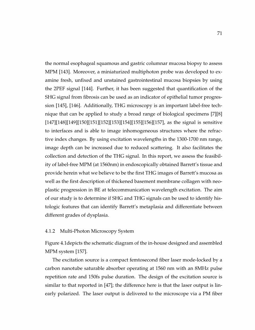
71
the normal esophageal squamous and gastric columnar mucosa biopsy to assess
MPM [143]. Moreover, a miniaturized multiphoton probe was developed to ex-
amine fresh, unfixed and unstained gastrointestinal mucosa biopsies by using
the 2PEF signal [144]. Further, it has been suggested that quantification of the
SHG signal from fibrosis can be used as an indicator of epithelial tumor progres-
sion [145], [146]. Additionally, THG microscopy is an important label-free tech-
nique that can be applied to study a broad range of biological specimens [7][8]
[147][148][149][150][151][152][153][154][155][156][157], as the signal is sensitive
to interfaces and is able to image inhomogeneous structures where the refrac-
tive index changes. By using excitation wavelengths in the 1300-1700 nm range,
image depth can be increased due to reduced scattering. It also facilitates the
collection and detection of the THG signal. In this report, we assess the feasibil-
ity of label-free MPM (at 1560nm) in endoscopically obtained Barrett’s tissue and
provide herein what we believe to be the first THG images of Barrett’s mucosa as
well as the first description of thickened basement membrane collagen with neo-
plastic progression in BE at telecommunication wavelength excitation. The aim
of our study is to determine if SHG and THG signals can be used to identify his-
tologic features that can identify Barrett’s metaplasia and differentiate between
different grades of dysplasia.
4.1.2 Multi-Photon Microscopy System
Figure 4.1depicts the schematic diagram of the in-house designed and assembled
MPM system [157].
The excitation source is a compact femtosecond fiber laser mode-locked by a
carbon nanotube saturable absorber operating at 1560 nm with an 8MHz pulse
repetition rate and 150fs pulse duration. The design of the excitation source is
similar to that reported in [47]; the difference here is that the laser output is lin-
early polarized. The laser output is delivered to the microscope via a PM fiber

72
Figure 4.1: Schematic diagram of the in-house MPM system (left) and the mul-tiphoton spectrum of Barrett Esophagus tissue (right). Red: Optical spectrum ofthe multiphoton generated signal from a normal tissue showing a strong THGsignal at 520nm. Inset: zoom-in SHG spectrum
patch cord and is collimated by using a fiber collimator (Thorlabs, F240APC-
1550); the collimated beam is then raster scanned on the sample attached to
an xyz stage by employing a 2D galvo-scanner system. A telescope consisting
of scan and tube lenses expands the beam to approximately illuminate the en-
tire back aperture of objective lens (New Focus, 5724-H-C) so that the smallest
possible laser spot size is achieved (THG resolution = 1.3µm, see [157] for res-
olution measurement). The back-scattered signal from the sample is separated
from the excitation source by a long-pass dichroic mirror with 870nm cut-off
wavelength. We use a non-descanned detection scheme enabled by a dichroic
mirror (λcut−o f f = 552nm, Semrock) and two similar high gain and sensitive
PMTs (Hamamatsu H10720-21) for simultaneously recording in two channels.
The longer wavelength channel collects the 2PEF, 3PEF or SHG signal by using
appropriate filters before the PMT. On the other hand, the shorter wavelength

73
channel collects the THG signal, where a narrow band pass filter centered at
525/30nm (Semrock) was embedded in front of the PMT. Two low-noise current
amplifiers (Stanford Research Systems, SR570) amplify the signal generated by
the PMTs before digitization by a data acquisition card (NI PCI 6110). In-house
laser scanning software based on LAbVIEW was developed was developed to
acquire images, control the image acquisition process and adjust the xyz trans-
lation stage. Each image frame was acquired and saved with 512× 512 pixels2
and a 250× 250µm2 (FOV). The frame acquisition time was 8s (pixel dwell time
of ∼ 30µs) with 15mW average power on the sample. Since the FOV was small
in comparison to the region of interest, several frames were acquired and cor-
rected for non-uniform illumination. The correction was performed by normaliz-
ing each frame by a reference frame outside the region where the sample resides.
Finally, the sequentially ordered frames were stitched by using the Stitching [158]
plugin in Fiji.
4.1.3 Methods and Sample Preparation
Cross-sectional imaging was performed on fixed tissue samples obtained by en-
doscopy from patients with Barrett’s esophagus. Tissue samples were sectioned
at 8µm, stained with hematoxylin and eosin (H&E) and evaluated independently
by two gastrointestinal pathologists. Unstained samples were obtained from a
section residing 8Âtm below the section used for histology, placed on a glass
slide with a mounting medium, and covered with a glass cover slip for MP imag-
ing. Representative samples were classified as Barrett’s esophagus (BE) with no
dysplasia (51 year old Caucasian male), BE with low-grade dysplasia (75 year old
Caucasian man) and BE with high-grade dysplasia (72 year old Caucasian male).
The institutional review board of the University of Arizona approved the study.

74
4.1.4 Results
The THG images presented herein (Figure ??) demonstrate that these label-free
images are of sufficient resolution and contrast to depict the histologic features
of BE with and without dysplasia that are seen with standard H&E stains. Of
interest, the SHG images displayed increasing thickness of the basement mem-
brane collagen with progression of the dysplasia, which is normally not seen in
H&E stains, but generally requires specific stains for displaying fibrous tissue
[159][160][161]. It should be noted that although obtained from the same biopsy
specimen and from the same patient, the multi-photon images are not as an ex-
act a match as the H&E images. Due to the 3-dimensional nature of the tissue
fragments suspended in paraffin, sequential 8µm sectioning of the tissue results
in non-identical tissue shapes and sizes, and thus a variation of appearances seen
from the same biopsy on separate slides. However, the H&E and multi-photon
images depict the same histological features from the same tissue biopsy.
4.1.4.1 Negative for Dysplasia
The THG images (Figure 4.2(e)-4.4(e)) show tissue structure with cell nuclei dis-
played with high contrast and resolution that is comparable to standard, H&E
stained microscopic images. Figure 4.2(a-d) and Figure 4.2(e-h) show the H&E
light-microscopic images and multi-photon THG images from a sample of Bar-
rett’s without dysplasia. The generation of TH signal from the surface of a mi-
croscope slide creates a bright background in THG images. Since the THG signal
is phase-matched in the forward direction, the generated forward TH signal is
larger than the backward THG signal. To detect this signal, we used a mirror un-
derneath the thin section of the tissue to redirect the forward THG signal to the
PMT. As is typical for non-dysplastic Barrett’s, the cells are positioned uniformly
in a single row along the basement membrane (Figure 4.2(f-h)). The nuclei are

75
of normal size with a normal nucleus to cytoplasm ratio. The cells with no evi-
dence of dysplasia are shown with yellow arrows in Figure 4.2. The SHG images
(Figure 4.2(i-l)) show very fine strands of sub-epithelial collagen, which cannot
be discerned in H&E images.
4.1.4.2 Low-Grade Dysplasia
Figure 4.3 shows Barrett’s with low-grade dysplasia; the cells are not all posi-
tioned in a single uniform line and the pattern of the glands remains normal.
Nuclei are stratified and mildly hyperchromatic with an increased nucleus to cy-
toplasm ratio (Figure 4.3(f-h)). These changes are shown with high contrast and
clarity in the THG images that depict all the features of the H&E findings. The
yellow arrows in Figure 4.3 represent the cells with low-grade dysplasia. The
SHG images shows thicker strands of sub-epithelial (basement-membrane) colla-
gen than in Barrett’s without dysplasia (Figure 4.2(i-l)). Note that collagen cannot
be seen in any of the color H&E images.
4.1.4.3 High-Grade Dysplasia
In Figure 4.4, the H&E and THG images exemplify high-grade dysplasia charac-
terized by marked disruption of the tissue architecture with cellular disorganiza-
tion. The nuclei are hyperchromatic and pleomorphic, with a greater increase in
the nucleus to cytoplasm ratio as well as showing loss of polarity (Figure 4.4(e-
h)). Label-free THG imaging with comparable contrast and resolution renders
the features of the H&E images. The yellow arrows in Figure 4.4 point to the cells
identified as high-grade dysplasia. In addition, the SHG images of the basement
membrane show thicker strands of sub-epithelial collagen than in Barrett’s with
low-grade dysplasia and non-dysplastic Barrett’s. Moreover, collagen is not seen
in the H&E views.

76
Figure 4.2: Comparison between multi-photon microscopy and conventionallight microscopy of BE tissue that is negative for dysplasia. (a) H&E conventionallight microscopy image showing intestinal metaplasia with goblet cells. There issurface maturation, low nucle nuclear to cytoplasmic ratio and no dysplasia. (b-d) magnified regions shown in (a). (e) High resolution THG signal from MPMand (f-h) the magnified regions in (e). (i) SHG signal recorded simultaneouslywith the THG signal showing collagen distribution in the stroma and blood ves-sels. (j-l) magnified marked regions in the SHG image to show collagen in thebasement membrane. The THG signal has a clear correlation to the H&E light-microscope image. The architectural structure of nuclei indicates that the tissuehas no dysplastic feature. The yellow arrows show the cells with no evidence ofdysplasia. (FOV in (e) and (i): 1000× 750µm2, acquisition time: 2min)

77
Figure 4.3: Multi-photon and conventional light microscopy images for low-grade dysplastic BE tissue. (a) Conventional light microscopy image of the tissuestained with H&E; there is intestinal metaplasia with goblet cells, surface luminalcells displaying nuclear stratification, hyperchromasia, and an increased nuclearto cytoplasmic ratio (N: C). (b-d) magnified regions marked in the H&E image. (e-h) High resolution THG images that show features of low-grade dysplasia in thesame biopsy. (i-l) corresponding simultaneous SHG signals of the THG imagesthat display the presence of collagen. The spatial distribution of cell nuclei is con-sistent with low-grade dysplasia. The cells with low-grade dysplasia are markedwith arrows. (FOV in (e) and (i): 750× 1000µm2, acquisition time: 2min). Thevertical white lines in (j)-(l) are the PMT artifacts

78
Figure 4.4: MPM and conventional light microscopy images of high-grade dys-plastic tissue. (a) Conventional light microscopy image of the tissue after labelingwith H&E. There is a progressive dysplastic change in a background of intesti-nal metaplasia. Cells have marked hyperchromatic nuclei nuclear stratification,loss of polarity and a markedly increased N:C ratio, considerably more than inlow grade dysplasia. (b-d) magnified squared regions marked in (a). (e) Highresolution THG and (f-h) corresponding magnified regions. (i) High resolutionSHG image and (j-l) the magnified regions marked in to show basement mem-brane collagen (i). The dense nuclei with variable shapes and sizes as well as theloss of orderly arrangement of the cells are consistent with high-grade dyspla-sia. Arrows represent the cells with high-grade dysplasia. (FOV in (e) and (i):500× 500µm2, acquisition time: <1min)

79
4.1.4.4 Basement membrane collagen
The SHG images acquired simultaneously with the THG images in this study
show thickening of sub-epithelial (basement membrane) collagen with advancing
stages of dysplasia. Figure 4.5 shows the same SHG images of different stages of
the dysplasia shown in Figure 4.2-4.4 when contrast adjusted by using Fiji. In
each image (Figure 4.5(a-c)), three areas of sub-epithelial collagen were chosen
(A, B, C) and the thickness measured increased progressively with advancing
grades of dysplasia, with marked thickening in high-grade dysplasia.
4.1.5 Discussion
This initial work indicates the potential of MPM in generating label-free images
of Barrett’s mucosa with contrast and clarity that is equal, if not superior, to tra-
ditional H&E microscopy enabling a histologic diagnosis to be made. Further-
more, the imaging of the sub-epithelial basement membrane evidences increas-
ing thickness of collagen with progression of dysplasia, most prominently in the
high-grade form. The increased thickness of basement membrane collagen may
represent the body’s response to carcinogenesis by attempting to prevent inva-
sion of cells into deeper layers as the disease progresses to cancer. Noting that this
observation has been made in a small sample and the findings need to be verified
in a larger study, we believe that the implied capability of the SHG MPI to selec-
tively image basement membrane collagen may enable it to become a quantifiable
tool for the identification of high-grade dysplasia, which would be of great clin-
ical value. Histological sample preparation and examination by a pathologist to
identify the morphological features of a suspicious biopsy in conventional H&E
light microscopy are not only time-consuming and burdensome; a diagnosis can-
not be made in-vivo or at the point of care. MPM has the advantage of being able
to provide high quality images ex-vivo or in-vivo and at the point of care. Fur-

80
Figure 4.5: SHG signal from Barrett’s with non-dysplastic dysplasia (a), lowgrade dysplasia (b) and high grade dysplasia (c). Corresponding graphs to theright show the thickness of the basement membrane collagen measured at eachof the three chosen points per image, which confirm increasing thickness withprogression of dysplasia

81
thermore, MPM should be able to image sub-epithelial buried glands and detect
early invasion of cancer in reconstructed 3D images as well as 2D views.
4.1.6 Conclusion
We believe these to be the first reported THG images of Barrett’s esophagus for
demonstration of MPI to identify diagnostic features of low- and high-grade dys-
plasia in Barrett’s. We also report on thickened basement membrane collagen in
dysplastic Barrett’s epithelium in SHG images, which may prove to be a comple-
mentary diagnostic marker of disease stage. Our preliminary results suggest that
label-free THG and SHG images may provide not only a substitution for H&E
histology in Barrett’s, but the future construction of a fiber-optic probe may en-
able in-vivo detection of unseen dysplasia or cancer during endoscopy and guide
therapy, such as endoscopic mucosal resection and radio-frequency ablation.
4.2 Multiphoton microscopy as a detection tool for photobleaching of EO
4.2.1 Introduction
The photochemical properties of materials are of crucial importance for their ac-
ceptance in commercial optical systems. Nowadays, pulsed lasers with high peak
intensities are widely used in different optical devices, where the high laser in-
tensities can cause materials to undergo photochemical reactions and remove
molecules from the population. This process is called photobleaching and is
caused by transitions between excited states of different multiplicity as well as
chemical reactions, interaction with the environment and interaction with the
excitation light [162][163]. In general, the photostability of a material dictates
its suitability for a particular application and molecules with diverse photo-
chemical properties are required for different optical systems. Highly photo-
stable molecules are needed for applications such as optical modulators and

82
switches while materials with a large photobleaching rate are needed for three-
dimensional read-write devices [164][165]. Thus, for successful device fabrication
it is crucial to characterize the materials’ photostability properties to ensure the
best device performance and yield. Standard optical characterization techniques
such as optical microscopy and Raman spectroscopy [166] are time-consuming
and not suitable for rapid characterization in large scale samples. Furthermore,
these techniques only indicate a change in materials shape and molecular struc-
ture and do not elucidate the bleaching mechanisms. From the discussion above,
the need for a better method of understanding the probability and mechanisms of
photobleaching of various materials at a specific applied excitation irradiance is
clear. Multi-photon microscopy (MPM) is a powerful technique that allows map-
ping of thin film samples with any kind of optical response such as multi-photon
fluorescence (MPFL), second-, and third-harmonic generation (SHG, THG). There
are several reports that discuss the measurement of the photobleaching of mate-
rials by observing the decrease of the fluorescence intensity using two-photon
imaging [110][167][168]. However, these studies are limited only to fluorescent
materials. The number of photons involved in the bleaching process can be deter-
mined by investigating the bleaching rate versus the excitation irradiance. Many
researchers have worked to gain a better understanding of photobleaching in the
case of one- and two-photon excitations [169][170]. However, only a few reports
are available on photobleaching in the case of three- and more photon excitation
[164]. Further, most previous works have been carried out at the wavelengths in
the visible range of spectrum which makes it difficult to detect two-, and three-
photon ex- citation signals due to the lack of optical components such as lenses
and objectives with high sensitivity in the UV regime.
We have in this article successfully employed a multi-photon microscope with
a compact femtosecond fiber laser at 1550nm to explore electro-optical (EO) ma-
terials suitability in terms of photostability for optical devices such as waveg-
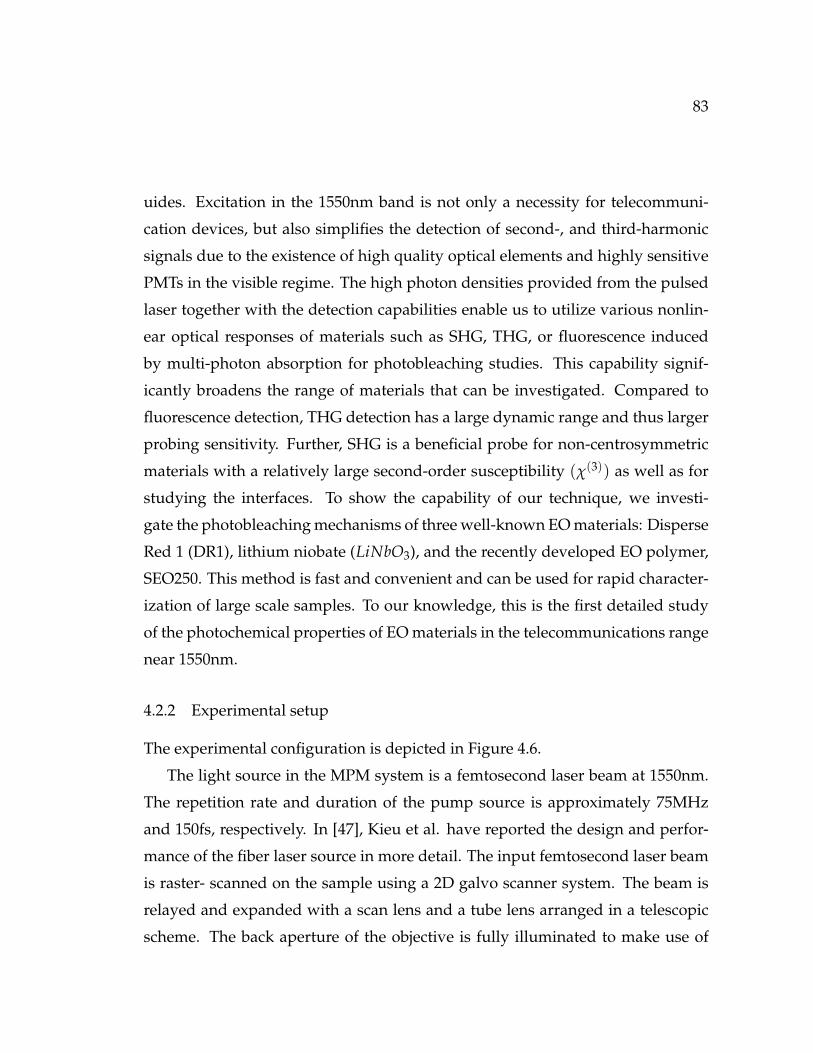
83
uides. Excitation in the 1550nm band is not only a necessity for telecommuni-
cation devices, but also simplifies the detection of second-, and third-harmonic
signals due to the existence of high quality optical elements and highly sensitive
PMTs in the visible regime. The high photon densities provided from the pulsed
laser together with the detection capabilities enable us to utilize various nonlin-
ear optical responses of materials such as SHG, THG, or fluorescence induced
by multi-photon absorption for photobleaching studies. This capability signif-
icantly broadens the range of materials that can be investigated. Compared to
fluorescence detection, THG detection has a large dynamic range and thus larger
probing sensitivity. Further, SHG is a beneficial probe for non-centrosymmetric
materials with a relatively large second-order susceptibility (χ(3)) as well as for
studying the interfaces. To show the capability of our technique, we investi-
gate the photobleaching mechanisms of three well-known EO materials: Disperse
Red 1 (DR1), lithium niobate (LiNbO3), and the recently developed EO polymer,
SEO250. This method is fast and convenient and can be used for rapid character-
ization of large scale samples. To our knowledge, this is the first detailed study
of the photochemical properties of EO materials in the telecommunications range
near 1550nm.
4.2.2 Experimental setup
The experimental configuration is depicted in Figure 4.6.
The light source in the MPM system is a femtosecond laser beam at 1550nm.
The repetition rate and duration of the pump source is approximately 75MHz
and 150fs, respectively. In [47], Kieu et al. have reported the design and perfor-
mance of the fiber laser source in more detail. The input femtosecond laser beam
is raster- scanned on the sample using a 2D galvo scanner system. The beam is
relayed and expanded with a scan lens and a tube lens arranged in a telescopic
scheme. The back aperture of the objective is fully illuminated to make use of

84
Figure 4.6: The schematic of the multi-photon microscope, and b) diagram show-ing various sources and probes on materials photodegradation study
the full NA (NA=0.5, 20× aspheric objective lens) and create the smallest possi-
ble laser spot size on the sample (confocal parameter=7.2µm, spot size=1.4µm).
The backscattered signals are detected simultaneously using two highly sensitive
high gain PMTs through a series of dichroic beam splitters and filters. A nar-
row bandpass filter ( 20nm FWHM bandwidth) is used before each of the PMTs
to detect the SHG ( 780 nm) and THG ( 520 nm) generated from the laser focal
spot. The fluorescence due to two- or three-photon excitation can be measured
by removing the 780nm bandpass filter from the transmission path of dichroic
mirror. The generated multi-photon signals can also be detected with a sensitive
spectrometer with the use of a rotating dichroic mirror at 870nm. The diagram
shown in Figure 4.6(b) demonstrates the main mechanisms (single-, two-, and
three- photon excitation, photo-oxidation and temperature increase) involved in
material degradation when pulsed lasers with high peak intensities are used. It
further shows the various probes that can be utilized by our MPM system to
study material photobleaching, among which the FL emission is the most stud-
ied probe so far. As explained above, with the various probes available, we have
the capability to study the photostability of a broad range of materials needed for
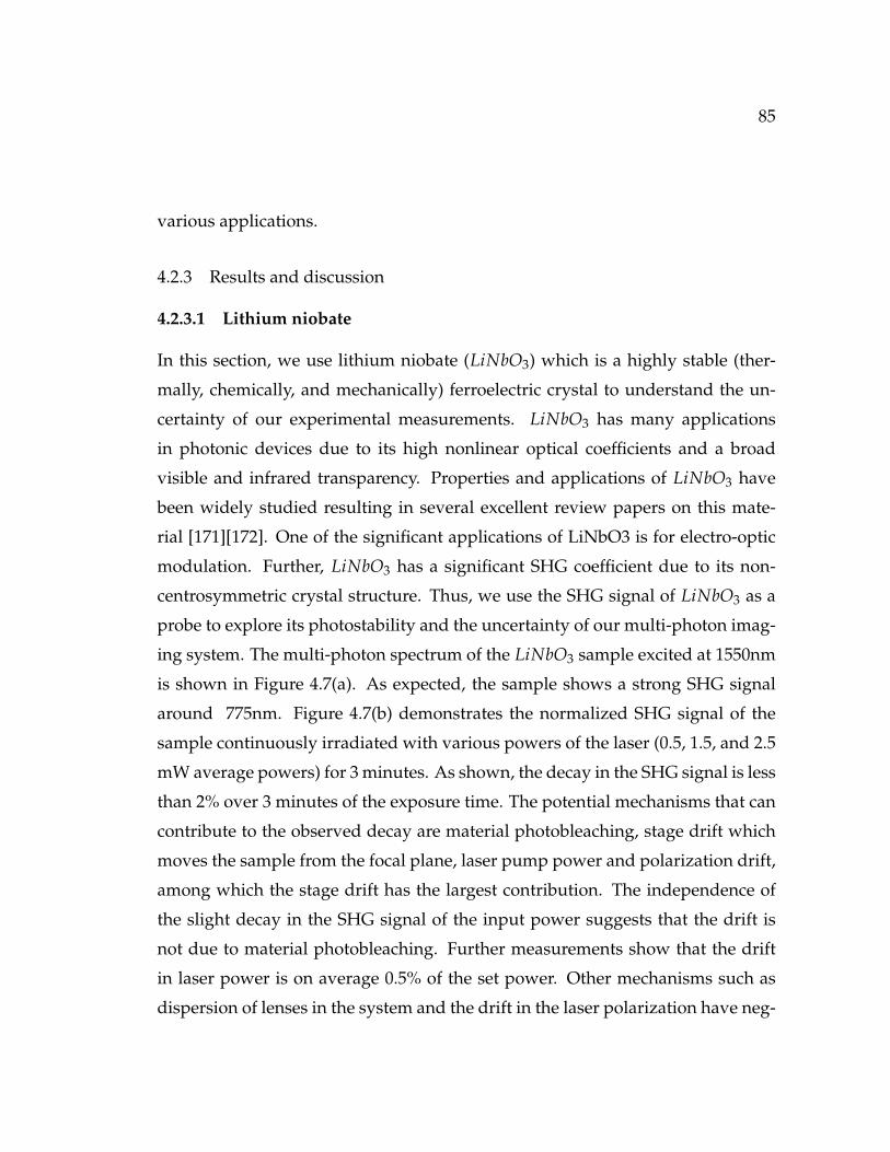
85
various applications.
4.2.3 Results and discussion
4.2.3.1 Lithium niobate
In this section, we use lithium niobate (LiNbO3) which is a highly stable (ther-
mally, chemically, and mechanically) ferroelectric crystal to understand the un-
certainty of our experimental measurements. LiNbO3 has many applications
in photonic devices due to its high nonlinear optical coefficients and a broad
visible and infrared transparency. Properties and applications of LiNbO3 have
been widely studied resulting in several excellent review papers on this mate-
rial [171][172]. One of the significant applications of LiNbO3 is for electro-optic
modulation. Further, LiNbO3 has a significant SHG coefficient due to its non-
centrosymmetric crystal structure. Thus, we use the SHG signal of LiNbO3 as a
probe to explore its photostability and the uncertainty of our multi-photon imag-
ing system. The multi-photon spectrum of the LiNbO3 sample excited at 1550nm
is shown in Figure 4.7(a). As expected, the sample shows a strong SHG signal
around 775nm. Figure 4.7(b) demonstrates the normalized SHG signal of the
sample continuously irradiated with various powers of the laser (0.5, 1.5, and 2.5
mW average powers) for 3 minutes. As shown, the decay in the SHG signal is less
than 2% over 3 minutes of the exposure time. The potential mechanisms that can
contribute to the observed decay are material photobleaching, stage drift which
moves the sample from the focal plane, laser pump power and polarization drift,
among which the stage drift has the largest contribution. The independence of
the slight decay in the SHG signal of the input power suggests that the drift is
not due to material photobleaching. Further measurements show that the drift
in laser power is on average 0.5% of the set power. Other mechanisms such as
dispersion of lenses in the system and the drift in the laser polarization have neg-
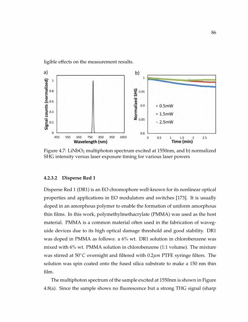
86
ligible effects on the measurement results.
Figure 4.7: LiNbO3 multiphoton spectrum excited at 1550nm, and b) normalizedSHG intensity versus laser exposure timing for various laser powers
4.2.3.2 Disperse Red 1
Disperse Red 1 (DR1) is an EO chromophore well-known for its nonlinear optical
properties and applications in EO modulators and switches [173]. It is usually
doped in an amorphous polymer to enable the formation of uniform amorphous
thin films. In this work, polymethylmethacrylate (PMMA) was used as the host
material. PMMA is a common material often used in the fabrication of waveg-
uide devices due to its high optical damage threshold and good stability. DR1
was doped in PMMA as follows: a 6% wt. DR1 solution in chlorobenzene was
mixed with 6% wt. PMMA solution in chlorobenzene (1:1 volume). The mixture
was stirred at 50◦C overnight and filtered with 0.2µm PTFE syringe filters. The
solution was spin coated onto the fused silica substrate to make a 150 nm thin
film.
The multiphoton spectrum of the sample excited at 1550nm is shown in Figure
4.8(a). Since the sample shows no fluorescence but a strong THG signal (sharp

87
Figure 4.8: Multiphoton spectrum of DR1 on fused silica, the inset shows thelog-log plot of the output THG signal versus input power, b) normalized THGintensity versus exposure timing for various laser powers, and c) THG profile ofthe sample where each square
peak at 517nm), we use THG as a probe to explore the photobleaching mech-
anism of DR1 (the cubic dependence of the output power on the input pump
shown in the inset also indicates that the probe is THG signal). Figure 4.8(b)
demonstrates the normalized THG signal reflected back from the sample when
it is continuously irradiated with the focused laser beam at 1550 nm for 3 min-
utes. The THG profile of the sample is shown in Figure 4.8(c) where several areas
of the sample (26µm × 26µm squares, 512 × 512 pixels2) each continuously ex-
posed by various powers and timings of the laser are shown. It can be seen that
at very low irradiation power (below 8mW), photobleaching is negligible. How-
ever, for excitation peak power values greater than 8mW, the process of photo-
bleaching becomes significant and a decay of the THG is observed. In order to fit
our experimental data for THG signal, we tried three different functions: single-,
double-, and stretched-exponential. The results of Figure 4.9(a) demonstrate that
both double- and stretched- exponential functions could fit the data with good
agreement. It should be noted that several relaxation phenomena in complex
condensed-matter systems have been found to follow the stretched-exponential
decay law. Specially, dielectric relaxation in polymers are usually described as

88
being a stretched-exponential function [174]. Although a large weight percent-
age of polymer is used in DR1 samples, we chose to fit the experimental results
with a double exponential since that would make the interpretation of the two
well-known degradation phenomena in DR1 (photo-oxidation and tran-cis iso-
merization) easier. A double-exponential decay function can be written as [111]:
T = T0 + T1e−k1t + T2e−k2t (4.1)
Figure 4.9: DR1 decay curve with 30mW power (circle-marked line), best fittedone- (dash- dotted line), double-(dotted line), and stretched-exponential (solidline) functions, b) log- log plots of the photobleaching rates k1 and k2 vs. irradia-tion power, and c) the ratio between parameters k1 and k2 (left axis) and A1 andA2 (right axis) vs irradiation power
In this expression T is the THG photon flux, k1 and k2 are the rates of de-
crease of THG signal, called here photobleaching rates (1/s), T1 and T2 are the
initial contributions to the THG signal from each exponential decay (photon/s),
and T0 is a noise constant. The two exponential decay rates in the bleaching
function represents two different mechanisms involved in the photobleaching
process of DR1. The photobleaching rates k1 and k2 versus irradiation power
are depicted in Figure 4.9(b). As can be seen, the slopes of logarithmic plots are
0.61 and 1.26 for k1 and k2, respectively. Hence, the slopes of the photobleaching
rates suggest that a one-photon process is the bleaching source for both mech-

89
anisms. It is shown in Figure 4.9(c) that the first mechanism associated with k1
is a much faster process compared to the second mechanism (k1 � k2). On the
other hand, the contribution to the THG signal from the two mechanisms is com-
parable. As mentioned earlier, the dominant degradation mechanisms in DR1
are photo-oxidation and tran-cis isomerization [175][176]. The photo-oxidation
(described by the first mechanism with decay rate of k1 is due to triplet ground
state oxygen molecules that absorb infrared photons and become singlet oxygen
free-radical species that aggressively attack the chromophores. Further, tran-cis
isomerization which leads to statistical photo-orientation of the DR1 molecules,
is a relatively slow process described by the second mechanism with decay rate
of k2.
4.2.3.3 SEO250
SEO250 is a popular EO polymer, which also has a relatively large χ(3) and negli-
gible fluorescence when it is unpoled (the emission spectrum is shown in Figure
4.10(a) with a strong signal at 517nm and no fluorescence).
A prime application of this polymer is in EO channel waveguide devices.
SEO250 is highly photostable with negligible photobleaching in the ultravio-
let regime of the spectrum and the ability to transmit on the order of 50mW
of CW 1550nm for hundreds of hours well beyond what is needed for most
optical communication applications. The sample was fabricated by dissolving
SEO250 3% wt. in dibromomethane and leaving it to stir overnight, then a
350 nm thick film was fabricated by spin coating the solution on a fused sil-
ica substrate. Figure 4.10(b) shows the normalized photobleached THG sig-
nal reflected back from the sample versus exposure time for different excita-
tion powers. The THG profile of the sample is demonstrated in Figure 4.10(c)
with 16 squares (26µm× 26µm, 512× 512 pixels2) each continuously exposed by
laser powers ranging from 9-25 mW and 15, 30, 60, and 120 sec exposure times

90
Figure 4.10: Multiphoton spectrum of SEO250 on fused silica, the inset shows aUV/Vis absorption spectrum of SEO250 (top) and the log-log plot of the outputTHG signal versus input power (bottom), b) normalized THG intensity versuslaser exposure timing for various laser powers, and c) THG profile of the sam-ple where each square is continuously exposed by a different laser power andexposure timing
(∼ 0.5 f rame/sec). As can be seen in this figure, the observed bleaching has a
clear correlation to the amount of laser power as well as to the total duration of
the exposure. Figure 4.11(a) demonstrates that the THG decay of SEO250 versus
time could be fitted by both a double-exponential and a stretched-exponential.
However, consideration of the relative decay rate and amplitude of the two in-
troduced mechanisms when a double-exponential decay law is used, indicates
that there is likely a single process for the photobleaching. Figure 4.11(b) demon-
strates a log-log plot of the photobleaching rates (k1 and k2) versus laser power
and the ratio of the two mechanisms contribution (shown in the inset) when a
double-exponential is used. The slopes of the logarithmic plots (2.27 for k1 and
1.95 for k2) show that bleaching for both mechanisms is due to a two-photon exci-
tation source since both photobleaching rates depend on square of the excitation
power. Further, it can be seen that the two mechanisms are comparable in their
speed and contribution. Thus, we chose to use a stretched-exponential function
to describe the bleaching mechanism of SEO250:

91
T = T0e−ktβ(4.2)
Figure 4.11: a) Fitting SEO250 decay curve with 19.8 mW power (circle-markedline) with 1- (dash-dotted line), 2-(dotted line), and stretched-(solid line) expo-nential functions. b) log- log plots of the photobleaching rates k1 and k2 forSEO250, inset: the ratio between parameters A1 and A2 vs irradiation power,and c) the photobleaching rate versus irradiation power when the experimentaldata was fitted with a stretched-exponential function
where T is the THG photon flux, k is the photobleaching rate (1/s), and
0 < β < 1 is a dispersive factor. The slope 2.11 of the plot shown in Fig-
ure 4.11(c) demonstrates that as expected from the double-exponential model,
only two photons are involved in the bleaching process and that the degrada-
tion mechanism is two-photon excitation. This is consistent with the fact that the
SEO250 EO chromophore has intense one-photon absorption at 775nm and the
non- centrosymmetric nature of the chromophore relaxes the usual parity driven
one and two-photon absorption selection rules.
4.2.4 Conclusion
In summary, the photobleaching of three electro-optical materials (lithium nio-
bate, Disperse Red 1, and SEO250) was explored under ultrashort pulsed illumi-
nation at 1550nm using multi- photon microscopy. One-photon and two-photon
92
excitation have been identified as the main bleaching mechanisms for DR1 and
SEO250, respectively. Further, the large chemical stability of LiNbO3 has been
confirmed. This method is designed to be a rapid screening test to assist in the de-
velopment of new materials and to properly target them for applications. More-
over, it can be realized on a broad range of materials using detection probes such
as multi-photon excitation FL, SHG, and THG. Furthermore, the involvement of
two, three, or even more photons in the bleaching process can be explored. The
main application of this work is in the design of various optical devices such as
channel waveguides, EO modulators, etc., where by choosing suitable conditions
for device performance, such as excitation threshold and the type of material,
fabrication with optimum performance and yield is feasible.
4.3 Multi-photon microscopy for characterization of 2D materials
Besides biological and photobleaching monitoring applications, we used our
MPM to characterize electro-optic (EO) polymers used in Si-photonic devices
[176] . In this project, we imaged phase modulators consisting of silicon waveg-
uide devices with EO polymer cladding and measured the SHG intensity using
MPM and correlated this intensity with Pockels coefficient (r33) measurement.
This allowed us to map out r33 locally and make quantitative measurements of
poled polymer films on non-transparent silicon substrates which is not accessi-
ble with conventional Pockels coefficient measurement techniques. Figure 4.12
below shows the MPM images and the quantitative comparison between SHG
intensity and r33 values.
Using MPM enables rapid characterization and measurement of the Pockels
coefficient and may open up a new window to utilize MPM for such application
in photonics. Moreover, it can be used for rapid poling optimization by changing
laser power, scanning speed and incident light polarization.

93
Figure 4.12: (a) Composite of SHG (red) and THG (green), (b) SHG in the poledregion, (c) THG from on top of the gold electrodes. The orange box in (b) indicatesthe region in which the quantitative SHG data was collected. (d) Ratio of themeasured r33 to the square root
Figure 4.13: Typical multiphoton micrographs of a sample containing exfoliatedgraphene on SiO2/Si substrate. (a) Fluorescence, (b) third-harmonic signal, and(c) merged RGB image using fluorescence (red) and THG (green) signals. Oneparticularly interesting few-layer graphene flake considered below is markedwith white circles and shown magnified in the merged RGB image

94
MPM can also be used to characterize 2D materials [100][101][102]. 3PEF and
THG signals were used to map out and characterize 2D materials like graphene,
GaSe and GaTe. The contrast between the 2D material and substrate appears
in THG signal where there is refractive index mismatch or interface between
the structures. We showed that MPM can be used as a rapid and noninvasive
technique to distinguish between single- and bi-layer graphene in a few seconds
compared to the time-consuming and slow conventional technique like Raman
microscopy [100]. Besides the speed of scanning, one can map out a larger FOV
(500µm× 500µm) compared to 50µm× 50µm one in Raman. Figure 4.13 shows
the typical multi-photon images of a sample containing exfoliated graphene on
SiO2/Si substrate. As can be seen, 3PEF and THG signal provide different in-
formation about the sample based on the nature of excitation wavelength and
emitted signal. In the flakes shown inside the marked circle the contrast between
single- and bi-layer areas are readily observable. Figure 4.14 also indicates the
power of THG signal on distinguishing different layers of graphene. In this graph
the THG intensity was plotted versus the laser power on the sample for different
number of layers available on the exfoliated sample. According to the data points
and exponential fitted curves, there is almost cubic dependency of the THG sig-
nal to the incident power.
We also used SHG and THG signals to investigate the nonlinear optical prop-
erties of GaSe which is a 2D layered semiconductor material with a well-known
optical crystal [101]. We compared MPM images with standard characterization
tools like AFM and Raman measurements to validate our finding. Figure 4.15
presents the SHG and THG signals from a few-layer GaSe flake. The multipho-
ton emission spectra of different layers were also shown in Figure 4.15(e). Note
that SHG and THG provide slightly different information about the layers as can
be seen in (c) and quantitative measurement in (d).
Figure 4.16 shows the power dependency curves for SHG and THG signals

95
Figure 4.14: Dependence of the THG peak signal on the laser peak power andnumber of graphene layers. Dots are measurement values; the curves are expo-nential fits to the power dependence. In the logarithmic plot in the inset, threepoints corresponding to the lowest THG power deviate from the general trendbecause the power level is below the linear regime of our detection system

96
Figure 4.15: (a) SHG and (b) THG images of the few-layer GaSe flake, (c) RGBcomposite image generated from the SHG and THG images, and (d) cross-sections of the SHG and THG signals taken from the white dashed line in (c).The spectra of the generated light have been measured from the points markedwith Roman numbers II, V and VII in (c). (e). Measured spectra of the gener-ated light from three different positions (different thicknesses) on the flake. Thepositions are marked by Roman numbers II, V and VII

97
versus the incident power. The slopes of 2 and 3 in the log-log plots ensures the
harmonic process. Figure 4.16(c) is the SHG and THG peak powers versus the
number of detected layers. According to this graph, the SHG and THG intensity
increase with the number of layers. However, it should be noted that based on
theory the reflected SHG and THG signals have sinc-like behavior for reflection
mode. Through the reflected SHG and THG coherence length, the maximum
SHG and THG signal can be calculated and the corresponding number of layers
can be extracted. The reflected SHG and THG coherence length can be calculated
as:
lBSHGc =
λ
4(n(2ω) + n(ω))=
1560nm4(2.75 + 2.85)
= 70nm (4.3)
lBTHGc =
λ
6(n(3ω) + n(ω))=
1560nm6(2.75 + 3.19)
= 45nm (4.4)
In which n is the refractive index at the subscript frequency. Therefore, for
layers with thicknesses of below the coherence length the SHG and THG signals
increase monotonically. For layers larger than these values the intensities de-
crease. Note that this sinc-like behavior is periodic and for larger thicknesses, the
SHG and THG intensities increase and then decrease.
Figure 4.16: Power dependence of the (a) SHG and (b) THG signals. (c) SHG andTHG signals as a function of the number of the GaSe layers measured with 1kWexcitation peak power
Similarly, we performed the same study for another 2D semiconductor mate-

98
rial, GaTe [103]. SHG and THG images as well as AFM micrograph are shown
in Figure 4.17. The calculated coherence lengths for SHG and THG signals are
34nm and 46nm, respectively. According to SHG and THG intensities versus the
excitation peak power show that for the layer thicknesses below the coherence
lengths, the peak powers increase monotonically, while for layers thicker than
the coherence lenght there is a decreasing trend. The nonlinear susceptibilities of
2D materials can be calculated using SHG and THG signals showing the power-
ful capability of MPM for rapid and accurate material characterization.
Figure 4.17: (a) SHG and (b) THG images of the few-layer GaTe flake. (c) RGBcomposite image generated from the SHG and THG images. (d) Cross-sectionalSHG and THG signals taken from the blue dashed line in (c); scale bars in theSHG and THG images are 10µm. (e) AFM image of the staircase area where theintensity is at maximum for both SHG and THG. (f) AFM cross-section of thestaircase area taken from the white dashed line B-B’ in (e) showing the steps from17 to 57nm. Excitation peak power dependence of the (h) SHG and (i) THG sig-nals. The lines are fits to square (h) and cubic (i) power dependences
In another experiment, THG signal was used to characterize the third-order
nonlinearity of high-quality nanocrystalline titanium dioxide (TiO2) made with
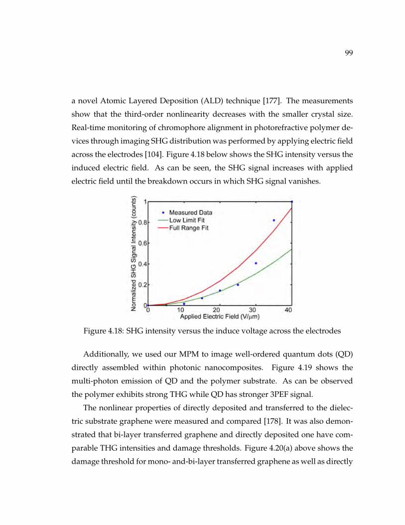
99
a novel Atomic Layered Deposition (ALD) technique [177]. The measurements
show that the third-order nonlinearity decreases with the smaller crystal size.
Real-time monitoring of chromophore alignment in photorefractive polymer de-
vices through imaging SHG distribution was performed by applying electric field
across the electrodes [104]. Figure 4.18 below shows the SHG intensity versus the
induced electric field. As can be seen, the SHG signal increases with applied
electric field until the breakdown occurs in which SHG signal vanishes.
Figure 4.18: SHG intensity versus the induce voltage across the electrodes
Additionally, we used our MPM to image well-ordered quantum dots (QD)
directly assembled within photonic nanocomposites. Figure 4.19 shows the
multi-photon emission of QD and the polymer substrate. As can be observed
the polymer exhibits strong THG while QD has stronger 3PEF signal.
The nonlinear properties of directly deposited and transferred to the dielec-
tric substrate graphene were measured and compared [178]. It was also demon-
strated that bi-layer transferred graphene and directly deposited one have com-
parable THG intensities and damage thresholds. Figure 4.20(a) above shows the
damage threshold for mono- and-bi-layer transferred graphene as well as directly

100
Figure 4.19: Normalized multiphoton excitation spectra and micrographs of (a)the blend of BBCP D with 30 wt % QDs and (b) neat polymer sample. The wave-length of light for excitation was 1550nm
deposited graphene. Figure 4.20(b, c) also depicts THG images of these two sam-
ples.
In an experiment, silicon surface was patterned on nanoridge array waveg-
uides and the sample was illuminated by 1550nm excitation wavelength [179].
The THG signal for different trench and ridge geometries were measured and
plotted in Figure 4.21(b). It was shown that for larger ridge sizes the THG in-
creases. Moreover, the effect of incident light polarization on the THG signal was
investigated. Figure 4.21(c) shows the THG signal for TE and TM polarizations.
As expected for TE polarization THG is maximum while for TM polarization it
reaches its minimum.
Finally, two-photon microscopy was used to compare the enhancement of
2PEF from three chromophores by fabricating grating substrate having the res-
onance frequency tuned to the 1040nm excitation wavelength [180]. Figure 4.22
below shows the 2PEF images of rhodamine 6G, GFP and chlorophyll across the

101
Figure 4.20: Damage threshold of directly deposited graphene is comparable tomono- and bi-layered graphene prepared by the transfer technique. ÎTIntensity isthe intensity difference of THG signal between the studied area and the referencearea. The damage area has less THG than the pristine area. Multiphoton micro-scopic images of (a) transferred graphene film with a tear and folded areas and (b)directly deposited graphene with a scratch made by a scalpel. (a-inset) averagegraphene film thickness is comparable to folded bi-layered graphene prepared bytransfer technique. (Both image size is about 300× 300µm2. Color bar indicatesthe intensity of THG signal.)
boundaries between the textured and planar substrates.
The comparison between 2PEF from planar and textured areas are also shown
in Figure 4.23.

102
Figure 4.21: (a) Optical setup used to measure the third-harmonic signal of thesilicon samples. (b) Measured third-harmonic spectra for the samples with dif-ferent trench and ridge geometries. (c) THG signal as a function of the angle ofpolarization of the input be beam. (d) Spatially resolved optical images of thethird-harmonic signal for two orthogonal polarizations of the input beam

103
Figure 4.22: Multiphoton microscope images of the boundaries between textured(left) and planar (right) substrates coated with rhodamine 6G (a), green fluores-cent protein (b), and chlorophyll (c)
Figure 4.23: Fluorescence signals (left column) and enhancements (right column)calculated from the MPM measurements. The inset shows five images of the R6Gsample at different focus positions

104
CHAPTER 5
Summary
In this dissertation I described the theory of multiphoton microscopy and multi-
photon imaging modalities including SHG, THG, 2PEF and 3PEF. The full design
and assembly of a compact MPM was explained in details starting from the op-
tical design of a relay lens system, compound scan tube lenses. A laser scanning
LabVIEW-based software was also developed to acquire, save and manipulate
the images. Throughout the application section, a novel methodology based on
nonlinear response of a sharp edge of GaAs wafer was introduced to character-
ize the objective lenses used in MPM. This method is originated from a known
technique called "knife edge"; however, here we expanded this technique to the
nonlinear regime. Different imaging modalities were utilized to investigate the
biological samples in response to femtosecond illumination. A clear correlation
between label-free THG images and conventional H&E light microscopy images
were found in [99]. Moreover, it was shown that SHG is an alternative modal-
ity that can be used to help pathologists distinguish between different stages of
cancer progress. THG signal was also used to monitor the photobleaching of
EO polymers under femntosecond illumination at certain powers and pulse du-
rations [4]. The decay in THG signal can indicate the life-time of EO polymer
which can be used for manufacturing of the modulators used in telecommuni-
cation systems. MPM can also be used to characterize the optical properties of
2D materials such as Graphene [100], GaSe [101] and GaTe [102]. This brought
a rapid and accurate methodology for 2D materials characterization in the field
which can be replaced for slow characterization techniques such as Raman, SEM
or AFM. The wide range of MPM applications make MPM a promising tool for

105
studies of not only biological samples but also optical characterization of 2D ma-
terials. Currently, new applications of MPM are discovered every day showing
that MPM is on its path to be used widespread; however, a few limitations in laser
source size and cost, optimum optical design and detection have to be addressed
before it becomes widely used in special applications such as clinical diagnosis.

106
REFERENCES
[1] Warren R Zipfel, Rebecca M Williams, and Watt W Webb. Nonlinear
magic: multiphoton microscopy in the biosciences. Nature biotechnology,
21(11):1369–1377, 2003.
[2] Soroush Mehravar, Bhaskar Banerjee, Hemant Chatrath, Babak Amirso-
laimani, Krunal Patel, Charmi Patel, Robert a Norwood, Nasser Peygham-
barian, and Khanh Kieu. Label-free multi-photon imaging of dysplasia in
Barrett’s esophagus. Biomedical Optics Express, 7(1):148, 2016.
[3] Kaitlin Harpel, Robert Dawson Baker, Babak Amirsolaimani, Soroush
Mehravar, Josef Vagner, Terry O. Matsunaga, Bhaskar Banerjee, and Khanh
Kieu. Imaging of targeted lipid microbubbles to detect cancer cells using
third harmonic generation microscopy. Biomedical Optics Express, 7(7):2849,
2016.
[4] Shiva Shahin, Soroush Mehravar, Palash Gangopadhyay, Nasser Peygham-
barian, Robert. a. Norwood, and Khanh Kieu. Multiphoton microscopy
as a detection tool for photobleaching of EO materials. Optics Express,
22(25):30955–30962, 2014.
[5] M. J. Levene. In Vivo Multiphoton Microscopy of Deep Brain Tissue. Journal
of Neurophysiology, 91(4):1908–1912, 2004.
[6] Fritjof Helmchen, Karel Svoboda, Wilfred Denk, and David W. Tank. In
vivo dendritic calcium dynamics in deep-layer neocortical pyramidal neu-
rons. Nature, 2:989–996, 1999.

107
[7] Nicholas G. Horton, Ke Wang, Chun Chin Wang, and Chris Xu. In vivo
three-photon imaging of subcortical structures of an intact mouse brain
using quantum dots. 2013 Conference on Lasers and Electro-Optics Europe
and International Quantum Electronics Conference, CLEO/Europe-IQEC 2013,
7(March):205–209, 2013.
[8] Matthew J. Farrar, Frank W. Wise, Joseph R. Fetcho, and Chris B. Schaf-
fer. In vivo imaging of myelin in the vertebrate central nervous system us-
ing third harmonic generation microscopy. Biophysical Journal, 100(5):1362–
1371, 2011.
[9] Evan P. Perillo, Justin E. McCracken, Daniel C. Fernée, John R. Goldak,
Flor a. Medina, David R. Miller, Hsin-Chih Yeh, and Andrew K. Dunn.
Deep in vivo two-photon microscopy with a low cost custom built mode-
locked 1060 nm fiber laser. Biomedical Optics Express, 7(2):324, 2016.
[10] Ryosuke Kawakami, Kazuaki Sawada, Aya Sato, Terumasa Hibi, Yuichi
Kozawa, Shunichi Sato, Hiroyuki Yokoyama, and Tomomi Nemoto. Visu-
alizing hippocampal neurons with in vivo two-photon microscopy using a
1030 nm picosecond pulse laser. Scientific reports, 3:1014, 2013.
[11] Timothy Ragan, Lolahon R Kadiri, Kannan Umadevi Venkataraju, Karsten
Bahlmann, Jason Sutin, Julian Taranda, Ignacio Arganda-Carreras, Yongsoo
Kim, H Sebastian Seung, and Pavel Osten. Serial two-photon tomography
for automated ex vivo mouse brain imaging. Nature Methods, 9(3):255–258,
2012.
[12] Pierre Mahou, Maxwell Zimmerley, Karine Loulier, Katherine S Matho,
Guillaume Labroille, Xavier Morin, Willy Supatto, Jean Livet, Delphine
Débarre, and Emmanuel Beaurepaire. Multicolor two-photon tissue imag-
ing by wavelength mixing. Nature Methods, 9(8):815–818, 2012.

108
[13] Adrian Negrean and Huibert D Mansvelder. Optimal lens design and use
in laser-scanning microscopy. Biomedical optics express, 5(5):1588–609, 2014.
[14] P S Tsai, C Mateo, J J Field, C B Schaffer, M E Anderson, and D Kleinfeld.
Ultra-large field-of-view two-photon microscopy. Opt.Express, 23(1094-
4087 (Electronic)):13833–13847, 2015.
[15] Spencer L. Smith Jeffrey N. Stirman, Ikuko T. Smith, Michael W. Kudenov.
Wide field-of-view, multi-region two-photon imaging of neuronal activity.
pages 1–16, 2014.
[16] Galiya Sharafutdinova, John Holdsworth, and Dirk Van Helden. Im-
proved field scanner incorporating parabolic optics . Part 1 : Simulation.
48(22):4389–4396, 2009.
[17] Galiya Sharafutdinova, John Holdsworth, and Dirk van Helden. Improved
field scanner incorporating parabolic optics. Part 2: Experimental verifica-
tion and potential for volume scanning. Applied optics, 49(29):5517–5527,
2010.
[18] David G. Rosenegger, Cam Ha T Tran, Jeffery LeDue, Ning Zhou, and
Grant R. Gordon. A high performance, cost-effective, open-source mi-
croscope for scanning two-photon microscopy that is modular and readily
adaptable. PLoS ONE, 9(10), 2014.
[19] Q T Nguyen, N Callamaras, C Hsieh, and I Parker. Construction of a two-
photon microscope for video-rate Ca(2+) imaging. Cell calcium, 30(6):383–
93, 2001.
[20] Volodymyr Nikolenko and Rafael Yuste. How to build a two-photon micro-
scope with a confocal scan head. Cold Spring Harbor Protocols, 8(6):588–592,
2013.

109
[21] Edward Botcherby, Christopher Smith, Martin Booth, Rimas Juskaitis,
and Tony Wilson. Arbitrary-scan imaging for two-photon microscopy.
7569:756917, 2010.
[22] Gergely Katona, Gergely Szalay, Pál Maák, Attila Kaszás, Máté Veress,
Dániel Hillier, Balázs Chiovini, E Sylvester Vizi, Botond Roska, and Balázs
Rózsa. Fast two-photon in vivo imaging with three-dimensional random-
access scanning in large tissue volumes. Nature Methods, 9(2):201–208, 2012.
[23] Fritjof Helmchen, Werner Go, Werner Göbel, and Björn M Kampa. Imaging
cellular network dynamics in three dimensions using fast 3D laser scan-
ning. Nat Methods, 4(1):73–79, 2007.
[24] Benjamin A. Flusberg, Juergen C. Jung, Eric D. Cocker, Erik P. Anderson,
and Mark J. Schnitzer. In vivo brain imaging using a portable 39?gram
two-photon fluorescence microendoscope. Optics Letters, 30(17):2272, 2005.
[25] D E Spence, P N Kean, and W Sibbett. 60-fsec pulse generation from a
self-mode-locked Ti:sapphire laser. Optics letters, 16(1):42–44, 1991.
[26] C. T A Brown, M. A. Cataluna, A. A. Lagatsky, E. U. Rafailov, M. B. Agate,
C. G. Leburn, and W. Sibbett. Compact laser-diode-based femtosecond
sources. New Journal of Physics, 6:1–21, 2004.
[27] Charles G Durfee, Tristan Storz, Jonathan Garlick, Steven Hill, Jeff a Squier,
Matthew Kirchner, Greg Taft, Kevin Shea, Henry Kapteyn, Margaret Mur-
nane, and Sterling Backus. Direct diode-pumped Kerr-lens mode-locked
Ti:sapphire laser. Optics Express, 20(13):13677–13683, 2012.
[28] Michael D. Young, Sterling Backus, Charles Durfee, and Jeff Squier. Mul-
tiphoton imaging with a direct-diode pumped femtosecond Ti: Sapphire
laser. Journal of Microscopy, 249(2):83–86, 2013.

110
[29] Herman A. Haus. Mode-locking of lasers. IEEE Journal on Selected Topics in
Quantum Electronics, 6(6):1173–1185, 2000.
[30] K.F. Wall and A. Sanchez. Titanium Sapphire lasers. The Lincoln laboratory
journal, 3(3):447–462, 1990.
[31] Claude Rullière, editor. Femtosecond Laser Pulses. Advanced Texts in
Physics. Springer New York, New York, NY, 2005.
[32] Solid-State Laser Engineering, volume 1 of Springer Series in Optical Sciences.
Springer New York, New York, NY, 2006.
[33] M. Guina, N. Xiang, and O. G. Okhotnikov. Stretched-pulse fiber lasers
based on semiconductor saturable absorbers. Applied Physics B: Lasers and
Optics, 74(SUPPL.):193–200, 2002.
[34] Jeff Squier and Michiel Müller. High resolution nonlinear microscopy: A
review of sources and methods for achieving optimal imaging. Review of
Scientific Instruments, 72(7):2855–2867, 2001.
[35] P F Curley, A I Ferguson, J G White, and W B Amos. Application of a fem-
tosecond self-sustaining mode-locked Ti:sapphire laser to the field of laser
scanning confocal microscopy. Optical and Quantum Electronics, 24:851–859,
1992.
[36] Ke Wang, Tzu-Ming Liu, Juwell Wu, Nicholas G. Horton, Charles P. Lin,
and Chris Xu. Three-color femtosecond source for simultaneous excita-
tion of three fluorescent proteins in two-photon fluorescence microscopy.
Biomedical Optics Express, 3(9):1972, 2012.
[37] Andrew C. Millard, Paul W. Wiseman, David N. Fittinghoff, Kent R. Wil-
son, Jeffrey A. Squier, and Michiel Müller. Third-harmonic generation mi-
111
croscopy by use of a compact, femtosecond fiber laser source. Applied optics,
38(36):7393–7397, 1999.
[38] C Xu and F W Wise. Recent Advances in Fiber Lasers for Nonlinear Mi-
croscopy. Nature photonics, 7(11):875–882, 2013.
[39] a Brenier. A new evaluation of Yb3+-doped crystals for laser applications.
Journal of Luminescence, 92(v):199–204, 2001.
[40] F Brunner, G J Spühler, J. Aus der Au, L Krainer, F Morier-Genoud,
R Paschotta, N Lichtenstein, S Weiss, C Harder, A A Lagatsky, A Ab-
dolvand, N V Kuleshov, and U Keller. Diode-pumped femtosecond
Yb:KGd(WO4)2 laser with 1.1-W average power. Optics Letters, 25(15):1119,
2000.
[41] Hung-Wen Chen, Guoqing Chang, Shanhui Xu, Zhongmin Yang, and
Franz X. Kärtner. 3 GHz, fundamentally mode-locked, femtosecond Yb-
fiber laser. Optics Letters, 37(17):3522, 2012.
[42] K. Tamura, E. P. Ippen, and H. A. Haus. Pulse dynamics in stretched-pulse
fiber lasers. Applied Physics Letters, 67(1995):158, 1995.
[43] M E Fermann. Passive mode locking by using nonlinear polarization evo-
lution in a polarization-maintaining erbium-doped fiber. Optics letters,
18(11):894, 1993.
[44] S Yamashita. A Tutorial on Nonlinear Photonic Applications of Carbon
Nanotube and Graphene. Lightwave Technology, Journal of, 30(4):427–447,
2012.
[45] Tawfique Hasan, Zhipei Sun, Fengqiu Wang, Francesco Bonaccorso,
Ping Heng Tan, Aleksey G. Rozhin, and Andrea C. Ferrari. Nanotube

112
- Polymer composites for ultrafast photonics. Advanced Materials, 21(38-
39):3874–3899, 2009.
[46] Khanh Kieu and Masud Mansuripur. Femtosecond laser pulse generation
with a fiber taper embedded in carbon nanotube/polymer composite. Op-
tics Letters, 32(15):2242, 2007.
[47] John M. Girkin, Simon Poland, and Amanda J. Wright. Adaptive optics
for deeper imaging of biological samples. Current Opinion in Biotechnology,
20(1):106–110, 2009.
[48] O Albert, L Sherman, G Mourou, T B Norris, and G Vdovin. Smart mi-
croscope: an adaptive optics learning system for aberration correction in
multiphoton confocal microscopy. Optics letters, 25(1):52–54, 2000.
[49] Martin J Booth, Mark a a Neil, Rimas Juskaitis, and Tony Wilson. Adaptive
aberration correction in a confocal microscope. Proceedings of the National
Academy of Sciences of the United States of America, 99(9):5788–5792, 2002.
[50] Aurélie Facomprez, Emmanuel Beaurepaire, and Delphine Débarre. Ac-
curacy of correction in modal sensorless adaptive optics. Optics Express,
20(3):2598, 2012.
[51] Zhibin Wang, Dan Wei, Ling Wei, Yi He, Guohua Shi, Xunbin Wei, and
Yudong Zhang. Aberration correction during real time in vivo imaging of
bone marrow with sensorless adaptive optics confocal microscope. Journal
of biomedical optics, 19(8):086009, 2014.
[52] Lingjie Kong and Meng Cui. In vivo deep tissue imaging via iterative mul-
tiphoton adaptive compensation technique. IEEE Journal on Selected Topics
in Quantum Electronics, 22(4), 2016.

113
[53] P. T. Galwaduge, S. H. Kim, L. E. Grosberg, and E. M. C. Hillman. Sim-
ple wavefront correction framework for two-photon microscopy of in-vivo
brain. Biomedical Optics Express, 6(8):2997, 2015.
[54] L. Sherman, J. Y. Ye, O. Albert, and T. B. Norris. Adaptive correction of
depth-induced aberrations in multiphoton scanning microscopy using a
deformable mirror. Journal of Microscopy, 206(1):65–71, 2002.
[55] Nicolas Olivier, Delphine Débarre, and Emmanuel Beaurepaire. Dy-
namic aberration correction for multiharmonic microscopy. Optics letters,
34(20):3145–3147, 2009.
[56] Delphine Débarre, Edward J Botcherby, Tomoko Watanabe, Shankar Srini-
vas, Martin J Booth, and Tony Wilson. Image-based adaptive optics for
two-photon microscopy. Optics Letters, 34(16):2495, 2009.
[57] P Marsh, D Burns, and J Girkin. Practical implementation of adaptive op-
tics in multiphoton microscopy. Opt Express, 11(10):1123–1130, 2003.
[58] Na Ji, DE Milkie, and Eric Betzig. Adaptive optics via pupil segmentation
for high-resolution imaging in biological tissues. nAture methods, 7(2):141–
147, 2009.
[59] Martin Skorsetz, Pablo Artal, and Juan M. Bueno. Performance evalua-
tion of a sensorless adaptive optics multiphoton microscope. Journal of Mi-
croscopy, 261(3):249–258, 2016.
[60] David Sinefeld, Hari P Paudel, Dimitre G Ouzounov, Thomas G Bifano,
Chris Xu, D Kobat, M E Durst, N Nishimura, A W Wong, C B Schaffer,
C Xu, J C Jung, A D Mehta, E Aksay, R Stepnoski, and M J Schnitzer. Adap-
tive optics in multiphoton microscopy: comparison of two, three and four
photon fluorescence. Neurosci, 13(11):1433–1440, 2010.

114
[61] Karsten Bahlmann, Peter T So, Michael Kirber, Robert Reich, Bernard
Kosicki, William McGonagle, and Karl Bellve. Multifocal multiphoton
microscopy (MMM) at a frame rate beyond 600 Hz. Optics express,
15(17):10991, 2007.
[62] T. Nielsen, M. Fricke, D. Hellweg, and P. Andresen. High efficiency
beam splitter for multifocal multiphoton microscopy. Journal of Microscopy,
201(3):368–376, 2001.
[63] Martin Straub and Stefan W Hell. Multifocal multiphoton microscopy: a
fast and ef cient tool for 3-D uorescence imaging. Bioimaging, 6(1998):177–
185, 1998.
[64] Rainer Pick and Stefan W Hell. Multifocal multiphoton microscopy J org.
23(9):655–657, 1998.
[65] Alexander Egner and Stefan W. Hell. Time multiplexing and paralleliza-
tion in multifocal multiphoton microscopy. Journal of the Optical Society of
America A, 17(7):1192, 2000.
[66] A. H. Buist, M. Müller, J. Squier, and G. J. Brakenhoff. Real time two-photon
absorption microscopy using multi point excitation. Journal of Microscopy,
192(2):217–226, 1998.
[67] Raluca Niesner, Volker Andresen, Jens Neumann, Heinrich Spiecker, and
Matthias Gunzer. The power of single and multibeam two-photon mi-
croscopy for high-resolution and high-speed deep tissue and intravital
imaging. Biophysical journal, 93(7):2519–29, 2007.
[68] Ki Hean Kim, Christof Buehler, Karsten Bahlmann, Timothy Ragan, Wei-
Chung a Lee, Elly Nedivi, Erica L Heffer, Sergio Fantini, and Peter T C So.

115
Multifocal multiphoton microscopy based on multianode photomultiplier
tubes. Optics express, 15(18):11658–11678, 2007.
[69] Israel Veilleux, J.A. Spencer, D.P. Biss, D. Cote, and C.P. Lin. In Vivo Cell
Tracking With Video Rate Multimodality Laser Scanning Microscopy. IEEE
Journal of Selected Topics in Quantum Electronics, 14(1):10–18, 2008.
[70] Anthony M D Lee, Hequn Wang, Yingqiu Yu, Shuo Tang, Jianhua Zhao,
Harvey Lui, David I McLean, and Haishan Zeng. In vivo video rate multi-
photon microscopy imaging of human skin. Optics letters, 36(15):2865–2867,
2011.
[71] G.Y. Fan, H. Fujisaki, A. Miyawaki, R.-K. Tsay, Roger Y. Tsien, and
Mark H. Ellisman. Video-Rate Scanning Two-Photon Excitation Fluores-
cence Microscopy and Ratio Imaging with Cameleons. Biophysical Journal,
76(5):2412–2420, 1999.
[72] Edward J Botcherby, Christopher W Smith, Michael M Kohl, Delphine
Débarre, Martin J Booth, Rimas Juškaitis, Ole Paulsen, and Tony Wilson.
Aberration-free three-dimensional multiphoton imaging of neuronal activ-
ity at kHz rates. Proceedings of the National Academy of Sciences of the United
States of America, 109(8):2919–24, 2012.
[73] Y Kremer, J-F Léger, R Lapole, N Honnorat, Y Candela, S Dieudonné,
and L Bourdieu. A spatio-temporally compensated acousto-optic scanner
for two-photon microscopy providing large field of view. Optics express,
16(14):10066–10076, 2008.
[74] Paul a Kirkby, K M Naga Srinivas Nadella, and R Angus Silver. A com-
pact Acousto-Optic Lens for 2D and 3D femtosecond based 2-photon mi-
croscopy. Optics express, 18(13):13721–45, 2010.

116
[75] K Konig, H Liang, M W Berns, and B J Tromberg. Cell damage in near-
infrared multimode optical traps as a result of multiphoton absorption. Op-
tics Letters, 21(14):1090–1092, 1996.
[76] G D Reddy, K Kelleher, R Fink, and P Saggau. Three-dimensional random
access multiphoton microscopy for functional imaging of neuronal activity.
Nat Neurosci, 11(6):713–720, 2008.
[77] R. Salom??, Y. Kremer, S. Dieudonn??, J. F. L??ger, O. Krichevsky, C. Wyart,
D. Chatenay, and L. Bourdieu. Ultrafast random-access scanning in two-
photon microscopy using acousto-optic deflectors. Journal of Neuroscience
Methods, 154(1-2):161–174, 2006.
[78] Yonghong Shao, Wan Qin, Honghai Liu, Junle Qu, Xiang Peng, Hanben
Niu, and Bruce Z. Gao. Addressable multiregional and multifocal multi-
photon microscopy based on a spatial light modulator. Journal of Biomedical
Optics, 17(3):030505, 2012.
[79] A Bullen, S S Patel, and P Saggau. High-Speed , Random-Access Fluores-
cence Microscopy : 1 . High-Resolution Optical Recording with Voltage-
Sensitive Dyes and Ion Indicators ryz :. Biophysical Journal, 73(1):477–491,
1997.
[80] Benjamin F Grewe, Fabian F Voigt, Marcel van ’t Hoff, and Fritjof Helm-
chen. Fast two-layer two-photon imaging of neuronal cell populations us-
ing an electrically tunable lens. Biomedical optics express, 2(7):2035–2046,
2011.
[81] G J Brakenhoff, J Squier, T Norris, A C Bliton, M H Wade, and B Athey.
Real-time two-photon confocal microscopy using a femtosecond, amplified
Ti:sapphire system. Journal of Microscopy, 181(3):253–259, 1996.

117
[82] Dan Oron, Eran Tal, and Yaron Silberberg. Scanningless depth-resolved
microscopy. Optics express, 13(5):1468–1476, 2005.
[83] Guanghao Zhu, James van Howe, Michael Durst, Warren Zipfel, and Chris
Xu. Simultaneous spatial and temporal focusing of femtosecond pulses.
Optics express, 13(6):2153–2159, 2005.
[84] O D Therrien, B Aubé, S Pagès, P De Koninck, and D Côté. Wide-field mul-
tiphoton imaging of cellular dynamics in thick tissue by temporal focusing
and patterned illumination. Biomedical optics express, 2(3):696–704, 2011.
[85] Li-Chung Cheng, Chia-Yuan Chang, Chun-Yu Lin, Keng-Chi Cho, Wei-
Chung Yen, Nan-Shan Chang, Chris Xu, Chen Yuan Dong, and Shean-Jen
Chen. Spatiotemporal focusing-based widefield multiphoton microscopy
for fast optical sectioning. Optics Express, 20(8):8939, 2012.
[86] M. E. Durst, G. Zhu, and C. Xu. Simultaneous spatial and temporal fo-
cusing in nonlinear microscopy. Optics Communications, 281(7):1796–1805,
2008.
[87] Samarendra K Mohanty, Rainer K Reinscheid, Xiaobin Liu, Naoe Okamura,
Tatiana B Krasieva, and Michael W Berns. In-depth activation of chan-
nelrhodopsin 2-sensitized excitable cells with high spatial resolution using
two-photon excitation with a near-infrared laser microbeam. Biophysical
journal, 95(8):3916–26, 2008.
[88] Michael E Durst, Adam A Straub, and Chris Xu. Enhanced axial confine-
ment of sum-frequency generation in a temporal focusing setup. Optics
letters, 34(12):1786, 2009.
[89] Bertalan K Andrasfalvy, Boris V Zemelman, Jianyong Tang, and Alipasha
Vaziri. Two-photon single-cell optogenetic control of neuronal activity by

118
sculpted light. Proceedings of the National Academy of Sciences of the United
States of America, 107(26):11981–6, 2010.
[90] Edward J Botcherby, Martin J Booth, Rimas Juskaitis, and Tony Wilson.
Real-time extended depth of field microscopy. Optics express, 16(26):21843–
21848, 2008.
[91] Edward J Botcherby, Martin J Booth, Rimas Juskaitis, and Tony Wilson.
Real-time slit scanning microscopy in the meridional plane. Optics letters,
34(10):1504–1506, 2009.
[92] F. Anselmi, C. Ventalon, a. Begue, D. Ogden, and V. Emiliani. From
the Cover: Three-dimensional imaging and photostimulation by remote-
focusing and holographic light patterning. Proceedings of the National
Academy of Sciences, 108(49):19504–19509, 2011.
[93] Erich E. Hoover, Jeffrey J. Field, David G. Winters, Michael D. Young, Eric V.
Chandler, John C. Speirs, Jacob T. Lapenna, Susy M. Kim, Shi You Ding,
Randy A. Bartels, Jing W. Wang, and Jeff A. Squier. Eliminating the scat-
tering ambiguity in multifocal, multimodal, multiphoton imaging systems.
Journal of Biophotonics, 5(5-6):425–436, 2012.
[94] Erich E Hoover, Michael D Young, Eric V Chandler, Anding Luo, Jeffrey J
Field, Kraig E Sheetz, Anne W Sylvester, and Jeff a Squier. Remote fo-
cusing for programmable multi-layer differential multiphoton microscopy.
Biomedical optics express, 2(1):113–122, 2010.
[95] Joseph P. Zinter and Michael J. Levene. Maximizing fluorescence collection
efficiency in multiphoton microscopy. Optics Express, 19(16):15348, 2011.
[96] Lily Zheng. Third-harmonic generation of intense laser pulses, 1996.

119
[97] Francesco S. Pavone and Paul J. Campagnola. Second harmonic generation
imaging. CRC Press, Taylor & Francis, 2013.
[98] W Denk, J H Strickler, and W W Webb. Two-photon laser scanning fluores-
cence microscopy. Science (New York, N.Y.), 248(4951):73–6, apr 1990.
[99] S Mehravar, R A Norwood, N Peyghambarian, and K Kieu. Real-time dual-
comb spectroscopy with a free-running femtosecond fiber laser. 231104:4–
5, 2016.
[100] Antti Säynätjoki, Lasse Karvonen, Juha Riikonen, Wonjae Kim, Soroush
Mehravar, Robert a. Norwood, Nasser Peyghambarian, Harri Lipsanen,
and Khanh Kieu. Rapid large-area multiphoton microscopy for characteri-
zation of graphene. ACS Nano, 7(10):8441–8446, 2013.
[101] Lasse Karvonen, Antti Säynätjoki, Soroush Mehravar, Raul D Rodriguez,
Susanne Hartmann, Dietrich R T Zahn, Seppo Honkanen, Robert A Nor-
wood, N Peyghambarian, Khanh Kieu, Harri Lipsanen, and Juha Riikonen.
Investigation of second- and third-harmonic generation in few-layer gal-
lium selenide by multiphoton microscopy. Scientific reports, 5(April):10334,
2015.
[102] Jannatul Susoma, Lasse Karvonen, Antti Säynätjoki, Soroush Mehravar,
Robert A. Norwood, Nasser Peyghambarian, Khanh Kieu, Harri Lipsanen,
and Juha Riikonen. Second and third harmonic generation in few-layer
gallium telluride characterized by multiphoton microscopy. Applied Physics
Letters, 108(7), 2016.
[103] Brittany Lynn, Alexander Miles, Soroush Mehravar, Pierre-Alexandre
Blanche, Khanh Kieu, Robert A. Norwood, and N. Peyghambarian. Real-
time imaging of chromophore alignment in photorefractive polymer de-

120
vices through multiphoton microscopy. MRS Communications, 5(02):243–
250, jun 2015.
[104] Ioanna Sakellari, Elmina Kabouraki, David Gray, Vytautas Purlys, Costas
Fotakis, Alexander Pikulin, Nikita Bityurin, Maria Vamvakaki, and Maria
Farsari. Diffusion-assisted high-resolution direct femtosecond laser writ-
ing. ACS Nano, 6(3):2302–2311, 2012.
[105] Babak Amirsolaimani, Oscar D. Herrera, Roland Himmelhuber, Khanh
Kieu, Robert A. Norwood, and Nasser Peyghambarian. Electro-optic poly-
mer channel waveguide fabrication using multiphoton direct laser writing.
In 2015 IEEE Optical Interconnects Conference (OI), pages 104–105. IEEE, apr
2015.
[106] Richard W Cole, Tushare Jinadasa, and Claire M Brown. Measuring and
interpreting point spread functions to determine confocal microscope reso-
lution and ensure quality control. Nature protocols, 6(12):1929–41, 2011.
[107] P. A. Young, S. G. Clendenon, J. M. Byars, R. S. Decca, and K. W. Dunn.
The effects of spherical aberration on multiphoton fluorescence excitation
microscopy. Journal of Microscopy, 242(2):157–165, 2011.
[108] Godefridus J. Brakenhoff, G. W H Wurpel, K. Jalink, L. Oomen, L. Brocks,
and J. M. Zwier. Characterization of sectioning fluorescence microscopy
with thin uniform fluorescent layers: Sectioned Imaging Property or
SIPcharts. Journal of Microscopy, 219(3):122–132, 2005.
[109] a. Antonini, C. Liberale, and T. Fellin. Fluorescent layers for characteri-
zation of sectioning microscopy with coverslip-uncorrected and water im-
mersion objectives. Optics Express, 22(12):14293, 2014.

121
[110] C Eggeling, J Widengren, R Rigler, and C a Seidel. Photobleaching of Flu-
orescent Dyes under Conditions Used for Single-Molecule Detection:âAL’
Evidence of Two-Step Photolysis. Analytical chemistry, 70(13):2651–2659,
1998.
[111] G H Patterson and D W Piston. Photobleaching in two-photon excitation
microscopy. Biophysical journal, 78(4):2159–62, 2000.
[112] J. M. Zwier, G. J. Van Rooij, J. W. Hofstraat, and G. J. Brakenhoff. Image
calibration in fluorescence microscopy. Journal of Microscopy, 216(1):15–24,
2004.
[113] G. Vicidomini, M. Schneider, P. Bianchini, S. Krol, T. Szellas, and A. Di-
aspro. Characterization of uniform ultrathin layer for z-response measure-
ments in three-dimensional section fluorescence microscopy. Journal of Mi-
croscopy, 225(1):88–95, 2007.
[114] J M Khosrofian and B a Garetz. Measurement of a Gaussian laser beam
diameter through the direct inversion of knife-edge data. Applied optics,
22(21):3406, 1983.
[115] Marcos a C de Araújo, Rubens Silva, Emerson de Lima, Daniel P Pereira,
and Paulo C de Oliveira. Measurement of Gaussian laser beam radius using
the knife-edge technique: improvement on data analysis. Applied optics,
48(2):393–396, 2009.
[116] Yi Chiu and Jiun-Hung Pan. Micro knife-edge optical measurement device
in a silicon-on-insulator substrate. Optics express, 15(10):6367–6373, 2007.
[117] K Kieu, R J Jones, and N Peyghambarian. High power femtosecond source
near 1 micron based on an all-fiber Er-doped mode-locked laser. Optics
express, 18(20):21350–21355, 2010.

122
[118] Caroline a Schneider, Wayne S Rasband, and Kevin W Eliceiri. NIH Image
to ImageJ: 25 years of image analysis. Nature Methods, 9(7):671–675, 2012.
[119] C. Sheppard and M. Gu. Image formation in two-photon fluorescence mi-
croscopy. Optik, 86(3):104–106, 1990.
[120] Gary W. Falk. Risk Factors for Esophageal Cancer Development. Surgical
Oncology Clinics of North America, 18(3):469–485, 2009.
[121] Hutchinson Cancer Research Center. Esophageal cancer risk may be re-
duced through a variety of lifestyle factorsâASfrom taking aspirin to losing
belly fat. Fred. Hutchinson Cancer Research Center, 2013.
[122] M Solaymani-Dodaran, R F A Logan, J West, T Card, and C Coupland.
Risk of oesophageal cancer in Barrett’s oesophagus and gastro-oesophageal
reflux. Gut, 53(8):1070–1074, aug 2004.
[123] Stuart J. Spechler and Rhonda F. Souza. Barrett’s Esophagus.
http://dx.doi.org/10.1056/NEJMra1314704, 2014.
[124] David J. Kearney, Casey Crump, Charles Maynard, and Edward J. Boyko.
A case-control study of endoscopy and mortality from adenocarcinoma of
the esophagus or gastric cardia in persons with GERD. Gastrointestinal En-
doscopy, 57(7):823–829, 2003.
[125] Nicholas J. Shaheen, Prateek Sharma, Bergein F. Overholt, Herbert C. Wolf-
sen, Richard E. Sampliner, Kenneth K. Wang, Joseph A. Galanko, Mary P.
Bronner, John R. Goldblum, Ana E. Bennett, Blair A. Jobe, Glenn M. Eisen,
M. Brian Fennerty, John G. Hunter, David E. Fleischer, Virender K. Sharma,
Robert H. Hawes, Brenda J. Hoffman, Richard I. Rothstein, Stuart R. Gor-
don, Hiroshi Mashimo, Kenneth J. Chang, V. Raman Muthusamy, Steven A.

123
Edmundowicz, Stuart J. Spechler, Ali A. Siddiqui, Rhonda F. Souza, An-
thony Infantolino, Gary W. Falk, Michael B. Kimmey, Ryan D. Madanick,
Amitabh Chak, and Charles J. Lightdale. Radiofrequency Ablation in Bar-
rett’s Esophagus with Dysplasia. http://dx.doi.org/10.1056/NEJMoa0808145,
2009.
[126] Oliver Pech, Andrea May, Hendrik Manner, Angelika Behrens, Jürgen Pohl,
Maren Weferling, Urs Hartmann, Nicola Manner, Josephus Huijsmans,
Liebwin Gossner, Thomas Rabenstein, Michael Vieth, Manfred Stolte, and
Christian Ell. Long-term Efficacy and Safety of Endoscopic Resection for
Patients With Mucosal Adenocarcinoma of the Esophagus. Gastroenterol-
ogy, 146(3):652–660.e1, 2014.
[127] Denis Chatelain and Jean-François Fléjou. High-grade dysplasia and su-
perficial adenocarcinoma in Barrett’s esophagus: histological mapping and
expression of p53, p21 and Bcl-2 oncoproteins. Virchows Archiv : an interna-
tional journal of pathology, 442(1):18–24, jan 2003.
[128] John R Goldblum and Gregory Y Lauwers. Dysplasia arising in barrett’s
esophagus: diagnostic pitfalls and natural history. Seminars in diagnostic
pathology, 19(1):12–9, feb 2002.
[129] B.J. Reid, R.C. Haggitt, C.E. Rubin, G. Roth, C.M. Surawicz, G. Van Belle,
K. Lewin, W.M. Weinstein, D.A. Antonioli, H. Goldman, W. MacDonald,
and D. Owen. Observer variation in the diagnosis of dysplasia in Barrett’s
esophagus. Human Pathology, 19(2):166–178, feb 1988.
[130] Elizabeth Montgomery, Mary P. Bronner, John R. Goldblum, Joel K. Green-
son, Marian M. Haber, John Hart, Laura W. Lamps, Gregory Y. Lauwers,
Audrey J. Lazenby, David N. Lewin, Marie E. Robert, Alicia Y. Toledano,

124
Yu Shyr, and Kay Washington. Reproducibility of the diagnosis of dyspla-
sia in Barrett esophagus: A reaffirmation. Human Pathology, 32(4):368–378,
2001.
[131] Nathan A Gray, Robert D Odze, and Stuart Jon Spechler. Buried Metaplasia
After Endoscopic Ablation of Barrett’s Esophagus: A Systematic Review.
The American Journal of Gastroenterology, 106(11):1899–1908, nov 2011.
[132] E. Chabrun, M. Marty, and F. Zerbib. Development of esophageal adeno-
carcinoma on buried glands following radiofrequency ablation for Barrett’s
esophagus. Endoscopy, 44(S 02):E392–E392, nov 2012.
[133] R. Odze and G. Lauwers. Histopathology of Barrett’s esophagus after ab-
lation and endoscopic mucosal resection therapy. Endoscopy, 40(12):1008–
1015, dec 2008.
[134] Helen Lantz and Nimish Vakil. Barrett’s esophagus and argon plasma
coagulation: buried trouble? The American journal of gastroenterology,
98(7):1647–9, jul 2003.
[135] Prateek Sharma, Robert H Hawes, Ajay Bansal, Neil Gupta, Wouter
Curvers, Amit Rastogi, Mandeep Singh, Matt Hall, Sharad C Mathur,
Sachin B Wani, Brenda Hoffman, Srinivas Gaddam, Paul Fockens, and
Jacques J Bergman. Standard endoscopy with random biopsies versus nar-
row band imaging targeted biopsies in Barrett’s oesophagus: a prospective,
international, randomised controlled trial. Gut, 62(1):15–21, jan 2013.
[136] Michael J Connor and Prateek Sharma. Chromoendoscopy and magnifica-
tion endoscopy in Barrett’s esophagus. Gastrointestinal Endoscopy Clinics of
North America, 13(2):269–277, 2003.

125
[137] Elizabeth L Bird-Lieberman, André A Neves, Pierre Lao-Sirieix, Maria
O’Donovan, Marco Novelli, Laurence B Lovat, William S Eng, Lara K Ma-
hal, Kevin M Brindle, and Rebecca C Fitzgerald. Molecular imaging using
fluorescent lectins permits rapid endoscopic identification of dysplasia in
Barrett’s esophagus. Nature Medicine, 18(2):315–321, jan 2012.
[138] Timothy J. Muldoon, Sharmila Anandasabapathy, Dipen Maru, and Re-
becca Richards-Kortum. High-resolution imaging in Barrett’s esopha-
gus: a novel, low-cost endoscopic microscope. Gastrointestinal Endoscopy,
68(4):737–744, 2008.
[139] D. Adler, C. Zhou, T.-H. Tsai, H.-C. Lee, L. Becker, J. Schmitt, Q. Huang,
J. Fujimoto, and H. Mashimo. Three-dimensional optical coherence tomog-
raphy of Barrett’s esophagus and buried glands beneath neosquamous ep-
ithelium following radiofrequency ablation. Endoscopy, 41(09):773–776, sep
2009.
[140] Bevin Lin, Shiro Urayama, Ramez M. G Saroufeem, Dennis L. Matthews,
and Stavros G. Demos. Establishment of rules for interpreting ultraviolet
autofluorescence microscopy images for noninvasive detection of Barrett’s
esophagus and dysplasia. Journal of Biomedical Optics, 17(1):016013, 2012.
[141] Winfried Denk, James H Strickler, and Watr W Webb. Two-
Photon Laser Scanning Fluorescence Microscopy Author ( s ): Win-
fried Denk , James H . Strickler and Watt W . Webb Published by
: American Association for the Advancement of Science Stable URL :
http://www.jstor.org/stable/2874052 Accessed : 24-04-2016. 248(4951):73–
76, 2016.
[142] Melissa C Skala, Jayne M Squirrell, Kristin M Vrotsos, Jens C Eickhoff,
Annette Gendron-Fitzpatrick, Kevin W Eliceiri, and Nirmala Ramanujam.

126
Multiphoton microscopy of endogenous fluorescence differentiates nor-
mal, precancerous, and cancerous squamous epithelial tissues. Cancer re-
search, 65(4):1180–6, feb 2005.
[143] Serena Wong, Michael H. Nathanson, Jianxin Chen, and Dhanpat Jain.
Evaluation of barrett esophagus by multiphoton microscopy. Archives of
Pathology and Laboratory Medicine, 138(2):204–212, 2014.
[144] Jason N. Rogart, Jun Nagata, Caroline S. Loeser, Robert D. Roorda, Harry
Aslanian, Marie E. Robert, Warren R. Zipfel, and Michael H. Nathanson.
Multiphoton Imaging Can Be Used for Microscopic Examination of Intact
Human Gastrointestinal Mucosa Ex Vivo. Clinical Gastroenterology and Hep-
atology, 6(1):95–101, 2008.
[145] Tzu-Lin Sun, Yuan Liu, Ming-Chin Sung, Hsiao-Ching Chen, Chun-Hui
Yang, Vladimir Hovhannisyan, Wei-Chou Lin, Yung-Ming Jeng, Wei-Liang
Chen, Ling-Ling Chiou, Guan-Tarn Huang, Ki-Hean Kim, Peter T. C. So,
Yang-Fang Chen, Hsuan-Shu Lee, and Chen-Yuan Dong. Ex vivo imag-
ing and quantification of liver fibrosis using second-harmonic generation
microscopy. Journal of Biomedical Optics, 15(3):036002, 2010.
[146] Shuangmu Zhuo, Jianxin Chen, Guizhu Wu, Shusen Xie, Liqin Zheng,
Xingshan Jiang, and Xiaoqin Zhu. Quantitatively linking collagen alter-
ation and epithelial tumor progression by second harmonic generation mi-
croscopy. Applied Physics Letters, 96(21):94–97, 2010.
[147] D Yelin and Y Silberberg. Laser scanning third-harmonic-generation mi-
croscopy in biology. Optics express, 5(8):169–175, 1999.
[148] G. Omar Clay, Andrew C. Millard, Chris B. Schaffer, Juerg Aus-der Au,
Philbert S. Tsai, Jeffrey a. Squier, and David Kleinfeld. Spectroscopy of
127
third-harmonic generation: evidence for resonances in model compounds
and ligated hemoglobin. Journal of the Optical Society of America B, 23(5):932,
2006.
[149] Jung-Hoon Park, Wei Sun, and Meng Cui. High-resolution in vivo imaging
of mouse brain through the intact skull. Proceedings of the National Academy
of Sciences, 112(30):9236–9241, 2015.
[150] Eung Jang Lee, Boram Kim, Hong-Gyu Ahn, Seung-Han Park, Eunji
Cheong, and Sangyoup Lee. In-vivo and label-free imaging of cellular and
tissue structures in mouse ear skin by using second- and third-harmonic
generation microscopy. Journal of the Korean Physical Society, 66(4):597–601,
2015.
[151] Louis Jay, Jean Michel Bourget, Benjamin Goyer, Kanwarpal Singh, Isabelle
Brunette, Tsuneyuki Ozaki, and St??phanie Proulx. Characterization of
tissue-engineered posterior corneas using second- and third-harmonic gen-
eration microscopy. PLoS ONE, 10(4):1–13, 2015.
[152] J Ohanna T Rägårdh, G Illian R Obb, K Amal K E G Adalla, S Tuart C Obb,
C Hristopher T Ravis, G I A N U C A O Ppo, and G A I L M C C Onnell.
Label-free imaging of thick tissue at 1550 nm using a femtosecond optical
parametric generator. 40(15):3484–3487, 2015.
[153] Sunil Kumar, Tschackad Kamali, Jonathan M. Levitte, Ori Katz, Boris Her-
mann, Rene Werkmeister, Boris Považay, Wolfgang Drexler, Angelika Un-
terhuber, and Yaron Silberberg. Single-pulse CARS based multimodal non-
linear optical microscope for bioimaging. Optics Express, 23(10):13082, 2015.
[154] Omid Masihzadeh, Tim C Lei, Scott R Domingue, Malik Y Kahook,
Randy A Bartels, and David A Ammar. Third harmonic generation mi-
croscopy of a mouse retina. Molecular Vision, 21(April):538–547, 2015.

128
[155] Yu-Cheng Chen, Szu-Yu Lee, Yana Wu, Kirstin Brink, Dar-Bin Shieh, Tim-
othy D Huang, Robert R Reisz, and Chi-Kuang Sun. Third-harmonic gen-
eration microscopy reveals dental anatomy in ancient fossils. Optics letters,
40(7):1354–7, 2015.
[156] Murat Yildirim, Nicholas Durr, and Adela Ben-Yakar. Tripling the maxi-
mum imaging depth with third-harmonic generation microscopy. Journal
of Biomedical Optics, 20(9):096013–096013, 2015.
[157] K Kieu, S Mehravar, R Gowda, Robert A. Norwood, and N Peyghambar-
ian. Label-free multi-photon imaging using a compact femtosecond fiber
laser mode-locked by carbon nanotube saturable absorber. Biomedical optics
express, 4(10):2187–95, 2013.
[158] Stephan Preibisch, Stephan Saalfeld, and Pavel Tomancak. Globally op-
timal stitching of tiled 3D microscopic image acquisitions. Bioinformatics,
25(11):1463–1465, 2009.
[159] L. C U Junqueira, G. Bignolas, and R. R. Brentani. Picrosirius staining plus
polarization microscopy, a specific method for collagen detection in tissue
sections. The Histochemical Journal, 11(4):447–455, 1979.
[160] Holde Puchtler, Faye Sweat Waldrop, and Linda S. Valentine. Polarization
Microscopic Studies of Connective Tissue Stained with Picro-Sirius Red
FBA. Beiträge zur Pathologie, 150(2):174–187, 1973.
[161] P. Whittaker, R. A. Kloner, D. R. Boughner, and J. G. Pickering. Quanti-
tative assessment of myocardial collagen with picrosirius red staining and
circularly polarized light. Basic Research in Cardiology, 89(5):397–410, 1994.
[162] Ioannis Polyzos, George Tsigaridas, Mihalis Fakis, Vassilis Giannetas, Pe-
ter Persephonis, and John Mikroyannidis. Substituent effect on the photo-

129
bleaching of pyrylium salts under ultrashort pulsed illumination. Journal
of Physical Chemistry B, 110(6):2593–2597, 2006.
[163] Meindert A van Dijk, Lukas C Kapitein, Joost van Mameren, Christoph F
Schmidt, and Erwin J G Peterman. Combining optical trapping and single-
molecule fluorescence spectroscopy: enhanced photobleaching of fluo-
rophores. The journal of physical chemistry. B, 108:6479–6484, 2004.
[164] I Polyzos, G Tsigaridas, M Fakis, V Giannetas, and P Persephonis. Three-
photon induced photobleaching in a three-dimensional memory material.
Optics letters, 30(19):2654–2656, 2005.
[165] Two-photon Three-dimensional Optical Storage Memory. Storage Memory.
pages 843–845, 1994.
[166] Daniil N. Bratashov, Admir Masic, Alexey M. Yashchenok, Matthieu F. Be-
dard, Olga A. Inozemtseva, Dmitry A. Gorin, Tamara Basova, Torsten K.
Sievers, Gleb B. Sukhorukov, Mathias Winterhalter, Helmuth M??hwald,
and Andre G. Skirtach. Raman imaging and photodegradation study of
phthalocyanine containing microcapsules and coated particles. Journal of
Raman Spectroscopy, 42(10):1901–1907, 2011.
[167] J. Mertz. Molecular photodynamics involved in multi-photon excitation
fluorescence microscopy. The European Physical Journal D, 3(1):53–66, 1998.
[168] D Day, M Gu, and A Smallridge. Use of two-photon excitation for erasable-
rewritable three-dimensional bit optical data storage in a photorefractive
polymer. Optics letters, 24(14):948–950, 1999.
[169] I Polyzos, G Tsigaridas, M Fakis, V Giannetas, and P Persephonis.
Two-photon absorption properties of novel organic materials for three-
dimensional optical memories. 369:264–268, 2003.

130
[170] S. Gavrilyuk, S. Polyutov, P. C. Jha, Z. Rinkevicius, H. ??gren, and
F. Gel’Mukhanov. Many-photon dynamics of photobleaching. Journal of
Physical Chemistry A, 111(47):11961–11975, 2007.
[171] E.L. Wooten, K.M. Kissa, a. Yi-Yan, E.J. Murphy, D.a. Lafaw, P.F. Hallemeier,
D. Maack, D.V. Attanasio, D.J. Fritz, G.J. McBrien, and D.E. Bossi. A review
of lithium niobate modulators for fiber-optic\ncommunications systems.
IEEE Journal of Selected Topics in Quantum Electronics, 6(1):69–82, 2000.
[172] Mahmoud M. Abouelleil and Fred J. Leonberger. Waveguides in lithium
niobate. Journal of the American Ceramic Society, 72(8):1311–1321, 1989.
[173] H. R. S. Mahdavi, E. Mohajerani, M. Mohseni, and Y. Aghili. A novel
approach to analyze photoinduced effects in a DR1 dye-doped hybrid
nanocomposite film. Journal of Sol-Gel Science and Technology, 52(1):82–87,
2009.
[174] Reuven Chen and P. L. Leung. The decay of OSL signals as stretched-
exponential functions. Radiation Measurements, 37(4-5):519–526, 2003.
[175] A. Galvan-Gonzalez, M. Canva, G.I. I Stegeman, R. Twieg, T.C. C Kowal-
czyk, and H.S. S Lackritz. Effect of temperature and atmospheric envi-
ronment on the photodegradation of some Disperse Red 1-type polymers.
Optics letters, 24(23):1741–1743, 1999.
[176] Roland Himmelhuber, Khanh Kieu, Oscar D. Herrera, Robert a. Norwood,
and Nasser Peyghambarian. Characterization of coplanar poled electro
optic polymer films for Si-photonic devices with multiphoton microscopy.
2013 Optical Interconnects Conference, OI 2013, 161109:90–91, 2013.
[177] Tapani Alasaarela, Lasse Karvonen, Henri Jussila, Antti Säynätjoki,
Soroush Mehravar, Robert a Norwood, Nasser Peyghambarian, Khanh

131
Kieu, Ilkka Tittonen, and Harri Lipsanen. High-quality crystallinity con-
trolled ALD TiO2 for waveguiding applications. Optics letters, 38(20):3980–
3, 2013.
[178] Tommi Kaplas, Lasse Karvonen, Sepehr Ahmadi, Babak Amirsolaimani,
Soroush Mehravar, Nasser Peyghambarian, Khanh Kieu, Seppo Honkanen,
Harri Lipsanen, and Yuri Svirko. Optical characterization of directly de-
posited graphene on a dielectric substrate. Optics Express, 24(3):2965, 2016.
[179] Matthew W. Puckett, Rajat Sharma, Felipe Vallini, Shiva Shahin, Faraz
Monifi, Peter N. Barrina, Soroush Mehravar, Khanh Kieu, and Yeshaiahu
Fainman. Silicon Nanoridge Array Waveguides for Nonlinear and Sensing
Applications. 23(22):28224–28233, 2015.
[180] Byron Cocilovo, Oscar D. Herrera, Soroush Mehravar, Yunnan Fang,
Kenneth H. Sandhage, Khanh Kieu, and Robert A. Norwood. Surface-
Enhanced Two-Photon Excitation Fluorescence of Various Fluorophores
Evaluated Using a Multiphoton Microscope. Journal of Lightwave Technol-
ogy, 33(16):3446–3452, 2015.