design and analysis of deep beams, plates and …...figure 1 stress field in the end of a...

Design and analysis of deep beams, plates

and other discontinuity regions

BJÖRN ENGSTRÖM

Department of Civil and Environmental Engineering

Division of Structural Engineering

Concrete Structures

CHALMERS UNIVERSITY OF TECHNOLOGY

Göteborg, Sweden 2011

Report 2011:6

ql (SLS)

TSLS Aef Tie =

reinforced concrete Aef

def

REPORT 2011:6

Design and analysis of deep beams, plates

and other discontinuity region

BJÖRN ENGSTRÖM



Concrete Structures

CHALMERS UNIVERSITY OF TECHNOLOGY


Report 2011:6

II

Design and analysis of deep beams, plates and other discontinuity regions

BJÖRN ENGSTRÖM

© BJÖRN ENGSTRÖM, 2011

Report 2011:6



Concrete Structures

Chalmers University of Technology

SE-412 96 Göteborg

Sweden

Telephone: + 46 (0)31-772 1000

Cover:

Strut-and-tie model for deep beam



Report 2011:6

I

CONTENT

1. INTRODUCTION 1

1.1 Discontinuity regions 1

1.1.1 Introductory examples 1

1.1.2 Extension of discontinuity regions 5

1.2 Statically determinate and statically indeterminate problems 8

1.3 Typical behaviour of discontinuity regions and modelling 9

1.4 Multi-axial state of stresses 13

2. THE STRUT AND TIE METHOD 15 2.1 Procedure 15

2.2 The load path method 17

2.3 Development of the strut and tie model 20

2.3.1 Basic principles 20

2.3.2 Application rules 22

2.4 Design of components 23

2.4.1 Forces in struts and ties 23

2.4.2 Design of nodes 24

2.4.3 Design of ties 29

2.4.4 Anchorage of ties 31

2.4.5 Stress limitations in struts 32

3. DESIGN ON THE BASIS OF PLASTIC ANALYSIS 34 3.1 Assumptions 34

3.2 Uncertainties 35

3.2.1 Design with regard to the need for ductility 35

3.2.2 Design with regard to the serviceability limit state 38

3.3 Alternative strut and tie models 41

4. APPLICATIONS 44 4.1 Transfer of shear and bending moment – truss models 44

4.1.1 Shear resisted by inclined struts 44

4.1.2 Bending moment and need for load paths in U-turn 45

4.1.3 Boundary between B- and D-regions 46

4.1.4 Modelling of B-regions 47

4.2 Combination of vertical and horizontal loads on supports 48

4.3 Problems in 3 D 50

4.3.1 Combination of 2-D models in perpendicular planes 50

4.3.2 General 3-D models 50

5. DETAILING 52 5.1 Bar spacing in ties 52

5.2 Primary and secondary reinforcement 52

5.2 Deep beams 53

5.3 Walls 54

5.4 Discontinuity regions 54

REFERENCES 55

1

1. INTRODUCTION

1.1 Discontinuity regions

1.1.1 Introductory examples

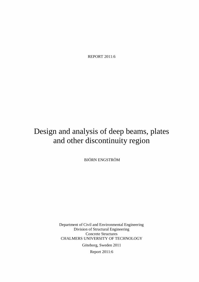
It is generally assumed that normal stresses in a section x of a fully prestressed beam

under service load can be determined by means of Navier’s formula, for instance by

using the tendon force approach.

zxI

xMxexP

xA

xPz

net

i

net

i

c)(

)()()(

)(

)()(

This expression for stress calculations has been derived under the assumption that plane

sections remain plane in bending, and that the materials have a linear elastic response. It

is obvious, however, that stresses near the anchorage of tendons near the end of a post-

tensioned beam can not be linearly distributed across the section. Near the anchorage the

compressive stresses, due to equilibrium conditions, need to be concentrated to the

region just under the anchor plate, see Figure 1. Hence, the stress field is essentially

influenced by the dimension of the anchor plate, which is not at all considered by

Navier’s formula.

D B

zI

MeP

A

Pzc

)(

Figure 1 Stress field in the end of a post-tensioned beam

In the end of the beam these stresses from the anchorage are spread out across the

section within a ‘dispersion zone’. At a certain distance from the anchorage the

conditions are more stable and from this section on Navier’s formula gives a reasonable

estimate of the stress distribution across the section. Within the zone where the

compressive stresses disperse across the section, transverse tensile stresses appear

which, in a concrete structure, might result in cracking. To keep equilibrium and prevent

uncontrolled development of cracks, transverse reinforcement needs to be designed and

provided. The zone where the concentrated force from the anchorage disperses across

the section is referred to as a ‘discontinuity region’.

2

Another example is a column head that supports two beams near the corners, Figure 2.

The column head is subjected to the load from each of the beams. If these loads are

assumed to be the same, equal to Q, and the beams are symmetrically arranged on the

column head, the average compressive stress in the column can be calculated as

hb

Qc

2

Q Q

D

B

b

b

Q2

Figure 2 Column head subjected to loads from supported beams

However, near the top of the column the compressive stresses will be concentrated under

the bearings only. At a certain distance from the top the stresses have evened out across

the section and the actual stress is found to be the same as the average stress. In the

dispersion zone where the concentrated loads are evened out, transverse tensile stresses

appear with risk of cracking and corresponding need for reinforcement.

In a discontinuity region the assumption concerning plane sections remaining plane

under loading is generally not valid. If a region is a discontinuity region or not depends

not only on the geometry and location of the region, but also on the load case. For

instance a column head is a discontinuity zone when it is subjected to concentrated

loads. If the same column head is subjected to a uniformly distributed load q, the top

region of the column will not be a discontinuity region, since in this case plane sections

remain plane under loading. For all sections of the column the stresses can be calculated

as

h

qc

Hence, in the design of reinforced concrete members it is important and appropriate to

distinguish ‘discontinuity regions’ and ‘continuity regions’ Schlaich et al. (1987). In a

discontinuity region the effect of a local discontinuity is evened out. In the adjacent

continuity region, the effect of the same local discontinuity is not noticeable.

3

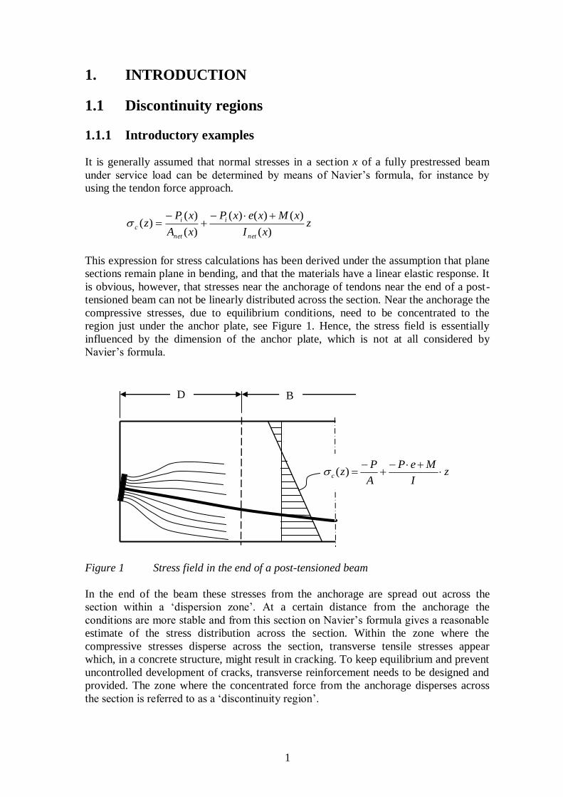
Discontinuity regions can result from geometric discontinuities, Figure 3, or static

discontinuities, Figure 4 Schlaich et al. (1987). Discontinuity regions are also known

as ‘D-regions’ or ‘disturbed’ regions.

In continuity regions plane sections remain plane under loading. Continuity regions are

also known as ‘B-regions’, where the Bernoulli hypothesis of a plane strain distribution

is assumed to be valid.

h

hh

h

h

h1

h1

h1

h2

h2

h2

h2

h1

Figure 3 Discontinuity regions due to geometric discontinuities, adopted from

Scleich et al. (1987)

4

h

h

h

h

h

h

h

h

h2

h

h

Figure 4 Discontinuity regions due to static discontinuities, adopted from Schlaich

et al. (1987)

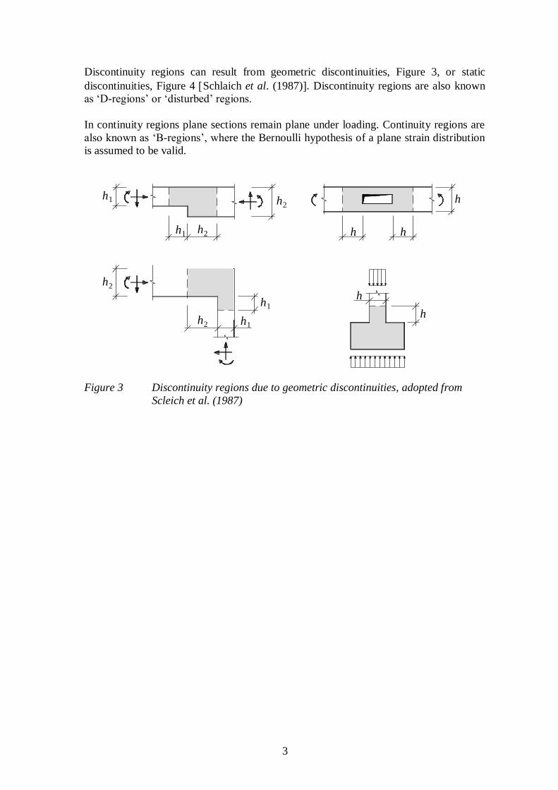
In deep beams the assumption of plane sections remaining plane under loading is often

not valid even in the maximum moment section, Figure 5. The proportions of the

structural member are such that the beam theory cannot be applied in the design. In this

case the whole structural member is a discontinuity region.

5

Figure 5 Distribution of normal strain in a beam and in a deep beam and resulting

forces to corresponding linear elastic stresses

1.1.2 Extension of discontinuity regions

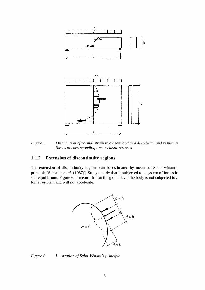
The extension of discontinuity regions can be estimated by means of Saint-Vénant’s

principle Schlaich et al. (1987). Study a body that is subjected to a system of forces in

self equilibrium, Figure 6. It means that on the global level the body is not subjected to a

force resultant and will not accelerate.

h

d h

d h

d h

0

0

Figure 6 Illustration of Saint-Vénant’s principle

6

However, according to Saint-Venant’s principle, stresses will appear in the body as a

local effect of the applied forces and the extension d of the stressed region is equal to the

maximum distance h between the forces in the applied system of forces.

A structural member with a concentrated compressive force F in the centre of the end

section is used to exemplify how the extension of the discontinuity region can be

estimated, Figure 7. Further away in the member, in the continuity region, the strain

distribution is linear, which results in a uniform stress

A

F

The load case with F acting to the right is now divided in two, which, when they are

superimposed, results in the original load case.

h

F

h

Fq

B-zone

h

Fq

F +

D-zone B-zone

0 0

hd

F

D-zone B-zone

hd

Figure 7 Extension of a discontinuity regions determined by Saint-Vénant’s

principle

7

In load case 1 the element is subjected to a uniformly distributed compressive stress =

F/A. In this load case the whole element will be a continuity region with the same stress

in all sections. In load case 2 the beam element is subjected to a force system in self

equilibrium with one centric concentrated force F acting to the right and one uniformly

distributed stress acting to the left. According to Saint-Vénant’s principle stresses will

appear within a region with an extension d equal to the maximum distance between the

forces in the system of self equilibrium. In this case this distance corresponds to the

height h. Outside of this region no stresses appear. When the load cases 1 and 2 are

added, the searched stress field under the concentrated force F is found. Uniformly

distributed stresses appear behind the end zone with extension h. This region deep inside

the member is the ‘continuity zone’. In the region with extension h near the concentrated

force, this uniform stress field is disturbed by local effects. This end region is the

‘discontinuity region’.

According to Eurocode 2 CEN (2004) discontinuity regions ‘extend up to a distance h

from the discontinuity’, where h is the section depth of the member.

However, it is not always that simple to determine the extension of the discontinuity

region. The main principle that should be kept in mind is that the discontinuity region is

the region where the effect of local discontinuities is evened out. For instance near the

end support of a beam with T-section and a wide flange, the effect of the concentrated

support reaction will first be evened out into the web and further on across the width of

the flange. In this case the extension of the discontinuity region will be equal to the

width of the flange, see Figure 8.

b D-zone

B-zone

d b

Figure 8 Extension of discontinuity region of a flanged beam, adopted from

Schlaich (1987)

It is normally not important to define the extension of the discontinuity regions very

accurately. The load path method, presented in Section 2.2 will naturally guide the

designer to a reasonable estimation of the stress field, and by that the discontinuity

region can be defined approximately. The design and arrangement of reinforcement in

the discontinuity region will normally not depend on the exact extension of the zone.

8

1.2 Statically determinate and statically indeterminate

problems

A simply supported beam under load is generally characterised as a statically

determinate problem. This means that the sectional forces can be determined by means

of equilibrium conditions only. This is not the case with a continuous beam on three or

more supports. To solve the sectional forces in such case, equilibrium conditions must

be combined with compatibility conditions and constitutive relations. Constitutive

relations are often depending on assumptions, for instance that there is a linear relation

between moment and curvature in a section. Deep beams can also be classified as

statically determinate and statically indeterminate by the same rules as for ordinary

beams.

When the sectional forces are known in beams or deep beams, the internal stresses are

still unknown. The sectional moment in a statically determinate beam can be resisted in

many different ways depending on the material response in the section. For a given

section, for instance, the internal lever arm will be different if the material has elastic or

plastic response. Furthermore, in a reinforced concrete beam the moment can be resisted

by many alternative combinations of steel area and sectional depth.

Hence, to solve the stress distribution in a section subjected to a bending moment is a

statically indeterminate problem. As usual, this can be solved by a combination of

equilibrium and compatibility conditions and constitutive relations, as exemplified in

Figure 9. For beam sections the assumption of a linear strain distribution (plane sections

remaining plane) is a very convenient compatibility condition, which can be used also in

hand calculations.

x

Vd( x )

d ( x )M

x

s

s s

cc . - 3=3,5 10 ccf

fst

c c( )

ssF = sA

Figure 9 Model to determine the statically indeterminate stress distribution in

a beam section. Equilibrium, compatibility and constitutive relations

are combined.

In deep beams and other discontinuity regions the stress field is statically indeterminate,

independent of if the structural member on the global level is statically determinate or

not. The problem with discontinuity regions is that there exists no simple compatibility

condition which can be used to solve the stress field.

9

1.3 Typical behaviour of discontinuity regions and

modelling

The behaviour of a discontinuity region of reinforced concrete under increasing load can

be characterised by the following four main stages.

Uncracked state

As long as the concrete is uncracked the influence of the reinforcement is small and the

behaviour under load is almost linear. In this state it is appropriate to analyse the

structural member by linear analysis assuming a homogenous material. A linear analysis

will result in a unique stress field (stress field configuration) that is independent of the

load. The stress field can be used to identify regions with high tensile stress that are

prone to cracking and where reinforcement might be needed.

In linear analysis, equilibrium, compatibility and constitutive relations are combined to

solve statically indeterminate problems, for instance stress fields in discontinuity

regions. The constitutive relation is a linear stress-strain relationship for the assumed

homogenous material.

A linear analysis can be carried out by the finite element method – a linear FE analysis.

The stress field can be presented in different ways, stress trajectories, principal stresses,

normal and shear stresses, see Figure 10.

Figure 10 Stress field in deep beam presented by stress trajectories and a

simplified interpretation of it – arch action and need for

reinforcement in the bottom

Typical for a linear analysis is that it results in one unique solution. It means that if the

stress field is determined for one value of the load, the configuration of the stress field

will remain when the load increases (for the same load case). Only the magnitude of the

stresses will increase. Stresses and deformations will increase linearly with the load (for

the same load case). The reason for this linear behaviour is that the stiffness of the

structure is determined by the geometry and the elasticity of the material. The stiffness

will not change when the load increases.

10

A linear analysis requires little information about the structural element. It is often

sufficient with the gross geometry and the load. Any linear elastic material can be

assumed. Therefore, linear analysis can be carried out early in the design process.

Cracked state

When cracking occurs, there will be a drastic change of the stiffness conditions in the

structural member, Figure 11. The stiffness will vary between different regions

depending on if they are cracked or not. Furthermore, the stiffness of the cracked regions

is essentially influenced by the amount and arrangement of the reinforcing steel there.

As a result the configuration of the stress field will deviate from the stress field before

cracking and it will change successively when cracking develops. Even if structural

members have the same geometry and the same load, the stress fields can be different

depending on how the reinforcing steel has been designed and arranged.

The actual stress field depends on the stiffness distribution. In each load step stiffer

regions attract forces from softer regions. Hence, when the load increases and cracking

develops there will be a continuous change of the stiffness distribution and, as a result,

of the stress field configuration. This is known as ‘stress redistribution due to cracking’.

In each load step stresses redistribute, since forces are controlled by the stiffness

distribution that varies continuously.

Figure 11 Deep bream of reinforced concrete in the cracked state

When the configuration of the stress field varies under increasing load, stresses and

deformations will not increase in proportion to the load. Instead there will be a non-

linear behaviour, in spite of the fact that the materials, concrete and steel, still have

linear elastic material responses.

It is not possible to predict the stress field or the behaviour in the cracked state by linear

analysis. Instead non-linear analysis is needed. This can be carried out as a non-linear

FE analysis. For a reinforced concrete member a non-linear analysis considering

cracking of concrete by fracture mechanics, reinforcing steel and the interaction between

steel and concrete is an advanced analysis. It requires full information about the

structural member concerning material properties and reinforcement arrangement and

can only be carried out as verification at the end of the design process when the data is

available.

11

Most reinforced concrete elements will be cracked under service load, but this normal

behaviour is seldom predicted accurately in practice. It is commonly assumed that a

linear analysis can be used to estimate the behaviour in the service state. However, it

should be kept in mind that this is an approximation of the real behaviour. It should also

be noted that a reinforced concrete element will have a non-linear behaviour even if it is

designed on the basis of linear analysis (using a stress field found by linear analysis).

Ultimate state

The ultimate state is characterised by non-linear response of the materials. When one of

the materials, concrete or steel, starts to have a significant non-linear behaviour, the

structural element reaches the ultimate state. A typical event is when the reinforcement

starts to yield in a region of the element. The ultimate state lasts, during load increase,

until the collapse of the structural member (this is the ultimate limit state).

When plastic deformations develop in a region, this is equivalent with a drastic decrease

of, or even loss of, stiffness. Since, in each load step, stiffer regions attract forces from

softening regions, plastic behaviour in a highly stressed region results in stress

redistribution in the structural member and a change of the stress field configuration.

When stress redistribution is caused by plastic deformations, this is known as ‘plastic

redistribution’. Large plastic deformations can result in considerable stress

redistribution. Therefore, the stress field configuration obtained late in the ultimate state,

can deviate considerably from that in the uncracked state.

For instance, when the main tie in the deep beam in Figure 12 starts to yield, the tie loses

stiffness and the deflection starts to increase considerably. Consequently, the cracks

propagate upwards and crack widths increases. As a result the compressive arch will be

forced upwards. Even though the tensile force in the main tie is constant after yielding,

the load on the deep beam can increase since the internal lever arm increases. It means

that the configuration of the stress field changes due to plastic redistribution in the

ultimate state. This can continue as long as there is room enough for the compressive

arch to rise and no critical details limit the load-bearing capacity. The anchorage of the

main tie and the resistance of the highly compressed regions at the supports are critical

issues in the design.

Figure 12 Example of plastic redistribution of stress field of a deep beam in the

ultimate state, a) before, b) after plastic redistribution and critical issues

Loss of

anchorage

in node

Crushing of

compression

node

12

Plastic redistribution results in non-linear behaviour, and as for the cracked state non-

linear analysis is needed to predict the structural response. In this case information about

the non-linear behaviour of the materials is needed.

Ultimate limit state

In the ultimate limit state the structural member is on the limit of collapse. A further

small increase of the load can not be resisted, because there are no reserves left that can

be mobilised by plastic redistribution. Instead, a collapse mechanism develops. In this

stage the plastic resistance is reached in some critical regions that determine the

resistance of the whole structural member.

The final equilibrium condition can be studied by means of theory of plasticity, which

assumes an ideally plastic behaviour of the materials. Such an analysis is known as

‘plastic analysis’. The strut and tie method is a method for plastic analysis, lower bound

approach, see Section 3.1. Strut and tie models are used to simulate stress fields of

cracked reinforced concrete in the ultimate limit state, after considerable plastic

redistribution, Figure 13. The strut and tie method requires little information: gross

geometry, loads, and strength of materials (plastic resistance). It can be used early in the

design process to design and arrange reinforcing steel.

When plastic analysis is used for design and the problem is statically indeterminate,

there exist many alternative solutions. It means that the load in the ultimate limit state

can be carried by many alternative stress fields. One of the alternative models results in

a certain reinforcement arrangement, which in turn results in a certain stiffness

distribution and corresponding development of the stress field. It means that each design

out of possible alternatives results in its own way to carry the load.

Figure 13 Idealisation of the stress field in the ultimate limit state by a strut and

tie model

As mentioned above the behaviour in the ultimate state of a designed structural member

can be analysed by non-linear analysis. When failure is reached in the model, this is

equivalent with the conditions in the ultimate limit state. Hence, the non-linear analysis

can also be used to predict the behaviour and the resistance of a member in the ultimate

limit state.

13

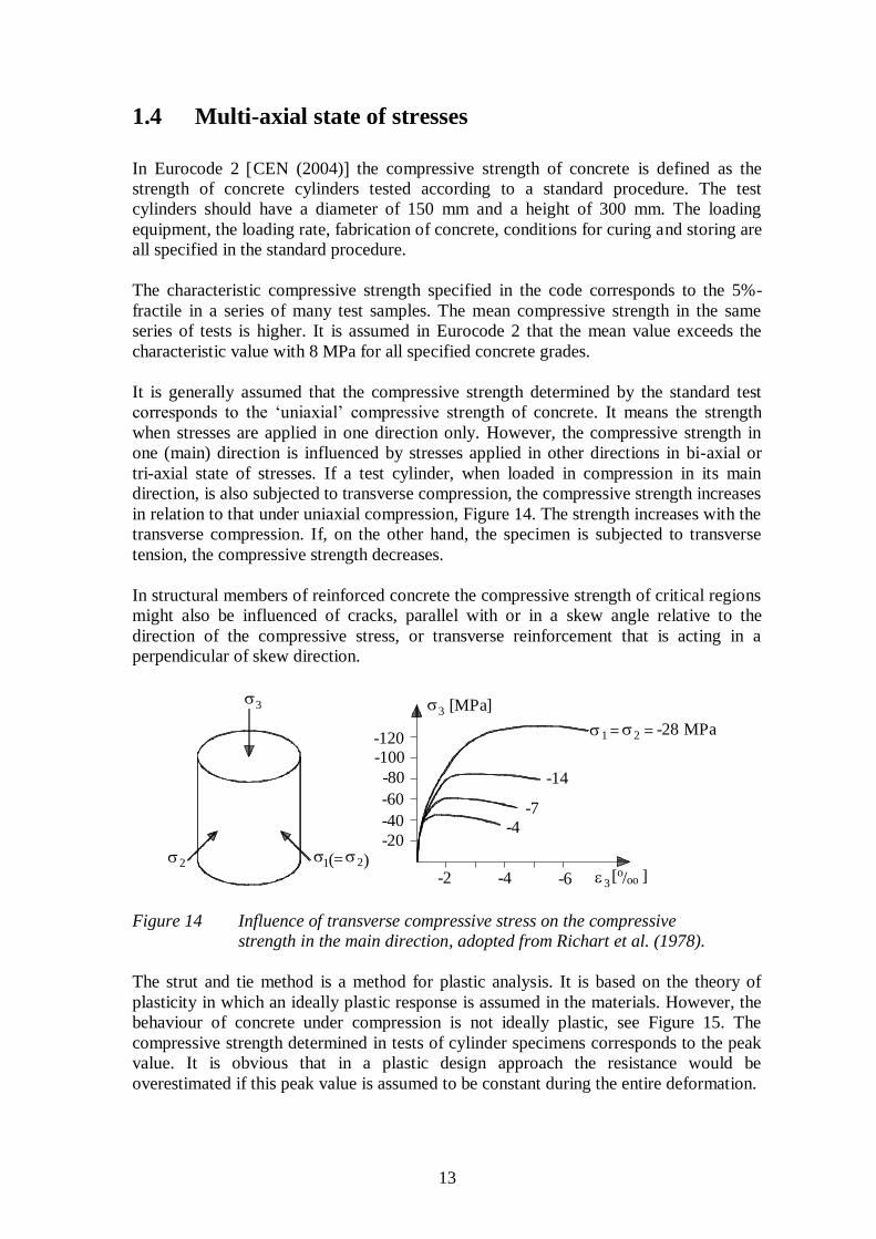
1.4 Multi-axial state of stresses

In Eurocode 2 CEN (2004) the compressive strength of concrete is defined as the

strength of concrete cylinders tested according to a standard procedure. The test

cylinders should have a diameter of 150 mm and a height of 300 mm. The loading

equipment, the loading rate, fabrication of concrete, conditions for curing and storing are

all specified in the standard procedure.

The characteristic compressive strength specified in the code corresponds to the 5%-

fractile in a series of many test samples. The mean compressive strength in the same

series of tests is higher. It is assumed in Eurocode 2 that the mean value exceeds the

characteristic value with 8 MPa for all specified concrete grades.

It is generally assumed that the compressive strength determined by the standard test

corresponds to the ‘uniaxial’ compressive strength of concrete. It means the strength

when stresses are applied in one direction only. However, the compressive strength in

one (main) direction is influenced by stresses applied in other directions in bi-axial or

tri-axial state of stresses. If a test cylinder, when loaded in compression in its main

direction, is also subjected to transverse compression, the compressive strength increases

in relation to that under uniaxial compression, Figure 14. The strength increases with the

transverse compression. If, on the other hand, the specimen is subjected to transverse

tension, the compressive strength decreases.

In structural members of reinforced concrete the compressive strength of critical regions

might also be influenced of cracks, parallel with or in a skew angle relative to the

direction of the compressive stress, or transverse reinforcement that is acting in a

perpendicular of skew direction.

-120-100

-80

-60

-40

-20

-2 -4 -6

3 [MPa]3

22 (= )

1 2= = -28 MPa

-14

[ ]ooo/

-7-4

3

1

Figure 14 Influence of transverse compressive stress on the compressive

strength in the main direction, adopted from Richart et al. (1978).

The strut and tie method is a method for plastic analysis. It is based on the theory of

plasticity in which an ideally plastic response is assumed in the materials. However, the

behaviour of concrete under compression is not ideally plastic, see Figure 15. The

compressive strength determined in tests of cylinder specimens corresponds to the peak

value. It is obvious that in a plastic design approach the resistance would be

overestimated if this peak value is assumed to be constant during the entire deformation.

14

20

40

60

80

0,001 0,002 0,003 0,004 cc

cc [ MPa ]

Figure 15 Stress-strain relationship for concrete under uniaxial compression.

Various strength classes, adopted from Nilson (1987)

It is reasonable to assume that an equivalent plastic strength, constant during

deformation, must be smaller than the peak value. An effectiveness factor can be used to

relate the equivalent plastic strength to the maximum stress (peak value in standard test).

ccplc ff ,

where fc,pl = equivalent plastic strength to be used in plastic analysis

= effectiveness factor

fcc = uniaxial compressive strength from cylinder test

The effectiveness factor cannot be determined easily, but varies for different types of

structural problems, Nielsen (1984). Eurocode 2 gives expressions for estimation of the

effectiveness factor for some fundamental cases.

In the strut and tie method, the resistance of the member depends among others on the

compressive strength of concrete in struts and nodes. Of the reasons mentioned above

the design compressive strength of these components must be determined with due

regard to the actual state of stresses. This is further discussed in Sections 2.4.6 and 2.4.7,

where recommendations from Eurocode 2 are presented.

15

2. THE STRUT AND TIE METHOD

The following presentation of the strut and tie method is based on the concept which

was developed by Schlaich and co-workers. An extensive presentation of the method

was given by Schlaich et al. (1987). At that time the method was considered for the new

CEB-FIP Model Code, which was under preparation. A more detailed presentation of

the method was given in the German Concrete Design Handbook Schlaich and Schäfer

(1989), and a concise presentation is found in Schlaich and Schäfer (1991). In the CEB-

FIP Model Code 1990 CEB-FIP (1993) the method using stress fields with struts,

nodes and ties was possible to use for structural analysis and design of deep beams and

discontinuity regions. A text book on design according to Model Code 1990 was

published as fib bulletins (International Federation for Structural Concrete), where two

sections were devoted to design of nodes and design of deep beams and discontinuity

regions Schäfer (1999a) and (1999b). Later on the strut and tie method has been

introduced in Eurocode 2 CEN (2004).

2.1 Procedure

The strut and tie method is based on theory of plasticity. The purpose of the strut and tie

model is to simulate the stress field in cracked reinforced concrete in the ultimate limit

state. Then the structure is just about to reach collapse and there has been more or less

plastic redistribution. In critical regions the materials have reached plastic behaviour.

Nevertheless, it is normally recommended to choose a strut and tie model that reminds,

in a simplified way, of the linear elastic stress field. The reasons are

limited ability to plastic redistribution in reinforced concrete;

the design should also fulfil needs concerning appropriate performance in the

service state.

These items are further discussed in Section 3.2. However, it should be noticed that the

linear elastic stress field should not be considered as the ‘true’ solution, which should be

copied by the strut and tie model. This is not at all the case. It is generally

recommended, however, that the stress field in the ultimate limit state after cracking and

yielding is not too ‘extreme’ and too different from the stress-field before cracking and

yielding.

To get an appropriate strut and tie model that reminds, in a simplified way, of the linear

elastic stress fields there are two possible approaches. The model can be developed on

the basis of:

the load path method, Section 2.2, together with application rules for the

geometry of the strut and tie model, Section 2.3.1.

stress trajectories or principal stresses from a linear FE analysis

When a structural element is designed using the strut and tie method, it is appropriate to

carry out the calculations according to the following steps.

1) Structural analysis is carried out to solve support reactions and sectional forces

under the design load, Figure 16. For statically indeterminate problems an

appropriate choice of unknown has to be done.

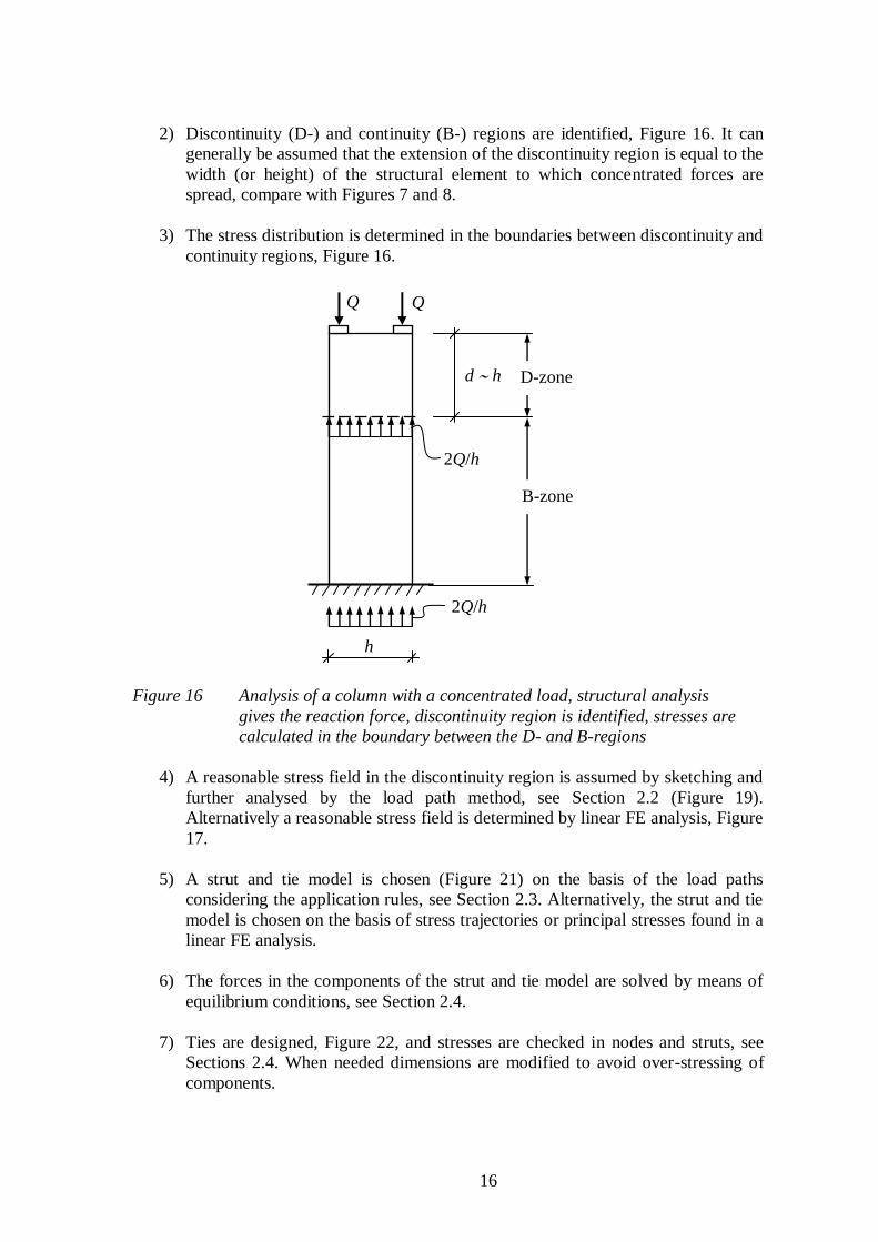
16

2) Discontinuity (D-) and continuity (B-) regions are identified, Figure 16. It can

generally be assumed that the extension of the discontinuity region is equal to the

width (or height) of the structural element to which concentrated forces are

spread, compare with Figures 7 and 8.

3) The stress distribution is determined in the boundaries between discontinuity and

continuity regions, Figure 16.

h

2Q/h

2Q/h

Q Q

d h

B-zone

D-zone

Figure 16 Analysis of a column with a concentrated load, structural analysis

gives the reaction force, discontinuity region is identified, stresses are

calculated in the boundary between the D- and B-regions

4) A reasonable stress field in the discontinuity region is assumed by sketching and

further analysed by the load path method, see Section 2.2 (Figure 19).

Alternatively a reasonable stress field is determined by linear FE analysis, Figure

17.

5) A strut and tie model is chosen (Figure 21) on the basis of the load paths

considering the application rules, see Section 2.3. Alternatively, the strut and tie

model is chosen on the basis of stress trajectories or principal stresses found in a

linear FE analysis.

6) The forces in the components of the strut and tie model are solved by means of

equilibrium conditions, see Section 2.4.

7) Ties are designed, Figure 22, and stresses are checked in nodes and struts, see

Sections 2.4. When needed dimensions are modified to avoid over-stressing of

components.

17

Figure 17 Strut and tie model developed on the basis of stress trajectories from

a linear analysis, idea from Schlaich et al. (1987)

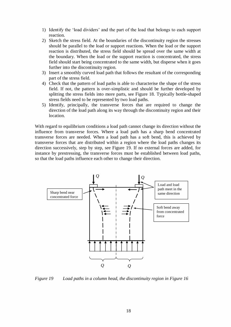
2.2 The load path method

In the load path method, streamlined load paths are inserted to simulate the stress field in

a simplified way. The load path should in every section along its way represent the

resultant of the corresponding stress field. It is often appropriate to divide a stress field

in several parts and introduce a load path in each of them. Otherwise, the model could be

over-simplistic and not guide the designer to an appropriate design and detailing, see

Figure 18.

For a given load case there is a unique relation between the load applied on the structure

and the support reactions. It means that each support reaction is caused by a certain part

of the load. The load is divided by ‘load-dividers’ in sections where the shear force is

zero, so that each part of the load is carried by the nearest support, Figure 18.

RA RB RA RB2 RB1

Figure 18 Stress field and load paths in a deep beam with cantilevering end,

a) over-simplistic model with two load paths, b) appropriate model

with three load paths

In the load path method a smoothly curved force path is inserted between the support

reaction and that part of the load that causes this reaction. When necessary, in order to

simulate the stress fields better, support reactions are split in two or more parts. It is

appropriate to develop the load paths according to the following steps.

18

1) Identify the ‘load dividers’ and the part of the load that belongs to each support

reaction.

2) Sketch the stress field. At the boundaries of the discontinuity region the stresses

should be parallel to the load or support reactions. When the load or the support

reaction is distributed, the stress field should be spread over the same width at

the boundary. When the load or the support reaction is concentrated, the stress

field should start being concentrated to the same width, but disperse when it goes

further into the discontinuity region.

3) Insert a smoothly curved load path that follows the resultant of the corresponding

part of the stress field.

4) Check that the pattern of load paths is able to characterise the shape of the stress

field. If not, the pattern is over-simplistic and should be further developed by

splitting the stress fields into more parts, see Figure 18. Typically bottle-shaped

stress fields need to be represented by two load paths.

5) Identify, principally, the transverse forces that are required to change the

direction of the load path along its way through the discontinuity region and their

location.

With regard to equilibrium conditions a load path cannot change its direction without the

influence from transverse forces. Where a load path has a sharp bend concentrated

transverse forces are needed. When a load path has a soft bend, this is achieved by

transverse forces that are distributed within a region where the load paths changes its

direction successively, step by step, see Figure 19. If no external forces are added, for

instance by prestressing, the transverse forces must be established between load paths,

so that the load paths influence each other to change their direction.

Q Q

Q Q

Load and load

path meet in the

same direction

Soft bend away

from concentrated

force

Sharp bend near

concentrated force

Figure 19 Load paths in a column head, the discontinuity region in Figure 16

19

In the load path method the load paths should fulfil the following rules:

The load path should in each section along its way represent the resultant of the

stress field which it simulated.

Load paths cannot cross each other.

At the boundary of the discontinuity region the load path should start in the same

direction as the load or support reaction.

Load paths should have a sharp bend near a concentrated force.

When a load path needs to change direction away from a concentrated force the

bend should be soft.

In certain cases there will be no complete balance between loads and support reactions

when load paths are inserted according to the principles listed above. In such cases a

load path in ‘U-turn’ must be added. A load path in ‘U-turn’ enters and leaves the

discontinuity region at the same boundary on the ‘reaction side’, see Figure 20.

D D B

T

T

Q Q

T

T

Q Q

Figure 20 Example of load path in U-turn. Post-tensioned beam with eccentric

anchorage

20

2.3 Development of the strut and tie model

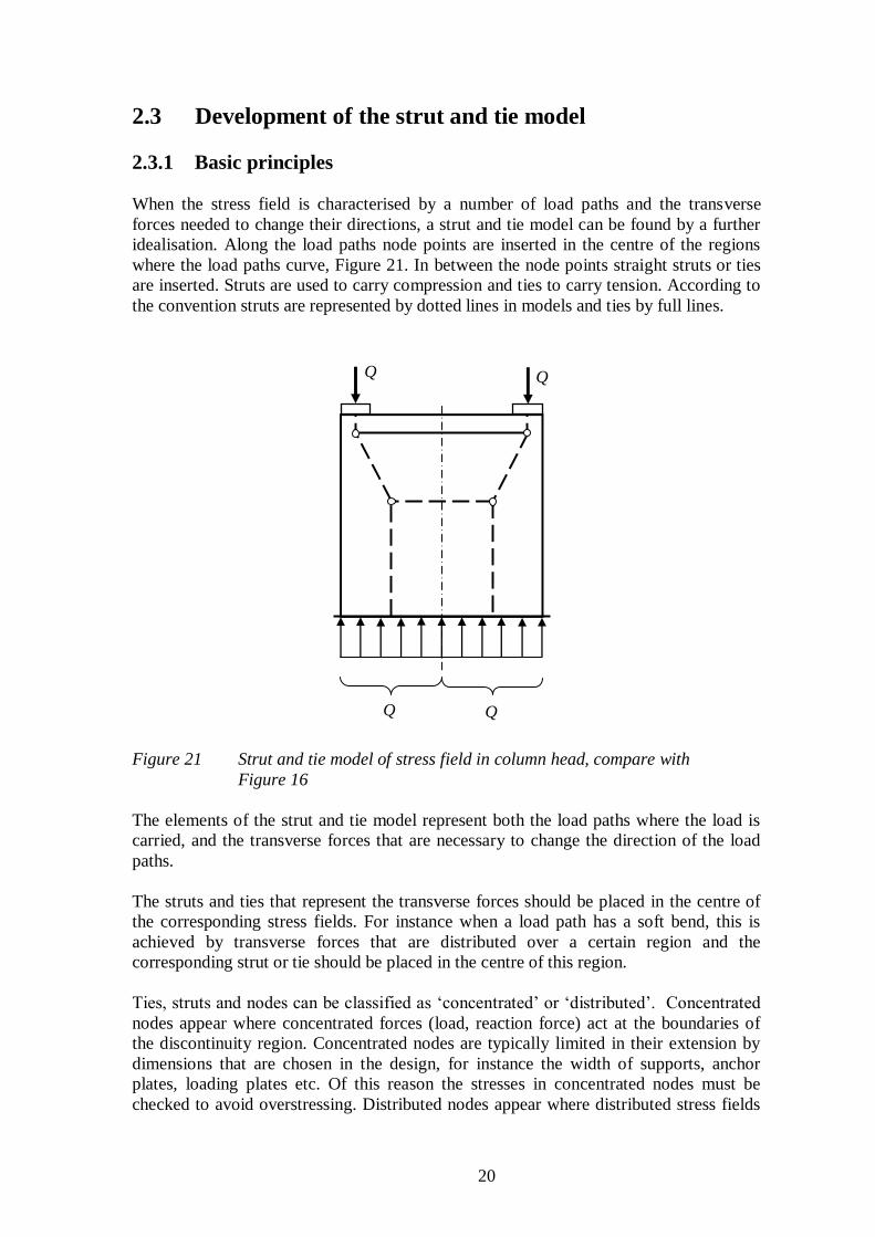
2.3.1 Basic principles

When the stress field is characterised by a number of load paths and the transverse

forces needed to change their directions, a strut and tie model can be found by a further

idealisation. Along the load paths node points are inserted in the centre of the regions

where the load paths curve, Figure 21. In between the node points straight struts or ties

are inserted. Struts are used to carry compression and ties to carry tension. According to

the convention struts are represented by dotted lines in models and ties by full lines.

Q Q

Q Q

Figure 21 Strut and tie model of stress field in column head, compare with

Figure 16

The elements of the strut and tie model represent both the load paths where the load is

carried, and the transverse forces that are necessary to change the direction of the load

paths.

The struts and ties that represent the transverse forces should be placed in the centre of

the corresponding stress fields. For instance when a load path has a soft bend, this is

achieved by transverse forces that are distributed over a certain region and the

corresponding strut or tie should be placed in the centre of this region.

Ties, struts and nodes can be classified as ‘concentrated’ or ‘distributed’. Concentrated

nodes appear where concentrated forces (load, reaction force) act at the boundaries of

the discontinuity region. Concentrated nodes are typically limited in their extension by

dimensions that are chosen in the design, for instance the width of supports, anchor

plates, loading plates etc. Of this reason the stresses in concentrated nodes must be

checked to avoid overstressing. Distributed nodes appear where distributed stress fields

21

meet. A distributed stress field can be the result of a distributed load or reaction at a

boundary or distributed transverse forces needed to softly change the direction of a load

path away from concentrated forces. It is not necessary to check stresses in distributed

nodes, because there is no limitation of their dimensions. A distributed node cannot be

overstressed. Instead, by means of plastic redistribution, the structure will incorporate

more and more volume of material into the node, if it becomes highly stressed.

A tie which is needed in a concentrated node to abruptly change the direction of load

path is a concentrated tie. This should be designed by reinforcement concentrated

together near the edge of the element, see Figure 22. Typical examples are ties in deep

beams, to enable ‘tied arch action’, or the tensile chord in beams. When a wide

transverse tensile stress field is needed to softly change the direction of a load path, this

is achieved by a distributed tie. A distributed tie should be designed by reinforcement

that is distributed on many small diameter bars, which are placed within the

corresponding region.

Figure 22 Reinforcement for concentrated tie in column head, compare with

Figure 21

When a transverse strut between concentrated nodes is needed to change the direction of

load paths, this can be a concentrated strut that follows the edge of the element. A

compressive zone of a beam is a typically example. Otherwise, concentrated struts will

not pass through the interior of a discontinuity region. It is natural that concentrated

forces will spread out transversally and incorporate more and more of the material

available. This spread of compressive stresses from a concentrated node can be ‘fan-

shaped’ or ‘bottle-shaped’.

It should be checked early in the development of the strut and tie model, before

calculations are carried out, that the model is able to fulfil equilibrium conditions. By a

visual inspection of the nodes the conditions for obtaining horizontal and vertical

equilibrium can be checked and major mistakes can be revealed.

22

To achieve a model with perfect equilibrium, the nodes should be positioned carefully

with regard to the locations of reaction forces. When a stress field has been divided in

parts, each part is represented by one load path. The load path should meet its reaction in

the centre of the corresponding stress field, see Figure 23. This means that support

reactions in supports with several load paths must be divided in parts proportional to the

respective loads and the node should be in the centre of each part.

RA RB2 RB1 RB1 RB2

lB1 lB2

lB

B

B

B1B1 l

R

Rl

B

B

B2B2 l

R

Rl

B2B1B RRR

Figure 23 Support regions should be divided in proportion to the load paths

before node points are inserted in the centre of the respective stress

field

In the development of a strut and tie model one or more angles between struts and ties

need to be chosen. It is important to be aware of the number of possible choices that can

be made. When one or some angles are chosen, other angles in the model will be

determined and can be solved. They cannot be chosen too. If possible the angles

between struts and ties should be close to preferred values, see Section 2.3.2.

2.3.2 Application rules

With regard to the need for ductility and an appropriate behaviour in the service state,

see Section 3.3, it is recommended to follow the following application rules.

Stresses under concentrated forces (loads, reactions) should be spread out as

soon as possible when they enter the discontinuity region. A deviation angle of

about 30 is a reasonable choice and it should not exceed 45, Figure 24.

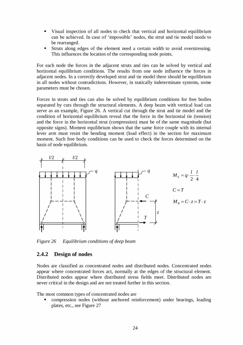
The angle between a strut and a tie should not be too small, Figure 25.

o In case of a strut meeting a single tie the preferred angle is about 60 and

it should not be less than 45.

o In case of a strut between two perpendicular ties the preferred angle is

about 45 and it should not be less than 30.

Concentrated forces should not be carried by concentrated struts across wide

elements, with exception for concentrated compressive zones in continuity

regions (B-regions).

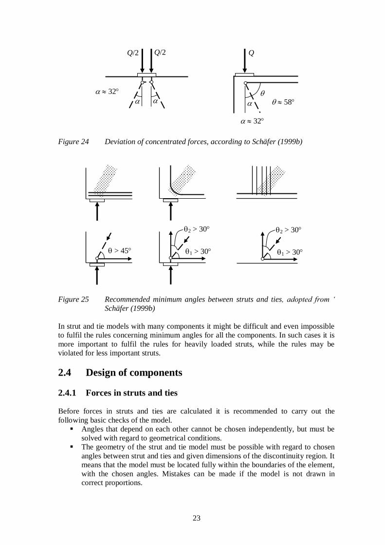
23

32

Q/2 Q/2 Q

32

58

Figure 24 Deviation of concentrated forces, according to Schäfer (1999b)

> 45 1 > 30

2 > 30

1 > 30

2 > 30

Figure 25 Recommended minimum angles between struts and ties, adopted from ‘

Schäfer (1999b)

In strut and tie models with many components it might be difficult and even impossible

to fulfil the rules concerning minimum angles for all the components. In such cases it is

more important to fulfil the rules for heavily loaded struts, while the rules may be

violated for less important struts.

2.4 Design of components

2.4.1 Forces in struts and ties

Before forces in struts and ties are calculated it is recommended to carry out the

following basic checks of the model.

Angles that depend on each other cannot be chosen independently, but must be

solved with regard to geometrical conditions.

The geometry of the strut and tie model must be possible with regard to chosen

angles between strut and ties and given dimensions of the discontinuity region. It

means that the model must be located fully within the boundaries of the element,

with the chosen angles. Mistakes can be made if the model is not drawn in

correct proportions.

24

Visual inspection of all nodes to check that vertical and horizontal equilibrium

can be achieved. In case of ‘impossible’ nodes, the strut and tie model needs to

be rearranged.

Struts along edges of the element need a certain width to avoid overstressing.

This influences the location of the corresponding node points.

For each node the forces in the adjacent struts and ties can be solved by vertical and

horizontal equilibrium conditions. The results from one node influence the forces in

adjacent nodes. In a correctly developed strut and tie model there should be equilibrium

in all nodes without contradictions. However, in statically indeterminate systems, some

parameters must be chosen.

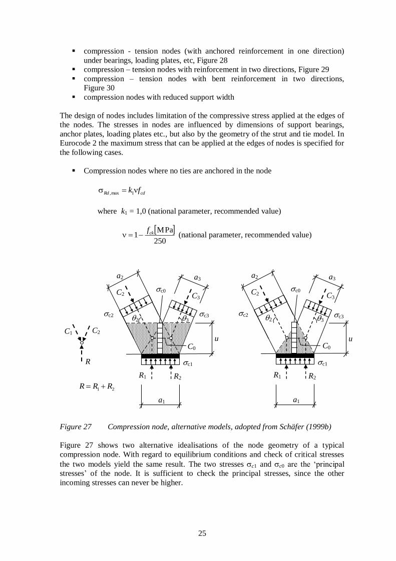
Forces in struts and ties can also be solved by equilibrium conditions for free bodies

separated by cuts through the structural elements. A deep beam with vertical load can

serve as an example, Figure 26. A vertical cut through the strut and tie model and the

condition of horizontal equilibrium reveal that the force in the horizontal tie (tension)

and the force in the horizontal strut (compression) must be of the same magnitude (but

opposite signs). Moment equilibrium shows that the same force couple with its internal

lever arm must resist the bending moment (load effect) in the section for maximum

moment. Such free body conditions can be used to check the forces determined on the

basis of node equilibrium.

l/2 l/2

q q

C

T z

42

llqM E

TC

zTzCMR

Figure 26 Equilibrium conditions of deep beam

2.4.2 Design of nodes

Nodes are classified as concentrated nodes and distributed nodes. Concentrated nodes

appear where concentrated forces act, normally at the edges of the structural element.

Distributed nodes appear where distributed stress fields meet. Distributed nodes are

never critical in the design and are not treated further in this section.

The most common types of concentrated nodes are

compression nodes (without anchored reinforcement) under bearings, loading

plates, etc., see Figure 27

25

compression - tension nodes (with anchored reinforcement in one direction)

under bearings, loading plates, etc, Figure 28

compression – tension nodes with reinforcement in two directions, Figure 29

compression – tension nodes with bent reinforcement in two directions,

Figure 30

compression nodes with reduced support width

The design of nodes includes limitation of the compressive stress applied at the edges of

the nodes. The stresses in nodes are influenced by dimensions of support bearings,

anchor plates, loading plates etc., but also by the geometry of the strut and tie model. In

Eurocode 2 the maximum stress that can be applied at the edges of nodes is specified for

the following cases.

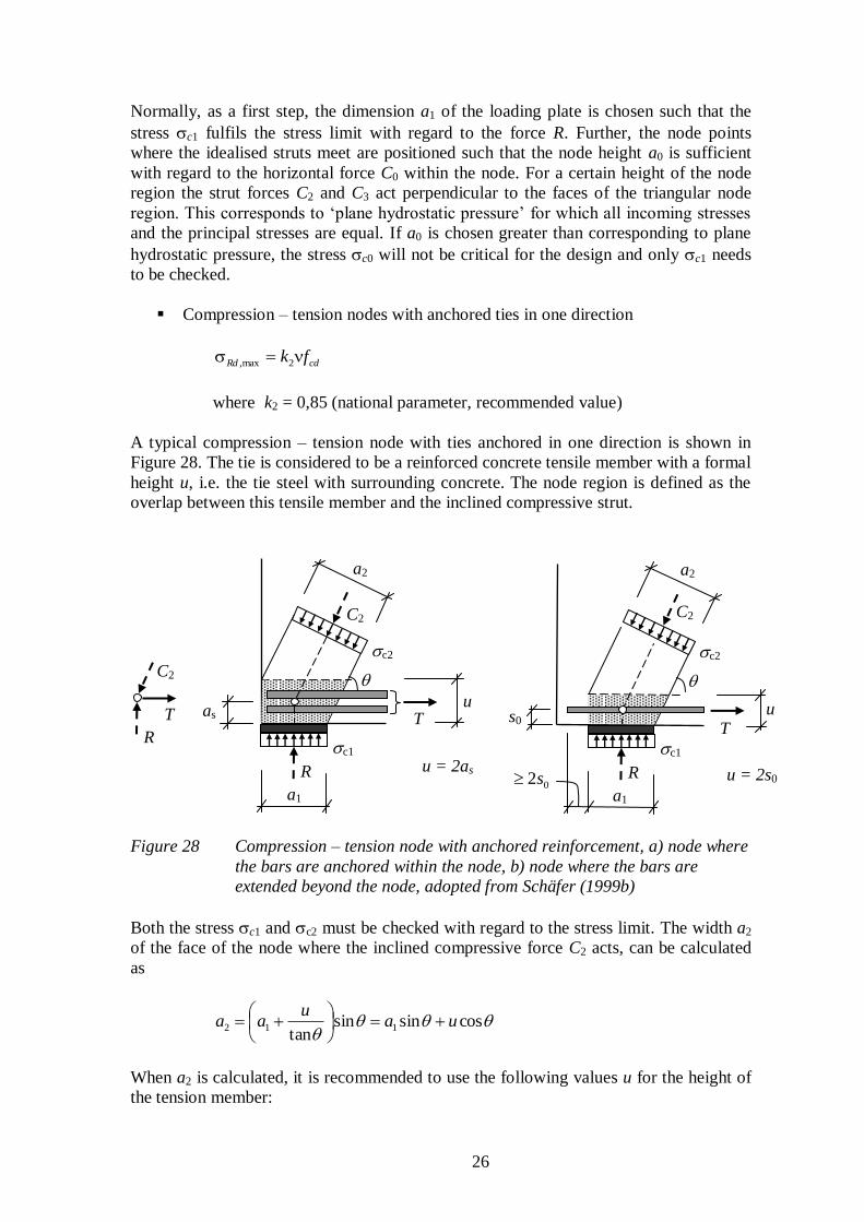
Compression nodes where no ties are anchored in the node

cdRd fk 1max,

where k1 = 1,0 (national parameter, recommended value)

250

MPa1 ckf (national parameter, recommended value)

c1

R1 R2

C2 C3 c0

c3 c2 2 3

a1

u

a3 a2

R

C2 C1

c1

R1 R2

C2 C3 c0

c3 c2 2 3

a1

u

a3 a2

21 RRR

C0 C0

Figure 27 Compression node, alternative models, adopted from Schäfer (1999b)

Figure 27 shows two alternative idealisations of the node geometry of a typical

compression node. With regard to equilibrium conditions and check of critical stresses

the two models yield the same result. The two stresses c1 and c0 are the ‘principal

stresses’ of the node. It is sufficient to check the principal stresses, since the other

incoming stresses can never be higher.

26

Normally, as a first step, the dimension a1 of the loading plate is chosen such that the

stress c1 fulfils the stress limit with regard to the force R. Further, the node points

where the idealised struts meet are positioned such that the node height a0 is sufficient

with regard to the horizontal force C0 within the node. For a certain height of the node

region the strut forces C2 and C3 act perpendicular to the faces of the triangular node

region. This corresponds to ‘plane hydrostatic pressure’ for which all incoming stresses

and the principal stresses are equal. If a0 is chosen greater than corresponding to plane

hydrostatic pressure, the stress c0 will not be critical for the design and only c1 needs

to be checked.

Compression – tension nodes with anchored ties in one direction

cdRd fk 2max,


A typical compression – tension node with ties anchored in one direction is shown in

Figure 28. The tie is considered to be a reinforced concrete tensile member with a formal

height u, i.e. the tie steel with surrounding concrete. The node region is defined as the

overlap between this tensile member and the inclined compressive strut.

u = 2as

C2

T

R c1

R

T

C2

c2

a2

a1

as

c1

R

T

C2

c2

a2

a1

s0

u = 2s0 02s

u u

Figure 28 Compression – tension node with anchored reinforcement, a) node where

the bars are anchored within the node, b) node where the bars are

extended beyond the node, adopted from Schäfer (1999b)

Both the stress c1 and c2 must be checked with regard to the stress limit. The width a2

of the face of the node where the inclined compressive force C2 acts, can be calculated

as

cossinsintan

112 uau

aa

When a2 is calculated, it is recommended to use the following values u for the height of

the tension member:

27

0u for nodes with one layer of reinforcement not extending

beyond the node region Schäfer(1999b)

02su for nodes with one layer of reinforcement extending at least the

distance 2s0 beyond the node region Eurocode 2

snsu 12 0

for nodes with n layers of reinforcement extending at least the

distance 2s0 beyond the node region Eurocode 2

where s0 = distance from the bottom edge to the centre of the bottom

reinforcement layer

s = spacing between reinforcement layers (centre to centre)

The design of the node includes normally the following steps

Choice of support length a1 such that the stress limit is fulfilled with regard to

the force R

Arrangement of reinforcement in one or several layers

Check of concrete stress in section a2 with regard to the force C2

Arrangement of anchorage of the tie bars, see Section 2.4.4

Provision of transverse reinforcement in the anchorage and node regions

Proper detailing of compression – tension nodes is very important. The anchorage of the

tie bars results in splitting effects and micro cracking. Transverse reinforcement, in form

of stirrups or U-bends around the anchored bars, confines the anchorage zone and

balances splitting effects. Furthermore, it is favourable if some longitudinal compression

is built up beyond the node region to confine it by compression. Therefore, it is

recommended that the tie bars should extend at least a minimum distance 2s0 beyond the

node region, even when it is not required with regard to anchorage (see Section 2.4.4).

If the tie bars are not well distributed across the width of the section transverse tensile

stresses might develop in the anchorage region. Also for this reason transverse

reinforcement is recommended.

For the design of compression – tension nodes it is favourable to keep the angles

between struts and ties greater than 55, arrange the ties in several layers, anchor the

reinforcement to a considerable part behind the node, confine the node region by

stirrups, bearing details and/or friction. Eurocode 2 CEN (2004) permits higher stress

limits in case of improved detailing.

Compression – tension nodes with anchored ties in more than one direction

cdRd fk 3max,


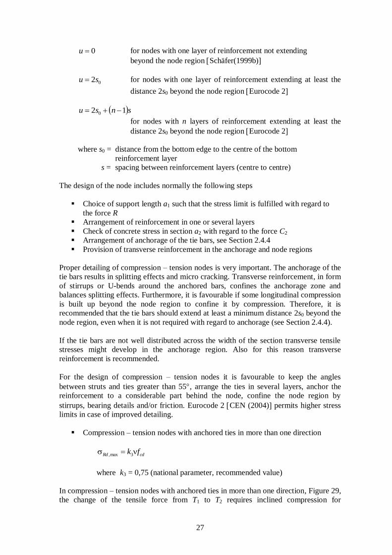
In compression – tension nodes with anchored ties in more than one direction, Figure 29,

the change of the tensile force from T1 to T2 requires inclined compression for

28

equilibrium. The width of the inclined compressive strut depends on the design

anchorage length lbd which is used to anchor the difference between T1 and T2.

C

T1 T1

cc

a

lbd

u = 2s0

u T2

T3

T2

C

T3

Figure 29 Compression – tension node with reinforcement in two directions,

adopted form Schäfer (1999b)

The design of the node regions consists of the following steps.

Arrangement of anchorage for the main reinforcement

Check of stress limit in section a for the compressive force C

Arrangement of the reinforcement for T3, normally loops, hooks or stirrups of

small bars

Arrangement of transverse reinforcement (third direction), normally legs of

stirrups of loops.

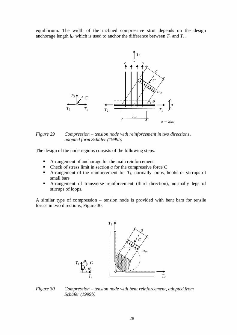
A similar type of compression – tension node is provided with bent bars for tensile

forces in two directions, Figure 30.

C

T2 T2

cc

2

a

T1

C

T1

1

Figure 30 Compression – tension node with bent reinforcement, adopted from

Schäfer (1999b)

29

In this case the width of the strut can be estimated as

sinmda

where = the smaller angle of 1 and 2

dm = mandrel diameter used for forming the bar to the bent shape

2.4.3 Design of ties

In general the tensile force in ties should be resisted by reinforcing steel that is arranged

and anchored in the structural element so that the intended equilibrium system can be

obtained. The reinforcement bars should have the same direction as the tie in the model,

and the gravity centre of the considered group of bars should have the same location as

the tie in the model. The required steel area is determined as

yd

sf

TA

where T = tensile force in tie

fyd = design tensile strength of reinforcing steel

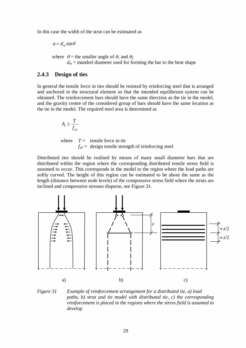
Distributed ties should be realised by means of many small diameter bars that are

distributed within the region where the corresponding distributed tensile stress field is

assumed to occur. This corresponds in the model to the region where the load paths are

softly curved. The height of this region can be estimated to be about the same as the

length (distance between node levels) of the compressive stress field where the struts are

inclined and compressive stresses disperse, see Figure 31.

z z/2

z/2

a) b) c)

Figure 31 Example of reinforcement arrangement for a distributed tie, a) load

paths, b) strut and tie model with distributed tie, c) the corresponding

reinforcement is placed in the regions where the stress field is assumed to

develop

30

Reinforcement that is needed to change the direction of a stress field must be extended

across the full width of this stress field as shown in figure 31. It is not sufficient to locate

the reinforcement just between the node points in the model. The nodes represent the

place where resultants meet, but all components of the vertical stress field a need

transverse tensile force to change its direction from inclined to vertical.

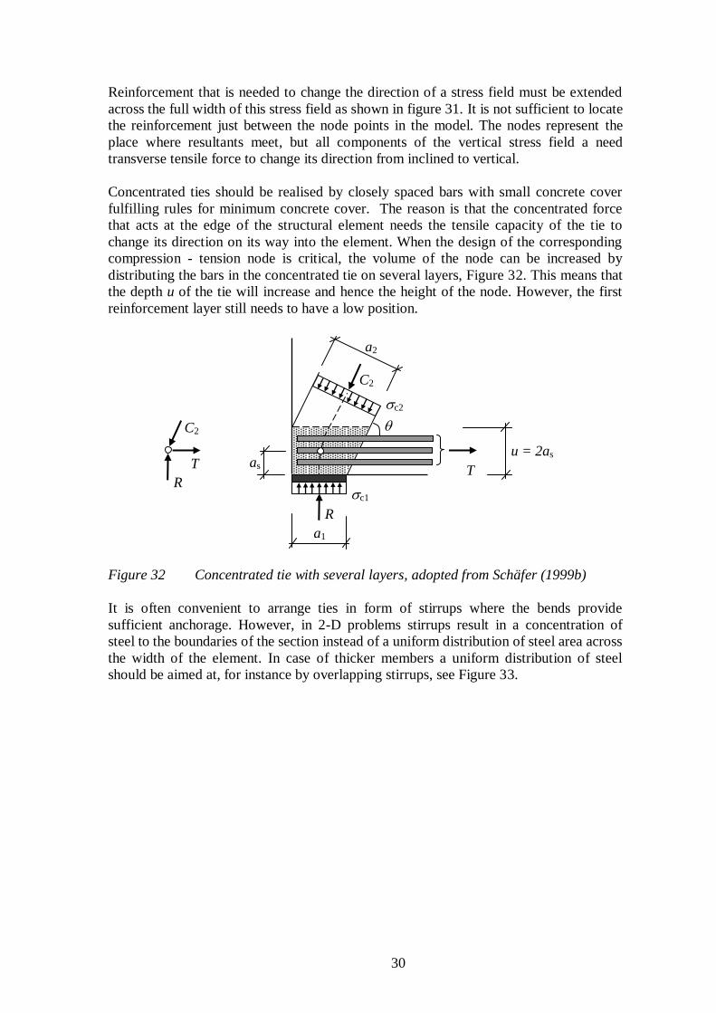
Concentrated ties should be realised by closely spaced bars with small concrete cover

fulfilling rules for minimum concrete cover. The reason is that the concentrated force

that acts at the edge of the structural element needs the tensile capacity of the tie to

change its direction on its way into the element. When the design of the corresponding

compression - tension node is critical, the volume of the node can be increased by

distributing the bars in the concentrated tie on several layers, Figure 32. This means that

the depth u of the tie will increase and hence the height of the node. However, the first

reinforcement layer still needs to have a low position.

c1

R

T

C2

c2

a2

u = 2as

a1

as

C2

T

R

Figure 32 Concentrated tie with several layers, adopted from Schäfer (1999b)

It is often convenient to arrange ties in form of stirrups where the bends provide

sufficient anchorage. However, in 2-D problems stirrups result in a concentration of

steel to the boundaries of the section instead of a uniform distribution of steel area across

the width of the element. In case of thicker members a uniform distribution of steel

should be aimed at, for instance by overlapping stirrups, see Figure 33.

31

h h h

b

b

Figure 33 In wide elements designed by means of 2-D models it is appropriate to

distribute the ties across the width of the member. This can be achieved

by overlapping stirrups

2.4.4 Anchorage of ties

Concentrated ties should be well anchored in the corresponding concentrated nodes. The

compressive force that turns into a new direction in the node is the resultant to a stress

field consisting of many small force components. Each component needs a small

transverse tensile force to change its direction when it passes the node, see Figure 34.

This is achieved by bond stresses that develop along the anchored tie bar. The force in

the tie starts to decrease when the direction of the first force component is influenced.

The tie force decreases successively along the bar when more and more force

components are influenced. In order to change the direction of all force components, the

tie must at least go through the whole stress field.

Figure 34 All force components need a transverse tensile force to change the

direction

The design of the anchorage follows the ordinary rules for bond and anchorage in the

Eurocode 2. The ordinary anchorage length lbd is calculated and compared with the

actual dimensions.

If the calculated anchorage length lbd is shorter than the width a of the node

(compressive stress field), the tie should be extended to the full width of the

node, Figure 35a.

32

If the calculated anchorage length lbd exceeds the width a of the node, the tie

should be anchored with the length lbd behind the section where the tie enters the

node, Figure 35b.

If there is no room for sufficient anchorage behind the node, full anchorage must

be provided by bends, hooks or anchor devices.

When distributed ties are arranged and anchored, it is not sufficient to bring them to the

node point in the strut and tie model, but they must be extended across the whole stress

field that should be deviated. All force components in this stress field need the tensile

force in the tie to change their direction.

a a

lbd

Figure 35 Anchorage of tie in a node region, a) minimum anchorage,

b) anchorage when the calculated anchorage length lbd exceeds the

width of the node

The design on the basis of strut and tie models assumes that the full capacity of ties can

be used in all sections between the nodes. Consequently, sufficient anchorage capacity

to resist the yield load of the ties must be provided in or behind the nodes. In many cases

there is no room for ordinary anchorage lengths, but anchorage must be provided by bent

bars. Very often solutions with closed stirrups are appropriate. A typical example is

shown in Figures 21 and 22. In this case it would not be possible to arrange

reinforcement in form of straight bars.

2.4.5 Stress limitations in struts

The compressive stress in concrete struts should be limited with regard to unfavourable

multi-axial effects. In Eurocode 2 the following two cases are distinguished.

Transverse compression or no transverse stress

For a concrete strut in a region with transverse compressive stress or no transverse stress

the design stress may be calculated as

cdRd fmax, c

ckcccd

ff

where fcd = design compressive strength of concrete

cc = 1,0 (national parameter, recommended value) coefficient

considering long term effects

c = 1,5 (partial factor for concrete in ordinary situations)

33

This means that the strength of the strut is assumed to be the same as for concrete under

uniaxial compression. A typical example is the prismatic stress field of the compressive

zone along an edge of a B-region.

Where multi-axial compression exists, higher design strength could be considered.

However, the third dimension in two-dimensional structures must not be forgotten.

Cracked regions and/or transverse tension

For a concrete strut in a cracked compression zone the design strength should be reduced

and may be calculated as

cdRd f 6,0max,

where 250

MPa1 ckf (national parameter, recommended value)

Transverse tension has a negative effect on the compressive strength. However, it is

normally not necessary to check the stresses of struts provided that the stresses at the

faces of the nodes fulfil the stress limits of the nodes and that the strut is provided with

transverse reinforcement that keeps the strut together in the transverse direction. It is

assumed that the nodes themselves are the critical regions of the stress fields

Schäfer(1999a).

This transverse reinforcement can be regarded as secondary reinforcement, which can be

designed by refinement of the main strut and tie model to simulate the dispersion of

stresses within concentrated struts. Figures 36 and 37 show how the modelling of a

compressive stress field can be improved to take these transverse effects into account.

However, minimum reinforcement and detailing rules can often be assumed to be

sufficient for this purpose.

It can be argued whether it is necessary with regard to the resistance in the ultimate limit

state to provide transverse reinforcement in compressive stress fields. The transverse

stresses are generated by internal effects due to compatibility demands in the uncracked

concrete. If longitudinal cracks develop in the stress field, the transverse dispersion

decreases and the stress field becomes more concentrated. However, longitudinal cracks

which are not kept together by transverse reinforcement may be a problem in the service

state with regard to acceptable appearance and durability concern and therefore

transverse reinforcement will be needed for crack control.

In cases where tensile forces are transferred by ties through compressive stress fields,

longitudinal cracks are created by external forces. Then it is recommended to limit the

compressive stress to Rd,max in the smallest section of the compressive strut. This will

normally be in the section where the strut meets a concentrated node.

34

3. DESIGN ON THE BASIS OF PLASTIC ANALYSIS

3.1 Assumptions

As stated in Section 1.3, the strut and tie method is based on the equilibrium conditions

in the ultimate limit state when a collapse mechanism is formed assuming plastic

behaviour of the materials. When a structural member is designed according to the strut

and tie method, the forces in the structural element are determined according to ‘plastic

analysis’. It means that the theory of plasticity is used as a basis for the modelling and

the structural analysis.

There are several well-known methods available for ‘plastic analysis’, such as the

‘plastic hinge method’ for continuous beams and frames, the ‘strip method’ for slabs and

flat slabs, and the ‘strut and tie method’ for discontinuity and continuity regions of

various structural elements. When used for reinforced concrete structures they all

simulate the stress field in cracked reinforced concrete in the ultimate limit state after

plastic redistribution.

The strut and tie method relies on the following assumptions:

The stress field is in equilibrium with the load.

No regions are stressed above their plastic capacity.

The materials have an ideally plastic response with no limitation of their plastic

deformation capacity.

In this model there is no relation between stress and strain. The equilibrium conditions

are fulfilled, but it is not possible to determine the corresponding deformations. It means

that compatibility cannot be checked or assumed. Hence, the method is to some extent

‘incomplete’ and the ‘true’ plastic solution can only be approached. For all methods

based on theory of plasticity there exist two types of solutions. For each type of

solutions several alternative solutions can be established and analysed.

Lower bound solution

For a given structure with certain plastic capacities of the materials:

Assume a stress field (model), which is possible with regard to equilibrium

conditions and without overstressing the materials.

Analyse the model.

The true plastic capacity cannot be less than the calculated, which means that the

approach is on the ‘safe side’. The structure may find a more effective way to carry the

load (stress field) with the capacities given.

Upper bound solution

For a given structure with certain plastic capacities of the materials:

Assume a collapse mechanism (model), which is kinematically possible.

Analyse the model.

The true plastic capacity cannot be greater than the calculated, which means that the

approach is on the ‘unsafe side’. The structure may find a more effective way to fail

(collapse mechanism) with the capacities given.

35

Many different stress fields or collapse mechanism can be assumed and for each one a

collapse load can be calculated. For the lower bond approach, the solution with the

maximum resistance is the one closest to the ‘true’ plastic solution. For the upper bound

solution it is the opposite. If the upper and lower bound solutions coincide, the ‘true’

plastic solution has been found. For each possible design the structure has to use the

capacities provided to carry the load. Various reinforcement arrangements give different

stress fields, due to different stiffness distributions, and equilibrium can be obtained in

different ways. The final stress field, similar or equal to the designer’s choice, develops

successively due to plastic redistribution until the capacities provided are fully used.

When the strut and tie method is used for design, it should be kept in mind that it is

based on idealisations in ‘theory of plasticity’. For instance the real materials are not

ideally plastic and have limited plastic deformation capacity. This is especially true for

concrete. Furthermore, the structure should fulfil requirements for both the ultimate and

the serviceability limit state. However, the strut and tie model only concerns the

resistance in the ultimate state. A design that gives sufficient load-carrying capacity will

not automatically fulfil needs in the service state. These uncertainties will be further

discussed in Section 3.2.

3.2 Uncertainties

3.2.1 Design with regard to the need for ductility

In the ultimate limit state structural elements in reinforced concrete can be assumed to

be extensively cracked and tensile forces are mainly resisted by reinforcing steel.

Furthermore, the reinforcement has reached yielding and compressed concrete has

reached a pronounced non-linear behaviour, at least in the critical regions of the

structural element.

In theory of plasticity the materials are assumed to have an ideally plastic response with

no upper limit of the plastic strain. Any stress field, assumed or chosen, under the design

load (ultimate load) should be possible to achieve by means of successive plastic

redistribution when the load increases. It means that plastic redistribution needs to

continue until the selected stress field has developed.

If the actual material is not ductile enough, a local failure could occur in a critical region

before the full needed plastic redistribution has taken place. Such a ‘premature’ failure

occurs under load increase in the ultimate state before the design load is reached. To

avoid premature failure the actual plastic deformation capacity must exceed the actual

need for plastic deformation in the chosen stress field.

Hot-rolled reinforcing steel has a pronounced and extended yield plateau and the

behaviour is almost ideally elastic-plastic until strain hardening starts. The ultimate

strain is considerable and normally in the range of 8010-3

- 15010-3

. However, the

plastic strain has still an upper limit. The behaviour of concrete in compression is far

from ideally plastic, see Figure 15. The ultimate strain is small, especially for cases

when compression is transferred in cracked regions or in regions with transverse tension,

less than about 210-3

. Furthermore, the knowledge concerning the plastic deformation

capacity of various types of regions in cracked reinforced concrete is very limited.

With regard to these circumstances the designer needs to be careful when the strut and

36

tie method is used for design of structural elements in reinforced concrete. Especially,

the ability of the structure to undergo plastic deformation should not be overestimated.

The need for plastic redistribution can be intuitively understood by comparing the stress

field for the uncracked state with the one in the ultimate limit state, because each

structure has to pass from the uncracked state to the ultimate limit state when the load

increases. In the uncracked state the stress field is close to the linear elastic solution. It is

generally assumed that the need for plastic redistribution is small, if the stress field in

the ultimate limit state is similar to the linear elastic one, because the stress field needs

not to change very much. On the other hand, if the chosen stress field is very different

from the linear elastic solution, the change of the stress field requires considerable

plastic redistribution. The following conclusion can be drawn.

With regard to the limited plastic deformation capacity of the real materials, the stress

field in the ultimate limit state should be chosen such that it is similar to the one found

by linear analysis.

According to theory of plasticity many alternative stress fields can be used for the

design. Of all possible stress fields that can be used, it is obvious that the linear elastic

solution is one that fulfils the equilibrium conditions. It should be noted that if a

structural element is designed on the basis of a linear elastic stress field, it does not mean

that the behaviour will be linear. Cracking will result in stress redistribution and

plasticity of the materials will result in plastic redistribution. However, the redistribution

will be rather small compared to a case when the chosen stress field is very different

from the linear elastic solution. It should still be kept in mind that the linear elastic stress

field is not the ‘true’ stress field that must be copied. The designer can, and should,

choose a stress field that results in simple and practical reinforcement arrangements for

instance. However, it is recommended that the chosen stress field should be similar to

the linear elastic one and ‘extreme’ and ‘strange’ stress fields should be avoided.

Deformation compatibility

It is advisable to consider compatibility when a stress field is chosen or assumed. Study

for instance the plate element in Figure 36. The element is subjected to two concentrated

compressive loads Q placed in the centre of two opposite sides. One simple solution

according to theory of plasticity would be to assume a narrow vertical stress field, with

the same width as the loading plates, between the two loads.

With regard to the resistance in the ultimate limit state the solution seems to be quite

appropriate. Assuming a plastic strength fc of the material, the ultimate load is found as

tafQ cu

where a = width of loading plate

t = thickness of plate element

The assumed stress field is in equilibrium with the load and the stress is nowhere

exceeding the plastic strength of the material. Hence, the requirements according to

theory of plasticity are fulfilled, but an ideally plastic behaviour is presumed for the

material. In theory of plasticity, deformations are not considered. However, in the actual

37

case plastic (large) strain develops within the stress field and no strain develops in the

surrounding material outside the assumed stress field. Accordingly, the deformation of

the loaded material will not fit to that of the non-loaded material. This is of no concern

in theory of plasticity.

Q

Q

Figure 36 Stress field which is possible with regard to theory of plasticity but

inappropriate in case of reinforced concrete

However, the real concrete material has not an ideally plastic response. For small

stresses the response is elastic and the elasticity results in spread of stresses under the

concentrated loads, because of the fact that the deformations must fit together, i.e. be

compatible. With the spread of compressive stresses, transverse tensile stresses appear

and with them risk of cracking and need for transverse reinforcement. Hence, the stress

field shown in Figure 36 is unable to catch the real problem of the loaded member and

cannot guide the designer to an appropriate reinforcement arrangement. It is obvious

from this example that not all solutions according to theory of plasticity are suitable for

design of structural elements in reinforced concrete.

If the need for deformation compatibility of the real material is considered when strut

and tie models are developed, the chosen stress field will become more similar to the

corresponding elastic stress field. The aim of the load path method in Section 2.2 and the

application rules in Section 2.3.2 is to consider the need for deformation compatibility

and avoid ‘extreme’ stress fields that are far from the linear elastic one.

If these principles are applied on the problem in Figure 36, the solution will be as shown

in Figure 37.

38

Q/2 Q/2

Q/2 Q/2

Figure 37 Appropriate choice of strut and tie model for the problem shown in

Figure 36

According to the application rules in Section 2.3.2, the angle between a strut and a tie

must not be chosen too small. This is also with regard to the need for compatibility of

real materials. If a strut obtains large compressive strain in a direction that is parallel or

almost parallel to a tie that obtains large tensile strain, it is obvious that the deformations

will not be compatible. Hence, to fulfil compatibility the angle between struts and ties

cannot be too small, see recommendations in Figure 25.

3.2.2 Design with regard to the serviceability limit state

As already stated the strut and tie method is based on theory of plasticity and concerns

the resistance of the structural element in the ultimate limit state. However, in the design

of structural members also the need for an appropriate structural performance in the

service state must be considered. Hence, the stiffness of reinforced concrete members in

the service state should be sufficient to prevent excessive deformations and wide and

deep cracks. Crack widths should be limited to acceptable values with regard to the risk

of corrosion and aesthetics.

In the service state reinforced concrete members are normally cracked, but otherwise the

response of the materials can be assumed to be linear elastic. The stress field is

controlled by the actual stiffness properties of the cracked structural member and cannot

be chosen as in the ultimate limit state. The stress field in cracked reinforced concrete

deviates from the corresponding stress field according to linear analysis, see Section 1.3.

However, this deviation can be supposed to be moderate. Accordingly, it can generally

be assumed that the actual stress field in the service state is close to the linear elastic

solution, which can be regarded as an approximate solution. This conclusion leads to

two possible design approaches to consider the demands in the serviceability limit state.

Approach 1 – The same stress field is used for the ultimate and serviceability limit

states

According to theory of plasticity, any stress field that fulfils the equilibrium condition

can be chosen to design the structural member in the ultimate limit state (for the design

load in ULS). Then the linear elastic stress field is one of many possible alternative

solutions.

39

If the same stress field configuration should be used for both the ultimate and the

serviceability limit states, the chosen stress field must simulate the stress field under

service loading, since this stress field is controlled by stiffness properties and cannot be

chosen freely as in theory of plasticity. A stress field which is similar to the linear elastic

stress field can be used as an approximation of the real stress field in the service state of

a cracked reinforced structural element. The procedure will be:

Choose a stress field (strut and tie model), which is similar to the linear elastic

solution.

Design the structural element for the design load in ULS (ultimate limit state) on

the basis of the chosen stress field.

Check the service behaviour (stresses, crack widths) using the same stress field

configuration, but for the design load in SLS (serviceability limit state).

Forces in struts and ties are calculated using the same equilibrium conditions as

in the ultimate state, but the values will be smaller since the load is smaller in the

serviceability limit state.

Approach 2 – Different stress fields are used for the ultimate and serviceability

limit states

If a stress field, which is similar to the linear elastic solution, is considered to be

uneconomical, it might be preferable to design the structural member with one stress

field for the ultimate limit state and check the performance in the service state using

another stress field which is more appropriate for the service state. This procedure is

acceptable as long as it can be shown that the performance in the serviceability limit

state is appropriate and the need for ductility in the ultimate state is fulfilled. The

procedure will be:

Choose a stress field, which is possible with regard to theory of plasticity. The

need for plastic deformation capacity with regard to needed plastic redistribution

should be evaluated, see Section 3.2.1.

Design the structural member for the design load in ULS on the basis of the

chosen stress field.

Establish another stress field, similar to the linear elastic solution, which can be

used as an approximation of the real stress field in the service state.

Check the service behaviour using the new stress field for the design load in

SLS.

The procedure is exemplified in Figure 38.

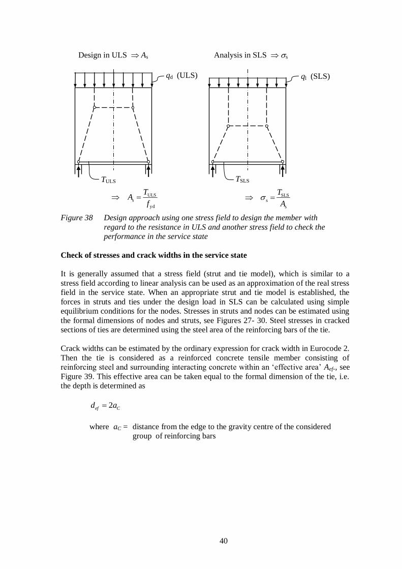
40

ql (SLS) qd (ULS)

TULS TSLS

yd

ULSs

f

TA

s

SLSs

A

T

Design in ULS As Analysis in SLS s

Figure 38 Design approach using one stress field to design the member with

regard to the resistance in ULS and another stress field to check the

performance in the service state

Check of stresses and crack widths in the service state

It is generally assumed that a stress field (strut and tie model), which is similar to a

stress field according to linear analysis can be used as an approximation of the real stress

field in the service state. When an appropriate strut and tie model is established, the

forces in struts and ties under the design load in SLS can be calculated using simple

equilibrium conditions for the nodes. Stresses in struts and nodes can be estimated using

the formal dimensions of nodes and struts, see Figures 27- 30. Steel stresses in cracked

sections of ties are determined using the steel area of the reinforcing bars of the tie.

Crack widths can be estimated by the ordinary expression for crack width in Eurocode 2.

Then the tie is considered as a reinforced concrete tensile member consisting of

reinforcing steel and surrounding interacting concrete within an ‘effective area’ Aef., see

Figure 39. This effective area can be taken equal to the formal dimension of the tie, i.e.

the depth is determined as

Cef ad 2

where aC = distance from the edge to the gravity centre of the considered

group of reinforcing bars

41

ql (SLS)

TSLS Aef Tie =

reinforced concrete Aef

def

Figure 39 The formal dimension of concentrated ties can be used as the

‘effective area’ in crack width calculations

3.3 Alternative strut and tie models

When theory of plasticity is adopted in the design of a statically indeterminate structure,

there is not one unique solution, but many alternative solutions are possible. Since stress

fields in discontinuity regions always are statically indeterminate, this is also true when

the strut and tie method is used in design. The ultimate load can be resisted in many

different ways, leading to alternative designs and strut and tie models. The stiffness

conditions and the stress field are significantly influenced by the amount and

arrangement of the reinforcement. This means that the designer to a considerable extent

can influence how the element carries the load and also the structural behaviour under

load increase. Figure 40 shows three alternative strut and tie models that all fulfil the

equilibrium conditions in the ultimate limit state.

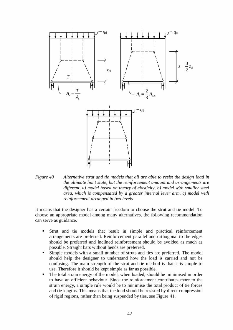
42

els,s3

2AA

qd

qd

s

sA

TA

qd

T

zel el

2

3zz

Figure 40 Alternative strut and tie models that all are able to resist the design load in

the ultimate limit state, but the reinforcement amount and arrangements are

different, a) model based on theory of elasticity, b) model with smaller steel

area, which is compensated by a greater internal lever arm, c) model with

reinforcement arranged in two levels

It means that the designer has a certain freedom to choose the strut and tie model. To

choose an appropriate model among many alternatives, the following recommendation

can serve as guidance.

Strut and tie models that result in simple and practical reinforcement

arrangements are preferred. Reinforcement parallel and orthogonal to the edges

should be preferred and inclined reinforcement should be avoided as much as

possible. Straight bars without bends are preferred.

Simple models with a small number of struts and ties are preferred. The model

should help the designer to understand how the load is carried and not be

confusing. The main strength of the strut and tie method is that it is simple to

use. Therefore it should be kept simple as far as possible.

The total strain energy of the model, when loaded, should be minimised in order

to have an efficient behaviour. Since the reinforcement contributes more to the

strain energy, a simple rule would be to minimise the total product of tie forces

and tie lengths. This means that the load should be resisted by direct compression

of rigid regions, rather than being suspended by ties, see Figure 41.

43

Strut and tie models that are similar to the linear elastic stress field are preferred

with regard to limited plastic deformation capacity of the real materials and the

need for an appropriate performance in the service state.

qd

z

qd

T

z

Figure 41 Alternative strut and tie models where the left should be preferred because of

a more efficient behaviour with less ties and smaller tie forces. The model to

the right also violates the principles of the load path method, which results in

a less good service performance and a need for more plastic redistribution.

This model also results in a less practical reinforcement arrangement,

adopted from Schlaich et al. (1987)

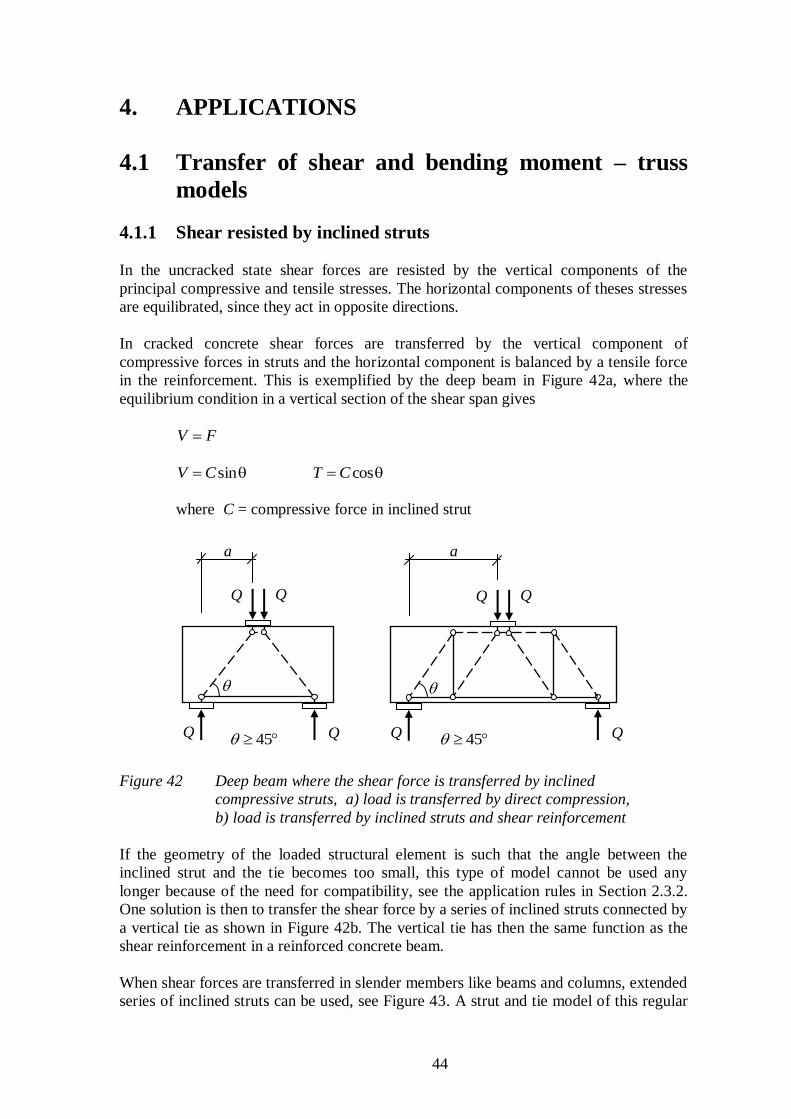
44

4. APPLICATIONS

4.1 Transfer of shear and bending moment – truss

models

4.1.1 Shear resisted by inclined struts

In the uncracked state shear forces are resisted by the vertical components of the

principal compressive and tensile stresses. The horizontal components of theses stresses

are equilibrated, since they act in opposite directions.

In cracked concrete shear forces are transferred by the vertical component of

compressive forces in struts and the horizontal component is balanced by a tensile force

in the reinforcement. This is exemplified by the deep beam in Figure 42a, where the

equilibrium condition in a vertical section of the shear span gives

FV

sinCV cosCT

where C = compressive force in inclined strut

Q Q

Q Q

45

a

Q Q

Q

Q 45

a

Figure 42 Deep beam where the shear force is transferred by inclined

compressive struts, a) load is transferred by direct compression,

b) load is transferred by inclined struts and shear reinforcement

If the geometry of the loaded structural element is such that the angle between the

inclined strut and the tie becomes too small, this type of model cannot be used any

longer because of the need for compatibility, see the application rules in Section 2.3.2.

One solution is then to transfer the shear force by a series of inclined struts connected by

a vertical tie as shown in Figure 42b. The vertical tie has then the same function as the

shear reinforcement in a reinforced concrete beam.

When shear forces are transferred in slender members like beams and columns, extended

series of inclined struts can be used, see Figure 43. A strut and tie model of this regular

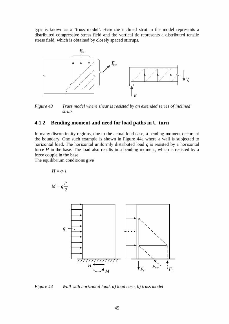
45

type is known as a ‘truss model’. Here the inclined strut in the model represents a

distributed compressive stress field and the vertical tie represents a distributed tensile

stress field, which is obtained by closely spaced stirrups.

Fsv

Fcw

R

Vd

Figure 43 Truss model where shear is resisted by an extended series of inclined

struts

4.1.2 Bending moment and need for load paths in U-turn

In many discontinuity regions, due to the actual load case, a bending moment occurs at

the boundary. One such example is shown in Figure 44a where a wall is subjected to

horizontal load. The horizontal uniformly distributed load q is resisted by a horizontal

force H in the base. The load also results in a bending moment, which is resisted by a

force couple in the base.

The equilibrium conditions give

lqH

2

2lqM

q

H

M Fs Fcw

Fc

Figure 44 Wall with horizontal load, a) load case, b) truss model

46

The load path between the load and the horizontal reaction H involves shear transfer.

This is obtained by inclined compressive struts that represent a distributed compressive

stress field. The truss model in Figure 44b is appropriate to simulate this stress field. The

strut line is represents the resultant of the stress field and should be located in the centre

of the assumed stress field where it meets the base. The horizontal reaction H

corresponds to the horizontal component of the inclined compressive force Fcw. For

vertical equilibrium it is obvious that the vertical component of this force Fcw influences

the forces in the force couple, see Section 4.1.3.

The truss model can be regarded as a combination of a load path in a zigzag pattern that

takes care of the shear force and a load path in U-turn that takes care of the moment, see

Figure 45. The load path in U-turn connects opposite forces at the boundary that are in

equilibrium and added to the main load path for load transfer. Load paths in U-turn

typically appear in problems where a bending moment is transferred at a boundary, see

Section 2.2. When the two load paths are combined, the forces in the U-turn will be

influenced by the other system, see Section 4.1.3.

H Fs

Fcw Fc

+ =

Figure 45 The truss model can be regarded as a combination of a load path in a

zigzag line and a load path in U-turn

4.1.3 Boundary between B- and D-regions

Where a discontinuity region (D-region) meets a continuity region (B-region) with shear

and bending, three contact forces can be defined, see Figure 46. These are an inclined

compressive force Fcw in the centre of the section (represents a distributed compressive

stress field), a concentrated compressive force Fc in the ‘compressive chord’ and a

concentrated tensile force Fs in the ‘tensile chord’.

The contact forces are related to the sectional forces by the following equilibrium

conditions. The shear force is resisted by the transverse component of the inclined

compressive force.

47

sin

VFcw

where = strut inclination

The horizontal component of the inclined compressive force corresponds to a normal

force N that must be balanced by the forces in the compressive and the tensile chords.

Hence, the force in one chord should resist the bending moment (force in force couple)

and half of the normal force N.

tan

cosV

FN cw

tan2

V

z

MFc (compressive force decreases due to inclined strut)

tan2

V

z

MFs (tensile force increases due to inclined strut)

R x

D-zone B-zone

Fc

Fcw

Fs

V(x)

M(x)

Figure 46 Contact forces where a D-region meets a B-region subjected to shear

and bending

4.1.4 Modelling of B-regions

The strut and tie method is a general tool, which can be used to model not only

discontinuity regions but also continuity regions. The response in bending is normally

analysed by the general sectional model, which is based on the assumption of linear

strain distribution (plane sections remaining plane). However, for the response in shear

of cracked reinforced members are nowadays normally analysed by strut and tie models.

They will then take the regular form that is known as ‘truss models’, see Figure 47.

48

Figure 47 Beam analysed by truss model

Truss models are helpful, since they help the designer to understand how equilibrium is

obtained in the cracked state by means of the reinforcement. For instance, the interaction

between the web and the flanges of beams with I- or T-sections and the need for

transverse reinforcement in the flanges can easily be understood by means of truss

models, see Figure 48.

Figure 48 Truss model for a reinforced concrete beam with I-section

4.2 Combination of vertical and horizontal loads on supports

Where simply supported structural members are placed on support bearings it is

common that the support should be designed for a combination of a vertical load Qd and

a horizontal load Hd as exemplified in Figure 49. In such case the two loads are replaced

49

by there inclined resultant. This can be assumed to be applied in the centre of the

interface between the bearing and the support.

Qd

Hd

N

Rd

Figure 49 Example of a support subjected to a combination of vertical and

horizontal loads, a) original load case, b) resulting load

In the support the stress field under the bearing is inclined until it reaches the horizontal

tie. This means that the node point in the strut and tie model is displaced from the

centreline of the bearing. The different cases with or without a horizontal load are shown

in Figure 50.

without Hd with Hd

y

Hd

Qd

Figure 50 Location of node point under the support bearing, a) load case without

horizontal load, b) load case with horizontal load

Consequently also the geometry of the node region is affected, which influences the

check of stresses in the node. The node in Figure 50b is a compression-tension node

with anchored ties in one direction. The compressive stresses should be checked in

sections perpendicular two the two inclined compressive stress fields, see Figure 51.

50

a2

a2/2

1

y

a1

Rd

c2

c1

a

as

as

Figure 51 Example of how a compression-tension node can be checked in a formal

way for a support with a combination of vertical and horizontal loads

The length of the critical sections can be determined as

cos1 aa

111

1

2 cos2sinsintan2

2

s

s aaaa

a

4.3 Problems in 3 D

4.3.1 Combination of 2-D models in perpendicular planes

Where a structural member is built up by plates that are arranged in different planes, as

for a beam with web and flanges, strut and tie models will be three-dimensional. In this

particular case, the problem can be analysed by a combination of 2-D models. One 2-D

model is developed for each plane. Some of the nodes will exist in both planes, see

Figure 52. These nodes, which connect the 2-D models, must be positioned correctly in

the respective models.

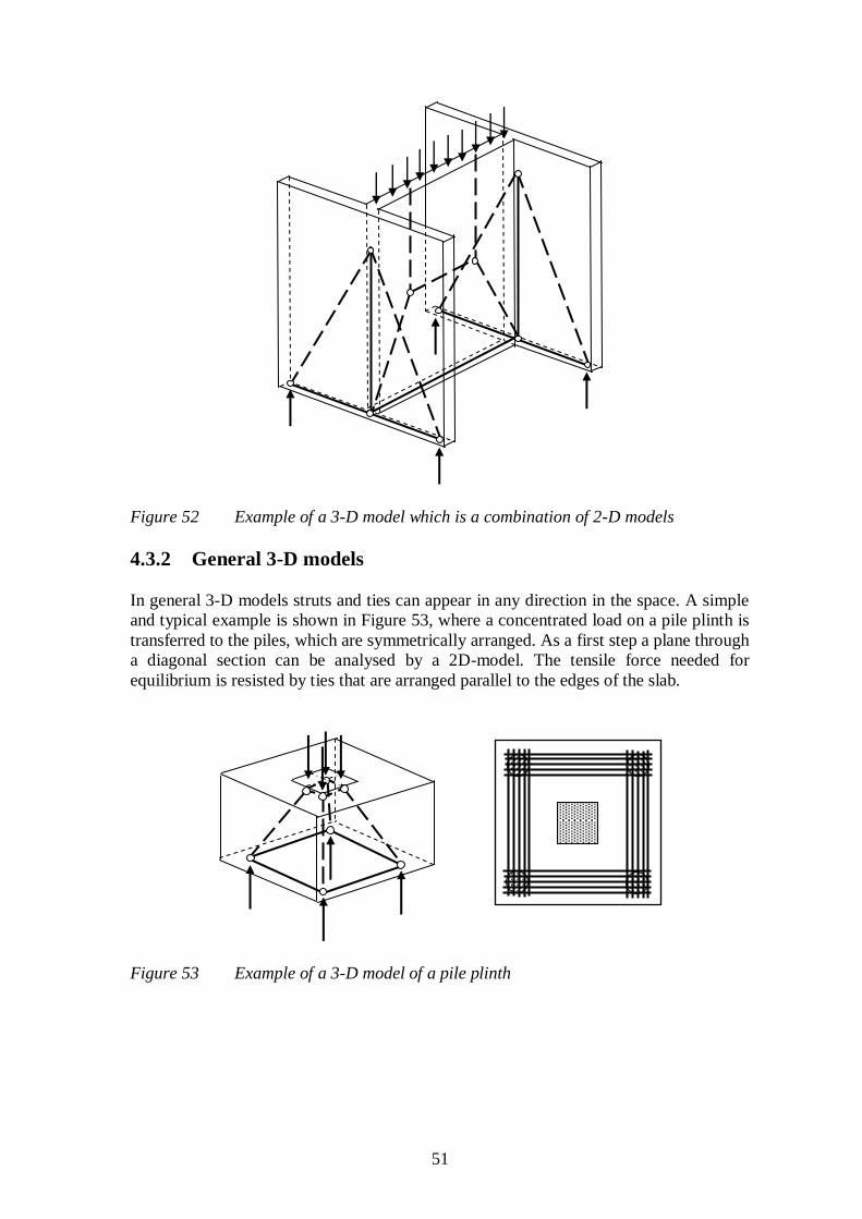
51

Figure 52 Example of a 3-D model which is a combination of 2-D models

4.3.2 General 3-D models

In general 3-D models struts and ties can appear in any direction in the space. A simple

and typical example is shown in Figure 53, where a concentrated load on a pile plinth is

transferred to the piles, which are symmetrically arranged. As a first step a plane through

a diagonal section can be analysed by a 2D-model. The tensile force needed for

equilibrium is resisted by ties that are arranged parallel to the edges of the slab.

Figure 53 Example of a 3-D model of a pile plinth

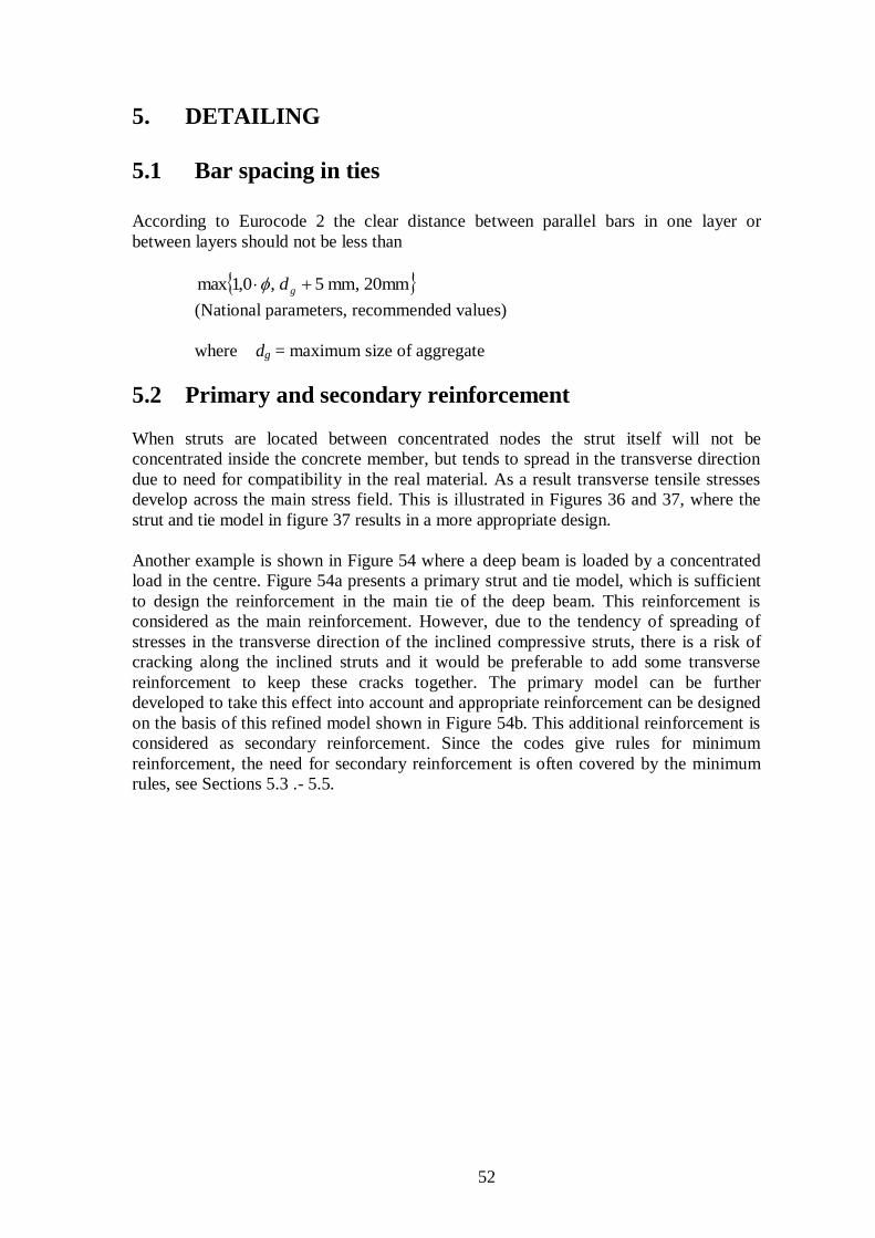
52

5. DETAILING

5.1 Bar spacing in ties

According to Eurocode 2 the clear distance between parallel bars in one layer or

between layers should not be less than

mm20,mm5,0,1max gd

(National parameters, recommended values)

where dg = maximum size of aggregate

5.2 Primary and secondary reinforcement

When struts are located between concentrated nodes the strut itself will not be

concentrated inside the concrete member, but tends to spread in the transverse direction

due to need for compatibility in the real material. As a result transverse tensile stresses

develop across the main stress field. This is illustrated in Figures 36 and 37, where the

strut and tie model in figure 37 results in a more appropriate design.

Another example is shown in Figure 54 where a deep beam is loaded by a concentrated

load in the centre. Figure 54a presents a primary strut and tie model, which is sufficient

to design the reinforcement in the main tie of the deep beam. This reinforcement is

considered as the main reinforcement. However, due to the tendency of spreading of

stresses in the transverse direction of the inclined compressive struts, there is a risk of

cracking along the inclined struts and it would be preferable to add some transverse

reinforcement to keep these cracks together. The primary model can be further

developed to take this effect into account and appropriate reinforcement can be designed

on the basis of this refined model shown in Figure 54b. This additional reinforcement is

considered as secondary reinforcement. Since the codes give rules for minimum

reinforcement, the need for secondary reinforcement is often covered by the minimum

rules, see Sections 5.3 .- 5.5.

53

a) b)

Figure 54 Deep beam with concentrated load, a) primary model, b) refined model

for design of secondary reinforcement

5.3 Deep beams

According to Eurocode 2 a beam is a structural member for which the span is greater

than or equal to 3 times the overall sectional depth. When the height is less than 3 times

the depth, the members should be considered as a deep beam.

The reinforcement corresponding to the main ties in the strut and tie model should be

fully anchored for equilibrium in the support nodes. If the length between the node and

the end of the deep beam is insufficient with regard to the needed design anchorage

length lbd, effective anchorage must be provided for instance by reinforcement bends, U-

hoops or anchorage devices.

Secondary reinforcement should normally be provided with an orthogonal mesh near

each face. The recommended minimum value of the reinforcement ratio is

001,0min

with an area not less than m/mm150 2

min, sA

Furthermore, the secondary reinforcement should have a maximum bar spacing

ts 2max not less than 300 mm

where t = thickness of the deep beam

54

5.4 Walls

According to Eurocode 2 the amount and detailing of reinforcement in reinforced

concrete walls may be determined from a strut and tie model. If vertical reinforcement is

taken into account in the analysis to resist vertical load, the area provided should,

according to Eurocode 2, fulfil minimum as well as maximum requirements.

The recommended limits of the area Asv of vertical structural reinforcement area are

csvc AAA 04,0002,0

The maximum amount refers to areas outside lap locations. In lap locations higher

amounts are permitted.

When the design is controlled by the minimum requirement above, half of this area

should be located at each face of the wall.

The maximum bar spacing of vertical structural reinforcement is given by

ts 3max not less than 400 mm

where t = thickness of the wall

Furthermore, horizontal reinforcement should be provided at each surface. The

recommended value of the area Ash of horizontal reinforcement is given by

svsh AA4

1 not less than csh AA 001,0

with a bar spacing not greater than 400max s mm

Transverse reinforcement in form of links should be provided

a) in regions where the total amount of vertical reinforcement exceeds 0,02Ac.

b) where the main reinforcement is placed nearest to the wall faces at least 4 links per

m2 wall area

5.5 Discontinuity regions

Discontinuity regions should, according to Eurocode 2, normally be designed with strut

and tie models. Reinforcement corresponding to the ties in the model should be fully

anchored with an anchorage length lbd.

55

REFERENCES

CEB-FIP (1993): Comite Euro-International du Beton: CEB-FIP Model Code 1990,

Thomas Telford, London 1993.

CEN (2004): European Committee for Standardisation: European Standard, EN

1992-1-1, Eurocode 2: Design of concrete structures – Part 1-1: General rules and

rules for buildings, Brussels, December 2004.

Nielsen (1984): Nielsen, M.P., Limit analysis and concrete plasticity, Prentice-Hall,

New Jersey, 1985.

Nilson (1987): Nilson, A. H.: High strength concrete - An overview of Cornell research,

Proceedings of the Symposium ‘Utilization of high strength concrete’, Stavanger,

Norway, June 1987, Tapir, Trondheim, pp. 27-38.

Richart et al. (1978): Richart, F. E., Brandtzaeg, A. and Brown, R. L.; A study of the

failure of concrete under combined compressive stresses, Bulletin No. 185, Engineering

experimental station, University of Illinois, 1978, 104 pp.

Schlaich et al. (1987): Schlaich, J., Schäfer, K. and Jennewein, M.: Toward a consistent

design of structural concrete, PCI Journal, Vol. 32, No. 2, May/June 1987, pp. 74-149.

Schlaich and Schäfer (1989): Schlaich, J. and Schäfer, K.: Theoretische Grundlagen –

Bemessen und Konstruiren mittels Stabwerkmodellen (Theoretical basis – analysis and

design with strut and tie models) and Anwendungen (Applications), Sections 3 and 4 in

Part E of Beton-Kalender 1989, Part 2, Ernst & Sohn, Berlin 1989, pp. 586-715 (In

German).

Schlaich and Schäfer (1991): Schlaich, J., Schäfer, K., Design and detailing of structural

concrete using strut-and-tie models, The Structural Engineer, Vol. 69, No, 6, March

1991.

Schäfer (1999a): Schäfer, K., Deep beams and discontinuity regions, Section 7.3 in

Structural Concrete, Vol. 3, fédération internationale de béton, Bulletin 3, Lausanne

1999.

Schäfer (1999b): Schäfer, K., Nodes, Section 4.4.4 in Structural Concrete, Vol. 2,

fédération internationale de béton, Bulletin 2, Lausanne 1999, pp. 257 – 275.

design and analysis of deep beams, plates and …...figure 1 stress field in the end of a...

Documents