descartes’ world of analytic geometry - kthcgjoh/preview/part5.pdf · 89.2 descartes, inventor of...
TRANSCRIPT
Part V
Descartes’ World ofAnalytic Geometry
356

This is page 357Printer: Opaque this
FIGURE 88.2. Descartes: The Principle which I have always observed in mystudies and which I believe has helped me the most to gain what knowledge Ihave, has been never to spend beyond a few hours daily in thoughts which occupythe imagination, and a few hours yearly in those which occupy the understanding,and to give all the rest of my time to the relaxation of the senses and the reposeof the mind...As for me, I have never presumed my mind to be in any way betterthan the minds of people in general. As for reason or good sense, I am inclinedto believe that it exists whole and complete in each of us, because it is the onlything that makes us men and distinguishes us from the lower animals.

This is page 358Printer: Opaque this

This is page 359Printer: Opaque this
89Analytic Geometry in R2
Philosophy is written in the great book (by which I mean the Uni-verse) which stands always open to our view, but it cannot be under-stood unless one first learns how to comprehend the language andinterpret the symbols in which it is written, and its symbols are tri-angles, circles, and other geometric figures, without which it is nothumanly possible to comprehend even one word of it; without theseone wanders in a dark labyrinth. (Galileo)
89.1 Introduction
We give a brief introduction to analytic geometry in two dimensions, thatis the linear algebra of the Euclidean plane. Our common school experiencehas given us an intuitive geometric idea of the Euclidean plane as an infi-nite flat surface without borders consisting of points, and we also have anintuitive geometric idea of geometric objects like straight lines, trianglesand circles in the plane. We brushed up our knowledge and intuition ingeometry somewhat in Chapter Pythagoras and Euclid. We also presentedthe idea of using a coordinate system in the Euclidean plane consistingof two perpendicular copies of Q, where each point in the plane has twocoordinates (a1, a2) and we view Q2 as the set of ordered pairs of rationalnumbers. With only the rational numbers Q at our disposal, we quickly runinto trouble because we cannot compute distances between points in Q2.For example, the distance between the points (0, 0) and (1, 1), the length ofthe diagonal of a unit square, is equal to
√2, which is not a rational num-
360 89. Analytic Geometry in R2
ber. The troubles are resolved by using real numbers, that is by extendingQ2 to R2.In this chapter, we present basic aspects of analytic geometry in the
Euclidean plane using a coordinate system identified with R2, followingthe fundamental idea of Descartes to describe geometry in terms of num-bers. Below, we extend to analytic geometry in three-dimensional Euclideanspace identified with R3 and we finally generalize to analytic geometry inRn, where the dimension n can be any natural number. Considering Rn
with n ≥ 4 leads to linear algebra with a wealth of applications outsideEuclidean geometry, which we will meet below. The concepts and toolswe develop in this chapter focussed on Euclidean geometry in R2 will beof fundamental use in the generalizations to geometry in R3 and Rn andlinear algebra.The tools of the geometry of Euclid is the ruler and the compasses, while
the tool of analytic geometry is a calculator for computing with numbers.Thus we may say that Euclid represents a form of analog technique, whileanalytic geometry is a digital technique based on numbers. Today, the useof digital techniques is exploding in communication and music and all sortsof virtual reality.
89.2 Descartes, Inventor of Analytic Geometry
The foundation of modern science was laid by Rene Descartes (1596-1650)in Discours de la method pour bien conduire sa raison et chercher la veritedans les sciences from 1637. The Method contained as an appendix La Ge-ometrie with the first treatment of Analytic Geometry. Descartes believedthat only mathematics may be certain, so all must be based on mathemat-ics, the foundation of the Cartesian view of the World.In 1649 Queen Christina of Sweden persuaded Descartes to go to Stock-
holm to teach her mathematics. However the Queen wanted to draw tan-gents at 5 a.m. and Descartes broke the habit of his lifetime of getting upat 11 o’clock, c.f. Fig. 190.1. After only a few months in the cold North-ern climate, walking to the palace at 5 o’clock every morning, he died ofpneumonia.
89.3 Descartes: Dualism of Body and Soul
Descartes set the standard for studies of Body and Soul for a long time withhis De homine completed in 1633, where Descartes proposed a mechanismfor automatic reaction in response to external events through nerve fibrils,see Fig. 190.2. In Descartes’ conception, the rational Soul, an entity distinctfrom the Body and making contact with the body at the pineal gland,

89.4 The Euclidean Plane R2 361
might or might not become aware of the differential outflow of animalspirits brought about though the nerve fibrils. When such awareness didoccur, the result was conscious sensation – Body affecting Soul. In turn,in voluntary action, the Soul might itself initiate a differential outflow ofanimal spirits. Soul, in other words, could also affect Body.In 1649 Descartes completed Les passions de l’ame, with an account of
causal Soul/Body interaction and the conjecture of the localization of theSoul’s contact with the Body to the pineal gland. Descartes chose the pinealgland because it appeared to him to be the only organ in the brain thatwas not bilaterally duplicated and because he believed, erroneously, thatit was uniquely human; Descartes considered animals as purely physicalautomata devoid of mental states.
FIGURE 89.1. Automatic reaction in response to external stimulation fromDescartes De homine 1662.
89.4 The Euclidean Plane R2
We choose a coordinate system for the Euclidean plane consisting of twostraight lines intersecting at a 90 angle at a point referred to as the origin.One of the lines is called the x1-axis and the other the x2-axis, and eachline is a copy of the real line R. The coordinates of a given point a in theplane is the ordered pair of real numbers (a1, a2), where a1 corresponds tothe intersection of the x1-axis with a line through a parallel to the x2-axis,and a2 corresponds to the intersection of the x2-axis with a line througha parallel to the x1-axis, see Fig. 190.3. The coordinates of the origin are(0, 0).

362 89. Analytic Geometry in R2
In this way, we identify each point a in the plane with its coordinates(a1, a2), and we may thus represent the Euclidean plane as R2, where R2
is the set of ordered pairs (a1, a2) of real numbers a1 and a2. That is
R2 = (a1, a2) : a1, a2 ∈ R.
We have already used R2 as a coordinate system above when plotting afunction f : R → R, where pairs of real numbers (x, f(x)) are representedas geometrical points in a Euclidean plane on a book-page.
/PSfrag wherepop(x1)[[0(Bl)1 0]](x2)[[1(Bl)1 0]](a1)[[2(Bl)1 0]](a2)[[3(Bl)1 0]]((a1,a2))[[4(Bl)1 0]]5 0 1/Begin PSfraguserdict /PSfragpopputifelse
x2
a1
a2(a1,a2)
x1
/End PSfrag /Hide PSfragPSfrag replacements/Unhide PSfrag– x1 0/Place PSfrag– x2 1/Place PSfrag– a1 2/Place PSfrag– a2 3/Place PSfrag– (a1, a2)˝ 4/Place PSfrag
FIGURE 89.2. Coordinate system for R2
To be more precise, we can identify the Euclidean plane with R2, oncewe have chosen the (i) origin, and the (ii) direction (iii) scaling of the co-ordinate axes. There are many possible coordinate systems with differentorigins and orientations/scalings of the coordinate axes, and the coordi-nates of a geometrical point depend on the choice of coordinate system.The need to change coordinates from one system to another thus quicklyarises, and will be an important topic below.Often, we orient the axes so that the x1-axis is horizontal and increas-
ing to the right, and the x2-axis is obtained rotating the x1 axis by 90,or a quarter of a complete revolution counter-clockwise, see Fig. 190.3 orFig. 190.4 displaying MATLAB’s view of a coordinate system. The posi-tive direction of each coordinate axis may be indicated by an arrow in thedirection of increasing coordinates.However, this is just one possibility. For example, to describe the position
of points on a computer screen or a window on such a screen, it is notuncommon to use coordinate systems with the origin at the upper leftcorner and counting the a2 coordinate positive down, negative up.

89.5 Surveyors and Navigators 363
/PSfrag wherepop(x1)[[0(Bl)1 0]](x2)[[1(Bl)1 0]](“(.5,.2“))[[2(Bl)1 0]]3 0 1/Begin PSfraguserdict /PSfragpopputifelse−0.4 −0.2 0 0.2 0.4 0.6 0.8 1 1.2 1.4
−0.8
−0.6
−0.4
−0.2
0
0.2
0.4
0.6
0.8
x1
x2
(.5,.2)
/End PSfrag /Hide PSfragPSfrag replacements/Unhide PSfrag– x1 0/Place PSfrag– x1 1/Place PSfrag– (.5, .2)˝ 2/Place PSfrag
FIGURE 89.3. Matlabs way of visualizing a coordinate system for a plane.
89.5 Surveyors and Navigators
Recall our friends the Surveyor in charge of dividing land into properties,and the Navigator in charge of steering a ship. In both cases we assume thatthe distances involved are sufficiently small to make the curvature of theEarth negligible, so that we may view the world as R2. Basic problems facedby a Surveyor are (s1) to locate points in Nature with given coordinateson a map and (s2) to compute the area of a property knowing its corners.Basic problems of a Navigator are (n1) to find the coordinates on a map ofhis present position in Nature and (n2) to determine the present directionto follow to reach a point of destiny.We know from Chapter 2 that problem (n1) may be solved using a GPS
navigator, which gives the coordinates (a1, a2) of the current position ofthe GPS-navigator at a press of a button. Also problem (s1) may be solvedusing a GPS-navigator iteratively in an ‘inverse” manner: press the buttonand check where we are and move appropriately if our coordinates are notthe desired ones. In practice, the precision of the GPS-system determinesits usefulness and increasing the precision normally opens a new area ofapplication. The standard GPS with a precision of 10 meters may be OKfor a navigator, but not for a surveyor, who would like to get down tometers or centimeters depending on the scale of the property. Scientistsmeasuring continental drift or beginning landslides, use an advanced formof GPS with a precision of millimeters.Having solved the problems (s1) and (n1) of finding the coordinates of a
given point in Nature or vice versa, there are many related problems of type(s2) or (n2) that can be solved using mathematics, such as computing thearea of pieces of land with given coordinates or computing the direction of apiece of a straight line with given start and end points. These are examples

364 89. Analytic Geometry in R2
of basic problems of geometry, which we now approach to solve using toolsof analytic geometry or linear algebra.
89.6 A First Glimpse of Vectors
Before entering into analytic geometry, we observe that R2, viewed as theset of ordered pairs of real numbers, can be used for other purposes thanrepresenting positions of geometric points. For example to describe thecurrent weather, we could agree to write (27, 1013) to describe that thetemperature is 27 C and the air pressure 1013 millibar. We then describe acertain weather situation as an ordered pair of numbers, such as (27, 1013).Of course the order of the two numbers is critical for the interpretation. Aweather situation described by the pair (1013, 27) with temperature 1013and pressure 27, is certainly very different from that described by (27, 1013)with temperature 27 and pressure 1013.Having liberated ourselves from the idea that a pair of numbers must
represent the coordinates of a point in a Euclidean plane, there are end-less possibilities of forming pairs of numbers with the numbers representingdifferent things. Each new interpretation may be viewed as a new interpre-tation of R2.In another example related to the weather, we could agree to write
(8, NNE) to describe that the current wind is 8 m/s and headed North-North-East (and coming from South-South-East. Now, NNE is not a realnumber, so in order to couple to R2, we replace NNE by the correspondingangle, that is by 22.5 counted positive clockwise starting from the Northdirection. We could thus indicate a particular wind speed and directionby the ordered pair (8, 22.5). You are no doubt familiar with the weatherman’s way of visualizing such a wind on the weather map using an arrow.The wind arrow could also be described in terms of another pair of
parameters, namely by how much it extends to the East and to the Northrespectively, that is by the pair (8 sin(22.5), 8 cos(22.5)) ≈ (3.06, 7.39).We could say that 3.06 is the “amount of East”, and 7.39 is the “amountof North” of the wind velocity, while we may say that the wind speed is 8,where we think of the speed as the “absolute value” of the wind velocity(3.06, 7.39). We thus think of the wind velocity as having both a direction,and an “absolute value” or “length”. In this case, we view an ordered pair(a1, a2) as a vector, rather than as a point, and we can then represent thevector by an arrow.We will soon see that ordered pairs viewed as vectors may be scaled
through multiplication by a real number and two vectors may also be added.Addition of velocity vectors can be experienced on a bike where the wind
velocity and our own velocity relative to the ground add together to formthe total velocity relative to the surrounding atmosphere, which is reflected

89.7 Ordered Pairs as Points or Vectors/Arrows 365
in the air resistance we feel. To compute the total flight time across theAtlantic, the airplane pilot adds the velocity vector of the airplane versusthe atmosphere and the velocity of the jet-stream together to obtain thevelocity of the airplane vs the ground. We will return below to applicationsof analytic geometry to mechanics, including these examples.
89.7 Ordered Pairs as Points or Vectors/Arrows
We have seen that we may interpret an ordered pair of real numbers (a1, a2)as a point a in R2 with coordinates a1 and a2. We may write a = (a1, a2)for short, and say that a1 is the first coordinate of the point a and a2 thesecond coordinate of a.We shall also interpret an ordered pair (a1, a2) ∈ R2 in a alternative
way, namely as an arrow with tail at the origin and the head at the pointa = (a1, a2), see Fig. 190.5. With the arrow interpretation of (a1, a2), werefer to (a1, a2) as a vector. Again, we agree to write a = (a1, a2), and wesay that a1 and a2 are the components of the arrow/vector a = (a1, a2).We say that a1 is the first component, occurring in the first place and a2the second component occurring in the second place.
/PSfrag wherepop(x1)[[0(Bl)1 0]](x2)[[1(Bl)1 0]](a1)[[2(Bl)1 0]](a2)[[3(Bl)1 0]](a)[[4(Bl)1 0]]((a1,a2))[[5(Bl)1 0]]6 0 1/Begin PSfraguserdict /PSfragpopputifelse
a
a1
a2
x2
x1
(a1,a2)
/End PSfrag /Hide PSfragPSfrag replacements/Unhide PSfrag– x1 0/Place PSfrag– x2 1/Place PSfrag– a1 2/Place PSfrag– a2 3/Place PSfrag– a 4/Place PSfrag– (a1, a2)˝ 5/Place PSfrag
FIGURE 89.4. A vector with tail at the origin and the head at the pointa = (a1, a2)
We thus may interpret an ordered pair (a1, a2) in R2 in two ways: asa point with coordinates (a1, a2), or as an arrow/vector with components(a1, a2) starting at the origin and ending at the point (a1, a2). Evidently,there is a very strong connection between the point and arrow interpreta-tions, since the head of the arrow is located at the point (and assuming thatthe arrow tail is at the origin). In applications, positions will be connectedto the point interpretation and velocities and forces will be connected to
366 89. Analytic Geometry in R2
the arrow/vector interpretation. We will below generalize the arrow/vectorinterpretation to include arrows with tails also at other points than theorigin. The context will indicate which interpretation is most appropriatefor a given situation. Often the interpretation of a = (a1, a2) as a pointor as an arrow, changes without notice. So we have to be flexible and usewhatever interpretation is most convenient or appropriate. We will needeven more fantasy when we go into applications to mechanics below.Sometimes vectors like a = (a1, a2) are marked by boldface or an arrow,
like a or a or a, or double script or some other notation. We prefer notto use this more elaborate notation, which makes the writing simpler, butrequires fantasy from the user to make the proper interpretation of forexample the letter a as a scalar number or vector a = (a1, a2) or somethingelse.
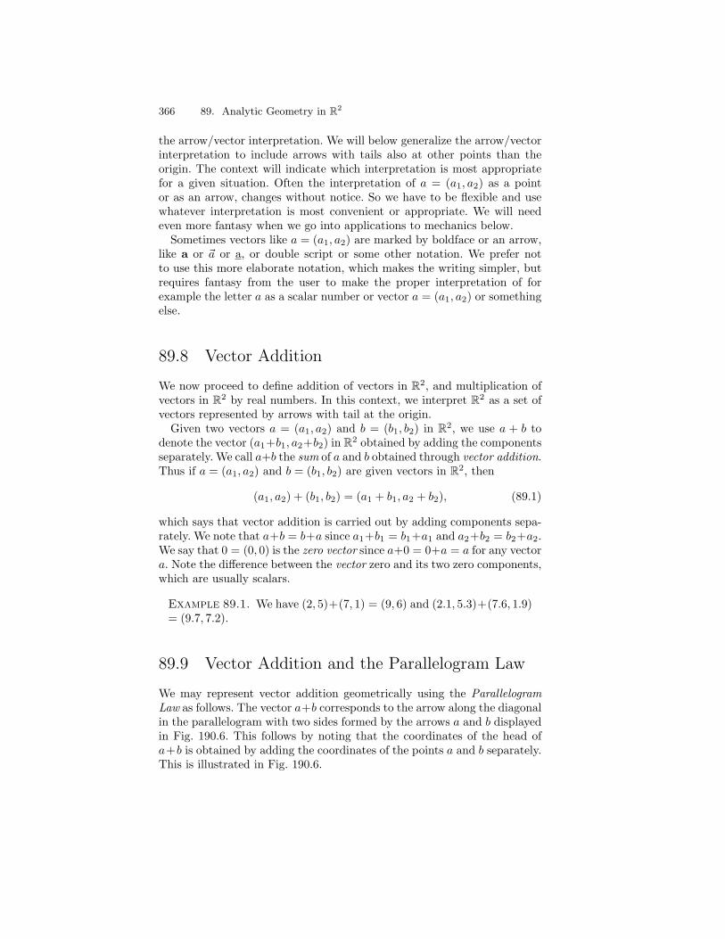
89.8 Vector Addition
We now proceed to define addition of vectors in R2, and multiplication ofvectors in R2 by real numbers. In this context, we interpret R2 as a set ofvectors represented by arrows with tail at the origin.Given two vectors a = (a1, a2) and b = (b1, b2) in R2, we use a + b to
denote the vector (a1+b1, a2+b2) in R2 obtained by adding the componentsseparately. We call a+b the sum of a and b obtained through vector addition.Thus if a = (a1, a2) and b = (b1, b2) are given vectors in R2, then
(a1, a2) + (b1, b2) = (a1 + b1, a2 + b2), (89.1)
which says that vector addition is carried out by adding components sepa-rately. We note that a+b = b+a since a1+b1 = b1+a1 and a2+b2 = b2+a2.We say that 0 = (0, 0) is the zero vector since a+0 = 0+a = a for any vectora. Note the difference between the vector zero and its two zero components,which are usually scalars.
Example 89.1. We have (2, 5)+(7, 1) = (9, 6) and (2.1, 5.3)+(7.6, 1.9)= (9.7, 7.2).
89.9 Vector Addition and the Parallelogram Law
We may represent vector addition geometrically using the ParallelogramLaw as follows. The vector a+b corresponds to the arrow along the diagonalin the parallelogram with two sides formed by the arrows a and b displayedin Fig. 190.6. This follows by noting that the coordinates of the head ofa+b is obtained by adding the coordinates of the points a and b separately.This is illustrated in Fig. 190.6.
89.10 Multiplication of a Vector by a Real Number 367
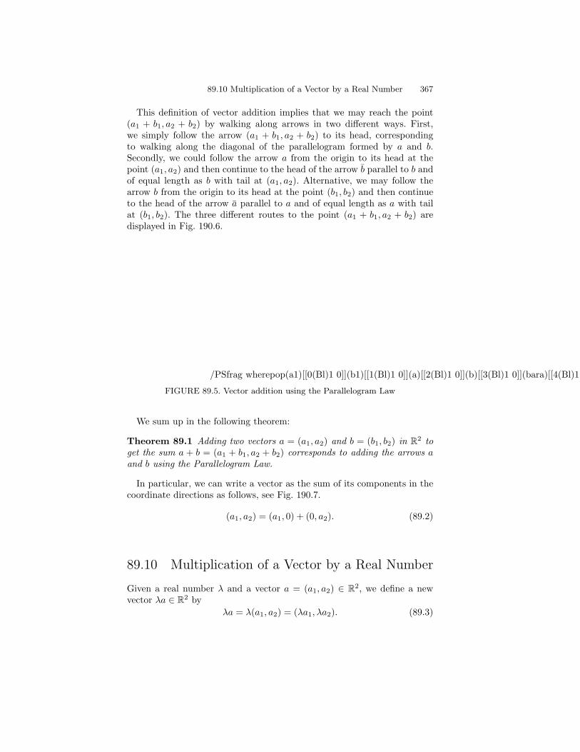
This definition of vector addition implies that we may reach the point(a1 + b1, a2 + b2) by walking along arrows in two different ways. First,we simply follow the arrow (a1 + b1, a2 + b2) to its head, correspondingto walking along the diagonal of the parallelogram formed by a and b.Secondly, we could follow the arrow a from the origin to its head at thepoint (a1, a2) and then continue to the head of the arrow b parallel to b andof equal length as b with tail at (a1, a2). Alternative, we may follow thearrow b from the origin to its head at the point (b1, b2) and then continueto the head of the arrow a parallel to a and of equal length as a with tailat (b1, b2). The three different routes to the point (a1 + b1, a2 + b2) aredisplayed in Fig. 190.6.
/PSfrag wherepop(a1)[[0(Bl)1 0]](b1)[[1(Bl)1 0]](a)[[2(Bl)1 0]](b)[[3(Bl)1 0]](bara)[[4(Bl)1 0]](barb)[[5(Bl)1 0]](a+b)[[6(Bl)1 0]]7 0 1/Begin PSfraguserdict /PSfragpopputifelse
a1 b1
bara
barb
b
a
a+b
/End PSfrag /Hide PSfragPSfrag replacements/Unhide PSfrag– a1 0/Place PSfrag– b1 1/Place PSfrag– a 2/Place PSfrag– b 3/Place PSfrag– a 4/Place PSfrag– b 5/Place PSfrag– a+b˝ 6/Place PSfrag
FIGURE 89.5. Vector addition using the Parallelogram Law
We sum up in the following theorem:
Theorem 89.1 Adding two vectors a = (a1, a2) and b = (b1, b2) in R2 toget the sum a + b = (a1 + b1, a2 + b2) corresponds to adding the arrows aand b using the Parallelogram Law.
In particular, we can write a vector as the sum of its components in thecoordinate directions as follows, see Fig. 190.7.
(a1, a2) = (a1, 0) + (0, a2). (89.2)
89.10 Multiplication of a Vector by a Real Number
Given a real number λ and a vector a = (a1, a2) ∈ R2, we define a newvector λa ∈ R2 by
λa = λ(a1, a2) = (λa1, λa2). (89.3)
368 89. Analytic Geometry in R2
/PSfrag wherepop(a)[[0(Bl)1 0]]((a1,0))[[1(Bl)1 0]]((0,a2))[[2(Bl)1 0]]3 0 1/Begin PSfraguserdict /PSfragpopputifelse
a
(a1,0)
(0,a2)
/End PSfrag /Hide PSfragPSfrag replacements/Unhide PSfrag– a 0/Place PSfrag– (a1, 0)˝ 1/Place PSfrag– (0, a2)˝ 2/Place PSfrag
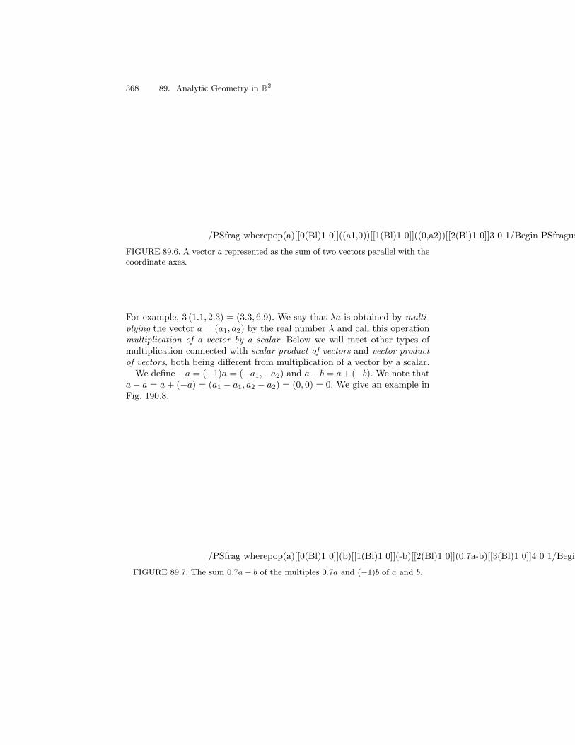
FIGURE 89.6. A vector a represented as the sum of two vectors parallel with thecoordinate axes.
For example, 3 (1.1, 2.3) = (3.3, 6.9). We say that λa is obtained by multi-plying the vector a = (a1, a2) by the real number λ and call this operationmultiplication of a vector by a scalar. Below we will meet other types ofmultiplication connected with scalar product of vectors and vector productof vectors, both being different from multiplication of a vector by a scalar.We define −a = (−1)a = (−a1,−a2) and a− b = a+(−b). We note that
a− a = a+ (−a) = (a1 − a1, a2 − a2) = (0, 0) = 0. We give an example inFig. 190.8.
/PSfrag wherepop(a)[[0(Bl)1 0]](b)[[1(Bl)1 0]](-b)[[2(Bl)1 0]](0.7a-b)[[3(Bl)1 0]]4 0 1/Begin PSfraguserdict /PSfragpopputifelse
−b
a
0.7a−b
b
/End PSfrag /Hide PSfragPSfrag replacements/Unhide PSfrag– a 0/Place PSfrag– b 1/Place PSfrag– −b2/Place PSfrag– 0.7a− b˝ 3/Place PSfrag
FIGURE 89.7. The sum 0.7a− b of the multiples 0.7a and (−1)b of a and b.
89.11 The Norm of a Vector 369
89.11 The Norm of a Vector
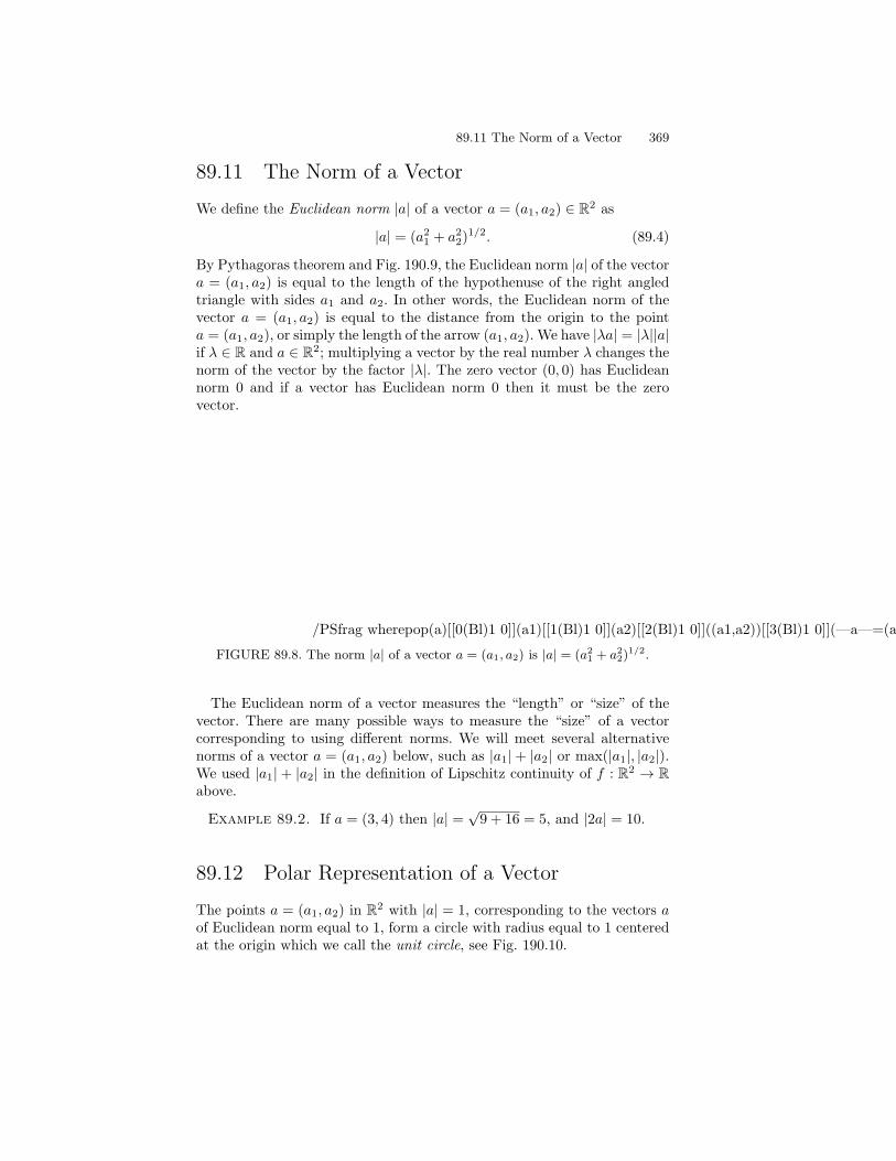
We define the Euclidean norm |a| of a vector a = (a1, a2) ∈ R2 as
|a| = (a21 + a22)1/2. (89.4)
By Pythagoras theorem and Fig. 190.9, the Euclidean norm |a| of the vectora = (a1, a2) is equal to the length of the hypothenuse of the right angledtriangle with sides a1 and a2. In other words, the Euclidean norm of thevector a = (a1, a2) is equal to the distance from the origin to the pointa = (a1, a2), or simply the length of the arrow (a1, a2). We have |λa| = |λ||a|if λ ∈ R and a ∈ R2; multiplying a vector by the real number λ changes thenorm of the vector by the factor |λ|. The zero vector (0, 0) has Euclideannorm 0 and if a vector has Euclidean norm 0 then it must be the zerovector.
/PSfrag wherepop(a)[[0(Bl)1 0]](a1)[[1(Bl)1 0]](a2)[[2(Bl)1 0]]((a1,a2))[[3(Bl)1 0]](—a—=(a12+a22)1/2)[[4(Bl)1 0]]5 0 1/Begin PSfraguserdict /PSfragpopputifelse
a
a1
(a1,a2)
|a|=(a12+a22)1/2
a2
/End PSfrag /Hide PSfragPSfrag replacements/Unhide PSfrag– a 0/Place PSfrag– a1 1/Place PSfrag– a2 2/Place PSfrag– (a1, a2)˝ 3/Place PSfrag– |a| = (a21 + a2
2)1/2˝ 4/Place PSfrag
FIGURE 89.8. The norm |a| of a vector a = (a1, a2) is |a| = (a21 + a2
2)1/2.
The Euclidean norm of a vector measures the “length” or “size” of thevector. There are many possible ways to measure the “size” of a vectorcorresponding to using different norms. We will meet several alternativenorms of a vector a = (a1, a2) below, such as |a1|+ |a2| or max(|a1|, |a2|).We used |a1|+ |a2| in the definition of Lipschitz continuity of f : R2 → Rabove.
Example 89.2. If a = (3, 4) then |a| =√9 + 16 = 5, and |2a| = 10.
89.12 Polar Representation of a Vector
The points a = (a1, a2) in R2 with |a| = 1, corresponding to the vectors aof Euclidean norm equal to 1, form a circle with radius equal to 1 centeredat the origin which we call the unit circle, see Fig. 190.10.

370 89. Analytic Geometry in R2
Each point a on the unit circle can be written a = (cos(θ), sin(θ)) forsome angle θ, which we refer to as the angle of direction or direction of thevector a. This follows from the definition of cos(θ) and sin(θ) in ChapterPythagoras and Euclid, see Fig. 190.10
/PSfrag wherepop(1)[[0(Bl)1 0]](a)[[1(Bl)1 0]](x1)[[2(Bl)1 0]](x2)[[3(Bl)1 0]](a1)[[4(Bl)1 0]](a2)[[5(Bl)1 0]](theta)[[6(Bl)1 0]](—a—=1)[[7(Bl)1 0]](a1=cos(theta))[[8(Bl)1 0]](a2=sin(theta))[[9(Bl)1 0]]10 0 1/Begin PSfraguserdict /PSfragpopputifelse
1
1
a1
a1=cos(theta)
a2=sin(theta)
theta
x2
a2|a|=1
a
x1
/End PSfrag /Hide PSfragPSfrag replacements/Unhide PSfrag– 1 0/Place PSfrag– a 1/Place PSfrag– x1 2/Place PSfrag– x2 3/Place PSfrag– a1 4/Place PSfrag– a2 5/Place PSfrag– θ 6/Place PSfrag– |a| = 1˝ 7/Place PSfrag– a1 = cos(θ)˝ 8/Place PSfrag– a2 = sin(θ)˝ 9/Place PSfrag
FIGURE 89.9. Vectors of length one are given by (cos(θ), sin(θ))
Any vector a = (a1, a2) = (0, 0) can be expressed as
a = |a|a = r(cos(θ), sin(θ)), (89.5)
where r = |a| is the norm of a, a = (a1/|a|, a2/|a|) is a vector of lengthone, and θ is the angle of direction of a, see Fig. 190.11. We call (190.5)the polar representation of a. We call θ the direction of a and r the lengthof a, see Fig. 190.11.
/PSfrag wherepop(r)[[0(Bl)1 0]](a)[[1(Bl)1 0]](x1)[[2(Bl)1 0]](x2)[[3(Bl)1 0]](a1)[[4(Bl)1 0]](a2)[[5(Bl)1 0]](theta)[[6(Bl)1 0]](—a—=r)[[7(Bl)1 0]](a1=rcos(theta))[[8(Bl)1 0]](a2=rsin(theta))[[9(Bl)1 0]]10 0 1/Begin PSfraguserdict /PSfragpopputifelse
r
ra1
theta
x1
x2
a2=rsin(theta)
a1=rcos(theta)a2
a
|a|=r
/End PSfrag /Hide PSfragPSfrag replacements/Unhide PSfrag– r 0/Place PSfrag– a 1/Place PSfrag– x1 2/Place PSfrag– x2 3/Place PSfrag– a1 4/Place PSfrag– a2 5/Place PSfrag– θ 6/Place PSfrag– |a| = r˝ 7/Place PSfrag– a1 = r cos(θ)˝ 8/Place PSfrag– a2 = r sin(θ)˝ 9/Place PSfrag
FIGURE 89.10. Vectors of length r are given bya = r(cos(θ), sin(θ)) = (r cos(θ), r sin(θ)) where r = |a|.

89.13 Standard Basis Vectors 371
We see that if b = λa, where λ > 0 and a = 0, then b has the samedirection as a. If λ < 0 then b has the opposite direction. In both cases,the norms change with the factor |λ|; we have |b| = |λ||a|.If b = λa, where λ = 0 and a = 0, then we say that the vector b is parallel
to a. Two parallel vectors have the same or opposite directions.
Example 89.3. We have
(1, 1) =√2(cos(45), sin(45)) and (−1, 1) =
√2(cos(135), sin(135)).
89.13 Standard Basis Vectors
We refer to the vectors e1 = (1, 0) and e2 = (0, 1) as the standard basisvectors in R2. A vector a = (a1, a2) can be expressed in term of the basisvectors e1 and e2 as
a = a1e1 + a2e2,
since
a1e1 + a2e2 = a1(1, 0) + a2(0, 1) = (a1, 0) + (0, a2) = (a1, a2) = a.
/PSfrag wherepop(a)[[0(Bl)1 0]](e1)[[1(Bl)1 0]](e2)[[2(Bl)1 0]]((a1,a2))[[3(Bl)1 0]](a=a1e1+a2e2)[[4(Bl)1 0]]5 0 1/Begin PSfraguserdict /PSfragpopputifelse
(a1,a2)
e1
e2
aa=a1e1+a2e2
/End PSfrag /Hide PSfragPSfrag replacements/Unhide PSfrag– a 0/Place PSfrag– e1 1/Place PSfrag– e2 2/Place PSfrag– (a1, a2)˝ 3/Place PSfrag– a = a1e1 + a2e2˝ 4/Place PSfrag
FIGURE 89.11. The standard basis vectors e1 and e2 and a linear combinationa = (a1, a2) = a1e1 + a2e2 of e1 and e2.
We say that a1e1 + a2e2 is a linear combination of e1 and e2 with coeffi-cients a1 and a2. Any vector a = (a1, a2) in R2 can thus be expressed as alinear combination of the basis vectors e1 and e2 with the coordinates a1and a2 as coefficients, see Fig. 190.12.
Example 89.4. We have (3, 7) = 3 (1, 0) + 7 (0, 1) = 3e1 + 7e2.
372 89. Analytic Geometry in R2
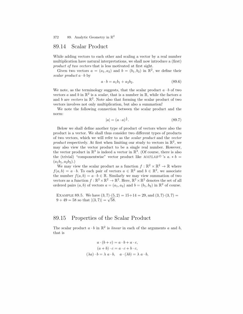
89.14 Scalar Product
While adding vectors to each other and scaling a vector by a real numbermultiplication have natural interpretations, we shall now introduce a (first)product of two vectors that is less motivated at first sight.Given two vectors a = (a1, a2) and b = (b1, b2) in R2, we define their
scalar product a · b by
a · b = a1b1 + a2b2. (89.6)
We note, as the terminology suggests, that the scalar product a · b of twovectors a and b in R2 is a scalar, that is a number in R, while the factors aand b are vectors in R2. Note also that forming the scalar product of twovectors involves not only multiplication, but also a summation!We note the following connection between the scalar product and the
norm:
|a| = (a · a) 12 . (89.7)
Below we shall define another type of product of vectors where also theproduct is a vector. We shall thus consider two different types of productsof two vectors, which we will refer to as the scalar product and the vectorproduct respectively. At first when limiting our study to vectors in R2, wemay also view the vector product to be a single real number. However,the vector product in R3 is indeed a vector in R3. (Of course, there is alsothe (trivial) “componentwise” vector product like MATLAB c⃝ ’s a. ∗ b =(a1b1, a2b2).)We may view the scalar product as a function f : R2 × R2 → R where
f(a, b) = a · b. To each pair of vectors a ∈ R2 and b ∈ R2, we associatethe number f(a, b) = a · b ∈ R. Similarly we may view summation of twovectors as a function f : R2×R2 → R2. Here, R2×R2 denotes the set of allordered pairs (a, b) of vectors a = (a1, a2) and b = (b1, b2) in R2 of course.
Example 89.5. We have (3, 7)·(5, 2) = 15+14 = 29, and (3, 7)·(3, 7) =9 + 49 = 58 so that |(3, 7)| =
√58.
89.15 Properties of the Scalar Product
The scalar product a · b in R2 is linear in each of the arguments a and b,that is
a · (b+ c) = a · b+ a · c,(a+ b) · c = a · c+ b · c,
(λa) · b = λ a · b, a · (λb) = λ a · b,

89.16 Geometric Interpretation of the Scalar Product 373
for all a, b ∈ R2 and λ ∈ R. This follows directly from the definition (190.6).For example, we have
a · (b+ c) = a1(b1 + c1) + a2(b2 + c2)
= a1b1 + a2b2 + a1c1 + a2c2 = a · b+ a · c.
Using the notation f(a, b) = a · b, the linearity properties may be writtenas
f(a, b+ c) = f(a, b) + f(a, c), f(a+ b, c) = f(a, c) + f(b, c),
f(λa, b) = λf(a, b) f(a, λb) = λf(a, b).
We also say that the scalar product a · b = f(a, b) is a bilinear form onR2 ×R2, that is a function from R2 ×R2 to R, since a · b = f(a, b) is a realnumber for each pair of vectors a and b in R2 and a · b = f(a, b) is linearboth in the variable (or argument) a and the variable b. Furthermore, thescalar product a · b = f(a, b) is symmetric in the sense that
a · b = b · a or f(a, b) = f(b, a),
and positive definite, that is
a · a = |a|2 > 0 for a = 0 = (0, 0).
We may summarize by saying that the scalar product a · b = f(a, b) is abilinear symmetric positive definite form on R2 × R2.We notice that for the basis vectors e1 = (1, 0) and e2 = (0, 1), we have
e1 · e2 = 0, e1 · e1 = 1, e2 · e2 = 1.
Using these relations, we can compute the scalar product of two arbitraryvectors a = (a1, a2) and b = (b1, b2) in R2 using the linearity as follows:
a · b = (a1e1 + a2e2) · (b1e1 + b2e2)
= a1b1 e1 · e1 + a1b2 e1 · e2 + a2b1 e2 · e1 + a2b2 e2 · e2 = a1b1 + a2b2.
We may thus define the scalar product by its action on the basis vectorsand then extend it to arbitrary vectors using the linearity in each variable.
89.16 Geometric Interpretation of the ScalarProduct
We shall now prove that the scalar product a · b of two vectors a and b inR2 can be expressed as
a · b = |a||b| cos(θ), (89.8)

374 89. Analytic Geometry in R2
where θ is the angle between the vectors a and b, see Fig. 190.13. This for-mula has a geometric interpretation. Assuming that |θ| ≤ 90 so that cos(θ)is positive, consider the right-angled triangle OAC shown in Fig. 190.13.The length of the side OC is |a| cos(θ) and thus a · b is equal to the productof the lengths of sides OC and OB. We will refer to OC as the projectionof OA onto OB, considered as vectors, and thus we may say that a · b isequal to the product of the length of the projection of OA onto OB andthe length of OB. Because of the symmetry, we may also relate a · b tothe projection of OB onto OA, and conclude that a · b is also equal to theproduct of the length of the projection of OB onto OA and the length ofOA.
/PSfrag wherepop(a)[[0(Bl)1 0]](b)[[1(Bl)1 0]](O)[[2(Bl)1 0]](A)[[3(Bl)1 0]](B)[[4(Bl)1 0]](C)[[5(Bl)1 0]](theta)[[6(Bl)1 0]]7 0 1/Begin PSfraguserdict /PSfragpopputifelse
b
BA
Ctheta
a
O
/End PSfrag /Hide PSfragPSfrag replacements/Unhide PSfrag– a 0/Place PSfrag– b 1/Place PSfrag– O 2/Place PSfrag– A 3/Place PSfrag– B 4/Place PSfrag– C 5/Place PSfrag– θ 6/Place PSfrag
FIGURE 89.12. a · b = |a| |b| cos(θ).
To prove (190.8), we write using the polar representation
a = (a1, a2) = |a|(cos(α), sin(α)), b = (b1, b2) = |b|(cos(β), sin(β)),
where α is the angle of the direction of a and β is the angle of direction of b.Using a basic trigonometric formula from Chapter Pythagoras and Euclid,we see that
a · b = a1b1 + a2b2 = |a||b|(cos(α) cos(β) + sin(α) sin(β))
= |a||b| cos(α− β) = |a||b| cos(θ),
where θ = α − β is the angle between a and b. Note that since cos(θ) =cos(−θ), we may compute the angle between a and b as α− β or β − α.
89.17 Orthogonality and Scalar Product
We say that two non-zero vectors a and b in R2 are geometrically orthogonal,which we write as a ⊥ b, if the angle between the vectors is 90 or 270,
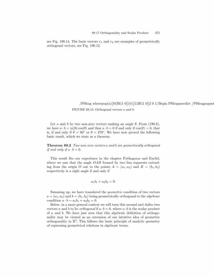
89.17 Orthogonality and Scalar Product 375
see Fig. 190.14. The basis vectors e1 and e2 are examples of geometricallyorthogonal vectors, see Fig. 190.12.
/PSfrag wherepop(a)[[0(Bl)1 0]](b)[[1(Bl)1 0]]2 0 1/Begin PSfraguserdict /PSfragpopputifelsea
b
/End PSfrag /Hide PSfragPSfrag replacements/Unhide PSfrag– a 0/Place PSfrag– b 1/Place PSfrag
FIGURE 89.13. Orthogonal vectors a and b.
Let a and b be two non-zero vectors making an angle θ. From (190.8),we have a · b = |a||b| cos(θ) and thus a · b = 0 if and only if cos(θ) = 0, thatis, if and only if θ = 90 or θ = 270. We have now proved the followingbasic result, which we state as a theorem.
Theorem 89.2 Two non-zero vectors a and b are geometrically orthogonalif and only if a · b = 0.
This result fits our experience in the chapter Pythagoras and Euclid,where we saw that the angle OAB formed by two line segments extend-ing from the origin O out to the points A = (a1, a2) and B = (b1, b2)respectively is a right angle if and only if
a1b1 + a2b2 = 0.
Summing up, we have translated the geometric condition of two vectorsa = (a1, a2) and b = (b1, b2) being geometrically orthogonal to the algebraiccondition a · b = a1b1 + a2b2 = 0.Below, in a more general context we will turn this around and define two
vectors a and b to be orthogonal if a · b = 0, where a · b is the scalar productof a and b. We have just seen that this algebraic definition of orthogo-nality may be viewed as an extension of our intuitive idea of geometricorthogonality in R2. This follows the basic principle of analytic geometryof expressing geometrical relations in algebraic terms.
376 89. Analytic Geometry in R2
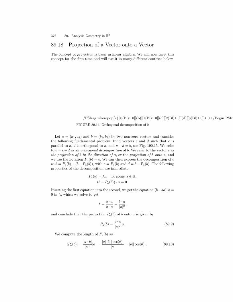
89.18 Projection of a Vector onto a Vector
The concept of projection is basic in linear algebra. We will now meet thisconcept for the first time and will use it in many different contexts below.
/PSfrag wherepop(a)[[0(Bl)1 0]](b)[[1(Bl)1 0]](c)[[2(Bl)1 0]](d)[[3(Bl)1 0]]4 0 1/Begin PSfraguserdict /PSfragpopputifelse
c
d
ab
/End PSfrag /Hide PSfragPSfrag replacements/Unhide PSfrag– a 0/Place PSfrag– b 1/Place PSfrag– c 2/Place PSfrag– d 3/Place PSfrag
FIGURE 89.14. Orthogonal decomposition of b
Let a = (a1, a2) and b = (b1, b2) be two non-zero vectors and considerthe following fundamental problem: Find vectors c and d such that c isparallel to a, d is orthogonal to a, and c+ d = b, see Fig. 190.15. We referto b = c+d as an orthogonal decomposition of b. We refer to the vector c asthe projection of b in the direction of a, or the projection of b onto a, andwe use the notation Pa(b) = c. We can then express the decomposition of bas b = Pa(b)+ (b−Pa(b)), with c = Pa(b) and d = b−Pa(b). The followingproperties of the decomposition are immediate:
Pa(b) = λa for some λ ∈ R,(b− Pa(b)) · a = 0.
Inserting the first equation into the second, we get the equation (b−λa)·a =0 in λ, which we solve to get
λ =b · aa · a
=b · a|a|2
,
and conclude that the projection Pa(b) of b onto a is given by
Pa(b) =b · a|a|2
a. (89.9)
We compute the length of Pa(b) as
|Pa(b)| =|a · b||a|2
|a| = |a| |b| | cos(θ)||a|
= |b|| cos(θ)|, (89.10)

89.18 Projection of a Vector onto a Vector 377
/PSfrag wherepop(a)[[0(Bl)1 0]](b)[[1(Bl)1 0]](theta)[[2(Bl)1 0]](Pb)[[3(Bl)1 0]](—Pb—=—b——cos(theta)—=—b.a—/—a—)[[4(Bl)1 0]]5 0 1/Begin PSfraguserdict /PSfragpopputifelse
|Pb|=|b||cos(theta)|=|b.a|/|a|
ab
Pbtheta
/End PSfrag /Hide PSfragPSfrag replacements/Unhide PSfrag– a 0/Place PSfrag– b 1/Place PSfrag– θ 2/Place PSfrag– Pa(b)˝ 3/Place PSfrag– |Pa(b)| = |b| | cos(θ)| = |b · a|/|a|˝ 4/Place PSfrag
FIGURE 89.15. The projection Pa(b) of b onto a.
where θ is the angle between a and b, and we use (190.8). We note that
|a · b| = |a| |Pb|, (89.11)
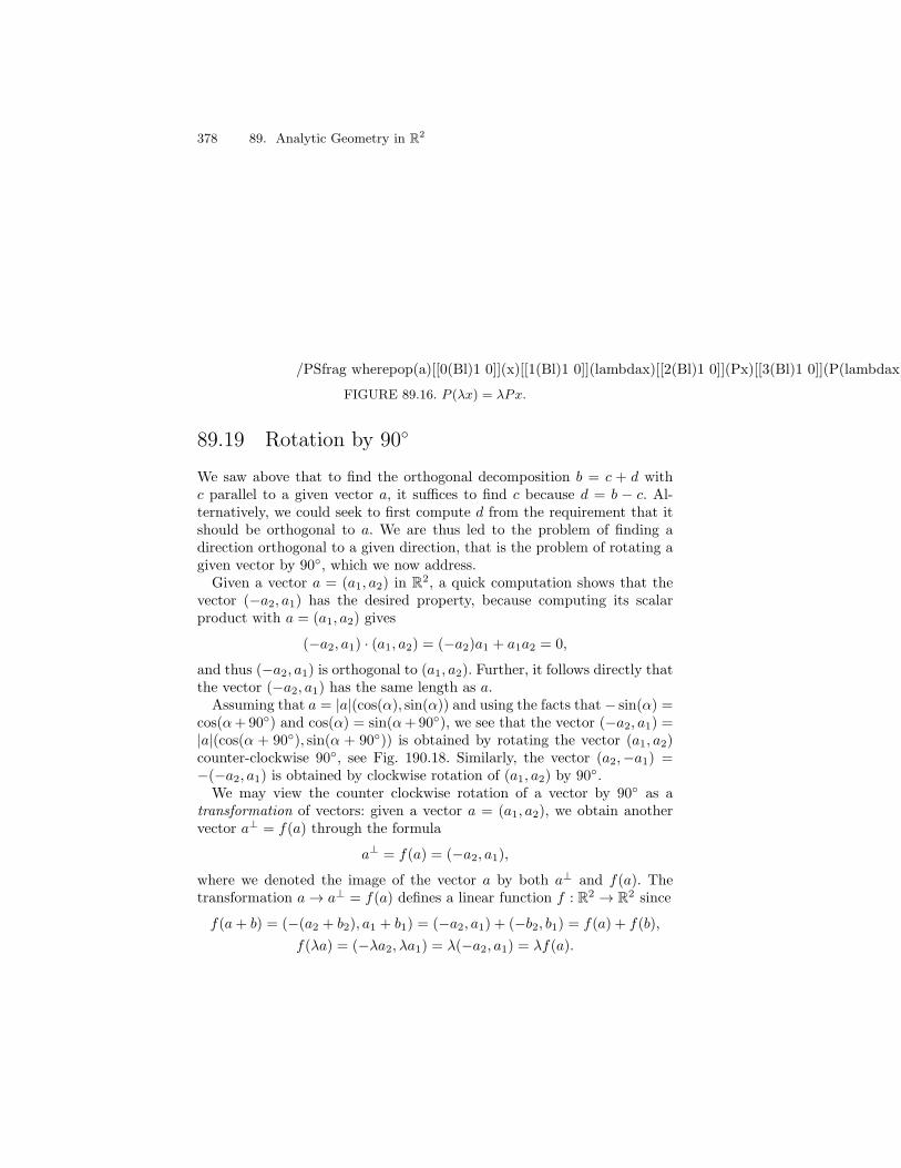
which conforms with our experience with the scalar product in Section190.16, see also Fig. 20.15.We can view the projection Pa(b) of the vector b onto the vector a as a
transformation of R2 into R2: given the vector b ∈ R2, we define the vectorPa(b) ∈ R2 by the formula
Pa(b) =b · a|a|2
a. (89.12)
We write for short Pb = Pa(b), suppressing the dependence on a and theparenthesis, and note that the mapping P : R2 → R2 defined by x → Pxis linear. We have
P (x+ y) = Px+ Py, P (λx) = λPx, (89.13)
for all x and y in R2 and λ ∈ R (where we changed name of the independentvariable from b to x or y), see Fig. 190.17.We note that P (Px) = Px for all x ∈ R2. This could also be expressed
as P 2 = P , which is a characteristic property of a projection. Projecting asecond time doesn’t change anything!We sum up:
Theorem 89.3 The projection x → Px = Pa(x) onto a given nonzerovector a ∈ R2 is a linear mapping P : R2 → R2 with the property thatPP = P .
Example 89.6. If a = (1, 3) and b = (5, 2), then Pa(b) =(1,3)·(5,2)
1+32 (1, 3)= (1.1, 3.3).
378 89. Analytic Geometry in R2
/PSfrag wherepop(a)[[0(Bl)1 0]](x)[[1(Bl)1 0]](lambdax)[[2(Bl)1 0]](Px)[[3(Bl)1 0]](P(lambdax)=lambdaPx)[[4(Bl)1 0]]5 0 1/Begin PSfraguserdict /PSfragpopputifelse
x
a
Px
lambdax
P(lambdax)=lambdaPx
/End PSfrag /Hide PSfragPSfrag replacements/Unhide PSfrag– a 0/Place PSfrag– x 1/Place PSfrag– λx2/Place PSfrag– P x3/Place PSfrag– P (λx) = λPx˝ 4/Place PSfrag
FIGURE 89.16. P (λx) = λPx.
89.19 Rotation by 90
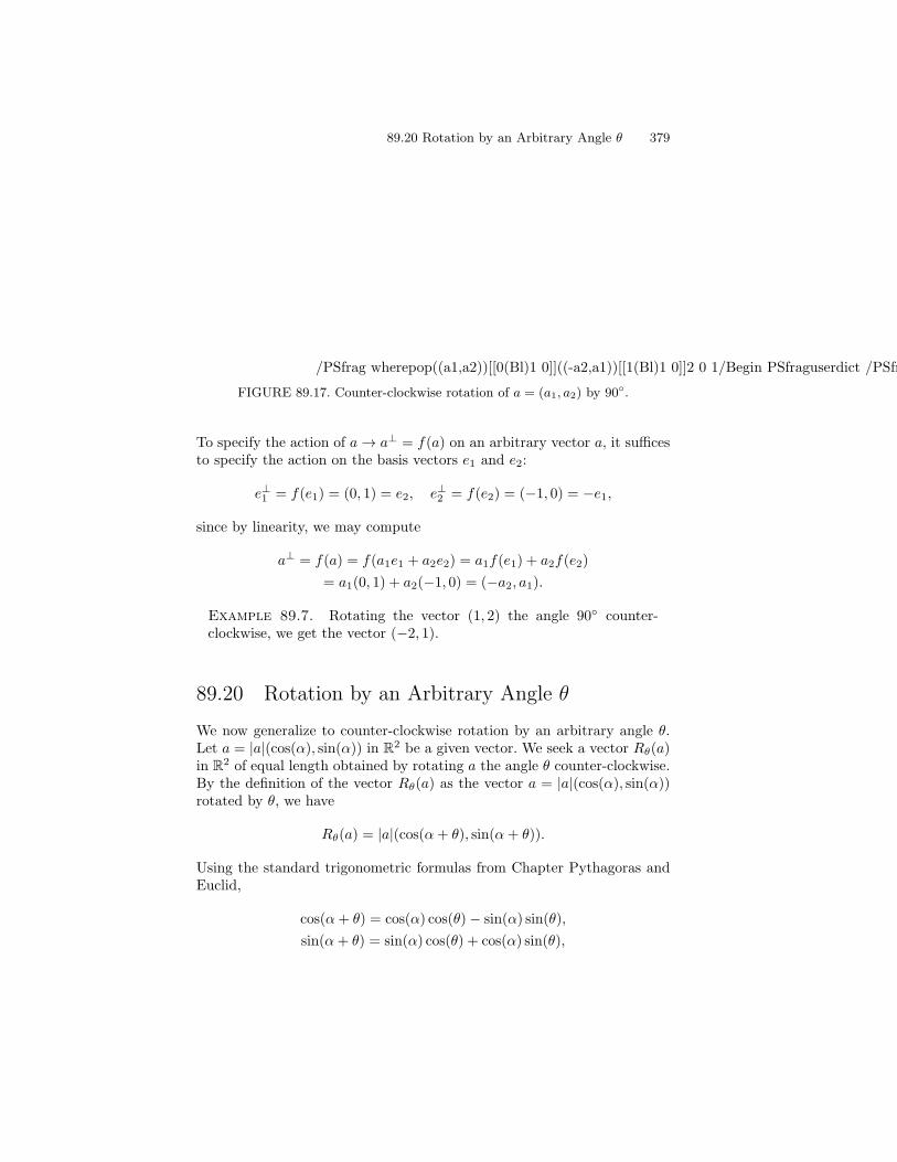
We saw above that to find the orthogonal decomposition b = c + d withc parallel to a given vector a, it suffices to find c because d = b − c. Al-ternatively, we could seek to first compute d from the requirement that itshould be orthogonal to a. We are thus led to the problem of finding adirection orthogonal to a given direction, that is the problem of rotating agiven vector by 90, which we now address.Given a vector a = (a1, a2) in R2, a quick computation shows that the
vector (−a2, a1) has the desired property, because computing its scalarproduct with a = (a1, a2) gives
(−a2, a1) · (a1, a2) = (−a2)a1 + a1a2 = 0,
and thus (−a2, a1) is orthogonal to (a1, a2). Further, it follows directly thatthe vector (−a2, a1) has the same length as a.Assuming that a = |a|(cos(α), sin(α)) and using the facts that − sin(α) =
cos(α+90) and cos(α) = sin(α+90), we see that the vector (−a2, a1) =|a|(cos(α + 90), sin(α + 90)) is obtained by rotating the vector (a1, a2)counter-clockwise 90, see Fig. 190.18. Similarly, the vector (a2,−a1) =−(−a2, a1) is obtained by clockwise rotation of (a1, a2) by 90.We may view the counter clockwise rotation of a vector by 90 as a
transformation of vectors: given a vector a = (a1, a2), we obtain anothervector a⊥ = f(a) through the formula
a⊥ = f(a) = (−a2, a1),
where we denoted the image of the vector a by both a⊥ and f(a). Thetransformation a → a⊥ = f(a) defines a linear function f : R2 → R2 since
f(a+ b) = (−(a2 + b2), a1 + b1) = (−a2, a1) + (−b2, b1) = f(a) + f(b),
f(λa) = (−λa2, λa1) = λ(−a2, a1) = λf(a).
89.20 Rotation by an Arbitrary Angle θ 379
/PSfrag wherepop((a1,a2))[[0(Bl)1 0]]((-a2,a1))[[1(Bl)1 0]]2 0 1/Begin PSfraguserdict /PSfragpopputifelse
(a1,a2)
(−a2,a1)
/End PSfrag /Hide PSfragPSfrag replacements/Unhide PSfrag– (a1, a2)˝ 0/Place PSfrag– (−a2, a1)˝ 1/Place PSfrag
FIGURE 89.17. Counter-clockwise rotation of a = (a1, a2) by 90.
To specify the action of a → a⊥ = f(a) on an arbitrary vector a, it sufficesto specify the action on the basis vectors e1 and e2:
e⊥1 = f(e1) = (0, 1) = e2, e⊥2 = f(e2) = (−1, 0) = −e1,
since by linearity, we may compute
a⊥ = f(a) = f(a1e1 + a2e2) = a1f(e1) + a2f(e2)
= a1(0, 1) + a2(−1, 0) = (−a2, a1).
Example 89.7. Rotating the vector (1, 2) the angle 90 counter-clockwise, we get the vector (−2, 1).
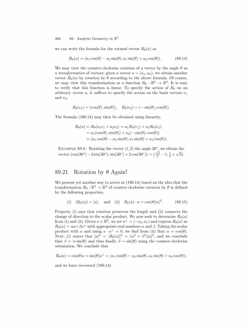
89.20 Rotation by an Arbitrary Angle θ
We now generalize to counter-clockwise rotation by an arbitrary angle θ.Let a = |a|(cos(α), sin(α)) in R2 be a given vector. We seek a vector Rθ(a)in R2 of equal length obtained by rotating a the angle θ counter-clockwise.By the definition of the vector Rθ(a) as the vector a = |a|(cos(α), sin(α))rotated by θ, we have
Rθ(a) = |a|(cos(α+ θ), sin(α+ θ)).
Using the standard trigonometric formulas from Chapter Pythagoras andEuclid,
cos(α+ θ) = cos(α) cos(θ)− sin(α) sin(θ),
sin(α+ θ) = sin(α) cos(θ) + cos(α) sin(θ),
380 89. Analytic Geometry in R2
we can write the formula for the rotated vector Rθ(a) as
Rθ(a) = (a1 cos(θ)− a2 sin(θ), a1 sin(θ) + a2 cos(θ)). (89.14)
We may view the counter-clockwise rotation of a vector by the angle θ asa transformation of vectors: given a vector a = (a1, a2), we obtain anothervector Rθ(a) by rotation by θ according to the above formula. Of course,we may view this transformation as a function Rθ : R2 → R2. It is easyto verify that this function is linear. To specify the action of Rθ on anarbitrary vector a, it suffices to specify the action on the basis vectors e1and e2,
Rθ(e1) = (cos(θ), sin(θ)), Rθ(e2) = (− sin(θ), cos(θ)).
The formula (190.14) may then be obtained using linearity,
Rθ(a) = Rθ(a1e1 + a2e2) = a1Rθ(e1) + a2Rθ(e2)
= a1(cos(θ), sin(θ)) + a2(− sin(θ), cos(θ))
= (a1 cos(θ)− a2 sin(θ), a1 sin(θ) + a2 cos(θ)).
Example 89.8. Rotating the vector (1, 2) the angle 30, we obtain the
vector (cos(30)− 2 sin(30), sin(30) + 2 cos(30)) = (√32 − 1, 1
2 +√3).
89.21 Rotation by θ Again!
We present yet another way to arrive at (190.14) based on the idea that thetransformation Rθ : R2 → R2 of counter-clockwise rotation by θ is definedby the following properties,
(i) |Rθ(a)| = |a|, and (ii) Rθ(a) · a = cos(θ)|a|2. (89.15)
Property (i) says that rotation preserves the length and (ii) connects thechange of direction to the scalar product. We now seek to determine Rθ(a)from (i) and (ii). Given a ∈ R2, we set a⊥ = (−a2, a1) and express Rθ(a) asRθ(a) = αa+βa⊥ with appropriate real numbers α and β. Taking the scalarproduct with a and using a · a⊥ = 0, we find from (ii) that α = cos(θ).Next, (i) states that |a|2 = |Rθ(a)|2 = (α2 + β2)|a|2, and we concludethat β = ± sin(θ) and thus finally β = sin(θ) using the counter-clockwiseorientation. We conclude that
Rθ(a) = cos(θ)a+ sin(θ)a⊥ = (a1 cos(θ)− a2 sin(θ), a1 sin(θ) + a2 cos(θ)),
and we have recovered (190.14).

89.22 Rotating a Coordinate System 381
89.22 Rotating a Coordinate System
Suppose we rotate the standard basis vectors e1 = (1, 0) and e2 = (0, 1)counter-clockwise the angle θ to get the new vectors e1 = cos(θ)e1+sin(θ)e2and e2 = − sin(θ)e1+cos(θ)e2. We may use e1 and e2 as an alternative co-ordinate system, and we may seek the connection between the coordinatesof a given vector (or point) in the old and new coordinate system. Letting(a1, a2) be the coordinates in the standard basis e1 and e2, and (a1, a2) thecoordinates in the new basis e1 and e2, we have
a1e1 + a2e2 = a1e1 + a2e2
= a1(cos(θ)e1 + sin(θ)e2) + a2(− sin(θ)e1 + cos(θ)e2)
= (a1 cos(θ)− a2 sin(θ))e1 + (a1 sin(θ) + a2 cos(θ))e2,
so the uniqueness of coordinates with respect to e1 and e2 implies
a1 = cos(θ)a1 − sin(θ)a2,
a2 = sin(θ)a1 + cos(θ)a2.(89.16)
Since e1 and e2 are obtained by rotating e1 and e2 clockwise by the angleθ,
a1 = cos(θ)a1 + sin(θ)a2,
a2 = − sin(θ)a1 + cos(θ)a2.(89.17)
The connection between the coordinates with respect to the two coordinatesystems is thus given by (190.16) and (190.17).
Example 89.9. Rotating 45 counter-clockwise gives the followingrelation between new and old coordinates
a1 =1√2(a1 + a2), a2 =
1√2(−a1 + a2).
89.23 Vector Product
We now define the vector product a × b of two vectors a = (a1, a2) andb = (b1, b2) in R2 by the formula
a× b = a1b2 − a2b1. (89.18)
The vector product a× b is also referred to as the cross product because ofthe notation used (don’t mix up with the “×” in the “product set” R2×R2
which has a different meaning). The vector product or cross product maybe viewed as a function R2 × R2 → R. This function is bilinear as is easyto verify, and anti-symmetric, that is
a× b = −b× a, (89.19)
382 89. Analytic Geometry in R2
which is a surprising property for a product.Since the vector product is bilinear, we can specify the action of the
vector product on two arbitrary vectors a and b by specifying the actionon the basis vectors,
e1 × e1 = 0, e2 × e2 = 0, e1 × e2 = 1, e2 × e1 = −1. (89.20)
Using these relations,
a×b = (a1e1+a2e2)×(b1e1+b2e2) = a1b2e1×e2+a2b1e2×e1 = a1b2−a2b1e2.
We next show that the properties of bilinearity and anti-symmetry infact determine the vector product in R2 up to a constant. First note thatanti-symmetry and bilinearity imply
e1 × e1 + e1 × e2 = e1 × (e1 + e2) = −(e1 + e2)× e1
= −e1 × e1 − e2 × e1.
Since e1 × e2 = −e2 × e1, we have e1 × e1 = 0. Similarly, we see thate2×e2 = 0. We conclude that the action of the vector product on the basisvectors is indeed specified according to (190.20) up to a constant.We next observe that
a× b = (−a2, a1) · (b1, b2) = a1b2 − a2b1,
which gives a connection between the vector product a × b and the scalarproduct a⊥ ·b with the 90 counter-clockwise rotated vector a⊥ = (−a2, a1).We conclude that the vector product a × b of two nonzero vectors a andb is zero if and only if a and b are parallel. We state this basic result as atheorem.
Theorem 89.4 Two nonzero vectors a and b are parallel if and only ifa× b = 0.
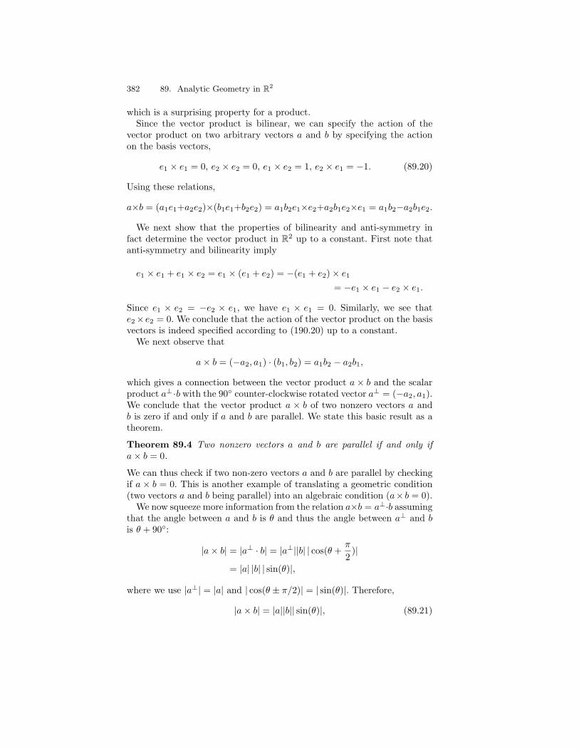
We can thus check if two non-zero vectors a and b are parallel by checkingif a × b = 0. This is another example of translating a geometric condition(two vectors a and b being parallel) into an algebraic condition (a× b = 0).We now squeeze more information from the relation a×b = a⊥·b assuming
that the angle between a and b is θ and thus the angle between a⊥ and bis θ + 90:
|a× b| = |a⊥ · b| = |a⊥||b| | cos(θ + π
2)|
= |a| |b| | sin(θ)|,
where we use |a⊥| = |a| and | cos(θ ± π/2)| = | sin(θ)|. Therefore,
|a× b| = |a||b|| sin(θ)|, (89.21)
89.23 Vector Product 383
/PSfrag wherepop(a)[[0(Bl)1 0]](b)[[1(Bl)1 0]](theta)[[2(Bl)1 0]]((-a2,a1))[[3(Bl)1 0]]4 0 1/Begin PSfraguserdict /PSfragpopputifelse
(−a2,a1)
b
a
theta
/End PSfrag /Hide PSfragPSfrag replacements/Unhide PSfrag– a 0/Place PSfrag– b 1/Place PSfrag– θ 2/Place PSfrag– (−a2, a1)˝ 3/Place PSfrag
FIGURE 89.18. Why |a× b| = |a| |b| | sin(θ)|.
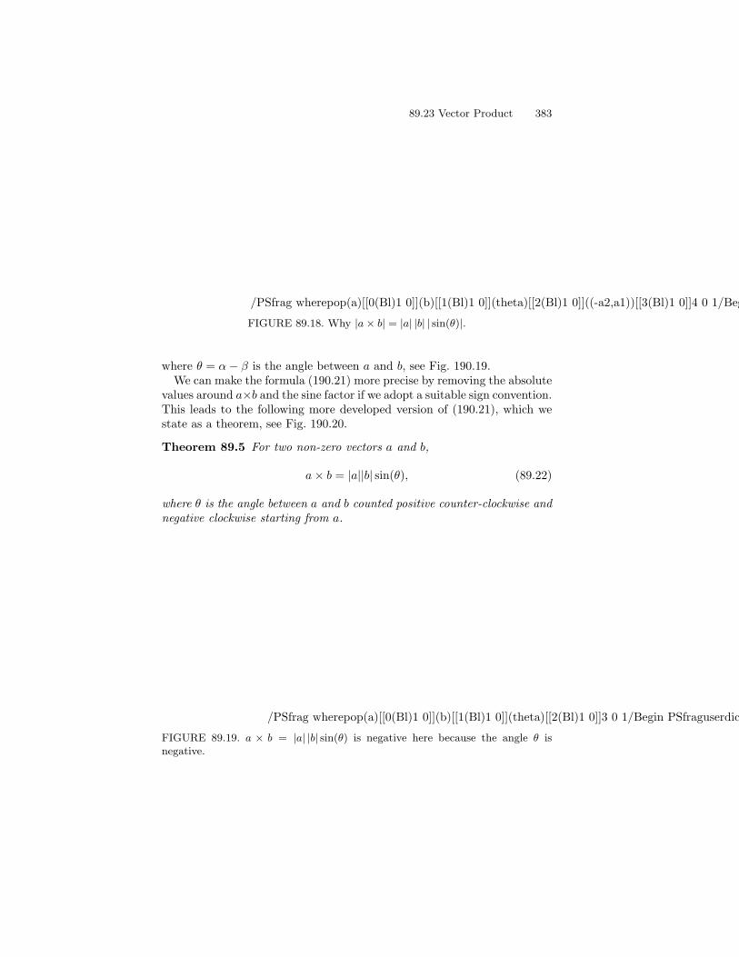
where θ = α− β is the angle between a and b, see Fig. 190.19.We can make the formula (190.21) more precise by removing the absolute
values around a×b and the sine factor if we adopt a suitable sign convention.This leads to the following more developed version of (190.21), which westate as a theorem, see Fig. 190.20.
Theorem 89.5 For two non-zero vectors a and b,
a× b = |a||b| sin(θ), (89.22)
where θ is the angle between a and b counted positive counter-clockwise andnegative clockwise starting from a.
/PSfrag wherepop(a)[[0(Bl)1 0]](b)[[1(Bl)1 0]](theta)[[2(Bl)1 0]]3 0 1/Begin PSfraguserdict /PSfragpopputifelse
a
btheta
/End PSfrag /Hide PSfragPSfrag replacements/Unhide PSfrag– a 0/Place PSfrag– b 1/Place PSfrag– θ 2/Place PSfrag
FIGURE 89.19. a × b = |a| |b| sin(θ) is negative here because the angle θ isnegative.

384 89. Analytic Geometry in R2
89.24 The Area of a Triangle with a Corner at theOrigin
Consider a triangle OAB with corners at the origin O and the points A =(a1, a2) and B = (b1, b2) formed by the vectors a = (a1, a2) and b = (b1, b2),see Fig. 190.21. We say that the triangle OAB is spanned by the vectors aand b. We are familiar with the formula that states that the area of thistriangle can be computed as the base |a| times the height |b|| sin(θ)| timesthe factor 1
2 , where θ is the angle between a and b, see Fig. 190.21. Recalling(190.21), we conclude
Theorem 89.6
Area(OAB) =1
2|a| |b| | sin(θ)| = 1
2|a× b|.
/PSfrag wherepop(theta)[[0(Bl)1 0]](a)[[1(Bl)1 0]](b)[[2(Bl)1 0]](A)[[3(Bl)1 0]](B)[[4(Bl)1 0]](O)[[5(Bl)1 0]](—b—sin(theta))[[6(Bl)1 0]]7 0 1/Begin PSfraguserdict /PSfragpopputifelse
b
a
A
B
theta
|b|sin(theta)
O
/End PSfrag /Hide PSfragPSfrag replacements/Unhide PSfrag– θ 0/Place PSfrag– a 1/Place PSfrag– b 2/Place PSfrag– A 3/Place PSfrag– B 4/Place PSfrag– O 5/Place PSfrag– |b| sin(θ)˝ 6/Place PSfrag
FIGURE 89.20. The vectors a and b span a triangle with area 12|a× b|.
The area of the triangle OAB can be computed using the vector productin R2.
89.25 The Area of a General Triangle
Consider a triangle CAB with corners at the points C = (c1, c2), A =(a1, a2) and B = (b1, b2). We consider the problem of computing the areaof the triangle CAB. We solved this problem above in the case C = Owhere O is the origin. We may reduce the present case to that case bychanging coordinate system as follows. Consider a new coordinate systemwith origin at C = (c1, c2) and with a x1-axis parallel to the x1-axis and ax2-axis parallel to the x2-axis, see Fig. 190.22.

89.26 The Area of a Parallelogram Spanned by Two Vectors 385
/PSfrag wherepop(O)[[0(Bl)1 0]](x1)[[1(Bl)1 0]](x2)[[2(Bl)1 0]](hatx1)[[3(Bl)1 0]](hatx2)[[4(Bl)1 0]](a-c)[[5(Bl)1 0]](b-c)[[6(Bl)1 0]](C=(c1,c2))[[7(Bl)1 0]](A=(a1,a2))[[8(Bl)1 0]](B=(b1,b2))[[9(Bl)1 0]](theta)[[10(Bl)1 0]]11 0 1/Begin PSfraguserdict /PSfragpopputifelse
a−c
x1
x2
hatx1
hatx2
theta A=(a1,a2)
B=(b1,b2)
C=(c1,c2)
b−c
O
/End PSfrag /Hide PSfragPSfrag replacements/Unhide PSfrag– O 0/Place PSfrag– x1 1/Place PSfrag– x2 2/Place PSfrag– x1 3/Place PSfrag– x2 4/Place PSfrag– a−c˝ 5/Place PSfrag– b−c˝ 6/Place PSfrag– C = (c1, c2)˝ 7/Place PSfrag– A = (a1, a2)˝ 8/Place PSfrag– B = (b1, b2)˝ 9/Place PSfrag– θ 10/Place PSfrag
FIGURE 89.21. Vectors a−c and b−c span triangle with area 12|(a−c)×(b−c)|.
Letting (a1, a2) denote the coordinates with respect to the new coordi-nate system, the new are related to the old coordinates by
a1 = a1 − c1, a2 = a2 − c2.
The coordinates of the points A, B and C in the new coordinate systemare thus (a1− c1, a2− c2) = a− c, (b1− c1, b2− c2) = b− c and (0, 0). Usingthe result from the previous section, we find the area of the triangle CABby the formula
Area(CAB) =1
2|(a− c)× (b− c)|. (89.23)
Example 89.10. The area of the triangle with coordinates at A =(2, 3), B = (−2, 2) and C = (1, 1), is given by Area(CAB) = 1
2 |(1, 2)×(−3, 1)| = 7
2 .
89.26 The Area of a Parallelogram Spanned byTwo Vectors
The area of the parallelogram spanned by a and b, as shown in Fig. 190.23,is equal to |a × b| since the area of the parallelogram is twice the area ofthe triangle spanned by a and b. Denoting the area of the parallelogramspanned by the vectors a and b by V (a, b), we thus have the formula
V (a, b) = |a× b|. (89.24)
This is a fundamental formula which has important generalizations to R3
and Rn.

386 89. Analytic Geometry in R2
/PSfrag wherepop(a)[[0(Bl)1 0]](b)[[1(Bl)1 0]](theta)[[2(Bl)1 0]](—b—sin(theta))[[3(Bl)1 0]]4 0 1/Begin PSfraguserdict /PSfragpopputifelse
b
atheta
|b|sin(theta)
/End PSfrag /Hide PSfragPSfrag replacements/Unhide PSfrag– a 0/Place PSfrag– b 1/Place PSfrag– θ 2/Place PSfrag– |b| sin(θ)˝ 3/Place PSfrag
FIGURE 89.22. The vectors a and b span a rectangle with area|a× b| = |a| |b| sin(θ)|.
89.27 Straight Lines
The points x = (x1, x2) in the plane R2 satisfying a relation of the form
n1x1 + n2x2 = n · x = 0, (89.25)
where n = (n1, n2) ∈ R2 is a given non-zero vector, form a straight linethrough the origin that is orthogonal to (n1, n2), see Fig. 190.24. We saythat (n1, n2) is a normal to the line. We can represent the points x ∈ R2
on the line in the formx = sn⊥, s ∈ R,
where n⊥ = (−n2, n1) is orthogonal to n, see Fig. 190.24. We state thisinsight as a theorem because of its importance.
Theorem 89.7 A line in R2 passing through the origin with normal n ∈R2, may be expressed as either the points x ∈ R2 satisfying n · x = 0, orthe set of points of the form x = sn⊥ with n⊥ ∈ R2 orthogonal to n ands ∈ R.
Similarly, the set of points (x1, x2) in R2 such that
n1x1 + n2x2 = d, (89.26)
where n = (n1, n2) ∈ R2 is a given non-zero vector and d is a given constant,represents a straight line that does not pass through the origin if d = 0.We see that n is a normal to the line, since if x and x are two points onthe line then (x − x) · n = d − d = 0, see Fig. 190.25. We may define theline as the points x = (x1, x2) in R2, such that the projection n·x
|n|2n of the
vector x = (x1, x2) in the direction of n is equal to d|n|2n. To see this, we
use the definition of the projection and the fact n · x = d.

89.27 Straight Lines 387
/PSfrag wherepop(x)[[0(Bl)1 0]](n)[[1(Bl)1 0]](x1)[[2(Bl)1 0]](x2)[[3(Bl)1 0]](nperp)[[4(Bl)1 0]](x=snperp)[[5(Bl)1 0]]6 0 1/Begin PSfraguserdict /PSfragpopputifelse
x2
x1
x2
x2
nperp x=snperp
nn
x
/End PSfrag /Hide PSfragPSfrag replacements/Unhide PSfrag– x 0/Place PSfrag– n 1/Place PSfrag– x1 2/Place PSfrag– x2 3/Place PSfrag– n⊥4/Place PSfrag– x = sn⊥˝ 5/Place PSfrag
FIGURE 89.23. Vectors x = sa with b orthogonal to a given vector n generate aline through the origin with normal a.
The line in Fig. 190.24 can also be represented as the set of points
x = x+ sn⊥ s ∈ R,
where x is any point on the line (thus satisfying n · x = d). This is becauseany point x of the form x = sn⊥ + x evidently satisfies n · x = n · x = d.We sum up in the following theorem.
Theorem 89.8 The set of points x ∈ R2 such that n ·x = d, where n ∈ R2
is a given non-zero vector and d is given constant, represents a straight linein R2. The line can also be expressed in the form x = x + sn⊥ for s ∈ R,where x ∈ R2 is a point on the line.
/PSfrag wherepop(O)[[0(Bl)1 0]](x1)[[1(Bl)1 0]](x2)[[2(Bl)1 0]](n)[[3(Bl)1 0]](nperp)[[4(Bl)1 0]](hatx)[[5(Bl)1 0]](x=(x1,x2))[[6(Bl)1 0]]7 0 1/Begin PSfraguserdict /PSfragpopputifelse
Ox1
x2
x=(x1,x2)
n
hatx
nperp
/End PSfrag /Hide PSfragPSfrag replacements/Unhide PSfrag– O 0/Place PSfrag– x1 1/Place PSfrag– x2 2/Place PSfrag– n 3/Place PSfrag– n⊥4/Place PSfrag– x 5/Place PSfrag– x = (x1, x2)˝ 6/Place PSfrag
FIGURE 89.24. The line through the point x with normal n generated by direc-tional vector a.

388 89. Analytic Geometry in R2
Example 89.11. The line x1+2x2 = 3 can alternatively be expressedas the set of points x = (1, 1) + s(−2, 1) with s ∈ R.
89.28 Projection of a Point onto a Line
Let n · x = d represent a line in R2 and let b be a point in R2 that doesnot lie on the line. We consider the problem of finding the point Pb on theline which is closest to b, see Fig. 190.27. This is called the projection ofthe point b onto the line. Equivalently, we seek a point Pb on the line suchthat b− Pb is orthogonal to the line, that is we seek a point Pb such that
n · Pb = d (Pb is a point on the line),
b− Pb is parallel to the normal n, (b− Pb = λn, for some λ ∈ R).
We conclude that Pb = b − λn and the equation n · Pb = d thus givesn · (b− λn) = d, that is λ = b·n−d
|n|2 and so
Pb = b− b · n− d
|n|2n. (89.27)
If d = 0, that is the line n · x = d = 0 passes through the origin, then (seeProblem 190.26)
Pb = b− b · n|n|2
n. (89.28)
89.29 When Are Two Lines Parallel?
Leta11x1 + a12x2 = b1,a21x1 + a22x2 = b2,
be two straight lines in R2 with normals (a11, a12) and (a21, a22). How dowe know if the lines are parallel? Of course, the lines are parallel if andonly if their normals are parallel. From above, we know the normals areparallel if and only if
(a11, a12)× (a21, a22) = a11a22 − a12a21 = 0,
and consequently non-parallel (and consequently intersecting at somepoint) if and only if
(a11, a12)× (a21, a22) = a11a22 − a12a21 = 0, (89.29)
Example 89.12. The two lines 2x1 + 3x2 = 1 and 3x1 + 4x2 = 1 arenon-parallel because 2 · 4− 3 · 3 = 8− 9 = −1 = 0.
89.30 A System of Two Linear Equations in Two Unknowns 389
89.30 A System of Two Linear Equations in TwoUnknowns
If a11x1 + a12x2 = b1 and a21x1 + a22x2 = b2 are two straight lines in R2
with normals (a11, a12) and (a21, a22), then their intersection is determinedby the system of linear equations
a11x1 + a12x2 = b1,a21x1 + a22x2 = b2,
(89.30)
which says that we seek a point (x1, x2) ∈ R2 that lies on both lines. Thisis a system of two linear equations in two unknowns x1 and x2, or a 2× 2-system. The numbers aij , i, j = 1, 2 are the coefficients of the system andthe numbers bi, i = 1, 2, represent the given right hand side.If the normals (a11, a12) and (a21, a22) are not parallel or by (190.29),
a11a22 − a12a21 = 0, then the lines must intersect and thus the system(190.30) should have a unique solution (x1, x2). To determine x1, we mul-tiply the first equation by a22 to get
a11a22x1 + a12a22x2 = b1a22.
We then multiply the second equation by a12, to get
a21a12x1 + a22a12x2 = b2a12.
Subtracting the two equations the x2-terms cancel and we get the followingequation containing only the unknown x1,
a11a22x1 − a21a12x1 = b1a22 − b2a12.
Solving for x1, we get
x1 = (a22b1 − a12b2)(a11a22 − a12a21)−1.
Similarly to determine x2, we multiply the first equation by a21 and sub-tract the second equation multiplied by a11, which eliminates a1. Alto-gether, we obtain the solution formula
x1 = (a22b1 − a12b2)(a11a22 − a12a21)−1, (89.31a)
x2 = (a11b2 − a21b1)(a11a22 − a12a21)−1. (89.31b)
This formula gives the unique solution of (190.30) under the conditiona11a22 − a12a21 = 0.We can derive the solution formula (190.31) in a different way, still as-
suming that a11a22 − a12a21 = 0. We define a1 = (a11, a21) and a2 =(a12, a22), noting carefully that here a1 and a2 denote vectors and that

390 89. Analytic Geometry in R2
a1×a2 = a11a22−a12a21 = 0, and rewrite the two equations of the system(190.30) in vector form as
x1a1 + x2a2 = b. (89.32)
Taking the vector product of this equation with a2 and a1 and using a2 ×a2 = a1 × a1 = 0,
x1a1 × a2 = b× a2, x2a2 × a1 = b× a1.
Since a1 × a2 = 0,
x1 =b× a2a1 × a2
, x2 =b× a1a2 × a1
= − b× a1a1 × a2
, (89.33)
which agrees with the formula (190.31) derived above.We conclude this section by discussing the case when a1×a2 = a11a22−
a12a21 = 0, that is the case when a1 and a2 are parallel or equivalentlythe two lines are parallel. In this case, a2 = λa1 for some λ ∈ R andthe system (190.30) has a solution if and only if b2 = λb1, since then thesecond equation results from multiplying the first by λ. In this case thereare infinitely many solutions since the two lines coincide. In particular ifwe choose b1 = b2 = 0, then the solutions consist of all (x1, x2) such thata11x1 + a12x2 = 0, which defines a straight line through the origin. Onthe other hand if b2 = λb1, then the two equations represent two differentparallel lines that do not intersect and there is no solution to the system(190.30).We summarize our experience from this section on systems of 2 linear
equations in 2 unknowns as follows:
Theorem 89.9 The system of linear equations x1a1 + x2a2 = b, wherea1, a2 and b are given vectors in R2, has a unique solution (x1, x2) given by(190.33) if a1 × a2 = 0. In the case a1 × a2 = 0, the system has no solutionor infinitely many solutions, depending on b.
Below we shall generalize this result to systems of n linear equations in nunknowns, which represents one of the most basic results of linear algebra.
Example 89.13. The solution to the system
x1 + 2x2 = 3,4x1 + 5x2 = 6,
is given by
x1 =(3, 6)× (2, 5)
(1, 4)× (2, 5)=
3
−3= −1, x2 = − (3, 6)× (1, 4)
(1, 4)× (2, 5)= − 6
−3= 2.

89.31 Linear Independence and Basis 391
89.31 Linear Independence and Basis
We saw above that the system (190.30) can be written in vector form as
x1a1 + x2a2 = b,
where b = (b1, b2), a1 = (a11, a21) and a2 = (a12, a22) are all vectors in R2,and x1 and x2 real numbers. We say that
x1a1 + x2a2,
is a linear combination of the vectors a1 and a2, or a linear combinationof the set of vectors a1, a2, with the coefficients x1 and x2 being realnumbers. The system of equations (190.30) expresses the right hand sidevector b as a linear combination of the set of vectors a1, a2 with thecoefficients x1 and x2. We refer to x1 and x2 as the coordinates of b withrespect to the set of vectors a1, a2, which we may write as an orderedpair (x1, x2).The solution formula (190.33) thus states that if a1 × a2 = 0, then an
arbitrary vector b in R2 can be expressed as a linear combination of theset of vectors a1, a2 with the coefficients x1 and x2 being uniquely deter-mined. This means that if a1 × a2 = 0, then the the set of vectors a1, a2may serve as a basis for R2, in the sense that each vector b in R2 may beuniquely expressed as a linear combination b = x1a1+x2a2 of the set of vec-tors a1, a2. We say that the ordered pair (x1, x2) are the coordinates of bwith respect to the basis a1, a2. The system of equations b = x1a1+x2a2thus give the coupling between the coordinates (b1, b2) of the vector b inthe standard basis, and the coordinates (x1, x2) with respect to the basisa1, a2. In particular, if b = 0 then x1 = 0 and x2 = 0.Conversely if a1×a2 = 0, that is a1 and a2 are parallel, then any nonzero
vector b orthogonal to a1 is also orthogonal to a2 and b cannot be expressedas b = x1a1 + x2a2. Thus, if a1 × a2 = 0 then a1, a2 cannot serve as abasis. We have now proved the following basic theorem:
Theorem 89.10 A set a1, a2 of two non-zero vectors a1 and a2 mayserve as a basis for R2 if and only if if a1 × a2 = 0. The coordinates(b1, b2) of a vector b in the standard basis and the coordinates (x1, x2) of bwith respect to a basis a1, a2 are related by the system of linear equationsb = x1a1 + x2a2.
Example 89.14. The two vectors a1 = (1, 2) and a2 = (2, 1) (expressedin the standard basis) form a basis for R2 since a1 × a2 = 1− 4 = −3.Let b = (5, 4) in the standard basis. To express b in the basis a1, a2,we seek real numbers x1 and x2 such that b = x1a1 + x2a2, and usingthe solution formula (190.33) we find that x1 = 1 and x2 = 2. Thecoordinates of b with respect to the basis a1, a2 are thus (1, 2), whilethe coordinates of b with respect to the standard basis are (5, 4).

392 89. Analytic Geometry in R2
We next introduce the concept of linear independence, which will playan important role below. We say that a set a1, a2 of two non-zero vectorsa1 and a2 two non-zero vectors a1 and a2 in R2 is linearly independent ifthe system of equations
x1a1 + x2a2 = 0
has the unique solution x1 = x2 = 0. We just saw that if a1 × a2 = 0, thena1 and a2 are linearly independent (because b = (0, 0) implies x1 = x2 = 0).Conversely if a1 × a2 = 0, then a1 and a2 are parallel so that a1 = λa2 forsome λ = 0, and then there are many possible choices of x1 and x2, notboth equal to zero, such that x1a1 + x2a2 = 0, for example x1 = −1 andx2 = λ. We have thus proved:
Theorem 89.11 The set a1, a2 of non-zero vectors a1 and a2 is linearlyindependent if and only if a1 × a2 = 0.
/PSfrag wherepop(x1)[[0(Bl)1 0]](x2)[[1(Bl)1 0]](c1)[[2(Bl)1 0]](c2)[[3(Bl)1 0]](c=0.73c1+1.7c2)[[4(Bl)1 0]]5 0 1/Begin PSfraguserdict /PSfragpopputifelse
c2
c1
x1
x2
c=0.73c1+1.7c2
/End PSfrag /Hide PSfragPSfrag replacements/Unhide PSfrag– x1 0/Place PSfrag– x2 1/Place PSfrag– c1 2/Place PSfrag– c2 3/Place PSfrag– c = 0.73c1 + 1.7c2˝ 4/Place PSfrag
FIGURE 89.25. Linear combination c of two linearly independent vectors c1 andc2
89.32 The Connection to Calculus in One Variable
We have discussed Calculus of real-valued functions y = f(x) of one realvariable x ∈ R, and we have used a coordinate system in R2 to plot graphsof functions y = f(x) with x and y representing the two coordinate axis.Alternatively, we may specify the graph as the set of points (x1, x2) ∈ R2,consisting of pairs (x1, x2) of real numbers x1 and x2, such that x2 = f(x1)or x2 − f(x1) = 0 with x1 representing x and x2 representing y. We referto the ordered pair (x1, x2) ∈ R2 as a vector x = (x1, x2) with componentsx1 and x2.

89.33 Linear Mappings f : R2 → R 393
We have also discussed properties of linear functions f(x) = ax + b,where a and b are real constants, the graphs of which are straight linesx2 = ax1+ b in R2. More generally, a straight line in R2 is the set of points(x1, x2) ∈ R2 such that x1a1 + x2a2 = b, where the a1, a2 and b are realconstants, with a1 = 0 and/or a2 = 0. We have noticed that (a1, a2) maybe viewed as a direction in R2 that is perpendicular or normal to the linea1x1 + a2x2 = b, and that (b/a1, 0) or (0, b/a2) are the points where theline intersects the x1-axis and the x2-axis respectively.
89.33 Linear Mappings f : R2 → RA function f : R2 → R is linear if for any x = (x1, x2) and y = (y1, y2) inR2 and any λ in R,
f(x+ y) = f(x) + f(y) and f(λx) = λf(x). (89.34)
Setting c1 = f(e1) ∈ R and c2 = f(e2) ∈ R, where e1 = (1, 0) and e2 =(0, 1) are the standard basis vectors in R2, we can represent f : R2 → R asfollows:
f(x) = x1c1 + x2c2 = c1x1 + c2x2,
where x = (x1, x2) ∈ R2. We also refer to a linear function as a linearmapping.
Example 89.15. The function f(x1, x2) = x1 + 3x2 defines a linearmapping f : R2 → R.
89.34 Linear Mappings f : R2 → R2
A function f : R2 → R2 taking values f(x) = (f1(x), f2(x)) ∈ R2 is linearif the component functions f1 : R2 → R and f2 : R2 → R are linear. Settinga11 = f1(e1), a12 = f1(e2), a21 = f2(e1), a22 = f2(e2), we can representf : R2 → R2 as f(x) = (f1(x), f2(x)), where
f1(x) = a11x1 + a12x2, (89.35a)
f2(x) = a21x1 + a22x2, (89.35b)
and the aij are real numbers.A linear mapping f : R2 → R2 maps (parallel) lines onto (parallel) lines
since for x = x+ sb and f linear, we have f(x) = f(x+ sb) = f(x)+ sf(b),see Fig. 190.27.
Example 89.16. The function f(x1, x2) = (x1+3x2, 2x1−x3) definesa linear mapping R2 → R2.

394 89. Analytic Geometry in R2
/PSfrag wherepop(x1)[[0(Bl)1 0]](x2)[[1(Bl)1 0]](y1)[[2(Bl)1 0]](y2)[[3(Bl)1 0]](x=sb)[[4(Bl)1 0]](x=hatx+sb)[[5(Bl)1 0]](y=sf(b))[[6(Bl)1 0]](y=f(hatx)+sf(b))[[7(Bl)1 0]]8 0 1/Begin PSfraguserdict /PSfragpopputifelse
x=sb
x=hatx+sb
y=sf(b)
y=f(hatx)+sf(b)
x1
x2 y2
y1
/End PSfrag /Hide PSfragPSfrag replacements/Unhide PSfrag– x1 0/Place PSfrag– x2 1/Place PSfrag– y1 2/Place PSfrag– y2 3/Place PSfrag– x = s b˝ 4/Place PSfrag– x = x+ s b˝ 5/Place PSfrag– y = sf(b)˝ 6/Place PSfrag– y = f(x) + sf(b)˝ 7/Place PSfrag
FIGURE 89.26. A linear mapping f : R2 → R2 maps (parallel) lines to (parallel)lines, and consequently parallelograms to parallelograms.
89.35 Linear Mappings and Linear Systems ofEquations
Let a linear mapping f : R2 → R2 and a vector b ∈ R2 be given. Weconsider the problem of finding x ∈ R2 such that
f(x) = b.
Assuming f(x) is represented by (190.35), we seek x ∈ R2 satisfying the2× 2 linear system of equations
a11x1 + a12x2 = b1, (89.36a)
a21x1 + a22x2 = b2, (89.36b)
where the coefficients aij and the coordinates bi of the right hand side aregiven.
89.36 A First Encounter with Matrices
We write the left hand side of (190.36) as follows:(a11 a12a21 a22
)(x1
x2
)=
(a11x1 + a12x2
a21x1 + a22x2
). (89.37)
The quadratic array (a11 a12a21 a22
)is called a 2× 2 matrix. We can view this matrix to consist of two rows(
a11 a12)
and(a21 a22,
)
89.36 A First Encounter with Matrices 395
or two columns (a11a21
)and
(a12a22
).
Each row may be viewed as a 1× 2 matrix with 1 horizontal array with 2elements and each column may be viewed as a 2× 1 matrix with 1 verticalarray with 2 elements. In particular, the array(
x1
x2
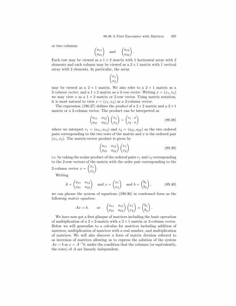
)may be viewed as a 2 × 1 matrix. We also refer to a 2 × 1 matrix as a2-column vector, and a 1× 2 matrix as a 2-row vector. Writing x = (x1, x2)we may view x as a 1 × 2 matrix or 2-row vector. Using matrix notation,it is most natural to view x = (x1, x2) as a 2-column vector.The expression (190.37) defines the product of a 2× 2 matrix and a 2× 1
matrix or a 2-column vector. The product can be interpreted as(a11 a12a21 a22
)(x1
x2
)=
(c1 · xc2 · x
)(89.38)
where we interpret r1 = (a11, a12) and r2 = (a21, a22) as the two orderedpairs corresponding to the two rows of the matrix and x is the ordered pair(x1, x2). The matrix-vector product is given by(
a11 a12a21 a22
)(x1
x2
)(89.39)
i.e. by taking the scalar product of the ordered pairs r1 and r2 correspondingto the 2-row vectors of the matrix with the order pair corresponding to the
2-column vector x =
(x1
x2
).
Writing
A =
(a11 a12a21 a22
)and x =
(x1
x2
)and b =
(b1b2
), (89.40)
we can phrase the system of equations (190.36) in condensed form as thefollowing matrix equation:
Ax = b, or
(a11 a12a21 a22
)(x1
x2
)=
(b1b2
).
We have now got a first glimpse of matrices including the basic operationof multiplication of a 2× 2-matrix with a 2× 1 matrix or 2-column vector.Below we will generalize to a calculus for matrices including addition ofmatrices, multiplication of matrices with a real number, and multiplicationof matrices. We will also discover a form of matrix division referred toas inversion of matrices allowing us to express the solution of the systemAx = b as x = A−1b, under the condition that the columns (or equivalently,the rows) of A are linearly independent.
396 89. Analytic Geometry in R2
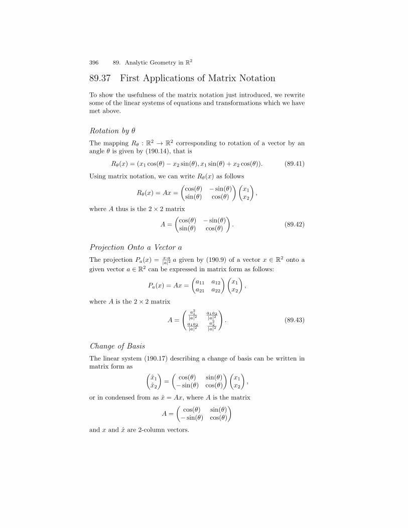
89.37 First Applications of Matrix Notation
To show the usefulness of the matrix notation just introduced, we rewritesome of the linear systems of equations and transformations which we havemet above.
Rotation by θ
The mapping Rθ : R2 → R2 corresponding to rotation of a vector by anangle θ is given by (190.14), that is
Rθ(x) = (x1 cos(θ)− x2 sin(θ), x1 sin(θ) + x2 cos(θ)). (89.41)
Using matrix notation, we can write Rθ(x) as follows
Rθ(x) = Ax =
(cos(θ) − sin(θ)sin(θ) cos(θ)
)(x1
x2
),
where A thus is the 2× 2 matrix
A =
(cos(θ) − sin(θ)sin(θ) cos(θ)
). (89.42)
Projection Onto a Vector a
The projection Pa(x) =x·a|a|2 a given by (190.9) of a vector x ∈ R2 onto a
given vector a ∈ R2 can be expressed in matrix form as follows:
Pa(x) = Ax =
(a11 a12a21 a22
)(x1
x2
),
where A is the 2× 2 matrix
A =
(a21
|a|2a1a2
|a|2a1a2
|a|2a22
|a|2
). (89.43)
Change of Basis
The linear system (190.17) describing a change of basis can be written inmatrix form as (
x1
x2
)=
(cos(θ) sin(θ)− sin(θ) cos(θ)
)(x1
x2
),
or in condensed from as x = Ax, where A is the matrix
A =
(cos(θ) sin(θ)− sin(θ) cos(θ)
)and x and x are 2-column vectors.
89.38 Addition of Matrices 397
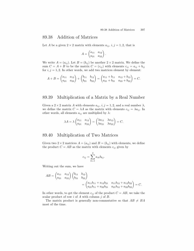
89.38 Addition of Matrices
Let A be a given 2× 2 matrix with elements aij , i, j = 1, 2, that is
A =
(a11 a12a21 a22
).
We write A = (aij). Let B = (bij) be another 2× 2 matrix. We define thesum C = A + B to be the matrix C = (cij) with elements cij = aij + bijfor i, j = 1, 2. In other words, we add two matrices element by element:
A+B =
(a11 a12a21 a22
)+
(b11 b12b21 b22
)=
(a11 + b11 a12 + b12a21 + b21 a22 + b22
)= C.
89.39 Multiplication of a Matrix by a Real Number
Given a 2× 2 matrix A with elements aij , i, j = 1, 2, and a real number λ,we define the matrix C = λA as the matrix with elements cij = λaij . Inother words, all elements aij are multiplied by λ:
λA = λ
(a11 a12a21 a22
)=
(λa11 λa12λa21 λa22
)= C.
89.40 Multiplication of Two Matrices
Given two 2× 2 matrices A = (aij) and B = (bij) with elements, we definethe product C = AB as the matrix with elements cij given by
cij =2∑
k=1
aikbkj .
Writing out the sum, we have
AB =
(a11 a12a21 a22
)(b11 b12b21 b22
)=
(a11b11 + a12b21 a11b12 + a12b22a21b11 + a22b21 a21b12 + a22b22
)= C.
In other words, to get the element cij of the product C = AB, we take thescalar product of row i of A with column j of B.The matrix product is generally non-commutative so that AB = BA
most of the time.
398 89. Analytic Geometry in R2
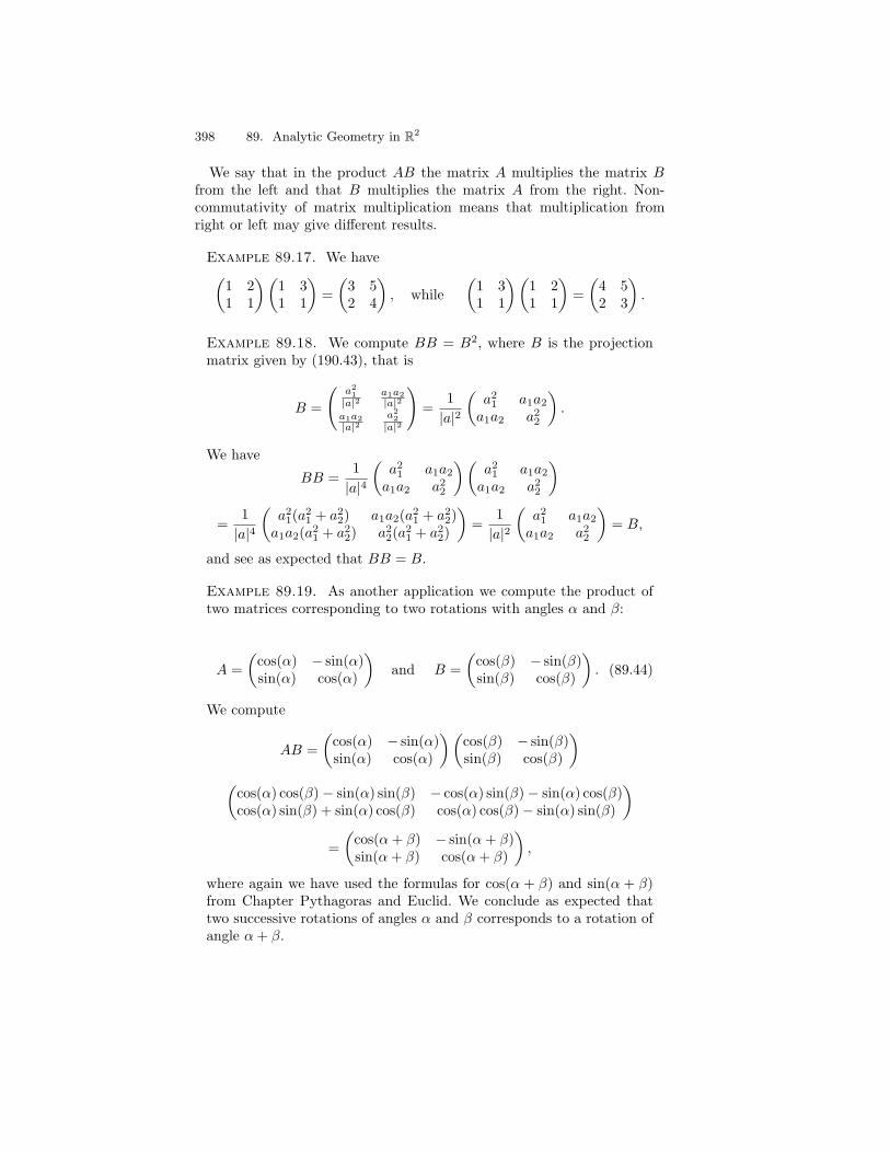
We say that in the product AB the matrix A multiplies the matrix Bfrom the left and that B multiplies the matrix A from the right. Non-commutativity of matrix multiplication means that multiplication fromright or left may give different results.
Example 89.17. We have(1 21 1
)(1 31 1
)=
(3 52 4
), while
(1 31 1
)(1 21 1
)=
(4 52 3
).
Example 89.18. We compute BB = B2, where B is the projectionmatrix given by (190.43), that is
B =
(a21
|a|2a1a2
|a|2a1a2
|a|2a22
|a|2
)=
1
|a|2
(a21 a1a2a1a2 a22
).
We have
BB =1
|a|4
(a21 a1a2a1a2 a22
)(a21 a1a2a1a2 a22
)=
1
|a|4
(a21(a
21 + a22) a1a2(a
21 + a22)
a1a2(a21 + a22) a22(a
21 + a22)
)=
1
|a|2
(a21 a1a2a1a2 a22
)= B,
and see as expected that BB = B.
Example 89.19. As another application we compute the product oftwo matrices corresponding to two rotations with angles α and β:
A =
(cos(α) − sin(α)sin(α) cos(α)
)and B =
(cos(β) − sin(β)sin(β) cos(β)
). (89.44)
We compute
AB =
(cos(α) − sin(α)sin(α) cos(α)
)(cos(β) − sin(β)sin(β) cos(β)
)(cos(α) cos(β)− sin(α) sin(β) − cos(α) sin(β)− sin(α) cos(β)cos(α) sin(β) + sin(α) cos(β) cos(α) cos(β)− sin(α) sin(β)
)=
(cos(α+ β) − sin(α+ β)sin(α+ β) cos(α+ β)
),
where again we have used the formulas for cos(α + β) and sin(α + β)from Chapter Pythagoras and Euclid. We conclude as expected thattwo successive rotations of angles α and β corresponds to a rotation ofangle α+ β.

89.41 The Transpose of a Matrix 399
89.41 The Transpose of a Matrix
Given a 2 × 2 matrix A with elements aij , we define the transpose of Adenoted by A⊤ as the matrix C = A⊤ with elements c11 = a11, c12 = a21,c21 = a12, c22 = a22. In other words, the rows of A are the columns of A⊤
and vice versa. For example
if A =
(1 23 4
)then A⊤ =
(1 32 4
).
Of course (A⊤)⊤ = A. Transposing twice brings back the original matrix.We can directly check the validity of the following rules for computing withthe transpose:
(A+B)⊤ = A⊤ +B⊤, (λA)⊤ = λA⊤,
(AB)⊤ = B⊤A⊤.
89.42 The Transpose of a 2-Column Vector
The transpose of a 2-column vector is the row vector with the same ele-ments:
if x =
(x1
x2
), then x⊤ =
(x1 x2
).
We may define the product of a 1×2 matrix (2-row vector) x⊤ with a 2×1matrix (2-column vector) y in the natural way as follows:
x⊤y =(x1 x2
)(y1y2
)= x1y1 + x2y2.
In particular, we may write
|x|2 = x · x = x⊤x,
where we interpret x as an ordered pair and as a 2-column vector.
89.43 The Identity Matrix
The 2× 2 matrix (1 00 1
)is called the identity matrix and is denoted by I. We have IA = A andAI = A for any 2× 2 matrix A.
400 89. Analytic Geometry in R2
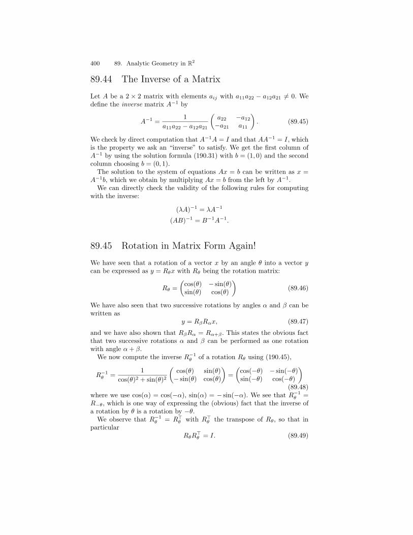
89.44 The Inverse of a Matrix
Let A be a 2 × 2 matrix with elements aij with a11a22 − a12a21 = 0. Wedefine the inverse matrix A−1 by
A−1 =1
a11a22 − a12a21
(a22 −a12−a21 a11
). (89.45)
We check by direct computation that A−1A = I and that AA−1 = I, whichis the property we ask an “inverse” to satisfy. We get the first column ofA−1 by using the solution formula (190.31) with b = (1, 0) and the secondcolumn choosing b = (0, 1).The solution to the system of equations Ax = b can be written as x =
A−1b, which we obtain by multiplying Ax = b from the left by A−1.We can directly check the validity of the following rules for computing
with the inverse:
(λA)−1 = λA−1
(AB)−1 = B−1A−1.
89.45 Rotation in Matrix Form Again!
We have seen that a rotation of a vector x by an angle θ into a vector ycan be expressed as y = Rθx with Rθ being the rotation matrix:
Rθ =
(cos(θ) − sin(θ)sin(θ) cos(θ)
)(89.46)
We have also seen that two successive rotations by angles α and β can bewritten as
y = RβRαx, (89.47)
and we have also shown that RβRα = Rα+β . This states the obvious factthat two successive rotations α and β can be performed as one rotationwith angle α+ β.We now compute the inverse R−1
θ of a rotation Rθ using (190.45),
R−1θ =
1
cos(θ)2 + sin(θ)2
(cos(θ) sin(θ)− sin(θ) cos(θ)
)=
(cos(−θ) − sin(−θ)sin(−θ) cos(−θ)
)(89.48)
where we use cos(α) = cos(−α), sin(α) = − sin(−α). We see that R−1θ =
R−θ, which is one way of expressing the (obvious) fact that the inverse ofa rotation by θ is a rotation by −θ.We observe that R−1
θ = R⊤θ with R⊤
θ the transpose of Rθ, so that inparticular
RθR⊤θ = I. (89.49)

89.46 A Mirror in Matrix Form 401
We use this fact to prove that the length of a vector is not changed byrotation. If y = Rθx, then
|y|2 = yT y = (Rθx)⊤(Rθx) = x⊤R⊤
θ Rθx = x⊤x = |x|2. (89.50)
More generally, the scalar product is preserved after the rotation. If y =Rθx and y = Rθx, then
y · y = (Rθx)⊤(Rθx) = x⊤R⊤
θ Rθx = x · x. (89.51)
The relation (190.49) says that the matrix Rθ is orthogonal. Orthogonalmatrices play an important role, and we will return to this topic below.
89.46 A Mirror in Matrix Form
Consider the linear transformation 2P − I, where Px = a·x|a|2 a is the projec-
tion onto the non-zero vector a ∈ R2, that is onto the line x = sa throughthe origin. In matrix form, this can be expressed as
2P − I =2
|a|2
(a21 − 1 a1a2a2a1 a22 − 1
).
After some reflection(!), looking at Fig. 190.28, we understand that thetransformation I+2(P − I) = 2P − I maps a point x into its mirror imagein the line through the origin with direction a.
a
x Px−x
FIGURE 89.27. The mapping 2P − I maps points to its mirror point relative tothe given line.
To see if 2P −I preserves scalar products, we assume that y = (2P −I)xand y = (2P − I)x and compute:
y · y = ((2P − I)x)⊤(2P − I)x = x⊤(2P⊤ − I)(2P − I)x = (89.52)
x⊤(4P⊤P − 2P⊤I − 2PI + I)x = x⊤(4P − 4P + I)x = x · x, (89.53)

402 89. Analytic Geometry in R2
where we used the fact that P = P⊤ and PP = P , and we thus find anaffirmative answer.
89.47 Change of Basis Again!
Let a1, a2 and a1, a2 be two different bases in R2. We then express anygiven b ∈ R2 as
b = x1a1 + x2a2 = x1a1 + x2a2, (89.54)
with certain coordinates (x1, x2) with respect to a1, a2 and some othercoordinates (x1, x2) with respect a1, a2.To connect (x1, x2) to (x1, x2), we express the basis vectors a1, a2 in
terms of the basis a1, a2:
c11a1 + c21a2 = a1,
c12a1 + c22a2 = a2,
with certain coefficients cij . Inserting this into (190.54), we get
x1(c11a1 + c21a2) + x2(c12a1 + c22a2) = b.
Reordering terms,
(c11x1 + c12x2)a1 + (c21x1 + c22x2)a2 = b.
We conclude by uniqueness that
x1 = c11x1 + c12x2, (89.55)
x2 = c21x1 + c22x2, (89.56)
which gives the connection between the coordinates (x1, x2) and (x1, x2).Using matrix notation, we can write this relation as x = Cx with
C =
(c11 c12c21 c22
).
89.48 Queen Christina
Queen Christina of Sweden (1626-1689), daughter of Gustaf Vasa King ofSweden 1611-1632, crowned to Queen at the age 5, officially coronated 1644,abdicated 1652, converted to Catholicism and moved to Rome 1655.Throughout her life, Christina had a passion for the arts and for learning,
and surrounded herself with musicians, writers, artists and also philoso-phers, theologians, scientists and mathematicians. Christina had an im-pressive collection of sculpture and paintings, and was highly respected for

89.48 Queen Christina 403
/PSfrag wherepop(x1)[[0(Bl)1 0]](x2)[[1(Bl)1 0]](b)[[2(Bl)1 0]](a1)[[3(Bl)1 0]](a2)[[4(Bl)1 0]](b1)[[5(Bl)1 0]](b2)[[6(Bl)1 0]](hatb1)[[7(Bl)1 0]](hatb2)[[8(Bl)1 0]](hata1)[[9(Bl)1 0]](hata2)[[10(Bl)1 0]]11 0 1/Begin PSfraguserdict /PSfragpopputifelse
b
b2
b2x1
x2
hata1
hatb1hatb1
b
a1
a2
hata2
/End PSfrag /Hide PSfragPSfrag replacements/Unhide PSfrag– x1 0/Place PSfrag– x2 1/Place PSfrag– b 2/Place PSfrag– a1 3/Place PSfrag– a2 4/Place PSfrag– b1 5/Place PSfrag– b2 6/Place PSfrag– b1 7/Place PSfrag– b2 8/Place PSfrag– a1 9/Place PSfrag– a2 10/Place PSfrag
FIGURE 89.28. A vector b may be expressed in terms of the basis a1, a2 or thebasis a1, a2.
both her artistic and literary tastes. She also wrote several books, includ-ing her Letters to Descartes and Maxims. Her home, the Palace Farnese,was the active center of cultural and intellectual life in Rome for severaldecades.Duc de Guise quoted in Georgina Masson’s Queen Christina biography
describes Queen Chistina as follows: “She isn’t tall, but has a well-filledfigure and a large behind, beautiful arms, white hands. One shoulder ishigher than another, but she hides this defect so well by her bizarre dress,walk and movements.... The shape of her face is fair but framed by themost extraordinary coiffure. It’s a man’s wig, very heavy and piled highin front, hanging thick at the sides, and at the back there is some slightresemblance to a woman’s coiffure.... She is always very heavily powderedover a lot of face cream”.
Chapter 89 Problems
89.1. Given the vectors a, b and c in R2 and the scalars λ, µ ∈ R, prove thefollowing statements
a+ b = b+ a, (a+ b) + c = a+ (b+ c), a+ (−a) = 0
a+ 0 = a, 3a = a+ a+ a, λ(µa) = (λµ)a,
(λ+ µ)a = λa+ µa, λ(a+ b) = λa+ λb, |λa| = |λ||a|.Try to give both analytical and geometrical proofs.
89.2. Give a formula for the transformation f : R2 → R2 corresponding toreflection through the direction of a given vector a ∈ R2. Find the correspondingmatrix.
89.3. Given a = (3, 2) and b = (1, 4), compute (i) |a|, (ii) |b|, (iii) |a + b|, (iv))|a− b|, (v) a/|a|, (vi) b/|b|.

404 89. Analytic Geometry in R2
FIGURE 89.29. Queen Christina to Descartes: “If we conceive the world in thatvast extension you give it, it is impossible that man conserve himself thereinin this honorable rank, on the contrary, he shall consider himself along withthe entire earth he inhabits as in but a small, tiny and in no proportion tothe enormous size of the rest. He will very likely judge that these stars haveinhabitants, or even that the earths surrounding them are all filled with creaturesmore intelligent and better than he, certainly, he will lose the opinion that thisinfinite extent of the world is made for him or can serve him in any way”.
89.48 Queen Christina 405
89.4. Show that the norm of a/|a| with a ∈ R2, a = 0, is equal to 1.
89.5. Given a, b ∈ R2 prove the following inequalities a) |a + b| ≤ |a| + |b|, b)a · b ≤ |a||b|.
89.6. Compute a · b with
(i) a = (1, 2), b = (3, 2) (ii) a = (10, 27), b = (14,−5)
89.7. Given a, b, c ∈ R2, determine which of the following statements make sense:(i) a · b, (ii) a · (b · c), (iii) (a · b) + |c|, (iv) (a · b) + c, (v) |a · b|.
89.8. What is the angle between a = (1, 1) and b = (3, 7)?
89.9. Given b = (2, 1) construct the set of all vectors a ∈ R2 such that a · b = 2.Give a geometrical interpretation of this result.
89.10. Find the projection of a onto b onto (1, 2) with (i) a = (1, 2), (ii) a =(−2, 1), (iii) a = (2, 2), (iv) a = (
√2,√2).
89.11. Decompose the vector b = (3, 5) into one component parallel to a andone component orthogonal to a for all vectors a in the previous exercise.
89.12. Let a, b and c = a− b in R2 be given, and let the angle between a and bbe φ. Show that:
|c|2 = |a|2 + |b|2 − 2|a||b| cosφ.Give an interpretation of the result.
89.13. Prove the law of cosines for a triangle with sidelengths a, b and c:
c2 = a2 + b2 − 2ab cos(θ),
where θ is the angle between the sides a and b.
89.14. Given the 2 by 2 matrix:
A =
(1 23 4
)compute Ax and ATx for the following choice of x ∈ R2:
(i) xT = (1, 2) (ii) xT = (1, 1)
89.15. Given the 2× 2-matrices:
A =
(1 23 4
), B =
(5 67 8
),
compute (i) AB, (ii) BA, (iii) ATB, (iv) ABT , (v) BTAT , (vi) (AB)T , (vii) A−1,(viii) B−1, (ix) (AB)−1, (x) A−1A.
89.16. Show that (AB)T = BTAT and that (Ax)T = xTAT .

406 89. Analytic Geometry in R2
89.17. What can be said about A if: a) A = AT b) AB = I?
89.18. Show that the projection:
Pa(b) =b · a|a|2 a
can be written in the form Pb, where P is a 2 × 2 matrix. Show that PP = Pand P = PT .
89.19. Compute the mirror image of a point with respect to a straight line inR2 which does not pass through the origin. Express the mapping in matrix form.
89.20. Express the linear transformation of rotating a vector a certain givenangle as a matrix vector product.
89.21. Given a, b ∈ R2, show that the “mirror vector” b obtained by reflectingb in a can be expressed as:
b = 2Pb− b
where P is a certain projection Show that the scalar product between two vectorsis invariant under a reflection, that is
c · d = c · d.
89.22. Compute a× b and b× a with (i) a = (1, 2), b = (3, 2), (ii) a = (1, 2), b =(3, 6), (iii) a = (2,−1), b = (2, 4).
89.23. Extend the Matlab functions for vectors in R2 by writing functions forvector product (x = vecProd(a, b)) and rotation (b = vecRotate(a, angle)) ofvectors.
89.24. Check the answers to the above problems using Matlab.
89.25. Verify that the projection Px = Pa(x) is linear in x. Is it linear also ina? Illustrate, as in Fig. 190.17, that Pa(x+ y) = Pa(x) + Pa(y).
89.26. Prove that the formula (191.29) for the projection of a point onto a linethrough the origin, coincides with the formula (190.9) for the projection of thevector b on the direction of the line.
89.27. Show that if a = λa, where a is a nonzero vector R2 and λ = 0, thenfor any b ∈ R2 we have Pa(b) = Pa(b), where Pa(b) is the projection of b onto a.Conclude that the projection onto a non-zero vector a ∈ R2 only depends on thedirection of a and not the norm of a.

This is page 407Printer: Opaque this
90Analytic Geometry in R3
We must confess that in all humility that, while number is a productof our mind alone, space has a reality beyond the mind whose ruleswe cannot completely prescribe. (Gauss 1830)
You can’t help respecting anybody who can spell TUESDAY, evenif he doesn’t spell it right. (The House at Pooh Corner, Milne)
90.1 Introduction
We now extend the discussion of analytic geometry to Euclidean three di-mensional space or Euclidean 3d space for short. We imagine this spacearises when we draw a normal through the origin to a Euclidean two di-mensional plane spanned by orthogonal x1 and x2 axes, and call the normalthe x3-axis. We then obtain an orthogonal coordinate system consisting ofthree coordinate x1, x2 and x3 axes that intersect at the origin, with eachaxis being a copy of R, see Fig. 191.1.In daily life, we may imagine a room where we live as a portion of R3,
with the horizontal floor being a piece of R2 with two coordinates (x1, x2)and with the vertical direction as the third coordinate x3. On a largerscale, we may imagine our neighborhood in terms of three orthogonal di-rections West-East, South-North, and Down-Up, which may be viewed tobe a portion of R3, if we neglect the curvature of the Earth.The coordinate system can be oriented two ways, right or left. The coor-
dinate system is said to be right-oriented, which is the standard, if turning
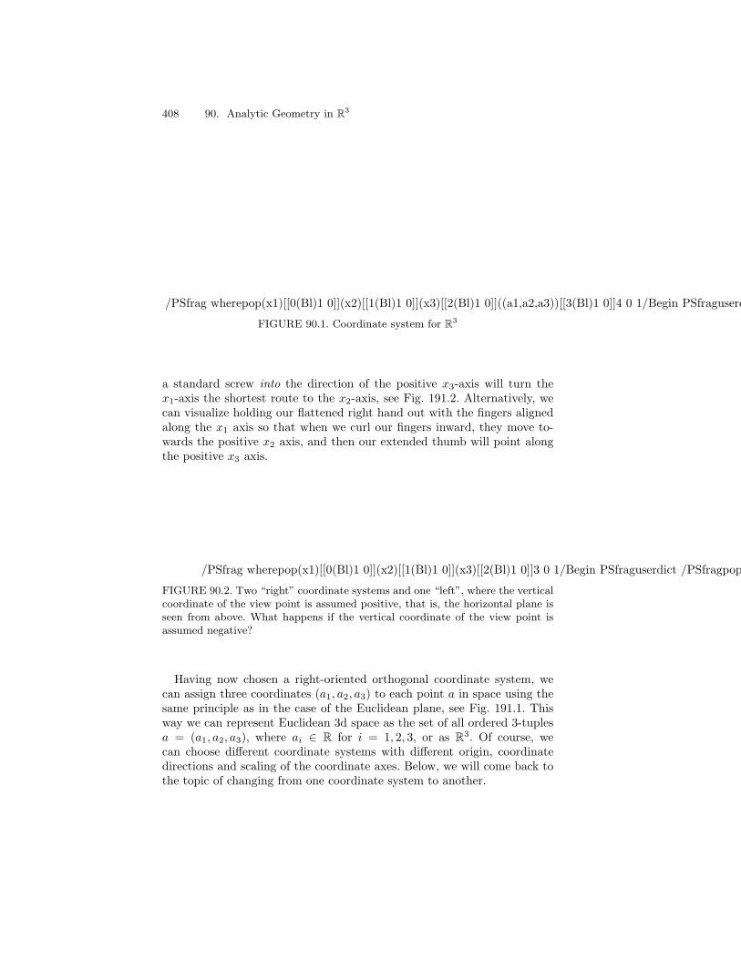
408 90. Analytic Geometry in R3
/PSfrag wherepop(x1)[[0(Bl)1 0]](x2)[[1(Bl)1 0]](x3)[[2(Bl)1 0]]((a1,a2,a3))[[3(Bl)1 0]]4 0 1/Begin PSfraguserdict /PSfragpopputifelsex1
x2
x3 x3
x1
(a1,a2,a3)
(a1,a2,a3)
x2
/End PSfrag /Hide PSfragPSfrag replacements/Unhide PSfrag– x1 0/Place PSfrag– x2 1/Place PSfrag– x3 2/Place PSfrag– (a1, a2, a3)˝ 3/Place PSfrag
FIGURE 90.1. Coordinate system for R3
a standard screw into the direction of the positive x3-axis will turn thex1-axis the shortest route to the x2-axis, see Fig. 191.2. Alternatively, wecan visualize holding our flattened right hand out with the fingers alignedalong the x1 axis so that when we curl our fingers inward, they move to-wards the positive x2 axis, and then our extended thumb will point alongthe positive x3 axis.
/PSfrag wherepop(x1)[[0(Bl)1 0]](x2)[[1(Bl)1 0]](x3)[[2(Bl)1 0]]3 0 1/Begin PSfraguserdict /PSfragpopputifelsex1
x2
x3
x3
x1
x2
x1
x3
x2
/End PSfrag /Hide PSfragPSfrag replacements/Unhide PSfrag– x1 0/Place PSfrag– x2 1/Place PSfrag– x3 2/Place PSfrag
FIGURE 90.2. Two “right” coordinate systems and one “left”, where the verticalcoordinate of the view point is assumed positive, that is, the horizontal plane isseen from above. What happens if the vertical coordinate of the view point isassumed negative?
Having now chosen a right-oriented orthogonal coordinate system, wecan assign three coordinates (a1, a2, a3) to each point a in space using thesame principle as in the case of the Euclidean plane, see Fig. 191.1. Thisway we can represent Euclidean 3d space as the set of all ordered 3-tuplesa = (a1, a2, a3), where ai ∈ R for i = 1, 2, 3, or as R3. Of course, wecan choose different coordinate systems with different origin, coordinatedirections and scaling of the coordinate axes. Below, we will come back tothe topic of changing from one coordinate system to another.

90.2 Vector Addition and Multiplication by a Scalar 409
90.2 Vector Addition and Multiplication by aScalar
Most of the notions and concepts of analytic geometry of the Euclideanplane represented by R2 extend naturally to Euclidean 3d space representedby R3.In particular, we can view an ordered 3-tuple a = (a1, a2, a3) either as
a point in three dimensional space with coordinates a1, a2 and a3 or as avector/arrow with tail at the origin and head at the point (a1, a2, a3), asillustrated in Fig. 191.1.We define the sum a+b of two vectors a = (a1, a2, a3) and b = (b1, b2, b3)
in R3 by componentwise addition,
a+ b = (a1 + b1, a2 + b2, a3 + b3),
and multiplication of a vector a = (a1, a2, a3) by a real number λ by
λa = (λa1, λa2, λa3).
The zero vector is the vector 0 = (0, 0, 0). We also write −a = (−1)a anda − b = a + (−1)b. The geometric interpretation of these definitions isanalogous to that in R2. For example, two non-zero vectors a and b in R3
are parallel if b = λa for some non-zero real number λ. The usual ruleshold, so vector addition is commutative, a + b = b + a, and associative,(a + b) + c = a + (b + c). Further, λ(a + b) = λa + λb and κ(λa) = (κλ)afor vectors a and b and real numbers λ and κ.The standard basis vectors in R3 are e1 = (1, 0, 0), e2 = (0, 1, 0) and
e3 = (0, 0, 1).
90.3 Scalar Product and Norm
The standard scalar product a · b of two vectors a = (a1, a2, a3) and b =(b1, b2, b3) in R3 is defined by
a · b =3∑
i=1
aibi = a1b1 + a2b2 + a3b3. (90.1)
The scalar product in R3 has the same properties as its cousin in R2, so itis bilinear, symmetric, and positive definite.= We say that two vectors aand b are orthogonal if a · b = 0.The Euclidean length or norm |a| of a vector a = (a1, a2, a3) is defined
by
|a| = (a · a) 12 =
( 3∑i=1
a2i) 1
2 , (90.2)
410 90. Analytic Geometry in R3
which expresses Pythagoras theorem in 3d, and which we may obtain byusing the usual 2d Pythagoras theorem twice. The distance |a− b| betweentwo points a = (a1, a2, a3) and b = (b1, b2, b3) is equal to
|a− b| =( 3∑i=1
(ai − bi)2)1/2
.
Cauchy’s inequality states that for any vectors a and b in R3,
|a · b| ≤ |a| |b|. (90.3)
We give a proof of Cauchy’s inequality in Chapter Analytic Geometry inRn below. We note that Cauchy’s inequality in R2 follows directly from thefact that a · b = |a| |b| cos(θ), where θ is the angle between a and b.
90.4 Projection of a Vector onto a Vector
Let a be a given non-zero vector in R3. We define the projection Pb = Pa(b)of a vector b in R3 onto the vector a by the formula
Pb = Pa(b) =a · ba · a
a =a · b|a|2
a. (90.4)
This is a direct generalization of the corresponding formula in R2 basedon the principles that Pb is parallel to a and b − Pb is orthogonal to a asillustrated in Fig. 191.3, that is
Pb = λa for some λ ∈ R and (b− Pb) · a = 0.
This gives the formula (191.4) with λ = a·b|a|2 .
The transformation P : R3 → R3 is linear, that is for any b and c ∈ R3
and λ ∈ R,P (b+ c) = Pb+ Pc, P (λb) = λPb,
and PP = P .
90.5 The Angle Between Two Vectors
We define the angle θ between non-zero vectors a and b in R3 by
cos(θ) =a · b|a| |b|
, (90.5)

90.6 Vector Product 411
where we may assume that 0 ≤ θ ≤ 180. By Cauchy’s inequality (191.3),|a · b| ≤ |a| |b|. Thus, there is an angle θ satisfying (191.5) that is uniquelydefined if we require 0 ≤ θ ≤ 180. We may write (191.5) in the form
a · b = |a||b| cos(θ), (90.6)
where θ is the angle between a and b. This evidently extends the corre-sponding result in R2.We define the angle θ between two vectors a and b via the scalar product
a · b in (191.5), which we may view as an algebraic definition. Of course,we would like to see that this definition coincides with a usual geometricdefinition. If a and b both lie in the x1 − x2-plane, then we know fromthe Chapter Analytic geometry in R2 that the two definitions coincide. Weshall see below that the scalar product a · b is invariant (does not change)under rotation of the coordinate system, which means that given any twovectors a and b, we can rotate the coordinate system so make a and b liein the x1 − x2-plane. We conclude that the algebraic definition (191.5) ofangle between two vectors and the usual geometric definition coincide. Inparticular, two non-zero vectors are geometrically orthogonal in the sensethat the geometric angle θ between the vectors satisfies cos(θ) = 0 if andonly if a · b = |a||b| cos(θ) = 0.
/PSfrag wherepop(x1)[[0(Bl)1 0]](x2)[[1(Bl)1 0]](x3)[[2(Bl)1 0]](a)[[3(Bl)1 0]](b)[[4(Bl)1 0]](Pb)[[5(Bl)1 0]](theta)[[6(Bl)1 0]]7 0 1/Begin PSfraguserdict /PSfragpopputifelse
bb
theta
x1
x2
x3
x1
x2
x3
thetaPb
a a
Pb
/End PSfrag /Hide PSfragPSfrag replacements/Unhide PSfrag– x1 0/Place PSfrag– x2 1/Place PSfrag– x3 2/Place PSfrag– a 3/Place PSfrag– b 4/Place PSfrag– P b5/Place PSfrag– θ 6/Place PSfrag
FIGURE 90.3. Projection Pb of a vector b onto a vector a.
90.6 Vector Product
We now define the vector product a× b of two vectors a = (a1, a2, a3) andb = (b1, b2, b3) in R3 by the formula
a× b = (a2b3 − a3b2, a3b1 − a1b3, a1b2 − a2b1). (90.7)

412 90. Analytic Geometry in R3
We note that the vector product a× b of two vectors a and b in R3 is itselfa vector in R3. In other words, with f(a, b) = a× b, f : R3 → R3. We alsorefer to the vector product as the cross product, because of the notation.
Example 90.1. If a = (3, 2, 1) and b = (4, 5, 6), then a × b = (12 −5, 4− 18, 15− 8) = (7,−14, 7).
Note that there is also the trivial, componentwise “vector product” de-fined by (using MATLAB c⃝ ’s notation) a.∗b = (a1b1, a2b2, a3b3). The vectorproduct defined above, however, is something quite different!The formula for the vector product may seem a bit strange (and com-
plicated), and we shall now see how it arises. We start by noting that theexpression a1b2 − a2b1 appearing in (191.7) is the vector product of thevectors (a1, a2) and (b1, b2) in R2, so there appears to be some pattern atleast.We may directly check that the vector product a× b is linear in both a
and b, that is
a× (b+ c) = a× b+ a× c, (a+ b)× c = a× c+ b× c, (90.8a)
(λa)× b = λ a× b, a× (λb) = λa× b, (90.8b)
where the products × should be computed first unless something else isindicated by parentheses. This follows directly from the fact that the com-ponents of a× b depend linearly on the components of a and b.Since the vector product a× b is linear in both a and b, we say that a× b
is bilinear. We also see that the vector product a × b is anti-symmetric inthe sense that
a× b = − b× a. (90.9)
Thus, the vector product a× b is bilinear and antisymmetric and moreoverit turns out that these two properties determine the vector product up toa constant just as in in R2.For the vector products of the basis vectors ei, we have (check this!)
ei × ei = 0, i = 1, 2, 3, (90.10a)
e1 × e2 = e3, e2 × e3 = e1, e3 × e1 = e2, (90.10b)
e2 × e1 = −e3, e3 × e2 = −e1, e1 × e3 = −e2. (90.10c)
We see that e1×e2 = e3 is orthogonal to both e1 and e2. Similarly, e2×e3 =e1 is orthogonal to both e2 and e3, and e1×e3 = −e2 is orthogonal to bothe1 and e3.This pattern generalizes. In fact, for any two non-zero vectors a and b,
the vector a× b is orthogonal to both a and b since
a ·(a×b) = a1(a2b3−a3b2)+a2(a3b1−a1b3)+a3(a1b2−a2b1) = 0, (90.11)
90.7 Geometric Interpretation of the Vector Product 413
and similarly b · (a× b) = 0.We may compute the vector product of two arbitrary vectors a = (a1, a2,
a3) and b = (b1, b2, b3) by using linearity combined with (191.10) as follows,
a× b = (a1e1 + a2e2 + a3e3)× (b1e1 + b2e2 + b3e3)
= a1b2 e1 × e2 + a2b1 e2 × e1
+ a1b3 e1 × e3 + a3b1 e3 × e1
+ a2b3 e2 × e3 + a3b2 e3 × e2
= (a1b2 − a2b1)e3 + (a3b1 − a1b3)e2 + (a2b3 − a3b2)e1
= (a2b3 − a3b2, a3b1 − a1b3, a1b2 − a2b1),
which conforms with (191.7).
90.7 Geometric Interpretation of the VectorProduct
We shall now make a geometric interpretation of the vector product a× bof two vectors a and b in R3.We start by assuming that a = (a1, a2, 0) and b = (b1, b2, 0) are two
non-zero vectors in the plane defined by the x1 and x2 axes. The vectora×b = (0, 0, a1b2−a2b1) is clearly orthogonal to both a and b, and recallingthe basic result (190.21) for the vector product in R2, we have
|a× b| = |a||b|| sin(θ)|, (90.12)
where θ is the angle between a and b.We shall now prove that this result generalizes to arbitrary vectors a =
(a1, a2, a3) and b = (b1, b2, b3) in R3. First, the fact that a× b is orthogonalto both a and b was proved in the previous section. Secondly, we note thatmultiplying the trigonometric identity sin2(θ) = 1− cos2(θ) by |a|2 |b|2 andusing (191.6), we obtain
|a|2|b|2 sin2(θ) = |a|2|b|2 − (a · b)2. (90.13)
Finally, a direct (but somewhat lengthy) computation shows that
|a× b|2 = |a|2|b|2 − (a · b)2,
which proves (191.12). We summarize in the following theorem.
Theorem 90.1 The vector product a× b of two non-zero vectors a and bin R3 is orthogonal to both a and b and |a × b| = |a||b|| sin(θ)|, where θ isthe angle between a and b. In particular, a and b are parallel if and only ifa× b = 0.
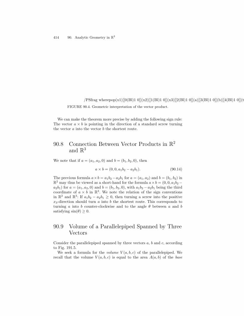
414 90. Analytic Geometry in R3
/PSfrag wherepop(x1)[[0(Bl)1 0]](x2)[[1(Bl)1 0]](x3)[[2(Bl)1 0]](a)[[3(Bl)1 0]](b)[[4(Bl)1 0]](theta)[[5(Bl)1 0]](axb)[[6(Bl)1 0]](—axb—=A(a,b)=—a——b——sin(theta)—)[[7(Bl)1 0]]8 0 1/Begin PSfraguserdict /PSfragpopputifelse
b
axb
|axb|=A(a,b)=|a||b||sin(theta)|
x1
x3
atheta
x2
/End PSfrag /Hide PSfragPSfrag replacements/Unhide PSfrag– x1 0/Place PSfrag– x2 1/Place PSfrag– x3 2/Place PSfrag– a 3/Place PSfrag– b 4/Place PSfrag– θ 5/Place PSfrag– a×b˝ 6/Place PSfrag– |a×b| = A(a, b) = |a| |b| | sin(θ)|˝ 7/Place PSfrag
FIGURE 90.4. Geometric interpretation of the vector product.
We can make the theorem more precise by adding the following sign rule:The vector a × b is pointing in the direction of a standard screw turningthe vector a into the vector b the shortest route.
90.8 Connection Between Vector Products in R2
and R3
We note that if a = (a1, a2, 0) and b = (b1, b2, 0), then
a× b = (0, 0, a1b2 − a2b1). (90.14)
The previous formula a×b = a1b2−a2b1 for a = (a1, a2) and b = (b1, b2) inR2 may thus be viewed as a short-hand for the formula a×b = (0, 0, a1b2−a2b1) for a = (a1, a2, 0) and b = (b1, b2, 0), with a1b2− a2b1 being the thirdcoordinate of a × b in R3. We note the relation of the sign conventionsin R2 and R3: If a1b2 − a2b1 ≥ 0, then turning a screw into the positivex3-direction should turn a into b the shortest route. This corresponds toturning a into b counter-clockwise and to the angle θ between a and bsatisfying sin(θ) ≥ 0.
90.9 Volume of a Parallelepiped Spanned by ThreeVectors
Consider the parallelepiped spanned by three vectors a, b and c, accordingto Fig. 191.5.We seek a formula for the volume V (a, b, c) of the parallelepiped. We
recall that the volume V (a, b, c) is equal to the area A(a, b) of the base
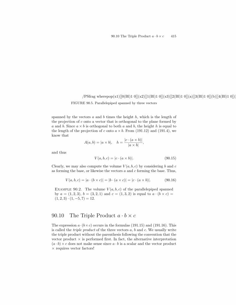
90.10 The Triple Product a · b× c 415
/PSfrag wherepop(x1)[[0(Bl)1 0]](x2)[[1(Bl)1 0]](x3)[[2(Bl)1 0]](a)[[3(Bl)1 0]](b)[[4(Bl)1 0]](c)[[5(Bl)1 0]](theta)[[6(Bl)1 0]](axb)[[7(Bl)1 0]]8 0 1/Begin PSfraguserdict /PSfragpopputifelse
b
axb
c
x1
x2
x3
thetaa
/End PSfrag /Hide PSfragPSfrag replacements/Unhide PSfrag– x1 0/Place PSfrag– x2 1/Place PSfrag– x3 2/Place PSfrag– a 3/Place PSfrag– b 4/Place PSfrag– c 5/Place PSfrag– θ 6/Place PSfrag– a×b˝ 7/Place PSfrag
FIGURE 90.5. Parallelepiped spanned by three vectors
spanned by the vectors a and b times the height h, which is the length ofthe projection of c onto a vector that is orthogonal to the plane formed bya and b. Since a× b is orthogonal to both a and b, the height h is equal tothe length of the projection of c onto a× b. From (191.12) and (191.4), weknow that
A(a, b) = |a× b|, h =|c · (a× b)||a× b|
,
and thus
V (a, b, c) = |c · (a× b)|. (90.15)
Clearly, we may also compute the volume V (a, b, c) by considering b and cas forming the base, or likewise the vectors a and c forming the base. Thus,
V (a, b, c) = |a · (b× c)| = |b · (a× c)| = |c · (a× b)|. (90.16)
Example 90.2. The volume V (a, b, c) of the parallelepiped spannedby a = (1, 2, 3), b = (3, 2, 1) and c = (1, 3, 2) is equal to a · (b × c) =(1, 2, 3) · (1,−5, 7) = 12.
90.10 The Triple Product a · b× c
The expression a · (b×c) occurs in the formulas (191.15) and (191.16). Thisis called the triple product of the three vectors a, b and c. We usually writethe triple product without the parenthesis following the convention that thevector product × is performed first. In fact, the alternative interpretation(a · b)× c does not make sense since a · b is a scalar and the vector product× requires vector factors!

416 90. Analytic Geometry in R3
The following properties of the triple product can be readily verified bydirect application of the definition of the scalar and vector products,
a · b× c = c · a× b = b · c× a,
a · b× c = −a · c× b = −b · a× c = −c · b× a.
To remember these formulas, we note that if two of the vectors change placethen the sign changes, while if all three vectors are cyclically permuted (forexample the order a, b, c is replaced by c, a, b or b, c, a), then the sign isunchanged.Using the triple product a · b× c, we can express the geometric quantity
of the volume V (a, b, c) of the parallelepiped spanned by a, b and c in theconcise algebraic form,
V (a, b, c) = |a · b× c|. (90.17)
We shall use this formula many times below. Note, we later prove that thevolume of a parallelepiped can be computed as the area of the base timesthe height using Calculus below.
90.11 A Formula for the Volume Spanned byThree Vectors
Let a1 = (a11, a12, a13), a2 = (a21, a22, a23) and a3 = (a31, a32, a33) be threevectors in R3. Note that here a1 is a vector in R3 with a1 = (a11, a12, a13),et cetera. We may think of forming the 3 × 3 matrix A = (aij) with therows corresponding to the coordinates of a1, a2 and a3,
A =
a11 a12 a13a21 a22 a23a31 a32 a33
We will come back to 3 × 3 matrices below. Here, we just use the matrixto express the coordinates of the vectors a1, a2 and a3 in handy form.We give an explicit formula for the volume V (a1, a2, a3) spanned by three
vectors a1, a2 and a3. By direct computation starting with (191.17),
±V (a1, a2, a3) = a1 · a2 × a3
= a11(a22a33 − a23a32)− a12(a21a33 − a23a31)
+ a13(a21a32 − a22a31).
(90.18)
We note that V (a1, a2, a3) is a sum of terms, each term consisting of theproduct of three factors aijaklamn with certain indices ij, kl and mn. If weexamine the indices occurring in each term, we see that the sequence of row

90.12 Lines 417
indices ikm (first indices) is always 1, 2, 3, while the sequence of columnindices jln (second indices) corresponds to a permutation of the sequence1, 2, 3, that is the numbers 1, 2 and 3 occur in some order. Thus, allterms have the form
a1j1a2j2a3j3 (90.19)
with j1, j2, j3 being a permutation of 1, 2, 3. The sign of the termschange with the permutation. By inspection we can detect the followingpattern: if the permutation can be brought to the order 1, 2, 3 with aneven number of transpositions, each transposition consisting of interchang-ing two indices, then the sign is +, and with an uneven number of transpo-sitions the sign is −. For example, the permutation of second indices in theterm a11a23a32 is 1, 3, 2, which is uneven since one transposition brings itback to 1, 2, 3, and thus this term has a negative sign. Another example:the permutation in the term a12a23a31 is 2, 3, 1 is even since it resultsfrom the following two transpositions 2, 1, 3 and 1, 2, 3.We have now developed a technique for computing volumes that we will
generalize to Rn below. This will lead to determinants. We will see thatthe formula (191.18) states that the signed volume ±V (a1, a2, a3) is equalto the determinant of the 3× 3 matrix A = (aij).
90.12 Lines
Let a be a given non-zero vector in R3 and let x be a given point in R3.The points x in R3 of the form
x = x+ sa,
where s varies over R, form a line in R3 through the point x with directiona, see Fig. 191.6. If x = 0, then the line passes through the origin.
Example 90.3. The line through (1, 2, 3) in the direction (4, 5, 6) isgiven by
x = (1, 2, 3) + s(4, 5, 6) = (1 + 4s, 2 + 5s, 3 + 6s) s ∈ R.
The line through (1, 2, 3) and (3, 1, 2) has the direction (3, 1, 2)−(1, 2, 3)= (2,−1,−1), and is thus given by x = (1, 2, 3) + s(2,−1,−1).
Note that by choosing other vectors to represent the direction of theline, it may also be represented, for example, as x = (1, 2, 3)+s(−2, 1, 1)or x = (1, 2, 3)+s(6,−3,−3). Also, the “point of departure” on the line,corresponding to s = 0, can be chosen arbitrarily on the line of course.For example, the point (1, 2, 3) could be replaced by (−1, 3, 4) which isanother point on the line.

418 90. Analytic Geometry in R3
/PSfrag wherepop(x1)[[0(Bl)1 0]](x2)[[1(Bl)1 0]](x3)[[2(Bl)1 0]](a)[[3(Bl)1 0]](sa)[[4(Bl)1 0]](hatx)[[5(Bl)1 0]](x=hatx+sa)[[6(Bl)1 0]]7 0 1/Begin PSfraguserdict /PSfragpopputifelse
x1
x2
x3
hatx
a
sa
x=hatx+sa
/End PSfrag /Hide PSfragPSfrag replacements/Unhide PSfrag– x1 0/Place PSfrag– x2 1/Place PSfrag– x3 2/Place PSfrag– a 3/Place PSfrag– s a4/Place PSfrag– x 5/Place PSfrag– x = x+ s a˝ 6/Place PSfrag
FIGURE 90.6. Line in R3 of the form x = x+ s a.
90.13 Projection of a Point onto a Line
Let x = x + sa be a line in R3 through x with direction a ∈ R3. We seekthe projection Pb of a given point b ∈ R3 onto the line, that is we seekPb ∈ R3 with the property that (i) Pb = x + sa for some s ∈ R, and (ii)(b−Pb) ·a = 0. Note that we here view b to be a point rather than a vector.Inserting (i) into (ii) gives the following equation in s: (b− x− sa) · a = 0,from which we conclude that s = b·a−x·a
|a|2 , and thus
Pb = x+b · a− x · a
|a|2a . (90.20)
If x = 0, that is the line passes through the origin, then Pb = b·a|a|2 a in
conformity with the corresponding formula (190.9) in R2.
90.14 Planes
Let a1 and a2 be two given non-zero non-parallel vectors in R3, that isa1 × a2 = 0. The points x in R3 that can be expressed as
x = s1a1 + s2a2, (90.21)
where s1 and s2 vary over R, form a plane in R3 through the origin thatis spanned by the two vectors a1 and a2. The points x in the plane areall the linear combinations x = s1a1 + s2a2 of the vectors a1 and a2 withcoefficients s1 and s2 varying over R, see Fig. 191.7. The vector a1 × a2 isorthogonal to both a1 and a2 and therefore to all vectors x in the plane.Thus, the non-zero vector n = a1× a2 is a normal to the plane. The pointsx in the plane are characterized by the orthogonality relation
n · x = 0. (90.22)
90.14 Planes 419
We may thus describe the points x in the plane by the representation(191.21) or the equation (191.22). Note that (191.21) is a vector equationcorresponding to 3 scalar equations, while (191.22) is a scalar equation.Eliminating the parameters s1 and s2 in the system (191.21), we obtainthe scalar equation (191.22).Let x be a given point in R3. The points x in R3 that can be expressed
asx = x+ s1a1 + s2a2, (90.23)
where s1 and s2 vary over R, form a plane in R3 through the point x thatis parallel to the corresponding plane through the origin considered above,see Fig. 191.8.If x = x+s1a1+s2a2 then n ·x = n · x, because n ·ai = 0, i = 1, 2. Thus,
we can describe the points x of the form x = x+ s1a1 + s2a2 alternativelyas the vectors x satisfying
n · x = n · x. (90.24)
Again, we obtain the scalar equation (191.24) if we eliminate the parameterss1 and s2 in the system (191.23).We summarize:
Theorem 90.2 A plane in R3 through a point x ∈ R3 with normal ncan be expressed as the set of x ∈ R3 of the form x = x + s1a1 + s2a2with s1 and s2 varying over R, where a1 and a2 are two vectors satisfyingn = a1 × a2 = 0. Alternatively, the plane can be described as the set ofx ∈ R such that n · x = d, where d = n · x.
Example 90.4. Consider the plane x1 + 2x2 + 3x3 = 4, that is theplane (1, 2, 3) · (x1, x2, x3) = 4 with normal n = (1, 2, 3). To write thepoints x in this plane on the form x = x+s1a1+s2a2, we first choose apoint x in the plane, for example, x = (2, 1, 0) noting that n · x = 4. Wenext choose two non-parallel vectors a1 and a2 such that n · a1 = 0 andn·a2 = 0, for example a1 = (−2, 1, 0) and a2 = (−3, 0, 1). Alternatively,we choose one vector a1 satisfying n ·a1 = 0 and set a2 = n×a1, whichis a vector orthogonal to both n and a1. To find a vector a1 satisfyinga1 ·n = 0, we may choose an arbitrary non-zero vector m non-parallel ton and set a1 = m× n, for example m = (0, 0, 1) giving a1 = (−2, 1, 0).
Conversely, given the plane x = (2, 1, 0) + s1(−2, 1, 0) + s2(−3, 0, 1),that is x = x + s1a1 + s2a2 with x = (2, 1, 0), a1 = (−2, 1, 0) anda2 = (−3, 0, 1), we obtain the equation x1 + 2x2 + 3x3 = 4 simply bycomputing n = a1 × a2 = (1, 2, 3) and n · x = (1, 2, 3) · (2, 1, 0) = 4,from which we obtain the following equation for the plane: n · x =(1, 2, 3) · (x1, x2, x3) = x1 + 2x2 + 3x3 = n · x = 4.
Example 90.5. Consider the real-valued function z = f(x, y) = ax+by+ c of two real variables x and y, where a, b and c are real numbers.

420 90. Analytic Geometry in R3
/PSfrag wherepop(x1)[[0(Bl)1 0]](x2)[[1(Bl)1 0]](x3)[[2(Bl)1 0]](a1)[[3(Bl)1 0]](a2)[[4(Bl)1 0]](n=a1xa2)[[5(Bl)1 0]](x=s1a1+s2a2)[[6(Bl)1 0]]7 0 1/Begin PSfraguserdict /PSfragpopputifelse
x=s1a1+s2a2
x1
x2
x3
a1
a2
n=a1xa2
/End PSfrag /Hide PSfragPSfrag replacements/Unhide PSfrag– x1 0/Place PSfrag– x2 1/Place PSfrag– x3 2/Place PSfrag– a1 3/Place PSfrag– a2 4/Place PSfrag– n = a1×a2˝ 5/Place PSfrag– x = s1a1 + s2a2˝ 6/Place PSfrag
FIGURE 90.7. Plane through the origin spanned by a1 and a2, and with normaln = a1 × a2.
/PSfrag wherepop(x1)[[0(Bl)1 0]](x2)[[1(Bl)1 0]](x3)[[2(Bl)1 0]](a1)[[3(Bl)1 0]](a2)[[4(Bl)1 0]](n=a1xa2)[[5(Bl)1 0]](x=s1a1+s2a2)[[6(Bl)1 0]](hatx)[[7(Bl)1 0]](x=hatx+s1a1+s2a2)[[8(Bl)1 0]]9 0 1/Begin PSfraguserdict /PSfragpopputifelse
x=hatx+s1a1+s2a2hatx
x=s1a1+s2a2x1
x2
x3
a1
a2
n=a1xa2
/End PSfrag /Hide PSfragPSfrag replacements/Unhide PSfrag– x1 0/Place PSfrag– x2 1/Place PSfrag– x3 2/Place PSfrag– a1 3/Place PSfrag– a2 4/Place PSfrag– n = a1×a2˝ 5/Place PSfrag– x = s1a1 + s2a2˝ 6/Place PSfrag– x 7/Place PSfrag– x = x+ s1a1 + s2a2˝ 8/Place PSfrag
FIGURE 90.8. Plane through x with normal n defined by n · x = d = n · x.

90.15 The Intersection of a Line and a Plane 421
Setting x1 = x, x2 = y and x3 = z, we can express the graph ofz = f(x, y) as the plane ax1 + bx2 − x3 = −c in R3 with normal(a, b,−1).
90.15 The Intersection of a Line and a Plane
We seek the intersection of a line x = x+sa and a plane n·x = d that is theset of points x belonging to both the line and the plane, where x, a, n andd are given. Inserting x = x+ sa into n · x = d, we obtain n · (x+ sa) = d,that is n · x+ s n · a = d. This yields s = (d− n · x)/(n · a) if n · a = 0, andwe find a unique point of intersection
x = x+ (d− n · x)/(n · a) a. (90.25)
This formula has no meaning if n · a = 0, that is if the line is parallel tothe plane. In this case, there is no intersection point unless x happens tobe a point in the plane and then the whole line is part of the plane.
Example 90.6. The intersection of the plane x1 + 2x2 + x3 = 5and the line x = (1, 0, 0) + s(1, 1, 1) is found by solving the equation1 + s + 2s + s = 5 giving s = 1 and thus the point of intersection is(2, 1, 1).The plane x1+2x2+x3 = 5 and the line x = (1, 0, 0)+s(2,−1, 0)has no point of intersection, because the equation 1 + 2s− 2s = 5 hasno solution. If instead we consider the plane x1 +2x2 + x3 = 1, we findthat the entire line x = (1, 0, 0) + s(2,−1, 0) lies in the plane, because1 + 2s− 2s = 1 for all real s.
90.16 Two Intersecting Planes Determine a Line
Let n1 = (n11, n12, n13) and n2 = (n21, n22, n23) be two vectors in R3 andd1 and d2 two real numbers. The set of points x ∈ R3 that lie in both theplane n1 · x = d1 and n2 · x = d2 satisfy the system of two equations
n1 · x = d1,
n2 · x = d2.(90.26)
Intuition indicates that generally the points of intersection of the two planesshould form a line in R3. Can we determine the formula of this line in theform x = x+ sa with suitable vectors a and x in R3 and s varying over R?Assuming first that d1 = d2 = 0, we seek a formula for the set of x suchthat n1 · x = 0 and n2 · x = 0, that is the set of x that are orthogonal toboth n1 and n2. This leads to a = n1 × n2 and expressing the solution xof the equations n1 · x = 0 and n2 · x = 0 as x = s n1 × n2 with s ∈ R. Of

422 90. Analytic Geometry in R3
course it is natural to add in the assumption that n1 ×n2 = 0, that is thatthe two normals n1 and n2 are not parallel so that the two planes are notparallel.Next, suppose that (d1, d2) = (0, 0). We see that if we can find one vector
x such that n1 · x = d1 and n2 · x = d2, then we can write the solution x of(191.26) as
x = x+ s n1 × n2, s ∈ R. (90.27)
We now need to verify that we can indeed find x satisfying n1 · x = d1 andn2 · x = d2. That is, we need to find x ∈ R3 satisfying the following systemof two equations,
n11x1 + n12x2 + n13x3 = d1,
n21x1 + n22x2 + n23x3 = d2.
Since n1 × n2 = 0, some component of n1 × n2 must be nonzero. If forexample n11n22 − n12n21 = 0, corresponding to the third component ofn1 × n2 being non-zero, then we may choose x3 = 0. Then recalling therole of the condition n11n22 − n12n21 = 0 for a 2 × 2-system, we maysolve uniquely for x1 and x2 in terms of d1 and d2 to get a desired x. Theargument is similar in case the second or first component of n1×n2 happensto be non-zero.We summarize:
Theorem 90.3 Two non-parallel planes n1 · x = d1 and n2 · x = d2 withnormals n1 and n2 satisfying n1 × n2 = 0, intersect along a straight linewith direction n1 × n2.
Example 90.7. The intersection of the two planes x1+x2+x3 = 2 and3x1+2x2−x3 = 1 is given by x = x+sa with a = (1, 1, 1)×(3, 2,−1) =(−3, 4,−1) and x = (0, 1, 1).
90.17 Projection of a Point onto a Plane
Let n · x = d be a plane in R3 with normal n and b a point in R3. We seekthe projection Pb of b onto the plane n · x = d. It is natural to ask Pb tosatisfy the following two conditions, see Fig. 191.9,
n · Pb = d, that is Pb is a point in the plane,
b− Pb is parallel to the normal n, that is b− Pb = λn for some λ ∈ R.
We conclude that Pb = b − λn and the equation n · Pb = d thus givesn · (b− λn) = d. So, λ = b·n−d
|n|2 and thus
Pb = b− b · n− d
|n|2n. (90.28)

90.18 Distance from a Point to a Plane 423
If d = 0 so the plane n · x = d = 0 passes through the origin, then
Pb = b− b · n|n|2
n. (90.29)
If the plane is given in the form x = x+ s1a1 + s2a2 with a1 and a2 twogiven non-parallel vectors in R3, then we may alternatively compute theprojection Pb of a point b onto the plane by seeking real numbers x1 andx2 so that Pb = x+ x1a1 + x2a2 and (b−Pb) · a1 = (b−Pb) · a2 = 0. Thisgives the system of equations
x1a1 · a1 + x2a2 · a1 = b · a1 − x · a1,x1a1 · a2 + x2a2 · a2 = b · a2 − x · a2
(90.30)
in the two unknowns x1 and x2. To see that this system has a uniquesolution, we need to verify that a11a22 − a12a21 = 0, where a11 = a1 · a1,a22 = a2 ·a2, a21 = a2 ·a1 and a12 = a1 ·a2. This follows from the fact thata1 and a2 are non-parallel, see Problem 191.24.
Example 90.8. The projection Pb of the point b = (2, 2, 3) ontothe plane defined by x1 + x2 + x3 = 1 is given by Pb = (2, 2, 3) −7−13 (1, 1, 1) = (0, 0, 1).
Example 90.9. The projection Pb of the point b = (2, 2, 3) onto theplane x = (1, 0, 0) + s1(1, 1, 1) + s2(1, 2, 3) with normal n = (1, 1, 1) ×(1, 2, 3) = (1,−2, 1) is given by Pb = (2, 2, 3)− (2,2,3)·(1,−2,1)
6 (1,−2, 1) =(2, 2, 3)− 1
6 (1,−2, 1) = 16 (11, 14, 17).
90.18 Distance from a Point to a Plane
We say that the distance from a point b to a plane n · x = d is equal to|b − Pb|, where Pb is the projection of b onto the plane. According to theprevious section, we have
|b− Pb| = |b · n− d||n|
.
Note that this distance is equal to the shortest distance between b and anypoint in the plane, see Fig. 191.9 and Problem 191.22.
Example 90.10. The distance from the point (2, 2, 3) to the plane
x1 + x2 + x3 = 1 is equal to |(2,2,3)·(1,1,1)−1|√3
= 2√3.

424 90. Analytic Geometry in R3
/PSfrag wherepop(x1)[[0(Bl)1 0]](x2)[[1(Bl)1 0]](x3)[[2(Bl)1 0]](n)[[3(Bl)1 0]](b)[[4(Bl)1 0]](Pb)[[5(Bl)1 0]](b-Pb)[[6(Bl)1 0]]7 0 1/Begin PSfraguserdict /PSfragpopputifelse
b
x2
x3
n
Pb
x1
b−Pb
/End PSfrag /Hide PSfragPSfrag replacements/Unhide PSfrag– x1 0/Place PSfrag– x2 1/Place PSfrag– x3 2/Place PSfrag– n 3/Place PSfrag– b 4/Place PSfrag– P b5/Place PSfrag– b−Pb˝ 6/Place PSfrag
FIGURE 90.9. Projection of a point/vector onto a plane.
90.19 Rotation Around a Given Vector
We now consider a more difficult problem. Let a ∈ R3 be a given vectorand θ ∈ R a given angle. We seek the transformation R : R3 → R3 corre-sponding to rotation of an angle θ around the vector a. Recalling Section190.21, the result Rx = R(x) should satisfy the following properties,
(i) |Rx−Px| = |x−Px|, (ii) (Rx−Px) · (x−Px) = cos(θ)|x−Px|2.
where Px = Pa(x) is the projection of x onto a, see Fig. 191.10. We write
/PSfrag wherepop(x1)[[0(Bl)1 0]](x2)[[1(Bl)1 0]](x3)[[2(Bl)1 0]](x)[[3(Bl)1 0]](Px)[[4(Bl)1 0]](Rx)[[5(Bl)1 0]](theta)[[6(Bl)1 0]]7 0 1/Begin PSfraguserdict /PSfragpopputifelse
xRx
Px
x1
x2
x3
theta
/End PSfrag /Hide PSfragPSfrag replacements/Unhide PSfrag– x1 0/Place PSfrag– x2 1/Place PSfrag– x3 2/Place PSfrag– x 3/Place PSfrag– P x4/Place PSfrag– Rx5/Place PSfrag– θ 6/Place PSfrag
FIGURE 90.10. Rotation around a = (0, 0, 1) a given angle θ.
Rx−Px as Rx−Px = α(x−Px)+β a× (x−Px) for real numbers α andβ, noting that Rx− Px is orthogonal to a and a× (x− Px) is orthogonalto both a and (x− Px). Taking the scalar product with (x− Px), we use
(ii) to get α = cos(θ) and then use (i) to find β = sin(θ)|a| with a suitable

90.20 Lines and Planes Through the Origin Are Subspaces 425
orientation. Thus, we may express Rx in terms of the projection Px as
Rx = Px+ cos(θ)(x− Px) +sin(θ)
|a|a× (x− Px). (90.31)
90.20 Lines and Planes Through the Origin AreSubspaces
Lines and planes in R3 through the origin are examples of subspaces of R3.The characteristic feature of a subspace is that the operations of vectoraddition and scalar multiplication does not lead outside the subspace. Forexample if x and y are two vectors in the plane through the origin withnormal n satisfying n · x = 0 and n · y = 0, then n · (x + y) = 0 andn · (λx) = 0 for any λ ∈ R, so the vectors x+ y and λx also belong to theplane. On the other hand, if x and y belong to a plane not passing throughthe origin with normal n, so that n · x = d and n · y = d with d a nonzeroconstant, then n · (x+y) = 2d = d, and thus x+y does not lie in the plane.We conclude that lines and planes through the origin are subspaces of R3,but lines and planes not passing through the origin are not subspaces. Theconcept of subspace is very basic and we will meet this concept many timesbelow.We note that the equation n · x = 0 defines a line in R2 and a plane
in R3. The equation n · x = 0 imposes a constraint on x that reduces thedimension by one, so in R2 we get a line and in R3 we get a plane.
90.21 Systems of 3 Linear Equations in 3Unknowns
Consider now the following system of 3 linear equations in 3 unknowns x1,x2 and x3 (as did Leibniz already 1683):
a11x1 + a12x2 + a13x3 = b1,a21x1 + a22x2 + a23x3 = b2,a31x1 + a32x2 + a33x3 = b3,
(90.32)
with coefficients aij and right hand side bi, i, j = 1, 2, 3. We can write thissystem as the following vector equation in R3:
x1a1 + x2a2 + x3a3 = b, (90.33)
where a1 = (a11, a21, a31), a2 = (a12, a22, a32), a3 = (a13, a23, a33) andb = (b1, b2, b3) are vectors in R3, representing the given coefficients and theright hand side.

426 90. Analytic Geometry in R3
When is the system (191.32) uniquely solvable in x = (x1, x2, x3) for agiven right hand side b? We shall see that the condition to guarantee uniquesolvability is
V (a1, a2, a3) = |a1 · a2 × a3| = 0, (90.34)
stating that the volume spanned by a1, a2 and a3 is not zero.We now argue that the condition a1 ·a2×a3 = 0 is the right condition to
guarantee the unique solvability of (191.32). We can do this by mimickingwhat we did in the case of a 2×2 system: Taking the scalar product of bothsides of the vector equation x1a1+x2a2+x3a3 = b by successively a2×a3,a3 × a1, and a2 × a3, we get the following solution formula (recalling thata1 · a2 × a3 = a2 · a3 × a1 = a3 · a1 × a2):
x1 =b · a2 × a3a1 · a2 × a3
,
x2 =b · a3 × a1a2 · a3 × a1
=a1 · b× a3a1 · a2 × a3
,
x3 =b · a1 × a2a3 · a1 × a2
=a1 · a2 × b
a1 · a2 × a3,
(90.35)
where we used the facts that ai · aj × ak = 0 if any two of the indices i,j and k are equal. The solution formula (191.35) shows that the system(191.32) has a unique solution if a1 · a2 × a3 = 0.Note the pattern of the solution formula (191.35), involving the common
denominator a1 · a2 × a3 and the numerator for xi is obtained by replacingai by b. The solution formula (191.35) is also called Cramer’s rule. We haveproved the following basic result:
Theorem 90.4 If a1 · a2 × a3 = 0, then the system of equations (191.32)or the equivalent vector-equation (191.33) has a unique solution given byCramer’s rule (191.35).
We repeat: V (a1, a2, a3) = a1 · a2 × a3 = 0 means that the three vectorsa1, a2 and a3 span a non-zero volume and thus point in three differentdirections (such that the plane spanned by any two of the vectors does notcontain the third vector). If V (a1, a2, a3) = 0, then we say that the set ofthree vectors a,a2, a3 is linearly independent, or that the three vectorsa1, a2 and a3 are linearly independent.
90.22 Solving a 3× 3-System by GaussianElimination
We now describe an alternative to Cramer’s rule for computing the solutionto the 3 × 3-system of equations (191.32), using the famous method ofGaussian elimination. Assuming a11 = 0, we subtract the first equation

90.22 Solving a 3× 3-System by Gaussian Elimination 427
multiplied by a21 from the second equation multiplied by a11, and likewisesubtract the first equation multiplied by by a31 from the third equationmultiplied by a11, to rewrite the system (191.32) in the form
a11x1 + a12x2 + a13x3 = b1,(a22a11 − a21a12)x2 + (a23a11 − a21a13)x3 = a11b2 − a21b1,(a32a11 − a31a12)x2 + (a33a11 − a31a13)x3 = a11b3 − a31b1,
(90.36)where the unknown x1 has been eliminiated in the second and third equa-tions. This system has the form
a11x1+ a12x2 + a13x3 = b1,
a22x2 + a23x3 = b2,
a32x2 + a33x3 = b3,
(90.37)
with modified coefficients aij and bi. We now proceed in the same wayconsidering the 2× 2-system in (x2, x3), and bring the system to the finaltriangular form
a11x1+ a12x2 + a13x3 = b1,
a22x2 + a23x3 = b2,
a33x3 = b3,
(90.38)
with modified coefficients in the last equation. We can now solve the thirdequation for x3, then insert the resulting value of x3 into the second equa-tion and solve for x2 and finally insert x3 and x2 into the first equation tosolve for x1.
Example 90.11. We give an example of Gaussian elimination: Con-sider the system
x1 +2x2 + 3x3 = 6,2x1 +3x2 + 4x3 = 9,3x1 +4x2 + 6x3 = 13.
Subtracting the first equation multiplied by 2 from the second and thefirst equation multiplied by 3 from the third equation, we get the system
x1 +2x2 + 3x3 = 6,−x2 − 2x3 = −3,−2x2 − 3x3 = −5.
Subtracting now the second equation multiplied by 2 from the thirdequation, we get
x1 + 2x2+ 3x3 = 6,−x2− 2x3 = −3,
x3 = 1,
from which we find x3 = 1 and then from the second equation x2 = 1and finally from the first equation x1 = 1.

428 90. Analytic Geometry in R3
90.23 3× 3 Matrices: Sum, Product and Transpose
We can directly generalize the notion of a 2× 2 matrix as follows: We saythat the quadratic array a11 a12 a13
a21 a22 a23a31 a32 a33
is a 3×3 matrix A = (aij) with elements aij , i, j = 1, 2, 3, and with i beingthe row index and j the column index.Of course, we can also generalize the notion of a 2-row (or 1× 2 matrix)
and a 2-column vector (or 2×1 matrix). Each row of A, the first row being(a11 a12 a13), can thus be viewed as a 3-row vector (or 1× 3 matrix), andeach column of A, the first column beinga11
a21a31
as a 3-column vector (or 3 × 1 matrix). We can thus view a 3 × 3 matrixto consist of three 3-row vectors or three 3-column vectors.Let A = (aij) and B = (bij) be two 3 × 3 matrices. We define the sum
C = A + B to be the matrix C = (cij) with elements cij = aij + bij fori, j = 1, 2, 3. In other words, we add two matrices element by element.Given a 3 × 3 matrix A = (aij) and a real number λ, we define the
matrix C = λA as the matrix with elements cij = λaij . In other words, allelements aij are multiplied by λ.Given two 3× 3 matrices A = (aij) and B = (bij), we define the product
C = AB as the 3× 3 matrix with elements cij given by
cij =3∑
k=1
aikbkj i, j = 1, 2, 3. (90.39)
Matrix multiplication is associative so that (AB)C = A(BC) for matricesA, B and C, see Problem 191.10. The matrix product is however not com-mutative in general, that is there are matrices A and B such that AB = BA,see Problem 191.11.Given a 3× 3 matrix A = (aij), we define the transpose of A denoted by
A⊤ as the matrix C = A⊤ with elements cij = aji, i, j = 1, 2, 3. In otherwords, the rows of A are the columns of A⊤ and vice versa. By definition(A⊤)⊤ = A. Transposing twice brings back the original matrix.We can directly check the validity of the following rules for computing
with the transpose:
(A+B)⊤ = A⊤ +B⊤, (λA)⊤ = λA⊤,
(AB)⊤ = B⊤A⊤.

90.23 3× 3 Matrices: Sum, Product and Transpose 429
Similarly, the transpose of a 3-column vector is the 3-row vector with thesame elements. Vice versa, if we consider the 3× 1 matrix
x =
x1
x2
x3
to be a 3-column vector, then the transpose x⊤ is the corresponding 3-rowvector (x1 x2 x3). We define the product of a 1 × 3 matrix (3-row vector)x⊤ with a 3× 1 matrix (3-column vector) y in the natural way as follows:
x⊤y =(x1 x2 x3
)y1y2y3
= x1y1 + x2y2 + x3y3 = x · y,
where we noted the connection to the scalar product of 3-vectors. We thusmake the fundamental observation that multiplication of a 1 × 3 matrix(3-row vector) with a 3× 1 matrix (3-column vector) is the same as scalarmultiplication of the corresponding 3-vectors. We can then express theelement cij of the product C = AB according to (191.39) as the scalarproduct of row i of A with column j of B,
cij =(ai1 ai2 ai3
)b1jb2jb3j
=3∑
k=1
aikbkj .
We note that|x|2 = x · x = x⊤x,
where we interpret x both as an ordered triple and as a 3-column vector.The 3× 3 matrix 1 0 0
0 1 00 0 1
is called the 3 × 3 identity matrix and is denoted by I. We have IA = Aand AI = A for any 3× 3 matrix A.If A = (aij) is a 3×3 matrix and x = (xi) is a 3×1 matrix with elements
xi, then the product Ax is the 3× 1 matrix with elements
3∑k=1
aikxk i = 1, 2, 3.
The linear system of equations
a11x1 + a12x2 + a13x3 = b1,a21x1 + a22x2 + a23x3 = b2,a31x1 + a32x2 + a33x3 = b3,

430 90. Analytic Geometry in R3
can be written in matrix form asa11 a12 a13a21 a22 a23a31 a32 a33
x1
x2
x3
=
b1b2b3
,
that isAx = b,
with A = (aij) and x = (xi) and b = (bi).
90.24 Ways of Viewing a System of LinearEquations
We may view a 3× 3 matrix A = (aij)a11 a12 a13a21 a22 a23a31 a32 a33
as being formed by three column-vectors a1 = (a11, a21, a31), a2 = (a12, a22,a32), a3 = (a13, a23, a33), or by three row-vectors a1 = (a11, a12, a13), a2 =(a21, a22, a23), a3 = (a31, a32, a33). Accordingly, we may view the system ofequations a11 a12 a13
a21 a22 a23a31 a32 a33
x1
x2
x3
=
b1b2b3
,
as a vector equation in the column vectors:
x1a1 + x2a2 + x3a3 = b, (90.40)
or as a system of 3 scalar equations:
a1 · x = b1a2 · x = b2a3 · x = b3,
(90.41)
where the rows ai may be interpreted as normals to planes. We know fromthe discussion following (191.34) that (191.40) can be uniquely solved if±V (a1, a2, a3) = a1 · a2 × a3 = 0.We also know from Theorem 191.3 that if a2 × a3 = 0, then the set
of x ∈ R3 satisfying the two last equations of (191.41) forms a line withdirection a2× a3. If a1 is not orthogonal to a2× a3 then we expect this lineto meet the plane given by the first equation of (191.41) at one point. Thus,if a1 · a2 × a3 = 0 then (191.41) should be uniquely solvable. This leadsto the conjecture that V (a1, a2, a3) = 0 if and only if V (a1, a2, a3) = 0.In fact, direct inspection from the formula (191.18) gives the more preciseresult,

90.25 Non-Singular Matrices 431
Theorem 90.5 If a1, a2 and a3 are the vectors formed by the columns ofa 3× 3 matrix A, and a1, a2 and a3 are the vectors formed by the rows ofA, then V (a1, a2, a3) = V (a1, a2, a3).
90.25 Non-Singular Matrices
Let A be a 3×3 matrix formed by three 3-column vectors a1, a2, and a3. IfV (a1, a2, a3) = 0 then we say that A is non-singular, and if V (a1, a2, a3) = 0then we say that A is singular. From Section 191.21, we know that if A isnon-singular then the matrix equation Ax = b has a unique solution x foreach b ∈ R3. Further, if A is singular then the three vectors a1, a2 and a3lie in the same plane and thus we can express one of the vectors as a linearcombination of the other two. This implies that there is a non-zero vectorx = (x1, x2, x3) such that Ax = 0. We sum up:
Theorem 90.6 If A is a non-singular 3 × 3 matrix then the system ofequations Ax = b is uniquely solvable for any b ∈ R3. If A is singular thenthe system Ax = 0 has a non-zero solution x.
90.26 The Inverse of a Matrix
Let A be a non-singular 3 × 3 matrix. Let ci ∈ R3 be the solution to theequation Aci = ei for i = 1, 2, 3, where the ei denote the standard basisvectors here interpreted as 3-column vectors. Let C = (cij) be the matrixwith columns consisting of the vectors ci. We then have AC = I, where Iis the 3× 3 identity matrix, because Aci = ei. We call C the inverse of Aand write C = A−1 and note that A−1 is a 3× 3 matrix such that
AA−1 = I, (90.42)
that is multiplication of A by A−1 from the right gives the identity. We nowwant to prove that also A−1A = I, that is that we get the identity also bymultiplying A from the left by A−1. To see this, we first note that A−1 mustbe non-singular, since if A−1 was singular then there would exist a non-zerovector x such that A−1x = 0 and multiplying by A from the left would giveAA−1x = 0, contradicting the fact that by (191.42) AA−1x = Ix = x = 0.Multiplying AA−1 = I with A−1 from the left, we get A−1AA−1 = A−1,from which we conclude that A−1A = I by multiplying from the right withthe inverse of A−1, which we know exists since A−1 is non-singular.We note that (A−1)−1 = A, which is a restatement of A−1A = I, and
that(AB)−1 = B−1A−1
since B−1A−1AB = B−1B = I. We summarize:

432 90. Analytic Geometry in R3
Theorem 90.7 If A is a 3× 3 non-singular matrix, then the inverse 3× 3matrix A−1 exists, and AA−1 = A−1A = I. Further, (AB)−1 = B−1A−1.
90.27 Different Bases
Let a1, a2, a3 be a linearly independent set of three vectors in R3, thatis assume that V (a1, a2, a3) = 0. Theorem 191.4 implies that any givenb ∈ R3 can be uniquely expressed as a linear combination of a1, a2, a3,
b = x1a1 + x2a2 + x3a3, (90.43)
or in matrix languageb1b2b3
=
a11 a12 a13a21 a22 a23a31 a32 a33
x1
x2
x3
or b = Ax,
where the columns of the matrix A = (aij) are formed by the vectors a1 =(a11, a21, a31), a2 = (a12, a22, a32), a3 = (a13, a23, a33). Since V (a1, a2, a3) =0, the system of equations Ax = b has a unique solution x ∈ R3 for anygiven b ∈ R3, and thus any b ∈ R3 can be expressed uniquely as a linearcombination b = x1a1 + x2a2 + x3a3 of the set of vectors a1, a2, a3 withthe coefficients (x1, x2, x3). This means that a1, a2, a3 is a basis for R3
and we say that (x1, x2, x3) are the coordinates of b with respect to thebasis a1, a2, a3. The connection between the coordinates (b1, b2, b3) of bin the standard basis and the coordinates x of b in the basis a1, a2, a3 isgiven by Ax = b or x = A−1b.
90.28 Linearly Independent Set of Vectors
We say that a set of three vectors a1, a2, a3 in R3 is linearly independentif V (a1, a2, a3) = 0. We just saw that a linearly independent set a1, a2, a3of three vectors can be used as a basis in R3.If the set a1, a2, a3 is linearly independent then the system Ax = 0 in
which the columns of the 3× 3 matrix are formed by the coefficients of a1,a2 and a3 has no other solution than x = 0.Conversely, as a test of linear dependence we can use the following crite-
rion: if Ax = 0 implies that x = 0, then a1, a2, a3 is linearly independentand thus V (a1, a2, a3) = 0.We summarize:
Theorem 90.8 A set a1, a2, a3 of 3 vectors in R3 is linearly independentand can be used as a basis for R3 if ±V (a1, a2, a3) = a1 ·a2×a3 = 0. A seta1, a2, a3 of 3 vectors in R3 is linearly independent if and only if Ax = 0implies that x = 0.

90.29 Orthogonal Matrices 433
90.29 Orthogonal Matrices
A 3 × 3 matrix Q satisfying Q⊤Q = I is called an orthogonal matrix. Anorthogonal matrix is non-singular with Q−1 = Q⊤ and thus also QQ⊤ = I.An orthogonal matrix is thus characterized by the relation Q⊤Q = QQ⊤ =I.Let qi = (q1i, q2i, q3i) for i = 1, 2, 3, be the column vectors of Q, that is
the row vectors of Q⊤. Stating that Q⊤Q = I is the same as stating that
qi · qj = 0 for i = j, and |qi| = 1,
that is the columns of an orthogonal matrix Q are pairwise orthogonal andhave length one.
Example 90.12. The matrix
Q =
cos(θ) − sin(θ) 0sin(θ) cos(θ) 0
0 0 1
, (90.44)
is orthogonal and corresponds to rotation of an angle θ around the x3
axis.
90.30 Linear Transformations Versus Matrices
Let A = (aij) be a 3×3 matrix. The mapping x → Ax, that is the functiony = f(x) = Ax, is a transformation from R3 to R3. This transformation islinear since A(x+y) = Ax+Ay and A(λx) = λAx for λ ∈ R. Thus, a 3×3matrix A generates a linear transformation f : R3 → R3 with f(x) = Ax.Conversely to each linear transformation f : R3 → R3, we can associate
a matrix A with coefficients given by
aij = fi(ej)
where f(x) = (f1(x), f2(x), f3(x)). The linearity of f(x) implies
f(x) = (f1(3∑
j=1
xjej), f2(3∑
j=1
xjej), f3(3∑
j=1
xjej))⊤
= (3∑
j=1
f1(ej)xj ,3∑
j=1
f2(ej)xj ,3∑
j=1
f3(ej)xj)⊤
= (
3∑j=1
a1jxj ,
3∑j=1
a2jxj ,
3∑j=1
a3jxj)⊤ = Ax,
which shows that a linear transformation f : R3 → R3 can be representedas f(x) = Ax with the matrix A = (aij) with coefficients aij = fi(ej).
434 90. Analytic Geometry in R3
Example 90.13. The projection Px = x·a|a|2 a onto a non-zero vector
a ∈ R3 takes the matrix form
Px =
a21
|a|2a1a2
|a|2a1a3
|a|2a2a1
|a|2a22
|a|2a2a3
|a|2a3a1
|a|2a3a2
|a|2a23
|a|2
x1
x2
x3
Example 90.14. The projection Px = x− x·n
|n|2n onto a plane n ·x = 0
through the origin takes the matrix form
Px =
1− n2
1
|n|2 −n1n2
|n|2 −n1n3
|n|2
−n2n1
|n|2 1− n22
|n|2 −n2n3
|n|2
−n3n1
|n|2 −n3n2
|n|2 1− n23
|n|2
x1
x2
x3
Example 90.15. The mirror image of a point x with respect to a planethrough the origin given by (2P − I)x, where Px is the projection of xonto the plane, takes the matrix form
(2P − I)x =
2
a21
|a|2 − 1 2a1a2
|a|2 2a1a3
|a|2
2a2a1
|a|2 2a22
|a|2 − 1 2a2a3
|a|2
2a3a1
|a|2 2a3a2
|a|2 2a23
|a|2 − 1
x1
x2
x3
90.31 The Scalar Product Is Invariant UnderOrthogonal Transformations
Let Q be the matrix q1, q2, q2 formed by taking the columns to be thebasis vectors qj . We assume that Q is orthogonal, which is the same as as-suming that q1, q2, q2 is an orthogonal basis, that is the qj are pairwise or-thogonal and have length 1. The coordinates x of a vector x in the standardbasis with respect to the basis q1, q2, q2 are given by x = Q−1x = Q⊤x.We shall now prove that if y = Q⊤y, then
x · y = x · y,
which states that the scalar product is invariant under orthogonal coordi-nate changes. We compute
x · y = (Q⊤x) · (Q⊤y) = x · (Q⊤)⊤Q⊤y = x · y,
where we used that for any 3× 3 matrix A = (aij) and x, y ∈ R3
(Ax) · y =
3∑i=1
(
3∑j=1
aijxj)yi =
3∑j=1
(
3∑i=1
aijyi)xj
= (A⊤y) · x = x · (A⊤y),
(90.45)

90.32 Looking Ahead to Functions f : R3 → R3 435
with A = Q⊤, and the facts that (Q⊤)⊤ = Q and QQ⊤ = I.We can now complete the argument about the geometric interpretation
of the scalar product from the beginning of this chapter. Given two non-parallel vectors a and b, we may assume by an orthogonal coordinate trans-formation that a and b belong to the x1 − x2-plane and the geometricinterpretation from Chapter Analytic geometry in R2 carries over.
90.32 Looking Ahead to Functions f : R3 → R3
We have met linear transformations f : R3 → R3 of the form f(x) = Ax,where A is a 3× 3 matrix. Below we shall meet more general (non-linear)transformations f : R3 → R3 that assign a vector f(x) = (f1(x), f2(x),f3(x)) ∈ R3 to each x = (x1, x2, x3) ∈ R3. For example,
f(x) = f(x1, x2, x3) = (x2x3, x21 + x3, x
43 + 5)
with f1(x) = x2x3, f2(x) = x21+x3, f3(x) = x4
3+5. We shall see that we maynaturally extend the concepts of Lipschitz continuity and differentiabilityfor functions f : R → R to functions f : R3 → R3. For example, we saythat f : R3 → R3 is Lipschitz continuous on R3 if there is a constant Lf
such that
|f(x)− f(y)| ≤ Lf |x− y| for all x, y ∈ R3.
Chapter 90 Problems
90.1. Show that the norm |a| of the vector a = (a1, a2, a3) is equal to the distancefrom the origin 0 = (0, 0, 0) to the point (a1, a2, a3). Hint: apply PythagorasTheorem twice.
90.2. Which of the following coordinate systems are righthanded?
/PSfrag wherepop(x1)[[0(Bl)1 0]](x2)[[1(Bl)1 0]](x3)[[2(Bl)1 0]]3 0 1/Begin PSfraguserdict /PSfragpopputifelsex2
x1
x3
x3
x2
x1
x3
x1
x2
/End PSfrag /Hide PSfragPSfrag replacements/Unhide PSfrag– x1 0/Place PSfrag– x2 1/Place PSfrag– x3 2/Place PSfrag
436 90. Analytic Geometry in R3
90.3. Indicate the direction of a × b and b × a in Fig. 191.1 if b points in thedirection of the x1-axis. Consider also the same question in Fig. 191.2.
90.4. Given a = (1, 2, 3) and b = (1, 3, 1), compute a× b.
90.5. Compute the volume of the parallelepiped spanned by the three vectors(1, 0, 0), (1, 1, 1) and (−1,−1, 1).
90.6. What is the area of the triangle formed by the three points: (1, 1, 0),(2, 3,−1) and (0, 5, 1)?
90.7. Given b = (1, 3, 1) and a = (1, 1, 1), compute a) the angle between a andb, b) the projection of b onto a, c) a unit vector orthogonal to both a and b.
90.8. Consider a plane passing through the origin with normal n = (1, 1, 1) anda vector a = (1, 2, 3). Which point p in the plane has the shortest distance to a?
90.9. Is it true or not that for any 3 × 3 matrices A, B, and C and number λ(a) A+B = B +A, (b) (A+B) +C = A+ (B +C), (c) λ(A+B) = λA+ λB?
90.10. Prove that for 3 × 3 matrices A, B and C: (AB)C = A(BC). Hint:Use that D = (AB)C has the elements dij =
∑3k=1(
∑3l=1 ailblk)ckj , and do the
summation in a different order.
90.11. Give examples of 3×3-matrices A and B such that AB = BA. Is it difficultto find such examples, that is, is it exceptional or “normal” that AB = BA.
90.12. Prove Theorem 191.5.
90.13. Write down the three matrices corresponding to rotations around the x1,x2 and x3 axis.
90.14. Find the matrix corresponding to a rotation by the angle θ around agiven vector b in R3.
90.15. Give the matrix corresponding to be mirroring a vector through thex1 − x2-plane.
90.16. Consider a linear transformation that maps two points p1 and p2 in R3
into the points p1, p2, respectively. Show that all points lying on a straight linebetween p1, p2 will be transformed onto a straight line between p1 and p2.
90.17. Consider two straight lines in R3 given by: a + λb and c + µd wherea, b, c, d ∈ R3, λ, µ ∈ R. What is the shortest distance between the two lines?
90.18. Compute the intersection of the two lines given by: (1, 1, 0) + λ(1, 2,−3)and (2, 0,−3) + µ(1, 1,−3). Is it a rule or an exception that such an intersectioncan be found?
90.19. Compute the intersection between two planes passing through the originwith normals n1 = (1, 1, 1), n2 = (2, 3, 1). Compute the intersection of these twoplanes and the x1 − x2 plane.
90.32 Looking Ahead to Functions f : R3 → R3 437
/PSfrag wherepop(x1)[[0(Bl)1 0]](x2)[[1(Bl)1 0]](x3)[[2(Bl)1 0]](r)[[3(Bl)1 0]](a)[[4(Bl)1 0]](n)[[5(Bl)1 0]](b)[[6(Bl)1 0]]7 0 1/Begin PSfraguserdict /PSfragpopputifelse
b
a
r
n
x3
x2
x1/End PSfrag /Hide PSfragPSfrag replacements/Unhide PSfrag– x1 0/Place PSfrag– x2 1/Place PSfrag– x3 2/Place PSfrag– r 3/Place PSfrag– a 4/Place PSfrag– n 5/Place PSfrag– b 6/Place PSfrag
90.20. Prove that (191.42) implies that the inverse of A−1 exists.
90.21. Consider a plane through a point r with normal n. Determine the re-flection in the plane at r of a light ray entering in a direction parallel to a givenvector a.
90.22. Show that the distance between a point b and its projection onto a planen · x = d is equal to the shortest distance between b and any point in the plane.Give both a geometric proof based on Pythagoras’ theorem, and an analyticalproof. Hint: For x in the plane write |b− x|2 = |b− Pb+ (Pb− x)|2 = (b− Pb+(Pb− x), b− Pb+ (Pb− x)) and expand using that (b− Pb, Pb− x) = 0).
90.23. Express (191.31) i matrix form.
90.24. Complete the proof of the claim that (191.30) is uniquely solvable.

438 90. Analytic Geometry in R3
90.34 Gosta Mittag-Leffler
The Swedish mentor of Sonya Kovalevskaya was Gosta Mittag-Leffler (1846-1927), famous Swedish mathematician and founder of the prestigous journalActa Mathematica, see Fig. 191.34. The huge mansion of Mittag-Leffler,beautifully situated in in Djursholm, just outside Stockholm, with an im-pressive library, now houses Institut Mittag-Leffler bringing mathemati-cians from all over the world together for work-shops on different themesof mathematics and its applications. Mittag-Leffler made important con-tributions to the theory of functions of a complex variable, see ChapterAnalytic functions below.
FIGURE 90.11. Gosta Mittag-Leffler, Swedish mathematician and founder ofActa Mathematica: “The mathematician’s best work is art, a high perfect art, asdaring as the most secret dreams of imagination, clear and limpid. Mathematicalgenius and artistic genius touch one another”.

This is page 439Printer: Opaque this
91Complex numbers
The imaginary number is a fine and wonderful recourse of the divinespirit, almost an amphibian between being and not being. (Leibniz)
The composition of vast books is a laborious and impoverishingextravagance. To go on for five hundred pages developing an ideawhose perfect oral exposition is possible in a few minutes! A bettercourse of procedure is to pretend that these books already exist, andthen to offer a resume, a commentary...More reasonable, more inept,more indolent, I have preferred to write notes upon imaginary books.(Borges, 1941)
91.1 Introduction
In this chapter, we introduce the set of complex numbers C. A complexnumber, typically denoted by z, is an ordered pair z = (x, y) of real numbersx and y, where x represents the real part of z and y the imaginary part ofz. We may thus identify C with R2 and we often refer to C as the complexplane. We further identify the set of complex numbers with zero imaginarypart with the set of real numbers and write (x, 0) = x, viewing the realline R as the x-axis in the complex plane C. We may thus view C as anextension of R. Similarly, we identify the set of complex numbers withzero real part with the y-axis, which we also refer to as the set of purelyimaginary numbers. The complex number (0, 1) is given a special namei = (0, 1), and we refer to i as the imaginary unit.

440 91. Complex numbers
/PSfrag wherepop(i=(0,1))[[0(Bl)1 0]](1=(1,0))[[1(Bl)1 0]](z=(x,y))[[2(Bl)1 0]](x=Rez)[[3(Bl)1 0]](y=Imz)[[4(Bl)1 0]]5 0 1/Begin PSfraguserdict /PSfragpopputifelse
x=Rez
y=Imz
z=(x,y)
i=(0,1)
1=(1,0)
/End PSfrag /Hide PSfragPSfrag replacements/Unhide PSfrag– i = (0, 1)˝ 0/Place PSfrag– 1 = (1, 0)˝ 1/Place PSfrag– z = (x, y)˝ 2/Place PSfrag– x = Re z˝ 3/Place PSfrag– y = Im z˝ 4/Place PSfrag
FIGURE 91.1. The complex plane C = R2
The operation of addition in C coincides with the operation of vectoraddition in R2. The new aspect of C is the operation of multiplication ofcomplex numbers, which differs from scalar and vector multiplication inR2.The motivation to introduce complex numbers comes from considering
for example the polynomial equation x2 = −1, which has no root if x isrestricted to be a real number. There is no real number x such that x2 = −1since x2 ≥ 0 for x ∈ R. We shall see that if we allow x to be a complexnumber, the equation x2 = −1 becomes solvable and the two roots arex = ±i. More generally, the Fundamental Theorem of Algebra states thatany polynomial equation with real or complex coefficients has a root in theset of complex numbers. In fact, it follows that a polynomial equation ofdegree n has exactly n roots.Introducing the complex numbers finishes the extension process from nat-
ural numbers over integers and rational numbers to real numbers, wherein each case a new class of polynomial equations could be solved. Furtherextensions beyond complex numbers to for example quarternions consistingof quadruples of real numbers were made in the 19th century by Hamilton,but the initial enthusiasm over these constructs faded since no fully con-vincing applications were found. The complex numbers, on the other hand,have turned out to be very useful.
91.2 Addition and Multiplication
We define the sum (a, b) + (c, d) of two complex numbers (a, b) and (c, d),obtained through the operation of addition denoted by +, as follows:
(a, b) + (c, d) = (a+ c, b+ d), (91.1)
91.3 The Triangle Inequality 441
that is we add the real parts and imaginary parts separately. We see thataddition of two complex numbers corresponds to vector addition of the cor-responding ordered pairs or vectors in R2. Of course, we define subtractionsimilarly: (a, b)− (c, d) = (a− c, b− d).We define the product (a, b)(c, d) of two complex numbers (a, b) and (c, d),
obtained through the operation of multiplication, as follows:
(a, b)(c, d) = (ac− bd, ad+ bc). (91.2)
We can readily check using rules for operating with real numbers that theoperations of addition and multiplication of complex numbers obey thecommutative, associative and distributive rules valid for real numbers.If z = (x, y) is a complex number, we can write
z = (x, y) = (x, 0) + (0, y) = (x, 0) + (0, 1)(y, 0) = x+ iy, (91.3)
referring to the identification of complex numbers of the form (x, 0) with x,(and similarly (y, 0) with y of course) and the notation i = (0, 1) introducedabove. We refer to x is the real part of z and y as the imaginary part of z,writing x = Re z and y = Im z, that is
z = Re z + i Im z = (Re z, Im z). (91.4)
We note in particular that
i2 = i i = (0, 1)(0, 1) = (−1, 0) = −(1, 0) = −1, (91.5)
and thus z = i solves the equation z2 + 1 = 0. Similarly, (−i)2 = −1, andthus the equation z2 + 1 = 0 has the two roots z = ±i.The rule (192.2) for multiplication of two complex numbers (a, b) and
(c, d), can be retrieved using that i2 = −1 (and taking the distributive lawfor granted):
(a, b)(c, d) = (a+ ib)(c+ id) = ac+ i2bd+ i(ad+ bc) = (ac− bd, ad+ bc).
We define the modulus or absolute value |z| of a complex number z =(x, y) = x+ iy, by
|z| = (x2 + y2)1/2, (91.6)
that is, |z| is simply the length or norm of the corresponding vector (x, y) ∈R2. We note that if z = x+ iy, then in particular
|x| = |Re z| ≤ |z|, |y| = |Im z| ≤ |z|. (91.7)
91.3 The Triangle Inequality
If z1 and z2 are two complex numbers, then
|z1 + z2| ≤ |z1|+ |z2|. (91.8)
This is the triangle inequality for complex numbers, which follows directlyfrom the triangle inequality in R2.
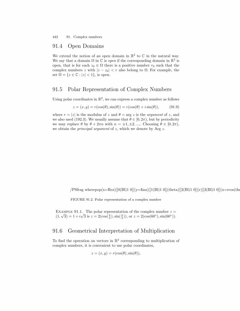
442 91. Complex numbers
91.4 Open Domains
We extend the notion of an open domain in R2 to C in the natural way.We say that a domain Ω in C is open if the corresponding domain in R2 isopen, that is for each z0 ∈ Ω there is a positive number r0 such that thecomplex numbers z with |z − z0| < r also belong to Ω. For example, theset Ω = z ∈ C : |z| < 1, is open.
91.5 Polar Representation of Complex Numbers
Using polar coordinates in R2, we can express a complex number as follows
z = (x, y) = r(cos(θ), sin(θ)) = r(cos(θ) + i sin(θ)), (91.9)
where r = |z| is the modulus of z and θ = arg z is the argument of z, andwe also used (192.3). We usually assume that θ ∈ [0, 2π), but by periodicitywe may replace θ by θ + 2πn with n = ±1,±2, ...,. Choosing θ ∈ [0, 2π),we obtain the principal argument of z, which we denote by Arg z.
/PSfrag wherepop(x=Rez)[[0(Bl)1 0]](y=Imz)[[1(Bl)1 0]](theta)[[2(Bl)1 0]](r)[[3(Bl)1 0]](x=rcos(theta))[[4(Bl)1 0]](y=rsin(theta))[[5(Bl)1 0]](z=(x,y)=r(cos(theta),sin(theta)))[[6(Bl)1 0]]7 0 1/Begin PSfraguserdict /PSfragpopputifelse
r
y=Imz
x=Reztheta
x=rcos(theta)
z=(x,y)=r(cos(theta),sin(theta))y=rsin(theta)
/End PSfrag /Hide PSfragPSfrag replacements/Unhide PSfrag– x = Re z˝ 0/Place PSfrag– y = Im z˝ 1/Place PSfrag– θ 2/Place PSfrag– r 3/Place PSfrag– x = r cos(θ)˝ 4/Place PSfrag– y = r sin(θ)˝ 5/Place PSfrag– z = (x, y) = r (cos(θ), sin(θ))˝ 6/Place PSfrag
FIGURE 91.2. Polar representation of a complex number
Example 91.1. The polar representation of the complex number z =(1,
√3) = 1+ i
√3 is z = 2(cos(π3 ), sin(
π3 )), or z = 2(cos(60), sin(60)).
91.6 Geometrical Interpretation of Multiplication
To find the operation on vectors in R2 corresponding to multiplication ofcomplex numbers, it is convenient to use polar coordinates,
z = (x, y) = r(cos(θ), sin(θ)),
91.7 Complex Conjugation 443
where r = |z| and θ = Arg z. Letting ζ = (ξ, η) = ρ(cos(φ), sin(φ)) be an-other complex number expressed using polar coordinates, the basic trigono-metric formulas from the Chapter Pythagoras and Euclid imply
zζ = r(cos(θ), sin(θ)) ρ(cos(φ), sin(φ))
= rρ(cos(θ) cos(φ)− sin(θ) sin(φ), cos(θ) sin(φ) + sin(θ) cos(φ))
= rρ(cos(θ + φ), sin(θ + φ)).
We conclude that multiplying z = r(cos(θ), sin(θ)) by ζ = ρ(cos(φ), sin(φ))corresponds to rotating the vector z the angle φ = Arg ζ, and changing itsmodulus by the factor ρ = |ζ|. In other words, we have
arg zζ = Arg z +Arg ζ, |zζ| = |z||ζ|. (91.10)
/PSfrag wherepop(x=Rez)[[0(Bl)1 0]](y=Imz)[[1(Bl)1 0]](z)[[2(Bl)1 0]](greekz)[[3(Bl)1 0]](zxgreekz)[[4(Bl)1 0]](—zxgreekz—=—z——greekz—)[[5(Bl)1 0]](Argzxgreekz=Argz+Arggreekz)[[6(Bl)1 0]]7 0 1/Begin PSfraguserdict /PSfragpopputifelse
z
1
y=Imz
x=Rez
greekz
zxgreekz
|zxgreekz|=|z||greekz|
Argzxgreekz=Argz+Arggreekz
/End PSfrag /Hide PSfragPSfrag replacements/Unhide PSfrag– x = Re z˝ 0/Place PSfrag– y = Im z˝ 1/Place PSfrag– z 2/Place PSfrag– ζ 3/Place PSfrag– z ζ4/Place PSfrag– |z ζ| = |z| |ζ|˝ 5/Place PSfrag– Arg z ζ = Arg z +Arg ζ˝ 6/Place PSfrag
FIGURE 91.3. Geometrical interpretation of multiplication of a complex numbers
Example 91.2. Multiplication by i corresponds to rotation counter-clockwise π
2 , or 90.
91.7 Complex Conjugation
If z = x+ iy is a complex number with x and y real, we define the complexconjugate z of z as
z = x− iy.
We see that z is real if and only if z = z and that z is purely imaginary,that is Re z = 0, if and only z = −z.Identifying C with R2, we see that complex conjugation corresponds
to reflection in the real axis. We also note the following relations, easily

444 91. Complex numbers
verified,
|z|2 = zz, Re z =1
2(z + z), Im z =
1
2i(z − z). (91.11)
91.8 Division
We extend the operation of division (denoted by /) of real numbers todivision of complex numbers by defining for w, u ∈ C with u = 0,
z = w/u =w
uif and only if uz = w.
To compute w/u for given w, u ∈ C with u = 0, we proceed as follows:
w/u =w
u=
wu
uu=
wu
|u|2.
Example 91.3. We have
1 + i
2 + i=
(1 + i)(2− i)
5=
3
5+ i
1
5.
Note that we consider complex numbers as scalars although they have alot in common with vectors in R2. The main reason for this is that ....
91.9 The Fundamental Theorem of Algebra
Consider a polynomial equation p(z) = 0, where p(z) = a0+a1z+ ...+anzn
is a polynomial in z of degree n with complex coefficients a0, ..., an. TheFundamental Theorem of Algebra states that the equation p(z) has at leastone complex root z1 satisfying p(z1) = 0. By the factorization algorithm,it follows that p(z) can be factored into
p(z) = (z − z1)p1(z),
where p1(z) is a polynomial of degree at most n−1. Indeed, the factorizationalgorithm from the Chapter Combinations of functions (Section 11.4) showsthat
p(z) = (z − z1)p1(z) + c,
where c is a constant. Setting z = z1, it follows that c = 0. Repeating theargument, we find that p(z) can be factored into
p(z) = c(z − z1)....(z − zn),
where z1, .., zn are the (complex valued in general) roots of p(z) = 0.
91.10 Roots 445
91.10 Roots
Consider the equation in w ∈ C
wn = z,
where n = 1, 2, .. is a natural number and z ∈ C is given. Using polarcoordinates with z = |z|(cos(θ), sin(θ)) ∈ C and w = |w|(cos(φ), sin(φ)) ∈C, the equation wn = z takes the form
|w|n(cos(nφ), sin(nφ)) = |z|(cos(θ), sin(θ))
from which it follows that
|w| = |z| 1n , φ =
θ
n+ 2π
k
n,
where k = 0, ..., n−1. We conclude that the equation wn = z has n distinctroots on the circle |w| = |z| 1
n . In particular, the equation w2 = −1 has thetwo roots w = ±i. The n roots of the equation wn = 1 are called the nroots of unity.
/PSfrag wherepop(z)[[0(Bl)1 0]](w1)[[1(Bl)1 0]](w2)[[2(Bl)1 0]](w3)[[3(Bl)1 0]](x=Rez)[[4(Bl)1 0]](y=Imz)[[5(Bl)1 0]](theta/2)[[6(Bl)1 0]](theta/3)[[7(Bl)1 0]]8 0 1/Begin PSfraguserdict /PSfragpopputifelse
z
1
z
1
y=Imz
x=Rez
y=Imz
x=Rez
w1
theta/2
w3
w2
w1
theta/3
w2
theta/2
/End PSfrag /Hide PSfragPSfrag replacements/Unhide PSfrag– z 0/Place PSfrag– w11/Place PSfrag– w22/Place PSfrag– w33/Place PSfrag– x = Re z˝ 4/Place PSfrag– y = Im z˝ 5/Place PSfrag– θ/2˝ 6/Place PSfrag– θ/3˝ 7/Place PSfrag
FIGURE 91.4. The “square” and “cubic” roots of z.
91.11 Solving a Quadratic Equationw2 + 2bw + c = 0
Consider the quadratic equation for w ∈ C,
w2 + 2bw + c = 0,
where b, c ∈ C. Completing the square, we get
(w + b)2 = b2 − c.
446 91. Complex numbers
If b2 − c ≥ 0 thenw = −b±
√b2 − c,
while if b2 − c < 0 then
w = −b± i√c− b2.
Chapter 91 Problems
91.1. Show that (a) 1i= −i, (b) i4 = 1.
91.2. Find (a) Re 11+i
, (b) Im 3+4i7−i
, (c) Im zz.
91.3. Let z1 = 4− 5i and z2 = 2+ 3i. Find in the form z = x+ iy (a) z1z2, (b)z1z2, (c) z1
z1+z2.
91.4. Show that the set of complex numbers z satisfying an equation of the form|z − z0| = r, where z0 ∈ C is given and r > 0, is a circle in the complex planewith center z0 and radius r.
91.5. Represent in polar form (a) 1 + i, (b) 1+i1−i
, (c) 2+3i5+4i
.
91.6. Solve the equations (a) z2 = i, (b) z8 = 1, (c) z2 + z + 1 = −i, (d)z4 − 3(1 + 2i)z2 + 6i = 0.
91.7. Determine the sets in the complex plane represented by (a) | z+iz−i
| = 1, (b)
Im z2 = 2, (c) |Arg z| ≤ π4.
91.8. Express z/w in polar coordinates in terms of the polar coordinates of zand w.
91.9. Describe in geometrical terms the mappings f : C → C given by (a)
f(z) = az + b, with a, b ∈ C, (b) f(z) = z2, (c) f(z) = z12 .
This is page 447Printer: Opaque this
92Analytic Geometry in Rn
I also think that the (mathematical) mine has become too deep andsooner or later it will be necessary to abandon it if new ore-bearingveins shall not be discovered. Physics and Chemistry display nowtreasures much more brilliant and easily exploitable, thus, appar-ently, everybody has turned completely in this direction, and possi-bly posts in Geometry in the Academy of Sciences will some day belike chairs in Arabic Language in universities at present. (Lagrange,1781)
92.1 Introduction and Survey of Basic Objectives
We now generalize the discussion of analytic geometry to Rn, where n isan arbitrary natural number. Following the pattern set above for R2 andR3, we define Rn to be the set of all possible ordered n-tuples of the form(x1, x2, ...., xn) with xi ∈ R for i = 1, ..., n. We refer to Rn as n-dimensionalEuclidean space.We all have a direct concrete experience of R3 as the three-dimensional
space of the real World, and we may think of R2 as an infinite flat sur-face, but we don’t have a similar experience with for example R4, exceptpossibly from some science fiction novel with space ships travelling in four-dimensional space-time. Actually, Einstein in his theory of relativity usedR4 as the set of space-time coordinates (x1, x2, x3, x4) with x4 = t repre-senting time, but of course had the same difficulty as we all have of “seeing”
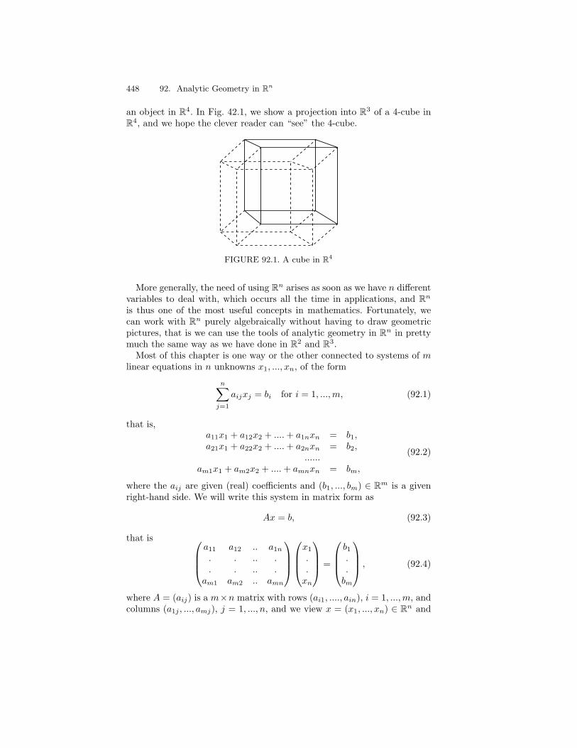
448 92. Analytic Geometry in Rn
an object in R4. In Fig. 42.1, we show a projection into R3 of a 4-cube inR4, and we hope the clever reader can “see” the 4-cube.
FIGURE 92.1. A cube in R4
More generally, the need of using Rn arises as soon as we have n differentvariables to deal with, which occurs all the time in applications, and Rn
is thus one of the most useful concepts in mathematics. Fortunately, wecan work with Rn purely algebraically without having to draw geometricpictures, that is we can use the tools of analytic geometry in Rn in prettymuch the same way as we have done in R2 and R3.Most of this chapter is one way or the other connected to systems of m
linear equations in n unknowns x1, ..., xn, of the form
n∑j=1
aijxj = bi for i = 1, ...,m, (92.1)
that is,a11x1 + a12x2 + ....+ a1nxn = b1,a21x1 + a22x2 + ....+ a2nxn = b2,
......am1x1 + am2x2 + ....+ amnxn = bm,
(92.2)
where the aij are given (real) coefficients and (b1, ..., bm) ∈ Rm is a givenright-hand side. We will write this system in matrix form as
Ax = b, (92.3)
that is a11 a12 .. a1n. . .. .. . .. .
am1 am2 .. amn
x1
.
.xn
=
b1..bm
, (92.4)
where A = (aij) is a m×n matrix with rows (ai1, ...., ain), i = 1, ...,m, andcolumns (a1j , ..., amj), j = 1, ..., n, and we view x = (x1, ..., xn) ∈ Rn and
92.1 Introduction and Survey of Basic Objectives 449
b = (b1, ..., bm) ∈ Rm as column vectors. We will also write the system inthe form
x1a1 + · · ·+ xnan = b, (92.5)
expressing the given column vector b ∈ Rm as a linear combination ofthe column vectors aj = (a1j , a2j , ..., amj), j = 1, 2, ..., n, with coefficients(x1, ..., xn). Notice that we use both (column) vectors in Rm (such as thecolumns of the matrix A and the right hand side b) and (column) vectorsin Rn such as the solution vector x.We shall view f(x) = Ax as a function or transformation f : Rn → Rm,
and we thus focus on a particular case of our general problem of solvingsystems of equations of the form f(x) = b, where f : Rn → Rm is thelinear transformation f(x) = Ax. We shall denote by R(A) the range off(x) = Ax, that is
R(A) = Ax ∈ Rm : x ∈ Rn = n∑
j=1
xjaj : xj ∈ R,
and by N(A) the null space of f(x) = Ax that is
N(A) = x ∈ Rn : Ax = 0 = x ∈ Rn :n∑
j=1
xjaj = 0.
We are interested in the question of existence and/or uniqueness of solu-tions x ∈ Rn to the problem Ax = b for a given m× n matrix A and righthand side b ∈ Rm. Of particular interest is the case m = n with as manyequations as unknowns.Existence of a solution x to Ax = b is of course the same as saying that
b ∈ R(A), which is the same as saying that b is a linear combination of thecolumns of A. Uniqueness is the same as saying that N(A) = 0, because ifx and x satisfy Ax = b and Ax = b, then by linearity, A(x − x) = 0, andif N(A) = 0 then x − x = 0 that is x = x. Further, the non-uniquenessof solutions of Ax = b is described by N(A): If Ax = b and Ax = b, thenx− x ∈ N(A).We may thus formulate the following prime objectives of our study of
the linear transformation f(x) = Ax given by the matrix A:
• Determine R(A).
• Determine N(A).
• Solve Ax = b for given b.
We state here the following partial answer given by the Fundamental The-orem of Linear Algebra, which we will prove in a couple of different waysbelow: Let m = n and suppose that N(A) = 0. Then Ax = b has a unique

450 92. Analytic Geometry in Rn
solution for any b ∈ Rm, that is, R(A) = Rm. In other words, if m = n,then uniqueness implies existence.In our study we will be led to concepts such as: linear combination,
linear span, linear space, vector space, subspace, linear independence, basis,determinant, linear transformation and projection, which we have alreadymet in the chapters on analytic geometry in R2 and R3 above.This chapter focusses mostly on theoretical issues while the computa-
tional methods such as Gaussian elimination and iterative methods areconsidered in more detail in Chapter Solving systems of linear equationsbelow.
92.2 Body/Soul and Artificial Intelligence
Before plunging into the geometry of Rn, we take a brake and return to thestory of Body and Soul which continues into our time with new questions:Is it possible to create computer programs for Artificial Intelligence AI,that is, can we give the computer some more or less advanced capability ofacting like an intelligent organism with some ability of “thinking”? It ap-pears that this question does not yet have a clear positive answer, despitemany dreams in that direction during the development of the computer.In seeking an answer, Spencer’s principle of adaptivity of course plays animportant role: an intelligent system must be able to adapt to changes inits environment. Further, the presence of a goal or final cause accordingto Leibniz, seems to be an important feature of intelligence, to judge if anaction of a system is stupid or not. Below we will design adaptive IVP-solvers, which are computer programs for solving systems of differentialequations, with features of adaptive feed-back from the computational pro-cess towards the goal of error control. These IVP-solvers thus show somekind of rudiments of intelligence, and at any rate are infinitely much more“clever” than traditional non-adaptive IVP-solvers with no feed-back.
92.3 The Vector Space Structure of Rn
We view Rn as a vector space consisting of vectors which are ordered n-tuples, x = (x1, ...., xn) with components xi ∈ R, i = 1, ..., n. We writex = (x1, ...., xn) for short, and refer to x ∈ Rn as a vector with componentxi in position i.We may add two vectors x = (x1, ...., xn) and y = (y1, ...., yn) in Rn by
componentwise addition to get a new vector x+ y in Rn defined by
x+ y = (x1 + y1, x2 + y2, ...., xn + yn). (92.6)
Further, we may multiply a vector x = (x1, ...., xn) by a real number λ bycomponentwise multiplication with λ, to get a new vector λx in Rn defined

92.4 The Scalar Product and Orthogonality 451
byλx = (λx1, ..., λxn). (92.7)
The operations of adding two vectors in Rn and multiplying a vectorin Rn with a real number, of course directly generalize the correspondingoperations from the cases n = 2 and n = 3 considered above. The gener-alization helps us to deal with Rn using concepts and tools which we havefound useful in R2 and R3.We may thus add vectors in Rn and multiply them by real numbers
(scalars), the usual commutative and distributive rules hold for these op-erations, and Rn is thus a vector space. We say that (0, 0, .., 0) is the zerovector in Rn and write 0 = (0, 0, .., 0).Linear algebra concerns vectors in vector spaces, also refereed to as linear
spaces, and linear functions of vectors, that is linear transformations ofvectors. As we just saw, Rn is a vector space, but there are also manyother types of vector spaces, where the vectors have a different nature. Inparticular, we will below meet vector spaces consisting of vectors whichare functions. In this chapter we focus on Rn, the most basic of all vectorspaces. We know that linear transformations in R2 and R3 lead to 2 × 2and 3 × 3 matrices, and we shall now generalize to linear transformationsfrom Rn into Rm which can be represented by m× n matrices.We give in this chapter a condensed (and dry) presentation of some basic
facts of linear algebra in Rn. Many applications of the theoretical resultspresented will appear in the rest of the book.
92.4 The Scalar Product and Orthogonality
We define the scalar product x · y = (x, y) of two vectors x and y in Rn, by
x · y = (x, y) =n∑
i=1
xiyi. (92.8)
This generalizes the scalar product in R2 and R3. Note that here we intro-duce a new notation for the scalar product of two vectors x and y, namely(x, y), as an alternative to the “dot product” x · y used in R2 and R3. Weshould be ready to use both notations.The scalar product is bilinear in the sense that (x+y, z) = (x, z)+(y, z),
(λx, z) = λ(x, z), (x, y + z) = (x, y) + (x, z) and (x, λy) = λ(x, y), andsymmetric in the sense that (x, y) = (y, x), for all vectors x, y, z ∈ Rn andλ ∈ R.We say that two vectors x and y in Rn are orthogonal if (x, y) = 0. We
define
|x| = (n∑
i=1
x2i )
1/2 = (x, x)1/2 (92.9)

452 92. Analytic Geometry in Rn
to be the Euclidean length or norm of the vector x. Note that this definitionof length is a direct generalization of the natural length |x| of a vector x inRn, n = 1, 2, 3.
Example 92.1. Let x = (2,−4, 5, 1, 3) and y = (1, 4, 6,−1, 2) be twovectors in R5. We compute (x, y) = 2×1+(−4)×4+5×6+1× (−1)+3× 2 = 21.
92.5 Cauchy’s Inequality
Cauchy’s inequality states that for x, y ∈ Rn,
|(x, y)| ≤ |x| |y|.
In words: the absolute value of the scalar product of two vectors is boundedby the product of the norms of the vectors. We prove Cauchy’s inequalityby noting that for all s ∈ R,
0 ≤ |x+ sy|2 = (x+ sy, x+ sy) = |x|2 + 2s(x, y) + s2|y|2,
and then assuming that y = 0, choosing s = −(x, y)/|y|2 (which minimizesthe right-hand side), to get
0 ≤ |x|2 − 2(x, y)2
|y|2+
(x, y)2
|y|2= |x|2 − (x, y)2
|y|2,
which proves the desired result.We recall that for n = 2, 3,
(x, y) = x · y = cos(θ)|x||y|,
where θ is the angle between x and y, from which of course Cauchy’sinequality follows directly using the fact that | cos(θ)| ≤ 1.We define the angle θ ∈ [0, 2π) between two non-zero vectors x and y in
Rn by
cos(θ) =(x, y)
|x||y|, (92.10)
which generalizes the corresponding notion for n = 2, 3.
Example 92.2. The angle between the vectors x = (1, 2, 3, 4) andy = (4, 3, 2, 1) in R4 is equal to arccos 2
3 ≈ 0.8411 ≈ 48 since (x, y) = 20
and |x| = |y| =√30.

92.6 The Linear Combinations of a Set of Vectors 453
92.6 The Linear Combinations of a Set of Vectors
We know that two non-parallel vectors a1 and a2 in R3 define a plane in R3
through the origin consisting of all the linear combinations λ1a1+λ2a2 withcoefficients λ1 and λ2 in R. The normal to the plane is given by a1 × a2. Aplane through the origin is an example of subspace of R3, which is a subsetof R with the property that vector addition and scalar multiplication doesnot lead outside the set. So, a subset S of R3 is a subspace if the sum ofany two vectors in S belongs to S and scalar multiplication of a vector inS gives a vector in S. Clearly, a plane through the origin is a subspace ofR3. Similarly, a line through the origin defined as the scalar multiples λ1a1with coefficients λ1 ∈ R and a1 a given vector in R3, is a subspace of R3.The subspaces of R3 consist of lines and planes through the origin. Noticethat a plane or line in R3 not passing through the origin, is not a subspace.More generally, we use the concept of a vector space to denote a set of
vectors for which the operations of vector addition and scalar multiplicationdoes not lead outside the set. Of course, R3 is a vector space. A subspaceof R3 is a vector space. A plane or line in R3 through the origin is a vectorspace. The concept of vector space is fundamental in mathematics and wewill meet this term many times below.We will now generalize to Rm with m > 3 and we will then meet new
examples of vector spaces and subspaces of vector spaces. Let a1, a2,...,an,be n non-zero vectors in Rm. A vector b in Rm of the form
b = λ1a1 + λ2a2 + · · ·+ λnan, (92.11)
where the λi ∈ R, is said to be a linear combination of the set of vectorsa1, ..., an with coefficients λ1, ..., λn. If
c = µ1a1 + µ2a2 + · · ·+ µnan, (92.12)
is another linear combination of a1, ..., an with coefficients µj ∈ R, thenthe vector
b+ c = (λ1 + µ1)a1 + (λ2 + µ2)a2 + · · ·+ (λ+µn)an, (92.13)
is again a linear combination of a1, ..., am now with coefficients λj + µj .Further, for any α ∈ R the vector
αb = αλ1a1 + αλ2a2 + · · ·+ αλmam (92.14)
is also a linear combination of a1, ..., am with coefficients αλj . This meansthat if we let S(a1, ...an) denote the set of all linear combinations
λ1a1 + λ2a2 + · · ·+ λnan, (92.15)
of a1, ..., an, where the coefficients λj ∈ R, then S(a1, ...an) is indeed avector space, since vector addition and multiplication by scalars do not lead
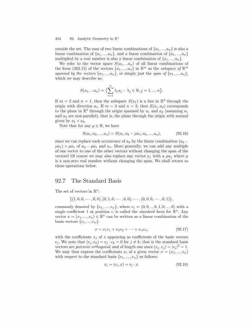
454 92. Analytic Geometry in Rn
outside the set. The sum of two linear combinations of a1, ..., an is also alinear combination of a1, ..., an, and a linear combination of a1, ..., anmultiplied by a real number is also a linear combination of a1, ..., an.We refer to the vector space S(a1, ...an) of all linear combinations of
the form (202.15) of the vectors a1, ..., an in Rm as the subspace of Rm
spanned by the vectors a1, ..., an, or simply just the span of a1, ..., an,which we may describe as:
S(a1, ...an) = n∑i=1
λjaj : λj ∈ R, j = 1, ..., n.
If m = 2 and n = 1, then the subspace S(a1) is a line in R2 through theorigin with direction a1. If m = 3 and n = 2, then S(a1, a2) correspondsto the plane in R3 through the origin spanned by a1 and a2 (assuming a1and a2 are non-parallel), that is, the plane through the origin with normalgiven by a1 × a2.Note that for any µ ∈ R, we have
S(a1, a2, ..., an) = S(a1, a2 − µa1, a3, ..., an), (92.16)
since we can replace each occurrence of a2 by the linear combination (a2 −µa1) + µa1 of a2 − µa1 and a1. More generally, we can add any multipleof one vector to one of the other vectors without changing the span of thevectors! Of course we may also replace any vector aj with a µaj where µis a non-zero real number without changing the span. We shall return tothese operations below.
92.7 The Standard Basis
The set of vectors in Rn:
(1, 0, 0, · · · , 0, 0), (0, 1, 0, · · · , 0, 0), · · · , (0, 0, 0, · · · , 0, 1) ,
commonly denoted by e1, ...., en, where ei = (0, 0, .., 0, 1, 0, ..., 0) with asingle coefficient 1 at position i, is called the standard basis for Rn. Anyvector x = (x1, ..., xn) ∈ Rn can be written as a linear combination of thebasis vectors e1, ..., en:
x = x1e1 + x2e2 + · · ·+ xnen, (92.17)
with the coefficients xj of x appearing as coefficients of the basis vectorsej . We note that (ej , ek) = ej · ek = 0 for j = k, that is the standard basisvectors are pairwise orthogonal, and of length one since (ej , ej) = |ej |2 = 1.We may thus express the coefficients xi of a given vector x = (x1, ..., xn)with respect to the standard basis e1, ...., en as follows:
xi = (ei, x) = ei · x. (92.18)
92.8 Linear Independence 455
92.8 Linear Independence
We recall that to specify a plane in R3 as the set of linear combinations oftwo given vectors a1 and a2, we assume that a1 and a2 are non-parallel.The generalization of this condition to a set a1, ..., am of m vectors inRn, is referred to as linear independence, which we now proceed to define.Eventually, this will lead us to the concept of basis of a vector space, whichis one of the most basic(!) concepts of linear algebra.A set a1, ..., an of vectors in Rm is said to be linearly independent if
none of the vectors ai can be expressed as a linear combination of theothers. Conversely, if some of the vectors ai can be expressed as a linearcombination of the others, for example if
a1 = λ2a2 + ...+ λnan (92.19)
for some numbers λ2,...,λn, we say that the set a1, a2, ..., an is linearlydependent. As a test of linear independence of a1, a2, ..., an, we can use:if
λ1a1 + λ2a2 + ...+ λnan = 0 (92.20)
implies that λ1 = λ2 = .... = λn = 0, then a1, a2, ..., an is linearlyindependent. This is because if (202.20) holds with some of the λj differentfrom 0, for example, λ1 = 0, then we could divide by λ1 and express a1 asa linear combination of a2, ..., am:
a1 = −λ2
λ1a2 + ...+−λn
λ1an. (92.21)
The standard basis e1, ..., en is (of course) a linearly independent set,since if
λ1e1 + ....+ λnen = 0,
then λi = 0 for i = 1, ..., n, because 0 = (0, 0, ..., 0) = λ1e1 + .... + λnen =(λ1, ..., λn).
92.9 Reducing a Set of Vectors to get a Basis
Consider the subspace S(a1, ..., an) spanned by the set of vectors a1, a2, ...,an. If the set a1, a2, ..., an is linearly dependent, say that an can beexpressed as a linear combination of a1, ..., an−1, then S(a1, ..., an) is infact spanned by a1, ..., an−1 and thus S(a1, ..., an) = S(a1, ..., an−1). Thisfollows simply by replacing all occurrences of an by its linear combination ofa1, ..., an−1. Continuing this way, eliminating linearly dependent vectors,we may express S(a1, ..., an) as the span of a1, a2, ..., ak (with a suitableenumeration), that is, S(a1, ..., an) = S(a1, a2, ..., ak, where k ≤ n, and theset a1, a2, ..., ak is linearly independent. This means that a1, a2, ..., ak is
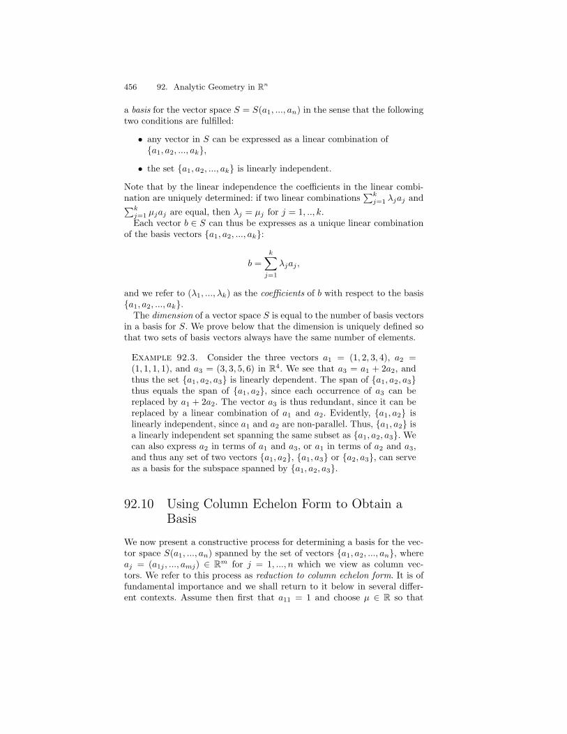
456 92. Analytic Geometry in Rn
a basis for the vector space S = S(a1, ..., an) in the sense that the followingtwo conditions are fulfilled:
• any vector in S can be expressed as a linear combination ofa1, a2, ..., ak,
• the set a1, a2, ..., ak is linearly independent.
Note that by the linear independence the coefficients in the linear combi-nation are uniquely determined: if two linear combinations
∑kj=1 λjaj and∑k
j=1 µjaj are equal, then λj = µj for j = 1, .., k.Each vector b ∈ S can thus be expresses as a unique linear combination
of the basis vectors a1, a2, ..., ak:
b =k∑
j=1
λjaj ,
and we refer to (λ1, ..., λk) as the coefficients of b with respect to the basisa1, a2, ..., ak.The dimension of a vector space S is equal to the number of basis vectors
in a basis for S. We prove below that the dimension is uniquely defined sothat two sets of basis vectors always have the same number of elements.
Example 92.3. Consider the three vectors a1 = (1, 2, 3, 4), a2 =(1, 1, 1, 1), and a3 = (3, 3, 5, 6) in R4. We see that a3 = a1 + 2a2, andthus the set a1, a2, a3 is linearly dependent. The span of a1, a2, a3thus equals the span of a1, a2, since each occurrence of a3 can bereplaced by a1 + 2a2. The vector a3 is thus redundant, since it can bereplaced by a linear combination of a1 and a2. Evidently, a1, a2 islinearly independent, since a1 and a2 are non-parallel. Thus, a1, a2 isa linearly independent set spanning the same subset as a1, a2, a3. Wecan also express a2 in terms of a1 and a3, or a1 in terms of a2 and a3,and thus any set of two vectors a1, a2, a1, a3 or a2, a3, can serveas a basis for the subspace spanned by a1, a2, a3.
92.10 Using Column Echelon Form to Obtain aBasis
We now present a constructive process for determining a basis for the vec-tor space S(a1, ..., an) spanned by the set of vectors a1, a2, ..., an, whereaj = (a1j , ..., amj) ∈ Rm for j = 1, ..., n which we view as column vec-tors. We refer to this process as reduction to column echelon form. It is offundamental importance and we shall return to it below in several differ-ent contexts. Assume then first that a11 = 1 and choose µ ∈ R so that
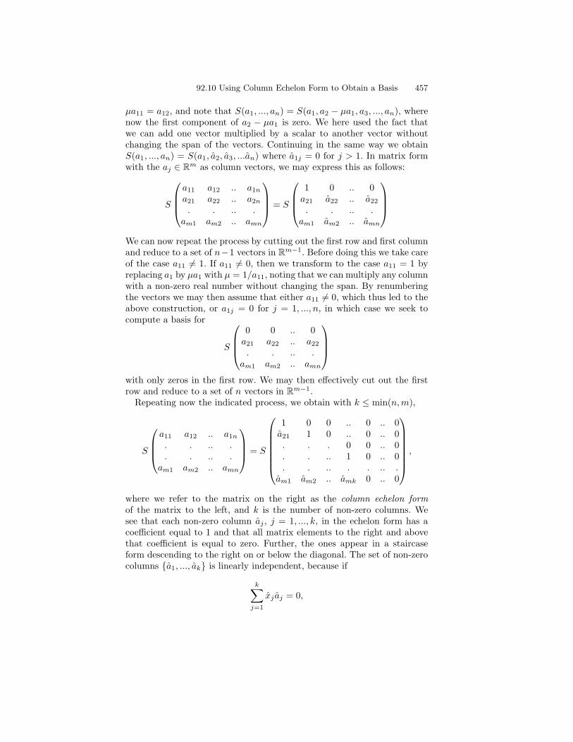
92.10 Using Column Echelon Form to Obtain a Basis 457
µa11 = a12, and note that S(a1, ..., an) = S(a1, a2 − µa1, a3, ..., an), wherenow the first component of a2 − µa1 is zero. We here used the fact thatwe can add one vector multiplied by a scalar to another vector withoutchanging the span of the vectors. Continuing in the same way we obtainS(a1, ..., an) = S(a1, a2, a3, ...an) where a1j = 0 for j > 1. In matrix formwith the aj ∈ Rm as column vectors, we may express this as follows:
S
a11 a12 .. a1na21 a22 .. a2n. . .. .
am1 am2 .. amn
= S
1 0 .. 0a21 a22 .. a22. . .. .
am1 am2 .. amn
We can now repeat the process by cutting out the first row and first columnand reduce to a set of n−1 vectors in Rm−1. Before doing this we take careof the case a11 = 1. If a11 = 0, then we transform to the case a11 = 1 byreplacing a1 by µa1 with µ = 1/a11, noting that we can multiply any columnwith a non-zero real number without changing the span. By renumberingthe vectors we may then assume that either a11 = 0, which thus led to theabove construction, or a1j = 0 for j = 1, ..., n, in which case we seek tocompute a basis for
S
0 0 .. 0a21 a22 .. a22. . .. .
am1 am2 .. amn
with only zeros in the first row. We may then effectively cut out the firstrow and reduce to a set of n vectors in Rm−1.Repeating now the indicated process, we obtain with k ≤ min(n,m),
S
a11 a12 .. a1n. . .. .. . .. .
am1 am2 .. amn
= S
1 0 0 .. 0 .. 0a21 1 0 .. 0 .. 0. . . 0 0 .. 0. . .. 1 0 .. 0. . .. . . .. .
am1 am2 .. amk 0 .. 0
,
where we refer to the matrix on the right as the column echelon formof the matrix to the left, and k is the number of non-zero columns. Wesee that each non-zero column aj , j = 1, ..., k, in the echelon form has acoefficient equal to 1 and that all matrix elements to the right and abovethat coefficient is equal to zero. Further, the ones appear in a staircaseform descending to the right on or below the diagonal. The set of non-zerocolumns a1, ..., ak is linearly independent, because if
k∑j=1
xj aj = 0,

458 92. Analytic Geometry in Rn
then we get successively x1 = 0, x2 = 0,..., xk = 0, and thus a1, ..., akforms a basis for S(a1, ..., an). The dimension of S(a1, ..., an) is equal to k.If zero columns appear in the echelon form, then the original set a1, ..., anis linearly dependent.We note that, because of the construction, zero columns must appear if
n > m, and we thus understand that a set of n vectors in Rm is linearlydependent if n > m. We may also understand that if n < m, then theset a1, ..., an cannot span Rm, because if k < m, then there are vectorsb ∈ Rm which cannot be expressed as linear combinations of a1, ..., ak aswe now show: if
b =k∑
j=1
xj aj ,
then the coefficients x1, ..., xk are determined by the coefficients b1, ..., bk, ofb occurring in the rows with the coefficient 1. For example, in the case the1s appear on the diagonal, we first compute x1 = b1, then x2 = b1 − a21x1
etc, and thus the remaining coefficients bk+1, ..., bm of b cannot be arbitrary.
92.11 Using Column Echelon Form to Obtain R(A)
By reduction to column echelon form we can construct a basis for R(A) fora given m× n matrix A with column vectors a1, ..., an because
Ax =
n∑j=1
xjaj
and thus R(A) = S(a1, ..., an) expressing that the range R(A) = Ax : x ∈Rn is equal to the vector space S(a1, ..., an) of all linear combinations ofthe set of column vectors a1, ..., an. Setting now
A =
a11 a12 .. a1n. . .. .. . .. .
am1 am2 .. amn
, A =
1 0 0 .. 0 .. 0a21 1 0 .. 0 .. 0. . . 0 0 .. 0. . .. 1 0 .. 0. . .. . . .. .
am1 am2 .. amk 0 .. 0
with A obtained from A by reduction to column echelon form, we have
R(A) = R(A) = S(a1, ..., ak),
and thus a1, ..., ak forms a basis for R(A). In particular we can easilycheck if a given vector b ∈ Rm belongs to R(A), by using the echelonform. By reduction to column echelon form we can thus give an answer
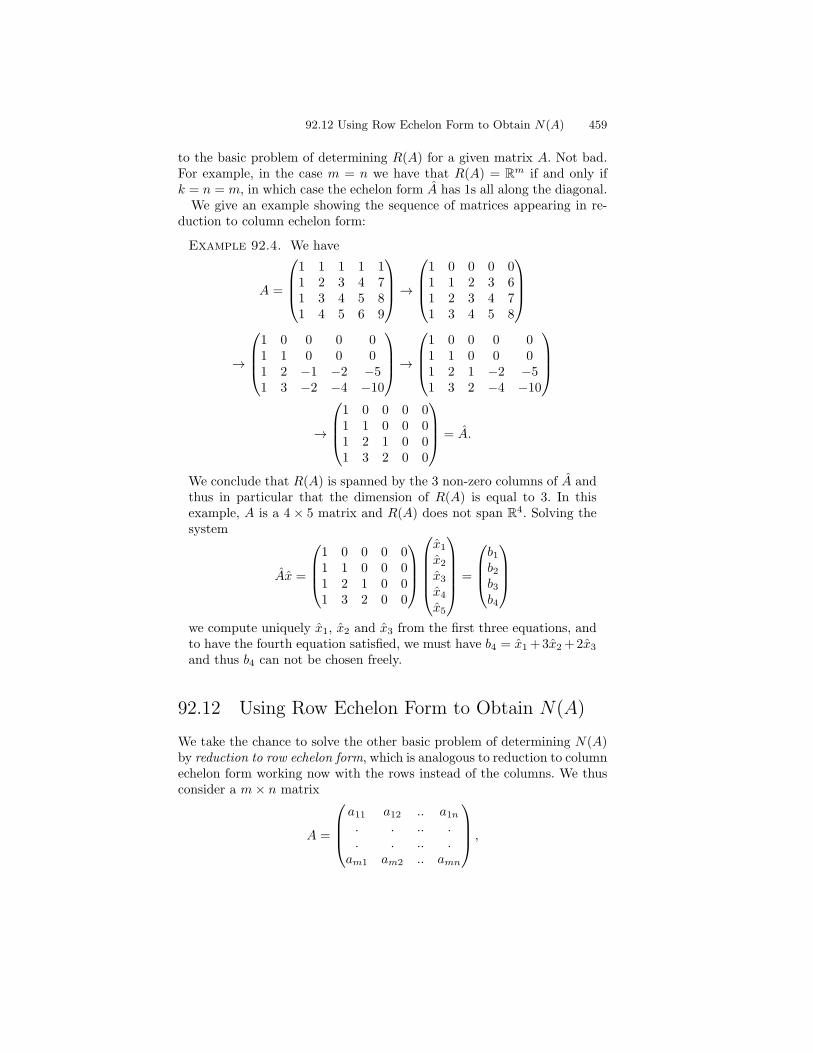
92.12 Using Row Echelon Form to Obtain N(A) 459
to the basic problem of determining R(A) for a given matrix A. Not bad.For example, in the case m = n we have that R(A) = Rm if and only ifk = n = m, in which case the echelon form A has 1s all along the diagonal.We give an example showing the sequence of matrices appearing in re-
duction to column echelon form:
Example 92.4. We have
A =
1 1 1 1 11 2 3 4 71 3 4 5 81 4 5 6 9
→
1 0 0 0 01 1 2 3 61 2 3 4 71 3 4 5 8
→
1 0 0 0 01 1 0 0 01 2 −1 −2 −51 3 −2 −4 −10
→
1 0 0 0 01 1 0 0 01 2 1 −2 −51 3 2 −4 −10
→
1 0 0 0 01 1 0 0 01 2 1 0 01 3 2 0 0
= A.
We conclude that R(A) is spanned by the 3 non-zero columns of A andthus in particular that the dimension of R(A) is equal to 3. In thisexample, A is a 4 × 5 matrix and R(A) does not span R4. Solving thesystem
Ax =
1 0 0 0 01 1 0 0 01 2 1 0 01 3 2 0 0
x1
x2
x3
x4
x5
=
b1b2b3b4
we compute uniquely x1, x2 and x3 from the first three equations, andto have the fourth equation satisfied, we must have b4 = x1+3x2+2x3
and thus b4 can not be chosen freely.
92.12 Using Row Echelon Form to Obtain N(A)
We take the chance to solve the other basic problem of determining N(A)by reduction to row echelon form, which is analogous to reduction to columnechelon form working now with the rows instead of the columns. We thusconsider a m× n matrix
A =
a11 a12 .. a1n. . .. .. . .. .
am1 am2 .. amn
,
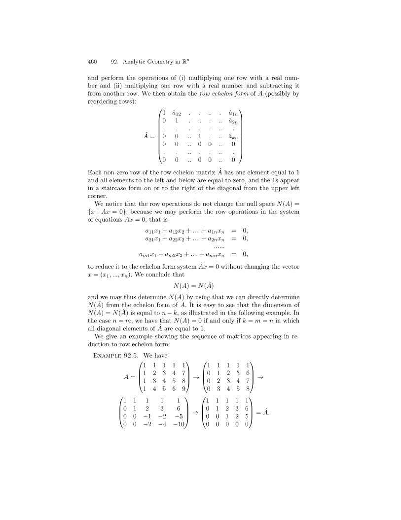
460 92. Analytic Geometry in Rn
and perform the operations of (i) multiplying one row with a real num-ber and (ii) multiplying one row with a real number and subtracting itfrom another row. We then obtain the row echelon form of A (possibly byreordering rows):
A =
1 a12 . . .. . a1n0 1 . .. . .. a2n. . . . . .. .0 0 .. 1 . .. akn0 0 .. 0 0 .. 0. . .. . . .. .0 0 .. 0 0 .. 0
Each non-zero row of the row echelon matrix A has one element equal to 1and all elements to the left and below are equal to zero, and the 1s appearin a staircase form on or to the right of the diagonal from the upper leftcorner.We notice that the row operations do not change the null space N(A) =
x : Ax = 0, because we may perform the row operations in the systemof equations Ax = 0, that is
a11x1 + a12x2 + ....+ a1nxn = 0,a21x1 + a22x2 + ....+ a2nxn = 0,
......am1x1 + am2x2 + ....+ amnxn = 0,
to reduce it to the echelon form system Ax = 0 without changing the vectorx = (x1, ..., xn). We conclude that
N(A) = N(A)
and we may thus determine N(A) by using that we can directly determineN(A) from the echelon form of A. It is easy to see that the dimension ofN(A) = N(A) is equal to n− k, as illustrated in the following example. Inthe case n = m, we have that N(A) = 0 if and only if k = m = n in whichall diagonal elements of A are equal to 1.We give an example showing the sequence of matrices appearing in re-
duction to row echelon form:
Example 92.5. We have
A =
1 1 1 1 11 2 3 4 71 3 4 5 81 4 5 6 9
→
1 1 1 1 10 1 2 3 60 2 3 4 70 3 4 5 8
→
1 1 1 1 10 1 2 3 60 0 −1 −2 −50 0 −2 −4 −10
→
1 1 1 1 10 1 2 3 60 0 1 2 50 0 0 0 0
= A.

92.13 Gaussian Elimination 461
We now determine N(A) by determining N(A) = N(A) by seeking thesolutions x = (x1, ..., x5) of the system Ax = 0, that is
1 1 1 1 10 1 2 3 60 0 1 2 50 0 0 0 0
x1
x2
x3
x4
x5
=
0000
.
We see that we can freely choose x4 and x5 and then solve for x3, x2
and x1 to get the solution in the form
x = λ1
01−210
+ λ2
04−501
where λ1 and λ2 are any real numbers. We have now computed a basisfor N(A) and we see in particular that the dimension of N(A) is equalto 2. We recall that the dimension of R(A) is equal to 3 and we notethat the sum of the dimensions of R(A) and N(A) happens to be equalto 5 that is the number of columns of A. This is a general fact whichwe prove in the Fundamental Theorem below.
92.13 Gaussian Elimination
Gaussian elimination to compute solutions to the systema11 a12 .. a1n. . .. .. . .. .
am1 am2 .. amn
x1
.
.xn
=
b1..bm
closely couples to reduction to row echelon form. Performing row operationswe may reduce to a system of the form
A =
1 a12 . . .. . a1n0 1 . .. . .. a2n. . . . . .. .0 0 .. 1 . .. akn0 0 .. 0 0 .. 0. . .. . . .. .0 0 .. 0 0 .. 0
x1
.
.xn
=
b1..
bm
with the same solution vector x. We may assume, by possibly by renum-bering the components of x, that the 1s appear on the diagonal. We see

462 92. Analytic Geometry in Rn
that solvability is equivalent to having bj = 0 for j = k + 1, ..,m, and thenon-uniqueness is expressed by N(A) as explained above. In the casem = nwe have that N(A) = 0 if and only if k = m = n in which case all diagonal
elements of A are equal to 1, and the system Ax = b is uniquely solv-able for all b ∈ Rm, and thus Ax = b is uniquely solvable for all b ∈ Rm.We conclude that if m = n, then uniqueness implies existence. We maythus say that by Gaussian elimination or reduction to row echelon form,we may solve our basic problems of existence and uniqueness of solutionsto the system Ax = b. We shall add more information on these problemsin the Fundamental Theorem of Linear Algebra below. For more informa-tion on Gaussian elimination, we refer to Chapter Solving Linear AlgebraicSystems below.
92.14 A Basis for Rn Contains n Vectors
Let us now prove that if a1, ..., am is a basis for Rn, then m = n, thatis any basis for Rn has exactly n elements, no more no less. We alreadydeduced this fact from the column echelon form above, but we here give a“coordinate-free” proof which applies to more general situations.We recall that a set a1, ..., am of vectors in Rn is a basis for Rn if the
following two conditions are fulfilled:
• a1, ..., am is linearly independent,
• any vector x ∈ Rn can be expressed as a linear combination x =∑mj=1 λjaj of a1, ..., am with coefficients λj .
Of course, e1, ..., en is a basis for Rn in this sense.To prove that m = n, we consider the set e1, a1, a2, ..., am. Since
a1, ..., am is a basis for Rn, that is spans Rn, the vector e1 can be ex-pressed as a linear combination of a1, ..., am:
e1 =m∑j=1
λjaj ,
with some λj = 0. Suppose λ1 = 0. Then, dividing by λ1 expresses a1as a linear combination of e1, a2, ..., am. This means that e1, a2, ..., amspans Rn. Consider now the set e1, e2, a2, ..., am. The vector e2 can beexpressed as a linear combination of e1, a2, ..., am and some of the coef-ficients of the aj must be non-zero, since e1, e2 are linearly independent.Supposing the coefficient of a2 is non-zero, we can eliminate a2 and thusthe set e1, e2, a3, ..., am now spans Rn. Continuing this way we get the sete1, e2, ..., en, an+1, ..., am if m > n and the set e1, e2, ..., en if m = n,which both span Rn. We conclude that m ≥ n, since if e.g. m = n − 1,

92.15 Coordinates in Different Bases 463
we would end up with the set e1, e2, ..., en−1 which does not span Rn
contrary to the assumption.Repeating this argument with the roles of the basis e1, e2, ..., en and
a1, a2, ..., am interchanged, we get the reverse inequality n ≥ m and thusn = m. Of course, intuitively, there are n independent directions in Rn andthus a basis of Rn has n elements, no more no less.We also note that if a1, ..., am is a linearly independent set in Rn, then
it can be extended to a basis a1, ..., am, am+1, .., an by adding suitableelements am+1,..,an. The extension starts by adding am+1 as any vectorwhich cannot be expressed as a linear combination of the set a1, ..., am.Then a1, ..., am, am+1 is linearly independent, and if m + 1 < n, theprocess may be continued.We summarize as follows:
Theorem 92.1 Any basis of Rn has n elements. Further, a set of n vectorsin Rn span Rn if and only if it is linearly independent, that is a set of nvectors in Rn that spans Rn or is independent, must be a basis. Also, a setof fewer than n vectors in Rn cannot span Rn, and a set of more than nvectors in Rn must be linearly dependent.
The argument used to prove this result can also be used to prove thatthe dimension of a vector space S is well defined in the sense that any twobases have the same number of elements.
92.15 Coordinates in Different Bases
There are many different bases in Rn if n > 1 and the coordinates ofa vector with respect to one basis are not equal to the coordinates withrespect to another basis.Suppose a1, ..., an is a basis for Rn and let us seek the connection
between the coordinates of one and the same vector in the standard basise1, ..., en and the basis a1, ..., an. Assume then that the coordinates ofthe basis vectors aj in the standard basis e1, ..., en are given by aj =(a1j , ...anj) for j = 1, ...n, that is
aj =n∑
i=1
aijei.
Denoting the coordinates of a vector x with respect to e1, ..., en by xj
and the coordinates with respect to a1, ..., an by xj , we have
x =
n∑j=1
xjaj =
n∑j=1
xj
n∑i=1
aijei =
n∑i=1
(
n∑j=1
aij xj)ei, (92.22)

464 92. Analytic Geometry in Rn
that is since also x =∑n
i=1 xiei and the coefficients xi of x are unique,
xi =n∑
j=1
aij xj for i = 1, ...n. (92.23)
This relation expresses the connection between the coordinates xj withrespect to the basis a1, ..., an, and the coordinates xi with respect tothe standard basis e1, ..., en, in terms of the coordinates aij of the basisvectors aj with respect to e1, ..., en. This is a basic connection, which willplay a central role in the development to come.Using the scalar product we can express the coordinates aij of the basis
vector aj as aij = (ei, aj). To find the connection (202.23) between thecoordinates xj with respect to the basis a1, ..., an, and the coordinatesxi with respect to the standard basis e1, ..., en, we may start from theequality
∑nj=1 xjej = x =
∑nj=1 xjaj and take the scalar product of both
sides with ei, to get
xi =n∑
j=1
xj(ei, aj) =n∑
j=1
aij xj , (92.24)
where aij = (ei, aj).
Example 92.6. The set a1, a2, a3 with a1 = (1, 0, 0), a2 = (1, 1, 0),a3 = (1, 1, 1) in the standard basis, forms a basis for R3 since the seta1, a2, a3 is linearly independent. This is because if λ1a1 + λ2a2 +λ3a3 = 0, then λ3 = 0 and thus also λ2 = 0 and thus also λ1 = 0.If (x1, x2, x3) are the coordinates with respect to the standard basisand (x1, x2, x3) are the coordinates with respect to a1, a2, a3 of acertain vector, then the connection between the coordinates is given by(x1, x2, x3) = x1a1 + x2a2 + x3a3 = (x1 + x2 + x3, x2 + x3, x3). Solvingfor the xj in terms of the xi, we get (x1, x2, x3) = (x1−x2, x2−x3, x3).
92.16 Linear Functions f : Rn → RA linear function f : Rn → R satisfies
f(x+y) = f(x)+f(y), f(αx) = αf(x) for all x, y ∈ Rn, α ∈ R. (92.25)
We say that f(x) is a scalar linear function since f(x) ∈ R. Expressingx = x1e1 + ... + xnen in the standard basis e1, ..., en, and using thelinearity of f(x), we find that
f(x) = x1f(e1) + ....+ xnf(en), (92.26)

92.17 Linear Transformations f : Rn → Rm 465
and thus f(x) has the form
f(x) = f(x1, ..., xn) = a1x1 + a2x2 + ....+ anxn, (92.27)
where the aj = f(ej) are real numbers. We can write f(x) as
f(x) = (a, x) = a · x, (92.28)
where a = (a1, ..., an) ∈ Rn, that is f(x) can be expressed as the scalarproduct of x with the vector a ∈ Rn with components aj given by aj =f(ej).The set of scalar linear functions is the mother of all other functions. We
now generalize to systems of scalar linear functions. Linear algebra is thestudy of systems of linear functions.
Example 92.7. f(x) = 2x1 + 3x2 − 7x3 defines a linear functionf : R3 → R with coefficients f(e1) = a1 = 2, f(e2) = a2 = 3 andf(e3) = a3 = −7.
92.17 Linear Transformations f : Rn → Rm
A function f : Rn → Rm is said to be linear if
f(x+y) = f(x)+f(y), f(αx) = αf(x) for all x, y ∈ Rn, α ∈ R. (92.29)
We also refer to a linear function f : Rn → Rm as a linear transformationof Rn into Rm.The image f(x) of x ∈ Rn is a vector in Rm with components which
we denote by fi(x), i = 1, 2, ...,m, so that f(x) = (f1(x), ..., fm(x)). Eachcoordinate function fi(x) is a linear scalar function fi : Rn → R if f : Rn →Rm is linear. We can thus represent a linear transformation f : Rn → Rm
asf1(x) = a11x1 + a12x2 + ....+ a1nxn
f2(x) = a21x1 + a22x2 + ....+ a2nxn
......fm(x) = am1x1 + am2x2 + ....+ amnxn
(92.30)
with the coefficients aij = fi(ej) = (ei, f(ej)) ∈ R.We can write (202.30) in condensed form as
fi(x) =n∑
j=1
aijxj for i = 1, ...,m. (92.31)
Example 92.8. f(x) = (2x1 + 3x2 − 7x3, x1 + x3) defines a linearfunction f : R3 → R2 with coefficients f1(e1) = a11 = 2, f1(e2) =a12 = 3 and f1(e3) = a13 = −7, f2(e1)a21 = 1, f2(e2)a22 = 0 andf2(e3) = a23 = 1.
466 92. Analytic Geometry in Rn
92.18 Matrices
We now return to the notion of a matrix and develop a matric calculus.The connection to linear transformations is very important. We define them× n matrix A = (aij) as the rectangular array
a11 a12 .. a1n. . .. .. . .. .
am1 am2 .. amn
(92.32)
with rows (ai1, ...., ain), i = 1, ...,m, and columns (a1j , ..., amj), j = 1, ..., n,where aij ∈ R.We may view each row (ai1, ...., ain) as a n-row vector or as a 1 × n
matrix, and each column (a1j , ..., amj) as an m-column vector or a m × 1matrix. We can thus view the m×n matrix A = (aij) with elements aij , asconsisting of m row vectors (ai1, ...., ain), i = 1, ...,m or n column vectors(a1j , ..., amj), j = 1, ..., n.
92.19 Matrix Calculus
Let A = (aij) and B = (bij) be two m× n matrices. We define C = A+Bas the m× n matrix C = (cij) with elements
cij = aij + bij , i = 1, ..., n, j = 1, ...,m. (92.33)
We may thus add twom×nmatrices by adding the corresponding elements.Similarly, we define for λ a real number the matrix λA with elements
(λaij), corresponding to multiplying all elements of A by the real numberλ.We shall now define matrix multiplication and we start by defining the
product Ax of an m × n matrix A = (aij) with a n × 1 column vectorx = (xj) as the m × 1 column vector y = Ax with elements yi = (Ax)igiven by
(Ax)i =
n∑j=1
aijxj , (92.34)
or with matrix notationy1y2...ym
=
a11 a12 ... a1na21 a22 ... a2n...am1 am2 ... amn
x1
x2
...xn
.
The element yi = (Ax)i of the matrix-vector product Ax is thus obtainedby taking the scalar product of row i of A with the vector x, as expressedby (202.34).
92.19 Matrix Calculus 467
We can now express a linear transformation f : Rn → Rm as a matrix-vector product
f(x) = Ax,
where A = (aij) is an m×n matrix with elements aij = fi(ej) = (ei, f(ej)),where f(x) = (f1(x), ..., fm(x)). This is a restatement of (202.31).We now proceed to define the product of an m×p matrix A = (aij) with
a p× n matrix B = (bij). We do this by connecting the matrix product tothe composition f g : Rn → Rm given by
f g(x) = f(g(x)) = f(Bx) = A(Bx), (92.35)
where f : Rp → Rm is the linear transformation given by f(y) = Ay, whereA = (aij) and aik = fi(ek), and g : Rn → Rp is the linear transformationgiven by g(x) = Bx, where B = (bkj) and bkj = gk(ej). Here ek denote thestandard basis vectors in Rp, and ej the corresponding basis vectors in Rn.Clearly, f g : Rn → Rm is linear and thus can be represented by an m×nmatrix. Letting (f g)i(x)) denote the components of (f g)(x), we have
(f g)i(ej) = fi(g(ej)) = fi(
p∑k=1
bkjek) =
p∑k=1
bkjfi(ek) =
p∑k=1
aikbkj ,
which shows that f g(x) = Cx, where C = (cij) is the m×n matrix withelements cij given by the formula
cij =
p∑k=1
aikbkj , i = 1, ...,m, j = 1, ..., n. (92.36)
We conclude that A(Bx) = Cx, and we are thus led to define the matrixproduct AB = C by (202.36), where thus A is an m× p matrix and B is ap× n matrix, and the product AB is a m× n matrix. We can then write
A(Bx) = ABx
as a reflection of f(g(x)) = f g(x).Formally, to get the m×n format of the product AB, we cancel the p in
the m× p format of A and the p× n format of B. We see that the formula(202.36) may be expressed as follows: the element cij in row i and columnj of AB is obtained by taking the scalar product of row i of A with columnj of B.We may write the formula for matrix multiplication as follows:
(AB)ij =
p∑k=1
aikbkj , for i = 1, .., n, j = 1, ..,m, (92.37)

468 92. Analytic Geometry in Rn
or with matrix notation
AB =
a11 a12 ... a1pa21 a22 ... a2p...am1 am2 ... amp
b11 b12 ... b1nb21 b22 ... b2n...bp1 bp2 ... bpn
=
∑p
k=1 a1kbk1∑p
k=1 a1kbk2 ...∑p
k=1 a1kbkn∑pk=1 a2kbk1
∑pk=1 a2kbk2 ...
∑pk=1 a2kbkn
...∑pk=1 amkbk1
∑pk=1 amkbk2 ...
∑pk=1 amkbkn
.
Matrix multiplication is not commutative, that is AB = BA in general.In particular, BA is defined only if n = m.As a special case, we have that the product Ax of an m×n matrix A with
an n×1 matrix x is given by (202.34). We may thus view the matrix-vectorproduct Ax defined by (202.34) as a special case of the matrix product(202.36) with the n× 1 matrix x being a column vector. The vector Ax isobtained taking the scalar product of the rows of A with the column vectorx.We sum up in the following theorem.
Theorem 92.2 A linear transformation f : Rn → Rm can be expressed as
f(x) = Ax, (92.38)
where A = (aij) is an m×n matrix with elements aij = fi(ej) = (ei, f(ej)),where f(x) = (f1(x), ..., fm(x)). If g : Rn → Rp and f : Rp → Rm aretwo linear transformations with corresponding matrices A and B, then thematrix of f g : Rn → Rm is given by AB.
92.20 The Transpose of a Linear Transformation
Let f : Rn → Rm be a linear transformation defined by f(x) = Ax, whereA = (aij) is an m×n-matrix. We now define another linear transformationf⊤ : Rm → Rn, which we refer to as the transpose of f , by the relation
(x, f⊤(y)) = (f(x), y) for all x ∈ Rn, y ∈ Rm. (92.39)
Using that f(x) = Ax, we have
(f(x), y) = (Ax, y) =
m∑i=1
n∑j=1
aijxjyi, (92.40)
and thus setting x = ej , we see that
(f⊤(y))j =m∑i=1
aijyi. (92.41)

92.21 Matrix Norms 469
This shows that f⊤(y) = A⊤y, where A⊤ is the n×m matrix with elements(a⊤ji) given by a⊤ji = aij . In other words, the columns of A⊤ are the rows ofA and vice versa. For example, if
A =
(1 2 34 5 6
), then A⊤ =
1 42 53 6
. (92.42)
Summing up we have:
Theorem 92.3 If A = (aij) is a m× n matrix, then the transpose A⊤ isan n×m matrix with elements a⊤ji = aij, and
(Ax, y) = (x,A⊤y) for all x ∈ Rn, y ∈ Rm. (92.43)
An n× n matrix such that A⊤ = A, that is aij = aji for i, j = 1, ...n, issaid to be a symmetric matrix.
92.21 Matrix Norms
In many situations we need to estimate the “size” of a m× n matrix A =(aij). We may use this information to estimate the “length” of y = Ax interms of the “length” of x. We observe that
m∑i=1
|yi| ≤m∑i=1
n∑j=1
|aij ||xj | =n∑
j=1
m∑i=1
|aij ||xj | ≤ maxj=1,...,n
m∑i=1
|aij |n∑
j=1
|xj |,
which shows that if we define ∥x∥1 =∑
|xj | and ∥y∥1 =∑
|yi|, then
∥y∥1 ≤ ∥A∥1∥x∥1
if we define
∥A∥1 = maxj=1,...,n
m∑i=1
|aij |
Similarly, we have
maxi
|yi| ≤ maxi
n∑j=1
|aij |xj | ≤n
maxi
n∑j=1
|aij |maxj
|xj |
which shows that if we define ∥x∥∞ = maxj |xj | and ∥y∥∞ = maxi |yi|,then
∥y∥∞ ≤ ∥A∥∞∥x∥∞if we define
∥A∥∞ = maxi+1,...,m
n∑j=1
|aij |.
470 92. Analytic Geometry in Rn
We may also define the Euclidean norm ∥A∥ by
∥A∥ = maxx∈Rn
∥Ax∥∥x∥
, (92.44)
where we maximize over x = 0, and ∥ · ∥ denotes the Euclidean norm. Wethus define ∥A∥ to be the smallest constant C such that ∥Ax∥ ≤ C∥x∥ forall x ∈ Rn. We shall return in Chapter The Spectral theorem below to theproblem of giving a formula for ∥A∥ in terms of the coefficients of A in thecase A is symmetric (with in particular m = n). By definition, we clearlyhave
∥Ax∥ ≤ ∥A∥ ∥x∥. (92.45)
If A = (λi) is a diagonal n × n matrix with diagonal elements aii = λi,then
∥A∥ = maxi=1,...,n
|λi|. (92.46)
92.22 The Lipschitz Constant of a LinearTransformation
Consider a linear transformation f : Rn → Rm given by a m × n matrixA = (aij), that is
f(x) = Ax, for x ∈ Rn.
By linearity we have
∥f(x)− f(y)∥ = ∥Ax−Ay∥ = ∥A(x− y)∥ ≤ ∥A∥∥x− y∥.
We may thus say that the Lipschitz constant of f : Rn → Rm is equal to∥A∥. Alternatively, working with the norms ∥ · ∥1 or ∥ · ∥∞, we may viewthe Lipschitz constant to be equal to ∥A∥1 or ∥A∥∞.
92.23 Volume in Rn: Determinants andPermutations
Let a1, a2, ..., an be a set of n vectors in Rn. We shall now generalize theconcept of volume V (a1, ..., an) spanned by a1, a2, ..., an, which we havemet above in the case n = 2 and n = 3. In particular, the volume willgive us a tool to determine whether the set of vectors a1, .., an is linearlyindependent or not. Using the determinant we shall also develop Cramer’ssolution formula for an n×n system Ax = b, which generalizes the solutionformulas for 2×2 and 3×3 which we have already met. The determinant is aquite complicated object, and we try to make the presentation as accessible
92.23 Volume in Rn: Determinants and Permutations 471
as possible. When it comes to computing determinants. we shall return tothe column echelon form.Before actually giving a formula for the volume V (a1, ..., an) in terms
of the coordinates (a1j , ..., anj) of the vectors aj , j = 1, 2, ..., n, we notethat from our experience in R2 and R3, we expect V (a1, ..., an) to be amultilinear alternating form, that is
V (a1, ..., an) ∈ R,V (a1, ..., an) is linear in each argument aj ,
V (a1, ..., an) = −V (a1, ..., an),
where a1, ..., an is a listing of a1, ..., an with two of the aj interchanged.For example a1 = a2, a2 = a1 and aj = aj for j = 3, ..., n. We note thatif two of the arguments in an alternating form is the same, for examplea1 = a2, then V (a1, a2, a3, .., an) = 0. This follows at once from the factthat V (a1, a2, a3, .., an) = −V (a2, a1, a3, .., an). We are familiar with theseproperties in the case n = 2, 3.We also need a little preliminary work on permutations. A permutation
of the ordered list 1, 2, 3, 4, ...., n is a reordering of the list. For example2, 1, 3, 4, ..., n is a permutation corresponding to interchanging the ele-ments 1 and 2. Another permutation is n, n−1, ...., 2, 1 corresponding toreversing the order.We can also describe a permutation as a one-to-one mapping of the set
1, 2, ...., n onto itself. We may denote the mapping by π : 1, 2, ...., n →1, 2, ...., n, that is π(j) is one of the numbers 1, 2, ..., n for each j =1, 2, ..., n and π(i) = π(j) if i = j. We can then talk about the product στof two permutations σ and τ defined as the composition of τ and σ:
στ(j) = σ(τ(j)), for j = 1, ..., n, (92.47)
which is readily seen to be a permutation. Note that the order may beimportant: in general the permutation στ is different from the permutationτσ. In other words, multiplication of permutations is not commutative.However, multiplication is associative:
(πσ)τ = π(στ), (92.48)
which directly follows from the definition by composition of functions.A permutation corresponding to interchanging two elements, is called
a transposition. More precisely, if π is a transposition then there are twoelements p and q of the elements 1, 2, ..., n, such that
π(p) = q
π(q) = p
π(j) = j for j = p, j = q.

472 92. Analytic Geometry in Rn
The permutation π with π(j) = j for j = 1, ..., n is called the identitypermutation.We shall use the following basic fact concerning permutations (a proof
will be given in the Appendix).
Theorem 92.4 Every permutation can be written as a product of trans-positions. The representation is not unique, but for a given permutationthe number of transpositions in such a representation cannot be odd in onecase and even in another case; it is odd for all representations or even forall representations.
We call a permutation even if it contains an even number of transpositionfactors, and odd if it contains an odd number of transpositions. The numberof even perturbations is equal to the number of odd perturbations, and thusthe total number of perturbations, including the identity, is even.
92.24 Definition of the Volume V (a1, ...an)
Assuming that V (a1, ..., an) is multilinear and alternating and thatV (e1, e2, ..., en) = 1, we get the following relation
V (a1, ..., an) = V (∑j
aj1ej ,∑j
aj2ej , ....,∑j
ajnej)
=∑π
±aπ(1) 1aπ(2) 2 · · · aπ(n)n,(92.49)
where we sum over all permutations π of the set 1, ..., n, and the signindicates if the permutation is even (+) or odd (-). Note that we give theidentity permutation, which is included among the permutations, the sign+. We recall that aj = (a1j , ..., anj) for j = 1, ..., n.We now turn around in this game, and simply take (202.49) as a definition
of the volume V (a1, ..., an) spanned by the set of vectors a1, ..., an. Bythis definition it follows that V (a1, ..., an) is indeed a multilinear alternatingform on Rn. Further, V (e1, ...., en) = 1, since the only non-zero term in thesum (202.49) in this case corresponds to the identity perturbation.We can transform the definition V (a1, ..., an) to matrix language as fol-
lows. Let A = (aij) be the n× n matrix
a11 a12 ... a1na21 a22 ... a2n. . ... .
an1 an2 ... ann
(92.50)
92.25 The Volume V (a1, a2) in R2 473
formed by the column vectors a1, ...., an with coefficients aj = (a1j , ...anj).We define the determinant det A of A, by
det A = V (a1, ..., an) =∑π
±aπ(1) 1aπ(2) 2 · · · aπ(n)n,
where we sum over all permutations π of the set 1, ..., n, and the signindicates if the permutation is even (+) or odd (-).We note that since the unit vectors ej in Rn are mapped by A into the
column vectors aj , that is since Aej = aj , we have that A maps the unitn-cube in Rn onto the parallelepiped in Rn spanned by a1,..., an. Sincethe volume of the n-cube is one and the volume of the the parallelepipedspanned by a1,..., an is V (a1, ...an), the volume scale of the mapping x →Ax is equal to V (a1, ..., an).
92.25 The Volume V (a1, a2) in R2
If A is the 2× 2-matrix (a11 a12a21 a22
),
then det A = V (a1, a2) is given
det A = V (a1, a2) = a11a22 − a21a12. (92.51)
of course, a1 = (a11, a21) and a2 = (a12, a22) are the column vectors of A.
92.26 The Volume V (a1, a2, a3) in R3
If A is the 3× 3-matrix a11 a12 a13a21 a22 a23a31 a32 a33
,
then det A = V (a1, a2, a3) is given by
det A = V (a1, a2, a3) = a1 · a2 × a3
= a11(a22a33 − a23a32)− a12(a21a33 − a23a31) + a13(a21a32 − a22a31).(92.52)
We see that we can express det A as
det A = a11 det A11 − a12 det A12 + a13A13
= a11V (a2, a3)− a12V (a1, a3) + a13V (a1, a2) (92.53)

474 92. Analytic Geometry in Rn
where the A1j are 2 × 2 matrices formed by cutting out the first row andj:th column of A, explicitly given by
A11 =
(a22 a23a32 a33
)A12 =
(a21 a23a31 a33
)A13 =
(a21 a22a31 a32
)and a1 = (a21, a31), a2 = (a22, a32), a3 = (a23, a33) are the 2-column vectorsformed by cutting out the first element of the 3-columns aj . We say that(202.53) is an expansion of the 3 × 3 matrix A in terms of the elementsof the first row of A and the corresponding 2× 2 matrices. The expansionformula follows by collecting all the terms with a11 as a factor, and all theterms with a12 as a factor and all the terms with a13 as a factor.
92.27 The Volume V (a1, a2, a3, a4) in R4
Using the expansion formula we can compute the determinant det A =V (a1, ..., a4) of a 4× 4 matrix A = (aij) with column vectorsaj = (a1j , ..., a4j) for j = 1, 2, 3, 4. We have
det A = V (a1, a2, a3, a4) = a11V (a2, a3, a4)− a12V (a1, a3, a4)
+a13V (a1, a2, a4)− a14V (a1, a2, a3),
where the aj , j = 1, 2, 3, 4 are the 3-column vectors corresponding to cut-ting out the first coefficient of the aj . We have now expressed the determi-nant of the 4× 4 matrix A as a sum of determinants of 3× 3 matrices withthe first row of A as coefficients.
92.28 The Volume V (a1, ..., an) in Rn
Iterating the row-expansion formula indicated above, we can compute thedeterminant of an arbitrary n × n matrix A. As an example we give theexpansion formula for a 5× 5 matrix A = (aij):
det A = V (a1, a2, a3, a4, a5) = a11V (a2, a3, a4, a5)− a12V (a1, a3, a4, a5)
+a13V (a1, a2, a4, a5)− a14V (a1, a2, a3, a5) + a15V (a1, a2, a3, a4).
Evidently, we can formulate the following a rule of sign for the term withthe factor aij : choose the + if i+ j is even and the − if i+ j is odd. Thisrule generalizes to expansions with respect to any row of A.
92.29 The Determinant of a Triangular Matrix
Let A = (aij) be a upper triangular n× n matrix, that is aij = 0 for i > j.All elements aij of A below the diagonal are zero. In this case the only
92.30 Using the Column Echelon Form to Compute detA 475
non-zero term in the expression for detA, is the product of the diagonalelements of A corresponding to the identity perturbation, so that
detA = a11a22 · · · ann. (92.54)
This formula also applies to a lower triangular n×n matrix A = (aij) withaij = 0 for i < j.
92.30 Using the Column Echelon Form toCompute detA
We now present a way to compute detA = V (a1, ..., an), where the aj arethe columns of a n × n matrix A = (aij), based on reduction to columnechelon form. We then use that the volume does not change if we subtractone column multiplied by a real number from another column, to obtain
detA = V (a1, a2, ..., an) = V (a1, a2, a3, ..., an)
where aij = 0 if j > i, that is the corresponding matrix A is a lowertriangular matrix. We then compute V (a1, a2, a3, ..., an) by multiplying thediagonal elements. As usual, if we meet a zero diagonal term we interchangecolumns until we meet a nonzero diagonal term, or if all diagonal termsappearing this way are zero, we proceed to modify the next row. At leastone of the diagonal terms in the final triangular matrix will then be zero,and thus the determinant will be zero.
Example 92.9. We show the sequence of matrices in a concrete case:
A =
1 1 12 4 63 4 6
→
1 0 02 2 43 1 3
→
1 0 02 2 03 1 1
and conclude that detA = 2.
92.31 The Magic Formula detAB = detA detB
Let A and B be two n × n matrices. We know that AB is the matrix ofthe composite transformation f(g(x)), where f(y) = Ay and g(x) = Bx.The volume scale of the mapping x → Bx is equal to detB and the volumescale of the mapping y → Ay is detA, and hence the volume scale of themapping x → ABx is equal to detA detB. This proves that
detAB = detAdetB,

476 92. Analytic Geometry in Rn
which is one of the corner stones of the calculus of determinants. Theproof suggested is a “short proof” avoiding algebraic computations. Onecan also give a direct algebraic proof using suitable expansion formulas forthe determinant.
92.32 Test of Linear Independence
To test the linear independence of a given set of n vectors a1, a2, ..., an inRn, we can use the volume V (a1, a2, ..., an). More precisely, we shall provethat a1, a2, ..., an is linearly independent if and only if V (a1, a2, ..., an) =0. First, we note that if a1, a2, ..., an is linearly dependent, for example ifa1 =
∑nj=2 λjaj is a linear combination of a2, ..., an, then V (a1, a2, ..., an)
=∑n
j=2 λjV (aj , a2, ..., an) = 0, since each factor V (aj , a2, ..., an) has twoequal vectors.Secondly, if a1, a2, ..., an is linearly independent, i.e., a1, a2, ..., an is
a basis for Rn, then we must have V (a1, ..., an) = 0. We see this as follows.We express each ej as a linear combination of the set a1, a2, ..., an, forexample e1 =
∑λ1jaj . We have, since V is multilinear and vanishes if
two arguments are the same, and V (aπ(1), .., aπ(n)) = ±V (a1, .., an) for anypermutation π, that
1 = V (e1, .., en) = V (∑j
λ1jaj , e2, .., en) =∑j
λ1jV (aj , e2, .., en)
=∑j
λ1jV (aj ,∑k
λ2kak, e3, .., en) = .... = cV (a1, .., an),(92.55)
for some constant c. We conclude that V (a1, ..., an) = 0. We summarize asfollows:
Theorem 92.5 A set a1, a2, ..., an of n vectors in Rn is linearly inde-pendent if and only if V (a1, ..., an) = 0.
We may restate this result in matrix language as follows: The columnsof an n× n-matrix A are linearly independent if and only if detA = 0. Wemay thus sum up as follows:
Theorem 92.6 Let A be a n × n matrix. Then the following statementsare equivalent:
• The columns of A are linearly independent.
• If Ax = 0 then x = 0.
• detA = 0.
92.33 Cramer’s Solution for Non-Singular Systems 477
To test linear independence of the columns of a given matrix A we maythus compute detA and check if detA = 0. We can also use this test inmore quantitative form as follows: If detA is small then the columns areclose to being linearly dependent and uniqueness is at risk!A matrix A with detA = 0 is called singular, while matrices with detA =
0 are referred to as non-singular. Thus an n×n-matrix is non-singular if andonly if its columns are linearly independent. Again we can go to quantitativeforms and say that a matrix A is close to singular if its determinant is closeto zero. The dependence of the solution on the size of the determinant isclearly expressed in the next chapter.
92.33 Cramer’s Solution for Non-Singular Systems
Consider again the n× n linear system of equations
Ax = b (92.56)
orn∑
j=1
ajxj = b (92.57)
where A = (aij) is an n × n matrix with columns aj = (a1j , ..., anj),j = 1, ..., n. Suppose that the columns aj of A are linearly independent, orequivalently, that detA = V (a1, ..., an) = 0. We then know that (202.56)has a unique solution x ∈ Rn for any given b ∈ Rn, we shall now seek aformula for the solution x in terms of b and the columns aj of A.Using the basic property of the volume function V (g1, ..., gn) of a set
g1, ..., gn of n vectors gi, in particular the property that V (g1, ..., gn) = 0if any two of the gi are equal, we obtain the following solution formula(Cramer’s formula):
x1 =V (b, a2, ...., an)
V (a1, a2, ...., an),
....
xn =V (a1, ..., an−1, b)
V (a1, a2, ...., an).
(92.58)
For example, to obtain the formula for x1, use that
V (b, a2, ..., an) = V (∑j
ajxj , a2, ..., an)
=n∑
j=1
xjV (aj , a2, ..., an) = x1V (a1, a2, .., an).
We summarize:

478 92. Analytic Geometry in Rn
Theorem 92.7 If A is a n × n non-singular matrix with detA = 0, thenthe system of equations Ax = b has a unique solution x for any b ∈ Rn.The solution is given by Cramer’s formula (202.58).
A result like this was first derived by Leibniz and then by Gabriel Cramer(1704-1752) (who got a Ph.D. at the age of 18 with a thesis on the theory ofsound) in Introduction l’analyse des lignes courbes algbraique. Throughoutthe book Cramer makes essentially no use of the Calculus in either Leibniz’or Newton’s form, although he deals with such topics as tangents, maximaand minima, and curvature, and cites Maclaurin and Taylor in footnotes.One conjectures that he never accepted or mastered Calculus.
FIGURE 92.2. Gabriel Cramer: “I am friendly, good-humoured, pleasant in voiceand appearance, and possess good memory, judgement and health”.
Note that Cramer’s solution formula for Ax = b is very computationallydemanding, and thus cannot be used for actually computing the solutionunless n is small. To solve linear systems of equations other methods areused, like Gaussian elimination and iterative methods, see Chapter Solvingsystems of linear equations.
92.34 The Inverse Matrix
Let A be a non-singular n × n matrix with V (a1, ..., an) = 0. Then Ax =b can be solved uniquely for all b ∈ Rn according to Cramer’s solutionformula (202.58). Clearly, x depends linearly on b, and the solution x maybe expressed as A−1b, where A−1 is an n×n matrix which we refer to as theinverse of A. The j:th column of A−1 is the solution vector correspondingto choosing b = ej . Cramer’s formula thus gives the following formula for

92.35 Projection onto a Subspace 479
the inverse A−1 of A:
A−1 = V (a1, .., an)−1
V (e1, a2, .., an) .. V (a1, .., an−1, e1)
. .. .
. .. .V (en, a2, .., an) .. V (a1, .., an−1, en)
. (92.59)
The inverse matrix A−1 of A satisfies
A−1A = AA−1 = I,
where I is the n× n identity matrix, with ones on the diagonal and zeroselsewhere.Evidently, we can express the solution to Ax = b in the form x = A−1b
if A is a non-singular n × n matrix (by multiplying Ax = b by A−1 fromthe left)..
92.35 Projection onto a Subspace
Let V be a subspace of Rn spanned by the linearly independent set ofvectors a1, ..., am. In other words, a1, ..., am is a basis for V . The pro-jection Pv of a vector v ∈ Rn onto V is defined as the vector Pv ∈ Vsatisfying the orthogonality relation
(v − Pv,w) = 0 for all vectors w ∈ V, (92.60)
or equivalently(Pv, aj) = (v, aj) for j = 1, ..,m. (92.61)
To see the equivalence, we note that (250.2) clearly implies (202.61). Con-versely, any w ∈ V is a linear combination of the form
∑µjaj , and mul-
tiplying (202.61) by µj and summing over j, we obtain (Pv,∑
j µjaj) =(v,∑
j µjaj), which is (250.2) with w =∑
j µjaj as desired.
Expressing Pv =∑m
i=1 λiai in the basis a1, ..., am for V , the orthogo-nality relation (202.61) corresponds to the m×m linear system of equations
m∑i=1
λi(ai, aj) = (v, aj) for j = 1, 2, ...m. (92.62)
We shall now prove that this system admits a unique solution, which provesthat the projection Pv of v onto V exists and is unique. By Theorem 202.6it is enough to prove uniqueness. We thus assume that
m∑i=1
λi(ai, aj) = 0 for j = 1, 2, ...m.

480 92. Analytic Geometry in Rn
Multiplying by λj and summing we get
0 = (m∑i=1
λiai,m∑j=1
λjaj) = |m∑i=1
λiai|2,
which proves that∑
i λiai = 0 and thus λi = 0 for i = 1, ...,m, since thea1, ..., am is linearly independent.We have now proved the following fundamental result:
Theorem 92.8 Let V be a linear subspace of Rn. Then for all v ∈ Rn theprojection Pv of v onto V , defined by Pv ∈ V and (v − Pv,w) = 0 for allw ∈ V , exists and is unique.
We note that P : Rn → V is a linear mapping. To see this, let v and v betwo vectors in Rn, and note that since (v−Pv,w) = 0 and (v−P v, w) = 0for all w ∈ V , we have
(v + v − (Pv + P v), w) = (v − Pv,w) + (v − P v, w) = 0,
which shows that Pv+P v = P (v+ v). Similarly, Pw = λPv if w = λv, forany λ ∈ R and v ∈ Rn. This proves the linearity of P : Rn → V .We further note that PP = P . We sum up as follows:
Theorem 92.9 The projection P : Rn → V onto a linear subspace V ofRn is a linear transformation defined by (v − Pv,w) = 0 for all w ∈ V ,which satisfies PP = P .
92.36 An Equivalent Characterization of theProjection
We shall now prove that the projection Pv of a vector v ∈ Rn onto V isthe vector Pv ∈ V with minimum distance to v, that is |v − Pv| ≤ |v −w|for all w ∈ V .We state the equivalence of the two definitions of the projection in the
following fundamental theorem:
Theorem 92.10 . Let v ∈ Rn be given. The vector Pv ∈ V satisfies theorthogonality relation
(v − Pv,w) = 0 for all vectors w ∈ V, (92.63)
if and only if Pv minimizes the distance to v in the sense that
|v − Pv| ≤ |v − w| for all w ∈ V. (92.64)
Further, the element Pv ∈ V satisfying (202.63) and (202.64) is uniquelydetermined.

92.37 Orthogonal Decomposition: Pythagoras Theorem 481
To prove the theorem we note that by the orthogonality (250.2), we havefor any w ∈ V ,
|v − Pv|2 = (v − Pv, v − Pv)
= (v − Pv, v − w) + (v − Pv,w − Pv) = (v − Pv, v − w),
since w − Pv ∈ V . Using Cauchy-Schwarz inequality, we obtain
|v − Pv|2 ≤ |v − Pv| |v − w|,
which shows that |v − Pv| ≤ |v − w| for all w ∈ V .Conversely, if |v − Pv| ≤ |v − w| for all w ∈ V , then for all ϵ ∈ R and
w ∈ V
|v − Pv|2 ≤ |v − Pv + ϵw|2
= |v − Pv|2 + ϵ(v − Pv,w) + ϵ2|w|2,
that is for all ϵ > 0(v − Pv,w) + ϵ|w|2 ≥ 0,
which proves that
(v − Pv,w) ≥ 0 for all w ∈ V.
Changing w to −w proves the reverse inequality and we conclude that(v − Pv,w) = 0 for all w ∈ V .Finally, to prove uniqueness, assume that z ∈ V satisfies
(v − z, w) = 0 for all vectors w ∈ V.
Then (Pv− z, w) = (Pv− v, w)+ (v− z, w) = 0+0 = 0 for all w ∈ V , andPv−z is a vector in V . Choosing w = Pv−z thus shows that |Pv−z|2 = 0,that is z = Pv. The proof of the theorem is now complete.The argument just given is very fundamental and will be used many
times below in various forms, so it is worth taking the time to understandit now.
92.37 Orthogonal Decomposition: PythagorasTheorem
Let V be a subspace of Rn. Let P be the projection onto V . Any vector xcan be written
x = Px+ (x− Px) (92.65)
where Px ∈ V , and further (x − Px) ⊥ V since by the definition of P wehave (x− Px,w) = 0 for all w ∈ V . We say that x = Px+ (x− Px) is anorthogonal decomposition of x since (Px, x− Px) = 0.
482 92. Analytic Geometry in Rn
Define the orthogonal complement V ⊥ to V by V ⊥ = y ∈ Rn : y ⊥V = y ∈ Rn : y ⊥ x for all x ∈ V . It is clear that V ⊥ is a linearsubspace of Rn. We have that if x ∈ V and y ∈ V ⊥, then (x, y) = 0.Further, any vector z ∈ Rn can be written z = x + y, with x = Pz ∈ Vand y = (x− Px) ∈ V ⊥. We can summarize by saying that
V ⊕ V ⊥ = Rn, (92.66)
is an orthogonal decomposition of Rn into the two orthogonal subspaces Vand V ⊥: x ∈ V and y ∈ V ⊥ implies (x, y) = 0 and any z ∈ Rn can bewritten uniquely in the form z = x+y. The uniqueness of the decompositionz = Pz + (z − Pz) follows from the uniqueness of Pz.We note the following generalization of Pythagoras theorem: for any
x ∈ Rn, we have
|x|2 = |Px|2 + |x− Px|2. (92.67)
This follows by writing x = Px+ (x−Px) and using that Px ⊥ (x−Px):
|x|2 = |Px+ (x− Px)|2 = |Px|2 + 2(Px, x− Px) + |x− Px|2.
More generally, we have if z = x+ y with x ⊥ y (that is (x, y) = 0), that
|z|2 = |x|2 + |y|2.
92.38 Properties of Projections
Let P be the orthogonal projection onto a linear subspace V in Rn. ThenP : Rn → Rn is a linear transformation that satisfies
P⊤ = P and PP = P. (92.68)
We have already seen that PP = P . To see that P⊤ = P we note that
(w,P⊤v) = (Pw, v) = (Pw,Pv) = (w,Pv) for all v, w ∈ Rn, (92.69)
and thus P⊤ = P . Conversely, let P : Rn → Rn be a linear transformationwhich satisfies (202.68). Then P is the orthogonal projection onto a sub-space V of Rn. To see this, set V = R(P ) and note that since P⊤ = P andPP = P , we have
(x− Px, Px) = (x, Px)− (Px, Px) = (x, Px)− (x, P⊤Px)
= (x, Px)− (x, Px) = 0.
This shows that x = Px + (x − Px) is an orthogonal decomposition, andthus P is the orthogonal projection onto V = R(P ).

92.39 Orthogonalization: The Gram-Schmidt Procedure 483
92.39 Orthogonalization: The Gram-SchmidtProcedure
Let a1, ..., am be a basis for a subspace V of Rn, i.e., a1, ..., am is linearlyindependent and V is the set of linear combinations of a1, ..., am. We tryto construct another basis e1, ..., em for V that is orthonormal, i.e. suchthat the basis vectors ei are mutually orthogonal and have length equal toone or
(ei, ej) = 0 for i = j, and |ei| = 1 (92.70)
We choose e1 = 1|a1|a1 and let V1 be the subspace spanned by e1, or equiv-
alently by a1. Let P1 be the projection onto V1. Define
e2 =1
|a2 − P1a2|(a2 − P1a2).
Then (e1, e2) = 0 and |e2| = 1. Further, the subspace V2 spanned bya1, a2 is also spanned by e1, e2. We now continue in the same way: LetP2 be the projection onto V2 and define
e3 =1
|a3 − P2a3|(a3 − P2a3)
Then the subspace V3 spanned by a1, a2, a3 is also spanned by the or-thonormal set e1, e2, e3.Continuing, we obtain an orthonormal basis e1, ..., em for the subspace
spanned by a1, ..., am with the property that for i = 1, ...,m, the subspacespanned by a1, ..., ai is spanned by e1, ..., ei.Note that since the basis e1, ..., em is orthogonal, the system of equa-
tions (202.62) corresponding to computing Pi−1ai, is diagonal.
92.40 Orthogonal Matrices
Consider the matrix Q with columns e1, .., en, where e1, .., en is an or-thonormal basis for Rn. Since the vectors ej are pairwise orthogonal andof length one, Q⊤Q = I, where I is the n× n identity matrix. Conversely,if Q is a matrix such that Q⊤Q = I, where I is an identity matrix, thenthe columns of Q must be orthonormal.An n×n-matrix Q such that Q⊤Q = I, is called an orthogonal matrix. An
orthogonal n× n-matrix can thus be characterized as follows: Its columnsform an orthonormal basis for Rn, that is a basis consisting of pairwiseorthogonal vectors of length, or norm, one.We summarize:
Theorem 92.11 An orthogonal matrix Q satisfies Q⊤Q = QQ⊤ = I, andQ−1 = Q⊤.

484 92. Analytic Geometry in Rn
92.41 Invariance of the Scalar Product UnderOrthogonal Transformations
Let Q by an n × n orthonormal matrix with the columns formed by thecoefficients of basis vectors ej of an orthonormal basis e1, .., en. We thenknow that the coordinates x of a vector with respect to the standard basis,and the coordinates x with respect to the basis e1, .., en, are connectedby
x = Qx.
We now prove that the scalar product is invariant under the orthonormalchange of coordinates x = Qx. We compute setting y = Qy,
(x, y) = (Qx,Qy) = (Q⊤Qx, y) = (x, y),
that is the scalar product is the same in the e1, .., en coordinates as inthe e1, .., en coordinates. We summarize:
Theorem 92.12 If Q is an orthogonal n×n matrix, then (x, y) = (Qx,Qy)for all x, y ∈ Rn.
92.42 The QR-Decomposition
We can give the Gram-Schmidt orthogonalization procedure the followingmatrix interpretation: Let a1, ..., am be m linearly independent vectorsin Rn and let A be the n×m matrix with the aj occurring as columns. Lete1, ..., em be the corresponding orthonormal set generated by the Gram-Schmidt procedure, and let Q be the n×m matrix with the ej as columns.Then
A = QR, (92.71)
where R is a m×m upper triangular matrix, which expresses each aj as alinear combination of e1, ..., ej.The matrix Q satisfies Q⊤Q = I, where I is the m×m identity matrix,
since the ej are pairwise orthogonal and have length 1. We conclude thata m× n matrix A with linearly independent columns can be factored intoA = QR, where Q satisfies Q⊤Q = I, and R is upper triangular. Thecolumns of the matrix Q are orthonormal, as in the case of an orthonormalmatrix, but if m < n, then they do not span all of Rn.
92.43 The Fundamental Theorem of LinearAlgebra
We return to our basic question of existence and uniqueness of solutions tothe system Ax = b with A a given m×n matrix and b ∈ Rm a given vector.

92.43 The Fundamental Theorem of Linear Algebra 485
We now allow m to be different from n, remembering that we focussed onthe case m = n above. We shall now prove the Fundamental Theorem ofLinear Algebra giving an answer of theoretical nature to our basic questionsof existence and uniqueness.We note the following chain of equivalent statements for a m×n-matrix
A, where “iff” is shorthand for “if and only if”:
x ∈ N(A) iff Ax = 0 iff x ⊥ rows of A iff
x ⊥ columns of A⊤ iff
x ⊥ R(A⊤) iff
x ∈ (R(A⊤)⊥.
Thus N(A) = (R(A⊤)⊥, and since R(A⊤)⊥ ⊕R(A⊤) = Rn, we see that
N(A)⊕R(A⊤) = Rn. (92.72)
As a consequence of this orthogonal splitting, we see that
dim N(A) + dim R(A⊤) = n, (92.73)
where dim V is the dimension of the linear space V . We recall that thedimension dim V of a linear space V is the number of elements in a basisfor V . Similarly, replacing A by A⊤ and using that (A⊤)⊤ = A, we have
N(A⊤)⊕R(A) = Rm, (92.74)
and thus in particular,
dim N(A⊤) + dim R(A) = m. (92.75)
Next we note that, letting g1, ..., gk be a basis in N(A)⊥ so that Ag1, ..., Agkspan R(A) and thus dim R(A) ≤ k, we have
dim N(A) + dim R(A) ≤ n, and also dim N(A⊤) + dim R(A⊤) ≤ m.(92.76)
Adding (202.73) and (202.75), we conclude that equality holds in (202.76).We summarize in:
Theorem 92.13 (The Fundamental Theorem of Linear Algebra)Let A be a m× n matrix. Then
N(A)⊕R(A⊤) = Rn N(A⊤)⊕R(A) = Rm,
dim N(A) + dim R(A⊤) = n, dim N(A⊤) + dim R(A) = m,
dim N(A) + dim R(A) = n, dim N(A⊤) + dim R(A⊤) = m,
dim R(A) = dim R(A⊤).
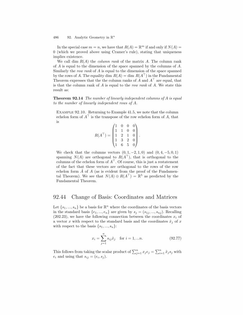
486 92. Analytic Geometry in Rn
In the special casem = n, we have that R(A) = Rm if and only ifN(A) =0 (which we proved above using Cramer’s rule), stating that uniquenessimplies existence.We call dim R(A) the column rank of the matrix A. The column rank
of A is equal to the dimension of the space spanned by the columns of A.Similarly the row rank of A is equal to the dimension of the space spannedby the rows of A. The equality dim R(A) = dim R(A⊤) in the FundamentalTheorem expresses that the the column ranks of A and A⊤ are equal, thatis that the column rank of A is equal to the row rank of A. We state thisresult as:
Theorem 92.14 The number of linearly independent columns of A is equalto the number of linearly independent rows of A.
Example 92.10. Returning to Example 41.5, we note that the columnechelon form of A⊤ is the transpose of the row echelon form of A, thatis
R(A⊤) =
1 0 0 01 1 0 01 2 1 01 3 2 01 6 5 0
.
We check that the columns vectors (0, 1,−2, 1, 0) and (0, 4,−5, 0, 1)spanning N(A) are orthogonal to R(A⊤), that is orthogonal to thecolumns of the echelon form of A⊤. Of course, this is just a restatementof the fact that these vectors are orthogonal to the rows of the rowechelon form A of A (as is evident from the proof of the Fundamen-tal Theorem). We see that N(A) ⊕ R(A⊤) = R5 as predicted by theFundamental Theorem.
92.44 Change of Basis: Coordinates and Matrices
Let s1, ..., sn be a basis for Rn where the coordinates of the basis vectorsin the standard basis e1, ..., en are given by sj = (s1j , ..., snj). Recalling(202.23), we have the following connection between the coordinates xi ofa vector x with respect to the standard basis and the coordinates xj of xwith respect to the basis s1, ..., sn:
xi =n∑
j=1
sij xj for i = 1, ...n. (92.77)
This follows from taking the scalar product of∑n
j=1 xjej =∑n
i=1 xjsj withei and using that sij = (ei, sj).

92.45 Least Squares Methods 487
Introducing the matrix S = (sij), we thus have the following connectionbetween the coordinates x = (x1, ..., xn) with respect to e1, ..., en, andthe coordinates x = (x1, ...xn) with respect to s1, ..., sn:
x = Sx, that is x = S−1x. (92.78)
Consider now a linear transformation f : Rn → Rn with matrix A = (aij)with respect to the standard basis e1, ...en, that is with aij = fi(ej) =(ei, f(ej)), where f(x) = (f1(x), ..., fn(x)) in the standard basis e1, ...en,that is
y = f(x) =∑i
fi(x)ei =n∑
i=1
n∑j=1
aijxjei = Ax.
Writing y = Sy and x = Sx, we have
Sy = ASx that is y = S−1ASx
This shows that the matrix of the linear transformation f : Rn → Rn, withthe matrix A with respect to the standard basis, takes the following formin the basis s1, ...sn:
S−1AS, (92.79)
where the the coefficients sij of the matrix S = (sij) are the coordinates ofthe basis vectors sj with respect to the standard basis.
92.45 Least Squares Methods
Consider the m× n linear system of equations Ax = b, or
n∑j
ajxj = b,
where A = (aij) is an m × n matrix with columns aj = (a1j , ..., amj),j = 1, ..., n. We know that if b ∈ R(A) then the system can be solved,and if N(A) = 0, then the solution is unique. Suppose now that b /∈ R(A).Then there is no x ∈ Rn such that Ax = b, and the system Ax = b has nosolution. We can replace the problem by the following least squares problem
minx∈Rn
|Ax− b|2.
This problem amounts to seeking the projection Pb of b onto R(A), that isthe projection of b onto the space spanned by the columns aj of A.By the properties of projections given above, we know that Pb ∈ R(A)
exists and is uniquely determined by the relation
(Pb, y) = (b, y) for all y ∈ R(A),

488 92. Analytic Geometry in Rn
that is we seek Pb = Ax for some x ∈ Rn such that
(Ax,Ax) = (b, Ax) for all x ∈ Rn.
This relation can be written
(A⊤Ax, x) = (A⊤b, x) for all x ∈ Rn,
which is the same as the matrix equation
A⊤Ax = A⊤b,
which we refer to as the normal equations.The matrix A⊤A is an n × n symmetric matrix. Assume now that the
columns aj of A are linearly independent. Then A⊤A is non-singular, be-cause if A⊤Ax = 0, then
0 = (A⊤Ax, x) = (Ax,Ax) = |Ax|2,
and thus Ax = 0 and therefore x = 0, since the columns of A are linearlyindependent. Thus the equation A⊤Ax = A⊤b has a unique solution x foreach right hand side A⊤b, given by the formula
x = (A⊤A)−1A⊤b.
In particular, we have the following formula for the projection Pb of b ontoR(A),
Pb = A(A⊤A)−1A⊤b.
We can directly check that P : Rm → Rm defined this way is symmetricand satisfies P 2 = P .If the columns of A are linearly dependent, then x is undetermined
up to vectors x in N(A). It is then natural to single out a unique x byrequiring that |x|2 to be minimal. Using the orthogonal decompositionRn = R(A⊤) ⊕ N(A), this is equivalent to seeking x in R(A⊤), since byPythagoras theorem this minimizes |x|. We thus seek x so that
• Ax is equal to the projection Pb of b onto R(A)
• x ∈ R(A⊤).
This leads to the following equation for x = A⊤y:
(Ax,AA⊤y) = (b, AA⊤y) for all y ∈ Rm, (92.80)
with x uniquely determined.
92.45 Least Squares Methods 489
Chapter 92 Problems
92.1. Prove that a plane in R3 not passing through the origin is not a subspaceof R3.
92.2. (a) What is a vector space? (b) What is a subspace of a vector space?
92.3. Verify (202.17) and (202.18).
92.4. Why must a set of more than n vectors in Rn be linearly dependent? Whymust a set of n linearly independent vectors in Rn be a basis?
92.5. Verify that R(A) and N(A) are linear subspaces of Rm and Rn, respec-tively, and further that the orthogonal complement V ⊤ of a subspace V of Rn isalso a subspace of Rn.
92.6. (a) Give an example showing that permutations need not commute. (b)Verify the associative law for permutations.
92.7. Compute the determinants of some n× n matrices with n = 2, 3, 4, 5.
92.8. Fill out the details in the proof of Cauchys inequality.
92.9. Write an algorithm for the Gram-Schmidt orthogonalization procedure,and implement it in Matlab, for example.
92.10. Fill in the details in (202.55)
92.11. Verify that for an orthogonal matrix QQ⊤ = I. Hint: Multiply Q⊤Q = Ifrom the right with C and from the right with Q, where C is the matrix suchthat QC = I.
92.12. Prove for 2× 2 matrices A and B that detAB = detA detB.
92.13. How many operations are needed to solve an n × n system of linearequations using Cramer’s formula?
92.14. Prove by reduction to column echelon form that a basis for Rn containsn elements.
92.15. Implement algorithms for reduction to column and row echelon forms.
92.16. Prove that the solution x ∈ R(A⊤) of (202.80) is uniquely determined.
92.17. Construct the row and column echelon forms of different (small) matrices,and check the validity of the Fundamental Theorem.

This is page 490Printer: Opaque this

This is page 491Printer: Opaque this
93The Spectral Theorem
There seems to be three possibilities (of a Unified Theory of Physics):
1. There really is a complete unified theory, which we will somedaydiscover if we are smart enough.
2. There is no ultimate theory of the Universe, just an infinitesequence of theories that describe the Universe more and moreaccurately.
3. There is no theory of the Universe; events cannot be predictedbeyond a certain extent but occur in a random and arbitrarymanner. (Stephen Hawking, in A Brief History of Time)
93.1 Eigenvalues and Eigenvectors
Let A = (aij) be a quadratic n× n matrix. We investigate the situation inwhich multiplication by A acts like scalar multiplication. To start with, weassume that the elements aij are real numbers. If x = (x1, ..., xn) ∈ Rn isa non-zero vector that satisfies
Ax = λx, (93.1)
where λ is a real number, then we say that x ∈ Rn is an eigenvector of Aand that λ is a corresponding eigenvalue of A. An eigenvector x has theproperty that Ax is parallel to x (if λ = 0), or Ax = 0 (if λ = 0). This is aspecial property, as easy to verify with almost any example we might makeup.

492 93. The Spectral Theorem
If x is an eigenvector with corresponding eigenvalue λ then x = µx forany non-zero real number µ is also an eigenvector corresponding to theeigenvalue λ because
if Ax = λx, then Ax = µAx = µλx = λµx = λx.
Thus, we may change the length of an eigenvector without changing thecorresponding eigenvalue. For example, we may normalize an eigenvectorto have length equal to 1. In essence, the direction of an eigenvector isdetermined, but not its length.We shall now study the problem of finding eigenvalues and corresponding
eigenvectors of a given a quadratic matrix. We shall see that this is a basicproblem of linear algebra arising in many different situations. We shallprove the Spectral Theorem stating that if A is a symmetric real n × nmatrix, then there is an orthogonal basis for Rn consisting of eigenvectors.We shall also briefly discuss the case of non-symmetric matrices.Rewriting (203.1) as (A− λI)x = 0 with x ∈ Rn a non-zero eigenvector
and I the identity matrix, we see that the matrixA−λI must be singular if λis an eigenvalue, that is det(A−λI) = 0. Conversely, if det(A−λI) = 0 thenA− λI is singular and thus the null-space N(A− λI) is different from thezero vector and thus there is a non-zero vector x such that (A− λI)x = 0,that is there is an eigenvector x with corresponding eigenvalue λ. Usingthe expansion formula for the determinant, we see that det(A − λI) is apolynomial in λ of degree n with coefficients depending on the coefficientsaij of A. The polynomial equation
det(A− λI) = 0
is called the characteristic equation. We summarize:
Theorem 93.1 The number λ is an eigenvalue of the n × n matrix A ifand only if λ is a root of the characteristic equation det(A− λI) = 0.
Example 93.1.
If A = (aij) is a 2× 2 matrix, then the characteristic equation is
det(A− λI) = (a11 − λ)(a22 − λ)− a12a21 = 0,
which is a second order polynomial equation in λ. For example, if
A =
(0 11 0
),
then the characteristic equation is det(A−λI) = λ2 − 1 = 0 with rootsλ1 = 1 and λ2 = −1. The corresponding normalized eigenvectors ares1 = 1√
2(1, 1) and s2 = 1√
2(1,−1) since
(A− λ1I)
(11
)=
(−1 11 −1
)(11
)=
(00
),

93.2 Basis of Eigenvectors 493
and similarly (A−λ2)s2 = 0. We observe that (s1, s2) = s1 ·s2 = 0, thatis eigenvectors corresponding to different eigenvalues are orthogonal.
93.2 Basis of Eigenvectors
Suppose s1, ..., sn is a basis for Rn consisting of eigenvectors of the n×nmatrix A = (aij) with corresponding eigenvalues λ1,...,λn so
Asi = λisi for i = 1, ..., n. (93.2)
Let S be the matrix with the columns equal to the eigenvectors sj expressedin the standard basis. We can then write (203.2) in matrix form as follows,
AS = SD, (93.3)
where D is the diagonal matrix with the eigenvalues λj on the diagonal.We thus have
A = SDS−1 or D = S−1AS, (93.4)
where D is a diagonal matrix. We say that S transforms A into a diagonalmatrix D with the eigenvalues on the diagonal.Conversely, if we can express a matrix A in the form A = SDS−1 with S
non-singular and D diagonal then AS = SD, which says that the columnsof S are eigenvectors with corresponding eigenvalues on the diagonal of D.Viewing the n × n matrix A as defining a linear transformation f :
Rn → Rn by f(x) = Ax, we can express the action of f(x) in a basisof eigenvectors s1, ..., sn by the diagonal matrix D since f(si) = λisi.Thus, the linear transformation f : Rn → Rn is expressed by the matrixA in the standard basis and by the diagonal matrix D matrix in a basis ofeigenvectors. The coupling is given by
D = S−1AS.
Of course, the action of a diagonal matrix is very easy to describe andto understand and this is the motivation for considering eigenvalues andeigenvectors.We now formulate the following basic question in two equivalent forms:
• Given a n× n matrix A, is there a basis of eigenvectors of A?
• Given a n × n matrix A, is there a non-singular matrix S such thatS−1AS is diagonal?
As we have seen, the columns of the matrix S are the eigenvectors of Aand the diagonal elements are the eigenvalues.We shall now give the following partial answer: if A is an n×n symmetric
matrix, then there is an orthogonal basis for Rn consisting of eigenvectors.
494 93. The Spectral Theorem
This is the celebrated Spectral Theorem for symmetric matrices. Noticethe assumption that A is symmetric and that in this case the basis ofeigenvectors may be chosen to be orthogonal.
Example 93.2. Recalling Example 203.1, we see that s1 = 1√2(1, 1)
and s2 = 1√2(1,−1) form an orthogonal basis. By the orthogonality of
S, S−1 = S⊤, and
S−1AS =1
2
(1 11 −1
)(0 11 0
)(1 11 −1
)=
1
2
(1 1−1 1
)(1 11 −1
)=
(1 00 −1
).
93.3 An Easy Spectral Theorem for SymmetricMatrices
The following version of the Spectral Theorem for symmetric matrices iseasy to prove:
Theorem 93.2 Let A be a symmetric n × n matrix. Suppose A has ndistinct eigenvalues λ1,..., λn and corresponding normalized eigenvectorss1,....,sn with ∥sj∥ = 1, j = 1, ..., n. Then, s1, ..., sn is an orthonormalbasis of eigenvectors. Letting Q = (qij) be the orthogonal matrix with thecolumns (q1j , ..., qnj) being the coordinates of the eigenvectors sj with re-spect to the standard basis, then D = Q−1AQ is a diagonal matrix with theeigenvalues λj on the diagonal and A = QDQ−1, where Q−1 = Q⊤.
To prove this result, it suffices to prove that eigenvectors correspondingto different eigenvalues are orthogonal. This follows from the assumptionthat there are n distinct eigenvalues λ1,..., λn with corresponding normal-ized eigenvectors s1,....,sn. If we prove that these eigenvectors are pairwiseorthogonal, then they form a basis for Rn and the proof is complete. Thus,assume that si and sj are eigenvectors corresponding to different eigenval-ues λi and λj . Since A is symmetric and (Ax, y) = (x,Ay) for all x, y ∈ Rn,we have
λi(si, sj) = (λisi, sj) = (Asi, sj) = (si, Asj)
= (si, λjsj) = λj(si, sj),
which implies that (si, sj) = 0 since λi = λj . We state this observation asa theorem because of its basic importance.
Theorem 93.3 If A is a symmetric n×n matrix, and si and sj are eigen-vectors of A corresponding to the eigenvalues λi and λj with λi = λj, then

93.4 Applying the Spectral Theorem to an IVP 495
(si, sj) = 0. In other words, eigenvectors corresponding to different eigen-values are orthogonal.
Note that above we prove the Spectral Theorem for a symmetric n × nmatrix A in the case the characteristic equation det(A − λI) = 0 has ndifferent roots. It thus remains to consider the case of multiple roots wherethere are less than n different roots. We will consider this below. The readerin hurry may skip that proof.
93.4 Applying the Spectral Theorem to an IVP
We show a typical application of the Spectral Theorem. Consider the initialvalue problem: find u : [0, 1] → Rn such that
u = Au, for 0 < t ≤ 1, u(0) = u0,
where A = (aij) is a symmetric n × n matrix with real coefficients aijindependent of t. Systems of this form arise in many applications and thebehavior of such a system may be very complicated.Suppose now that g1, ..., gn is an orthonormal basis of eigenvectors of
A and let Q be the matrix with columns comprised of the coordinates ofthe eigenvectors gj with respect to the standard basis. Then A = QDQ−1,where D is the diagonal matrix with the eigenvalues λj on the diagonal.We introduce the new variable v = Q−1u, that is we set u = Qv, wherev : [0, 1] → Rn. Then, the equation u = Au takes the form Qv = AQv, thatis v = Q−1AQv = Dv, where we use the fact that Q is independent of time.Summing up, we get the following diagonal system in the new variable v,
v = Dv for 0 < t ≤ 1, v(0) = v0 = Q−1u0.
The solution of this decoupled system is given by
v(t) =
exp(λ1t) 0 0 .... 0
0 exp(λ2t) 0 .... 0. . . . .0 0 0 .... exp(λn)
v0 = exp(Dt)v0,
where exp(Dt) is a diagonal matrix with the elements exp(λjt) on thediagonal. The dynamics of this system is easy to grasp: each componentvj(t) of v(t) evolves according to vj(t) = exp(λjt)v0j .Transforming back, we get the following solution formula in the original
variable u(t),
u(t) = Q exp(Dt)Q−1u0. (93.5)

496 93. The Spectral Theorem
With A as in Example 203.1, we get the solution formula
u(t) =1
2
(1 11 −1
)(et 00 e−t
)(1 11 −1
)(u01
u02
)=
1
2
((et + e−t)u01 + (et − e−t)u02
(et − e−t)u01 + (et + e−t)u02
).
93.5 The General Spectral Theorem for SymmetricMatrices
Above, we saw that eigenvalues of a matrix A are roots of the characteristicequation det(A − λI) = 0. In principle, we can find the eigenvalues andeigenvectors of given matrix by first solving the characteristic equation tofind all the eigenvalues, and then for each eigenvalue λ find correspondingeigenvectors by solving the linear system of equations (A− λI)x = 0.We shall now present an alternative way of constructing/finding the
eigenvectors and eigenvalues of a symmetric matrix A that also provesthe Spectral Theorem for a symmetric n× n matrix A in the general casewith possibly multiple roots. In the proof, we construct an orthonormalbasis of eigenvectors s1, ..., sn of A by constructing the eigenvectors oneby one starting with s1.
Constructing the First Eigenvector s1
To construct the first eigenvector s1, we consider the minimization problem:find x ∈ Rn such that
F (x) = minx∈Rn
F (x), (93.6)
where
F (x) =(Ax, x)
(x, x)=
(f(x), x)
(x, x)(93.7)
is the so-called Rayleigh quotient. We note that the function F (x) is ho-mogenous of degree zero, that is for any λ ∈ R, λ = 0, we have
F (x) = F (λx),
because we can simply divide out the factor λ. In particular, for any x = 0,
F (x) = F (x
∥x∥), (93.8)
and thus we may restrict the x in (203.6) to have length one, that is wemay consider the equivalent minimization problem: find x with ∥x∥ = 1such that
F (x) = minx∈Rn ∥x∥=1
F (x) (93.9)

93.5 The General Spectral Theorem for Symmetric Matrices 497
Since F (x) is Lipschitz continuous on the closed and bounded subset x ∈Rn : ∥x∥ = 1 of Rn, we know by the Chapter Minimization, that theproblem (203.9) has a solution x, and thus also the problem (203.6) has asolution x. We set s1 = x, and check that g1 is indeed an eigenvector of A,that is an eigenvector of f : Rn → Rn.Since x solves the minimization problem (203.6), we have ∇F (x) = 0,
where ∇F is the gradient of F . Computing ∇F (x) using the symmetry ofF (x) or the matrix A, we find that
∇F (x) =(x, x)2Ax− (Ax, x)2x
(x, x)2, (93.10)
so that with x = x satisfying (x, x) = 1,
∇F (x) = 2(Ax− (Ax, x)x) = 0,
that isAx = λ1x, (93.11)
where
λ1 = (Ax, x) =(Ax, x)
(x, x)= min
x∈RnF (x). (93.12)
Setting s1 = x, we thus have
As1 = λ1s1, λ1 = (As1, s1), ∥s1∥ = 1.
We have now constructed the first normalized eigenvector s1 with corre-sponding eigenvalue λ1. We now let V1 be the orthogonal complement ofthe space spanned by s1, consisting of all the vectors x ∈ Rn such that(x, s1) = 0. The dimension of V1 is n− 1.
Invariance of A
Note that V1 is invariant with respect to A in the sense that if x ∈ V1 thenAx ∈ V1. This follows because if (x, g1) = 0 then (Ax, s1) = (x,As1) =(x, λ1s1) = λ1(x, s1) = 0. This means that we can now restrict attention tothe action of A on V1, having handled the action of A on the space spannedby the first eigenvector s1.
Constructing the Second Eigenvector s2
Consider the minimization problem to find x ∈ V1 such that
F (x) = minx∈V1
F (x). (93.13)
By the same argument, this problem has a solution which we denote s2 and
which satisfies As2 = λ2s2, where λ2 = (As2,s2)(s2,s2)
, and ∥s2∥ = 1. Because in

498 93. The Spectral Theorem
(203.13) we minimize over a smaller set than in (203.6), λ2 ≥ λ1. Note thatit may happen that λ2 = λ1, although V1 is a subset of Rn. In that case,we say that λ1 = λ2 is a multiple eigenvalue.
Continuing the Process
Let V2 be the orthogonal subspace to the space spanned by s1 and s2Again A is invariant on V2 and the space spanned by s1, s2. Continuingthis way, we obtain a orthonormal basis s1, ..., sn of eigenvectors of Awith corresponding real eigenvalues λi.We have now proved the famous
Theorem 93.4 (Spectral Theorem): If f : R → R is a linear sym-metric transformation with corresponding symmetric n × n matrix A inthe standard basis, then there is an orthogonal basis (g1, ..., gn) of Rn con-sisting of eigenvectors gi of f with corresponding real eigenvalues λj sat-isfying f(gj) = Agj = λjgj, for j = 1, ..., n. We have D = Q−1AQ andA = QDQ−1, where Q is the orthogonal matrix with the coefficients of theeigenvectors gj in the standard basis forming the columns, and D is thediagonal matrix with the eigenvalues λj on the diagonal.
93.6 The Norm of a Symmetric Matrix
We recall that we have defined the Euclidean norm ∥A∥ of a n× n matrixA by
∥A∥ = maxx∈Rn
∥Ax∥∥x∥
, (93.14)
where we maximize over x = 0. By the definition, we have
∥Ax∥ ≤ ∥A∥ ∥x∥, (93.15)
and we may thus view ∥A∥ to be the smallest constant C such that ∥Ax∥ ≤C∥x∥ for all x ∈ Rn.We shall now prove that if A is symmetric, then we can directly relate
∥A∥ to the eigenvalues λ1, ..., λn of A:
∥A∥ = maxi=1,...,n
|λi|. (93.16)
We do this as follows. Using the Spectral theorem, we can write A as A =Q⊤ΛQ with Q orthogonal and Λ a diagonal matrix with the eigenvalues λi
on the diagonal. We recall that (cf. (202.46))
∥Λ∥ = maxi=1,...,n
|λi| = |λj | (93.17)

93.7 Extension to Non-Symmetric Real Matrices 499
and thus for all x ∈ Rn,
∥Ax∥ = ∥Q⊤ΛQx∥ = ∥ΛQx∥ ≤ ∥Λ∥∥Qx∥ = ∥Λ∥∥x∥ = maxi=1,...,n
|λi|∥x∥,
which proves that ∥A∥ ≤ maxi=1,...,n |λi|. Choosing x to be equal to theeigenvector corresponding to the eigenvalue λj of maximal modulus provesthat indeed ∥A∥ = maxi=1,...,n |λi| = |λj |. We have proved the followingresult, which is a corner stone of numerical linear algebra.
Theorem 93.5 If A is a symmetric n × n matrix, then ∥A∥ = max |λi|,where λ1, ..., λn are the eigenvalues of A.
93.7 Extension to Non-Symmetric Real Matrices
Up until now, we have mainly focussed on the case of real scalars, thatis we assume that the components of vectors are real numbers. We knowthat we can also let the components of vectors be complex numbers, andwe may then allow eigenvalues to be complex numbers. The fundamentaltheorem of algebra states that a polynomial equation of degree n with com-plex coefficients, has n complex roots, and thus the characteristic equationdet(A− λI) = 0 has n complex roots λ1,....,λn, and thus a n× n matrix Ahas n complex eigenvalues λ1,....,λn, if roots are counted with multiplicity.We have in this chapter focussed on symmetric matrices A with real coef-ficients and we have proved that a symmetric matrix with real coefficientshas n real eigenvalues, counted with multiplicity. For symmetric matriceswe can thus limit ourselves to real roots of the characteristic equation.
Chapter 93 Problems
93.1. Verify (203.10).
93.2. Compute the eigenvalues and eigenvectors of an arbitrary symmetric 2×2matrix A. Solve the corresponding initial-value problem u(t) = Au(t) for t > 0,u(0) = u0.

This is page 500Printer: Opaque this
This is page 501Printer: Opaque this
94Solving Linear Algebraic Systems
All thought is a kind of computation. (Hobbes)
94.1 Introduction
We are interested in solving a system of linear equations
Ax = b,
where A is a given n × n matrix and b ∈ Rn is a given n-vector and weseek the solution vector x ∈ Rn. We recall that if A is non-singular withnon-zero determinant, then the solution x ∈ Rn is theoretically given byCramer’s formula. However if n is large, the computational work in usingCramer’s formula is prohibitively large, so we need to find a more efficientmeans of computing the solution.We shall consider two types of methods for solving the system Ax = b: (i)
direct methods based on Gaussian elimination that theoretically producea solution after a finite number of arithmetic operations, and (ii) iterativemethods that produce a generally infinite sequence of increasingly accurateapproximations.
94.2 Direct Methods
We begin by noting that some linear systems are easier to solve than others.For example if A = (aij) is diagonal, which means that aij = 0 if i = j,

502 94. Solving Linear Algebraic Systems
then the system is solved in n operations: xi = bi/aii, i = 1, ..., n. Further,if the matrix is upper triangular, which means that aij = 0 if i > j, orlower triangular, which means that aij = 0 if i < j, then the system canbe solved by backward substitution or forward substitution respectively; seeFig. 253.4 for an illustration of these different types. For example if A is
0
0 0
0
FIGURE 94.1. The pattern of entries in diagonal, upper, and lower triangularmatrices. A “∗” denotes a possibly nonzero entry.
upper triangular, the “pseudo-code” shown in Fig. 253.5 solves the systemAx = b for the vector x = (xi) given the vector b = (bi) (assuming thatakk = 0): In all three cases, the systems have a unique solution as long as
for k = n-1, n-2, ..., 1, do
sum = 0
for j = k+1, ..., n, do
sum = sum + akj. xj
xk = (bk - sum)/akk
xn = bn/ann
FIGURE 94.2. An algorithm for solving an upper triangular system by backsubstitution.
the diagonal entries of A are nonzero.Direct methods are based on Gaussian elimination, which in turn is based
on the observation that the solution of a linear system is not changed underthe following elementary row operations:
• interchanging two equations
• adding a multiple of one equation to another
• multiplying an equation by a nonzero constant.
The idea behind Gaussian elimination is to transform using these opera-tions a given system into an upper triangular system, which is solved by
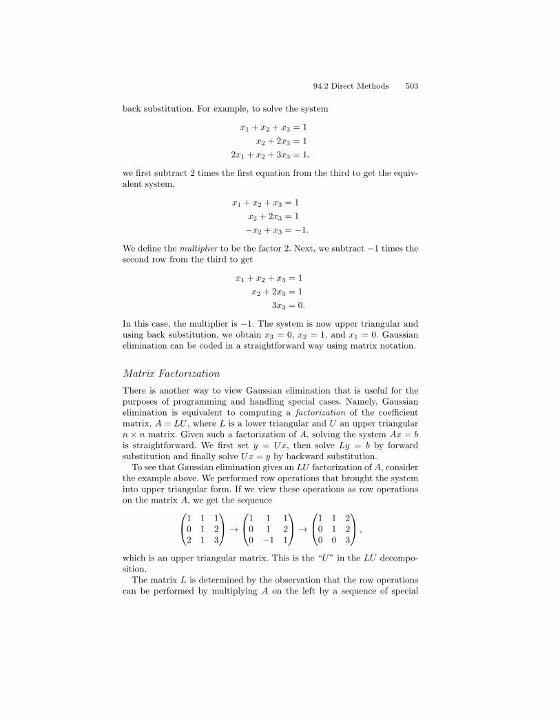
94.2 Direct Methods 503
back substitution. For example, to solve the system
x1 + x2 + x3 = 1
x2 + 2x3 = 1
2x1 + x2 + 3x3 = 1,
we first subtract 2 times the first equation from the third to get the equiv-alent system,
x1 + x2 + x3 = 1
x2 + 2x3 = 1
−x2 + x3 = −1.
We define the multiplier to be the factor 2. Next, we subtract −1 times thesecond row from the third to get
x1 + x2 + x3 = 1
x2 + 2x3 = 1
3x3 = 0.
In this case, the multiplier is −1. The system is now upper triangular andusing back substitution, we obtain x3 = 0, x2 = 1, and x1 = 0. Gaussianelimination can be coded in a straightforward way using matrix notation.
Matrix Factorization
There is another way to view Gaussian elimination that is useful for thepurposes of programming and handling special cases. Namely, Gaussianelimination is equivalent to computing a factorization of the coefficientmatrix, A = LU , where L is a lower triangular and U an upper triangularn × n matrix. Given such a factorization of A, solving the system Ax = bis straightforward. We first set y = Ux, then solve Ly = b by forwardsubstitution and finally solve Ux = y by backward substitution.To see that Gaussian elimination gives an LU factorization of A, consider
the example above. We performed row operations that brought the systeminto upper triangular form. If we view these operations as row operationson the matrix A, we get the sequence1 1 1
0 1 22 1 3
→
1 1 10 1 20 −1 1
→
1 1 20 1 20 0 3
,
which is an upper triangular matrix. This is the “U” in the LU decompo-sition.The matrix L is determined by the observation that the row operations
can be performed by multiplying A on the left by a sequence of special

504 94. Solving Linear Algebraic Systems
matrices called Gauss transformations. These are lower triangular matri-ces that have at most one nonzero entry in the off-diagonal positions and1s down the diagonal. We show a Gauss transformation in Fig. 253.6.Multiplying A on the left by the matrix in Fig. 253.6 has the effect of
1 0 · · · 00 1 0 0
. . . 1. . . 0
......
0 0 0. . . 0
0 αij 0. . . 1
. . .
0 0 0. . .
0 1 00 · · · 0 1
FIGURE 94.3. A Gauss transformation.
adding αij times row j of A to row i of A. Note that the inverse of thismatrix is obtained changing αij to −αij ; we will use this below.To perform the first row operation on A above, we multiply A on the left
by
L1 =
1 0 00 1 0−2 0 1
,
to get
L1A =
1 1 10 1 20 −1 −1
.
The effect of pre-multiplication by L1 is to add −2× row 1 of A to row 3.Note that L1 is lower triangular and has ones on the diagonal.Next we multiply L1A on the left by
L2 =
1 0 00 1 00 1 1
,
and get
L2L1A =
1 1 10 1 20 0 3
= U.

94.2 Direct Methods 505
L2 is also lower triangular with ones on the diagonal. It follows that A =L−11 L−1
2 U or A = LU , where
L = L−11 L−1
2 =
1 0 00 1 02 −1 1
.
It is easy to see that L is also lower triangular with 1’s on the diagonal withthe multipliers (with sign change) occurring at the corresponding positions.We thus get the factorization
A = LU =
1 0 00 1 02 −1 1
1 1 10 1 20 0 3
.
Note that the entries in L below the diagonal are exactly the multipliersused to perform Gaussian elimination on A.A general linear system can be solved in exactly the same fashion by
Gaussian elimination using a sequence of Gauss transformations to obtaina factorization A = LU .An LU factorization can be performed in situ using the storage space
allotted to the matrix A. The fragment of code shown in Fig. 253.7 com-putes the LU factorization of A, storing U in the upper triangular part ofA and storing the entries in L below the diagonal in the part of A belowthe diagonal. We illustrate the storage of L and U in Fig. 253.8.
for k = 1, ..., n-1, do
for j = k+1, ..., n, do
ajk = ajk/akk
for m = k+1, ..., n, do
ajm = ajm - ajk akm
(step through rows)
(store the entry of L)
(eliminate entriesbelow diagonal entry)
(correct entriesdown the row)
(store the entry of U)
FIGURE 94.4. An algorithm to compute the LU factorization of A that storesthe entries of L and U in the storage space of A.
Measuring the Cost
The cost of solving a linear system using a direct method is measuredin terms of computer time. In practice, the amount of computer time is

506 94. Solving Linear Algebraic Systems
u11
u22
unn
u12 u1n
l21
ln1 lnn-1
FIGURE 94.5. The matrix output from the algorithm in Fig. 253.7. L and U arestored in the space allotted to A.
proportional to the number of arithmetic and storage operations the com-puter uses to compute the solution. It is traditional (on a sequential com-puter) to simplify the cost calculation by equating storing a value, addition,and subtraction and equating multiplication and division when countingoperations. Moreover, since multiplication (i.e. multiplications and divi-sions) generally cost much more than addition on older computers, it isalso common to simply count the number of multiplications (=multiplica-tions+divisions).By this measure, the cost of computing the LU decomposition of an n×n
matrix is n3 − n/3 = O(n3/3). We introduce some new notation here, thebig “O”. The actual count is n3/3−n/3, however when n is large, the lowerorder term −n/3 becomes less significant. In fact,
limn→∞
n3/3− n/3
n3/3= 1, (94.1)
and this is the definition of the big “O”. (Sometimes the big “O” notationmeans that the limit of the ratio of the two relevant quantities is any con-stant). With this notation, the operations count of the LU decompositionis just O(n3).The cost of the forward and backward substitutions is much smaller:
Pivoting
During Gaussian elimination, it sometimes happens that the coefficient ofa variable in the “diagonal position” becomes zero as a result of previouseliminations. When this happens of course, it is not possible to use thatequation to eliminate the corresponding entries in the same column lyingbelow the diagonal position. If the matrix is invertible, it is possible to finda non-zero coefficient in the same column and below the diagonal position,and by switching the two rows, the Gaussian elimination can proceed. Thisis called zero pivoting, or just pivoting.Adding pivoting to the LU decomposition algorithm is straightforward.
Before beginning the elimination using the current diagonal entry, we check
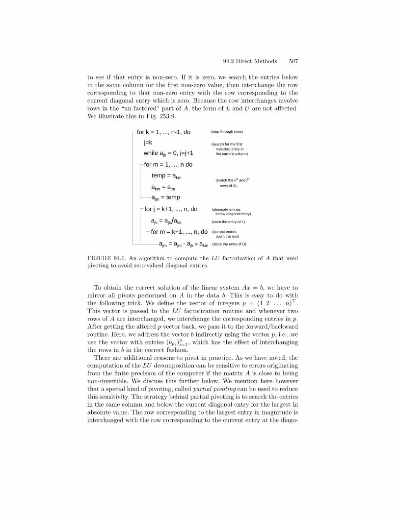
94.2 Direct Methods 507
to see if that entry is non-zero. If it is zero, we search the entries belowin the same column for the first non-zero value, then interchange the rowcorresponding to that non-zero entry with the row corresponding to thecurrent diagonal entry which is zero. Because the row interchanges involverows in the “un-factored” part of A, the form of L and U are not affected.We illustrate this in Fig. 253.9.
for k = 1, ..., n-1, do
for j = k+1, ..., n, do
ajk = ajk/akk
for m = k+1, ..., n, do
ajm = ajm - ajk akm
(step through rows)
(store the entry of L)
(eliminate entriesbelow diagonal entry)
(correct entriesdown the row)
(store the entry of U)
j=k
while ajk = 0, j=j+1
for m = 1, ..., n do
temp = akm
akm = ajm
ajm = temp
(search for the firstnon-zero entry inthe current column)
(switch the kth and jth
rows of A)
FIGURE 94.6. An algorithm to compute the LU factorization of A that usedpivoting to avoid zero-valued diagonal entries.
To obtain the correct solution of the linear system Ax = b, we have tomirror all pivots performed on A in the data b. This is easy to do withthe following trick. We define the vector of integers p = (1 2 . . . n)⊤.This vector is passed to the LU factorization routine and whenever tworows of A are interchanged, we interchange the corresponding entries in p.After getting the altered p vector back, we pass it to the forward/backwardroutine. Here, we address the vector b indirectly using the vector p, i.e., weuse the vector with entries (bpi)
ni=1, which has the effect of interchanging
the rows in b in the correct fashion.There are additional reasons to pivot in practice. As we have noted, the
computation of the LU decomposition can be sensitive to errors originatingfrom the finite precision of the computer if the matrix A is close to beingnon-invertible. We discuss this further below. We mention here howeverthat a special kind of pivoting, called partial pivoting can be used to reducethis sensitivity. The strategy behind partial pivoting is to search the entriesin the same column and below the current diagonal entry for the largest inabsolute value. The row corresponding to the largest entry in magnitude isinterchanged with the row corresponding to the current entry at the diago-

508 94. Solving Linear Algebraic Systems
nal. The use of partial pivoting generally gives more accurate results thanfactorization without partial pivoting. One reason is that partial pivotinginsures that the multipliers in the elimination process are kept as small aspossible and consequently the errors in each entry are magnified by as littleas possible during the course of the Gaussian elimination. We illustrate thiswith an example. Suppose that we solve
.000100x1 + 1.00x2 = 1.00
1.00x1 + 1.00x2 = 2.00
on a computer that holds three digits. Without pivoting, we get
.000100x1 + 1.00x2 = 1.00
−10000x2 = −10000
which implies that x2 = 1 and x1 = 0. Note the large multiplier that isrequired for the elimination. Since the true answer is x1 = 1.0001 andx2 = .9999, the computed result has an error of 100% in x1. If we switchthe two rows before eliminating, which corresponds exactly to the partialpivoting strategy, we get
1.00x1 + 1.00x2 = 2.00
1.00x2 = 1.00
which gives x1 = x2 = 1.00 as a result.
94.3 Direct Methods for Special Systems
It is often the case that the matrices arising from the Galerkin finite elementmethod applied to a differential equation have special properties that canbe useful during the solution of the associated algebraic equations. Forexample, the stiffness matrix for the Galerkin finite element approximationof the two-point boundary value problem with no convection is symmetric,positive-definite, and tridiagonal. In this section, we examine a couple ofdifferent classes of problems that occur frequently.
Symmetric, Positive-Definite Systems
As we mentioned, symmetric, positive-definite matrices are often encoun-tered when discretizing differential equations (especially if the spatial partof the differential equation is of the type called elliptic). If A is symmetricand positive-definite, then it can be factored as A = BB⊤ where B is alower triangular matrix with positive diagonal entries. This factorizationcan be computed from the LU decomposition of A, but there is a compact

94.3 Direct Methods for Special Systems 509
method of factoring A that requires only O(n3/6) multiplications calledCholesky’s method.:
b11 =√a11
bi1 =ai1b11
, 2 ≤ i ≤ n,bjj =(ajj −
∑j−1k=1 b
2jk
)1/2,
bij =(aij −
∑j−1k=1 bikbjk
)/bjj ,
2 ≤ j ≤ n, j + 1 ≤ i ≤ n
This is called a compact method because it is derived by assuming thatthe factorization exists and then computing the coefficients of B directlyfrom the equations obtained by matching coefficients in BB⊤ = A. Forexample, if we compute the coefficient in the first row and column of BB⊤
we get b211, which therefore must equal a11. It is possible to do this becauseA is positive-definite and symmetric, which implies among other thingsthat the diagonal entries of A remain positive throughout the factorizationprocess and pivoting is not required when computing an LU decomposition.Alternatively, the square roots in this formula can be avoided by com-
puting a factorization A = CDC⊤ where C is a lower triangular matrixwith ones on the diagonal and D is a diagonal matrix with positive diagonalcoefficients.
Banded Systems
Banded systems are matrices with non-zero coefficients only in some num-ber of diagonals centered around the main diagonal. In other words, aij = 0for j ≤ i− dl and j ≥ i+ du, 1 ≤ i, j ≤ n, where dl is the lower bandwidth,du is the upper bandwidth, and d = du+dl−1 is called the bandwidth. We il-lustrate this in Fig. 253.10. The stiffness matrix computed for the two-pointboundary value problem with no convection is an example of a tridiagonalmatrix, which is a matrix with lower bandwidth 2, upper bandwidth 2, andbandwidth 3.When performing the Gaussian elimination used to compute the LU
decomposition, we see that the entries of A that are already zero do nothave to be reduced further. If there are only relatively few diagonals withnon-zero entries, then the potential saving is great. Moreover, there is noneed to store the zero-valued entries of A. It is straightforward to adapt theLU factorization and forward/backward substitution routines to a bandedpattern, once a storage scheme has been devised. For example, we can store

510 94. Solving Linear Algebraic Systems
a11
a22
ann
a12 0a21
0
a13 a1du0
adl1
0
ann-dl+10
ann-du+1
0
du
dl
FIGURE 94.7. The notation for a banded matrix.
a tridiagonal matrix as a 3× n matrix:
a21 a31 0 · · · 0a12 a22 a32 0 · · · 0
0 a13 a23 a33 0 · · ·...
. . .. . .
. . .. . .
. . . 0... 0 a1n−1 a2n−1 a3n−1
0 · · · 0 a1n a2n
.
The routine displayed in Fig. 253.11 computes the LU factorization, whilethe routine in Fig. 253.12 performs the forward/backward substitution.
for k = 2, ..., n, do
a1k = a1k/a2k-1
a2k = a2k - a1k a3k-1
FIGURE 94.8. A routine for computing the LU factorization of a tridiagonalsystem.
The cost of this routine grows linearly with the dimension, rather thanat a cubic rate as in the full case. Moreover, we use only the equivalent ofsix vectors of dimension n for storage. A more efficient version, derived asa compact method, uses even less.This algorithm assumes that no pivoting is required to factor A. Pivoting
during the factorization of a banded matrix raises the difficulty that the

94.4 Iterative Methods 511
for k = n-1, ..., 1, do
xn = yn/a2n
xk = yk - a3k xk+1 /a2k
for k = 2, ..., n, do
y1 = b1
yk = bk - a1k yk-1
FIGURE 94.9. Using forward and backward substitution to solve a tridiagonalsystem given the LU factorization.
bandwidth becomes larger. This is easy to see in a tridiagonal matrix, inwhich case we have to store an extra vector to hold the extra elementsabove the diagonal that result if two adjacent rows are switched.As for a tridiagonal matrix, it is straightforward to program special LU
factorization and forward/backward substitution routines for a matrix withbandwidth d. The operations count is O(nd2/2) and the storage require-ment is a matrix of dimension d× n if no pivoting is required. If d is muchless than n, the savings in a special approach are considerable.While it is true that if A is banded, then L and U are also banded,
it is also true that in general L and U have non-zero entries in positionswhere A is zero. This is called fill-in. In particular, the stiffness matrix for aboundary value problem in several variables is banded and moreover mostof the sub-diagonals in the band have zero coefficients. However, L and Udo not have this property and we may as well treat A as if all the diagonalsin the band have non-zero entries.Banded matrices are one example of the class of sparse matrices. Recall
that a sparse matrix is a matrix with mostly zero entries. As for bandedmatrices, it is possible to take advantage of sparsity to reduce the cost offactoring A in terms of time and storage. However, it is more difficult to dothis than for banded matrices if the sparsity pattern puts non-zero entriesat any location in the matrix. One approach to this problem is based onrearranging the equations and variables, or equivalently rearranging therows and columns to form a banded system.
94.4 Iterative Methods
Instead of solving Ax = b directly, we now consider iterative solution meth-ods based on computing a sequence of approximations x(k), k = 1, 2, ...,such that
limk→∞
x(k) = x or limk→∞
∥x(k) − x∥ = 0,
512 94. Solving Linear Algebraic Systems
for some norm ∥ · ∥.Note that the finite precision of a computer has a different effect on an
iterative method than it has on a direct method. A theoretically convergentsequence can not reach its limit in general on a computer using a finitenumber of digits. In fact, at the point at which the change from one iterateto the next occurs outside the range of digits held by the computer, thesequence simply stops changing. Practically speaking, there is no pointcomputing iterations past this point, even if the limit has not been reached.On the other hand, it is often sufficient to have less accuracy than the limitof machine precision, and thus it is important to be able to estimate theaccuracy of the current iterate.
Minimization Algorithms
We first construct iterative methods for a linear system Ax = b whereA is symmetric and positive-definite. In this case, the solution x can becharacterized equivalently as the solution of the quadratic minimizationproblem: find x ∈ Rn such that
F (x) ≤ F (y) for all y ∈ Rn, (94.2)
where
F (y) =1
2(Ay, y)− (b, y),
with (·, ·) denoting the usual Euclidean scalar product.We construct an iterative method for the solution of the minimization
problem (253.6) based on the following simple idea: given an approximationx(k), compute a new approximation x(k+1) such that F (x(k+1)) < F (x(k)).On one hand, since F is a quadratic function, there must be a “downhill”direction from the current position, unless we are at the minimum. Onthe other hand, we hope that computing the iterates so that their func-tion values are strictly decreasing, will force the sequence to converge tothe minimum point x. Such an iterative method is called a minimizationmethod.Writing x(k+1) = x(k) + αkd
(k), where d(k) is a search direction and αk
is a step length, by direct computation we get
F (x(k+1)) = F (x(k)) + αk
(Ax(k) − b, d(k)
)+
α2k
2
(Ad(k), d(k)
),
where we used the symmetry of A to write (Ax(k), d(k))=(x(k), Ad(k)). If thestep length is so small that the second order term in αk can be neglected,then the direction d(k) in which F decreases most rapidly, or the directionof steepest descent, is
d(k) = −(Ax(k) − b) = −r(k),
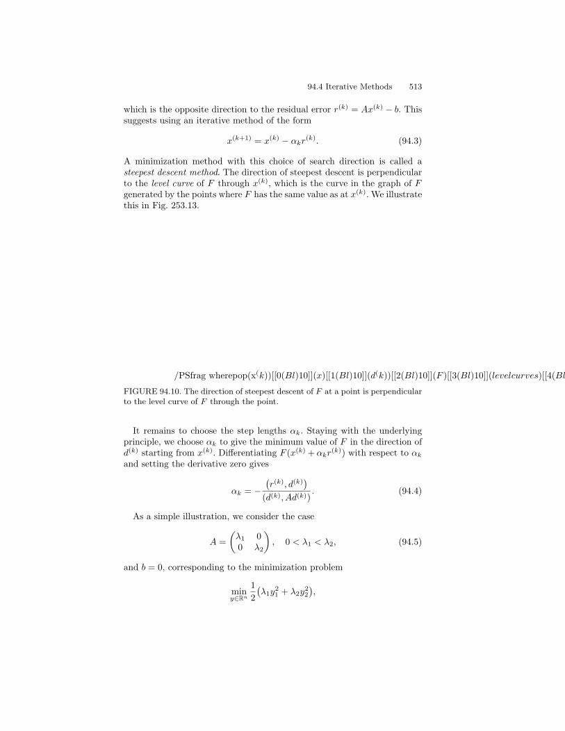
94.4 Iterative Methods 513
which is the opposite direction to the residual error r(k) = Ax(k) − b. Thissuggests using an iterative method of the form
x(k+1) = x(k) − αkr(k). (94.3)
A minimization method with this choice of search direction is called asteepest descent method. The direction of steepest descent is perpendicularto the level curve of F through x(k), which is the curve in the graph of Fgenerated by the points where F has the same value as at x(k). We illustratethis in Fig. 253.13.
/PSfrag wherepop(x(k))[[0(Bl)10]](x)[[1(Bl)10]](d(k))[[2(Bl)10]](F )[[3(Bl)10]](levelcurves)[[4(Bl)10]]501/BeginPSfraguserdict/PSfragpopputifelse
d^(k)x^(k)
level curves
F
xx^(k)
x
/EndPSfrag /Hide PSfragPSfrag replacements/Unhide PSfrag– x(k)˝ 0/Place PSfrag– x 1/Place PSfrag– d(k)˝ 2/Place PSfrag– F 3/Place PSfrag– level curves˝ 4/Place PSfrag
FIGURE 94.10. The direction of steepest descent of F at a point is perpendicularto the level curve of F through the point.
It remains to choose the step lengths αk. Staying with the underlyingprinciple, we choose αk to give the minimum value of F in the direction ofd(k) starting from x(k). Differentiating F (x(k) +αkr
(k)) with respect to αk
and setting the derivative zero gives
αk = −(r(k), d(k)
)(d(k), Ad(k))
. (94.4)
As a simple illustration, we consider the case
A =
(λ1 00 λ2
), 0 < λ1 < λ2, (94.5)
and b = 0, corresponding to the minimization problem
miny∈Rn
1
2
(λ1y
21 + λ2y
22
),

514 94. Solving Linear Algebraic Systems
with solution x = 0.Applying (253.7) to this problem, we iterate according to
x(k+1) = x(k) − αkAx(k),
using for simplicity a constant step length with αk = α instead of (253.8).In Fig. 253.14, we plot the iterations computed with λ1 = 1, λ2 = 9, andx(0) = (9, 1)⊤. The convergence in this case is quite slow. The reason is that
if λ2 ≫ λ1, then the search direction −(λ1x(k)1 , λ2x
(k)2 )⊤ and the direction
−(x(k)1 , x
(k)2 )⊤ to the solution at the origin, are very different. As a result
the iterates swing back and forth across the long, narrow “valley”.
/PSfrag wherepop(x1)[[0(Bl)10]](x2)[[1(Bl)10]](x(0))[[2(Bl)10]](x(1))[[3(Bl)10]](x(2))[[4(Bl)10]]501/BeginPSfraguserdict/PSfragpopputifelse
0 2 4 6 8
−1
−0.5
0.5
1
x_1
x_2
x^(0)
x^(1)
x^(2)
/EndPSfrag /Hide PSfragPSfrag replacements/Unhide PSfrag– x1 0/Place PSfrag– x2 1/Place PSfrag– x(0)˝ 2/Place PSfrag– x(1)˝ 3/Place PSfrag– x(2)˝ 4/Place PSfrag
FIGURE 94.11. A sequence generated by the steepest descent method for (253.9)plotted together with some level curves of F .
It turns out that the rate at which the steepest descent method convergesin general depends on the condition number κ(A) = λn/λ1 of A, whereλ1 ≤ λ2 ≤ ... ≤ λn are the eigenvalues of A (counted with multiplicity). Inother words, the condition number of a symmetric positive definite matrixis the ratio of the largest eigenvalue to the smallest eigenvalue.The general definition of the condition number of a matrix A in terms of
a norm ∥ · ∥ is κ(A) = ∥A∥∥A−1∥. In the ∥ · ∥2 norm, the two definitions areequivalent for symmetric matrices. Using any definition, a matrix is saidto be ill-conditioned if the log(κ(A)) is of the order of the number of digitsused in the computer. As we said, we can expect to have difficulty solvingan ill-conditioned system; which in terms of direct methods means largeerrors due to rounding errors and in terms of iterative methods means slowconvergence.
94.4 Iterative Methods 515
We now analyze the steepest descent method for Ax = b in the case of aconstant step length α, where we iterate according to
x(k+1) = x(k+1) − α(Ax(k) − b).
Since the exact solution x satisfies x = x−α(Ax− b), we get the followingequation for the error e(k) = x− x(k):
e(k+1) = (I − αA)e(k).
The iterative method converges if the error tend to zero. Taking norms, weget
∥e(k+1)∥ ≤ µ ∥e(k)∥ (94.6)
where we use the spectral estimate (203.16) to write
µ = ∥I − αA∥ = maxj
|1− αλj |,
since the eigenvalues of the matrix I−αA are 1−αλj , j = 1, ..., n. Iteratingthis estimate we get
∥e(k+1)∥ ≤ µk ∥e(0)∥, (94.7)
where e(0) is the initial error.To understand when (253.10), or (253.11), guarantees convergence, con-
sider the scalar sequence λk for k ≥ 0. If |λ| < 1, then λk → 0; if λ = 1,then the sequence is always 1; if λ = −1, the sequence alternates between 1and −1 and does not converge; and if |λ| > 1, then the sequence diverges.Therefore if we want the iteration to converge for any initial value, thenwe must choose α so that µ < 1. Since the λj are positive by assumption,1 − αλj < 1 automatically, and we can guarantee that 1 − αλj > −1 if αsatisfies α < 2/λn. Choosing α = 1/λn, which is not so far from optimal,we get
µ = 1− 1/κ(A).
If κ(A) is large, then the convergence can be slow because then thereduction factor 1− 1/κ(A) is close to one. More precisely, the number ofsteps required to lower the error by a given amount is proportional to thecondition number.When an iteration converges in this fashion, i.e. the error decreases (more
or less) by a given factor in each iteration, then we say that the iterationconverges linearly. We define the rate of convergence to be − log(µ). Themotivation is that the number of iterations are required to reduce the errorby a factor of 10−m is approximately −m log(µ). Note that a faster rate ofconvergence means a smaller value of µ.This is an a priori estimate of the error reduction per iteration, since we
estimate the error before the computation. Such an analysis must accountfor the slowest possible rate of convergence because it holds for all initialvectors.
516 94. Solving Linear Algebraic Systems
Consider the system Ax = 0 with
A =
λ1 0 00 λ2 00 0 λ3
, (94.8)
where 0 < λ1 < λ2 < λ3. For an initial guess x(0)=(x01, x
02, x
03)
⊤, thesteepest descent method with α = 1/λ3 gives the sequence
x(k) =
((1− λ1
λ3
)kx01,(1− λ2
λ3
)kx02, 0
), k = 1, 2, ...,
and,
∥e(k)∥ =
√(1− λ1
λ3
)2k (x01
)2+
(1− λ2
λ3
)2k (x02
)2, k = 1, 2, ...
Thus for a general initial guess, the size of the error is given by the rootmean square average of the corresponding iterate and the rate that theerrors decrease is the root mean square average of the rates of decrease ofthe components. Therefore, depending on the initial vector, initially theiterates will generally converge more quickly than the rate of decrease ofthe first, i.e. slowest, component. In other words, more quickly than therate predicted by (253.10), which bounds the rate of decrease of the errorsby the rate of decrease in the slowest component. However, as the iterationproceeds, the second component eventually becomes much smaller than thefirst component (as long as x0
1 = 0) and we can neglect that term in theexpression for the error, i.e.
∥e(k)∥ ≈(1− λ1
λ3
)k|x01| for k sufficiently large. (94.9)
In other words, the rate of convergence of the error for almost all initialvectors eventually becomes dominated by the rate of convergence of theslowest component. It is straightforward to show that the number of itera-tions that we have to wait for this approximation to be valid is determinedby the relative sizes of the first and second components of x(0).This simple error analysis does not apply to the unmodified steepest
descent method with varying αk. However, it is generally true that therate of convergence depends on the condition number of A, with a largercondition number meaning slower convergence. If we again consider the2× 2 example (253.9) with λ1 = 1 and λ2 = 9, then the estimate (253.10)for the simplified method suggests that the error should decrease by afactor of 1 − λ1/λ2 ≈ .89 in each iteration. The sequence generated byx(0) = (9, 1)⊤ decreases by exactly .8 in each iteration. The simplifiedanalysis over-predicts the rate of convergence for this particular sequence,

94.4 Iterative Methods 517
though not by a lot. By way of comparison, if we choose x(0) = (1, 1)⊤, wefind that the ratio of successive iterations alternates between ≈ .126 and≈ .628, because αk oscillates in value, and the sequence converges muchmore quickly than predicted. On the other hand, there are initial guessesleading to sequences that converge at the predicted rate.The stiffness matrix A of a linear second order two-point boundary value
problem with no convection is symmetric and positive-definite, and its con-dition number κ(A) ∝ h−2. Therefore the convergence of the steepest de-scent method is very slow if the number of mesh points is large.
A General Framework for Iterative Methods
We now briefly discuss iterative methods for a general, linear system Ax =b, following the classical presentation of iterative methods in Isaacson andKeller ([?]). Recall that some matrices, like diagonal and triangular matri-ces, are relatively easy and cheap to invert, and Gaussian elimination canbe viewed as a method of factoring A into such matrices. One way to viewan iterative method is an attempt to approximate A−1 by the inverse ofa part of A that is easier to invert. This is called an approximate inverseof A, and we use this to produce an approximate solution to the linearsystem. Since we don’t invert the matrix A, we try to improve the approx-imate solution by repeating the partial inversion over and over. With thisviewpoint, we start by splitting A into two parts:
A = N − P,
where the part N is chosen so that the system Ny = c for some given cis relatively inexpensive to solve. Noting that the true solution x satisfiesNx = Px+ b, we compute x(k+1) from x(k) by solving
Nx(k+1) = Px(k) + b for k = 1, 2, ..., (94.10)
where x(0) is an initial guess. For example, we may choose N to be thediagonal of A:
Nij =
aij , i = j,
0, i = j,
or triangular:
Nij =
aij , i ≥ j,
0, i < j.
In both cases, solving the system Nx(k+1) = Px(k) + b is cheap comparedto doing a complete Gaussian elimination on A. so we could afford to do itmany times.
518 94. Solving Linear Algebraic Systems
As an example, suppose that
A =
4 1 02 5 1−1 2 4
and b =
103
, (94.11)
and we choose
N =
4 0 00 5 00 0 4
and P =
0 −1 0−2 0 −11 −2 0
,
in which case the equation Nx(k+1) = Px(k) + b reads
4xk+11 = −xk
2 + 1
5xk+12 = −2xk
1 − xk3
4xk+13 = xk
1 − 2xk2 + 3.
Being a diagonal system it is easily solved, and choosing an initial guessand computing, we get
x(0) =
111
, x(1) =
0−.6.5
, x(2) =
.4−.11.05
, x(3) =
.275−.37.9
,
x(4) =
.3425−.29
1.00375
, · · · x(15) =
.333330098−.333330695.999992952
, · · ·
The iteration appears to converge to the true solution (1/3, −1/3,1)⊤.In general, we could choose N = Nk and P = Pk to vary with each
iteration.To analyze the convergence of (253.14), we subtract (253.14) from the
equation Nx = Px+ b satisfied by the true solution to get an equation forthe error e(k) = x− x(k):
e(k+1) = Me(k),
where M = N−1P is the iteration matrix. Iterating on k gives
e(k+1) = Mk+1e(0). (94.12)
Rephrasing the question of convergence, we are interested in whether e(k) →0 as k → ∞. By analogy to the scalar case discussed above, if M is “small”,then the errors e(k) should tend to zero. Note that the issue of convergenceis independent of the data b.If e(0) happens to be an eigenvector of M , then it follows from (253.16)
∥e(k+1)∥ = |λ|k+1∥e(0)∥,

94.4 Iterative Methods 519
and we conclude that if the method converges then we must have |λ| < 1(or λ = 1). Conversely, one can show that if |λ| < 1 for all eigenvalues ofM , then the method (253.14) indeed does converge:
Theorem 94.1 An iterative method converges for all initial vectors if andonly if every eigenvalue of the associated iteration matrix is less than onein magnitude.
This theorem is often expressed using the spectral radius ρ(M) of M , whichis the maximum of the magnitudes of the eigenvalues of A. An iterativemethod converges for all initial vectors if and only if ρ(M) < 1. In general,the asymptotic limit of the ratio of successive errors computed in ∥ ∥∞ isclose to ρ(M) as the number of iterations goes to infinity. We define therate of convergence to be RM = − log(ρ(M)). The number of iterationsrequired to reduce the error by a factor of 10m is approximately m/RM .Practically speaking, “asymptotic” means that the ratio can vary as the
iteration proceeds, especially in the beginning. In previous examples, wesaw that this kind of a priori error result can underestimate the rate ofconvergence even in the special case when the matrix is symmetric andpositive-definite (and therefore has an orthonormal basis of eigenvectors)and the iterative method uses the steepest descent direction. The generalcase now considered is more complicated, because interactions may oc-cur in direction as well as magnitude, and a spectral radius estimate mayoverestimate the rate of convergence initially. As an example, consider thenon-symmetric (even non-normal) matrix
A =
(2 −1000 4
)(94.13)
choosing
N =
(10 00 10
)and P =
(8 1000 6
)gives M =
(.9 100 .8
).
In this case, ρ(M) = .9 and we expect the iteration to converge. In-deed it does converge, but the errors become quite large before they startto approach zero. We plot the iterations starting from x(0) = (1, 1)⊤ inFig. 253.15.The goal is obviously to choose an iterative method so that the spectral
radius of the iteration matrix is small. Unfortunately, computing ρ(M) inthe general case is much more expensive than solving the original linearsystem and is impractical in general. We recall that |λ| ≤ ∥A∥ holds forany norm and any eigenvalue λ of A. The following theorem indicates apractical way to check for convergence.
Theorem 94.2 Assume that ∥N−1P∥ ≤ µ for some constant µ < 1 andmatrix norm ∥ · ∥. Then the iteration converges and ∥e(k)∥ ≤ µk∥e(0)∥ fork ≥ 0.

520 94. Solving Linear Algebraic Systems
/PSfrag wherepop(i)[[0(Bl)1 0]](0)[[1(Bl)1 0]](5)[[2(Bl)1 0]](10)[[3(Bl)1 0]](15)[[4(Bl)1 0]](20)[[5(Bl)1 0]](30)[[6(Bl)1 0]](40)[[7(Bl)1 0]](50)[[8(Bl)1 0]](e(i)2)[[9(Bl)10]]1001/BeginPSfraguserdict/PSfragpopputifelse i0 10 20 30 40 50
e^(i
)_2
0
5
10
15
20
/EndPSfrag /Hide PSfragPSfrag replacements/Unhide PSfrag– i˝ 0/Place PSfrag– 0 1/Place PSfrag– 5 2/Place PSfrag– 10 3/Place PSfrag– 15 4/Place PSfrag– 20 5/Place PSfrag– 30 6/Place PSfrag– 40 7/Place PSfrag– 50 8/Place PSfrag– ∥e(i)∥2˝ 9/Place PSfrag
FIGURE 94.12. The results of an iterative method computed using a non-normalmatrix.
This theorem is also an a priori convergence result and suffers from thesame deficiency as the analysis of the simplified steepest descent methodpresented above. In fact, choosing an easily computable matrix norm, like∥ ∥∞, generally leads to an even more inaccurate estimate of the conver-gence rate than would be obtained by using the spectral radius. In the worstcase, it is entirely possible that ρ(M) < 1 < ∥M∥ for the chosen norm, andhence the iterative method converges even though the theorem does notapply. The amount of “slack” in the bound in Theorem 253.2 depends onhow much larger ∥A∥∞ is than ρ(A).For the 3 × 3 example (253.15), we compute ∥N−1P∥∞ = 3/4 = λ and
therefore we know the sequence converges. The theorem predicts that theerror will get reduced by a factor of 3/4 every iteration. If we examine theerror of each iterate along with the ratios of successive errors after the firstiteration:
i ∥e(i)∥∞ ∥e(i)∥∞/∥e(i−1)∥∞0 1.3331 .5 .3752 .233 .4673 .1 .4294 .0433 .4335 .0194 .4476 .00821 .4247 .00383 .4668 .00159 .4149 .000772 .487
we find that after the first few iterations, the errors get reduced by a factorin the range of .4–.5 each iteration and not the factor 3/4 predicted above.The ratio of e(40)/e(39) is approximately .469. If we compute the eigenvaluesof M , we find that ρ(M) ≈ .476 which is close to the ratio of successive

94.4 Iterative Methods 521
errors. To decrease the initial error by a factor of 10−4 using the predicteddecrease of .75 per iteration, we would compute 33 iterations, while only13 iterations are actually needed.We get different methods, and different rates of convergence, by choosing
different N and P . The method used in the example above is called theJacobi method. In general, this consists of choosing N to be the “diagonalpart” of A and P to be the negative of the “off-diagonal” part of A. Thisgives the set of equations
xk+1i = − 1
aii
(∑j =i
aijxkj − bi
), i = 1, ..., n.
To derive a more sophisticated method, we write out these equations inFig. 253.16. The idea behind the Gauss-Seidel method is to use the new
x1k+1 =- 1
a11(0 + a12x2
k + . . . + a1nxnk - b1 )
x2k+1 =- 1
a22(a21x1
k + 0 + a23x3k + . . . + a2nxn
k - b2 )
x3k+1 =- 1
a33(a31x1
k + a32x2k + 0 + a34x4
k + . . . - b3 )
xnk+1 =- 1
ann(an1x1
k + an2x2k + . . . + ann-1xk
n-1 + 0 - bn )
FIGURE 94.13. The Gauss-Seidel method substitutes new values of the iterationas they become available.
values of the approximation in these equations as they become known. Thesubstitutions are drawn in Fig. 253.16. Presumably, the new values aremore accurate than the old values, hence we might guess that this iterationwill converge more quickly. The equations can be written
xk+1i =
1
aii
(−
i−1∑j=1
aijxk+1j −
n∑j=i+1
aijxkj + bi
).
If we decompose A into the sum of its lower triangular L, diagonal D, andupper triangular U parts, A = L+D+U , then the equations can be writtenDx(k+1) = −Lx(k+1) − Ux(k) + b or
(D + L)x(k+1) = −Ux(k) + b.
Therefore, N = D + L and P = −U . The iteration matrix is MGS =N−1P = −(D + L)−1U .
522 94. Solving Linear Algebraic Systems
A diagonally dominant matrix often occurs when a parabolic problemis discretized. We have already seen the other case, if A is symmetric andpositive-definite then the Gauss-Seidel method converges. This is quite hardto prove, see Isaacson and Keller ([?]) for details.
94.5 Estimating the Error of the Solution
The issue of estimating the error of the numerical solution of a linear systemAx = b arises both in Gaussian elimination, because of the cumulativeeffects of round-off errors, and when using iterative methods, where weneed a stopping criterion. Therefore it is important to be able to estimatethe error in some norm with a fair degree of accuracy.We discussed this problem in the context of iterative methods in the
last section when we analyzed the convergence of iterative methods andTheorem 253.2 gives an a priori estimate for the convergence rate. It isan a priori estimate because the error is bounded before the computationbegins. Unfortunately, as we saw, the estimate may not be very accurate ona particular computation, and it also requires the size of the initial error.In this section, we describe a technique of a posteriori error estimation thatuses the approximation after it is computed to give an estimate of the errorof that particular approximation.We assume that xc is a numerical solution of the system Ax = b with
exact solution x, and we want to estimate the error ∥x−xc∥ in some norm∥ · ∥. We should point out that we are actually comparing the approximatesolution xc of Ax = b to the true solution x, where A and b are the finiteprecision computer representations of the true A and b respectively. Thebest we can hope to do is compute x accurately. To construct a completepicture, it would be necessary to examine the effects of small errors in Aand b on the solution x. To simplify things, we ignore this part of theanalysis and drop the ˜ . In a typical use of an iterative method, this turnsout to be reasonable. It is apparently less reasonable in the analysis of adirect method, since the errors arising in direct methods are due to thefinite precision. However, the initial error caused by storing A and b on acomputer with a finite number of digits occurs only once, while the errorsin the arithmetic operations involved in Gaussian elimination occur manytimes, so even in that case it is not an unreasonable simplification.We start by considering the residual error
r = Axc − b,
which measures how well xc solves the exact equation. Of course, the resid-ual error of the exact solution x is zero but the residual error of xc is notzero unless xc = x by some miracle. We now seek to estimate the unknownerror e = x− xc in terms of the computable residual error r.

94.5 Estimating the Error of the Solution 523
By subtracting Ax− b = 0 from Axc− b = r, we get an equation relatingthe error to the residual error:
Ae = −r. (94.14)
This is an equation of the same from as the original equation and by solv-ing it numerically by the same method used to compute xc, we get anapproximation of the error e. This simple idea will be used in a more so-phisticated form below in the context of a posteriori error estimates forGalerkin methods.We now illustrate this technique on the linear system arising in the Galer-
kin finite element discretization of a two-point boundary value problemwith no convection. We generate a problem with a known solution so thatwe can compute the error and test the accuracy of the error estimate. Wechoose the true solution vector x with components xi = sin(πih), whereh = 1/(M+1), corresponding to the function sin(πx) and then compute thedata by b = Ax, where A is the stiffness matrix. We use the Jacobi method,suitably modified to take advantage of the fact that A is tridiagonal, to solvethe linear system. We use ∥ ∥ = ∥ ∥2 to measure the error.We compute the Jacobi iteration until the residual error becomes smaller
than a given residual tolerance RESTOL. In other words, we compute theresidual r(k) = Ax(k) − b after each iteration and stop the process when∥r(k)∥ ≤ RESTOL. We present computations using the stiffness matrixgenerated by a uniform discretization with M = 50 elements yielding afinite element approximation with an error of .0056 in the l2 norm. Wechoose the value of RESTOL so that the error in the computation of thecoefficients of the finite element approximation is about 1% of the error ofthe approximation itself. This is reasonable since computing the coefficientsof the approximation more accurately would not significantly increase theoverall accuracy of the approximation. After the computation of x(k) iscomplete, we use the Jacobi method to approximate the solution of (253.18)and compute the estimate of the error.Using the initial vector x(0) with all entries equal to one, we compute 6063
Jacobi iterations to achieve ∥r∥ < RESTOL = .0005. The actual error ofx(6063), computed using the exact solution, is approximately .0000506233.We solve (253.18) using the Jacobi method for 6063 iterations, reportingthe value of the error estimate every 400 iterations:
Iter. Error Est. Iter. Error Est. Iter. Error Est.1 0.00049862 2001 0.000060676 4001 0.000050849401 0.00026027 2401 0.000055328 4401 0.000050729801 0.00014873 2801 0.000052825 4801 0.0000506731201 0.000096531 3201 0.000051653 5201 0.0000506461601 0.000072106 3601 0.000051105 5601 0.000050634
We see that the error estimate is quite accurate after 6001 iterations andsufficiently accurate for most purposes after 2000 iterations. In general,

524 94. Solving Linear Algebraic Systems
we do not require as much accuracy in the error estimate as we do in thesolution of the system, so the estimation of the accuracy of the approximatesolution is cheaper than the computation of the solution.Since we estimate the error of the computed solution of the linear system,
we can stop the Jacobi iteration once the error in the coefficients of thefinite element approximation is sufficiently small so that we are sure theaccuracy of the approximation will not be affected. This is a reasonablestrategy given an estimate of the error. If we do not estimate the error,then the best strategy to guarantee that the approximation accuracy is notaffected by the solution error is to compute the Jacobi iteration until theresidual error is on the order of roughly 10−p, where p is the number of digitsthat the computer uses. Certainly, there is not much point to computingfurther Jacobi iterations after this. If we assume that the computationsare made in single precision, then p ≈ 8. It takes a total of 11672 Jacobiiterations to achieve this level of residual error using the same initial guessas above. In fact, estimating the error and computing the coefficients ofthe approximation to a reasonable level of accuracy costs significantly lessthan this crude approach.This approach can also be used to estimate the error of a solution com-
puted by a direct method, provided the effects of finite precision are in-cluded. The added difficulty is that in general the residual error of a solu-tion of a linear system computed with a direct method is small, even if thesolution is inaccurate. Therefore, care has to be taken when computing theresidual error because the possibility that subtractive cancellation makesthe calculation of the residual error itself inaccurate. Subtractive cancella-tion is the name for the fact that the difference of two numbers that agreeto the first i places has i leading zeroes. If only the first p digits of thenumbers are accurate then their difference can have at most p− i accuratesignificant digits. This can have severe consequences on the accuracy of theresidual error if Axc and b agree to most of the digits used by the computer.One way to avoid this trouble is to compute the approximation in singleprecision and the residual in double precision (which means compute theproduct Axc in double precision, then subtract b). The actual solution of(253.18) is relatively cheap since the factorization of A has already beenperformed and only forward/backward substitution needs to be done.
94.6 The Conjugate Gradient Method
We learned above that solving an n× n linear system of equations Ax = bwith A symmetric positive definite using the gradient method, requires anumber of iterations, which is proportional to the condition number κ(A) =λn/λ1, where λ1 ≤ ... ≤ λn are the eigenvalues of A. Thus the number of
94.6 The Conjugate Gradient Method 525
iteration will be large, maybe prohibitively so, if the condition number κ(A)is large.We shall now present a variant of the gradient method, referred as the
conjugate gradient method, where the number of iterations scales insteadlike
√κ(A), which may be much smaller than κ(A) if κ(A) is large.
In the conjugate gradient method each new search direction is chosen tobe orthogonal, with respect to the scalar product induced by the positivedefinite symmetric matrix A, which prevents choosing inefficient searchdirections as in the usual gradient method.The conjugate gradient method may be formulated as follows: for k =
1, 2, ... compute an approximate solution xk ∈ Rn as the solution of theminimization problem
miny∈Kk(A)
F (y) = miny∈Kk(A)
1
2(Ay, y)− (b, y)
where Kk(A) is the Krylov space spanned by the vectors b, Ab, ..., Ak−1b.This is the same as defining xk to be the projection of x onto Kk(A)
with respect to the scalar product < y, z > on Rn × Rn defined by< y, z >= (Ay, z), because we have using the symmetry of A and thatAx = b:
1
2(Ay, y)− (b, y) =
1
2< y − x, y − x > −1
2< x, x > .
In particular, the conjugate gradient method has the following minimiza-tion property
∥x− xk∥A = miny∈Kk(A)
∥x− y∥A ≤ ∥pk(A)x∥A
where pk(x) is a polynomial of degree k with p(0) = 1, and ∥ · ∥A is thenorm associated with the scalar product < ·, · >, that is, ∥y∥2A =< y, y >.This follows by using that since b = Ax, we have that Kk(A) is spannedby the vectors Ax,A2x, ..., Akx. In particular, we conclude that for allpolynomials pk(x) of degree k such that pk(0) = 1, we have
∥x− xk∥A ≤ maxλ∈Λ
|pk(λ)|∥x∥A (94.15)
where Λ is the set of eigenvalues of A. By choosing the polynomial pk(x)properly, e.g as a so-called Chebyshev polynomial qk(x) with the propertythat qk(x) is small on the interval [λ1, λn] containing the eigenvalues of A,one can prove that the number of iterations scales like
√κ(A) if n is large.
If n is not large, we have in particular from (204.15) that we get the exactsolution after at most n iterations, since we may choose the polynomialpk(x) to be zero at the n eigenvalues of A.We have now defined the conjugate gradient method through it struc-
tural properties: projection onto a Krylov space with respect to a certain
526 94. Solving Linear Algebraic Systems
scalar product, and we now address the problem of actually computing thesequence xk step by step. This is done as follows: For k = 0, 1, 2, ...,
xk+1 = xk + αkdk, αk = − (rk, dk)
< dk, dk >, (94.16)
dk+1 = −rk+1 + βkdk, βk =
< rk+1, dk >
< dk, dk >, (94.17)
where rk = Axk − b is the residual of the approximation xk, and we choosex0 = 0 and d0 = b. Here, (204.17) signifies that the new search directiondk+1 gets new directional information from the new residual rk+1 and ischosen to be orthogonal (with respect to the scalar product < ·, · >) to theold search direction dk. Further, (204.16), expresses that xk+1 is chosenso as to to minimize F (x(k) + αdk) in α, corresponding to projection ontoKk+1(A). We prove these properties in a sequence of problems below.Note that if we choose the initial approximation x0 different from zero,
then we may reduce to the above case by considering instead the problemAy = b−Ax0 in y, where y = x− x0.
94.7 GMRES
The conjugate gradient method for solving an n×n system Ax = b builds onthe matrix A being symmetric and positive definite. If A is non-symmetricor non-positive definite, but yet non-singular, then we may apply the con-jugate gradient method to the least squares problem A⊤Ax = A⊤b, butthe since the condition number of A⊤A typically is the square of the con-dition number of A, the required number of iterations may be too large forefficiency.Instead we may try the Generalized Minimum Residual method referred
to as GMRES, which generates a sequence of approximations xk of thesolution x of Ax = b, satisfying for any polynomial pk(x) of degree at mostk with pk(0) = 1
∥Axk − b∥ = miny∈Kk(A)
∥Ay − b∥ ≤ ∥pk(A)b∥, (94.18)
that is xk is the element in the Krylov space Kk(A) which minimizes theEuclidean norm of the residual Ay − b with y ∈ Kk(A). Assuming thatthe matrix A is diagonalizable, there exist a nonsingular matrix V so thatA = V DV −1, where D is a diagonal matrix with the eigenvalues of A onthe diagonal. We then have that
∥Axk − b∥ ≤ κ(V )maxλ∈Λ
|pk(λ)|∥b∥, (94.19)
where Λ is the set of eigenvalues of A.

94.7 GMRES 527
In the actual implementation of GMRES we use the Arnoldi iteration, avariant of the Gram-Schmidt orthogonalization, that constructs a sequenceof matrices Qk whose orthogonal column vectors span the successive Krylovspaces Kk(A), and we write xk = Qkc to get the following least squaresproblem:
minc∈Rk
∥AQnc− b∥. (94.20)
The Arnoldi iteration is based on the identity AQk = Qk+1Hk, where Hk
is an upper Hessenberg matrix so that hij = 0 for all i > j + 1. Using thisidentity and multiplying from the left by QT
k+1 gives us another equivalentleast squares problem:
minc∈Rk
∥Hkc−QTk+1b∥. (94.21)
Recalling the construction of the Krylov spaces Kk(A), in particular thatK1(A) is spanned by b, we find that QT
k+1b = ∥b∥e1, where e1 = (1, 0, 0, ...),and we obtain the final form of the least squares problem to be solved inthe GMRES iteration:
minc∈Rk
∥Hkc− ∥b∥e1∥. (94.22)
This problem is now easy to solve due to the simpel structure of the Hes-senberg matrix Hk.In Figure 204.14 we compare the performance of the conjugate gradi-
ent method and GMRES for system with a tridiagonal 200 × 200 matrixwith 1 on the diagonal, and random off-diagonal entries that take values in(−0.5, 0.5) and the right hand side a random vector with values in [−1, 1].The system matrix in this case is not symmetric, but it is strictly diago-nally dominant and thus may be viewed asa perturbation of the identitymatrix and should be easy to solve iteratively. We see that both the con-jugate gradient method and GMRES converge quite rapidly, with GMRESwinning in number of iterations.In GMRES we need to store the basis vectors for the increasing Krylov
space, which may be prohibitive for large systems requiring many iterations.To avoid this problem, we may restart GMRES when we have reached amaximal number of stored basis vector, by using as initial approximationx0 the last approximation before restart. The trade-off is of course that aretarted GMRES may require more iterations for the same accuracy thanGMRES without restart.We now consider the more challenging problem of solving a 200 × 200
stiffness matrix system, that is a system with a tridiagonal matrix with 2on the diagonal, and -1 on the off-diagonal (which is not strictly diagonallydominant). We will meet this type of system matrix in Chapter FEM forTwo-Point Boundary Value Problems below, and we will see that it has acondition number proportional to the square of the number of unknowns.We thus expect the conjugate gradient method to require about the same

528 94. Solving Linear Algebraic Systems
0 10 20 30 40 50 60 70 80-10
-8
-6
-4
-2
0
2
FIGURE 94.14. Log-plot of the residual versus the number of iterations for di-agonal dominant random matrix, using the conjugate gradient method (′·′) andGMRES (’triangles’).
number of iterations as the number of unknowns. In Figure 204.15 wecompare again the performance of the conjugate gradient method withthe GMRES method, now restarted after 100 iterations. We find that theconjugate gradient method as expected converges quite slowly (and nonmonotonically), until immediate convergence at iteration 200 as predictedby theory. The GMRES iteration on the other hand has a monotone butstill quite slow convergence in particular after each restart when the Krylovsubspace is small.In Figure 204.16 we compare different restart conditions for GMRES,
and we find that there is a trade-off between the convergence rate and thememory consumption: few restarts give a faster convergence, but requiremore memory to store more basis vectors for the Krylov space. On the otherhand we save memory by using more restarts, but then the convergence ratedeteriorates.
200 400 600 800 1000 1200-14
-12
-10
-8
-6
-4
-2
0
50 100 150 200 250-1.5
-1
-0.5
0
0.5
1
1.5
FIGURE 94.15. Log-plot of the residual versus the number of iterations for stiff-ness matrix, using the conjugate gradient method and GMRES, restarted after100 iterations.

94.7 GMRES 529
1000 2000 3000 4000 5000 6000 7000 8000
-8
-7
-6
-5
-4
-3
-2
-1
0
200 400 600 800 1000 1200-9
-8
-7
-6
-5
-4
-3
-2
-1
0
1
FIGURE 94.16. Log-plot of the residual versus the number of iterations for stiff-ness matrix using GMRES and restarted GMRES, restarted after 20,50,100,150iterations (left), and a close-up on the cases of no restart and restart after 100and 150 iterations (right).
Chapter 94 Problems
94.1. Using a similar format, write down algorithms to solve a diagonal systemand then a lower triangular system using forward substitution. Determine thenumber of arithmetic operations needed to compute the solution.
94.2. Prove that multiplying a square matrix A on the left by the matrix inFig. 253.6 has the effect of adding αij times row j of A to row i of A. Prove thatthe inverse of the matrix in Fig. 253.6 is obtained changing αij to −αij
94.3. Show that the product of two Gauss transformations is a lower triangularmatrix with ones on the diagonal and the inverse of a Gauss transformation is aGauss transformation.
94.4. Solve the system
x1 − x2 − 3x3 = 3
−x1 + 2x2 + 4x3 = −5
x1 + x2 = −2
by computing an LU factorization of the coefficient matrix and using forward/backward substitution.
94.5. On some computers, dividing two numbers is up to ten times more ex-pensive than computing the reciprocal of the denominator and multiplying theresult with the numerator. Alter this code to avoid divisions. Note: the reciprocalof the diagonal element akk has to be computed just once.

530 94. Solving Linear Algebraic Systems
94.6. Write some pseudo-code that uses the matrix generated by the code inFig. 253.7 to solve the linear system Ax = b using forward/backward substitution.Hint: the only missing entries of L are the 1s on the diagonal.
94.7. Show that the cost of a backward substitution using an upper triangularmatrix of dimension n× n is O(n2/2).
94.8. Determine the cost of multiplying a n× n matrix with another.
94.9. One way to compute the inverse of a matrix is based on viewing theequation AA−1 = I as a set of linear equations for the columns of A−1. If a(j)
denotes the jth column of A−1, then it satisfies the linear system
Aa(j) = ej
where ej is the standard basis vector of Rn with a one in the jth position. Usethis idea to write a pseudo-code for computing the inverse of a matrix using LUfactorization and forward/backward substitution. Note that it suffices to computethe LU factorization only once. Show that the cost of computing the inverse inthis fashion is O(4n3/3).
94.10. Solve the system
x1 + x2 + x3 = 2
x1 + x2 + 3x3 = 5
−x1 − 2x3 = −1.
This requires pivoting.
94.11. Alter the LU decomposition and forward/backward routines to solve alinear system with pivoting.
94.12. Modify the code in Problem 253.17 to use partial pivoting.
94.13. Count the cost of Cholesky’s method.
94.14. Compute the Cholesky factorization of4 2 12 3 01 0 2
94.15. Show that the operations count for solving a tridiagonal system usingthe solver described in Fig. 253.12 is O(5n).
94.16. Find an algorithm to solve a tridiagonal system that stores only fourvectors of dimension n.

94.7 GMRES 531
94.17. A factorization of a tridiagonal solver can be derived as a compactmethod. Assume that A can be factored as
A =
α1 0 · · · 0
β2 α2 0...
0 β3 α3
.... . . 0
0 · · · 0 βn αn
1 γ1 0 · · · 00 1 γ2 0...
. . .. . .
1 γn−1
0 · · · 0 1
Multiply out the factors and equate the coefficients to get equations for α, β, andγ. Derive some code based on these formulas.
94.18. Write some code to solve the tridiagonal system resulting from theGalerkin finite element discretization of a two-point boundary value problem.Using 50 elements, compare the time it takes to solve the system with this tridi-agonal solver to the time using a full LU decomposition routine.
94.19. Show that the operations count of a banded solver for a n × n matrixwith bandwidth d is O(nd2/2).
94.20. Write code to solve a linear system with bandwidth five centered aroundthe main diagonal. What is the operations count for your code?
94.21. Prove that the solution of (253.6) is also the solution of Ax = b.
94.22. Prove that the direction of steepest descent for a function F at a pointis perpendicular to the level curve of F through the same point.
94.23. Prove (253.8).
94.24. Prove that the level curves of F in the case of (253.9) are ellipses withmajor and minor axes proportional to 1/
√λ1 and 1/
√λ2, respectively.
94.25. Compute the iteration corresponding to λ1 = 1, λ2 = 2, λ3 = 3, andx(0) = (1, 1, 1)⊤ for the system Ax = 0 with A defined in (253.12). Make a plot ofthe ratios of successive errors versus the iteration number. Do the ratios convergeto the ratio predicted by the error analysis?
94.26. Prove that the estimate (253.13) generalizes to any symmetric positive-definite matrix A, diagonal or not. Hint: use the fact that there is a set of eigen-vectors of A that form an orthonormal basis for Rn and write the initial vectorin terms of this basis. Compute a formula for the iterates and then the error.
94.27. (a) Compute the steepest descent iterations for (253.9) correspondingto x(0) = (9, 1)⊤ and x(0) = (1, 1)⊤, and compare the rates of convergence. Tryto make a plot like Fig. 253.14 for each. Try to explain the different rates ofconvergence.
(b) Find an initial guess which produces a sequence that decreases at the ratepredicted by the simplified error analysis.

532 94. Solving Linear Algebraic Systems
94.28. Prove that the method of steepest descent corresponds to choosing
N = Nk =1
αkI, and P = Pk =
1
αkI −A,
with suitable αk in the general iterative solution algorithm.
94.29. Compute the eigenvalues and eigenvectors of the matrix A in (253.17)and show that A is not normal.
94.30. Prove that the matrix
(1 −11 1
)is normal.
94.31. Prove Theorem 253.2.
94.32. Compute 10 Jacobi iterations using the A and b in (253.15) and the initialguess x(0) = (−1, 1, −1)⊤. Compute the errors and the ratios of successive errorsand compare to the results above.
94.33. Repeat Problem 253.50 using
A =
4 1 1002 5 1−1 2 4
and b =
103
.
Does Theorem 253.2 apply to this matrix?
94.34. Show that for the Jacobi iteration, N = D and P = −(L + U) and theiteration matrix is MJ = −D−1(L+ U)
94.35. (a) Solve (253.15) using the Gauss-Seidel method and compare the con-vergence with that of the Jacobi method. Also compare ρ(M) for the two meth-ods. (b) Do the same for the system in Problem 253.51.
94.36. (Isaacson and Keller ([?])) Analyze the convergence of the Jacobi andGauss-Seidel methods for the matrix
A =
(1 ρρ 1
)in terms of the parameter ρ.
In general it is difficult to compare the convergence of the Jacobi methodwith that of the Gauss-Seidel method. There are matrices for which the Ja-cobi method converges and the Gauss-Seidel method fails and vice versa.There are two special classes of matrices for which convergence can be es-tablished without further computation. A matrix A is diagonally dominantif
|aii| >n∑
j=1
j =i
|aij |, i = 1, ..., n.
If A is diagonally dominant then the Jacobi method converges.

94.7 GMRES 533
94.37. Prove this claim.
94.38. Derive an algorithm that uses the Jacobi method to solve a tridiagonalsystem. Use as few operations and as little storage as possible.
94.39. Devise an algorithm to estimate the error of the solution of a linearsystem using single and double precision as suggested. Repeat the example usinga tridiagonal solver and your algorithm to estimate the error.
94.40. Show that the sequences xk and dk generated by the conjugategradient method (204.16)-(204.17), with x1 = 0 and d1 = b, satisfies for k =1, 2, ..., (a) xk ∈ Kk(A) = b, ..., Ak−1b, (b) dk+1 is orthogonal to Kk(A), (c) xk
is the projection of x onto Kk(A) with respect to the scalar product < y, z >=(Ay, z).
94.41. The Cbebyshev polynomial qk(x) if degree k is defined for −1 ≤ x ≤ 1by the formula qk(x) = cos(k arccos(x)). Show that q′k(0) ≈ k2. Deduce from thisresult that the number of iterations in the conjugate gradient method scales like√
κA).
94.42. Compare the GMRES-algorithm for Ax = b with the conjugate gradientmethod fro the normal equations A⊤A = A⊤b.
94.43. The formula AQk = Qk+1Hk, with Hk an upper Hessenberg matrix(hij = 0 for all i > j + 1), defines a recurrence relation for the column vectorqk+1 of Qk+1 in terms of itself and the previous Krylov vectors. (a) Derive thisrecurrence relation. (b) Implement an algorithm that computes Qk+1 and Hk,given a matrix A (this is the Arnoldi iteration).
94.44. Prove that QTk+1b = ∥b∥e1.
94.45. Implement the GMRES-method.

This is page 896Printer: Opaque this