Deriving Convergent Actuator Influences within an Unstable Resonator for Application to the Solid State Heat

Capacity Laser (SSHCL) project

8/11/03

Alex GittensCenter for Adaptive Optics 2003 Summer Intern

Hosted by the Adaptive Optics Group at Lawrence Livermore National Laboratories

Overview

• Introduction to SSHCL• Deriving a Control Algorithm• Extrapolating Impulsive System Matrix to

Converged System Matrix

The Solid State Heat Capacity Laser Project

Heat capacity mode-- lasing medium is not cooled while lasing

Potential applications: industry, military (working with HELSTF), xenobiology

Current system specs:Nd:Glass slabs (gain medium)1053 nm wavelength500 J/ ~300µs>20X diffraction-limited without AO,~5-6X with AO (goal of <3X)

SSHCL -- combine HCL with adaptive resonator

Current (10KW)

Future (100KW)

Design goals:•High power (HC)•Compactness (HC)•High beam quality (AO)

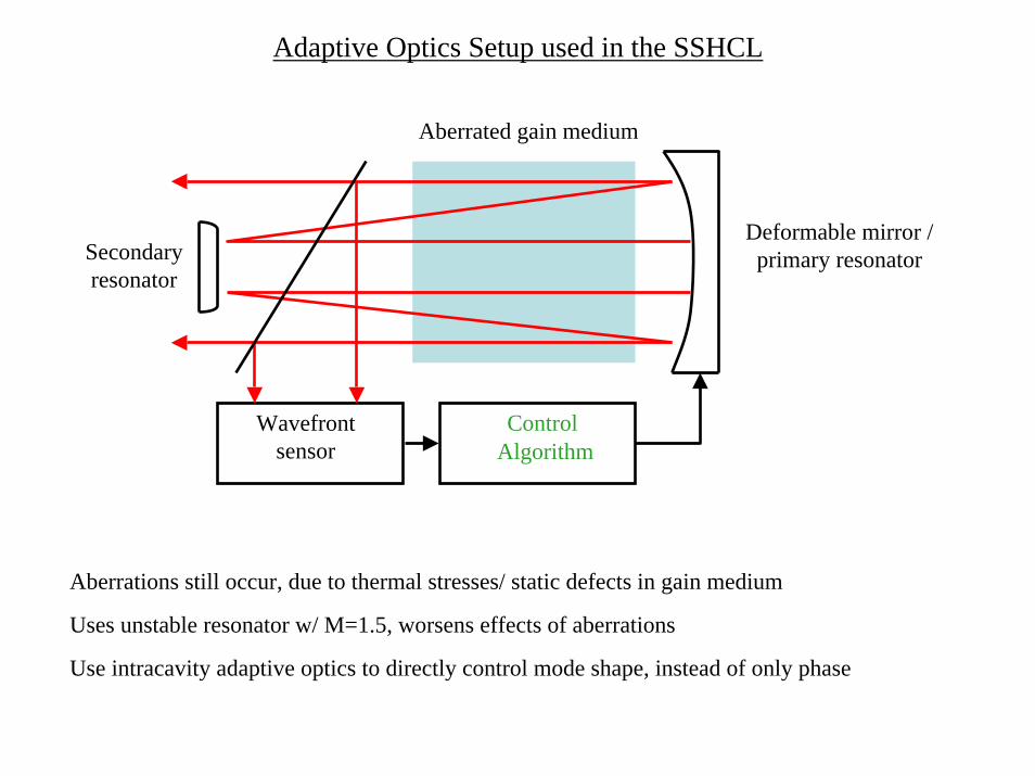
Adaptive Optics Setup used in the SSHCL

Aberrated gain medium

Deformable mirror / primary resonatorSecondary

resonator

Wavefront sensor

ControlAlgorithm

Aberrations still occur, due to thermal stresses/ static defects in gain medium

Uses unstable resonator w/ M=1.5, worsens effects of aberrations

Use intracavity adaptive optics to directly control mode shape, instead of only phase

Deriving AO Control Algorithm for SSHCL

Given an aberration measured by the WFS, what voltages should beapplied to the DM (deformable mirror) to correct it?

Resonator output phase for a given DM phase:

φout (x) = MW (zDM )M−1φDM (x)

• M - aberration polynomial mode construction operator

• W - mode influence coefficients, given the geometry of the resonator (diagonal matrix)

WFS measurement for a given DM voltage vector:

r s wfs = FMW (zDM )M−1D

r v DM ≡ A

r v DM

• F - finite difference operation representing WFS gradient operation

• D - influence of actuators of DM

• A - system matrix for that geometry

Use the least squares inverse to the system matrix:

r v DM = A+r

s wfs

Deriving AO Control Algorithm for SSHCL

• Ideal method for finding A: Measure convergent modal influence of each actuator using multipass resonation.

• Current: Assume A=FD (theoretically should converge). Measure A using a single pass through the system.

• Compromise: Detailed simulation to determine MWM-1 , or, numerical extrapolation of the system matrix gathered using the current method

Determining FD with a probe laser

Effect of resonation on Converged Actuator Influence Functions

• Impulse effect of actuator pushes are magnified, shifted, and summed-- shape and magnitude of converged wavefront are highly dependent of distance of actuator from optical axis

• Current testing cannot reveal converged influence function, because beam is not resonated.

• Can derive a more efficient control algorithm if know time averaged (converged) response

Off-axis influence function resonation

On-axis influence function resonation

Method for deriving effective modal influence of the actuators from the current, impulsive system matrix

1. Use current system matrix (actuator push vs. centroid slope data) to fit a DoG to 1d influence function of actuator in horizontal direction ( due to DM geometry, only sampling direction )

2. Exploiting 10% influence drop b/w adjacent actuators, extrapolate convergent 1d influence function to 2d influence function

3. Magnify the shift and width of the DoG according to the actuator’s location 30 times (effectively infinity), then sum together

D(x) = A0e−(b0x )2

− A1e−(b1x )2

1.0x10-6

0.8

0.6

0.4

0.2

Wav

elen

gths

(µm

)

100x10-3

806040200-20-40Displacement from actuator (mm)

2.5x10-6

2.0

1.5

1.0

Wav

elen

gths

(µm

)

-60x10-3

-40 -20 0 20 40 60Displacement from actuator (mm)

Multiple resonations of a 1d actuator influence function Resultant modal influence function

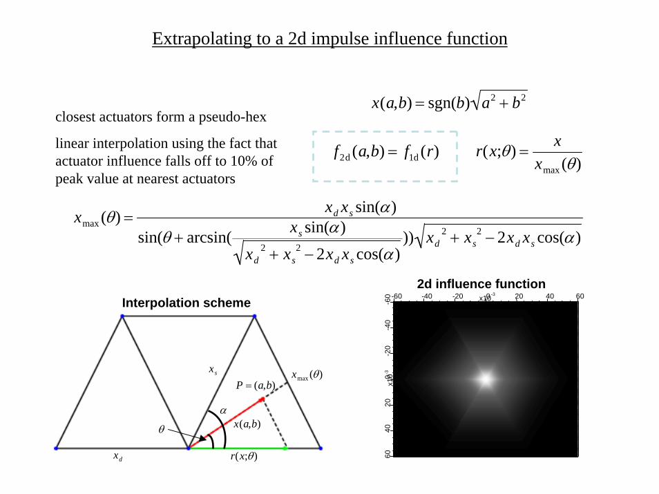
Extrapolating to a 2d impulse influence function

x(a,b) = sgn(b) a2 + b2

closest actuators form a pseudo-hex

linear interpolation using the fact that actuator influence falls off to 10% of peak value at nearest actuators

r(x;θ) =x

xmax (θ)f2d (a,b) = f1d (r)

xmax (θ) =xd xs sin(α)

sin(θ + arcsin( xs sin(α)xd

2 + xs2 − 2xd xs cos(α)

)) xd2 + xs

2 − 2xd xs cos(α)

2d influence function

6040

200

-20

-40

-60

x10-3

6040200-20-40-60 x10-3

Interpolation scheme

xmax (θ)xs

xd r(x;θ)

x(a,b)

P = (a,b)

α

θ

Evaluating accuracy of algorithm

• intensity variations (due to noise?), but same pattern

Input system matrix Predicted system matrix (1 resonation)

150

100

500

7006005004003002001000

150

100

500 7006005004003002001000

150

100

500 7006005004003002001000

150

100

500 7006005004003002001000

Comparisons and Conclusions

150

100

500 7006005004003002001000

• Much difference between the converged influence, and the impulse influence

• Since the converged influence accounts for effects of multiple passes through the resonator on the beam, it should lead to a more effective control algorithm

• Future directions: use more resonations, test the hypothesis that the converged influence provides a more efficient control algorithm, see effect of interpolative schemes on system matrices, …

Impulsive system matrix

150

100

500 7006005004003002001000

Converged system matrix

Acknowledgments

Kai LaFortune, Dr. Scot Olivier, and the Adaptive Optics Group at Lawrence Livermore National Laboratories

Lisa Hunter, Malika Moutawakkil, Hilary O’Bryan, the grad students, and the Center for Adaptive Optics

National Science Foundation (Grant #AST-987683)

References

Memo “Unstable resonator actuator modal influence functions”, by C. Brent Dane of LLNLTechnical Program Review: “Development of Adaptive Resonators for Solid State Heat

Capacity Lasers”. Brent Dane, Jim Brase, Erik Johansson, Scott Fochs, Mark Henesian, Jason Gwo.

Internal Document “The adaptive unstable resonator-- theory and design”. James M. Brase, Erik M. Johansson

EL FIN,

NADA MAS

Finding modal influence functions (1)

The modal influence function is a linear superposition of appropriately magnified impulse influence functions

Dmodal(x) = D(x) + M(D(x)) + M(M(D(x)) +L

Expand the width of the influence function without changing the amplitude and magnify the displacement of the influence function from the optical axis:

D(x) = A0e−(b0 (x−xc ))2

− A1e−(b1 (x−xc ))2 M⎯ → ⎯ DM (x) = A0e

−(b0

M(x−Mxc ))2

− A1e−(

b1

M(x−Mxc ))2

Impulse Influence function Modal influence function

1.0x10-6

0.8

0.6

0.4

0.2

0.0

-80x10-3

-60 -40 -20 0 20 40 60 80Displacement from actuator (mm)

A0 = 3.89247e-07A1 = -7.26713e-07b0 = -36.0892b1 = -150.226C = 6.54987e-09

Sampling/Fitting the 1D influence function

150x10-6

100

50

0

-50

-100

-150

Slo

pe

-80x10-3

-60 -40 -20 0 20 40 60 80Displacement from actuator (mm)

Centroid slopes vs. displacement

Height vs. displacement

Due to pseduo-hex geometry, can only sample meaningfully in the x-direction

Smoothness of fit to a DoG varies as increase sampling window width

Finding modal influence functions (2)

6040

200

-20

-40

-60

x10-3

6040200-20-40-60 x10-3

0.10

0.05

0.00

-0.0

5-0

.10-0.10 -0.05 0.00 0.05 0.10

Calculate a centered impulse with the necessary width for this resonation

Shift the impulse with the appropriate offset ( Mx, My)

6040

200

-20

-40

-60

x10-3

6040200-20-40-60 x10-3

Keep a running sum of the shifted impulses